


1. Introduction
Snow and avalanche climate classifications were initially developed to characterize the climate of mountainous regions, often to understand the conditions driving avalanche hazard (Roch, Reference Roch1949; LaChapelle, Reference LaChapelle1965; Armstrong and Armstrong, Reference Armstrong and Armstrong1987; McClung and Schaerer, Reference McClung and Schaerer2006). In hydrology, ecology and climate modeling, the term ‘snow climate’ has been employed to delineate seasonal average snow cover properties, including total depth, presence of depth hoar (DH), ice layers and snow temperature (Sturm and others, Reference Sturm, Holmgren and Liston1995). Within the field of snow avalanche studies, the term ‘snow climate’ specifically denotes the properties of the snow cover that are relevant for the formation of snow avalanches, thus proposing the term ‘snow and avalanche climate’ (Hägeli and McClung, Reference Hägeli and McClung2003). Understanding the snow and avalanche climate classification of a given mountain region is essential for developing location-specific avalanche mitigation and forecasting programs (e.g. McClung and Schaerer, Reference McClung and Schaerer2006).
The snow and avalanche climate classification has three primary patterns: Maritime, Continental and Transitional (LaChapelle, Reference LaChapelle1965). The Maritime climate is characterized by warm temperatures and heavy snowfall, with major instabilities predominantly attributed to recent snow loading and nonpersistent weak layers in the upper snow cover (Mock and Birkeland, Reference Mock and Birkeland2000; Haegeli and McClung, Reference Haegeli and McClung2007). Avalanche forecasting programs in these regions heavily rely on weather observations (McClung and Schaerer, Reference McClung and Schaerer2006). Conversely, the Continental snow and avalanche climate is distinguished by cold temperatures and low snowfall, high temperature gradient in the snow cover, creating persistent weak layers that necessitate systematic monitoring for forecasting snow avalanches (McClung and Schaerer, Reference McClung and Schaerer2006). The Transitional snow and avalanche climate exhibits characteristics of both Maritime and Continental snow and avalanche climates (Haegeli and McClung, Reference Haegeli and McClung2007). However, the description of a transitional snow and avalanche climate is often generalized and has been primarily delineated in western North America, and Haegeli and McClung Reference Haegeli and McClung(2007) suggesting that other regions experiencing varying degrees of continental and maritime influences should be included to enrich the understanding of this transitional snow and avalanche climate.
Mock and Birkeland Reference Mock and Birkeland(2000) introduced a flowchart aimed at classifying snow and avalanche climates, outlining snow cover processes pertinent to avalanche hazard assessment. Their approach utilized meteorological data to categorize individual winter seasons into distinct snow and avalanche climates. However, using only meteorological data is insufficient to describe snow instability, as Schweizer and others Reference Schweizer, Jamieson and Schneebeli(2003) demonstrated that the physical properties of slabs and weak layers serve as critical indicators of avalanche formation (Hägeli and McClung, Reference Hägeli and McClung2003). Recognizing this, Haegeli and McClung Reference Haegeli and McClung(2007) emphasized the necessity of incorporating additional snow stratigraphy information to refine the description of snow and avalanche climates. They proposed expanding the Mock and Birkeland Reference Mock and Birkeland(2000) flowchart to integrate avalanche and snow observations, particularly focusing on persistent weak layer observations, thus introducing the term ‘snow and avalanche climate’ (Haegeli and McClung, Reference Haegeli and McClung2007). This inclusion provides valuable insights into the percentage of avalanche activity on persistent weak layers and the specific types of persistent weak layers characterizing each snow and avalanche climate zone. This refinement is especially pertinent in delineating Transitional snow and avalanche climates, where the interplay of Continental and Maritime influences leads to distinctive persistent weaknesses in particular regions.
The concept of ‘avalanche problem type’ refers to a specific scenario of weather events and snow cover properties characterizing a type of snow instability that could lead to an avalanche. For example, a wind-deposited slab on a leeward slope or a persistent buried weak layer such as surface hoar (SH) crystals (called persistent slab) that could potentially lead to an avalanche (Statham and others, Reference Statham2018; EAWS, 2019). These avalanche problem types represent the primary concern for avalanche forecasters regarding specific meteorological and snow cover conditions, for example, a storm slab avalanche problem or wet avalanche problems. They are the foundation for various avalanche operational hazard forecasting to communicate the avalanche hazards in North America (Statham and others, Reference Statham2018) and Europe (Techel and others, Reference Techel, Karsten and Schweizer2020).
Building upon this framework, Shandro and Haegeli Reference Shandro and Haegeli(2018) integrated avalanche problem data type with the Mock and Birkeland Reference Mock and Birkeland(2000) flowchart to enhance the characterization of snow avalanche hazard in western Canada. While the methodology of Mock and Birkeland Reference Mock and Birkeland(2000) offers a generalized description of snow and avalanche climate across multiple winter seasons, the incorporation of avalanche problem type data facilitates a more nuanced understanding, addressing daily concerns for forecasters throughout the season. However, building a temporally extensive database of snow observations and forecasted avalanche problem types can be difficult without avalanche forecasting data. To fill this gap and to provide an independent methodology, Reuter and others Reference Reuter(2022) proposed a method to derive avalanche problem types from snow cover model output such as SNOWPACK (Lehning and others, Reference Lehning, Bartelt, Brown, Russi, Stockli and Zimmerli1999) or SURFEX/CROCUS (Vionnet and others, Reference Vionnet2012). This method allows us to characterize avalanche problems, based on snow cover modeling, for instance, and hence, omitting the use of avalanche forecasting data.
Various combinations of the methodologies outlined above have been employed to describe and classify additional regions, utilizing different data types primarily based on data availability. For instance, Ikeda and others Reference Ikeda, Wakabayashi, Izumi and Kawashima(2009) utilized the Mock and Birkeland Reference Mock and Birkeland(2000) flowchart alongside snow cover data to delineate the snow and avalanche climate of the Japanese Alps. Their findings for the Japanese Coastal mountains exhibited similarities with the Maritime climate zone. However, the Central Japanese Alps, characterized by a thin snow cover, cold temperatures conducive to persistent weak layers development, and a significant amount of rainfall, did not align with any of the three main snow and avalanche climates. Consequently, they introduced the term ‘Rainy Continental’ for the Central Japanese Alps (Ikeda and others, Reference Ikeda, Wakabayashi, Izumi and Kawashima2009). Similarly, Eckerstorfer and Christiansen Reference Eckerstorfer and Christiansen(2011) utilized snow profile data to describe the snow and avalanche climate of Svalbard’s main settlement, Longyearbyen. Their analysis highlighted a thin snow cover, persistent weaknesses and substantial ice layers attributed to maritime influences, which led them to propose the term ‘High Arctic Maritime’ for Central Svalbard (Eckerstorfer and Christiansen, Reference Eckerstorfer and Christiansen2011). Recently, Reuter and others Reference Reuter, Hagenmuller and Eckert(2023) characterized the snow and avalanche climate of the French Alps, as well as Schweizer and others Reference Schweizer, Knappe, Reuter and Mayer2024 in the Swiss Alps. Both of these studies used two approaches, the snow and avalanche climate classification algorithm of Mock and Birkeland Reference Mock and Birkeland(2000) and the frequency of avalanche problem types based on snow cover simulations. With their approach, they put forward the idea of classifying snow and avalanche climates based on avalanche problem type occurrences. Their comparisons with the standard snow and avalanche climate classification suggest that adding the avalanche problem occurrences provides for a more detailed characterization.
In Eastern Canada, the Chic-Chocs mountains in the Gaspé Peninsula are prone to snow avalanches. Multiple studies have highlighted the influence of snowstorms and thaw events on the local snow avalanche dynamic (Germain and others, Reference Germain, Filion and Hétu2009; Hétu, Reference Hétu2010; Fortin and others, Reference Fortin, Hétu and Germain2011; Gauthier and others, Reference Gauthier, Germain and Hétu2017). Despite the classic climate classification of Köppen indicating a humid continental climate, the region experiences a significant maritime influence, complicating the classification of the snow and avalanche climate (Gagnon, Reference Gagnon1970; Fortin and others, Reference Fortin, Hétu and Germain2011; Gauthier and others, Reference Gauthier, Germain and Hétu2017). While the winter climate of the region has been extensively documented (Gagnon, Reference Gagnon1970; Fortin and others, Reference Fortin, Hétu and Germain2011; Fortin and Hétu, Reference Fortin and Hétu2014; Gauthier and others, Reference Gauthier, Germain and Hétu2017), the description primarily relies on seasonal average climate conditions not directly relevant to avalanche formation. Hence, comprehensive analysis integrating snow cover and weather data relevant to avalanche formation holds promise to elucidate the region’s snow and avalanche climate.
Given the presence of established approaches in snow climatology and the importance of better understanding the snow and avalanche climate of the Chic-Chocs mountains, our aim was to (1) describe the snow and avalanche climate for the Chic-Chocs mountains, (2) compare the dataset Chic-Chocs region with other mountain ranges such as Mount Washington (New Hampshire, USA), Central Japan and the French Alps. We conclude the paper by discussing how the current snow and avalanche climate observed in the Chic-Chocs could evolve regarding climate change.
1.1. Study area
This study focuses on the Chic-Chocs mountains, a northern extension of the Appalachian Mountains, which forms an inland massif serving as the backbone of the Gaspé peninsula (Fig. 1). This central massif comprises sub-alpine and alpine terrain, ranging in elevation from 800 to 1200 meters above sea level (m a.s.l.), and is encompassed by a lower plateau situated at 400–500 m a.s.l. (Fig. 1). The study area is mainly the Avalanche Québec forecasting area. This nonprofit organization has been issuing avalanche bulletins for backcountry users in the Chic-Chocs since 2000. Since Avalanche Québec is now part of the Avalanche Canada forecasting program, the organization could benefit from a snow and avalanche climate description to tailor their procedures from well-established procedures in western Canada.
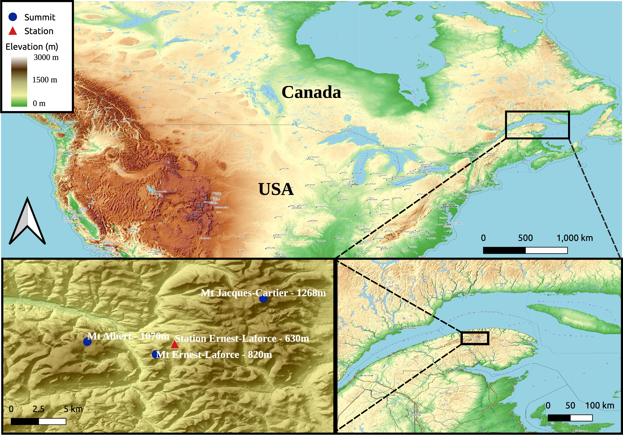
Figure 1. Localization map of the study inside North America. The input represents different spatial scale of the study area with the different summits around the weather station Ernest-Laforce 630 m. The background map is from opentopomap.org and the elevation model of Canada from Natural Resources Canada.
The Chic-Chocs region receives ∼800 mm of precipitation annually, while the high plateau of the interior receives around 1600 mm (Gagnon, Reference Gagnon1970; Germain and others, Reference Germain, Hétu and Fillion2010; Fortin and others, Reference Fortin, Hétu and Germain2011). Snowfall typically occurs from December to April, accompanied by an average of about 60 mm of rainfall per winter (Fortin and others, Reference Fortin, Hétu and Germain2011). The mean annual temperature, spanning from 1971 to 2010, varies from 3∘C along the Gaspé North Coast to  $-4^\circ$C at 1268 m (Mount Jacques-Cartier) (Gray and others, Reference Gray, Davesne, Fortier and Godin2017). The regional climate exhibits contrasting weather patterns: (1) cold Arctic air masses often bring northwesterly winds with temperatures dropping below $-20^\circ$C, and (2) continental low-pressure systems, usually accompanied by northeasterly winds, resulting in temperatures near the freezing point and potential rain. These weather systems, commonly referred to as the Alberta Clipper, the Colorado Low and the Hatteras Low, significantly influence the Gaspé Peninsula’s weather, impacting the type of precipitation experienced in the area (Fortin and Hétu, Reference Fortin and Hétu2014). The interaction of these weather patterns with the peninsula’s topographic features creates a snow accumulation pattern conducive to avalanche formation (Germain and others, Reference Germain, Hétu and Fillion2010). Most avalanches in the region are natural releases occurring during storms (Germain and others, Reference Germain, Filion and Hétu2009; Hétu, Reference Hétu2010; Fortin and others, Reference Fortin, Hétu and Germain2011; Gauthier and others, Reference Gauthier, Germain and Hétu2017).
2. Methods
2.1. Classification strategy
To provide a comprehensive description of the snow and avalanche climate, we used several methodologies drawn from work on snow and avalanche climatology widely used over the past decades (Sturm and others, Reference Sturm, Holmgren and Liston1995; Mock and Birkeland, Reference Mock and Birkeland2000; Shandro and Haegeli, Reference Shandro and Haegeli2018; Reuter and others, Reference Reuter2022). While these methodologies formed the basis of our approach, we adapted them by selectively incorporating relevant aspects tailored to our specific research needs. This approach integrated several types of data relevant to understanding avalanche formation.
We used the Mock and Birkeland Reference Mock and Birkeland(2000) flowchart, which uses observed and simulated climate data to outline the general snow and avalanche climate. We then retrieved from snow cover simulations the distribution of snow grain types for the whole snow cover described by Sturm and others Reference Sturm, Holmgren and Liston(1995), and also for the critical weak layers. These snow cover data not only clarify the dominant metamorphic processes but also help to identify which snow grain types characterized the weak layers of the study area. In addition, we have included avalanche problem types to characterize avalanche hazard, inspired by the approach of Shandro and Haegeli Reference Shandro and Haegeli(2018). The avalanche problem types were derived from simulations with the SNOWPACK model (Lehning and others, Reference Lehning, Bartelt, Brown, Russi, Stockli and Zimmerli1999), following the framework described in Reuter and others Reference Reuter(2022). They characterize snow instability patterns for every day. This type of data complements the description of the snow and avalanche climate.
Finally, similarly to Reuter and others Reference Reuter, Hagenmuller and Eckert(2023), a temporal cluster analysis of the avalanche problem type has been performed over the 40 year period from 1982 to 2022. This analysis should show the different types of winters that the region can experience, while providing a different point of view from the classic snow and avalanche climate classification of Mock and Birkeland Reference Mock and Birkeland(2000), developed in western North America. Because we used the same methodology of Reuter and others Reference Reuter(2022), a direct comparison of the results can be done with the French Alps and describe the snow and avalanche climate in reference to the frequency of avalanche problem types (Shandro and Haegeli, Reference Shandro and Haegeli2018; Reuter and others, Reference Reuter, Hagenmuller and Eckert2023). It is important to note that the database includes data representing the winter avalanche regime from December 1 through March 31. Data representing the spring avalanche regime were not included in this analysis.
2.2. Meteorological data
Meteorological data were collected at a weather station located in the Chic-Chocs range. The weather station, named Ernest-Laforce weather station (CAELA), is located on the north slope of Mount Ernest-Laforce at 630 m a.s.l. (Fig. 4). The dataset covers the winter seasons from December 1 to March 31 for the winter seasons 2012–13 to 2021–22. Hourly data for mean air temperature, snow height (HS) (ultrasonic HS sensor) and precipitation (measured using a weighing precipitation gauge) were used to calculate the meteorological variables required for the Mock and Birkeland Reference Mock and Birkeland(2000) flowchart: daily mean air temperature (meanTA, ∘C), total snowfall (cm), total snow precipitation water equivalent (SWE in mm), total rain (mm) and mean December snow cover temperature gradient (meanDECTG, ∘C m−1). Rain and SWE were derived from total precipitation using a rain/snow threshold of 1.2∘C with the mean hourly air temperature. This threshold is the default SNOWPACK snow/rain threshold, which was empirically determined based on measurements in Switzerland (Lehning and others, Reference Lehning, Bartelt, Brown, Russi, Stockli and Zimmerli1999). To minimize misclassification of precipitation events, snow events were confirmed by a significant increase (>2 cm) in HS within the next 2 hours after the precipitation event. Rain events were similarly validated by stable or decreasing HS during the rain event. The underestimation of the snow precipitation gauge is well known, but the CAELA weather site is a forested site with low wind speed, which should minimize the undercatch effect of the precipitation gauge (Fassnacht, Reference Fassnacht2004). The total snowfall was derived using the sum of the difference between the present hourly HS and the prior hourly HS. Using the hourly difference in HS, we reduce the influence of the new snow settlement. The mean temperature gradient in December was determined using the mean air temperature and the mean HS for December, assuming 0∘C at the snow–soil interface (Mock and Birkeland, Reference Mock and Birkeland2000). The observed meteorological indicators used in the Mock and Birkeland Reference Mock and Birkeland(2000) algorithm are used as a basis to compare the same meteorological indicators derived from the climate simulation presented below.
2.3. Climate simulation data
To increase the temporal extent of this study and to complement the use of only one altitude weather station, climate model simulations were used. Climate models represent different components of the climate system, such as the atmosphere, ocean, land surface, ice and ecosystems, and are integrated to project the climate of a particular region or domain. In this research, we use the sixth generation of the Canadian regional climate model (CRCM6/GEM5.0), which is currently under development at the Centre pour l’Étude et le Simulation du Climat à l’Échelle Régional (ESCER) of the University of Quebec at Montréal (UQAM). Two studies have recently used this newly improved model from the established GEM4.0 in North America (Moreno-Ibanez and others, Reference Moreno-Ibanez, Laprise and Gachon2023; Roberge and others, Reference Roberge, Luca, Laprise, Lucas-Picher and Thériault2024). The version of CRCM6/GEM5.0 used in this study is based on version 5.0.2 of the Global Environmental Multiscale Model (GEM5) (Girard and others, Reference Girard2014; McTaggart-Cowan and others, Reference McTaggart-Cowan2019), which serves as the operational numerical weather prediction model for the Meteorological Service of Canada. The CRCM6 model uses a 12 km (0.11∘) spatial grid based on the Regional Deterministic Prediction System (RDPS) configuration of the 5.0.2 version of the Global Environmental Multiscale Model (GEM5) (Girard and others, Reference Girard2014; McTaggart-Cowan and others, Reference McTaggart-Cowan2019). This model was chosen for its spatial downscaling capabilities and hourly time step, which we selected from 1982 to 2022.
To increase the overall representativeness of the modeled data, four grid points were selected around the coordinates of the CAELA weather station, and the mean value was extracted. The data were provided and processed by the ESCER. The mean elevation of the four grid points is 679 m, which represents a slight overestimation of the actual weather station, which is at 630 m. Based on methodologies from Bellaire and others Reference Bellaire, Jamieson and Fierz(2011), Coté and others (Reference Coté, Madore and Langlois2017) and Imbach and others (Reference Imbach, Gauthier and Langlois2024) observed an underestimation of total precipitation and snowfall quantities for the CRCM6 model at the CAELA weather station study site. The underestimation was rate dependent, meaning that the underestimation of the precipitation quantities increases with the intensity of the precipitation. In order to correct this underestimation, both the hourly precipitation were categorized into linear equal precipitation intensity classes (2 mm h−1 increment from 0 to 12 mm h−1). The median of each precipitation class was then used to correct both the hourly precipitation data (both rain and snow). This process was applied to the entire hourly dataset from 1981 to 2022. The resulting simulated HS from this correction will be compared to the non-corrected simulated precipitation (CRCM6) and the in situ HS at CAELA.
2.4. Meteorological data from other locations
To compare our data with potentially similar locations around the globe and existing snow and avalanche climate classification, we adapted the boxplot figure from Mock and Birkeland Reference Mock and Birkeland(2000), incorporating each of the climate indicators to visually compare the mentioned regions. We also used data directly from the snow study of Ikeda and others Reference Ikeda, Wakabayashi, Izumi and Kawashima(2009) for the Central Japanese Alps and data from Mount Washington in New Hampshire, USA (Meloche, Reference Meloche2019), which is also similar to the Chic-Chocs.
2.5. Snow cover modeling
The snow cover model SNOWPACK is a multilayer one-dimensional thermodynamic model and was used to simulate the snow cover stratigraphy and properties for each snow season (Lehning and others, Reference Lehning, Bartelt, Brown, Russi, Stockli and Zimmerli1999). The required meteorological data inputs were driven from the CRCM6 model, which were air temperature, relative humidity, wind speed and direction, short and longwave radiation (incoming and outgoing), total precipitation and HS. In this study, SNOWPACK was run using hourly CRMC6 data with HS forcing. The model parameters were based on previous work and validation performed by members of the research team for the same study area (Coté and others, Reference Coté, Madore and Langlois2017) and also in western Canada (Madore and others, Reference Madore, Langlois and Coté2018, Reference Madore, Fierz and Langlois2022). We chose to use the default SNOWPACK snow/rain threshold of 1.2∘C, and the main parameterizations (SNOWPACK parameters) used were the BELLAIRE snow density parameterization, the MONTI hardness parameterization, the Bucket water percolation model and the MO-MICHLMAYR atmospheric stability. The SNOWPACK simulation was forced with the HS predicted by the CRCM6 model for the 40 year period from 1982 to 2022. We present a comparison with two simulated HSs, one from the HS forcing and one from the precipitation forcing. We computed performance metrics such as the mean relative error (MRE) and the root-mean-square error (RMSE). The snow cover was simulated every hour from October 1 to May 31 to ensure a proper simulation of the entire snowpack, on the flat and also on two 38∘ virtual slopes on a northern and southern aspect. Wind transport and wind erosion parameters in SNOWPACK were activated on the virtual slopes simulations, meaning that additional snow accumulation or HS reduction is possible due to wind on the virtual slopes.
2.6. Snow grain type
The seasonal snow grain type distribution was computed from the snow cover model output by adding the thickness of each layer to a snow grain type class such as precipitation particles (PP), melt forms (MF) or faceted crystals (FC). This process is repeated daily from December 1 to March 31 to analyze only the ‘winter’ grain type and avoid overrepresentation of wet grain during spring. These dates were also chosen for consistency with the methodology of Mock and Birkeland Reference Mock and Birkeland(2000). The frequency distribution is normalized by the sum of all layer thicknesses for both north and south virtual slopes during the winter from December to March.
In order to assess the validity of the snow grain type obtained from the snow cover model, we compared it with the seasonal snow grain type frequency retrieved from snow profile observations throughout the season. These observations were made by Avalanche Québec, which is responsible for avalanche forecasting in the Chic-Chocs region, for the winter of 2015–18 (Meloche, Reference Meloche2019). The snow profiles were made at different aspects and elevations throughout the region, with ∼25 snow profiles per winter.
2.7. Avalanche problem type
2.7.1. Weak layer identification
The avalanche problem type was derived from the output of the SNOWPACK model, i.e. from both north- and south-facing slope simulations, following the methodology proposed by Reuter and others Reference Reuter(2022). The following section describes the general procedure of the method, for more details please refer to the original paper. This method evaluates potential persistent and nonpersistent instabilities on each day, which could be either prone to natural release or artificial triggering. For the purpose of this study, only natural release was considered. The nonpersistent weak layer is composed of either PP, decomposed and fragmented particles (DF) or faceted rounded grains (FCxr). The persistent weak layers are composed of faceted crystals (FC - FCxr), SH crystals and DH crystals.
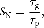
If a potential weak layer was present the day before or potentially buried, the properties of the slab overlaying this potential weak layer are judged. A minimum slab thickness of 0.18 m and a slab density of at least 100 kg m−3 are required for a critical slab-weak layer combination (Reuter and others, Reference Reuter2022). Four indices were then used to classify all potential slab-weak layer combinations in view of natural release. The  $S_\mathrm{N}$ (natural) index was computed for each layer within the snowpack, defined by a ratio of the gravitational shear stress $\tau_\mathrm{g}$ induced by the weight of the overlying slab and the shear strength of the weak layer:
 \begin{equation}
S_\mathrm{N} = \frac{\tau_\mathrm{g}}{\tau_\mathrm{p}},
\end{equation}
\begin{equation}
S_\mathrm{N} = \frac{\tau_\mathrm{g}}{\tau_\mathrm{p}},
\end{equation} where 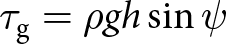 $\tau_\mathrm{g} = \rho g h \sin{\psi}$ is defined by the slab density ρ, the gravitational acceleration g, the slab height h and the slope angle ψ. The time to failure
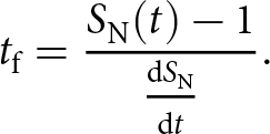
  $t_\mathrm{f}$ was also used to determine the natural stability of the layers, developed by Conway and Wilbour Reference Conway and Wilbour(1999). The time to failure is the time derivative of $S_\mathrm{N}$:
 \begin{equation}
t_\mathrm{f} = \frac{S_\mathrm{N} (t) -1}{\frac{\mathrm{d}S_\mathrm{N}}{\mathrm{d}t}}.
\end{equation}
\begin{equation}
t_\mathrm{f} = \frac{S_\mathrm{N} (t) -1}{\frac{\mathrm{d}S_\mathrm{N}}{\mathrm{d}t}}.
\end{equation} A second stability indicator is the critical crack propagation length  $a_\mathrm{c}$, which is the length required for crack propagation to begin. It can be derived from the SNOWPACK simulation based on stress and strength approach (Gaume and others, Reference Gaume, Van Herwijnen, Chambon, Wever and Schweizer2017) or using the weak layer fracture energy (Heierli and others, Reference Heierli, Gumbsch and Zaiser2008). We derived the weak layer fracture energy and solved for the critical crack length (Schweizer and others, Reference Schweizer, van Herwijnen and Reuter2011) through finite element calibrations (van Herwijnen and others, Reference van Herwijnen, Gaume, Bair, Reuter, Birkeland and Schweizer2016). The weak layer fracture is estimated from the squared simulated shear strength (Gaume and others, Reference Gaume2014). To avoid using finite element simulations, we compute an average slab modulus from the density and thickness of the slab (Scapozza and others, Reference Scapozza, Bucher, Amann, Ammann and Bartelt2004).
Based on these three indices, we classified each potential layer as an unstable weak layer using the thresholds determined by Reuter and others Reference Reuter(2022). A weak layer was classified as critical for natural release if  $S_\mathrm{N} \lt 3.6$ and $t_\mathrm{f} \lt 18$ hours, and $a_\mathrm{c} \lt 0.32$ m. Then, for each unstable weak layer, we classified it as a persistent or nonpersistent weak layer depending on the weak layer grain type. The snow grain types of each critical weak layer were counted to get a frequency of weak layer snow grain type over the simulated 40 year period.
2.7.2. Assigning avalanche problem
The following avalanche problem types were derived from the SNOWPACK model output: new snow (AP_newsnow), wind slab (AP_wind), persistent (AP_persistent) and wet (AP_wet), based on the methodology developed by Reuter and others Reference Reuter(2022). On each day, after classifying the critical persistent and nonpersistent weak layers, we look at the concurrent snow load modeled in SNOWPACK. A nonpersistent weak layer within a 24 hour snowfall (HN24) >5 cm is classified as a new snow problem (AP_newsnow). If a persistent critical weak layer is loaded by a precipitation rate >0.05 m/24 h, the algorithm will classify it as a persistent avalanche problem (AP_persistent) and a new snow avalanche problem (AP_newsnow). The same procedure is used for a wind slab avalanche problem (AP_wind) with a 24 hour wind transport (wind_trans24) >0.4 m/24 h and a nonpersistent weak layer. A AP_wind is also possible if the wind_trans24 is above the threshold and soft snow is present on the surface within 3 days. The algorithm will classify both a AP_persistent and AP_wind when the wind transport threshold is reached with an unstable persistent weak layer.
The assessment of the wet-snow avalanche problem is based on the liquid water content index developed by Mitterer and Schweizer Reference Mitterer and Schweizer(2013) along with the number of days since isothermal conditions were reached (Baggi and Schweizer, Reference Baggi and Schweizer2009). This index measures the liquid water per snow volume for each SNOWPACK layer, with an averaging process that considers the thickness of these layers to determine the total liquid water content of the snow cover. The index compares the total water content of the snow cover to a critical threshold of 3% water per ice volume (Mitterer and others, Reference Mitterer, Heilig, Schmid, Van Herwijnen, Eisen and Schweizer2016). A liquid water content index of 1 indicates the onset of natural wet-snow avalanches, then, the snow cover returns to a stable state after 4 days of sustained isothermal conditions (Baggi and Schweizer, Reference Baggi and Schweizer2009). We assign the avalanche problem for both the virtual north and south face slope of every winter of the 40 year period. We used the find_aps.py function, in the package the snowpacktools from the public repository of the Avalanche Warning Service Operational Meteo Environment (AWSOME Core Team, 2024).
In order to assess the validity of the avalanche problem type derived from the SNOWPACK modeling, we compared it with the forecasted avalanche problem type from Avalanche Québec for the winter of 2012–18 (Meloche, Reference Meloche2019). The predicted avalanche problem types are the forecaster’s assessment for the upcoming forecast period based on meteorological observations, snow cover observations and weather forecasts. The forecast period was 2 days for winters 2013–15 and daily for winters 2016–18.
2.8. Clustering
Finally, we performed a k-means cluster analysis to explore a different classification of the avalanche characteristics of the study area. The k-means is a clustering analysis that uses the proximity to a geometric position in the feature coordinate space (Macqueen, Reference Macqueen1967). The k-means was applied to the north- and south-facing slope simulations for the avalanche problem type, covering the 40 year period from 1982 to 2022. We neglected the climate indicators and the snow grain type to reduce dimensionality and to replicate the same method as Reuter and others Reference Reuter, Hagenmuller and Eckert(2023). In addition, the avalanche problem type integrates the weather context and snow grain type from the critical weak layer. To select the ideal number of clusters, we computed the Silhouette score and the Calinski–Harabasz score for a number of clusters ranging from 2 to 10. Silhouette score values help determine the optimal number of clusters and assess clustering quality. They measure how well a data point fits within its assigned cluster compared to neighboring clusters. Values close to 1 indicate a proximity within its cluster, values near 0 suggest ambiguity and negative values signal potential misclassification. In addition, the Calinski–Harabasz score evaluates the balance between the variance within clusters and the variance between clusters, by minimizing the ratio of within-cluster variance to between-cluster variance, ensuring well-separated and compact clusters (Harabasz and Karoński, Reference Harabasz and Karoński1974).
We selected the number of clusters with the maximum values of Silhouette score per number of clusters and Calinski–Harabasz score. The number of clusters when one of the individual clusters was below the average Silhouette score was not considered. We also performed a principal component analysis (PCA) on the avalanche problem type dataset to explore linearity between variables and to facilitate visualization of our clustering results. In addition, the result of the clustering analysis will be compared to the French Alps where a similar analysis was made by Reuter and others Reference Reuter, Hagenmuller and Eckert(2023). The frequency of avalanche problem types of the French will provide a basis for comparison of the frequency observed in the Chic-Chocs.
3. Results
3.1. Snow and avalanche climate classification
3.1.1. 10 years of meteorological data
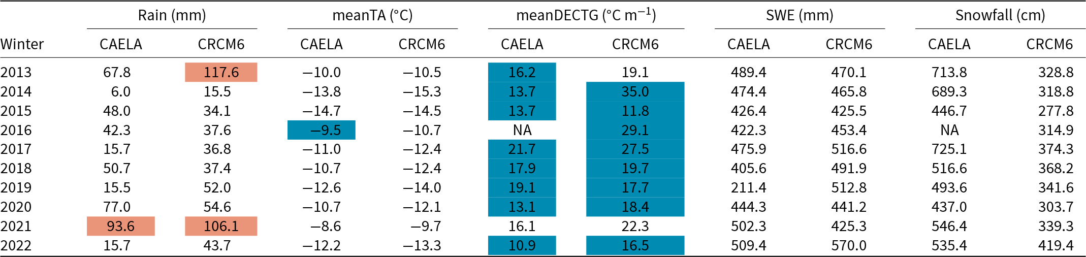
As a first result, we present 10 years (2013–22) of meteorological data recorded at the Mount Ernest-Laforce weather station and data simulated by the climate model CRCM6. The Chic-Chocs study area generally exhibited cold average winter temperatures (meanTA  $ \lt -7^\circ$C) and limited total winter snow precipitation (Snow < 450 mm SWE). The winters of 2016 and 2021 showed warmer conditions, but only the winter of 2021 showed significant rain during the winter season (Table 1). The winters of 2013 and 2020 were also warmer, with a significant amount of rain (67.8 and 77.0 mm, respectively). For all winters, the meanTA fell below $-7^\circ$C, and the meanDECTG was consistently above 10∘C m−1. This combination of cold mean air temperatures and sparse snow cover likely contributed to the pronounced temperature gradients observed (Table 1).
Table 1. Results of the Mock and Birkeland Reference Mock and Birkeland(2000) classification with weather station Mount Ernest-Laforce and the CRCM6 climate model. The year in the column winter represents the month of January, indicating that the winter of the present year includes December of the prior year. The light blue indicates a continental classification with this climate indicator and the light red a maritime classification. Mean winter air temperature is denoted meanTA, the mean December temperature gradient (meanDECTG) and the snow precipitation water equivalent (SWE)
The average HS at CAELA weather station is 116 cm from 2012 to 2022 and the maximum HS reached 248 cm. Figure 2a shows the HS evolution of the winter 2018, and the average over 10 years from 2012 to 2022 with the standard deviation (Fig. 2b). The simulated HS from different parameterizations of the model chain CRCM6/SNOWPACK. The two dashed lines representing the simulated HS without the precipitation rate correction are the two lowest HS for 2018 (Fig. 2a) and also for the mean over 10 years (Fig. 2b). The SNOWPACK simulation forced on the precipitation (Psum) was the lowest HS between the parameterizations. The two forced parameterizations with the HS and the precipitation rate correction were the closest to the in situ HS. Figure 2 demonstrates the added values of the correction and the simulation enforced by HS at CAELA with MRE of 36% and an RMSE of 35.7 cm, compared to the simulation enforced by Psum with the correction (MRE = 189% and RMSE = 51 cm).
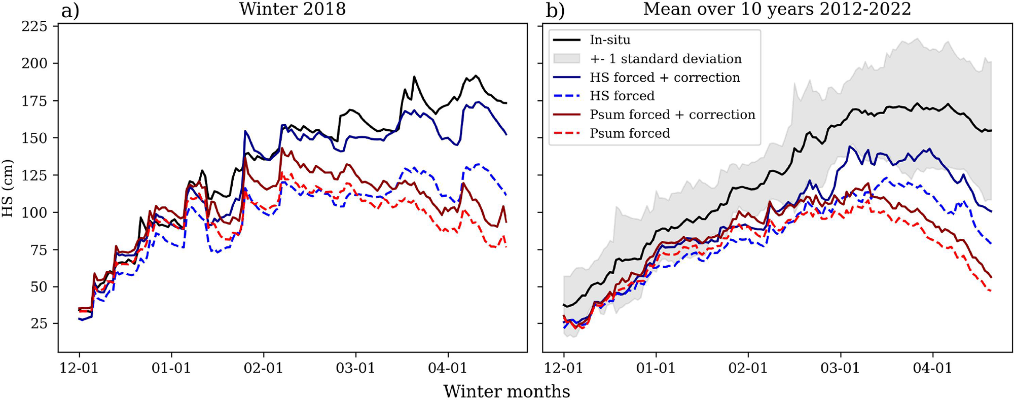
Figure 2. Snow height (HS) temporal evolution, including the in situ measurement at CAELA, the simulated HS (SNOWPACK), enforced either by the HS or precipitation (Psum), with or without the precipitation rate correction, over the (a) winter 2018, (b) mean over 10 years (2012–22). The light gray background corresponds to 1 standard deviation from the mean HS in situ at CAELA weather station.
Figure 3 shows the difference between the CAELA weather station and the CRCM6 model. The snow precipitation (SWE) estimation with the CRCM6 model is relatively good with an MRE of 17%. Because of the precipitation correction, there is no systematic underestimation of precipitation (SWE), which has no clear systematic bias with SWE being underestimated and others overestimated (Fig. 3). However, despite the precipitation correction and the HS forcing in SNOWPACK, the HS and snowfall were underestimated by the CRCM6 model with respectively a negative MRE of −15% and −38%. Rain has the most significant error, with an MRE of 77%, and no clear bias (Fig. 3). The CRCM6 model simulated colder temperatures compared to the weather observations (MRE 9%) (Fig. 3). Finally, CRCM6 slightly overestimated the mean temperature gradient in December (MRE 23%), with less simulated HS.
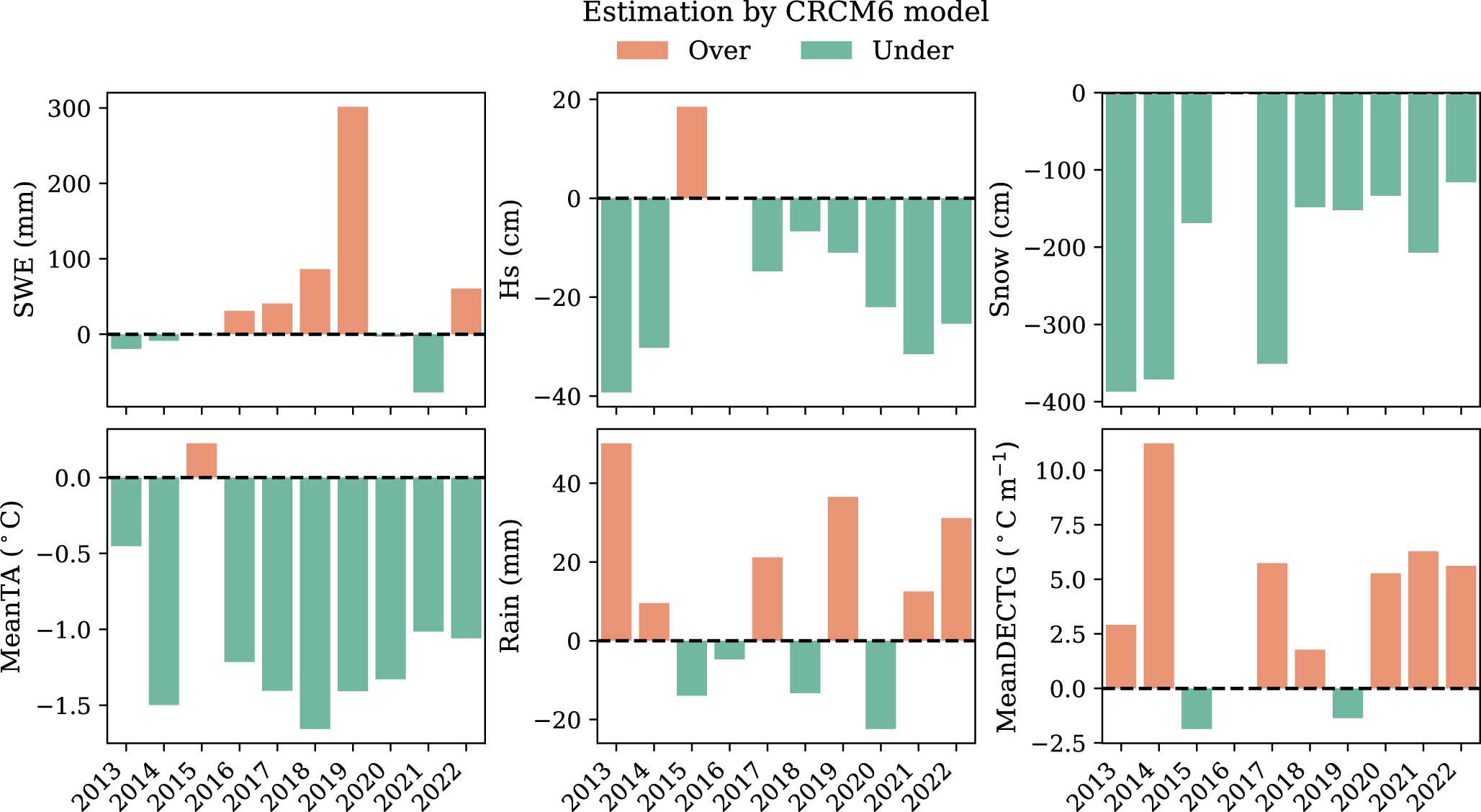
Figure 3. Estimation of the climatic indicators used in Mock and Birkeland Reference Mock and Birkeland(2000) algorithm by the CRCM6 model, with snow height (HS) in addition. The estimation is compared to the weather observations at the CAELA station. The positive difference represents an overestimation (orange) of the CRCM6 model, and the negative difference represents an underestimation (green) of the CRCM6 model.
The results of the snow and avalanche climate classification derived from the Mock and Birkeland Reference Mock and Birkeland(2000) flowchart indicated a predominantly continental climate for in eight out of ten winters and a maritime classification for the remaining two winters (Table 1). The winter 2013 had a continental classification at the weather station but a maritime classification with the CRCM6 model. The key determinant in classifying most continental winter seasons was the mean December temperature gradient (meanDECTG), which exceeded 10∘C m−1 for a continental climate and rain amounts exceeding 80 mm for a maritime climate (Table 1). The algorithm never met the ‘snow accumulation’ criterion for classification into maritime and transitional snow and avalanche climates during the classification process for both weather data (weather station and CRCM6) (Table 1).
3.1.2. 40 years snow and avalanche climate classification
Figure 4 shows a time series of the rain and mean air temperature for the last 40 winters (1982–2022) simulations from the CRCM6 model. The classification results are also shown by the background color for each year where blue is for continental and red for maritime, as the transitional snow and avalanche climate was never classified for the 40 winters. The rain indicator was the only indicator that classified some winters as maritime (above the dashed line in Fig. 4). Most of the winters (33/40) were classified as continental based on the mean December temperature (meanDECTG). The mean air temperature is relatively cold and never exceeds  $-8^\circ$C, which is far from the $-3^\circ$C threshold for a maritime winter. Some winters have been classified as maritime (7/40), and these winters are spread over the entire 40 year period. Despite the generally cold temperatures, rain events occur almost systematically every winter. Rain-on-snow events during the winter combined with cold air temperature (meanTA $ \lt -7^\circ$C) are the two main characteristics that define the region’s snow and avalanche climate.
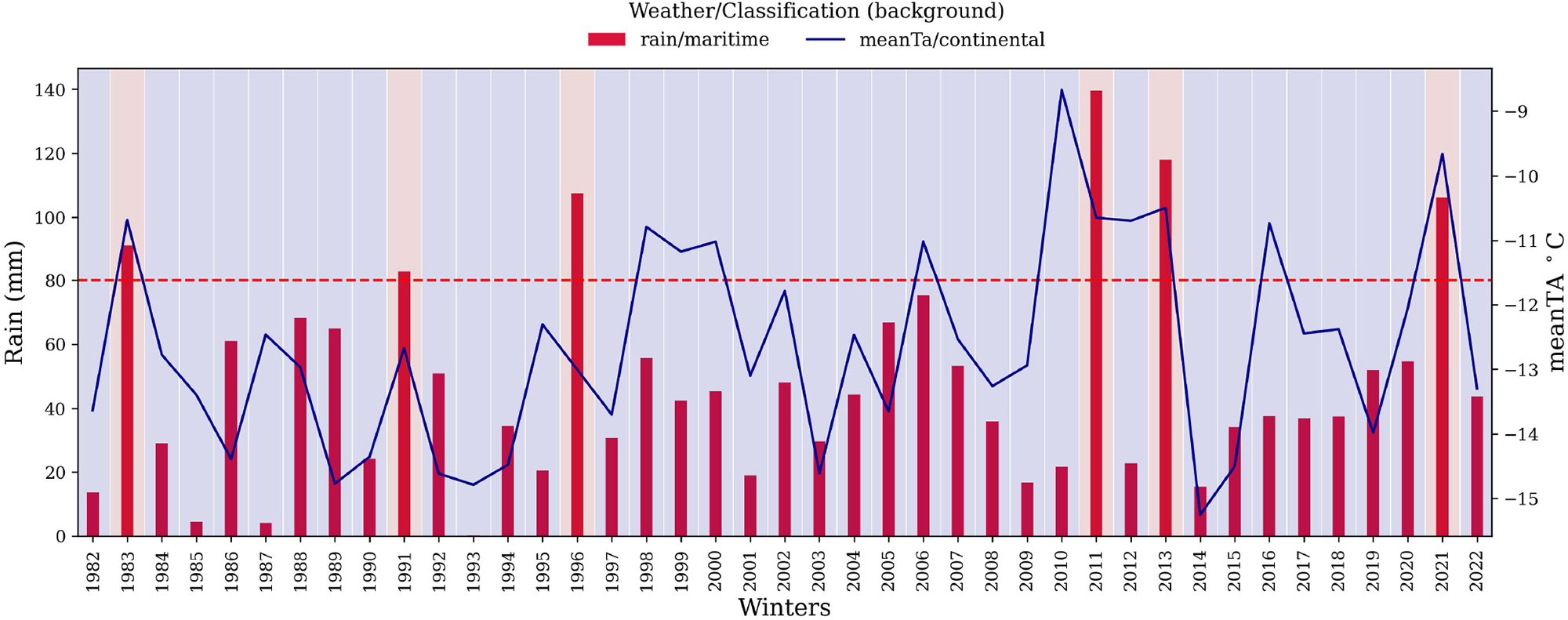
Figure 4. Time series of the mean air temperature and total rain for the winters 1982 to 2022. The result of the Mock and Birkeland Reference Mock and Birkeland(2000) classification is shown with background color for each winter: the blue color is a continental classification, red is for maritime, transitional was never present. The mean air temperature is shown in dark blue and the total rain during the winter is shown in dark red. The black dashed line represents the 80 mm rain threshold for the maritime classification.
3.1.3. International comparison
To compare our data with potentially similar locations around the globe, we adapted the boxplot figure from Mock and Birkeland Reference Mock and Birkeland(2000). First, we look at the two critical criteria used by the Mock and Birkeland Reference Mock and Birkeland(2000) algorithm for classification, which were meanDECTG above 10∘C m−1 (continental) and rain above 80 mm (maritime) (Mock and Birkeland, Reference Mock and Birkeland2000). These two criteria were in similar ranges to those for the Chic-Chocs, Central Japan and Mount Washington (Fig. 5). The SWE, snowfall and December temperature gradient for Central Japan were more comparable to the Chic-Chocs. The amount of precipitation was similar in all areas: Chic-Chocs, Central Japan and Mount Washington (Fig. 5). We also compared all three areas to the three classic snow and avalanche climates of the western United States (Mock and Birkeland, Reference Mock and Birkeland2000). Snow-related parameters such as SWE, HS and December temperature gradient were within the range for a continental snow and avalanche climate (Fig. 5). Air temperature was also within the range for a continental climate, with the Chic-Chocs and Mount Washington at the colder end and Central Japan at the warmer end (Fig. 5). Precipitation was the only determinant that fell within the Maritime snow and avalanche climate range for all regions. These results indicate that all regions, Chic-Chocs, Mount Washington and Central Japan, were similar to the continental snow and avalanche climate, except for precipitation, where they were similar to a maritime snow and avalanche climate (Fig. 5).
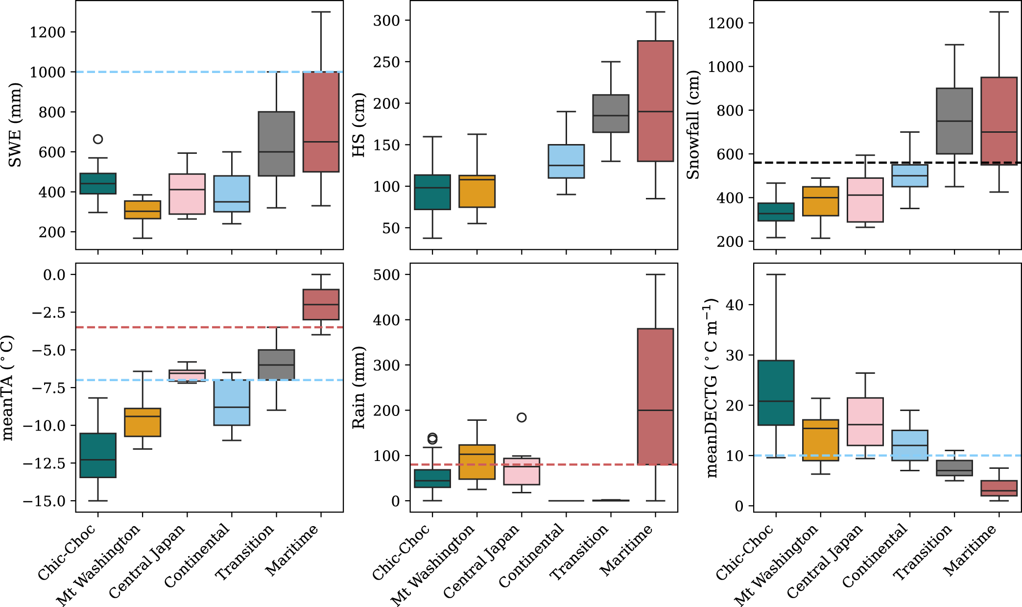
Figure 5. Box plot with all the Mock and Birkeland Reference Mock and Birkeland(2000) climate classification including Continental, Intermountain/Transition and Coastal/Maritime, for a international comparison with the Chic-Chocs dataset, Mount Washington (1180 m a.s.l) from Meloche Reference Meloche2019, Central Japan (Nishikoma 1900 m a.s.l) from Ikeda and others Reference Ikeda, Wakabayashi, Izumi and Kawashima(2009). The box corresponds to the 25th and 75th percentile and the whiskers correspond to the 10th and 90th percentile. The dashed lines represent the classification threshold of Mock and Birkeland Reference Mock and Birkeland(2000), for maritime (red), continental (blue) and transition (black).
3.2. Snow grain type
We compared the frequency of the grain types simulated in SNOWPACK using CRCM6 model with snow profile observations from 2015 to 2018. Figure 6a shows a discrepancy between observations and the simulated data. SNOWPACK tends to simulate MF more frequently than they are observed. Conversely, the simulation results seem to underrepresent DF. The presence of rounded grains (RG) and PP is similar between the simulation from the model chain CRCM6/SNOWPACK and the observations. The FC are more often observed in the snow profiles, but the FCxr are more frequent in the simulation from the model chain CRCM6/SNOWPACK. However, these grain types are similar and represent a similar transformation process in the snow cover. Finally, DH was more frequent in the snow profiles. Despite the differences between the simulations and the observations, the model chain CRCM6/SNOWPACK is relevant to retrieve the seasonal snow grain type distribution (Fig. 7).
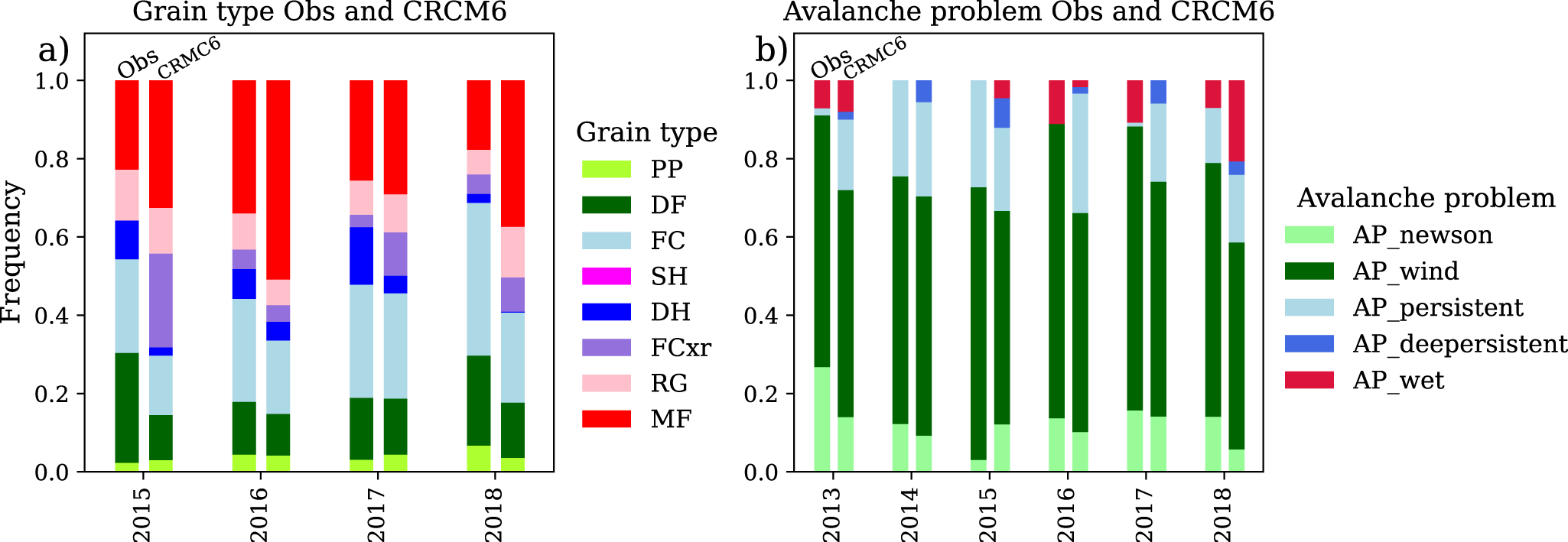
Figure 6. Comparison of the observations vs the simulated (CRCM6/SNOWPACK) for (a) snow grain type distribution and (b) avalanche problem frequency. The left barplot is the observations from Avalanche Québec and the right barplot is the climate simulation CRCM6 dataset. The avalanche problem types are the following: new snow avalanche problem (AP_newsnow), wind slab avalanche problem (AP_wind), persistent avalanche problem (AP_persistent), deep persistent avalanche problem (AP_deepersistent) and wet avalanche problem (AP_wet).
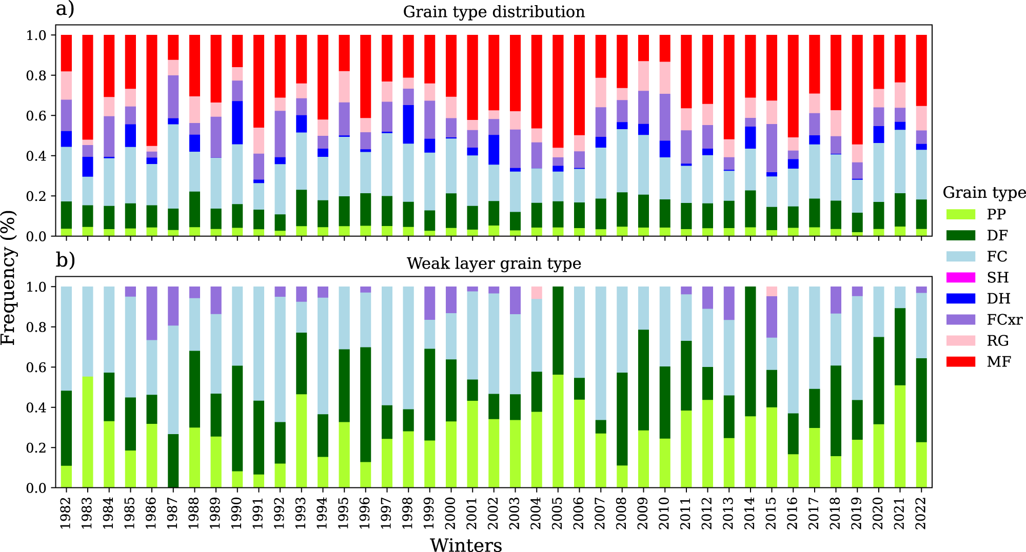
Figure 7. Snow grain type distribution over the 40 winters period with (a) snow grain type distribution of the whole snow cover each winter from December to the end of March and (b) the snow grain type distribution of the weak layer assessment for each winter (natural instability).
The snow grain type distribution was retrieved from the 40 year simulated snow cover to get an overview of the temporal variability in the metamorphic process of the study area. First, the snow grain type shows that MF are predominant in the snow cover from December to the end of March (Fig. 7a). The second most frequent grain type is rounding faceted grains (FC). However, Fig. 7a shows that there is a temporal variability between winters, with some winters having more FC than MF. The third and fourth most abundant grain types were faceted crystals (FCxr) and RG. The presence of these two grain types was quite variable between winters, sometimes with more FCxr than RG and sometimes vice versa (Fig. 7a). SH was not present in the snow cover during the entire 40 year period, from 1982 to 2022. Overall, the 40 year period of seasonal grain type distribution demonstrated different dominant metamorphic processes that should impact the dominance of specific avalanche problem types (i.e. persistent vs wet avalanche problem type).
The snow grain type distributions are different if looking at critical weak layers from the avalanche problem assessment (Fig. 7b). The three most common weak layer grain types are PP, DF and FC. Like the overall grain type assessment, the most frequent weak layer grain type was not the same from winter to winter, where sometimes DF and PP were more frequent over FC, and in some other winters the opposite occurs where FC was more frequent. It is important to note that this assessment is based on a weak layer with natural instabilities, and the frequency might change with including skier triggering. Some winters also had the FCxr in the weak layer assessment, and two winters had few weak layers with RG as a grain type. It is important to note that during the simulated 40 year period, neither DH nor SH was present in the critical weak layers, as well as in the snow pits of Avalanche Québec.
To explore the ‘typical’ stratigraphy of the study area, two examples of simulated snow profiles (south facing with 38∘ slope angle) for two winters that were classified as Maritime and Continental are presented in Fig. 8. The ‘continental’ winter of 2018 included a large rain event on 13 January (35 mm), which initiated a wet instability cycle for the next 10 days (Fig. 8a). After this event, however, colder conditions returned, with HSs continuing to increase with several layers of FC, up to a maximum HS of 240 cm. These cold conditions persisted until the end of March. The ‘maritime’ winter of 2021 had a large rain event (25 mm), which occurred on 25 December with a thinner snow cover (43 cm) and caused the snow cover to melt almost completely (Fig. 8b). The rain event delayed snow accumulation, resulting in a shallower snow cover compared to the continental winter of 2018. Despite the difference in amount and timing of the rain event in both winters, the resulting stratigraphy was quite similar and more representative of a continental snow cover with a thick melt-freeze crust in the basal layers, with FC above and DF/PP at the surface. The rains at the end of March were the main cause of this so-called maritime winter. This sequence of meteorological events creating different snow layers leads to a specific type of avalanche problem during the winter. In the following section, the winters of 2018 and 2021 are described in more detail in terms of avalanche problem type.

Figure 8. Seasonal stratigraphy and avalanche problem type from the snow cover model output for (a) an example Continental winter in 2018 and (b) an example of a stratigraphy during the Maritime winter of 2021. New snow avalanche problem (AP_newsnow), wind slab avalanche problem (AP_wind), persistent avalanche problem (AP_persistent), deep persistent avalanche problem (AP_deepersistent) and wet avalanche problem (AP_wet).
3.3. Avalanche problem type
3.3.1. Continental vs Maritime winter
Figure 8 shows the timing of avalanche problem types during the continental winter of 2018 and the maritime winter of 2021. The continental winter of 2018 had a significant amount of natural instabilities, with significant storms producing AP_newsnow, AP_wind, AP_persistent and AP_deepersistent throughout the whole season. The persistent problems (AP_persistent/AP_deepersistent) were more concentrated at the beginning of the winter (December), i.e. before the rain event of 13 January removed the persistent weak layers. Surprisingly, the continental winter had more wet-snow instabilities (AP_wet) despite having less total rainfall during the winter (50 mm) compared to the maritime winter (93 mm). The maritime winter of 2021 had persistent problems concentrated toward the end of the winter in January, February and March. Regarding the avalanche problem type, the difference between the ‘maritime’ and the ‘continental’ winter was not significant and does not correspond to the definition of a maritime winter (more precipitation, less or no AP_persistent/AP_deepersistent).
3.3.2. Observations vs simulations
We compared the seasonal frequency of predicted avalanche problem types from Avalanche Québec with those derived from snow cover modeling. In both cases, the most common avalanche problem type was wind slab avalanche problem (AP_wind) (Fig. 6b). Avalanche Québec generated slightly more AP_winds than the simulation from the CRMC6/SNOWPACK model chain. New snow problems (AP_newsnow) were more frequent compared to the simulation except for the winter of 2015. Conversely, the persistent problem type (AP_persistent) was also more frequent in the simulation compared to the Avalanche Québec forecast. Thus, AP_newsnow and AP_wind were underestimated and AP_persistent/AP_deepersistent were overestimated by the CRCM6/SNOWPACK model chain. The winters of 2016 and 2017 were the most different between the simulation and the forecasts of Avalanche Québec, with no AP_persistent/AP_deepersistent and AP_wet (Avalanche Québec) compared to more AP_persistent/AP_deepersistent and almost no AP_wet (CRCM6/SNOWPACK). The wet avalanche problem type (AP_wet) was the most variable between simulation and forecast. The deep persistent problem type (AP_deepersistent) was never forecasted by Avalanche Québec. These results show the systematic error or difference between the simulation and the forecast of the avalanche problem type, but we have to keep in mind that the significant differences could be related to the difference between the forecast guidelines (Avalanche Québec) and the numerical model (CRCM6/SNOWPACK).
3.4. 40 year period
Figure 9a shows the distribution of natural avalanche problem types that have occurred in our study area over the last 40 years. Four different avalanche problem types were present in the region, with the wind slab avalanche problem type (AP_wind) being the most prevalent in the region. The second most frequent problem type was the persistent problem type (AP_persistent) with an average of 13 days per winter and the deep persistent problem type (AP_deepersistent) with an average of 3 days per winter. The wet avalanche problem type (AP_wet) was not present every winter, with an average of 3.5 days/winter on a virtual northern aspect and 4.1 days/winter on a virtual southern aspect (more solar radiation) (Fig. 8). The second least frequent problem type was the new snow problem type with an average of 7 days per winter.
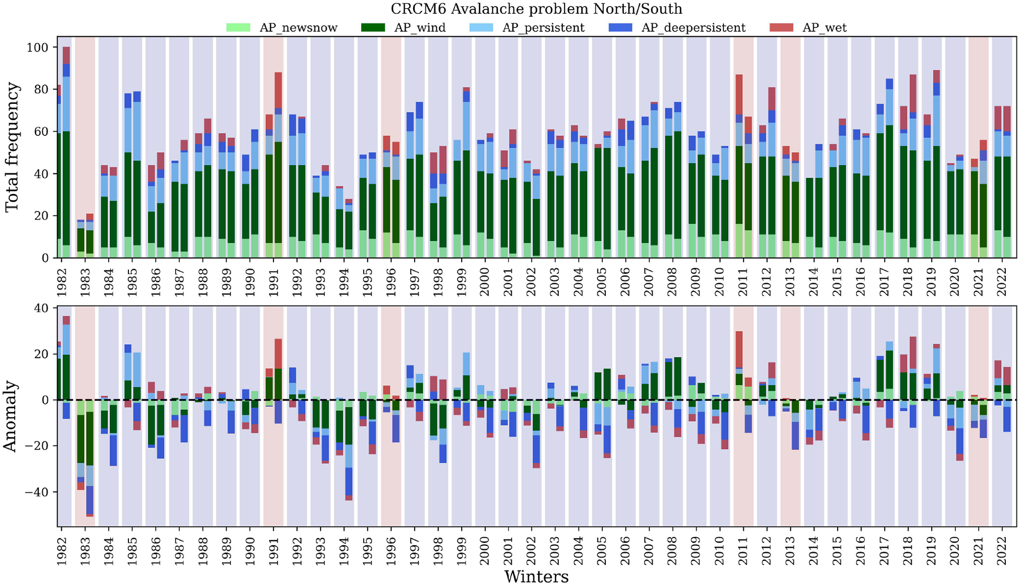
Figure 9. Avalanche problem distribution for the winter 1982 to 2022, with the north aspect on the left barplot and the south face on the right barplot. (a) Number of days where the problem type was issued and (b) the anomaly from the mean of the 40 year period. The blue colored background are winters classified as continental and the red is maritime. The avalanche problem types are the following: new snow avalanche problem (AP_newsnow), wind slab avalanche problem (AP_wind), persistent avalanche problem (AP_persistent), deep persistent avalanche problem (AP_deepersistent) and wet avalanche problem (AP_wet).
Figure 9b shows anomaly over the 40 year period, with the colored background representing the classification by the Mock and Birkeland Reference Mock and Birkeland(2000) algorithm. The distribution of avalanche problems does not seem to be different for the maritime winters. The winters of 1991, 2011 and 2018 had the most AP_wet anomalies of the dataset, but the winters of 1991 and 2011 were classified as maritime and the winter of 2018 was classified as continental. However, other maritime winters appear to be the same as other continental winters without specific anomalies, such as the winters 1996, 2013 and 2021 (Fig. 9b). These results indicate a possible limitation of the Mock and Birkeland Reference Mock and Birkeland(2000) algorithm and that the frequency of the seasonal avalanche problem type can give a different perspective on what could be a ‘maritime’ winter.
3.5. Clustering analysis
To get a new perspective on snow and avalanche climate classification, we clustered the avalanche problem types. The result of the Silhouette analysis shows that two clusters were the most significant for classifying the northern and southern simulations for the 40 winters, with an average Silhouette score of 0.25 and a Calinski–Harabasz score of 27.3. In close second, three clusters were also significant, with a Silhouette score of 0.24 and a Calinski–Harabasz score of 25.9. The remaining number of clusters (4, 5, 6, …, 10) had decreasing Silhouette and Calinski-Harabasz scores. Figure 10 shows the two and three clusters on a transformed dataset using PCA to visually represent the clustering. The two clusters of Fig. 10a and b can be compared to maritime and continental winters of the Mock and Birkeland Reference Mock and Birkeland(2000) algorithm. However, the seven maritime winters were in both clusters (two in the blue and five in the red) (Fig. 10). According to the vector variables of the PCA in Fig. 10c, the red cluster was characterized by more AP_wet and early AP_wet onset date (December and January). By opposition, the blue cluster had more instabilities with all dry avalanche problem types and a late AP_wet onset date later in April (not in the analysis). These two clusters were quite different from the classic maritime/continental, with the blue cluster having more dry avalanche problems (AP_newsnow, AP_wind, AP_persistent/AP_deepersistent). The only major difference between north and south aspects was that more AP_newsnow were simulated on northern aspects, and surprisingly, there was no significant difference in AP_wet or AP_wet onset date between aspects.
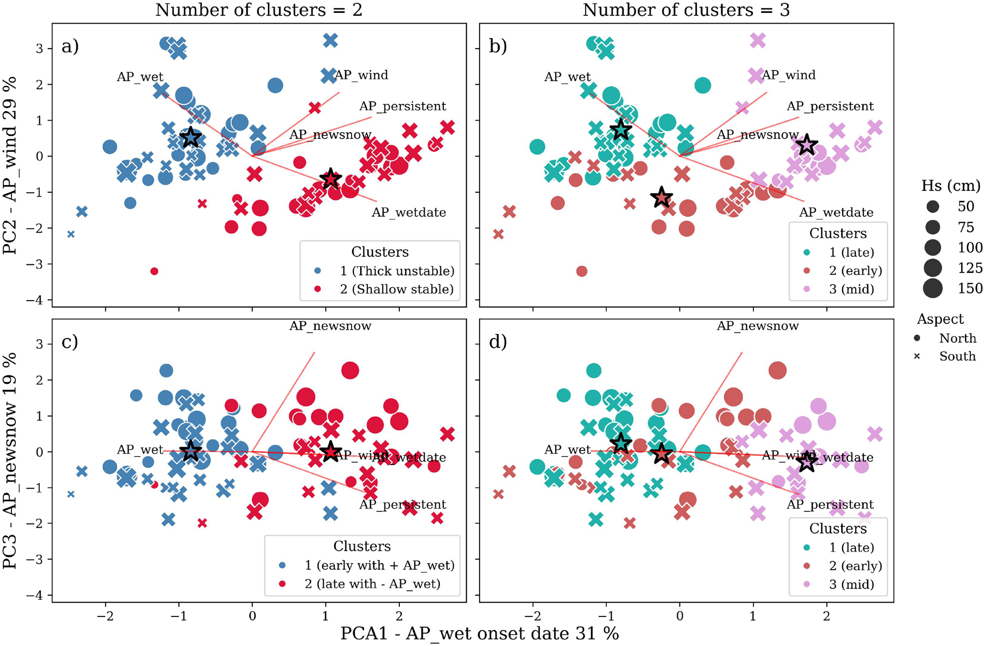
Figure 10. K-means clustering with two and three clusters. The clusters are shown in relation to the principal component 1 (AP_wet onset date 31%), principal component 2 (AP_wind day 29%) and the principal component 3 (AP_newsnow 19%). The red vectors represent their contribution (variance explained) along the three principal components. The stars represent the centroids of the clusters. South aspect simulations are represented by cross and north aspect simulations are represented by circles. The clustering with two clusters (a) and (c) demonstrates a new classification where winters were classified with a thick snow cover and unstable conditions and other winters with shallow snow cover and stable conditions. The clustering with three clusters (b) and (d) demonstrates a different classification with an early, mid and late AP_wet onset date.
The three clusters that resulted from the analysis are presented in Fig. 10b and d. The first cluster (red) was characterized by more AP_wet and early AP_wet onset date mostly in December. The second cluster (pink) was characterized by lowest AP_newsnow, AP_wind and AP_persistent/AP_deepersistent with early to mid AP_wet onset date (January). The third cluster (turquoise) had the latest AP_wet onset date (April) and the lowest number of AP_wet relative to our dataset.
To compare our clusters with another region, we present in Fig. 11 our three clusters compared to the data of Reuter and others Reference Reuter, Hagenmuller and Eckert(2023), who clustered the avalanche problem type of the French Alps. We compared the three cluster centroids of this present study with the four centroids found in the French Alps. Two clusters had similar centroids between both studies, which were the pink clusters (cluster 1 and 5) and the turquoise-green clusters (cluster 3 and 8) (Fig. 11). The pink cluster in both studies had mid-season AP_wet onset date around February with a relatively low number of days with a persistent avalanche problem with 10 or less, and around 5 days of new snow problems, and the lowest number of days of wind slab problem. This cluster was observed, in the study of Reuter and others Reference Reuter, Hagenmuller and Eckert(2023), in the front ranges of the French Alps, in regions like Vercors and Chartreuse, which classify mostly as ‘maritime’ according to the Mock and Birkeland Reference Mock and Birkeland(2000) algorithm. The remaining cluster of this study (cluster 2 in red) does not fit with the other clusters from the Alps. Figure 11b and c show the red cluster with a AP_wet onset date early during the season in December, which no cluster had such an early AP_wet onset date in the Alps. In terms of AP_newsnow and AP_persistent days, the red cluster from our study was similar to the green cluster of Reuter and others Reference Reuter, Hagenmuller and Eckert(2023).
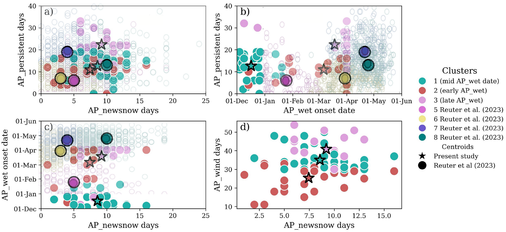
Figure 11. Three clusters of this study (solid circles) presented in comparison with the cluster centroids (stars) and the data in transparency of the study of Reuter and others Reference Reuter, Hagenmuller and Eckert(2023) (disks). The pink cluster of Reuter and others Reference Reuter, Hagenmuller and Eckert(2023) represents a cluster with low AP_newsnow, low AP_persistent and a early AP_wet onset date before March. The green cluster of Reuter and others Reference Reuter, Hagenmuller and Eckert(2023) represents a cluster with high AP_newsnow, mid AP_persistent and late AP_wet onset date after April. The yellow cluster of Reuter and others Reference Reuter, Hagenmuller and Eckert(2023) represents a cluster with high AP_newsnow, low AP_persistent and mid AP_wet onset date around April. The purple cluster of Reuter and others Reference Reuter, Hagenmuller and Eckert(2023) represents a cluster with low AP_newsnow, high AP_persistent and late AP_wet onset date around mid-April.
4. Discussion
4.1. Limitations of climate simulations
This research provides an in-depth analysis of the snow and avalanche climate of the Chic-Chocs region, located in the northeastern Appalachian range in Canada. Through the use of climate indicators, snow grain types and avalanche problem types, we aim to provide a comprehensive understanding of snow processes leading to avalanches in the region. Our dataset, derived from 40 years of CRCM6 climate simulation over North America, serves as a robust basis for simulating snow stratigraphy and avalanche problem types over this time period. This approach identifies snow cover characteristics relevant for avalanche situations. The use of snow cover modeling provides a new perspective on snow and avalanche climates in the region and complements the data available for snow and avalanche climatology.
Despite providing a significant temporal perspective, the model chain CRCM6-SNOWPACK simulations we show have inherent bias stemming from the climate data or the snow cover simulations. To evaluate the performance of the CRCM6-SNOWPACK model chain, we present a comparison between observations and the simulation for the climate indicators (Table 1), snow grain types (Fig. 6a) and avalanche problem types (Fig. 6b). The uncertainties in the climate indicators and their classification, as described by Mock and Birkeland Reference Mock and Birkeland(2000), are mainly due to the classification of precipitation as rain or snow in both meteorological observations and CRCM6/SNOWPACK simulation (Fig. 3). For example, the winter of 2013 was classified as continental in the meteorological observations but as maritime using the CRCM6 simulations, highlighting the discrepancies between the observations and the simulations with respect to precipitation events. Additional uncertainties arise from the precipitation gauge at the weather station, where snow accumulation on top of the gauge can prevent accurate measurement during rain.
A scale issue between the resolution of the climate model (12 km) and the point scale weather observations can certainly cause and explain discrepancies in our results. While the proposed correction of the CRCM6 model improved the performance of the SNOWPACK model output, notable discrepancies and underestimations persist in certain cases. Additionally, a key limitation of this methodology is that by re-accumulating the positively adjusted hourly snowfall, the processes of compaction and melt remain unchanged, even though they should be affected. Moreover, the approach of using the median underestimation of each precipitation intensity class to correct the data introduces potential bias. If the climate model completely misses certain precipitation events, the calculated median underestimation may be artificially inflated, leading to an overcorrection of the data. Finally, a more detailed analysis of precipitation underestimation patterns is necessary to further enhance the accuracy of the CRCM6 model in this region.
4.2. Limitations of SNOWPACK modeling
The SNOWPACK model, in the current settings used in this study, has limitations that could affect the stratigraphy and thus the resulting uncertainty for avalanche problem types. As discussed in the previous section, the classification between rain and snow is also a limitation of the threshold used in the SNOWPACK model. We chose to use the default rain/snow threshold of 1.2∘C, which was empirically determined based on measurements in Switzerland. Bellaire and Jamieson Reference Bellaire and Jamieson(2013) simulated the snow cover in western Canada using numerical weather prediction of 15 km spatial grid and tested different rain/snow thresholds to detect melt-freeze crust formation in Rogers Pass, Canada. The default threshold of 1.2∘C had the lowest probability of detection compared to other thresholds closer to 0∘C, which had a higher probability of detecting melt-freeze crusts. However, Madore and others Reference Madore, Fierz and Langlois(2022) simulated the snow cover in Rogers Pass based on a meteorological station and demonstrated that a threshold of 1.4∘C was better at simulating both melt-freeze crusts with an accurate estimation of the HS. They also point out that this threshold was only found for the winter of 2018–19, and that different winters could have a different threshold based on a different meteorological event (i.e. thermal inversion) or even different snow and avalanche climates (Bellaire and Jamieson, Reference Bellaire and Jamieson2013). This contrast between the results of Bellaire and Jamieson Reference Bellaire and Jamieson(2013) and Madore and others Reference Madore, Fierz and Langlois(2022) supports the argument that this threshold could be different depending on the meteorological context. Although the selected rain/snow threshold has been evaluated locally, a comprehensive study across the northern hemisphere has highlighted the spatial differences in rain/snow thresholds along longitudes (Jennings and others, Reference Jennings, Winchell, Livneh and Molotch2018). The research indicates that continental climates generally have higher temperature thresholds (around 2 and 3∘C), whereas maritime climates display lower thresholds between 1 and 0.5∘C (Jennings and others, Reference Jennings, Winchell, Livneh and Molotch2018). For the Chic-Chocs, it has been shown that both continental and maritime influences are present in the study area, future work should focus on assessing the sensitivity of the rain/snow threshold to simulate specific melt events and melt-freeze layers in the Chic-Chocs.
The second limitation is related to the density of the snow precipitation in both CRCM6 and SNOWPACK. Even with applying a precipitation correction of Imbach and others Reference Imbach, Gauthier and Langlois2024, the estimation of snow precipitation (SWE) had an average error of 54.5 mm and MRE of 17% (Fig. 3). This poor estimation of snow precipitation led to an underestimation of the HS (Fig. 2). The estimation of SWE and underestimation of HS could indicate a problem with the density of the new snow or the densification of the entire snow cover. We used the Bellaire and Jamieson Reference Bellaire and Jamieson(2013) new snow density parameterization, which is an empirical fit of new snow density based on several weather variables such as air temperature, wind speed and relative humidity (Lehning and others, Reference Lehning, Bartelt, Brown, Russi, Stockli and Zimmerli1999). This parameterization is an empirical fit based on measurements in Switzerland but may not be applicable in eastern Canada. Future work should investigate a different or new parameterization of new snow density that is better suited to the snow and avalanche climate of eastern Canada. Despite introducing uncertainty in individual winter events, the CRCM6-SNOWPACK model chain was in agreement at representing the seasonal average of climatic indicators, snow grain type and avalanche problem type that represent well the snow and avalanche climate of the region.
4.3. International comparison
We applied the Mock and Birkeland Reference Mock and Birkeland(2000) algorithm to 40 winters using climatic indicators derived from the CRCM6/SNOWPACK model chain. Thirty-three of the forty winters were classified as continental, and the remaining seven winters as maritime (Fig. 4). Shandro and Haegeli Reference Shandro and Haegeli(2018) applied the Mock and Birkeland Reference Mock and Birkeland(2000) algorithm to three areas in western Canada: the Coastal Mountains (i.e. Whistler), the Columbia Mountains (i.e. Revelstoke) and the Rocky Mountains (i.e. Banff). Comparing our snow and avalanche climate classification results with the three areas in western Canada (Shandro and Haegeli, Reference Shandro and Haegeli2018), each of these three areas never had continental and maritime winters classified in the same area. The Coastal Mountains only had maritime and transitional winters. The Columbia Mountains had mostly transitional winters with some continental and maritime winters. The Rocky Mountains only had continental winters and some transitional winters. Our study area is not similar to western Canada, which had continental winters with some maritime winters. From the perspective of seasonal avalanche problem frequency, the Chic-Chocs region exhibits a distribution with around 10% of wet-snow problem types, around 10–20% persistent avalanche problem types, and the remaining is mostly wind slab and new snow problem types (Fig. 9). This seasonal avalanche problem type frequency was similar to the Coastal Mountains (mostly maritime winters) and the Columbia Mountains (mostly transitional winters). Surprisingly, the Rocky Mountains had mostly continental winters like our study area, but the persistent problem type was more present around 60–70%, compared to 10–20% in the Chic-Chocs (Fig. 9).
If we compared the climatic indicators of Mock and Birkeland Reference Mock and Birkeland(2000) algorithm with the three classic western regions in the United States, our study area shares similarities with continental regions for all meteorological variables except rain (Fig. 5). Other regions of the world, such as Mount Washington and the central Japanese Alps, exhibit the same pattern of low snowfall, cold air temperatures and significant precipitation during winter (Fig. 5). This suggests that the Chic-Chocs are also influenced by climate factors typical of the continental and maritime snow and avalanche climates, resulting in snow and avalanche climate characteristics that do not fit neatly into established classifications of western North America. The sequence from cold temperatures to significant rain is a distinguishing feature that sets these regions apart from classic snow and avalanche climates of western North America. This dual influence results in snow cover that exhibits characteristics of both continental and maritime climates, such as the presence of FC and layers of ice due to rain-on-snow events. These mixed characteristics between continental and maritime winters defined the specific climatic and snow cover conditions of regions such as the Chic-Chocs, Mount Washington and the Central Japanese Alps.
The snow grain type distribution and climatic conditions of the study area can be compared with those studied in Svalbard, Norway (Eckerstorfer and Christiansen, Reference Eckerstorfer and Christiansen2011). Both snow covers are cold and relatively thin (≈1–1.5 m), dominated by temperature gradient metamorphism processes. These regions experience basal instability and FC due to cold winter temperatures and are also affected by maritime depressions that bring warm air and rain, causing ice/melt freeze stratification in the snow cover. Similar to Svalbard, our results showed that the Chic-Chocs region has snow grain types characteristic of both a continental climate (facet and DH) and a maritime climate (ice/melt-freeze layering) (Figs 6 and 7). Snow and climate data revealed two major snow and avalanche climate components: a cold snow cover combined with a maritime influence causing rain-on-snow events.
Ikeda and others Reference Ikeda, Wakabayashi, Izumi and Kawashima(2009) described two study areas in the Japanese Alps: the Japanese Coastal Mountains (Northern Japanese Alps) and the Central Japanese Alps. Their research shows similarities between the Central Japanese Alps and the Chic-Chocs region (Fig. 5). Both regions obtained similar snow and avalanche climate results using the Mock and Birkeland Reference Mock and Birkeland(2000) flowchart: primarily continental winters with some maritime winters (Ikeda and others, Reference Ikeda, Wakabayashi, Izumi and Kawashima2009). The criteria used for classification are also similar, with a continental winter characterized by a mean December temperature gradient (meanDECTG  $ \gt 10^{\circ}\mathrm{C}$) and a maritime winter characterized by rainfall (>80 mm) (Ikeda and others, Reference Ikeda, Wakabayashi, Izumi and Kawashima2009). The climatic conditions are similar, with cold air temperatures, low snowfall and significant precipitation (Fig. 5). The snow cover structures are comparable, showing a strong prevalence of FC and MF (Ikeda and others, Reference Ikeda, Wakabayashi, Izumi and Kawashima2009). The authors found that these characteristics did not fit any of the three major snow and avalanche climate classifications, leading them to propose a new classification for the Central Japanese Alps: the Rainy Continental snow and avalanche climate. This new classification is defined by the following specific characteristics (Ikeda and others, Reference Ikeda, Wakabayashi, Izumi and Kawashima2009):
(1) A relatively thin snow cover and cold air temperatures, similar to continental snow and avalanche climate regions.
(2) Heavy rainfall, comparable to or exceeding that of maritime snow and avalanche climate regions.
(3) Persistent structural weakness caused by FC and DH, similar to continental snow and avalanche climate regions.
(4) The dominance of both FC and wet grains.
4.4. Snow and avalanche climatology
Similar to Ikeda and others Reference Ikeda, Wakabayashi, Izumi and Kawashima(2009), our results suggest that the snow and avalanche climate of the Chic-Chocs does not fit into the three traditional snow and avalanche climate classifications. Historically, the Chic-Chocs region has been classified as a maritime snow climate according to the Sturm and others Reference Sturm, Holmgren and Liston(1995) global classification, which is based solely on climatic variables such as temperature and precipitation without considering snow cover or avalanche regimes (Sturm and others, Reference Sturm, Holmgren and Liston1995). Other authors have used the term Cold Maritime to describe the winter climate of the region (Fortin and others, Reference Fortin, Hétu and Germain2011; Gauthier and others, Reference Gauthier, Germain and Hétu2017).
The Chic-Chocs region shares similarities with several regions around the world, such as Mount Washington and the Central Japanese Alps (Fig. 5). All of these regions are influenced by cold air masses from the continent and low-pressure cells from the ocean. These specific influences of both continental and maritime low-pressure cells have previously been observed for the northeastern coast of the United States (Karmosky, Reference Karmosky2007; Perry and others, Reference Perry, Konrad, Hotz and Lee2010). This contrasts with the coastal mountain ranges of the northwestern United States, which are primarily influenced by maritime low-pressure cells. The four characteristics mentioned above for the Rainy Continental classification of the Central Japanese Alps are identical to those observed for the Chic-Chocs. The term ‘Rainy Continental’ proposed by Ikeda and others Reference Ikeda, Wakabayashi, Izumi and Kawashima(2009) expresses both continental and maritime influences, similar to a transitional snow and avalanche climate. However, the term Rainy Continental could be a better fit for insular, peninsular or northeastern continental regions than any of the three major snow and avalanche climates developed for the larger mountain ranges of the western United States.
Recently, Reuter and others Reference Reuter, Hagenmuller and Eckert(2023) characterized snow avalanche climate regions in the French Alps by occurrences of avalanche problem types relevant for natural release. They applied the traditional snow and avalanche climate classification of Mock and Birkeland Reference Mock and Birkeland(2000) and compared the results with a snow avalanche climatology based on a clustering analysis of avalanche problem type occurrences. Their analysis revealed four clusters defined by the number of days with persistent problems, the number of days with new snow problems and the onset date of wet-snow problems. These three factors lead to a combination of seven possibilities, four of which they observed in the French Alps, with potentially three more based on their criteria. Based on our clustering analysis, two of our clusters were similar to two of the clusters observed in the French Alps (Fig. 11). One cluster was similar to the one in the French Alps and has an average wet-snow activity onset date around February with a relatively low frequency of persistent weak layers (of around 8 days per season) and about 6 days with new snow problems. This cluster was observed in front-range regions on the western flank of the French Alps. A second cluster, similar to the Mont Blanc or the Beaufortain range in the French Alps, had a late wet-snow onset date around the end of April or later, around 13 days with persistent weak layers and 10 days with new snow problems per season. Our study revealed another cluster with a very early wet-snow onset date in December, but with similar frequencies of persistent and new snow problems (Figs 10 and 11).
Regarding climate change, Eckert and others Reference Eckert(2024) and Mayer and others Reference Mayer(2024) reviewed the past and projected effects of climate change on avalanche activity. They found a significant decrease in dry snow avalanches relative to an increase in wet snow avalanches. Currently, more winters are characterized by dry snow situations, such as new snow, wind slabs and persistent problem types, compared to wet-snow problem types. However, as shown by Eckert and others Reference Eckert(2024), these proportions could change toward more situations with wet-snow relative to dry-snow avalanche problems. Giacona and others Reference Giacona(2021) observed an upslope shift of avalanche activity, where low altitude mountains saw a reduction in the number and the period of avalanches. This finding suggests that clusters with late onset dates (April) of wet-snow avalanche problems are likely to be affected or disappear in favor of the other two clusters with a mid-season (February) and early wet-snow onset date (December). Today’s Chic-Choc snow and avalanche climate may correspond to the projection of snow and avalanche climates in other regions, as the Rainy Continental may be the new Continental.
4.5. Perspective
Building on the framework developed by Reuter and others (Reference Reuter2022, Reference Reuter, Hagenmuller and Eckert2023), this study details and characterizes the snow and avalanche climate of the Chic-Chocs range, located in the northeastern Appalachian Mountains of North America. The implementation of the avalanche problem type, derived from 40 winters of SNOWPACK simulations, provided a unique perspective to describe the snow and avalanche climate of the area. As suggested by Shandro and Haegeli Reference Shandro and Haegeli(2018) and Reuter and others Reference Reuter, Hagenmuller and Eckert(2023), using the avalanche problem type introduces a new perspective to propose new classifications for regions that differ from the three conventional snow and avalanche climates found in western North America. Unlike the geographic clustering study of Reuter and others Reference Reuter, Hagenmuller and Eckert(2023), our approach was temporal, aiming to identify different ‘types’ of winters that the region may experience. Figure 10b and d illustrate a clustering into three categories over the 40 winters, differing from the continental and maritime ‘types’ of winters by primarily using the avalanche problem type. This type of research opens the possibility to characterize the snow and avalanche climate where field data are not available. The ERA5 climate model of the European Centre for Medium-Range Weather Forecasts (ECMWF), coupled with the SNOWPACK simulation and the method of Reuter and others Reference Reuter(2022), represents a new potential framework to analyze new regions that aim to create a historic record of avalanche problem types and tailor a forecasting system based on their climate.
5. Conclusion
This study provides a comprehensive analysis of the snow and avalanche climate in the Chic-Chocs region of the Gaspé Peninsula, as part of the northeastern Appalachians in eastern Canada. Using a variety of methods and data sources, including meteorological observations, snow grain type distributions and avalanche problem types, we provide a detailed characterization of the region’s specific snow and avalanche climate.
The snow and avalanche climate classification results, based on the Mock and Birkeland Reference Mock and Birkeland(2000) flowchart, indicate a predominantly continental climate with occasional maritime winters. This finding contrasts with the more traditional snow and avalanche climate observed in western North America, highlighting the specificity of the Chic-Chocs region. Our comparison with similar regions around the world, such as Mount Washington and the central Japanese Alps, revealed patterns of low snowfall, cold air temperatures and significant rain precipitation. This similarity suggests that the Chic-Chocs, like these other regions, do not fit neatly into traditional classifications of continental, maritime or transitional snow and avalanche climates. These conditions result in a snow cover structure characterized by both continental and maritime elements, such as FC and ice/melt freeze layers.
The inclusion of avalanche problem types derived from 40 winters of snow cover simulations (CRCM6-SNOWPACK) provided seasonal patterns of natural snow instability mostly dependent on the month where the wet-snow problem type occurs. We were able to compare our results with another study in the French Alps and discuss a classification/cluster exclusively around avalanche problem types, shifting from the traditional climate-based description. This study highlights the potential of snow cover modeling and avalanche problem type methodology to improve our understanding and classification of snow and avalanche climates, ultimately contributing to improved avalanche forecasting and risk management in regions with similar complex dynamics. Finally, in our broader perspective of climate change, where rain and wet-snow problem type may become more common for continental regions around the world, the Rainy Continental of the Chic-Chocs may be the new Continental around the world.
Acknowledgements
We would like to thank Dominic Boucher, Julie Leblanc and Jean-Pierre Gagnon from Avalanche Québec for providing us with their meteorological and forecast dataset. We want to acknowledge them for all the discussions based on their 20 years of expertise of the Chic-Chocs area. We also want to thank the Centre pour l’étude et la simulation du climat à l’échelle régionale (ESCER), specifically Philippe Gachon and Clémence Benoit for providing us the CRCM6 simulations.


 Open access