


1. Introduction
The results of an experimental investigation into levitating spheres on a vertical moving wall covered with a thin layer of viscous liquid are presented. Levitation is established by the lubrication layer, which forms in the viscous fluid between the sphere and the moving wall. One configuration comprises a semi-rigid plastic belt oriented vertically and passing through a bath of very viscous fluid, resulting in a thin layer being formed on the belt. The second experiment involves a thin viscous layer formed on the inside of a rotating cylinder where the axis of the cylinder is horizontal. The issue of suspending particles in viscous layers is of general, practical interest with applications in industrial processes such as the creation of antireflective coatings as investigated by Prevo, Kuncicky & Velev (Reference Prevo, Kuncicky and Velev2007), the spreading of colloidal particles in thin fluid films as studied by Kao & Hosoi (Reference Kao and Hosoi2012) and the dispersion of subsurface pollutants through a partially saturated underground environment as investigated by Veerapaneni, Wan & Tokunaga (Reference Veerapaneni, Wan and Tokunaga2000).
At the fundamental level, the motion of the sphere involves a lubrication layer between its surface and the wall. Modelling the interaction between the lubrication layer and the nearby free surface of the film is a considerable theoretical challenge as discussed by Marshall (Reference Marshall2014). In all experiments with a plane wall and in the majority of studies where the inside of a horizontal rotating cylinder is used, the contact region is often nearly circular between the sphere and the film. This leads to two tracks in the film downstream of the sphere. The tracks are initiated at the edge of the circle of contact. They also wrap around the sphere so that the geometry of the intersection between the sphere and the film is complex with flattened regions on the circle (see figure 9 a). However, another state exists for the sphere on the film inside a cylinder. In this case a single track is left behind by the sphere in the film. It is observed that the contact region between the sphere and the film is almost a perfect circle (see figure 9 b) and this allows mathematical progress to be made (Ockendon et al. Reference Ockendon, Ockendon and Mullin2024). Good agreement between theory and experiment is found in this case for the dependence of the slip speed ratio on wall speed. A systematic experimental investigation of the motion of spheres down inclined planes covered by a thin layer of very viscous fluid was performed by Bico et al. (Reference Bico, Ashmore-Chakrabarty, McKinley and Stone2009). They established that slip between the surface of the particle and the plane is an essential part of motion. A lubrication layer is formed between the two solid surfaces, but complexities introduced by the free surface and the coating of the sphere by the fluid make a full theoretical treatment of the problem challenging. However, they used dimensional analysis and included the physical properties of the fluids and the length scales involved to provide a framework that established an empirical scaling of the experimental data.
Our work builds on previous studies of viscous levitation of cylinders on vertical belts initiated by Eggers, Kerswell & Mullin (Reference Eggers, Kerswell and Mullin2013), extensively developed in a theoretical, numerical and experimental investigation by Dalwadi et al. (Reference Dalwadi, Cimpeanu, Ockendon, Ockendon and Mullin2021). Closely relevant theoretical and experimental results for rectangular blocks are provided by Mullin, Ockendon & Ockendon (Reference Mullin, Ockendon and Ockendon2020) .
The problem we address here concerns the motion of spheres over a range of diameters on a moving wall that is covered with layers of very viscous fluid. We find a systematic dependence of the results on control parameters, despite the complexities of the problem, such as free surfaces on the layer and the sphere, and the lubrication layer between the moving wall and the rotating ball. A qualitative difference is found between levitation with a plane and curved surface. In summary, motion occurs at fixed locations, on the inside of a cylinder, with thresholds between qualitatively distinct types of motion. On the other hand, the motion in the planar case is most often transient, but balance can be achieved under particular conditions.
2. The experiments
2.1. Overview
Two sets of apparatus were constructed to investigate the levitation of spheres on viscous layers on a moving wall. In one, a vertical belt passes through a bath of viscous silicone oil and a sharp-edged metal scraper is used to create a uniform viscous layer of a specified depth. In the second experiment, a viscous layer is formed on the inside of a horizontal rotating glass cylinder, where a bath and centrally mounted scraper system is used to create viscous layers with a defined depth.
2.2. Fluids, spheres and parameters
The fluid used in most experiments is $13\,740\pm 140$
cSt silicone oil. The viscosity is measured using a falling ball viscometer. Some experiments are performed using silicone oils with viscosities of
$13\,740\pm 140$
cSt silicone oil. The viscosity is measured using a falling ball viscometer. Some experiments are performed using silicone oils with viscosities of $66\,000 \pm 660$
and
$66\,000 \pm 660$
and $1100\pm 12$
cSt. Silicone oils are the preferred choice of viscous fluid, since they readily wet surfaces and are more amenable to creating layers with a uniform thickness. Further preliminary experiments were conducted using concentrated syrups, but the results were found to be unreliable since the fluid tends to form puddles and does not wet the surfaces evenly.
$1100\pm 12$
cSt. Silicone oils are the preferred choice of viscous fluid, since they readily wet surfaces and are more amenable to creating layers with a uniform thickness. Further preliminary experiments were conducted using concentrated syrups, but the results were found to be unreliable since the fluid tends to form puddles and does not wet the surfaces evenly.
The experiments are carried out in a temperature-controlled laboratory where the temperature is set to $20 \pm 1\,^{\circ }\textrm {C}$
. The temperature of the silicone oil is monitored digitally. The density of silicone oils is
$20 \pm 1\,^{\circ }\textrm {C}$
. The temperature of the silicone oil is monitored digitally. The density of silicone oils is $970\pm 10$
kg m
$970\pm 10$
kg m $^{-3}$
and the surface tension is
$^{-3}$
and the surface tension is $21.5$
mN m
$21.5$
mN m $^{-1}$
.
$^{-1}$
.
The spheres ranged in size from $3$
to
$3$
to $15$
mm in radius
$15$
mm in radius $r$
and were made from the following materials: steel,
$r$
and were made from the following materials: steel, $ \rho =7800\pm 100$
kg m
$ \rho =7800\pm 100$
kg m $^{-3}$
; polypropylene,
$^{-3}$
; polypropylene, $\rho =898 \pm20$
kg m
$\rho =898 \pm20$
kg m $^{-3}$
; acetate,
$^{-3}$
; acetate, $\rho =1300\pm 20$
kg m
$\rho =1300\pm 20$
kg m $^{-3}$
; glass,
$^{-3}$
; glass, $\rho =2600\pm 30$
kg m
$\rho =2600\pm 30$
kg m $^{-3}$
; and rubber,
$^{-3}$
; and rubber, $\rho =1522\pm 25$
kg m
$\rho =1522\pm 25$
kg m $^{-3}$
. The Reynolds number
$^{-3}$
. The Reynolds number $ \textit{Re}$
is defined here as
$ \textit{Re}$
is defined here as $ {Uh}/{\nu }$
, where
$ {Uh}/{\nu }$
, where $U$
is the wall speed,
$U$
is the wall speed, $h$
is the depth of the viscous layer and
$h$
is the depth of the viscous layer and $\nu$
is the kinematic viscosity of the oil. Here, the Reynolds number is in the range between
$\nu$
is the kinematic viscosity of the oil. Here, the Reynolds number is in the range between $10^{-3}$
and
$10^{-3}$
and $ 10^{-4}$
and hence the flow can be considered as Stokesian. The capillary number
$ 10^{-4}$
and hence the flow can be considered as Stokesian. The capillary number $\textit{Ca}= {U\mu }/{\sigma }$
, which is the ratio of viscous forces to surface tension, ranges from
$\textit{Ca}= {U\mu }/{\sigma }$
, which is the ratio of viscous forces to surface tension, ranges from ${\sim} 0.3$
to
${\sim} 0.3$
to ${\sim} 70$
so that both forces are important. Finally, the Bond number
${\sim} 70$
so that both forces are important. Finally, the Bond number $Bo={\rho g r^2}/{\sigma }$
, which is defined to be the usual ratio of gravitational to surface tension forces multiplied by
$Bo={\rho g r^2}/{\sigma }$
, which is defined to be the usual ratio of gravitational to surface tension forces multiplied by $ \rho _{\textit{solid}} / \rho _{\textit{fluid}}$
, ranges from
$ \rho _{\textit{solid}} / \rho _{\textit{fluid}}$
, ranges from ${\sim} 0.3$
to
${\sim} 0.3$
to ${\sim} 300$
where the larger values correspond to steel spheres so that gravitational effects are greater.
${\sim} 300$
where the larger values correspond to steel spheres so that gravitational effects are greater.
3. The vertical belt experiment
A schematic diagram of the belt apparatus is given in figure 1(a) and a photograph of the details of the flow around the ball is given in figure 1(b). There is a circle of intersection between the sphere and the layer. Two symmetrically disposed ridges appear in the film downstream of the sphere, and these thicker ridges of fluid form tracks, which are also dragged around the rotating sphere. We refer to this as a two-track state, and these features are typical of all the experiments with spheres on a vertical belt. Specifically, the two-track state is the only one observed in the belt experiment, whereas both two-track and single-track states can coexist in the cylinder experiment as described below.

Figure 1. (a) Schematic diagram of the moving belt apparatus. The side view is shown on the left and the front view on the right. (b) A $15.8$
mm polypropylene sphere balanced on a
$15.8$
mm polypropylene sphere balanced on a $0.3$
mm layer. The two tracks are visible behind the sphere.
$0.3$
mm layer. The two tracks are visible behind the sphere.
The smooth vertical moving surface is provided by the outside of a steel-reinforced polyurethane internal combustion engine timing belt that is $375$
mm long and
$375$
mm long and $26.5$
mm wide. The part of the belt that forms the vertical moving wall is
$26.5$
mm wide. The part of the belt that forms the vertical moving wall is ${\sim} 150$
mm long. The belt is driven by one of a pair of
${\sim} 150$
mm long. The belt is driven by one of a pair of $38$
mm tooth pulleys that match the teeth on the inside of the belt. The drive is provided by a DC motor with a controlled feedback loop and the motor is connected to the drive pulley through either 6 : 1, 50 : 1 or 100 : 1 gearboxes. The particular gearbox selected depends on the density of the material of the sphere. In every case, the rotation rate of the drive is monitored using an optical shaft encoder, which produces
$38$
mm tooth pulleys that match the teeth on the inside of the belt. The drive is provided by a DC motor with a controlled feedback loop and the motor is connected to the drive pulley through either 6 : 1, 50 : 1 or 100 : 1 gearboxes. The particular gearbox selected depends on the density of the material of the sphere. In every case, the rotation rate of the drive is monitored using an optical shaft encoder, which produces $800$
pulses per revolution. The output of this device is measured using an electronic counter, and a calibration between this and the belt speed was established using a stopwatch to time a set number of rotations. The calibration is found to be linear for all three gearboxes.
$800$
pulses per revolution. The output of this device is measured using an electronic counter, and a calibration between this and the belt speed was established using a stopwatch to time a set number of rotations. The calibration is found to be linear for all three gearboxes.
The belt passes through a bath at the base of the apparatus. A scraper of the same width as the belt is used to set the film thickness. The scraper is held by two screws in slots at each end. The width of the gap between the scraper and the belt is set using metal shim plates. The thickness of the film is checked using a needle mounted on a micrometer head and observing the location where it first touches the surface of the oil using a travelling telescope. The location of the belt surface is determined by the slip of the clutch in the micrometer.
Uniform fluid layers of thicknesses in the range of $0.1$
to
$0.1$
to $0.75$
mm were used. Film drainage was not significant in the investigated range since the maximum drainage speed given by
$0.75$
mm were used. Film drainage was not significant in the investigated range since the maximum drainage speed given by $u_{drain}= {gh^2}/{2\nu }$
( where
$u_{drain}= {gh^2}/{2\nu }$
( where $g$
is gravitational acceleration,
$g$
is gravitational acceleration, $h$
is the layer thickness and
$h$
is the layer thickness and $\nu$
is the kinematic viscosity of the fluid) was an order of magnitude slower than the smallest belt speed. Hence, drainage effects are negligible and no significant variations in film thickness were found.
$\nu$
is the kinematic viscosity of the fluid) was an order of magnitude slower than the smallest belt speed. Hence, drainage effects are negligible and no significant variations in film thickness were found.
A viscous layer is formed on the belt by moving it through the silicone oil reservoir and passing through the scraper section at a fixed rate. The speed of the belt is then set to the required value and a sphere is placed on the belt. In the extreme case of a stationary belt, the action of surface tension causes the sphere to adhere to the viscous layer and it rolls down the belt. As the speed of the belt is increased, the rate of descent of the sphere reduces until a balance is achieved when the belt speed approximately matches the fall speed of the sphere. Further increases in the belt speed cause the sphere to move up the belt.
The main observations are of the rotation and translation speed of the spheres over a range of belt speeds. The rotation speed was estimated by timing $20$
crossings of a felt pen mark on the surface of the sphere The translation speed is measured using a grid of nine horizontal
$20$
crossings of a felt pen mark on the surface of the sphere The translation speed is measured using a grid of nine horizontal $1$
mm diameter wires spaced
$1$
mm diameter wires spaced $10$
mm between their centres. The times required to travel set distances are measured using a stopwatch, and a minimum of
$10$
mm between their centres. The times required to travel set distances are measured using a stopwatch, and a minimum of $20$
measurements are made to obtain good averages in all cases.
$20$
measurements are made to obtain good averages in all cases.
4. Results: spheres on a vertical belt
4.1. Principal features
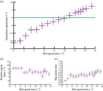
Typical features of the motion of a sphere on a vertical belt covered by a thin layer of viscous fluid are illustrated using the results shown in figure 2. These results are found over a wide range of sphere diameters, materials and film thicknesses, and they have been selected to illustrate generic features of the problem.

Figure 2. (a) The translation speed of a $12.7$
mm diameter polypropylene sphere on a
$12.7$
mm diameter polypropylene sphere on a $0.2$
mm layer plotted as a function of belt speed. (b) The rotation speed
$0.2$
mm layer plotted as a function of belt speed. (b) The rotation speed $\omega r$
of the sphere versus belt speed
$\omega r$
of the sphere versus belt speed $U$
. (c) The slip speed ratio as a function of belt speed. In this case, the slip speed ratio is defined as
$U$
. (c) The slip speed ratio as a function of belt speed. In this case, the slip speed ratio is defined as $ {\omega r}/{U_{\textit{net}}}$
, where
$ {\omega r}/{U_{\textit{net}}}$
, where $U_{\textit{net}}$
is the net speed of the sphere with respect to the belt.
$U_{\textit{net}}$
is the net speed of the sphere with respect to the belt.

Figure 3. A log–log plot of estimates for $ \textit{Re}$
at balance for viscous layers of various thicknesses:
$ \textit{Re}$
at balance for viscous layers of various thicknesses: $1.0$
,
$1.0$
, $0.75$
,
$0.75$
, $0.6$
,
$0.6$
, $0.5$
,
$0.5$
, $0.3$
,
$0.3$
, $0.2$
and
$0.2$
and $0.1$
mm. The lines are all linear least squares fits with gradients, respectively, of
$0.1$
mm. The lines are all linear least squares fits with gradients, respectively, of $2.54\pm 0.2$
,
$2.54\pm 0.2$
, $3.46 \pm 0.2$
,
$3.46 \pm 0.2$
, $3.47 \pm 0.3$
,
$3.47 \pm 0.3$
, $2.53 \pm 0.06$
,
$2.53 \pm 0.06$
, $2.93 \pm 0.09$
,
$2.93 \pm 0.09$
, $3.055 \pm 0.2$
and
$3.055 \pm 0.2$
and $1.55 \pm 0.2$
.
$1.55 \pm 0.2$
.
The graph in figure 2(a) is a chart of the translation speed of a $12.7$
mm diameter polypropylene sphere on a
$12.7$
mm diameter polypropylene sphere on a $0.2$
mm layer plotted as a function of the belt speed. In the notation used here, the upward motion of the belt is assigned to be in the positive direction. When the belt is stationary, the experiment is initiated by placing the sphere at the top of the belt and releasing it as described above. It rolls down the belt under gravity and capillary action causes it to adhere to the layer until it reaches the bottom of the belt. When the belt speed is set to specified increased values, the fall speed of the sphere decreases and the net translation speed from top to bottom also increases. The horizontal line in figure 2(a) represents an approximate balance where the belt speed matches the fall speed of the sphere, and hence it remains at a fixed position on the belt. It is observed that the time scales for the motion diverge as the balance speed is approached and the translation speed goes to zero as indicated in figure 2(a). The effects of small-scale fluctuations become evident at these slow speeds and this is a topic for further investigation. In principle, the location of the fixed position, where the fall speed matches the upward belt, could be anywhere along the belt. In practice, it is observed that there is a preferred location for the stationary point, which is
$0.2$
mm layer plotted as a function of the belt speed. In the notation used here, the upward motion of the belt is assigned to be in the positive direction. When the belt is stationary, the experiment is initiated by placing the sphere at the top of the belt and releasing it as described above. It rolls down the belt under gravity and capillary action causes it to adhere to the layer until it reaches the bottom of the belt. When the belt speed is set to specified increased values, the fall speed of the sphere decreases and the net translation speed from top to bottom also increases. The horizontal line in figure 2(a) represents an approximate balance where the belt speed matches the fall speed of the sphere, and hence it remains at a fixed position on the belt. It is observed that the time scales for the motion diverge as the balance speed is approached and the translation speed goes to zero as indicated in figure 2(a). The effects of small-scale fluctuations become evident at these slow speeds and this is a topic for further investigation. In principle, the location of the fixed position, where the fall speed matches the upward belt, could be anywhere along the belt. In practice, it is observed that there is a preferred location for the stationary point, which is ${\sim} 10$
mm below the axis of the upper pulley that holds the belt. Presumably, there is a slight thinning of the layer up the belt but we were unable to detect any clear change in the layer thickness. Typically, the sphere remains balanced at this location for days with no signs of movement up or down the belt.
${\sim} 10$
mm below the axis of the upper pulley that holds the belt. Presumably, there is a slight thinning of the layer up the belt but we were unable to detect any clear change in the layer thickness. Typically, the sphere remains balanced at this location for days with no signs of movement up or down the belt.
An increase in the belt speed above that required for balance causes the sphere to move up the belt. This part of the investigation is initiated by placing the sphere at the bottom of the belt. In this case, the sphere moves slowly to the top of the belt where it crosses over the top of it. There is a noticeable slowing of the translation motion as the balance speed is approached by adjusting the belt speed either upward or downward near the balance point. Again, time scales diverge near the balance speed and the motion is very slow, sometimes taking hours to settle. However, once the balance point has been reached, the location of the sphere remains fixed as long as the belt motion is maintained.
As described above, the sphere always rotates when on the viscous layer. The results shown in figure 2(b) illustrate the dependence of the rotation rate of the sphere on the belt speed. It can be seen that the rotation speed is essentially independent of the belt speed. This observation indicates that the sphere is fully supported by the fluid layer, and hence there is no net force on the sphere as the fluid is unable to support a shear stress. Gravity pulls the sphere downwards, and this is opposed by viscous shear at the surface of the sphere. The latter is a complicated interaction, since rotation of the sphere causes fluid to be carried over its surface. Hence, there are converging fluid layers located at the downstream area of the sphere and diverging layers at the upstream region.
Figure 2(c) is a graph of the slip speed ratio, which is defined here as the rotation speed of the sphere divided by its net translation speed $ {\omega r}/{U_{\textit{net}}}$
. Here
$ {\omega r}/{U_{\textit{net}}}$
. Here $U_{\textit{net}} =U_{\textit{Belt}}-U_{\textit{Trans}}$
, where
$U_{\textit{net}} =U_{\textit{Belt}}-U_{\textit{Trans}}$
, where $U_{\textit{net}}$
is the net translation speed of the sphere,
$U_{\textit{net}}$
is the net translation speed of the sphere, $U_{\textit{Belt}}$
is the speed of the belt and
$U_{\textit{Belt}}$
is the speed of the belt and $U_{\textit{Trans}}$
is the relative translation speed of the sphere with respect to the belt. It can be seen that the slip speed ratio is approximately independent of the belt speed so that
$U_{\textit{Trans}}$
is the relative translation speed of the sphere with respect to the belt. It can be seen that the slip speed ratio is approximately independent of the belt speed so that $U_{\textit{net}}$
is constant.
$U_{\textit{net}}$
is constant.
4.2. Balance speeds
Shown in figure 3 is a log–log plot of the estimates of $ \textit{Re}$
at which balance is achieved for polypropylene spheres on
$ \textit{Re}$
at which balance is achieved for polypropylene spheres on $0.1,\ 0.2,\ 0.3,\ 0.5,\ 0.6,\ 0.75$
and
$0.1,\ 0.2,\ 0.3,\ 0.5,\ 0.6,\ 0.75$
and $1.0$
mm thick viscous films. The ordinate has been made dimensionless by dividing the radius of the sphere by the respective depth of the layer. The linear least squares fitted lines to the data have slopes
$1.0$
mm thick viscous films. The ordinate has been made dimensionless by dividing the radius of the sphere by the respective depth of the layer. The linear least squares fitted lines to the data have slopes ${\sim} 3 \pm 10\,\%$
indicating that balance is approximately proportional to the weight of the sphere. A clear exception to this are the data for the thinnest layer of
${\sim} 3 \pm 10\,\%$
indicating that balance is approximately proportional to the weight of the sphere. A clear exception to this are the data for the thinnest layer of $0.1$
mm where the slope is
$0.1$
mm where the slope is ${\sim} {1}/{2}$
that of the thicker layers. Surface roughness effects may well be significant in this case with intermittent contact between the two surfaces reducing the slip. Further support for the cubic relationship between the balance speed and the radii of the spheres is provided by the results shown in figure 4, which is a plot of the empirically scaled value of
${\sim} {1}/{2}$
that of the thicker layers. Surface roughness effects may well be significant in this case with intermittent contact between the two surfaces reducing the slip. Further support for the cubic relationship between the balance speed and the radii of the spheres is provided by the results shown in figure 4, which is a plot of the empirically scaled value of $ \textit{Re}$
at balance versus
$ \textit{Re}$
at balance versus $ {r}/{h}$
. The same data are plotted here as in figure 3 but here the abscissa is empirically scaled by
$ {r}/{h}$
. The same data are plotted here as in figure 3 but here the abscissa is empirically scaled by $( {h_n}/{h_{0.1}})^3$
which produces a collapse of the data.
$( {h_n}/{h_{0.1}})^3$
which produces a collapse of the data.

Figure 4. Log–log plot for polypropylene spheres of the dependence of the scaled $ \textit{Re}$
for balance plotted as a function of sphere radius made dimensionless using the film thickness. Reynolds number
$ \textit{Re}$
for balance plotted as a function of sphere radius made dimensionless using the film thickness. Reynolds number $ \textit{Re}$
has been empirically scaled by the ratio
$ \textit{Re}$
has been empirically scaled by the ratio $({h_n}/{h_{0.1}})^3$
and
$({h_n}/{h_{0.1}})^3$
and $n$
denotes layers with thicknesses of
$n$
denotes layers with thicknesses of $0.1,\ 0.2,\ 0.3,\ 0.5$
and
$0.1,\ 0.2,\ 0.3,\ 0.5$
and $0.6$
mm. The linear least squares fitted line has slope of
$0.6$
mm. The linear least squares fitted line has slope of $2.27\pm 0.02$
.
$2.27\pm 0.02$
.
Evidence for the dependence of the balance speed on the mass of the sphere is further supported by the data presented in figure 5. Here, the estimates of $ \textit{Re}$
at balance for spheres of various materials have been scaled by the ratio of the density of the material with respect to
$ \textit{Re}$
at balance for spheres of various materials have been scaled by the ratio of the density of the material with respect to $\rho$
for steel,
$\rho$
for steel, $\delta ^*= {\rho _{\textit{steel}}}/{\rho _{\textit{mat}}}$
, where
$\delta ^*= {\rho _{\textit{steel}}}/{\rho _{\textit{mat}}}$
, where $\rho _{\textit{steel}}$
is
$\rho _{\textit{steel}}$
is $7800$
kg m
$7800$
kg m $^{-3}$
(the density of steel) and
$^{-3}$
(the density of steel) and $\rho _{\textit{mat}}$
is the density of the respective material. A highly satisfactory collapse of the data can be seen, and the slope of the least squares fitted line is
$\rho _{\textit{mat}}$
is the density of the respective material. A highly satisfactory collapse of the data can be seen, and the slope of the least squares fitted line is $ -2.89 \pm 0.08$
, which provides supporting evidence for the dependence of the balance speed on the weight of the sphere.
$ -2.89 \pm 0.08$
, which provides supporting evidence for the dependence of the balance speed on the weight of the sphere.

Figure 5. The balance speed for spheres with diameters in the range $6.0$
to
$6.0$
to $15.0$
mm and a range materials on a
$15.0$
mm and a range materials on a $0.3$
mm layer of silicone oil. The materials used are steel, glass, polypropylene, acetate and rubber as indicated in the key in the bottom right-hand corner. The
$0.3$
mm layer of silicone oil. The materials used are steel, glass, polypropylene, acetate and rubber as indicated in the key in the bottom right-hand corner. The $y$
axis has been scaled by the density ratio of the material with respect to
$y$
axis has been scaled by the density ratio of the material with respect to $\rho$
for steel,
$\rho$
for steel, $\delta ^*= {\rho _{\textit{steel}}}/{\rho _{\textit{mat}}}$
, where
$\delta ^*= {\rho _{\textit{steel}}}/{\rho _{\textit{mat}}}$
, where $\rho _{\textit{steel}}$
is
$\rho _{\textit{steel}}$
is $7800$
kg m
$7800$
kg m $^{-3}$
(the density of steel) and
$^{-3}$
(the density of steel) and $\rho _{\textit{mat}}$
is the density of the respective material. The least squares fitted line has a slope of
$\rho _{\textit{mat}}$
is the density of the respective material. The least squares fitted line has a slope of $-2.89 \pm 0.08$
.
$-2.89 \pm 0.08$
.
4.3. Slip speed ratio
As defined above, the slip speed ratio is $ {\omega r}/{U_{\textit{net}}}$
, where
$ {\omega r}/{U_{\textit{net}}}$
, where $U_{\textit{net}} =U_{\textit{Belt}}-U_{\textit{Trans}}$
. The feature of the belt problem that this takes into account is that the sphere typically translates with respect to the belt. Moreover, results such as those presented in figure 2(b) indicate that the rotation rate of the sphere is approximately independent of the belt speed. Hence, in order to simplify the analysis,
$U_{\textit{net}} =U_{\textit{Belt}}-U_{\textit{Trans}}$
. The feature of the belt problem that this takes into account is that the sphere typically translates with respect to the belt. Moreover, results such as those presented in figure 2(b) indicate that the rotation rate of the sphere is approximately independent of the belt speed. Hence, in order to simplify the analysis, $\omega$
is therefore primarily measured at balance, where
$\omega$
is therefore primarily measured at balance, where $U_{\textit{sph}}\approx 0$
, although the full relationship was checked at other belt speeds. Figure 6(a) is a plot of the rotation speed of steel spheres versus belt speed for a film with thickness of
$U_{\textit{sph}}\approx 0$
, although the full relationship was checked at other belt speeds. Figure 6(a) is a plot of the rotation speed of steel spheres versus belt speed for a film with thickness of $0.3$
mm. The spheres have radii in the range
$0.3$
mm. The spheres have radii in the range $3.0$
to
$3.0$
to $15.0$
mm. The least squares fitted line provides a good-quality fit to the data and indicates a slip speed ratio
$15.0$
mm. The least squares fitted line provides a good-quality fit to the data and indicates a slip speed ratio $ {\omega r}/{U} \approx 0.651 \pm 0.02$
. As is discussed below, this value of
$ {\omega r}/{U} \approx 0.651 \pm 0.02$
. As is discussed below, this value of ${\sim} {2}/{3}$
is typical for two-track states for both the belt and the cylinder.
${\sim} {2}/{3}$
is typical for two-track states for both the belt and the cylinder.

Figure 6. (a) The estimate at balance of $\omega r$
plotted versus
$\omega r$
plotted versus $U$
for steel spheres on the belt with a
$U$
for steel spheres on the belt with a $0.3$
mm thick film. The spheres have radii in the range
$0.3$
mm thick film. The spheres have radii in the range $3.0$
to
$3.0$
to $15.0$
mm in steps of
$15.0$
mm in steps of ${\sim} 0.5$
mm. The least squares fitted line has a slope of
${\sim} 0.5$
mm. The least squares fitted line has a slope of $0.651 \pm 0.02$
. (b) The estimate at balance of
$0.651 \pm 0.02$
. (b) The estimate at balance of $\omega r$
plotted versus belt speed for polypropylene spheres on a belt. The spheres have radii in the range
$\omega r$
plotted versus belt speed for polypropylene spheres on a belt. The spheres have radii in the range $3.0$
to
$3.0$
to $10.0$
mm in steps of
$10.0$
mm in steps of ${\sim} 0.5$
mm. Data recorded with film thicknesses of
${\sim} 0.5$
mm. Data recorded with film thicknesses of $0.1,\ 0.2,\ 0.3,\ 0.5,\ 0.6$
and
$0.1,\ 0.2,\ 0.3,\ 0.5,\ 0.6$
and $0.75$
mm. The fitted line has a slope of
$0.75$
mm. The fitted line has a slope of $0.677 \pm 0.04$
. Small effects of surface roughness are visible in the data points for the
$0.677 \pm 0.04$
. Small effects of surface roughness are visible in the data points for the $ 0.1$
mm film, represented by (+) symbols.
$ 0.1$
mm film, represented by (+) symbols.
In figure 6(b) we show results for the relationship between belt speed and the rotation speed for polypropylene spheres with radii in the range $3$
to
$3$
to $15$
mm with film thicknesses of
$15$
mm with film thicknesses of $0.1,\ 0.2,\ 0.3,\ 0.5,\ 0.6$
and
$0.1,\ 0.2,\ 0.3,\ 0.5,\ 0.6$
and $0.75$
mm. The least squares fitted line in this case indicates a slip speed ratio
$0.75$
mm. The least squares fitted line in this case indicates a slip speed ratio $ {\omega r}/{U} \approx 0.677 \pm 0.04$
. It can be seen that the results are essentially independent of film thickness, although there is some evidence for the effects of surface roughness as the results for the
$ {\omega r}/{U} \approx 0.677 \pm 0.04$
. It can be seen that the results are essentially independent of film thickness, although there is some evidence for the effects of surface roughness as the results for the $0.1$
mm film shown by (+) symbols are slightly above all other points.
$0.1$
mm film shown by (+) symbols are slightly above all other points.
Finally, we show in figure 7 experimental results which help confirm that the torque balance is generated between viscous shear between the film and the sphere. Thus, the rotation rate of the sphere scales as ${\approx} r^2$
which is consistent with
${\approx} r^2$
which is consistent with $U \propto r^3$
and hence
$U \propto r^3$
and hence $\omega = U/r \propto r^2$
. There is clear evidence for the effects of surface roughness in the results obtained for the thinnest layer,
$\omega = U/r \propto r^2$
. There is clear evidence for the effects of surface roughness in the results obtained for the thinnest layer, $0.1$
mm, and the observed values of
$0.1$
mm, and the observed values of $\omega$
are a factor of
$\omega$
are a factor of ${\sim} 2$
above those found for thicker layers. Clearly, there are complex fluid interactions at the converging and diverging surface regions; however, these appear to be secondary effects, and the primary driving mechanism is the torque balance.
${\sim} 2$
above those found for thicker layers. Clearly, there are complex fluid interactions at the converging and diverging surface regions; however, these appear to be secondary effects, and the primary driving mechanism is the torque balance.

Figure 7. Log–log plot of the rotation frequency of polypropylene spheres as a function of the radius of the sphere. The best-fit line to the majority of the data is shown and has a slope of $2.26 \pm 0.25$
. The effects of roughness can be seen in the data for the
$2.26 \pm 0.25$
. The effects of roughness can be seen in the data for the $0.1$
mm film. In this case the rotation frequencies are a factor of
$0.1$
mm film. In this case the rotation frequencies are a factor of ${\approx} 2$
greater than those found with thicker layers. These data are not included in the least squares fit.
${\approx} 2$
greater than those found with thicker layers. These data are not included in the least squares fit.
4.3.1. Principal results obtained with the vertical belt
The main finding is that almost all the motion of a sphere levitated on a thin viscous film on a moving vertical belt is transient. The exception to this occurs at a particular belt speed when there is balance between gravity and viscous action. In this case, the sphere sits at a single location over very long periods of time. The balance speed is proportional to the mass of the sphere as shown by its proportionality to $r^3$
and the density
$r^3$
and the density $\rho$
.
$\rho$
.
Capillary forces cause the sphere to adhere to the film which wraps around the sphere as it rotates. There is a circle of intersection between the sphere and the layer and two tracks are left in the layer upstream of the sphere. The rotation rate of the sphere is independent of the belt speed and it is linearly proportional to its radius. Finally, the rotation rate is independent of the film thickness.
5. The horizontal cylinder
The rotating-cylinder experiments are performed in the same temperature-controlled laboratory as those using the belt. The apparatus comprises a precision-ground glass cylinder with an inner diameter of $130 \pm 0.05$
mm and a wall thickness of
$130 \pm 0.05$
mm and a wall thickness of $5$
mm, which is centrally mounted in a precision bearing. A schematic end-view diagram showing the essential features of the apparatus is given in figure 8. The cylinder is
$5$
mm, which is centrally mounted in a precision bearing. A schematic end-view diagram showing the essential features of the apparatus is given in figure 8. The cylinder is $120$
mm long and has an aluminium ring
$120$
mm long and has an aluminium ring $1$
cm wide attached at one end using O-ring seals. The cylinder is held horizontally using a precision bearing at one end, which is mounted in a housing weighing
$1$
cm wide attached at one end using O-ring seals. The cylinder is held horizontally using a precision bearing at one end, which is mounted in a housing weighing $5$
kg. The apparatus is levelled using three adjustable feet on a machined aluminium plate to make fine adjustments of the level. The levelling was checked using an engineer’s level.
$5$
kg. The apparatus is levelled using three adjustable feet on a machined aluminium plate to make fine adjustments of the level. The levelling was checked using an engineer’s level.

Figure 8. A schematic diagram of the cylinder apparatus. An end view is given to show the mounting of the scraper.
At the start of each experiment, an ${\sim} 7.5$
mm deep puddle of viscous silicone fluid is placed in the bottom of the cylinder. The cylinder is rotated slowly, and the fluid is dragged through the gap between the wall of the moving cylinder and a long machined knife edge, which is held by a
${\sim} 7.5$
mm deep puddle of viscous silicone fluid is placed in the bottom of the cylinder. The cylinder is rotated slowly, and the fluid is dragged through the gap between the wall of the moving cylinder and a long machined knife edge, which is held by a $1$
cm steel rod mounted on the axis. A layer of fluid is formed along the length of the cylinder and dragged around the surface of the rotating cylinder. The gap between the knife edge and the cylinder wall is set using engineer’s feeler gauges. The knife-edge scraper is found to produce uniform viscous films of prescribed thicknesses. A schematic diagram of an end-on view of the experiment is given in figure 8.
$1$
cm steel rod mounted on the axis. A layer of fluid is formed along the length of the cylinder and dragged around the surface of the rotating cylinder. The gap between the knife edge and the cylinder wall is set using engineer’s feeler gauges. The knife-edge scraper is found to produce uniform viscous films of prescribed thicknesses. A schematic diagram of an end-on view of the experiment is given in figure 8.

Figure 9. (a,b) Examples of the steady states involved in levitating spheres on a viscous layer formed on the inside of a horizontal rotating cylinder. In these examples the steel spheres are both $16.0$
mm in diameter, the layer is
$16.0$
mm in diameter, the layer is $0.3$
mm thick and
$0.3$
mm thick and $ \textit{Re} = 0.0002$
in both images.
$ \textit{Re} = 0.0002$
in both images.
The cylinder is driven around using a feedback-controlled DC motor, which is attached to a pulley on the bearing via a toothed belt and either a 6 : 1, 50 : 1, or 100 : 1 gearbox, depending on the weight of the spheres. The speed of rotation was monitored using a calibrated optical shaft encoder, which produces $400$
pulses per revolution of the shaft. A Nikon
$400$
pulses per revolution of the shaft. A Nikon $400$
S camera mounted on a tripod is used to take photographs of the spheres, which were recorded on a laptop using the software suite DigiCam. Processing of the images is carried out using ImageJ, which enables the measurement of the position and rotation speed of the spheres. The majority of the experiments are performed using precision steel spheres; however, glass, rubber and various plastic spheres were also used, as detailed below.
$400$
S camera mounted on a tripod is used to take photographs of the spheres, which were recorded on a laptop using the software suite DigiCam. Processing of the images is carried out using ImageJ, which enables the measurement of the position and rotation speed of the spheres. The majority of the experiments are performed using precision steel spheres; however, glass, rubber and various plastic spheres were also used, as detailed below.
5.1. Principal features of rotating-cylinder experiments
The two important qualitative differences between the belt and cylinder experiments are that, firstly, the sphere always sits at a fixed location on the lower rising quadrant of the wall of the cylinder when the cylinder rotates at a set speed. Secondly, whereas a unique two-track state is observed downstream of the sphere on a belt, both single- and two-track steady states are found for the cylinder. The single-track state is observed when the sphere is located approximately on the mid-plane of the cylinder. The particular state which is observed depends on its history of creation, and images of both states are given in figure 9.

Figure 10. Plot of the angular position of a $19$
mm diameter steel sphere as a function of
$19$
mm diameter steel sphere as a function of $ \textit{Re}$
on a
$ \textit{Re}$
on a $0.3$
mm deep layer. The point labelled A corresponds to
$0.3$
mm deep layer. The point labelled A corresponds to ${\sim} 0^\circ$
at the bottom of the cylinder and B is halfway up the side of the cylinder at
${\sim} 0^\circ$
at the bottom of the cylinder and B is halfway up the side of the cylinder at ${\sim} 90^\circ$
. The sphere transitions to the single-track state when
${\sim} 90^\circ$
. The sphere transitions to the single-track state when $ \textit{Re}$
is increased above the value at B. It remains in the single-track state at
$ \textit{Re}$
is increased above the value at B. It remains in the single-track state at ${\approx} 90^\circ$
along the path labelled BCD and the motion of the sphere is time-dependent between B and C. The motion becomes steady at C and further reduction in
${\approx} 90^\circ$
along the path labelled BCD and the motion of the sphere is time-dependent between B and C. The motion becomes steady at C and further reduction in $ \textit{Re}$
below the value corresponding to D causes the sphere to transition back to the two-track state along AB.
$ \textit{Re}$
below the value corresponding to D causes the sphere to transition back to the two-track state along AB.
Hence, the dynamical equivalence between the experiments with the belt and the cylinder is not complete. In the results shown in figure 10, each symbol along ABCD designates a fixed point of the motion of the sphere on the viscous layer which coats the inner wall of the rotating cylinder. Hence, the sphere sits at a particular location on the layer on the upward-moving wall of the cylinder, as indicated in figure 10. The location of each fixed point is determined by the rotation speed of the cylinder, and the sphere remains at this particular location as long as the cylinder is rotated at a given speed. Moreover, if the sphere is displaced from the location, it will return to the fixed point after a short transient. Thus, in the rotating-cylinder experiment, the sphere is always at a fixed point.
As indicated by the locus AB in figure 10, the two-track fixed-point state is located at increasing angular locations as the cylinder speed is increased. The mid-plane is reached close to the point labelled B. Further increase in the speed of the cylinder gives rise to a transition to a single-track state. This state can be oscillatory where the sphere moves up and down with an amplitude of motion of ${\sim} 5$
mm for larger-diameter spheres. However, the transition is between steady states when
${\sim} 5$
mm for larger-diameter spheres. However, the transition is between steady states when $r \leqq 7$
mm.
$r \leqq 7$
mm.
When the rotation speed of the cylinder is reduced in the case shown in figure 10, the amplitude of the oscillatory motion decreases until a steady state is observed at the point labelled C. The sphere now sits on the mid-plane of the cylinder in a single-track state as in figure 9(b). Further reduction in the rotation speed of the cylinder leads to a transition back to the two-track state when a speed corresponding to the point labelled D is reached. The transition is catastrophic, with the sphere usually falling a few centimetres down the wall. Hence, the creation and loss of the single-track state involves significant hysteresis in the control parameter, the speed of rotation of the cylinder.
5.1.1. Transitions between single- and two-track states
Loci of the transition points between single- and two-track states for a range of steel sphere diameters are shown in figure 11. The experiment is initiated by placing the sphere in the cylinder, which is rotating at a very slow rate. Hence, the sphere initially sits rotating on the layer close to the bottom of the cylinder. As the speed of rotation of the cylinder is increased to new set values, the sphere rises to new fixed positions up the rising wall as discussed above. The sphere continues to rotate leaving two ridges in the layer above it as shown in figure 9(a) or inset (b) in figure 11. When $ \textit{Re}$
is increased so that the line labelled AB in figure 11 is crossed, a sudden transition to an oscillatory single-track state (figure 9
b) is observed. Subsequent reduction of the rotation rate of the cylinder leads to a steady single-track state with the sphere located close to the mid-plane of the cylinder. Further reduction in the cylinder speed leads to a catastrophic transition back to a two-track state when the path labelled CD in figure 11 is crossed.
$ \textit{Re}$
is increased so that the line labelled AB in figure 11 is crossed, a sudden transition to an oscillatory single-track state (figure 9
b) is observed. Subsequent reduction of the rotation rate of the cylinder leads to a steady single-track state with the sphere located close to the mid-plane of the cylinder. Further reduction in the cylinder speed leads to a catastrophic transition back to a two-track state when the path labelled CD in figure 11 is crossed.

Figure 11. Loci of estimates of limit points for the transition between single- and double-track states plotted on a log–log scale. The layer is $0.4$
mm deep and the spheres are steel as in the inset images. The least squares fitted lines have slopes of
$0.4$
mm deep and the spheres are steel as in the inset images. The least squares fitted lines have slopes of $\text{AB} =1.96$
and
$\text{AB} =1.96$
and $\text{CD} = 1.56$
. The two-track state shown in inset (b) exists for all sphere radii at values of
$\text{CD} = 1.56$
. The two-track state shown in inset (b) exists for all sphere radii at values of $ \textit{Re}$
below AB. A transition to the one-track state occurs when AB is crossed by increasing
$ \textit{Re}$
below AB. A transition to the one-track state occurs when AB is crossed by increasing $ \textit{Re}$
as indicated by the arrowed path. The transition involves time-dependent motion for large-diameter spheres corresponding to points near B. The transition involves steady states otherwise. The reverse transition occurs when CD is crossed as indicated by the second downward-pointing arrow. This transition is observed to be between steady states. Hence, there is hysteresis between the two transitions.
$ \textit{Re}$
as indicated by the arrowed path. The transition involves time-dependent motion for large-diameter spheres corresponding to points near B. The transition involves steady states otherwise. The reverse transition occurs when CD is crossed as indicated by the second downward-pointing arrow. This transition is observed to be between steady states. Hence, there is hysteresis between the two transitions.

Figure 12. Loci of critical points for transition between single- and double-track states. Steel spheres with diameters ranging from $5$
to
$5$
to $19$
mm in
$19$
mm in $1$
mm steps. The film thicknesses are
$1$
mm steps. The film thicknesses are $0.1\,(\rm green), 0.2\,(blue), 0.3\,(brown), 0.4\,(yellow)$
and
$0.1\,(\rm green), 0.2\,(blue), 0.3\,(brown), 0.4\,(yellow)$
and $0.5$
(dark blue) mm. The stated colours have been used to mark the data points for a particular film thickness.
$0.5$
(dark blue) mm. The stated colours have been used to mark the data points for a particular film thickness.
The locus of the transition between two-track and single-track states is labelled AB in figure 11 and that for the reverse transition CD. There is significant hysteresis involved in these transitions so that the steady-solution surface contains a pair of folds which perhaps approach each other as $r$
is decreased. The path AB has a slope of
$r$
is decreased. The path AB has a slope of ${\approx} 2$
which is consistent with proportionality to the surface area of the sphere. The lower locus CD has a slope of
${\approx} 2$
which is consistent with proportionality to the surface area of the sphere. The lower locus CD has a slope of ${\sim} 1.6$
which is also consistent with the importance of the surface area of the sphere on the transition from the one- to two-track state. These results are in marked contrast to the dependence on the volume for the balance speed found in the results for the belt.
${\sim} 1.6$
which is also consistent with the importance of the surface area of the sphere on the transition from the one- to two-track state. These results are in marked contrast to the dependence on the volume for the balance speed found in the results for the belt.
The effect of layer depth on the transitions between single- and two-track states is explored and the results for steel spheres are presented in figure 12. The results are plotted in the dimensionless form of $ \textit{Re}$
versus sphere radius divided by layer thickness. It is clear that there is significant hysteresis present for all layer depths, which range from
$ \textit{Re}$
versus sphere radius divided by layer thickness. It is clear that there is significant hysteresis present for all layer depths, which range from $0.1$
to
$0.1$
to $0.5$
mm. The dependence on
$0.5$
mm. The dependence on $r$
steepens as the layer thickens and the gap between the loci narrows so that the paths of critical points almost overlap for the thicker layers.
$r$
steepens as the layer thickens and the gap between the loci narrows so that the paths of critical points almost overlap for the thicker layers.

Figure 13. Log–log plot of loci of critical points for transition between (AB) double- and single-track states and (CD) single to double track. The data are from experiments with polypropylene spheres and a film thickness of $0.4$
mm. The solid lines are linear least squares fits with slopes
$0.4$
mm. The solid lines are linear least squares fits with slopes $ \text{AB} \approx 2.5$
and
$ \text{AB} \approx 2.5$
and $ \text{CD}\approx 2.0$
. The inset images illustrate the states involved and a
$ \text{CD}\approx 2.0$
. The inset images illustrate the states involved and a $25$
mm diameter sphere is used in this case.
$25$
mm diameter sphere is used in this case.
It was shown in the results given in figure 5 that the dependence of the balance speed on sphere radius $r$
scales with the density of the sphere. Hence, the mass of the sphere is key in the force balance. The results discussed thus far for the cylinder experiment have all been for steel spheres. To establish the role of the sphere’s density in these results, we show in figure 13 the response diagram for the single- and double-track states of light polypropylene spheres. It can be seen immediately that the same qualitative features are present in a hysteretic transition between single- and two-track states.
$r$
scales with the density of the sphere. Hence, the mass of the sphere is key in the force balance. The results discussed thus far for the cylinder experiment have all been for steel spheres. To establish the role of the sphere’s density in these results, we show in figure 13 the response diagram for the single- and double-track states of light polypropylene spheres. It can be seen immediately that the same qualitative features are present in a hysteretic transition between single- and two-track states.
6. Slip speed ratio for spheres on inner wall of cylinder
The spheres rotate when sitting at their respective fixed positions on the viscous layer on the inside of the cylinder. As in the belt experiment, the surface speed of the sphere is less than that of the wall. Hence, a defined slip speed ratio $ {U}/{\omega r} \lt 1.0$
exists since there is a lubrication layer between the two surfaces. Visual evidence for the positioning of the lubrication layer can be seen in the images shown in figure 9 where the approximately circular intersection between the sphere and the viscous film is apparent. There is a pronounced non-circular intersection in the two-track state as in figure 9(a), whereas the partly circular region is virtually complete for the one-track state in figure 9(b). The results for the dependence of the slip speed on cylinder speed are first discussed for the two-track state. This state exists over a wide range of cylinder speeds, and a significant feature is that two tracks are left behind the sphere in the fluid layer as in figure 9(a). The two-track state exists over the range of cylinder rotation rates from low speeds, where the sphere is located near the bottom of the cylinder, to higher speeds, where the sphere sits just below the mid-plane.
$ {U}/{\omega r} \lt 1.0$
exists since there is a lubrication layer between the two surfaces. Visual evidence for the positioning of the lubrication layer can be seen in the images shown in figure 9 where the approximately circular intersection between the sphere and the viscous film is apparent. There is a pronounced non-circular intersection in the two-track state as in figure 9(a), whereas the partly circular region is virtually complete for the one-track state in figure 9(b). The results for the dependence of the slip speed on cylinder speed are first discussed for the two-track state. This state exists over a wide range of cylinder speeds, and a significant feature is that two tracks are left behind the sphere in the fluid layer as in figure 9(a). The two-track state exists over the range of cylinder rotation rates from low speeds, where the sphere is located near the bottom of the cylinder, to higher speeds, where the sphere sits just below the mid-plane.
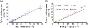
Shown in figure 14 is a graph of the rotation rate of the sphere $\omega r$
plotted as a function of the rotation rate of the cylinder
$\omega r$
plotted as a function of the rotation rate of the cylinder $U$
. The data are for a range of polypropylene spheres with diameters between
$U$
. The data are for a range of polypropylene spheres with diameters between $6$
and
$6$
and $30$
mm and steel spheres with diameters ranging from
$30$
mm and steel spheres with diameters ranging from $6$
to
$6$
to $25$
mm with viscous layer depths between
$25$
mm with viscous layer depths between $0.2$
and
$0.2$
and $0.5$
mm in steps of
$0.5$
mm in steps of $0.1$
mm.
$0.1$
mm.
It is clear from these results that the rotation rate of the sphere does not depend on the layer depth and there appears to be a linear dependence of the ratio of the surface speeds of the sphere and the wall. In fact, an empirical least squares fit of a straight line to all of the data, which has an error of ${\approx} 0.5\,\%$
, has a slope of
${\approx} 0.5\,\%$
, has a slope of ${\sim} 0.649$
indicating that the slip speed ratio is a constant with a value of
${\sim} 0.649$
indicating that the slip speed ratio is a constant with a value of ${\sim} {2}/{3}$
which is close to the result for the belt data discussed above.
${\sim} {2}/{3}$
which is close to the result for the belt data discussed above.

Figure 14. Plot of $\omega r$
versus
$\omega r$
versus $U$
for two-track state for all film thicknesses and all steel and polypropylene sphere diameters. Data for steel spheres are marked by pluses and those for polypropylene spheres by crosses. Error bars are indicated on the vertical lines in the data markers. The least squares fitted line has a gradient of
$U$
for two-track state for all film thicknesses and all steel and polypropylene sphere diameters. Data for steel spheres are marked by pluses and those for polypropylene spheres by crosses. Error bars are indicated on the vertical lines in the data markers. The least squares fitted line has a gradient of $0.649$
with a fit error of
$0.649$
with a fit error of ${\sim} 0.5\,\%$
. Hence, the slip speed ratio for all spheres and all film thicknesses is
${\sim} 0.5\,\%$
. Hence, the slip speed ratio for all spheres and all film thicknesses is ${\approx} {2}/{3}$
.
${\approx} {2}/{3}$
.

Figure 15. Plot of the slip speed ratio ${\omega r}/{U}$
for single-track states with polypropylene spheres on a film thickness of
${\omega r}/{U}$
for single-track states with polypropylene spheres on a film thickness of $0.4$
mm. The experimental data points are for spheres with radii of
$0.4$
mm. The experimental data points are for spheres with radii of $6.3,\ 7.9$
and
$6.3,\ 7.9$
and $9.5$
mm. The solid lines are calculated using the model given in Ockendon et al. (Reference Ockendon, Ockendon and Mullin2024). The solid lines correspond to
$9.5$
mm. The solid lines are calculated using the model given in Ockendon et al. (Reference Ockendon, Ockendon and Mullin2024). The solid lines correspond to $9.5$
mm (lower),
$9.5$
mm (lower), $7.9$
mm (middle) and
$7.9$
mm (middle) and $6.3$
mm (upper). The error bars on the experimental data are typically
$6.3$
mm (upper). The error bars on the experimental data are typically ${\approx} 5 \,\%$
.
${\approx} 5 \,\%$
.
An analysis of the results for the single-track states proceeds using the predictions of the model reported in Ockendon et al. (Reference Ockendon, Ockendon and Mullin2024). The experimental results for this case are presented in figure 15 for polypropylene spheres on a $ 0.4$
mm layer, shown in quantitative comparison with the predictions from theory, which are the respective solid lines. Here, the sphere is located at
$ 0.4$
mm layer, shown in quantitative comparison with the predictions from theory, which are the respective solid lines. Here, the sphere is located at $90^\circ$
for all observations of the single-track state.
$90^\circ$
for all observations of the single-track state.
The accord between theory and experiment is very satisfactory. As predicted by theory, and unlike the experimental results for the two-track state discussed above, the slip speed ratio is not precisely constant and it also depends on the weight of the sphere $m$
.
$m$
.
Presented in figure 16 are results of an investigation into the slip speed ratio for steel spheres levitated in the single-track state on fluid layers ranging in depth from $0.2$
to
$0.2$
to $0.5$
mm. Overall, good general accord is found between theory and experiment since the experimental results are bounded by the dependencies predicted by the theory of Ockendon et al. (Reference Ockendon, Ockendon and Mullin2024). However, the detailed dependence on sphere size discussed above in connection with the results for lighter polypropylene spheres presented in figure 15 is not evident with the steel spheres. Instead, the experimental results appear to be proportional to the cylinder speed and an empirical linear least squares fit of a line with a slope of
$0.5$
mm. Overall, good general accord is found between theory and experiment since the experimental results are bounded by the dependencies predicted by the theory of Ockendon et al. (Reference Ockendon, Ockendon and Mullin2024). However, the detailed dependence on sphere size discussed above in connection with the results for lighter polypropylene spheres presented in figure 15 is not evident with the steel spheres. Instead, the experimental results appear to be proportional to the cylinder speed and an empirical linear least squares fit of a line with a slope of $ 0.549\pm 0.003$
provides an excellent match to the data. Hence, the slip speed ratio is approximately constant at
$ 0.549\pm 0.003$
provides an excellent match to the data. Hence, the slip speed ratio is approximately constant at ${\approx} {1}/{2}$
, and hence there is a greater slip than with the two-track state.
${\approx} {1}/{2}$
, and hence there is a greater slip than with the two-track state.

Figure 16. Comparison between theory and experiment for the slip speed dependence of the single-track state using steel spheres. Plot of $\omega r$
versus
$\omega r$
versus $U$
where sphere diameters of
$U$
where sphere diameters of $12$
mm (upper yellow line) and
$12$
mm (upper yellow line) and $19$
mm (lower red line) have been used in calculations using the theory of Ockendon et al. (Reference Ockendon, Ockendon and Mullin2024). The experimental data are for steel spheres with diameters ranging from
$19$
mm (lower red line) have been used in calculations using the theory of Ockendon et al. (Reference Ockendon, Ockendon and Mullin2024). The experimental data are for steel spheres with diameters ranging from $8$
to
$8$
to $19$
mm. The film thicknesses are
$19$
mm. The film thicknesses are $0.1,\ 0.2,\ 0.3$
and
$0.1,\ 0.2,\ 0.3$
and $0.5$
mm. The least squares fitted line (thick green/blue line) has a gradient of
$0.5$
mm. The least squares fitted line (thick green/blue line) has a gradient of $0.545\pm 0.003$
.
$0.545\pm 0.003$
.
6.1. Principal results obtained with the horizontal rotating cylinder
The central feature of the results obtained with the rotating cylinder is that the sphere always sits at a set of fixed spatial locations. They exist in the bottom quadrant of the cylinder on the side where the wall rises. There are two distinct stationary states. In one, the sphere leaves two tracks in the film, whereas in the other, a single track is formed. There is a hysteretic transition between the states. Hence, there exists a range of $ \textit{Re}$
where both states coexist. The loci of the critical points for transition is
$ \textit{Re}$
where both states coexist. The loci of the critical points for transition is $\propto r^2$
which suggests the surface area of the sphere is important. The slip speed ratio is in agreement with theory for the single-track state. However, an empirical scaling of this quantity produces a ratio of
$\propto r^2$
which suggests the surface area of the sphere is important. The slip speed ratio is in agreement with theory for the single-track state. However, an empirical scaling of this quantity produces a ratio of $ {1}/{2}$
. On the other hand, the slip speed ratio for the two-track state is
$ {1}/{2}$
. On the other hand, the slip speed ratio for the two-track state is $ {2}/{3}$
, which is in accord with the results found for the belt.
$ {2}/{3}$
, which is in accord with the results found for the belt.
7. Conclusions
Experimental results for investigations of the levitation of spheres on viscous layers have been presented. The experiments were performed using a planar moving vertically oriented wall. The second configuration was a curved wall with a thin viscous layer on the inside of a horizontal rotating cylinder.
A significant qualitative difference between the two configurations is that levitation of the sphere on the plane wall is a transient with the exception of the special case where the speed of the wall matches the fall speed of the sphere. Hence the sphere generally travels with respect to the wall but long-term balance at a particular location is achieved under the special conditions of matching speeds.
This is qualitatively different from the case where the sphere is levitated on a film on the inside of a rotating horizontal cylinder. In this case, levitation occurs at a series of fixed locations below the mid-plane of the rising wall of the cylinder, i.e. the sphere does not move with respect to the cylinder when it is rotated at a fixed speed.
A common feature in both cases is that the circle of intersection between the sphere and the viscous film gives rise to two tracks or ridges in the fluid which pass over the sphere and move up the wall with the layer. In this configuration the sphere rotates with respect to the moving wall with a slip speed ratio of ${\approx} {2}/{3}$
which is independent of sphere size and layer depth. The reason for this robust simple ratio is not understood at present and it is in marked contrast to the well-established ratio of
${\approx} {2}/{3}$
which is independent of sphere size and layer depth. The reason for this robust simple ratio is not understood at present and it is in marked contrast to the well-established ratio of ${\approx} {1}/{4}$
(Goldman, Cox & Brenner Reference Goldman, Cox and Brenner1967; Ashmore, del Pino & Mullin Reference Ashmore, del Pino and Mullin2005) for a fully submerged sphere adjacent to a wall.
${\approx} {1}/{4}$
(Goldman, Cox & Brenner Reference Goldman, Cox and Brenner1967; Ashmore, del Pino & Mullin Reference Ashmore, del Pino and Mullin2005) for a fully submerged sphere adjacent to a wall.
As previously reported in Ockendon et al. (Reference Ockendon, Ockendon and Mullin2024), a second state with a single track is found over a range of speeds when the sphere is levitated on the mid-plane of the cylinder. Excellent accord both in overall structure and in detail is found between predictions of the derived lubrication model and the observations reported here. Specifically, the detailed dependence of the slip speed ratio on sphere size is apparent for light spheres but it is difficult to uncover these details with heavy spheres. Instead, in the latter case, a slip speed ratio of ${\sim} {1}/{2}$
emerges. The ratio is found to be independent of sphere size and film thickness. The success of the model of the single-track state is encouraging but the systematic behaviour of the more general two-track state remains a theoretical challenge.
${\sim} {1}/{2}$
emerges. The ratio is found to be independent of sphere size and film thickness. The success of the model of the single-track state is encouraging but the systematic behaviour of the more general two-track state remains a theoretical challenge.
Acknowledgements
The author is grateful to J. Chapman, A. Datta, M. Gueribi, L. Vanquin and S. Choudhry who carried out preliminary experiments on these systems. He is also grateful to D. Vella for the laboratory space in the Observatory in the Mathematical Institute and K. Long for help with the cylinder experiment. Finally, he is very grateful to H. Ockendon and J. Ockendon for continuing support and interest in this work. Their insights have led to significant progress with this research. They also improved an earlier version of this paper and helped with Appendix A.
Declaration of interests
The author reports no conflict of interest.
Appendix A. The lubrication model for a single-track state
In Ockendon et al. (Reference Ockendon, Ockendon and Mullin2024) it is shown that a circular lubrication layer can exist between the sphere and the cylinder in the single-track state. Using polar coordinates $\hat {r},\theta$
based at the centre of the circle, the pressure
$\hat {r},\theta$
based at the centre of the circle, the pressure $p$
in the layer takes the form
$p$
in the layer takes the form
 \begin{align} p=\rho _{\textit{fluid}}\nu \sqrt {\frac {r}{h^3}}(U+\omega r)\hat {F}(\hat {r}) \cos\theta . \end{align}
Then the lubrication equations imply that $\hat {F}$
satisfies
$\hat {F}$
satisfies
 \begin{align} \hat {r}^2\left(1+\frac {\hat {r}^2}{2}\right)\frac {{\rm d}^2{\hat {F}}}{{\rm d} \hat {r}^2} + \hat {r}\left(1+\frac {7}{2}\hat {r}^2\right)\frac {{\rm d}{\hat {F}}}{{\rm d} \hat {r}}- \left(1 + \frac {\hat {r}^2}{2}\right){\hat {F}} = \frac {6\hat {r}^3}{\left(1+\frac {\hat {r}^2}{2}\right)^2}, \end{align}
with $\hat {F}(0)=0$
and
$\hat {F}(0)=0$
and $\hat {F}(\lambda )=0$
, where
$\hat {F}(\lambda )=0$
, where $\lambda$
is a parameter to be determined. The two equations for the equilibrium of the sphere are now sufficient to determine
$\lambda$
is a parameter to be determined. The two equations for the equilibrium of the sphere are now sufficient to determine $\lambda$
and
$\lambda$
and $\omega$
and can be reduced to
$\omega$
and can be reduced to
 \begin{align} \frac {\omega r}{U} = \frac {4\log \big(1+\frac {1}{2}{\lambda }^2\big) - I(\lambda )}{4\log \big(1+\frac {1}{2}{\lambda }^2\big) + I(\lambda )} \quad \text{and} \quad \frac {2\pi \rho _{\textit{fluid}} \nu r U}{mg} = \frac {1}{4\log \big(1+\frac {1}{2}{\lambda }^2\big)} + \frac {1}{I(\lambda )}, \end{align}
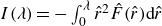
where $I(\lambda )= -\int _{0}^{\lambda } \hat {r}^2 \hat {F}(\hat {r}) {\rm d}\hat {r}$
. Eliminating
$I(\lambda )= -\int _{0}^{\lambda } \hat {r}^2 \hat {F}(\hat {r}) {\rm d}\hat {r}$
. Eliminating $\lambda$
between these two expressions allows us to plot
$\lambda$
between these two expressions allows us to plot ${\omega r}/{U}$
as a function of
${\omega r}/{U}$
as a function of $U$
in figure 15 and
$U$
in figure 15 and $\omega r$
against
$\omega r$
against $U$
in figure 16.
$U$
in figure 16.


 Open access