


1. Introduction
As technology advances, the semiconductor and aerospace industries increasingly require an understanding of flow physics at rarefied conditions. In semiconductor fabrication environments, many processes, including the use of free-jets, occur under vacuum conditions to enhance deposition efficiency, plasma generation and purity. Historically, the understanding of fluid flow in vacuum conditions focused mainly on the overall gas concentration within the processing equipment, allowing operation without a detailed understanding of the flow structure. However, as these processes have become more sophisticated and miniaturised, achieving desired yields without a thorough understanding of the flow dynamics has become increasingly difficult. Consequently, there is a growing demand for insights into the flow physics that governs semiconductor fabrication processes, but the challenges of measuring flows under rarefied conditions often make this difficult to achieve. Research exists for the internal flows within semiconductor manufacturing facilities, such as chemical vapour deposition (CVD) systems, but since experimental investigations are challenging, most studies have relied on continuum computational fluid dynamics (CFD) simulations (Hash et al. Reference Hash, Mihopoulos, Govindan and Meyyappan2000; Setyawan et al. Reference Setyawan, Shimada, Ohtsuka and Okuyama2002; Li et al. Reference Li, Cai, Wu, Wang, Pei and Wang2019). The absence of experimental results raises concerns regarding the validity of the CFD. Issues such as wafer defects caused by nano-particles, which differ significantly from those in atmospheric pressure conditions, are also prominent in rarefied environments (Loth et al. Reference Loth, Tyler Daspit, Jeong, Nagata and Nonomura2021; Capecelatro & Wagner Reference Capecelatro and Wagner2024).
In outer space environments, spacecraft including satellites typically employ small rocket engines (thrusters) to eject high-temperature or high-pressure exhaust gases (plumes) at supersonic speeds through nozzles, to facilitate precise attitude and orbit control. In the vacuum of space, the internal flow within rocket nozzles transitions from a continuum to a rarefied flow regime (Sukesan & Shine Reference Sukesan and Shine2023). Consequently, the exhaust gas particles disperse not only downstream of the rocket nozzle, but also in many other directions and in a non-equilibrium state. In such instances, backflow of exhaust gases towards the spacecraft can result in disturbance forces/torques and thermal loads, in addition to causing contamination as the cold surfaces of the spacecraft adsorb these particles (Dettleff & Grabe Reference Dettleff and Grabe2011). Aside from thrusters, there are issues related to plume and surface interactions during spacecraft landings on planetary bodies, which differ from interactions that occur in Earth atmospheric conditions (Plemmons et al. Reference Plemmons, Mehta, Clark, Kounaves, Peach, Renno, Tamppari and Young2008; Mehta et al. Reference Mehta, Sengupta, Renno, Norman, Huseman, Gulick and Pokora2013; Silwal et al. Reference Silwal, Bhargav, Stubbs, Fulone, Thurow, Scarborough and Raghav2024). However, due to experimental limitations, most studies rely on the direct simulation Monte Carlo (DSMC) method (Bykov, Gorbachev & Fyodorov Reference Bykov, Gorbachev and Fyodorov2023; Bajpai, Bhateja & Kumar Reference Bajpai, Bhateja and Kumar2024), which is the numerical method for low-density flows where the continuum assumption breaks down.
Even though free jets are frequently employed, research into their behaviour in rarefied environments has predominantly been conducted using computational methods. Some experimental studies have been conducted using electron-beam-induced radiation emission or laser-induced fluorescence (LIF) techniques, primarily for visualisation and concentration analyses (Volchkov et al. Reference Volchkov, Ivanov, Kislyakov, Rebrov, Sukhnev and Sharafutdinov1973; Inman et al. Reference Inman, Danehy, Nowak and Alderfer2008; Dubrovin et al. Reference Dubrovin, Zarvin, Kalyada and Yaskin2023). Most of these studies have focused on the shockwave structures in the near-field zones of nozzles, and have typically been more qualitative than quantitative in nature.
A non-intrusive quantitative flow measurement technique using acetone as a tracer was first implemented in a rarefied free jet by Lempert et al. (Reference Lempert, Jiang, Sethuram and Samimy2002). Subsequently, various researchers have utilised acetone molecular tagging velocimetry (MTV) to conduct studies on high-speed rarefied free jets (Lempert et al. Reference Lempert, Boehm, Jiang, Gimelshein and Levin2003; Huffman & Elliott Reference Huffman and Elliott2009; Handa et al. Reference Handa, Masuda, Kashitani and Yamaguchi2011, Reference Handa, Mii, Sakurai, Imamura, Mizuta and Ando2014; Sakurai et al. Reference Sakurai, Handa, Koike, Mii and Nakano2015). Alternative measurement techniques have also been employed, such as Raman spectroscopy for temperature (Tejeda et al. Reference Tejeda, Maté, Fernández-Sánchez and Montero1996; Mate et al. Reference Mate, Graur, Elizarova, Chirokov, Tejeda, Fernández and Montero2001; Graur et al. Reference Graur, Elizarova, Ramos, Tejeda, Fernández and Montero2004) and schlieren imaging for density (Ragheb et al. Reference Ragheb, Elliott, Carroll, Solomon, King and Laystrom-Woodard2010; Schröder et al. Reference Schröder, Geisler, Over, Gesemann and Schwane2011). However, research has generally been limited to phenomena in the near-field zones, such as the zone of silence and the Mach disk.
In practical applications such as semiconductor CVD chambers and spacecraft nozzles, the far-field zone of jets plays a critical role due to its influence on various interactions and processes. In semiconductor manufacturing, the far-field zone governs the dynamics of CVD, where uniform material deposition depends on precise control of jet behaviour to ensure accurate delivery to the substrate. Similarly, in spacecraft propulsion, micro-throttles used for fine attitude control rely on the far-field zone to determine exhaust plume characteristics, impacting the stability and efficiency of operations under low-pressure conditions (Dettleff Reference Dettleff1991; Sukesan & Shine Reference Sukesan and Shine2023). Additionally, during spacecraft lift-off and landing, plume-surface interactions dominate, particularly in retropropulsion systems that create complex multiphase flow environments (Mehta et al. Reference Mehta, Sengupta, Renno, Norman, Huseman, Gulick and Pokora2013; Gorman et al. Reference Gorman, Rubio, Diaz-Lopez, Chambers, Korzun, Rabinovitch and Ni2023; Rodrigues, Tyrrell & Danehy Reference Rodrigues, Tyrrell and Danehy2024; Cuesta et al. Reference Cuesta, Davies, Worrall, Cammarano and Zare-Behtash2025). Understanding the dynamics of the far-field zone is essential for designing safe and efficient landing systems on Martian or lunar surfaces. Theoretically, as the flow becomes more rarefied, it transitions into a stable state with diminished flow properties fluctuations (Garcia et al. Reference Garcia, Mansour, Lie, Mareschal and Clementi1987; Mansour et al. Reference Mansour, Garcia, Lie and Clementi1987; Yang & Huang Reference Yang and Huang1995; Stefanov, Boyd & Cai Reference Stefanov, Boyd and Cai2000). While this phenomenon has been observed qualitatively through LIF (Inman et al. Reference Inman, Danehy, Nowak and Alderfer2008), turbulence effects may persist, highlighting the need for quantitative analysis in the far-field zone, which remains under-explored in the literature. Moreover, supersonic jets naturally form in these environments due to extremely low ambient pressures, where the total-to-ambient pressure ratio often exceeds the critical nozzle pressure ratio (NPR) 1.8, as predicted by isentropic relations. This results in inevitable supersonic flow, emphasising the necessity of studying their behaviour to optimise applications in both semiconductor processing and space exploration.
Therefore, the objective of this study is to conduct a comprehensive experimental analysis of the flow structure of a rarefied supersonic free jet across both near- and far-field zones, in order to provide a deeper understanding of the flow physics involved. As the jet becomes more rarefied, its flow characteristics evolve, transitioning through turbulent and laminar flow regimes depending on the ratio between total and ambient pressures, Reynolds number and Knudsen number. The remainder of this paper is organised as follows. In § 2, we review the relevant main parameters of a jet as it exits the nozzle at a supersonic speed and interacts with the surrounding environment. In § 3, the experimental set-up of the custom-designed vacuum chamber and measurement uncertainties for the particle image velocimetry (PIV) and acetone MTV techniques are provided. In § 4, experimental results and theoretical modelling of the velocity profiles are explained. Finally, in § 5, a summary and conclusions are given.
2. Characterisation of jet rarefaction
For a sonic nozzle, the structure of shockwaves in a supersonic free jet is essentially influenced by the NPR $\eta _{0}$
, which is defined as the ratio of total (
$\eta _{0}$
, which is defined as the ratio of total ( $P_0$
) to ambient (
$P_0$
) to ambient ( $P_{\infty }$
) pressure. Depending on the NPR, the supersonic free jet may exhibit behaviours in the over-expanded or under-expanded regimes.
$P_{\infty }$
) pressure. Depending on the NPR, the supersonic free jet may exhibit behaviours in the over-expanded or under-expanded regimes.
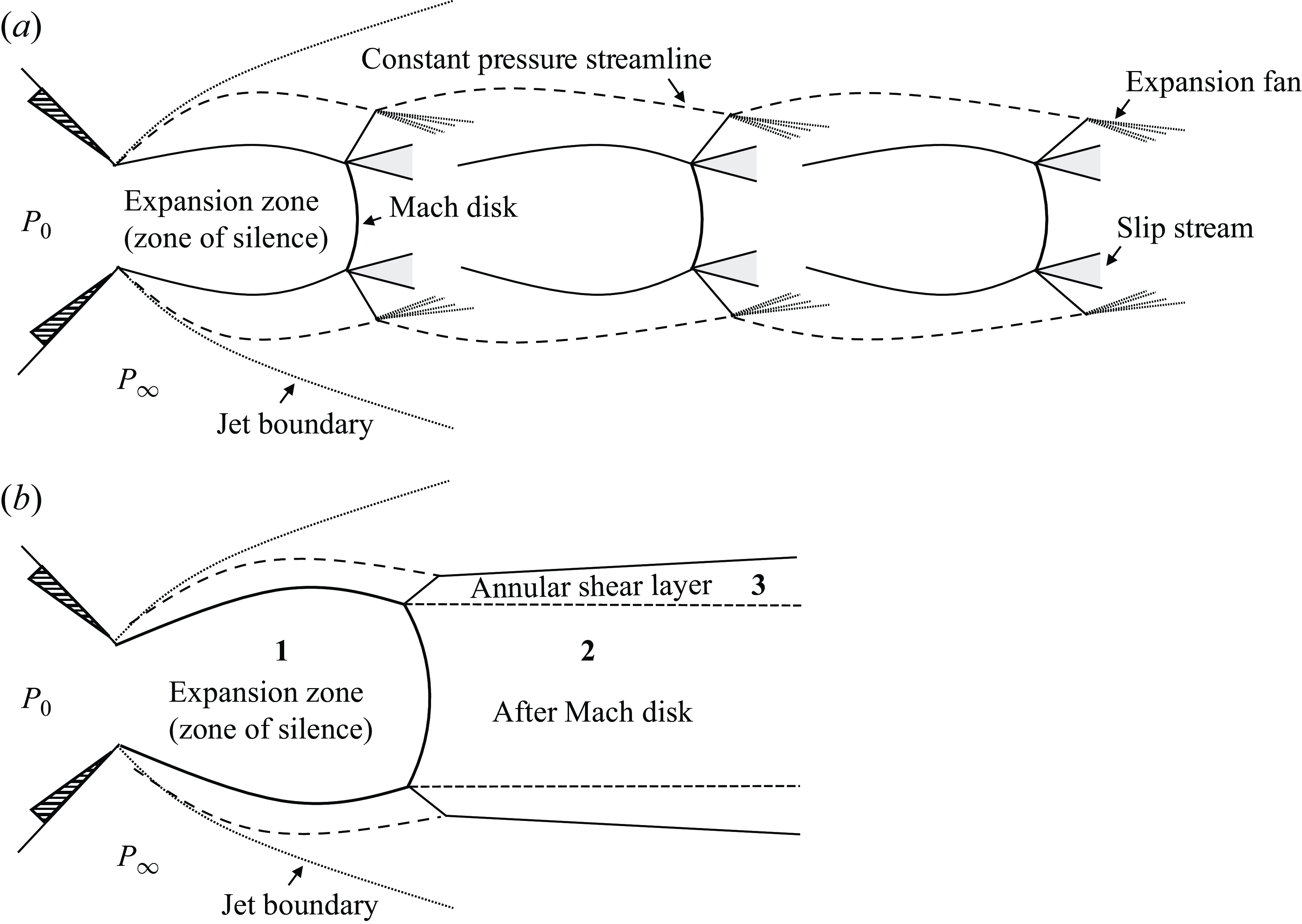
Figure 1. Schematic of flow structure in (a) a highly under-expanded and (b) an extremely under-expanded supersonic free jet.
In the over-expanded regime, the exit pressure of the jet is less than the ambient pressure. This leads to a series of compression shocks within the jet as it adjusts to the higher ambient pressure. These shocks are typically followed by expansion fans, creating a complex pattern of alternating shocks and expansions. Conversely, the under-expanded regime occurs when the exit pressure is higher than the ambient pressure. The jet undergoes expansion waves as it adjusts to the lower external pressure, resulting in a visible spreading of the flow.
The under-expanded regime can be further divided into different subdivisions based on the magnitude of the pressure difference and corresponding flow characteristics, as depicted in figure 1. The basic under-expanded condition involves a mild series of expansions as the jet slightly adjusts to achieve equilibrium with the ambient pressure. As the pressure difference becomes more pronounced, there is a shift to a moderately or highly under-expanded regime, where intense and clearly defined shock diamonds or Mach disks appear, signifying substantial pressure adjustments through strong shockwaves followed by expansion waves. The extremely under-expanded regime features a large single shock cell or a Mach disk near the nozzle exit, followed by a long potential core and highly turbulent flow that significantly spreads the jet profile as it progresses downstream. In this study, due to the high pressure difference between the jet and the rarefied environment, we focus on the highly under-expanded jet characterised by the presence of a Mach disk and cyclical structures due to oblique shockwaves, and the extremely under-expanded regime where only a single-barrel shock structure exists.
Additionally, especially in a rarefied gas environment, it is important to consider both the NPR and the jet rarefaction factor, which depends on the Reynolds, Mach and Knudsen numbers. Previous research (Volchkov et al. Reference Volchkov, Ivanov, Kislyakov, Rebrov, Sukhnev and Sharafutdinov1973; Kislyakov, Rebrov & Sharafutdinov Reference Kislyakov, Rebrov and Sharafutdinov1975; Kosov, Rebrov & Sharafutdinov Reference Kosov, Rebrov and Sharafutdinov1980; Rebrov Reference Rebrov2001; Bykov et al. Reference Bykov, Gorbachev and Fyodorov2023) highlights the fact that the Reynolds number alone is not sufficient to fully describe the flow behaviour under rarefied conditions. This has led to the conceptualisation of a complex Reynolds number (Volchkov et al. Reference Volchkov, Ivanov, Kislyakov, Rebrov, Sukhnev and Sharafutdinov1973), denoted as $\textit{Re}_{L}$
, which is defined as the Reynolds number at the nozzle throat, divided by the NPR:
$\textit{Re}_{L}$
, which is defined as the Reynolds number at the nozzle throat, divided by the NPR:
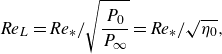 \begin{equation} \textit{Re}_{L} = \textit{Re}_{*}/\sqrt {\frac {P_{0}}{P_{\infty }}} = \textit{Re}_{*}/\sqrt {\eta _{0}}, \end{equation}
where $\textit{Re}_{*}$
is the Reynolds number based on the nozzle throat diameter,
$\textit{Re}_{*}$
is the Reynolds number based on the nozzle throat diameter, $P_{0}$
is total pressure,
$P_{0}$
is total pressure, $P_{\infty }$
is ambient pressure, and
$P_{\infty }$
is ambient pressure, and $\eta _{0}$
is the NPR, respectively. In this study,
$\eta _{0}$
is the NPR, respectively. In this study, $\textit{Re}_{*}$
was calculated using the jet velocity at the exit of the sonic nozzle, where the flow is choked. The jet velocity was determined using isentropic relations, as choking implies that the flow reaches Mach 1 at the exit. Using the known total pressure and total temperature, the static temperature under choked conditions was calculated with isentropic relations. The speed of sound, and thus the jet velocity, was then derived using the static temperature and a constant specific heat ratio. Furthermore, the corresponding complex Knudsen number (Dulov & Luk’yanov Reference Dulov and Luk’yanov1984), denoted as
$\textit{Re}_{*}$
was calculated using the jet velocity at the exit of the sonic nozzle, where the flow is choked. The jet velocity was determined using isentropic relations, as choking implies that the flow reaches Mach 1 at the exit. Using the known total pressure and total temperature, the static temperature under choked conditions was calculated with isentropic relations. The speed of sound, and thus the jet velocity, was then derived using the static temperature and a constant specific heat ratio. Furthermore, the corresponding complex Knudsen number (Dulov & Luk’yanov Reference Dulov and Luk’yanov1984), denoted as $Kn_{L}$
, is given as
$Kn_{L}$
, is given as
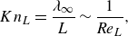 \begin{equation} Kn_{L}=\frac {\lambda _{\infty }}{L} \sim \frac {1}{\textit{Re}_{L}}, \end{equation}
where $\lambda _{\infty }$
is the mean free path of molecules in the ambient gas, and
$\lambda _{\infty }$
is the mean free path of molecules in the ambient gas, and $L$
is the characteristic length scale.
$L$
is the characteristic length scale.
The formulation of the complex Reynolds number incorporates not just the NPR but also principal parameters from key regions in the extremely under-expanded supersonic free jet, as illustrated in figure 1(b). These regions are delineated into three main areas: the zone of silence before the Mach disk (region 1), the area following the Mach disk (region 2), and the annular shear layer unaffected by the Mach disk (region 3). By calculating the Reynolds number with characteristic density, length, velocity and viscosity from each of these regions, the composite nature of the complex Reynolds number becomes evident, as detailed in Appendix A. The complex Reynolds number not only elucidates the characteristics of the near-field zone of the supersonic free jet, but also describes the far-field zone. Typically, as the jet reaches the far-field zone, it becomes fully developed, satisfying self-similarity conditions and is known to exhibit a Gaussian velocity profile.
The complex Reynolds number is used to differentiate flow characteristics, and the following distinctions represent each flow regime (Rebrov Reference Rebrov2001): turbulent for $\textit{Re}_{L}\gt 10^4$
, laminar–turbulent transition for
$\textit{Re}_{L}\gt 10^4$
, laminar–turbulent transition for $10^3\lt \textit{Re}_{L}\lt 10^4$
, laminar for
$10^3\lt \textit{Re}_{L}\lt 10^4$
, laminar for $10^2\lt \textit{Re}_{L}\lt 10^3$
, and rarefied or scattering for
$10^2\lt \textit{Re}_{L}\lt 10^3$
, and rarefied or scattering for $\textit{Re}_{L}\lt 10^2$
. The current research focuses on examining how the characteristics of the supersonic free jet change under rarefied conditions, investigating a highly under-expanded jet in the turbulent flow regime and an extremely under-expanded jet in the laminar flow regime.
$\textit{Re}_{L}\lt 10^2$
. The current research focuses on examining how the characteristics of the supersonic free jet change under rarefied conditions, investigating a highly under-expanded jet in the turbulent flow regime and an extremely under-expanded jet in the laminar flow regime.
3. Experimental set-up
3.1. Vacuum chamber
The vacuum chamber developed for this work is shown in figure 2. The cylindrical chamber dimensions are length 835 mm, outer diameter 365 mm, and inner diameter 304 mm. It features optical windows 130 mm $\times$
550 mm in size on three sides to facilitate laser illumination and excitation for PIV and MTV, respectively, and for camera imaging. In this study, a target flow rate 5 standard litres per minute and chamber pressure 1 torr were set, which is relevant to semiconductor equipment and similar to the Mars atmosphere. Two vacuum pressure gauges (numbered 2 and 3) were installed upstream and downstream to measure the internal pressure, as shown in figure 2(a). These sensors were placed sufficiently far from the jet outlet – at least 10 nozzle diameters away – to avoid disturbances caused by the jet flow. A Leybold SV-300B rotary vane vacuum pump was used in combination with a Leybold WS1001 booster to continuously evacuate the chamber. The vacuum pump was placed at the outlet with a throttle valve for pressure control. A control box adjusted the valve based on pressure readings from the gauges. Thermocouples were utilised to monitor temperature directly on the chamber walls to track ambient conditions, and upstream near the nitrogen reservoir to ensure accurate readings of total temperature. Both measurements confirmed uniform total temperature 300 K. As illustrated in figure 2(b), the nozzle is positioned 158 mm from the side optical windows, and 435 mm from the right-hand side of the window. A converging sonic nozzle with a 2 mm capillary orifice, designed per Murphy & Miller (Reference Murphy and Miller1984), was used to achieve Mach 1 at the exit. This design ensured flow stability, theoretical validation of centreline properties, and minimal wall and outlet influence on the free jet. A motorised translation stage was installed to enable movement of the entire vacuum chamber relative to the optics. It allowed for a translation range of 300 mm along the longitudinal axis, with spatial resolution 100
$\times$
550 mm in size on three sides to facilitate laser illumination and excitation for PIV and MTV, respectively, and for camera imaging. In this study, a target flow rate 5 standard litres per minute and chamber pressure 1 torr were set, which is relevant to semiconductor equipment and similar to the Mars atmosphere. Two vacuum pressure gauges (numbered 2 and 3) were installed upstream and downstream to measure the internal pressure, as shown in figure 2(a). These sensors were placed sufficiently far from the jet outlet – at least 10 nozzle diameters away – to avoid disturbances caused by the jet flow. A Leybold SV-300B rotary vane vacuum pump was used in combination with a Leybold WS1001 booster to continuously evacuate the chamber. The vacuum pump was placed at the outlet with a throttle valve for pressure control. A control box adjusted the valve based on pressure readings from the gauges. Thermocouples were utilised to monitor temperature directly on the chamber walls to track ambient conditions, and upstream near the nitrogen reservoir to ensure accurate readings of total temperature. Both measurements confirmed uniform total temperature 300 K. As illustrated in figure 2(b), the nozzle is positioned 158 mm from the side optical windows, and 435 mm from the right-hand side of the window. A converging sonic nozzle with a 2 mm capillary orifice, designed per Murphy & Miller (Reference Murphy and Miller1984), was used to achieve Mach 1 at the exit. This design ensured flow stability, theoretical validation of centreline properties, and minimal wall and outlet influence on the free jet. A motorised translation stage was installed to enable movement of the entire vacuum chamber relative to the optics. It allowed for a translation range of 300 mm along the longitudinal axis, with spatial resolution 100 $\unicode{x03BC}$
m.
$\unicode{x03BC}$
m.
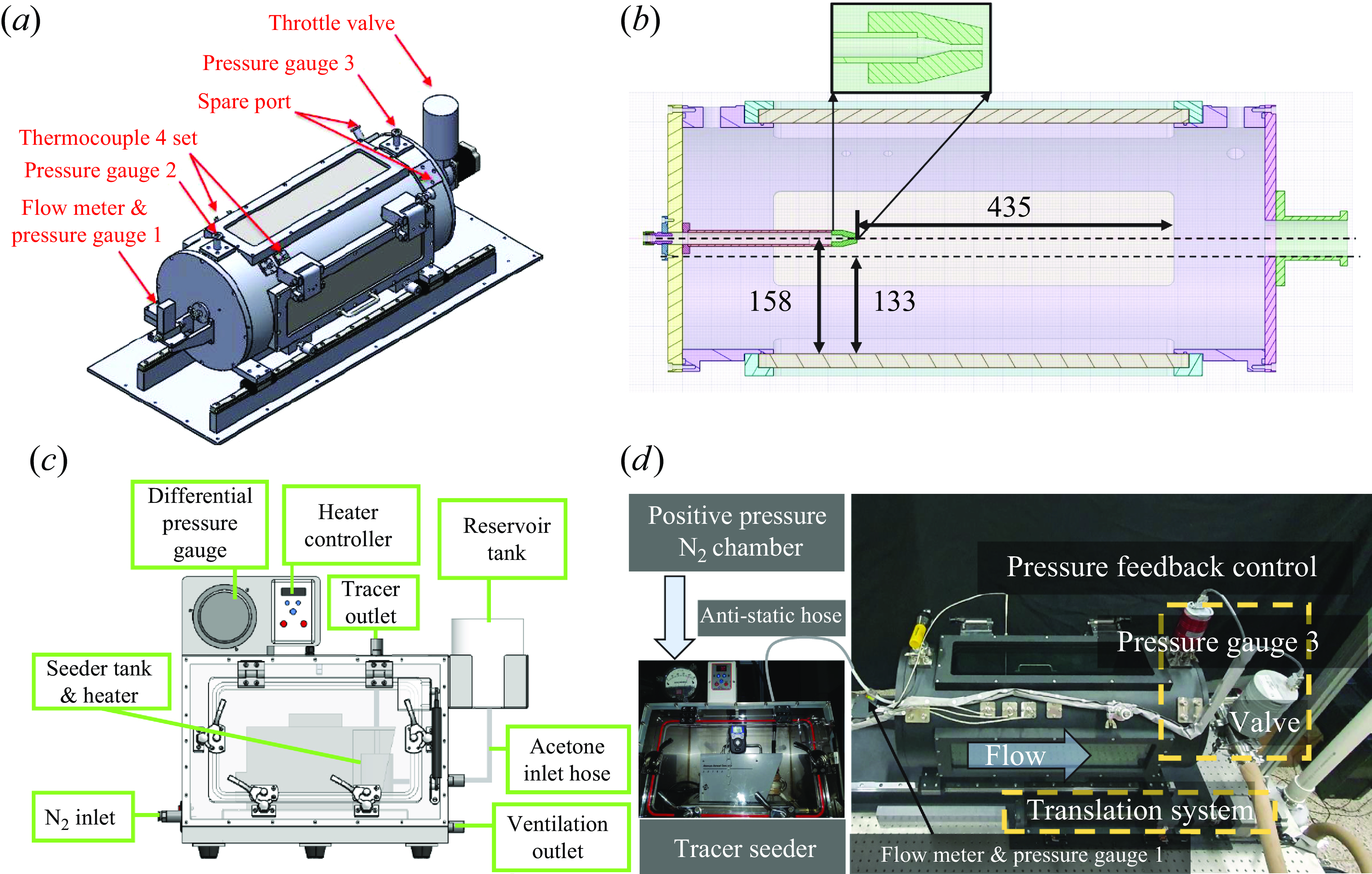
Figure 2. Experimental set-up: (a) vacuum chamber, (b) top view cross-section of vacuum chamber (measurements in mm), (c) tracer seeder within positive pressure $\mathrm{N_{2}}$
chamber, (d) overall system.
$\mathrm{N_{2}}$
chamber, (d) overall system.
However, due to the sudden pressure drop that occurs in the expansion zone near the sonic nozzle outlet, an additional pressure gauge 1 (SMC ZSE30AF-01-C) and flow meter (SMC PFM710S-01-D) were installed between the chamber and the tracer seeder to determine total pressure and flow rate, respectively, as shown in figure 2(a). The total pressure was measured using upstream pressure gauge 1, located before the flow entered the chamber, ensuring an accurate total pressure measurement unaffected by chamber dynamics.
A positive pressure $\mathrm{N_{2}}$
chamber was installed adjacent to the vacuum chamber to facilitate tracer seeding, thereby removing the possibility for
$\mathrm{N_{2}}$
chamber was installed adjacent to the vacuum chamber to facilitate tracer seeding, thereby removing the possibility for $\mathrm{O_{2}}$
quenching of phosphorescence in the MTV experiments, and ensuring that large external particles do not enter the seeder in the PIV experiments. As shown in figure 2(c), the
$\mathrm{O_{2}}$
quenching of phosphorescence in the MTV experiments, and ensuring that large external particles do not enter the seeder in the PIV experiments. As shown in figure 2(c), the $\mathrm{N_{2}}$
chamber features an inlet for ultra-pure dry
$\mathrm{N_{2}}$
chamber features an inlet for ultra-pure dry $\mathrm{N_{2}}$
to enter. The seeder was a TSI aerosol generator (model 3079A) for injecting NaCl nano-particles for PIV, and acetone nano-droplets for MTV. Additionally, a side reservoir tank was equipped to continuously supply fluid to the seeder tank. To ensure temperature stability after acetone vaporisation cooling, the seeder tank was heated and controlled by a heater controller. An
$\mathrm{N_{2}}$
to enter. The seeder was a TSI aerosol generator (model 3079A) for injecting NaCl nano-particles for PIV, and acetone nano-droplets for MTV. Additionally, a side reservoir tank was equipped to continuously supply fluid to the seeder tank. To ensure temperature stability after acetone vaporisation cooling, the seeder tank was heated and controlled by a heater controller. An $\mathrm{O_{2}}$
sensor was installed inside the positive pressure
$\mathrm{O_{2}}$
sensor was installed inside the positive pressure $\mathrm{N_{2}}$
chamber to verify that the
$\mathrm{N_{2}}$
chamber to verify that the $\mathrm{O_{2}}$
concentration was negligible. Connections between the chambers used anti-static hoses to prevent particle agglomeration. The overall configuration of the vacuum chamber and pump set-up is shown in figure 2(d). The overall experimental conditions are detailed in table 1. The fluid thermophysical properties required for calculating these parameters were obtained from the NIST Standard Reference Database (Linstrom et al. 2005), with detailed information provided in Appendix B.
$\mathrm{O_{2}}$
concentration was negligible. Connections between the chambers used anti-static hoses to prevent particle agglomeration. The overall configuration of the vacuum chamber and pump set-up is shown in figure 2(d). The overall experimental conditions are detailed in table 1. The fluid thermophysical properties required for calculating these parameters were obtained from the NIST Standard Reference Database (Linstrom et al. 2005), with detailed information provided in Appendix B.
Table 1. Overall experimental conditions.
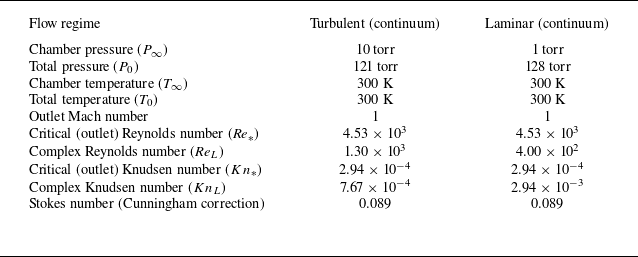
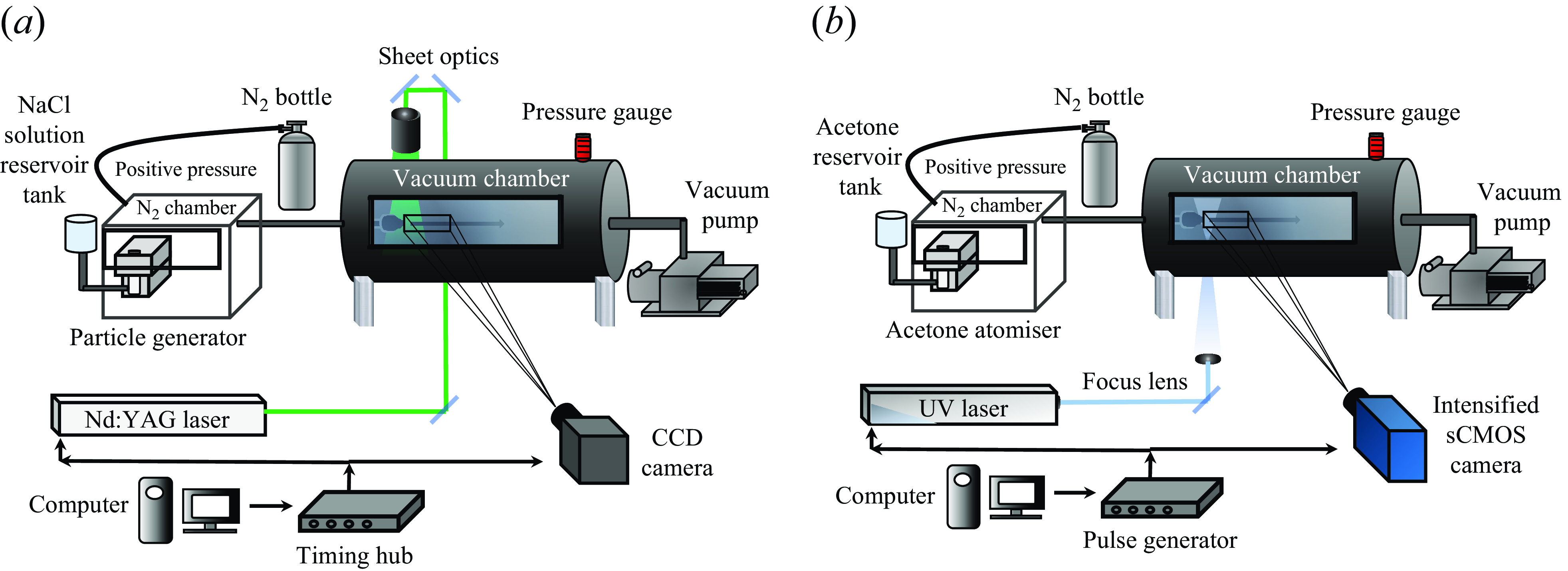
Figure 3. Experimental set-up for (a) PIV and (b) MTV and LIF.
3.2. Particle image velocimetry (PIV)
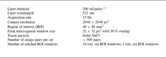
A schematic of the set-up for the PIV experiments is shown in figure 3(a). The system consisted of a dual-cavity 200 $\text{mJ}\ \text{pulse}^{-1}$
532 nm Nd:YAG laser with frequency 15 Hz. The laser sheet was oriented such that it passed vertically through the vacuum chamber. Images were acquired using a dual-frame 12 bit CCD camera (VH-4MC-M20A0) with 2048
$\text{mJ}\ \text{pulse}^{-1}$
532 nm Nd:YAG laser with frequency 15 Hz. The laser sheet was oriented such that it passed vertically through the vacuum chamber. Images were acquired using a dual-frame 12 bit CCD camera (VH-4MC-M20A0) with 2048 $\times$
2048 pixel
$\times$
2048 pixel $^{2}$
equipped with a 105 mm macro lens at f/2.8, for a region of interest (ROI) measuring 40
$^{2}$
equipped with a 105 mm macro lens at f/2.8, for a region of interest (ROI) measuring 40 $\times$
40 mm
$\times$
40 mm $^{2}$
. The vacuum chamber was capable of longitudinal movement up to 300 mm, which allowed for precise selection of the measurement region. Image stitching was employed to obtain an aggregate overall velocity field.
$^{2}$
. The vacuum chamber was capable of longitudinal movement up to 300 mm, which allowed for precise selection of the measurement region. Image stitching was employed to obtain an aggregate overall velocity field.
The PIV flow tracers were NaCl particles, chosen for their low ( $\sim0.5{\times}$
) density compared to other solid tracer particles. Nano-particles were generated using a 0.001 mol aqueous solution of NaCl in the aerosol generator. These particles were atomised into droplets, which upon evaporation left NaCl solutes that were used as seed particles. Sufficient length of the tube leading into the vacuum chamber was ensured to allow complete evaporation of the droplets into NaCl particles. The size distribution of these particles was diagnosed using a TSI scanning mobility particle sizer (SMPS) model 3938, and the results are given in figure 4. The average size of the particles was approximately 40 nm.
$\sim0.5{\times}$
) density compared to other solid tracer particles. Nano-particles were generated using a 0.001 mol aqueous solution of NaCl in the aerosol generator. These particles were atomised into droplets, which upon evaporation left NaCl solutes that were used as seed particles. Sufficient length of the tube leading into the vacuum chamber was ensured to allow complete evaporation of the droplets into NaCl particles. The size distribution of these particles was diagnosed using a TSI scanning mobility particle sizer (SMPS) model 3938, and the results are given in figure 4. The average size of the particles was approximately 40 nm.
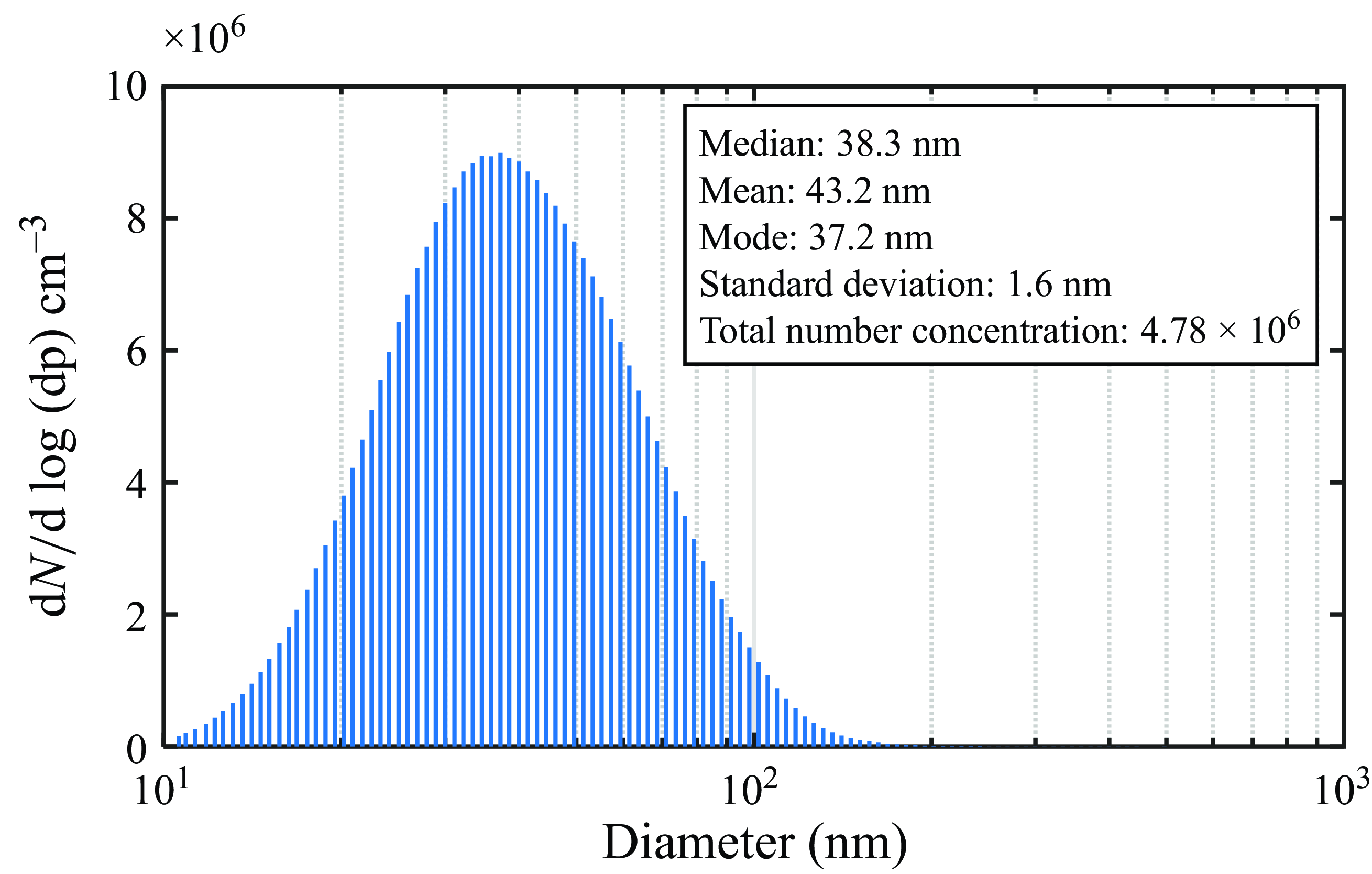
Figure 4. The NaCl solid particle size distribution.
Considering the particle size, which is smaller than the laser wavelength, the scattering regime can be classified as Rayleigh scattering rather than Mie scattering. These particles act as a solid-phase carrier within the nitrogen gas phase. Due to their size and composition, the scattering intensity from the nano-particles is several orders of magnitude greater than that of the surrounding nitrogen. Consequently, the primary signal captured by the camera is dominated by the nano-particles. The captured signal distributions closely resemble typical PIV images rather than those of molecular Rayleigh scattering.
The time interval between successive PIV images was controlled using an IDT MotionPro timing hub that has 100 ns temporal resolution, and was adjusted according to the free jet velocity. Nanosecond intervals were used in the near-field zone (i.e. a high-speed region), while microsecond intervals were used in the far-field zone where the velocity was decaying. Over 500 image pairs were captured for each ROI and analysed using PIVlab (Stamhuis & Thielicke Reference Stamhuis and Thielicke2014). The final interrogation window size was 32 $\times$
32 pixel
$\times$
32 pixel $^{2}$
with 50 % overlap due to the wide dynamic range of velocity. All experimental parameters related to the PIV set-up are summarised in table 2.
$^{2}$
with 50 % overlap due to the wide dynamic range of velocity. All experimental parameters related to the PIV set-up are summarised in table 2.
Table 2. The PIV system parameters.
3.3. Molecular tagging velocimetry (MTV) and laser-induced fluorescence (LIF)
The MTV technique does not rely on tracer particles but directly measures the flow velocity using gas molecules. This method inherently avoids issues related to flow traceability present in PIV, as it measures velocity not indirectly through tracer particles, but directly through gas molecules. Common tracer molecules include acetone, biacetyl and toluene, which are used based on their emission characteristics and the environmental conditions of the experiment. In this study, acetone was utilised.
The basic MTV measurement method seeds the molecular tracers into the flow. When exposed to an appropriate ultraviolet (UV) laser, acetone molecules undergo excitation, and emit light at a different wavelength when returning to the ground state. This light emission can occur in two forms: fluorescence and phosphorescence. Fluorescence occurs in extremely short times of the order of nanoseconds, but with high intensity, followed by a longer-lasting, lower-intensity phosphorescence. This emission characteristic has been used extensively in rarefied supersonic free jets, with early applications by Lempert et al. (Reference Lempert, Jiang, Sethuram and Samimy2002). The emitted light from the tracer molecules is captured using a high-sensitivity camera recording images at predetermined intervals. By analysing the recorded images as shown in figure 5, the displacement of the tracer molecules over known time intervals can be observed. Lines are drawn in the streamwise direction to perform Gaussian fitting, with the velocity determined based on distance moved of the Gaussian profile peak, as depicted in figure 6(a).
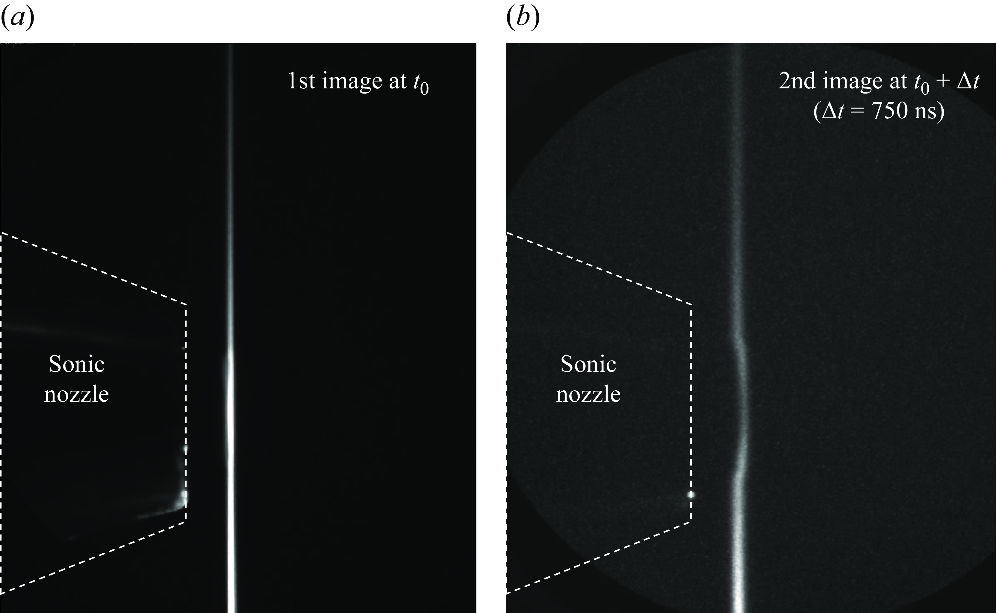
Figure 5. Example of successive MTV images at 1 torr: (a) first image, and (b) second image.
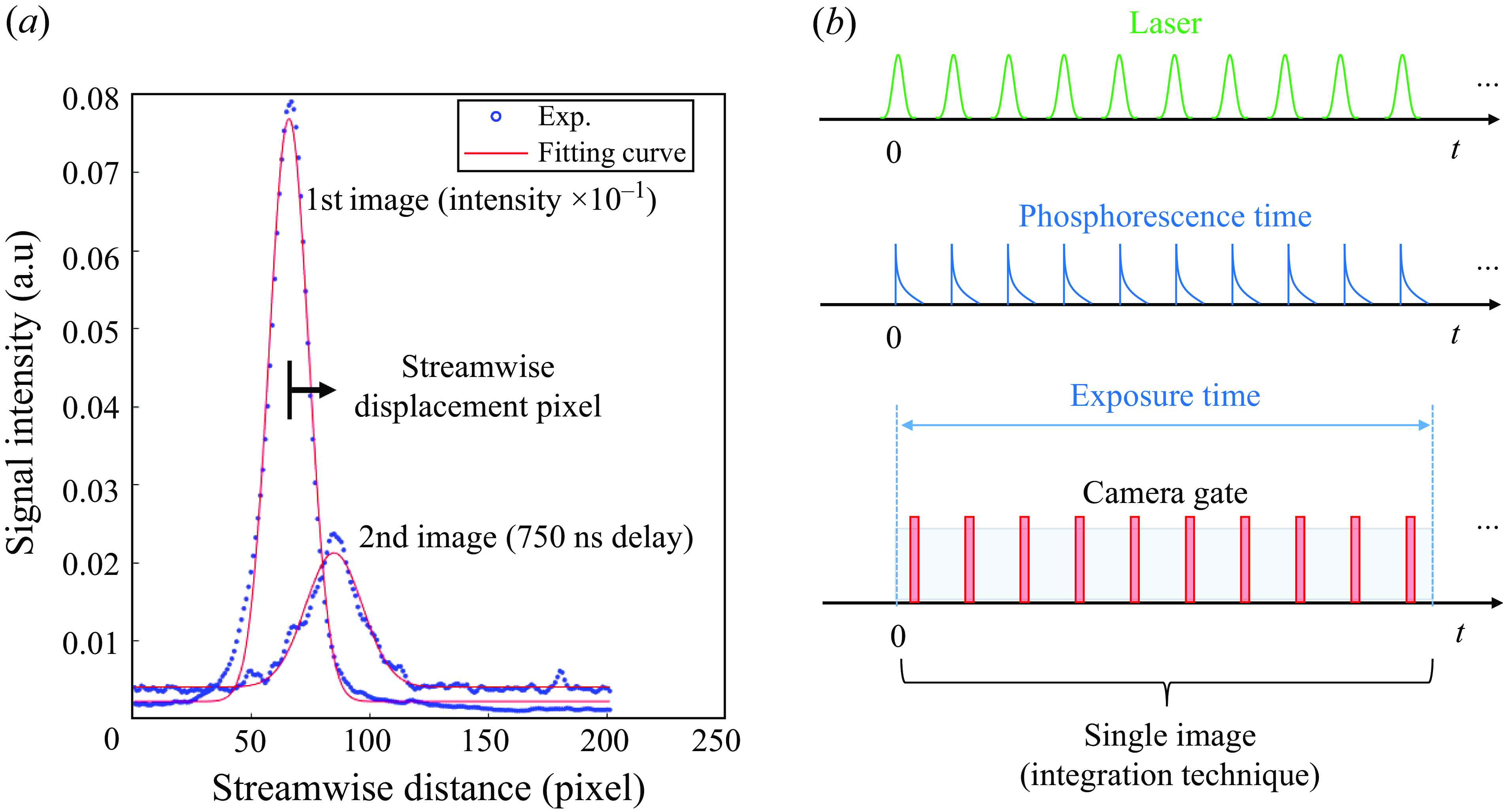
Figure 6. (a) Signal intensity of first image (downscaled by $10^{-1}$
for visibility) and second image with Gaussian fitting. (b) Signal sequence of MTV using integration technique.
$10^{-1}$
for visibility) and second image with Gaussian fitting. (b) Signal sequence of MTV using integration technique.
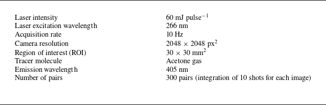
For the MTV experimental set-up, as illustrated in figure 3(b), the same chamber used for PIV was employed. The system consisted of a 60 mJ UV single-pulse laser at 266 nm with frequency 10 Hz. This change was necessary to induce the desired molecular excitation in acetone. It should be noted that the energy output of the lasers (both PIV and MTV) was routinely monitored using optical power meters (Thorlabs PM400 and S470C, respectively) to ensure stability across experiments.
Gaseous acetone was used as the molecular tracer, and was introduced using the same aerosol generator as in the PIV experiment. Upon UV irradiation, both fluorescence and phosphorescence emission at wavelength 405 nm were detected. An intensified 16 bit sCMOS camera (Excelitas pco.dicam C1 P46) was employed with 2048 $\times$
2048 pixel
$\times$
2048 pixel $^{2}$
equipped with a 200 mm macro lens at f/4, and focused on an ROI measuring 30
$^{2}$
equipped with a 200 mm macro lens at f/4, and focused on an ROI measuring 30 $\times$
30 mm
$\times$
30 mm $^{2}$
. The camera integration technique developed by Fratantonio et al. (Reference Fratantonio, Rojas-Cardenas, Mohand, Barrot, Baldas and Colin2018, Reference Fratantonio, Rojas-Cárdenas, Barrot, Baldas and Colin2020) was used in this work. As illustrated in figure 6(b), this technique allows for the capture of light generated by multiple laser excitations in a single image by keeping the camera gate open for a specified duration after each laser irradiation. This method enhanced the signal-to-noise ratio (SNR) by allowing the accumulation of 10 shots per image, synchronised with the 10 Hz frequency of the pulsed UV laser in this experiment.
$^{2}$
. The camera integration technique developed by Fratantonio et al. (Reference Fratantonio, Rojas-Cardenas, Mohand, Barrot, Baldas and Colin2018, Reference Fratantonio, Rojas-Cárdenas, Barrot, Baldas and Colin2020) was used in this work. As illustrated in figure 6(b), this technique allows for the capture of light generated by multiple laser excitations in a single image by keeping the camera gate open for a specified duration after each laser irradiation. This method enhanced the signal-to-noise ratio (SNR) by allowing the accumulation of 10 shots per image, synchronised with the 10 Hz frequency of the pulsed UV laser in this experiment.
Unlike in PIV, which captures nano-particle Rayleigh scattering, shutter speed is important for MTV due to the duration of phosphorescence, which is of the order of microseconds. To prevent image streaking and reduce measurement uncertainty, camera gate time 20 ns was used, which is approximately an order of magnitude shorter than the expected phosphorescence duration. This gate time was achieved using a pulse generator (Quantum Composers 9528) with temporal resolution 250 ps. The sequence of UV laser exposure was verified using a 1 ns rise time photodiode (Thorlabs SM05PD2A), connected to a 1 GHz bandwidth oscilloscope (Teledyne LeCroy Wavesurfer 510), to ensure correct timing. A total of 300 image pairs per set were captured using this method. The specific experimental parameters related to the MTV setup are summarised in table 3.
Table 3. The MTV system parameters.
To further elucidate the shockwave structure of the supersonic free jet, acetone LIF was utilised – LIF is particularly effective for visualising shockwave structures because fluorescence intensity is proportional to the acetone concentration, allowing the identification of high-concentration regions within shockwaves (Tropea et al. Reference Tropea, Yarin and Foss2007; Inman et al. Reference Inman, Danehy, Nowak and Alderfer2008; Yu et al. Reference Yu, Vuorinen, Kaario, Sarjovaara and Larmi2013). Unlike MTV, which requires two images for analysis, LIF can be analysed with a single image, making it a more straightforward method. To visualise a wider area, the laser beam is expanded into a broad sheet rather than focused into a single point. This adjustment is easily achieved by replacing the focusing lens used in MTV with a lens that creates a planar laser sheet.
3.4. Measurement uncertainty analysis
Measurement uncertainty is an inherent aspect of any experimental technique, requiring a comprehensive analysis of its sources to ensure reliable results. In this study, the Guide to the Expression of Uncertainty in Measurement (GUM) framework (ISO, OIML & BIPM 2009) was utilised to calculate standard uncertainty by identifying influencing factors, evaluating Type A (random) and Type B (bias) uncertainties, and determining the combined standard uncertainty. Consideration of the correlation between elements and their respective sensitivity coefficients was essential, using the root sum of squares method for independent elements. Finally, the extended uncertainty is obtained by multiplying the combined uncertainty by an appropriate coverage factor ( $k$
) to account for the level of confidence.
$k$
) to account for the level of confidence.
3.4.1. The PIV uncertainty analysis
The ability of tracer particles to follow the flow in PIV applications, particularly in supersonic free jets, is typically verified using the Stokes number. Traditionally, the Stokes number is calculated at the nozzle outlet, which serves as a reference point for flow characterisation because it typically exhibits the highest velocity in incompressible free jets, and the highest Stokes number (which presents the worst condition for particle tracking). However, in compressible flows such as supersonic free jets, the flow velocity increases further beyond the nozzle outlet in the transient expansion region, particularly before the Mach disk in the first shock cell. This highlights the need for more nuanced approaches when analysing compressible flows under rarefied conditions. In this study, the Stokes number is calculated at the nozzle outlet, similar to previous studies in supersonic free jets (De Gregorio Reference De Gregorio2014; Edgington-Mitchell et al. Reference Edgington-Mitchell, Oberleithner, Honnery and Soria2014b ). However, we further investigated the downstream evolution of the Stokes number, particularly within the zone of silence, where rapid density decreases significantly affect particle traceability (refer to Appendix C).
Measurement uncertainty in PIV, which has been extensively studied in previous research (Sciacchitano & Wieneke Reference Sciacchitano and Wieneke2016; Sciacchitano Reference Sciacchitano2019), depends on the magnification factor $M$
, time interval
$M$
, time interval $\Delta t$
, and pixel displacement
$\Delta t$
, and pixel displacement $\Delta s$
, which determine the velocity of tracer particles. It is critical that particles adequately follow the flow, a condition assumed if the corrected Stokes number is significantly less than unity. Before calculating these uncertainties, image distortion was carefully addressed to ensure accuracy in the measurements. Perspective error, which can arise from optical distortion caused by wide-angle lenses, was minimised by using a small ROI and verifying alignment with a reference object placed in the light sheet plane. Particle image sizes were compared between the centre and edges of the frame to confirm the absence of significant distortion, and depth of field checks ensured that all particles within the laser sheet were in focus. Additionally, the vacuum chamber was translated during set-up to maintain optical alignment. Once image distortion was confirmed to be negligible, the standard uncertainty of the magnification factor is measured by the pixel resolution, using a triangular probability distribution based on the maximum and minimum values of the image of a ruler placed in the light sheet plane prior to the PIV measurements. Similarly, the standard uncertainty of the time interval is derived from the temporal resolution of the timing hub, as specified by the manufacturer, employing a rectangular probability distribution. The standard uncertainty of pixel displacement was set at 0.1 pixel, made feasible by the use of nano-particle-based Rayleigh scattering. These uncertainties are combined, and a coverage factor
$\Delta s$
, which determine the velocity of tracer particles. It is critical that particles adequately follow the flow, a condition assumed if the corrected Stokes number is significantly less than unity. Before calculating these uncertainties, image distortion was carefully addressed to ensure accuracy in the measurements. Perspective error, which can arise from optical distortion caused by wide-angle lenses, was minimised by using a small ROI and verifying alignment with a reference object placed in the light sheet plane. Particle image sizes were compared between the centre and edges of the frame to confirm the absence of significant distortion, and depth of field checks ensured that all particles within the laser sheet were in focus. Additionally, the vacuum chamber was translated during set-up to maintain optical alignment. Once image distortion was confirmed to be negligible, the standard uncertainty of the magnification factor is measured by the pixel resolution, using a triangular probability distribution based on the maximum and minimum values of the image of a ruler placed in the light sheet plane prior to the PIV measurements. Similarly, the standard uncertainty of the time interval is derived from the temporal resolution of the timing hub, as specified by the manufacturer, employing a rectangular probability distribution. The standard uncertainty of pixel displacement was set at 0.1 pixel, made feasible by the use of nano-particle-based Rayleigh scattering. These uncertainties are combined, and a coverage factor $k\approx2$
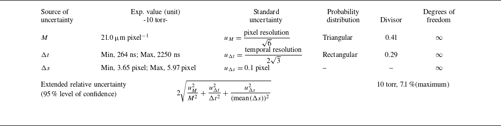
for 95 % level of confidence is applied to determine the extended uncertainty. In this study, specific uncertainties arising from shockwaves and Rayleigh-scattering-induced optical distortions due to steep flow property (e.g. density or temperature) gradients were not considered, as the main quantitative PIV analysis was conducted in the far-field zone where these issues are not prominent. The maximum overall uncertainty of PIV is 7.1 % in a highly under-expanded regime, with the detailed uncertainty budget presented in table 4.
$k\approx2$
for 95 % level of confidence is applied to determine the extended uncertainty. In this study, specific uncertainties arising from shockwaves and Rayleigh-scattering-induced optical distortions due to steep flow property (e.g. density or temperature) gradients were not considered, as the main quantitative PIV analysis was conducted in the far-field zone where these issues are not prominent. The maximum overall uncertainty of PIV is 7.1 % in a highly under-expanded regime, with the detailed uncertainty budget presented in table 4.
Table 4. The PIV uncertainty budget.
Notes: The PIV uncertainty at 1 torr was omitted due to inconsistencies in both near-field and far-field zones.
Table 5. The MTV uncertainty budget.
(*) Standard uncertainty of $u_{\Delta y}$
was accounted for at different locations when calculating the combined uncertainty, yielding the maximum value.
$u_{\Delta y}$
was accounted for at different locations when calculating the combined uncertainty, yielding the maximum value.
3.4.2. The MTV uncertainty analysis
Unlike PIV, where uncertainty sources are well documented, MTV uncertainty remains less studied, with early applications identifying factors such as flow unsteadiness and image degradation. While consensus on estimation methods is lacking, recent efforts have advanced quantification. In this study, we applied the latest analytical methods to assess MTV uncertainty (Pitz & Danehy Reference Pitz and Danehy2020).
In our investigation, MTV is employed in a one-dimensional fashion focusing solely on measuring streamwise velocity. Consequently, the standard uncertainty associated with factors such as magnification factor and time interval aligns with that of PIV. However, MTV has an additional source of uncertainty related to spanwise velocity assumptions, as elucidated in Mustafa et al. (Reference Mustafa, Parziale, Smith and Marineau2017). Typically, this entails assuming an uncertainty equivalent to 5 % of the freestream velocity. For our analysis, we assume the velocity beyond the main jet to represent the freestream velocity. The uncertainty in streamwise pixel displacement was determined based on previous studies (Gendrich & Koochesfahani Reference Gendrich and Koochesfahani1996; Ramsey & Pitz Reference Ramsey and Pitz2011). The accuracy of determining streamwise pixel displacements relies on precise Gaussian fitting, assessed quantitatively through the SNR, defined as
 \begin{equation} \text{SNR}=\frac {S_p}{4\sigma _N}, \end{equation}
where $S_{p}$
represents the peak intensity obtained from Gaussian fitting, while
$S_{p}$
represents the peak intensity obtained from Gaussian fitting, while $\sigma _{N}$
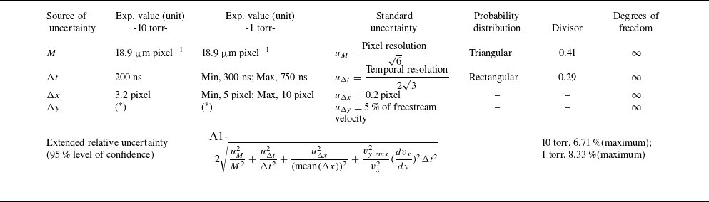
signifies the standard deviation of noise, which comes from the residual values after the Gaussian fit is subtracted from the experimental data. Through the SNR, the accuracy of Gaussian fitting can be assessed, facilitating the quantification of uncertainty in pixel displacement. When the SNR exceeds 4, the uncertainty in pixel displacement is typically approximately 0.2 pixel considering the laser linewidth. For instance, as depicted in figure 7(a), the first image exhibits a high SNR at 11.6, indicating precise peak identification. Conversely, in subsequent shots such as the delayed second image, both emission intensity and SNR decrease. However, despite the decrement, the peaks still exhibit sufficient reliability, as shown in figure 7(b). On the contrary, in cases such as figure 7(c) with a lower SNR, the uncertainty in pixel displacement increases significantly, rendering the data unsuitable for velocity calculation. Such data were excluded from our analysis, with calculations performed only on Gaussian fits with SNR exceeding 4. The maximum overall uncertainties of MTV are 6.71 % in a highly under-expanded regime, and 8.33 % in an extremely under-expanded regime, as detailed in table 5.
$\sigma _{N}$
signifies the standard deviation of noise, which comes from the residual values after the Gaussian fit is subtracted from the experimental data. Through the SNR, the accuracy of Gaussian fitting can be assessed, facilitating the quantification of uncertainty in pixel displacement. When the SNR exceeds 4, the uncertainty in pixel displacement is typically approximately 0.2 pixel considering the laser linewidth. For instance, as depicted in figure 7(a), the first image exhibits a high SNR at 11.6, indicating precise peak identification. Conversely, in subsequent shots such as the delayed second image, both emission intensity and SNR decrease. However, despite the decrement, the peaks still exhibit sufficient reliability, as shown in figure 7(b). On the contrary, in cases such as figure 7(c) with a lower SNR, the uncertainty in pixel displacement increases significantly, rendering the data unsuitable for velocity calculation. Such data were excluded from our analysis, with calculations performed only on Gaussian fits with SNR exceeding 4. The maximum overall uncertainties of MTV are 6.71 % in a highly under-expanded regime, and 8.33 % in an extremely under-expanded regime, as detailed in table 5.
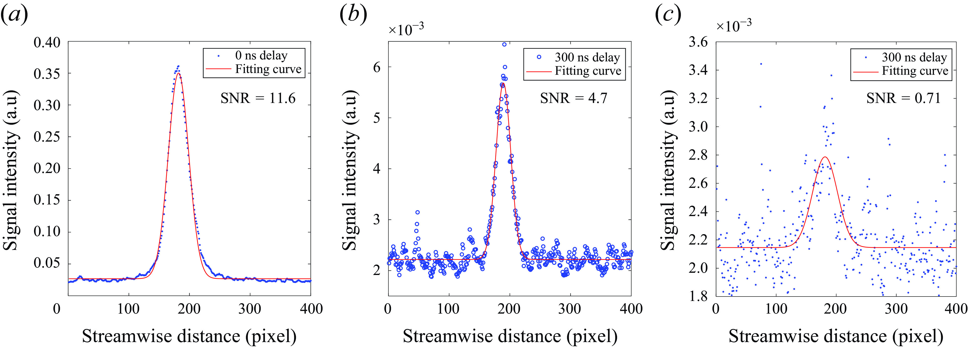
Figure 7. Signal intensity of (a) first image, (b) second image with Gaussian fitting for high SNR, and (c) second image with Gaussian fitting at low SNR.
4. Results and discussion
4.1. Highly under-expanded supersonic free jet (turbulent flow regime)
4.1.1. Shockwave structure
The LIF was performed to visualise the shockwave structure of the supersonic free jet under the conditions listed in table 1. The LIF image shown in figure 8(a) was obtained by ensemble averaging 100 individual images using an integration technique. This approach averages out fluctuations and highlights the overall flow characteristics. Figure 8(a) illustrates the presence of oblique shocks and a Mach disk at the outlet, along with a cyclical wake structure that shows a highly under-expanded regime within the supersonic free jet. This visualisation closely resembles observations of shockwave structures in supersonic free jets at atmospheric pressure, as depicted in figure 8(b).
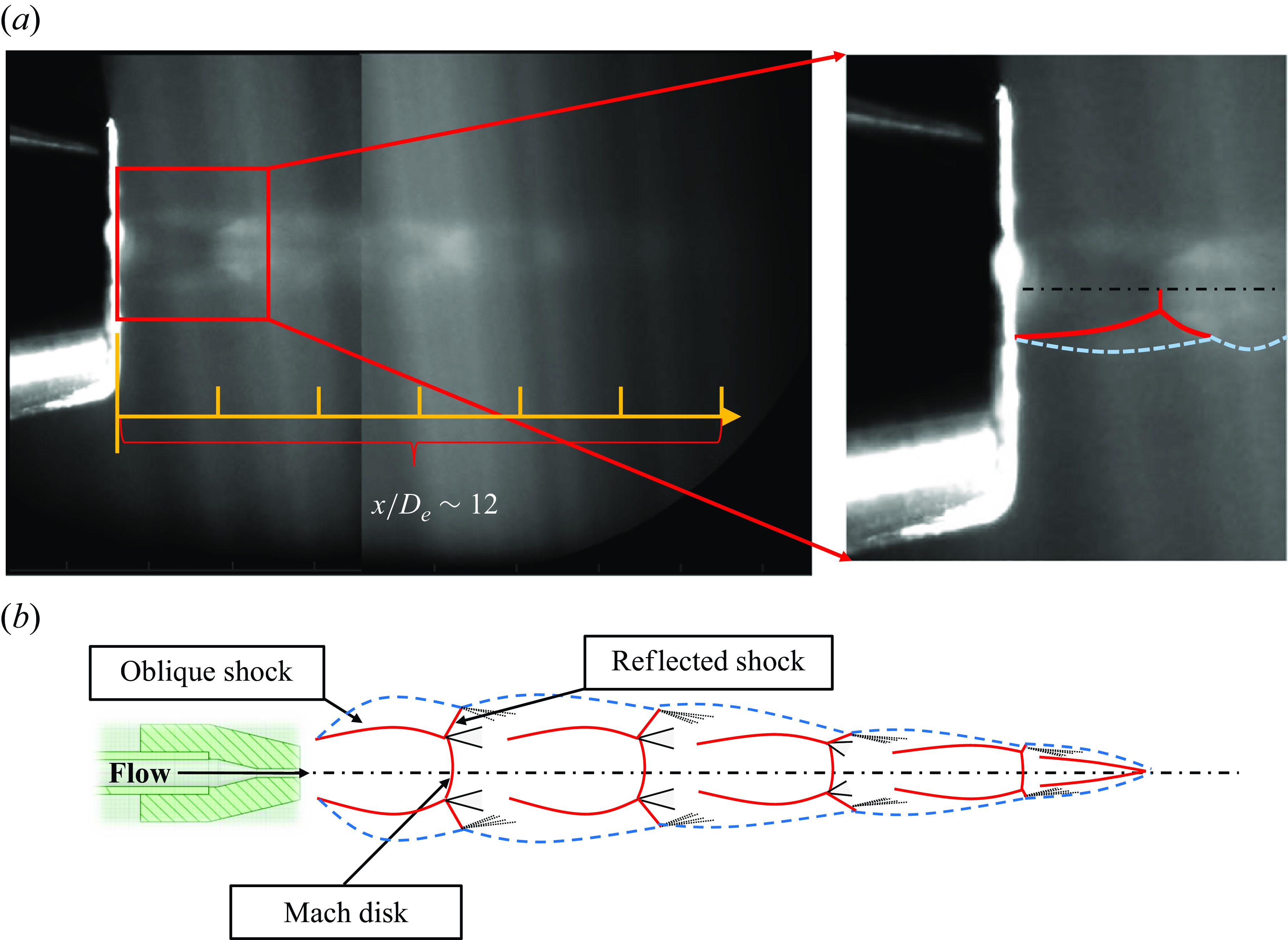
Figure 8. Combined LIF field of view for highly under-expanded supersonic free jet: (a) cyclical shockwave structure in the near-field zone where the axial distance has been normalised by the nozzle diameter ( $D_e$
), and (b) schematic of flow structure.
$D_e$
), and (b) schematic of flow structure.
4.1.2. Near-field zone
In a jet, velocity remains constant in the potential core before decaying in the fully developed region, forming a Gaussian profile. Consequently, centreline velocity is commonly used to assess jet behaviour. However, in supersonic jets, oblique and normal shockwaves disrupt this pattern, preventing a uniform or Gaussian profile. The normal shockwave notably reduces velocity, making the centreline velocity lower than the surrounding flow. Therefore, in supersonic jets, both centreline and maximum velocities were evaluated to capture the jet’s overall characteristics. Figure 9 presents the axial variation of the centreline and maximum streamwise velocity, where the axial distance has been normalised by the nozzle diameter. Similarly figure 10 presents the radial variation of streamwise velocity at selected axial locations. Again, the radial distance has been normalised by the nozzle diameter. Notably, there are substantial disparities between PIV and MTV measurements in the near-field zone. Initial variations between MTV and PIV likely stem from the influence of free expansion and shockwaves, while measurements downstream show converging values.
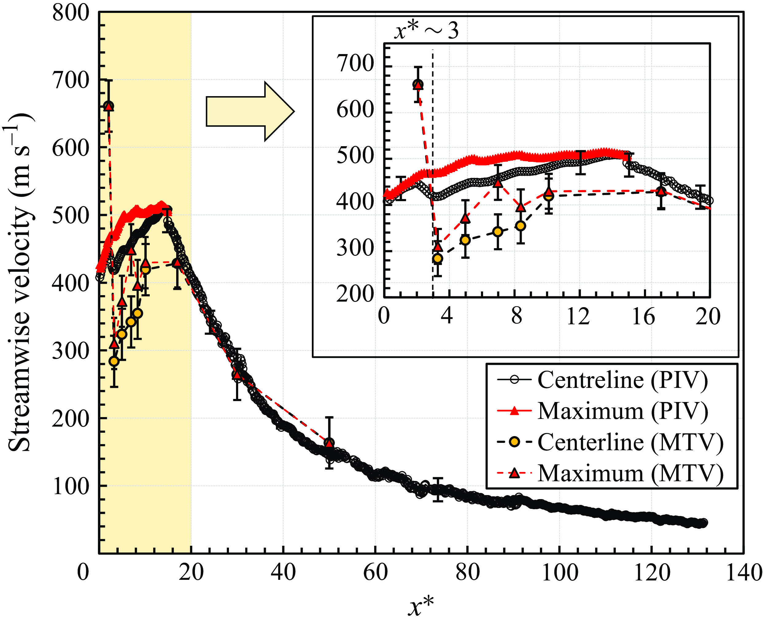
Figure 9. Evolution of centreline and maximum streamwise mean velocities from PIV and MTV.
Figure 9 suggests that in the near-field zone, PIV tracer particles generally fail to follow the flow accurately. After exiting at Mach 1 ( $\sim320\ \text{m}\ \text{s}^{-1}$
) from the sonic nozzle, the velocity increases as it passes through the first expansion zone, which is a continuum region without shockwaves (figure 1). The PIV shows an initial increase in velocity in this expansion zone, but MTV cannot do so due to laser sheet thickness limits, leading to light reflections from the nozzle that introduce noise and obscure measurements, especially in highly under-expanded supersonic jets with small shockwave structures. Both results suddenly decrease at
$\sim320\ \text{m}\ \text{s}^{-1}$
) from the sonic nozzle, the velocity increases as it passes through the first expansion zone, which is a continuum region without shockwaves (figure 1). The PIV shows an initial increase in velocity in this expansion zone, but MTV cannot do so due to laser sheet thickness limits, leading to light reflections from the nozzle that introduce noise and obscure measurements, especially in highly under-expanded supersonic jets with small shockwave structures. Both results suddenly decrease at $x/D_{{e}} \sim3$
after the Mach disk. The reduction in velocity is significantly more pronounced in MTV than in PIV. After this decrease, PIV shows a slight steady increase, while MTV shows a stronger increase. This discrepancy suggests that PIV particles may not effectively follow the rapid changes in velocity and flow gradients through the shockwave zone. Additionally, Rayleigh scattering effects, particularly in regions of large temperature and density gradients, may influence the PIV measurements.
$x/D_{{e}} \sim3$
after the Mach disk. The reduction in velocity is significantly more pronounced in MTV than in PIV. After this decrease, PIV shows a slight steady increase, while MTV shows a stronger increase. This discrepancy suggests that PIV particles may not effectively follow the rapid changes in velocity and flow gradients through the shockwave zone. Additionally, Rayleigh scattering effects, particularly in regions of large temperature and density gradients, may influence the PIV measurements.
To observe more detailed velocity changes, we compared streamwise mean velocities from MTV and PIV at various positions in the near-field zone after the Mach disk (figure 10). Both experiments show similar profile shapes, but MTV reports significantly lower velocities, especially at $x/D_{{e}} = 3.29$
. This difference is due to the velocity reduction after the shockwave which the PIV tracer particles cannot sufficiently resolve. Furthermore, instead of a Gaussian distribution jet profile, a dual-peak velocity profile exists, due to influence from the Mach disk. The Mach disk is generally considered a normal shockwave with low pressure difference. However, when there is a significant pressure difference, curvature occurs, causing only the central part to behave as a normal shockwave, while the surrounding areas experience a weaker shock. This results in significant velocity reduction at the centre, with less reduction in the surrounding regions, leading to a dual-peak velocity profile. Both MTV and PIV show an increase in velocity downstream after the Mach disk, with velocities in the centre region increasing due to the favourable pressure gradient.
$x/D_{{e}} = 3.29$
. This difference is due to the velocity reduction after the shockwave which the PIV tracer particles cannot sufficiently resolve. Furthermore, instead of a Gaussian distribution jet profile, a dual-peak velocity profile exists, due to influence from the Mach disk. The Mach disk is generally considered a normal shockwave with low pressure difference. However, when there is a significant pressure difference, curvature occurs, causing only the central part to behave as a normal shockwave, while the surrounding areas experience a weaker shock. This results in significant velocity reduction at the centre, with less reduction in the surrounding regions, leading to a dual-peak velocity profile. Both MTV and PIV show an increase in velocity downstream after the Mach disk, with velocities in the centre region increasing due to the favourable pressure gradient.
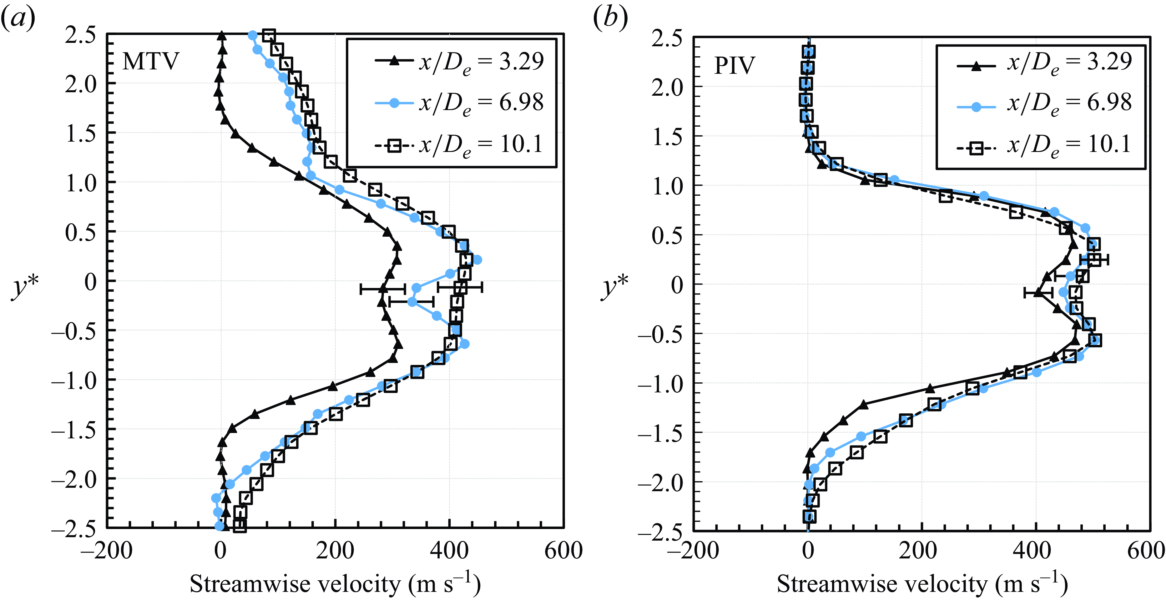
Figure 10. Streamwise mean velocity profile in the near-field zone for (a) MTV and (b) PIV.
Velocity profiles are overlaid in figure 11(a) to compare the velocity reduction near the jet exit. Initially, MTV velocities are faster, but after the Mach disk, the centreline velocity decreases by more than half, while PIV shows only a slight reduction. This suggests that in a rarefied environment, the discrete changes in fluid properties, such as pressure and density caused by the shockwave, lead to a rapid increase in the Stokes number. The particle relaxation time scale increases more relative to the increase in the fluid time scale, thus the particles are not able to suddenly reduce their velocity, which is the case shown by MTV. A direct comparison of post Mach disk velocity profiles is similarly overlaid in figure 11(b). As the streamwise mean velocity profile indicates, the jet gradually spreads radially downstream, showing a slight velocity increase. However, the PIV does not properly capture this.
The MTV data are featured in figure 12 to examine the evolution of the entire jet velocity profile in the near-field zone. The jet velocity has a single strong peak near the outlet before reaching the Mach disk, then substantially diminishes to form two peaks, and subsequently increases while the jet gradually spreads radially outward. The dual-peak pattern becomes most prominent at $x/D_{\textit {e}} = 6.98$
, likely due to the influence of the reflected shockwave in the surrounding area after the Mach disk. The centreline velocity continues to increase thereafter, and eventually, as the centreline and maximum velocities become similar, the dual-peak velocity profile gradually disappears.
$x/D_{\textit {e}} = 6.98$
, likely due to the influence of the reflected shockwave in the surrounding area after the Mach disk. The centreline velocity continues to increase thereafter, and eventually, as the centreline and maximum velocities become similar, the dual-peak velocity profile gradually disappears.
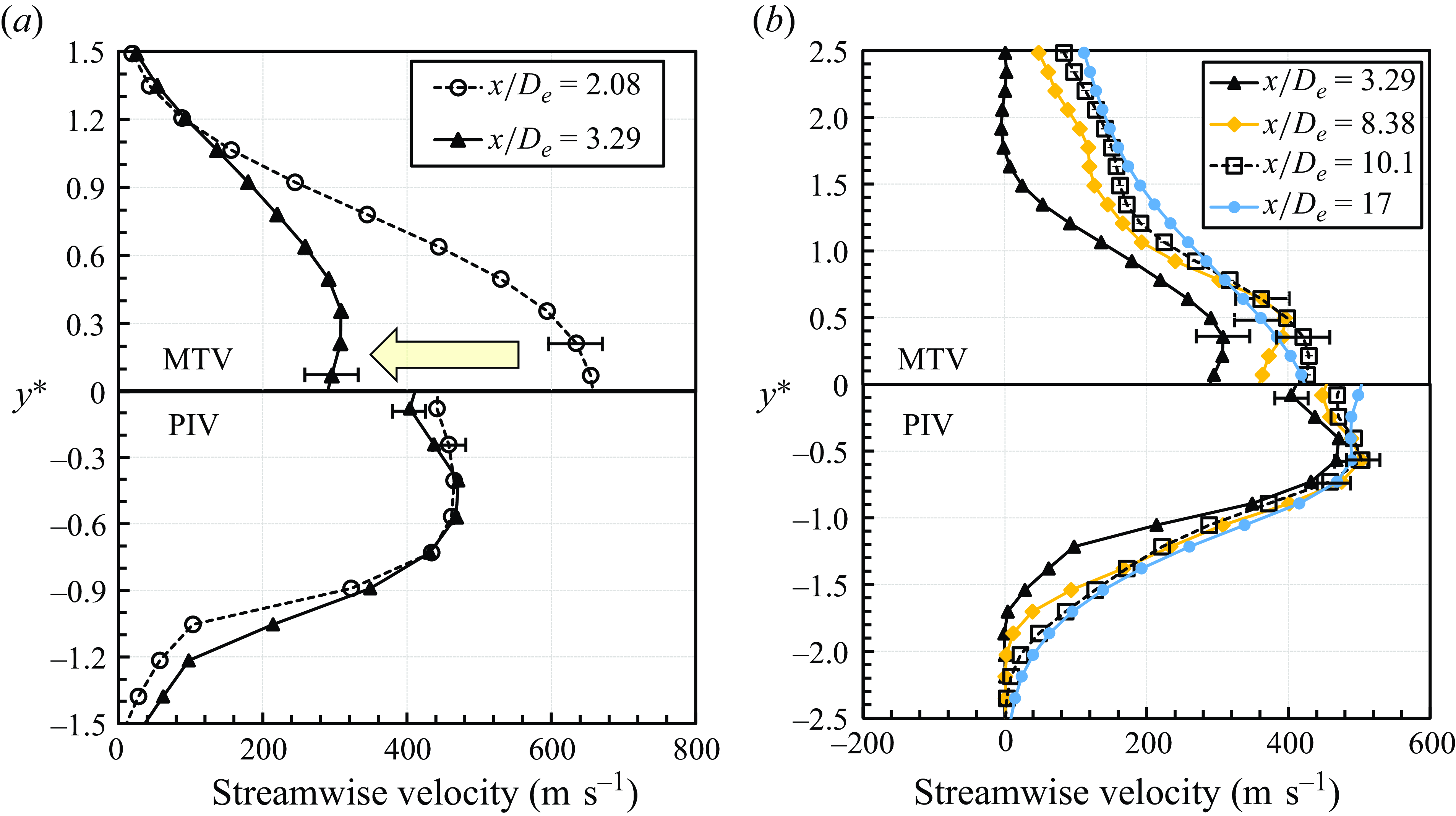
Figure 11. Streamwise mean velocity profiles (a) before and after the Mach disk and (b) comparisons after the Mach disk in the near-field zone.
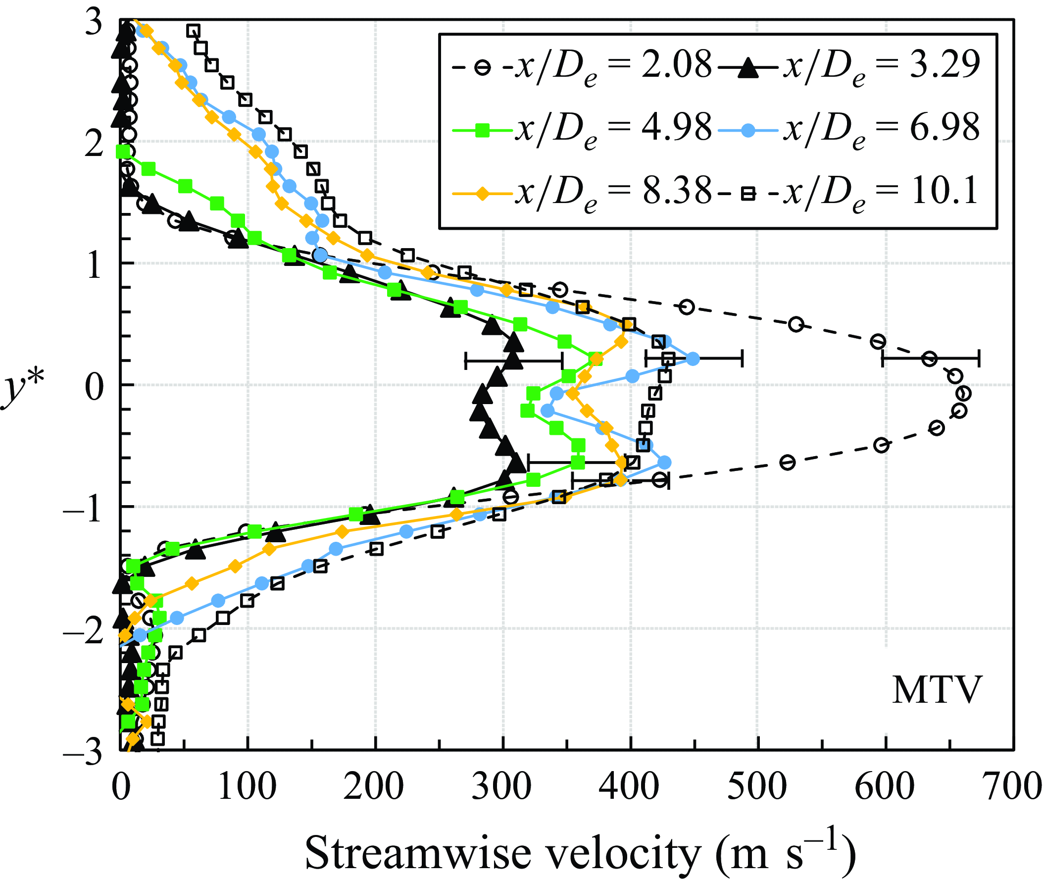
Figure 12. Evolution of the streamwise mean velocity profile in the near-field zone using MTV.
4.1.3. Far-field zone
The velocity distribution in the far-field zone was also illustrated in figure 9. It is noteworthy that both MTV and PIV showed converging centreline and maximum velocity distributions. The alignment of the distributions suggests that in the far-field zone, the absence of shockwave structures allows PIV to effectively follow the flow. Figure 13 demonstrates that the MTV and PIV streamwise mean velocity profiles are similar, adhering to a Gaussian profile, without the characteristic dual peaks observed in the near-field zone. This indicates that these measurement techniques are consistent with each other in capturing the flow in the far-field zone, and suggests that the jet exhibits self-similarity akin to a subsonic free jet.
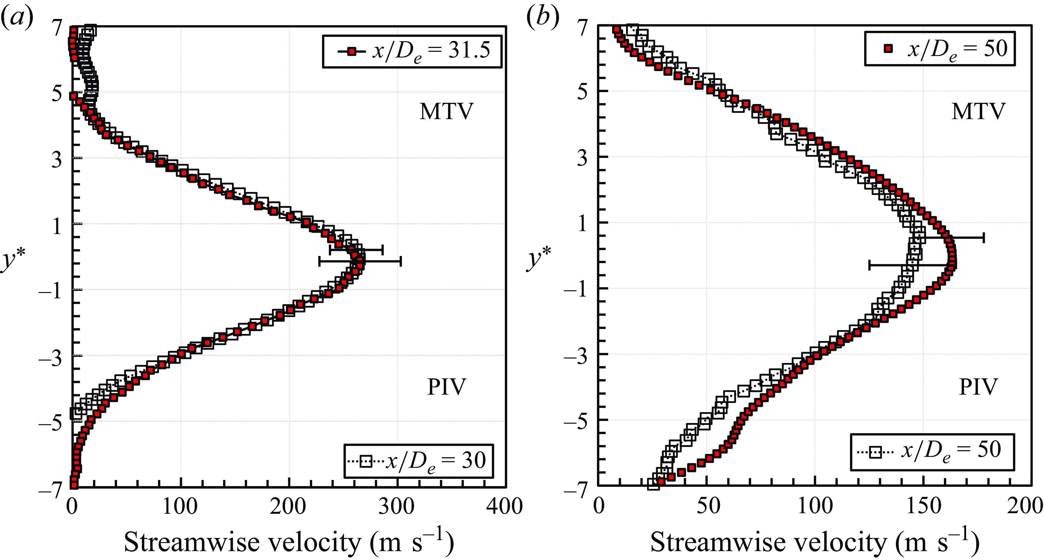
Figure 13. Streamwise mean velocity profile comparison between MTV and PIV at (a) $x/D_{\textit{e}}= 30$
and (b)
$x/D_{\textit{e}}= 30$
and (b) $x/D_{\textit{e}} = 50$
.
$x/D_{\textit{e}} = 50$
.
Indeed, as shown in figure 14, normalised streamwise mean velocity profiles at various streamwise locations collapse onto each other, confirming the jet’s self-similarity. This also allows for calculation of the jet spreading rate, as depicted in figure 15. The observed spreading rate of approximately 0.1 is consistent with that of a turbulent jet, implying that the jet in the far-field zone is turbulent.
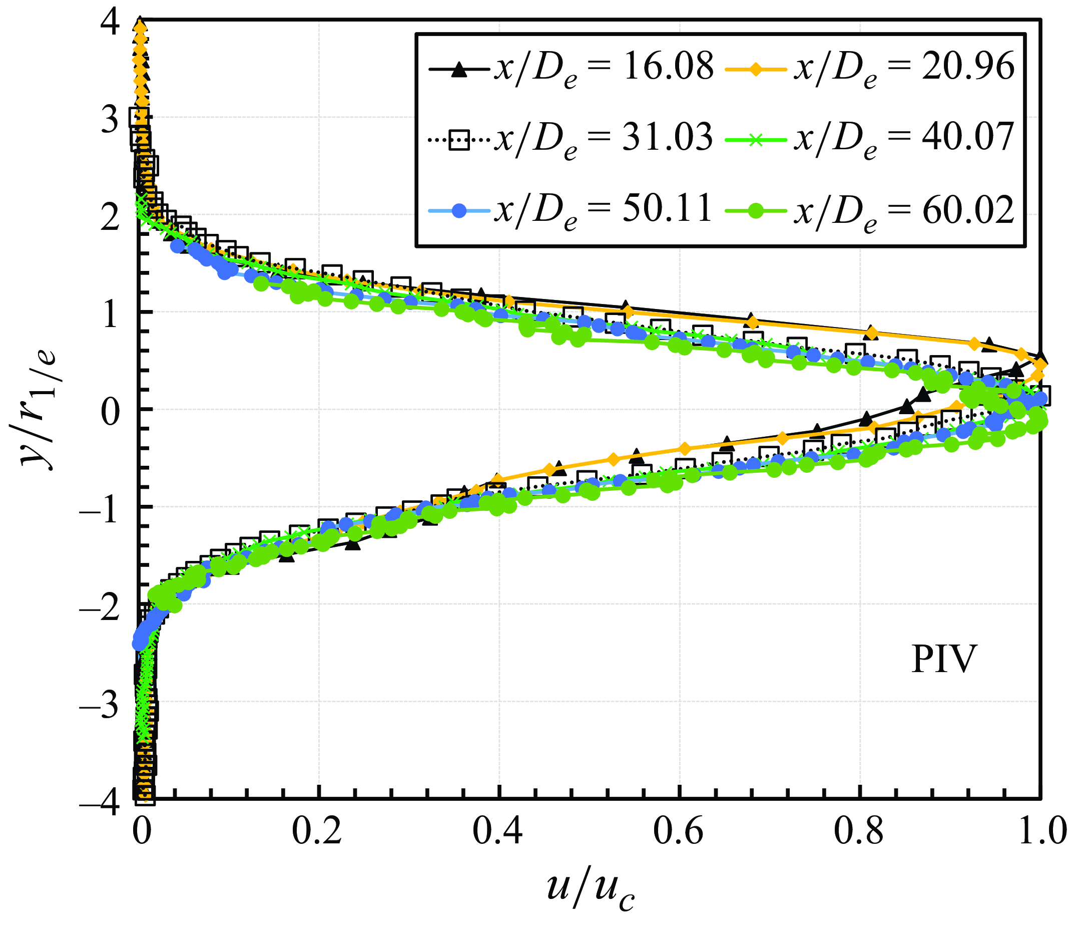
Figure 14. Streamwise mean velocity profiles (PIV) in the far-field zone normalised with centreline velocity ( $u_{\textit {c}}$
) and jet radius (
$u_{\textit {c}}$
) and jet radius ( $r_{\textrm {1/e}}$
) defined by the radial distance where the streamwise velocity decreases to
$r_{\textrm {1/e}}$
) defined by the radial distance where the streamwise velocity decreases to $1/e$
of the centreline maximum velocity.
$1/e$
of the centreline maximum velocity.
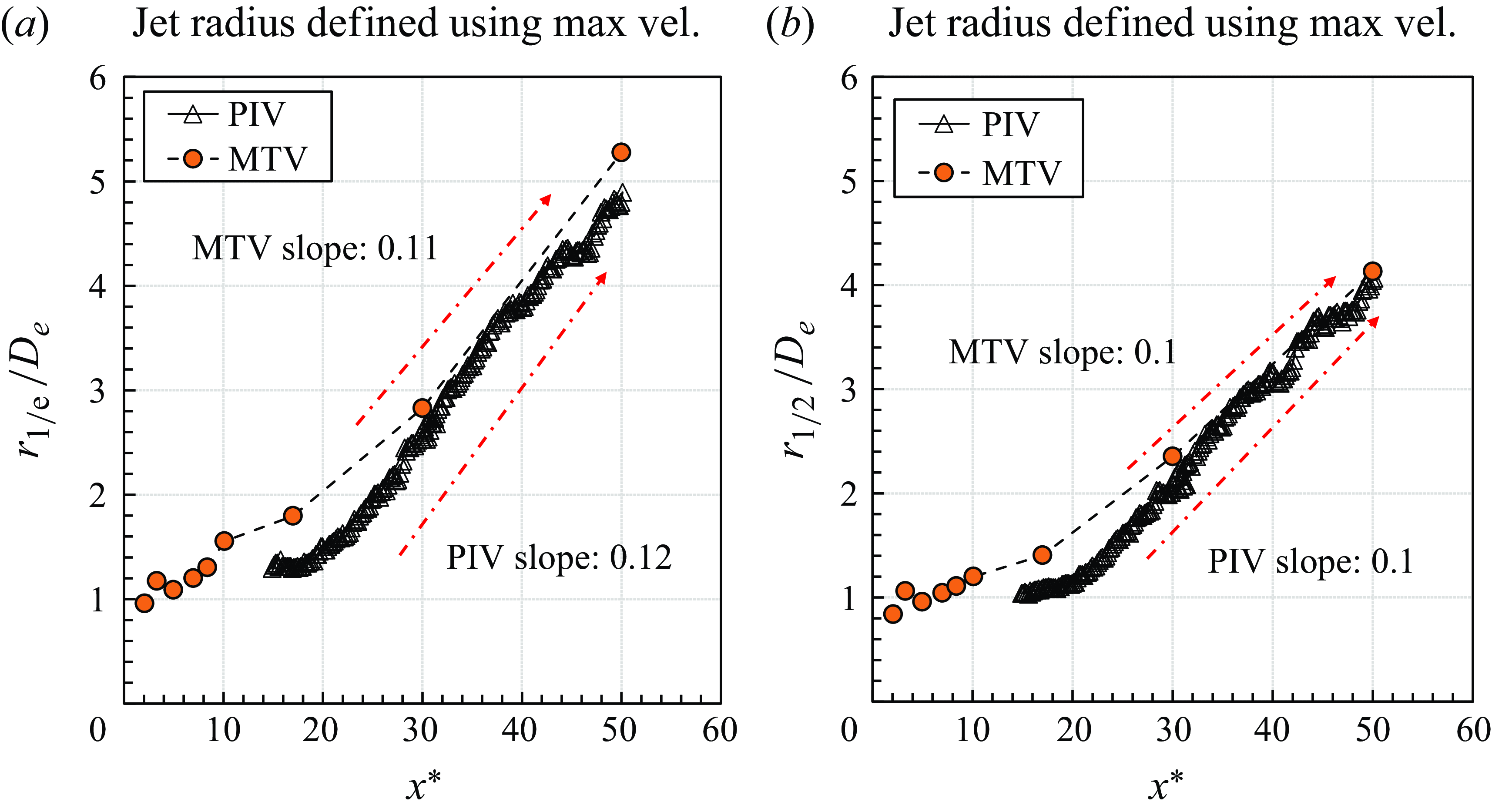
Figure 15. Normalised jet radius defined by the radial distance where the streamwise velocity decreases to (a) $1/e$
and (b) half of the maximum velocity.
$1/e$
and (b) half of the maximum velocity.
As the jet satisfies self-similarity, modelling of the centreline velocity in the far-field zone can proceed in a manner similar to that of a subsonic jet. However, as noted by Birch, Hughes & Swaffield (Reference Birch, Hughes and Swaffield1987), the decay constant varies with the NPR, different to typical incompressible turbulent jets. The evolution of the centreline velocity, incorporating the NPR, is displayed in figure 16. The current slope 0.193 aligns with studies conducted under atmospheric pressure conditions (Ball, Fellouah & Pollard Reference Ball, Fellouah and Pollard2012). This relationship can be expressed as
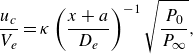 \begin{equation} \frac {u_{\textit {c}}}{V_{\textit {e}}}=\kappa \left(\frac {x+a}{D_{\textit {e}}}\right)^{-1}\sqrt {\frac {P_{0}}{P_{\infty }}}, \end{equation}
where $u_{\textit {c}}$
is the centreline velocity,
$u_{\textit {c}}$
is the centreline velocity, $V_{\textit {e}}$
is the outlet velocity magnitude,
$V_{\textit {e}}$
is the outlet velocity magnitude, $\kappa$
is the decay constant,
$\kappa$
is the decay constant, $x$
is the streamwise position, and
$x$
is the streamwise position, and $a$
is the momentum virtual origin. From the linearised form of the data in figure 16, the value of
$a$
is the momentum virtual origin. From the linearised form of the data in figure 16, the value of $1/\kappa$
was determined to be approximately 0.193, corresponding to a decay constant
$1/\kappa$
was determined to be approximately 0.193, corresponding to a decay constant $\kappa \sim 5.18$
. To determine the momentum virtual origin
$\kappa \sim 5.18$
. To determine the momentum virtual origin $a$
, a least mean squares fitting approach was employed to maximise the
$a$
, a least mean squares fitting approach was employed to maximise the $\mathrm{R^2}$
value (0.99) of the fit. This yielded
$\mathrm{R^2}$
value (0.99) of the fit. This yielded $a=13.66D_{{e}}$
, ensuring the highest accuracy in representing the data.
$a=13.66D_{{e}}$
, ensuring the highest accuracy in representing the data.
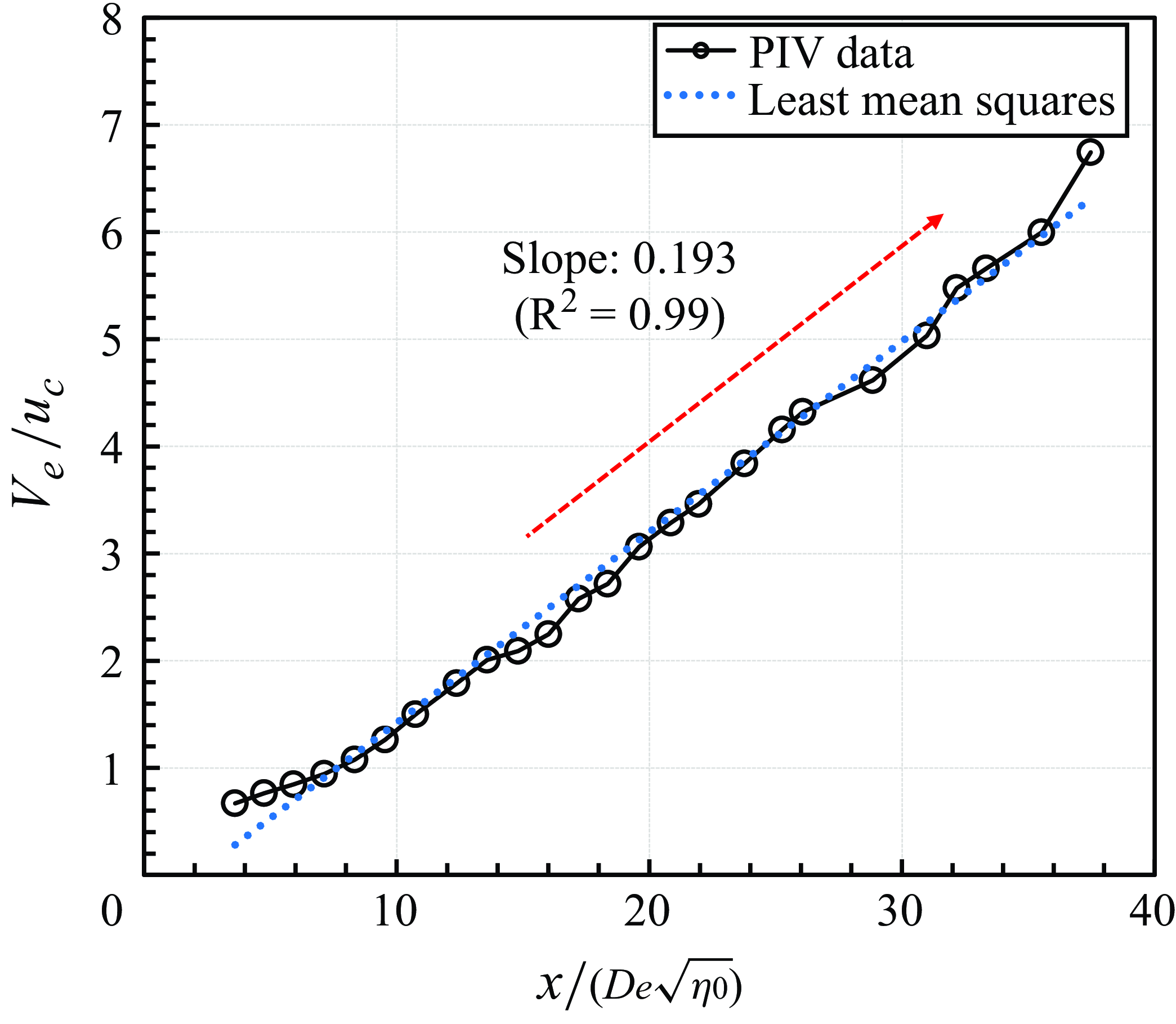
Figure 16. Evolution of inverse normalised centreline streamwise mean velocity.
The PIV data were used to calculate turbulent statistics in the far-field zone. Figure 17 presents both centreline streamwise and spanwise turbulence intensities that increase moving downstream, peaking at approximately $x/D_{{e}}=60{-}70$
before decreasing. This peak can be attributed to the delayed convergence of turbulent energy in the fully developed region. While the jet achieves self-similarity in mean velocity earlier, turbulent characteristics continue to evolve downstream. Statistics of streamwise (u′
) and spanwise (v′
) velocity fluctuations converge later compared to those of the mean velocity, causing turbulence intensity to peak at
$x/D_{{e}}=60{-}70$
before decreasing. This peak can be attributed to the delayed convergence of turbulent energy in the fully developed region. While the jet achieves self-similarity in mean velocity earlier, turbulent characteristics continue to evolve downstream. Statistics of streamwise (u′
) and spanwise (v′
) velocity fluctuations converge later compared to those of the mean velocity, causing turbulence intensity to peak at $x/D_{{e}}=60{-}70$
before decreasing as the flow becomes fully turbulent. Streamwise turbulence intensity converges at approximately 28 %, while spanwise turbulence intensity seems to converge at approximately 20 %, aligning with results from previous studies (Wygnanski & Fiedler Reference Wygnanski and Fiedler1969; Panchapakesan & Lumley Reference Panchapakesan and Lumley1993; Xu & Antonia Reference Xu and Antonia2002; Burattini, Antonia & Danaila Reference Burattini, Antonia and Danaila2005; Quinn Reference Quinn2006). These studies also demonstrated that turbulence intensity reaches a steady value in the fully developed region of turbulent jets, reflecting self-similarity after sufficient mixing. The agreement with these studies further supports the classification of the far-field jet as being turbulent.
$x/D_{{e}}=60{-}70$
before decreasing as the flow becomes fully turbulent. Streamwise turbulence intensity converges at approximately 28 %, while spanwise turbulence intensity seems to converge at approximately 20 %, aligning with results from previous studies (Wygnanski & Fiedler Reference Wygnanski and Fiedler1969; Panchapakesan & Lumley Reference Panchapakesan and Lumley1993; Xu & Antonia Reference Xu and Antonia2002; Burattini, Antonia & Danaila Reference Burattini, Antonia and Danaila2005; Quinn Reference Quinn2006). These studies also demonstrated that turbulence intensity reaches a steady value in the fully developed region of turbulent jets, reflecting self-similarity after sufficient mixing. The agreement with these studies further supports the classification of the far-field jet as being turbulent.
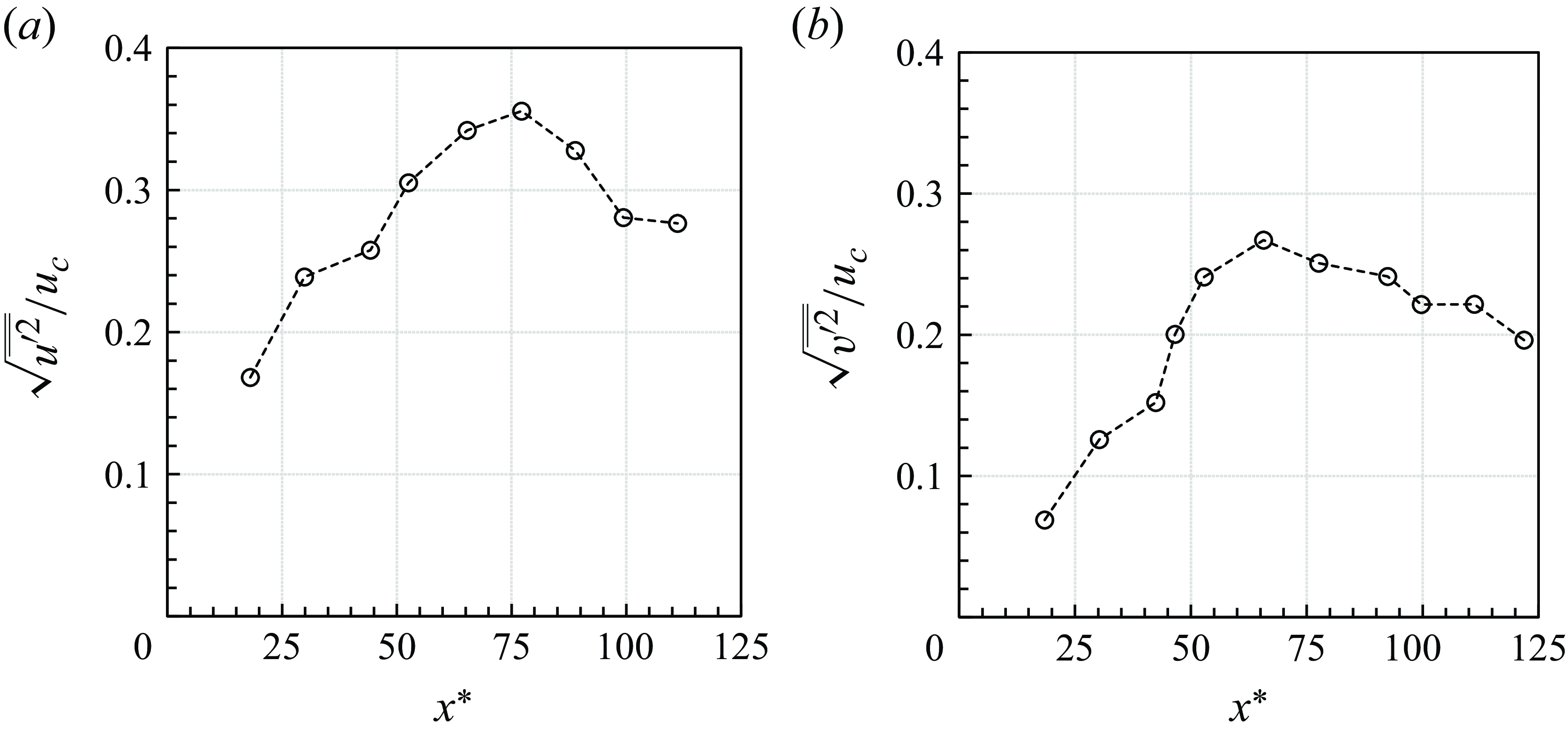
Figure 17. Evolution of centreline (a) streamwise and (b) spanwise turbulence intensity.
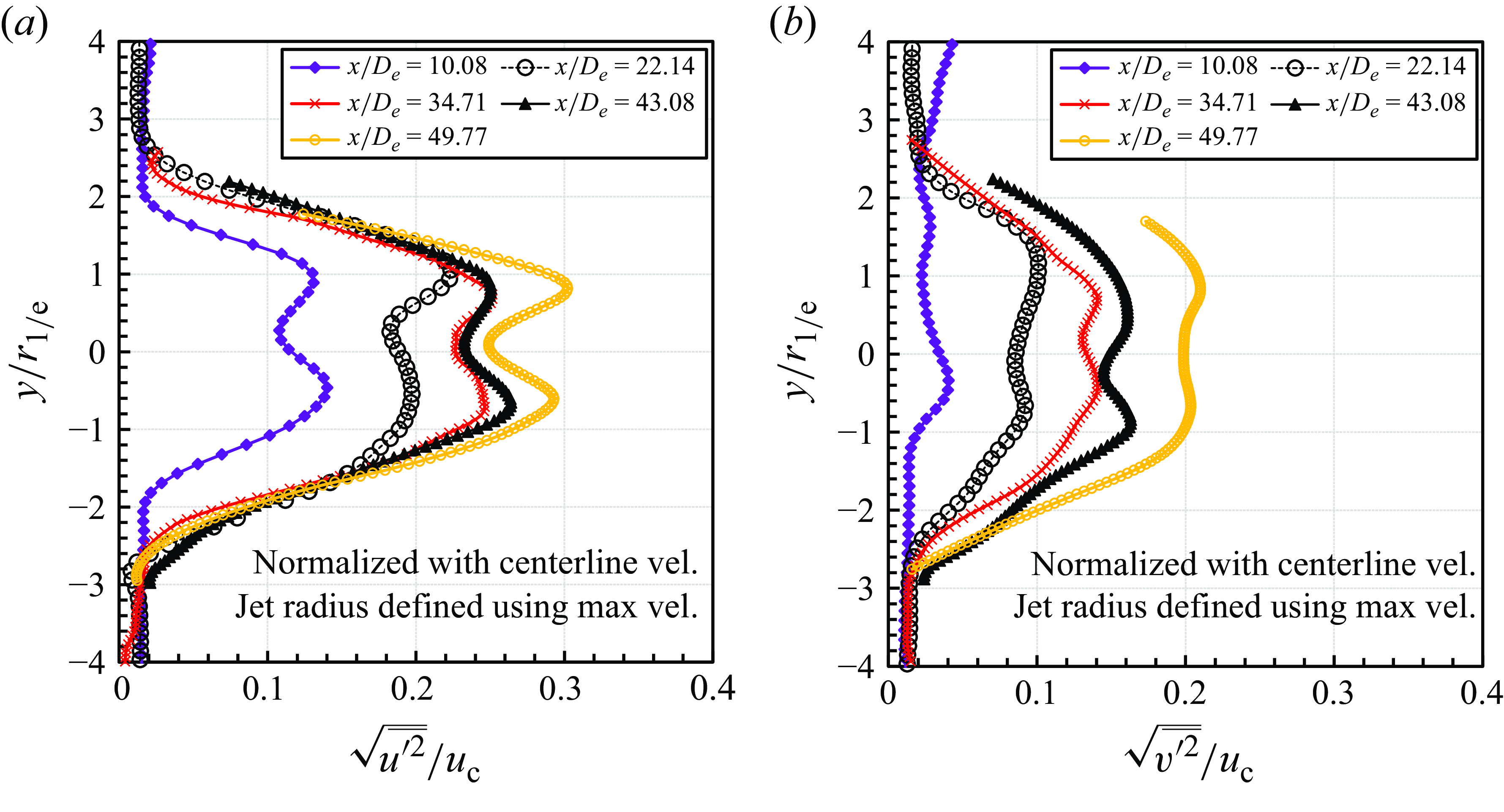
Figure 18. Turbulence intensity profiles for various downstream positions in the far-field zone.
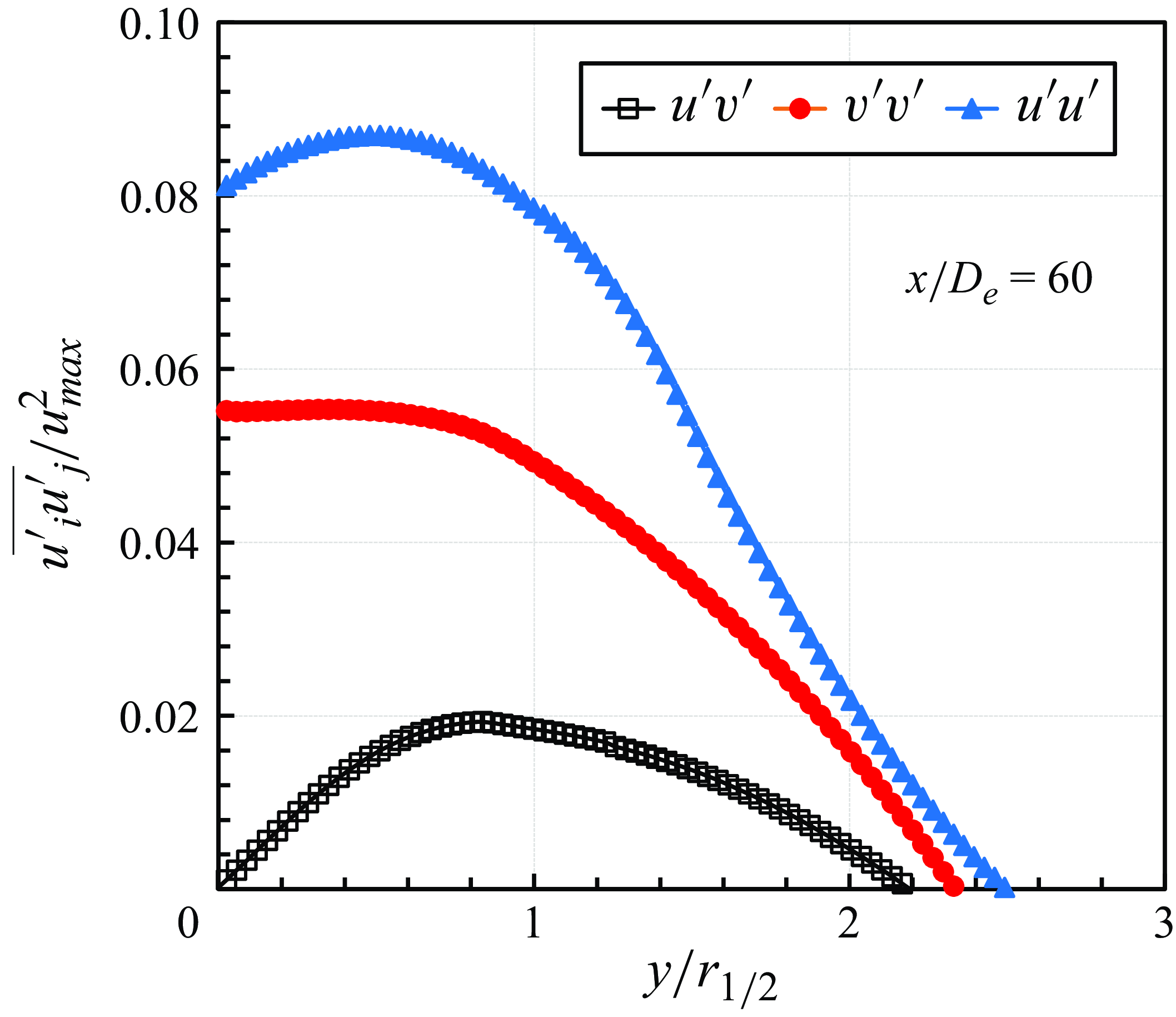
Figure 19. Reynolds stress profiles at $x/D_{{e}}= 60$
in the far-field zone.
$x/D_{{e}}= 60$
in the far-field zone.
Normalised turbulence intensity profiles are plotted in figure 18. The streamwise turbulence intensity displays more distinctive dual-peak patterns compared to the spanwise case. Additionally, the Reynolds shear and normal stress profiles are presented in figure 19, demonstrating close similarity to Reynolds stresses of atmospheric turbulent free jets observed in previous experimental results (Hussein, Capp & George Reference Hussein, Capp and George1994). This further indicates that the turbulent viscosity, which is determined by the gradient of the streamwise mean velocity and Reynolds shear stress, also follows a similar pattern. Furthermore, proper orthogonal decomposition (POD) analysis was conducted to analyse the coherent structures of turbulence in the far-field zone. The detailed methodology and results of the POD analysis have been included in Appendix D for further reference. Overall, the results reveal that turbulent jet behaviour remains similar with atmospheric conditions. Even as the flow becomes more rarefied and stable, its characteristics are preserved under reduced pressure.
4.2. Extremely under-expanded supersonic free jet (laminar flow regime)
4.2.1. Shockwave structure
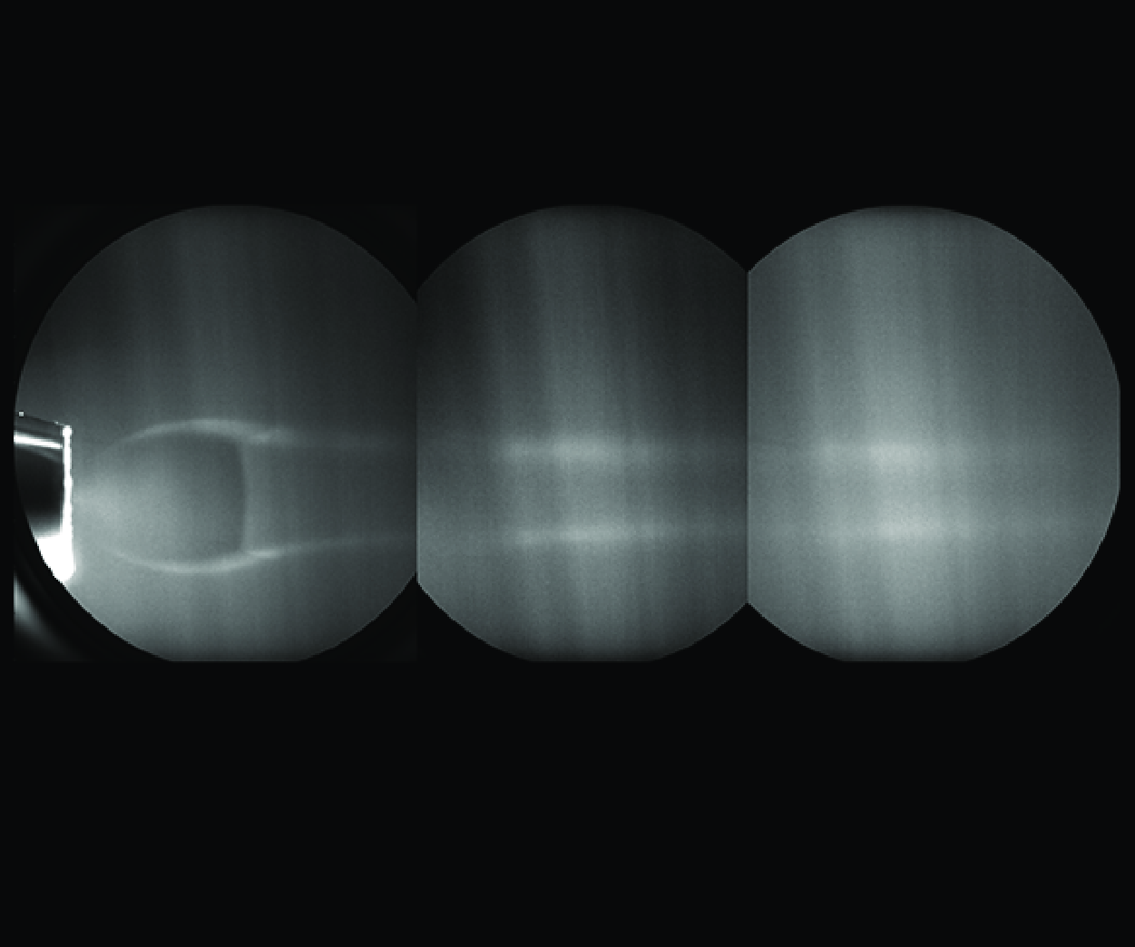
The LIF was performed to visualise the structure of the supersonic free jet under the conditions listed in table 1. The LIF image shown in figure 20 was obtained by ensemble averaging 100 individual images using an integration technique. As clearly depicted in figure 20(a), the presence of a barrel shockwave and a central Mach disk can be identified. Beyond the Mach disk, no additional shockwave structures are observed, and a long annular shear layer persists in the far-field zone. The Mach disk exhibits slight curvature due to the high pressure difference. Studies examining shockwave structures of a supersonic free jet in a rarefied environment with NPR exceeding 100 are scarce, but comparisons with a limited number of studies reveal a very similar structure (Volchkov et al. Reference Volchkov, Ivanov, Kislyakov, Rebrov, Sukhnev and Sharafutdinov1973; Belan et al. Reference Belan, De Ponte and Tordella2008, Reference Belan, de Ponte, Tordella, Massaglia, Mignone, Bodenschatz and Ferrari2011; Shurtz & West Reference Shurtz and West2022). The key features at each location are indicated schematically in figure 20(b). The annular shear layer within the inner and outer shear layers fundamentally acts as a mixing zone. The mixing stems from the dual-peak velocity profile created by the Mach disk, with shear arising between the velocity peak and both the slower-moving jet interior (inner region) and ambient fluid (outer region).
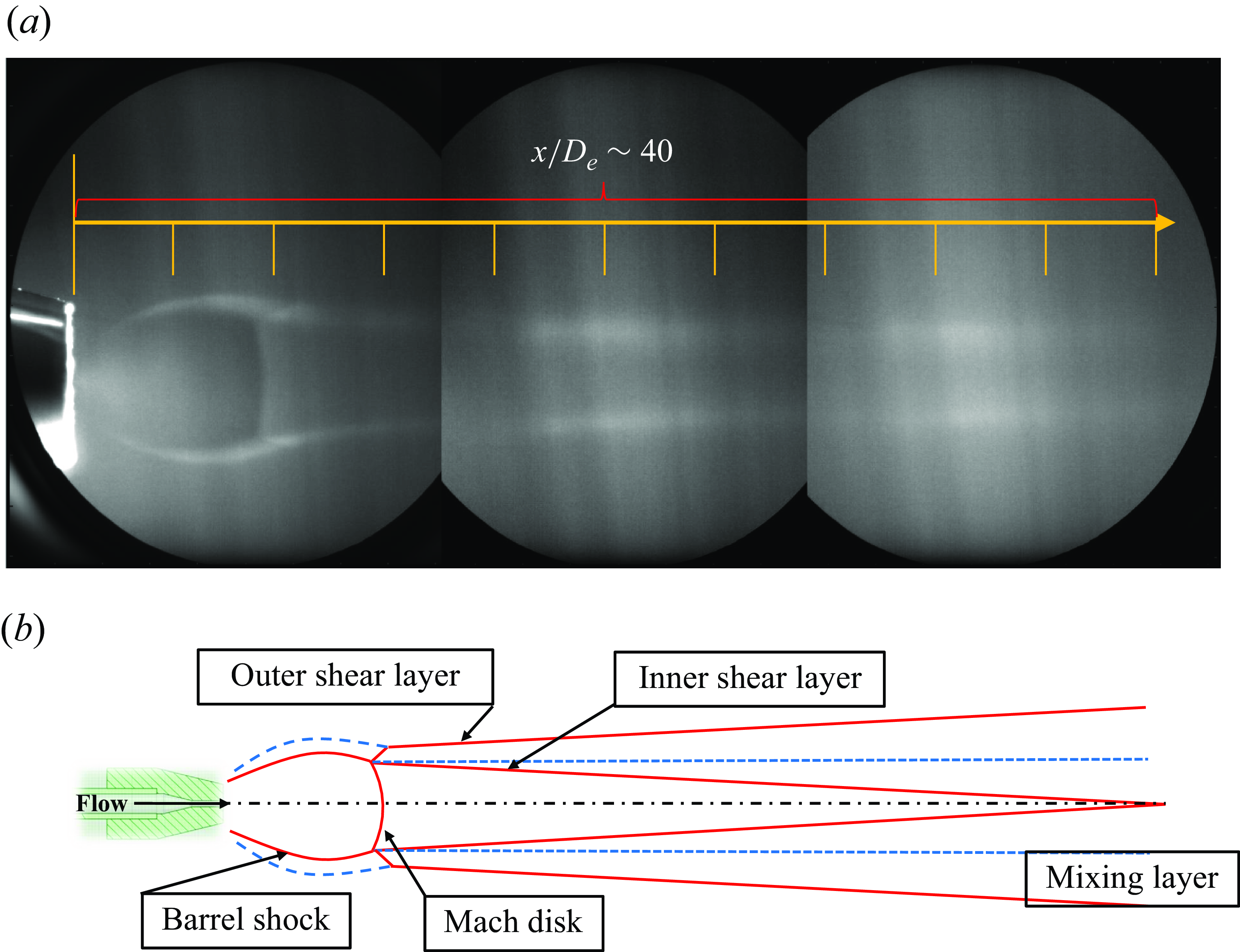
Figure 20. Combined LIF field of view for extremely under-expanded supersonic free jet: (a) single-barrel shockwave with long annular shear layer, and (b) schematic of flow structure.
4.2.2. Near-field zone
Similar to a highly under-expanded supersonic free jet, to analyse the overall characteristics of the jet considering the shockwave structure, we assessed the centreline and maximum velocities. In the case of an extremely under-expanded supersonic free jet, as illustrated in figure 21, the initially discharged flow undergoes a sharp velocity increase due to free expansion. The differences between MTV and PIV are even more pronounced than for the previous highly under-expanded supersonic free jet. While MTV appears to track this sudden increase accurately, PIV registers only a slight velocity increase. As the gas exits the nozzle, the tracer particles are unable to respond to the flow field changes, due to the decreased surrounding density following the expansion. After the initial spike in velocity, a subsequent sharp decrease occurs due to the Mach disk at $x^* \approx 8$
. Both MTV and PIV record a velocity decrease, but the reduction in PIV is significantly less pronounced compared to MTV. Mach disks increase the pressure, which then expands to match downstream conditions, resulting in an increasing velocity. The MTV captures this velocity increase due to the favourable pressure gradient. In contrast, PIV shows a prolonged decrease as the tracer particles’ inertia exceeds the pressure gradient, unlike in the 10 torr case. After the jet pressure equalises with the ambient pressure, the jet reaches the fully developed region where the centreline and maximum velocities converge, as seen from both MTV and PIV results.
$x^* \approx 8$
. Both MTV and PIV record a velocity decrease, but the reduction in PIV is significantly less pronounced compared to MTV. Mach disks increase the pressure, which then expands to match downstream conditions, resulting in an increasing velocity. The MTV captures this velocity increase due to the favourable pressure gradient. In contrast, PIV shows a prolonged decrease as the tracer particles’ inertia exceeds the pressure gradient, unlike in the 10 torr case. After the jet pressure equalises with the ambient pressure, the jet reaches the fully developed region where the centreline and maximum velocities converge, as seen from both MTV and PIV results.
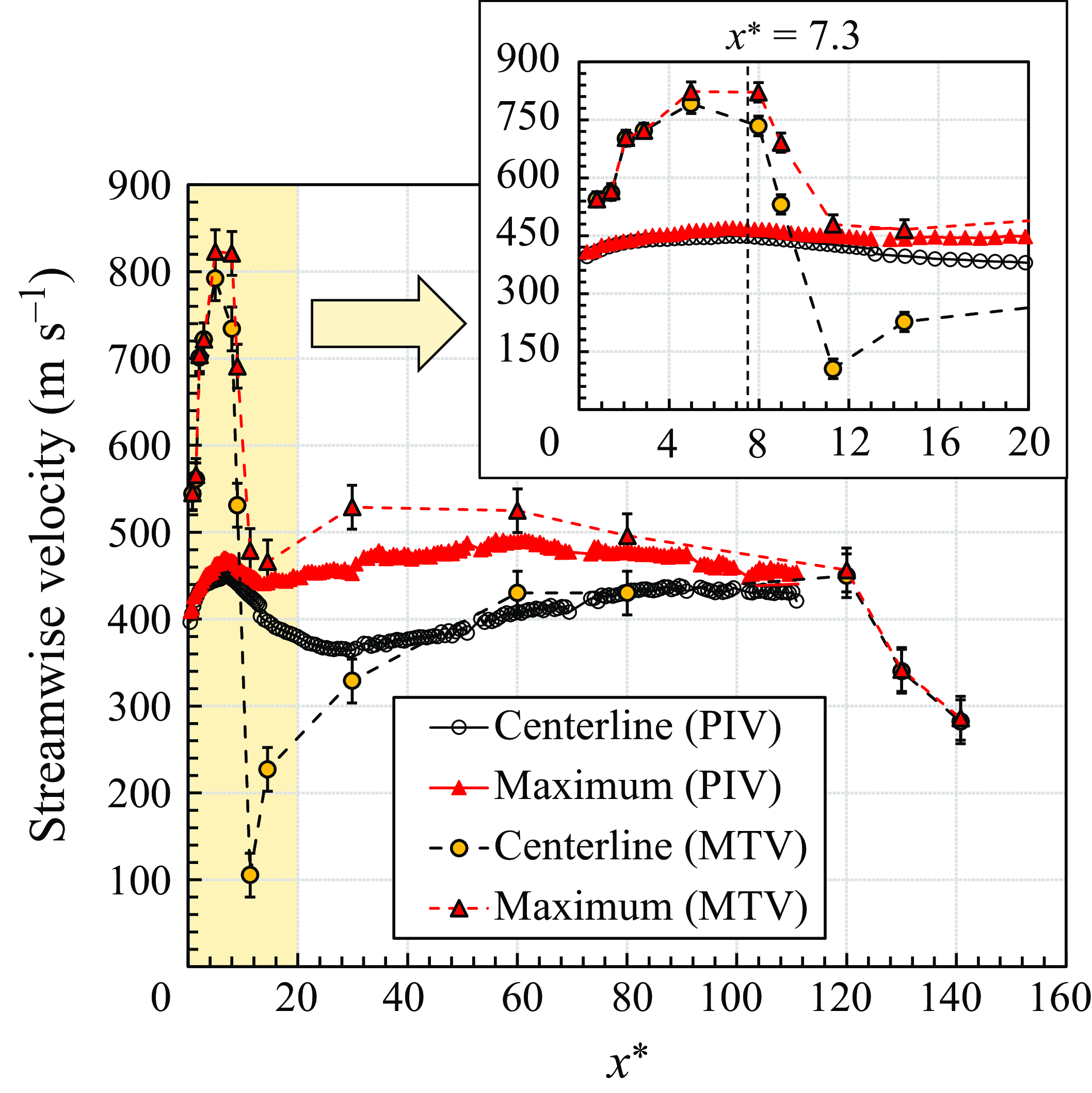
Figure 21. Evolution of centreline and maximum streamwise mean velocities for PIV and MTV.
Given the notable difference between MTV and PIV results in the near-field zone, a comparison with theoretical values is warranted. The theoretical Mach disk position and size were calculated using the following empirical equations, derived for conditions of ambient pressure higher than atmospheric pressure (Lewis, Clarke & Carlson Reference Lewis, Clarke and Carlson1964; Crist, Glass & Sherman Reference Crist, Glass and Sherman1966; Jiang et al. Reference Jiang, Han, Hu, Gao and Lee2022):
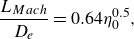 \begin{equation} \frac {L_{{Mach}}}{D_{\textit {e}}} =0.64\eta _0^{0.5}, \end{equation}
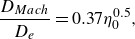 \begin{equation} \frac {D_{{Mach}}}{D_{\textit {e}}} =0.37\eta _0^{0.5}, \end{equation}
where $L_{{Mach}}$
and
$L_{{Mach}}$
and $D_{{Mach}}$
are the position and diameter of the Mach disk, respectively. The normalised positions of the Mach disk calculated using the equations are 7.3 for its normalised location, and 3.2 for its normalised diameter. We also determined the position of the Mach disk from the experimental data. Both the MTV centreline and maximum velocity results show a sharp decrease after normalised position 7.98, thus this was deemed to be the location of the Mach disk. This closely matches the Mach disk position observed in LIF measurements, with slight discrepancies attributed to the MTV spatial resolution limits. The results also align well with established empirical equations.
$D_{{Mach}}$
are the position and diameter of the Mach disk, respectively. The normalised positions of the Mach disk calculated using the equations are 7.3 for its normalised location, and 3.2 for its normalised diameter. We also determined the position of the Mach disk from the experimental data. Both the MTV centreline and maximum velocity results show a sharp decrease after normalised position 7.98, thus this was deemed to be the location of the Mach disk. This closely matches the Mach disk position observed in LIF measurements, with slight discrepancies attributed to the MTV spatial resolution limits. The results also align well with established empirical equations.
Next, we compare the flow properties at the zone of silence. Functional dependence of the Mach number $M(x)$
on downstream distance
$M(x)$
on downstream distance $x$
can be determined using the following equation (Morse Reference Morse1996) for a jet exiting from a sonic nozzle:
$x$
can be determined using the following equation (Morse Reference Morse1996) for a jet exiting from a sonic nozzle:
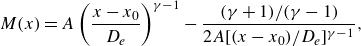 \begin{equation} M(x)=A\left (\frac {x-x_0}{D_{\textit {e}}}\right )^{\gamma -1}-\frac {(\gamma +1)/(\gamma -1)}{2A[(x-x_0)/D_{\textit {e}}]^{\gamma -1}}, \end{equation}
where $\gamma$
is the specific heat ratio, and
$\gamma$
is the specific heat ratio, and $x_0/D_{{e}}$
and
$x_0/D_{{e}}$
and $A$
depend on
$A$
depend on $\gamma$
. The parameter
$\gamma$
. The parameter $A$
is a coefficient introduced by Morse (Reference Morse1996) that depends on the nozzle geometry and characterises the specific expansion properties of the jet. For a supersonic free
$A$
is a coefficient introduced by Morse (Reference Morse1996) that depends on the nozzle geometry and characterises the specific expansion properties of the jet. For a supersonic free $\mathrm{N_{2}}$
jet,
$\mathrm{N_{2}}$
jet, $\gamma$
is 1.3, resulting in
$\gamma$
is 1.3, resulting in $x_0/D_{{e}}= 0.7$
and
$x_0/D_{{e}}= 0.7$
and $A=3$
. It is important to note that (4.4) is not influenced by the NPR or the Reynolds number. Instead, it was derived analytically based on the free expansion of fluid from a sonic nozzle, and describes the centreline Mach number development within the zone of silence, a region of adiabatic, non-viscous expansion. As discussed in Rebrov (Reference Rebrov2001), this equation assumes that the zone of silence remains in the continuum regime, surrounded by the barrel shock up to the Mach disk, where isentropic relations apply. If the flow at the nozzle outlet were not in the continuum regime, then (4.4) would no longer be valid. However, in our study, the flow at the nozzle outlet meets this criterion, allowing us to apply this model.
$A=3$
. It is important to note that (4.4) is not influenced by the NPR or the Reynolds number. Instead, it was derived analytically based on the free expansion of fluid from a sonic nozzle, and describes the centreline Mach number development within the zone of silence, a region of adiabatic, non-viscous expansion. As discussed in Rebrov (Reference Rebrov2001), this equation assumes that the zone of silence remains in the continuum regime, surrounded by the barrel shock up to the Mach disk, where isentropic relations apply. If the flow at the nozzle outlet were not in the continuum regime, then (4.4) would no longer be valid. However, in our study, the flow at the nozzle outlet meets this criterion, allowing us to apply this model.
Using the aforementioned equation and isentropic relation, absolute streamwise velocity can be determined and compared with experimental results. Figure 22 presents comparisons among theoretical, MTV and PIV results for centreline streamwise velocity. The zone of silence up to the Mach disk is a free expansion zone and should exhibit the same velocity profile for both ambient pressures. As is evident from the plot, PIV data do not align with theoretical values, regardless of the pressure condition (1 torr or 10 torr). Additionally, theoretical streamwise velocity before and after the Mach disk was calculated using Mach numbers derived from the calorically perfect normal shock relation. From these calculations, the theoretical velocity was estimated to be approximately 126 m s−1. This value corresponds to the lowest streamwise velocity observed in the post-Mach-disk region, and aligns closely with the MTV measurement 105 m s−1, considering experimental uncertainties as depicted in figure 21.
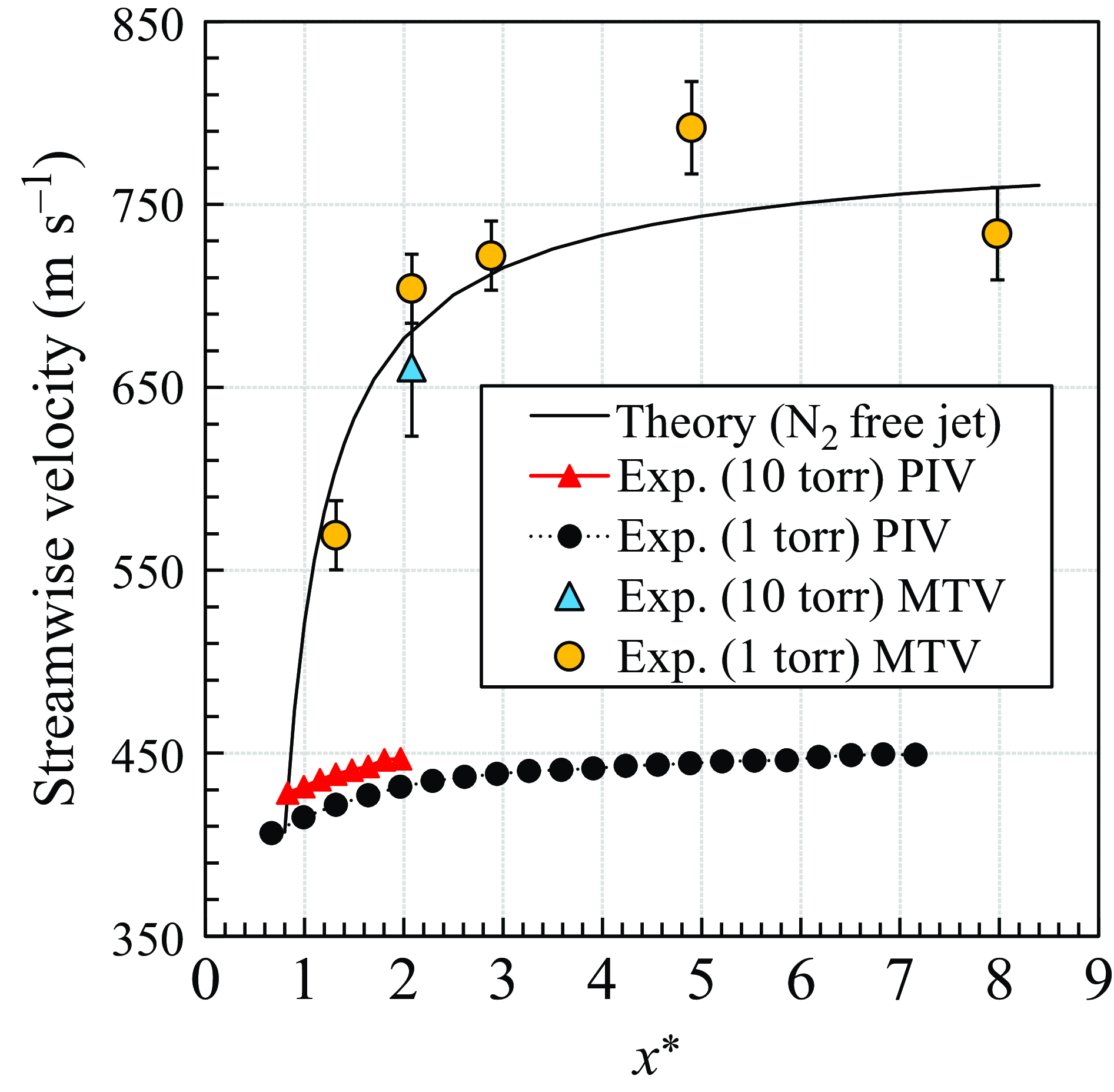
Figure 22. Comparison between experimental centreline streamwise velocity and theory.
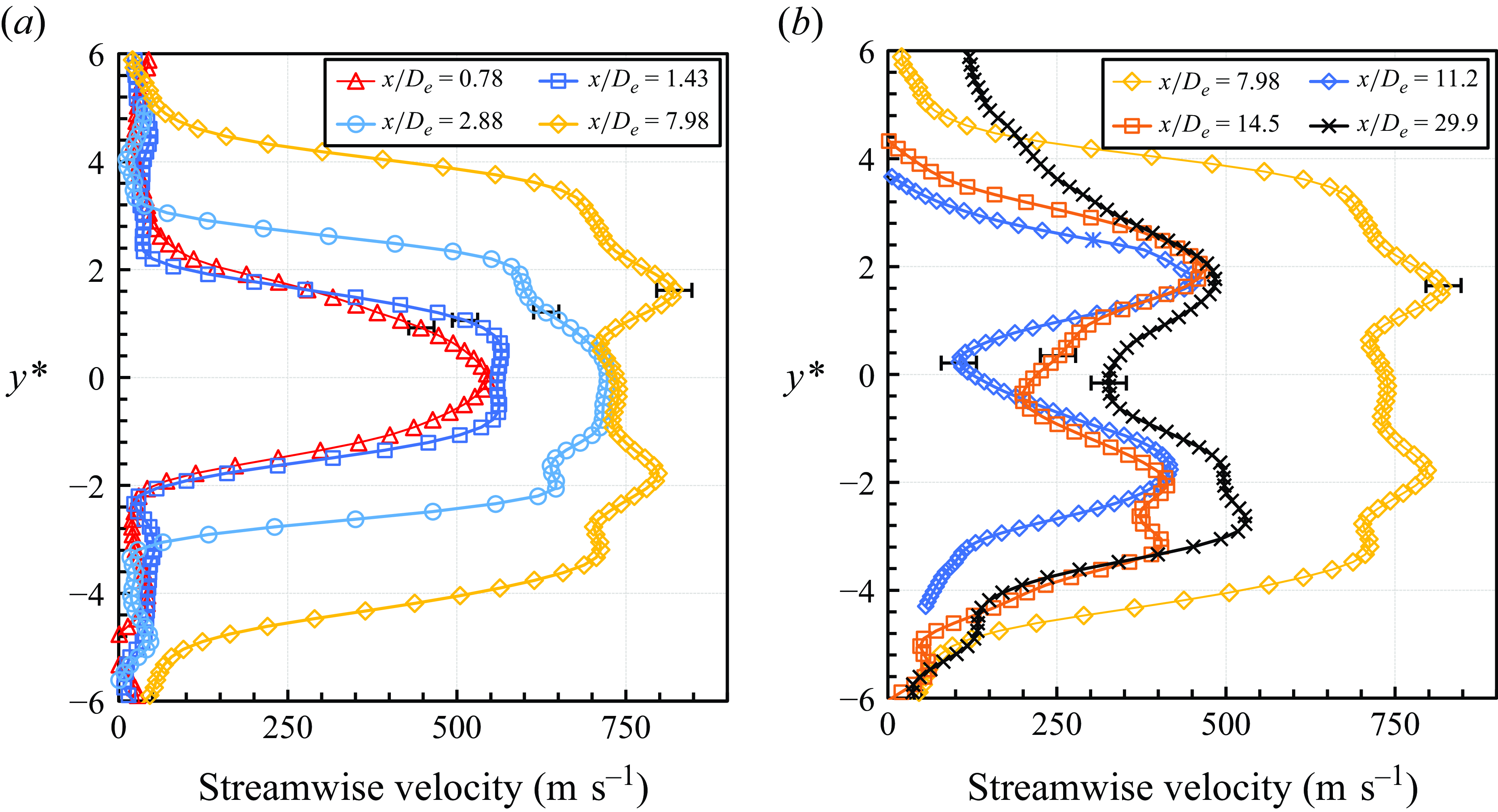
Figure 23. Streamwise mean velocity profiles (a) before and (b) after the Mach disk.
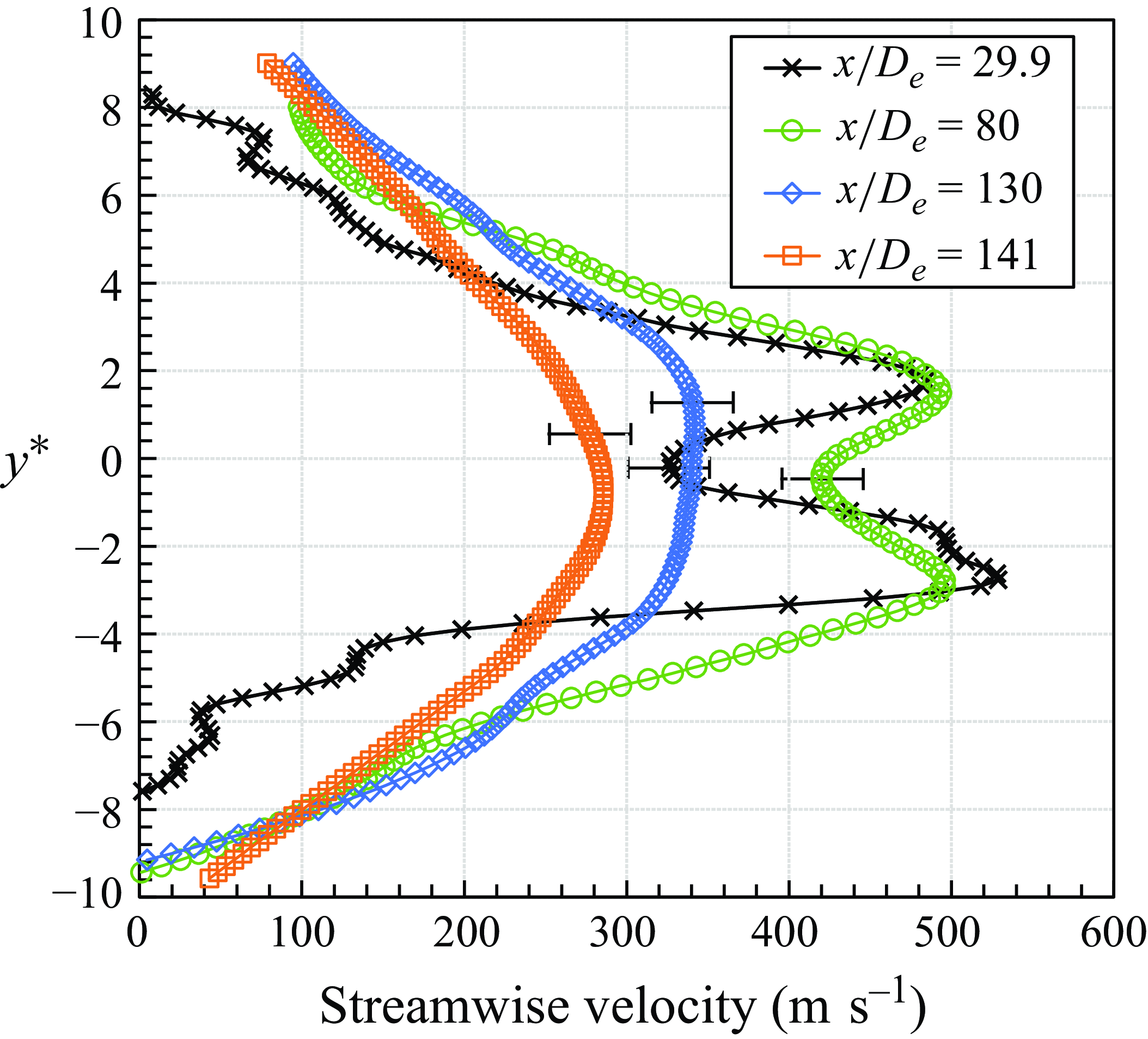
Figure 24. Evolution of streamwise mean velocity profile in the potential core region and far-field zone.
To observe the evolution of the streamwise mean profile in the near-field zone, velocity profiles at various streamwise positions before and after the Mach disk are presented for the MTV results in figure 23. Figure 23(a) illustrates that the velocity consistently increases after the jet is discharged from the nozzle due to flow expansion. In figure 23(b), the velocity profile is deformed due to interactions with the barrel shock, and decreases (as expected) after the Mach disk, forming a distinct double-peak profile. As the jet progresses downstream, velocities gradually increase, primarily due to favourable pressure gradients. This velocity increment phenomenon for a one-barrel shock is similarly observed in supersonic free jets at atmospheric pressure (Jerónimo et al. Reference Jerónimo, Riethmuller and Chazot2002; Xiao et al. Reference Xiao, Fond, Beyrau, T’Joen, Henkes, Veenstra and van Wachem2019).
In a supersonic free jet, the potential core extends to the point where the annular shear layers merge at the jet centreline (Franquet et al. Reference Franquet, Perrier, Gibout and Bruel2015). In our study, this zone is identified as the point where the centreline and maximum velocities become equal to each other, as illustrated in figure 21. The primary focus within this zone is the development of the mixing layer, particularly how the inner and outer shear layers evolve due to the influence of the Mach disk. Unlike the zone of silence, this region is significantly affected by viscosity, making the application of isentropic relations challenging.
Further analysis was conducted by examining the streamwise mean velocity profiles obtained from MTV at key locations after the Mach disk at $x/D_{\textit {e}}= 7.98$
, as presented in figure 24. Following the Mach disk, the velocity profile exhibits a large dual peak with a substantial velocity gradient. As the flow progresses downstream, both inner and outer shear layers develop concurrently. Eventually, these dual peaks merge into a single peak as the flow transitions into the far-field zone in figure 21. Subsequently, as the momentum diffuses outwards, the centreline velocity begins to decay, and the jet spreads radially outward.
$x/D_{\textit {e}}= 7.98$
, as presented in figure 24. Following the Mach disk, the velocity profile exhibits a large dual peak with a substantial velocity gradient. As the flow progresses downstream, both inner and outer shear layers develop concurrently. Eventually, these dual peaks merge into a single peak as the flow transitions into the far-field zone in figure 21. Subsequently, as the momentum diffuses outwards, the centreline velocity begins to decay, and the jet spreads radially outward.
4.2.3. Far-field zone
The velocity distribution in the far-field zone was also illustrated in figure 21. A dramatic velocity decrease is observed. This phenomenon is attributed to two factors. First, this region marks the transition from the potential core to the fully developed region. In the potential core, the centreline velocity remains high due to favourable pressure gradients and momentum transfer from surrounding high-velocity regions. In the fully developed region, the velocity profile evolves into a Gaussian distribution, leading to significant momentum transfer from the centreline to the surroundings, and a more rapid velocity decay. Second, the velocity decay in the fully developed region is proportional to the inverse streamwise distance ( $1/x^*$
), consistent with the behaviour of free jets observed in prior studies, such as Birch et al. (Reference Birch, Hughes and Swaffield1987).
$1/x^*$
), consistent with the behaviour of free jets observed in prior studies, such as Birch et al. (Reference Birch, Hughes and Swaffield1987).
In the far-field zone, the jet transitions to a Gaussian-shaped fully developed velocity profile. Velocity profiles normalised by the jet radius are presented in figure 25, confirming self-similarity. The corresponding jet spreading rate is determined from shear layer development, via the MTV and PIV results in figure 26. Notably, the PIV results, owing to limitations in accurately measuring maximum velocity, do not allow for a precise assessment of jet radius. As evidenced by the MTV experimental data, the jet spreading rate remains constant at 0.03 after the Mach disk, in both the potential core and far-field zones. This is different to the expected turbulent free jet spreading rate 0.1. Note that the jet transitions from a turbulent to a laminar flow regime as it becomes rarefied (Volchkov et al. Reference Volchkov, Ivanov, Kislyakov, Rebrov, Sukhnev and Sharafutdinov1973). The spreading rate 0.03 observed in this study indicates a laminar flow regime, as it deviates from the universal spreading rate of a turbulent jet. Laminar free jets typically have a spreading rate inversely proportional to the Reynolds number, known to follow $12/\textit{Re}$
(where jet radius is based on the
$12/\textit{Re}$
(where jet radius is based on the $1/e$
velocity reduction criterion), as noted in previous studies by Rankin et al. (Reference Rankin, Sridhar, Arulraja and Kumar1983) and Kashi, Weinberg & Haustein (Reference Kashi, Weinberg and Haustein2018). Using the complex Reynolds number
$1/e$
velocity reduction criterion), as noted in previous studies by Rankin et al. (Reference Rankin, Sridhar, Arulraja and Kumar1983) and Kashi, Weinberg & Haustein (Reference Kashi, Weinberg and Haustein2018). Using the complex Reynolds number $\textit{Re}_L=400$
rather than the Reynolds number yields an expected spreading rate
$\textit{Re}_L=400$
rather than the Reynolds number yields an expected spreading rate $12/\textit{Re}_L=0.03$
, which is consistent with the experimental results. This provides direct evidence that the jet is laminar from the potential core region to the fully developed region.
$12/\textit{Re}_L=0.03$
, which is consistent with the experimental results. This provides direct evidence that the jet is laminar from the potential core region to the fully developed region.
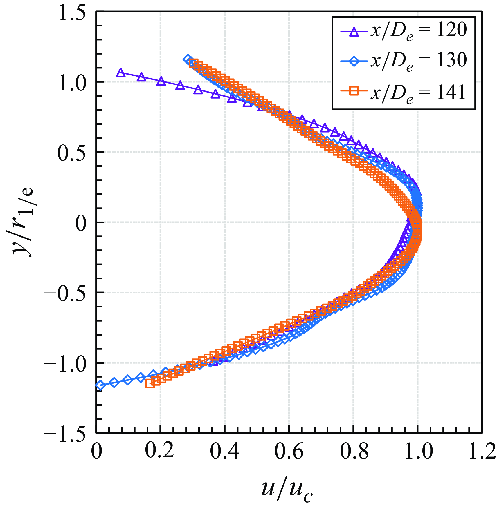
Figure 25. Self-similarity of the normalised streamwise mean velocity profile in the far-field zone.
With self-similarity established in the rarefied free jet, modelling of the centreline velocity in the far-field zone becomes feasible. An incompressible laminar jet can be described by the theoretical equation (Kashi et al. Reference Kashi, Weinberg and Haustein2018)
 \begin{equation} u_{\textit {c}}(x)=u_{\textit {c}}(0)+(0.34-u_{\textit {c}}(0))\left \{ 1-\exp \left [-\frac {12(x-L_{{pc}})}{D_{\textit {e}}\,\textit{Re}_{{D}}}\right ]\right \}, \end{equation}
where $u_{\textit {c}}(0)$
is outlet centreline streamwise velocity normalised by outlet mean velocity (
$u_{\textit {c}}(0)$
is outlet centreline streamwise velocity normalised by outlet mean velocity ( $V_{\textit {e}}$
),
$V_{\textit {e}}$
), $x$
is downstream distance,
$x$
is downstream distance, $L_{{pc}}$
is the potential core length, and
$L_{{pc}}$
is the potential core length, and $\textit{Re}_{{D}}$
is the Reynolds number based on the nozzle diameter. In this study,
$\textit{Re}_{{D}}$
is the Reynolds number based on the nozzle diameter. In this study, $u_{\textit {c}}(0)$
is assigned value 2, as the focus is on the fully developed region.
$u_{\textit {c}}(0)$
is assigned value 2, as the focus is on the fully developed region.
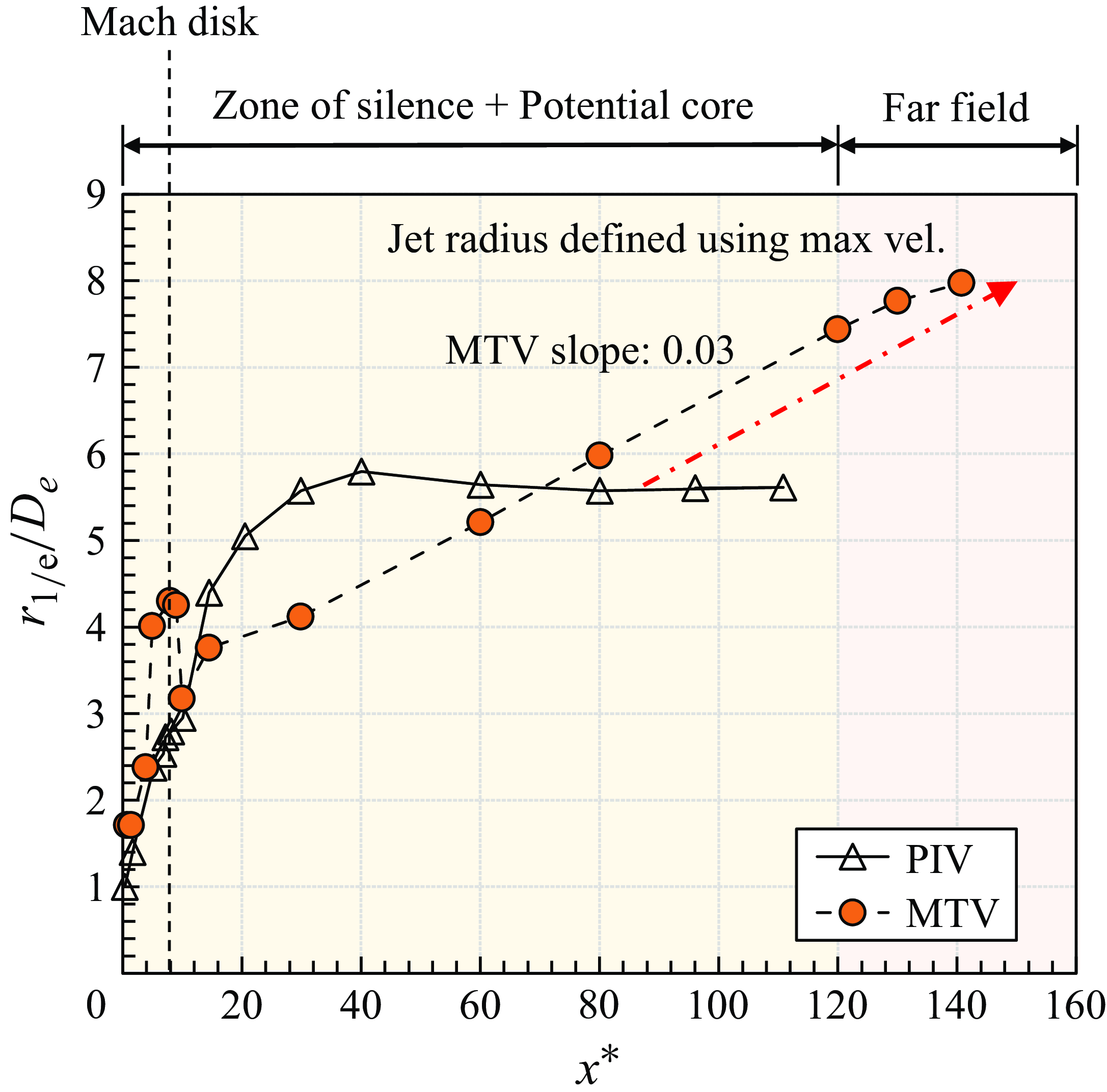
Figure 26. Normalised jet radius defined by the radial distance where the streamwise velocity decreases to $1/e$
of the maximum velocity.
$1/e$
of the maximum velocity.
To establish the characteristic velocity, an analogy was drawn from methodologies employed in the analysis of supersonic turbulent jets, wherein the distinction between total and ambient density is represented as the NPR. The characteristic diameter $D_{{ch}}$
is first defined as
$D_{{ch}}$
is first defined as
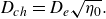 \begin{equation} D_{{ch}}=D_{\textit {e}}\sqrt {\eta _0}. \end{equation}
As per Morton (Reference Morton1967), the complex Reynolds number, which determines the flow regime of the jet, remains constant regardless of the jet region, enabling us to write
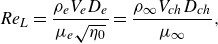 \begin{equation} \textit{Re}_{L}=\frac {\rho _{\textit {e}} V_{\textit {e}} D_{\textit {e}}}{\mu _{\textit {e}}\sqrt {\eta _0}}=\frac {\rho _\infty V_{{ch}} D_{{ch}}}{\mu _\infty }, \end{equation}
where $\rho _{\textit {e}}$
is the exit density,
$\rho _{\textit {e}}$
is the exit density, $V_{\textit {e}}$
is the exit velocity,
$V_{\textit {e}}$
is the exit velocity, $\mu _{\textit {e}}$
is the exit dynamic viscosity,
$\mu _{\textit {e}}$
is the exit dynamic viscosity, $\rho _\infty$
is the ambient density,
$\rho _\infty$
is the ambient density, $V_{{ch}}$
is the characteristic velocity, and
$V_{{ch}}$
is the characteristic velocity, and $\mu _\infty$
is the ambient dynamic viscosity. Rearranging this equation for characteristic velocity gives
$\mu _\infty$
is the ambient dynamic viscosity. Rearranging this equation for characteristic velocity gives $V_{{ch}}=211\ \rm m\ s^{-1}$
, which is used in (4.5) as the outlet mean velocity. As depicted in figure 27, there is good collapse between the experimental results and theoretical values. Notably, while (4.5) is derived for an incompressible laminar jet, it is applicable to the fully developed region of the jet in this study due to the transition to incompressible behaviour. In earlier regions, such as before the Mach disk and within the potential core, the jet exhibits compressible behaviour due to significant density and velocity variations. In contrast, in the fully developed region, the jet gradually stabilises in density and temperature as it equilibrates with the surrounding environment. Consequently, the flow behaves as an incompressible jet, allowing (4.5) to be an appropriate model for this region. Although velocity-induced compressibility effects could persist, the data suggest that such effects are negligible in the fully developed region and do not influence the flow behaviour.
$V_{{ch}}=211\ \rm m\ s^{-1}$
, which is used in (4.5) as the outlet mean velocity. As depicted in figure 27, there is good collapse between the experimental results and theoretical values. Notably, while (4.5) is derived for an incompressible laminar jet, it is applicable to the fully developed region of the jet in this study due to the transition to incompressible behaviour. In earlier regions, such as before the Mach disk and within the potential core, the jet exhibits compressible behaviour due to significant density and velocity variations. In contrast, in the fully developed region, the jet gradually stabilises in density and temperature as it equilibrates with the surrounding environment. Consequently, the flow behaves as an incompressible jet, allowing (4.5) to be an appropriate model for this region. Although velocity-induced compressibility effects could persist, the data suggest that such effects are negligible in the fully developed region and do not influence the flow behaviour.
In summary, this study presents experimental investigations and analyses of free jets across different flow regimes, specifically focusing on supersonic turbulent and supersonic laminar flows. Figure 28 presents a summary schematic of supersonic free jets to facilitate understanding of the experimental findings. Examination of the overall flow structure reveals distinct jet behaviours corresponding to different flow regimes. Notably, as the ambient environment becomes increasingly rarefied, the flow tends to stabilise gradually, transitioning from turbulent to laminar flow. Furthermore, it is observed that the degree of expansion upon flow exit from the sonic nozzle increases with rarefaction. At a distance $x^*= 6$
near the nozzle, it is noted that the jet radius is larger for the 1 torr free jet.
$x^*= 6$
near the nozzle, it is noted that the jet radius is larger for the 1 torr free jet.
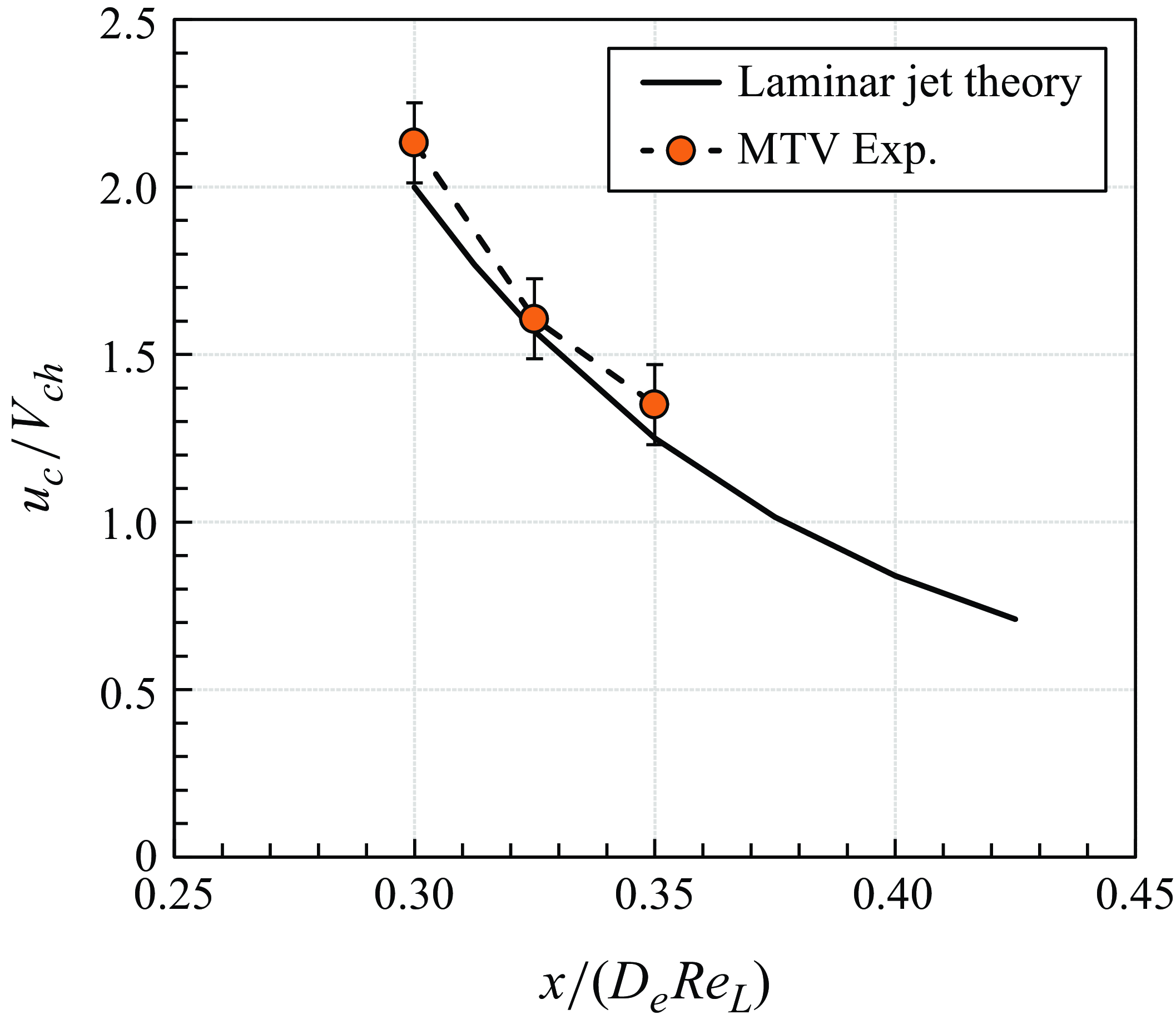
Figure 27. Evolution of normalised centreline streamwise mean velocity in the far-field zone at 1 torr.
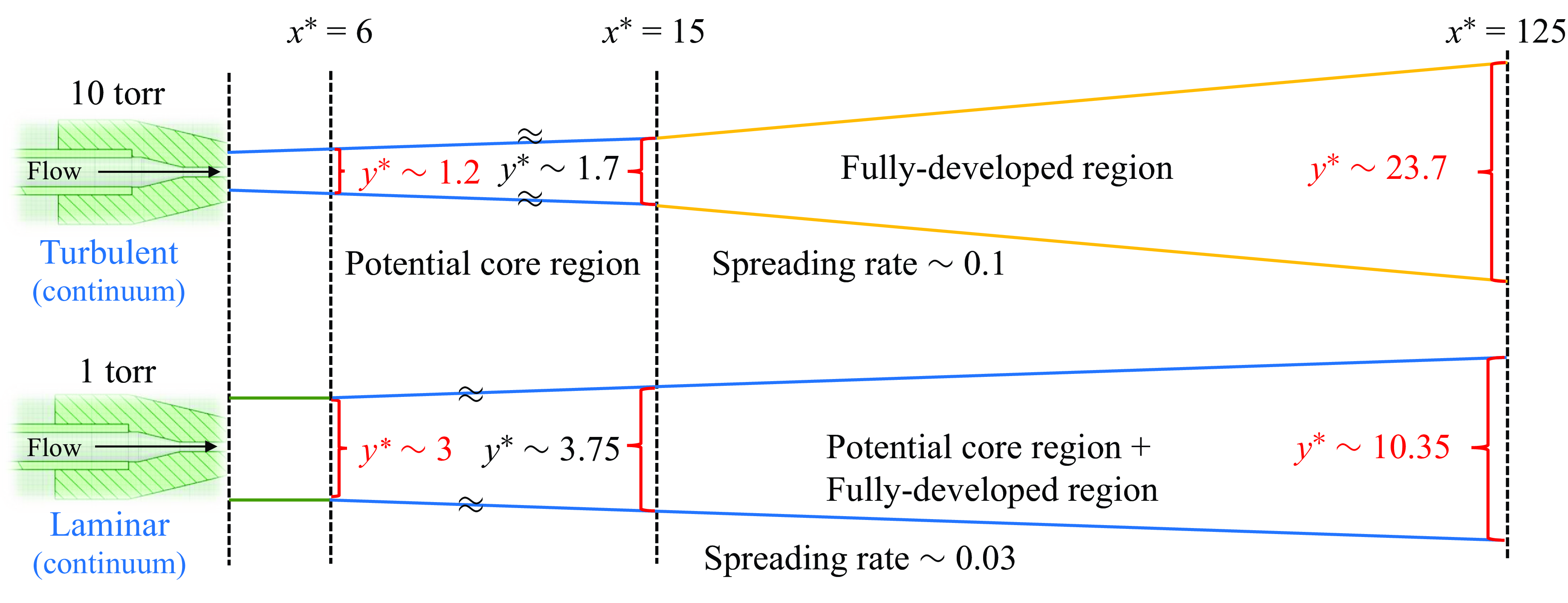
Figure 28. Overall flow structure of supersonic free jets.
As the turbulent jet progresses downstream, it reaches the fully developed region after a short potential core, resulting in a rapid increase in jet profile, with spreading rate 0.1. Conversely, the laminar jet exhibits a lower spreading rate 0.03 for both the potential core and fully developed regions. These factors cause a difference in jet radius, with the laminar jet exhibiting a larger radius in the zone of silence due to the high NPR, while the turbulent jet radius becomes larger in the far-field zone due to its higher spreading rate ( $\sim0.1$
) compared to the laminar jet. This trend is particularly evident at
$\sim0.1$
) compared to the laminar jet. This trend is particularly evident at $x^*= 6$
, 15 and 125. Thus the structure of supersonic free jets undergoes different variations depending on the flow regime.
$x^*= 6$
, 15 and 125. Thus the structure of supersonic free jets undergoes different variations depending on the flow regime.
4.2.4. Theoretical modelling
Jets with a long potential core region are relatively rare, resulting in limited research on modelling their velocity profiles. This study seeks to bridge this gap by analysing how velocity distributions develop beyond the potential core, and proposing a suitable modelling approach. When the NPR is moderate, the potential core region remains short, and beyond this point, the jet velocity profile typically follows a Gaussian distribution due to momentum transfer from the central region through the shear layer. However, in cases with a long potential core region, this distribution modelling becomes inaccurate due to the velocity deceleration across the diameter of the Mach disk. Utilising a bi-modal distribution allows for the effective emulation of the velocity profile, representing both the potential core and fully developed regions. As the standard deviation increases, as shown in figure 29(a), modelling captures the inner and outer shear layers. Beyond a threshold, the two distributions merge into a single Gaussian, representing the fully developed velocity profile, as illustrated in figure 29(b).
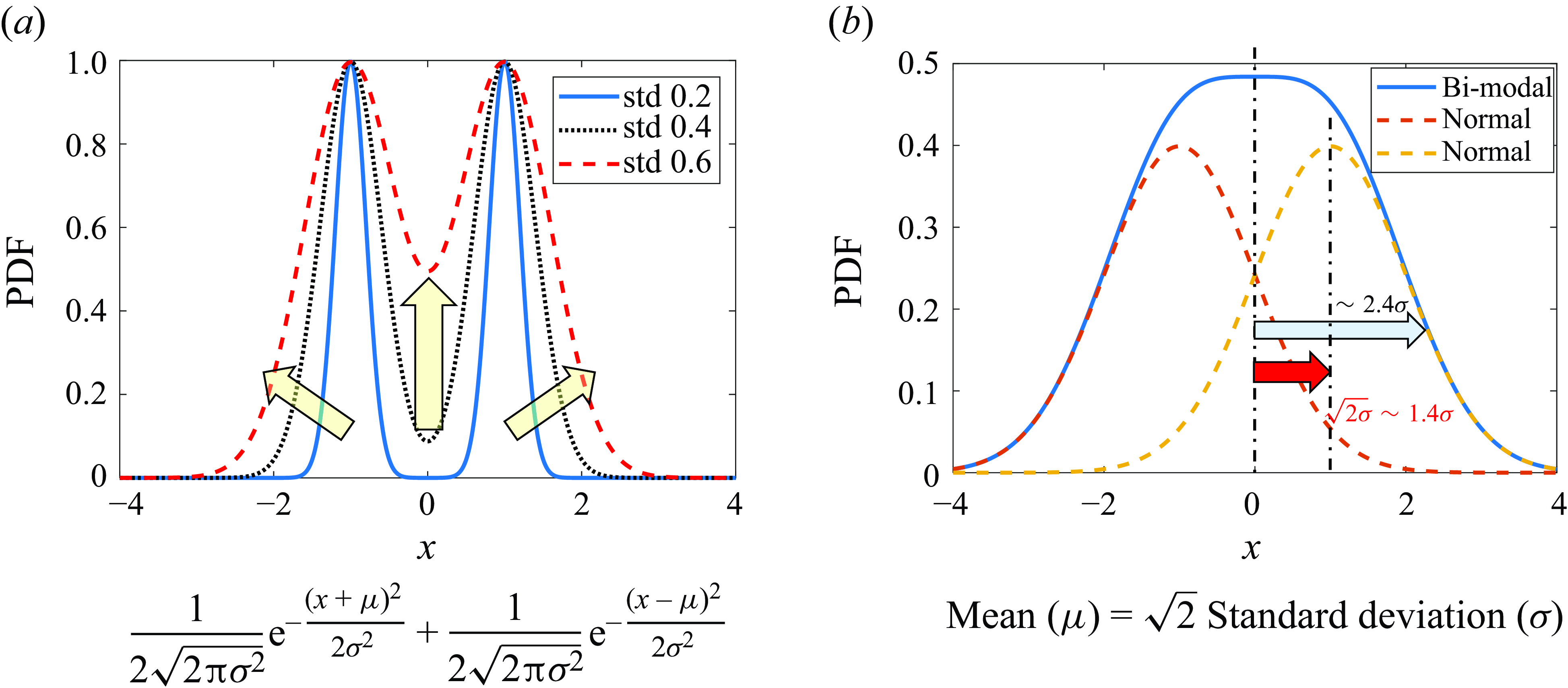
Figure 29. The probability density function (PDF) of the bi-modal distribution: (a) according to standard deviation (std), and (b) convergence into a Gaussian distribution.
A regression can be conducted to fit the experimental data to the bi-modal distribution according to the equation
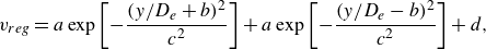 \begin{equation} v_{{reg}}=a\exp {\left [-\frac {(y/D_{\textit {e}}+b)^2}{c^2}\right ]}+a\exp {\left [-\frac {(y/D_{\textit {e}}-b)^2}{c^2}\right ]}+d, \end{equation}
where $v_{{reg}}$
is the regression result of the velocity for a bi-modal distribution centred at 0. The constant a represents the maximum value of the peak, b represents the symmetry origin, and c represents the radius of each jet. A velocity offset d was introduced to improve the fit, ensuring that d never exceeds 10 % of the maximum value of
$v_{{reg}}$
is the regression result of the velocity for a bi-modal distribution centred at 0. The constant a represents the maximum value of the peak, b represents the symmetry origin, and c represents the radius of each jet. A velocity offset d was introduced to improve the fit, ensuring that d never exceeds 10 % of the maximum value of $v_{{reg}}$
. This expression matches the MTV results well, within the measurement uncertainty.
$v_{{reg}}$
. This expression matches the MTV results well, within the measurement uncertainty.
To assess whether the bi-modal distribution effectively models both the potential core and fully developed regions, comparisons were made with MTV experimental results at 1 torr. Figure 30 compares the derived bi-modal distribution with the corresponding experimental data for six locations. As is evident from the regression, the bi-modal distribution effectively models the inner and outer shear layers in the potential core region, while in the fully developed region, the two velocity peaks merge into a Gaussian distribution. This strong fit indicates that the outer and inner shear layers develop through momentum transfer, a mechanism similar to jet evolution in the fully developed region, reinforcing the validity of the model.
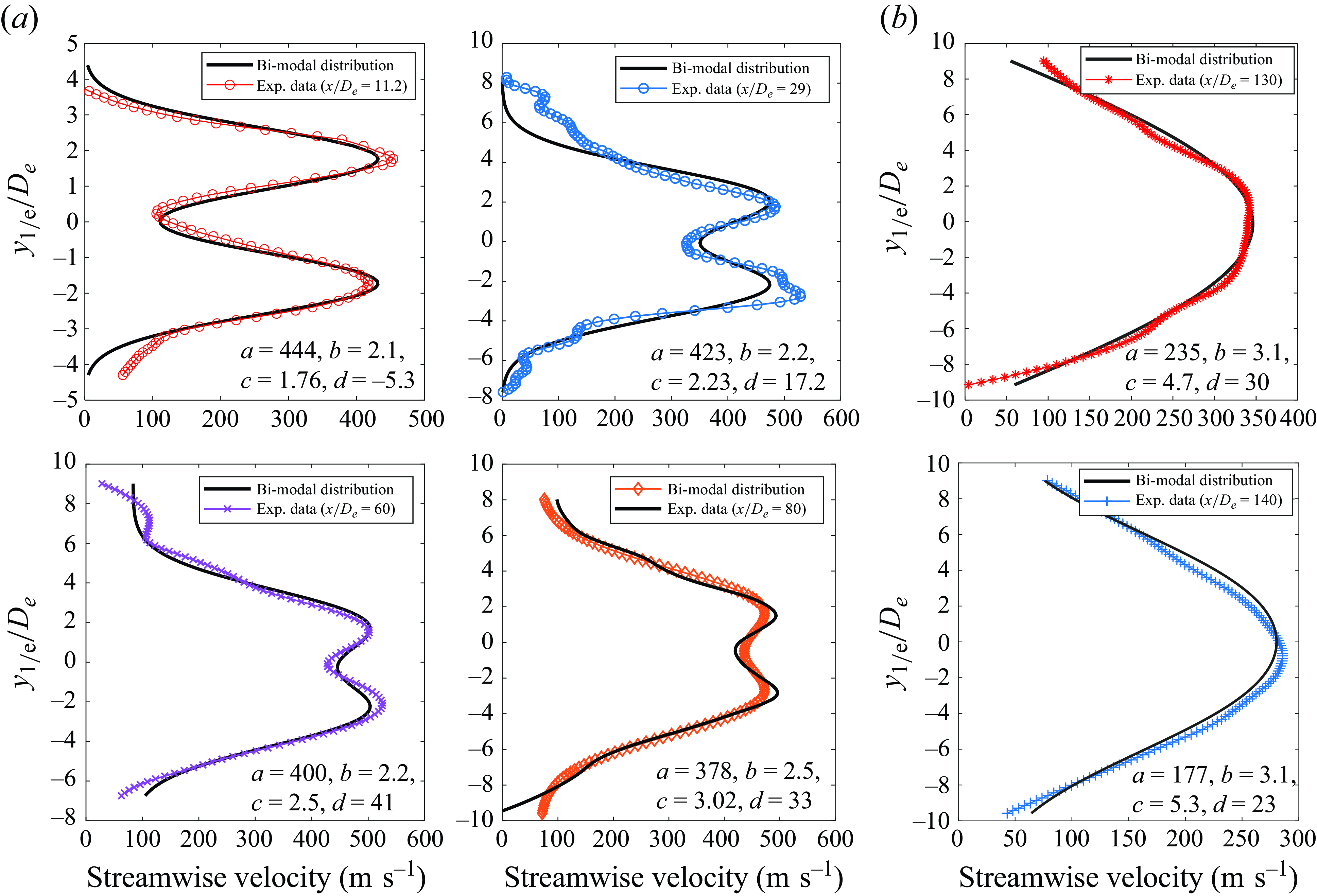
Figure 30. Streamwise mean velocity profiles from the MTV experiments and regression result of bi-modal distribution for (a) the potential core region, and (b) the far-field zone.
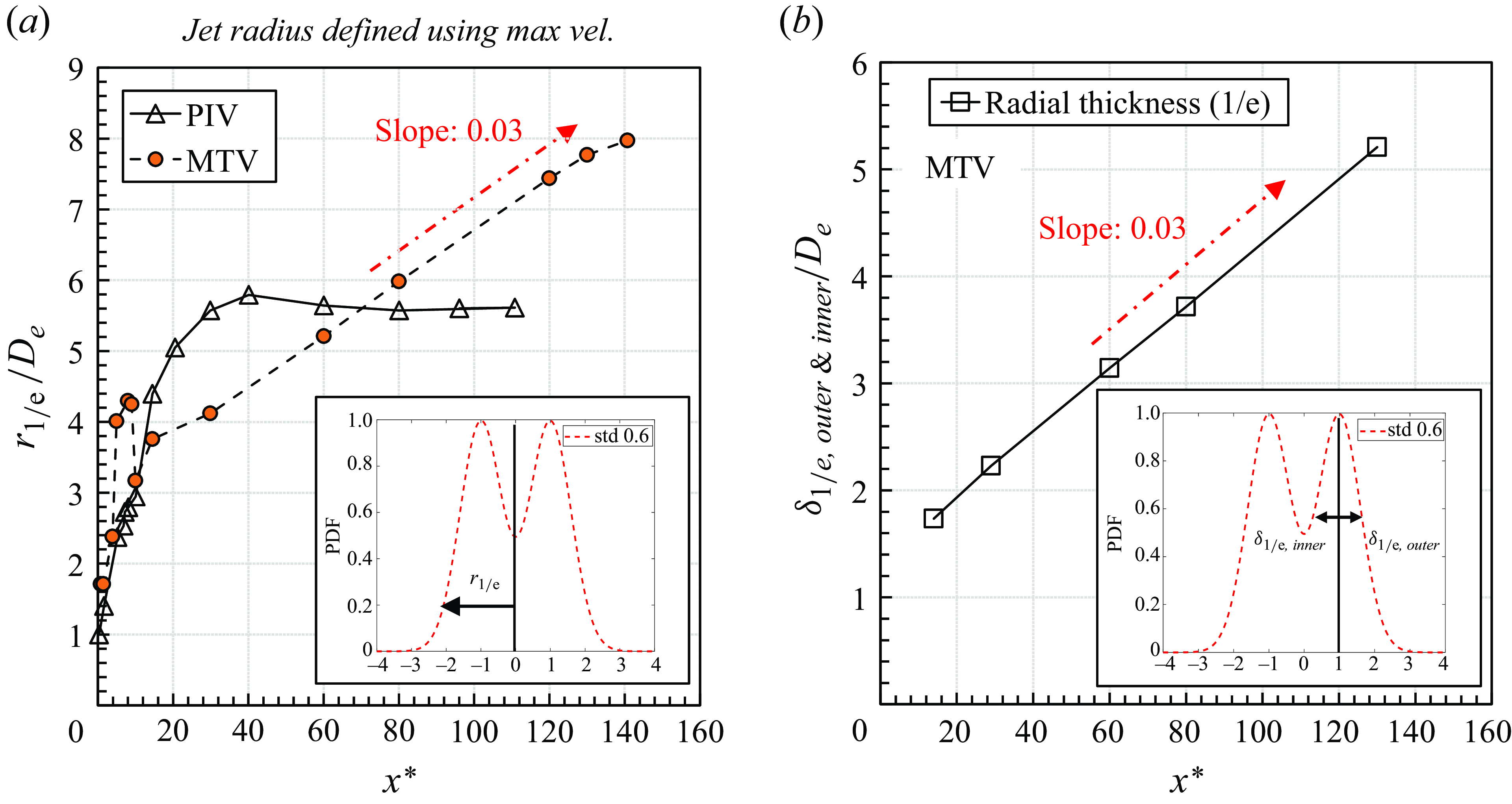
Figure 31. Normalised (a) overall jet radius and (b) inner and outer shear layer radial thickness.
Further analysis involved verifying the development of the jet radius. In figure 31(a), the radius of the entire jet profile was determined based on the $1/e$
criterion of the maximum velocity. In figure 31(b), the radial thickness of the inner and outer shear layers was determined based on the distance from the peak centre in the jet profile. Both radial thicknesses were found to develop at rate 0.03, indicating symmetric development of both the inner and outer shear layers, and also implying that the flow regime was laminar. These results suggest that the bi-modal distribution is adequate in representing the jet profile after the Mach disk.
$1/e$
criterion of the maximum velocity. In figure 31(b), the radial thickness of the inner and outer shear layers was determined based on the distance from the peak centre in the jet profile. Both radial thicknesses were found to develop at rate 0.03, indicating symmetric development of both the inner and outer shear layers, and also implying that the flow regime was laminar. These results suggest that the bi-modal distribution is adequate in representing the jet profile after the Mach disk.
By observing that both the inner and outer shear layers grow similarly to the overall jet profile following a bi-modal distribution, it becomes possible to estimate the length of the potential core region. Empirical correlations exist for determining the position and size of the Mach disk experimentally ((4.2) and (4.3)). The distance between the dual peaks of the bi-modal distribution is equivalent to the Mach disk size, as confirmed by MTV experimental data (refer to Appendix E). Additionally, the inner shear layer develops downstream following the laminar jet spreading rate. For the bi-modal distribution to transition to a Gaussian distribution, the inner shear layer must develop a distance $\sqrt {2}$
times half of the Mach disk size, as depicted in figure 29(b). Utilising this information and the definition of the spreading rate, it is possible to determine how much development length is required for the bi-modal distribution to transition to a Gaussian distribution, using the equation
$\sqrt {2}$
times half of the Mach disk size, as depicted in figure 29(b). Utilising this information and the definition of the spreading rate, it is possible to determine how much development length is required for the bi-modal distribution to transition to a Gaussian distribution, using the equation
 \begin{equation} \frac {12}{\textit{Re}_L}=\frac {0.37\sqrt {2}D_{\textit {e}}\eta _0^{0.5}/2}{\textrm {potential core length}\ (PCL)- \textrm {distance of Mach disk}\ (DMD)\ \textrm {from nozzle exit}}. \end{equation}
Rearranging (4.9) for PCL, and normalising by nozzle diameter, gives
 \begin{equation} PCL_{{lam}}^*=\frac {DMD}{D_{\textit {e}}}+\frac {0.37\sqrt {2}\,\textit{Re}_L\,\eta _0^{0.5}}{24}=0.64\,\eta _0^{0.5}+0.022\,\textit{Re}_L\,\eta _0^{0.5}. \end{equation}
This equation is applicable within the laminar flow regime where the complex Reynolds number ranges from 100 to 1000, and is limited to extremely under-expanded supersonic jets with a single barrel shock. Similarly, for turbulent jets under the same conditions, where $\textit{Re}_L \gt O(10^4)$
and spreading rate 0.1 is assumed, the equation is modified by replacing
$\textit{Re}_L \gt O(10^4)$
and spreading rate 0.1 is assumed, the equation is modified by replacing $12/\textit{Re}_L$
in (4.9) with 0.1, yielding the result
$12/\textit{Re}_L$
in (4.9) with 0.1, yielding the result
 \begin{equation} PCL_{{turb}}^*=0.64\,\eta _0^{0.5}+1.85\sqrt {2}\,\eta _0^{0.5}. \end{equation}
These newly developed correlations are first validated against experimental data across turbulent, laminar and rarefied flow regimes, demonstrating an accuracy within 10 %. While errors slightly increased in the rarefied regime, likely due to Mach disk thickening (Volchkov et al. Reference Volchkov, Ivanov, Kislyakov, Rebrov, Sukhnev and Sharafutdinov1973), the correlation remained reliable across a broad range of conditions. In contrast, Phalnikar’s widely used relation (Phalnikar, Kumar & Alvi Reference Phalnikar, Kumar and Alvi2008), which estimates the supersonic core length as $SCL^*= 1.8\eta _{0} + 2.9$
, showed significant errors in predicting the normalised potential core length, as shown in table 6. Although the supersonic core extends slightly beyond the potential core, their difference is minor, making it a reasonable comparison metric. However, Phalnikar’s relation, derived from empirical data with NPR less than 8, fails at higher NPR values due to unaccounted changes in shockwave structures and flow regimes. By capturing these effects, the present correlation provides a more accurate representation across a wider range of supersonic free jets, including extremely under-expanded free jets with high pressure ratios and one-barrel shockwaves (Fond et al. Reference Fond, Xiao, T’Joen, Henkes, Veenstra, van Wachem and Beyrau2018; Bykov et al. Reference Bykov, Gorbachev and Fyodorov2023).
$SCL^*= 1.8\eta _{0} + 2.9$
, showed significant errors in predicting the normalised potential core length, as shown in table 6. Although the supersonic core extends slightly beyond the potential core, their difference is minor, making it a reasonable comparison metric. However, Phalnikar’s relation, derived from empirical data with NPR less than 8, fails at higher NPR values due to unaccounted changes in shockwave structures and flow regimes. By capturing these effects, the present correlation provides a more accurate representation across a wider range of supersonic free jets, including extremely under-expanded free jets with high pressure ratios and one-barrel shockwaves (Fond et al. Reference Fond, Xiao, T’Joen, Henkes, Veenstra, van Wachem and Beyrau2018; Bykov et al. Reference Bykov, Gorbachev and Fyodorov2023).
Table 6. Comparison of potential core length.
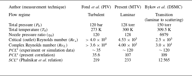
5. Conclusion
Previous research into supersonic jet flows occurring in rarefied gas conditions has focused predominantly on the near-field zone, with limited emphasis on quantitative flow velocity measurement or analysis in the far-field zone. However, flow characteristics in the far-field zone undergo substantial changes, necessitating a thorough understanding of their behaviour.
In this study, we established a robust experimental foundation for understanding the flow field of a rarefied supersonic free jet within the laminar and turbulent flow regimes, encompassing both near-field and far-field zones. Utilising nanometre-sized tracer particles for particle image velocimetry (PIV), and acetone molecules for molecular tagging velocimetry (MTV), distinct flow characteristics were revealed. In the highly under-expanded regime characterised by turbulent flow, the supersonic jet exhibited a cyclical shockwave structure in the near-field zone, followed by a relatively short potential core region. The far-field zone exhibited the spreading rate, decay constant and turbulence statistics of a turbulent jet, and additionally satisfied self-similarity. As the nozzle pressure ratio (NPR) increased, the near-field zone exhibited a single-barrel shockwave structure, while the far-field zone transitioned into a laminar flow regime, consistent with theoretical predictions based on complex Reynolds numbers. The velocity near the Mach disk significantly decreased, and the shear layer developed slowly in the laminar flow regime, resulting in an extended potential core region. Beyond the potential core, a fully-developed region was reached, satisfying self-similarity in accordance with laminar jet theory. Additionally, we modelled the velocity profile after the Mach disk with a one-barrel shockwave structure in the laminar flow regime using a bi-modal distribution. This was found to accurately replicate the inner and outer shear layers, and merges into a normal distribution after the shear layers converge. Through this analysis, we developed a new correlation to estimate the potential core length based on NPR and complex Reynolds number.
The significance of this work is fourfold. First, the experiments represent the first quantitative measurement of the velocity profile in the far-field zone of a supersonic free jet in rarefied conditions utilising MTV. Second, this study provides experimental evidence of the inability of particles to accurately follow supersonic flow in rarefied environments by quantitatively comparing PIV and MTV results. This demonstrates that relying solely on the Stokes number at the nozzle outlet is insufficient for determining the applicability of PIV in such conditions. Third, the theoretical significance is highlighted by the observation and modelling of a long annular shear layer developing in the laminar flow regime following the Mach disk. This deviation from typical turbulent jet characteristics underscores the necessity for a more thorough understanding of flow dynamics in extreme environments. Fourth, from an application perspective, these findings provide insights for designing key devices in semiconductor and aerospace industries, such as showerheads, micro-throttles or lunar landing systems.
Looking ahead, future work will focus on expanding the scope of this research to encompass multi-hole jet configurations. Considering that many applications have multiple jets originating from several outlets, understanding jet-to-jet interaction is crucial for capturing the complexities of supersonic free jets. As shockwave structures become more intricate, the influence of multi-hole configurations on the far-field flow dynamics must also be thoroughly investigated.
Funding
This work was supported by the National Research Foundation of Korea (NRF) grant funded by the Korea government (MSIT) (No. RS-2024-00346766 and RS-2024-00406514) and Samsung Electronics (RRH0120ZZ-04RF). Additionally, this work was supported by the Institute of Advanced Machines and Design, and the Institute of Engineering Research at Seoul National University.
Declaration of interests
The authors report no conflict of interest.
Author contributions
H.P.: conceptualisation, data curation, formal analysis, investigation, methodology, software, validation, visualisation, writing – original draft. S.L.: data curation, formal analysis, methodology, software. W.H.: project administration, funding acquisition, resources, supervision, writing – review and editing.
Data availability statement
All relevant data are within the paper.
Appendix A. Derivation of complex Reynolds number in major regions of the jet
Based on the research of Volchkov et al. (Reference Volchkov, Ivanov, Kislyakov, Rebrov, Sukhnev and Sharafutdinov1973), we can define a Reynolds number at each major area in the extremely under-expanded supersonic free jet depicted in figure 1(b). The flow field is delineated into three main areas: the zone of silence before the Mach disk (region 1), the area following the Mach disk (region 2), and the annular shear layer unaffected by the Mach disk (region 3).
In region 1, the jet core region, bounded by the barrel shock and the Mach disk, the variation of the viscosity coefficient with temperature follows $\mu \sim T^w$
, where
$\mu \sim T^w$
, where $\mu$
represents the dynamic viscosity,
$\mu$
represents the dynamic viscosity, $T$
is the static temperature, and
$T$
is the static temperature, and $w$
is an exponent defining the temperature dependence. In this zone, the density
$w$
is an exponent defining the temperature dependence. In this zone, the density $\rho _1$
near the jet axis and far from the nozzle where the velocity
$\rho _1$
near the jet axis and far from the nozzle where the velocity $u_1$
approaches its maximum is given by
$u_1$
approaches its maximum is given by $\rho _1/\rho _0 = B D_{{e}}^2/x^2$
, where
$\rho _1/\rho _0 = B D_{{e}}^2/x^2$
, where $\rho _0$
is the density in the nozzle’s forechamber,
$\rho _0$
is the density in the nozzle’s forechamber, $x$
is the distance from the nozzle outlet, and
$x$
is the distance from the nozzle outlet, and $B = B(\gamma , M)$
is a coefficient dependent on the specific heat ratio
$B = B(\gamma , M)$
is a coefficient dependent on the specific heat ratio $\gamma$
and Mach number
$\gamma$
and Mach number $M$
. The characteristic length scale in this region, represented by the distance to the Mach disk
$M$
. The characteristic length scale in this region, represented by the distance to the Mach disk $L_{{M}}$
, is expressed as
$L_{{M}}$
, is expressed as $L_{{M}} = 0.67 D_{{e}} \sqrt {\eta _0}$
, where
$L_{{M}} = 0.67 D_{{e}} \sqrt {\eta _0}$
, where $D_{\textit {e}}$
is the nozzle diameter, and
$D_{\textit {e}}$
is the nozzle diameter, and $\eta _0$
is the pressure ratio between the total pressure
$\eta _0$
is the pressure ratio between the total pressure $P_0$
and the ambient pressure
$P_0$
and the ambient pressure $P_{\infty }$
(Sherman Reference Sherman1966). The Reynolds number in region 1, denoted as
$P_{\infty }$
(Sherman Reference Sherman1966). The Reynolds number in region 1, denoted as $\textit{Re}_1$
, is calculated using
$\textit{Re}_1$
, is calculated using $\textit{Re}_1 \sim M^{2w}\, \textit{Re}_*/\sqrt {\eta _0}$
, where
$\textit{Re}_1 \sim M^{2w}\, \textit{Re}_*/\sqrt {\eta _0}$
, where $\textit{Re}_*$
is the Reynolds number based on the nozzle throat diameter. Dissipative effects are characterised by the local Knudsen number, defined as
$\textit{Re}_*$
is the Reynolds number based on the nozzle throat diameter. Dissipative effects are characterised by the local Knudsen number, defined as $Kn_1 \sim \sqrt {\eta _0}/\textit{Re}_*$
. The dimensionless parameter
$Kn_1 \sim \sqrt {\eta _0}/\textit{Re}_*$
. The dimensionless parameter $\textit{Re}_*/{\sqrt {\eta _0}}$
is useful for analysing the effects of viscosity, thermal conduction and molecular energy relaxation processes in the jet core.
$\textit{Re}_*/{\sqrt {\eta _0}}$
is useful for analysing the effects of viscosity, thermal conduction and molecular energy relaxation processes in the jet core.
In region 2 after the Mach disk, the characteristic dimension is the Mach disk diameter $D_{{M}}$
, and the Reynolds number in this region is calculated as
$D_{{M}}$
, and the Reynolds number in this region is calculated as $\textit{Re}_2 \sim \rho _2 u_2 D_{\textit {M}}/\mu _2$
, where
$\textit{Re}_2 \sim \rho _2 u_2 D_{\textit {M}}/\mu _2$
, where $\rho _2$
represents the average density,
$\rho _2$
represents the average density, $u_2$
is the average velocity, and
$u_2$
is the average velocity, and $\mu _2$
is the average dynamic viscosity in region 2. For large pressure ratios (
$\mu _2$
is the average dynamic viscosity in region 2. For large pressure ratios ( $\eta _0 \gg 1$
), the approximations
$\eta _0 \gg 1$
), the approximations $\mu _2 \sim \mu _{\textit {e}}$
,
$\mu _2 \sim \mu _{\textit {e}}$
, $u_2 \sim u_{{e}}/U_{max }$
and
$u_2 \sim u_{{e}}/U_{max }$
and $ \rho _2 \sim (\gamma +1) B \rho _0 D_{\textit {e}}^2/(\gamma -1) L_{\textit {M}}^2$
hold true. Given that
$ \rho _2 \sim (\gamma +1) B \rho _0 D_{\textit {e}}^2/(\gamma -1) L_{\textit {M}}^2$
hold true. Given that $D_{{M}} \sim D_{{e}} \sqrt {\eta _0}$
and
$D_{{M}} \sim D_{{e}} \sqrt {\eta _0}$
and $L_{{M}} \sim D_{{e}} \sqrt {\eta _0}$
, the Reynolds number simplifies to
$L_{{M}} \sim D_{{e}} \sqrt {\eta _0}$
, the Reynolds number simplifies to $\textit{Re}_2 \sim \textit{Re}_*/\sqrt {\eta _0}$
.
$\textit{Re}_2 \sim \textit{Re}_*/\sqrt {\eta _0}$
.
Finally, in region 3, which refers to the mixing layer after the barrel shock, the Reynolds number is defined as $\textit{Re}_3 \sim \rho _3 u_3 \varDelta /\mu _3$
, where
$\textit{Re}_3 \sim \rho _3 u_3 \varDelta /\mu _3$
, where $\rho _3$
is the average density,
$\rho _3$
is the average density, $u_3$
is the average velocity,
$u_3$
is the average velocity, $\varDelta$
is the thickness, and
$\varDelta$
is the thickness, and $\mu _3$
is the average dynamic viscosity of the mixing layer. At large distances from the nozzle, where the annular layer dominates the flow rate, the continuity equation helps to approximate
$\mu _3$
is the average dynamic viscosity of the mixing layer. At large distances from the nozzle, where the annular layer dominates the flow rate, the continuity equation helps to approximate $\rho _3 u_3 \sim {\rho _{\textit {e}} u_{\textit {e}} D_{\textit {e}}^2/D_{\textit {M}}\Delta }$
. Given that
$\rho _3 u_3 \sim {\rho _{\textit {e}} u_{\textit {e}} D_{\textit {e}}^2/D_{\textit {M}}\Delta }$
. Given that $D_{{M}} \sim D_{{e}} \sqrt {\eta _0}$
and
$D_{{M}} \sim D_{{e}} \sqrt {\eta _0}$
and $\varDelta \sim D_{{e}} \sqrt {\eta _0}$
, we obtain
$\varDelta \sim D_{{e}} \sqrt {\eta _0}$
, we obtain $\textit{Re}_3 \sim {\mu _0\, \textit{Re}_*/\mu _3 \sqrt {\eta _0}}$
. This leads to
$\textit{Re}_3 \sim {\mu _0\, \textit{Re}_*/\mu _3 \sqrt {\eta _0}}$
. This leads to $\textit{Re}_3 \sim ({T_0/T_3} )^w\, {\textit{Re}_*/\sqrt {\eta _0}}$
, where
$\textit{Re}_3 \sim ({T_0/T_3} )^w\, {\textit{Re}_*/\sqrt {\eta _0}}$
, where $T_0$
is the stagnation temperature, and
$T_0$
is the stagnation temperature, and $T_3$
is the static temperature in the mixing layer. For congruent cross-sections where
$T_3$
is the static temperature in the mixing layer. For congruent cross-sections where $T_0 \approx T_3$
, the Reynolds number simplifies to
$T_0 \approx T_3$
, the Reynolds number simplifies to $\textit{Re}_3 \sim {\textit{Re}_*}/\sqrt {\eta _0}$
.
$\textit{Re}_3 \sim {\textit{Re}_*}/\sqrt {\eta _0}$
.
In conclusion, for all three zones, the local Reynolds numbers consistently scale with ${\textit{Re}_*}/{\sqrt {\eta _0}}$
, making this ratio the fundamental criterion for describing viscosity, thermal conduction and relaxation effects.
${\textit{Re}_*}/{\sqrt {\eta _0}}$
, making this ratio the fundamental criterion for describing viscosity, thermal conduction and relaxation effects.
Appendix B. Thermophysical property variation
In this appendix, the influence of the variation in thermophysical properties resulting from seeding acetone as a tracer molecule for the MTV experiments in quasi-vacuum conditions is examined. The MTV technique is widely employed in fluid mechanics research, which provides valuable insights into velocity profiles and flow characteristics. However, the addition of acetone as seed introduces complexities due to the distinct thermophysical properties compared to the base gas of nitrogen used in the experiments. To accurately interpret the MTV data and account for the effects of acetone seeding, a comprehensive understanding of the variation in thermophysical properties is essential.
Some studies (Handa et al. Reference Handa, Masuda, Kashitani and Yamaguchi2011; Sakurai et al. Reference Sakurai, Handa, Koike, Mii and Nakano2015) have controlled the acetone concentration to below 1 % and assumed minimal impact from seeding. However, typically when seeding acetone using a bubbler or aerosol generator, it is challenging to precisely determine the concentration. Thus prior studies (Huffman & Elliott Reference Huffman and Elliott2009; Gragston & Smith Reference Gragston and Smith2022; Andrade et al. Reference Andrade, Hoffman, LaLonde and Combs2022) utilising acetone have assumed full saturation at the given total temperature and pressure, and analysed the effect of maximum acetone seeding. In our study, we also assumed full saturation and analysed its effects.
First, the saturated pressure at 300 K was calculated using the Antoine equation below and is shown in figure 32, with seeding performed at 300 K and 760 torr in an $\mathrm{N}_{2}$
positive chamber:
$\mathrm{N}_{2}$
positive chamber:
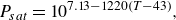 \begin{equation} P_{{sat}}= 10^{7.13-1220(T-43)}, \end{equation}
where $P_{{sat}}$
is acetone saturated vapour pressure (torr), and
$P_{{sat}}$
is acetone saturated vapour pressure (torr), and $T$
is temperature (
$T$
is temperature ( $K$
). Based on this equation, the
$K$
). Based on this equation, the $\mathrm{N}_{2}$
to acetone gas ratio was found to be 67 : 33, allowing calculation of the mixture’s specific heat using Dalton’s law:
$\mathrm{N}_{2}$
to acetone gas ratio was found to be 67 : 33, allowing calculation of the mixture’s specific heat using Dalton’s law:
 \begin{align} C_{p,mix}= m_{\mathrm{C_{3}H_{6}O}}\, C_{p,\mathrm{C_{3}H_{6}O}}+(1- m_{\mathrm{C_{3}H_{6}O}})\,C_{p,\mathrm{N_2}},\end{align}
 \begin{align} C_{v,mix}= m_{\mathrm{C_{3}H_{6}O}}\,C_{v,\mathrm{C_{3}H_{6}O}}+(1- m_{\mathrm{C_{3}H_{6}O}})\, C_{v,\mathrm{N_2}},\end{align}
where $C_{p}$
and
$C_{p}$
and $C_{v}$
are constant pressure and volume specific heats, respectively, and
$C_{v}$
are constant pressure and volume specific heats, respectively, and $m$
is mole fraction of the species. Additionally, density and dynamic viscosity were calculated to obtain the mixture density and dynamic viscosity (Faghri & Zhang Reference Faghri and Zhang2006), crucial for understanding the influence of acetone on the complex Reynolds number. Following acetone seeding, as seen in table 7, the specific heat ratio slightly decreased to 1.3, remaining constant at both 10 and 1 torr. The complex Reynolds number, as shown in table 8, slightly increased from 1300 to 1400 at 10 torr, and from 400 to 430 at 1 torr. However, these variations had minimal impact on the jet flow regime, with little change observed in spreading rates, particularly in the laminar flow regime.
$m$
is mole fraction of the species. Additionally, density and dynamic viscosity were calculated to obtain the mixture density and dynamic viscosity (Faghri & Zhang Reference Faghri and Zhang2006), crucial for understanding the influence of acetone on the complex Reynolds number. Following acetone seeding, as seen in table 7, the specific heat ratio slightly decreased to 1.3, remaining constant at both 10 and 1 torr. The complex Reynolds number, as shown in table 8, slightly increased from 1300 to 1400 at 10 torr, and from 400 to 430 at 1 torr. However, these variations had minimal impact on the jet flow regime, with little change observed in spreading rates, particularly in the laminar flow regime.

Figure 32. Acetone saturated vapour pressure calculated from the Antoine equation.
Table 7. Thermophysical property variation with acetone seeding.
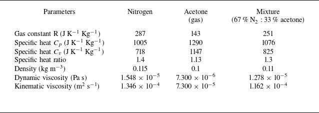
Table 8. Reynolds number variation with acetone seeding.
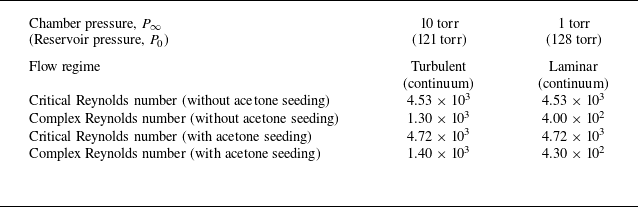
Appendix C. Evolution of the Stokes number in the zone of silence
The Stokes number is defined as $\tau _{p}/\tau_f$
, where
$\tau _{p}/\tau_f$
, where $\tau _{p}$
is the particle relaxation time scale, and
$\tau _{p}$
is the particle relaxation time scale, and $\tau _{f}$
is a fluid time scale. The particle relaxation time scale is defined as
$\tau _{f}$
is a fluid time scale. The particle relaxation time scale is defined as
 \begin{equation} \tau _p=\frac {\rho _p d_p^2}{18\mu _f}, \end{equation}
where $\rho _p$
,
$\rho _p$
, $d_{p}$
and
$d_{p}$
and $\mu _{f}$
are the particle density, diameter and fluid dynamic viscosity, respectively. In the case of the fluid time scale, it can be obtained using the mean velocity magnitude at the nozzle outlet and nozzle diameter.
$\mu _{f}$
are the particle density, diameter and fluid dynamic viscosity, respectively. In the case of the fluid time scale, it can be obtained using the mean velocity magnitude at the nozzle outlet and nozzle diameter.
To account for the rarefied gas conditions in the downstream region, the Cunningham correction factor (Cunningham Reference Cunningham1910; Davies Reference Davies1945) $C_c$
is used to correct the Stokes number, taking into account the molecular mean free path as a constant multiplier that is defined as
$C_c$
is used to correct the Stokes number, taking into account the molecular mean free path as a constant multiplier that is defined as
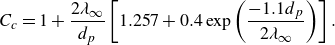 \begin{equation} C_c=1+\frac {2\lambda _\infty }{d_p}\left [1.257+0.4\exp \left (\frac {-1.1d_p}{2\lambda _\infty }\right )\right ]. \end{equation}
The molecular mean free path ( $\lambda _\infty$
) is given by
$\lambda _\infty$
) is given by
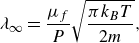 \begin{equation} \lambda _\infty =\frac {\mu _f}{P}\sqrt {\frac {\pi {k_B}T}{2m}}, \end{equation}
where $P$
,
$P$
, $k_B$
,
$k_B$
, $T$
and
$T$
and $m$
are static pressure, Boltzmann constant, static temperature and molecular mass, respectively. In the zone of silence up to the Mach disk, the normalised static temperature and pressure can be computed using equations provided by Morse (Reference Morse1996). Additionally, fluid dynamic viscosity was determined using the NIST Standard Reference Database (Linstrom et al. 2005). These values allowed for the calculation of the mean free path as a function of normalised streamwise distance, which was then used to compute the Cunningham correction factor. The local Stokes number, incorporating the Cunningham correction factor, is expressed as
$m$
are static pressure, Boltzmann constant, static temperature and molecular mass, respectively. In the zone of silence up to the Mach disk, the normalised static temperature and pressure can be computed using equations provided by Morse (Reference Morse1996). Additionally, fluid dynamic viscosity was determined using the NIST Standard Reference Database (Linstrom et al. 2005). These values allowed for the calculation of the mean free path as a function of normalised streamwise distance, which was then used to compute the Cunningham correction factor. The local Stokes number, incorporating the Cunningham correction factor, is expressed as
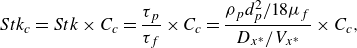 \begin{equation} Stk_c=Stk \times C_c=\frac {\tau _p}{\tau _f}\times C_c=\frac {{\rho _p d_p^2}/{18\mu _f}}{D_{x^*}/V_{x^*}}\times C_c, \end{equation}
where $D_{x^*}$
is the characteristic length at
$D_{x^*}$
is the characteristic length at $x^*$
, and
$x^*$
, and $V_{x^*}$
is the characteristic velocity at
$V_{x^*}$
is the characteristic velocity at $x^*$
. To determine the fluid time scale, the characteristic length and velocity were derived based on mass conservation, as there is no entrainment flow in the zone of silence:
$x^*$
. To determine the fluid time scale, the characteristic length and velocity were derived based on mass conservation, as there is no entrainment flow in the zone of silence:
 \begin{equation} \rho _{\textit {e}} D_{\textit {e}} V_{\textit {e}} \sim \rho _{x^*}D_{x^*}V_{x^*}. \end{equation}
Here, $\rho _{\textit {e}}$
,
$\rho _{\textit {e}}$
, $D_{\textit {e}}$
,
$D_{\textit {e}}$
, $V_{\textit {e}}$
and
$V_{\textit {e}}$
and $\rho _{x^*}$
denote exit density, nozzle diameter, exit velocity and density at
$\rho _{x^*}$
denote exit density, nozzle diameter, exit velocity and density at $x^*$
, respectively. The density at
$x^*$
, respectively. The density at $x^*$
was calculated using relations from Morse (Reference Morse1996), while
$x^*$
was calculated using relations from Morse (Reference Morse1996), while $V_{x^*}$
was defined as the centreline velocity, which increases spherically with distance from the nozzle outlet. The final expression for the Stokes number, incorporating the Cunningham correction factor, is given by
$V_{x^*}$
was defined as the centreline velocity, which increases spherically with distance from the nozzle outlet. The final expression for the Stokes number, incorporating the Cunningham correction factor, is given by
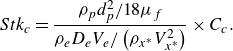 \begin{equation} Stk_c=\frac {{\rho _p d_p^2}/{18\mu _f}}{\rho _{\textit {e}} D_{\textit {e}} V_{\textit {e}}/\left ({\rho _{x^*}}V_{x^*}^2\right )} \times C_c. \end{equation}
Using this equation, the variation of the local Stokes number with normalised streamwise distance is shown in figure 33. A rapid increase in the local Stokes number is observed shortly after the jet discharge. Exceeding unity at $x^* \sim 2$
, this indicates that PIV tracers fail to accurately follow the flow beyond this point.
$x^* \sim 2$
, this indicates that PIV tracers fail to accurately follow the flow beyond this point.
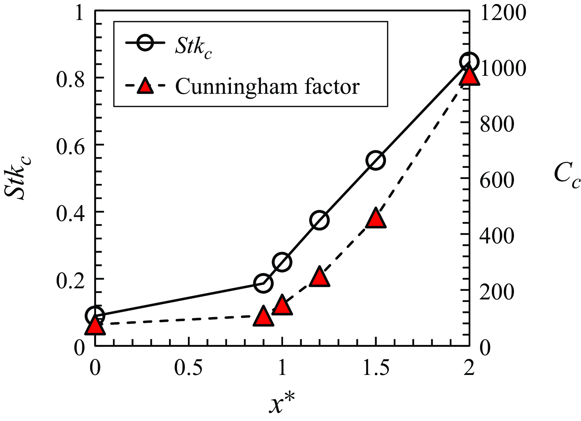
Figure 33. Evolution of local Stokes number and Cunningham factor in the zone of silence.
Most prior studies (Schrijer, Scarano & Van Oudheusden Reference Schrijer, Scarano and Van Oudheusden2006; Mitchell, Honnery & Soria Reference Mitchell, Honnery and Soria2013; De Gregorio Reference De Gregorio2014; André et al. Reference André, Castelain and Bailly2014; Edgington-Mitchell et al. Reference Edgington-Mitchell, Oberleithner, Honnery and Soria2014a
) on supersonic free jets have involved NPR below 10, where $x^*$
typically remains below 2, allowing successful PIV measurements. Even in cases with NPR exceeding 100, such as the jet operating at total pressure 120 bar studied by Fond et al. (Reference Fond, Xiao, T’Joen, Henkes, Veenstra, van Wachem and Beyrau2018), the mean free path was small enough for PIV to succeed. However, in the current study, with NPR exceeding 100 and operating in a rarefied environment, the local Stokes number increases exponentially, which makes it very difficult for PIV tracers to follow the flow accurately. This observation aligns with findings from prior research (Huffman & Elliott Reference Huffman and Elliott2009; Glazyrin, Mursenkova & Znamenskaya Reference Glazyrin, Mursenkova and Znamenskaya2015; Sakurai et al. Reference Sakurai, Handa, Koike, Mii and Nakano2015; Williams et al. Reference Williams, Nguyen, Schreyer and Smits2015).
$x^*$
typically remains below 2, allowing successful PIV measurements. Even in cases with NPR exceeding 100, such as the jet operating at total pressure 120 bar studied by Fond et al. (Reference Fond, Xiao, T’Joen, Henkes, Veenstra, van Wachem and Beyrau2018), the mean free path was small enough for PIV to succeed. However, in the current study, with NPR exceeding 100 and operating in a rarefied environment, the local Stokes number increases exponentially, which makes it very difficult for PIV tracers to follow the flow accurately. This observation aligns with findings from prior research (Huffman & Elliott Reference Huffman and Elliott2009; Glazyrin, Mursenkova & Znamenskaya Reference Glazyrin, Mursenkova and Znamenskaya2015; Sakurai et al. Reference Sakurai, Handa, Koike, Mii and Nakano2015; Williams et al. Reference Williams, Nguyen, Schreyer and Smits2015).
Appendix D. Proper orthogonal decomposition analysis
In this appendix, proper orthogonal decomposition (POD) analysis is conducted to understand the primary dominant flow structure in the free jet. The analysis is based on the instantaneous velocity field utilising PIV experimental data obtained from turbulent flow regimes of free jets at 10 torr.
D.1. Methodology
POD analysis is a powerful technique for reducing spatially complicated flow fields to a manageable amount of spatial modes and their temporal coefficients (Taira et al. Reference Taira, Brunton, Dawson, Rowley, Colonius, McKeon, Schmidt, Gordeyev, Theofilis and Ukeiley2017, Reference Taira, Hemati, Brunton, Sun, Duraisamy, Bagheri, Dawson and Yeh2020). The POD calculates a minimal set of orthogonal basis functions that contain enough information to describe the original system dynamics. In other words, by linear summation of basis modes, the ensemble can be reconstructed approximately.
In order to apply POD analysis in this study, we defined the function $\tilde {\boldsymbol {x}}(\boldsymbol{\xi },t)$
as the instantaneous velocity field of PIV data, where
$\tilde {\boldsymbol {x}}(\boldsymbol{\xi },t)$
as the instantaneous velocity field of PIV data, where $\boldsymbol{\xi }$
denotes the Cartesian spatial coordinates (e.g.
$\boldsymbol{\xi }$
denotes the Cartesian spatial coordinates (e.g. $(x,y)$
in a planar field), and
$(x,y)$
in a planar field), and $t$
represents time. We first separate the data into average and fluctuating components:
$t$
represents time. We first separate the data into average and fluctuating components:
 \begin{equation} \tilde {\boldsymbol {x}}(\boldsymbol{\xi },t) = \overline {\boldsymbol {x}}(\boldsymbol{\xi }) + \boldsymbol {x}(\boldsymbol{\xi },t), \end{equation}
where $\overline {\boldsymbol {x}}$
is the ensemble average, and
$\overline {\boldsymbol {x}}$
is the ensemble average, and $\boldsymbol {x}$
is the fluctuation component. The fluctuation component
$\boldsymbol {x}$
is the fluctuation component. The fluctuation component $\boldsymbol {x}$
can be decomposed mathematically into spatial and temporal functions as
$\boldsymbol {x}$
can be decomposed mathematically into spatial and temporal functions as
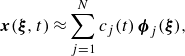 \begin{equation} \boldsymbol {x}(\boldsymbol{\xi },t) \approx \sum _{j=1}^{N} c_j(t)\, \boldsymbol{\phi }_j(\boldsymbol{\xi }), \end{equation}
where $\boldsymbol{\phi }_j(\boldsymbol{\xi })$
is the POD spatial mode,
$\boldsymbol{\phi }_j(\boldsymbol{\xi })$
is the POD spatial mode, $c_j(t)$
is the corresponding temporal coefficient for mode
$c_j(t)$
is the corresponding temporal coefficient for mode $j$
, and
$j$
, and $N$
is the number of modes. Here,
$N$
is the number of modes. Here, $N$
theoretically approaches infinity, but in practice it is taken as the number of snapshots or modes used for reconstruction. In addition, spatial modes are a set of orthogonal modes defined as
$N$
theoretically approaches infinity, but in practice it is taken as the number of snapshots or modes used for reconstruction. In addition, spatial modes are a set of orthogonal modes defined as
 \begin{equation} \int _V \boldsymbol{\phi }_i(\boldsymbol{\xi }) \boldsymbol{\cdot} \boldsymbol{\phi }_j(\boldsymbol{\xi }) \, {\rm d}V = \delta _{ij}, \quad i,j = 1,2,\ldots ,N, \end{equation}
where $V$
is the spatial domain. To compute the POD modes, a set of
$V$
is the spatial domain. To compute the POD modes, a set of $m$
snapshots
$m$
snapshots $\boldsymbol {x}(t_i)=\tilde {\boldsymbol {x}}(\boldsymbol{\xi },t)-\overline {\boldsymbol {x}}(\boldsymbol{\xi })\in \mathbb{R}^n$
is assembled into a snapshot matrix
$\boldsymbol {x}(t_i)=\tilde {\boldsymbol {x}}(\boldsymbol{\xi },t)-\overline {\boldsymbol {x}}(\boldsymbol{\xi })\in \mathbb{R}^n$
is assembled into a snapshot matrix $\boldsymbol {X}=[\boldsymbol {x}(t_1),\boldsymbol {x}(t_2), \ldots ,\boldsymbol {x}(t_m)] \in \mathbb{R}^{n\times m}$
. The covariance matrix is defined as
$\boldsymbol {X}=[\boldsymbol {x}(t_1),\boldsymbol {x}(t_2), \ldots ,\boldsymbol {x}(t_m)] \in \mathbb{R}^{n\times m}$
. The covariance matrix is defined as
 \begin{equation} \boldsymbol {R}=\boldsymbol {X}\boldsymbol {X}^{T} \in \mathbb{R}^{n \times n}. \end{equation}
Due to the high dimensionality of $\boldsymbol{R}$
, the method of snapshots (Sirovich Reference Sirovich1987) is employed by solving the reduced eigenvalue problem. This approach recognises that the non-zero eigenvalues of
$\boldsymbol{R}$
, the method of snapshots (Sirovich Reference Sirovich1987) is employed by solving the reduced eigenvalue problem. This approach recognises that the non-zero eigenvalues of $\boldsymbol {R}=\boldsymbol {X}\boldsymbol {X}^{T}$
are the same as those of the smaller
$\boldsymbol {R}=\boldsymbol {X}\boldsymbol {X}^{T}$
are the same as those of the smaller $\boldsymbol {X}^{T}\boldsymbol {X}\in \mathbb{R}^{m \times m}$
. We therefore solve the eigenvalue problem of size
$\boldsymbol {X}^{T}\boldsymbol {X}\in \mathbb{R}^{m \times m}$
. We therefore solve the eigenvalue problem of size $m$
:
$m$
:
 \begin{equation} \boldsymbol {X}^{T}\boldsymbol {X}\boldsymbol{\psi }_j=\lambda _j\boldsymbol{\psi }_j, \end{equation}
where $\boldsymbol{\psi } \in \mathbb{R}^m$
represents the eigenvector associated with the eigenvalue
$\boldsymbol{\psi } \in \mathbb{R}^m$
represents the eigenvector associated with the eigenvalue $\lambda _j$
in the reduced space. Once this smaller problem is solved, the spatial POD mode is recovered by combining the snapshots using
$\lambda _j$
in the reduced space. Once this smaller problem is solved, the spatial POD mode is recovered by combining the snapshots using $\boldsymbol{\psi }_j$
as weights:
$\boldsymbol{\psi }_j$
as weights:
 \begin{equation} \boldsymbol{\phi }_j=\frac {1}{\sqrt {\lambda _j}}\boldsymbol {X}\boldsymbol{\psi }_j. \end{equation}
This approach is mathematically equivalent to performing a singular value decomposition of $\boldsymbol{X}$
, where singular values
$\boldsymbol{X}$
, where singular values $\sigma _j$
relate to POD energy
$\sigma _j$
relate to POD energy $\lambda _j=\sigma ^2_j$
.
$\lambda _j=\sigma ^2_j$
.
D.2. Cumulative total energy and spatial feature with POD mode
The magnitude of the eigenvalue represents the energy of the POD mode. Thus we can quantify the fraction of energy in the dataset of the $n$
th POD mode as
$n$
th POD mode as
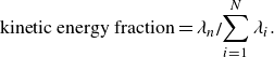 \begin{equation} \text{kinetic energy fraction} = \lambda _n \Bigg/ {\sum _{i=1}^{N} \lambda _i}. \end{equation}
The kinetic energy fraction and normalised cumulative energy results for a supersonic free jet at 10 torr are presented in figure 34. The near-field zone of the 10 torr free jet features shockwaves, making PIV experimental data unavailable. However, from $x/D_{\textit {e}} = 30$
onwards, where shockwaves are absent and self-similarity is satisfied, PIV experimental data align with the MTV data, prompting POD analysis. This analysis aims to unveil turbulent flow structures in the 10 torr free jet. Dominant modes 1–10 encapsulate approximately 20 % of the energy, with mode 1 holding 12 % of the energy, and the turbulent effects are distributed in the subsequent modes.
$x/D_{\textit {e}} = 30$
onwards, where shockwaves are absent and self-similarity is satisfied, PIV experimental data align with the MTV data, prompting POD analysis. This analysis aims to unveil turbulent flow structures in the 10 torr free jet. Dominant modes 1–10 encapsulate approximately 20 % of the energy, with mode 1 holding 12 % of the energy, and the turbulent effects are distributed in the subsequent modes.
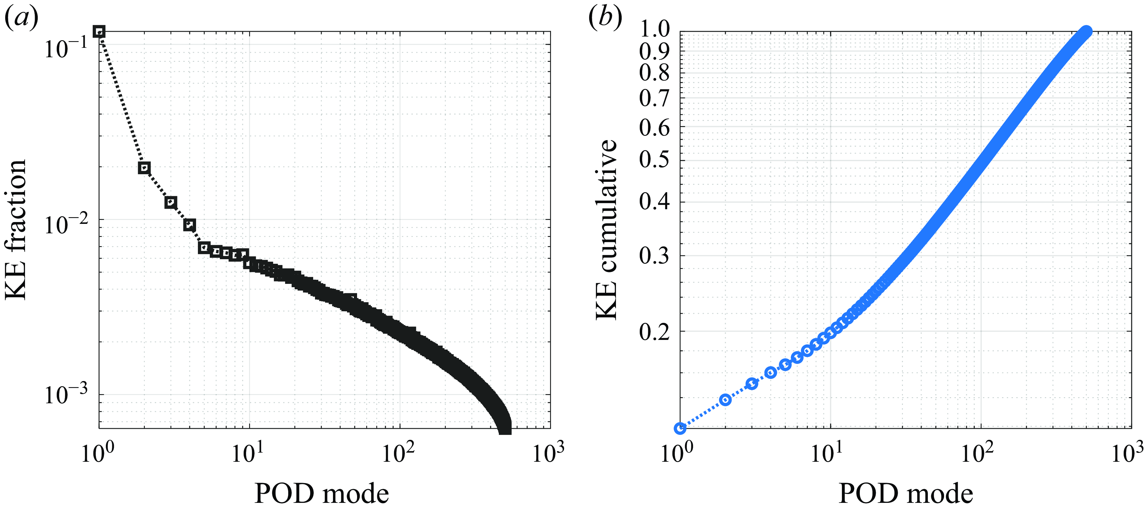
Figure 34. (a) Kinetic energy (KE) fraction and (b) cumulative total energy plot with POD mode at 10 torr (PIV).
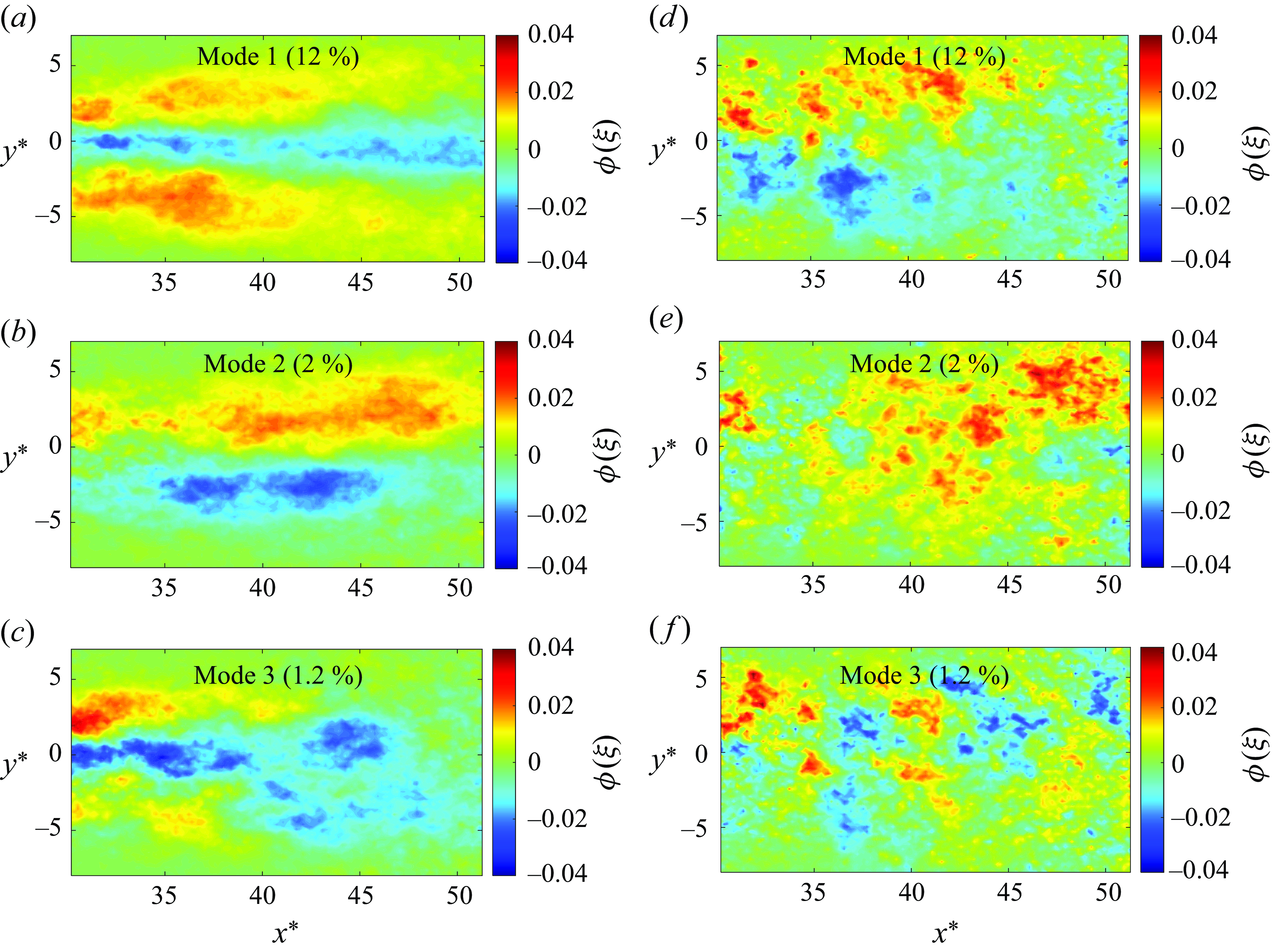
Figure 35. Streamwise eigenfunction contours for (a) mode 1, (b) mode 2, and (c) mode 3. Spanwise eigenfunction contour for (d) mode 1, (e) mode 2, and (f) mode 3.
We examined the eigenfunctions of the dominant modes to understand specific spatial features. Figure 35 depicts the eigenfunctions of the primary modes in the streamwise and spanwise directions, respectively. In modes 1 and 2, the flow exhibits the development of a prominent shear layer, wherein opposing velocity streams converge, leading to the formation of large-scale coherent vortex structures. Conversely, mode 3 is characterised by the shedding of small-scale eddies, which influence flow stability.
The POD analysis of the far-field zone for the 10 torr free jet exhibits turbulent flow structures, providing direct evidence that the flow did not transition back to a stable laminar flow regime.
Appendix E. Comparison between PIV and MTV in an extremely under-expanded supersonic free jet
The findings confirm that MTV adequately measures flow velocities, at least within the near-field zone. To further investigate the difference between MTV and PIV results, the streamwise mean velocity profile is depicted in figure 36. As is evident from figure 36(a), PIV fails to measure the velocity profile at the nozzle exit, due to abrupt density changes. However, the overall shape of the flow profile remains similar. Examining the flow beyond the Mach disk in figure 36(b), MTV results show a sharp velocity decrease in the central region, contrary to the PIV results. As explained for the 10 torr case, the curvature of the Mach disk causes only the central part to act as a normal shockwave, with weaker shocks in surrounding areas. This leads to significant velocity reduction at the centre. Interestingly, while PIV does not capture the velocity decrease induced by the Mach disk, it closely aligns with MTV at the shear layer region surrounding the Mach disk. This implies that the diameter of the Mach disk can be inferred from the distance between the two peaks, which indeed matches closely with theoretical value $D_{{Mach}}/D_e=3.2$
.
$D_{{Mach}}/D_e=3.2$
.
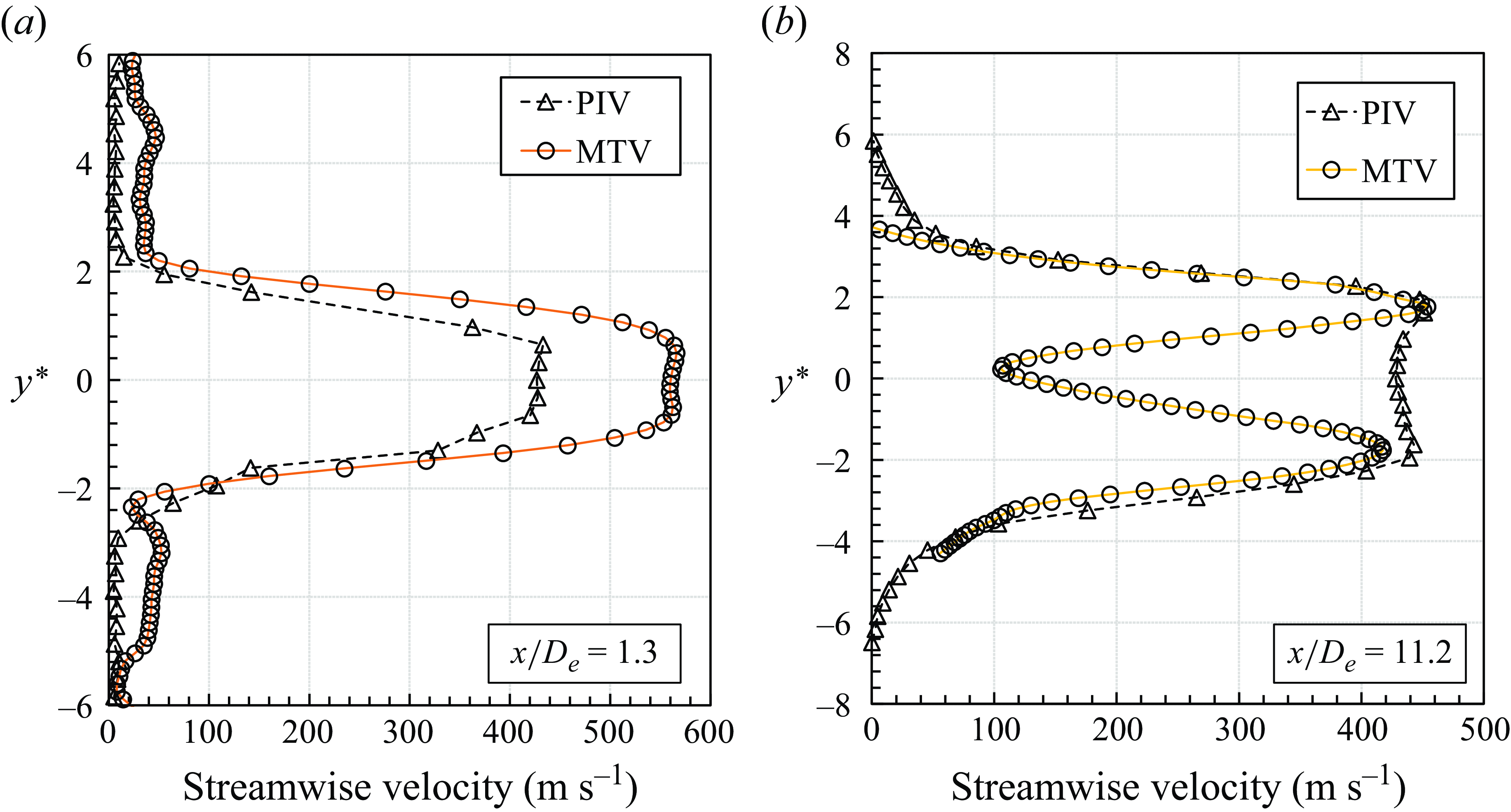
Figure 36. Comparison of streamwise mean velocity profiles in the near-field zone between MTV and PIV at (a) $x/D_{{e}}= 1.3$
and (b)
$x/D_{{e}}= 1.3$
and (b) $x/D_{{e}} = 11.2$
.
$x/D_{{e}} = 11.2$
.
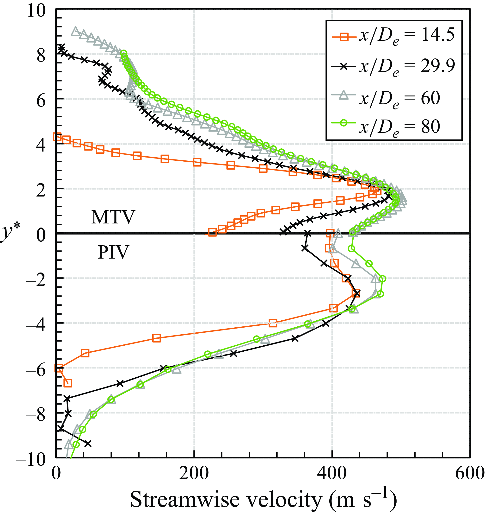
Figure 37. Streamwise mean velocity profile comparison between MTV and PIV in potential core region and far-field zone.
To investigate the development of the mixing layer, we compared MTV and PIV results, which are displayed in figure 37. Both plots show the development of the inner and outer shear layers as they move downstream. However, PIV results do not fully capture the effects induced by the Mach disk, resulting in a slight decrease followed by an increase in the centreline streamwise mean velocity. Additionally, the rate of increase in velocity near the centreline is initially faster in the MTV results, gradually decreasing over distance. This indicates that after the Mach disk, strong shear induced by the velocity gradient leads to a rapid increase in velocity, which then diminishes downstream as the velocity gradient decreases due to the weakening of the shear layer.


 Open access