2.1 Overview of the model

A 3D model of pulse near-field propagation within the compressor was established by Fresnel scalar diffraction theory combined with geometric optics and coordinate transformation. The configuration of the compressor and the coordinates are shown in Figure 1; it is a typical one-pass Treacy configuration^[ Reference Treacy^26], but consists of four identical mosaic gratings. For kilojoule PW lasers, neglecting the STCs^[ Reference Homoelle, Crane, Shverdin, Haefner and Siders^27], the incident field is written as follows:

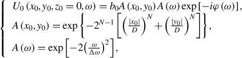(1) $$\begin{align}\left\{\begin{array}{l}{U}_0\left({x}_0,{y}_0,{z}_0=0,\omega \right)={b}_0A\left({x}_0,{y}_0\right)A\left(\omega \right)\exp \left[- i\varphi \left(\omega \right)\right],\\ {}A\left({x}_0,{y}_0\right)=\exp \left\{-{2}^{N-1}\left[{\left(\frac{\mid {x}_0\mid }{D}\right)}^N+{\left(\frac{\mid {y}_0\mid }{D}\right)}^N\right]\right\},\\ {}A\left(\omega \right)=\exp \left[-2{\left(\frac{\omega }{\varDelta \omega}\right)}^2\right],\end{array}\right.\end{align}$$

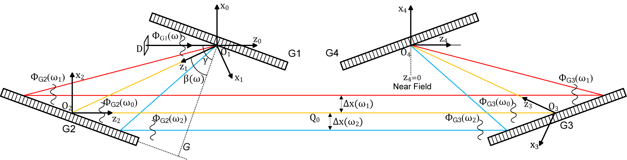
Figure 1 Schematic of the broadband pulse propagation model for grating compressors.

where $D$ is the full width at ${e}^{-2}$ maximum intensity of the super-Gaussian spatial profile, and a plane wave is assumed; $\varDelta \omega$ is the full width at ${e}^{-2}$ maximum intensity of the Gaussian spectral profile; $\varphi \left(\omega \right)$ is the spectral phase; and ${b}_0$ is the energy factor. The incident pulse is diffracted by G1 and divided into multiple sub-beams as different spectral components $\omega$ of beam transmission in different paths, in which $\gamma$ is the incident angle, $\beta \left(\omega \right)$ is the diffraction angle of $\omega$ and the grating law is as follows^[ Reference Bonod and Neauport^28]:

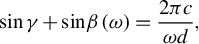(2) $$\begin{align}\sin \gamma +\mathrm{sin}\beta \left(\omega \right)=\frac{2\pi c}{\omega d},\end{align}$$

where $d$ is the grating period. Considering first-order approximation^[ Reference Martinez^29], the diffracted field can be expressed as follows:

(3) $$\begin{align}{U}_1\left({x}_1,{y}_1,0,\omega \right)={A}_{\mathrm{G}1}{b}_1{U}_0\left(\alpha {x}_1,{y}_1,\omega \right)\exp \left(i{\Phi}_{\mathrm{G}1}\right).\end{align}$$

Here the grating is treated as a specialized mirror and its reflection direction is dependent on $\omega$ of the broadband pulse. Further, ${A}_{\mathrm{G}1},{\Phi}_{\mathrm{G}1}$ are the amplitude error and wavefront error introduced by fabrication errors of G1, respectively. ${b}_1$ is the normalized energy factor, 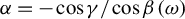$\alpha =-\cos \gamma /\cos \beta \left(\omega \right)$ is the coordinate transformation factor along the dispersion direction, that is, the $x$ direction. It is noted that the diffraction angle of G1 is equal to the incident angle of G2, and similarly for two downstream gratings; the grating law is utilized to trace the center rays of all sub-beams within the compressor, and these center rays are used as the z-axis and baselines for the diffraction propagation of corresponding sub-beams. According to the scalar diffraction theory^[ Reference Goodman^30], the field of $\omega$ on the surface of G2 can be expressed as follows:

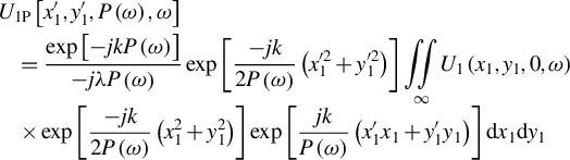(4) $$\begin{align} \begin{array}{@{}l}\displaystyle{U}_{1\mathrm{P}}\left[{x}_1^{\prime},{y}_1^{\prime},P\left(\omega \right),\omega \right]\\[3pt]\displaystyle\quad=\frac{\exp \left[- j k P\left(\omega \right)\right]}{- j\lambda P\left(\omega \right)}\exp \left[\frac{- j k}{2P\left(\omega \right)}\left({x}_1^{\prime 2}+{y}_1^{\prime2}\right)\right]\underset{\infty }{\iint }{U}_1\left({x}_1,{y}_1,0,\omega \right) \\ \displaystyle\quad \times\exp \left[\frac{- j k}{2P\left(\omega \right)}\left({x}_1^2+{y}_1^2\right)\right]\exp \left[\frac{jk}{P\left(\omega \right)}\left({x}_1^{\prime}{x}_1+{y}_1^{\prime}{y}_1\right)\right]\mathrm{d}{x}_1\mathrm{d}{y}_1\end{array}\end{align}$$

where $k=\omega /c$ is the wave number, $G$ is the perpendicular distance between G1 and G2 and $P\left(\omega \right)=G\sec \beta \left(\omega \right)$ is the slant distance for $\omega$ , as illustrated in Figure 1. After that, the field is diffracted by G2 and modulated by ${A}_{\mathrm{G}2},{\Phi}_{\mathrm{G}2}$ , then propagated to G3 and modulated by ${A}_{\mathrm{G}3},{\Phi}_{\mathrm{G}3}$ . Notably, the intersection positions of the G2, G3 surfaces with the center ray of individual sub-beams possess $x\hbox{-} \mathrm{axis}$ shifts due to angular dispersion. Since the sub-beams only illuminate a portion of the grating, the wavefront of each sub-beam is a segment of the overall diffracted wavefront and the $x\hbox{-} \mathrm{axis}$ shifts can be described as the interval between the center rays of $\omega$ and ${\omega}_0$ within G2–G3^[ Reference Li, Tsubakimoto, Yoshida, Nakata and Miyanaga^17]:

(5) $$\begin{align}\varDelta x\left(\omega \right)=G\left[\tan \beta \left(\omega \right)-\tan \beta \left({\omega}_0\right)\right]\cos \gamma.\end{align}$$

With this parameter, the optical pathlength within G2–G3 for $\omega$ can be expressed as follows:

(6) $$\begin{align}Q\left(\omega \right)={Q}_0+2\Delta x\left(\omega \right)\tan \gamma,\end{align}$$

where ${Q}_0$ is the distance between G2 and G3 for ${\omega}_0$ . Finally, the field is transmitted from G3 to G4, which is the reverse process of that for the G1–G2 grating pair. The near-field distribution ${U}_{4 \mathrm{NF}}\left({x}_4,{y}_4,0,\omega \right)$ at G4 is obtained, and the laser fluence can be expressed as follows:

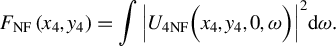(7) $$\begin{align}{F}_{\mathrm{NF}}\left({x}_4,{y}_4\right)=\int {\left|{U}_{4 \mathrm{NF}}\Big({x}_4,{y}_4,0,\omega \Big)\right|}^2\mathrm{d}\omega.\end{align}$$

The spatio-temporal distribution at G4 can be obtained by the inverse Fourier transform of ${U}_{4 \mathrm{NF}}\left({x}_4,{y}_4,0,\omega \right)$ :

(8) $$\begin{align}{U}_{4 \mathrm{NF}}\left({x}_4,{y}_4,0,t\right)=\frac{1}{2\pi}\underset{-\infty }{\overset{+\infty }{\int }}{U}_{4 \mathrm{NF}}\left({x}_4,{y}_4,0,\omega \right)\exp \left( i\omega t\right)\mathrm{d}\omega.\end{align}$$

In general, the propagation model described above can calculate the spatio-spectral distribution at any position within the compressor by establishing a unified coordinate and undergoing coordinate rotation. This study primarily focuses on near-field modulation at G4 induced by errors of the upstream grating to investigate control requirements of these errors as G4 suffers the greatest risk of laser-induced damage.

2.2 Periodic wavefront error

For holographic gratings, the diffracted wavefront errors are originated from groove errors caused by an imperfect exposure system and surface imperfection^[ Reference Khazanov^31], and the periodic wavefront errors are introduced during the fabrication process^[ Reference Shi, Zeng and Li^7], for example, small-tool polishing of the substrate and exposure system imperfection. The two-dimensional (2D) periodic wavefront error can be expressed as follows^[ Reference Li and Miyanaga^32]:

(9) $$\begin{align}\Phi \left(x,y,\omega \right)=k\frac{H}{2}\left[\frac{\sin \left(2\pi \frac{x}{T}\right)+\sin \left(2\pi \frac{y}{T}\right)}{2}\right],\end{align}$$

where $H$ is the peak-to-valley (PV) value of the wavefront error and $T$ is the spatial period. The periods in two directions are assumed to be equal and the variation of PV value with $\omega$ is neglected for the narrowband laser pulse. Utilizing the parameter in Equation (5), the wavefront error can be described as ${\Phi}_{\mathrm{G}1}\left({x}_1,{y}_1,\omega \right)$ with an arbitrary frequency $\omega$ for G1, but ${\Phi}_{\mathrm{G}2}\left({x}_2-\varDelta x\left(\omega \right),{y}_2,\omega \right)$ for G2 and ${\Phi}_{\mathrm{G}3}\left({x}_3-\frac{\varDelta x\left(\omega \right)}{\alpha },{y}_3,\omega \right)$ for G3.

2.3 Mosaic gap error

As mentioned above, the mosaic gap error is an inherent limitation of grating mosaic techniques, including amplitude error and phase jump. The amplitude error not only degrades the temporal contrast of the pulse^[ Reference Trentelman, Ross and Danson^33, Reference Mikhail, Alexander and Horst^34] but also causes near-field modulation by hard edge diffraction. The SG-II UP PW picosecond system compressor utilizes a $1.4\;\mathrm{m}\times 0.42\;\mathrm{m}$ grating with two mosaic gaps located along one-third and two-thirds of its length; the amplitude error function for these gaps is given by the following:

(10) $$\begin{align}&A\left(x,y,\omega \right)\nonumber\\&\quad =1-\left\{ \mathrm{rect}\left[\frac{x+\frac{L}{6}\cos \beta \left(\omega \right)}{{w}\cos \beta \left(\omega \right)}\right]+ \mathrm{rect}\left[\frac{x-\frac{L}{6}\cos \beta \left(\omega \right)}{{w}\cos \beta \left(\omega \right)}\right]\right\},\end{align}$$

where ${w}$ represents the gap width, $L$ denotes the grating length and ${w}\cos \beta \left(\omega \right)$ is the corresponding gap width on the diffracted beam plane. Besides, the diffraction angle at G2 is $\gamma$ , so the corresponding gap width is ${w}\cos \gamma$ . Similar to the wavefront error, the amplitude error function for G1 is ${A}_{\mathrm{G}1}\left({x}_1,{y}_1,\omega \right)$ , while for G2 and G3 they are ${A}_{\mathrm{G}2}\left({x}_2-\varDelta x\left(\omega \right),{y}_2,\omega \right)$ and ${A}_{\mathrm{G}3}\left({x}_3-\frac{\varDelta x\left(\omega \right)}{\alpha },{y}_3,\omega \right)$ , respectively. Moreover, the gap-induced wavefront errors such as phase jump are dependent on the grating fabrication process, and their impacts are assessed through two wavefronts measured by an interferometer.

3.1 Simulation parameters

The near-field fluence modulation index, defined as the maximum value of the fluence profile divided by its average value^[ Reference Li, Du, Wu, Ding, Lu, Wang, An and Cui^35], is adopted to evaluate the impact of two types of errors on the near field at G4 (hereafter referred to as NF4). Based on the status of the SG-II UP PW picosecond system, the simulated pulse possesses a center wavelength of $1053\;\mathrm{nm}$ and a bandwidth (full width at half maximum (FWHM)) of $3.8\;\mathrm{nm}$ . The input beam of the compressor is 10th-order super-Gaussian with a zero-intensity area (at $1\%$ maximum intensity) of $320\;{\mathrm{mm}}\times 320\;{\mathrm{mm}}$ , and the energy of the output pulse duration is $1.2\;\mathrm{kJ}@10\;\mathrm{ps}$ . The spectral sampling window is set as 18 nm centered at 1053 nm, and the spatial sampling windows are $380\; \mathrm{mm}\times 380\; \mathrm{mm}$ . The sampling points are $4096,4096,512\left(x,y,\lambda \right)$ for fluence calculation, and $512,512,512\left(x,y,\lambda \right)$ for laser peak power calculation. The groove density of the grating is $1740\;\mathrm{gr}/\mathrm{mm}$ , the incident angle is ${71}^{\circ}$ , the perpendicular distance $G$ of each grating pair is $2146\;\mathrm{mm}$ and the optical pathlength between G2 and G3 for ${\omega}_0$ is $10,617\;\mathrm{mm}$ . To facilitate analysis, the near-field modulation index of the input pulse is set to 1, representing an ideal case, and the input energy is assumed to be $1.2\;\mathrm{kJ}$ .

3.2 NF4 fluence modulation induced by periodic wavefront errors

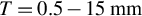
Figure 2 shows the 2D NF4 fluence modulation induced by the 2D periodic wavefront error of G1 with $T=15\;\mathrm{mm}, H=\lambda /4$ . It can be observed that the periodic wavefront error results in periodic NF4 fluence modulation. The maximum modulation index has reached about $1.55$ ; this phenomenon is known as the Talbot effect^[ Reference Koch, Lehr and Glaser^23], and it results in similar distributions of NF4 fluence and the accumulation of ${\Phi}_{\mathrm{G}1}$ over $\omega$ . The periods of wavefront errors in the two directions are assumed to be identical, but the diffracted beam broadens along the $x$ direction due to $\beta \left(\omega \right)<\gamma <{90}^{\circ }$ , which represents that the periods of wavefront vary with $\omega$ after diffraction, but this variation is compensated at NF4. In other words, the diffracted wavefront can be equivalent to the input wavefront for G1, and the input wavefront is directly mapped to the distribution of NF4 fluence.

Figure 2 NF4 fluence modulation induced by the periodic wavefront error ${\Phi}_{\mathrm{G}1}$ with $T=15\;\mathrm{mm}$ , $H=\lambda /4$ . (a) Accumulation of ${\Phi}_{\mathrm{G}1}$ over $\omega$ at the input beam plane. (b) NF4 fluence modulation induced by ${\Phi}_{\mathrm{G}1}$ .

The NF4 fluence modulations caused by ${\Phi}_{\mathrm{G}2}$ or ${\Phi}_{\mathrm{G}3}$ with $T=15\;\mathrm{mm},\ H=\lambda /4$ are displayed in Figure 3. As described in Section 2, ${\Phi}_{\mathrm{G}2}$ and ${\Phi}_{\mathrm{G}3}$ possess $\omega$ -dependent shift along the dispersion direction, which indicates that the initial phase of periodic wavefront for individual sub-beams varies with $\omega$ . To evaluate the effects of wavefront errors on NF4 fluence, ${\Phi}_{\mathrm{G}2}$ and ${\Phi}_{\mathrm{G}3}$ of each sub-beam are accumulated over $\omega$ in the same aperture as the sub-beams are recombined at NF4. The summed result of the wavefronts is smoothed along the $x$ direction due to the different initial phases. As a result, the fluence modulation is smoothed along the $x$ direction, which can be seen in Figures 3(b) and 3(d). It is important to note that the accumulations of wavefront errors are fictitious distributions without physical significance, but they provide representations of the induced fluence modulation characteristics.

Figure 3 NF4 fluence modulation induced by the periodic wavefront errors ${\Phi}_{\mathrm{G}2}$ or ${\Phi}_{\mathrm{G}3}$ with $T=15\;\mathrm{mm},H=\lambda /4$ . (a) Accumulation of ${\Phi}_{\mathrm{G}2}$ over $\omega$ in the same aperture. (b) NF4 fluence modulation induced by ${\Phi}_{\mathrm{G}2}$ . (c) Accumulation of ${\Phi}_{\mathrm{G}3}$ over $\omega$ in the same aperture. (d) NF4 fluence modulation induced by ${\Phi}_{\mathrm{G}3}$ .

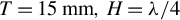
Figure 4 exhibits the NF4 intensity distributions induced by ${\Phi}_{\mathrm{G}2}$ in different spectral components, in which the distortions of the intensity arise from spectral clipping of the compressor. It can be seen that the intensity modulation of each sub-beam is similar to the distribution of ${\Phi}_{\mathrm{G}2}$ , which is a feature of the Talbot effect; the different initial phases of ${\Phi}_{\mathrm{G}2}$ result in different intensity distributions. Ultimately, the fluence modulations are smoothed along the dispersion direction. This interesting property can significantly mitigate fluence modulation induced by ${\Phi}_{\mathrm{G}2}$ and ${\Phi}_{\mathrm{G}3}$ ; in the case of $T=15\;\mathrm{mm},H=\lambda /4$ , the modulation index is only about $1.2$ for ${\Phi}_{\mathrm{G}2}$ and $1.05$ for ${\Phi}_{\mathrm{G}3}$ , much less than 1.7 for ${\Phi}_{\mathrm{G}1}$ . In addition, it can be observed that the NF4 peak fluence caused by ${\Phi}_{\mathrm{G}2}$ is higher than that caused by ${\Phi}_{\mathrm{G}3}$ . It is evident that an increased propagation distance can exacerbate the NF4 fluence modulation induced by wavefront errors under present working distances.

Figure 4 (a) The distributions of ${\Phi}_{\mathrm{G}2}$ along the ${x}_2$ direction with ${y}_2=0$ for different wavelengths; the black line represents the accumulated result of ${\Phi}_{\mathrm{G}2}$ . (b) The resulting NF4 intensity distribution at different wavelengths along the ${x}_4$ direction with ${y}_4=0$ ; the fluence along the ${x}_4$ direction is displayed at the bottom.

To study the effects of different PV values and periods of periodic wavefront errors for the first three gratings on NF4, considering a period range of $0.5-40\;\mathrm{mm}$ with an interval of $0.5\;\mathrm{mm}$ , $T=0$ corresponds to the ideal case. The NF4 fluence modulations induced by single-period wavefront errors with PV value of $\lambda /4\;\mathrm{or}\;\lambda /8$ for each upstream grating are calculated, as shown in Figures 5(a)–5(c), and for all three gratings, as shown in Figure 5(d). It can be seen that the modulation index is roughly proportional to the square of the PV value, which is consistent with the analysis in Ref. [Reference Zhou and Burge36]. Under the fixed optical distance to G4, for three upstream gratings, the mid-to-high spatial frequency wavefront errors lead to oscillatory distributions of modulation index, and the peak modulation index is only induced by wavefront errors of characteristic periods, which is also a feature of the Talbot effect. On the other hand, the characteristic periods are distinct for each grating due to different propagation distance of the fields: for ${\Phi}_{\mathrm{G}1}$ , they are 3.5 and 5–7 mm with the maximum modulation index exceeding 3. For ${\Phi}_{\mathrm{G}2}$ , they are 2, 3, 4.5 and 6 mm, with the maximum modulation index of about 1.78. For ${\Phi}_{\mathrm{G}3}$ , they are 1, 2 and 2.5 mm, with the maximum modulation index of about 1.78, and they are 2.5 and 4.5–11 mm with the maximum modulation index exceeding 3 for all. In addition, to limit the modulation index to less than $1.5$ , in the case of $H=\lambda /4$ , the period ranges that need to be controlled are $0.5-15\;\mathrm{mm}$ for ${\Phi}_{\mathrm{G}1}$ , $0.5-10\;\mathrm{mm}$ for ${\Phi}_{\mathrm{G}2}$ , $0.5-5\;\mathrm{mm}$ for ${\Phi}_{\mathrm{G}3}$ and $0.5-20\;\mathrm{mm}$ for all. In the case of $H=\lambda /8$ , the ranges are $0.5-12\;\mathrm{mm}$ for ${\Phi}_{\mathrm{G}1}$ and $0.5-15\;\mathrm{mm}$ for all three gratings; for only ${\Phi}_{\mathrm{G}2}$ or ${\Phi}_{\mathrm{G}3}$ , all the induced modulation indices are less than 1.5. It needs to be emphasized that these ranges are obtained based on the wavefront errors of the diffracted beam, which must be divided by $\cos {\beta}_0$ for ${\Phi}_{\mathrm{G}1}$ , ${\Phi}_{\mathrm{G}3}$ or $\cos \gamma$ for ${\Phi}_{\mathrm{G}2}$ to be approximately transformed onto the grating plane.

Figure 5 NF4 fluence modulation induced by (a) ${\Phi}_{\mathrm{G}1}$ , (b) ${\Phi}_{\mathrm{G}2}$ , (c) ${\Phi}_{\mathrm{G}3}$ and (d) periodic wavefront errors of all upstream gratings, with $T=0.5-40\;\mathrm{mm},\; H=\lambda /4\;\mathrm{or}\;\lambda /8$ .

In general, the maximum modulation index induced by the periodic wavefront errors of G2 and G3 is significantly lower than that of G1; G1 also possesses the maximum characteristic period, confirming the influence of angular dispersion and diffraction effects described previously. Besides, the result in Figure 5(d) reveals a significant enhancement of NF4 fluence modulation at the overlapping characteristic periods of each grating. It is worth noting that the simulation considers only single-period wavefront errors to evaluate the characteristic period ranges for NF4. However, actual fabrication typically produces wavefronts with multiple periods. Calculations based on the measured wavefronts presented in Section 3.4 suggest a better performance of the practical multiple-period wavefront errors.

3.3 NF4 fluence modulation induced by mosaic gap amplitude error

In the gap area of the mosaic grating no exposure takes place, leading to energy loss of the diffracted beam, defined as gap amplitude error. Figure 6(a) illustrates the gap amplitude error on the diffracted beam plane at G1, as described in Section 2.3. The spatial positions of the mosaic gaps are independent of $\omega$ , but the equivalent gap width varies with $\omega$ . The resulting NF4 fluence modulation is shown in Figure 6(b), with a modulation index of $1.7$ ; intense modulation is originated from the diffraction effects of the gap edges. The output energy is reduced to $1.178\;\mathrm{kJ}$ , the laser peak power is decreased by approximately $1.2\%$ from $1.127\times {10}^{14}$ to $1.113\times {10}^{14}\;\mathrm{W}$ ; this result remains valid for the G2 and G3 gap amplitude error. Notably, the modulations induced by the two gaps are independent of each other and exhibit a pattern akin to a thin opaque strip^[ Reference Wichtowski^37].

Figure 6 NF4 fluence modulation induced by gap amplitude error ${A}_{\mathrm{G}1}$ . (a) Diagram of gap amplitude error for three selected frequencies on the diffracted beam plane at G1. (b) NF4 fluence modulation induced by ${A}_{\mathrm{G}1}$ .

The amplitude errors of the diffracted beam caused by the gaps on the grating planes at G2 and G3 are displayed in Figures 7(a) and 7(c), respectively. Similarly, the spatial positions of gap amplitude error for each sub-beam are dependent upon $\omega$ at G2 and G3 due to angular dispersion. As $\omega$ increases, the gap positions shift from right to left on the diffracted beam plane at G2, and shift in the opposite direction at G3, as marked by the red lines in the Figure 6. Ultimately, the NF4 fluence modulations induced by the gap amplitude error of these two gratings are smoothed due to the sweep of gap positions, with two tiny depressions forming at the location of gaps. The modulation indices in the two cases are almost identical, both about 1.04.

Figure 7 NF4 fluence modulation induced by gap amplitude errors ${A}_{\mathrm{G}2}$ and ${A}_{\mathrm{G}3}$ . (a) Diagram of gap amplitude error for three selected frequencies on the diffracted beam plane at G2. (b) NF4 fluence modulation induced by ${A}_{\mathrm{G}2}$ . (c) Diagram of gap amplitude error for three selected frequencies on the diffracted beam plane at G3. (d) NF4 fluence modulation induced by ${A}_{\mathrm{G}3}$ .

Figure 7 demonstrates that the gap amplitude errors of G2 and G3 have a relatively minor impact on NF4 compared to that of G1. Therefore, the further analysis is only focused on G1. Considering a gap width range of ${w}=0.5-6\;\mathrm{mm}$ with an interval of $0.5\;\mathrm{mm}$ on the grating plane; the equivalent width on the diffracted beam plane of G1 is $w\text{cos}\beta(\omega)$ . The modulation index is calculated and shown with a blue line in Figure 8(a). The other curves in Figure 8(a) represent modulations induced by thin strip diffraction with three fixed strip widths of $w\mathrm{cos}{\beta}_0,{w}/2.6\;\mathrm{and}\;{w}/2.8$ on the beam plane under a propagation distance of $20\;\mathrm{m}$ for ${\omega}_0$ , which is equal to the working distance of ${Q}_0=10,617\;\mathrm{mm}$ . The results reveal that the NF4 fluence modulation characteristics caused by ${A}_{\mathrm{G}1}$ closely resemble those induced by thin strip diffraction. Due to the $\omega$ -dependent equivalent width, the characteristics of NF4 fluence modulation align more closely with the thin strip diffraction with widths of ${w}/2.6,{w}/2.8$ , instead of a strip width of ${w}\cos {\beta}_0$ ( ${w}/2.2$ , approximately). Within the range of ${w}=0.5-6\;\mathrm{mm}$ , smaller widths result in lower NF4 fluence modulation, but the width of the mosaic gap is limited to $3-5\;\mathrm{mm}$ under the current fabrication conditions. Therefore, considering the typical cases of ${{w}=3\kern0.24em \mathrm{or}\;5\;\mathrm{mm}}$ , the fluence modulation is induced by ${A}_{\mathrm{G}1}$ with ${Q}_0=10,617\hbox{--} 14,717\;\mathrm{mm}$ , about $20\hbox{--} 24\;\mathrm{m}$ optical pathlength for ${\omega}_0$ , and the modulations induced by thin strip diffraction with widths of ${w}/2.6,{w}/2.8$ under the propagation distances between 20 and 24 m are shown in Figure 8(b). It can be observed that changing the working distance cannot significantly mitigate the NF4 fluence modulation induced by ${A}_{\mathrm{G}1}$ ; when ${Q}_0$ is lengthened by 4 m, the modulation index only decreases by about $3\%$ .

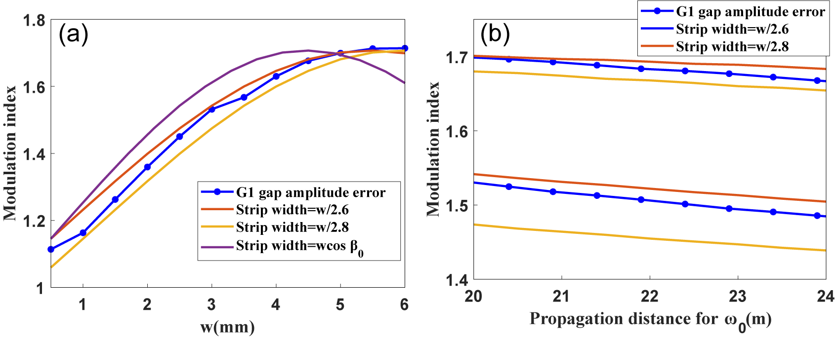
Figure 8 Comparison of the modulation index induced by diffraction of the G1 mosaic gap and thin strip. (a) NF4 fluence modulation induced by ${A}_{\mathrm{G}1}$ and the modulation induced by strip diffraction for ${\omega}_0$ under different ${w}$ ; the propagation distance is $20\;\mathrm{m}$ . (b) The variation of the modulations with the propagation distance (upper, ${w}=5\;\mathrm{mm}$ ; lower, ${w}=3\;\mathrm{mm}$ ).

3.4 NF4 fluence modulation induced by the measured wavefront of the mosaic grating

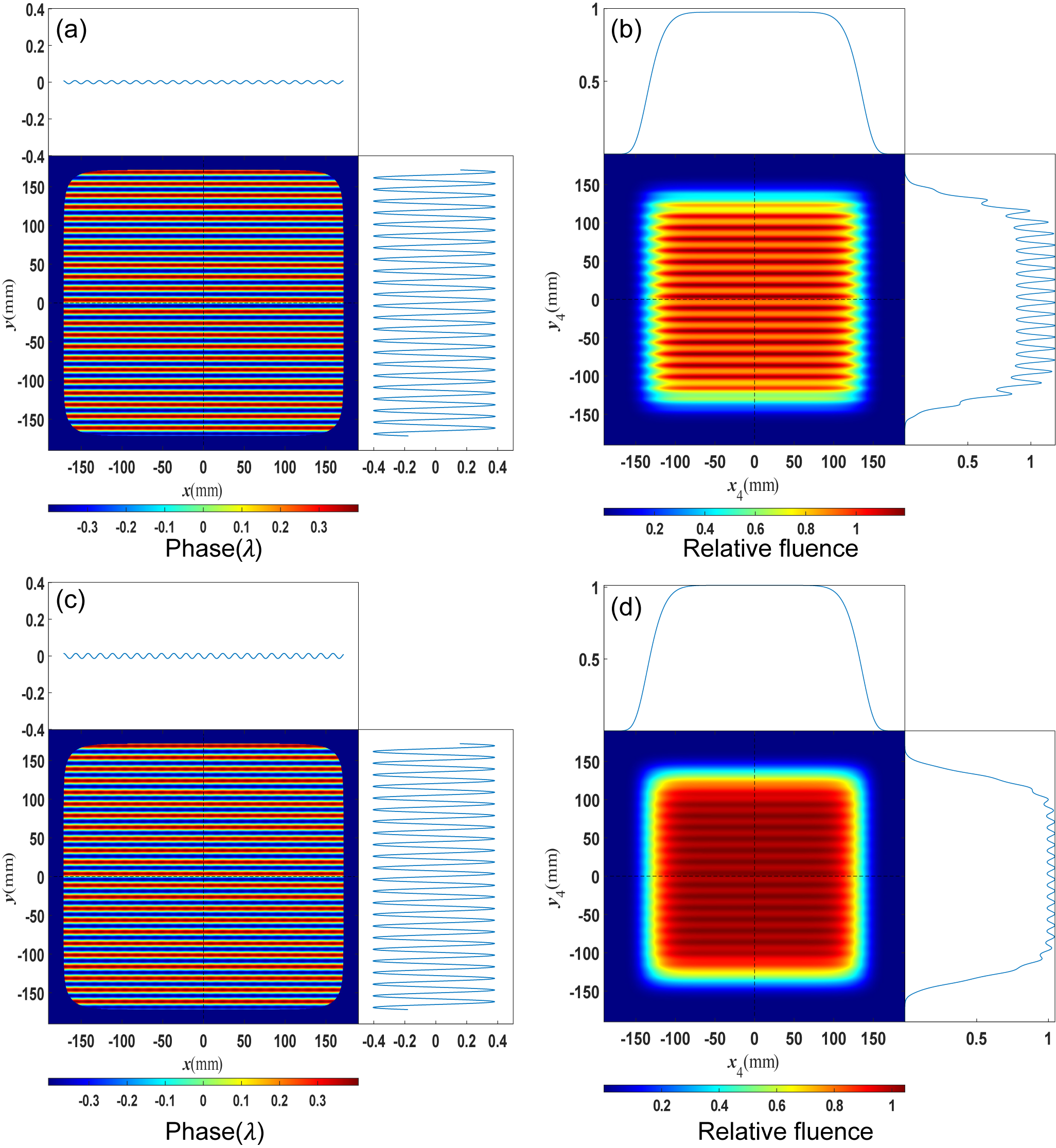
To evaluate the characteristics of NF4 fluence modulation caused by phase jump across the mosaic gap, two diffracted wavefronts with phase jumps across $5\;\mathrm{mm}$ width gaps are introduced, which are shown in Figures 9(a) and 9(b). The gratings are Littrow mounted, the monochromatic probe light with $\lambda =1053\;\mathrm{nm}$ is diffracted to propagate along the incident path and returns to the interferometer and the four corners of measured wavefront distribution are cropped due to the interferometer possessing a circular aperture with $600\;\mathrm{mm}$ diameter. It can be observed that the phase jump of the first wavefront is more severe, and there are mid-to-high-frequency wavefront errors at the mosaic gaps. For the $1.4\;\mathrm{m}\times 0.42\;\mathrm{m}$ grating utilized in the SG-II UP PW picosecond system compressor, the Littrow angle is ${66}^{\circ }$ , the length of the rectangle in lateral view is about $569\;\mathrm{mm}$ and the resolution is $0.274\;\mathrm{mm}$ with $1500\times 2050$ sampling points for two wavefronts, respectively.

Figure 9 Two diffracted wavefronts from Littrow-mounted mosaic gratings measured by a $600\;\mathrm{mm}$ circular-aperture interferometer. (a) The first wavefront with a PV value of about $0.3\lambda$ . (b) The second wavefront with a PV value of about $0.9\lambda$ .

Based on the previous results, we only consider the G1 errors with the most severe impact on the NF4 in this section. The area enclosed by black dotted lines in Figure 9 corresponds to the aperture of the input beam and the interpolation algorithm is adopted to increase the sampling points to $4096\times 4096$ , taking the two wavefronts as ${\Phi}_{\mathrm{G}1}$ . The resulting NF4 fluence modulations are shown in Figures 10(a) and 10(c), respectively. It is obvious that the peak fluence modulation is induced by mid-to-high-frequency wavefront error across the mosaic gap, and both of the fluence modulation indices reach approximately 1.36, implying that the low-frequency wavefront error has almost no effect on NF4. After introducing the amplitude error ${A}_{\mathrm{G}1}$ , the near-field modulations are deteriorated as displayed in Figures 10(b) and 10(d). It can be seen that the combined effect of wavefront and amplitude errors further degrades the near-field quality, with the near-field modulation index reaching 1.9 for the first wavefront and 1.8 for the second. Notably, the first wavefront, which has a smaller PV value, results in a higher modulation index than the second wavefront; this phenomenon is caused by the worse continuity across the gap of the first wavefront. Furthermore, referring to Figures 6–8 and 10, it is evident that the near-field modulation induced by the G1 gap amplitude error is dominant under the current status, confirming that controlling the mosaic gap width of G1 is an effective approach to mitigate near-field modulation.

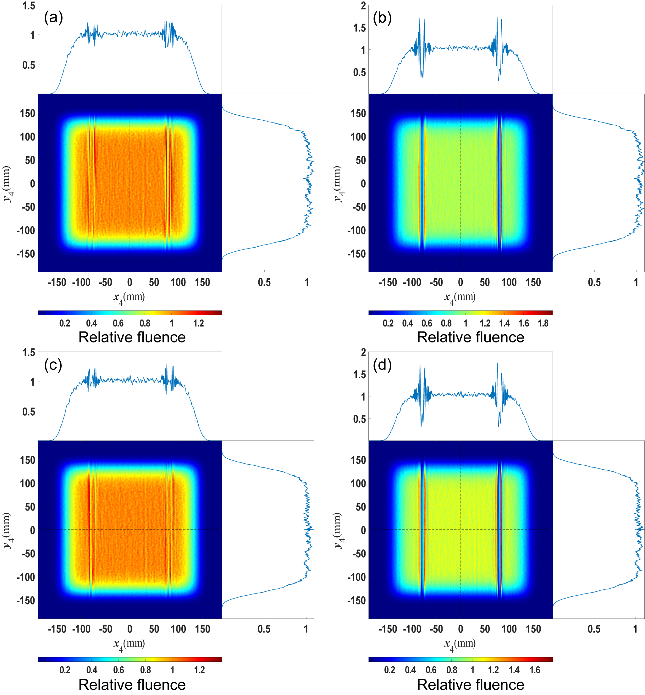
Figure 10 NF4 fluence modulation induced by (a) the first wavefront without ${A}_{\mathrm{G}1}$ , (b) both the first wavefront and ${A}_{\mathrm{G}1}$ , (c) the second wavefront without ${A}_{\mathrm{G}1}$ and (d) both the second wavefront and ${A}_{\mathrm{G}1}$ .