


1 Introduction
For many years, substantial efforts have been made to study laser–matter interactions and to produce sources of secondary radiations such as energetic ions. The introduction of chirped pulse amplification (CPA) has significantly increased the achievable intensities of the laser systems[
Reference Strickland and Mourou1] and contemporary laser facilities are capable of achieving intensities[
Reference Bahk, Rousseau, Planchon, Chvykov, Kalintchenko, Maksimchuk, Mourou and Yanovsky2] at the laser focus of up to ${10}^{22}\ \mathrm{W}/{\mathrm{cm}}^2$
. During the interaction of such an intense laser pulse with a target, the intensity in its rising edge and/or ASE (amplified spontaneous emission) is powerful enough to convert the material into a plasma. Consequently, the main part of the pulse interacts with a highly ionized and heated plasma, which results in particle acceleration of electrons and ions.
${10}^{22}\ \mathrm{W}/{\mathrm{cm}}^2$
. During the interaction of such an intense laser pulse with a target, the intensity in its rising edge and/or ASE (amplified spontaneous emission) is powerful enough to convert the material into a plasma. Consequently, the main part of the pulse interacts with a highly ionized and heated plasma, which results in particle acceleration of electrons and ions.
However, using solid targets necessitates precise alignment for each shot and results in debris generation and deposition on nearby high-intensity laser optics. This makes it challenging to use in new high-repetition-rate (around 10 Hz and with kHz expected), ultra-high-intensity laser (sources of more intense electromagnetic pulses (EMPs)) facilities, such as Apollon[ Reference Papadopoulos, Zou, Le Blanc, Cheriaux, Georges, Druon, Mennerat, Martin, Freneaux, Beluze, Lebas, Monot, Mathieu and Audebert3], ELI[ Reference Margarone, Cirrone, Cuttone, Amico, Andò, Borghesi, Bulanov, Bulanov, Chatain, Fajstavr, Giuffrida, Grepl, Kar, Krasa, Kramer, Larosa, Leanza, Levato, Maggiore, Manti, Milluzzo, Odlozilik, Olsovcova, Perin, Pipek, Psikal, Petringa, Ridky, Romano, Rus, Russo, Schillaci, Scuderi, Velyhan, Versaci, Wiste, Zakova and Korn4, Reference Radier, Chalus, Charbonneau, Thambirajah, Deschamps, David, Barbe, Etter, Matras, Ricaud, Leroux, Richard, Lureau, Baleanu, Banici, Gradinariu, Caldararu, Capiteanu, Naziru, Diaconescu, Iancu, Dabu, Ursescu, Dancus, Ur, Tanaka and Zamfir5] or VEGA[ Reference Huault, Zeraouli, Ajates, Apiñaniz, García, Hernández-Palmero, Malko, Mendez, Perez-Hernández, Pisonero, Salgado-Lopez, Vaisseau, Varela, Gatti, Volpe, Roso, Fedosejevs, Longman, Shepherd and Hill6]. To address these challenges, researchers are exploring self-regenerating targets, including water jets[ Reference George, Morrison, Feister, Ngirmang, Smith, Klim, Snyder, Austin, Erbsen, Frische, Nees, Orban, Chowdhury and Roquemore7, Reference Puyuelo-Valdes, de Luis, Hernandez, Apiñaniz, Curcio, Henares, Huault, Perez-Hernández, Roso, Gatti and Volpe8] or droplets[ Reference Karsch, Düsterer, Schwoerer, Ewald, Habs, Hegelich, Pretzler, Pukhov, Witte and Sauerbrey9, Reference Ter-Avetisyan, Schnürer, Nickles, Smirnov, Sandner, Andreev, Platonov, Psikal and Tikhonchuk10], cryogenic ribbons[ Reference Margarone, Velyhan, Dostal, Ullschmied, Perin, Chatain, Garcia, Bonnay, Pisarczyk, Dudzak, Rosinski, Krasa, Giuffrida, Prokupek, Scuderi, Psikal, Kucharik, De Marco, Cikhardt, Krousky, Kalinowska, Chodukowski, Cirrone and Korn11], tape targets[ Reference Ehret, de Luis, Apiñaniz, Henares, Lera, Perez-Hernández, Puyuelo-Valdes, Volpe and Gatti12] and liquid crystal films[ Reference Thoss13, Reference Poole, Andereck, Schumacher, Daskalova, Feister, George, Willis, Akli and Chowdhury14]. In addition, near-critical density targets such as high-density gas jets are being investigated[ Reference Palmer, Dover, Pogorelsky, Babzien, Dudnikova, Ispiriyan, Polyanskiy, Schreiber, Shkolnikov, Yakimenko and Najmudin15– Reference Henares, Puyuelo-Valdes, Hannachi, Ceccotti, Ehret, Gobet, Lancia, Marques, Santos, Versteegen and Tarisien17].
Diagnosing and characterizing the spectra of individual ion species is crucial for understanding the fundamental acceleration mechanisms, which range from target normal sheath acceleration (TNSA)[ Reference Burdonov, Fazzini, Lelasseux, Albrecht, Antici, Ayoul, Beluze, Cavanna, Ceccotti, Chabanis, Chaleil, Chen, Chen, Consoli, Cuciuc, Davoine, Delaneau, D’humières, Dubois, Evrard, Filippov, Freneaux, Forestier-Colleoni, Gremillet, Horny, Lancia, Lecherbourg, Lebas, Leblanc, Ma, Martin, Negoita, Paillard, Papadopoulos, Perez, Pikuz, Qi, Quéré, Ranc, Söderström, Scisciò, Sun, Vallières, Wang, Yao, Mathieu, Audebert and Fuchs18] to radiation pressure acceleration (RPA)[ Reference Esirkepov, Borghesi, Bulanov, Mourou and Tajima19] and magnetic vortex acceleration[ Reference Nakamura, Bulanov, Esirkepov and Kando20] or collisionless shock acceleration (CSA)[ Reference Bonvalet, Loiseau, Marques, Atukpor, d’Humieres, Domange, Forestier-Colleoni, Hannachi, Lancia, Raffestin, Tarisien, Tikhonchuk and Nicolaï21], depending on the target. At high repetition rates, the time-of-flight (TOF) method based on a stacked diamond detector structure can be used to measure the velocity of the accelerated particles[ Reference Salvadori, Consoli, Verona, Cipriani, Anania, Andreoli, Antici, Bisesto, Costa, Cristofari, De Angelis, Giorgio, Ferrario, Galletti, Giulietti, Migliorati, Pompili and Zigler22]. However, it is not possible with this method to determine the type of particles detected. In addition, this diagnosis is not necessarily ideal given its experimental footprint. Of the diagnostic tools frequently employed in single-shot pulses – such as radiochromic film stack detectors[ Reference Curry, Dunning, Gauthier, Chou, Fiuza, Glenn, Tsui, Bazalova-Carter and Glenzer23] or nuclear activation methods[ Reference Tarisien, Gobet, Hannachi, Aléonard, Claverie, Gerbaux, Malka, Scheurer, Méot, Morel, Audebert, Brambrink, Nicolai, Tikhonchuk and Amthor24] – Thomson parabola (TP) spectrometers stand out. They provide the ability to separate different ion species by the energy and mass-to-charge ratio (A/Z) using static electric and magnetic fields.
A significant drawback of traditional TP spectrometers is their dependence on localization detection system, such as imaging plates (IPs) and Columbia Resin #39 (CR-39)[ Reference Cobble, Flippo, Offermann, Lopez, Oertel, Mastrosimone, Letzring and Sinenian25– Reference Gwynne, Kar, Doria, Ahmed, Cerchez, Fernandez, Gray, Green, Hanton, MacLellan, McKenna, Najmudin, Neely, Ruiz, Schiavi, Streeter, Swantusch, Willi, Zepf and Borghesi27], which require substantial time for removal from the vacuum chamber and subsequent scanning. This limitation hinders their ability to operate at the high repetition rates that modern petawatt (PW) laser systems[ Reference Wang, Wang, Rockwood, Luther, Hollinger, Curtis, Calvi, Menoni and Rocca28], capable of operating at hertz frequencies, can achieve. Micro-channel plates (MCPs) coupled to phosphor screens provide an alternative for rapid data acquisition[ Reference Michel, Schollmeier, Brambrink, Audebert, Blazevic, Flippo, Gautier, Geissel, Hegelich, Nürnberg, Schreiber and Roth29– Reference Salgado-Lopez, Apiñaniz, Henares, Perez-Hernández, de Luis, Volpe and Gatti31]; however, they require a high vacuum environment, are costly and can be easily damaged. All of these reasons led us to test the scintillator solution as a particle detection medium, notably because the very fast response time of the latter allows data to be acquired at high repetition rates.
In this study, we propose the design of a TP (Section 2) capable of detecting particles generated by high-repetition-rate lasers. To achieve this, we will present the results of simulations conducted with various active TP configurations, based on scintillators read by a complementary metal–oxide–semiconductor (CMOS) camera[ Reference Nedbailo, Park, Hollinger, Wang, Mariscal, Morrison, Song, Zeraouli, Scott, Ma and Rocca32, Reference Seemann, Wan, Tata, Kroupp and Malka33] (Section 3). An experimental characterization of the different scintillators considered in this work is available in Appendix A.
2 Development of a Thomson parabola
2.1 Principle and design
One of the most common tools for probing a laser-driven ion beam is the TP spectrometer. The spectrometer utilizes parallel magnetic and electric fields to sort the different ion species by their velocity and charge-to-mass ratio with electric field deflections in the –y direction and magnetic deflections in the +x direction, as shown in Figure 1.
Figure 1 Schematic of a Thomson parabola spectrometer.
In order to increase the detection solid angle, it is preferable to place the spectrometer as close to the interaction point as possible. However, this creates specific challenges. Firstly, the strong X-ray flux produced by the laser–target interaction can cause significant background noise on standard detectors, such as IPs, which decreases the spectrometer’s sensitivity unless adequate shielding is used. Secondly, intense EMPs in the radio-frequency microwave range generated during the interaction can distort the deflecting fields, potentially causing modulation and overlap of the expected traces, affecting the accuracy of particle discrimination[ Reference Grepl, Krasa, Velyhan, De Marco, Dostál, Pfeifer and Margarone34]. These challenges become more significant as the spectrometer is positioned closer to the target. Meanwhile, for most spectrometers, electrostatic and magnetostatic deflections are performed in separate stages leading to relatively long devices; placing a large structure inside the vacuum chamber near the target can be difficult due to the presence of various other components in most experimental setups.
Our TP design presents three distinct parts:
-
• the first part includes the magnetic and electric components, as well as the entrance pinhole;
-
• the second part, called the ‘free-flight’ section, does not contain any elements but allows particles to continue propagating in straight lines;
-
• the third part includes the localization detector, which can be adapted to various detection configurations (IPs, MCPs, scintillator, etc.).
This mechanical configuration (shown in Figure 2) allows for easy switching between different setups by removing parts 2 and/or 3.

Figure 2 Exploded view of the different parts of the TP.
In the following sections, we will present in detail the elements of the TP.
2.1.1 Magnetic field part
A design criterion for the layout of the magnet was the use of readily available, relatively inexpensive cuboid-shaped Nd magnets. Such magnets can be found ‘off-the-shelf’ at many suppliers. Two such magnets facing each other produce a dipole magnetic field in the gap between. Provided the gap width d is small compared to the magnet length L ${}_{\mathrm{B}}$
and width W, the magnetic field is homogenous over most of the field volume. In order to achieve sufficient deflection up to the highest energies, both the magnetic field strength and its length L
${}_{\mathrm{B}}$
and width W, the magnetic field is homogenous over most of the field volume. In order to achieve sufficient deflection up to the highest energies, both the magnetic field strength and its length L ${}_{\mathrm{B}}$
have to be as large as reasonably achievable. Furthermore, the width has to be large enough to still cover the trajectories of particles with the lowest energy to be measured (the strongest deflection in the magnetic field). Given the thickness T and the remanence field B
r, the field in the center of the gap can be calculated using the following[
Reference Zielbauer35]:
${}_{\mathrm{B}}$
have to be as large as reasonably achievable. Furthermore, the width has to be large enough to still cover the trajectories of particles with the lowest energy to be measured (the strongest deflection in the magnetic field). Given the thickness T and the remanence field B
r, the field in the center of the gap can be calculated using the following[
Reference Zielbauer35]:
 $$\begin{align}{B}_{\mathrm{center}}&=\frac{2}{\pi }{B}_{\mathrm{r}}\left[\mathrm{arctan}\left(\frac{L_{\mathrm{B}}\times W}{d\sqrt{d^2+{L}_{\mathrm{B}}^2+{W}^2}}\right)\right.\nonumber\\& \quad\qquad -\mathrm{arctan}\kern-1pt\left.\left(\kern-1pt\frac{L_{\mathrm{B}}\times W}{\left(d+4T\right)\sqrt{{\left(d+4T\right)}^2+{L}_{\mathrm{B}}^2+{W}^2}}\kern-2pt\right)\kern-1pt\!\!\right]\!.\end{align}$$
We propose using two magnets with dimensions of 40 mm in length (L ${}_{\mathrm{B}}$
), 40 mm in width (W) and 10 mm in thickness (T), and a remanent magnetization (B
r) of 1.27 T (magnetization grade N40), as shown in Figure 3. With a gap width (d) of 5 mm, the above equation gives a magnetic field strength B
${}_{\mathrm{B}}$
), 40 mm in width (W) and 10 mm in thickness (T), and a remanent magnetization (B
r) of 1.27 T (magnetization grade N40), as shown in Figure 3. With a gap width (d) of 5 mm, the above equation gives a magnetic field strength B ${}_{\mathrm{center}}$
of 0.76 T. This gap width offers a good compromise between alignment simplicity and minimizing field inhomogeneities near the edges of the magnets.
${}_{\mathrm{center}}$
of 0.76 T. This gap width offers a good compromise between alignment simplicity and minimizing field inhomogeneities near the edges of the magnets.
Figure 3 Yoke plan used to limit magnetic field flux leaks.
The magnets are incorporated within an iron yoke to create a closed magnetic circuit and to direct the magnetic field lines outside of the gap. The yoke’s cross-sectional area (Figure 3) is designed to be sufficiently large to remain below the saturation magnetization of typical high-permeability ferromagnetic materials (such as soft iron). This helps to minimize magnetic leakage flux and stray fields outside of the yoke.
A measurement of the magnetic field was performed and recorded by inserting a Hall probe along the ion’s path in the magnetic part (Figure 4). The maximum value of the magnetic field is 0.78 T, which is in agreement with our estimation. At the exit of the magnetic field, the maximum x deflection for protons reaching the detector is calculated to be 4 mm, which corresponds to the lowest proton energy measurable of 1.2 MeV. This is still well within the width of the homogeneous magnetic field (W = 40 mm).

Figure 4 Magnetic field measurements data, in which (a) corresponds to the three-dimensional surface plot of the vertical component of the magnetic field and (b) is the line out of this component along the particle entrance axis.
2.1.2 Electric field part
The electric field introduces separation in the direction perpendicular to the dispersion caused by the magnetic field. Since the electrostatic force is proportional to $q/m$
, this leads to a splitting of traces on the detector plane for different particle species. To simplify manufacturing, we have chosen two parallel capacitor plates. At a distance of
$q/m$
, this leads to a splitting of traces on the detector plane for different particle species. To simplify manufacturing, we have chosen two parallel capacitor plates. At a distance of ${d}_{\mathrm{E}}$
, the electric field between the plates with an applied voltage
${d}_{\mathrm{E}}$
, the electric field between the plates with an applied voltage $U$
is given by
$U$
is given by $E=U/{d}_{\mathrm{E}}$
.
$E=U/{d}_{\mathrm{E}}$
.
Our baseline design (see Figure 5) features plates with a length of ${L}_{\mathrm{E}}=200$
mm (to provide adequate separation between traces of different species), a width of 115 mm (to cover particles dispersed by the magnetic field down to 1.2 MeV) and a separation of
${L}_{\mathrm{E}}=200$
mm (to provide adequate separation between traces of different species), a width of 115 mm (to cover particles dispersed by the magnetic field down to 1.2 MeV) and a separation of ${d}_{\mathrm{E}}=10$
mm. The system is expected to operate with a voltage of
${d}_{\mathrm{E}}=10$
mm. The system is expected to operate with a voltage of $\pm 5$
kV applied to the plates, a configuration found to be reliable with standard coaxial connectors (SHV, BNC-HV). The beam enters the capacitor at a distance y = 1 mm with respect to the bottom plate in order to maximize the y deviation due to the electric field and of x = 5 mm from the edge of plates, keeping the straight line trajectory in the homogenous electric field area. For manufacturing reasons, field-free regions of 10 mm are foreseen between the rear end of the magnet and front of the capacitor, and 6 mm between the rear end of the capacitor and the structure of the second part of the TP.
$\pm 5$
kV applied to the plates, a configuration found to be reliable with standard coaxial connectors (SHV, BNC-HV). The beam enters the capacitor at a distance y = 1 mm with respect to the bottom plate in order to maximize the y deviation due to the electric field and of x = 5 mm from the edge of plates, keeping the straight line trajectory in the homogenous electric field area. For manufacturing reasons, field-free regions of 10 mm are foreseen between the rear end of the magnet and front of the capacitor, and 6 mm between the rear end of the capacitor and the structure of the second part of the TP.
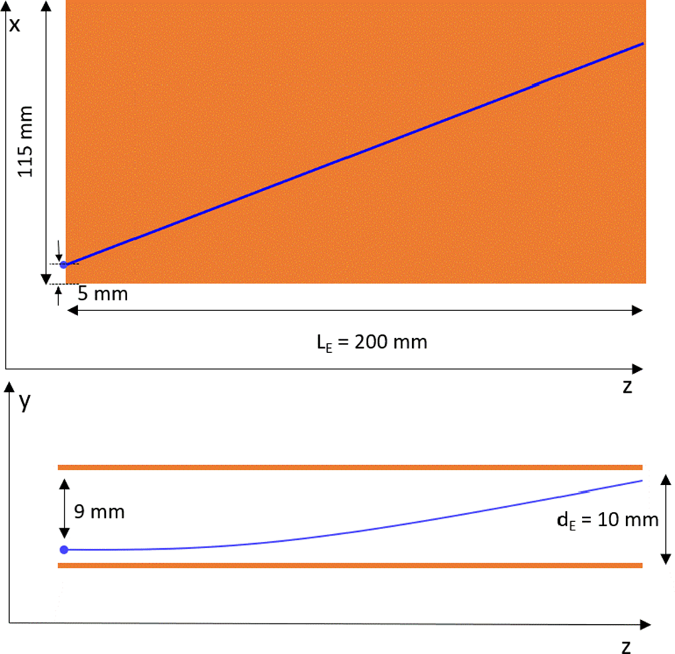
Figure 5 Dimensions of the electric field plates where the blue lines indicate the beam trajectory of 1.2 MeV protons in the capacitor.
2.1.3 Detectors and alignment laser support
The charged particles entering the spectrometer from the pinhole, are deflected by the magnetic and electric fields, cross the free-flight zone and reach the localization detector. It is expected to have different mounts according to the type of detectors used (IP, MCP, scintillator, CMOS, …). A laser diode can be temporarily fixed to the rear of the spectrometer housing, with its beam entering through a small aperture. When the laser beam is precisely aligned to traverse both the entrance and exit holes, it defines the trajectory of photons entering the spectrometer. This alignment allows the spectrometer to be accurately pointed toward the source, such as the target under investigation.
To ensure more flexibility concerning the detector part, the system has been designed such that cartridges can be inserted into the third structure. This allows for quick switching from one detector to another without having to disassemble the corresponding structure.
2.2 Simulation and analysis of the spectrometer performance
Several factors determine the TP’s energy resolution ( $\frac{\Delta E}{E}$
), including the detector’s spatial resolution, the maximum dispersion, the aperture diameter at the entrance of the TP and the divergence of the beam. The TP’s dispersion depends on the strength of the electric and magnetic fields and the charge-to-mass ratio, as well as the kinetic energy of the deflected ions. Simulations of the entire spectrometer conducted with GEANT4[
Reference Agostinelli, Allison, Amako, Apostolakis, Araujo, Arce, Asai, Axen, Banerjee, Barrand, Behner, Bellagamba, Boudreau, Broglia, Brunengo, Burkhardt, Chauvie, Chuma, Chytracek, Cooperman and Zschiesche36] allowed us to establish a dispersion relation for each charge-to-mass ratio within a specific energy range. The primary factor limiting the TP’s energy resolution is the entrance pinhole solid angle (
$\frac{\Delta E}{E}$
), including the detector’s spatial resolution, the maximum dispersion, the aperture diameter at the entrance of the TP and the divergence of the beam. The TP’s dispersion depends on the strength of the electric and magnetic fields and the charge-to-mass ratio, as well as the kinetic energy of the deflected ions. Simulations of the entire spectrometer conducted with GEANT4[
Reference Agostinelli, Allison, Amako, Apostolakis, Araujo, Arce, Asai, Axen, Banerjee, Barrand, Behner, Bellagamba, Boudreau, Broglia, Brunengo, Burkhardt, Chauvie, Chuma, Chytracek, Cooperman and Zschiesche36] allowed us to establish a dispersion relation for each charge-to-mass ratio within a specific energy range. The primary factor limiting the TP’s energy resolution is the entrance pinhole solid angle ( $<$
μsr). Thus, in all our studies, the pinhole diameter at the entrance of the TP (30 cm from the target) was set to 100 μm in the simulations. We considered in the following IP detectors with a spatial resolution of 50 μm (in the most optimistic scenario) to isolate the effects of other parameters.
$<$
μsr). Thus, in all our studies, the pinhole diameter at the entrance of the TP (30 cm from the target) was set to 100 μm in the simulations. We considered in the following IP detectors with a spatial resolution of 50 μm (in the most optimistic scenario) to isolate the effects of other parameters.
In our case, the species separation can be increased by three possible methods:
-
• increasing D ${}_{\mathrm{E}}$
;
${}_{\mathrm{E}}$
; -
• increasing the electric field strength;
-
• increasing L
${}_{\mathrm{E}}$
.


Increasing ${D}_{\mathrm{E}}$
significantly in order to improve the resolution is generally not a feasible option for several reasons. For instance, placing a spectrometer with a large
${D}_{\mathrm{E}}$
significantly in order to improve the resolution is generally not a feasible option for several reasons. For instance, placing a spectrometer with a large ${D}_{\mathrm{E}}$
inside a compact interaction chamber while maintaining a reasonable distance from the target can be challenging. Moreover, moving the detector plane much further away from the end of the electric field plates will proportionally increase the magnetic field dispersion (i.e.,
${D}_{\mathrm{E}}$
inside a compact interaction chamber while maintaining a reasonable distance from the target can be challenging. Moreover, moving the detector plane much further away from the end of the electric field plates will proportionally increase the magnetic field dispersion (i.e., ${D}_{\mathrm{B}}$
). This may be undesirable given the limited size of the detector. In addition, any modification that increases the dispersion of ion traces will reduce the surface density of the particle beam reaching the detector plane, resulting in a lower signal-to-noise ratio.
${D}_{\mathrm{B}}$
). This may be undesirable given the limited size of the detector. In addition, any modification that increases the dispersion of ion traces will reduce the surface density of the particle beam reaching the detector plane, resulting in a lower signal-to-noise ratio.
The strength of the electric field can be enhanced either by reducing the distance between the electrodes or by increasing the applied voltage. However, as seen before, the main limitation is the risk of breakdown. Based on experimental expertise, electric fields up to approximately $2\times {10}^6$
V/m can be applied in a typical experimental chamber at vacuum pressures ranging from
$2\times {10}^6$
V/m can be applied in a typical experimental chamber at vacuum pressures ranging from ${10}^{-4}$
to
${10}^{-4}$
to ${10}^{-5}$
mbar. Conversely, there are no fundamental limitations to increasing the length of the electric plates except for losing low-energy protons that can interact with plates that are too long.
${10}^{-5}$
mbar. Conversely, there are no fundamental limitations to increasing the length of the electric plates except for losing low-energy protons that can interact with plates that are too long.
The resolution power, which enables the discrimination of a p ${}^{+}$
trace from a He
${}^{+}$
trace from a He ${}^{2+}$
trace, was determined using data from GEANT4 simulations and a post-analysis performed with ROOT software[
Reference Antcheva37]. For this purpose, at each position on the magnetic deflection axis (i.e., particle energy), we checked whether an algorithm for peak detection could still distinguish between the two contributions on the electric deflection axis (Figure 6). If this condition was not met, we referred to the position on the magnetic axis to determine the maximum proton energy that could be discriminated from He
${}^{2+}$
trace, was determined using data from GEANT4 simulations and a post-analysis performed with ROOT software[
Reference Antcheva37]. For this purpose, at each position on the magnetic deflection axis (i.e., particle energy), we checked whether an algorithm for peak detection could still distinguish between the two contributions on the electric deflection axis (Figure 6). If this condition was not met, we referred to the position on the magnetic axis to determine the maximum proton energy that could be discriminated from He ${}^{2+}$
ions.
${}^{2+}$
ions.
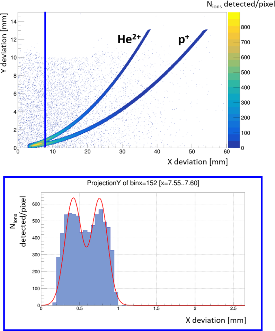
Figure 6 Top: Two-dimensional distribution of particle trajectories (X versus Y deviation in mm), showing clear separation between He ${}^{2+}$
and p
${}^{2+}$
and p ${}^{+}$
ions. The color scale indicates event density. The vertical blue line marks the last X-bin for which two distinct peaks are resolved in the Y-projection, as determined by a ROOT peak-finding algorithm. Bottom: Y-projection histogram at the selected X-bin. Two peaks correspond to He
${}^{+}$
ions. The color scale indicates event density. The vertical blue line marks the last X-bin for which two distinct peaks are resolved in the Y-projection, as determined by a ROOT peak-finding algorithm. Bottom: Y-projection histogram at the selected X-bin. Two peaks correspond to He ${}^{2+}$
and p
${}^{2+}$
and p ${}^{+}$
. The red line shows a double-Gaussian fit used for species discrimination.
${}^{+}$
. The red line shows a double-Gaussian fit used for species discrimination.
A large number of simulations were carried out to test various configurations. These simulations led us to the following optimal configuration:
-
• pinhole radius = 100 μm;
-
•
${L}_{\mathrm{B}}=40$
mm with
$B=0.76$
T; -
•
${L}_{\mathrm{E}}=200$
mm with
$E=1000$
kV/m; -
•
${D}_{\mathrm{B}}=265$
mm; -
•
${D}_{\mathrm{E}}=50$
mm; -
• total length = 300 mm.


This configuration allows us to achieve the following performances:
-
• energy resolution for p
${}^{+}$
@ 10 (100) MeV = 0.5 (1.7)
$\%$
; -
• p
${}^{+}$
/He
${}^{2+}$
discrimination possible up to 26 MeV; -
• minimum observable p
${}^{+}$
energy around 1 MeV; -
• maximum dispersion at the detector plane of 56.2 mm.


2.3 Experimental tests with IPs at the CLPU facility
Our TP was tested for TNSA shots equipped with an IP as a localization detector during a campaign on VEGA-3 at the CLPU facility [
Reference Huault, Carriere, Larreur, Nicolaï, Raffestin, Singappuli, D’Humieres, Dubresson, Batani, Cipriani, Filippi, Scisciò, Verona, Giuffrida, Kantarelou, Stancek, Boudjema, Lera, Perez-Hernández, Volpe, Frías, Bonasera, Rodrigues, Chavez, Consoli and Batani38]. The titanium-sapphire (Ti:Sa) laser VEGA-3 can deliver 30 J in a pulse duration of 30 fs at a wavelength of 800 nm. The laser spot diameter is about 11 μm full width at half maximum (FWHM) with 25 $\%$
of the energy inside the central peak. During the experiment, the pulse duration was adjusted to 200 fs, and intensity on target was
$\%$
of the energy inside the central peak. During the experiment, the pulse duration was adjusted to 200 fs, and intensity on target was $\approx$
3.5
$\approx$
3.5 $\times$
10
$\times$
10 ${}^{19}$
W/cm
${}^{19}$
W/cm ${}^2$
. A 200 μm diameter pinhole was used at the entrance of the TP, and a TR-type IP was used for the detection.
${}^2$
. A 200 μm diameter pinhole was used at the entrance of the TP, and a TR-type IP was used for the detection.
The protons and ions (C ${}^{3+}$
, C
${}^{3+}$
, C ${}^{4+}$
, O
${}^{4+}$
, O ${}^{6+}$
and C
${}^{6+}$
and C ${}^{5+}$
) were clearly detected with a minimum proton threshold energy of 0.9 MeV (see Figure 7). The ion parabolas were in agreement with predicted simulations using a map of the B-field and no significant EMP perturbations were observed. The thickness of the trace is linked to the size and conical shape of the current pinhole.
${}^{5+}$
) were clearly detected with a minimum proton threshold energy of 0.9 MeV (see Figure 7). The ion parabolas were in agreement with predicted simulations using a map of the B-field and no significant EMP perturbations were observed. The thickness of the trace is linked to the size and conical shape of the current pinhole.

Figure 7 Average over 50 shots (aluminum 8 μm targets) imaging plate scan on VEGA-3.
3 Development of an active Thomson parabola
We have explored various configurations of detection systems (part 3) based on scintillators.
The following sections present a detailed analysis of these configurations, highlighting their performance in terms of photon detection, energy resolution and practical implementation challenges. By comparing the number of photons collected and the energy resolution achieved, we aim to identify the most feasible and efficient setup for our experimental needs. In addition, we will examine in Section 3.7 the impact of different scintillator materials on detection efficiency and consider their responses to X/ $\gamma$
radiation, which is crucial for maximizing the signal-to-noise ratio and ensuring accurate ion detection.
$\gamma$
radiation, which is crucial for maximizing the signal-to-noise ratio and ensuring accurate ion detection.
This comprehensive evaluation will guide our selection of the optimal configuration for future experiments, ensuring robust and reliable performance under varying conditions.
Based on this framework, several ideas emerged to adapt our TP:
-
• use a scintillator in the detection plane with the camera in direct contact (Section 3.2);
-
• use a network of scintillating optical fibers in the detection plane to enable remote observation by the camera (Section 3.3);
-
• use a scintillator in the detection plane with remote observation through an optical fiber array (Section 3.4);
-
• use a scintillator in the detection plane with remote observation via an optical imaging system (Section 3.5).
To test and compare the performance of these different solutions, optical simulations were conducted using GEANT4, which will be briefly presented in the next section.
3.1 Optical simulation with GEANT4
When the wavelength of a photon is much greater than the atomic spacing (typically $\lambda$
= 10 nm), it can be considered as an optical photon. With GEANT4, light can be treated according to this definition (G4OpticalPhoton) independently from higher energy gamma radiation (G4Gamma). The two classes are distinct, and there are no possible transitions based on the energy of the photon. It is therefore essential to clearly define the type of photon used according to the considered energy range. Furthermore, although described in its wave aspect, the information on the phase of the photon is not managed by the simulation, making it impossible to generate potential interferences. However, such phenomena are very marginal in the case of scintillators with emission spectra spanning over several hundred nanometers.
$\lambda$
= 10 nm), it can be considered as an optical photon. With GEANT4, light can be treated according to this definition (G4OpticalPhoton) independently from higher energy gamma radiation (G4Gamma). The two classes are distinct, and there are no possible transitions based on the energy of the photon. It is therefore essential to clearly define the type of photon used according to the considered energy range. Furthermore, although described in its wave aspect, the information on the phase of the photon is not managed by the simulation, making it impossible to generate potential interferences. However, such phenomena are very marginal in the case of scintillators with emission spectra spanning over several hundred nanometers.
The different processes that can apply to optical photons are as follows:
-
• light production by scintillation (G4Scintillation) by Cherenkov emission (G4Cherenkov) or by transition radiation (G4TransitionRadiation);
-
• light attenuation during its propagation (G4Op Absorption), absorption/re-emission phenomena with wavelength shifting of photons by secondary agents (G4OpWLS);
-
• Rayleigh scattering (G4OpRayleigh);
-
• various possible interactions, such as reflection, absorption and transmission at the interfaces between two media (G4OpBoundary).
All these processes are known in their mathematical form. The optical path of light is defined by Fermat’s principle, the behavior at optical interfaces is described by Snell’s law, light attenuation in a medium is described by the Beer–Lambert law and Cherenkov radiation is also generated. These processes depend on various parameters (optical index, absorption length, reflectivity index) that each have a dependency on the wavelength of the optical photons. All of these parameters must be provided as input to the simulation. For this purpose, GEANT4 allows the creation of property tables (G4MaterialPropertiesTable) in the form of arrays of values depending on the wavelength. More details on the different properties used by this kind of simulations are given in this publication[ Reference Huber39].
In order to compare the performances of our four configurations, we simulated three different ions (p ${}^{+}$
, He
${}^{+}$
, He ${}^{1+}$
and He
${}^{1+}$
and He ${}^{2+}$
) according to a TNSA-like profile with three parameters : cutoff energy (110 MeV), temperature (E
${}^{2+}$
) according to a TNSA-like profile with three parameters : cutoff energy (110 MeV), temperature (E ${}_0$
= 30 MeV) and the different number of ions generated at a distance of 30 cm from the TP’s pinhole in a solid angle covering the latter. Figure 8 illustrates a typical example of the parabolas corresponding to these three ions when using an IP. In this configuration, we are operating under the most optimistic conditions achievable with our setup, which will serve as a reference point to assess the impact of configuration changes on the detection of these ions.
${}_0$
= 30 MeV) and the different number of ions generated at a distance of 30 cm from the TP’s pinhole in a solid angle covering the latter. Figure 8 illustrates a typical example of the parabolas corresponding to these three ions when using an IP. In this configuration, we are operating under the most optimistic conditions achievable with our setup, which will serve as a reference point to assess the impact of configuration changes on the detection of these ions.
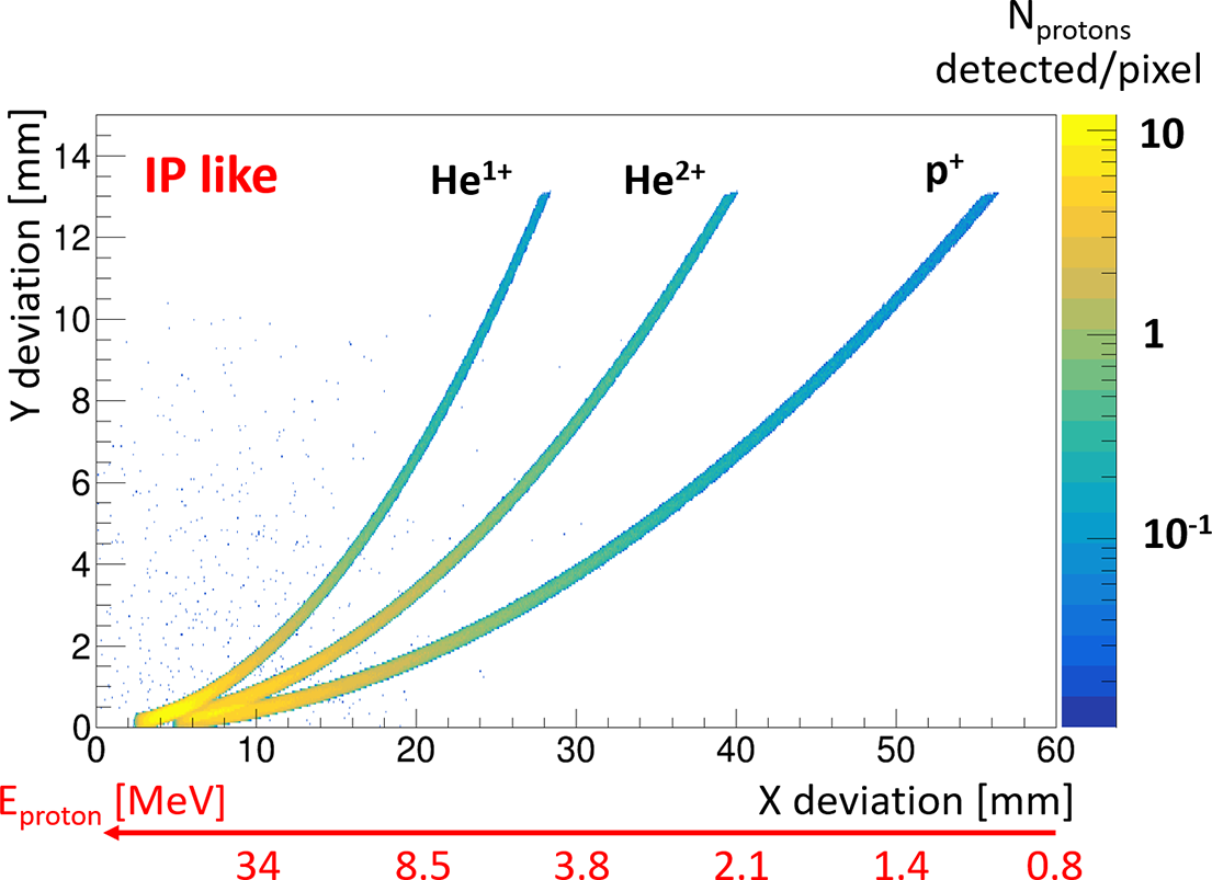
Figure 8 Simulations of p ${}^{+}$
, He
${}^{+}$
, He ${}^{1+}$
and He
${}^{1+}$
and He ${}^{2+}$
in the IP-like configuration with a pixel size of 50 μm.
${}^{2+}$
in the IP-like configuration with a pixel size of 50 μm.
Concerning the detection, we chose to work with a CMOS camera from Hamamatsu (Orca-Flash 4.0 LT Plus) with a pitch of 6.5 μm and a maximum quantum efficiency of 82 $\%$
at 560 nm. All of that will enable us to distinguish the specific effects of each parameter (configuration type, scintillator type, scintillator thickness) on the performance of the TP, such as the signal-to-noise ratio on the localization detector, the width of the traces, their possible discrimination and thus the associated energy resolution.
$\%$
at 560 nm. All of that will enable us to distinguish the specific effects of each parameter (configuration type, scintillator type, scintillator thickness) on the performance of the TP, such as the signal-to-noise ratio on the localization detector, the width of the traces, their possible discrimination and thus the associated energy resolution.
For each configuration involving a scintillator, two different thicknesses (0.1 and 1 mm) of a plastic scintillator (EJ-262) will be tested to assess the impact of this parameter on the results.
For configurations involving the fiber array, the fiber size has been set to a diameter of 200 μm, which corresponds to the minimum size of scintillating fibers sold by our supplier, Kuraray. The properties of these fibers can be found on Kuraray’s website[ 43], where the scintillator material corresponds to an EJ-212 scintillator (see Table 2 in Section 3.7). The different results presented will correspond to the round fiber multi-cladding solution. As an illustration, Figure 9 shows the simulated geometry in GEANT4 when a fiber network is used to guide the scintillator’s light to the camera.

Figure 9 Trajectory of a 2 MeV proton through the TP in GEANT4 in the case where a scintillator is in the detection with a remote observation via an optical fiber array.
For clarity purposes, we will first present the results specific to each configuration for a given scintillator (EJ-262) and the two tested thicknesses in order to better identify the sensitivity of the TP with these parameters (Sections 3.2, 3.3, 3.4 and 3.5). Following these sections, we will attempt to compare and summarize what these simulations can teach us (Section 3.6), before concluding with the impact on the results when changing the type of scintillator (Section 3.7).
3.2 Scintillator with camera in contact
This configuration, the simplest to set up, allows for optimal optical performance while minimizing space requirements. The simulation results are shown in Figures 10 and 11, which correspond to scintillators of 0.1 and 1 mm, respectively.

Figure 10 Optical simulations of p ${}^{+}$
, He
${}^{+}$
, He ${}^{1+}$
and He
${}^{1+}$
and He ${}^{2+}$
in the configuration with the camera in direct contact with a 0.1 mm EJ-262 scintillator. The binning corresponds to the pitch of our camera (6.5 μm).
${}^{2+}$
in the configuration with the camera in direct contact with a 0.1 mm EJ-262 scintillator. The binning corresponds to the pitch of our camera (6.5 μm).

Figure 11 Optical simulation of p ${}^{+}$
, He
${}^{+}$
, He ${}^{1+}$
and He
${}^{1+}$
and He ${}^{2+}$
in the configuration with the camera in direct contact with a 1 mm EJ-262 scintillator. The binning corresponds to the pitch of our camera (6.5 μm).
${}^{2+}$
in the configuration with the camera in direct contact with a 1 mm EJ-262 scintillator. The binning corresponds to the pitch of our camera (6.5 μm).
The most striking observation is the significant increase in background noise across the entire camera compared to detection via IP. This is not surprising, however, given that scintillation is emitted within a 4 $\pi$
solid angle, and the proximity of the camera to the scintillator results in the near-total detection of all produced photons from the scintillator, making the trace broader. This effect becomes even more pronounced when the scintillator is thicker, as the photons have more space to propagate, thereby increasing the dispersion of their detection points relative to their emission points. Indeed, without an optical system, the detection plane on the camera will correspond to the exit plane of the scintillator. As a result of this effect, we can see a loss of information about the high-energy ions when the scintillator thickness is 1 mm. In addition, the traces tend to thicken for the lowest energies, as the ions are stopped in the first layers of the scintillator, which subsequently increases the dispersion of photons reaching the camera. When this phenomenon is minimized by reducing the thickness of the scintillator, we observe in Figure 10 that access to different information remains possible, despite a slight increase in the trace width.
$\pi$
solid angle, and the proximity of the camera to the scintillator results in the near-total detection of all produced photons from the scintillator, making the trace broader. This effect becomes even more pronounced when the scintillator is thicker, as the photons have more space to propagate, thereby increasing the dispersion of their detection points relative to their emission points. Indeed, without an optical system, the detection plane on the camera will correspond to the exit plane of the scintillator. As a result of this effect, we can see a loss of information about the high-energy ions when the scintillator thickness is 1 mm. In addition, the traces tend to thicken for the lowest energies, as the ions are stopped in the first layers of the scintillator, which subsequently increases the dispersion of photons reaching the camera. When this phenomenon is minimized by reducing the thickness of the scintillator, we observe in Figure 10 that access to different information remains possible, despite a slight increase in the trace width.
Firstly, there is the need to use thin scintillators to avoid degrading the energy resolution (discussion in Section 3.6). Secondly, if the scintillator is thin, energetic ions could pass through the scintillator and interact with the camera. Beyond the difficulty of evaluating the impact of ions on the camera compared to the detected photon signal, this could primarily result in potential damage to the detector according to the laser power configuration. Fuchs et al. [ Reference Burdonov, Lelievre, Forestier-Colleoni, Ceccotti, Cuciuc, Lancia, Yao and Fuchs44] reported the absolute calibration of a CMOS detector with particles created by a 8.1 J per pulse laser. The use of CMOS detectors at higher laser energies such as the ones expected at the APOLLON facility is still to be demonstrated. Thirdly, a compact solution such as this can also raise issues of EMP management.
3.3 Scintillating fibers imaged by a camera
At first glance, this configuration seemed to be the most promising of all. Indeed, this configuration allows for the optimal transfer of light while enabling the measurement to be moved outside the experimental chamber to avoid issues related to residual gas analysis (RGA) and EMPs.
However, the simulations of the TP with all the fibers considered (with a 1 m length) quickly revealed a major problem, shown in Figure 12. Beyond a certain energy (30 MeV in our example, which corresponds to a deviation of $\sim$
10 mm along the x-axis), protons are energetic enough to deposit energy in one fiber, pass through it, and then deposit the rest of their energy in one or more other fibers. This results in significant smearing in a region where energy resolution is crucial. Therefore, it could be difficult to use this type of configuration for experiments aiming to measure protons with energies above 30 MeV. However, it is worth noting that this phenomenon occurs within an energy range where discrimination is no longer achievable with IPs, which could ultimately limit the impact of this phenomenon on the obtained results.
$\sim$
10 mm along the x-axis), protons are energetic enough to deposit energy in one fiber, pass through it, and then deposit the rest of their energy in one or more other fibers. This results in significant smearing in a region where energy resolution is crucial. Therefore, it could be difficult to use this type of configuration for experiments aiming to measure protons with energies above 30 MeV. However, it is worth noting that this phenomenon occurs within an energy range where discrimination is no longer achievable with IPs, which could ultimately limit the impact of this phenomenon on the obtained results.
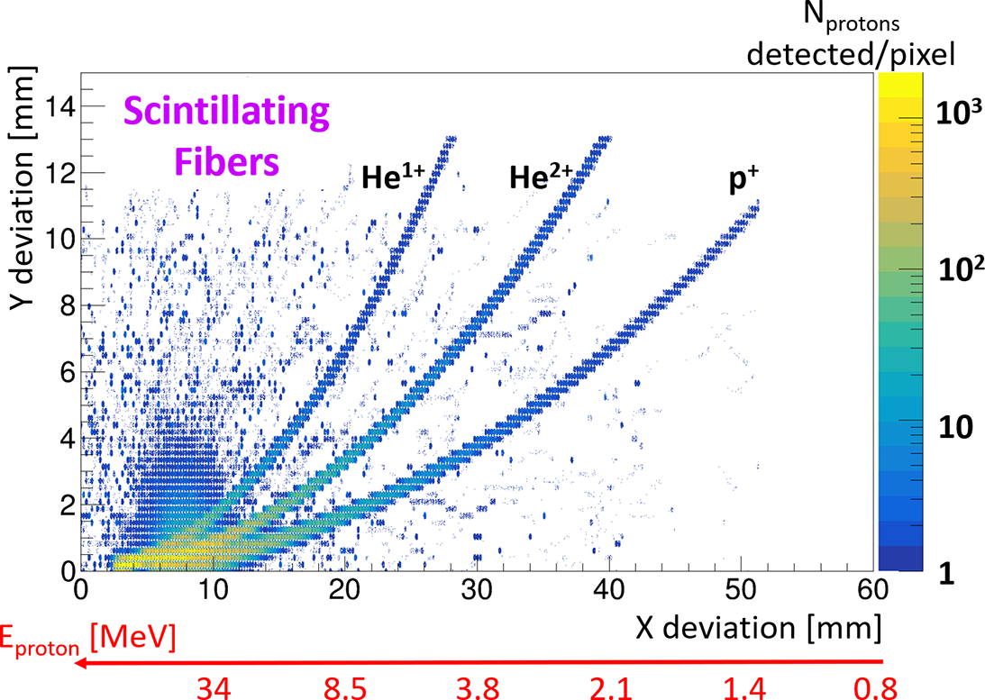
Figure 12 Optical simulations of p ${}^{+}$
, He
${}^{+}$
, He ${}^{1+}$
and He
${}^{1+}$
and He ${}^{2+}$
in the configuration where scintillating fibers (pitch of 200 μm) are imaged by a camera. The binning corresponds to the pitch of our camera (6.5 μm).
${}^{2+}$
in the configuration where scintillating fibers (pitch of 200 μm) are imaged by a camera. The binning corresponds to the pitch of our camera (6.5 μm).
In any case, for experiments not targeting these energy ranges, the energy resolution will not only depend on the camera’s pitch but also on the pitch of the fibers, which currently cannot go below 200 μm due to its design with the scintillating material as the core within the fiber.
3.4 Light from scintillator collected by a fiber network and imaged by a camera
This configuration is similar to the previous one, except that an array of fibers with a 200 μm pitch is installed to create the connection between the scintillator and the camera (see Figure 9). The simulation results are shown in Figures 13 and 14, which correspond to scintillators of 0.1 and 1 mm, respectively.

Figure 13 Optical simulations of p ${}^{+}$
, He
${}^{+}$
, He ${}^{1+}$
and He
${}^{1+}$
and He ${}^{2+}$
in the configuration where the photons emitted by a scintillator of 0.1 mm are collected with a bunch of fibers with a pitch of 200 μm. The binning corresponds to the pitch of our camera (6.5 μm).
${}^{2+}$
in the configuration where the photons emitted by a scintillator of 0.1 mm are collected with a bunch of fibers with a pitch of 200 μm. The binning corresponds to the pitch of our camera (6.5 μm).

Figure 14 Optical simulations of p ${}^{+}$
, He
${}^{+}$
, He ${}^{1+}$
and He
${}^{1+}$
and He ${}^{2+}$
in the configuration where the photons emitted by a scintillator of 1 mm are collected with a bunch of fibers with a pitch of 200 μm. The binning corresponds to the pitch of our camera (6.5 μm).
${}^{2+}$
in the configuration where the photons emitted by a scintillator of 1 mm are collected with a bunch of fibers with a pitch of 200 μm. The binning corresponds to the pitch of our camera (6.5 μm).
Overall, the same effects as in the first configuration (scintillator and camera in contact) can be observed, which is not surprising given the geometric similarity between the two configurations. However, using the fiber array will necessarily result in fewer photons being detected by the camera compared to the direct contact configuration (factor of 10–100) due to the influence of the numerical aperture (NA) of the fibers and the loss of some photons during their propagation within the fibers (detailed below in Figure 18). Nevertheless, the NA of the fibers also helps filter out certain unwanted photons, thereby slightly reducing the background noise on our camera. This makes it possible to increase the thickness of the scintillator to improve sensitivity (unlike the first configuration), although some broadening of the tracks at the detector is still observed. We will discuss this in more detail in Section 3.6.
This configuration appears to be quite promising as it allows for the maximization of light transfer from the scintillator to the camera while also enabling the camera to be installed outside the experimental chamber, thereby resolving potential issues related to RGA and EMPs. Regarding light disturbances from the environment, light tightness can be achieved with this type of structure. However, it is essential to use thin scintillators to avoid deteriorating energy resolution, especially since it will already be degraded due to the use of fiber for which the pitch is larger than those of the camera. If this solution is used, it will be necessary to consider this effect in combination with the significant increase in the number of fibers to transport if one aims to approach the camera’s pitch. For example, the simulation shown in Figures 13 and 14 with a 200 μm pitch corresponds to a total of 6250 fibers. Reducing the pitch to 50 μm (the parameter used in IP analysis), for example, would increase this total to 100,000 fibers.
3.5 Scintillator imaged by an optical system on camera
This last configuration relies on an optical lens-based system to collect photons emitted from the scintillator and image them on the camera plane (Figure 15) with a given detection solid angle according to the localization of energy deposition[ Reference Seemann, Wan, Tata, Kroupp and Malka33]. The distance between the emission point and the TP’s pinhole is still the same (30 cm) and we will incorporate a virtual biconvex lens (f = 300 mm, NA = 0.13) at a distance of 30 cm from the scintillator’s exit plane. Thus, detecting the photons on the lens while recording information about their momentum will allow us to reconstruct, similar to the optical function of the lens, the point at which the photons exit the scintillator. The diameter and distance concerning the lens are arbitrary but correspond to use cases that could be implemented with common lenses and objectives.

Figure 15 Schematic view of an experiment presenting the various dimensions of interest.
The simulation results are shown in Figures 16 and 17, which correspond to scintillators of 0.1 and 1 mm, respectively.
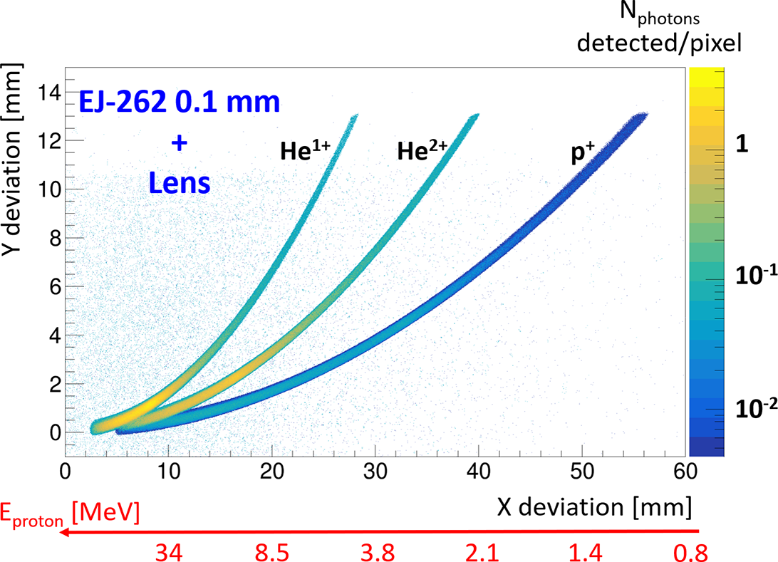
Figure 16 Optical simulations of p ${}^{+}$
, He
${}^{+}$
, He ${}^{1+}$
and He
${}^{1+}$
and He ${}^{2+}$
in the configuration where the photons emitted by a scintillator of 0.1 mm are collected with an optical system. The binning corresponds to the pitch of the camera (6.5 μm).
${}^{2+}$
in the configuration where the photons emitted by a scintillator of 0.1 mm are collected with an optical system. The binning corresponds to the pitch of the camera (6.5 μm).
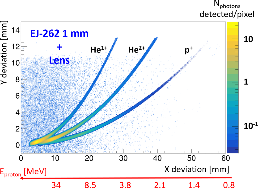
Figure 17 Optical simulations of p ${}^{+}$
, He
${}^{+}$
, He ${}^{1+}$
and He
${}^{1+}$
and He ${}^{2+}$
in the configuration where the photons emitted by a scintillator of 1 mm are collected with an optical system. The binning corresponds to the pitch of the camera (6.5 μm).
${}^{2+}$
in the configuration where the photons emitted by a scintillator of 1 mm are collected with an optical system. The binning corresponds to the pitch of the camera (6.5 μm).

Figure 18 Number of photons collected per pixel and per detected proton as a function of incident proton energy for different thicknesses of EJ-262 scintillators. The width of the curves corresponds to an uncertainty of 10 $\%$
.
$\%$
.
Unlike the previous configuration, it can be observed that, this time, increasing the thickness of the scintillator does not cause any great impact concerning the noise or the broadening of the trace. This can be explained by a simple geometric description of the phenomenon. Indeed, even though photon scattering is more significant for a thicker scintillator, the solid angle of collection of the lens remains the same, which only impacts the number of photons collected by the lens. However, the decrease in the number of photons collected for a thicker scintillator can be compensated for certain energies by the fact that more photons will be produced when ions interact with the scintillator if they do not pass through it completely. We will discuss this in the next section.
In conclusion, this configuration is very interesting because it allows the thickness of the scintillator to be adapted based on the experiment and the expected energy ranges without degrading the energy resolution. However, it is important to keep in mind the loss of light caused at low energies when increasing the thickness of the scintillator. The use of an optical system to displace the light collection is also advantageous in addressing the RGA and EMP issues mentioned in the previous section. In addition, the displacement would allow the use of filters to eliminate potential light noises by applying spectral filters that transmit light from the scintillator but strongly attenuate other wavelengths. Of course, this kind of filter was not used in our simulations. Nevertheless, it is also important to keep in mind that the image obtained on the camera could correspond to a given plane of the scintillator depending on the focal depth of the imaging system. In addition, one must consider the potential significant loss of photons depending on the solid angle of the optical system’s collection, which could be crucial in certain cases. We will return to this point during the tests conducted for the characterization of scintillators in Appendix A.
3.6 Configurations summary
Now that we have characterized the response of each of our configurations, we will attempt to compare them. To do this, let us begin by comparing the number of photons collected in these different simulations. We obtain Figure 18, which shows the evolution of the number of photons detected per pixel and per detected proton as a function of the proton energy for our different simulation configurations. We observe, firstly, that the amplitude of the range is very large (five orders of magnitude) between the two extreme configurations, namely the 1 mm scintillator in direct contact with the camera and the light collection from the scintillator via an optical device placed 30 cm away. We also note that, as expected, the configurations with fibers fall within intermediate ranges. It is also worth mentioning the shift in the Bragg peak (around 15 MeV) when the scintillator thickness changes, observed for the two different thickness configurations tested.
However, we observed that the number of collected photons is not a sufficient variable to determine the feasibility of a configuration. Indeed, we noted, particularly for configurations with a large number of detected photons in Figure 18, that this was accompanied by a possible degradation of our tracks, and therefore a potential degradation in energy resolution as well as a possible loss of information regarding ion discrimination.
Thus, Figure 19 shows the evolution of the relative energy resolution as a function of the energy of a proton for our different tested configurations. These results are also compared to the most optimistic case achievable with our setup, which corresponds to the configuration with the IPs.

Figure 19 Energy resolution $\frac{\Delta E}{E}$
expected as a function of incident proton energy for different thicknesses of EJ-262 scintillators and comparison with the IP configuration.
$\frac{\Delta E}{E}$
expected as a function of incident proton energy for different thicknesses of EJ-262 scintillators and comparison with the IP configuration.
To synthesize the findings from all tested detection configurations, Table 1 summarizes their main characteristics, including signal level, resolution, practical feasibility and robustness under experimental conditions. This overview facilitates the comparison and highlights trade-offs relevant for experimental design.
Table 1 Summary of performance for the tested detection configurations.

Table 2 Scintillation properties of three different scintillators (organic, phosphorous and inorganic). For EJ-444, values in parentheses correspond to the organic part (EJ-212).

Based on this table, we can affirm that using a scintillator in direct contact with a camera is hardly feasible (optimistic case without considering proton interactions in the camera, potential damage and significant background noise).
We can also observe that it remains preferable, in order to avoid affecting the energy resolution, to use scintillators with thicknesses of the order of 100 μm. The gain in detected photon sensitivity is not substantial and could potentially lead to a higher degradation in the scintillator bulk due to the Bragg peak. Favoring thinner scintillators allows us to minimize this effect while maximizing the number of ions passing through.
There are then three configurations, each with its advantages and drawbacks depending on what we aim to measure. Indeed, aside from potential effects at very high energies, fiber scintillators remain an interesting configuration due to their high sensitivity without degrading the energy resolution within the considered range. However, the implementation of such a detection system remains the greatest challenge of this configuration due to the management of a large number of fibers. This also applies to the configuration with non-scintillating fibers combined with a scintillator, where the results still fall within the intermediate range.
The final configuration with an optical lens-based system, despite suffering from potential sensitivity issues, remains the most attractive solution overall, given its ease of implementation and excellent results regarding track quality. This is why, in the section concerning our experimental tests (Appendix A), we chose to use this configuration.
3.7 Comparative study of scintillator materials
Now that we have seen the impact of different configurations on scintillation light detection by our system, we will examine, in the context of the configuration with the optical system, the differences observed for the various scintillators mentioned in Table 2 (organic, phosphor and inorganic). It is important to notice that EJ-444 consists of a thin piece of EJ-212 plastic scintillator (0.1 or 1 mm in our case) with a layer ( $\approx$
40 μm) of silver-activated zinc sulfide phosphor (ZnS:Ag) applied to one side. Since we have already characterized the impact of thicknesses for each configuration, we will focus this time on the situation where the scintillator has a thickness of 0.1 mm.
$\approx$
40 μm) of silver-activated zinc sulfide phosphor (ZnS:Ag) applied to one side. Since we have already characterized the impact of thicknesses for each configuration, we will focus this time on the situation where the scintillator has a thickness of 0.1 mm.
Logically, it is essential to account for the quenching effect of the luminescent sites within a scintillator in order to quantitatively describe the light yield. This phenomenon can be modeled in GEANT4 simulations by incorporating a Birks’ constant. The impact of this effect becomes even more significant for heavier particles, as they deposit more energy per unit volume. However, defining an appropriate Birks’ constant in GEANT4 is highly dependent on specific simulation parameters and typically requires calibration with experimental data[ Reference Huber39]. For this reason, in the context of this qualitative study, we adopted an ultra-optimistic scenario in which scintillation quenching is neglected.
Thus, we obtain Figure 20, which shows the number of photons detected per pixel and per particle that has deposited energy in the scintillator, as a function of the incident energy of the protons for three scintillators (EJ-262, EJ-444 and YAG). It can be easily seen that the maximum energy deposited in the scintillator (which corresponds to the limit case of the proton passing through) is around 4–5 MeV for protons when the scintillator has a thickness of 0.1 mm. As expected, given the light yields of these scintillators, the higher the light yield, the greater the number of photons detected, which favors YAG.
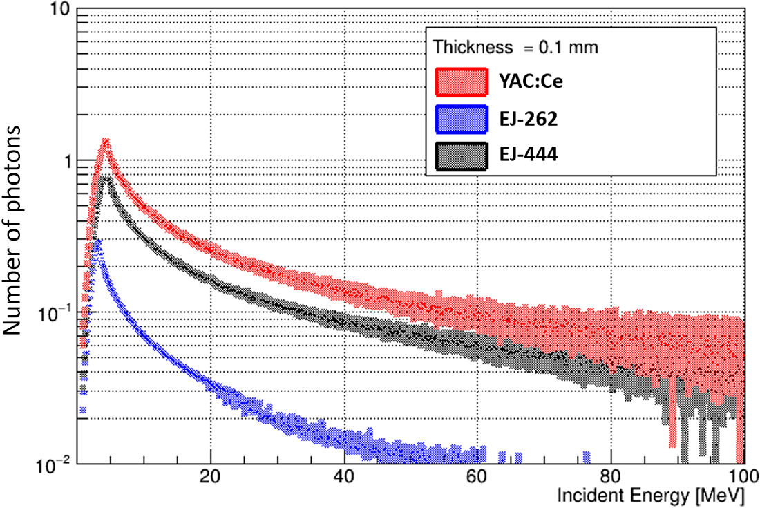
Figure 20 Number of photons collected per pixel and per detected proton as a function of incident proton energy for different scintillators (EJ-262, EJ-444 and YAG:Ce) for a thickness of 0.1 mm in the lens configuration.
Regarding energy resolution, the simulation does not show significant variations depending on the choice of scintillator. Thus, the energy resolution will mainly be impacted by the configuration and/or the thickness of the scintillator rather than by the type of scintillator used (Figure 19).
Another point to consider is the response of these scintillators to X/ $\gamma$
radiation emitted during the laser shot. Indeed, if these radiations are detected in too large a number, they may increase background noise on the camera, making ion detection more difficult. To provide an answer to this question, we simulated an X/
$\gamma$
radiation emitted during the laser shot. Indeed, if these radiations are detected in too large a number, they may increase background noise on the camera, making ion detection more difficult. To provide an answer to this question, we simulated an X/ $\gamma$
flash at 30 cm from the detector system following a Boltzmann distribution with a temperature E
$\gamma$
flash at 30 cm from the detector system following a Boltzmann distribution with a temperature E ${}_0$
= 805 keV[
Reference Norreys, Santala, Clark, Zepf, Watts, Beg, Krushelnick, Tatarakis, Dangor, Fang, Graham, McCanny, Singhal, Ledingham, Creswell, Sanderson, Magill, Machacek, Wark, Allott, Kennedy and Neely45]. Table 3 presents the detection efficiencies obtained for our three scintillators. Naturally, the higher the density and atomic number (Z) of the material, the greater the probability that X/
${}_0$
= 805 keV[
Reference Norreys, Santala, Clark, Zepf, Watts, Beg, Krushelnick, Tatarakis, Dangor, Fang, Graham, McCanny, Singhal, Ledingham, Creswell, Sanderson, Magill, Machacek, Wark, Allott, Kennedy and Neely45]. Table 3 presents the detection efficiencies obtained for our three scintillators. Naturally, the higher the density and atomic number (Z) of the material, the greater the probability that X/ $\gamma$
radiation will interact with the scintillator. This explains why the organic scintillator, made of hydrogen and carbon with a density close to 1, is the most transparent to this radiation, which could prove crucial in certain experiments, despite having a lower yield than cerium-doped yttrium aluminum garnet (YAG:Ce).
$\gamma$
radiation will interact with the scintillator. This explains why the organic scintillator, made of hydrogen and carbon with a density close to 1, is the most transparent to this radiation, which could prove crucial in certain experiments, despite having a lower yield than cerium-doped yttrium aluminum garnet (YAG:Ce).
Table 3 Estimation of the X/ $\gamma$
radiation detection probability for three different scintillators (EJ-262, EJ-444 and YAG:Ce). The X/
$\gamma$
radiation detection probability for three different scintillators (EJ-262, EJ-444 and YAG:Ce). The X/ $\gamma$
distribution simulated corresponds to a Boltzmann distribution with E
$\gamma$
distribution simulated corresponds to a Boltzmann distribution with E ${}_0$
= 805 keV.
${}_0$
= 805 keV.

Given this point, one may wonder whether it will always be possible, during data analysis, to determine the zero-deflection point using the interaction of X/ $\gamma$
rays generated during the laser shot for a plastic scintillator. Simulations indicate that there is a factor of 10 million between the energy deposited by a traversing proton (without applying quenching) and that deposited by an X/
$\gamma$
rays generated during the laser shot for a plastic scintillator. Simulations indicate that there is a factor of 10 million between the energy deposited by a traversing proton (without applying quenching) and that deposited by an X/ $\gamma$
beam following the Boltzmann distribution described earlier. If we are able to detect of the order of 10–100 protons per detection zone, this implies that a minimum gamma flux of 10
$\gamma$
beam following the Boltzmann distribution described earlier. If we are able to detect of the order of 10–100 protons per detection zone, this implies that a minimum gamma flux of 10 ${}^9$
photons on the scintillator would be required to produce a visible image on the detector. However, if such a signal were not observable, the modularity of our TP, combined with the laser alignment system, would still allow us to constrain the origin point. Indeed, the ability to switch detectors without altering the rest of the TP makes it possible to perform a prior calibration using an IP of identical dimensions to locate and define the zero-deflection point.
${}^9$
photons on the scintillator would be required to produce a visible image on the detector. However, if such a signal were not observable, the modularity of our TP, combined with the laser alignment system, would still allow us to constrain the origin point. Indeed, the ability to switch detectors without altering the rest of the TP makes it possible to perform a prior calibration using an IP of identical dimensions to locate and define the zero-deflection point.
In addition, we have already mentioned several times the need to pass the RGA tests required to access certain facilities. These tests are due to be conducted soon to determine whether or not these scintillators can be introduced into a vacuum chamber according to the criteria of these facilities even if we already know that it is possible with a YAG:Ce scintillator[ Reference Burdonov, Fazzini, Lelasseux, Albrecht, Antici, Ayoul, Beluze, Cavanna, Ceccotti, Chabanis, Chaleil, Chen, Chen, Consoli, Cuciuc, Davoine, Delaneau, D’humières, Dubois, Evrard, Filippov, Freneaux, Forestier-Colleoni, Gremillet, Horny, Lancia, Lecherbourg, Lebas, Leblanc, Ma, Martin, Negoita, Paillard, Papadopoulos, Perez, Pikuz, Qi, Quéré, Ranc, Söderström, Scisciò, Sun, Vallières, Wang, Yao, Mathieu, Audebert and Fuchs18].
Another important parameter is the cost of these scintillators. While the prices of ELJEN scintillators (EJ-262 and EJ-444) are in the region of several hundred euros depending on size and thickness, the price of a YAG scintillator of the same dimensions is multiplied by a factor of 8–10, which is significant, especially as we currently lack information on the durability of these scintillators when exposed to high-repetition-rate particle fluxes (other than electrons) in laser–plasma experiments. Appendix A will attempt to address this question through tests conducted on the AIFIRA platform of LP2IB to characterize these three scintillators.
4 Conclusion
In this work, we described the design of a modulable and active TP where all the components have been discussed in detail. The design of the spectrometer is conceived in such a way that the TP elements can be easily adapted to different experimental conditions that may be encountered. In addition, this TP is also built for an easy and quick mounting and includes a built-in alignment device for faster setup and reliable operation in the experiments.
Moreover, through optical simulations conducted using GEANT4, we tested various configurations of ‘active’ detection, and these results allowed us to determine that certain solutions were not feasible. This was particularly true for direct scintillation detection with a contact detector or the use of a bundle of scintillating fibers.
However, it remains necessary to test our TP in its active mode under real conditions while continuing to develop optical simulations. This will ensure the most comprehensive monitoring of scintillation and guarantee both qualitative and quantitative measurements.
Appendix A Scintillator characterization on the AIFIRA platform
A.1 Experimental setup
AIFIRA[
Reference Barberet, Jouve and Sorieul46] (Applications Interdisciplinaires des Faisceaux d’Ions en Région Aquitaine) is a compact ion beam facility equipped with a single-stage electrostatic accelerator that delivers beams of light ions (protons, deuterons and helium) in the MeV energy region. Commissioned in 2006, the accelerator (3.5 MV SingletronTM from HVEE, the Netherlands) provides beams with high brightness (20 A m ${}^{-2}$
rad
${}^{-2}$
rad ${}^{-2}$
eV
${}^{-2}$
eV ${}^{-1}$
) and excellent energy stability (
${}^{-1}$
) and excellent energy stability ( $\Delta E/E={10}^{-5}$
) across five beamlines dedicated to specific applications.
$\Delta E/E={10}^{-5}$
) across five beamlines dedicated to specific applications.
For our tests, we utilized the microbeam line at AIFIRA. This line features a two-stage magnetic quadrupole quintuplet focusing system, and the analysis chamber is equipped with surface-barrier detectors for conducting RBS (Rutherford backscattering spectroscopy) and NRA (nuclear reaction analysis) experiments, as well as on-axis scanning transmission ion microscopy (STIM) for thin targets. The samples are mounted on an XYZ motorized stage with micrometer positioning accuracy. A set of microscope objectives paired with video cameras allows for in situ visualization of the sample at various magnifications. The microbeam can achieve a spot diameter of 1 μm in high-current mode (several hundred pA) and 0.3 μm in low-current mode (a few thousand counts per second). A custom-made electrostatic system is employed to raster scan the beam spot across the sample surface for imaging purposes.
For our study, we selected a proton energy of 2.5 MeV to maximize the energy deposition in our 0.1 mm plastic scintillators[ 47]. The beam size was 1 μm in diameter, and we used fluxes ranging from 0.3 to 5 pA. The integration time of the Hamamatsu camera (Orca-Flash 4.0 LT Plus) was also adjusted (from 3.5 ms to 10 s) to vary the number of integrated protons. Five scintillators were tested:
-
• EJ-262: 0.1 and 1 mm;
-
• EJ-444: 0.1 and 1 mm (approximately 50 μm ZnS + 0.1/1 mm EJ-212);
-
• YAG:Ce: 0.1 mm.
The images were recorded in .tiff format and then converted to .csv format (in gray value (Gv)) for analysis using the ROOT software (Figure 21).

Figure 21 Example of results obtained with (a) the adjustment of the distribution obtained following the irradiation of a scintillator and (b) the details of the adjustment and the different components when projected onto the x-axis at the maximum level signal.
A background noise measurement was taken at the beginning of each day to subtract the camera noise from our raw (RAW) data. This allows us to obtain the signal associated solely with scintillation (TRUE). The resulting distribution is then fitted with a double Gaussian in two dimensions, as shown in Figure 21(a). Figure 21(b), which represents the pixel projection along the x-axis of the two-dimensional (2D) distribution at the point where the signal is maximum, allows us to observe the different contributions mentioned (RAW signal in black, TRUE signal in cyan, double-Gaussian fit in red, Gaussian fit corresponding to the signal in green and Gaussian fit of the noise caused by light scattering in the scintillator in gray). The fitting enables us to estimate the number of integrated Gvs recorded by the camera that correspond to our signal. We will discuss the various observed results in the following section.
A.2 Results
A.2.1 Measurement behavior for large numbers of protons detected
We previously mentioned the need to perform a 2D double-Gaussian fit to account for the ‘noise’ caused by photon scattering within the scintillator. Figure 22, which corresponds to higher proton fluxes, will help us visualize this phenomenon by comparing it with Figure 21(b). Indeed, in the first figure, the maximum number of integrated Gvs is around 12,000, compared to 200 in the first example. This means that a much larger number of photons were detected in response to a higher number of protons integrated over the acquisition period. The double-Gaussian fit is still well-executed and is even indispensable in this specific case. Since a significantly higher number of photons were produced, more and more detected photons correspond to those that could have scattered within the scintillator, resulting in increased noise caused by these photons, as seen in the gray contribution.

Figure 22 Effects on signal width distribution when a large number of protons are detected.
A.2.2 Scintillation degradation
We also took advantage of the proton beam to characterize the degradation of scintillation when the scintillator is exposed to a continuous proton flux of 2.5 MeV at a flux of 380 fA ( $\approx$
2.4
$\times$
10
$\approx$
2.4
$\times$
10 ${}^6$
p
${}^6$
p ${}^{+}$
/s). A long-duration acquisition of 400 s was carried out with the Hamamatsu camera. Regular analysis at fixed intervals of the obtained image enabled us to reconstruct the evolution of the number of integrated Gvs as a function of incident protons on the scintillator. The loss of light due to the degradation of the scintillator will correspond to a lower number of protons detected than we expect, as shown in Figure 23. For our conditions, the degradation begins to appear around 10
${}^{+}$
/s). A long-duration acquisition of 400 s was carried out with the Hamamatsu camera. Regular analysis at fixed intervals of the obtained image enabled us to reconstruct the evolution of the number of integrated Gvs as a function of incident protons on the scintillator. The loss of light due to the degradation of the scintillator will correspond to a lower number of protons detected than we expect, as shown in Figure 23. For our conditions, the degradation begins to appear around 10 ${}^6$
integrated protons with a 1 mm beam diameter, which is far beyond what the scintillator should be confronted with under experimental conditions. The same overall effect was observed with EJ-444, and it will be necessary in a future campaign to also perform this measurement with YAG:Ce.
${}^6$
integrated protons with a 1 mm beam diameter, which is far beyond what the scintillator should be confronted with under experimental conditions. The same overall effect was observed with EJ-444, and it will be necessary in a future campaign to also perform this measurement with YAG:Ce.
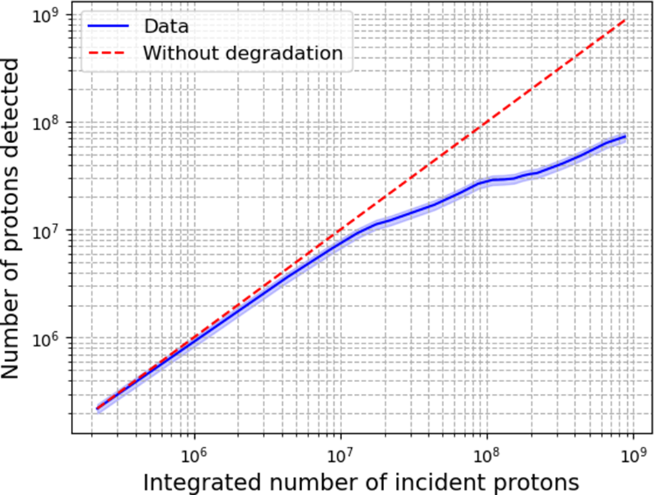
Figure 23 Evolution of the number of protons detected according to the integrated number of incident protons (at a flux of 380 fA), which characterize the degradation of scintillator EJ-262 under proton irradiation on a 1 μm diameter spot.
When performing a test with a flux 1000 times higher on EJ-262, we even observed permanent degradation of the scintillator with a darkened area in the center of the window. It seems that the scintillator was significantly damaged, particularly due to the high concentration of energy deposition in one spot induced by the Bragg peak. Several explanations for this phenomenon are possible, such as a reduction in optical transmission (due to effects on the plastic based material) and/or a decrease in emission due to the degradation of the scintillating component[ Reference Green, Scott, Neely and Parker48]. The data from this paper are in agreement with what we observed with our EJ-262 scintillator.
These findings highlight an important factor when using this type of system in experiments that may be subjected to high particle fluxes, especially for ions. Indeed, as seen in Figure 23, it is essential and mandatory to regularly calibrate the detector’s energy response to correctly estimate the number of incident particles.
A.2.3 Light response calibration
To eliminate undesirable effects related to variations in scintillation, each measurement was conducted with a brief exposure of around 30 s for the scintillator to limit the strong variations at the beginning of irradiation.
The measurements for our five scintillators are shown in Figure 24, which represents the number of integrated Gvs as a function of the number of protons emitted per unit area and within a solid angle corresponding to that between the scintillator and the lens that collects the light and transmits to the camera. In our case, the number of protons is determined from the flux, the emission area is based on the beam size (1 mm diameter) and the solid angle of detection was approximately 1.88 sr (microscope objective LUCPLFLN 20x used).

Figure 24 Evolution of the integrated gray value detected according to the proton flux for our five scintillators tested. Limits corresponding to a decision threshold with an $\alpha$
value of 10
$\alpha$
value of 10 $\%$
are also displayed.
$\%$
are also displayed.
The first observation is that all the scintillators’ responses are indeed linear. The second observation, as mentioned earlier (see Figure 20), clearly shows that YAG is the most efficient scintillator, followed by ZnS (EJ-444) and finally EJ-262. As expected, if the thickness of the scintillator increases, this results in a decrease in the number of detected photons in our specific case where the proton is supposed to deposit all its energy within the first 100 μm.
Furthermore, we estimated, based on the dimensions of the spots observed for each scintillator, an upper limit on the number of integrated Gvs required to reject the hypothesis that we are only measuring background noise with a confidence level of 90 $\%$
[
Reference Weise, Hübel, Rose, Schläger, Schrammel, Täschner and Michel49]. These limits correspond to the horizontal dashed lines, which then enable us to estimate the minimum flux required to observe a signal when integrating the entire image.
$\%$
[
Reference Weise, Hübel, Rose, Schläger, Schrammel, Täschner and Michel49]. These limits correspond to the horizontal dashed lines, which then enable us to estimate the minimum flux required to observe a signal when integrating the entire image.
Acknowledgements
This study has received financial support from the French State in the framework of the Investments for the Future programme IdEx université de Bordeaux/GPR LIGHT.
This project has received funding from the European Union’s Horizon 2020 Research and Innovation Programme under grant agreement no. 871124 Laserlab-Europe.
The AIFIRA facility is financially supported by the CNRS, the university of Bordeaux and the Région Nouvelle Aquitaine. We thank the technical staff members of the AIFIRA facility, P. Alfaurt and S. Sorieul.

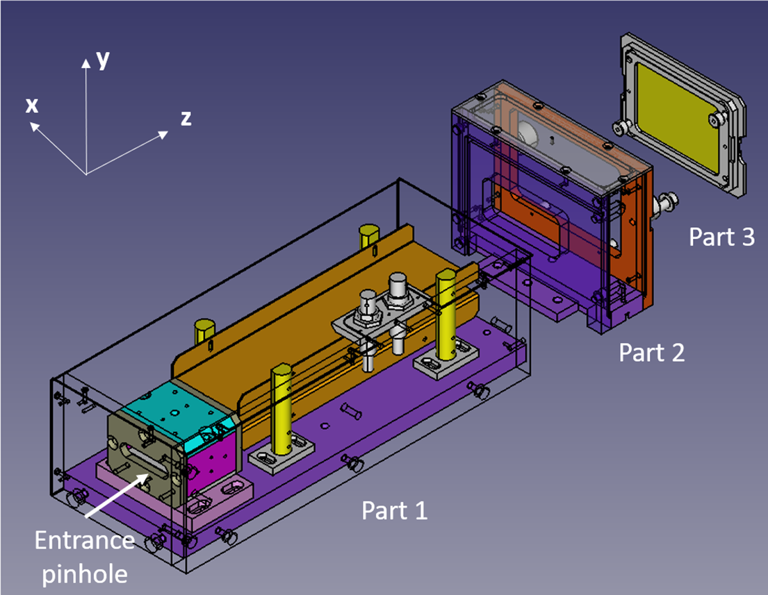

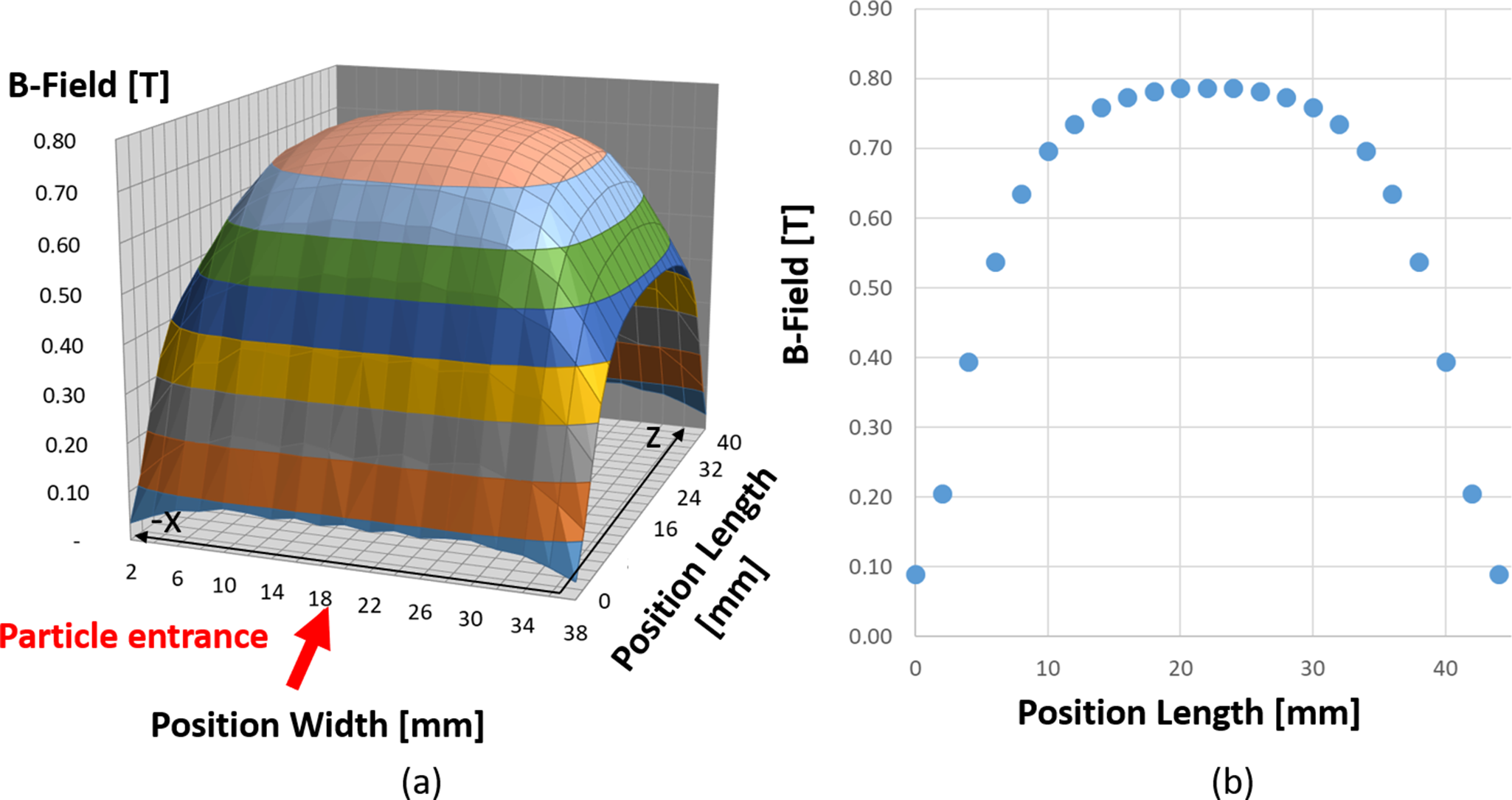


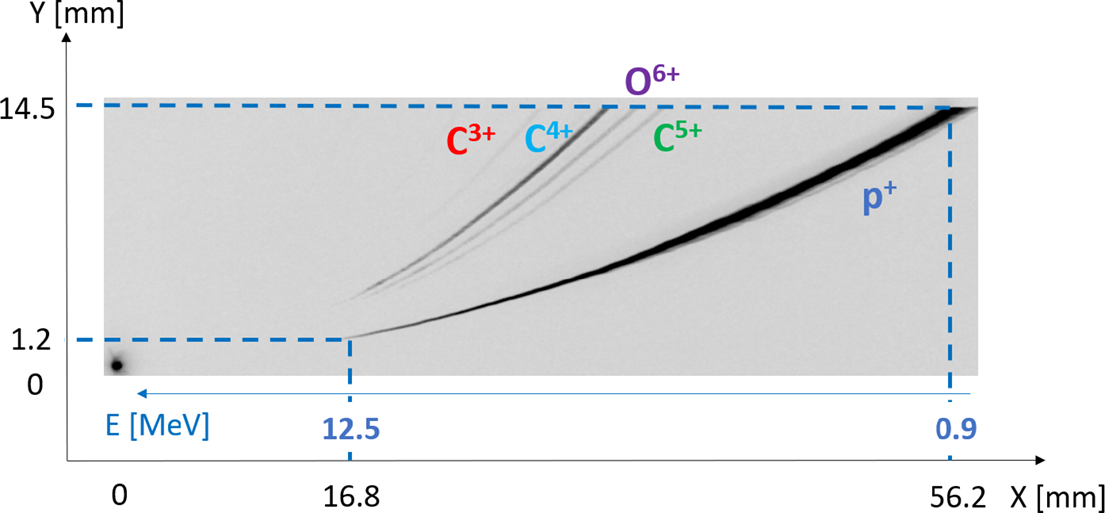


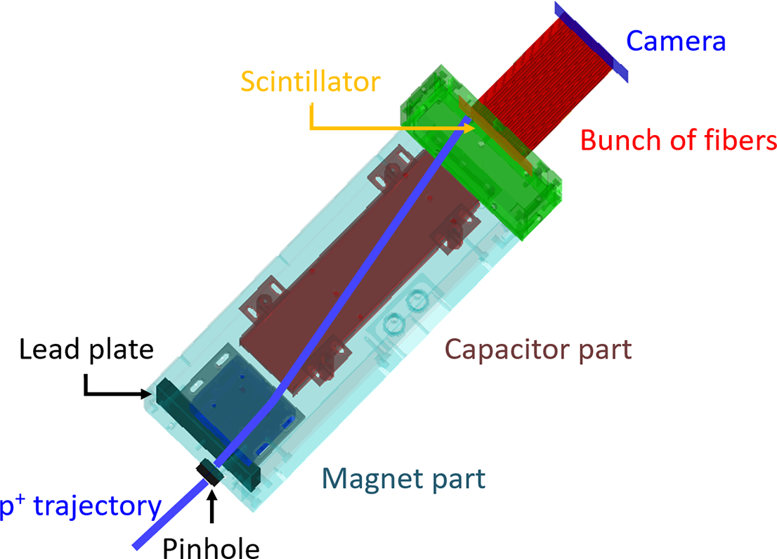
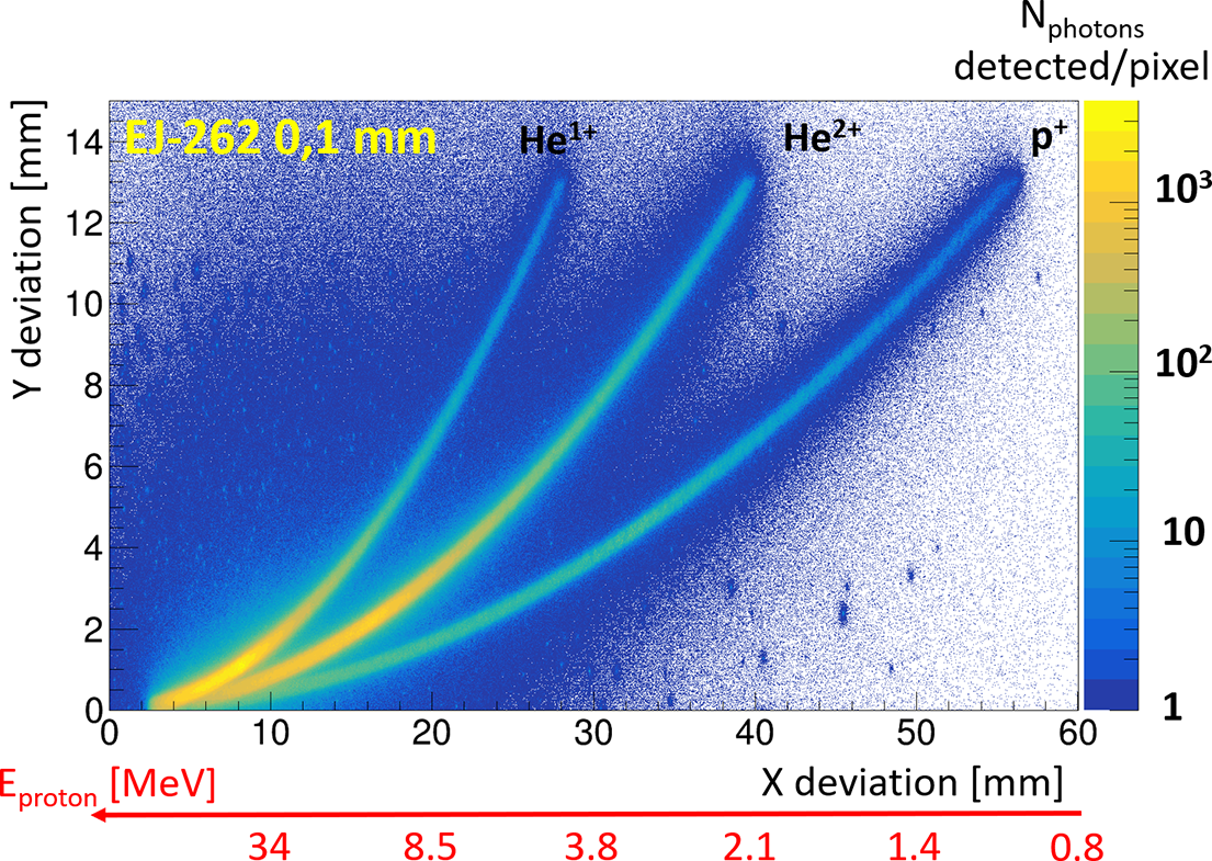


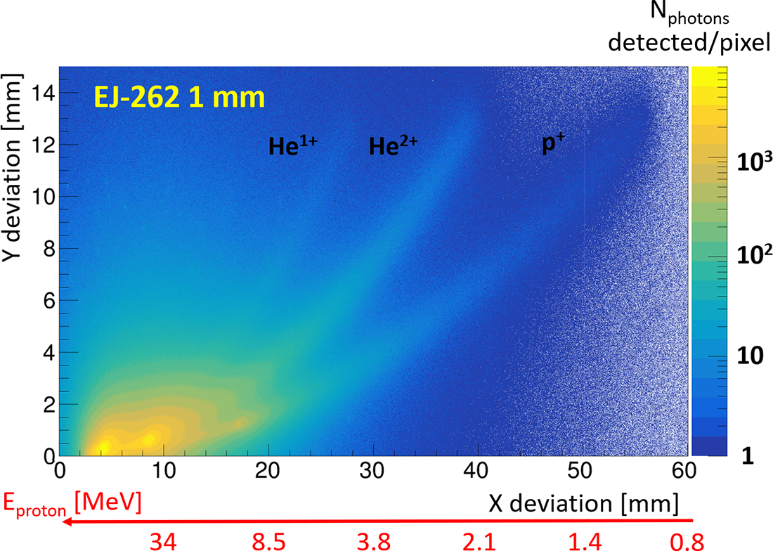


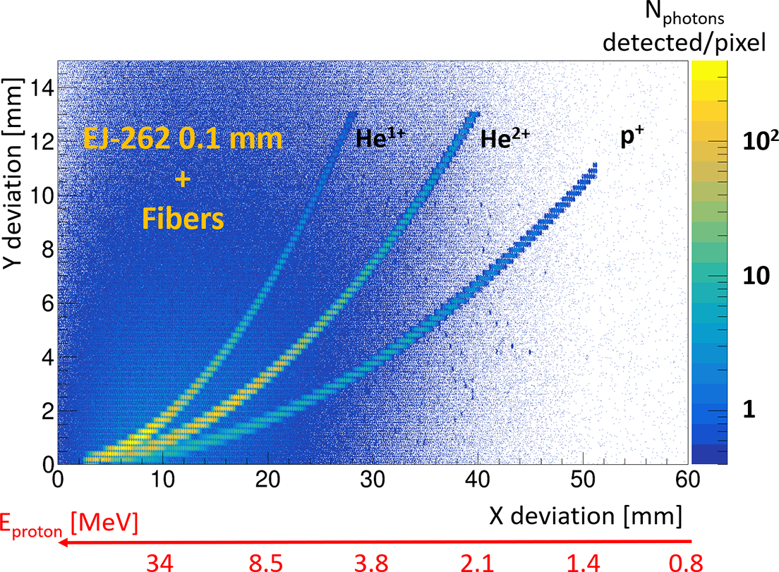


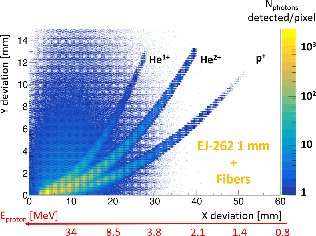


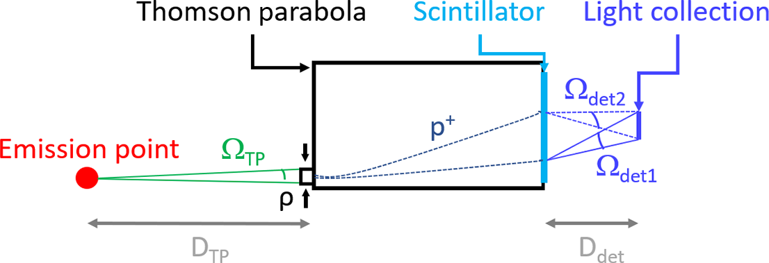


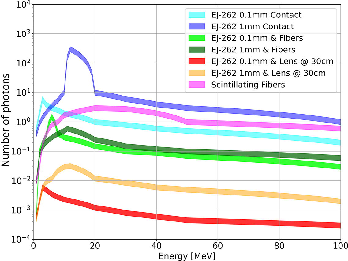

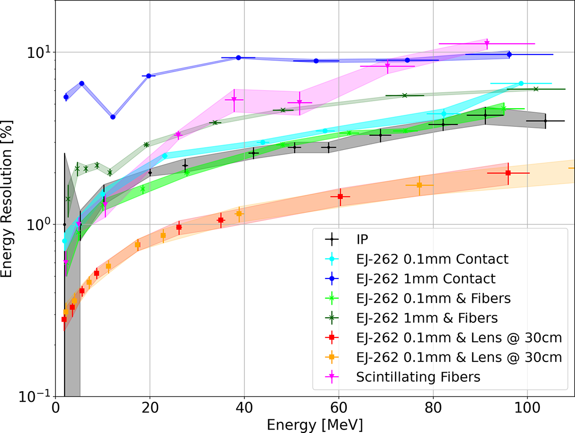

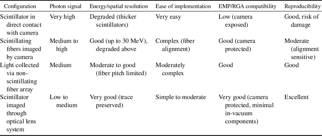
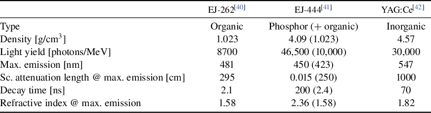

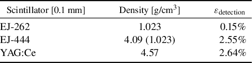


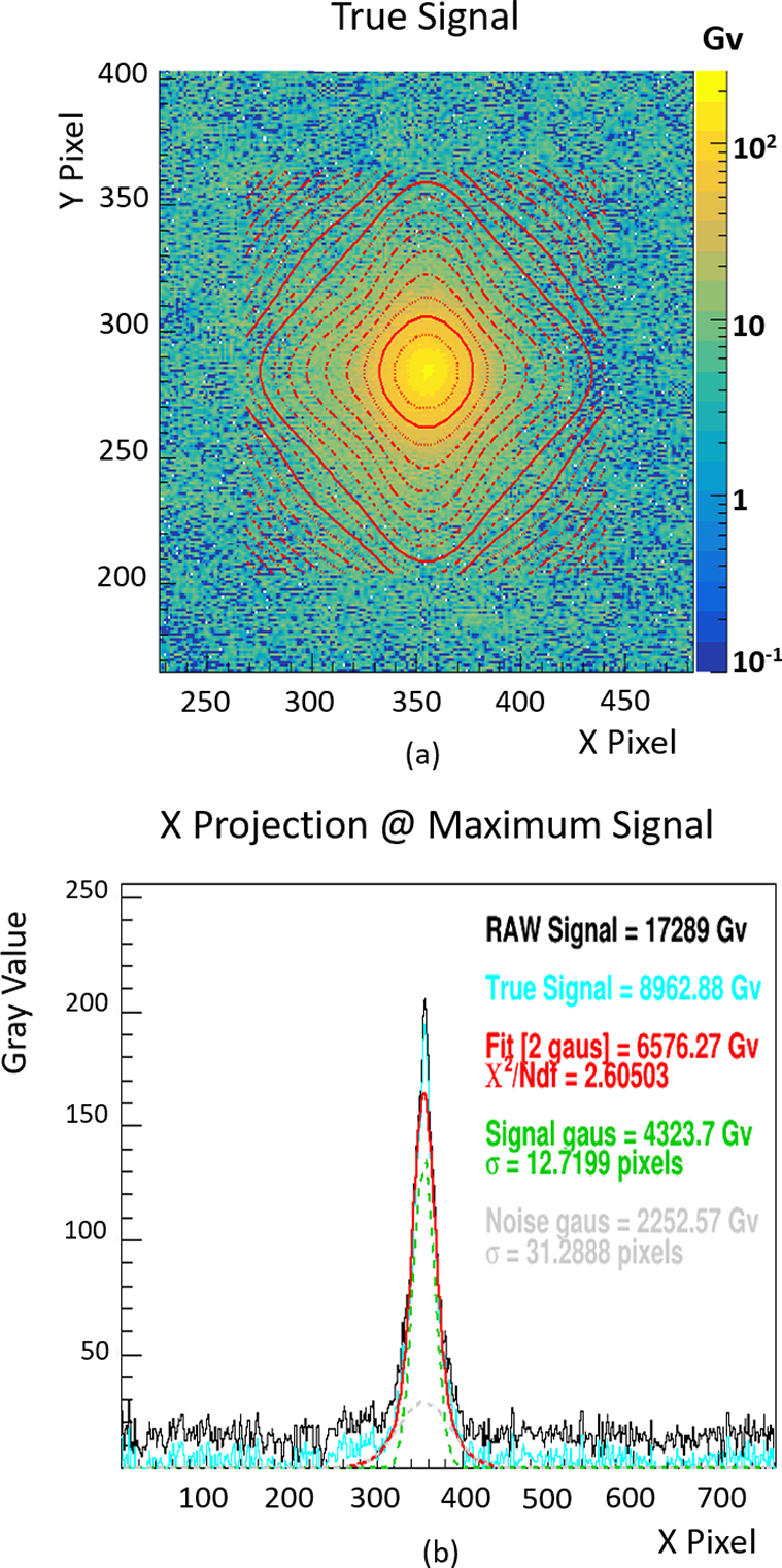
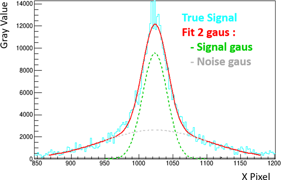

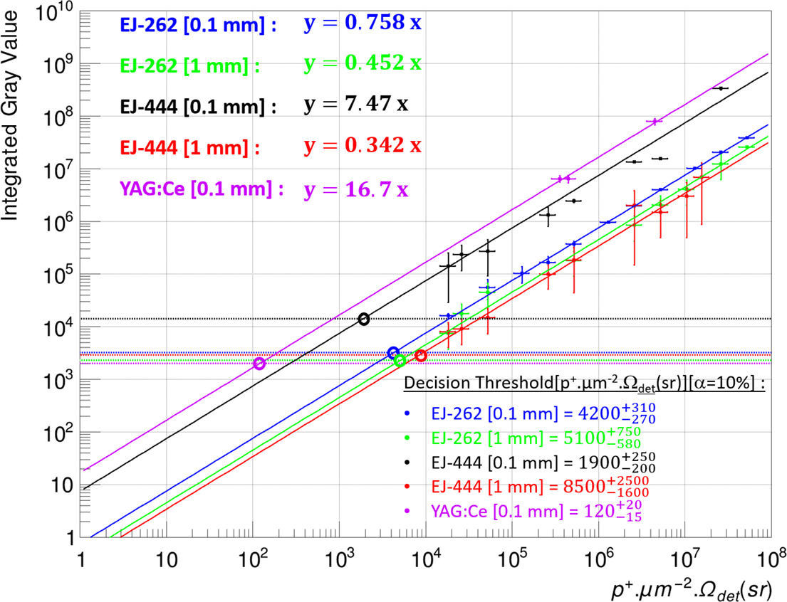


 Open access