


1. Introduction
Non-isothermal particulate flows are common and play a significant role in industries, the environment and biomedical applications, such as pollution control, pharmaceuticals, fluidised bed reactors and food processing. Heat and momentum transfer, along with their interactions with particles, can significantly alter overall system behaviour, making accurate prediction of these phenomena crucial for optimal system design. Therefore, simulation of particle-laden flows has gained more attention in recent years and led to improved models proposed, e.g. by Yu, Shao & Wachs (Reference Yu, Shao and Wachs2006), Metzger, Rahli & Yin (Reference Metzger, Rahli and Yin2013), Suzuki et al. (Reference Suzuki, Kawasaki, Furumachi, Tai and Yoshino2018), Yousefi et al. (Reference Yousefi, Ardekani, Picano and Brandt2021), Valani, Harding & Stokes (Reference Valani, Harding and Stokes2023) and Khan et al. (Reference Khan, Ali, Lee, Jang, Lee and Park2024). However, most available studies are mainly limited to spherical particles. Keeping in mind that particles have a non-spherical shape in many cases, a careful examination of such non-spherical particles will provide a better understanding of practical applications.
Near-wall regions are often dominated by high shear rates, which strongly influence particle dynamics (Shi et al. Reference Shi, Rzehak, Lucas and Magnaudet2021). The behaviour of spheroidal particles in shear flows has been extensively studied. Jeffery (Reference Jeffery1922) derived analytical solutions for the motion of a spheroidal particle in a linear shear flow at vanishing particle Reynolds numbers. He showed that the particle undergoes a periodic rotation in the so-called Jeffery orbits. However, as fluid inertia increases, the symmetry around the particle is disrupted, resulting in a more complex situation. The effect of fluid inertia on the dynamics of non-spherical particles in shear flows has been the subject of both theoretical analyses (Saffman Reference Saffman1956; Einarsson et al. Reference Einarsson, Candelier, Lundell, Angilella and Mehlig2015; Dabade, Marath & Subramanian Reference Dabade, Marath and Subramanian2016; Cui et al. Reference Cui, Liu, Qiu and Zhao2024) and experimental studies (Mason, Manley & Maass Reference Mason, Manley and Maass1956; Zettner & Yoda Reference Zettner and Yoda2001; Di Giusto et al. Reference Di Giusto, Bergougnoux, Marchioli and Guazzelli2024). Advancements in computing power have established numerical solvers as powerful tools for studying particulate flows. In this regard, rotation of finite-size spheroidal particles in shear flow can be numerically investigated by different techniques, including the lattice Boltzmann method (LBM, as performed by Aidun, Lu & Ding Reference Aidun, Lu and Ding1998; Qi & Luo Reference Qi and Luo2002; Huang et al. Reference Huang, Yang, Krafczyk and Lu2012; Rosén et al. Reference Rosén, Lundell and Aidun2014; Rosén et al. Reference Rosén, Kotsubo, Aidun, Do-Quang and Lundell2017), smoothed particle hydrodynamics (SPH, e.g. Lauricella et al. Reference Lauricella, Naderi, Zhou, Papautsky and Peng2024) and the fictitious domain method (FDM, see Yu, Phan-Thien & Tanner Reference Yu, Phan-Thien and Tanner2007). Qi & Luo (Reference Qi and Luo2002) used LBM to study the state of rotational motion of non-spherical particles in a shear flow and demonstrated that the rotational state undergoes sharp transitions with changes in Reynolds number. Huang et al. (Reference Huang, Yang, Krafczyk and Lu2012) observed that the rotational behaviour of a spheroid is sensitive not only to the Reynolds number, but also to its initial orientation. Rosén et al. (Reference Rosén, Lundell and Aidun2014) reported that as the particle Reynolds number increases, the spheroid undergoes multiple state transitions due to the competition between fluid and particle inertia. Mao & Alexeev (Reference Mao and Alexeev2014) showed that particle motion depends on the aspect ratio, particle Reynolds number, Stokes number and initial orientation. They also reported that prolate particles tend to exhibit a tumbling mode, while oblate particles favour a log-rolling mode, which was later confirmed theoretically by Cui et al. (Reference Cui, Zhao, Huang and Xu2019) and experimentally by Di Giusto et al. (Reference Di Giusto, Bergougnoux, Marchioli and Guazzelli2024).
As seen, the literature predominantly focuses on the rotational behaviour of particles in shear flows, and the role of inertia on migration trajectory has been less investigated. Fox, Schneider & Khair (Reference Fox, Schneider and Khair2021) explored the migration behaviour and final location of spherical particles in a shear flow. They demonstrated that inertia can even modify the trajectory of isotropic particles. Above a critical Reynolds number, spherical particles experience a pitchfork bifurcation in their equilibrium position. Specifically, at low particle Reynolds numbers, the particle stabilises at the centreline; but at higher Reynolds numbers, the bifurcation destabilises the central equilibrium position, leading to two new, symmetrically positioned, off-centre locations. Anand & Subramanian (Reference Anand and Subramanian2023) analytically studied the pitchfork bifurcation of point spherical particles and confirmed that beyond a critical Reynolds number, a pair of stable off-centre equilibria appear, positioned symmetrically with respect to the centreline. The location of the equilibrium position moves towards the wall by increasing the flow Reynolds number. The trajectory of spheroidal particles in shear flows has only recently been investigated by Lauricella et al. (Reference Lauricella, Naderi, Zhou, Papautsky and Peng2024); they showed that spheroidal particles can return to the centre from the off-centre positions when the particle Reynolds number is sufficiently high, whereas spherical particles become unstable at these high Reynolds numbers. Furthermore, they demonstrated the presence of comparable phenomena that have been observed in pipe flow studies by e.g. Matas et al. (Reference Matas, Morris and Guazzelli2004, Reference Matas, Morris and Guazzelli2009) and Nakayama et al. (Reference Nakayama, Yamashita, Yabu, Itano and Sugihara-Seki2019).
All these aforementioned studies are limited to isothermal cases. However, heat transfer has been shown to significantly change the behaviour and trajectory of particles in various configurations, e.g. Majlesara et al. (Reference Majlesara, Abouali, Kamali, Ardekani and Brandt2020), Fard & Khalili (Reference Fard and Khalili2022) and Wu et al. (Reference Wu, Karzhaubayev, Shen and Wang2024). To the best of our knowledge, the effect of heat transfer on the trajectory and final state of spheroidal particles in shear flows has not yet been studied. Investigating this problem and identifying the associated controlling processes could advance engineering applications and serve as the first step towards developing new techniques for separation systems of hot and active particles, particle manipulation, drug delivery, food processing and heating/cooling systems, to name only a few. For instance, Mwangi, Rizvi & Datta (Reference Mwangi, Rizvi and Datta1993) experimentally investigated, in a pioneering work, the heat transfer of particles in shear flows to study the aseptic processing of liquid foods containing a particulate phase. Shu et al. (Reference Shu, Pan, Kneer, Rietz and Rohlfs2023) investigated the effective thermal conductivity of suspensions containing oblate particles in shear flows, aiming to address the increasing demand for effective cooling systems in high-power-density electronic devices. Moreover, the manipulation of fluids and particles through thermal convection, as discussed in the works of Zhang et al. (Reference Zhang, Wang, Wang, Zhang and Wei2019) and Shen et al. (Reference Shen, Yuan, Tang, Ota, Tanaka, Hosokawa, Yalikun and Tanaka2022), has emerged as an intriguing method due to its non-invasive nature and its ability to naturally expand the range of possibilities for controlling particle motion. Deepening our understanding in this field is crucial for the further development of fundamental research and practical applications. Hence, the present study aims to thoroughly investigate the influence of heat transfer on the migration trajectory and rotational behaviour of prolate particles in shear flows. In doing so, it seeks to improve our understanding of the governing phenomena, examine the effects of various factors and analyse how different forces interact and dominate over each other. We employ a hybrid solver that combines LBM for the flow field with a finite-difference (FD) approach for the energy equation. The LBM solver relies on a modified central Hermite space collision operator, which significantly enhances accuracy and stability compared with conventional LBM techniques.
The structure of this paper is as follows. Section 2 outlines the numerical methods used in this study, including the lattice Boltzmann and immersed boundary methods. Section 3 describes the considered configuration and the relevant non-dimensional numbers. Section 4 presents simulation results of the motion of a finite-size prolate particle in shear flows by considering both isothermal and non-isothermal conditions. Finally, § 5 summarises the main findings. The validation of the computational methodology is described in Appendix A.
2. Numerical method
This section outlines the hybrid computational method employed to investigate the behaviour of particles in fluid flows and associated heat transfer processes. In this work, an enhanced central moment LBM is used to solve the momentum balance equation for incompressible flows. LBM offers significant advantages over traditional Navier–Stokes Poisson-based methods, including numerical simplicity, excellent parallelism with inherently local operations and the elimination of a Poisson solver for velocity–pressure coupling. This method has already proven effective in simulating particulate suspensions. To solve the energy equation, finite difference techniques are employed instead of a double-distribution-function LBM, offering advantages such as reduced memory consumption, enhanced stability and straightforward implementation of high-order schemes. Furthermore, the direct-force immersed boundary method (DF-IBM) is used to accurately track particle trajectories within the fluid. This advanced hybrid approach takes the benefits of both the LBM and classical computational fluid dynamics (CFD), effectively addressing the limitations associated with traditional CFD and double-distribution-function LBM.
2.1. Mass, momentum and energy balance
In this work, the flow field is modelled using the lattice Boltzmann method. The foundation of this approach lies in solving the Boltzmann equation, which describes the time evolution of density distribution functions. By discretising the Boltzmann equation in time and lattice space, we ultimately derive the now well-established ‘stream-collide’ equation for the discrete distribution function, $f_\alpha$
, represented as
$f_\alpha$
, represented as
 \begin{equation} f_{\alpha }(\textbf {x}+\textbf {e}_{\alpha }\delta t, t+\delta t)=f_{\alpha }(\textbf {x}, t)+\Omega _{\alpha }+ F_{\alpha }^{ext}. \end{equation}
In this context, $\Omega _{\alpha }$
denotes the collision operator and
$\Omega _{\alpha }$
denotes the collision operator and $F_{\alpha }^{ext}$
represents external forces. The variable
$F_{\alpha }^{ext}$
represents external forces. The variable $t$
represents the time and
$t$
represents the time and $\textbf {x}$
indicates the spatial location of the fluid node. The discrete particle velocity vectors, denoted as
$\textbf {x}$
indicates the spatial location of the fluid node. The discrete particle velocity vectors, denoted as $\textbf {e}_{\alpha }=(e_{x,\alpha },e_{y,\alpha },e_{z,\alpha })$
, are defined in (2.2) using the D3Q27 lattice stencil:
$\textbf {e}_{\alpha }=(e_{x,\alpha },e_{y,\alpha },e_{z,\alpha })$
, are defined in (2.2) using the D3Q27 lattice stencil:
 \begin{equation} \begin{matrix} e_x = [0, 1, -\!1, 0, 0, 0, 0, 1, -\!1, 1, -\!1, 1, -\!1, 1, -\!1, 0, 0, 0, 0, 1, -\!1, 1, -\!1, 1, -\!1, 1, -\!1]\\ e_y = [0, 0, 0, 1, -\!1, 0, 0, 1, 1, -\!1, -\!1, 0, 0, 0, 0, 1, -\!1, 1, -\!1, 1, 1, -\!1, -\!1, 1, 1, -\!1, -\!1]\\ e_z = [0, 0, 0, 0, 0, 1, -\!1, 0, 0, 0, 0, 1, 1, -\!1, -\!1, 1, 1, -\!1, -\!1, 1, 1, 1, 1, -\!1, -\!1, -\!1, -\!1] \end{matrix}. \end{equation}
Traditional LBM methods generally lack Galilean invariance, posing challenges for high Reynolds numbers or multiphase flows in terms of accuracy and stability (Geier, Greiner & Korvink Reference Geier, Greiner and Korvink2009; Gharibi & Ashrafizaadeh Reference Gharibi and Ashrafizaadeh2020; Gharibi et al. Reference Gharibi, Ghavaminia, Ashrafizaadeh, Zhou and Thévenin2024a ). In the current investigation, an enhanced approach is adopted, employing a modified Hermite central moments space with a collision operator featuring multiple relaxation times. The flow solver incorporates a correction term that ensures discrete Galilean invariance in the dissipation rate of shear modes at the Navier–Stokes level (Hosseini, Huang & Thévenin Reference Hosseini, Huang and Thévenin2022; Gharibi et al. Reference Gharibi, Ghavaminia, Ashrafizaadeh, Zhou and Thévenin2024b ). This method enables independent control of the bulk viscosity – an advantage not available in the conventional Hermite polynomial space. Unlike traditional formulations, this modified scheme allows for the autonomous relaxation of both trace and trace-free contributions to the second-order moments, as detailed by Hosseini et al. (Reference Hosseini, Huang and Thévenin2022). This modification enhances flexibility and precision while improving the overall robustness of LBM in capturing complex flow properties. The collision operator in this approach is expressed as
 \begin{equation} \Omega _{\alpha }=\mathcal{T}^{-1}S\mathcal{T}(f_{\alpha }^{eq}-f_{\alpha })+E_{\alpha }, \end{equation}
where the symbol $S$
stands for the diagonal tensor containing the relaxation rates, while
$S$
stands for the diagonal tensor containing the relaxation rates, while $\mathcal{T}$
represents the moments transform tensor and
$\mathcal{T}$
represents the moments transform tensor and $\mathcal{T}^{-1}$
indicates its inverse. The tensor
$\mathcal{T}^{-1}$
indicates its inverse. The tensor $\mathcal{T}$
is defined based on a set of Hermite polynomials, which are expressed as follows:
$\mathcal{T}$
is defined based on a set of Hermite polynomials, which are expressed as follows:
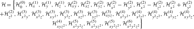 \begin{equation} \begin{matrix} \mathcal{H} = \left\{\mathcal{H}_0^{(0)}, \mathcal{H}_x^{(1)}, \mathcal{H}_y^{(1)}, \mathcal{H}_z^{(1)}, \mathcal{H}_{xy}^{(2)}, \mathcal{H}_{xz}^{(2)}, \mathcal{H}_{yz}^{(2)}, \mathcal{H}_{x^2}^{(2)}-\mathcal{H}_{y^2}^{(2)}, \mathcal{H}_{x^2}^{(2)}-\mathcal{H}_{z^2}^{(2)},\mathcal{H}_{x^2}^{(2)}+\mathcal{H}_{y^2}^{(2)}\right .\\+\mathcal{H}_{z^2}^{(2)}, \mathcal{H}_{x^2y}^{(3)}, \mathcal{H}_{x^2z}^{(3)},\mathcal{H}_{xy^2}^{(3)},\mathcal{H}_{y^2z}^{(3)}, \mathcal{H}_{xz^2}^{(3)},\mathcal{H}_{yz^2}^{(3)}, \mathcal{H}_{xyz}^{(3)}, \mathcal{H}_{x^2y^2}^{(4)}, \mathcal{H}_{x^2z^2}^{(4)}, \mathcal{H}_{y^2z^2}^{(4)}, \mathcal{H}_{x^2yz}^{(4)}, \mathcal{H}_{xy^2z}^{(4)},\\ \left . \mathcal{H}_{xyz^2}^{(4)}, \mathcal{H}_{x^2y^2z}^{(5)}, \mathcal{H}_{x^2yz^2}^{(5)}, \mathcal{H}_{xy^2z^2}^{(5)}, \mathcal{H}_{x^2y^2z^2}^{(6)} \right \} \end{matrix} \end{equation}
In (2.3), $f_{\alpha }^{eq}$
represents the equilibrium distribution, expressed through the expansion of the Maxwell–Boltzmann distribution. This expansion uses Hermite polynomials, which are orthogonal polynomials computed via a Gauss–Hermite quadrature, see Shan & He (Reference Shan and He1998)and De Rosis, Huang & Coreixas (Reference De Rosis, Huang and Coreixas2019).
$f_{\alpha }^{eq}$
represents the equilibrium distribution, expressed through the expansion of the Maxwell–Boltzmann distribution. This expansion uses Hermite polynomials, which are orthogonal polynomials computed via a Gauss–Hermite quadrature, see Shan & He (Reference Shan and He1998)and De Rosis, Huang & Coreixas (Reference De Rosis, Huang and Coreixas2019).
Unlike traditional second-order polynomial expansions of the Maxwell–Boltzmann distribution, the present approach uses a sixth-order expansion and is carefully designed to ensure the consistent preservation of Galilean invariance in the dissipation rate of shear modes. This is achieved through the term $E_{\alpha }$
, which accounts for variations in the diagonal elements of the equilibrium third-order moments (Hosseini et al. Reference Hosseini, Huang and Thévenin2022), leading to
$E_{\alpha }$
, which accounts for variations in the diagonal elements of the equilibrium third-order moments (Hosseini et al. Reference Hosseini, Huang and Thévenin2022), leading to
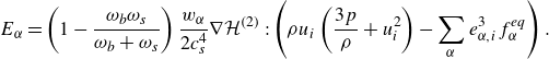 \begin{equation} E_{\alpha }=\left ( 1-\frac {\omega _{b}\omega _{s}}{\omega _{b}+\omega _{s}} \right )\frac {w_{\alpha }}{2c_{s}^{4}}\nabla \mathcal{H}^{(2)}:\left (\rho u_i\left (\frac {3p}{\rho }+u_i^2\right )-\sum _{\alpha }e_{\alpha ,i}^3 f_\alpha ^{eq} \right ). \end{equation}
Here, $p$
represents the pressure,
$p$
represents the pressure, $i$
denotes the spatial coordinate,
$i$
denotes the spatial coordinate, $\omega _{s}$
signifies the shear relaxation frequency and
$\omega _{s}$
signifies the shear relaxation frequency and $\omega _{b}$
corresponds to the relaxation frequency associated with bulk viscosity, which is set to 1.0. The transformation tensor
$\omega _{b}$
corresponds to the relaxation frequency associated with bulk viscosity, which is set to 1.0. The transformation tensor $\mathcal{T}$
, constructed from modified central Hermite polynomials, is defined as follows:
$\mathcal{T}$
, constructed from modified central Hermite polynomials, is defined as follows:
 \begin{equation} \mathcal{T}=[|\overline {\mathcal{T}}_{0}\rangle ,\ldots ,\overline {\mathcal{T}}_{26}\rangle ], \end{equation}
where column vectors $|\overline {\mathcal{T}}_{\alpha }\rangle$
corresponds to the D3Q27 stencil based on Hermite polynomials, using the shifted velocity vector
$|\overline {\mathcal{T}}_{\alpha }\rangle$
corresponds to the D3Q27 stencil based on Hermite polynomials, using the shifted velocity vector $\overline {\textbf {e}}_{\alpha }=\textbf {e}_{\alpha }-\textbf {u}$
. The diagonal tensor of relaxation rates, denoted as
$\overline {\textbf {e}}_{\alpha }=\textbf {e}_{\alpha }-\textbf {u}$
. The diagonal tensor of relaxation rates, denoted as $S$
for the D3Q27 stencil, is given by
$S$
for the D3Q27 stencil, is given by
 \begin{equation} S=\hbox{diag}(1,1,1,1,\omega _{s},\omega _{s},\omega _{s},\omega _{s},\omega _{s},\omega _{b},\omega _{a},\ldots ,\omega _{a}), \end{equation}
where $\omega _{a}$
is an arbitrary frequency that is set to 1.0 in this study. Macroscopic properties such as density
$\omega _{a}$
is an arbitrary frequency that is set to 1.0 in this study. Macroscopic properties such as density $\rho$
, velocity
$\rho$
, velocity $\textbf {u}$
and pressure
$\textbf {u}$
and pressure $p$
are derived from the following equations:
$p$
are derived from the following equations:
 \begin{align}&\,\,\,\, \rho =\sum _{\alpha }f_\alpha , \end{align}
 \begin{align}& \rho \textbf {u}=\sum _{\alpha } e_\alpha f_\alpha , \end{align}
 \begin{align}&\quad\, p=\rho c_s^2. \end{align}
For incompressible flows with variable properties, the energy equation simplifies by ignoring the effects of viscous heating to
 \begin{equation} \frac {\partial (\rho C_p T)}{\partial t}+\nabla .(\textbf {u}\ \rho C_pT)=\nabla .(k\nabla T)+ Q. \end{equation}
Here, $k$
represents thermal conductivity,
$k$
represents thermal conductivity, $Q$
is the heat source term,
$Q$
is the heat source term, $T$
denotes temperature and
$T$
denotes temperature and $C_p$
is the specific heat capacity. This energy equation is solved using a finite-difference technique. For the advection term, we apply a third-order weighted essentially non-oscillatory (WENO) method, while diffusion is handled with a fourth-order central FD scheme, ensuring stability and accuracy throughout the computations. The method is implemented in a fully explicit formulation as shown by Gharibi et al. (Reference Gharibi, Ghavaminia, Ashrafizaadeh, Zhou and Thévenin2024b
). To couple the energy solver to the lattice Boltzmann solver, the term for the buoyancy force (
$C_p$
is the specific heat capacity. This energy equation is solved using a finite-difference technique. For the advection term, we apply a third-order weighted essentially non-oscillatory (WENO) method, while diffusion is handled with a fourth-order central FD scheme, ensuring stability and accuracy throughout the computations. The method is implemented in a fully explicit formulation as shown by Gharibi et al. (Reference Gharibi, Ghavaminia, Ashrafizaadeh, Zhou and Thévenin2024b
). To couple the energy solver to the lattice Boltzmann solver, the term for the buoyancy force ( $\textbf {F}_{B}$
) within the flow-field is computed using the Boussinesq approximation, as expressed in (2.12), and is implemented as an external force in (2.1),
$\textbf {F}_{B}$
) within the flow-field is computed using the Boussinesq approximation, as expressed in (2.12), and is implemented as an external force in (2.1),
 \begin{equation} \textbf {F}_{B}=\rho _{f,0}\textbf {g}\beta (T-T_{0}), \end{equation}
where $T_{0}$
is the reference temperature,
$T_{0}$
is the reference temperature, $\textbf {g}$
is the gravitational acceleration,
$\textbf {g}$
is the gravitational acceleration, $\rho _{f,0}$
is the fluid density at the specified reference temperature and
$\rho _{f,0}$
is the fluid density at the specified reference temperature and $\beta$
is the thermal expansion coefficient of the fluid.
$\beta$
is the thermal expansion coefficient of the fluid.
2.2. Immersed boundary method
The direct-forcing and direct-heating IBM is used in this work to implement fluid–particle interaction. In this method, at each Lagrangian node, the force term, $\textbf {F}_{l}$
, and the heat source term,
$\textbf {F}_{l}$
, and the heat source term, $Q_l$
, are calculated using
$Q_l$
, are calculated using
 \begin{align}&\,\, \textbf {F}_{l}=\frac {\textbf {u}^{d}-\textbf {u}^{noF}}{\Delta t}, \end{align}
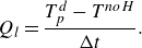 \begin{align}& Q_{l}=\frac {T_{p}^{d}-T^{noH}}{\Delta t}. \end{align}
where $\textbf {u}^{d}$
is the desired velocity vector,
$\textbf {u}^{d}$
is the desired velocity vector, $T$
is the temperature and
$T$
is the temperature and $\Delta t$
is the time step. The subscripts
$\Delta t$
is the time step. The subscripts $l$
indicate Lagrangian points. The quantities
$l$
indicate Lagrangian points. The quantities
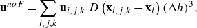
 $\textbf {u}^{noF}$
and
$\textbf {u}^{noF}$
and
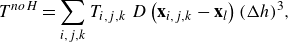
 $T^{noH}$
are calculated based on the values at Eulerian nodes using discrete Delta functions:
$T^{noH}$
are calculated based on the values at Eulerian nodes using discrete Delta functions:
 \begin{align}&\, \textbf {u}^{noF}=\sum _{i,j,k} \textbf {u}_{i,j,k}\ D\left ( \textbf {x}_{i,j,k}-\textbf {x}_{l} \right ) (\Delta h)^{3}, \end{align}
 \begin{align}& T^{noH}=\sum _{i,j,k} T_{i,j,k}\ D\left ( \textbf {x}_{i,j,k}-\textbf {x}_{l} \right ) (\Delta h)^{3}, \end{align}
where the subscripts $i,j,k$
denote the Eulerian nodes,
$i,j,k$
denote the Eulerian nodes, $\textbf {x}$
represents the position,
$\textbf {x}$
represents the position, $\Delta h$
denotes the lattice size and
$\Delta h$
denotes the lattice size and $D$
is the Dirac delta function, which uses the 4-point delta function proposed by Peskin (Reference Peskin2002). The desired velocity
$D$
is the Dirac delta function, which uses the 4-point delta function proposed by Peskin (Reference Peskin2002). The desired velocity
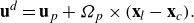
 $\textbf {u}^d$
is calculated using
$\textbf {u}^d$
is calculated using
 \begin{equation} \textbf {u}^{d}=\textbf {u}_{p}+\Omega _{p}\times (\textbf {x}_{l}-\textbf {x}_{c}). \end{equation}
Here, the subscript $p$
denotes the particle, the subscript
$p$
denotes the particle, the subscript $c$
represents the centre of the particle and
$c$
represents the centre of the particle and $\Omega _{p}$
is the particle’s angular velocity. The particle translational velocity
$\Omega _{p}$
is the particle’s angular velocity. The particle translational velocity $\textbf {u}_{p}$
and angular velocity
$\textbf {u}_{p}$
and angular velocity $\Omega _{p}$
are calculated at each time step using the fundamental laws of motion, based on the method proposed by Feng & Michaelides (Reference Feng and Michaelides2009) and Eshghinejadfard et al. (Reference Eshghinejadfard, Abdelsamie, Janiga and Thévenin2016). The temperature of the Lagrangian (particle) nodes is determined by the method outlined by Gharibi et al. (Reference Gharibi, Ghavaminia, Ashrafizaadeh, Zhou and Thévenin2024b
). Finally, the interaction force and interaction heat source are applied to the Eulerian nodes using the following equations:
$\Omega _{p}$
are calculated at each time step using the fundamental laws of motion, based on the method proposed by Feng & Michaelides (Reference Feng and Michaelides2009) and Eshghinejadfard et al. (Reference Eshghinejadfard, Abdelsamie, Janiga and Thévenin2016). The temperature of the Lagrangian (particle) nodes is determined by the method outlined by Gharibi et al. (Reference Gharibi, Ghavaminia, Ashrafizaadeh, Zhou and Thévenin2024b
). Finally, the interaction force and interaction heat source are applied to the Eulerian nodes using the following equations:
 \begin{align}&\quad \textbf {F}_{i,j,k}=\rho _f \sum _{l}\textbf {F}_{l}\ D\left ( \textbf {x}_{i,j,k}-\textbf {x}_{l} \right )\ \Delta V_{l}, \end{align}
 \begin{align}& Q_{i,j,k}=\rho _f C_{p,f}\sum _{l}Q_{l}\ D\left ( \textbf {x}_{i,j,k}-\textbf {x}_{l} \right )\ \Delta V_{l}, \end{align}
where $\Delta V_{l}$
represents the unit volume of the relevant Lagrangian boundary point segment, and the subscript
$\Delta V_{l}$
represents the unit volume of the relevant Lagrangian boundary point segment, and the subscript $f$
denotes the fluid. The interaction force is applied as an external force in the LBM solver, while the heat source is treated as a source term in the energy equation to model fluid–solid interactions. The IBM method and the hybrid solver for energy and fluid flow are detailed further by Gharibi et al. (Reference Gharibi, Ghavaminia, Ashrafizaadeh, Zhou and Thévenin2024b
).
$f$
denotes the fluid. The interaction force is applied as an external force in the LBM solver, while the heat source is treated as a source term in the energy equation to model fluid–solid interactions. The IBM method and the hybrid solver for energy and fluid flow are detailed further by Gharibi et al. (Reference Gharibi, Ghavaminia, Ashrafizaadeh, Zhou and Thévenin2024b
).
3. Geometric configuration and non-dimensional parameters
For the test cases, various non-dimensional parameters and characteristic scales are employed to describe particle dynamics, thermal behaviour and fluid flow characteristics. This section defines the key non-dimensional parameters and outlines the geometric configuration used in the simulations.
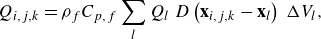
In this study, the fluid flow between two moving parallel plates that move with velocity $u_0$
in opposite directions is considered, as shown in figure 1. The distance between the plates is
$u_0$
in opposite directions is considered, as shown in figure 1. The distance between the plates is $H$
. The domain size is set to
$H$
. The domain size is set to $2H\times H\times H$
, where the length in the flow direction is twice that of the other dimensions, as proposed by Fox et al. (Reference Fox, Schneider and Khair2021). A no-slip boundary condition is imposed on the moving wall boundaries, while periodic boundary conditions are applied in the other directions. A particle, initially located at
$2H\times H\times H$
, where the length in the flow direction is twice that of the other dimensions, as proposed by Fox et al. (Reference Fox, Schneider and Khair2021). A no-slip boundary condition is imposed on the moving wall boundaries, while periodic boundary conditions are applied in the other directions. A particle, initially located at $(x_0,y_0,z_0)$
, is considered within the domain. We will investigate both spherical and spheroidal particles. In the case of the spherical particle, the radius of the particle is
$(x_0,y_0,z_0)$
, is considered within the domain. We will investigate both spherical and spheroidal particles. In the case of the spherical particle, the radius of the particle is $r_p$
, whereas, for a spheroidal particle, the polar (major) radius is
$r_p$
, whereas, for a spheroidal particle, the polar (major) radius is $a$
and the equatorial (minor) radius is
$a$
and the equatorial (minor) radius is $b$
, and the aspect ratio
$b$
, and the aspect ratio $r$
is defined as
$r$
is defined as $r=a/b$
. The confinement ratio for the spherical particle is
$r=a/b$
. The confinement ratio for the spherical particle is $K = {r_p}/{H}$
and in the case of a spheroidal particle, is defined as
$K = {r_p}/{H}$
and in the case of a spheroidal particle, is defined as $K = {a}/{H}$
. The global coordinate system used to define the position
$K = {a}/{H}$
. The global coordinate system used to define the position $(x,y,z)$
and orientation of the prolate spheroid is shown in figure 2.
$(x,y,z)$
and orientation of the prolate spheroid is shown in figure 2.
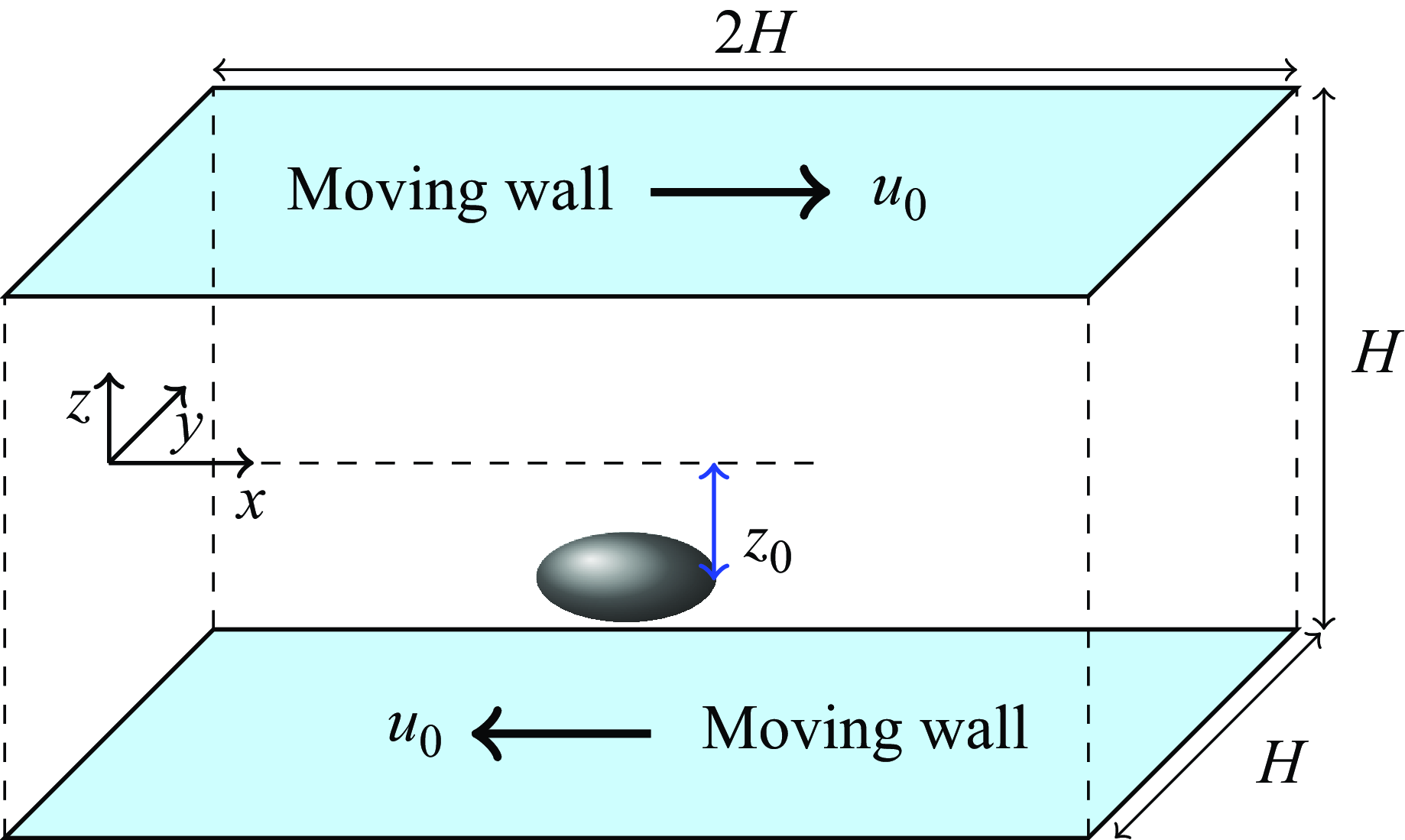
Figure 1. Schematic of the simulation domain for a Couette flow between two parallel plates moving in opposite directions.
Figure 2. Global coordinate system used to define the position ( $x,y,z$
) and orientation of a prolate spheroid.
$x,y,z$
) and orientation of a prolate spheroid.
The shear rate in this geometry is calculated as
 \begin{equation} G = {2 u_0}/{H}. \end{equation}
In this study, the normalised values are indicated by a superscript $^*$
and the characteristic length
$^*$
and the characteristic length $H$
is used for length normalisation, such as
$H$
is used for length normalisation, such as $z_0^*= z_0/H$
, and
$z_0^*= z_0/H$
, and $1/G$
is employed for time normalisation, as illustrated by
$1/G$
is employed for time normalisation, as illustrated by $t^* = tG$
. The particle Reynolds number is defined for the spherical particle as
$t^* = tG$
. The particle Reynolds number is defined for the spherical particle as
 \begin{equation} \textit{Re}_p = {G r_p^2}/{\nu }, \end{equation}
whereas for a spheroidal particle, it is given by
 \begin{equation} \textit{Re}_p = {G a^2}/{\nu }, \end{equation}
where $\nu$
is the dynamic viscosity of the fluid. The density ratio between the particle and the fluid is defined as
$\nu$
is the dynamic viscosity of the fluid. The density ratio between the particle and the fluid is defined as
 \begin{equation} \rho _r=\rho _p/\rho _f, \end{equation}
where the subscripts $p$
and
$p$
and $f$
denote the particle and fluid, respectively.
$f$
denote the particle and fluid, respectively.
In the analysis of heat transfer, the key non-dimensional parameters that characterise thermal behaviour are as follows. The specific heat capacity ratio is defined as
 \begin{equation} C_{p,r} = \frac {C_{p,p}}{C_{p,f}}. \end{equation}
The non-dimensional temperature is expressed as
 \begin{equation} T^* = \frac {T - T_{0,f}}{|\Delta T_0|}, \end{equation}
where $T_{0,f}$
represents the initial temperature of the surrounding fluid and
$T_{0,f}$
represents the initial temperature of the surrounding fluid and $\Delta T_0$
is the initial solid–fluid temperature difference. The Prandtl number, which describes the ratio of momentum diffusivity to thermal diffusivity, is given by
$\Delta T_0$
is the initial solid–fluid temperature difference. The Prandtl number, which describes the ratio of momentum diffusivity to thermal diffusivity, is given by
 \begin{equation} {Pr}= \frac {\rho _f \nu C_{p,f}}{k_f}. \end{equation}
Finally, the Grashof number, representing the ratio of buoyancy forces to viscous forces, is defined as
 \begin{equation} {Gr}=\frac {\rho _{f}^2\ g\ \beta \ D_p^3\Delta T}{\mu ^2}, \end{equation}
where $\mu$
is the kinematic viscosity of the fluid,
$\mu$
is the kinematic viscosity of the fluid, $D_p=2r_p$
for a spherical particle and
$D_p=2r_p$
for a spherical particle and $D_p=2a$
for a spheroidal particle.
$D_p=2a$
for a spheroidal particle.
4. Results and discussion
After thoroughly validating different scenarios for spheres, spheroids, isothermal and non-isothermal cases, as presented in Appendix A in the interest of space, we now investigate the behaviour of spheroidal particles in shear flows between two parallel walls including thermal effects. In particular, we will concentrate on non-isothermal cases, since those have not been explored in detail in previously published investigations.
4.1. Isothermal neutrally buoyant prolate particle in shear flow
In this test case, the prolate particle is moving and rotating in an isothermal shear flow and is characterised by a polar (major) radius $a$
and an equatorial (minor) radius
$a$
and an equatorial (minor) radius $b$
, and an aspect ratio of
$b$
, and an aspect ratio of $r= 2$
. A confinement ratio of
$r= 2$
. A confinement ratio of $K= 0.2$
is considered. The density ratio between the particle and the fluid is equal to
$K= 0.2$
is considered. The density ratio between the particle and the fluid is equal to $\rho _r=\rho _p/\rho _f=1.0$
(neutrally buoyant particle). The computational domain and its set-up are consistent with the configuration shown in figure 1. A grid size of
$\rho _r=\rho _p/\rho _f=1.0$
(neutrally buoyant particle). The computational domain and its set-up are consistent with the configuration shown in figure 1. A grid size of $N_x \times N_y \times N_z = 240 \times 120 \times 120$
is used for
$N_x \times N_y \times N_z = 240 \times 120 \times 120$
is used for $\textit{Re}_P \lt 10$
. For
$\textit{Re}_P \lt 10$
. For $10 \leqslant \text{Re}_P \lt 120$
, a grid size of
$10 \leqslant \text{Re}_P \lt 120$
, a grid size of $N_x \times N_y \times N_z = 512 \times 256 \times 256$
is employed and for
$N_x \times N_y \times N_z = 512 \times 256 \times 256$
is employed and for $\text{Re}_P \geqslant 120$
, a grid size of
$\text{Re}_P \geqslant 120$
, a grid size of $N_x \times N_y \times N_z = 770 \times 385 \times 385$
is used.
$N_x \times N_y \times N_z = 770 \times 385 \times 385$
is used.
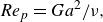
Figure 3. Migration trajectory of an isothermal prolate particle ( $z/H$
) in a Couette flow versus dimensionless time (
$z/H$
) in a Couette flow versus dimensionless time ( $Gt$
) at various Reynolds numbers (
$Gt$
) at various Reynolds numbers ( $\textit{Re}_p$
).
$\textit{Re}_p$
).
In the first case, the particle centre is initially positioned at $(x,y,z)=(H,0,-0.1H)$
, with its polar (major) radius aligned in the
$(x,y,z)=(H,0,-0.1H)$
, with its polar (major) radius aligned in the $x$
-direction, i.e.
$x$
-direction, i.e. $(\theta ,\phi )=(\pi /2,0)$
. The particle is released from a stationary situation and starts experiencing both rotation and translation. Figure 3 shows the particle migration trajectory represented by its normalised transverse position (
$(\theta ,\phi )=(\pi /2,0)$
. The particle is released from a stationary situation and starts experiencing both rotation and translation. Figure 3 shows the particle migration trajectory represented by its normalised transverse position ( $z/H$
) versus non-dimensional time (
$z/H$
) versus non-dimensional time ( $Gt$
) at various Reynolds numbers. It is seen that at low Reynolds numbers (
$Gt$
) at various Reynolds numbers. It is seen that at low Reynolds numbers ( $\textit{Re}_p= 3$
), the final equilibrium position is at the centre of the domain (i.e.
$\textit{Re}_p= 3$
), the final equilibrium position is at the centre of the domain (i.e. $z/H=0$
), similar to the behaviour observed for spheres by Fox et al. (Reference Fox, Schneider and Khair2021). However, as the Reynolds number increases beyond
$z/H=0$
), similar to the behaviour observed for spheres by Fox et al. (Reference Fox, Schneider and Khair2021). However, as the Reynolds number increases beyond $\textit{Re}_p= 3$
, new stable but off-centre equilibrium positions emerge and the final particle location becomes dependent on the Reynolds number. Our simulations showed that at
$\textit{Re}_p= 3$
, new stable but off-centre equilibrium positions emerge and the final particle location becomes dependent on the Reynolds number. Our simulations showed that at $\textit{Re}_p \approx 6$
and beyond, a pitchfork bifurcation occurs; i.e. at this point, the final equilibrium position of the particle can be either in the lower or upper half of the channel, depending on its initial position. We call this point the ‘first critical Reynolds number’. Notably, the particle did not take an equilibrium position below
$\textit{Re}_p \approx 6$
and beyond, a pitchfork bifurcation occurs; i.e. at this point, the final equilibrium position of the particle can be either in the lower or upper half of the channel, depending on its initial position. We call this point the ‘first critical Reynolds number’. Notably, the particle did not take an equilibrium position below $z/H\approx -0.29$
in the simulations, which is the final position observed at
$z/H\approx -0.29$
in the simulations, which is the final position observed at $\textit{Re}_p=60$
and
$\textit{Re}_p=60$
and $100$
. Nevertheless, in all cases from
$100$
. Nevertheless, in all cases from $\textit{Re}_p= 6$
up to
$\textit{Re}_p= 6$
up to $\textit{Re}_p= 120$
, the particle ends up in the lower half of the domain. Beyond this point, specifically for
$\textit{Re}_p= 120$
, the particle ends up in the lower half of the domain. Beyond this point, specifically for $\textit{Re}_p= 140$
, the equilibrium position suddenly shifts upwards, bringing the prolate particle back towards the centre (second critical Reynolds number), thereby corroborating the findings of Lauricella et al. (Reference Lauricella, Naderi, Zhou, Papautsky and Peng2024). However, the value of this second critical Reynolds number differs from that reported by Lauricella et al. (Reference Lauricella, Naderi, Zhou, Papautsky and Peng2024). In our study, the particle returns to the centre at
$\textit{Re}_p= 140$
, the equilibrium position suddenly shifts upwards, bringing the prolate particle back towards the centre (second critical Reynolds number), thereby corroborating the findings of Lauricella et al. (Reference Lauricella, Naderi, Zhou, Papautsky and Peng2024). However, the value of this second critical Reynolds number differs from that reported by Lauricella et al. (Reference Lauricella, Naderi, Zhou, Papautsky and Peng2024). In our study, the particle returns to the centre at $\textit{Re}_p = 140$
, whereas Lauricella et al. (Reference Lauricella, Naderi, Zhou, Papautsky and Peng2024) stated that this had already occurred at
$\textit{Re}_p = 140$
, whereas Lauricella et al. (Reference Lauricella, Naderi, Zhou, Papautsky and Peng2024) stated that this had already occurred at $\textit{Re}_p = 90$
. This difference may stem from the very different numerical description coming with SPH. Additionally, to illustrate the potential effects of under-resolution, we present in figure 4 a comparison of results from both coarse and fine grids using our LBM solver (ALBORZ) alongside those from Lauricella et al. (Reference Lauricella, Naderi, Zhou, Papautsky and Peng2024). It is seen that for the coarse mesh, our simulations also show that the particle would return to the centre at
$\textit{Re}_p = 90$
. This difference may stem from the very different numerical description coming with SPH. Additionally, to illustrate the potential effects of under-resolution, we present in figure 4 a comparison of results from both coarse and fine grids using our LBM solver (ALBORZ) alongside those from Lauricella et al. (Reference Lauricella, Naderi, Zhou, Papautsky and Peng2024). It is seen that for the coarse mesh, our simulations also show that the particle would return to the centre at $\textit{Re}_p = 90$
, while refining the mesh would delay the transition to higher Reynolds numbers. This indicates that resolution may strongly influence the particle behaviour and impact the final equilibrium position, as also shown in Appendix A.
$\textit{Re}_p = 90$
, while refining the mesh would delay the transition to higher Reynolds numbers. This indicates that resolution may strongly influence the particle behaviour and impact the final equilibrium position, as also shown in Appendix A.

Figure 4. Effect of grid resolution on the migration trajectory of an isothermal prolate particle at $\textit{Re}_p=90$
and initial orientation of
$\textit{Re}_p=90$
and initial orientation of $(\theta , \phi ) = (\pi /2, \pi /2)$
compared with the result of Lauricella et al. (Reference Lauricella, Naderi, Zhou, Papautsky and Peng2024).
$(\theta , \phi ) = (\pi /2, \pi /2)$
compared with the result of Lauricella et al. (Reference Lauricella, Naderi, Zhou, Papautsky and Peng2024).
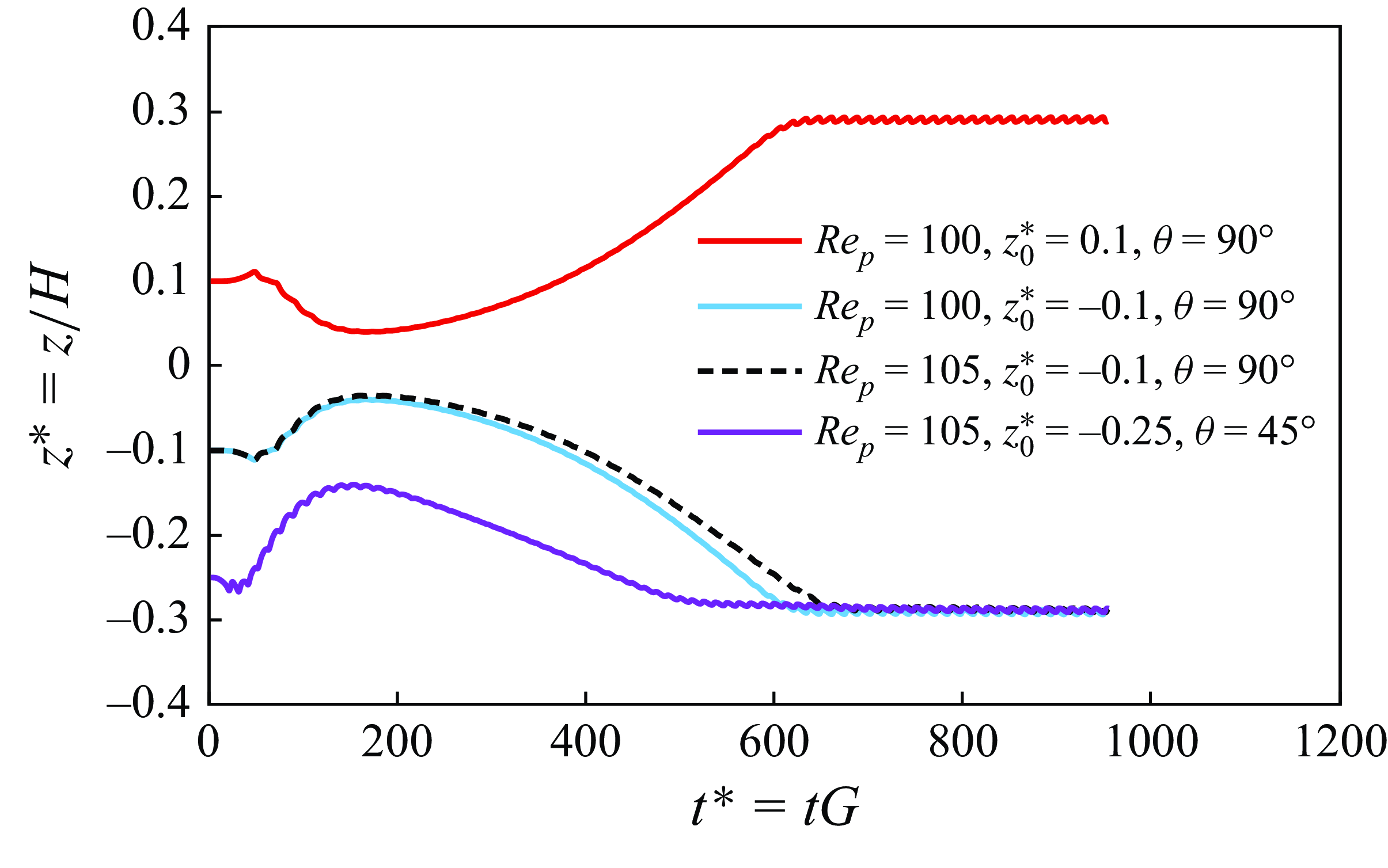
Figure 5. Influence of initial position and orientation on the final equilibrium position of an isothermal prolate particle.
To further investigate the pitchfork bifurcation phenomenon, the prolate particle is then placed at two symmetric off-centre locations, i.e. either $ z^* = +0.1$
or
$ z^* = +0.1$
or $ z^* = -0.1$
for
$ z^* = -0.1$
for $\textit{Re}_p=100$
. As shown in figure 5, the particle migrates to two distinct symmetric equilibrium positions on either side of the centreline depending on its initial location. If the particle starts in the lower half of the domain, its final equilibrium position will also be in the lower half, and vice versa.
$\textit{Re}_p=100$
. As shown in figure 5, the particle migrates to two distinct symmetric equilibrium positions on either side of the centreline depending on its initial location. If the particle starts in the lower half of the domain, its final equilibrium position will also be in the lower half, and vice versa.
Next, the influence of the initial position and orientation of the particle on its final location is further examined in figure 5. At $\textit{Re}_p = 105$
, two initial configurations of
$\textit{Re}_p = 105$
, two initial configurations of $z^*_0=-0.1, \theta =\pi /2$
and
$z^*_0=-0.1, \theta =\pi /2$
and $z^*_0=-0.25, \theta =\pi /4$
are separately tested. It is observed that the particle’s initial position and orientation do not affect its final equilibrium position, at least as long as the particle starts in the
$z^*_0=-0.25, \theta =\pi /4$
are separately tested. It is observed that the particle’s initial position and orientation do not affect its final equilibrium position, at least as long as the particle starts in the $x{-}z$
plane and is released in the lower half of the channel. In both cases, the particle settles at
$x{-}z$
plane and is released in the lower half of the channel. In both cases, the particle settles at $z^* \approx -0.29$
regardless of its initial location or orientation. This confirms that the Reynolds number, which quantifies particle inertia, is the dominant factor determining the final equilibrium position. While initial orientation or location may strongly influence the particle trajectory, they do not impact its final position. However, if the particle is released once in the lower and once in the upper half, the pitchfork bifurcation occurs as illustrated earlier in figure 5.
$z^* \approx -0.29$
regardless of its initial location or orientation. This confirms that the Reynolds number, which quantifies particle inertia, is the dominant factor determining the final equilibrium position. While initial orientation or location may strongly influence the particle trajectory, they do not impact its final position. However, if the particle is released once in the lower and once in the upper half, the pitchfork bifurcation occurs as illustrated earlier in figure 5.
4.2. Hot negatively buoyant prolate particle in shear flow
In this section, the behaviour of a hot prolate particle in the shear flow between two parallel plates is examined. The particle aspect ratio is $r= 2$
and a confinement ratio of
$r= 2$
and a confinement ratio of $K = 0.2$
is considered in all simulations. To investigate the heat transfer effect, the particle is assumed to be hot with a constant non-dimensional temperature of
$K = 0.2$
is considered in all simulations. To investigate the heat transfer effect, the particle is assumed to be hot with a constant non-dimensional temperature of $T^*_p= {(T - T_{0,f})}/{|\Delta T_0|}=1$
. The Prandtl number of the fluid is set to
$T^*_p= {(T - T_{0,f})}/{|\Delta T_0|}=1$
. The Prandtl number of the fluid is set to ${Pr}=6.9$
(representing water at ambient temperature), with the ratio of heat capacities taken as
${Pr}=6.9$
(representing water at ambient temperature), with the ratio of heat capacities taken as $C_{p,r}=1.0$
. The particle is negatively buoyant with a density of
$C_{p,r}=1.0$
. The particle is negatively buoyant with a density of $\rho _p=1.7\rho _f$
, and gravity acts in the
$\rho _p=1.7\rho _f$
, and gravity acts in the $-z$
-direction. A Dirichlet boundary condition is applied to the top and bottom walls, and the fluid domain is initialised to the same temperature as the walls (
$-z$
-direction. A Dirichlet boundary condition is applied to the top and bottom walls, and the fluid domain is initialised to the same temperature as the walls ( $T^*_{f,0}=0$
). The particle migration trajectory and dynamics are studied for various initial positions and orientations at different Reynolds and Grashof numbers. The same grid sizes as those used in § 4.1 are applied in this section.
$T^*_{f,0}=0$
). The particle migration trajectory and dynamics are studied for various initial positions and orientations at different Reynolds and Grashof numbers. The same grid sizes as those used in § 4.1 are applied in this section.
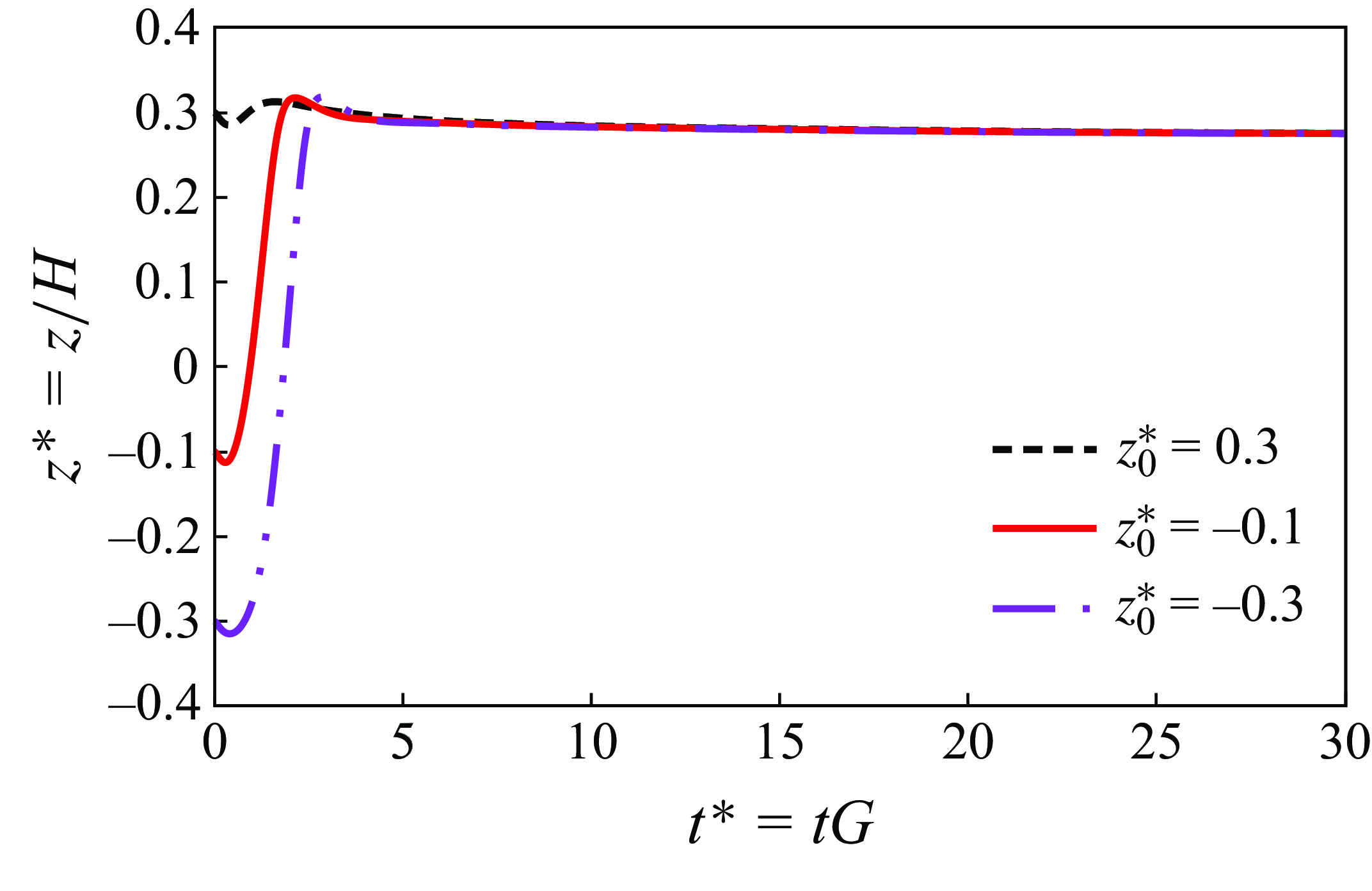
Figure 6. Effect of initial position on the final equilibrium position of a hot prolate particle at ${Gr}=60$
and
${Gr}=60$
and $\textit{Re}_p=1$
.
$\textit{Re}_p=1$
.

Figure 7. Effect of initial position on the final equilibrium position of a hot prolate particle at ${Gr}=60$
and
${Gr}=60$
and $\textit{Re}_p=10.$
4.2.1. Effect of initial position
In this case, the particle is initially positioned on the vertical centre plane of the domain ( $xz$
), while its initial vertical position (
$xz$
), while its initial vertical position ( $z^*=z/H$
) is varied across different set-ups. The particle major radius is initially aligned along the
$z^*=z/H$
) is varied across different set-ups. The particle major radius is initially aligned along the $x$
-direction (
$x$
-direction ( $\theta = \pi /2$
,
$\theta = \pi /2$
, $\phi =0$
). To study the effect of particle initial position on its migration trajectory and equilibrium position, three initial positions of
$\phi =0$
). To study the effect of particle initial position on its migration trajectory and equilibrium position, three initial positions of $z^*=-0.3$
,
$z^*=-0.3$
, $-0.1$
,
$-0.1$
, $+0.3$
at two particle Reynolds numbers of
$+0.3$
at two particle Reynolds numbers of $\textit{Re}_p = 1$
and 10 are investigated.
$\textit{Re}_p = 1$
and 10 are investigated.
Figures 6 and 7 illustrate the particle migration trajectory and equilibrium position for different initial positions at $\textit{Re}_p = 1$
and
$\textit{Re}_p = 1$
and $10$
, respectively. It can be observed that in both cases, the initial position only affects the transient part of the particle motion, without influencing the final particle equilibrium position. Natural convection forces the system to have a single off-centre equilibrium position, breaking the pitchfork bifurcation phenomenon. In other words, the particle ultimately reaches the same position, regardless of whether it was released initially in the lower or upper half of the channel.
$10$
, respectively. It can be observed that in both cases, the initial position only affects the transient part of the particle motion, without influencing the final particle equilibrium position. Natural convection forces the system to have a single off-centre equilibrium position, breaking the pitchfork bifurcation phenomenon. In other words, the particle ultimately reaches the same position, regardless of whether it was released initially in the lower or upper half of the channel.
Although the equilibrium position of a neutrally buoyant isothermal particle at low Reynolds numbers is at the centre of the domain (see figure 3), this is not the case any more for the non-isothermal case. The particle equilibrium position shifts to $z^*=0.275$
for
$z^*=0.275$
for $\textit{Re}_p = 1$
(figure 6). For
$\textit{Re}_p = 1$
(figure 6). For $\textit{Re}_p = 10$
, the equilibrium position, which for a neutrally buoyant particle in an isothermal flow was located at
$\textit{Re}_p = 10$
, the equilibrium position, which for a neutrally buoyant particle in an isothermal flow was located at $z^*=\pm 0.14$
, now shifts to
$z^*=\pm 0.14$
, now shifts to $z^*=0.08$
in the non-isothermal case, showing the effect of heat transfer on the final location of the particle.
$z^*=0.08$
in the non-isothermal case, showing the effect of heat transfer on the final location of the particle.
4.2.2. Effect of initial orientation
To investigate the effect of the initial orientation of the hot prolate particle on its dynamic behaviour, six different initial orientations were examined by varying $\theta$
and
$\theta$
and $\phi$
. The Reynolds and Grashof numbers are kept constant and equal to
$\phi$
. The Reynolds and Grashof numbers are kept constant and equal to $\textit{Re}_p=1$
and
$\textit{Re}_p=1$
and ${Gr}=40$
, respectively. Next, we examine the influence of two initial orientations across a range of Grashof numbers, from
${Gr}=40$
, respectively. Next, we examine the influence of two initial orientations across a range of Grashof numbers, from ${Gr}=35$
to 160, while keeping the Reynolds number fixed at
${Gr}=35$
to 160, while keeping the Reynolds number fixed at $\textit{Re}_p=1$
. The migration trajectory in two initial orientations is considered: in the first case, the major axis is initially aligned in the
$\textit{Re}_p=1$
. The migration trajectory in two initial orientations is considered: in the first case, the major axis is initially aligned in the $x$
direction (
$x$
direction ( $\theta =\pi /2, \phi =0$
); in the second one, the major axis is aligned along the
$\theta =\pi /2, \phi =0$
); in the second one, the major axis is aligned along the $y$
direction (
$y$
direction ( $\theta =\pi /2, \phi =\pi /2$
).
$\theta =\pi /2, \phi =\pi /2$
).
As shown in figure 8, all initial orientations lead to the same migration trajectory and rotation pattern, with the exception of the particle whose major axis is initially aligned with the $x$
direction (i.e.
$x$
direction (i.e. $\theta =\pi /2, \phi =0$
, black line in figure 8). In this particular case, the particle exhibits an oscillatory tumbling motion and the final equilibrium position is not stable. For particles with other initial orientations, a stable equilibrium position is eventually reached, approximately aligned with the maximum point of the oscillatory position of the particle with
$\theta =\pi /2, \phi =0$
, black line in figure 8). In this particular case, the particle exhibits an oscillatory tumbling motion and the final equilibrium position is not stable. For particles with other initial orientations, a stable equilibrium position is eventually reached, approximately aligned with the maximum point of the oscillatory position of the particle with $\theta =\pi /2, \phi =0$
. In all these cases except (
$\theta =\pi /2, \phi =0$
. In all these cases except ( $\theta =\pi /2, \phi =0$
), the major axis of the prolate particle becomes finally aligned with the
$\theta =\pi /2, \phi =0$
), the major axis of the prolate particle becomes finally aligned with the $y$
-direction and the particle experiences a pure log-rolling motion.
$y$
-direction and the particle experiences a pure log-rolling motion.
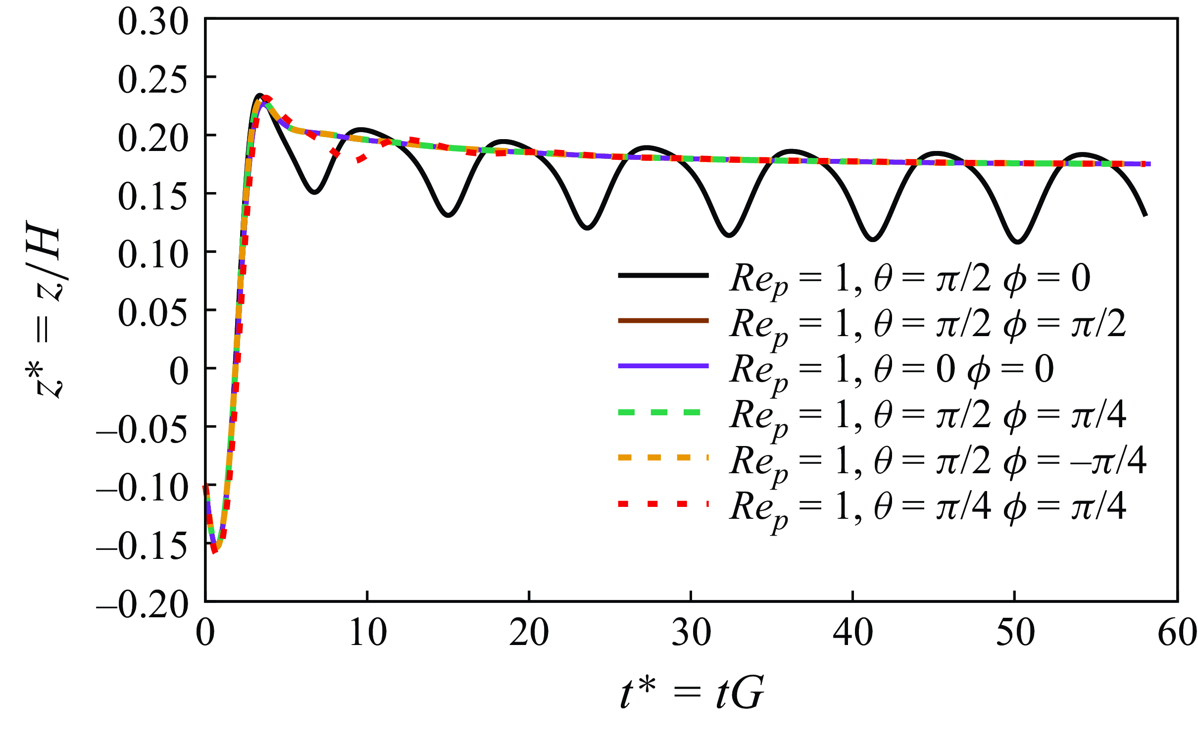
Figure 8. Effect of initial orientation on the trajectory of a hot prolate particle in a Couette flow at $\textit{Re}_p=1$
(
$\textit{Re}_p=1$
( ${Gr}=40$
in all cases).
${Gr}=40$
in all cases).
The influence of initial orientation for $35 \leqslant {Gr} \leqslant 160$
is depicted in figure 9. The results indicate that at low Grashof numbers (
$35 \leqslant {Gr} \leqslant 160$
is depicted in figure 9. The results indicate that at low Grashof numbers ( ${Gr}\leqslant 50$
), the initial orientation has a notable effect on both rotational behaviour and final state of the particle. Our simulations show that particles with their major axis initially aligned along the
${Gr}\leqslant 50$
), the initial orientation has a notable effect on both rotational behaviour and final state of the particle. Our simulations show that particles with their major axis initially aligned along the $x$
-axis exhibit a tumbling motion due to shear rate, while those aligned with the
$x$
-axis exhibit a tumbling motion due to shear rate, while those aligned with the $y$
-axis demonstrate a log-rolling motion. In the
$y$
-axis demonstrate a log-rolling motion. In the $y$
-axis-aligned case, the initial oscillatory behaviour gradually diminishes, and the particle stabilises at a distance roughly matching the peak of the oscillatory equilibrium position of the
$y$
-axis-aligned case, the initial oscillatory behaviour gradually diminishes, and the particle stabilises at a distance roughly matching the peak of the oscillatory equilibrium position of the $x$
-axis-aligned particle during its tumbling motion. At higher Grashof numbers (
$x$
-axis-aligned particle during its tumbling motion. At higher Grashof numbers ( ${Gr}\geqslant 60$
), the initial orientation of the particle has a negligible impact on both rotational behaviour and final equilibrium position. For these high Grashof numbers, the particle motion converges to a log-rolling state at a constant transverse (
${Gr}\geqslant 60$
), the initial orientation of the particle has a negligible impact on both rotational behaviour and final equilibrium position. For these high Grashof numbers, the particle motion converges to a log-rolling state at a constant transverse ( $z$
) position. It is seen that in contrast to the isothermal case (§ 4.1), we now have log-rolling motion as well for the cases with initial orientation of (
$z$
) position. It is seen that in contrast to the isothermal case (§ 4.1), we now have log-rolling motion as well for the cases with initial orientation of ( $\theta =\pi /2, \phi =0$
). Still, as the Grashof number increases, the particle shifts further upwards and the effect of orientation becomes less evident.
$\theta =\pi /2, \phi =0$
). Still, as the Grashof number increases, the particle shifts further upwards and the effect of orientation becomes less evident.
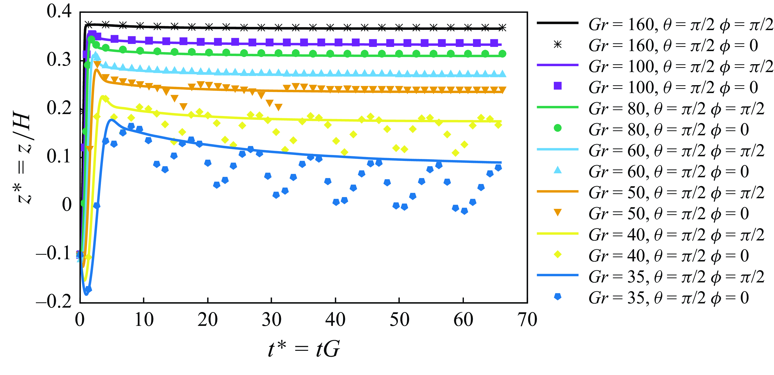
Figure 9. Effect of initial orientation on the trajectory of a hot prolate particle in a Couette flow at different Grashof numbers ( $\textit{Re}_p=1$
in all cases).
$\textit{Re}_p=1$
in all cases).
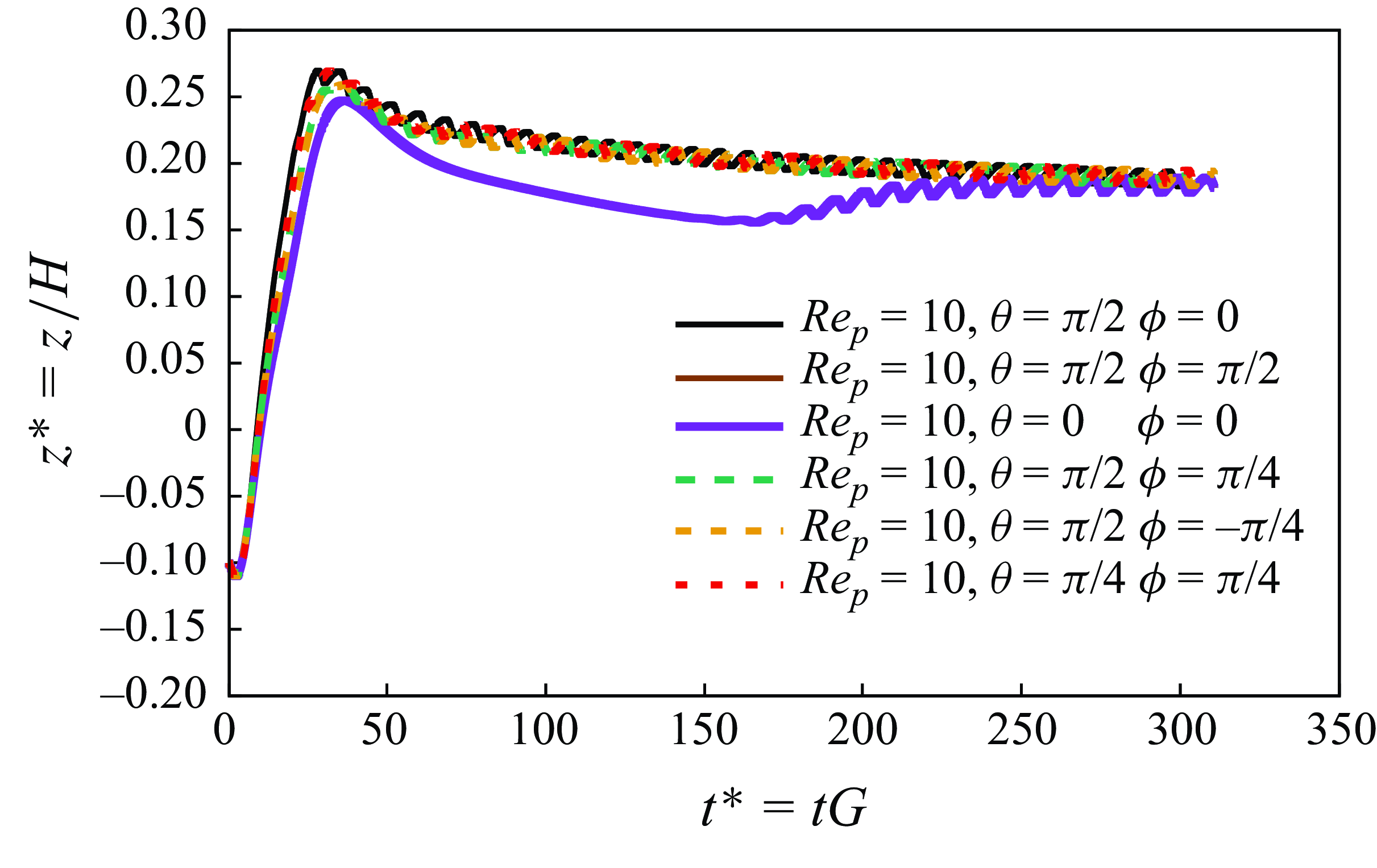
Figure 10. Effect of initial orientation on the rotation of a hot prolate particle in a Couette flow at $\textit{Re}_p=10$
(
$\textit{Re}_p=10$
( ${Gr}=80$
in all cases).
${Gr}=80$
in all cases).
Figure 10 illustrates the effect of initial orientation at $\textit{Re}_p = 10$
, which is slightly above the first critical Reynolds threshold for a neutrally buoyant isothermal particle, as shown earlier in § 4.1. In this case, the orientation of the hot particle initially creates two distinct behaviours. However, as time progresses, the particle’s dynamics becomes independent of its starting orientation. When the particle is initially aligned perpendicular to the flow direction (i.e., for
$\textit{Re}_p = 10$
, which is slightly above the first critical Reynolds threshold for a neutrally buoyant isothermal particle, as shown earlier in § 4.1. In this case, the orientation of the hot particle initially creates two distinct behaviours. However, as time progresses, the particle’s dynamics becomes independent of its starting orientation. When the particle is initially aligned perpendicular to the flow direction (i.e., for $\theta = \pi /2$
,
$\theta = \pi /2$
, $\phi =\pi /2$
or
$\phi =\pi /2$
or $\theta = 0$
,
$\theta = 0$
, $\phi =0$
), it first moves upward (like for all other cases) before migrating downward with a log-rolling rotation. Eventually, after dimensionless time
$\phi =0$
), it first moves upward (like for all other cases) before migrating downward with a log-rolling rotation. Eventually, after dimensionless time $t^* = 180$
, the rotational mechanism transitions from log-rolling to tumbling, and the particle migrates to its final equilibrium position, which remains the same among different initial orientations. The final equilibrium position is
$t^* = 180$
, the rotational mechanism transitions from log-rolling to tumbling, and the particle migrates to its final equilibrium position, which remains the same among different initial orientations. The final equilibrium position is $z^*\approx 0.19$
for all cases. By comparing figure 10 (
$z^*\approx 0.19$
for all cases. By comparing figure 10 ( $\textit{Re}_p=10$
) with figure 8 (
$\textit{Re}_p=10$
) with figure 8 ( $\textit{Re}_p=1$
), we can conclude that by increasing the Reynolds number, particle inertia dominates over the initial orientation, bringing all particles to the same final location with reduced oscillatory motion.
$\textit{Re}_p=1$
), we can conclude that by increasing the Reynolds number, particle inertia dominates over the initial orientation, bringing all particles to the same final location with reduced oscillatory motion.
Figure 11 shows the effect of initial orientation at $\textit{Re}_p = 30$
. At this Reynolds number, the initial orientation of the hot particle has minimal impact on its final equilibrium position and its final rotational mode. The combined results of figures 8–11 indicate that as the Reynolds number increases, the particle’s behaviour becomes independent of its initial orientation. Both the final equilibrium position and the rotation mode will be the same regardless of the initial orientations.
$\textit{Re}_p = 30$
. At this Reynolds number, the initial orientation of the hot particle has minimal impact on its final equilibrium position and its final rotational mode. The combined results of figures 8–11 indicate that as the Reynolds number increases, the particle’s behaviour becomes independent of its initial orientation. Both the final equilibrium position and the rotation mode will be the same regardless of the initial orientations.
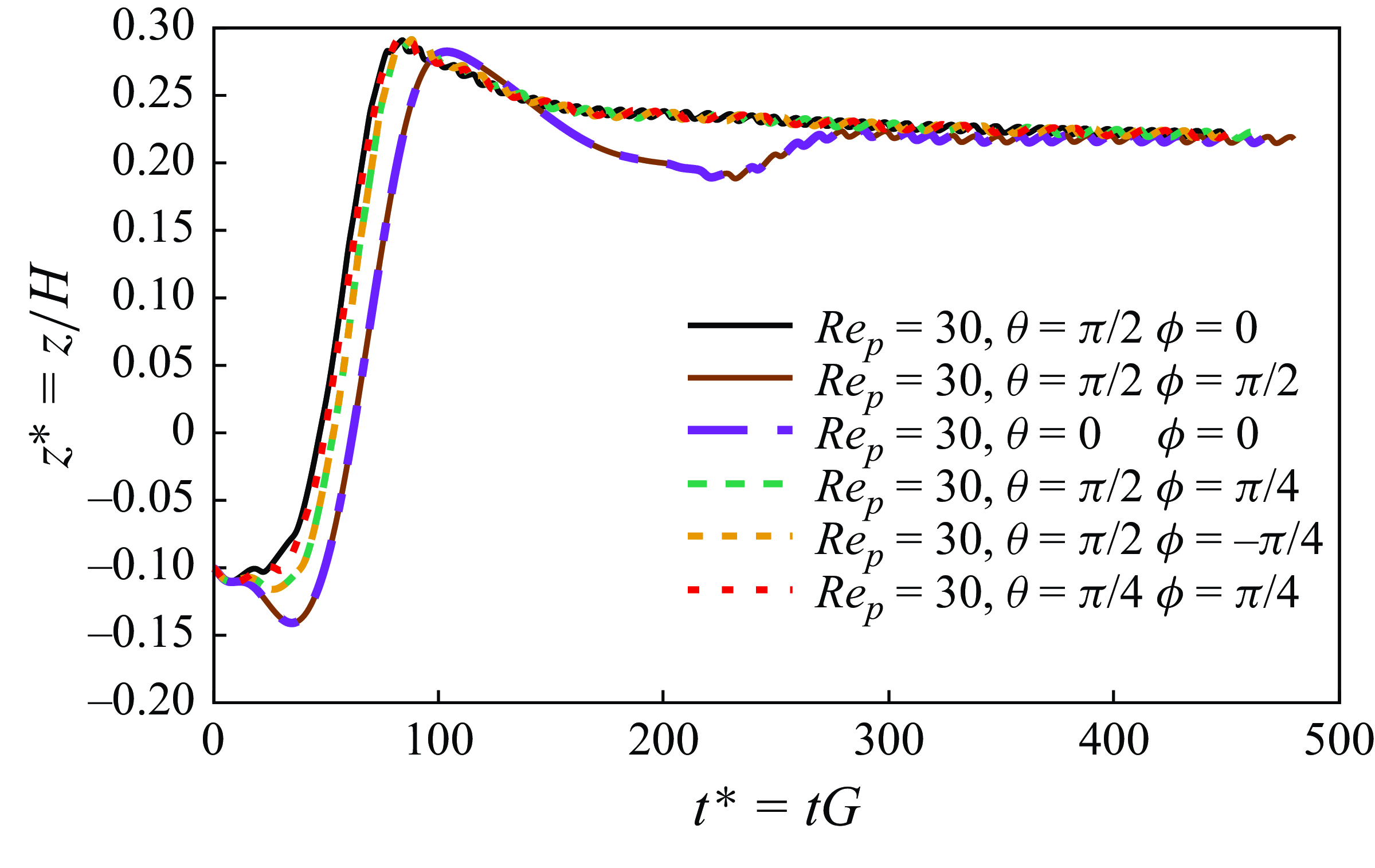
Figure 11. Effect of initial orientation on the rotation of a hot prolate particle in a Couette flow at $\textit{Re}_p=30$
(
$\textit{Re}_p=30$
( ${Gr}=80$
in all cases).
${Gr}=80$
in all cases).
4.2.3. Effect of Grashof number
In this section, the effect of Grashof number on the hot prolate particle in shear flow is investigated. The Grashof number, which characterises the relative influence of buoyancy compared with viscous forces, is varied to observe its impact on the natural convection around the particle. The analysis is conducted at three distinct Reynolds numbers: $\textit{Re}_p=1,10$
and
$\textit{Re}_p=1,10$
and $30$
.
$30$
.
At $\textit{Re}_p=1$
, hydrodynamic forces keep a neutrally buoyant particle in the centreline of the domain. However, the introduction of gravitational force, along with the convection-induced force, alters the balance of forces acting on the particle. The transverse trajectory of the particle for various Grashof numbers at
$\textit{Re}_p=1$
, hydrodynamic forces keep a neutrally buoyant particle in the centreline of the domain. However, the introduction of gravitational force, along with the convection-induced force, alters the balance of forces acting on the particle. The transverse trajectory of the particle for various Grashof numbers at $\textit{Re}_p=1$
(figure 12) confirms that when the Grashof number is 33 or lower, the gravitational force dominates, causing the particle to sediment and collide with the lower wall. This indicates that the buoyancy induced by natural convection is insufficient to counteract gravitation. As the Grashof number becomes larger, for
$\textit{Re}_p=1$
(figure 12) confirms that when the Grashof number is 33 or lower, the gravitational force dominates, causing the particle to sediment and collide with the lower wall. This indicates that the buoyancy induced by natural convection is insufficient to counteract gravitation. As the Grashof number becomes larger, for $35\leqslant {Gr} \lt 50$
, the buoyancy-driven drag from natural convection, along with the shear-gradient lift force, surpasses the gravitational force, driving the particle upwards. However, once the particle crosses above the centreline, the direction of the shear-gradient lift force reverses, acting in the same direction as gravity (downwards). This reversal leads to a balance of forces, stabilising the particle at some position above the centreline, where all these forces counteract each other. By increasing further the Grashof number up to
$35\leqslant {Gr} \lt 50$
, the buoyancy-driven drag from natural convection, along with the shear-gradient lift force, surpasses the gravitational force, driving the particle upwards. However, once the particle crosses above the centreline, the direction of the shear-gradient lift force reverses, acting in the same direction as gravity (downwards). This reversal leads to a balance of forces, stabilising the particle at some position above the centreline, where all these forces counteract each other. By increasing further the Grashof number up to ${Gr} = 200$
, the overall migration behaviour of the particle does not change qualitatively. However, the increased buoyancy causes the final equilibrium position of the particle to shift closer to the upper wall for higher Grashof values.
${Gr} = 200$
, the overall migration behaviour of the particle does not change qualitatively. However, the increased buoyancy causes the final equilibrium position of the particle to shift closer to the upper wall for higher Grashof values.
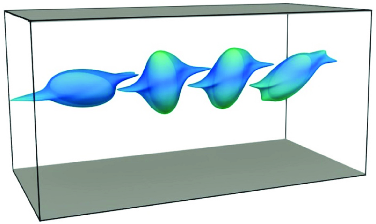
Snapshots of the particle orientation and iso-surfaces of the $Q$
-criterion, coloured by normalised temperature, are shown in figure 13. These snapshots capture two arbitrary time instances after the particle reaches its final equilibrium position for
$Q$
-criterion, coloured by normalised temperature, are shown in figure 13. These snapshots capture two arbitrary time instances after the particle reaches its final equilibrium position for ${Gr} = 200$
, 50 and 40. In all cases, the Reynolds number is
${Gr} = 200$
, 50 and 40. In all cases, the Reynolds number is $\textit{Re}_p = 1$
. The behaviour of the particle is quite different when the Grashof number is changed. For
$\textit{Re}_p = 1$
. The behaviour of the particle is quite different when the Grashof number is changed. For ${Gr} = 200$
, the particle finally takes an equilibrium position close to the upper wall with its major axis aligned with the
${Gr} = 200$
, the particle finally takes an equilibrium position close to the upper wall with its major axis aligned with the $x$
-axis; it does not experience further rotation. Conversely, for
$x$
-axis; it does not experience further rotation. Conversely, for ${Gr} = 50$
, the particle experiences a log-rolling rotation and is aligned along the
${Gr} = 50$
, the particle experiences a log-rolling rotation and is aligned along the $y$
-axis around an equilibrium position lower than for
$y$
-axis around an equilibrium position lower than for ${Gr} = 200$
. Finally, for
${Gr} = 200$
. Finally, for ${Gr} = 40$
, due to the change in the force, the particle oscillates between two transverse (
${Gr} = 40$
, due to the change in the force, the particle oscillates between two transverse ( $z$
) locations, and its rotation is tumbling.
$z$
) locations, and its rotation is tumbling.

Figure 12. Effect of Grashof numbers on the migration trajectory of a hot prolate particle in a Couette flow ( $\textit{Re}_p=1$
in all cases).
$\textit{Re}_p=1$
in all cases).
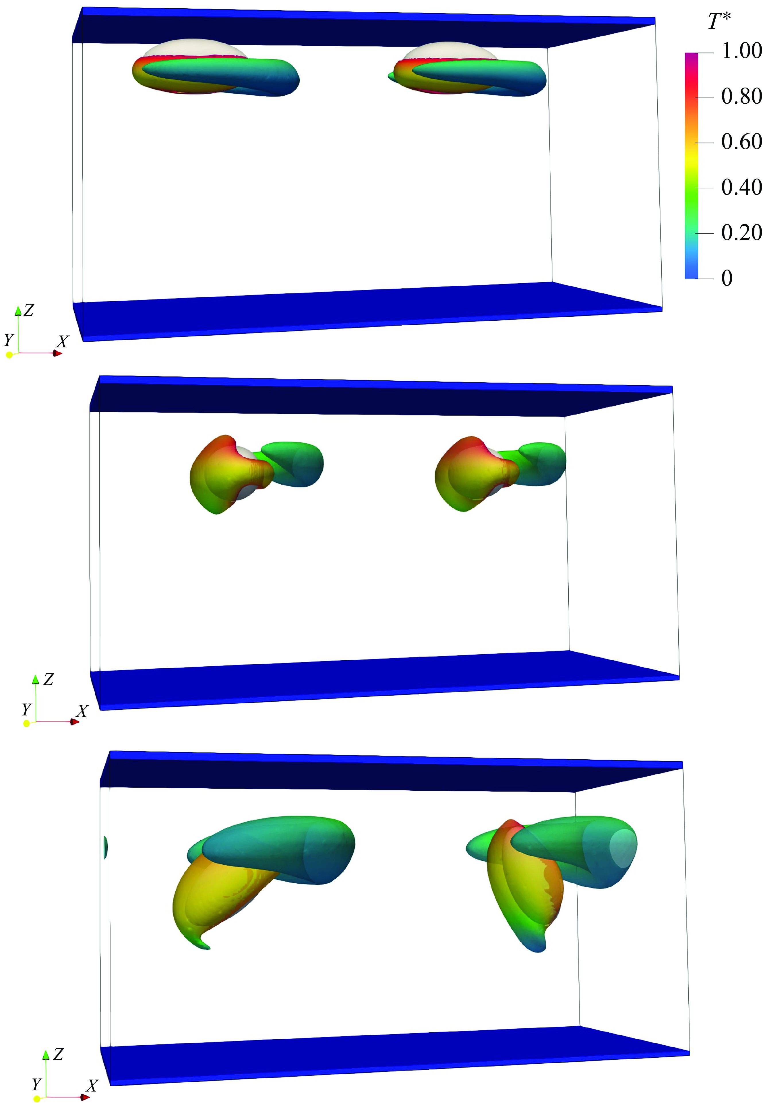
Figure 13. Particle orientation and iso-surface of the $Q$
-criterion for
$Q$
-criterion for $10\,\%$
of peak value coloured by normalised temperature for a case with
$10\,\%$
of peak value coloured by normalised temperature for a case with ${Gr}=200$
,
${Gr}=200$
, ${Gr}=50$
and
${Gr}=50$
and ${Gr}=40$
from top to bottom, respectively (
${Gr}=40$
from top to bottom, respectively ( $\textit{Re}_p=1$
in all cases).
$\textit{Re}_p=1$
in all cases).
Figure 14 illustrates the migration trajectory of the hot prolate particle at different Grashof numbers for $\textit{Re}_p = 10$
. For the neutrally buoyant particle at
$\textit{Re}_p = 10$
. For the neutrally buoyant particle at $\textit{Re}_p = 10$
, we already observed that the particle reaches an off-centre equilibrium position near the centreline (see figure 3). However, in the presence of gravity and heat transfer, the bifurcation of the equilibrium position disappears (see figure 7). Based on these results, the hot prolate particle moves into a single equilibrium state, either on the upper half of the channel or near the bottom wall, depending on the Grashof number. According to figure 14, at lower Grashof numbers (
$\textit{Re}_p = 10$
, we already observed that the particle reaches an off-centre equilibrium position near the centreline (see figure 3). However, in the presence of gravity and heat transfer, the bifurcation of the equilibrium position disappears (see figure 7). Based on these results, the hot prolate particle moves into a single equilibrium state, either on the upper half of the channel or near the bottom wall, depending on the Grashof number. According to figure 14, at lower Grashof numbers ( ${Gr}\leqslant 50$
), gravitational forces dominate, drawing the particle towards the bottom wall, where it rotates close to the surface. The presence of the wall alters the hydrodynamic forces, leading to larger oscillations. At moderate Grashof numbers, the particle settles into an equilibrium position above the centreline and the oscillation becomes less pronounced. At the highest examined Grashof number of
${Gr}\leqslant 50$
), gravitational forces dominate, drawing the particle towards the bottom wall, where it rotates close to the surface. The presence of the wall alters the hydrodynamic forces, leading to larger oscillations. At moderate Grashof numbers, the particle settles into an equilibrium position above the centreline and the oscillation becomes less pronounced. At the highest examined Grashof number of ${Gr}= 160$
, the amplitude of the oscillations increases again. As already observed with
${Gr}= 160$
, the amplitude of the oscillations increases again. As already observed with $\textit{Re}_p=1$
, increasing the Grashof number at
$\textit{Re}_p=1$
, increasing the Grashof number at $\textit{Re}_p=10$
shifts the particle’s equilibrium position towards the upper half of the domain, where it remains at a certain distance from the top wall. Throughout the range of Grashof numbers studied, the particle consistently exhibits a tumbling rotation.
$\textit{Re}_p=10$
shifts the particle’s equilibrium position towards the upper half of the domain, where it remains at a certain distance from the top wall. Throughout the range of Grashof numbers studied, the particle consistently exhibits a tumbling rotation.
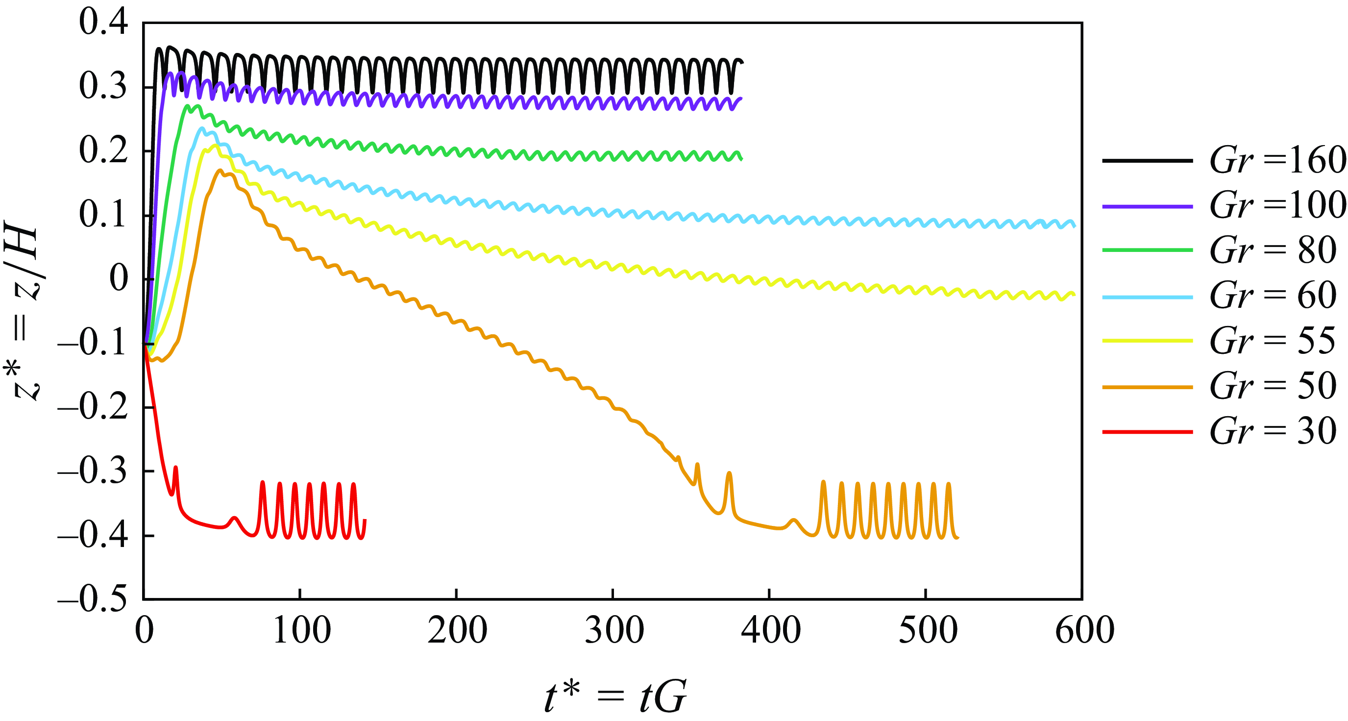
Figure 14. Effect of Grashof numbers on the migration trajectory of a hot prolate particle in a Couette flow ( $\textit{Re}_p=10$
in all cases).
$\textit{Re}_p=10$
in all cases).
Finally, the effect of the Grashof number for the case with $\textit{Re}_p=30$
is shown in figure 15. This Reynolds number is larger than the first critical Reynolds number for a neutrally buoyant isothermal particle. Despite this, no bifurcation of the equilibrium position is observed for the hot prolate particle. Instead, the particle exhibits two distinct equilibrium behaviours: one close to the bottom wall (
$\textit{Re}_p=30$
is shown in figure 15. This Reynolds number is larger than the first critical Reynolds number for a neutrally buoyant isothermal particle. Despite this, no bifurcation of the equilibrium position is observed for the hot prolate particle. Instead, the particle exhibits two distinct equilibrium behaviours: one close to the bottom wall ( ${Gr \leqslant 40}$
), and another one in the top half of the domain for moderate and high Grashof numbers (
${Gr \leqslant 40}$
), and another one in the top half of the domain for moderate and high Grashof numbers ( ${Gr \geqslant 50}$
). As observed, the equilibrium positions at this
${Gr \geqslant 50}$
). As observed, the equilibrium positions at this $\textit{Re}_p=30$
for
$\textit{Re}_p=30$
for ${Gr=160}$
and
${Gr=160}$
and ${Gr=100}$
are lower compared with those at smaller Reynolds numbers. This trend indicates that, with increasing
${Gr=100}$
are lower compared with those at smaller Reynolds numbers. This trend indicates that, with increasing $\textit{Re}_p$
, the influence of the wall-induced lift force becomes more prominent, pushing the particle further away from the wall. As the particle migrates away from the wall, its slip velocity decreases, leading to a reduction in the Saffman lift force. Consequently, the particle reaches equilibrium at a lower vertical position within the domain.
$\textit{Re}_p$
, the influence of the wall-induced lift force becomes more prominent, pushing the particle further away from the wall. As the particle migrates away from the wall, its slip velocity decreases, leading to a reduction in the Saffman lift force. Consequently, the particle reaches equilibrium at a lower vertical position within the domain.
For all considered Grashof numbers with $\textit{Re}_p=30$
, the prolate particle demonstrates a tumbling rotational motion, similar to the behaviour seen at
$\textit{Re}_p=30$
, the prolate particle demonstrates a tumbling rotational motion, similar to the behaviour seen at $\textit{Re}_p=10$
, though the amplitude of the oscillations is significantly reduced at
$\textit{Re}_p=10$
, though the amplitude of the oscillations is significantly reduced at $\textit{Re}_p=30$
.
$\textit{Re}_p=30$
.
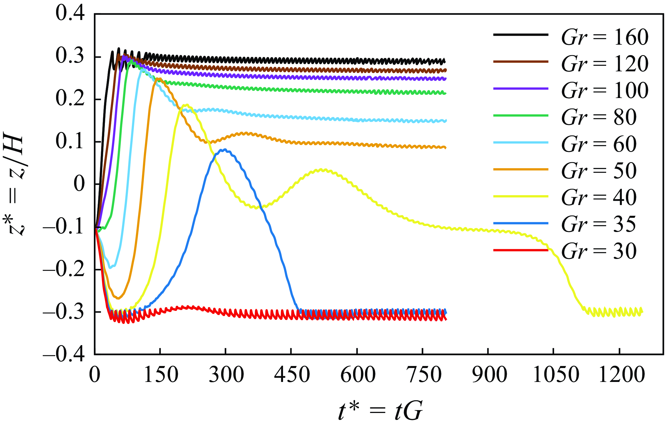
Figure 15. Effect of Grashof numbers on the migration trajectory of a hot prolate particle in a Couette flow ( $\textit{Re}_p=30$
in all cases).
$\textit{Re}_p=30$
in all cases).
4.2.4. Effect of Reynolds number
In § 4.1, we observed that for an isothermal shear flow, a prolate particle exhibits three distinct behaviours depending on the particle Reynolds number. Below the first critical Reynolds number, the particle reaches a single equilibrium position at the centre of the shear flow. Beyond this critical value, a pitchfork bifurcation occurs, leading to two symmetric equilibrium positions. As $\textit{Re}_p$
reaches the second critical Reynolds number, the equilibrium position shifts back towards the centre of the domain. Now, in this section, we aim to explore how the behaviour of a heated particle differs from that of an isothermal particle, focusing on how variations in the particle Reynolds number,
$\textit{Re}_p$
reaches the second critical Reynolds number, the equilibrium position shifts back towards the centre of the domain. Now, in this section, we aim to explore how the behaviour of a heated particle differs from that of an isothermal particle, focusing on how variations in the particle Reynolds number, $\textit{Re}_p$
, affect both the equilibrium position and the particle motion.
$\textit{Re}_p$
, affect both the equilibrium position and the particle motion.
We consider the case of a hot prolate particle with a Grashof number of ${Gr}=80$
across a range of Reynolds numbers from
${Gr}=80$
across a range of Reynolds numbers from $\textit{Re}_p=1$
to 90. As illustrated in figures 16 and 17, for
$\textit{Re}_p=1$
to 90. As illustrated in figures 16 and 17, for $\textit{Re}_p=1$
, the particle migrates towards the upper side of the domain, stabilising at
$\textit{Re}_p=1$
, the particle migrates towards the upper side of the domain, stabilising at $z^*=0.31$
. This location is different from the isothermal particle that stabilises at
$z^*=0.31$
. This location is different from the isothermal particle that stabilises at $z^*=0$
for similar Reynolds numbers (figure 3). By further increasing the Reynolds number to
$z^*=0$
for similar Reynolds numbers (figure 3). By further increasing the Reynolds number to $\textit{Re}_p=10$
, the equilibrium position shifts downwards to
$\textit{Re}_p=10$
, the equilibrium position shifts downwards to $z^*=0.19$
. As the Reynolds number increases further, the equilibrium position gradually moves upwards, eventually stabilising at approximately
$z^*=0.19$
. As the Reynolds number increases further, the equilibrium position gradually moves upwards, eventually stabilising at approximately $z^*\approx 0.26$
for Reynolds numbers between 50 and 70. At
$z^*\approx 0.26$
for Reynolds numbers between 50 and 70. At $\textit{Re}_p=70$
, the particle initially exhibits chaotic motion. However, after some time, it unexpectedly settles into an off-centre equilibrium position on the upper side. To investigate whether this behaviour is influenced by the particle’s initial orientation, a simulation was conducted with the prolate particle aligned in the
$\textit{Re}_p=70$
, the particle initially exhibits chaotic motion. However, after some time, it unexpectedly settles into an off-centre equilibrium position on the upper side. To investigate whether this behaviour is influenced by the particle’s initial orientation, a simulation was conducted with the prolate particle aligned in the $y$
-direction. This revealed that while the initial orientation affects the early chaotic motion, it does not influence the final equilibrium position. For the cases with
$y$
-direction. This revealed that while the initial orientation affects the early chaotic motion, it does not influence the final equilibrium position. For the cases with $\textit{Re}_p=75, 80$
and
$\textit{Re}_p=75, 80$
and $85$
, the chaotic motion continues throughout the duration of the simulation. Hence, these cases were not included in figure 16 to maintain clarity and facilitate a more straightforward interpretation of trends. For
$85$
, the chaotic motion continues throughout the duration of the simulation. Hence, these cases were not included in figure 16 to maintain clarity and facilitate a more straightforward interpretation of trends. For $\textit{Re}_p=90$
, after the initial chaotic behaviour, the particle eventually migrates back towards the centreline. Therefore, for the hot particle, we identified two critical Reynolds numbers as well. Below the first one, the particle’s equilibrium position shifts downwards with increasing
$\textit{Re}_p=90$
, after the initial chaotic behaviour, the particle eventually migrates back towards the centreline. Therefore, for the hot particle, we identified two critical Reynolds numbers as well. Below the first one, the particle’s equilibrium position shifts downwards with increasing $\textit{Re}_p$
; beyond this point, the trend reverses. At the second critical Reynolds number, the particle migrates to the centre region. It is important to note that no pitchfork bifurcation occurs in either case. Interestingly, beyond the first critical
$\textit{Re}_p$
; beyond this point, the trend reverses. At the second critical Reynolds number, the particle migrates to the centre region. It is important to note that no pitchfork bifurcation occurs in either case. Interestingly, beyond the first critical $\textit{Re}_p$
, the equilibrium position of the hot particle is closer to the centreline compared with that of a neutrally buoyant isothermal particle. Furthermore, the second critical Reynolds number for the hot particle is lower than that observed for the isothermal case. This suggests that thermal effects, including buoyancy-induced flow modifications and temperature-dependent forces, play a significant role in altering the particle’s migration behaviour and thresholds. However, this observation is somewhat unexpected, as the presence of the convection-induced lift force was anticipated to drive the hot particle towards a higher equilibrium position. Instead, the particle stabilises closer to the centreline, indicating a more complex interplay between thermal buoyancy, shear and inertial lift forces, and wall-induced forces than initially presumed.
$\textit{Re}_p$
, the equilibrium position of the hot particle is closer to the centreline compared with that of a neutrally buoyant isothermal particle. Furthermore, the second critical Reynolds number for the hot particle is lower than that observed for the isothermal case. This suggests that thermal effects, including buoyancy-induced flow modifications and temperature-dependent forces, play a significant role in altering the particle’s migration behaviour and thresholds. However, this observation is somewhat unexpected, as the presence of the convection-induced lift force was anticipated to drive the hot particle towards a higher equilibrium position. Instead, the particle stabilises closer to the centreline, indicating a more complex interplay between thermal buoyancy, shear and inertial lift forces, and wall-induced forces than initially presumed.
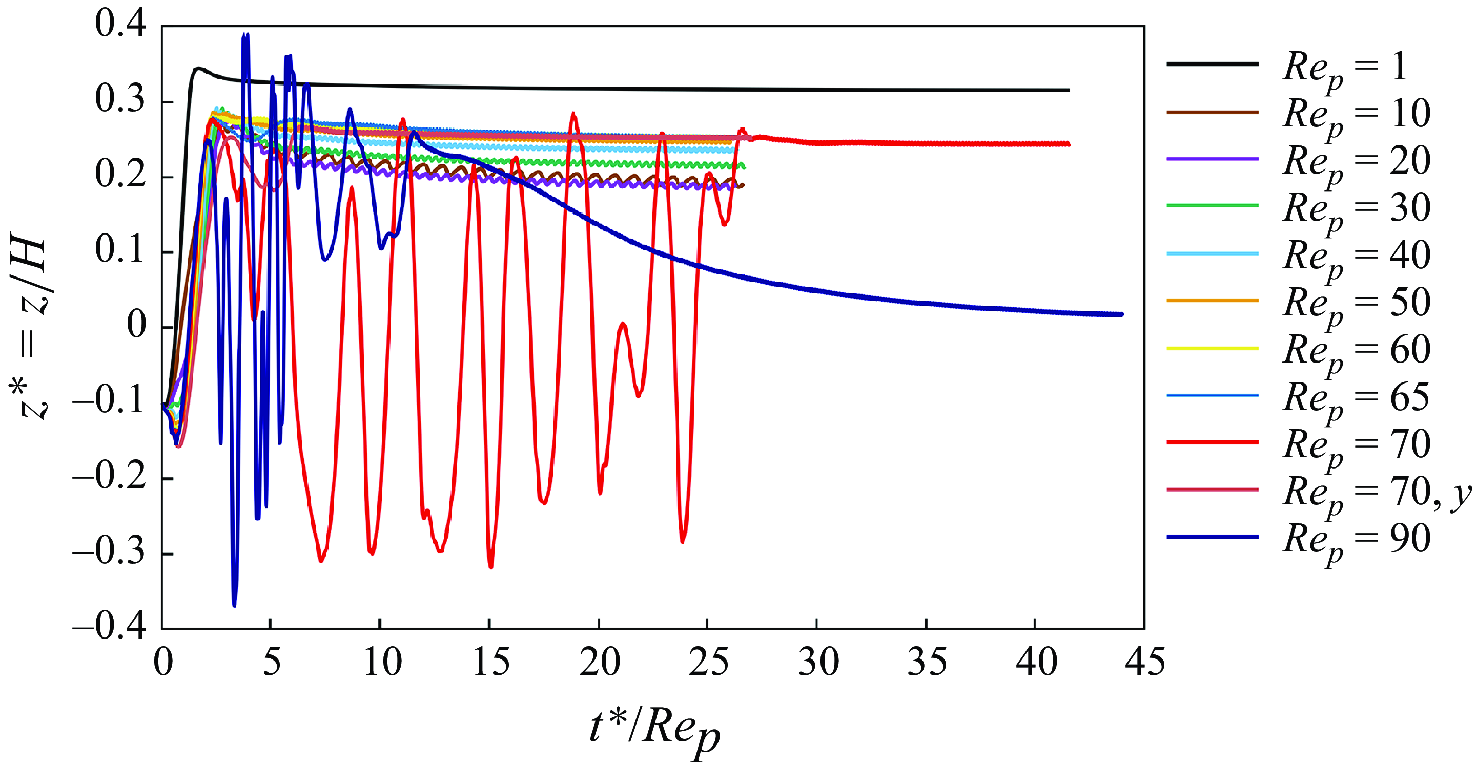
Figure 16. Effect of Reynolds number on the migration trajectory of a hot prolate particle in a Couette flow ( ${Gr}=80$
in all cases).
${Gr}=80$
in all cases).
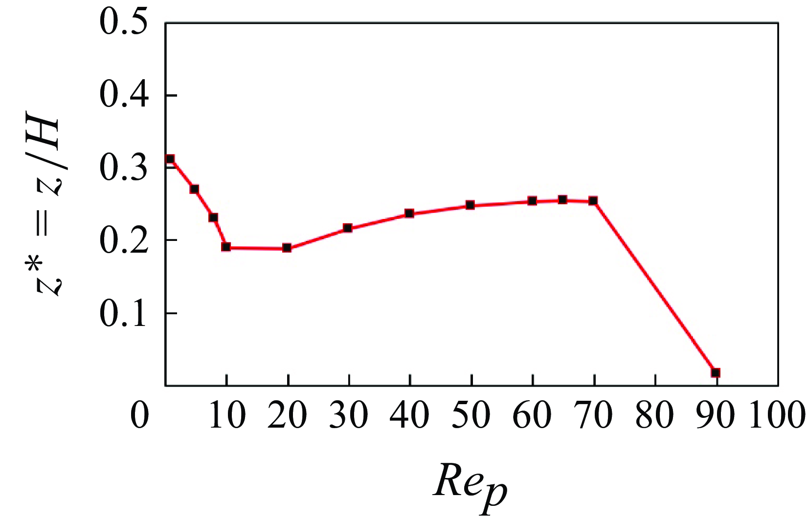
Figure 17. Final equilibrium position of a hot prolate particle as a function of particle Reynolds number in a Couette flow ( ${Gr}=80$
in all cases).
${Gr}=80$
in all cases).
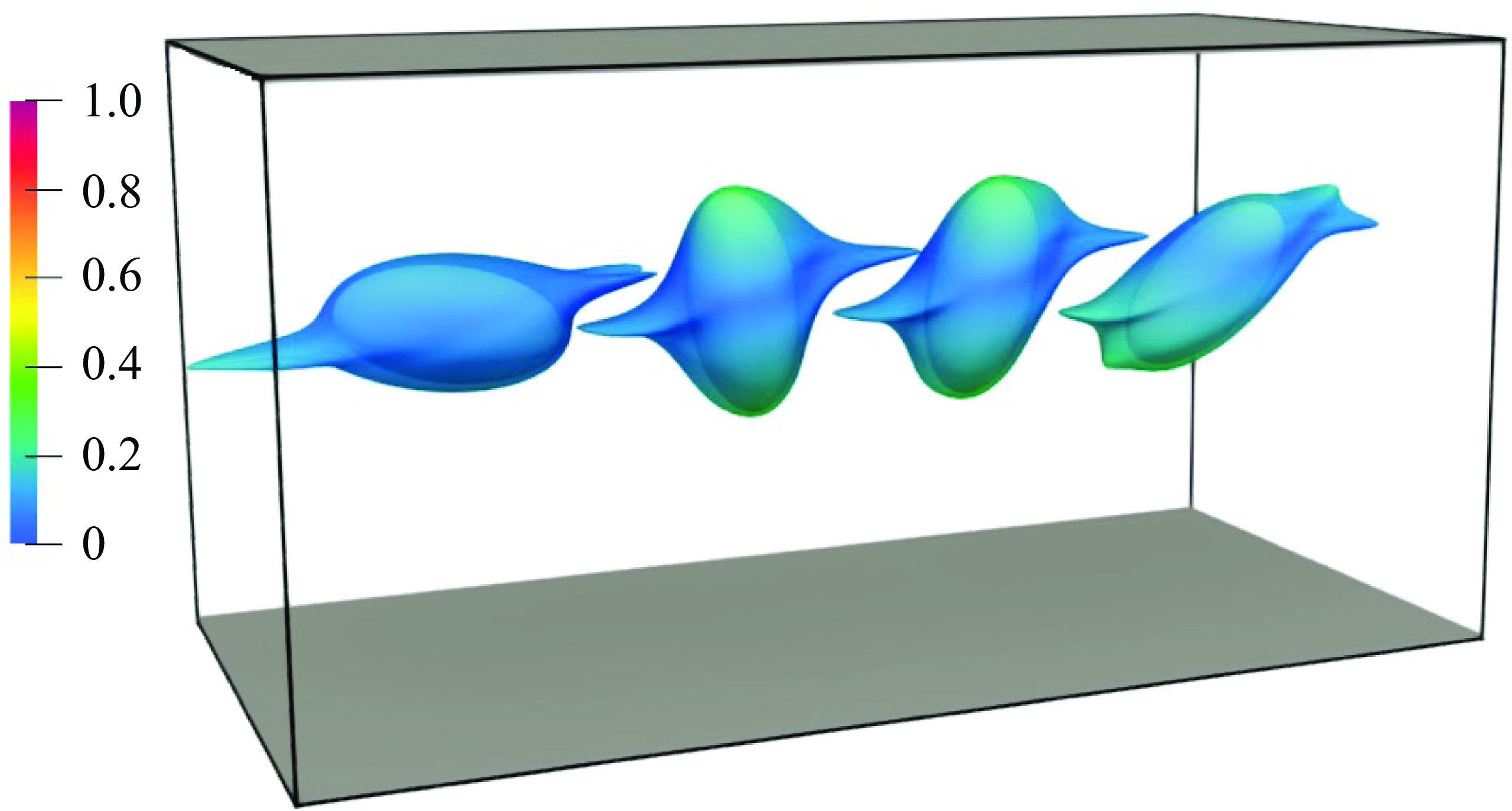
Figure 18. Iso-surface of temperature ( $T^* = 0.65$
) surrounding the particle in various orientations, after attaining the equilibrium position, coloured by
$T^* = 0.65$
) surrounding the particle in various orientations, after attaining the equilibrium position, coloured by $u^* = u/u_{{max}}$
, at
$u^* = u/u_{{max}}$
, at $\textit{Re}_p = 90$
and
$\textit{Re}_p = 90$
and ${Gr} = 80$
.
${Gr} = 80$
.
Figure 17 exhibits the variation of final transverse position versus Reynolds number. Overall, it is evident that for Reynolds numbers far below the first critical point, convective forces dominate, causing the particle to stabilise farther from the centreline towards the top side. As the Reynolds number increases, other hydrodynamic forces begin to influence the particle behaviour, resulting in a noticeable shift in the equilibrium position towards the centre. For Reynolds numbers exceeding the first critical value ( $\textit{Re}_p\approx 10$
), a slight upwards shift in the equilibrium position is observed with increasing
$\textit{Re}_p\approx 10$
), a slight upwards shift in the equilibrium position is observed with increasing $\textit{Re}_p$
. Within the range of
$\textit{Re}_p$
. Within the range of $\textit{Re}_p=50$
–70, the equilibrium position becomes relatively insensitive to changes in Reynolds number. However, at higher Reynolds numbers, the particle undergoes a period of chaotic motion before settling into equilibrium. Notably, in this range of
$\textit{Re}_p=50$
–70, the equilibrium position becomes relatively insensitive to changes in Reynolds number. However, at higher Reynolds numbers, the particle undergoes a period of chaotic motion before settling into equilibrium. Notably, in this range of $\textit{Re}_p$
, contrary to the behaviour observed in isothermal flows, no bifurcation of the equilibrium position occurs. Interestingly, at
$\textit{Re}_p$
, contrary to the behaviour observed in isothermal flows, no bifurcation of the equilibrium position occurs. Interestingly, at $\textit{Re}_p=90$
, the equilibrium position of the hot prolate particle shifts back towards the centre of the domain (
$\textit{Re}_p=90$
, the equilibrium position of the hot prolate particle shifts back towards the centre of the domain ( $z^*\approx 0$
), similar to the behaviour seen in isothermal flow conditions.
$z^*\approx 0$
), similar to the behaviour seen in isothermal flow conditions.
For $\textit{Re}_p=1$
, the motion is log-rolling, while at higher
$\textit{Re}_p=1$
, the motion is log-rolling, while at higher $\textit{Re}_p$
values, the motion becomes tumbling. Figure 18 shows the iso-surface of temperature around the particle in different orientations during the rotational period at
$\textit{Re}_p$
values, the motion becomes tumbling. Figure 18 shows the iso-surface of temperature around the particle in different orientations during the rotational period at $\textit{Re}_p=90$
and
$\textit{Re}_p=90$
and ${Gr}=80$
, after reaching the equilibrium position. Additionally, for a visualisation of the equilibrium position and particle behaviour in the final equilibrium position, the reader is referred to the accompanying video provided as Supplementary material for
${Gr}=80$
, after reaching the equilibrium position. Additionally, for a visualisation of the equilibrium position and particle behaviour in the final equilibrium position, the reader is referred to the accompanying video provided as Supplementary material for $\textit{Re}_p=60$
and
$\textit{Re}_p=60$
and $\textit{Re}_p=90$
at
$\textit{Re}_p=90$
at ${Gr}=80$
.
${Gr}=80$
.
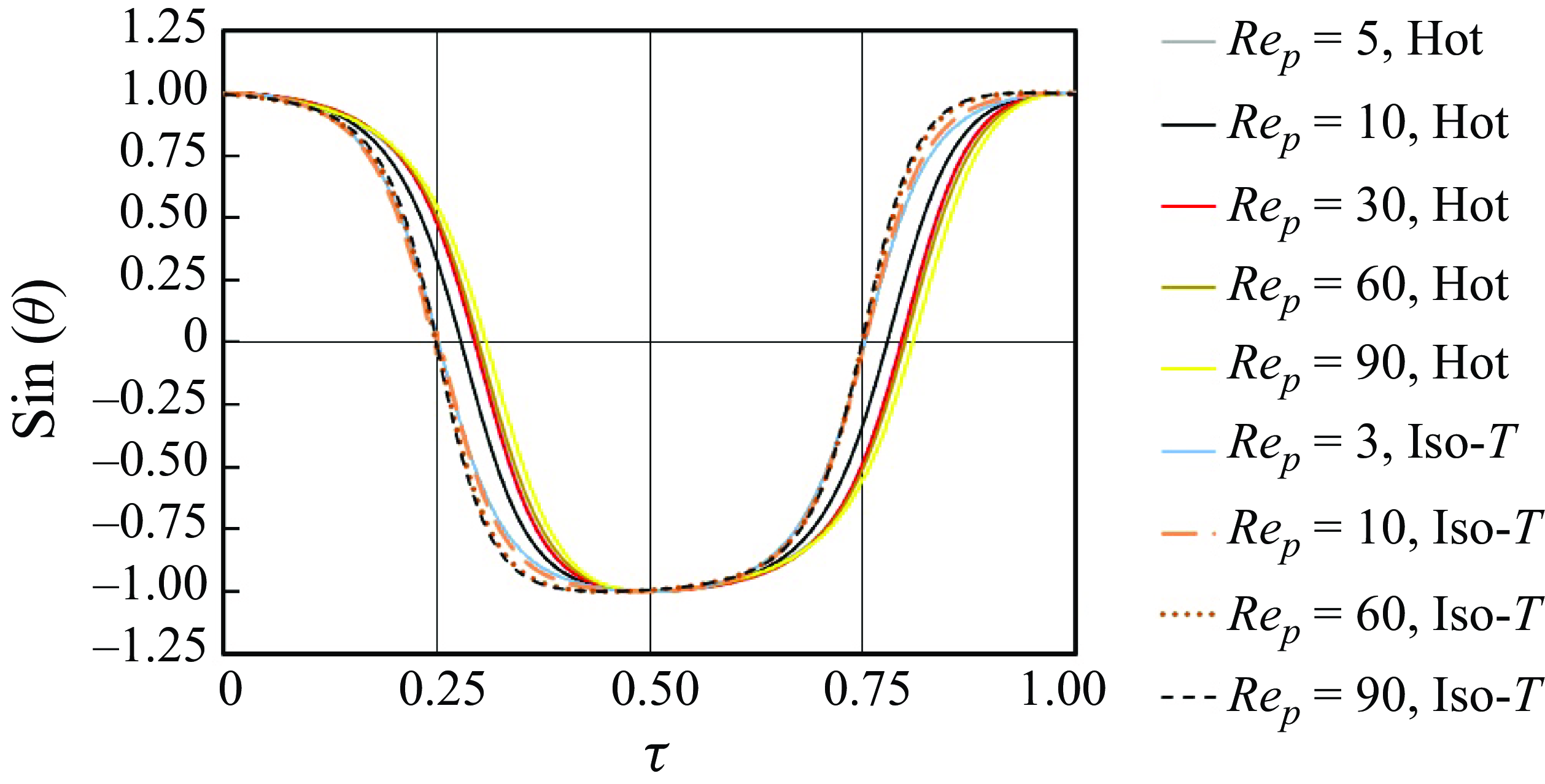
Figure 19. Orientation angle of a hot prolate particle ( ${Gr}=80$
, solid lines) and an isothermal particle (dashed lines) during the normalised rotational period.
${Gr}=80$
, solid lines) and an isothermal particle (dashed lines) during the normalised rotational period.
To further analyse the rotational behaviour of the hot prolate particle, figure 19 presents $\sin (\theta )$
over one rotational period in comparison to the neutrally buoyant isothermal particle, where
$\sin (\theta )$
over one rotational period in comparison to the neutrally buoyant isothermal particle, where $\theta$
is the angle with the
$\theta$
is the angle with the $z$
-axis. For a Grashof number of
$z$
-axis. For a Grashof number of ${Gr}=80$
, the rotation of the prolate particle is always of a tumbling nature. As depicted in this figure, the rotational behaviour shows a phase shift for the hot particle compared with the isothermal particle due to secondary flows that emerge from heat convection. The presence of a thermal gradient leads to a faster descent when the particle’s long axis is realigning with the flow, transitioning from the perpendicular orientation to the flow direction (
${Gr}=80$
, the rotation of the prolate particle is always of a tumbling nature. As depicted in this figure, the rotational behaviour shows a phase shift for the hot particle compared with the isothermal particle due to secondary flows that emerge from heat convection. The presence of a thermal gradient leads to a faster descent when the particle’s long axis is realigning with the flow, transitioning from the perpendicular orientation to the flow direction ( $\sin \theta = 0$
) to an alignment with the flow direction (
$\sin \theta = 0$
) to an alignment with the flow direction ( $\sin \theta =\pm 1$
), and a slower ascent from the flow direction to the perpendicular orientation. In the isothermal case, the rotational behaviour is more symmetric, whereas in both cases, an increase in
$\sin \theta =\pm 1$
), and a slower ascent from the flow direction to the perpendicular orientation. In the isothermal case, the rotational behaviour is more symmetric, whereas in both cases, an increase in $\textit{Re}_p$
enhances inertial effects, leading to a stronger asymmetry in rotational behaviour.
$\textit{Re}_p$
enhances inertial effects, leading to a stronger asymmetry in rotational behaviour.
At low Reynolds numbers, the rotation of a prolate particle in shear flows follows Jeffery’s theory, in which the non-dimensional period of rotation, $\tau _0$
, is a function of aspect ratio,
$\tau _0$
, is a function of aspect ratio, $r$
, and is expressed as
$r$
, and is expressed as
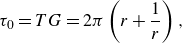 \begin{equation} \tau _0 = TG= 2\pi \left ( r+\frac { 1}{r} \right ), \end{equation}
This leads to $\tau _0 = 15.71$
for the case considered in this work. Figure 20 displays the particle’s rotational period at different
$\tau _0 = 15.71$
for the case considered in this work. Figure 20 displays the particle’s rotational period at different $\textit{Re}_p$
for a hot particle at
$\textit{Re}_p$
for a hot particle at ${Gr} = 80$
and for a neutrally buoyant isothermal particle. The results indicate that for
${Gr} = 80$
and for a neutrally buoyant isothermal particle. The results indicate that for $\textit{Re}_p \geqslant 1$
, the rotational period exceeds the prediction of Jeffery’s theory. An increase in the rotational period is observed up to
$\textit{Re}_p \geqslant 1$
, the rotational period exceeds the prediction of Jeffery’s theory. An increase in the rotational period is observed up to $\textit{Re}_p = 20$
, beyond which it remains constant until approximately
$\textit{Re}_p = 20$
, beyond which it remains constant until approximately $\textit{Re}_p = 70$
for the hot particle. This constancy, coupled with the consistent rotational behaviour shown in figure 19, suggests that the rotational motion remains unchanged for
$\textit{Re}_p = 70$
for the hot particle. This constancy, coupled with the consistent rotational behaviour shown in figure 19, suggests that the rotational motion remains unchanged for $20 \leqslant \textit{Re}_p \leqslant 70$
. For
$20 \leqslant \textit{Re}_p \leqslant 70$
. For $\textit{Re}_p = 90$
, which is beyond the second critical Reynolds number, the rotational period increases again. The hot particle, across all
$\textit{Re}_p = 90$
, which is beyond the second critical Reynolds number, the rotational period increases again. The hot particle, across all $\textit{Re}_p$
, has a shorter rotation period compared with the isothermal particle. This indicates that, in contrast to the inertia effect which increases the rotation period, the presence of the secondary flow induced by heat convection reduces it. Interestingly, in the range between the first and second critical Reynolds numbers, the effect of heat transfer suppresses the influence of flow inertia, causing the rotation period to remain constant. However, after the second critical point, the inertia effect overcomes the influence of heat transfer and the rotation period starts increasing again.
$\textit{Re}_p$
, has a shorter rotation period compared with the isothermal particle. This indicates that, in contrast to the inertia effect which increases the rotation period, the presence of the secondary flow induced by heat convection reduces it. Interestingly, in the range between the first and second critical Reynolds numbers, the effect of heat transfer suppresses the influence of flow inertia, causing the rotation period to remain constant. However, after the second critical point, the inertia effect overcomes the influence of heat transfer and the rotation period starts increasing again.

Figure 20. Non-dimensional rotational period of the hot prolate particle ( ${Gr}=80$
) and of the isothermal particle versus particle Reynolds number.
${Gr}=80$
) and of the isothermal particle versus particle Reynolds number.
Figure 21 illustrates the normalised angular velocity of the prolate particle ( $\Omega /G$
) versus
$\Omega /G$
) versus $\sin (\theta )$
during one rotational period. The overall shape of the profile remains consistent across all cases, with the minimum velocity occurring when the major axis of the prolate particle aligns with the flow (
$\sin (\theta )$
during one rotational period. The overall shape of the profile remains consistent across all cases, with the minimum velocity occurring when the major axis of the prolate particle aligns with the flow ( $x$
) direction, and the maximum velocity observed around
$x$
) direction, and the maximum velocity observed around $\theta = 14^\circ$
and
$\theta = 14^\circ$
and $194^\circ$
. In the range between the two critical Reynolds numbers, the angular velocity remains the same among different Reynolds numbers. However, after the second critical point, the profile changes noticeably – the curve becomes flatter and the peak of rotational velocity is noticeably lower than in the other cases.
$194^\circ$
. In the range between the two critical Reynolds numbers, the angular velocity remains the same among different Reynolds numbers. However, after the second critical point, the profile changes noticeably – the curve becomes flatter and the peak of rotational velocity is noticeably lower than in the other cases.
By comparing the hot and isothermal particles, it can be observed that the maximum rotational velocity for $\textit{Re}_p$
values less than the first critical Reynolds number is higher for the hot particle. This is due to the dominance of the lift force induced by convection, which causes the particle, as shown in figure 17, to move closer to the top wall. When the particle is perpendicular to the flow, the surface of the prolate particle is near the wall, and the strong local velocity gradient near the moving wall induces a torque. Additionally, buoyancy-driven secondary vortices near the wall further enhance the rotation.
$\textit{Re}_p$
values less than the first critical Reynolds number is higher for the hot particle. This is due to the dominance of the lift force induced by convection, which causes the particle, as shown in figure 17, to move closer to the top wall. When the particle is perpendicular to the flow, the surface of the prolate particle is near the wall, and the strong local velocity gradient near the moving wall induces a torque. Additionally, buoyancy-driven secondary vortices near the wall further enhance the rotation.
As already shown in figure 20, in all cases, the average rotational velocity of the hot particle is higher than that of the isothermal particle at the same $\textit{Re}_p$
. This can be attributed to the surprising effect, in which the hot particle is located closer to the centreline at higher Reynolds numbers compared with the isothermal particle. At higher rotational velocity, the spin-induced lift forces increase (Lighthill Reference Lighthill1956; Rubinow & Keller Reference Rubinow and Keller1961; Saffman Reference Saffman1965; Auton Reference Auton1987), including the Lighthil–Auton inviscid lift, which acts towards the centre of the domain in this case. Additionally, the spin-induced contribution to the near-wall lift is directly proportional to the rotation rate (Shi et al. Reference Shi, Rzehak, Lucas and Magnaudet2021). This increased rotational effect could explain why the second critical Reynolds number is smaller for the heated particle, and why its equilibrium position is found closer to the centre for hot particles.
$\textit{Re}_p$
. This can be attributed to the surprising effect, in which the hot particle is located closer to the centreline at higher Reynolds numbers compared with the isothermal particle. At higher rotational velocity, the spin-induced lift forces increase (Lighthill Reference Lighthill1956; Rubinow & Keller Reference Rubinow and Keller1961; Saffman Reference Saffman1965; Auton Reference Auton1987), including the Lighthil–Auton inviscid lift, which acts towards the centre of the domain in this case. Additionally, the spin-induced contribution to the near-wall lift is directly proportional to the rotation rate (Shi et al. Reference Shi, Rzehak, Lucas and Magnaudet2021). This increased rotational effect could explain why the second critical Reynolds number is smaller for the heated particle, and why its equilibrium position is found closer to the centre for hot particles.
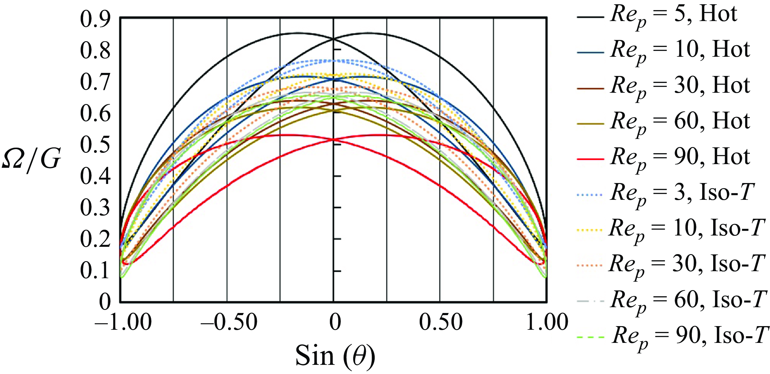
Figure 21. Variation of normalised angular velocity with the orientation for a hot prolate particle ( ${Gr}=80$
, solid lines) and an isothermal particle (dashed lines).
${Gr}=80$
, solid lines) and an isothermal particle (dashed lines).
5. Conclusions
In this work, the dynamic behaviour of prolate particles in isothermal and non-isothermal shear flows is studied. The results reveal that particle inertia, characterised by the particle Reynolds number, has a significant influence on the particle’s behaviour. In both isothermal and non-isothermal cases, two critical particle Reynolds numbers – a lower and an upper value – have been identified that govern the dynamic behaviour of the particle. In the neutrally buoyant isothermal case, below the first critical $\textit{Re}_p$
, the particle’s equilibrium position is located at the centre of the domain. Then, between the lower and upper critical values, a pitchfork bifurcation occurs, and depending on the initial position, the particle may settle in either the upper or lower half of the domain. Finally, beyond the upper critical
$\textit{Re}_p$
, the particle’s equilibrium position is located at the centre of the domain. Then, between the lower and upper critical values, a pitchfork bifurcation occurs, and depending on the initial position, the particle may settle in either the upper or lower half of the domain. Finally, beyond the upper critical $\textit{Re}_p$
, the equilibrium position returns to the centre.
$\textit{Re}_p$
, the equilibrium position returns to the centre.
For the hot particle, the role of these thresholds is different. For the cases below the first critical $\textit{Re}_p$
, the particle ends up in the upper half of the channel. Next, between the lower and upper critical Reynolds numbers, the particle shifts to a lower transverse position, whose location is almost independent of Reynolds number. The hot particle showed no pitchfork bifurcation in the studied cases. Finally, above the upper threshold, the particle moves to a location close to the channel centre.
$\textit{Re}_p$
, the particle ends up in the upper half of the channel. Next, between the lower and upper critical Reynolds numbers, the particle shifts to a lower transverse position, whose location is almost independent of Reynolds number. The hot particle showed no pitchfork bifurcation in the studied cases. Finally, above the upper threshold, the particle moves to a location close to the channel centre.
The influence of the Grashof number on the final position and orientation of the hot particle has been also investigated, which is found to be more significant at low and moderate Reynolds numbers. Specifically, at $\textit{Re}_p=1$
, four distinct modes of motion are identified as the Grashof number increases: settling on the lower wall (at low
$\textit{Re}_p=1$
, four distinct modes of motion are identified as the Grashof number increases: settling on the lower wall (at low ${Gr}$
), tumbling in the upper half, transitioning to log-rolling and, finally, pure translation near the upper wall. As the Reynolds number increases, the number of possible modes decreases. At high Reynolds numbers (
${Gr}$
), tumbling in the upper half, transitioning to log-rolling and, finally, pure translation near the upper wall. As the Reynolds number increases, the number of possible modes decreases. At high Reynolds numbers ( $\textit{Re}_p=90$
), we may end up in a single mode of rotation as observed for
$\textit{Re}_p=90$
), we may end up in a single mode of rotation as observed for ${Gr}=80$
. Moreover, increasing the Grashof number shifts the particle closer to the upper wall due to stronger buoyancy effects.
${Gr}=80$
. Moreover, increasing the Grashof number shifts the particle closer to the upper wall due to stronger buoyancy effects.
The effect of initial orientation on the particle’s final state has been also examined. This influence is more significant at lower Grashof numbers and can result in different modes of motion and final locations. However, above a certain Grashof number (e.g. ${Gr}=50$
for
${Gr}=50$
for $\textit{Re}_p=1$
), the initial orientation no longer affects the particle’s final mode. The effect of initial orientation becomes less pronounced at higher Reynolds numbers. Additionally, when investigating the effect of the particle’s initial position, it was found that a pitchfork bifurcation does not occur for the hot particle. The particle consistently reaches the same final location, regardless of its starting position. As the particle approaches the upper wall, the influence of the Grashof number weakens compared with the hydrodynamic forces, making it less effective at pushing the particle further upwards. At a specific Grashof number (
$\textit{Re}_p=1$
), the initial orientation no longer affects the particle’s final mode. The effect of initial orientation becomes less pronounced at higher Reynolds numbers. Additionally, when investigating the effect of the particle’s initial position, it was found that a pitchfork bifurcation does not occur for the hot particle. The particle consistently reaches the same final location, regardless of its starting position. As the particle approaches the upper wall, the influence of the Grashof number weakens compared with the hydrodynamic forces, making it less effective at pushing the particle further upwards. At a specific Grashof number ( ${Gr}=80$
), as the Reynolds number increases, it was observed that the rotation period of the tumbling motion increases up to the first critical Reynolds number. It then remains constant between the two
${Gr}=80$
), as the Reynolds number increases, it was observed that the rotation period of the tumbling motion increases up to the first critical Reynolds number. It then remains constant between the two $\textit{Re}_p$
thresholds before increasing again beyond the upper critical Reynolds number. In all cases, the rotation period is longer than that predicted theoretically by Jeffery. Interestingly, we observed that the rotational speed of the heated particle exceeds that of the isothermal particle, a result of secondary flows induced by heat convection. In the range between the two critical Reynolds numbers, the hot particle shifts closer to the centreline compared with a neutrally buoyant isothermal particle. This behaviour can be attributed to the enhanced Lighthill–Auton lift force. However, to identify the exact cause of this phenomenon, further in situ analysis is needed, which will be conducted in our future work.
$\textit{Re}_p$
thresholds before increasing again beyond the upper critical Reynolds number. In all cases, the rotation period is longer than that predicted theoretically by Jeffery. Interestingly, we observed that the rotational speed of the heated particle exceeds that of the isothermal particle, a result of secondary flows induced by heat convection. In the range between the two critical Reynolds numbers, the hot particle shifts closer to the centreline compared with a neutrally buoyant isothermal particle. This behaviour can be attributed to the enhanced Lighthill–Auton lift force. However, to identify the exact cause of this phenomenon, further in situ analysis is needed, which will be conducted in our future work.
These findings highlight the increased complexity of the particle’s dynamic behaviour when heat transfer is introduced, as the interplay between various phenomena becomes significantly more intricate. Further investigations are required to better understand the precise mechanisms behind this observation and to explore the effects of additional parameters, such as wall influence, density ratio and confinement ratio. Overall, this study provides insights into the behaviour of thermally active particles and their equilibrium positions in shear flows, which could pave the way for novel applications concerning, for instance, particle–particle separation techniques.
Supplementary movies
Supplementary movies are available at https://doi.org/10.1017/jfm.2025.10280.
Acknowledgements
The authors gratefully acknowledge the Gauss Centre for Supercomputing e.V. (www.gauss-centre.eu) for funding this project by providing computing time on the GCS Supercomputer SuperMUC-NG at Leibniz Supercomputing Centre (www.lrz.de).
Funding
Deutsche Forschungsgemeinschaft (DFG, German Research Foundation) within Project number 465872891.
Declaration of interests
The authors report no conflict of interest.
Data availability statement
The data from this study are available upon request.
Appendix A. Validation of computational methodology
To validate the present computational method, a series of test cases are first modelled. All simulations rely on our in-house hybrid LBM/FD solver called ALBORZ and compared with benchmark solutions. These test cases include: (i) rotation of prolate and oblate spheroids in shear flows; (ii) motion of a single sphere in shear flows; and (iii) sedimentation of cold and hot spherical particles.
A.1. Rotation of a spheroidal particle in low Reynolds number shear flows
To validate the code for non-spherical particles, the rotation of a neutrally buoyant spheroidal particle in a low-Reynolds-number shear flow between two oppositely moving plates is considered. Two cases are investigated: one involving an oblate spheroid and the other a prolate spheroid. In both cases, a cubic domain with a side length of $100\, \text{mm}$
is used, containing a fluid with a density of
$100\, \text{mm}$
is used, containing a fluid with a density of $10^3 \, \text{kg}\,{\rm m}^{-3}$
and a kinematic viscosity of
$10^3 \, \text{kg}\,{\rm m}^{-3}$
and a kinematic viscosity of $10^{-6}\, \text{m}^2\text{s}^{-1}$
. The particle is initially positioned at the centre of the domain. In the first case, an oblate spheroid with a major radius of
$10^{-6}\, \text{m}^2\text{s}^{-1}$
. The particle is initially positioned at the centre of the domain. In the first case, an oblate spheroid with a major radius of $a = 14.44\,\text{mm}$
and minor radius of
$a = 14.44\,\text{mm}$
and minor radius of $b = 4.81\,\text{mm}$
(aspect ratio
$b = 4.81\,\text{mm}$
(aspect ratio $=3$
) is used, with the grid size set to 100
$=3$
) is used, with the grid size set to 100 $\times$
100
$\times$
100 $\times$
100. In the second case, a prolate spheroid with a minor radius of
$\times$
100. In the second case, a prolate spheroid with a minor radius of $b = 3.72\,\text{mm}$
and a major radius of
$b = 3.72\,\text{mm}$
and a major radius of $a = 4.96\,\text{mm}$
(aspect ratio
$a = 4.96\,\text{mm}$
(aspect ratio $= 4/3$
) is examined, and a domain with a grid resolution of 121
$= 4/3$
) is examined, and a domain with a grid resolution of 121 $\times$
121
$\times$
121 $\times$
121 is selected. These parameters match those used in the previous study of Eshghinejadfard, Zhao & Thévenin (Reference Eshghinejadfard, Zhao and Thévenin2018).
$\times$
121 is selected. These parameters match those used in the previous study of Eshghinejadfard, Zhao & Thévenin (Reference Eshghinejadfard, Zhao and Thévenin2018).
Both oblate and prolate spheroids begin to rotate and eventually reach a periodic rotational behaviour. There is no constraint implemented to prevent particle translation within the solver. However, its centre remains at the same position throughout the simulation due to the nature of a pure shear flow. Figures 22 and 23 display the normalised angular velocity ( $\Omega /G$
) in the inertial coordinate system as a function of non-dimensional time (
$\Omega /G$
) in the inertial coordinate system as a function of non-dimensional time ( $tG$
) for oblate and prolate particles, respectively. Under the influence of shear flow, the particle undergoes periodic rotation, reaching its maximum rotation rate when oriented perpendicular to the walls and its minimum rotation rate when aligned parallel to the walls. The present results show excellent agreement with the analytical solution of Jeffery (Reference Jeffery1922) in the low-Reynolds-number regime, demonstrating the model’s capability to accurately predict the motion of spheroidal particles.
$tG$
) for oblate and prolate particles, respectively. Under the influence of shear flow, the particle undergoes periodic rotation, reaching its maximum rotation rate when oriented perpendicular to the walls and its minimum rotation rate when aligned parallel to the walls. The present results show excellent agreement with the analytical solution of Jeffery (Reference Jeffery1922) in the low-Reynolds-number regime, demonstrating the model’s capability to accurately predict the motion of spheroidal particles.
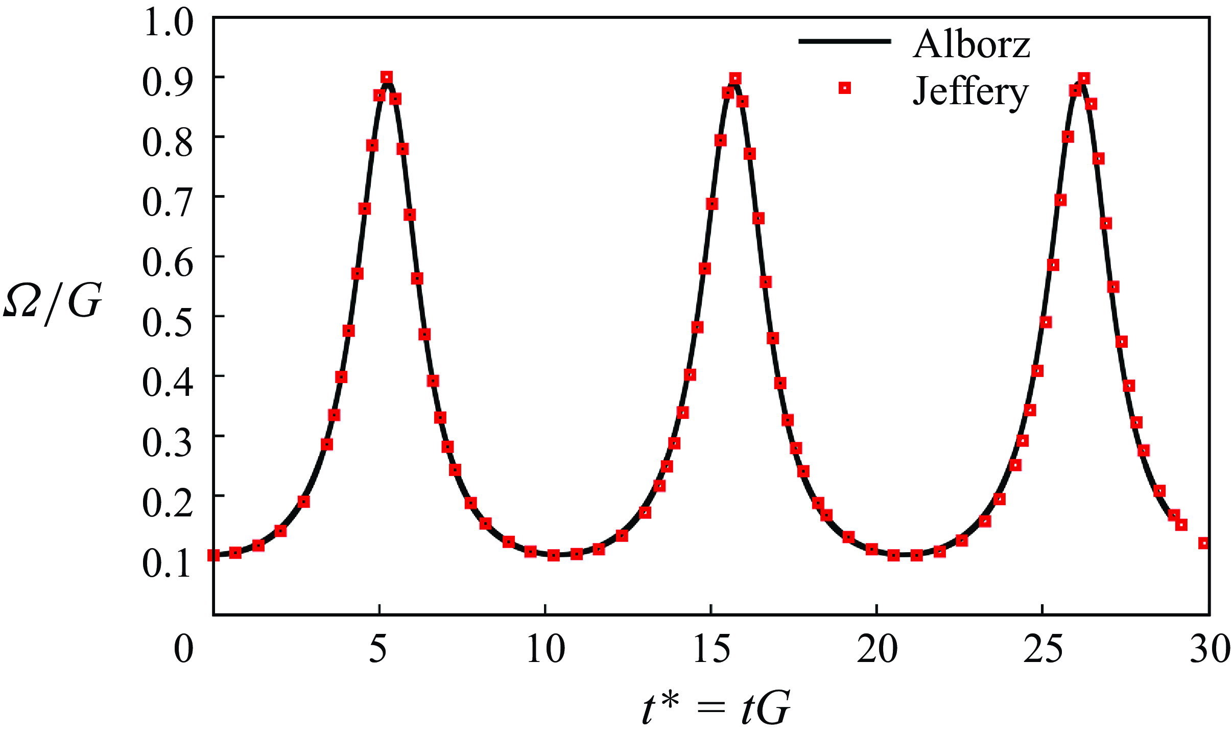
Figure 22. Normalised angular rotation velocity versus non-dimensional time for an oblate spheroid in a Couette flow predicted numerically by ALBORZ (line) and compared with the analytical solution of Jeffery (Reference Jeffery1922) (symbols).
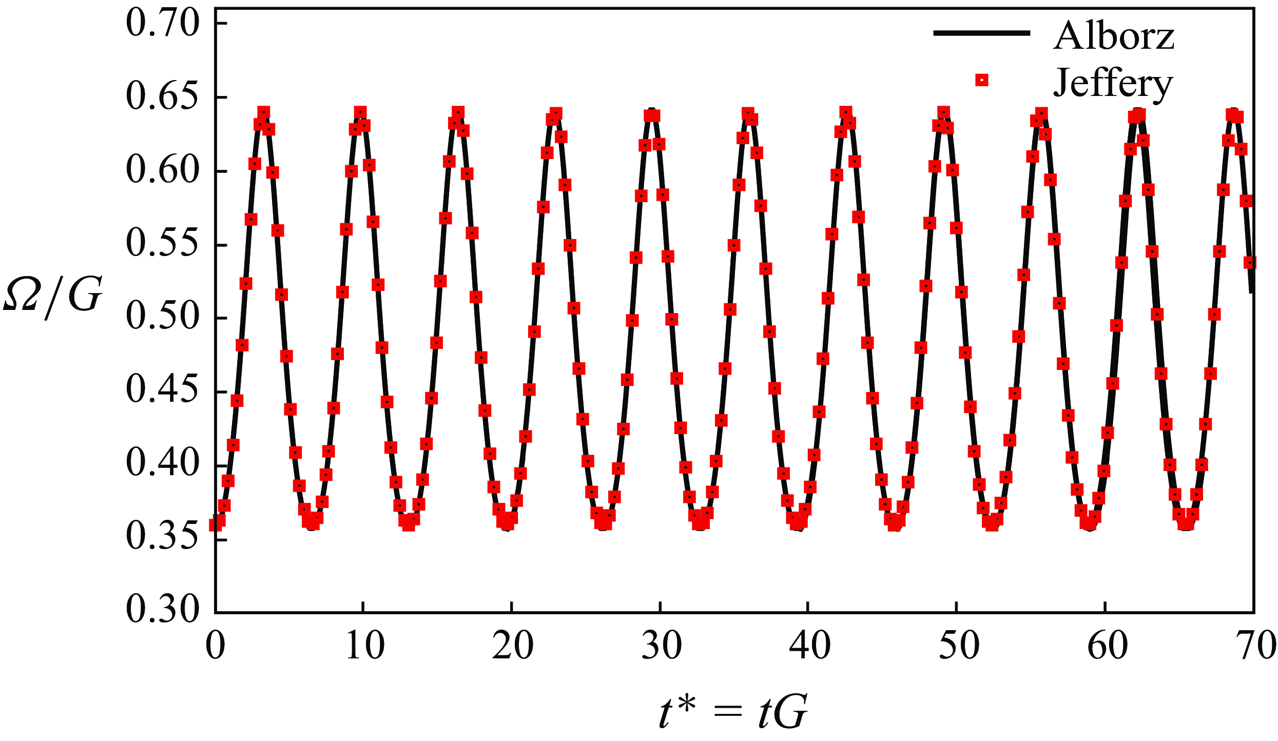
Figure 23. Normalised angular rotation velocity versus non-dimensional time for a prolate spheroid in a Couette flow predicted numerically by ALBORZ (line) and compared with the analytical solution of Jeffery (Reference Jeffery1922) (symbols).
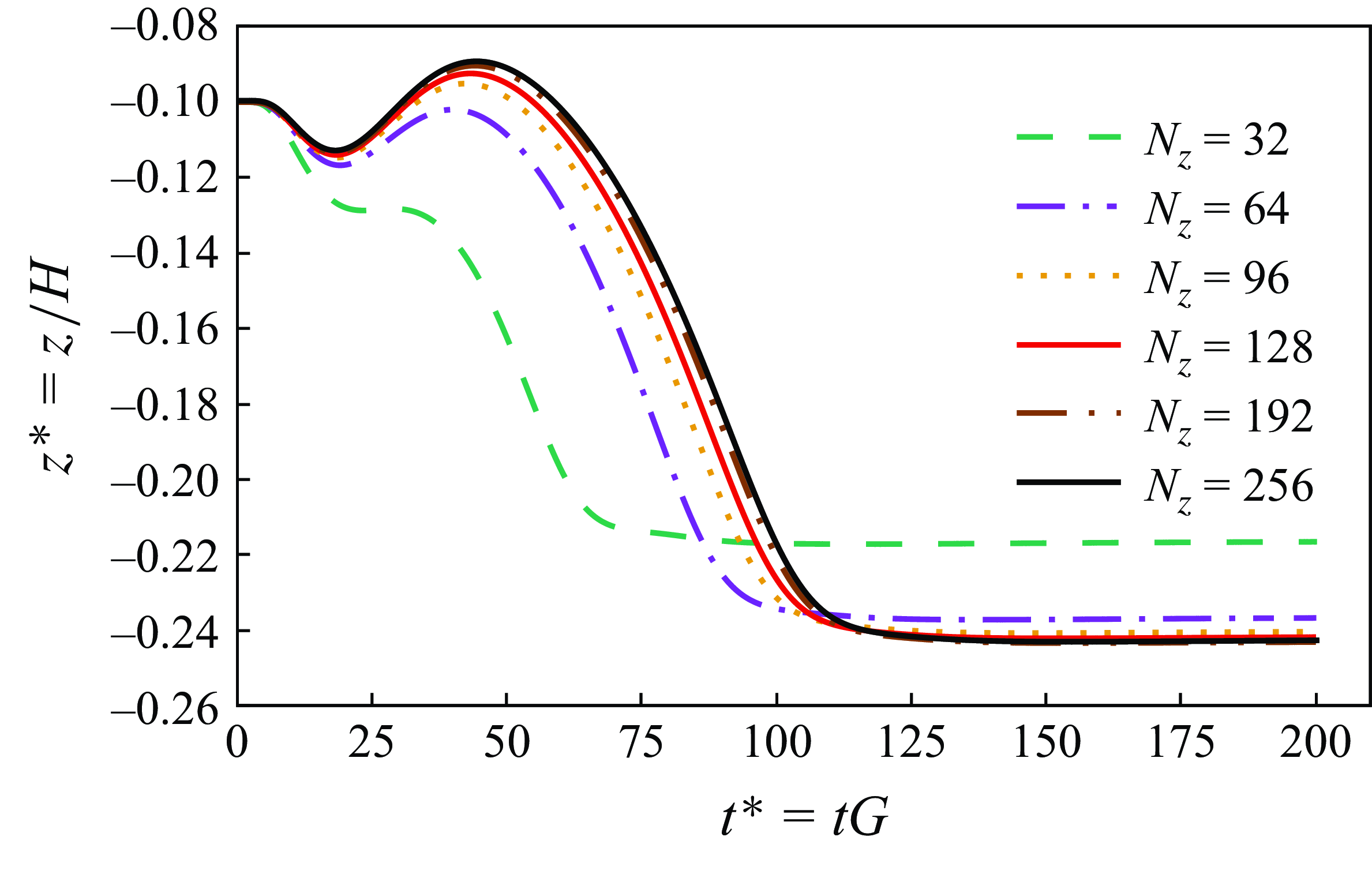
Figure 24. Grid independence study for a spherical particle in a shear flow at $\textit{Re}_p = 30$
.
$\textit{Re}_p = 30$
.
A.2. Dynamic behaviour of a spherical particle in a shear flow
In this part, the dynamic behaviour of a neutrally buoyant spherical particle in a shear flow between two parallel plates is analysed. The schematic and geometric details of the set-up are illustrated in figure 1. The confinement ratio is set to $K = {r_p}/{H} = 0.2$
. The particle is initially positioned off-centre at
$K = {r_p}/{H} = 0.2$
. The particle is initially positioned off-centre at $z^*_0 = -0.1$
, and its migration trajectory is studied for two particle Reynolds numbers of
$z^*_0 = -0.1$
, and its migration trajectory is studied for two particle Reynolds numbers of $\textit{Re}_p= 3$
and 30. The surrounding fluid is at rest and the process is initiated by moving walls. The particle experiences both rotation and translation during the simulation.
$\textit{Re}_p= 3$
and 30. The surrounding fluid is at rest and the process is initiated by moving walls. The particle experiences both rotation and translation during the simulation.
After conducting a grid independence study, a grid size of $N_x\times N_y\times N_z =240 \times 120 \times 120$
was found to be satisfactory for
$N_x\times N_y\times N_z =240 \times 120 \times 120$
was found to be satisfactory for $\textit{Re}_p = 3$
, while a grid size of
$\textit{Re}_p = 3$
, while a grid size of $512 \times 256 \times 256$
was used for
$512 \times 256 \times 256$
was used for $\textit{Re}_p = 30$
. Figure 24 presents the results of this grid independence study for
$\textit{Re}_p = 30$
. Figure 24 presents the results of this grid independence study for $\textit{Re}_p = 30$
. It is observed that the selected mesh size is adequate for extracting output data, as the differences observed between
$\textit{Re}_p = 30$
. It is observed that the selected mesh size is adequate for extracting output data, as the differences observed between $N_z=192$
and
$N_z=192$
and $N_z=256$
are minute.
$N_z=256$
are minute.
Figure 25 shows the particle trajectory at different particle Reynolds numbers as a function of non-dimensional time. The results are compared wherever possible with those of Fox et al. (Reference Fox, Schneider and Khair2021) (obtained by LBM) and Lauricella et al. (Reference Lauricella, Naderi, Zhou, Papautsky and Peng2024) (relying on SPH). For both Reynolds numbers, the particle begins to move and rotate freely, eventually reaching an equilibrium position in the $z$
-direction. For
$z$
-direction. For $\textit{Re}_p = 3$
, the equilibrium position is at the centre of the channel,
$\textit{Re}_p = 3$
, the equilibrium position is at the centre of the channel, $(z=0)$
, regardless of the initial transverse location. The results obtained with ALBORZ show very good agreement with those from Fox et al. (Reference Fox, Schneider and Khair2021) and Lauricella et al. (Reference Lauricella, Naderi, Zhou, Papautsky and Peng2024). Still, Lauricella et al. (Reference Lauricella, Naderi, Zhou, Papautsky and Peng2024) reports a small drop in
$(z=0)$
, regardless of the initial transverse location. The results obtained with ALBORZ show very good agreement with those from Fox et al. (Reference Fox, Schneider and Khair2021) and Lauricella et al. (Reference Lauricella, Naderi, Zhou, Papautsky and Peng2024). Still, Lauricella et al. (Reference Lauricella, Naderi, Zhou, Papautsky and Peng2024) reports a small drop in $z^*$
immediately after the start of the simulation, which is not observed in our results nor in those of Fox et al. (Reference Fox, Schneider and Khair2021).
$z^*$
immediately after the start of the simulation, which is not observed in our results nor in those of Fox et al. (Reference Fox, Schneider and Khair2021).
For $\textit{Re}_p = 30$
, the particle migrates to
$\textit{Re}_p = 30$
, the particle migrates to $z^* = \pm 0.24$
, corresponding to a bifurcation of the equilibrium position. In this case, the final location of the particle depends on its initial position. Due to symmetry, a particle with
$z^* = \pm 0.24$
, corresponding to a bifurcation of the equilibrium position. In this case, the final location of the particle depends on its initial position. Due to symmetry, a particle with $z^*_0 \lt 0$
moves to the equilibrium position
$z^*_0 \lt 0$
moves to the equilibrium position $z^* = -0.24$
(this is the case shown in figure 25), while a particle with
$z^* = -0.24$
(this is the case shown in figure 25), while a particle with $z^*_0 \gt 0$
moves to the equilibrium position
$z^*_0 \gt 0$
moves to the equilibrium position $z^*= +0.24$
. For this higher value of the particle Reynolds number,
$z^*= +0.24$
. For this higher value of the particle Reynolds number, $\textit{Re}_p = 30$
, large differences are observed among the different studies. While the final equilibrium position is similar across all models, the time and the path taken to reach this position differ noticeably. Regarding Fox et al. (Reference Fox, Schneider and Khair2021), the discrepancy can be attributed to the coarser grid used in their study (
$\textit{Re}_p = 30$
, large differences are observed among the different studies. While the final equilibrium position is similar across all models, the time and the path taken to reach this position differ noticeably. Regarding Fox et al. (Reference Fox, Schneider and Khair2021), the discrepancy can be attributed to the coarser grid used in their study ( $N_x\times N_y\times N_z =128 \times 64 \times 64$
) as the importance of a sufficiently fine mesh is evident from figure 24. Additionally, Fox et al. (Reference Fox, Schneider and Khair2021) used a single relaxation time LBM while we employ an enhanced LBM collision operator that eliminates cubic errors in the deviatoric components of the viscous stress tensor, resulting in more accurate outcomes. Lauricella et al. (Reference Lauricella, Naderi, Zhou, Papautsky and Peng2024) attributed the difference in their observations to those from Fox et al. (Reference Fox, Schneider and Khair2021) to some degree of compressibility present in their SPH model. Based on the previous sections and on the grid independence test, we feel confident that the results shown for ALBORZ in figure 25 are reliable. Additionally, the later part of this work concentrates on the final equilibrium position reached by the particle, and those remain very similar across all studies.
$N_x\times N_y\times N_z =128 \times 64 \times 64$
) as the importance of a sufficiently fine mesh is evident from figure 24. Additionally, Fox et al. (Reference Fox, Schneider and Khair2021) used a single relaxation time LBM while we employ an enhanced LBM collision operator that eliminates cubic errors in the deviatoric components of the viscous stress tensor, resulting in more accurate outcomes. Lauricella et al. (Reference Lauricella, Naderi, Zhou, Papautsky and Peng2024) attributed the difference in their observations to those from Fox et al. (Reference Fox, Schneider and Khair2021) to some degree of compressibility present in their SPH model. Based on the previous sections and on the grid independence test, we feel confident that the results shown for ALBORZ in figure 25 are reliable. Additionally, the later part of this work concentrates on the final equilibrium position reached by the particle, and those remain very similar across all studies.
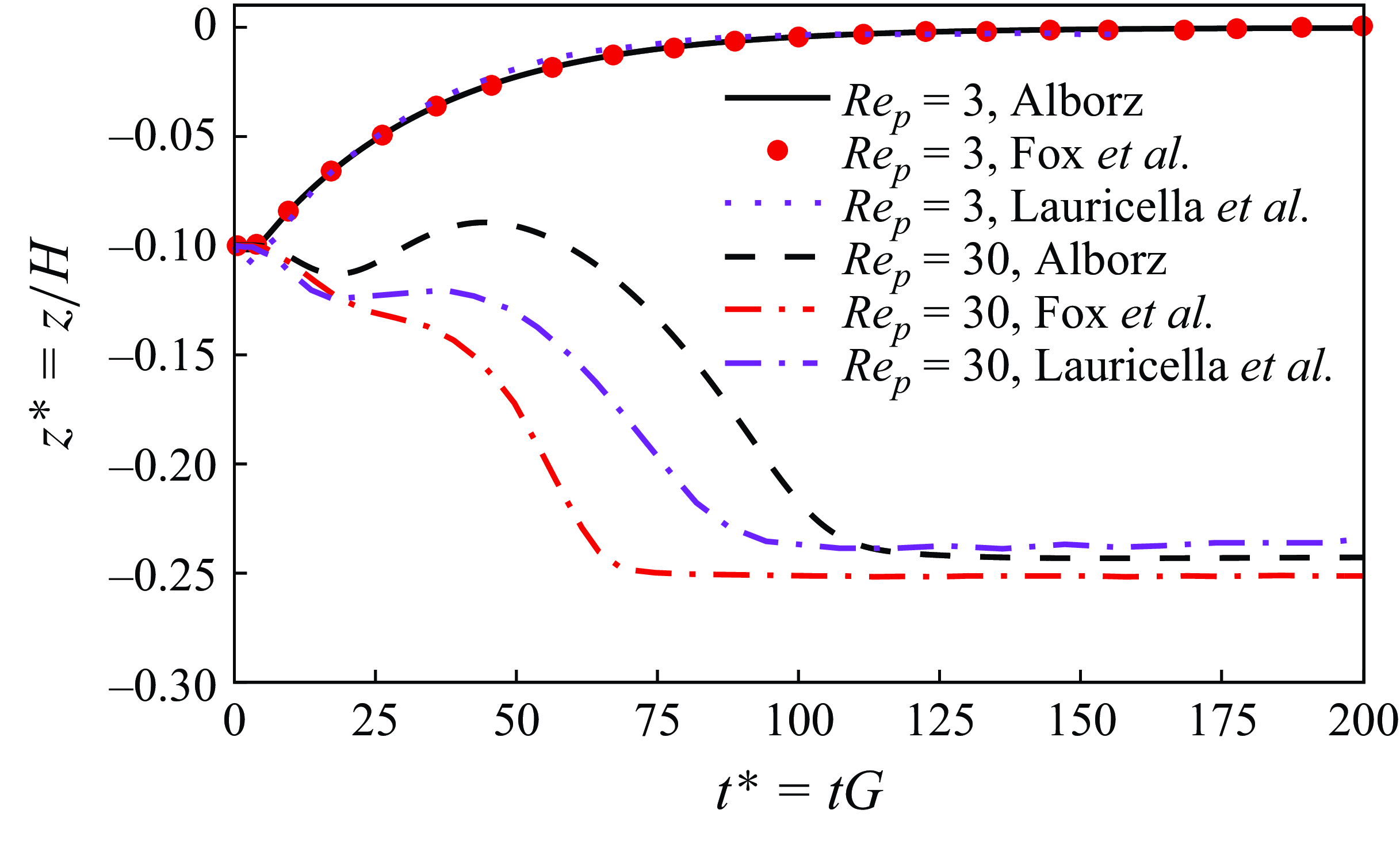
Figure 25. Trajectory of a spherical particle in a shear flow versus non-dimensional time at two particle Reynolds numbers of $\textit{Re}_p = 3$
and 30. Our own results obtained with ALBORZ are compared with those published by Fox et al. (Reference Fox, Schneider and Khair2021) (obtained by LBM) and Lauricella et al. (Reference Lauricella, Naderi, Zhou, Papautsky and Peng2024) (relying on SPH).
$\textit{Re}_p = 3$
and 30. Our own results obtained with ALBORZ are compared with those published by Fox et al. (Reference Fox, Schneider and Khair2021) (obtained by LBM) and Lauricella et al. (Reference Lauricella, Naderi, Zhou, Papautsky and Peng2024) (relying on SPH).
A.3. Sedimentation of a non-isothermal sphere
Up to now, all simulations did not consider temperature as an important variable, being isothermal. In this part, we investigate the sedimentation of hot and cold spheres within a closed enclosure to validate the thermal solver. The sphere is subject to the gravitational force, and the Boussinesq approximation is used to capture the effects of natural convection around the particle. It is important to note that the Boussinesq force is not applied to the virtual Eulerian nodes of the fluid domain located within the particle itself. The simulation domain is illustrated in figure 26. The fluid density is $\rho _f=10^{3} \, \text{kg}\,\rm {m}^{-3}$
, with a kinematic viscosity of
$\rho _f=10^{3} \, \text{kg}\,\rm {m}^{-3}$
, with a kinematic viscosity of $10^{-4} \, \text{m}^{2}\textrm{s}^{-1}$
. The density ratio between the particle and the fluid is set to
$10^{-4} \, \text{m}^{2}\textrm{s}^{-1}$
. The density ratio between the particle and the fluid is set to $\rho _r=\rho _p/\rho _f=1.1$
, while the ratio of specific heat capacity is
$\rho _r=\rho _p/\rho _f=1.1$
, while the ratio of specific heat capacity is $C_{p,p}/C_{p,f}=1.0$
. The fluid Prandtl number is chosen as
$C_{p,p}/C_{p,f}=1.0$
. The fluid Prandtl number is chosen as $1.0$
, and simulations are performed for Grashof numbers
$1.0$
, and simulations are performed for Grashof numbers ${Gr} = 100$
and
${Gr} = 100$
and ${Gr} = -100$
. The LBM relaxation time is set to
${Gr} = -100$
. The LBM relaxation time is set to $\tau =0.6$
. The enclosure boundaries are maintained at a constant temperature, equal to the initial temperature of the fluid. In this part, the non-dimensional temperature of the solid is set to
$\tau =0.6$
. The enclosure boundaries are maintained at a constant temperature, equal to the initial temperature of the fluid. In this part, the non-dimensional temperature of the solid is set to $T^* = 1$
for
$T^* = 1$
for $\text{Gr} = 100$
and
$\text{Gr} = 100$
and $T^* = -1$
for
$T^* = -1$
for $\text{Gr} = -100$
.
$\text{Gr} = -100$
.
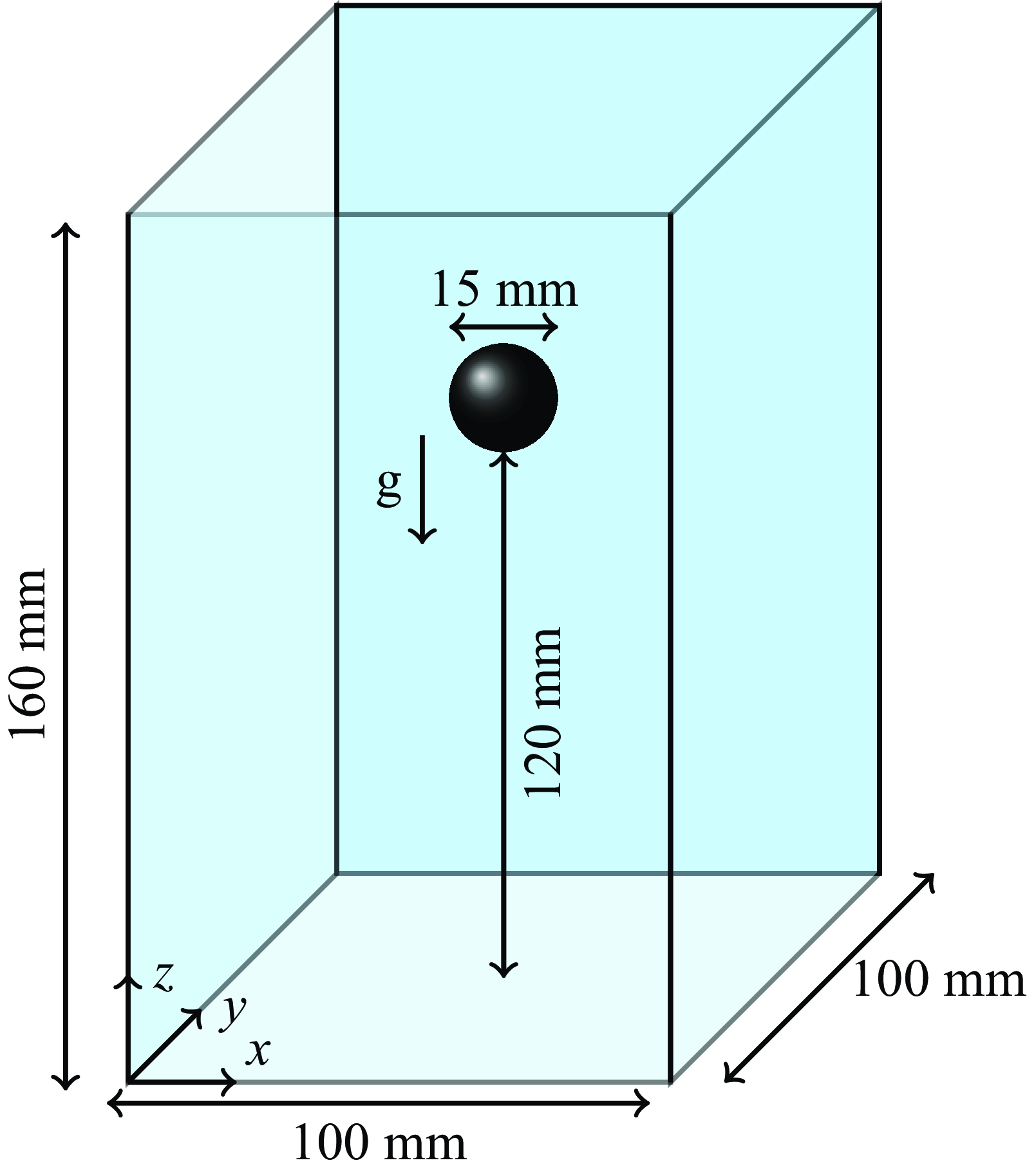
Figure 26. Schematic of the set-up for the sedimentation of a single spherical particle.
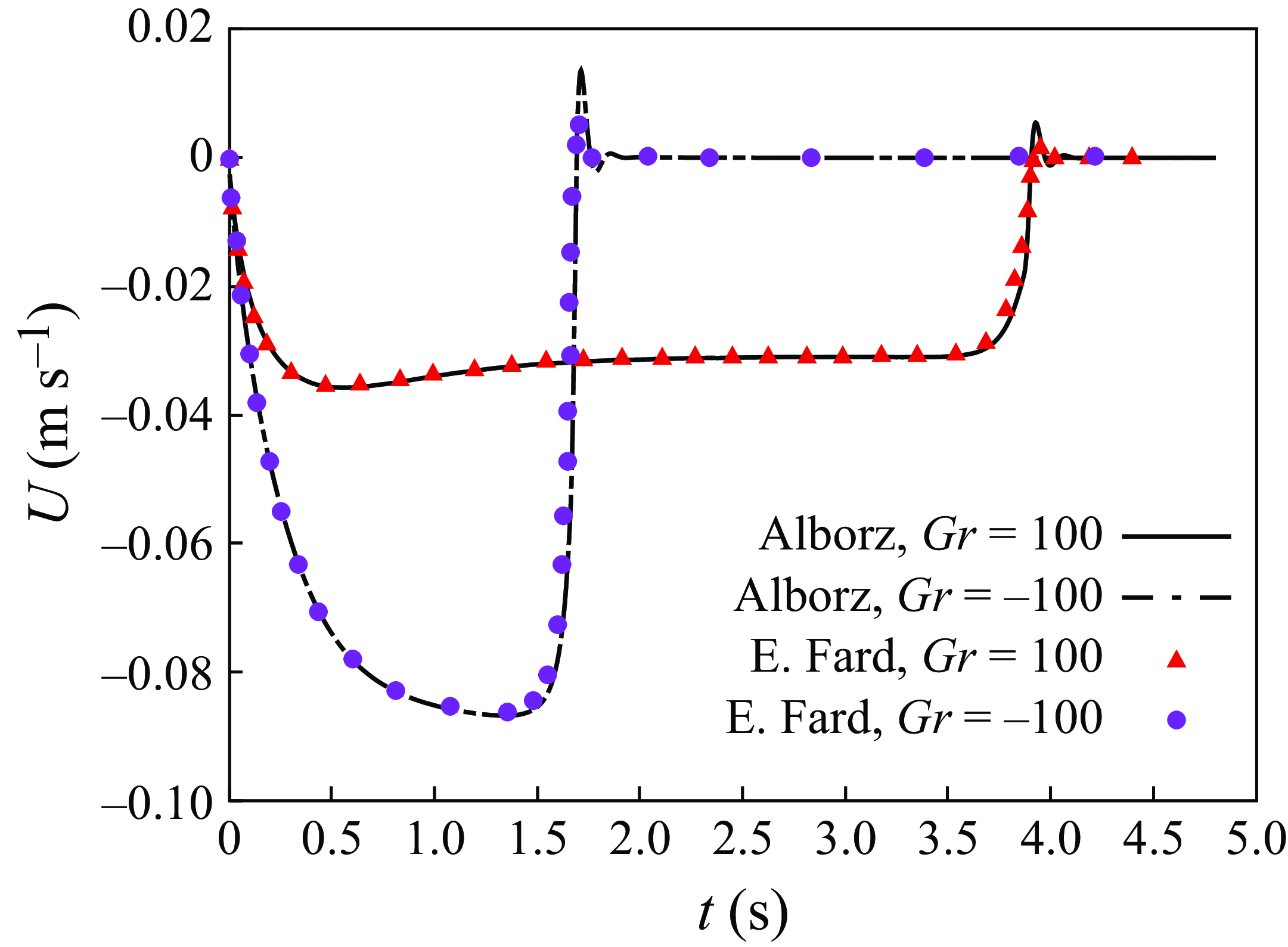
Figure 27. Settling velocity of a thermal particle (lines) compared with the previous study of Eshghinejadfard & Thévenin (Reference Eshghinejadfard and Thévenin2016) (symbols) for two different Grashof numbers of ${Gr} = 100$
and
${Gr} = 100$
and ${Gr} = -100$
.
${Gr} = -100$
.
The simulation results are shown in figure 27 and compared with the data from Eshghinejadfard & Thévenin (Reference Eshghinejadfard and Thévenin2016). As expected, particle sedimentation is influenced by both upward buoyancy force and downward gravitational force. The comparisons show a very good agreement between the current study and the published data. In the case of ${Gr} = 100$
, the drag force induced by natural convection and upward fluid motion reduces the particle terminal velocity. This reduction occurs because the hot fluid surrounding the particle starts moving upwards, counteracting the downwards motion of the particle due to its higher density. Conversely, for
${Gr} = 100$
, the drag force induced by natural convection and upward fluid motion reduces the particle terminal velocity. This reduction occurs because the hot fluid surrounding the particle starts moving upwards, counteracting the downwards motion of the particle due to its higher density. Conversely, for ${Gr} = -100$
, where the particle is colder than the surrounding fluid, the naturally convected flow moves downwards, accelerating the particle and consequently increasing its terminal velocity before collision with the bottom wall.
${Gr} = -100$
, where the particle is colder than the surrounding fluid, the naturally convected flow moves downwards, accelerating the particle and consequently increasing its terminal velocity before collision with the bottom wall.


 Open access