


1. Introduction
The issue of cavitation erosion is prevalent in the fields of shipbuilding and ocean engineering, with the primary concern being the collapse and destruction of cavitation bubbles adjacent to the wall surface (Klaseboer et al. Reference Klaseboer, Hung, Wang, Wang, Khoo, Boyce, Debono and Charlier2005; Zhang et al. Reference Zhang, Cui, Cui and Wang2015; Liu et al. Reference Liu, Yao, Liu and Yu2018a ; Tian et al. Reference Tian, Liu, Zhang, Tao and Chen2020; Li et al. Reference Li, Zhang, Cui, Li and Liu2023; Zhang et al. Reference Zhang, Li, Xu, Pei, Li and Liu2024). The presence of a wall surface disrupts the symmetrical boundary of a bubble and causes a jet to form towards the wall during the collapse process (Plesset & Chapman Reference Plesset and Chapman1971; Blake & Gibson Reference Blake and Gibson1987; Liu et al. Reference Liu, Gan, Wang and Zhang2021). The jet impacts the wall, resulting in high impulsive pressure. It then propagates along the boundary to cause high wall shear stress (Zeng et al. Reference Zeng, Gonzalez-Avila, Dijkink, Koukouvinis, Gavaises and Ohl2018, Reference Zeng, An and Ohl2022; Park et al. Reference Park, Phan, Nguyen, Duy, Nguyen and Park2024). Additionally, during the pulsation process, the pulsating pressure emitted by the bubble focuses on the wall to generate a high-pressure region (Lechner et al. Reference Lechner, Koch, Lauterborn and Mettin2017; Veysset et al. Reference Veysset, Gutiérrez-Hernández, Dresselhaus-Cooper, De Colle, Kooi, Nelson, Quinto-Su and Pezeril2018). The impact of the jet and the pressure focus are two primary causes of cavitation erosion in propellers (Reuter, Deiter & Ohl Reference Reuter, Deiter and Ohl2022a ). Regarding how to reduce cavitation erosion, one method is to select new materials that are resistant to erosion and compression (Cheng, Kwok & Man Reference Cheng, Kwok and Man2001; Kwok et al. Reference Kwok, Man, Cheng and Lo2016), and another method is to adjust the flow field to weaken the jet of cavitation bubbles (Gonzalez-Avila et al. Reference Gonzalez-Avila, Nguyen, Arunachalam, Domingues, Mishra and Ohl2020; Kadivar et al. Reference Kadivar, el Moctar, Skoda and Löschner2021). A novel approach was discussed regarding whether the viscous layer on the surface has the function of resisting cavitation erosion. That is, an oil layer is attached to the wall surface to investigate the effect of the viscous layer on the bubble dynamics and wall pressure load characteristics.
Cavitation bubbles interact with wall-attached viscous oil layers in two aspects: the bubble–wall coupling and the bubble–immiscible-interface coupling system. Numerous research findings have examined pulsating bubbles near the wall, with detailed analyses of the mechanisms underlying bubble collapse jets and other related phenomena. Following systematic experiments conducted by Philipp & Lauterborn (Reference Philipp and Lauterborn1998) on cavitation bubble-induced pitting of metallic materials, the issue of near-wall cavitation damage has regained attention from scholars. Dular et al. (Reference Dular2019) has emphasised the significant damage inflicted on material surfaces by microjets and bubble annular collapses. More recently, Reuter et al. (Reference Reuter, Deiter and Ohl2022a ) found, through high-speed imaging and shadowgraphy of the shock-wave fronts, that the damage to the material surface caused by cavitation bubbles can be categorised mainly into two forms: erosion damage resulting from self-focusing of non-axisymmetric collapsing shock waves and extrusion damage caused by high-speed jets and annular collapse of bubbles.
For the bubble–immiscible-interface interaction, recently, numerous scholars have delved into the dynamics of bubbles at the interface of two phases in a planar configuration. Freund, Shukla & Evan (Reference Freund, Shukla and Evan2009) simulated the behaviour of shock-wave-induced bubble jets entering different viscosity media and provide theoretical predictions of the jet penetration depth in viscous media. Liu et al. (Reference Liu, Zhang, Tian and Wang2019) and Su et al. (Reference Su, Liu, Tian, Zhang and Zhang2023) examined bubble oscillations at interfaces of two fluids. Han et al. (Reference Han, Zhang, Tan and Li2022) conducted experiments on bubble generation near the water–oil interface induced by electric sparks, uncovering two mechanisms of bubble-induced water–oil mixing: bubble transport via high-speed jets and jet breakup. However, in these studies, the oil–water interfaces were free-floating. When the viscous oil layer adheres to a rigid wall, the fluid dynamics becomes even more intricate.
The dynamics and jetting behavior of bubbles exhibit greater complexity when an immiscible liquid-liquid interface exists between the bubble and the wall surface, thereby substantially affecting the bubble’s interaction with the wall. Two recent noteworthy studies involve the Ohl, Reese & Ohl (Reference Ohl, Reese and Ohl2024) investigation into laser cavitation bubbles near a flat oil layer and the Ren et al. (Reference Ren, Han, Zeng, Sun, Tagawa, Zuo and Liu2023) examination of hemispherical low-viscosity oil droplets attached to a surface. While primarily categorising various forms of bubble entrapment in oil, these studies did not delve into characteristics such as bubble jets, wall pressure load, shear stress, and the influence of viscous fluid on bubble migration – factors crucial in cavitation erosion or bubble cleaning. Addressing these scientific gaps, this paper conducts a numerical analysis of the changes in bubble migration, wall pressure load and viscous fluid shear stress, across varying thicknesses and viscosities of viscous oil layers adhering to the wall.
This study employs a well-established Eulerian finite element method(EFEM) to develop a model for the interaction between bubbles and viscous oil layers attached to a rigid wall. To further validate the numerical model, experiments are conducted on a laser-induced cavitation bubble platform developed in-house (Li et al. Reference Li, Zhao, Zhang and Han2024; Zhang et al. Reference Zhang, Zhang, Zhang, Long, Han, Liu, Ohl and Li2025). In § 2, we provide a concise overview of the numerical and physical models introduced in this paper, followed by a comparison between the numerical model and experimental results. Section 3 entails a parametric investigation using the numerical model, meticulously examining the variations in physical parameters such as migration and wall pressure load and elucidating the underlying physical mechanisms. In § 4, qualitative conclusions are drawn, along with the derivation of quantitative parameters pertaining to the impact of the viscous oil layer on bubble dynamics.
2. Theoretical models and methodology
2.1. Experimental set-up and governing equations
As shown in figure 1(d), a dynamic system of oscillating bubbles near a rigid wall with an attached viscous oil layer is established in an axisymmetric coordinate system. A silicone oil with variable viscosity is used to act as the viscous oil layer. The origin of the coordinate axes is located on the rigid wall, with the radial coordinate denoted as $r$
and the axial coordinate as
$r$
and the axial coordinate as $z$
. At the initial moment, there is a viscous oil layer with a thickness of
$z$
. At the initial moment, there is a viscous oil layer with a thickness of $h$
beneath the rigid wall, and the initial distance between the bubble and the wall is denoted as
$h$
beneath the rigid wall, and the initial distance between the bubble and the wall is denoted as $d$
. The rigid wall adopts a no-slip boundary, while the surroundings adopt a non-reflecting boundary condition. This paper simulates the interaction between laser-induced cavitation bubbles and the wall with the viscous oil layer. Due to the small size of the bubbles, the gravity on the bubble–wall–oil system is disregarded. Figure 1(a) shows a schematic diagram of the laser-induced cavitation bubble platform. A pulsed laser (Q-switched Nd:YAG, Nimma 900, pulse duration
$d$
. The rigid wall adopts a no-slip boundary, while the surroundings adopt a non-reflecting boundary condition. This paper simulates the interaction between laser-induced cavitation bubbles and the wall with the viscous oil layer. Due to the small size of the bubbles, the gravity on the bubble–wall–oil system is disregarded. Figure 1(a) shows a schematic diagram of the laser-induced cavitation bubble platform. A pulsed laser (Q-switched Nd:YAG, Nimma 900, pulse duration $8\,{\textrm {ns}}$
, wavelength
$8\,{\textrm {ns}}$
, wavelength $532\, {\textrm {nm}}$
) is utilised to induced cavitation bubbles in a water medium, while a continuous LED lamp serves as a back lighting source for the high-speed camera (Phantom V2012, 180 000 frames per second). An array light source provides additional bottom illumination. A circular ring fabricated from acrylic is affixed to the aluminium plate surface, and the interior of the ring is filled with silicone oil of different viscosities. The thickness of the silicone-oil layer was determined by the height of the acrylic rings. The entire device is submerged in a
$532\, {\textrm {nm}}$
) is utilised to induced cavitation bubbles in a water medium, while a continuous LED lamp serves as a back lighting source for the high-speed camera (Phantom V2012, 180 000 frames per second). An array light source provides additional bottom illumination. A circular ring fabricated from acrylic is affixed to the aluminium plate surface, and the interior of the ring is filled with silicone oil of different viscosities. The thickness of the silicone-oil layer was determined by the height of the acrylic rings. The entire device is submerged in a $10\, {\textrm {cm}}$
cubic glass vessel filled with deionised water at 23
$10\, {\textrm {cm}}$
cubic glass vessel filled with deionised water at 23 $^\circ {\textrm {C}}$
. Cavitation bubbles are generated in the water below the silicone-oil layer.
$^\circ {\textrm {C}}$
. Cavitation bubbles are generated in the water below the silicone-oil layer.
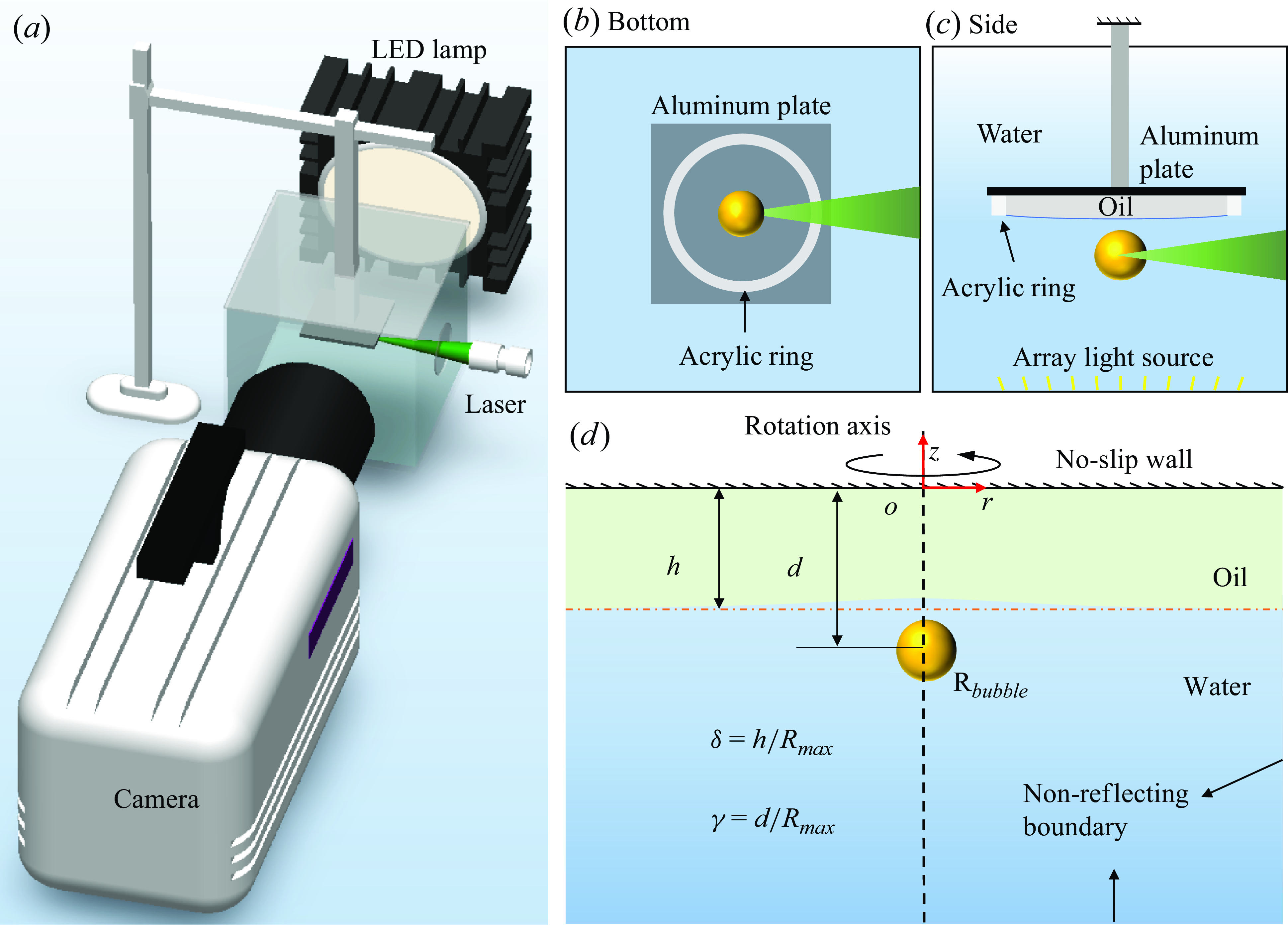
Figure 1. (a) Schematic diagram of the experimental configuration, (b) bottom view, (c) side view, (d) numerical model illustration of the bubble–wall–viscous-oil-layer coupling. Where $R_{bubble}$
is the bubble radius at any moment.
$R_{bubble}$
is the bubble radius at any moment.
This study tackles a typical multiphase flow problem, hence, we utilise the volume of fluid (VOF) (Hirt & Nichols Reference Hirt and Nichols1981) method to manage the multiphase interface. In previous literature, viscous effects were frequently disregarded in bubble dynamics. However, this paper predominantly examines the impact of viscosity in the oil layer on bubble dynamics, thus the fluid viscosity cannot be ignored. The fluid flow adheres to the following equations:
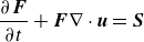
 \begin{equation} \frac {{\partial \boldsymbol{F}}}{{\partial t}} + \nabla \boldsymbol\cdot ( { \boldsymbol{F} \boldsymbol{u}} ) = \boldsymbol{S}, \end{equation}
where $\boldsymbol{F}$
denotes the conserved vector,
$\boldsymbol{F}$
denotes the conserved vector, $\boldsymbol{S}$
stands for the source vector, and
$\boldsymbol{S}$
stands for the source vector, and $\boldsymbol{u}$
represents the velocity of the fluid material. Regarding multiphase flow problems, the following vectors are presented:
$\boldsymbol{u}$
represents the velocity of the fluid material. Regarding multiphase flow problems, the following vectors are presented:
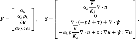 \begin{equation} \boldsymbol {F} = \left [ \begin{array}{c} {\alpha _k}\\ {\alpha _k}{\rho _k}\\ \bar \rho \boldsymbol{u}\\ {\alpha _k}{\rho _k}{e_k} \end{array} \right ] ,\quad \boldsymbol {S} = \left [ \begin{array}{c} {\alpha _k\dfrac {\overline K}{K_k} \nabla \cdot \boldsymbol{u}}\\ {0}\\ { \nabla \cdot (-p \boldsymbol {I}+\boldsymbol{\tau }) + \nabla \cdot \boldsymbol{\psi }}\\ {-\alpha _k p \dfrac {\overline K}{K_k} \nabla \cdot \boldsymbol{u} + \boldsymbol{\tau } : \nabla \boldsymbol{u} + \boldsymbol{\psi } : \nabla \boldsymbol{u}} \end{array} \right ]. \end{equation}
The four components of $\boldsymbol {F}$
, respectively, represent the volume fraction, mass, momentum and internal energy, where subscript
$\boldsymbol {F}$
, respectively, represent the volume fraction, mass, momentum and internal energy, where subscript $k$
denotes the fluid types. This paper considers three types of fluids: water, silicone oil and air. Here,
$k$
denotes the fluid types. This paper considers three types of fluids: water, silicone oil and air. Here, $\alpha$
denotes the volume fraction, defined as the ratio of fluid volume to mesh volume, and in an arbitrary mesh there are
$\alpha$
denotes the volume fraction, defined as the ratio of fluid volume to mesh volume, and in an arbitrary mesh there are $\sum {{\alpha _k}} = 1$
;
$\sum {{\alpha _k}} = 1$
; $\rho$
,
$\rho$
, $t$
and
$t$
and $p$
represent density, time and pressure, respectively, and
$p$
represent density, time and pressure, respectively, and $\bar \rho$
represents the average density of the fluid in the mesh, which is weighted by the density of all fluids,
$\bar \rho$
represents the average density of the fluid in the mesh, which is weighted by the density of all fluids, $\bar \rho = \sum {{\alpha _k}{\rho _k}}$
. Here,
$\bar \rho = \sum {{\alpha _k}{\rho _k}}$
. Here, $K=\rho c^2$
is the fluid bulk modulus, where
$K=\rho c^2$
is the fluid bulk modulus, where $c$
is the sound speed, and the weight bulk modulus can be expressed as
$c$
is the sound speed, and the weight bulk modulus can be expressed as $\bar K= \left(\sum {\alpha _k/K_k}\right)^{-1}$
. The velocity vector is denoted by
$\bar K= \left(\sum {\alpha _k/K_k}\right)^{-1}$
. The velocity vector is denoted by $\boldsymbol{u} = ( {{u_r},{u_z}} )$
. The fluid viscosity is included in the shear stress
$\boldsymbol{u} = ( {{u_r},{u_z}} )$
. The fluid viscosity is included in the shear stress $\boldsymbol{\tau } = \mu [ {\nabla \boldsymbol{u} + \nabla {\boldsymbol{u}^T} - ({2}/{3}) ( {\nabla \cdot \boldsymbol{u}} )\boldsymbol{I}} ]$
, where
$\boldsymbol{\tau } = \mu [ {\nabla \boldsymbol{u} + \nabla {\boldsymbol{u}^T} - ({2}/{3}) ( {\nabla \cdot \boldsymbol{u}} )\boldsymbol{I}} ]$
, where $\mu$
is the dynamic viscosity and
$\mu$
is the dynamic viscosity and $\boldsymbol{I}$
is the normalised tensor. In the conservation of momentum equation
$\boldsymbol{I}$
is the normalised tensor. In the conservation of momentum equation $\boldsymbol{\psi }$
denotes the stress tensor due to surface tension. According to previous literature (Brackbill, Kothe & Zemach Reference Brackbill, Kothe and Zemach1992; Perigaud & Saurel Reference Perigaud and Saurel2005), the tensor can be represented as
$\boldsymbol{\psi }$
denotes the stress tensor due to surface tension. According to previous literature (Brackbill, Kothe & Zemach Reference Brackbill, Kothe and Zemach1992; Perigaud & Saurel Reference Perigaud and Saurel2005), the tensor can be represented as $\boldsymbol{\psi }=\sigma (|\boldsymbol{m}| \boldsymbol{I} -({(\boldsymbol{m} \otimes \boldsymbol{m})}/{|\boldsymbol{m}|}))$
, with the volume fraction gradient
$\boldsymbol{\psi }=\sigma (|\boldsymbol{m}| \boldsymbol{I} -({(\boldsymbol{m} \otimes \boldsymbol{m})}/{|\boldsymbol{m}|}))$
, with the volume fraction gradient $\boldsymbol{m}=\nabla \alpha$
and the surface tension coefficient
$\boldsymbol{m}=\nabla \alpha$
and the surface tension coefficient $\sigma$
. The specific internal energy
$\sigma$
. The specific internal energy $e$
is employed to represent the internal energy per unit mass of the fluid. In the axisymmetric coordinate system,
$e$
is employed to represent the internal energy per unit mass of the fluid. In the axisymmetric coordinate system,
 \begin{equation} \begin{cases} \nabla \cdot \boldsymbol{u} = \dfrac {{\partial {u_r}}}{{\partial r}} + \dfrac {{\partial {u_z}}}{{\partial z}} + \dfrac {{{u_r}}}{r},\\[6pt] \nabla p = \left(\dfrac {{\partial p}}{{\partial r}} , \dfrac {{\partial p}}{{\partial z}}\right). \end{cases} \end{equation}
In this paper, the fluid inside a cavitation bubble is considered a non-condensable gas, and water and silicone oil are treated using the equation of state. Here, we employ the stiffened equation of state (Ivings, Causon & Toro (Reference Ivings, Causon and Toro1998)) to handle gases and liquids:
 \begin{equation} p + \zeta \textit{B} = \rho e ( {\zeta - 1} ) , \end{equation}
where $\zeta$
represents the specific heat ratio of the fluid,
$\zeta$
represents the specific heat ratio of the fluid, ${B}$
is a pressure constant related to the compressibility of the fluid, and
${B}$
is a pressure constant related to the compressibility of the fluid, and $e$
represents the specific internal energy. For non-condensable gas,
$e$
represents the specific internal energy. For non-condensable gas, ${B} = 0$
indicates that the equation transforms into an ideal gas equation of state. According to Tammann’s equation, the fluid sound speed can be obtained as:
${B} = 0$
indicates that the equation transforms into an ideal gas equation of state. According to Tammann’s equation, the fluid sound speed can be obtained as:
 \begin{equation} {c^2} = \dfrac {{{\rm d}p}}{{{\rm d}\rho }} = \dfrac {{\zeta (\textit{B} + p)}}{\rho }. \end{equation}
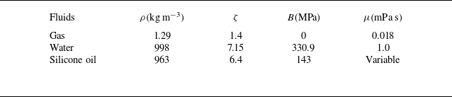
In this paper, the values of the parameters for the three fluids are taken as shown in table 1.
Table 1. Properties of materials in numerical models.
2.2. Eulerian finite element method
The EFEM has found extensive applications in various domains, including underwater explosions (Xu et al. Reference Xu, Tian, Liu and Wang2023; He et al. Reference He, Yan, Lv, Duan and Zhang2024; Qin et al. Reference Qin, Liu, Tian, Liu and Wang2024), multiphase interfaces (Liu et al. Reference Liu, Zhang, Tian and Wang2019; Feng et al. Reference Feng, Liu, Wang, Zhang and Tao2023; Su et al. Reference Su, Liu, Tian, Zhang and Zhang2023; Tang et al. Reference Tang, Tian, Ju, Feng, Zhang and Zhang2023) bubble dynamics and fluid-structure interactions (Liu et al. Reference Liu, Zhang, Miao, Ming and Liu2023, Reference Liu, Liu, Ming, Liu and Zhang2024). The EFEM previously employed by our team was applied mostly in the domain of underwater explosions, disregarding the effects of fluid viscosity and surface tension. In this paper, we have taken viscosity and surface tension into consideration and established a dynamic model of the interaction between bubbles and a rigid wall-attached viscous oil layer. The EFEM employs operator splitting to solve the governing equations in two stages, known as the Lagrangian phase and Eulerian phase. Hence, the equation is decomposed as follows:
 \begin{equation} \dfrac {{\partial {\boldsymbol{F}}}}{{\partial t}} + {\boldsymbol{F}}\nabla \cdot \boldsymbol{u} = \boldsymbol{S} \end{equation}
and
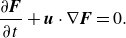 \begin{equation} \dfrac {{\partial \boldsymbol{F}}}{{\partial t}} +\boldsymbol{u} \cdot \nabla \boldsymbol{F} = 0. \end{equation}
The first stage is the Lagrangian phase, within which the source terms are incorporated and (2.6) without convective terms is solved. Thus, no data exchange takes place between adjacent meshes in this step. The meshes are bound to the fluid material and follow the deformation of the fluid, and this stage can be solved by adopting the finite element method. Next, in the second stage, we solve (2.7), considering the information exchange between adjacent meshes, namely transport, which is called the Eulerian phase. A more figurative description is that the fluid material remains stationary, the meshes return to their initial positions, and the physical quantities within the latest meshes are updated through adjacent meshes. Detailed descriptions of this process can be found in earlier work (Tian et al. Reference Tian, Liu, Zhang and Wang2018). The complete schematic diagram of EFEM is presented in figure 2.
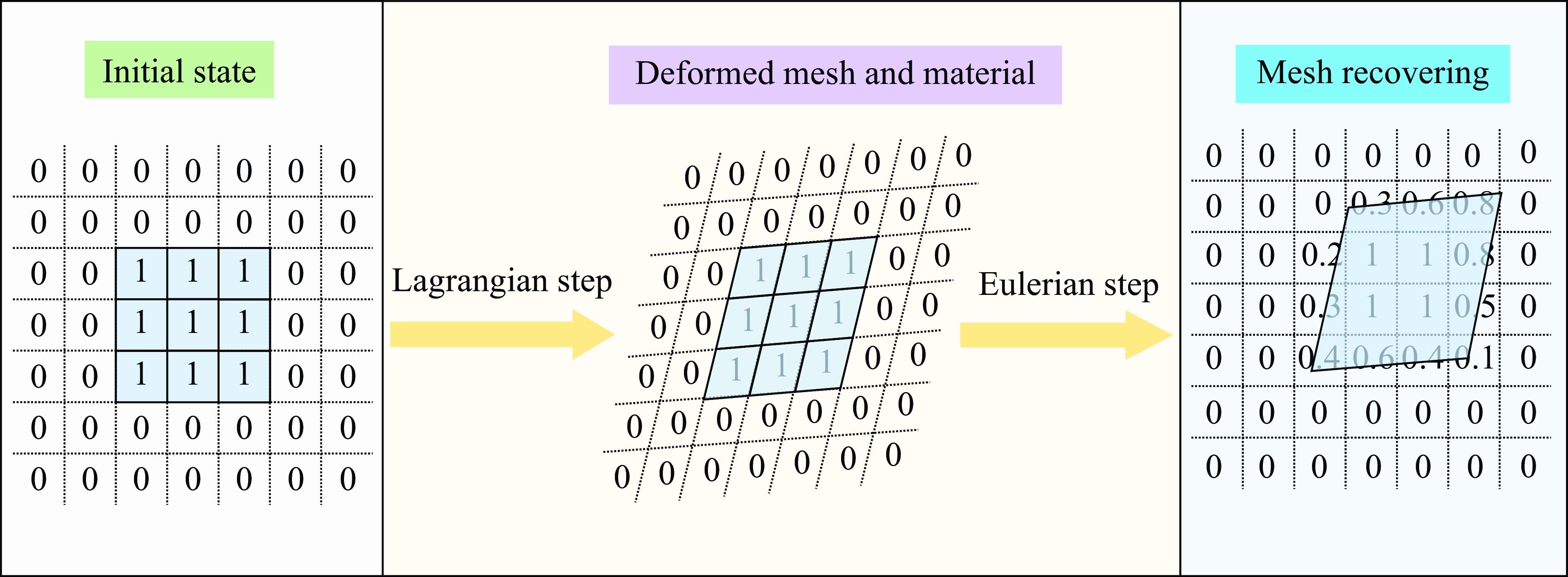
Figure 2. Schematic diagram of the calculation process of the EFEM. The light blue in the grid represents the fluid material, and the numbers represent the volume fraction.
2.2.1. Lagrangian phase
At this stage, the convective terms are eliminated from the governing equation (2.1) and the fluid adheres to the Lagrangian perspective. Meanwhile, we couple the fluid material and the mesh, concentrating merely on the variations of the fluid system within each mesh. Here, taking the momentum equation as an example, when integrated within the mesh, the following form can be obtained:
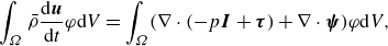 \begin{equation} \int _\Omega \bar \rho \frac {{\rm d} \boldsymbol{u} }{{\rm d}t} \varphi {\rm d}V = \int _\Omega ({ \nabla \cdot (-p \boldsymbol {I}+\boldsymbol{\tau }) + \nabla \cdot \boldsymbol{\psi }} )\varphi {\rm d}V, \end{equation}
where $\varphi$
is the weight function obtained from the mesh shape, and
$\varphi$
is the weight function obtained from the mesh shape, and $\bar \rho = \sum {\alpha \rho }$
is the mixed density. Herein, let us denote
$\bar \rho = \sum {\alpha \rho }$
is the mixed density. Herein, let us denote $\boldsymbol{S}_{\boldsymbol{pvs}} = -p \boldsymbol {I}+ \boldsymbol{\tau } + \boldsymbol{\psi }$
to represent the pressure, viscosity and surface tension terms in the momentum equation. Through partial integration and Gauss transformation, (2.8) can be represented as follows:
$\boldsymbol{S}_{\boldsymbol{pvs}} = -p \boldsymbol {I}+ \boldsymbol{\tau } + \boldsymbol{\psi }$
to represent the pressure, viscosity and surface tension terms in the momentum equation. Through partial integration and Gauss transformation, (2.8) can be represented as follows:
 \begin{equation} \int _\Omega \bar \rho \varphi {\rm d}V \frac {{\rm d} \boldsymbol{u} }{{\rm d}t} +\int _\Omega \varphi \frac {{\rm d} \bar \rho }{{\rm d}t} {\rm d}V \boldsymbol{u} = \int _\Omega {\varphi \boldsymbol{S}_{\boldsymbol{pvs}} \cdot \boldsymbol{n} } {\rm d}\Gamma -\int _\Omega \boldsymbol{S}_{\boldsymbol{pvs}} \nabla \varphi {\rm d}V, \end{equation}
where $\Gamma$
is the boundary of the computational domain
$\Gamma$
is the boundary of the computational domain $\Omega$
,
$\Omega$
, $\boldsymbol{n}$
is the normalised outer normal vector of the boundary. Since the mass of the fluid within the mesh remains invariant, the value of the second term on the right side of (2.9) is zero. Based on the above equations, the node acceleration
$\boldsymbol{n}$
is the normalised outer normal vector of the boundary. Since the mass of the fluid within the mesh remains invariant, the value of the second term on the right side of (2.9) is zero. Based on the above equations, the node acceleration ${{\rm d} \boldsymbol{u} }/{{\rm d}t}$
at the current time can be computed according to the laws of motion, and then the node velocities and displacements can be derived explicitly. Here, the time increment also needs to satisfy the Courant–Friedrichs–Lewy (CFL) condition:
${{\rm d} \boldsymbol{u} }/{{\rm d}t}$
at the current time can be computed according to the laws of motion, and then the node velocities and displacements can be derived explicitly. Here, the time increment also needs to satisfy the Courant–Friedrichs–Lewy (CFL) condition:
 \begin{equation} \Delta t = \lambda {\left ( {\dfrac {{\Delta l}}{{c + \left | \boldsymbol u \right |}}} \right )^{\textit {min} }}, \end{equation}
while $\Delta l$
represents the minimum side length of the mesh, while
$\Delta l$
represents the minimum side length of the mesh, while $\lambda$
denotes the Courant number, set to
$\lambda$
denotes the Courant number, set to $\lambda = 0.2$
in our numerical model to ensure calculation stability. Similarly, the energy equations can be computed during the Lagrangian phase.
$\lambda = 0.2$
in our numerical model to ensure calculation stability. Similarly, the energy equations can be computed during the Lagrangian phase.
2.2.2. Eulerian phase
In the Eulerian phase, the mesh is redrawn based on the original shape and position. To obtain variable values within the new mesh, data exchange between neighbouring meshes is necessary. The Eulerian phase solves the governing equations containing the convective terms, and for the volume fraction
 \begin{equation} \dfrac {{\partial \alpha _k }}{{\partial t}} + \boldsymbol{u} \cdot \nabla \alpha _k = 0. \end{equation}
Solving the equations in the Eulerian phase facilitates the transport of fluid material between adjacent meshes. Pure phase elements utilise a monotone upwind scheme for conservation laws (MUSCL) (Benson Reference Benson1992) for transport, whereas mixed elements are modelled using a quadratic polynomial of volume fraction:
 \begin{equation} \alpha (r,z) = \boldsymbol{\xi } \cdot \boldsymbol{X}, \end{equation}
where $\boldsymbol{\xi }=[\xi _1,\xi _2,\xi _3,\xi _4,\xi _5,\xi _6]$
,
$\boldsymbol{\xi }=[\xi _1,\xi _2,\xi _3,\xi _4,\xi _5,\xi _6]$
, $\boldsymbol{X}=[r^2,z^2,rz,r,z,1]^{\textrm T}$
. Utilising the least-squares technique based on the values of surrounding neighbouring meshes, coefficients
$\boldsymbol{X}=[r^2,z^2,rz,r,z,1]^{\textrm T}$
. Utilising the least-squares technique based on the values of surrounding neighbouring meshes, coefficients $\boldsymbol{\xi }$
can be derived, thereby obtaining the boundary values of the meshes necessary for calculating the transport volume. Furthermore, a half-index shift (HIS) algorithm (Benson Reference Benson2008) is introduced for momentum handling. Upon completion of the Eulerian phase, all variables within the meshes undergo updating, allowing the calculation to proceed into the subsequent time step.
$\boldsymbol{\xi }$
can be derived, thereby obtaining the boundary values of the meshes necessary for calculating the transport volume. Furthermore, a half-index shift (HIS) algorithm (Benson Reference Benson2008) is introduced for momentum handling. Upon completion of the Eulerian phase, all variables within the meshes undergo updating, allowing the calculation to proceed into the subsequent time step.
2.2.3. Boundary conditions
In the EFEM model, the pressure boundary conditions are implemented through the first integration at the right side of (2.9). The upper boundary of the calculation domain is a rigid wall, and the no-slip boundary ( $\boldsymbol u=\boldsymbol 0$
) is applied. In order to minimise the impact of boundaries on bubble pulsation, a non-reflecting boundary was employed. The implementation of non-reflecting boundary conditions is achieved by introducing a transient dynamic pressure
$\boldsymbol u=\boldsymbol 0$
) is applied. In order to minimise the impact of boundaries on bubble pulsation, a non-reflecting boundary was employed. The implementation of non-reflecting boundary conditions is achieved by introducing a transient dynamic pressure $p_d$
at the computational domain boundaries. This dynamic pressure is incorporated into the total pressure
$p_d$
at the computational domain boundaries. This dynamic pressure is incorporated into the total pressure $p$
via superposition. When the computational domain is sufficiently large, the boundary lies in the far field region of bubble dynamics, and the transient dynamic pressure
$p$
via superposition. When the computational domain is sufficiently large, the boundary lies in the far field region of bubble dynamics, and the transient dynamic pressure $p_d$
fulfils the linear acoustic pressure assumption. Consequently, the transient dynamic pressure
$p_d$
fulfils the linear acoustic pressure assumption. Consequently, the transient dynamic pressure $p_d$
satisfies the second-order early-time approximation (
$p_d$
satisfies the second-order early-time approximation ( $\text{ETA}_2$
) equation (Felippa Reference Felippa1980; Liu et al. Reference Liu, Yao, Liu and Yu2018b
). The equation takes the following form:
$\text{ETA}_2$
) equation (Felippa Reference Felippa1980; Liu et al. Reference Liu, Yao, Liu and Yu2018b
). The equation takes the following form:
 \begin{equation} {p_d} + \eta c\int {{p_d}{\rm d}t = \rho c \boldsymbol{u} \cdot \boldsymbol{\omega }}, \end{equation}
where $\eta$
is the wavefront surface curvature and
$\eta$
is the wavefront surface curvature and $\boldsymbol{\omega }$
is the pressure wave propagation direction. Additionally, the viscous effect within the boundary is accounted for in the viscous normal stress
$\boldsymbol{\omega }$
is the pressure wave propagation direction. Additionally, the viscous effect within the boundary is accounted for in the viscous normal stress $\boldsymbol{\tau }_{{ii}}$
in (2.9).
$\boldsymbol{\tau }_{{ii}}$
in (2.9).
2.3. Dimensionless parameters
In order to streamline the investigation of bubble dynamics, a dimensionless variable system was employed. Three physical quantities, namely the average maximum radius of bubbles $R_{max }$
, the density of water
$R_{max }$
, the density of water $\rho _{{w}}=998 \, \text{kg m}^{-3}$
and atmospheric pressure
$\rho _{{w}}=998 \, \text{kg m}^{-3}$
and atmospheric pressure $P_{{atm}} = 101\,325\,{\textrm {Pa}}$
, were chosen as the basic parameters. Correspondingly, velocity, time and acceleration are symbolised by
$P_{{atm}} = 101\,325\,{\textrm {Pa}}$
, were chosen as the basic parameters. Correspondingly, velocity, time and acceleration are symbolised by $\sqrt {{{\mathop {P}\nolimits } _{{atm}}}/{\rho _{{w}}}}$
,
$\sqrt {{{\mathop {P}\nolimits } _{{atm}}}/{\rho _{{w}}}}$
, ${R_{max }}\sqrt {{\rho _{{w}}} / {{\mathop {P}\nolimits } _{{atm}}}}$
and
${R_{max }}\sqrt {{\rho _{{w}}} / {{\mathop {P}\nolimits } _{{atm}}}}$
and ${{\mathop {P}\nolimits } _{{atm}}}/ ( {{R_{max }}{\rho _{{w}}}} )$
, respectively. The viscosity of the silicone oil is denoted as
${{\mathop {P}\nolimits } _{{atm}}}/ ( {{R_{max }}{\rho _{{w}}}} )$
, respectively. The viscosity of the silicone oil is denoted as $\mu ^* = \mu /({R_{max }}\sqrt {{\rho _{{w}}}{{\mathop {P}\nolimits } _{{atm}}}})$
. The bubble–wall distance and initial oil-layer thickness are denoted by dimensionless distances
$\mu ^* = \mu /({R_{max }}\sqrt {{\rho _{{w}}}{{\mathop {P}\nolimits } _{{atm}}}})$
. The bubble–wall distance and initial oil-layer thickness are denoted by dimensionless distances $\gamma = d/{R_{max }},\delta = h/{R_{max }}$
, respectively. In this paper, except for the model validation section, all variables are dimensionless. A superscript symbol ‘*’ is also used to represent dimensionless variables.
$\gamma = d/{R_{max }},\delta = h/{R_{max }}$
, respectively. In this paper, except for the model validation section, all variables are dimensionless. A superscript symbol ‘*’ is also used to represent dimensionless variables.
2.4. Validation and mesh independence test
To validate the numerical model, laser-induced cavitation bubble experiments were conducted. The laser induced cavitation bubbles in the water medium, and high-speed cameras captured the evolution of bubbles and oil layers at a speed of 180 000 frames per second. A $0.5\, {\textrm {mm}}$
thick acrylic ring filled with silicone oil of
$0.5\, {\textrm {mm}}$
thick acrylic ring filled with silicone oil of $1000cSt$
viscosity was employed as the viscous layer. The laser-induced cavitation bubble formed in proximity to the oil layer, exhibiting a maximum bubble radius of
$1000cSt$
viscosity was employed as the viscous layer. The laser-induced cavitation bubble formed in proximity to the oil layer, exhibiting a maximum bubble radius of $R_{max }=1.08\, {\textrm {mm}}$
and an initial distance of
$R_{max }=1.08\, {\textrm {mm}}$
and an initial distance of $1.06\, {\textrm {mm}}$
(that is,
$1.06\, {\textrm {mm}}$
(that is, $\gamma =0.981$
) from the rigid wall. The thickness of the viscous silicone-oil layer is
$\gamma =0.981$
) from the rigid wall. The thickness of the viscous silicone-oil layer is $h = 0.5\, {\textrm {mm}}$
(that is,
$h = 0.5\, {\textrm {mm}}$
(that is, $\delta = 0.463$
). The numerical model features a calculation domain size of
$\delta = 0.463$
). The numerical model features a calculation domain size of $12\, {\textrm {mm}} \times 8\, {\textrm {mm}}$
. Non-reflecting boundaries were implemented on the lateral sides. The initial bubble radius was defined as
$12\, {\textrm {mm}} \times 8\, {\textrm {mm}}$
. Non-reflecting boundaries were implemented on the lateral sides. The initial bubble radius was defined as $R_0=0.1R_{max }$
, with the surrounding fluid pressure set at atmospheric pressure, while the initial bubble pressure was adjusted to match the experimental conditions, ultimately determining a pressure of
$R_0=0.1R_{max }$
, with the surrounding fluid pressure set at atmospheric pressure, while the initial bubble pressure was adjusted to match the experimental conditions, ultimately determining a pressure of $P_0=57\, {\textrm {MPa}}$
. Figure 3 demonstrates the contrast between the numerical model and the experimental data at the same dimensionless time, with the red contours representing the interface of the numerical bubble.
$P_0=57\, {\textrm {MPa}}$
. Figure 3 demonstrates the contrast between the numerical model and the experimental data at the same dimensionless time, with the red contours representing the interface of the numerical bubble.
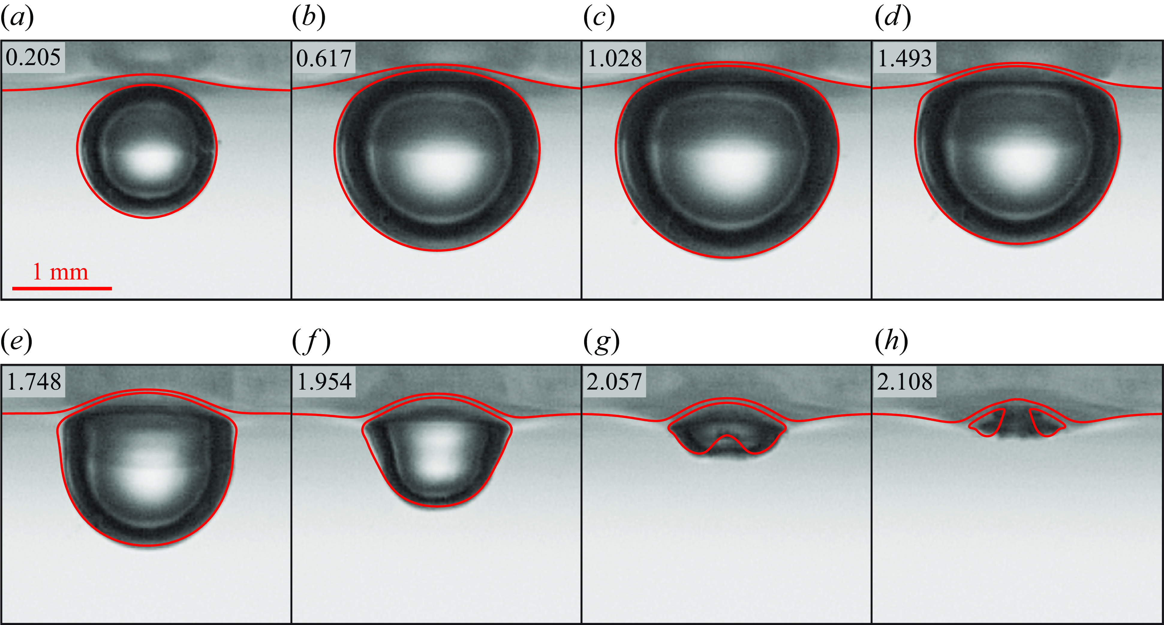
Figure 3. Comparison between EFEM bubble dynamics model and experimental results ( $1000cSt$
silicone oil) at
$1000cSt$
silicone oil) at $t^*=0.205,0.617,1.028,1.493,1.748,1.954,2.057,2.108$
,
$t^*=0.205,0.617,1.028,1.493,1.748,1.954,2.057,2.108$
, $\delta =0.463$
,
$\delta =0.463$
, $\gamma =0.981$
. The upper boundary of the window is a rigid wall with a layer of silicone oil attached below. The images represent the experiments, and the red contours indicate the numerical results.
$\gamma =0.981$
. The upper boundary of the window is a rigid wall with a layer of silicone oil attached below. The images represent the experiments, and the red contours indicate the numerical results.
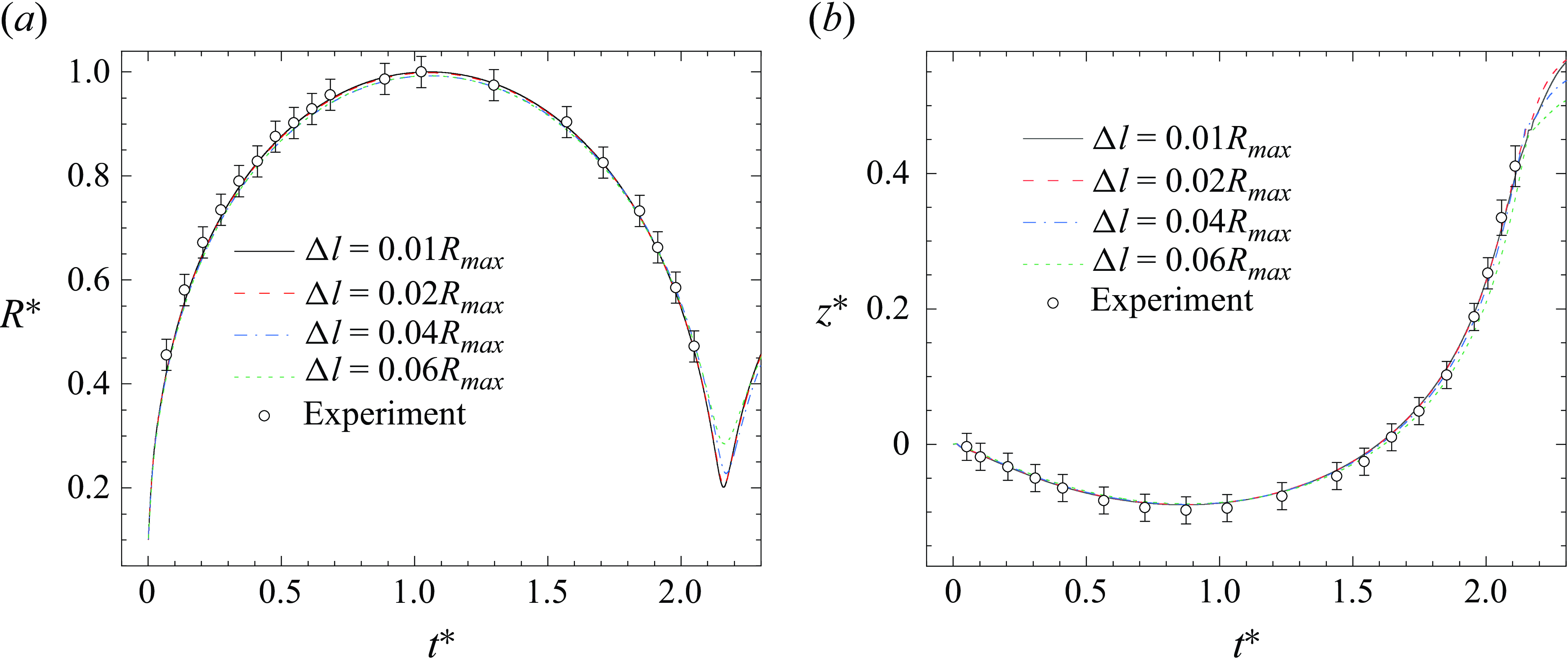
Figure 4. Evolution of (a) the bubble radius R and (b) the bubble mass centre at mesh sizes 0.01 $R_{max }$
, 0.02
$R_{max }$
, 0.02 $R_{max }$
, 0.04
$R_{max }$
, 0.04 $R_{max }$
, 0.06
$R_{max }$
, 0.06 $R_{max }$
and experiments. The circular error bars illustrate the experimental results, with an uncertainty of one pixel.
$R_{max }$
and experiments. The circular error bars illustrate the experimental results, with an uncertainty of one pixel.
Figure 3(a–c) illustrates the process of bubble expansion, while panels (d–h) delineate the process of bubble collapse. The upper portion of the bubble expands slowly as it is hindered by the oil layer. During the collapse phase, it is pulled by the oil layer, leading to a slow contraction. The asymmetrical expansion and collapse give rise to a bubble jet directed towards the silicone-oil layer. The EFEM model precisely calculates the contour of the bubble and the form of the silicone-oil interface.
Moreover, the evolution of the bubble radius and the bubble mass centre was compared between the experimental and numerical results, shown in figure 4. A mesh independence test has also been carried out here, with numerical models using mesh sizes of 0.01 $R_{max }$
, 0.02
$R_{max }$
, 0.02 $R_{max }$
, 0.04
$R_{max }$
, 0.04 $R_{max }$
and 0.06
$R_{max }$
and 0.06 $R_{max }$
, respectively. It can be observed from figure 4(a) that the bubble radius in the expansion stage of the experiment is slightly larger than that of the numerical results. This is mainly because the initial expansion of the nucleated bubble is intense, and the radius increases rapidly. In contrast, the initial pressure in the numerical model is lower, resulting in a relatively slow expansion. Nevertheless, both the numerical and experimental results can reach the same maximum radius, and the disparity between them lies within the measurement error range (one pixel length). With the maximum bubble radius serving as the reference quantity, the relative errors of the results from different meshes are 1.69 %, 0.58 % and 0.17 %, respectively. This implies that as the mesh size decreases, the computational results of the numerical model converge. The migration of the bubble mass centre in the numerical model also shows a good agreement with the experimental results (figure 4
b), which suffices to demonstrate the accuracy of the numerical model. In the present investigation, the minimum mesh size is set at
$R_{max }$
, respectively. It can be observed from figure 4(a) that the bubble radius in the expansion stage of the experiment is slightly larger than that of the numerical results. This is mainly because the initial expansion of the nucleated bubble is intense, and the radius increases rapidly. In contrast, the initial pressure in the numerical model is lower, resulting in a relatively slow expansion. Nevertheless, both the numerical and experimental results can reach the same maximum radius, and the disparity between them lies within the measurement error range (one pixel length). With the maximum bubble radius serving as the reference quantity, the relative errors of the results from different meshes are 1.69 %, 0.58 % and 0.17 %, respectively. This implies that as the mesh size decreases, the computational results of the numerical model converge. The migration of the bubble mass centre in the numerical model also shows a good agreement with the experimental results (figure 4
b), which suffices to demonstrate the accuracy of the numerical model. In the present investigation, the minimum mesh size is set at $\Delta l=0.01R_{max }$
, which can capture flow details more accurately. Furthermore, it is worth clarifying that, due to the constraints of the equipment, the shock wave at the wall surface could not be measured. Hence, the bubble shock wave has not been verified in this paper. The shock-wave load is associated with the initial parameters of the bubble, the distance and the environment. Based on the initial conditions adopted in this paper, the measurement of the wall shock wave is for regularity research rather than representing the actual wall load value in practical scenarios.
$\Delta l=0.01R_{max }$
, which can capture flow details more accurately. Furthermore, it is worth clarifying that, due to the constraints of the equipment, the shock wave at the wall surface could not be measured. Hence, the bubble shock wave has not been verified in this paper. The shock-wave load is associated with the initial parameters of the bubble, the distance and the environment. Based on the initial conditions adopted in this paper, the measurement of the wall shock wave is for regularity research rather than representing the actual wall load value in practical scenarios.
3. Results and discussion
In this study, experimental results and numerical models are employed to analyse the dimensionless bubble–wall distance ( $\gamma =0.4{-}2.0$
). The thickness of the silicone-oil layer is consistently maintained below the bubble–wall distance to ensure the formation of bubbles in water. The viscosity
$\gamma =0.4{-}2.0$
). The thickness of the silicone-oil layer is consistently maintained below the bubble–wall distance to ensure the formation of bubbles in water. The viscosity $\mu ^*$
of the silicone oil ranges from 0.001 to 1.3. In the current numerical model, the computational domain size is
$\mu ^*$
of the silicone oil ranges from 0.001 to 1.3. In the current numerical model, the computational domain size is $6R_{max } \times 8R_{max }$
, the initial bubble radius is set to
$6R_{max } \times 8R_{max }$
, the initial bubble radius is set to $R_0=0.101R_{max }$
, and the initial pressure is
$R_0=0.101R_{max }$
, and the initial pressure is $P_0=55\, {\textrm {MPa}}$
.
$P_0=55\, {\textrm {MPa}}$
.
3.1. The dynamics of cavitation bubbles in the experiment
In this section, we experimentally investigate and compare the bubble pulsation and oil-layer movement across three distinct scenarios. In the experiment, the viscosity range of silicone oil was set between 100 and 1000 $cSt$
. Consequently, under varying conditions, differences in bubble size led to variations in the corresponding dimensionless viscosity values. It is important to note that this study compares scenarios with identical dimensionless parameters; therefore, bubble size does not significantly influence the results. For each condition, images exhibiting similar phenomena or captured at corresponding time points were extracted for comparative analysis. The maximum radius of the bubbles observed in the experiment was approximately 1.08 mm. We analyse the influence of silicone-oil-layer viscosity, silicone-oil-layer thickness, and bubble–wall distance on the bubble–wall–oil-layer system.
$cSt$
. Consequently, under varying conditions, differences in bubble size led to variations in the corresponding dimensionless viscosity values. It is important to note that this study compares scenarios with identical dimensionless parameters; therefore, bubble size does not significantly influence the results. For each condition, images exhibiting similar phenomena or captured at corresponding time points were extracted for comparative analysis. The maximum radius of the bubbles observed in the experiment was approximately 1.08 mm. We analyse the influence of silicone-oil-layer viscosity, silicone-oil-layer thickness, and bubble–wall distance on the bubble–wall–oil-layer system.
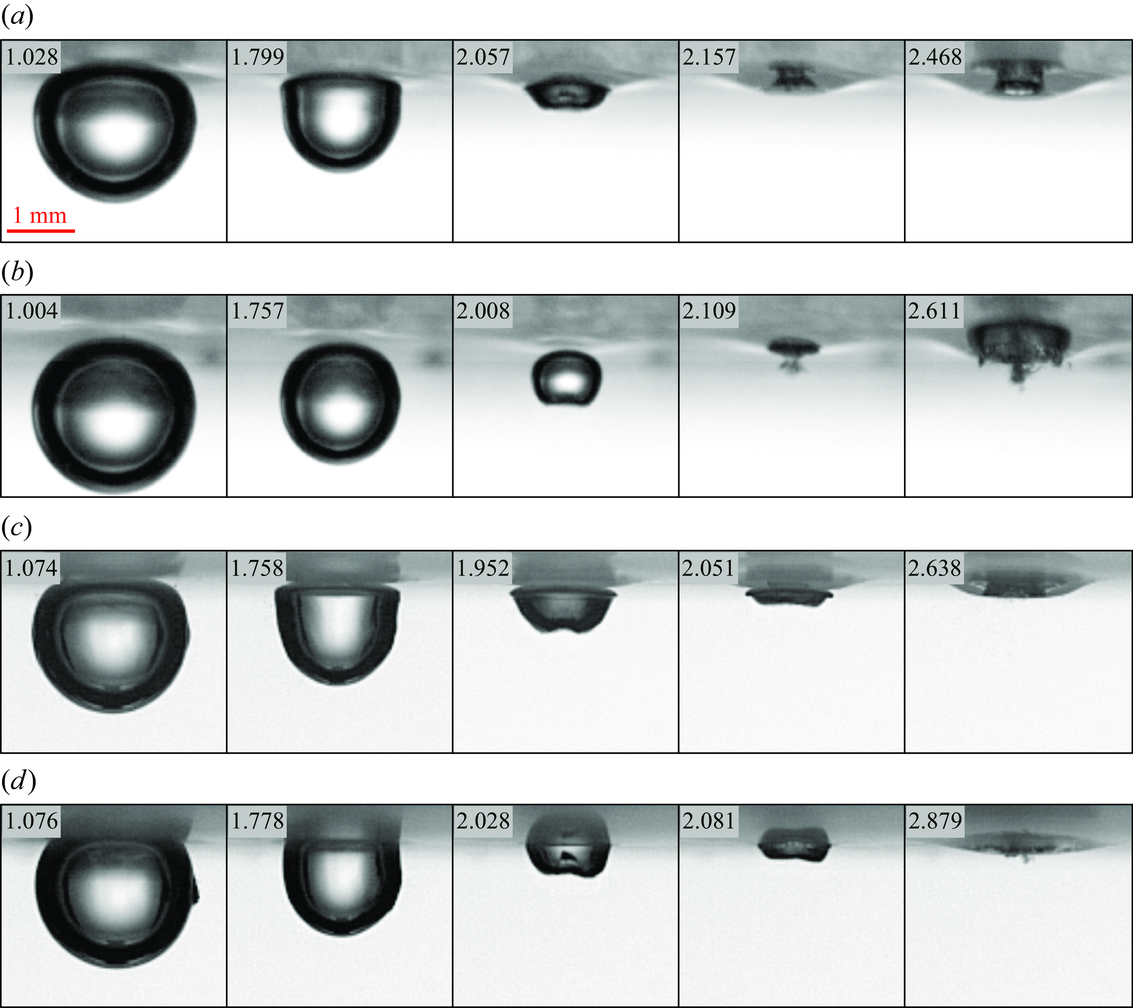
Figure 5. Evolution of bubbles and silicone-oil interface at (a) $\delta = 0.463$
,
$\delta = 0.463$
, $\gamma =0.981$
,
$\gamma =0.981$
, $\mu ^*=0.089$
; (b)
$\mu ^*=0.089$
; (b) $\delta = 0.47$
,
$\delta = 0.47$
, $\gamma =1.374$
,
$\gamma =1.374$
, $\mu ^*=0.087$
; (c)
$\mu ^*=0.087$
; (c) $\delta = 0.356$
,
$\delta = 0.356$
, $\gamma =0.986$
,
$\gamma =0.986$
, $\mu ^*=0.088$
; (d)
$\mu ^*=0.088$
; (d) $\delta = 0.454$
,
$\delta = 0.454$
, $\gamma =0.981$
,
$\gamma =0.981$
, $\mu ^*=0.0089$
.
$\mu ^*=0.0089$
.
In figure 5, four distinct experiments are presented. With figure 5(a) as the reference, panels (b–d) represent different distance parameters, thicknesses of the viscous oil layer and viscosities, respectively. First, the influence of the bubble–wall distance on the system was investigated. As illustrated in figures 5(a) and 5(b), the bubble collapsed near a silicone-oil layer with a viscosity of 1000 $cSt$
(
$cSt$
( $\mu ^*=0.089$
). The thicknesses of the oil layers were
$\mu ^*=0.089$
). The thicknesses of the oil layers were $\delta=0.463$
and 0.47, corresponding to stand-off distances
$\delta=0.463$
and 0.47, corresponding to stand-off distances $\gamma=0.981$
and 1.374, respectively. During the initial collapse phase, bubbles at both distances did not penetrate into the silicone oil. However, bubbles closer to the wall made contact with the oil layer prior to collapse, leading to a pronounced ‘dragged’ effect from the oil layer on the upper surface. This resulted in a high-curvature edge, causing the bubble to exhibit a flattened top and rounded bottom shape. Conversely, the more distant bubble maintained highly spherical form during collapse, similar to that observed near a pure solid wall. At the moment when the water jet within the bubble was about to penetrate the opposite side (
$\gamma=0.981$
and 1.374, respectively. During the initial collapse phase, bubbles at both distances did not penetrate into the silicone oil. However, bubbles closer to the wall made contact with the oil layer prior to collapse, leading to a pronounced ‘dragged’ effect from the oil layer on the upper surface. This resulted in a high-curvature edge, causing the bubble to exhibit a flattened top and rounded bottom shape. Conversely, the more distant bubble maintained highly spherical form during collapse, similar to that observed near a pure solid wall. At the moment when the water jet within the bubble was about to penetrate the opposite side ( $t^*=2.09$
), approximately half the volume of the bubble at
$t^*=2.09$
), approximately half the volume of the bubble at $\gamma=0.981$
had entered the oil layer, while the entire bubble at
$\gamma=0.981$
had entered the oil layer, while the entire bubble at $\gamma=1.374$
remained in water. Following the occurrence of the jet, the bubble rapidly migrated towards the oil layer. In figure 5(a), the bubble became completely immersed in the silicone oil and subsequently expanded again within it. For the more distant bubble (
$\gamma=1.374$
remained in water. Following the occurrence of the jet, the bubble rapidly migrated towards the oil layer. In figure 5(a), the bubble became completely immersed in the silicone oil and subsequently expanded again within it. For the more distant bubble ( $\gamma=1.374$
), only partial entry into the silicone oil was observed. Although it was not feasible to measure the bubble volume after entering the reservoir, based on the shorter bubble period (the time difference between the fifth and fourth images equating to half a period), it can be inferred that the rebound volume of the bubble in the oil is less than that in water, consistent with expectations due to the viscous resistance. It can also be deduced that the viscous layer must impede subsequent bubble collapse, thereby reducing the impact load of the cavitation bubble on the wall.
$\gamma=1.374$
), only partial entry into the silicone oil was observed. Although it was not feasible to measure the bubble volume after entering the reservoir, based on the shorter bubble period (the time difference between the fifth and fourth images equating to half a period), it can be inferred that the rebound volume of the bubble in the oil is less than that in water, consistent with expectations due to the viscous resistance. It can also be deduced that the viscous layer must impede subsequent bubble collapse, thereby reducing the impact load of the cavitation bubble on the wall.
Subsequently, observe figure 5(c), in contrast to figure 5(a), where a thinner viscous oil layer adheres to the wall surface. At the moment of maximum radius, the bubble shapes in both cases exhibit a strong degree of similarity, as the bubbles are both retarded by the viscous layer and the wall. On closer inspection, however, it can be discerned that the upper part of the bubble in figure 5(c) is flatter. In addition to the fact that the bubble walls are smaller in distance than in figure 5(a), the reduced buffering effect of the thinner viscous oil layer at the bubble boundary is also a contributing factor. The distinction in the shape of the bubble’s top is more pronounced in the image of the second column from the left in figure 5, where the wall effect begins to become prominent. Before the jet penetrates, the bubble in figure 5(c) has a broader lateral scale and concurrently induces a larger water column (composed of water and vapour mixture) in the oil layer, which will exacerbate the jet’s impact on the wall. The reason lies in the fact that a thinner viscous layer has a weaker inhibitory effect on the lateral pulsation of the bubble compared with a thicker viscous layer. Finally, the effect of viscosity is analysed and presented in figure 5(d). The physical viscosity of the oil layer is 100 $cSt$
(
$cSt$
( $\mu ^*= 0.0089$
). At this low viscosity, the influence of the oil layer on the coupled system is relatively weak and the sphericity of the bubble increases. The modification of the bubble shape originates primarily from the rigid wall. By comparing the last image in figures 5(a) and 5(d), the bulge at the oil–water interface due to bubble pulsation within the oil layer is smaller when the viscosity of the oil layer is lower. This is due to the lower viscous resistance to the lateral expansion of the bubble. Besides expanding downward, the bubble can also more readily diffuse along the wall. In the case of high viscosity (figure 5
a), the bubble’s downward expansion is more facile, as the mixture below is water–vapour–oil with lower viscosity, thereby causing a larger interface bulge.
$\mu ^*= 0.0089$
). At this low viscosity, the influence of the oil layer on the coupled system is relatively weak and the sphericity of the bubble increases. The modification of the bubble shape originates primarily from the rigid wall. By comparing the last image in figures 5(a) and 5(d), the bulge at the oil–water interface due to bubble pulsation within the oil layer is smaller when the viscosity of the oil layer is lower. This is due to the lower viscous resistance to the lateral expansion of the bubble. Besides expanding downward, the bubble can also more readily diffuse along the wall. In the case of high viscosity (figure 5
a), the bubble’s downward expansion is more facile, as the mixture below is water–vapour–oil with lower viscosity, thereby causing a larger interface bulge.
3.2. Bubble dynamics with different silicone-oil-layer thicknesses
3.2.1. Effect of viscous oil-layer thickness on bubbles at $\mu ^*=0.0065$

The simulation initially focused on the oil layer with low viscosity $\mu ^*=0.0065$
. Figure 6 depicts the evolution of the bubble near the oil layer with viscosity
$\mu ^*=0.0065$
. Figure 6 depicts the evolution of the bubble near the oil layer with viscosity $\mu ^*=0.0065$
and a thickness of
$\mu ^*=0.0065$
and a thickness of $\delta =1.0$
. Figure 6(a) shows the initial moment that the bubble is filled with high-pressure non-condensable gas. Figure 6(b) demonstrates the refraction and transmission of the pressure wave emitted by the bubble at the oil-water interface, where the transmitted wave is shown as a equivalent shear stress parameter
$\delta =1.0$
. Figure 6(a) shows the initial moment that the bubble is filled with high-pressure non-condensable gas. Figure 6(b) demonstrates the refraction and transmission of the pressure wave emitted by the bubble at the oil-water interface, where the transmitted wave is shown as a equivalent shear stress parameter $ |\boldsymbol{\tau }|=\sqrt {0.5\boldsymbol{\tau } : \boldsymbol{\tau }}$
. Observations indicate that shock waves and reflected waves form spherical shapes, while equivalent shear stress appear non-spherical. This difference arises from the varying sound speeds in silicone oil and water, with both pressure and equivalent shear stress propagating at velocities comparable to sound speed. The sound speeds in this study are determined using (2.5), defined here as
$ |\boldsymbol{\tau }|=\sqrt {0.5\boldsymbol{\tau } : \boldsymbol{\tau }}$
. Observations indicate that shock waves and reflected waves form spherical shapes, while equivalent shear stress appear non-spherical. This difference arises from the varying sound speeds in silicone oil and water, with both pressure and equivalent shear stress propagating at velocities comparable to sound speed. The sound speeds in this study are determined using (2.5), defined here as $c_{{water}}=1540\, \rm kg\, \rm s^{-1}$
and
$c_{{water}}=1540\, \rm kg\, \rm s^{-1}$
and $c_{{oil}}=978\, \rm kg\,s^{-1}$
. At
$c_{{oil}}=978\, \rm kg\,s^{-1}$
. At $t^*=1.002$
, the bubble expands to its maximum radius. Due to the no-slip boundary at the rigid wall, a thin region of high shear stress forms near the wall surface shown in figure 6(d). Zeng et al. (Reference Zeng, Gonzalez-Avila, Dijkink, Koukouvinis, Gavaises and Ohl2018, Reference Zeng, An and Ohl2022) conducted detailed simulations of the wall shear stress, which has significant applications in bubble cleaning. In figure 6(f), the bubble collapses, creating jets directed towards the silicone-oil layer and rigid wall. The jet penetrates the bubble, entering the oil layer by
$t^*=1.002$
, the bubble expands to its maximum radius. Due to the no-slip boundary at the rigid wall, a thin region of high shear stress forms near the wall surface shown in figure 6(d). Zeng et al. (Reference Zeng, Gonzalez-Avila, Dijkink, Koukouvinis, Gavaises and Ohl2018, Reference Zeng, An and Ohl2022) conducted detailed simulations of the wall shear stress, which has significant applications in bubble cleaning. In figure 6(f), the bubble collapses, creating jets directed towards the silicone-oil layer and rigid wall. The jet penetrates the bubble, entering the oil layer by $t^*=2.123$
, at which point the bubble is completely immersed in the oil layer. Figure 6(h) reveals the bubble jet’s impact on the rigid wall, generating a region characterised by high pressure and shear stress. Guided by the bubble, the gas-water mixture infiltrates the oil layer, a phenomenon explored in detail by Ohl et al. (Reference Ohl, Reese and Ohl2024), who investigated various manifestations of the gas-water mixture within the oil layer.
$t^*=2.123$
, at which point the bubble is completely immersed in the oil layer. Figure 6(h) reveals the bubble jet’s impact on the rigid wall, generating a region characterised by high pressure and shear stress. Guided by the bubble, the gas-water mixture infiltrates the oil layer, a phenomenon explored in detail by Ohl et al. (Reference Ohl, Reese and Ohl2024), who investigated various manifestations of the gas-water mixture within the oil layer.
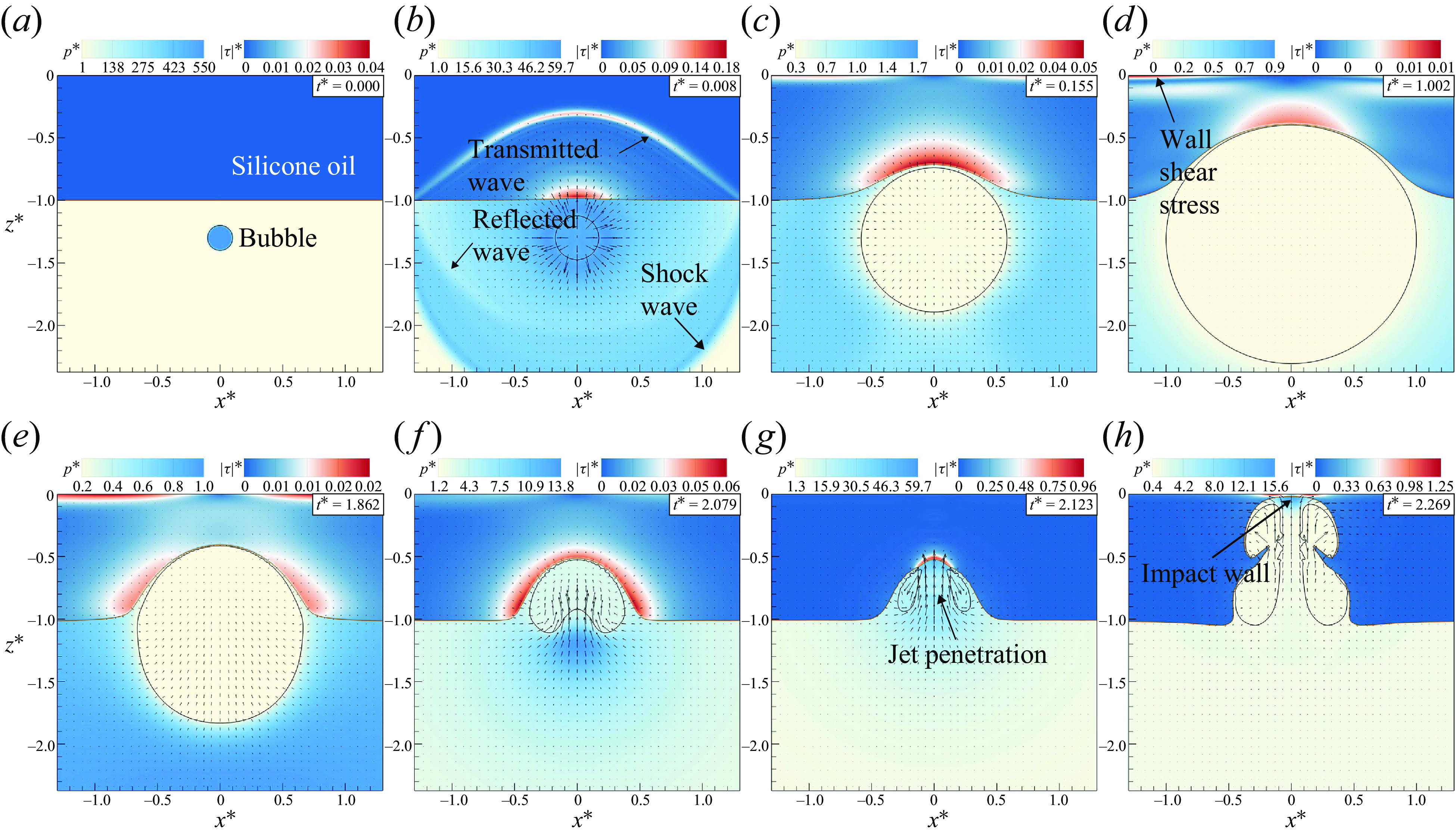
Figure 6. The evolution process of cavitation bubbles near the wall-attached oil layer at $t^*=0, 0.008,0.155,1.002,1.862,2.079,2.123,2.269$
,
$t^*=0, 0.008,0.155,1.002,1.862,2.079,2.123,2.269$
, $\gamma =1.3$
,
$\gamma =1.3$
, $\delta =1.0$
,
$\delta =1.0$
, $\mu ^*=0.0065$
. The black line represents the bubble interface. The brown line represents the oil–water interface, and the arrows indicate velocity vectors. The
$\mu ^*=0.0065$
. The black line represents the bubble interface. The brown line represents the oil–water interface, and the arrows indicate velocity vectors. The $x^*$
represents the radial coordinate. The lower part of each contour plot represents pressure, while the upper part of each contour plot displays the equivalent shear stress.
$x^*$
represents the radial coordinate. The lower part of each contour plot represents pressure, while the upper part of each contour plot displays the equivalent shear stress.
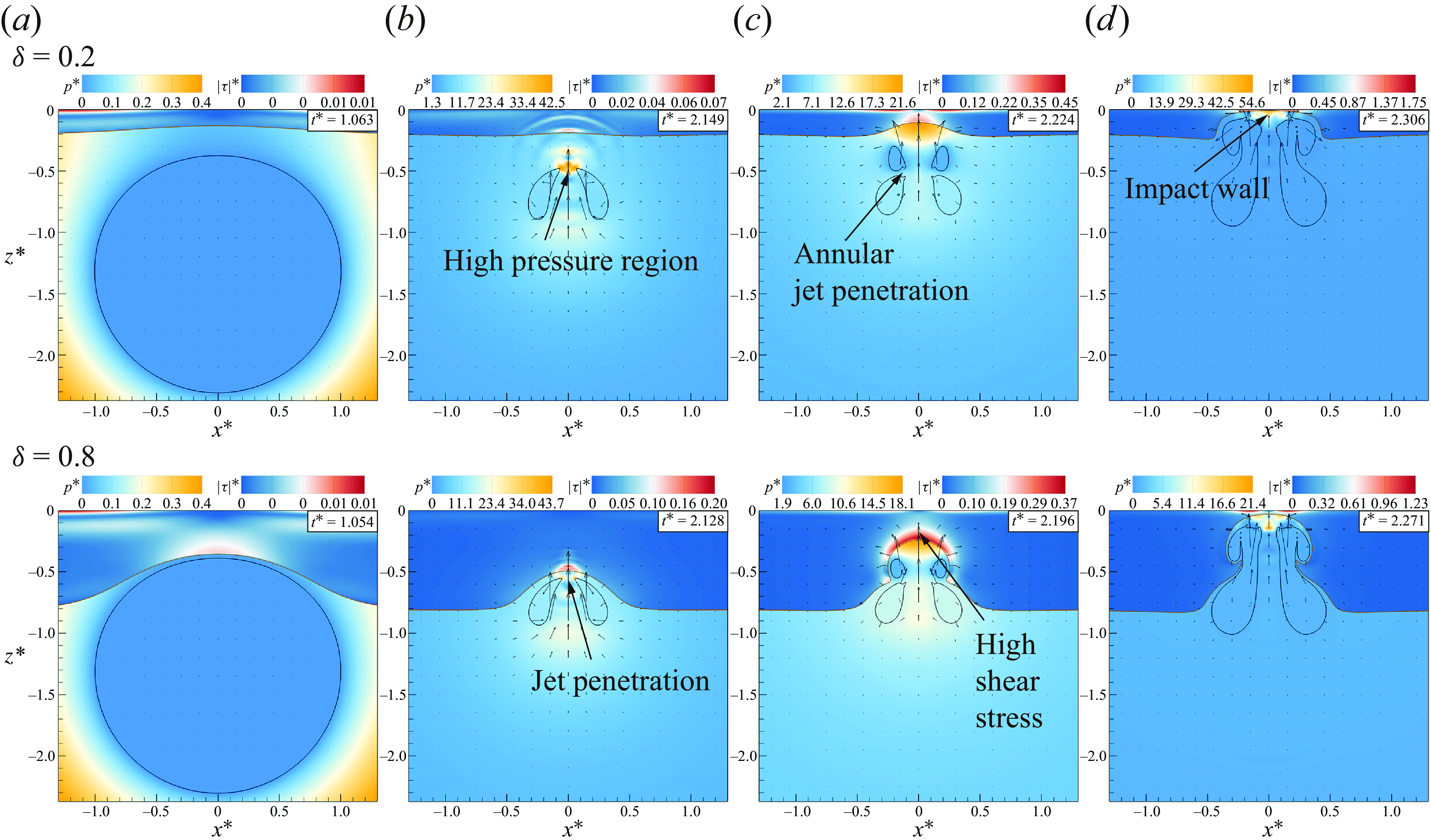
Figure 7. Evolution of bubbles and silicone-oil interface at oil-layer thicknesses $\delta = 0.2$
and
$\delta = 0.2$
and $0.8$
,
$0.8$
, $\gamma =1.3$
,
$\gamma =1.3$
, $\mu ^*=0.0065$
.
$\mu ^*=0.0065$
.
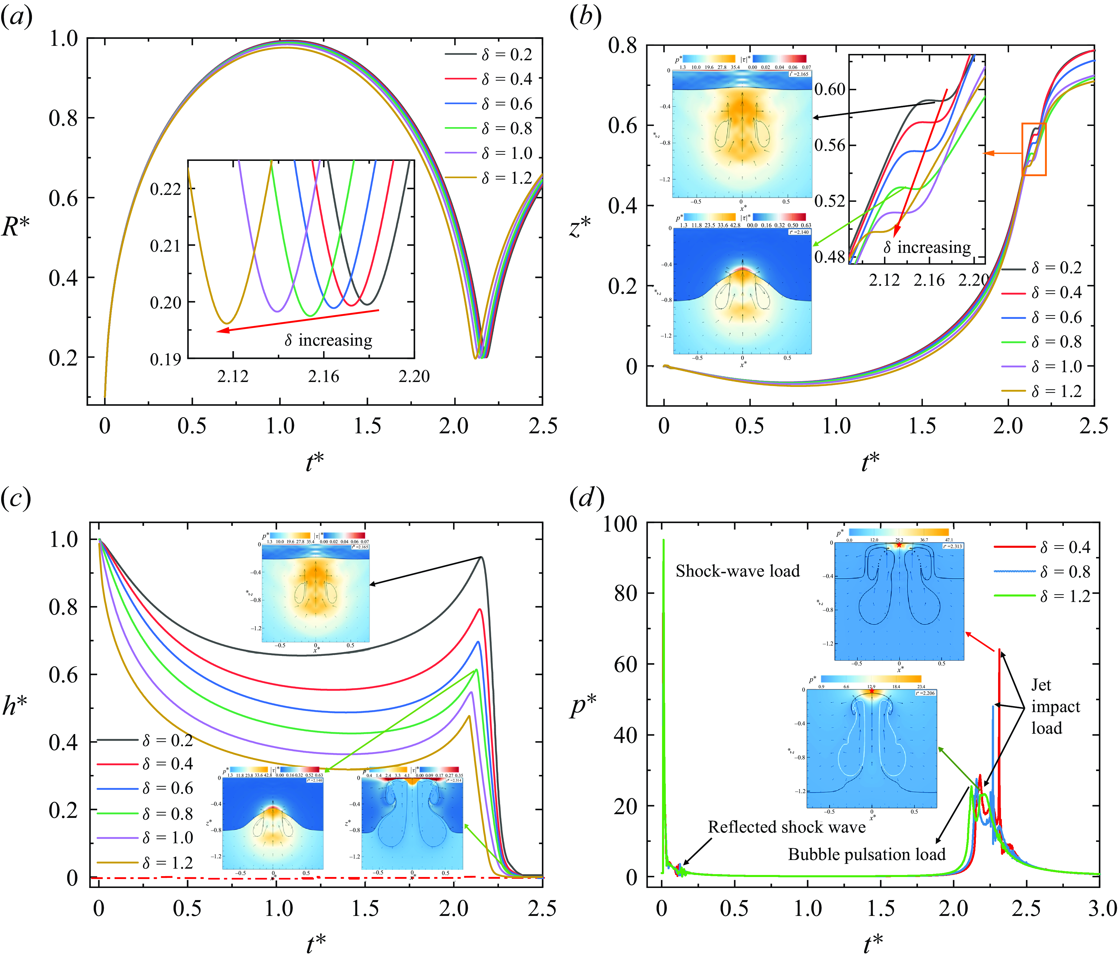
Figure 8. Time evolution for (a) bubble radius, (b) centre of mass position, (c) oil-layer thickness, (d) wall centre pressure at oil-layer thickness $\delta =$
0.2–1.2, stand-off distance
$\delta =$
0.2–1.2, stand-off distance $\gamma =1.3$
, viscosity
$\gamma =1.3$
, viscosity $\mu ^*=0.0065$
.
$\mu ^*=0.0065$
.
Figure 7 illustrates the collapse of the bubble and variations in the oil–water interface for oil-layer thicknesses $\delta =0.2$
and 0.8. The motion of the bubble is quite similar, with the moments of maximum expansion (figure 7
a) and jet penetration (figure 7
b) being closely matched. Figure 7(c) shows the division of the bubble by the annular jet. Notably, when compared with the thinner oil layer, the volume ratio of the bifurcated annular bubbles significantly increases at
$\delta =0.2$
and 0.8. The motion of the bubble is quite similar, with the moments of maximum expansion (figure 7
a) and jet penetration (figure 7
b) being closely matched. Figure 7(c) shows the division of the bubble by the annular jet. Notably, when compared with the thinner oil layer, the volume ratio of the bifurcated annular bubbles significantly increases at $\delta =0.8$
. This effect arises primarily from the annular jets induced by fluid vortices, whose formation is impeded by the thicker oil layer. The oil layer also attenuates the bubble jet, resulting in a smaller wall impact pressure, as in figure 7(d).
$\delta =0.8$
. This effect arises primarily from the annular jets induced by fluid vortices, whose formation is impeded by the thicker oil layer. The oil layer also attenuates the bubble jet, resulting in a smaller wall impact pressure, as in figure 7(d).
Figure 8 illustrates the temporal evolution of the bubble radius, migration of the mass centre, normalised oil-layer thickness, and the central pressure load on the rigid wall across various oil-layer thicknesses. It is evident from figure 8 that the low viscosity of silicone oil minimally influences bubble dynamics, a notion corroborated by the bubble shape evolution shown in figure 7. Figure 8(a) demonstrates that with increasing oil-layer thickness, bubbles possessing identical initial energy achieve a reduced maximum radius, and the associated bubble oscillation period diminishes, yet the bubble’s minimum collapse radius remains largely unaffected. For oil-layer thicknesses $\delta$
ranging from 0.2 to 1.2, the relative variations in bubble radius are 0.16 %, 0.17 %, 0.27 %, 0.35 % and 0.82 %, respectively, signifying that the oil layer’s influence on the bubble escalates with thickness. Figure 8(b) shows the progression of the bubble’s mass centre migration. Since gravity is neglected, the main contributors to bubble migration are the walls and the ‘attraction’ of the oil layer. Taking the initial spherical centre of the bubble as the origin, the centre of mass of the bubble moves away from the oil layer and the wall during the expansion phase, as the oil layer hinders the bubble motion, causing the bubble to expand more towards the water. Throughout the contraction phase, the centre of mass of the bubble rapidly ascends. Upon jet penetration, the bubble’s mass centre remains nearly unchanged for a brief period. An inset in figure 8(b) highlights this transient pause of the bubble’s mass centre, accompanied by two subfigures illustrating the pressure and equivalent shear stress contour maps at that instant.
$\delta$
ranging from 0.2 to 1.2, the relative variations in bubble radius are 0.16 %, 0.17 %, 0.27 %, 0.35 % and 0.82 %, respectively, signifying that the oil layer’s influence on the bubble escalates with thickness. Figure 8(b) shows the progression of the bubble’s mass centre migration. Since gravity is neglected, the main contributors to bubble migration are the walls and the ‘attraction’ of the oil layer. Taking the initial spherical centre of the bubble as the origin, the centre of mass of the bubble moves away from the oil layer and the wall during the expansion phase, as the oil layer hinders the bubble motion, causing the bubble to expand more towards the water. Throughout the contraction phase, the centre of mass of the bubble rapidly ascends. Upon jet penetration, the bubble’s mass centre remains nearly unchanged for a brief period. An inset in figure 8(b) highlights this transient pause of the bubble’s mass centre, accompanied by two subfigures illustrating the pressure and equivalent shear stress contour maps at that instant.
The thickness of the silicone oil plays a crucial role in investigating the impacts of bubble jets. Figure 8(c) illustrates the evolution of the normalised oil-layer thickness at the symmetry axis, where $h^* = h/{\delta }$
, with the initial thickness set at 1.0, and
$h^* = h/{\delta }$
, with the initial thickness set at 1.0, and $h^* = 0$
indicating the disappearance of the oil layer. Influenced by the upper surface of the bubble, the oil-layer thickness gradually decreases during the bubble expansion phase and conversely thickens during the bubble collapse phase. Upon jet penetration, the oil layer returns to its maximum thickness, with relative thicknesses of the oil layer at
$h^* = 0$
indicating the disappearance of the oil layer. Influenced by the upper surface of the bubble, the oil-layer thickness gradually decreases during the bubble expansion phase and conversely thickens during the bubble collapse phase. Upon jet penetration, the oil layer returns to its maximum thickness, with relative thicknesses of the oil layer at $h^*=$
0.95, 0.79, 0.70, 0.61, 0.55 and 0.48, respectively. This indicates that in the first oscillation period of the bubble, the thinner the oil layer, the less it is influenced by the bubble. Subsequently, under the forceful impact of the bubble jet, the oil layer rapidly thins until it impacts the wall. Notably, the oil layer at
$h^*=$
0.95, 0.79, 0.70, 0.61, 0.55 and 0.48, respectively. This indicates that in the first oscillation period of the bubble, the thinner the oil layer, the less it is influenced by the bubble. Subsequently, under the forceful impact of the bubble jet, the oil layer rapidly thins until it impacts the wall. Notably, the oil layer at $\delta =1.2$
disappears earlier in comparison with thinner oil layers.
$\delta =1.2$
disappears earlier in comparison with thinner oil layers.
The pressure evolution at the centre of the wall is illustrated in figure 8(d), with pressure measurement points denoted by red pentagrams in the subfigure. Four notable characteristics are discernible in the pressure readings depicted in the figure. Initially, the pressure wave emitted by the bubble reaches the measurement point after traversing the interface, generating a pronounced shock-wave load, followed by multiple reflections of the shock wave between the wall and the oil–water interface, depicted as an oscillatory curve. As the bubble collapses to its minimum radius, pulsating pressure waves emanate outward, succeeded by the jet’s impact on the wall, resulting in an impact pressure load. Figure 8(d) highlights significant disparities in jet-impact loads under various thicknesses, primarily attributed to the oil layer’s attenuation of jet velocity and consequent reduction in impact load. This is of paramount importance for attenuating the cavitation erosion induced by the impact of the bubble jet.
3.2.2. Effect of viscous oil-layer thickness on bubbles at
$\mu ^*=0.065$

For oil layers with higher viscosity $\mu ^*=0.065$
, the bubble dynamics underwent more significant changes as the oil thickness increased. The evolution of bubbles in the vicinity of different thicknesses of
$\mu ^*=0.065$
, the bubble dynamics underwent more significant changes as the oil thickness increased. The evolution of bubbles in the vicinity of different thicknesses of $\mu ^*=0.065$
silicone oil is compared in figure 9.
$\mu ^*=0.065$
silicone oil is compared in figure 9.
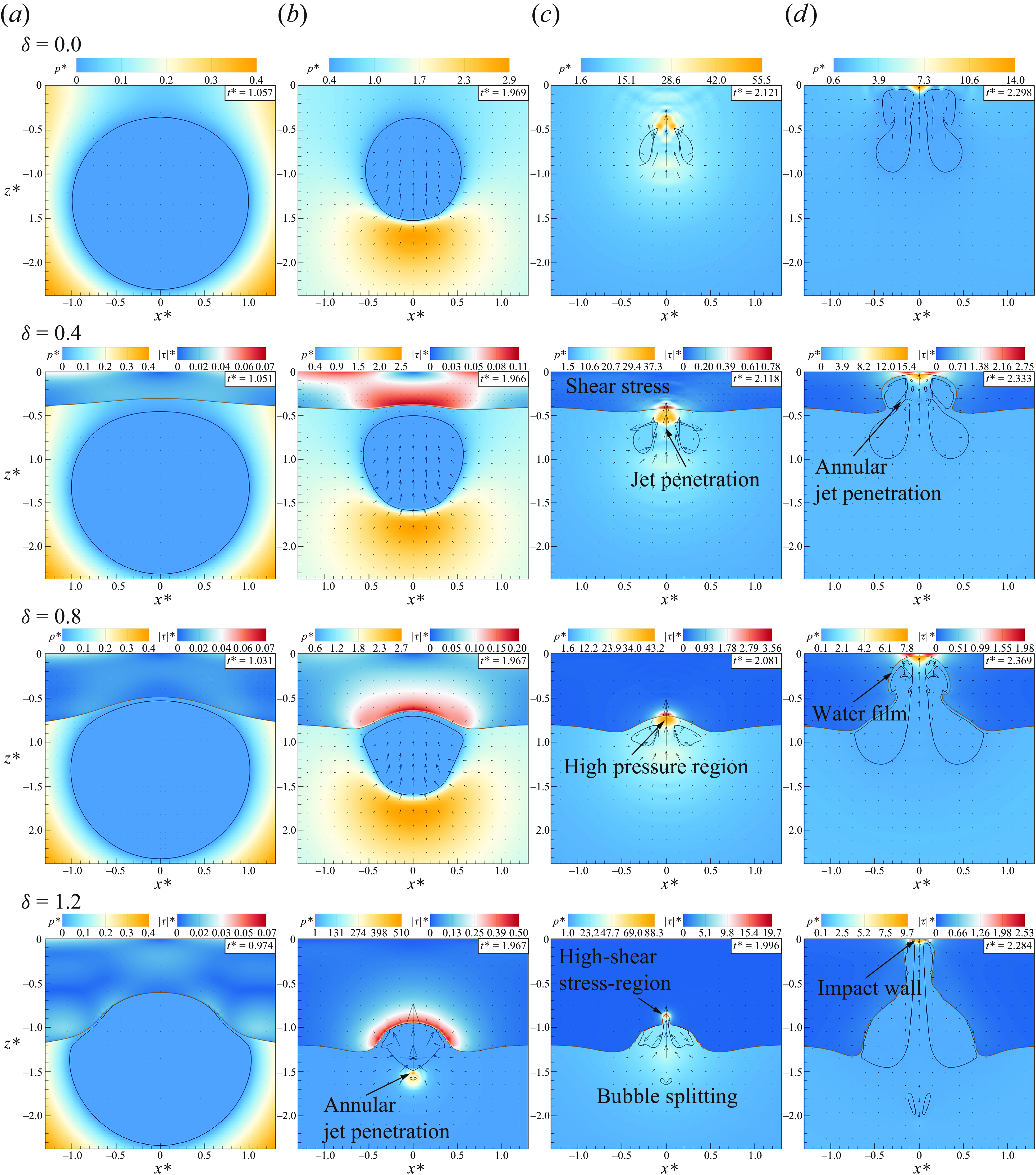
Figure 9. Evolution of bubbles and silicone-oil interface for different oil-layer thicknesses $\delta =0.0,0.4,0.8,1.2$
, at
$\delta =0.0,0.4,0.8,1.2$
, at $\gamma =1.3$
,
$\gamma =1.3$
, $\mu ^*=0.065$
.
$\mu ^*=0.065$
.
Figure 9 illustrates the collapse process of bubbles near oil layers of varying thicknesses ( $\mu ^*=0.065$
), including the maximum bubble radius, annular jet impact, jet penetration, and jet impacting on the wall, and also compares with the situation without a viscous oil layer (
$\mu ^*=0.065$
), including the maximum bubble radius, annular jet impact, jet penetration, and jet impacting on the wall, and also compares with the situation without a viscous oil layer ( $ \delta =0.0$
). In figure 9(a), notable differences in bubble shape arise at
$ \delta =0.0$
). In figure 9(a), notable differences in bubble shape arise at $\delta =1.2$
, where shear stress from the oil layer impede the upper portion of the bubble, resulting in a reduced expanded volume compared with the lower portion. Bubbles near thin oil layers have minimal contact with the oil layer during expansion. During bubble collapse, those with
$\delta =1.2$
, where shear stress from the oil layer impede the upper portion of the bubble, resulting in a reduced expanded volume compared with the lower portion. Bubbles near thin oil layers have minimal contact with the oil layer during expansion. During bubble collapse, those with $\delta =1.2$
produce a necking effect and an annular jet, generating a strong high-pressure region upon impact, dividing the bubble into two parts, each forming upward and downward jets. In contrast, the bubble near thinner layers or pure wall did not exhibit annular jets, but there were significant differences in bubble shape. In figure 9(c), the time of bubble-jet impact decreases with increasing oil-layer thickness for all cases. Following jet impact, high-pressure and high-shear-stress regions form in water and the oil layer, respectively. Peak pressures and shear stresses increase with oil-layer thickness, with peak pressure ratios of 1.16 and 2.04, and shear stress ratios of 4.56 and 5.53 for the three cases with viscous layers, respectively. There is a greater difference in shear stress, mainly due to higher-speed jets near thick oil layers, resulting in a more concentrated energy distribution. Upon bubble rebound, annular tearing occurs for bubbles with
$\delta =1.2$
produce a necking effect and an annular jet, generating a strong high-pressure region upon impact, dividing the bubble into two parts, each forming upward and downward jets. In contrast, the bubble near thinner layers or pure wall did not exhibit annular jets, but there were significant differences in bubble shape. In figure 9(c), the time of bubble-jet impact decreases with increasing oil-layer thickness for all cases. Following jet impact, high-pressure and high-shear-stress regions form in water and the oil layer, respectively. Peak pressures and shear stresses increase with oil-layer thickness, with peak pressure ratios of 1.16 and 2.04, and shear stress ratios of 4.56 and 5.53 for the three cases with viscous layers, respectively. There is a greater difference in shear stress, mainly due to higher-speed jets near thick oil layers, resulting in a more concentrated energy distribution. Upon bubble rebound, annular tearing occurs for bubbles with $\delta =0.4$
in figure 9(d), but not observed for
$\delta =0.4$
in figure 9(d), but not observed for $\delta =0.8$
and
$\delta =0.8$
and $1.2$
. Comparing scenarios figures 9(d) and 9(c), the jet width decreases significantly with increasing oil-layer thickness.
$1.2$
. Comparing scenarios figures 9(d) and 9(c), the jet width decreases significantly with increasing oil-layer thickness.
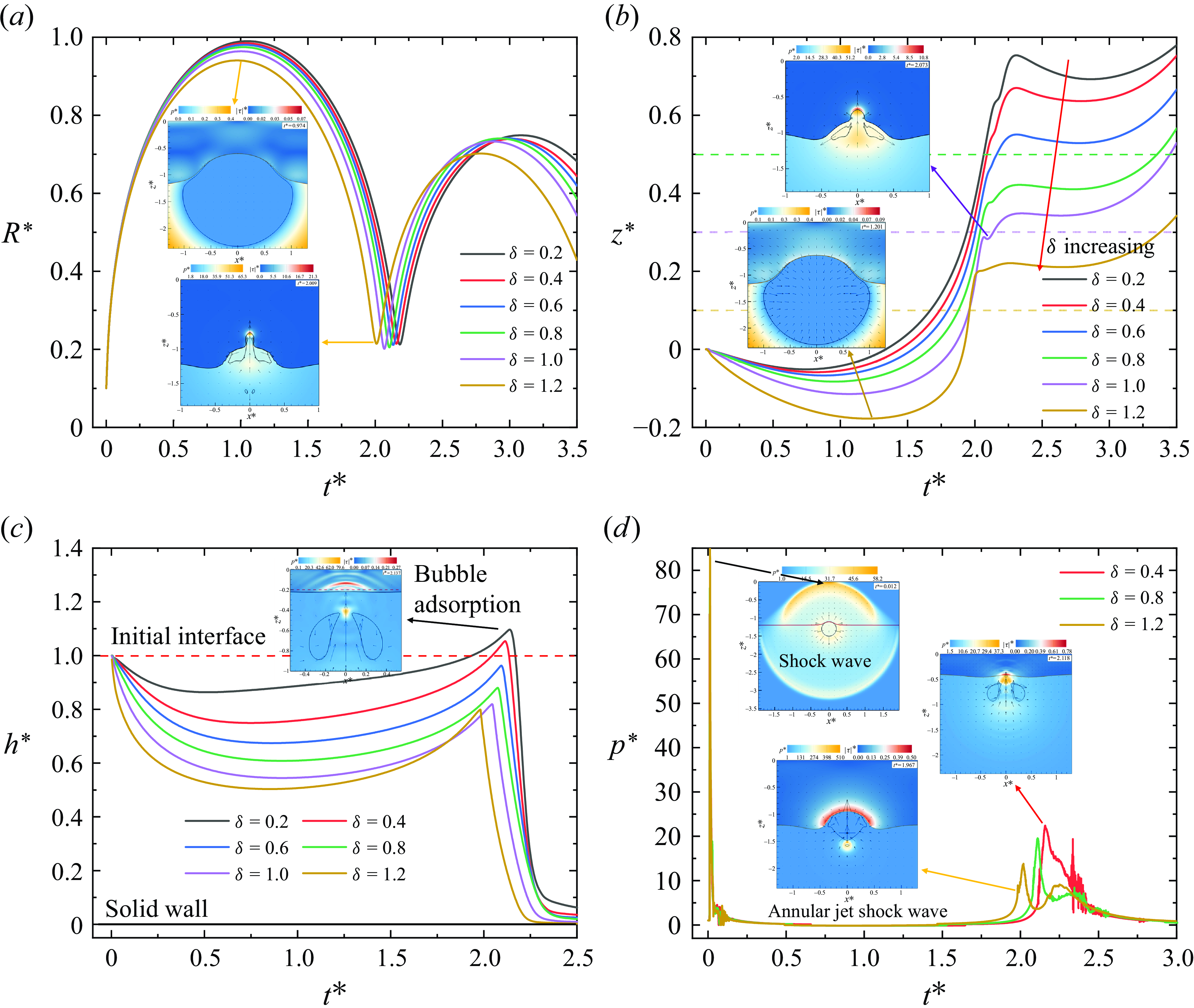
Figure 10. Time evolution for (a) bubble radius, (b) centre of mass position, (c) oil-layer thickness, (d) wall centre pressure at oil-layer thickness $\delta =$
0.2–1.2, stand-off distance
$\delta =$
0.2–1.2, stand-off distance $\gamma =1.3$
, viscosity
$\gamma =1.3$
, viscosity $\mu ^*=$
0.065.
$\mu ^*=$
0.065.
Figure 10 illustrates the evolution of the bubble radius, migration of the mass centre, normalised oil-layer thickness, and the central pressure load on the rigid wall across various oil-layer thicknesses. In comparison with low-viscosity silicone oil (see § 3.2.1), the dynamics of bubbles exhibits significant variations with changes in the oil layer. In figure 10(a), the bubble period decreases as the oil layer thickens, with relative reductions of 1.1 %, 1.1 %, 1.3 %, 1.8 % and 2.8 %, respectively. With increasing oil-layer thickness, the distance between the bubble and oil diminishes, augmenting the hindrance of bubbles by silicone oil. The initial bubble’s mass centre shifts away from the rigid wall and oil layer, with migration speed and magnitude significantly increasing as the oil layer thickens. Near the $\delta =1.2$
oil layer, the maximum bubble migration reaches 0.178, benefiting from the repulsion exerted by the oil layer. The horizontal dashed line in figure 10(b) denotes the position of the oil–water interface under corresponding operational conditions. Bubbles at
$\delta =1.2$
oil layer, the maximum bubble migration reaches 0.178, benefiting from the repulsion exerted by the oil layer. The horizontal dashed line in figure 10(b) denotes the position of the oil–water interface under corresponding operational conditions. Bubbles at $\delta$
= 1.0 and 1.2 enter the oil layer upon jet penetration, with subsequent bubble pulsation primarily occurring in the oil–water mixture, crucial for emulsifying the oil. The oil layer has an impact on the migration of bubbles towards the wall surface and exerts an indirect influence on the load at the wall surface, thereby reducing the impact of the pulsating load of the bubbles. During the first pulsation period (
$\delta$
= 1.0 and 1.2 enter the oil layer upon jet penetration, with subsequent bubble pulsation primarily occurring in the oil–water mixture, crucial for emulsifying the oil. The oil layer has an impact on the migration of bubbles towards the wall surface and exerts an indirect influence on the load at the wall surface, thereby reducing the impact of the pulsating load of the bubbles. During the first pulsation period ( $t^*\lt 2$
), the steeply rising curve segment at
$t^*\lt 2$
), the steeply rising curve segment at $\delta =1.2$
indicates rapid bubble migration. Combining with figure 9, it becomes evident that bubble migration in this phase depends on bubble collapse and jet, with the high-speed annular collapsing jet assuming a more pivotal role under the
$\delta =1.2$
indicates rapid bubble migration. Combining with figure 9, it becomes evident that bubble migration in this phase depends on bubble collapse and jet, with the high-speed annular collapsing jet assuming a more pivotal role under the $\delta =1.2$
condition.
$\delta =1.2$
condition.
Combining with figure 10(c) illustrates the evolution of the normalised thickness of the oil layer, displaying an initial decrease followed by an increase in thickness. The thickness decreases in various cases as $\delta$
increases. In contrast to the low-viscosity cases, for
$\delta$
increases. In contrast to the low-viscosity cases, for $\delta =0.2$
and
$\delta =0.2$
and $0.4$
, the rebound thickness of the oil layer surpasses the initial thickness due to bubble adsorption. This phenomenon, termed weak adsorptive collapse by Tang et al. (Reference Tang, Tian, Ju, Feng, Zhang and Zhang2023) in the examination of the interaction between explosion bubbles and non-Newtonian fluids, correlates with the distance between bubbles and oil layers as well as the viscosity of the oil layer. Changes in pressure at the centre of the rigid wall are also recorded, shown in figure 10(d). As pressure waves propagate in the liquid at nearly the speed of sound, and the speed of sound in silicone oil is lower than that in water, the shock-wave load at the wall centre lags with an increase in
$0.4$
, the rebound thickness of the oil layer surpasses the initial thickness due to bubble adsorption. This phenomenon, termed weak adsorptive collapse by Tang et al. (Reference Tang, Tian, Ju, Feng, Zhang and Zhang2023) in the examination of the interaction between explosion bubbles and non-Newtonian fluids, correlates with the distance between bubbles and oil layers as well as the viscosity of the oil layer. Changes in pressure at the centre of the rigid wall are also recorded, shown in figure 10(d). As pressure waves propagate in the liquid at nearly the speed of sound, and the speed of sound in silicone oil is lower than that in water, the shock-wave load at the wall centre lags with an increase in $\delta$
. During the initial two pulsation cycles, the centre pressure of the rigid wall also exhibits four significant characteristics: shock-wave load, pressure-reflection-wave load, pulsation load and jet-impact load. Due to the penetration of annular jets, an additional high-pressure region forms below the
$\delta$
. During the initial two pulsation cycles, the centre pressure of the rigid wall also exhibits four significant characteristics: shock-wave load, pressure-reflection-wave load, pulsation load and jet-impact load. Due to the penetration of annular jets, an additional high-pressure region forms below the $\delta =1.2$
oil layer, as indicated in the subgraph of figure 10(d). However, as the annular impact takes place beneath the bubble, the bubble obstructs the propagation of the shock wave. Despite the considerable impact pressure (
$\delta =1.2$
oil layer, as indicated in the subgraph of figure 10(d). However, as the annular impact takes place beneath the bubble, the bubble obstructs the propagation of the shock wave. Despite the considerable impact pressure ( $p^*=510$
), it does not induce significant disturbance in the pressure curve at the wall measurement point. When the jet collides with the rigid wall, the low-viscosity oil layer experiences a more pronounced slamming pressure.
$p^*=510$
), it does not induce significant disturbance in the pressure curve at the wall measurement point. When the jet collides with the rigid wall, the low-viscosity oil layer experiences a more pronounced slamming pressure.
3.3. Bubble dynamics with different silicone-oil viscosities
This section investigates the influence of silicone-oil viscosity on bubble dynamics and pressure load. The initial bubble parameters mirror those of § 3.2, with an initial bubble–wall distance set at $\gamma =1.3$
. Our focus was on an oil-layer thickness of
$\gamma =1.3$
. Our focus was on an oil-layer thickness of $\delta =0.8$
, and numerical simulations were conducted across silicone-oil viscosities ranging from
$\delta =0.8$
, and numerical simulations were conducted across silicone-oil viscosities ranging from $\mu ^*=0.0065$
to
$\mu ^*=0.0065$
to $0.39$
.
$0.39$
.
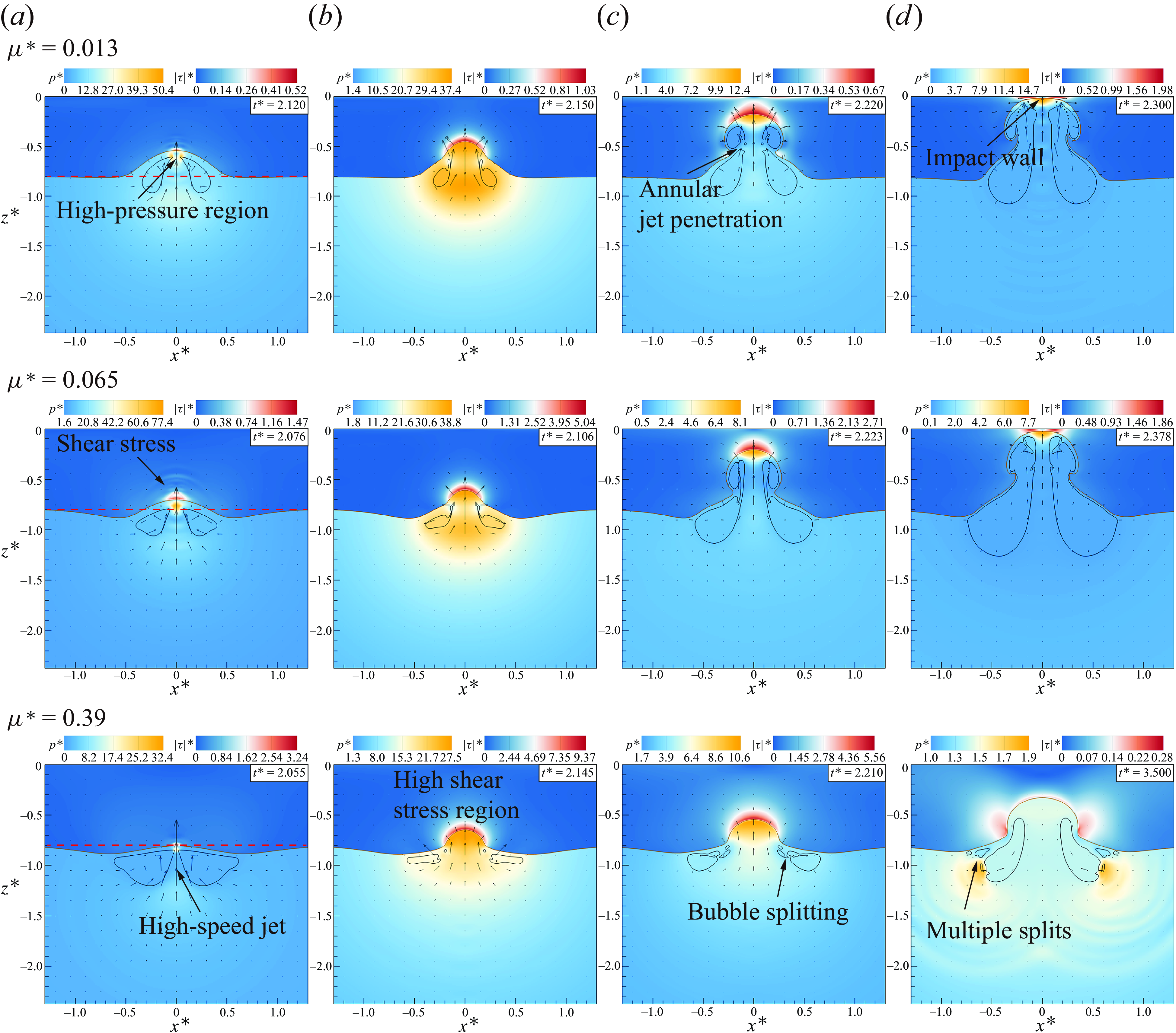
Figure 11. Evolution of bubbles and silicone-oil interface with different viscosities of silicone oils, at $\delta =0.8$
, stand-off distance
$\delta =0.8$
, stand-off distance $\gamma =1.3$
.
$\gamma =1.3$
.
Figure 11 illustrates four significant stages of bubble evolution across three viscosity conditions: initial jet penetration, minimum volume, annular tearing, and jet impact on the wall. With a substantial increase in viscosity, variations in bubble collapse shapes become apparent. In figure 11(a), jet penetration occurs earlier as the oil-layer viscosity increases. With the highest viscosity condition, the bubble is notably repelled by the oil layer, remaining above it during jet penetration (above the red dashed line), forming a butterfly-shaped annular bubble profile, and exerting an attractive force on the oil layer. As the bubble collapses further, it enters the low-viscosity oil layer and slides along the surface of the high-viscosity oil layer, as depicted in figure 11(b). The jet’s entry into the oil layer induces a zone of high shear stress. In figure 11(c), at an oil-layer viscosity of $\mu ^*=0.013$
, most of the bubble has entered the oil layer, leading to annular splitting. Conversely, for viscosity
$\mu ^*=0.013$
, most of the bubble has entered the oil layer, leading to annular splitting. Conversely, for viscosity $\mu ^*=0.39$
, the bubble persists near the oil layer’s surface, with larger bubbles fragmenting into multiple smaller ones. Bubbles with viscosities
$\mu ^*=0.39$
, the bubble persists near the oil layer’s surface, with larger bubbles fragmenting into multiple smaller ones. Bubbles with viscosities $\mu ^*=0.013$
and
$\mu ^*=0.013$
and $0.065$
penetrate the oil layer, impacting the wall at
$0.065$
penetrate the oil layer, impacting the wall at $t^*=2.3$
and
$t^*=2.3$
and $2.378$
, respectively. However, bubbles near the oil layer with viscosity
$2.378$
, respectively. However, bubbles near the oil layer with viscosity $\mu ^*=0.39$
do not reach the rigid wall, leaving only an impact pit in the oil layer. At medium viscosities, along with increased oil-layer thickness, collapsing bubble edges undergo significant curvature deformation, resulting in pinch-off similar to that observed in figure 9(c), a phenomenon commonly encountered in scenarios where the bubble–oil distance very small.
$\mu ^*=0.39$
do not reach the rigid wall, leaving only an impact pit in the oil layer. At medium viscosities, along with increased oil-layer thickness, collapsing bubble edges undergo significant curvature deformation, resulting in pinch-off similar to that observed in figure 9(c), a phenomenon commonly encountered in scenarios where the bubble–oil distance very small.
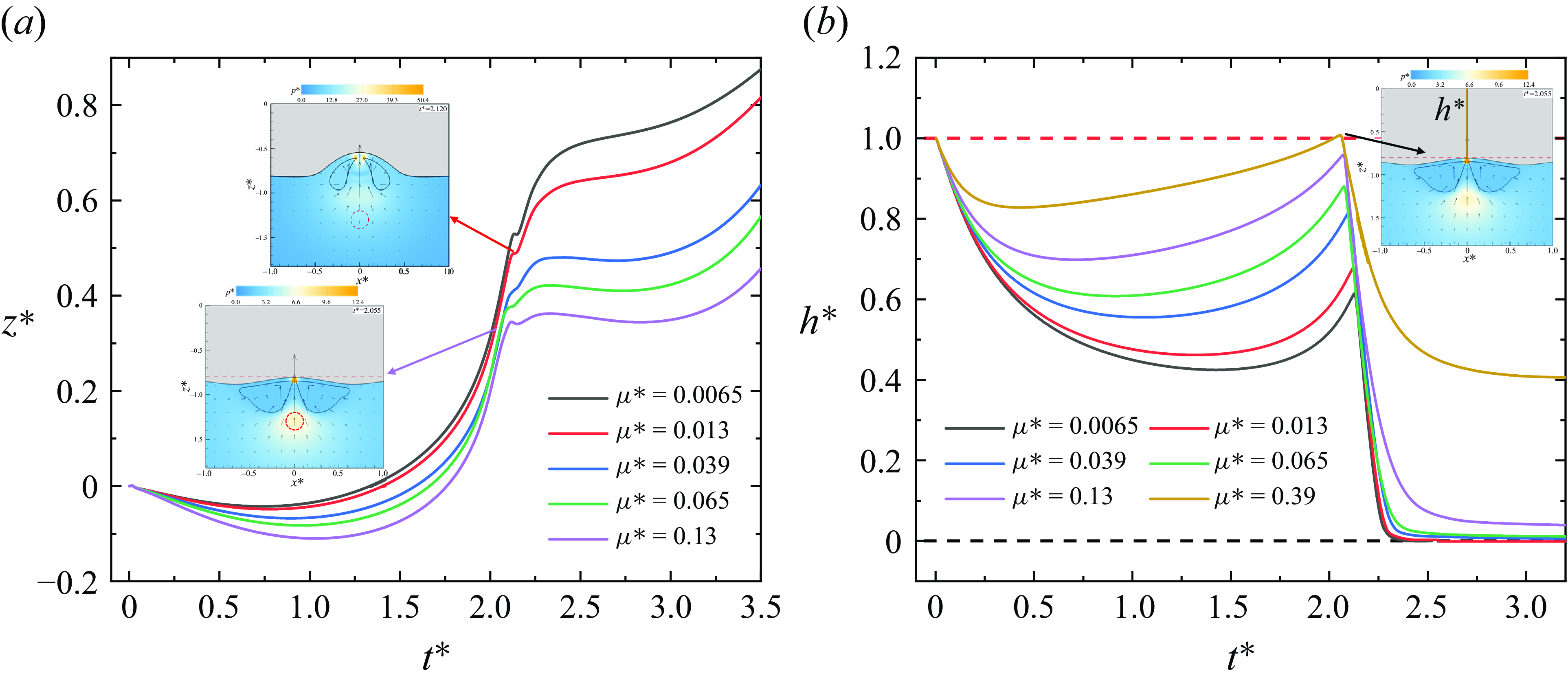
Figure 12. Time evolution for (a) centre of mass position, (b) oil-layer thickness at $\mu ^*=0.0065{-}0.39$
,
$\mu ^*=0.0065{-}0.39$
, $\gamma =1.3$
,
$\gamma =1.3$
, $\delta =0.8$
.
$\delta =0.8$
.
Figure 12 illustrates the evolution of both the centre of mass of bubbles and the thickness of oil layers under varying viscosity conditions. In figure 12(a), it is evident that as the viscosity increases, bubble migration is significantly reduced. At higher viscosity, the bubble can hardly penetrate the oil layer during pulsation, tending to remain near the oil–water interface. Furthermore, a rebound effect observed during bubble-jet penetration causes the bubble’s centre of mass to move downward. The subfigure in figure 12(a), which compares the positions of bubbles at $\mu ^*=0.013$
and
$\mu ^*=0.013$
and $0.13$
to their initial positions (red dashed line), effectively illustrates the displacement of bubbles and the barrier posed by the high-viscosity oil layer. Figure 12(b) shows the normalised thickness of the oil layer, indicating a decreasing trend in the rate of change of the oil-layer thickness with increasing viscosity. In current cases, the oil layers with
$0.13$
to their initial positions (red dashed line), effectively illustrates the displacement of bubbles and the barrier posed by the high-viscosity oil layer. Figure 12(b) shows the normalised thickness of the oil layer, indicating a decreasing trend in the rate of change of the oil-layer thickness with increasing viscosity. In current cases, the oil layers with $\mu ^*=0.13$
and
$\mu ^*=0.13$
and $\mu ^*=0.39$
have not disappeared, while the depth of impact craters formed by the bubble jet on the oil layer with
$\mu ^*=0.39$
have not disappeared, while the depth of impact craters formed by the bubble jet on the oil layer with $\mu ^*=0.39$
is merely
$\mu ^*=0.39$
is merely $0.6\delta$
. The evolutionary diagram of the oil–water interface, presented in figure 13(a) at viscosities of
$0.6\delta$
. The evolutionary diagram of the oil–water interface, presented in figure 13(a) at viscosities of $\mu ^*=0.065$
and
$\mu ^*=0.065$
and $0.39$
, aids in understanding the dynamic changes in the oil layer due to jet impact. Both viscosities result in the formation of a relatively wide pit under the jet’s impact, while areas not directly impacted by the jet are elevated due to the adsorption effect of the bubbles. In the oil layer with
$0.39$
, aids in understanding the dynamic changes in the oil layer due to jet impact. Both viscosities result in the formation of a relatively wide pit under the jet’s impact, while areas not directly impacted by the jet are elevated due to the adsorption effect of the bubbles. In the oil layer with $\mu ^*=0.065$
, the interface moves continuously towards the wall during ongoing bubble pulsations, eventually impacting the wall. In contrast, the oil layer with
$\mu ^*=0.065$
, the interface moves continuously towards the wall during ongoing bubble pulsations, eventually impacting the wall. In contrast, the oil layer with $\mu ^*=0.39$
shows the greatest displacement without direct wall contact. The viscosity reduces high-curvature deformations at the interfaces; the interface at
$\mu ^*=0.39$
shows the greatest displacement without direct wall contact. The viscosity reduces high-curvature deformations at the interfaces; the interface at $\mu ^*=0.39$
is smoother, whereas the oil layer at
$\mu ^*=0.39$
is smoother, whereas the oil layer at $\mu ^*=0.065$
shows a curling effect on the sidewalls.
$\mu ^*=0.065$
shows a curling effect on the sidewalls.
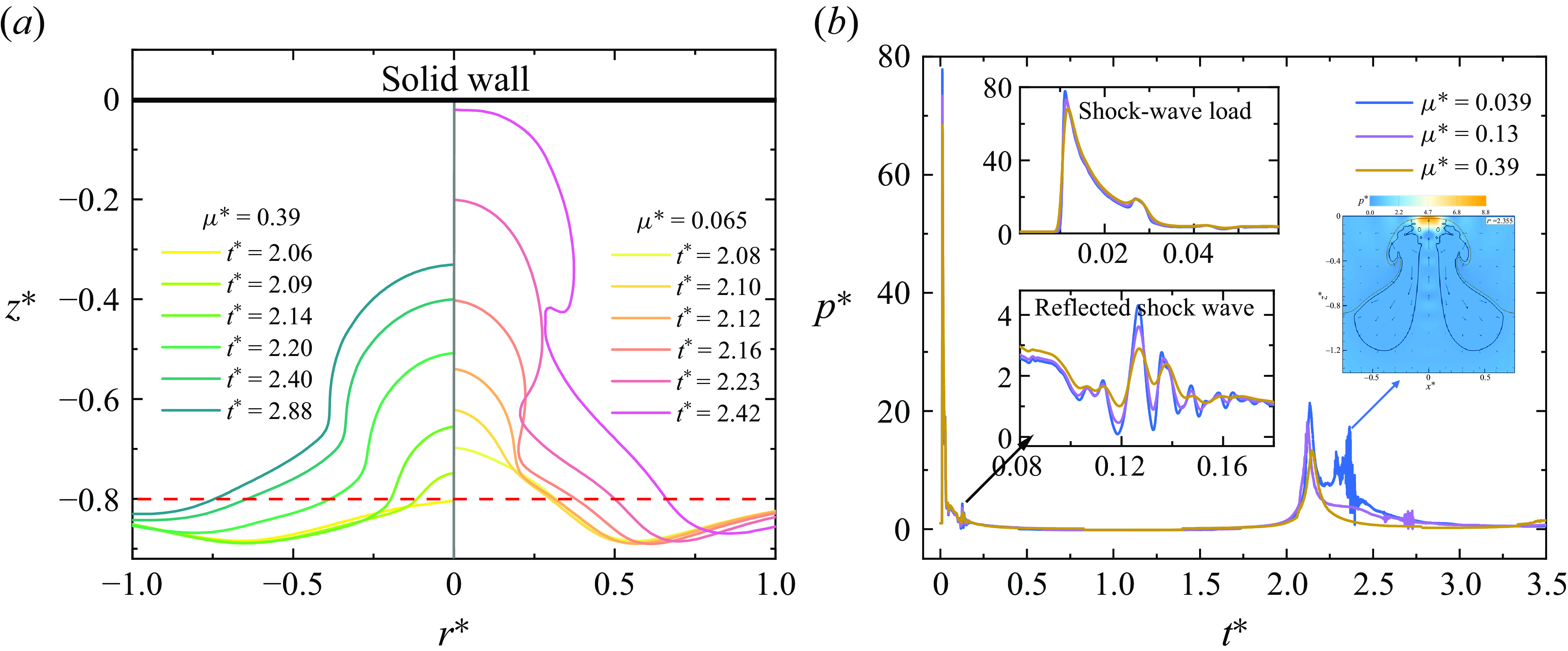
Figure 13. (a) Evolution of silicone-oil interface at $\mu ^*=0.065$
and
$\mu ^*=0.065$
and $0.39$
, the black line is the solid wall, and the red dashed line is the initial interface. (b) Evolution for wall centre pressure at
$0.39$
, the black line is the solid wall, and the red dashed line is the initial interface. (b) Evolution for wall centre pressure at $\mu ^*=$
0.039, 0.13, 0.39.
$\mu ^*=$
0.039, 0.13, 0.39.
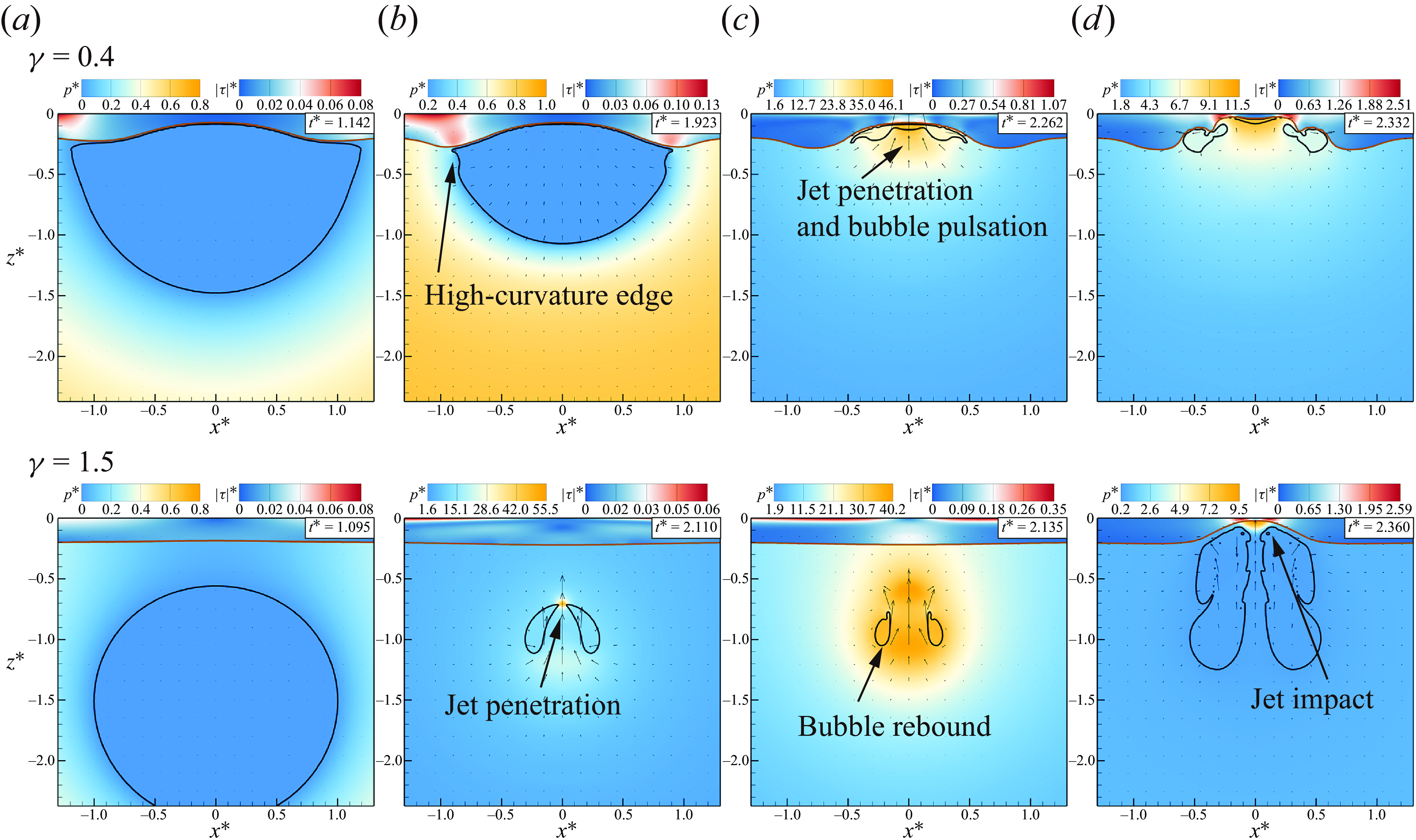
Figure 14. Evolution of bubbles and silicone-oil interface with different stand-off distances, at $\delta =0.2$
,
$\delta =0.2$
, $\mu ^*=0.065$
.
$\mu ^*=0.065$
.
Figure 13(b) illustrates the evolution of the central wall pressure over time. The viscosity reduces both impact- and reflective-wave loads, leading to a decrease in pulsating pressure with increasing viscosity. However, the timing of these pulsations does not vary monotonically with viscosity, indicating non-monotonic changes in the bubble period. At $t^* = 0.1$
, fluctuations in pressure emerged, which was attributed to the reflection of the shock wave between the wall and the two-phase interface. Although the reflected pressure was not substantial, repeated impacts would still exert an influence on the erosion of the wall. In the present cases, due to bubbles not being able to penetrate higher-viscosity oil layers and the collapsing jet failing to reach the rigid wall, the pressure load curve under high viscosity does not display jet-impact pressure.
$t^* = 0.1$
, fluctuations in pressure emerged, which was attributed to the reflection of the shock wave between the wall and the two-phase interface. Although the reflected pressure was not substantial, repeated impacts would still exert an influence on the erosion of the wall. In the present cases, due to bubbles not being able to penetrate higher-viscosity oil layers and the collapsing jet failing to reach the rigid wall, the pressure load curve under high viscosity does not display jet-impact pressure.
3.4. Bubble dynamics with different stand-off distances
For wall load, bubble-induced shock waves, jets and pulsations exhibit distinct modes of action. Specifically, shock waves are characterised by high peak values but have a short duration, reflecting off the wall surfaces. Bubble jets primarily generate water hammer pressures, which may be lower in magnitude compared with shock waves, yet they persist for longer durations and can direct transient pressure stagnation points. Shock waves attenuate with distance during propagation; therefore, the distance between the bubble and the wall is critical for wall load. Additionally, greater distances between the bubble and the wall also reduce jet intensity. In this section, a silicone-oil layer with a viscosity of $\mu ^* = 0.065$
and a thickness of
$\mu ^* = 0.065$
and a thickness of $\delta = 0.2$
is selected, and the scenarios where the stand-off distance ranges from 0.4 to 2.0 are explored. As depicted in figure 14, two cases with stand-off distances of 0.4 and 1.5 are presented, and the distinctions in bubble-pulsation behaviour and viscous-layer variations are quite evident. The bubble with a stand-off distance of 0.4 assumes a semicircular shape when it expands to the maximum radius, which is rather similar to the bubble shape near the wall (Reuter et al. Reference Reuter, Zeng and Ohl2022b
). The difference is that the upper surface of the bubble will be immersed in a viscous liquid and take the form of an arc. In contrast, the bubble with a stand-off distance of
$\delta = 0.2$
is selected, and the scenarios where the stand-off distance ranges from 0.4 to 2.0 are explored. As depicted in figure 14, two cases with stand-off distances of 0.4 and 1.5 are presented, and the distinctions in bubble-pulsation behaviour and viscous-layer variations are quite evident. The bubble with a stand-off distance of 0.4 assumes a semicircular shape when it expands to the maximum radius, which is rather similar to the bubble shape near the wall (Reuter et al. Reference Reuter, Zeng and Ohl2022b
). The difference is that the upper surface of the bubble will be immersed in a viscous liquid and take the form of an arc. In contrast, the bubble with a stand-off distance of $\gamma = 1.5$
remains nearly spherical throughout the expansion process, indicating a weaker influence of the oil layer on the bubble’s shape. At this distance, the bubble still generates a jet directed towards the wall, and the jet penetration occurs before the bubble rebounds. When
$\gamma = 1.5$
remains nearly spherical throughout the expansion process, indicating a weaker influence of the oil layer on the bubble’s shape. At this distance, the bubble still generates a jet directed towards the wall, and the jet penetration occurs before the bubble rebounds. When $\gamma = 0.4$
, the bubble jet approximately occurs concurrently with the bubble’s rebound, and the load acting on the wall is the superposition of the jet-impact load and the bubble-pulsation load. Subsequently, the bubble expands in the vicinity of the wall and enters the second cycle. The jet of the bubble with a stand-off distance
$\gamma = 0.4$
, the bubble jet approximately occurs concurrently with the bubble’s rebound, and the load acting on the wall is the superposition of the jet-impact load and the bubble-pulsation load. Subsequently, the bubble expands in the vicinity of the wall and enters the second cycle. The jet of the bubble with a stand-off distance $\gamma =1.5$
does not reach and impact the wall until
$\gamma =1.5$
does not reach and impact the wall until $t^* = 2.36$
. Due to the larger distance, the velocity decays significantly and the jet-impact load is relatively small. Subsequently, we still conducted analyses on the displacement of the bubble’s centre of mass and the pressure on the wall, as shown in figure 15. During the expansion phase, all bubbles move away from the wall–oil-layer direction and the degree of migration decreases with increasing stand-off distance. This is readily understandable as the asymmetric boundary leads to the asymmetric expansion of the bubble. Subsequently, the bubble generates a jet and rapidly moves towards the wall direction, and an inflection point emerges at
$t^* = 2.36$
. Due to the larger distance, the velocity decays significantly and the jet-impact load is relatively small. Subsequently, we still conducted analyses on the displacement of the bubble’s centre of mass and the pressure on the wall, as shown in figure 15. During the expansion phase, all bubbles move away from the wall–oil-layer direction and the degree of migration decreases with increasing stand-off distance. This is readily understandable as the asymmetric boundary leads to the asymmetric expansion of the bubble. Subsequently, the bubble generates a jet and rapidly moves towards the wall direction, and an inflection point emerges at $t^* = 2$
. The bubble continues to migrate downward for some time, and this instant corresponds to the minimum radius of the bubble. The migration law of the bubble during the rebound remains the same as in the initial expansion phase. In general, when the stand-off distance is less than 1.5, the migration of the bubble varies monotonically with the distance.
$t^* = 2$
. The bubble continues to migrate downward for some time, and this instant corresponds to the minimum radius of the bubble. The migration law of the bubble during the rebound remains the same as in the initial expansion phase. In general, when the stand-off distance is less than 1.5, the migration of the bubble varies monotonically with the distance.
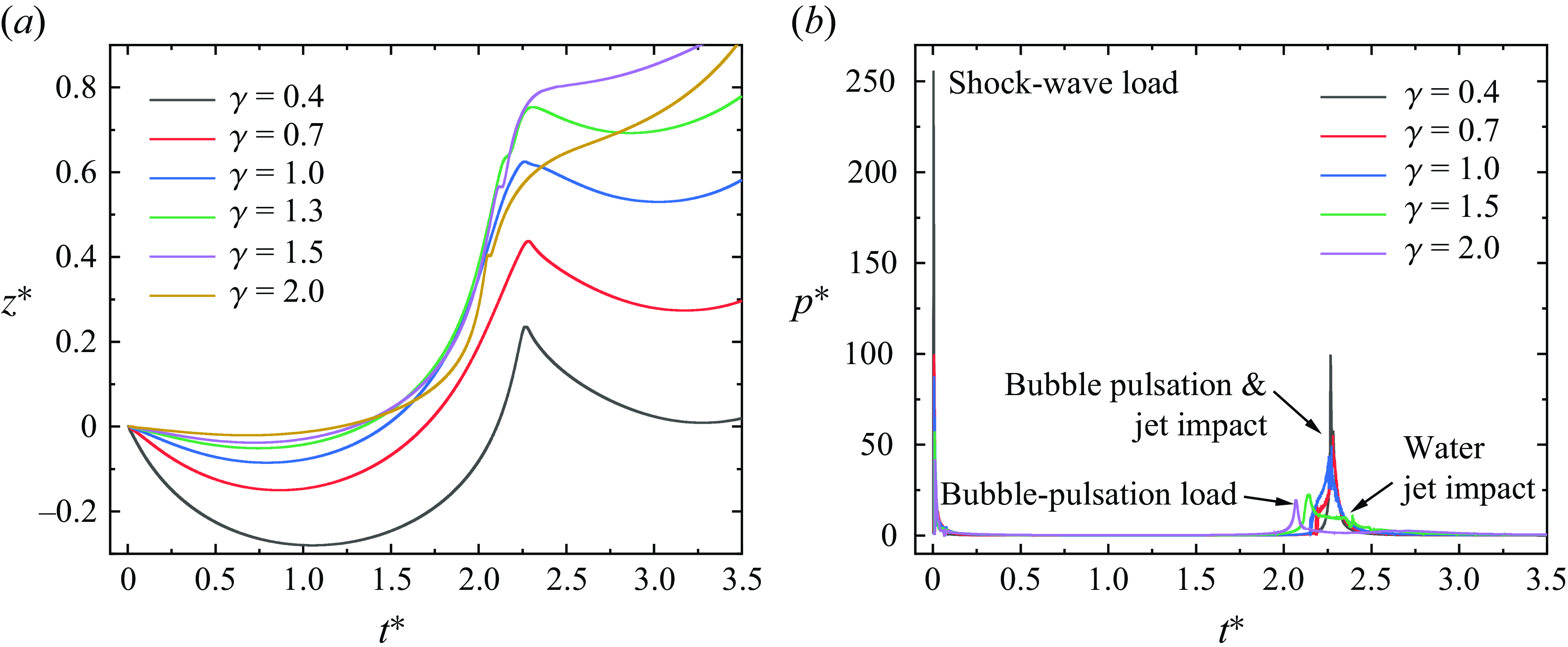
Figure 15. Time evolution for (a) centre of mass position, (b) wall centre pressure at $\mu ^*=0.065$
,
$\mu ^*=0.065$
, $\delta =0.2$
,
$\delta =0.2$
, $\gamma =0.4{-}2.0$
.
$\gamma =0.4{-}2.0$
.
In figure 15(b), the shock-wave load decreases as the distance parameter increases, consistent with the expected attenuation of shock waves over stand-off distance. This behaviour is similar to that observed for bubbles near a rigid wall and does not highlight the influence of the viscous oil layer. This also succinctly indicates that in terms of the impact erosion of cavitation bubbles, the distance between bubble walls is of great significance. During the subsequent bubble-collapse phase, the pressure-load characteristics on the wall become more complex. Generally, the pressure load decreases as the stand-off distance increases; however, the load distribution varies significantly at different distances. When the stand-off distance $\gamma$
is less than 1.0, the timing of the bubble-pulsation pressure and jet-impact pressure is nearly simultaneous, leading to their superposition and resulting in a higher wall load. This peak load can approach the peak shock-wave pressure (e.g.
$\gamma$
is less than 1.0, the timing of the bubble-pulsation pressure and jet-impact pressure is nearly simultaneous, leading to their superposition and resulting in a higher wall load. This peak load can approach the peak shock-wave pressure (e.g. $\gamma= 0.7$
). In contrast, at larger
$\gamma= 0.7$
). In contrast, at larger $\gamma$
, there is a noticeable time lag between the jet load and bubble-collapse load, which are reflected separately on the pressure-evolution curve. From this analysis and data comparison, it is evident that the distance between bubbles significantly influences the bubble–wall–oil-layer system. However, by contrasting with previous literature (Wang et al. Reference Wang, Liu, Zhang and Sui2015; Reuter et al. Reference Reuter, Zeng and Ohl2022b
), we find that the effect of distance on the bubble–wall–oil-layer system mirrors that on the bubble–wall system, indicating that the role of the viscous oil layer is minimal. The same law is also applicable to the initially thicker oil layer.
$\gamma$
, there is a noticeable time lag between the jet load and bubble-collapse load, which are reflected separately on the pressure-evolution curve. From this analysis and data comparison, it is evident that the distance between bubbles significantly influences the bubble–wall–oil-layer system. However, by contrasting with previous literature (Wang et al. Reference Wang, Liu, Zhang and Sui2015; Reuter et al. Reference Reuter, Zeng and Ohl2022b
), we find that the effect of distance on the bubble–wall–oil-layer system mirrors that on the bubble–wall system, indicating that the role of the viscous oil layer is minimal. The same law is also applicable to the initially thicker oil layer.
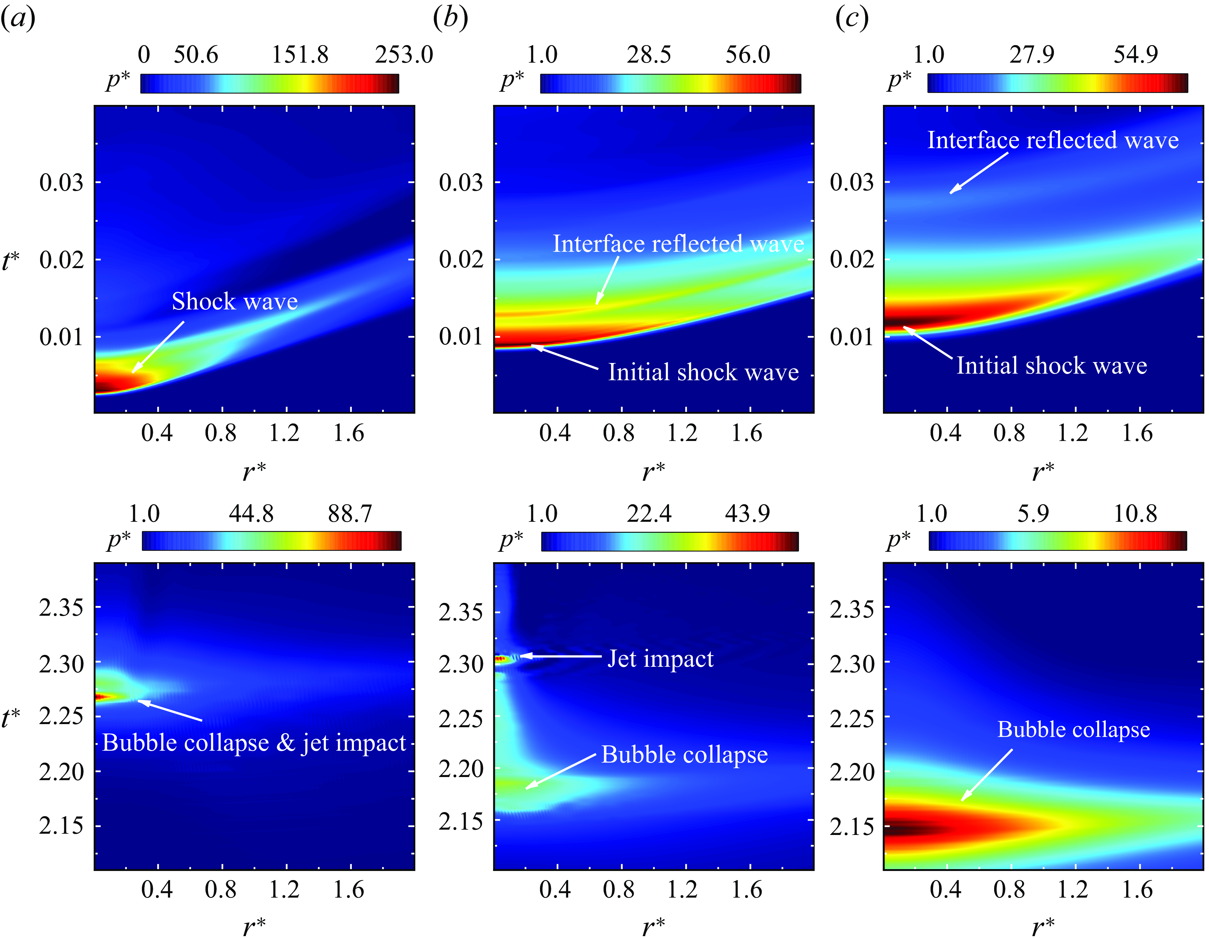
Figure 16. Spatio–temporal wall pressure during the shock-wave stage (upper image) and the bubble-collapse stage (lower image) at (a) $\gamma =0.4$
,
$\gamma =0.4$
, $\delta =0.2$
,
$\delta =0.2$
, $\mu ^*=0.13$
; (b)
$\mu ^*=0.13$
; (b) $\gamma =1.3$
,
$\gamma =1.3$
, $\delta =0.2$
,
$\delta =0.2$
, $\mu ^*=0.0065$
; (c)
$\mu ^*=0.0065$
; (c) $\gamma =1.3$
,
$\gamma =1.3$
, $\delta =0.8$
,
$\delta =0.8$
, $\mu ^*=0.39$
.
$\mu ^*=0.39$
.
To enhance understanding of pressure-distribution characteristics on a wall, the spatio–temporal pressure distribution on a rigid wall is illustrated in figure 16. Three distinct cases were employed for comparative illustration of the functional effects of viscosity, thickness and stand-off distance. In figure 16, the three graphs in the upper part depict the spatio–temporal distribution of wall pressure during the initial shock wave phase. For figure 16(a), considering that the bubble is the closest to the wall, the shock wave initially reaches the wall, and simultaneously, the pressure peak is the highest. Comparing figure 16(b) with figure 16(c), given the identical initial stand-off distance, the shock wave reaches the wall in figure 16(b) earlier. This is because the propagation speed of the shock wave in oil is slower than that in water, thereby requiring more time to pass through a thicker oil layer. At approximately $t^* = 0.013$
, a secondary pressure peak appears on the wall in figure 16(b) due to the reflected pressure wave at the oil–water interface undergoing a second reflection, which then impacts the wall and generates the secondary peak. This reflected wave may intensify the damage to the wall caused by the shock wave. In thicker and more viscous layers (figure 16
c), the secondary peak occurs later and is of lower magnitude because the viscous layer increases the wave propagation distance and dissipates the wave energy.
$t^* = 0.013$
, a secondary pressure peak appears on the wall in figure 16(b) due to the reflected pressure wave at the oil–water interface undergoing a second reflection, which then impacts the wall and generates the secondary peak. This reflected wave may intensify the damage to the wall caused by the shock wave. In thicker and more viscous layers (figure 16
c), the secondary peak occurs later and is of lower magnitude because the viscous layer increases the wave propagation distance and dissipates the wave energy.
In the bubble-collapse stage, the three highly typical load patterns on the wall are depicted in the lower graphs of figure 16. In figure 16(a), merely one prominent pressure peak emerges. Based on the previous analysis, this is the combined consequence of bubble-collapse and jet-impingement loads. In the second case, as depicted in figure 16(b), the bubble-collapse load occurs initially, followed by the jet impact. The rationale behind this is that the jet velocity is lower than the shock-wave velocity, and the jet reaches and impinges on the wall only after the bubble rebounds to a certain degree. Figure 16(c) presents the third situation, namely, when the oil layer is particularly thick or the viscosity is substantial, the jet virtually fails to impinge on the wall, and the wall merely receives a relatively minor bubble-collapse load. Furthermore, there is another situation not presented here, namely that the jet load precedes the bubble-collapse load, which typically occurs at a smaller stand-off distance and when the viscous effect is not prominent.
Figure 17. (a) Phase diagram of bubble-period distribution under different oil-layer conditions when $\gamma = 1.3$
, where
$\gamma = 1.3$
, where $T_{{wall}}=2.165$
represents the bubble-pulsation period without oil layer at the same stand-off distance (reference period) and
$T_{{wall}}=2.165$
represents the bubble-pulsation period without oil layer at the same stand-off distance (reference period) and $T_{oil}$
represents the bubble period when there is an oil layer. The downward-pointing triangles represent
$T_{oil}$
represents the bubble period when there is an oil layer. The downward-pointing triangles represent $T_{oil} \lt T_{wall}$
, and the upward-pointing triangles represent
$T_{oil} \lt T_{wall}$
, and the upward-pointing triangles represent $T_{oil} \gt T_{wall}$
. The red triangles are Ohl et al. (Reference Ohl, Reese and Ohl2024) results and the purple triangles are the experimental results. (b) Graph of the combined function relationship between bubble period
$T_{oil} \gt T_{wall}$
. The red triangles are Ohl et al. (Reference Ohl, Reese and Ohl2024) results and the purple triangles are the experimental results. (b) Graph of the combined function relationship between bubble period $T^*$
and
$T^*$
and $\delta$
and
$\delta$
and $\mu ^*$
, with the black line indicating the envelope line of the period distribution.
$\mu ^*$
, with the black line indicating the envelope line of the period distribution.
After investigating the collapse, migration and deformation of the oil layer, as well as the impact of wall load on viscosity and oil-layer thickness, we discovered that the bubble period varies non-monotonically with changes in these two parameters. Therefore, we expanded the range of viscosity parameters selected to study the variation law of the bubble period. From the above analysis, we can find that the effect of the stand-off distance on the bubble–wall–oil-layer system is the same as that on the bubble–wall system. Therefore, there is no need to repeat the study of the stand-off distance. Here, we still select a distance parameter $\gamma = 1.3$
and study the periodic changes of the bubble by altering the thickness and viscosity of the oil layer. This helps us to understand the pulsating-load law on the wall. The non-monotonic variation of the bubble-pulsation period under special conditions was mentioned in the previous text, and it is difficult for us to clarify the reason. Here, the period of a pulsating bubble near a pure wall with a stand-off distance of 1.3 is used as a reference period to study the effect of the oil-layer conditions on the bubble-pulsation frequency. As shown in figure 17(a), the distributional phase diagram of the bubble period is obtained by comparing it with the reference period and combining the viscosity and thickness of the oil layer. There is a clear boundary between the two cases of bubble periods, which is linear in the logarithmic coordinate system and can be expressed as
$\gamma = 1.3$
and study the periodic changes of the bubble by altering the thickness and viscosity of the oil layer. This helps us to understand the pulsating-load law on the wall. The non-monotonic variation of the bubble-pulsation period under special conditions was mentioned in the previous text, and it is difficult for us to clarify the reason. Here, the period of a pulsating bubble near a pure wall with a stand-off distance of 1.3 is used as a reference period to study the effect of the oil-layer conditions on the bubble-pulsation frequency. As shown in figure 17(a), the distributional phase diagram of the bubble period is obtained by comparing it with the reference period and combining the viscosity and thickness of the oil layer. There is a clear boundary between the two cases of bubble periods, which is linear in the logarithmic coordinate system and can be expressed as $\delta =0.756+0.35\text{log}_{10} \mu ^*$
(it should be noted that all values here are dimensionless, so the effect of the units of the variables is not taken into account). Above the line, the bubble period associated with the oil layer is smaller than the reference period, indicating that the presence of the oil layer accelerates the bubble pulsation. The reasons for this are that the oil layer reduces the pulsation scale of the bubble, resulting in a shorter period. Conversely, when the viscosity of the oil layer is larger or the thickness of the oil layer is smaller, the bubble period increases instead. The reason is that the upper boundary of the bubble is dragged by the viscous oil layer during the contraction process, thereby reducing the collapse speed. Based on this boundary line, a new parameter
$\delta =0.756+0.35\text{log}_{10} \mu ^*$
(it should be noted that all values here are dimensionless, so the effect of the units of the variables is not taken into account). Above the line, the bubble period associated with the oil layer is smaller than the reference period, indicating that the presence of the oil layer accelerates the bubble pulsation. The reasons for this are that the oil layer reduces the pulsation scale of the bubble, resulting in a shorter period. Conversely, when the viscosity of the oil layer is larger or the thickness of the oil layer is smaller, the bubble period increases instead. The reason is that the upper boundary of the bubble is dragged by the viscous oil layer during the contraction process, thereby reducing the collapse speed. Based on this boundary line, a new parameter $\delta -0.35\text{log}_{10} \mu ^*$
is obtained by combining
$\delta -0.35\text{log}_{10} \mu ^*$
is obtained by combining $\delta$
and
$\delta$
and $\mu ^*$
, and the relationship between the new parameter and the period is plotted as shown in figure 17(b). The period can be enveloped by two straight lines, with the horizontal line representing the reference period. The intersection point of the envelope is the boundary point of the size relation between the bubble period and the reference period. The presence of the envelope region indicates that there is a range of variability in the bubble period, with definite bounds on the value of the bubble period except for approximately twice the Rayleigh collapse time.
$\mu ^*$
, and the relationship between the new parameter and the period is plotted as shown in figure 17(b). The period can be enveloped by two straight lines, with the horizontal line representing the reference period. The intersection point of the envelope is the boundary point of the size relation between the bubble period and the reference period. The presence of the envelope region indicates that there is a range of variability in the bubble period, with definite bounds on the value of the bubble period except for approximately twice the Rayleigh collapse time.
4. Conclusion
In this paper, we explore the motion of a cavitation bubble adjacent to a rigid wall with a viscous oil layer and the characteristics of the pressure load at the centre of the wall. The effects of the thickness of the viscous oil layer, the viscosity and the stand-off distance of the bubble–wall–oil-layer system are analysed separately. The principal conclusions thus obtained are as follows.
-
(i) The influence of the distance parameter
$\gamma$
on the wall-pressure law of the bubble–wall–oil-layer system is identical to that on the bubble–wall system, both diminishing with the increase of the distance parameter. When
$\gamma \lt 1.5$
, the bubble migration increases monotonically with
$\gamma$
; however, when
$\gamma$
is relatively large, the bubble migration no longer varies monotonically. -
(ii) Generally, the increase in the thickness or viscosity of the viscous layer results in the reduction of the bubble radius, migration and peak wall pressure. At
$\mu ^*=0.0065$
, the bubble period decreases with the increase of
$\delta$
, yet the minimum bubble radius is scarcely affected. At
$\mu ^*=0.065$
, the bubble shape changes significantly with
$\delta$
, and the jet occurrence time advances with the increase in thickness. At
$\mu ^*=0.39$
, the jet hardly penetrates the oil layer, and the bubble oscillates in the vicinity of the interface. -
(iii) In comparison with the pure wall condition under the same distance, in the
$\mu ^*$
,
$\delta$
coordinate system, there exists a boundary line satisfying the logarithmic relationship for the bubble period:
$\delta =0.756+0.35\text{log}_{10} \mu ^*$
; the bubble period is related to
$\delta -0.35\text{log}_{10} \mu ^*$
, and there is a definite boundary.


Acknowledgements
Professor Zeng Qingyun is acknowledged for his improvement in the experimental method and the helpful suggestions on the manuscript.
Funding
The work was supported by the National Natural Science Foundation of China under grant nos 12332014 and 51925904, and the Scientific Research Innovation Capability Support Project for Young Faculty (ZYGXQNJSKYCXNLZCXM-O1).
Declaration of Interests
The authors report no conflict of interest.


 Open access