


Impact Statement
To manage environmental problems, we need to understand where anthropogenic pressures are generated and who, or what, is driving the production of these pressures. For food production, this requires understanding who is consuming which foods and where those foods are produced. For the first time, we quantify these connections globally. A better understanding of the pressures of the global food system allows more accurate estimates of the environmental impact of food. We encourage the use of these pressure data by researchers who aim to ultimately understand the environmental impacts of food trade at national and sub-national scales. These data can be used in future economic, geographic, or environmental analyses.
1. Introduction
The global food system is responsible for approximately 30% of greenhouse gas (GHG) emissions, 40% of global land use, over 50% of nitrogen and phosphorus use, and 70% of water use (Rosegrant et al., Reference Rosegrant, Ringler and Zhu2009; Land Use in Agriculture by the Numbers, 2020; Crippa et al., Reference Crippa, Solazzo, Guizzardi, Monforti-Ferrario, Tubiello and Leip2021). These environmental pressures in turn have huge impacts on climate change, biodiversity loss, water quality, and water scarcity. We define environmental pressures as the processes, inputs, and outputs involved in the production of food (Judd et al., Reference Judd, Backhaus and Goodsir2015; Kuempel et al., Reference Kuempel, Frazier, Nash, Jacobsen, Williams, Blanchard, Cottrell, McIntyre, Moran, Bouwman, Froehlich, Gephart, Metian, Többen and Halpern2020). Accurately calculating the impact of a pressure relies on the sensitivity of a system to specific pressures (Halpern et al., Reference Halpern, Frazier, Verstaen, Rayner, Clawson, Blanchard, Cottrell, Froehlich, Gephart, Jacobsen, Kuempel, McIntyre, Metian, Moran, Nash, Többen and Williams2022).
To understand how we can manage and mitigate environmental pressures from the food system, past research has assessed and mapped them to the food production areas and the processes that generate them (Gephart et al., Reference Gephart, Henriksson, Parker, Shepon, Gorospe, Bergman, Eshel, Golden, Halpern, Hornborg, Jonell, Metian, Mifflin, Newton, Tyedmers, Zhang, Ziegler and Troell2021; Halpern et al., Reference Halpern, Frazier, Verstaen, Rayner, Clawson, Blanchard, Cottrell, Froehlich, Gephart, Jacobsen, Kuempel, McIntyre, Metian, Moran, Nash, Többen and Williams2022). However, food production is ultimately driven by its consumption. Therefore, to manage the environmental pressures and subsequent impacts of food production, we need to understand where this food is also being consumed (Poore and Nemecek, Reference Poore and Nemecek2018).
The food system has become increasingly globalized: currently, about 25% of food consumed has been traded internationally, while 22% of all global trade by value is food (12% by weight) (D’Odorico et al., Reference D’Odorico, Carr, Laio, Ridolfi and Vandoni2014; Nyström et al., Reference Nyström, Jouffray, Norström, Crona, Søgaard Jørgensen, Carpenter, Bodin, Galaz and Folke2019). Therefore, understanding the teleconnections between where food is produced and where it is consumed is vital to managing its environmental impact (Halpern et al., Reference Halpern, Cottrell, Blanchard, Bouwman, Froehlich, Gephart, Sand Jacobsen, Kuempel, McIntyre, Metian, Moran, Nash, Többen and Williams2019). To date, comprehensive data on food production, the environmental pressures of food, and where foods are consumed have been siloed, and mismatches in the data scale and product resolution inhibit linking pressures of production to consumption. To address this data gap, we have completed the non-trivial task of combining the environmental pressures of food production with bilateral producer-to-consumer flow data, derived from trade data, to generate the most comprehensive assessment to date of the environmental pressures of food consumption globally, using freely accessible data.
This data product matches livestock, aquatic food, and crop trade and production with environmental pressures and links this production to the consuming nation. Pressures connected to the use of crops and fishmeal as feed were accounted for in the location and trade of pressures associated with animal production. We define food as substances “consisting essentially of protein, carbohydrate and (or) fat used in the body of an organism to sustain growth, repair and vital processes and to furnish energy” (Merriam–Webster). These data include the pressures and trade from food products that could also be used for non-food uses, such as fuel or fiber. A broad summary of the overall steps taken for our data output is outlined in Figure 1. Details of these steps are described below.
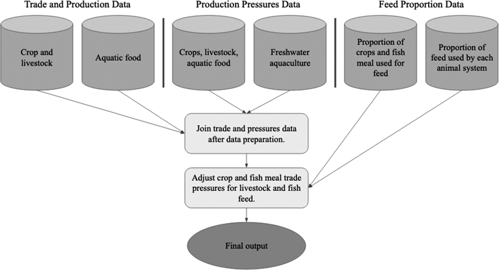
Figure 1. Conceptual diagram of the analytical workflow. Trade, environmental pressures, and feed proportion data inputs are represented by the cylinders. The rectangles represent processing steps that lead to the final data output. The oval represents the final data output.
2. Trade and production data
Using trade and production data in concert can help connect where food production occurs to where it is consumed. Tracking trade is complicated because there are often intermediate trade partners, including foreign processing of products that can ultimately return to where they were produced. Trade flows represent transactions between countries and trade records generally do not indicate the country that grew crops, raised, or caught animals. This is because when products are imported and processed (i.e., undergo “substantial transformation”), they become a product of the processing nation. Therefore, in its raw format, trade data alone does not allow for production to be directly linked to consumption.
To link consumption to the country of production, we use bilateral trade data and production data in two ways. For crops and livestock, we build upon the methods from Schwarzmueller and Kastner (Reference Schwarzmueller and Kastner2022). This approach involves constructing an input–output matrix and calculating the Leontiff inverse. This model does not include aquatic foods, so we combine it with the Aquatic Resource Trade in Species (ARTIS) database. ARTIS estimates the species mix in exported products and the processing among product forms with an optimization model and links the solutions to bilateral trade data. Building upon these resources allowed us to generate our final dataset that links food consumption with the production pressures.
2.1. Crop and livestock trade and production data
To determine trade of crops and livestock, we built off the methodologies outlined in Schwarzmueller and Kastner (Reference Schwarzmueller and Kastner2022), first developed in Kastner et al. (Reference Kastner, Kastner and Nonhebel2011). These approaches track the production, imports, and exports of various food items. Data from the Food and Agriculture Organization of the United Nations (FAO) were obtained from FAOSTAT, the FAO’s statistical database, which includes trade (import and export volume) and production (volume) for each country. There are two separate databases: FAO trade data only record import and export of a food product from a given country, while production data record how much of a food product is produced in the country. Together, the trade and production datasets allow one to capture the total flow of goods. Live animal trade was not included in our assessment as it is complex to track and we did not have data available that captures it.
We used average trade and production values from 2015 to 2019 because trade and production can vary greatly year to year, with common reporting errors in any given year. An average smooths out this variation and potential reporting error, providing a more “typical” pattern of trade. Centering our trade data on 2017 also allowed us to align the trade analysis with the environmental pressures dataset (Halpern et al., Reference Halpern, Frazier, Verstaen, Rayner, Clawson, Blanchard, Cottrell, Froehlich, Gephart, Jacobsen, Kuempel, McIntyre, Metian, Moran, Nash, Többen and Williams2022) described below.
Trade data are reported as tonnes of product (e.g., fresh apples, dried apples, apple juice), exported and/or imported, depending on the item traded. Production data are reported as tonnes of primary product grown and harvested in a given year. To harmonize these datasets, we converted the trade data into the primary product units following Schwarzmueller and Kastner (Reference Schwarzmueller and Kastner2022), using primary product dry weight conversion factors from the FAO. For example, using conversion factors we converted the tonnes of wheat flour traded into equivalent tonnes of harvested wheat traded. Dry matter conversion ratios are used to convert products into their primary product equivalents through a mass balance conversion. FAO commodity conversion factors are not used to avoid adding weight back on to products and in a way “creating” mass in the conversion step. This avoids double counting for non-aquatic products and allows us to assign the appropriate production pressures to the product.
The FAO trade and production data could be used in tandem to calculate apparent consumption, building upon the work from Schwarzmueller and Kastner (Reference Schwarzmueller and Kastner2022) and Kastner et al. (Reference Kastner, Kastner and Nonhebel2011). Imports, exports, and production data are process through a trade matrix operation to calculate: “(1) import serving a country’s consumption, (2) export originating from a country’s production, as well as (3) consumption originating from a country’s own production” (Schwarzmueller and Kastner, Reference Schwarzmueller and Kastner2022). Equation (1) is a simplified example of the apparent consumption output generated from this operation. In a few cases (0.3% of total tonnes in the FAOSTAT data), exports exceed production plus imports due to differences in production and trade data, or production estimates that arise from converting traded products into primary commodity products. In these cases, the trade operation produces negative consumption values; we adjusted these to zero. Because these cases were rare and are generally very small values, this adjustment has a minimal effect on results.
 $$ {\mathrm{Consumption}}_{\mathrm{i},\mathrm{c}}={\mathrm{Production}}_{\mathrm{i},\mathrm{c}}+{\mathrm{Imports}}_{\mathrm{i},\mathrm{c}}-{\mathrm{Exports}}_{\mathrm{i},\mathrm{c}} $$
Equation (1). A simplification of the trade matrix operation from Schwarzmueller and Kastner (Reference Schwarzmueller and Kastner2022). For each item (i), it calculates a country’s (c) consumption of that item.
2.2. Aquatic food trade data
Aquatic food trade data were sourced from the ARTIS database, which includes over 2400 species/species groups from 193 countries, and over 35 million bilateral records ( Gephart et al. Reference Gephart, Agrawal Bejarano, Gorospe, Godwin, Golden, Naylor, Nash, Pace and Troell2024). ARTIS represents a disaggregation of reported aquatic product trade (e.g., frozen salmon filets) into species/species groups, with information on wild versus farmed sourcing. Species trade is estimated by modeling each country’s conversion of wild and farmed production into commodities, conversion of imported commodities through processing, and apparent consumption. Estimated species mixes and processing of foreign-sourced products are then connected to bilateral trade data to disaggregate flows of aquatic foods.
Instances where exports cannot be explained by domestic production and imports, or where trade moves through more than two intermediate countries, produce values in exports of unknown origin, representing about 8.6% of the total tonnes of aquatic food trade. To assign environmental pressures to flows of unknown source, we reclassified unknown flows proportionately to each consuming nation’s known aquatic food sourcing by source country, habitat, method, and species groups. Without this adjustment, pressures from aquatic foods, which are known to be traded, would be dropped, artificially lowering the pressures stemming from aquatic food consumption.
To distinguish aquatic food trade and consumption from fishmeal trade and use, we incorporated information on the production of fishmeal. Fishmeal is “ground dried fish and fish waste used as fertilizer and animal food” (Merriam–Webster). This was necessary because production data by species does not distinguish production for direct human consumption from industrial uses, including fishmeal. To do this, we first calculated total fishmeal production by country based on the FAO processed products data (FAO Fisheries & Aquaculture, n.d.). We then joined this with each country’s total imports and exports of fishmeal from ARTIS. Next, we calculated apparent consumption (production + imports - exports or Eq. (1)). We assume apparent consumption is sourced proportionally from imports and domestic production, so we calculated domestic fishmeal consumption (Eq. (2)) and foreign fishmeal consumption (Eq. (3)). For the foreign fishmeal, we then identified sourcing proportionally to each country’s fishmeal imports. Note that fish oil flows are not included in ARTIS as all co-products are excluded to avoid double-counting during the conversion to live weight.
 $$ \mathrm{Domestic}\ \mathrm{fishmeal}\ \mathrm{consumption}=\frac{\mathrm{production}}{\mathrm{production}+\mathrm{imports}}\times \mathrm{total}\ \mathrm{consumption} $$
 $$ \mathrm{Foreign}\ \mathrm{fishmeal}\ \mathrm{consumption}=\frac{\mathrm{imports}}{\mathrm{production}+\mathrm{imports}}\times \mathrm{total}\ \mathrm{consumption} $$
Equations (2) and (3). Calculating how much of fish meal consumption comes from domestic and foreign fish meal sources.
3. Production pressures data
For the purposes of this analysis, the environmental pressures of food production specifically refer to within-farm-gate pressures and exclude the pressures from activities like processing, transportation, or manufacturing equipment (Halpern et al., Reference Halpern, Frazier, Verstaen, Rayner, Clawson, Blanchard, Cottrell, Froehlich, Gephart, Jacobsen, Kuempel, McIntyre, Metian, Moran, Nash, Többen and Williams2022). We process environmental pressures data primarily from Halpern et al. (Reference Halpern, Frazier, Verstaen, Rayner, Clawson, Blanchard, Cottrell, Froehlich, Gephart, Jacobsen, Kuempel, McIntyre, Metian, Moran, Nash, Többen and Williams2022), but since that did not include inland aquaculture, we supplement it with data from Gephart et al. (Reference Gephart, Henriksson, Parker, Shepon, Gorospe, Bergman, Eshel, Golden, Halpern, Hornborg, Jonell, Metian, Mifflin, Newton, Tyedmers, Zhang, Ziegler and Troell2021), to generate pressure values per tonne of production for each product and producing nation. The environmental pressures considered are GHG emissions (CO2eq), freshwater use (m3), land use (km2eq), and nutrient emissions (tonnes excess of N and P). Importantly, pressure does not presume impact, as the translation of pressures into impacts is highly dependent on local context. For example, land use impacts on biodiversity depend on the ecological context of the land being occupied (see Kuempel et al., Reference Kuempel, Frazier, Nash, Jacobsen, Williams, Blanchard, Cottrell, McIntyre, Moran, Bouwman, Froehlich, Gephart, Metian, Többen and Halpern2020 for details).
3.1. Crops, livestock, marine seafood, and freshwater fisheries data
The environmental pressures of food production have recently been assessed and mapped globally for most food groups (livestock, crops, wild fisheries, farmed seafood) and countries, covering 99% of total reported food production (Halpern et al., Reference Halpern, Frazier, Verstaen, Rayner, Clawson, Blanchard, Cottrell, Froehlich, Gephart, Jacobsen, Kuempel, McIntyre, Metian, Moran, Nash, Többen and Williams2022). Specific pressures assessed and mapped were GHG emissions, freshwater use, nitrogen and phosphorus (nutrient) pollution, and land/water disturbance, as well as the cumulative pressure from all four (see Halpern et al., Reference Halpern, Frazier, Verstaen, Rayner, Clawson, Blanchard, Cottrell, Froehlich, Gephart, Jacobsen, Kuempel, McIntyre, Metian, Moran, Nash, Többen and Williams2022 for full details). Here, we estimated environmental pressure efficiencies for each country and food product combination by dividing the total of each environmental pressure generated in each country by each food product by the total tonnes of production for that product in the country. We recalculated efficiencies (rather than using the total pressure values from Halpern et al., Reference Halpern, Frazier, Verstaen, Rayner, Clawson, Blanchard, Cottrell, Froehlich, Gephart, Jacobsen, Kuempel, McIntyre, Metian, Moran, Nash, Többen and Williams2022) to reduce the impacts of any differences in production data and our source data.
The calculated pressure efficiencies were capped at the third standard deviation from the mean of each product group (e.g., wheat, cows’ meat, etc.) and pressure (e.g., water) to reduce the effect of outliers when calculating total pressures traded. This capping was done because most of the outliers in the pressure data were from small-scale production systems, and keeping these outliers would inappropriately skew data output when multiplied by traded tonnes. For example, the disturbance pressure efficiency for freshwater fish production in Libya was four times larger than the capped value, while its production data used to calculate the efficiency totaled less than 1 tonne. The efficiencies that were capped total less than 2% of the efficiencies calculated from Halpern et al. (Reference Halpern, Frazier, Verstaen, Rayner, Clawson, Blanchard, Cottrell, Froehlich, Gephart, Jacobsen, Kuempel, McIntyre, Metian, Moran, Nash, Többen and Williams2022).
3.2. Freshwater aquaculture
Halpern et al. (Reference Halpern, Frazier, Verstaen, Rayner, Clawson, Blanchard, Cottrell, Froehlich, Gephart, Jacobsen, Kuempel, McIntyre, Metian, Moran, Nash, Többen and Williams2022) did not assess environmental pressures from freshwater aquaculture due to data limitations that arise when specifically mapping spatial footprints of specific food production. As we did not need high-resolution, sub-national maps of pressures for flows of pressures among nations, we used global average values of environmental pressures from GHG emissions, freshwater use, land use, and nutrient emissions for all freshwater aquaculture species included in the data from ARTIS (Gephart et al., Reference Gephart, Henriksson, Parker, Shepon, Gorospe, Bergman, Eshel, Golden, Halpern, Hornborg, Jonell, Metian, Mifflin, Newton, Tyedmers, Zhang, Ziegler and Troell2021). The pressure data in Gephart et al. (Reference Gephart, Henriksson, Parker, Shepon, Gorospe, Bergman, Eshel, Golden, Halpern, Hornborg, Jonell, Metian, Mifflin, Newton, Tyedmers, Zhang, Ziegler and Troell2021) represent a global average, so here we must assume environmental pressures per tonne from freshwater aquaculture are the same for every country. Since we know there is geographic variability in environmental performance, this is a priority for future improvements with better data. Gephart et al. (Reference Gephart, Henriksson, Parker, Shepon, Gorospe, Bergman, Eshel, Golden, Halpern, Hornborg, Jonell, Metian, Mifflin, Newton, Tyedmers, Zhang, Ziegler and Troell2021) provide more detailed information on how the environmental pressure efficiencies of freshwater aquaculture production were estimated.
Although Halpern et al. (Reference Halpern, Frazier, Verstaen, Rayner, Clawson, Blanchard, Cottrell, Froehlich, Gephart, Jacobsen, Kuempel, McIntyre, Metian, Moran, Nash, Többen and Williams2022) and Gephart et al. (Reference Gephart, Henriksson, Parker, Shepon, Gorospe, Bergman, Eshel, Golden, Halpern, Hornborg, Jonell, Metian, Mifflin, Newton, Tyedmers, Zhang, Ziegler and Troell2021) did not use the same methods for calculating environmental pressures, they considered the same set of pressures and both set the system boundaries as cradle-to-farm-gate. Environmental pressures for both sets of fish product data are expressed as environmental pressure per tonne, live weight equivalent.
4. Joining trade and pressures data
The process of connecting production/trade data with per-country pressure efficiency data varied for each food category, as the process depended on how well the food categories in the trade and pressure data matched. This process is summarized in Table 1 and detailed further below.
Table 1. Summary of how trade and environmental pressures data was joined
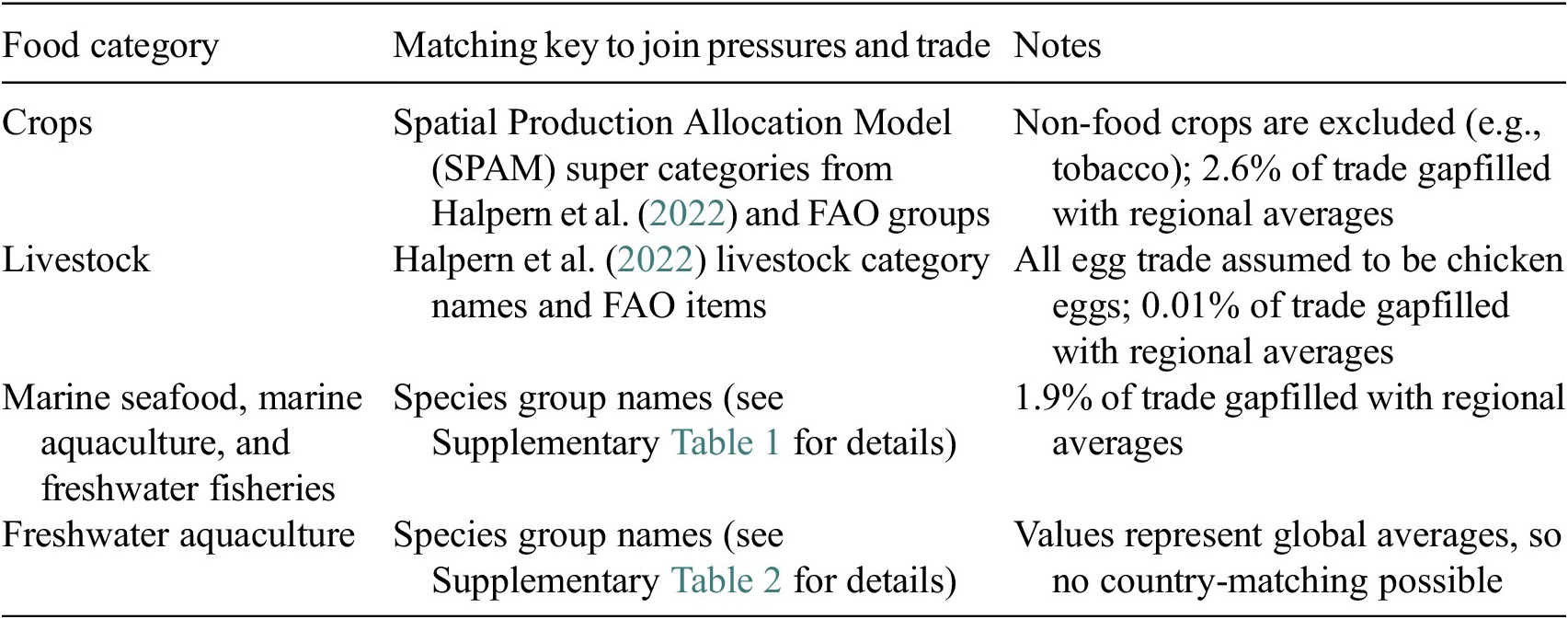
Crop trade and pressures were matched using the Spatial Production Allocation Model (SPAM) “super” categories from Halpern et al. (Reference Halpern, Frazier, Verstaen, Rayner, Clawson, Blanchard, Cottrell, Froehlich, Gephart, Jacobsen, Kuempel, McIntyre, Metian, Moran, Nash, Többen and Williams2022) and their corresponding FAO groups, as this was the finest resolution from the pressures data. SPAM is used to map crop production globally and uses FAOSTAT crop categories to generate these categories (Yu et al., Reference Yu, You, Wood-Sichra, Ru, Joglekar, Fritz, Xiong, Lu, Wu and Yang2020). Examples of crop categories include individual primary product forms like wheat, banana, or maize. Crop categories also include primary product aggregates like “vegetables” or “other cereals.” For the purposes of this publication, the “SPAM super” categories from Halpern et al. (Reference Halpern, Frazier, Verstaen, Rayner, Clawson, Blanchard, Cottrell, Froehlich, Gephart, Jacobsen, Kuempel, McIntyre, Metian, Moran, Nash, Többen and Williams2022) are referred to as SPAM categories. For more information on SPAM super categories, refer to the supplementary materials of Halpern et al. (Reference Halpern, Frazier, Verstaen, Rayner, Clawson, Blanchard, Cottrell, Froehlich, Gephart, Jacobsen, Kuempel, McIntyre, Metian, Moran, Nash, Többen and Williams2022).
A number of crop categories were not included in these data as they are not considered food for our purposes, and consequently, there was no associated pressure data (Halpern et al., Reference Halpern, Frazier, Verstaen, Rayner, Clawson, Blanchard, Cottrell, Froehlich, Gephart, Jacobsen, Kuempel, McIntyre, Metian, Moran, Nash, Többen and Williams2022). The excluded categories, and their SPAM titles, are other fiber crops (ofib), rest of crops (othr), teas (teas), tobacco (toba), and coffee (xcof). The FAO items “Mate” and “Chillies and peppers, green” were also excluded from the crops trade as there was no associated pressure data. Trade data for crops that are included in this study that did not have country-specific pressure efficiency data, but for which some pressure data existed for other countries, was gapfilled using United Nations (UN) intermediate region, UN subregion, or UN region averages of pressures for each food item category. UN regions, subregions, and intermediate regions were developed by the UN Statistical Division (UNSD) for “statistical convenience and does not imply any assumption regarding political or other affiliation of countries or territories…” (UNSD—Methodology, n.d.). 2.6% of total tonnes traded of crops were missing an associated pressure and gapfilled by this process.
Livestock trade and pressures were matched using corresponding names from the FAO and Halpern et al. (Reference Halpern, Frazier, Verstaen, Rayner, Clawson, Blanchard, Cottrell, Froehlich, Gephart, Jacobsen, Kuempel, McIntyre, Metian, Moran, Nash, Többen and Williams2022), such as cows’ meat, buffaloes’ milk, and so forth. All egg trade from the FAO was assigned the pressures for chicken eggs, as no other pressure data were available for eggs from other animals. As with crops, livestock trade data that did not have country-specific pressures were gapfilled using the same method. In the end, 0.01% of total tonnes traded of livestock were missing an associated pressure and gapfilled by this process.
Marine seafood, marine aquaculture, and freshwater fisheries trade data were matched by corresponding species group (see Supplementary Tables 1and 2 for species groupings). Gapfilling was done for this group in the same way as for crops. A total of 1.9% of tonnes traded of marine seafood, marine aquaculture, and freshwater fisheries were missing an associated pressure and gapfilled by this process. Freshwater aquaculture pressure efficiencies were already aggregated as global averages and were matched by species grouping. This food category required no gapfilling.
With trade and pressure efficiency data matched, we were able to calculate total pressures per country. Land, water, nutrient, and GHG pressure totals were calculated by multiplying the total tonnes traded by its pressure efficiency value for that food item and producing country.
5. Adjusting pressures for feed
To capture the full environmental pressures associated with the production of animal products, we needed to account for the fishmeal and crops that animal production uses (Figure 2). To do this, we assessed the proportion of crop and fishmeal used as feed within each country and each animal system. We estimated these proportions using a combination of FAOSTAT food balances and animal feed consumption quantities, using the process shown in Figure 3 (Halpern et al., Reference Halpern, Frazier, Verstaen, Rayner, Clawson, Blanchard, Cottrell, Froehlich, Gephart, Jacobsen, Kuempel, McIntyre, Metian, Moran, Nash, Többen and Williams2022; Schwarzmueller and Kastner, Reference Schwarzmueller and Kastner2022).
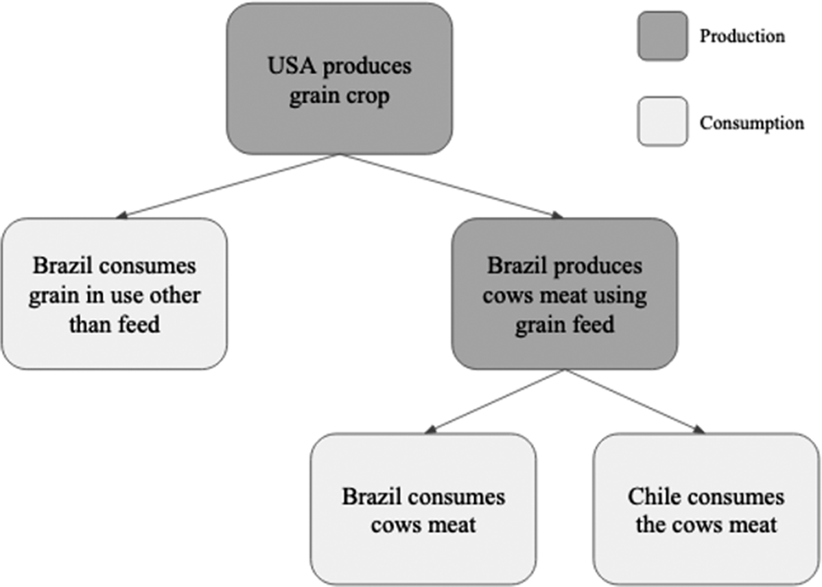
Figure 2. An example of how feed pressures can be traded and consumed as part of an animal product in different countries. In this scenario, grain imported from the United States of America (USA) is traded to Brazil and used either as feed for cows that are grown for meat or for direct consumption (i.e., not as feed). Once Brazil has grown and slaughtered the cows, they are either eaten in Brazil or traded to Chile for consumption there. The terminal (final) country is where the environmental pressures from the grain crop would be attributed.
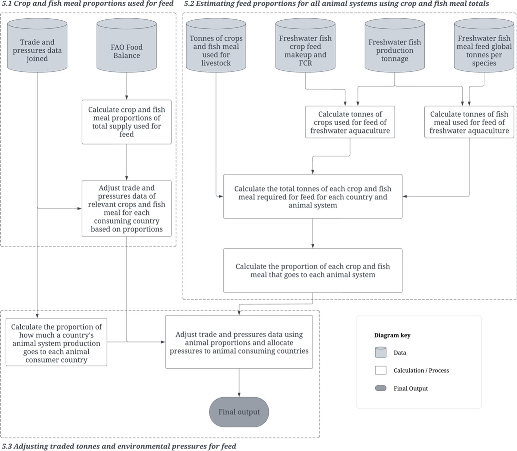
Figure 3. Flow diagram showing how trade and pressures data were adjusted for feed. In this flowchart we show how all of the steps described in the “adjusting for feed” section result in the final data output. Data are represented by the cylinders. The rectangles represent calculation and processing steps that lead to the final data output, represented by the oval.
5.1. Crop and fish meal proportions used for feed
We used FAOSTAT food balances data to determine a country’s proportion of crops used for feed. To do so, we first assigned which food groups are used for feed based on data from FAO and Halpern et al. (Reference Halpern, Frazier, Verstaen, Rayner, Clawson, Blanchard, Cottrell, Froehlich, Gephart, Jacobsen, Kuempel, McIntyre, Metian, Moran, Nash, Többen and Williams2022). These groups, and the SPAM categories within them, are summarized in Table 2. For the purposes of these data, all fishmeal trade and production were assumed to be used for feed because the data available was specifically for products not used for human consumption.
Table 2. Feed category crop group summaries
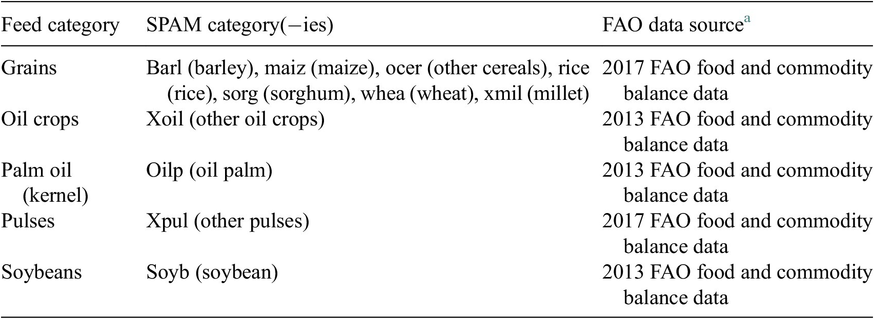
a 2013 FAO data were used for soy, palm oil, and oil crops because that is the most recent year in which data are available from the FAO that breaks down feed usage for these crops. The FAO changed reporting methodologies in 2013, which affected how some crops’ usage was tracked in their data.
For several crops (e.g., soy), feed comes from both the raw product and the “cake” that remains after oil extraction. These products are listed separately in the FAO database, and so we summed all “cake” production (assuming it was all used for feed) with the tonnes of raw product marked as feed. To estimate the proportion (rather than tonnage) of the crop used for feed, we then divided this summed value by the country’s domestic supply quantity from FAO Food Balance Sheets.
On average, across the five feed crop categories, 42% of countries did not have feed data available from the FAO. For these countries, we calculated averages at the level of UN-designated intermediate regions and used these to gapfill missing data (see Supplementary Table 3). When intermediate regions were unavailable, UN subregional, or if unavailable regional, averages were used to gapfill.
5.2. Estimating feed proportions for animal systems using crop and fish meal totals
We next estimated the proportion of the total feed supply of each crop within each country (calculated above) to each animal production system. As no country-specific data were available on the proportion of feed used for each system, we estimated these values using the total consumption of each feed category by each animal system and country. We estimated these totals for all animal systems except for freshwater aquaculture using data from Halpern et al. (Reference Halpern, Frazier, Verstaen, Rayner, Clawson, Blanchard, Cottrell, Froehlich, Gephart, Jacobsen, Kuempel, McIntyre, Metian, Moran, Nash, Többen and Williams2022).
Freshwater aquaculture was not included in Halpern et al. (Reference Halpern, Frazier, Verstaen, Rayner, Clawson, Blanchard, Cottrell, Froehlich, Gephart, Jacobsen, Kuempel, McIntyre, Metian, Moran, Nash, Többen and Williams2022); therefore, we calculated the total tonnes of crops and fishmeal used for these systems using estimates of feed makeup for species, feed conversion ratios (FCR), and tonnes of live weight production for a given species by each country (Eq. 4) (Gephart et al., Reference Gephart, Henriksson, Parker, Shepon, Gorospe, Bergman, Eshel, Golden, Halpern, Hornborg, Jonell, Metian, Mifflin, Newton, Tyedmers, Zhang, Ziegler and Troell2021). It is assumed that filter-feeding freshwater aquaculture species did not consume additional feed. We extracted country-specific live weight production data for freshwater aquaculture species from FAO data and calculated mean production values from 2015 to 2019 for each country. Live weight tonnes of production were summed for each species grouping for each country. We could then estimate the total tonnes of each feed component required to generate that production for each country by multiplying the species-specific FCR by the production level and the proportion of feed composed of each crop.
 $$ Tonnes\hskip0.32em {of\ feed}_{c,s}=\sum live\hskip0.32em {weight\ production}_s\times {FCR}_s\times {feed\ proportion}_{c,s} $$
Equation (4). Calculating the total tonnes of each crop (c) needed to produce a country’s freshwater aquaculture production for a given species (s).
The FAO data do not include tonnes of fishmeal used for freshwater aquaculture feed, so instead we used species-group-specific but global values from Froehlich et al. (Reference Froehlich, Jacobsen, Essington, Clavelle and Halpern2018). The global live weight of fishmeal used for each species was divided among countries based on the proportion of global production that a country is responsible for.
We next calculated the proportion of total tonnes of each crop and fishmeal that is used by each animal system in each country. To do this, we divided the tonnes of the feed category used by an animal by the feed category total (Eq. (5)). We then combined these feed proportions with the joined trade and pressures data.
 $$ {Proportion}_{f,a,c}=\frac{tonnes\hskip0.62em {of\ feed}_{f,a,c}}{\sum tonnes\hskip0.62em {of\ feed}_{f,c}} $$
Equation (5). Calculating the proportion of how much of a feed category (f) is used by a given animal system (a) for a specific country (c).
5.3. Adjusting traded tonnes and environmental pressures for feed
Finally, to complete the adjustment of pressures to account for feed, we combined the proportion of crop and fishmeal used as feed within each country and each animal system. We separated the feed crop SPAM categories (Table 2) and all of the fishmeal trade from the other trade and pressure data. Feed crop import trade was multiplied by the proportion of that crop used for feed by the crop-consuming country (calculated in Section 5.1). In the example from Figure 2, this is where we separate the grain imported from the USA by Brazil for feed and non-feed purposes.
Next, we multiplied the imported crop and fishmeal used for feed by a country by the proportion of that crop used for each animal system in the country (Section 5.2). This produced the tonnes traded and associated pressures of each crop and fishmeal used for feed, and how much is consumed by each animal system. In Figure 2, this is where we determine how much of the grain used for feed goes specifically toward cow’s meat.
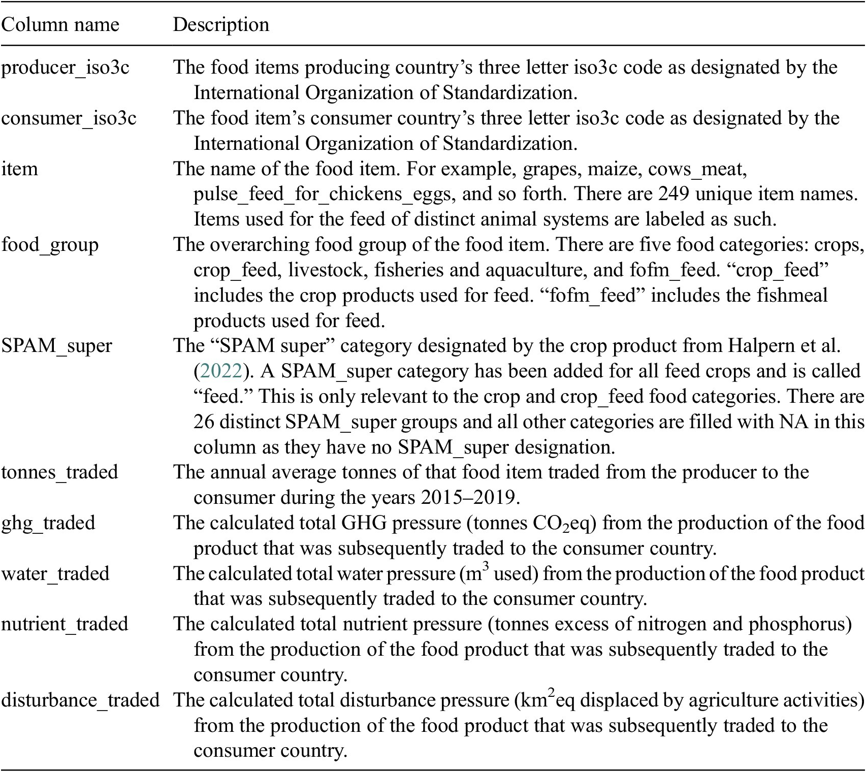
To assign environmental pressures to the animal-consuming country, we estimated the proportion of each animal system’s trade that came from each producer to each consumer country. The animal system trade proportions were then multiplied by the total crop consumption and associated pressures used for feed for each animal system by that country. The final output columns are summarized in Table 3.
Table 3. Summary of final data output columns
Abbreviations
- GHG
-
greenhouse gas
- ARTIS
-
Aquatic Resource Trade in Species
- FAO
-
Food and Agriculture Organization of the United Nations
- SPAM
-
Spatial Production Allocation Model
- UN
-
United Nations
- UNSD
-
United Nations Statistical Division
Open peer review
To view the open peer review materials for this article, please visit http://doi.org/10.1017/eds.2025.10009.
Acknowledgements
The authors would like to acknowledge Dr. Thomas Kastner for being gracious to answer multiple questions about their previous work’s methods. The details they provided helped push this research forward.
Supplementary material
The supplementary material for this article can be found at http://doi.org/10.1017/eds.2025.10009.
Author contribution
Conceptualization: B.S.H., D.R.W., K.L.N., J.A.G; Data curation: J.M.D., M.F., H.K.E., J.A.G; Funding acquisition: B.S.H.; Methodology: J.M.D., M.F., H.K.E., J.A.G; Writing—original draft: J.M.D.; Writing—review and editing: J.M.D., B.S.H., H.E.F, G.C., D.R.W., E.H.A., K.L.N., J.A.G. All authors approved the final submitted draft.
Competing interests
The authors declare no competing interests exist.
Data availability statement
The code used to develop this dataset are publicly available on GitHub at https://github.com/jagephart/food_trade_pressures. The data inputs and final output are publicly available on Zenodo at https://doi.org/10.5281/zenodo.10215132.
Ethical statement
The research meets all ethical guidelines, including adherence to the legal requirements of the study country.
Funding statement
This research was a collaborative endeavor conducted by the Environmental Justice Implications of Global Food Systems Working Group at the National Center for Ecological Analysis and Synthesis at the University of California Santa Barbara. Funding was provided by the Zegar Family Foundation (SB210274-Project 1). The National Center for Ecological Analysis and Synthesis at UC Santa Barbara provided invaluable infrastructural support for this work. E.H.A. was supported by donors to the CGIAR trust fund through the Resilient Aquatic Food Systems Initiative. J.A.G. was supported by the US National Science Foundation (#2121238).


 Open access
Comments
January, 12, 2024
Dear Editor:
Please accept the manuscript entitled “Development of a comprehensive bilateral trade-flow dataset of the environmental pressures of global food production” for consideration as a Data Paper in Environmental Data Science. This manuscript is original and research was conducted by the authors. In this paper we describe, in detail, the steps taken to produce a comprehensive dataset of bilateral trade flows of environmental pressures stemming from food production from producing to consuming nations. These data are novel and important because the environmental pressures from food production is significant, and understanding global consumption patterns is vital to managing environmental impacts. We expect these data to be used in future economic, geographic, or environmental analyses.
Three ways these data advance work in this field is:
1. It captures the bilateral environmental pressures trade of crops, livestock, feed, and seafood products. Similar data typically fails to capture the bilateral trade flows of all of these categories.
2. The data captures the trade of four separate environmental pressures in a single dataset: greenhouse gas emissions, water use, nitrogen and phosphorus pollution, and area of land/water occupancy of food production.
3. For all food sectors besides freshwater aquaculture, it uses environmental pressures data that are specific to the producing country and therefore captures the differences in production efficiency variability.
Upon publication the data, code, and supplementary materials that will reside in a publicly available Zenodo data repository. The code will also be available in a GitHub repository. Also included in the submission are three figures and three tables. No portion of this manuscript has been published in any form, and it has not been submitted elsewhere for consideration.
Sincerely, on behalf of all co-authors,
Joseph DeCesaro