


1. Introduction
The microscale manipulation of flowing fluids remains at the core of multiple modern applications, from microfluidic appliances in diagnostics and substance testing, to small-scale chemical synthesis and industrial precision manufacturing technologies. In Stokes flow conditions appropriate for sub-millimetre fluidic systems, flow can be controlled globally by imposing external forces or pressure gradients that induce laminar flow with only little mixing due to molecular diffusion. While easy to control, global forcing mechanisms pose challenges for applications that require local mixing, selective pumping, or the manipulation of suspended particles within confined environments (Squires & Quake Reference Squires and Quake2005). On the other hand, biological and nanorobotic actuation mechanisms, such as ciliated surfaces, rely on localised forcing to achieve swimming, pumping, mixing, nutrient capture, and sensing (Gilpin, Bull & Prakash Reference Gilpin, Bull and Prakash2020; Omori & Ishikawa Reference Omori and Ishikawa2025). In these settings, surface forcing becomes the key driver of macroscopic bulk flow. In confined geometry, such as in microchannels or pores, this mechanical activity is often coupled to the geometry of the flow domain, and the resulting asymmetry is responsible for creating flow.
A promising approach exploits phoretic mechanisms, in which surface-generated gradients (of concentration, temperature, etc.) induce effective slip flow on confining surfaces, which in turn gives rise to bulk flow (Anderson Reference Anderson1989). Diffusio-osmosis and diffusio-phoresis, the motion of particles and fluids in response to solute concentration gradients (Golestanian, Liverpool & Ajdari Reference Golestanian, Liverpool and Ajdari2007; Jülicher & Prost Reference Jülicher and Prost2009; Sabass & Seifert Reference Sabass and Seifert2012), is now a well-established active propulsion mechanism, with numerous applications in artificial active matter (Bechinger et al. Reference Bechinger, Di Leonardo, Löwen, Reichhardt, Volpe and Volpe2016; Shim Reference Shim2022).
The presence of local chemical gradients in microfluidic channels can lead to cooperation or competition with global advective flow, enabling size-dependent colloid transport (Shin et al. Reference Shin, Um, Sabass, Ault, Rahimi, Warren and Stone2016), or particle focusing that can be precisely tuned through the interplay of channel geometry, confinement, and surface chemical activity (Ault, Shin & Stone Reference Ault, Shin and Stone2018). Diffusio-phoresis has also been used to organise colloids into sharp bands (Staffeld & Quinn Reference Staffeld and Quinn1989), to boost the migration of large particles via imposed solute contrasts (Abécassis et al. Reference Abécassis, Cottin-Bizonne, Ybert, Ajdari and Bocquet2008), and to rectify particle motion to yield motility and pattern formation (Palacci et al. Reference Palacci, Abécassis, Cottin-Bizonne, Ybert and Bocquet2010). Subsequent microfluidic studies revealed steady-state focusing in multicomponent gradients (Shi et al. Reference Shi, Nery-Azevedo, Abdel-Fattah and Squires2016). In colloids–salt mixtures, phoretic effects were shown to affect mixing (Raynal & Volk Reference Raynal and Volk2019), potentially leading to flow effects ranging from enhanced dispersion to blockage in cellular flows (Volk et al. Reference Volk, Bourgoin, Bréhier and Raynal2022). The coupling of hydrodynamic flows and phoresis can further tune chemotactic and diffusio-phoretic spreading (Chu et al. Reference Chu, Garoff, Tilton and Khair2022).
In microscale channels, the presence of dead-end pores can be used to induce a concentration difference between the main channel and pores large enough to entrain particles (Wilson et al. Reference Wilson, Shim, Yu, Gupta and Stone2020), or capture and retain them (Battat et al. Reference Battat, Ault, Shin, Khodaparast and Stone2019; Akdeniz, Wood & Lammertink Reference Akdeniz, Wood and Lammertink2023), affecting filtration and dispersion in porous media (Alessio et al. Reference Alessio, Shim, Mintah, Gupta and Stone2021; Chu et al. Reference Chu, Garoff, Tilton and Khair2021; Doan et al. Reference Doan, Chun, Feng and Shin2021; Sambamoorthy & Chu Reference Sambamoorthy and Chu2023; Somasundar et al. Reference Somasundar, Qin, Shim, Bassler and Stone2023; Teng, Rallabandi & Ault Reference Teng, Rallabandi and Ault2023; Alipour et al. Reference Alipour, Li, Liu and Pahlavan2024; Jotkar et al. Reference Jotkar, de Anna, Dentz and Cueto-Felgueroso2024; Sambamoorthy & Chu Reference Sambamoorthy and Chu2025). Such diffusio-phoretic mechanisms have been shown to enhance solute and particle transport into and out of dead-end pores (Kar et al. Reference Kar, Chiang, Ortiz Rivera, Sen and Velegol2015), and to enable size-dependent control of colloidal trapping and release via solute gradients in confined geometries (Shin et al. Reference Shin, Um, Sabass, Ault, Rahimi, Warren and Stone2016), with recent simulations and analyses further quantifying phoretic transport and mixing in narrow channels (Bhattacharyya, Sengupta & Chakraborty Reference Bhattacharyya, Sengupta and Chakraborty2023; Migacz, Castleberry & Ault Reference Migacz, Castleberry and Ault2024; Visan, Wood & Lammertink Reference Visan, Wood and Lammertink2024). Active or catalytic pores have also been proposed as local pumps and mixers capable of driving sustained fluid transport without external pressure gradients (Antunes et al. Reference Antunes, Malgaretti, Harting and Dietrich2022, Reference Antunes, Malgaretti and Harting2023; Bhattacharyya et al. Reference Bhattacharyya, Sengupta and Chakraborty2023; Migacz et al. Reference Migacz, Castleberry and Ault2024; Tiwari et al. Reference Tiwari, Dhakar, Upadhyaya and Choudhary2025). When considering catalytic active surfaces, geometric asymmetry alone is sufficient to create heterogeneous concentration fields that can induce propulsion (Michelin & Lauga Reference Michelin and Lauga2015; Lisicki, Reigh & Lauga Reference Lisicki, Reigh and Lauga2018) or pumping (Michelin et al. Reference Michelin, Montenegro-Johnson, De Canio, Lobato-Dauzier and Lauga2015; Lisicki, Michelin & Lauga Reference Lisicki, Michelin and Lauga2016; Michelin & Lauga Reference Michelin and Lauga2019; Yu et al. Reference Yu, Athanassiadis, Popescu, Chikkadi, Güth, Singh, Qiu and Fischer2020). Since recent advances in fabrication allow for precise spatial patterning of active regions on surfaces, e.g. with catalysts (Archer, Campbell & Ebbens Reference Archer, Campbell and Ebbens2015; Kreienbrink et al. Reference Kreienbrink, Cruse, Kumari and Shields2025), enzymes (Sengupta et al. Reference Sengupta, Patra, Ortiz-Rivera, Agrawal, Shklyaev, Dey, Córdova-Figueroa, Mallouk and Sen2014) or surface charges (Stroock et al. Reference Stroock, Weck, Chiu, Huck, Kenis, Ismagilov and Whitesides2000; Stroock & Whitesides Reference Stroock and Whitesides2003), non-uniform coverage can be used together with geometric features to control microscale flow locally.
Here, we focus on a planar wedge-like geometry of dead-end pores, the walls of which are endowed with chemical activity, and which are filled with viscous fluid. Moffatt (Reference Moffatt1964a ,Reference Moffatt b ) was the first to examine the effect of this confinement on a flow that emerges in response to a disturbance that acts far away from the tip of the wedge, as well as from a mechanically active sector on the surface, imposing a slip flow on the boundary. In both cases, the celebrated Moffatt eddies emerge as a solution, with an infinite sequence of vortices being created in the fluid, as later seen experimentally by Taneda (Reference Taneda1979). Self-similar vortical solutions emerge frequently in externally forced confined flows, such as wedge-shaped trenches with a free surface (Liu & Joseph Reference Liu and Joseph1977), cone-like geometry (Shankar Reference Shankar2005), electrohydrodynamic flows (He, Sun & Zhang Reference He, Sun and Zhang2022), simulations of driven cavity flows (Biswas & Kalita Reference Biswas and Kalita2018; Polychronopoulos & Vlachopoulos Reference Polychronopoulos and Vlachopoulos2018), and in ice flows over subglacial mountain valleys (Meyer & Creyts Reference Meyer and Creyts2017). The classical problem of flow actuation by moving boundaries is perhaps best illustrated in the context of corner flows by Taylor’s scraper problem (Taylor Reference Taylor1962), where one moving boundary ’scrapes’ the fluid, causing its outward motion along the immobile wall. Moffatt’s analysis of corner flow driven by a partial slip on the walls (Moffatt Reference Moffatt1964b ), akin to conveyor belts shearing the fluid locally, is an example of (local) mechanical actuation. Here, we explore a similar concept with a chemical actuation mechanism that couples to flow through diffusio-osmosis. We note that the problem of flow in the corner geometry can be treated as a limit of linear elasticity theory for a medium enclosed in wedge-like confinement. For the latter, the Green’s functions have recently been found by Daddi-Moussa-Ider & Menzel (Reference Daddi-Moussa-Ider and Menzel2025) and Daddi-Moussa-Ider et al. (Reference Daddi-Moussa-Ider, Fischer, Pradas and Menzel2025). For low-Reynolds-number flows, asymptotic behaviour of the Stokeslet singularity in a corner were discussed extensively by Dauparas & Lauga (Reference Dauparas and Lauga2018), and the method of images was used by Sprenger & Menzel (Reference Sprenger and Menzel2023) to explore the dynamics of confined microswimmers.
In this work, we consider a non-uniform coverage of the wedge with a catalyst that induces the release or capture of solute. The heterogeneous concentration field, emerging from geometric asymmetry of the fluid domain, drives slip flow on the active surfaces, which in turn induces bulk flow that takes the form of a sequence of vortices. We calculate the flow analytically in the simplest cases. Next, using the Mellin transform formalism, we present an approach that applies to any coverage of the walls with chemical activity.
The paper is structured as follows. First, in § 2, we present the general mathematical framework of diffusio-osmotic Stokes flows, and describe the geometry of the problem and the relevant physical quantities. In § 3, we discuss the general solutions of the diffusion equation for the solute and the biharmonic equation for the flow stream function in the wedge geometry. We also introduce the formalism of Mellin transforms suited to the geometry considered. Next, in § 4, we present analytical solutions for the diffusio-osmotic flows induced by uniform coverage of one or both walls with a catalyst. In § 5, we discuss the solute concentration field emerging with a single active sector on one of the walls and the other boundary being absorbing, for different geometric settings. The complementary problem of diffusion with an active sector and a reflective boundary is treated in § 6. Finally, we show in § 7 how the solute concentration fields translate to the flow, and obtain the flow field numerically by solving for the stream function. Additionally, in § 8 we discuss the case of the chemical activity of the walls given by analytical functions rather than patches, represented by step-like profiles. We conclude the paper in § 9.
2. Generation of diffusio-osmotic flows
2.1. General framework
We adopt a continuum description of diffusio-osmotic transport, following established theoretical frameworks (Golestanian et al. Reference Golestanian, Liverpool and Ajdari2007; Jülicher & Prost Reference Jülicher and Prost2009; Sabass & Seifert Reference Sabass and Seifert2012), to analyse the two-dimensional flow field generated within a wedge formed by two semi-infinite lines starting from one point. The fluid within the wedge is characterised by dynamic viscosity $\eta$
and density
$\eta$
and density $\rho _0$
, and contains solute of local concentration
$\rho _0$
, and contains solute of local concentration $\tilde {C}$
(number of particles per unit volume), with diffusivity
$\tilde {C}$
(number of particles per unit volume), with diffusivity $\kappa$
. The chemical activity
$\kappa$
. The chemical activity $\mathcal{A}$
of a surface
$\mathcal{A}$
of a surface $\mathcal{S}$
quantifies the fixed rate of solute release (
$\mathcal{S}$
quantifies the fixed rate of solute release ( $\mathcal{A}\gt 0$
) or absorption (
$\mathcal{A}\gt 0$
) or absorption ( $\mathcal{A}\lt 0$
) on the surface by
$\mathcal{A}\lt 0$
) on the surface by
 \begin{equation} \kappa \boldsymbol{n}\boldsymbol{\cdot }\boldsymbol{\nabla \!}{\tilde {C}} =-\mathcal{A}\quad \textrm { on } \quad \mathcal{S}, \end{equation}
where $\boldsymbol{n}$
is the normal unit vector on
$\boldsymbol{n}$
is the normal unit vector on $\mathcal{S}$
. Due to the short-range interaction of solute molecules with the cavity boundary, local concentration gradients result in the motion of the solute, and consequently drive the motion of the fluid (Anderson Reference Anderson1989). Assuming that the thickness of the interaction layer is small compared to the dimensions of the cavity, the classical slip-velocity formulation can be used (Michelin & Lauga Reference Michelin and Lauga2014), and local solute gradients induce an effective slip velocity on the boundaries,
$\mathcal{S}$
. Due to the short-range interaction of solute molecules with the cavity boundary, local concentration gradients result in the motion of the solute, and consequently drive the motion of the fluid (Anderson Reference Anderson1989). Assuming that the thickness of the interaction layer is small compared to the dimensions of the cavity, the classical slip-velocity formulation can be used (Michelin & Lauga Reference Michelin and Lauga2014), and local solute gradients induce an effective slip velocity on the boundaries,
 \begin{equation} {\tilde {\boldsymbol{u}}} =\mathcal{M}(\boldsymbol{1}-\boldsymbol{n}\boldsymbol{n})\boldsymbol{\cdot }\boldsymbol{\nabla \!}{\tilde {C}}\quad \textrm { on } \quad \mathcal{S}, \end{equation}
which drives the bulk motion of the fluid. Here, $\mathcal{M}$
is the local phoretic mobility at the surface
$\mathcal{M}$
is the local phoretic mobility at the surface $\mathcal{S}$
. It is related to the surface–solute interaction potential (Anderson Reference Anderson1989).
$\mathcal{S}$
. It is related to the surface–solute interaction potential (Anderson Reference Anderson1989).
Introducing $\mathcal{R}$
as the characteristic length scale, and
$\mathcal{R}$
as the characteristic length scale, and $\mathcal{U}=|\mathcal{AM}|/\kappa$
as the characteristic phoretic velocity generated along
$\mathcal{U}=|\mathcal{AM}|/\kappa$
as the characteristic phoretic velocity generated along $\mathcal{S}$
, we can define the Péclet and Reynolds numbers
$\mathcal{S}$
, we can define the Péclet and Reynolds numbers
 \begin{equation} \textit{Pe}=\dfrac {\mathcal{UR}}{\kappa }, \quad \textit{Re}=\dfrac { {\rho _0}\, \mathcal{U} \mathcal{R}}{\eta }, \end{equation}
which quantify, respectively, the relative importance of solute advection and diffusion as transport mechanisms and effects of inertia and viscosity in forces that shape the flow. When $\textit{Pe}$
is small enough, the solute dynamics is purely diffusive and is governed by Laplace’s equation
$\textit{Pe}$
is small enough, the solute dynamics is purely diffusive and is governed by Laplace’s equation
 \begin{equation} {\nabla} ^2 {\tilde {C}}= 0, \end{equation}
in the whole domain. Provided that inertial effects are negligible (i.e. $\textit{Re}\ll 1$
), the flow and pressure fields satisfy the incompressible Stokes equations:
$\textit{Re}\ll 1$
), the flow and pressure fields satisfy the incompressible Stokes equations:
 \begin{align} \eta {\nabla} ^2 {\tilde {\boldsymbol{u}}} &=\boldsymbol{\nabla \!}{\tilde {P}}, \end{align}
 \begin{align} \boldsymbol{\nabla }\boldsymbol{\cdot }{\tilde {\boldsymbol{u}}} &= 0. \end{align}
The diffusive Laplace’s problem for the solute concentration $\tilde {C}$
effectively decouples from the hydrodynamic problem and may be solved independently. The concentration
$\tilde {C}$
effectively decouples from the hydrodynamic problem and may be solved independently. The concentration $\tilde {C}$
can be used to compute the slip flow along
$\tilde {C}$
can be used to compute the slip flow along $\mathcal{S}$
via (2.2), which serves as the boundary condition for the flow field in (2.5) within the cavity.
$\mathcal{S}$
via (2.2), which serves as the boundary condition for the flow field in (2.5) within the cavity.
We note here that while the fluid is assumed incompressible, in phoretic problems involving the transport of particles, effective particle velocity fields can appear compressible due to concentration-dependent drift. For instance, Raynal et al. (Reference Raynal, Bourgoin, Cottin-Bizonne, Ybert and Volk2018) showed that diffusio-phoretic drift can induce an effectively compressible colloid flow, even in an incompressible solvent, leading to transient particle focusing. Similarly, Chu et al. (Reference Chu, Garoff, Tilton and Khair2020) studied colloid transport under transient solute gradients where spatially varying drift produces apparent compression or expansion, though the underlying fluid remains incompressible.
Given the boundary conditions that we assume in this problem, and the governing Laplace equation, if $\tilde {C}_0$
is a constant and the concentration field
$\tilde {C}_0$
is a constant and the concentration field $\tilde {C}$
is a solution, then the excess concentration
$\tilde {C}$
is a solution, then the excess concentration $\tilde {c} = \tilde {C} - \tilde {C_0}$
is a solution too. The boundary conditions (2.1) and (2.2) do not depend on the absolute value of the local concentration. For all
$\tilde {c} = \tilde {C} - \tilde {C_0}$
is a solution too. The boundary conditions (2.1) and (2.2) do not depend on the absolute value of the local concentration. For all $\tilde {C}_0$
, the resulting flow will be the same. This also implies that
$\tilde {C}_0$
, the resulting flow will be the same. This also implies that $\tilde {c}$
can be negative. After shifting by a positive
$\tilde {c}$
can be negative. After shifting by a positive $\tilde {C}_0$
, we thus will still obtain a physical solution. In the following subsections, we will therefore replace concentration
$\tilde {C}_0$
, we thus will still obtain a physical solution. In the following subsections, we will therefore replace concentration $\tilde {C}$
with field
$\tilde {C}$
with field $\tilde {c}$
.
$\tilde {c}$
.
2.2. Non-dimensionalisation of the model
We have already defined $\mathcal{U}$
and
$\mathcal{U}$
and $\mathcal{R}$
as the characteristic velocity and length. The choice of the characteristic length depends on the problem at hand – we discuss this in detail when defining specific problems, but in general it may be set e.g. by the size of an active patch on the wall. Since
$\mathcal{R}$
as the characteristic velocity and length. The choice of the characteristic length depends on the problem at hand – we discuss this in detail when defining specific problems, but in general it may be set e.g. by the size of an active patch on the wall. Since $\tilde {c}$
is the excess concentration, its variations scale with the magnitude of the gradients produced at confining boundaries, which are induced by surface chemistry. Its natural scale is therefore
$\tilde {c}$
is the excess concentration, its variations scale with the magnitude of the gradients produced at confining boundaries, which are induced by surface chemistry. Its natural scale is therefore ${\mathscr{C}}=|\mathcal{A}|\,\mathcal{R}/\kappa$
, where
${\mathscr{C}}=|\mathcal{A}|\,\mathcal{R}/\kappa$
, where $|\mathcal{A}|$
is the typical magnitude of the chemical surface activity. The characteristic pressure is constructed from the typical velocity scale, given by the mobility and the magnitude of concentration, and reads
$|\mathcal{A}|$
is the typical magnitude of the chemical surface activity. The characteristic pressure is constructed from the typical velocity scale, given by the mobility and the magnitude of concentration, and reads ${\mathscr{P}=}\eta\, |\mathcal{AM}|/\mathcal{R}\kappa$
. The dimensionless pressure, concentration and velocity fields are thus given by
${\mathscr{P}=}\eta\, |\mathcal{AM}|/\mathcal{R}\kappa$
. The dimensionless pressure, concentration and velocity fields are thus given by $P={\tilde {P}}/{\mathscr{P}}$
,
$P={\tilde {P}}/{\mathscr{P}}$
, $c={\tilde {c}}/{\mathscr{C}}$
and
$c={\tilde {c}}/{\mathscr{C}}$
and $\boldsymbol{u} = {\tilde {\boldsymbol{u}}}/{\mathcal{U}}$
. Similarly, the dimensionless activity and mobility are given by
$\boldsymbol{u} = {\tilde {\boldsymbol{u}}}/{\mathcal{U}}$
. Similarly, the dimensionless activity and mobility are given by $A = \mathcal{A}/|\mathcal{A}|$
and
$A = \mathcal{A}/|\mathcal{A}|$
and $M = \mathcal{M}/|\mathcal{M}|$
. Since activity can vary over the surface
$M = \mathcal{M}/|\mathcal{M}|$
. Since activity can vary over the surface $\mathcal{S}$
, the choice of the characteristic activity is not always obvious. Because
$\mathcal{S}$
, the choice of the characteristic activity is not always obvious. Because $\textit{Pe},\textit{Re} \propto |\mathcal{A}|$
, choosing the maximal value of
$\textit{Pe},\textit{Re} \propto |\mathcal{A}|$
, choosing the maximal value of $|\mathcal{A}|$
on the surface
$|\mathcal{A}|$
on the surface $\mathcal{S}$
leads to the strongest conditions on
$\mathcal{S}$
leads to the strongest conditions on $ \textit{Pe}$
and
$ \textit{Pe}$
and $\textit{Re}$
. For the diffusion of solute, the non-dimensional governing equations are
$\textit{Re}$
. For the diffusion of solute, the non-dimensional governing equations are
 \begin{align}{\nabla} ^2 c &= 0, \end{align}
 \begin{align} \boldsymbol{n}\boldsymbol{\cdot }\boldsymbol{\nabla \!}c &=-A\quad \textrm { on } \quad \mathcal{S}, \end{align}
while the flow problem becomes
 \begin{align}{\nabla} ^2 \boldsymbol{u} &=\boldsymbol{\nabla \!}P, \end{align}
 \begin{align} \boldsymbol{\nabla }\boldsymbol{\cdot }\boldsymbol{u} &= 0, \end{align}
 \begin{align} \boldsymbol{u} &=M(\boldsymbol{1}-\boldsymbol{n}\boldsymbol{n})\boldsymbol{\cdot }\boldsymbol{\nabla \!}c\quad \textrm { on } \quad \mathcal{S}. \end{align}
In the following, we apply this general framework to the specific geometry of a narrowing corner to explore the ways in which fluid motion can be actuated within such a cavity by purely chemical means, with no moving mechanical parts.
3. Corner flows
The problem of osmotic flow generation in a wedge qualitatively resembles that leading to Moffatt eddies (Moffatt Reference Moffatt1964a ,Reference Moffatt b ). In the classical problem analysed by Moffatt (Reference Moffatt1964a ), an infinite sequence of eddies is formed in a wedge-shaped planar domain filled with viscous fluid due to a disturbance acting at asymptotically large distances from the corner. Eddies emerge as a self-similar solution to a second-kind eigenvalue problem for the stream function. However, similar flow structures can arise when the fluid is actuated by a moving boundary, as in the famous Taylor’s scraper problem (Taylor Reference Taylor1962), where one of the walls of the wedge-shaped cavity moves with constant speed and drives macroscopic flow. A refined variant of this geometric setting involves motion of a portion of the boundary, when a section of it is endowed with slip velocity, as explored by Moffatt (Reference Moffatt1964b ). Using Mellin transform techniques, Moffatt found a solution of this problem for a single moving region (and two regions placed symmetrically), corresponding to transmission belts mounted within the walls. The solution again involves a sequence of corner eddies. This mechanical example operates using the same principle as one implemented in our case.
Here, we focus on a similar geometry but allow the walls to exhibit chemical activity, which drives the flow. The diffusio-osmotic flow generation mechanism leads, in general, to a non-uniform slip velocity profile on the bounding walls. However, for the case of uniform coverage of either one or both walls with catalyst, the induced slip velocity remains constant, therefore directly reducing to the previously obtained results. As we demonstrate analytically in the following, both antisymmetric and symmetric flows can be induced, depending on the specific coverage pattern.
3.1. Solute concentration
We first focus on the problem of diffusion of a solute in the corner domain. Upon introducing cylindrical polar coordinates $(\rho ,\theta )$
(see figure 1), the stationary Laplace’s equation for the concentration field
$(\rho ,\theta )$
(see figure 1), the stationary Laplace’s equation for the concentration field $c$
takes the form
$c$
takes the form
 \begin{equation} {\rho }\frac {\partial }{\partial \rho }\!\left (\rho \frac {\partial c}{\partial \rho }\right ) + \frac {\partial ^2 c}{\partial \theta ^2} = 0. \end{equation}
Suppose that the wedge extends in polar coordinates from $\theta =0$
to
$\theta =0$
to $\theta =\alpha$
. The boundary conditions are imposed on the normal gradient of concentration,
$\theta =\alpha$
. The boundary conditions are imposed on the normal gradient of concentration, $\boldsymbol{n}\boldsymbol{\cdot }\boldsymbol{\nabla \!}c$
, and are thus given by the chemical activity distribution on the walls,
$\boldsymbol{n}\boldsymbol{\cdot }\boldsymbol{\nabla \!}c$
, and are thus given by the chemical activity distribution on the walls, $A_0(\rho )$
and
$A_0(\rho )$
and $A_\alpha (\rho )$
, as
$A_\alpha (\rho )$
, as
 \begin{equation} \frac {1}{\rho }\frac {\partial c}{\partial \theta } = -A_0(\rho ), \end{equation}
if the condition is imposed on the wall $\theta =0$
, and
$\theta =0$
, and
 \begin{equation} \frac {1}{\rho }\frac {\partial c}{\partial \theta } = A_\alpha (\rho ), \end{equation}
if the condition is imposed on the wall $\theta =\alpha$
. For the two-dimensional diffusion equation to be well-posed, we require the integrals of both activity functions over the walls to add to zero, as we discuss later in the paper.
$\theta =\alpha$
. For the two-dimensional diffusion equation to be well-posed, we require the integrals of both activity functions over the walls to add to zero, as we discuss later in the paper.

Figure 1. Geometry of the diffusio-osmotic corner flow set-up in polar coordinates $(\rho ,\theta )$
. In a wedge of opening angle
$(\rho ,\theta )$
. In a wedge of opening angle $\alpha$
, an active patch on the
$\alpha$
, an active patch on the $\theta =0$
wall covering the radial section
$\theta =0$
wall covering the radial section $\rho \in [a,b]$
releases solute (grey arrows) and generates an inhomogeneous concentration field that drives circulatory flow indicated by schematic streamlines.
$\rho \in [a,b]$
releases solute (grey arrows) and generates an inhomogeneous concentration field that drives circulatory flow indicated by schematic streamlines.
3.2. Stokes flow
Once the concentration distribution $c(\rho ,\theta )$
is known, the slip flow velocity
$c(\rho ,\theta )$
is known, the slip flow velocity $\boldsymbol{u}_s = u_{\!s} \boldsymbol{e}_{\!\rho}$
on the boundary is determined as
$\boldsymbol{u}_s = u_{\!s} \boldsymbol{e}_{\!\rho}$
on the boundary is determined as
 \begin{equation} u_{\!s} = M\!\left .\frac {\partial c}{\partial \rho }\right |_{\mathcal{S}}, \end{equation}
which becomes the boundary condition for a two-dimensional flow in the fluid domain. In this problem, it is convenient to introduce the two-dimensional stream function $\varPsi (\rho ,\theta )$
(Batchelor Reference Batchelor2000; Deville Reference Deville2022) such that in polar coordinates,
$\varPsi (\rho ,\theta )$
(Batchelor Reference Batchelor2000; Deville Reference Deville2022) such that in polar coordinates,
 \begin{equation} u_{\!\rho} = \frac {1}{\rho }\frac {\partial \varPsi }{\partial \theta }, \quad u_\theta = -\frac {\partial \varPsi }{\partial \rho }. \end{equation}
Since $\boldsymbol{u}=(u_{\!\rho} ,u_\theta )$
satisfies the incompressible Stokes equations (2.7c
)–(2.7d
),
$\boldsymbol{u}=(u_{\!\rho} ,u_\theta )$
satisfies the incompressible Stokes equations (2.7c
)–(2.7d
), $\varPsi$
obeys the biharmonic equation
$\varPsi$
obeys the biharmonic equation
 \begin{equation}{\nabla} ^4 \varPsi = 0, \end{equation}
with the boundary conditions on the two planes $\theta = \{0 , \alpha \}$
being
$\theta = \{0 , \alpha \}$
being
 \begin{equation} u_{\!\rho} = \frac {1}{\rho }\frac {\partial \varPsi }{\partial \theta } = u_{\!s}, \quad u_\theta = -\frac {\partial \varPsi }{\partial \rho } = 0, \quad \text{for} \quad \theta = \{0 , \alpha \}. \end{equation}
3.3. Solution of Laplace and biharmonic equations in the Mellin space
We now introduce the formalism of Mellin transforms (Butzer & Jansche Reference Butzer and Jansche1997; Debnath & Bhatta Reference Debnath and Bhatta2016) to solve the more general case of a single active sector. Indeed, Mellin transforms have become the traditional method for solving boundary-value problems in wedge-shaped regions (Tranter Reference Tranter1948; Moffatt Reference Moffatt1964a
,
Reference Moffattb
; Martin Reference Martin2017). In cylindrical coordinates, Laplace’s equation takes the form (3.1). We denote by $\bar {c}(p,\theta )$
the Mellin transform
$\bar {c}(p,\theta )$
the Mellin transform $\mathscr{M}_{\!p}$
of concentration
$\mathscr{M}_{\!p}$
of concentration $c(\rho ,\theta )$
, where
$c(\rho ,\theta )$
, where $p$
is the transform variable, and
$p$
is the transform variable, and
 \begin{equation} \mathscr{M}_{\!p}\{c(\rho ,\theta )\}:= \int _{0}^{\infty }\! \rho ^{p-1}\, c(\rho ,\theta ) \,\mathrm{d}\rho =: \bar {c}(p,\theta ). \end{equation}
In addition, $\mathscr{M}^{-1}$
is the inverse Mellin transform, which reads
$\mathscr{M}^{-1}$
is the inverse Mellin transform, which reads
 \begin{equation} c(\rho ,\theta )=\mathscr{M}^{\kern1pt -1}\{\bar {c}(p,\theta )\}=\frac {1}{2\pi\! i}\int _{\gamma -\text{i}\infty }^{\gamma +\text{i}\infty } \bar {c}(p,\theta )\, \rho ^{-p}\, \mathrm{d} p. \end{equation}
The conditions for the existence of the inverse transform are that for a chosen parameter $\gamma$
, the integral
$\gamma$
, the integral $\int _{0}^{\infty }\rho ^{\gamma -1}\, c(\rho ,\theta ) \,{\rm d}\!\rho$
exists, and the complex integration line
$\int _{0}^{\infty }\rho ^{\gamma -1}\, c(\rho ,\theta ) \,{\rm d}\!\rho$
exists, and the complex integration line $(\gamma - \text{i} \infty , \gamma + \text{i}\infty )$
lies within the strip of analyticity of
$(\gamma - \text{i} \infty , \gamma + \text{i}\infty )$
lies within the strip of analyticity of $\bar {c}(p,\theta )$
. When these conditions are satisfied, the inverse is independent of
$\bar {c}(p,\theta )$
. When these conditions are satisfied, the inverse is independent of $\gamma$
. Unless stated otherwise, we take
$\gamma$
. Unless stated otherwise, we take $\gamma =0$
. Then, for appropriate
$\gamma =0$
. Then, for appropriate $c(\rho ,\theta )$
, we have
$c(\rho ,\theta )$
, we have
 \begin{equation} \mathscr{M}_{\!p}\{\rho\, \partial _\rho c(\rho ,\theta )\}=\mathscr{M}_{\! p+1}\{ \partial _\rho c(\rho ,\theta )\}=-p \bar {c}(p,\theta ), \end{equation}
where we introduced an abbreviation for derivatives, $\partial _\rho \equiv \partial /\partial \rho$
, etc. The Laplace equation for concentration, (3.1), implies that
$\partial _\rho \equiv \partial /\partial \rho$
, etc. The Laplace equation for concentration, (3.1), implies that $p^2\bar {c}+{\partial ^2_\theta } \bar {c}=0$
, and for some
$p^2\bar {c}+{\partial ^2_\theta } \bar {c}=0$
, and for some $C(p)$
,
$C(p)$
, $D(p)$
, we have
$D(p)$
, we have
 \begin{equation} \bar {c}(p,\theta )= C(p)\, \text{e}^{\text{i}p\theta }+ D(p)\,\text{e}^{-\text{i}p\theta }. \end{equation}
We now turn to the flow problem. Let $\varPsi$
be the stream function. The biharmonic equation
$\varPsi$
be the stream function. The biharmonic equation ${\nabla} ^4 \varPsi =0$
in cylindrical coordinates and after applying the Mellin transform
${\nabla} ^4 \varPsi =0$
in cylindrical coordinates and after applying the Mellin transform $\mathscr{M}_{\! p+4}$
becomes
$\mathscr{M}_{\! p+4}$
becomes
 \begin{equation} \left \{\partial _\theta ^4 + [(p+2)^2 +p^2]\,\partial _\theta ^2 + p^2(p+2)^2\right \} \bar {\varPsi }(p,\theta )=0, \end{equation}
where we write $\bar {\varPsi }(p,\theta ):=\mathscr{M}_{\! p}\{ \varPsi (\rho , \theta )\}$
. The general solution then reads
$\bar {\varPsi }(p,\theta ):=\mathscr{M}_{\! p}\{ \varPsi (\rho , \theta )\}$
. The general solution then reads
 \begin{equation} \bar {\varPsi }= F_1(p) \cos (p\theta )+ F_2(p)\sin (p\theta )+G_1(p)\cos ((p+2)\theta )+ G_2(p)\sin ((p+2)\theta ). \end{equation}
4. Phoretic walls with uniform coverage
To study the effect of chemical activity on corner flows, we first focus on the case when the coverage by catalyst is uniform, and the heterogeneity of the concentration field stems purely from the geometry of the wedge. In the two examples studied in the following, either one or both walls are active, and the problem admits analytical solutions. In this case, the problem has no natural length scale, and the velocity scale is given purely by the activity and mobility at the surface.
4.1. A single active wall
In the first simple example, we consider a single active wall, with constant activity $A$
on the surface. To ensure the existence of a steady-state solution, we assume that the other boundary is absorbing, thus we can write the boundary conditions for the concentration problem as
$A$
on the surface. To ensure the existence of a steady-state solution, we assume that the other boundary is absorbing, thus we can write the boundary conditions for the concentration problem as
 \begin{align} \frac {\partial c}{\partial \theta }= -A\rho \quad &\text{for } \quad \theta = 0, \end{align}
 \begin{align} c = 0 \quad &\text{for } \quad \theta = \alpha. \end{align}
Using the separated form $c=R(\rho )\,\varTheta (\theta )$
as an ansatz, we find the general solution
$c=R(\rho )\,\varTheta (\theta )$
as an ansatz, we find the general solution
 \begin{equation} R(\rho ) = {r_1} \rho ^\lambda + {r_2} \rho ^{-\lambda }, \quad \varTheta (\theta ) = {q_1}\cos \lambda \theta + {q_2} \sin \lambda \theta , \end{equation}
where $r_1$
,
$r_1$
, $r_2$
,
$r_2$
, $q_1$
,
$q_1$
, $q_2$
,
$q_2$
, $\lambda$
are constants that need to be determined. Applying the boundary conditions, we obtain the concentration field as
$\lambda$
are constants that need to be determined. Applying the boundary conditions, we obtain the concentration field as
 \begin{equation} c(\rho ,\theta ) =- \frac {A \rho \sin (\theta - \alpha )}{\cos \alpha }. \end{equation}
The fact that the concentration increases linearly with the distance from the tip is a consequence of the fixed flux boundary condition and the fact that the active patch extends to infinity. In reality, the finite size of the active patch limits the concentration field, as we discuss later. As a result, the tangential gradient of the concentration profile yields a constant slip velocity distribution on the surface,
 \begin{align} \boldsymbol{u}= \textit{MA} \tan \alpha \ \boldsymbol{e}_{\!\rho} \quad &\text{for } \quad \theta = 0, \end{align}
 \begin{align} \boldsymbol{u}=\boldsymbol{0} \quad &\text{for } \quad \theta = \alpha. \end{align}
With this velocity profile, the problem becomes identical to the well-known Taylor’s scraper (Taylor Reference Taylor1962), with the imposed slip velocity $U=MA\tan \alpha$
. The stream function then has the form
$U=MA\tan \alpha$
. The stream function then has the form
 \begin{equation} \varPsi = U\! \rho {F}(\theta ), \end{equation}
where ${F}(\theta )$
satisfies an ordinary differential equation
${F}(\theta )$
satisfies an ordinary differential equation
 \begin{equation} F{''''} + 2 F{''} + F = 0, \end{equation}
with the boundary conditions $F(0) = 0$
,
$F(0) = 0$
, $F'(0)=1$
,
$F'(0)=1$
, $F(\alpha )=0$
,
$F(\alpha )=0$
, $F'(\alpha )=0$
. We note that by (3.7), the boundary conditions for
$F'(\alpha )=0$
. We note that by (3.7), the boundary conditions for $F$
correspond to the normal velocity at the surface, while those for
$F$
correspond to the normal velocity at the surface, while those for $F'$
pertain to the induced slip (tangential) velocity component. This is a particular form of the general solution to planar elasticity problems for the biharmonic Airy stress function due to Michell (Reference Michell1899). The resulting stream function reads
$F'$
pertain to the induced slip (tangential) velocity component. This is a particular form of the general solution to planar elasticity problems for the biharmonic Airy stress function due to Michell (Reference Michell1899). The resulting stream function reads
 \begin{equation} \varPsi = U\! \rho {F}(\theta ) = \frac {U\! \rho }{\alpha ^2 - \sin ^2 \alpha }\left [ \alpha (\alpha -\theta )\sin \theta -\theta \sin \alpha \sin (\alpha -\theta ) \right ]. \end{equation}
The resulting flow fields are drawn in figure 2 for three values of the wedge opening angle $\alpha =\{\pi /4,\pi /2,3\pi /4\}$
. The flow is asymmetric, reflecting the boundary conditions. We observe the strongest flow along the active boundary, and a gradual decay of the velocity field closer to the other, no-slip wall. We note that the magnitude of the bulk velocity field remains a large fraction of the surface slip velocity, confirming the pronounced effect of surface actuation.
$\alpha =\{\pi /4,\pi /2,3\pi /4\}$
. The flow is asymmetric, reflecting the boundary conditions. We observe the strongest flow along the active boundary, and a gradual decay of the velocity field closer to the other, no-slip wall. We note that the magnitude of the bulk velocity field remains a large fraction of the surface slip velocity, confirming the pronounced effect of surface actuation.

Figure 2. Diffusio-osmotic flow induced by the activity of one phoretic wall in a wedge of angle $\alpha$
for (a–c)
$\alpha$
for (a–c) $\alpha =\{\pi /4,\pi /2,3\pi /4\}$
, respectively. Flow streamlines are marked in white. The colour map indicates the total velocity magnitude. The emergent bulk flow remains comparable in magnitude to the driving slip flow on the active boundary, and decays rapidly close to the inert, no-slip wall.
$\alpha =\{\pi /4,\pi /2,3\pi /4\}$
, respectively. Flow streamlines are marked in white. The colour map indicates the total velocity magnitude. The emergent bulk flow remains comparable in magnitude to the driving slip flow on the active boundary, and decays rapidly close to the inert, no-slip wall.
4.2. Two phoretic walls
A simple generalisation of the problem of one wall involves covering both walls of the wedge with catalyst, thereby imposing a slip velocity symmetrically for both $\theta = 0$
and
$\theta = 0$
and $\theta =\alpha$
. In this case, we expect the flow to be symmetrical about the wedge bisector.
$\theta =\alpha$
. In this case, we expect the flow to be symmetrical about the wedge bisector.
The concentration profile satisfying the fixed-flux boundary conditions at both walls, namely,
 \begin{align} \frac {\partial c}{\partial \theta } =-A\rho \quad &\textrm {for} \quad \theta =0, \end{align}
 \begin{align} \frac {\partial c}{\partial \theta } =A\rho \quad &\textrm {for} \quad \theta =\alpha , \end{align}
follows directly as
 \begin{equation} c(\rho ,\theta ) = A \rho \dfrac {\sin (\theta -\alpha )- \sin \theta }{1-\cos \alpha }. \end{equation}
Equation (4.8) remains valid with the new boundary conditions $F(0)=F(\alpha )=0$
(no normal velocity at the surface) and
$F(0)=F(\alpha )=0$
(no normal velocity at the surface) and $F'(0)=F'(\alpha )=1$
(two active walls with non-zero slip velocity). The stream function in this case takes on the form
$F'(0)=F'(\alpha )=1$
(two active walls with non-zero slip velocity). The stream function in this case takes on the form
 \begin{equation} \varPsi = \frac {U\! \rho }{\alpha -\sin \alpha }\left [ (\alpha - \theta )\sin \theta -\theta \sin (\alpha -\theta ) \right ]. \end{equation}

Figure 3. Diffusio-osmotic flow induced by the activity of two phoretic walls in a wedge of angle $\alpha =\{\pi /4,\pi /2,3\pi /4\}$
. The colour map indicates the total velocity magnitude. We note a strong flow close to the driving active boundaries, and a counterflow along the wedge bisector.
$\alpha =\{\pi /4,\pi /2,3\pi /4\}$
. The colour map indicates the total velocity magnitude. We note a strong flow close to the driving active boundaries, and a counterflow along the wedge bisector.
The resulting flow fields are drawn in figure 3 for three values of the wedge opening angle $\alpha =\{\pi /4,\pi /2,3\pi /4\}$
. The flow is symmetrical, with the fluid dragged along the walls towards the wedge vertex, and expelled along the bisector.
$\alpha =\{\pi /4,\pi /2,3\pi /4\}$
. The flow is symmetrical, with the fluid dragged along the walls towards the wedge vertex, and expelled along the bisector.
5. The diffusion problem with an active and absorbing wall
To explore the flow in a more general case, we focus on a corner with a single active sector of length $\ell =b-a$
placed on one of the boundaries at a distance
$\ell =b-a$
placed on one of the boundaries at a distance $a$
(between
$a$
(between $\rho =a$
and
$\rho =a$
and $\rho =b$
), as depicted in figure 1. The other wall is perfectly absorbing. Contrary to the previous cases, the problem now has two natural length scales:
$\rho =b$
), as depicted in figure 1. The other wall is perfectly absorbing. Contrary to the previous cases, the problem now has two natural length scales: $\ell$
and
$\ell$
and $a$
.
$a$
.
The concentration field satisfies the Laplace equation ${\nabla} ^2 c = 0$
with the boundary conditions
${\nabla} ^2 c = 0$
with the boundary conditions
 \begin{align} \frac {\partial c}{\partial \theta } =-A\rho\, \unicode{x1D7D9}_{[a,b]} \quad\textrm {for} \quad \theta =0, \end{align}
 \begin{align} c =0 \quad\textrm {for} \quad \theta =\alpha , \end{align}
where $\unicode{x1D7D9}_{[a,b]}$
is the indicator function of set
$\unicode{x1D7D9}_{[a,b]}$
is the indicator function of set $[a,b]$
.
$[a,b]$
.
5.1. The case $a\neq 0$
and
$b\lt \infty$
$a\neq 0$
and
$b\lt \infty$


The solution in Mellin space is
 \begin{equation} \bar {c}(p,\theta )=A\frac {b^{p+1}-a^{p+1}}{p(p+1)} \frac {\sin (p(\alpha -\theta ))}{\cos p\alpha }. \end{equation}
It is assumed that $0\lt \alpha \lt 2\pi$
. The solution has singularities at
$0\lt \alpha \lt 2\pi$
. The solution has singularities at $p'_k$
such that
$p'_k$
such that $p'_k\alpha ={\pi }/{2}+k\pi$
for
$p'_k\alpha ={\pi }/{2}+k\pi$
for $k\in \mathbb{Z}$
, and also at
$k\in \mathbb{Z}$
, and also at $p_0=-1$
, and a removable singularity at
$p_0=-1$
, and a removable singularity at $p=0$
.
$p=0$
.
To evaluate the concentration field, we must now invert the Mellin transform. The concentration in the real space can be written as $c=I_b-I_a$
, where
$c=I_b-I_a$
, where
 \begin{align} f_{\!a} &=A\frac {a}{p(p+1)} \frac {\sin (p(\alpha -\theta ))}{\cos p\alpha } \left (\frac {a}{\rho }\right )^p \!, \end{align}
 \begin{align} I_a &=\frac {1}{2\pi\! i}\int _{\gamma -\text{i}\infty }^{\gamma +\text{i}\infty } f_{\!a}\, {\rm d}\!p. \end{align}
The complex integral above can be evaluated by applying Cauchy’s residue theorem to a square integration contour sketched in figure 4. For $a \leqslant \rho$
, the integration contour lies in the half-plane
$a \leqslant \rho$
, the integration contour lies in the half-plane $\textit{Re}(p) \gt \gamma$
. For
$\textit{Re}(p) \gt \gamma$
. For $a\gt \rho$
, the appropriate contour lies in the
$a\gt \rho$
, the appropriate contour lies in the $\textit{Re}(p) \lt \gamma$
half-plane. Such a choice ensures that the integral over three sides of the square contour vanishes when the contour is extended to infinity.
$\textit{Re}(p) \lt \gamma$
half-plane. Such a choice ensures that the integral over three sides of the square contour vanishes when the contour is extended to infinity.

Figure 4. Contours of integration for the evaluation of the inverse Mellin transform. The green contour is used for $a\gt \rho$
, and the blue contour for
$a\gt \rho$
, and the blue contour for $a\leqslant \rho$
. Both integration contours are shifted by
$a\leqslant \rho$
. Both integration contours are shifted by $\gamma$
along the real axis, and the poles of the integrand are denoted by
$\gamma$
along the real axis, and the poles of the integrand are denoted by $p_k$
, where
$p_k$
, where $k\in \mathbb{Z}$
. To evaluate the integral, one takes the limit of the square side length approaching infinity. In the limit, contributions from the three dashed sides of each square contour vanish, and the desired integral along the imaginary axis can be evaluated using the method of residues.
$k\in \mathbb{Z}$
. To evaluate the integral, one takes the limit of the square side length approaching infinity. In the limit, contributions from the three dashed sides of each square contour vanish, and the desired integral along the imaginary axis can be evaluated using the method of residues.
In particular, for the integral in (5.4), we select $\gamma =0$
. The poles are listed as
$\gamma =0$
. The poles are listed as
 \begin{equation} p_k= \begin{cases} \displaystyle {\alpha ^{-1}\!\left (\frac {\pi }{2}+(k-1)\pi \right )} & \text{for } \quad k\in \mathbb{Z}_+,\\ -1 & \text{for } \quad k=0,\\ \displaystyle \alpha ^{-1}\!{\left (\!-\frac {\pi }{2}+(k+1)\pi \right )} & \text{for } \quad k\in \mathbb{Z}_-. \end{cases} \end{equation}
Under the assumption that for all $k$
,
$k$
, $(({ {\pi }/{2})+k\pi })/{\alpha }\neq -1$
(i.e.
$(({ {\pi }/{2})+k\pi })/{\alpha }\neq -1$
(i.e. $\alpha \neq {\pi }/{2},\pi , {3\pi }/{2}$
), the residues are
$\alpha \neq {\pi }/{2},\pi , {3\pi }/{2}$
), the residues are
 \begin{align} \textrm {for }& \quad k\neq 0, \quad \mathop {\mathrm{Res}}_{p = p_k} f_{\!a}= -\frac {Aa}{\alpha p_k(p_k +1)}\cos (p_k\theta ) \left (\frac {a}{\rho }\right ) ^{p_k}\!, \end{align}
 \begin{align} \textrm {for }& \quad k=0, \quad \mathop {\mathrm{Res}}_{p = p_k} f_{\!a}=A \frac {\sin (\alpha -\theta )}{\cos \alpha } \rho . \end{align}
Depending on the ratio ${a}/{\rho }$
, different residues are contained in the integration contour, and the orientation of the contour is different, hence
${a}/{\rho }$
, different residues are contained in the integration contour, and the orientation of the contour is different, hence
 \begin{equation} I_a(\rho ,\theta )= \begin{cases} \phantom {-} \sum _{k\leqslant 0} {\mathrm{Res}}_{p = p_k} f_{\!a} & \text{for } \quad a\gt \rho,\\[6pt] - \sum _{k\geqslant 1} {\mathrm{Res}}_{p = p_k} f_{\!a} & \text{otherwise,} \end{cases} \end{equation}
with the full solution being
 \begin{equation} c(\rho ,\theta )=I_b(\rho ,\theta )-I_a(\rho ,\theta ). \end{equation}
Note that the residue at $p=-1$
is responsible for satisfying the condition (5.1a
). In the special cases
$p=-1$
is responsible for satisfying the condition (5.1a
). In the special cases $\alpha = {\pi }/{2},\pi , {3\pi }/{2}$
, solutions can be obtained by taking, for example, the limit of
$\alpha = {\pi }/{2},\pi , {3\pi }/{2}$
, solutions can be obtained by taking, for example, the limit of $\alpha \to {\pi }/{2}$
. The solutions for
$\alpha \to {\pi }/{2}$
. The solutions for $\alpha ={\pi }/{2}-\epsilon$
and
$\alpha ={\pi }/{2}-\epsilon$
and $\alpha ={\pi }/{2}+\epsilon$
can then be compared to check if the desired accuracy has been achieved for a chosen small parameter
$\alpha ={\pi }/{2}+\epsilon$
can then be compared to check if the desired accuracy has been achieved for a chosen small parameter $\epsilon$
.
$\epsilon$
.
5.2. The case
$a=0$
,
$b\lt \infty$
, i.e. sector
$[0,b]$


The solution is obtained similarly to the previous case as
 \begin{equation} c(\rho ,\theta )= \begin{cases} \phantom {-} \sum _{k\leqslant 0} {\mathrm{Res}}_{p = p_k} f_b & \text{for } \quad b\gt \rho ,\\[6pt] - \sum _ {k\geqslant 1} {\mathrm{Res}}_{p = p_k} f_b & \text{otherwise.} \end{cases} \end{equation}
5.3. The case
$a\neq 0$
and
$b=\infty$
, i.e. sector
$[a,\infty ]$


In this case, existence of the Mellin transform requires that ${\gamma } \lt -1$
.
${\gamma } \lt -1$
.
We thus take any $\gamma$
such that
$\gamma$
such that $-1 \gt \gamma \gt -{{\pi }/{2\alpha }}$
, and write the solution as
$-1 \gt \gamma \gt -{{\pi }/{2\alpha }}$
, and write the solution as
 \begin{equation} c(\rho ,\theta )= \begin{cases} - \sum _{k\leqslant -1} {\mathrm{Res}}_{p = p_k} f_{\!a} & \text{for } \quad a\gt \rho,\\[6pt] \phantom {-} \sum _{k\geqslant 0} {\mathrm{Res}}_{p = p_k} f_{\!a} & \text{otherwise.} \end{cases} \end{equation}
A simple computation shows that in all the cases above, $c(\rho , \theta )$
with an appropriate choice of
$c(\rho , \theta )$
with an appropriate choice of $\gamma$
satisfies the condition for the existence of the inverse transform.
$\gamma$
satisfies the condition for the existence of the inverse transform.
In figure 5, we sketch the solutions for the concentration field for a chosen wedge opening angle $\theta =\pi /6$
in three representative cases. The catalytic sector is marked in red, and the colours indicate the absolute value of solute concentration. In all cases, the resulting concentration field is heterogeneous, which offers the possibility to drive slip flow along the active boundary.
$\theta =\pi /6$
in three representative cases. The catalytic sector is marked in red, and the colours indicate the absolute value of solute concentration. In all cases, the resulting concentration field is heterogeneous, which offers the possibility to drive slip flow along the active boundary.

Figure 5. (a–c) Solute concentration fields, and (d–f) isolines of the stream function $\psi$
, for an ideally absorptive wall at
$\psi$
, for an ideally absorptive wall at $\theta =\pi /6$
and a catalytic (active) wall at
$\theta =\pi /6$
and a catalytic (active) wall at $\theta =0$
, with a catalytic sector at
$\theta =0$
, with a catalytic sector at $(a,b)= \{ (1,3), (0,3), ({1},\infty )\}$
marked in red. Here, we assume
$(a,b)= \{ (1,3), (0,3), ({1},\infty )\}$
marked in red. Here, we assume $A=1$
, and the plotted radius of the wedge is
$A=1$
, and the plotted radius of the wedge is $\rho \lt 4$
. The scale bar for the absolute concentration field
$\rho \lt 4$
. The scale bar for the absolute concentration field $|c|$
is common for plots (a,b) and different for (c).
$|c|$
is common for plots (a,b) and different for (c).
6. The diffusion problem with an active wall and a reflective wall
6.1. Solution for a single catalytic sector with reflective walls
Consider a setting in which the wall at $\theta = 0$
contains a catalytic sector with activity
$\theta = 0$
contains a catalytic sector with activity $A$
and the wall at
$A$
and the wall at $\theta =\alpha$
is not active, thus it is a reflective wall, with no-flux boundary condition. We denote the corresponding solute concentration field by
$\theta =\alpha$
is not active, thus it is a reflective wall, with no-flux boundary condition. We denote the corresponding solute concentration field by $c_0$
. The boundary conditions are then
$c_0$
. The boundary conditions are then
 \begin{align} \frac {\partial c_0}{\partial \theta }=-A\rho\, \unicode{x1D7D9}_{{[a,b]}} \quad &\textrm {for} \quad \theta =0, \end{align}
 \begin{align} \frac {\partial c_0}{\partial \theta }=0 \quad &\textrm {for} \quad \theta =\alpha . \end{align}
We again assume that $0\lt \alpha \lt 2\pi$
. A solution satisfying these boundary conditions in the Mellin space reads
$0\lt \alpha \lt 2\pi$
. A solution satisfying these boundary conditions in the Mellin space reads
 \begin{equation} \bar {c}_0(p,\theta )=-A\frac {{b^{p+1}-a^{p+1}}}{p(p+1)} \frac {\cos (p(\alpha -\theta ))}{\sin (p\alpha )}. \end{equation}
If $c_\alpha$
is a solution for the active sector with activity
$c_\alpha$
is a solution for the active sector with activity $A$
on the wall
$A$
on the wall $\theta =\alpha$
, i.e. for the boundary conditions
$\theta =\alpha$
, i.e. for the boundary conditions
 \begin{align} \frac {\partial c_\alpha }{\partial \theta }=0 \quad &\textrm {for} \quad \theta =0, \end{align}
 \begin{align} \frac {\partial c_\alpha }{\partial \theta }=A\rho\, \unicode{x1D7D9}_{{[a,b]}} \quad &\textrm {for} \quad \theta =\alpha , \end{align}
then the corresponding solution takes the form
 \begin{equation} \quad \bar {c}_\alpha (p,\theta )=\bar {c}_0 (p,\alpha -\theta )=-A\frac {{b^{p+1}-a^{p+1}}}{p(p+1)} \frac {\cos (p\theta )}{\sin (p\alpha )}. \end{equation}
Let us introduce the notation
 \begin{align} g_{{a}}(p,\theta )&=-A\frac {a}{p(p+1)} \frac {\cos (p(\alpha -\theta ))}{\sin (p\alpha )}\left (\frac {a}{\rho }\right )^p \!, \end{align}
 \begin{align} I_{{a}}&=\frac {1}{2\pi\! i}\int _{\gamma -\text{i}\infty }^{\gamma +\text{i}\infty } g_{{a}}\, {\rm d}\!p. \end{align}
Applying the inverse Mellin transform to the solution (6.2), we can write
 \begin{equation} c_0=I_{{b}}-I_{{a}}=\frac {1}{2\pi i}\int _{\gamma -\text{i}\infty }^{\gamma +\text{i}\infty } (g_{{b}}-g_{{a}})\, {\rm d}\!p. \end{equation}
We now note that $g_{{a}}$
has poles at
$g_{{a}}$
has poles at $p'_k={k\pi }/{\alpha }$
, with
$p'_k={k\pi }/{\alpha }$
, with $k\in \mathbb{Z}$
, and at
$k\in \mathbb{Z}$
, and at $p=-1$
. Under the assumption that for all
$p=-1$
. Under the assumption that for all $k$
,
$k$
, $p'_k\neq -1$
(i.e.
$p'_k\neq -1$
(i.e. $\alpha \neq \pi$
), the residues are
$\alpha \neq \pi$
), the residues are
 \begin{align} \textrm {for }& \quad k\neq 0, \quad \mathop {\mathrm{Res}}_{p = p_k} g_{a}= -\frac {Aa}{\alpha } \frac {\cos (p_k(\alpha -\theta ))}{p_k(p_k +1)}\left (\frac {a}{\rho }\right ) ^{p_k} \!, \end{align}
 \begin{align} \textrm {for }& \quad k=0, \quad \mathop {\mathrm{Res}}_{p = {0}} g_a= -\frac {Aa}{\alpha }\left [\log \left (\frac {{a}}{\rho }\right )-1\right ]\!, \end{align}
 \begin{align} \textrm {for }& \quad p=-1, \quad \mathop {\mathrm{Res}}_{p = -1}g_a= -A\rho \frac {\cos (\alpha -\theta )}{\sin \alpha }. \end{align}
The choice of $\gamma$
such that
$\gamma$
such that $\textrm {max}\{p'_k: p'_k\lt 0\}=-{\pi }/{\alpha }\lt \gamma \lt 0$
,
$\textrm {max}\{p'_k: p'_k\lt 0\}=-{\pi }/{\alpha }\lt \gamma \lt 0$
, $\gamma \gt -1$
, guarantees that the Mellin transform of
$\gamma \gt -1$
, guarantees that the Mellin transform of $c_0$
exists. Integrating over a square contour in one of the half-planes, we obtain
$c_0$
exists. Integrating over a square contour in one of the half-planes, we obtain
 \begin{equation} I_{{a}}(\rho ,\theta )= \begin{cases} \sum _{k\leqslant {-1}} {\mathrm{Res}}_{p = p'_k} g_a +{{\mathrm{Res}}_{p = -1}g_a} & \text{for} \quad {a\gt \rho},\\ -\sum _{k\geqslant {0}} {\mathrm{Res}}_{p = p'_k}g_a & \text{otherwise.} \end{cases} \end{equation}
Using (6.7), $c_0$
can now be computed straightforwardly. The total activity of the walls not being zero does not cause a contradiction, since there are no constraints on activity at
$c_0$
can now be computed straightforwardly. The total activity of the walls not being zero does not cause a contradiction, since there are no constraints on activity at $\rho =\infty$
, and the solute can be absorbed or emitted at infinity. The case
$\rho =\infty$
, and the solute can be absorbed or emitted at infinity. The case $\alpha = \pi$
can be solved in Cartesian coordinates or by taking the limit
$\alpha = \pi$
can be solved in Cartesian coordinates or by taking the limit $\alpha \to \pi$
in the above solution.
$\alpha \to \pi$
in the above solution.
6.2. Diffusion for multiple catalytic sectors
By linearity, the solution can be obtained by superposition of solutions for single sectors. If sectors $[a_i, b_i]$
have activity
$[a_i, b_i]$
have activity $A_i$
, then the condition for equilibrium is
$A_i$
, then the condition for equilibrium is
 \begin{equation} \mathop{\sum} \nolimits_ i A_i (b_i-a_i)=0, \end{equation}
where the sum is taken over all active sectors. This is also the condition for the solution to be physical (solute conservation), i.e. unless we allow the solute to be released/absorbed at $\rho =\infty$
. It can be seen that the resulting solutions are indeed continuous. Note that the sectors can overlap, so step activity profiles can be created to mimic arbitrary activity functions
$\rho =\infty$
. It can be seen that the resulting solutions are indeed continuous. Note that the sectors can overlap, so step activity profiles can be created to mimic arbitrary activity functions $A_0 (\rho )$
and
$A_0 (\rho )$
and $A_\alpha (\rho )$
of the walls.
$A_\alpha (\rho )$
of the walls.
An example of a setting involving multiple sectors is presented in figure 6 for two active patches of opposite activity on each of the walls, and for different wedge opening angles. The effect of activity of patches closer to the tip of the wedge is diminished by their mutual influence, and the concentration fields produced by patches further away from the confinement are more pronounced. This demonstrates the intricate interaction between the geometry of the wedge and the chemical activity of its walls.

Figure 6. (a,b) Solute concentration fields, and (c,d) corresponding stream functions $\psi$
, for wedges with multiple active sectors. The wedge angles are
$\psi$
, for wedges with multiple active sectors. The wedge angles are $\alpha = \{4\pi /7,3\pi /7 \}$
. There are two active sectors of opposite activity
$\alpha = \{4\pi /7,3\pi /7 \}$
. There are two active sectors of opposite activity $|A|=1$
on each wall. They span the sections
$|A|=1$
on each wall. They span the sections $\rho \in (0.5,1.5)$
and
$\rho \in (0.5,1.5)$
and $\rho \in (2.5,3.5)$
. The plotted radius of the wedge is
$\rho \in (2.5,3.5)$
. The plotted radius of the wedge is $\rho \lt 4$
. Patches of positive activity are marked in red, while those of negative activity are marked in blue. Panels (a,b) share the concentration scale bar placed in the middle of the figure, while the stream function scale bar for panels (c,d) is in the top right corner.
$\rho \lt 4$
. Patches of positive activity are marked in red, while those of negative activity are marked in blue. Panels (a,b) share the concentration scale bar placed in the middle of the figure, while the stream function scale bar for panels (c,d) is in the top right corner.
6.3. The diffusion problem for an arbitrary catalytic wall
Let us now consider a setting where the wall at $\theta = 0$
has arbitrary activity
$\theta = 0$
has arbitrary activity $A=A(\rho )$
, and the wall at
$A=A(\rho )$
, and the wall at $\theta =\alpha$
is reflective. We will approach this problem using the Green’s function method (Arfken, Weber & Harris Reference Arfken, Weber and Harris2013), because the Stokes equation is linear. Let
$\theta =\alpha$
is reflective. We will approach this problem using the Green’s function method (Arfken, Weber & Harris Reference Arfken, Weber and Harris2013), because the Stokes equation is linear. Let $c^G_0 (\rho , \rho ', \theta )$
be the Green’s function, which is a formal solution to the Laplace equation with a point activity
$c^G_0 (\rho , \rho ', \theta )$
be the Green’s function, which is a formal solution to the Laplace equation with a point activity $\delta (\rho - \rho ')$
at
$\delta (\rho - \rho ')$
at $\rho = \rho '$
,
$\rho = \rho '$
, $\theta =0$
. Boundary conditions for
$\theta =0$
. Boundary conditions for $c^G_0 (\rho , \rho ', \theta )$
take the form
$c^G_0 (\rho , \rho ', \theta )$
take the form
 \begin{align} \frac {\partial c^G_0}{\partial \theta }(\rho , \rho ', \theta )=-\rho \delta (\rho -\rho ') \quad \textrm {for} \quad \theta =0, \end{align}
 \begin{align} \frac {\partial c^G_0}{\partial \theta }(\rho , \rho ', \theta )=0 \quad \textrm {for} \quad \theta =\alpha . \\[9pt] \nonumber \end{align}
The solution in the Mellin space reads
 \begin{equation} \bar {c}^G_0(p,\rho ',\theta )=-\frac {\cos (p(\alpha -\theta ))}{p \sin (p\alpha )} \rho '^p. \end{equation}
Here, $\bar {c}_0 (p,\theta )$
is obtained by accounting for all point activities
$\bar {c}_0 (p,\theta )$
is obtained by accounting for all point activities $A(\rho ')\delta (\rho {-}\rho ')$
along the boundary:
$A(\rho ')\delta (\rho {-}\rho ')$
along the boundary:
 \begin{equation} \bar {c}_0 (p,\theta )=\int _0^\infty A(\rho ')\, \bar {c}^G_0(p,\rho ',\theta )\, {\rm d}\!\rho '. \end{equation}
Residues of $\bar {c}^G_0$
are
$\bar {c}^G_0$
are $p_k={k\pi }/{\alpha }$
. We now change the order of integration in the back-transformed concentration field to arrive at
$p_k={k\pi }/{\alpha }$
. We now change the order of integration in the back-transformed concentration field to arrive at
 \begin{equation} c_0 (\rho ,\theta )=\frac {1}{2\pi\! i}\int _0^\infty {\rm d}\!\rho ' A(\rho ') \int _{\gamma -\text{i}\infty }^{\gamma +\text{i}\infty } -\frac {\cos (p(\alpha -\theta ))}{p \sin (p\alpha )} \left ( \frac {\rho '}{\rho } \right )^p {\rm d}\!p, \end{equation}
where $\gamma$
has to satisfy the same condition as in the previous section. Defining
$\gamma$
has to satisfy the same condition as in the previous section. Defining
 \begin{equation} {h}(p,\rho ,\rho ',\theta )= -\frac {\cos (p(\alpha -\theta ))}{p \sin (p\alpha )} \left ( \frac {\rho '}{\rho } \right )^p \!, \end{equation}
we evaluate the following residues:
 \begin{equation} \mathrm{Res}_{p=p_k} {h} = \begin{cases} -\frac {1}{\alpha }\frac {\cos (p_k(\alpha -\theta ))}{p_k}\left ( \frac {\rho '}{\rho } \right )^{{p_k}} & \text{for} \quad k\neq 0,\\ -\frac {1}{\alpha } \log \left ( \frac {\rho '}{\rho } \right ) & \text{for} \quad {k=0}. \end{cases} \end{equation}
Choosing the contours of integration the same way as in the previous section, we finally obtain
 \begin{align} c_0 (\rho ,\theta )= \int _{{\rho }}^{{\infty }} {\rm d}\!\rho ' A(\rho ') \sum _{k\leqslant {-1}} {\mathrm{Res}}_{p_k}\, {h}(p,\rho ,\rho ',\theta ) - \int _{{0}}^{{\rho }} {\rm d}\!\rho ' A(\rho ') \sum _{k {\geqslant }0} {\mathrm{Res}}_{p_k}\,{h}(p,\rho ,\rho ',\theta ). \end{align}
We note that for two arbitrary catalytic walls, superposition of solutions can be used. The condition to satisfy solute conservation is
 \begin{equation} \int _0^\infty (A_0(\rho ) + A_\alpha (\rho ))\,{\rm d}\!\rho =0, \end{equation}
where $A_0 (\rho )$
and
$A_0 (\rho )$
and $A_\alpha (\rho )$
are the activities of the walls
$A_\alpha (\rho )$
are the activities of the walls $\theta =0$
and
$\theta =0$
and $\theta =\alpha$
, respectively. It is worth noting that for practical purposes, approximating the solution for a given function
$\theta =\alpha$
, respectively. It is worth noting that for practical purposes, approximating the solution for a given function $A(\rho )$
by making a superposition of solutions for constant activity sectors could potentially be more efficient than truncating the above series and evaluating the integrals.
$A(\rho )$
by making a superposition of solutions for constant activity sectors could potentially be more efficient than truncating the above series and evaluating the integrals.

Figure 7. (a) Isolines of the stream function $\psi$
of diffusio-osmotic corner flow for
$\psi$
of diffusio-osmotic corner flow for $\theta =\pi /3$
, with active sectors at
$\theta =\pi /3$
, with active sectors at $\rho \in (0,1)$
, emitting at
$\rho \in (0,1)$
, emitting at $\theta = 0$
and absorbing at
$\theta = 0$
and absorbing at $\theta = \alpha$
. The flow in the corner eddy (yellow) is anticlockwise and drives clockwise rotation of another eddy further away from the corner. Colours code the magnitude of
$\theta = \alpha$
. The flow in the corner eddy (yellow) is anticlockwise and drives clockwise rotation of another eddy further away from the corner. Colours code the magnitude of $\psi$
. (b) Transversal velocity profile
$\psi$
. (b) Transversal velocity profile $v_\theta (\rho )$
on the bisector angle of the wedge. Roots of the velocity indicate the centres of vortices.
$v_\theta (\rho )$
on the bisector angle of the wedge. Roots of the velocity indicate the centres of vortices.
7. Solution of the biharmonic equation for a given solute concentration field
Having resolved the concentration field in various cases and for different boundary conditions on each wall, we now turn to the calculation of the corresponding flow field. The boundary conditions for the stream function $\varPsi (\rho ,\theta )$
, which satisfies the biharmonic equation (3.6), are
$\varPsi (\rho ,\theta )$
, which satisfies the biharmonic equation (3.6), are
 \begin{align} u_\theta =-\frac {\partial \varPsi }{\partial \rho }=0 \quad \textrm {for} \quad \theta =0,\alpha, \end{align}
 \begin{align} u_{\!\rho} =\frac {1}{\rho }\frac {\partial \varPsi }{\partial \theta }=M\frac {\partial c}{\partial \rho } \quad \textrm {for} \quad \theta =0,\alpha , \end{align}
indicating that the only source of flow is the slip flow at the boundary, dictated by the heterogeneous solute concentration profile. Applying the Mellin transform $\mathscr{M}_{\!p}$
to these conditions yields
$\mathscr{M}_{\!p}$
to these conditions yields
 \begin{align} \bar {\varPsi }=0 \quad \textrm {for} \quad \theta =0,\alpha, \end{align}
 \begin{align} \frac {\partial \bar {\varPsi }}{\partial \theta }=-pM\bar {c} \quad \textrm {for} \quad \theta =0,\alpha . \end{align}
Using the general form of the solution for $\bar {\varPsi }$
, given by (3.13), we may now identify the coefficients to be
$\bar {\varPsi }$
, given by (3.13), we may now identify the coefficients to be
 \begin{align} G_1&=-F_1, \end{align}
 \begin{align} \begin{bmatrix} F_1\\ F_2\\ G_2 \end{bmatrix} &=\frac {-p M}{2D(p)} \bar {c}(p,0) \begin{bmatrix} (p+1) \sin (2\alpha ) - \sin (2 \alpha (p+1))\\ (p+1) \cos (2 a)+\cos (2 a (p+1))-p-2\\ -p+(p+1) \cos (2\alpha ) - \cos (2\alpha (p+1)) \end{bmatrix} + \nonumber \\[-12pt] \notag \\ &\phantom {=} +\frac {-p M}{2D(p)} \bar {c}(p,\alpha ) \begin{bmatrix} (p+2) \sin (\alpha p)-p \sin (\alpha (p+2)) \\ -((p+2) (\cos (\alpha p)-\cos (\alpha (p+2)))) \\ p (\cos (\alpha p)-\cos (\alpha (p+2))) \end{bmatrix}\! , \end{align}
where $D(p)=(p+1)^2 \cos (2\alpha ) -p(p+2) -\cos (2\alpha (p+1))$
. The way to obtain
$D(p)=(p+1)^2 \cos (2\alpha ) -p(p+2) -\cos (2\alpha (p+1))$
. The way to obtain $\bar {c}(p,0)$
and
$\bar {c}(p,0)$
and $\bar {c}(p,\alpha )$
for an arbitrary setting of catalytic sectors on both walls has been demonstrated in previous sections. The remaining task is thus to invert the Mellin transform; this turns out to be challenging analytically, since zeros of
$\bar {c}(p,\alpha )$
for an arbitrary setting of catalytic sectors on both walls has been demonstrated in previous sections. The remaining task is thus to invert the Mellin transform; this turns out to be challenging analytically, since zeros of $D(p)$
are difficult to obtain, unlike when inverting the Mellin transform for the concentration. We thus compute the integral (see (3.9)) numerically. In an illustrative case, where the active sectors on the walls span from the corner to
$D(p)$
are difficult to obtain, unlike when inverting the Mellin transform for the concentration. We thus compute the integral (see (3.9)) numerically. In an illustrative case, where the active sectors on the walls span from the corner to $\rho =1$
, the calculated streamlines (the isolines of
$\rho =1$
, the calculated streamlines (the isolines of $\varPsi (\rho ,\theta )$
) can be seen in figure 7. An anticlockwise eddy is created in the immediate vicinity of the active patches, and its rotation drives a larger eddy in the opposite direction further away from the corner. We note that this flow profile is obtained using only two active patches. When combined into more complicated coverage patterns, the flow can be tuned to a particular application, e.g. localised mixing.
$\varPsi (\rho ,\theta )$
) can be seen in figure 7. An anticlockwise eddy is created in the immediate vicinity of the active patches, and its rotation drives a larger eddy in the opposite direction further away from the corner. We note that this flow profile is obtained using only two active patches. When combined into more complicated coverage patterns, the flow can be tuned to a particular application, e.g. localised mixing.
It is useful to consider an experimentally practical scenario of the wedge opening angle $\alpha =\pi /2$
, for which we present the flow field in figure 8. In this case, a single vortical structure emerges, fuelled by catalytic reactions on the walls close to the corner. The active patches cover the area
$\alpha =\pi /2$
, for which we present the flow field in figure 8. In this case, a single vortical structure emerges, fuelled by catalytic reactions on the walls close to the corner. The active patches cover the area $\rho \lt 1$
on both walls. The associated transversal velocity profile confirms that the vortex does not extend far beyond the active region.
$\rho \lt 1$
on both walls. The associated transversal velocity profile confirms that the vortex does not extend far beyond the active region.

Figure 8. Diffusio-osmotic corner flow for the wedge opening angle $\pi /2$
. (a) Isolines of the stream function show a single vortical structure in the corner. The active patches cover both walls close to the tip (for
$\pi /2$
. (a) Isolines of the stream function show a single vortical structure in the corner. The active patches cover both walls close to the tip (for $\rho \lt 1$
), with emission at the horizontal wall and absorption at the vertical surface. (b) Transversal velocity profile along the bisector line
$\rho \lt 1$
), with emission at the horizontal wall and absorption at the vertical surface. (b) Transversal velocity profile along the bisector line $\theta =\pi /4$
.
$\theta =\pi /4$
.
8. Diffusion with analytic Neumann boundary conditions
Here, we present an auxiliary result for the diffusion problem when the activity patterns are given by analytic functions, rather than step-like profiles discussed earlier. Let $A{^{(1)}} (\rho )$
and
$A{^{(1)}} (\rho )$
and $A{^{(2)}} (\rho )$
represent the (analytic) distribution of activity on the walls with
$A{^{(2)}} (\rho )$
represent the (analytic) distribution of activity on the walls with $\theta =0$
and
$\theta =0$
and $\theta =\alpha$
, respectively. We make the following ansatz for the concentration profile
$\theta =\alpha$
, respectively. We make the following ansatz for the concentration profile $c$
in the fluid domain,
$c$
in the fluid domain,
 \begin{equation} c={\lambda _0} +\sum _{n\geqslant 1} (F_n \cos (n\theta ) +G_n \sin (n\theta ))\rho ^n, \end{equation}
and expand $A^{(1)}$
and
$A^{(1)}$
and $A^{(2)}$
in power series in
$A^{(2)}$
in power series in $\rho$
as
$\rho$
as
 \begin{align} A^{(1)}=\sum _{n\geqslant 1} A^{(1)}_n \rho ^n,\quad A^{(2)}=\sum _{n\geqslant 1} A^{(2)}_n \rho ^n. \end{align}
Imposing the fixed flux boundary conditions (3.2) and (3.3), we arrive at linear equations for the coefficients of the expansion in (8.1). Solving these equations, we obtain
 \begin{align} F_n&=-\frac {A^{(1)}_{n-1}\cos (n\alpha )+A^{(2)}_{n-1}}{n\sin (n\alpha )}, \end{align}
 \begin{align} G_n&= -\frac {A^{(1)}_{n-1}}{n}, \end{align}
for $n\geqslant 1$
. While
$n\geqslant 1$
. While $\lambda _0$
remains arbitrary, it can be fixed by an additional boundary condition, such as the value of
$\lambda _0$
remains arbitrary, it can be fixed by an additional boundary condition, such as the value of $c(\rho =0)$
. Then we get
$c(\rho =0)$
. Then we get $c(\rho =0)={\lambda _0}$
. The condition for existence of
$c(\rho =0)={\lambda _0}$
. The condition for existence of $F_n$
and
$F_n$
and $G_n$
such that boundary conditions can be satisfied by this ansatz is
$G_n$
such that boundary conditions can be satisfied by this ansatz is $\sin (n \alpha ) \neq 0$
(i.e.
$\sin (n \alpha ) \neq 0$
(i.e. $\alpha \neq q \pi$
, where
$\alpha \neq q \pi$
, where $q \in \mathbb{Q}^+$
). If
$q \in \mathbb{Q}^+$
). If $\sin (n \alpha ) = 0$
, then a more general ansatz is required. Alternatively, we note that the above ansatz is sufficient if
$\sin (n \alpha ) = 0$
, then a more general ansatz is required. Alternatively, we note that the above ansatz is sufficient if $\alpha =r \pi$
for
$\alpha =r \pi$
for $r\in \mathbb{R}^+\backslash \mathbb{Q}^+$
. Then
$r\in \mathbb{R}^+\backslash \mathbb{Q}^+$
. Then $r$
can be taken to be e.g.
$r$
can be taken to be e.g. $r=q \pm \sqrt {2}\times 10^{-n}$
, where
$r=q \pm \sqrt {2}\times 10^{-n}$
, where $n$
can be arbitrarily large, and we obtain a solution for the desired angle
$n$
can be arbitrarily large, and we obtain a solution for the desired angle $\alpha =q \pi$
in the limit of large
$\alpha =q \pi$
in the limit of large $n$
.
$n$
.
9. Discussion and conclusions
In this paper, inspired by Moffatt eddies (Moffatt Reference Moffatt1964a , Reference Moffattb ) that emerge in wedge-like geometries under mechanical boundary forcing, we have shown that corner geometry with chemically active sectors can be used to generate similar eddies. Our solution involved the exact solution of the diffusion problem in the wedge geometry using the Mellin transform formalism, followed by a solution of the biharmonic equation for the stream function of the associated flow. The proposed diffusio-osmotic framework relies on a fixed-flux boundary condition for the solute release from a catalytic patch, which is appropriate when the diffusion of the solute is much faster than its adsorption (i.e. in the limit of low Damköhler number) and the advection is slow compared to diffusion (corresponding to the limit of low Péclet number).
In the simple case of uniform coverage of the walls with chemical activity, the geometric asymmetry alone is responsible for heterogeneous distribution of solute concentration, which drives the flow. In such a setting, the problem admits a simple analytical solution akin to the classical Taylor’s scraper problem when one wall is chemically active. Similarly, an analytical solution is also available when both walls are covered with catalyst. These solutions can serve as benchmarks for numerical computations, particularly when solving for the concentration field with non-trivial active boundary conditions.
In the more general case, where patches of activity are distributed on the walls, we presented a solution technique using the Mellin transform to solve the diffusion problem, and subsequently find the coefficients of the general solution of the associated flow problem. The solutions can be evaluated numerically for an arbitrary distribution of patches and a combination of boundary conditions.
We note here that while our present work bears resemblance to the previously analysed case of flow in a two-dimensional confined channel of Visan et al. (Reference Visan, Wood and Lammertink2024) in the limit $\alpha \to \pi$
with a single active sector, a straightforward comparison is not possible. In our case, there is a single wall, and the concentration field decays monotonically with the distance from the active patch, while Visan et al. (Reference Visan, Wood and Lammertink2024) consider a system confined between two walls; the bottom surface is patterned with activity, and they impose a Dirichlet boundary condition of constant concentration on the top wall. Additionally, they assume periodic boundary conditions in the direction parallel to the walls. They then observe a pair of counter-rotating vortices. In our system, with only one surface being present for
$\alpha \to \pi$
with a single active sector, a straightforward comparison is not possible. In our case, there is a single wall, and the concentration field decays monotonically with the distance from the active patch, while Visan et al. (Reference Visan, Wood and Lammertink2024) consider a system confined between two walls; the bottom surface is patterned with activity, and they impose a Dirichlet boundary condition of constant concentration on the top wall. Additionally, they assume periodic boundary conditions in the direction parallel to the walls. They then observe a pair of counter-rotating vortices. In our system, with only one surface being present for $\alpha =\pi$
, we see similar flow structure in the vicinity of an active patch. However, the presence of the top boundary in their system introduces an additional length scale (apart from the size of the active patch itself) that sets the size of recirculating vortices. This interplay of length scales is further discussed by Michelin & Lauga (Reference Michelin and Lauga2019). In the absence of the top confining wall, we see different asymptotics of the concentration field (decay with the distance), and the recirculation zone becomes larger but the flow strength decays faster away from the patch.
$\alpha =\pi$
, we see similar flow structure in the vicinity of an active patch. However, the presence of the top boundary in their system introduces an additional length scale (apart from the size of the active patch itself) that sets the size of recirculating vortices. This interplay of length scales is further discussed by Michelin & Lauga (Reference Michelin and Lauga2019). In the absence of the top confining wall, we see different asymptotics of the concentration field (decay with the distance), and the recirculation zone becomes larger but the flow strength decays faster away from the patch.
To assess the practical relevance of our theoretical results, we estimate the expected flow velocities in a potential experimental realisation of our model. The typical slip velocity, defined in (2.2), is given by the product of the surface mobility $\mathcal{M}$
and the normal gradient of solute concentration. Following the classical 1947 analysis of Derjaguin et al. (reprinted in Derjaguin et al. Reference Derjaguin, Sidorenkov, Zubashchenko and Kiseleva1993), the magnitude of the surface slip velocity can be approximated as
$\mathcal{M}$
and the normal gradient of solute concentration. Following the classical 1947 analysis of Derjaguin et al. (reprinted in Derjaguin et al. Reference Derjaguin, Sidorenkov, Zubashchenko and Kiseleva1993), the magnitude of the surface slip velocity can be approximated as $u \sim (k_B T / \eta ) KL^\ast\, \boldsymbol{\nabla} _\parallel c$
, where
$u \sim (k_B T / \eta ) KL^\ast\, \boldsymbol{\nabla} _\parallel c$
, where $\boldsymbol{\nabla} _\parallel c$
is the tangential concentration gradient along the active surface,
$\boldsymbol{\nabla} _\parallel c$
is the tangential concentration gradient along the active surface, $k_B T$
is the thermal energy,
$k_B T$
is the thermal energy, $\eta$
is the viscosity, and
$\eta$
is the viscosity, and $K$
and
$K$
and $L^\ast$
are parameters characterising the solute distribution profile in the boundary layer adjacent to the surface. For uncharged solute molecules, this profile arises from surface interactions such as van der Waals and dipole forces, as well as excluded volume effects. Using the representative value
$L^\ast$
are parameters characterising the solute distribution profile in the boundary layer adjacent to the surface. For uncharged solute molecules, this profile arises from surface interactions such as van der Waals and dipole forces, as well as excluded volume effects. Using the representative value $KL^\ast \approx 6\times 10^{-16}\ \text{cm}^2$
reported by Anderson (Reference Anderson1989), together with a realistic concentration gradient
$KL^\ast \approx 6\times 10^{-16}\ \text{cm}^2$
reported by Anderson (Reference Anderson1989), together with a realistic concentration gradient $0.1\ \text{mol}\ \text{cm}^{-4}$
in water at room temperature, we obtain slip velocities approximately
$0.1\ \text{mol}\ \text{cm}^{-4}$
in water at room temperature, we obtain slip velocities approximately $u_{\!s} \sim 2\ {\unicode{x03BC}}{\text{m}}\,\text{s}^{- 1}$
. This estimate is comparable to typical flow speeds in microchannels. As illustrated in figures 7 and 8, the azimuthal velocity component reaches a substantial fraction of this value, indicating that boundary actuation represents a feasible mechanism for flow control.
$u_{\!s} \sim 2\ {\unicode{x03BC}}{\text{m}}\,\text{s}^{- 1}$
. This estimate is comparable to typical flow speeds in microchannels. As illustrated in figures 7 and 8, the azimuthal velocity component reaches a substantial fraction of this value, indicating that boundary actuation represents a feasible mechanism for flow control.
We note that our solution can also be applied as an approximation in finite geometries, such as that of a rectangular microfluidic channel with chemically patterned corners. When active sectors are contained in the region of a corner (with $\alpha =\pi /2$
) such that
$\alpha =\pi /2$
) such that $\rho \lt b_{\textit{max}}$
, the concentration field away from the active region asymptotically behaves as
$\rho \lt b_{\textit{max}}$
, the concentration field away from the active region asymptotically behaves as $c(\rho ,\theta ) \sim ({b_{\textit{max}}}/{\rho } )^2$
. Thus the slip velocity due to chemically active sectors scales as
$c(\rho ,\theta ) \sim ({b_{\textit{max}}}/{\rho } )^2$
. Thus the slip velocity due to chemically active sectors scales as $|\boldsymbol{u}_s|\sim ( {b_{\textit{max}}}/{\rho } )^3$
. Note that for such approximation to apply to finite domains, total solute flux away from the chemically active region has to vanish. It can be verified that (6.18) is a sufficient condition for the total flux to vanish for
$|\boldsymbol{u}_s|\sim ( {b_{\textit{max}}}/{\rho } )^3$
. Note that for such approximation to apply to finite domains, total solute flux away from the chemically active region has to vanish. It can be verified that (6.18) is a sufficient condition for the total flux to vanish for $\rho \gt b_{\textit{max}}$
, and the local solute current asymptotically scales as
$\rho \gt b_{\textit{max}}$
, and the local solute current asymptotically scales as $ ({b_{\textit{max}}}/{\rho } )^3$
. In the limit of well-separated chemically active corners, one can superpose the solutions from neighbouring corners, and as a result produce the streamline pattern for a more complex channel shape.
$ ({b_{\textit{max}}}/{\rho } )^3$
. In the limit of well-separated chemically active corners, one can superpose the solutions from neighbouring corners, and as a result produce the streamline pattern for a more complex channel shape.
Our findings thus may have direct implications for microfluidic applications, particularly in small-scale mixing and catalytic processes. Recent studies by Munteanu et al. (Reference Munteanu, Popescu and Gáspár2020) and Popescu et al. (Reference Popescu, Nicola, Uspal, Domínguez and Gáspár2025) demonstrated that patches of glucose oxidase (GOX) imprinted on planar surfaces can generate surface slip flows through enzymatic decomposition of glucose solutions. The resulting chemical gradients produce diffusio-osmotic slip velocities of the order of $1{-}10\ \unicode{x03BC} \text{m}\, \text{s}^{- 1}$
, providing a realistic example of active surfaces suitable for the geometries considered here. Moreover, it has been shown that inhomogeneous distribution of solute in dead-end pores can enhance the diffusio-phoretic removal of colloids from confined spaces (Li, Alipour & Pahlavan Reference Li, Alipour and Pahlavan2025), and the proposed corner design offers a way to achieve this heterogeneity without moving parts. Although the present framework is developed for osmotic flows, the underlying mechanism is general and may be extended to other phoretic/osmotic effects such as electrophoresis or thermophoresis. These mechanisms can similarly generate surface gradients that drive macroscopic flow in wedge-shaped cavities or microfluidic channels with slanted walls. Given that diffusio-osmosis has already been proposed as a mechanism for nanoscale pumping (Chanda & Tsai Reference Chanda and Tsai2022) and for guiding the migration of biomolecules, blood cells and vesicles into microcavities (Vrhovec Hartman et al. Reference Vrhovec Hartman, Božič and Derganc2018), we offer here a new geometric configuration for directed transport. When combined with external control methods – such as intensity-tuned photocatalysis (Timmerhuis Reference Timmerhuis2022), enzymatic activity (Popescu et al. Reference Popescu, Nicola, Uspal, Domínguez and Gáspár2025) or light-activated diffusio-osmosis (Muraveva et al. Reference Muraveva, Lomadze, Gordievskaya, Ortner, Beta and Santer2024) – the proposed geometry offers a promising platform for the coupled hydrodynamic and chemical manipulation of particles in confined corner flows.
$1{-}10\ \unicode{x03BC} \text{m}\, \text{s}^{- 1}$
, providing a realistic example of active surfaces suitable for the geometries considered here. Moreover, it has been shown that inhomogeneous distribution of solute in dead-end pores can enhance the diffusio-phoretic removal of colloids from confined spaces (Li, Alipour & Pahlavan Reference Li, Alipour and Pahlavan2025), and the proposed corner design offers a way to achieve this heterogeneity without moving parts. Although the present framework is developed for osmotic flows, the underlying mechanism is general and may be extended to other phoretic/osmotic effects such as electrophoresis or thermophoresis. These mechanisms can similarly generate surface gradients that drive macroscopic flow in wedge-shaped cavities or microfluidic channels with slanted walls. Given that diffusio-osmosis has already been proposed as a mechanism for nanoscale pumping (Chanda & Tsai Reference Chanda and Tsai2022) and for guiding the migration of biomolecules, blood cells and vesicles into microcavities (Vrhovec Hartman et al. Reference Vrhovec Hartman, Božič and Derganc2018), we offer here a new geometric configuration for directed transport. When combined with external control methods – such as intensity-tuned photocatalysis (Timmerhuis Reference Timmerhuis2022), enzymatic activity (Popescu et al. Reference Popescu, Nicola, Uspal, Domínguez and Gáspár2025) or light-activated diffusio-osmosis (Muraveva et al. Reference Muraveva, Lomadze, Gordievskaya, Ortner, Beta and Santer2024) – the proposed geometry offers a promising platform for the coupled hydrodynamic and chemical manipulation of particles in confined corner flows.
Funding
This research was supported by the National Science Centre of Poland Sonata Bis grant no. 2023/50/E/ST3/00465 to M.L.
Declaration of interests
The authors report no conflict of interest.
Data availability statement
The Mathematica notebooks used to compute the results of this study are openly available in Zenodo at https://doi.org/10.5281/zenodo.17800756.
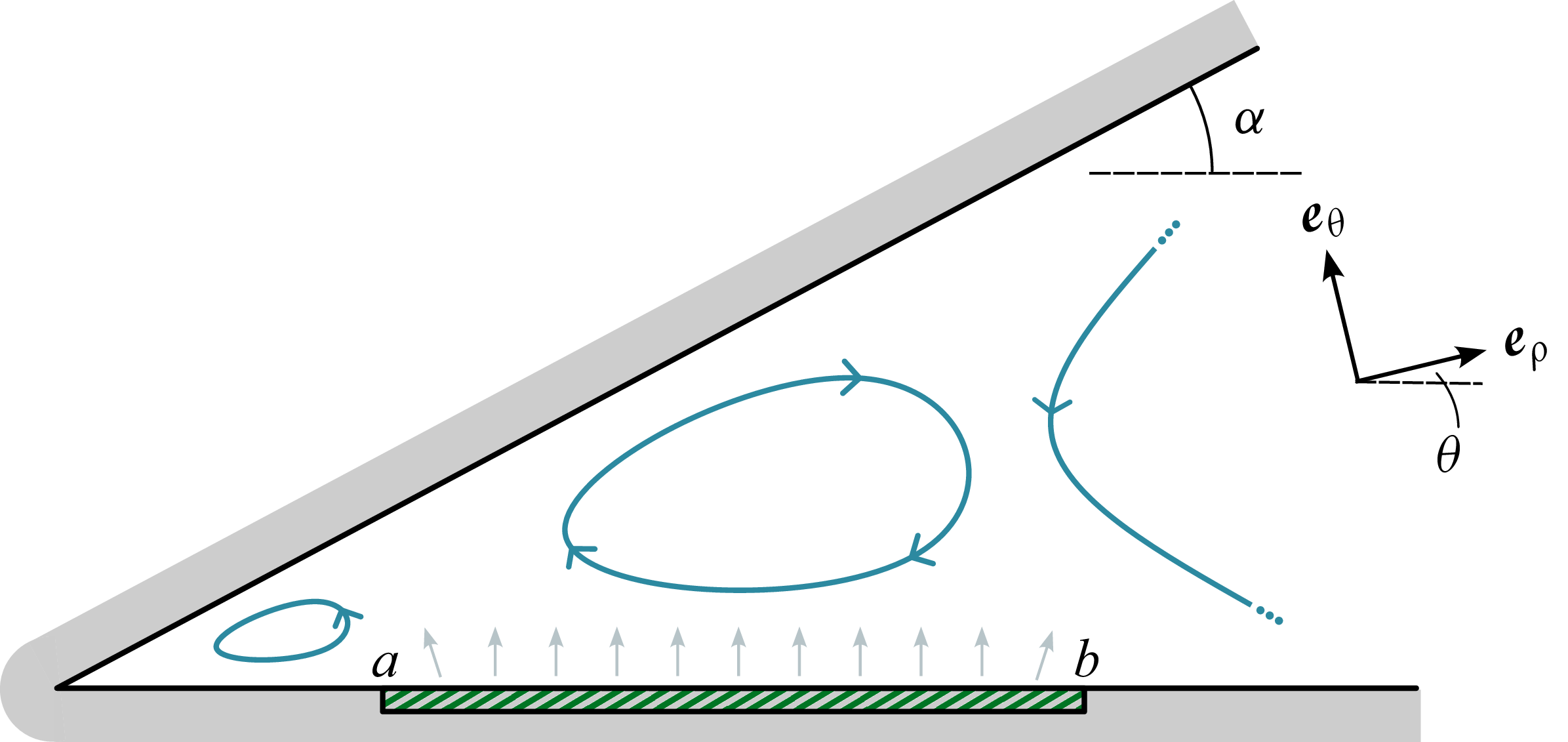


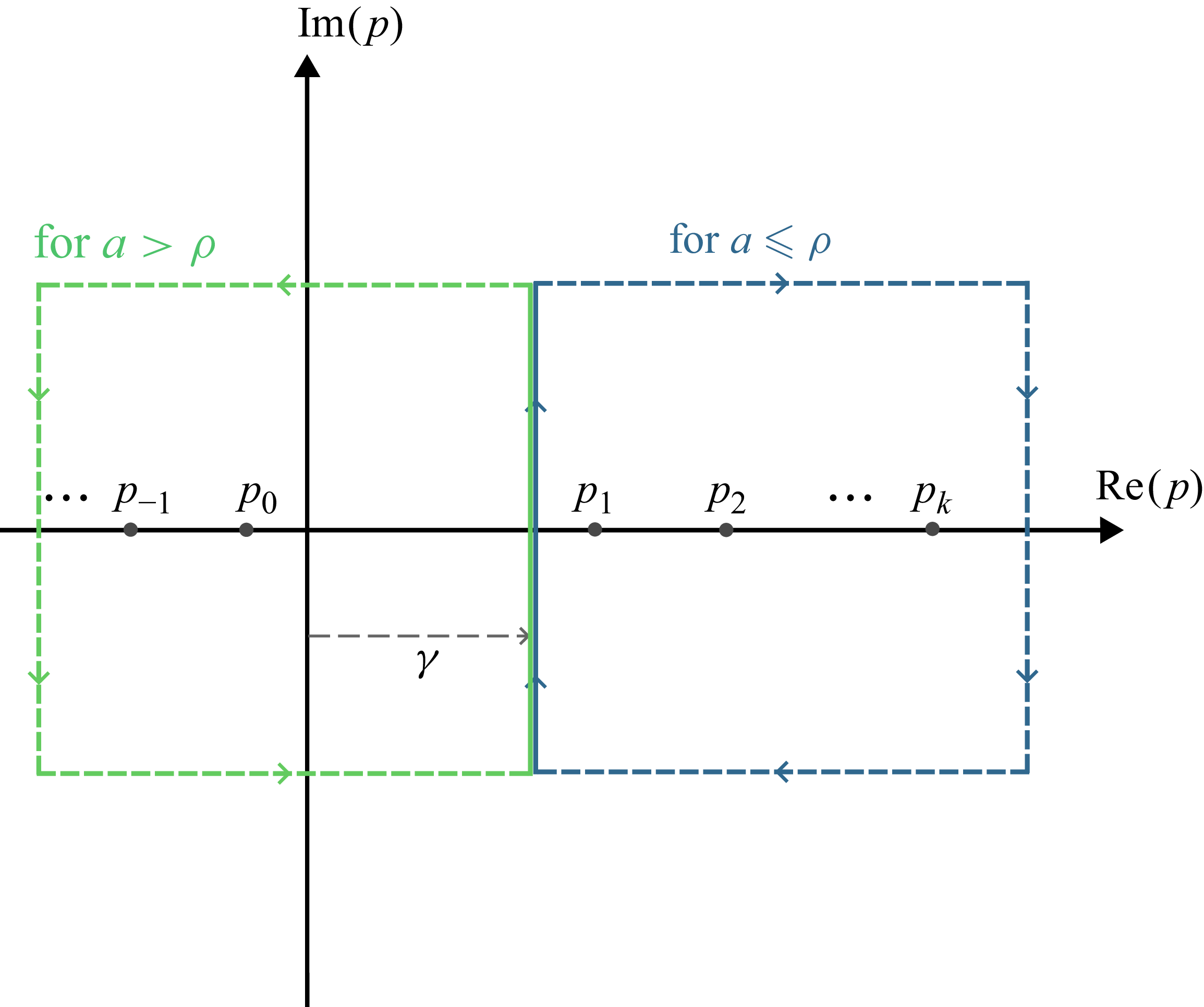


 Open access