


1. Introduction
Incentivizing experimental choices with real stakes is a key feature of experimental economics. This approach is a long-standing norm in experimental economics, as participants’ desire to optimize real-world outcomes can improve the generalizability of experimental behavior by overpowering biases known to emerge in experimental environments (see Smith, Reference Smith1976; Smith, Reference Smith1982; Roth, Reference Roth1995; Camerer and Hogarth, Reference Camerer and Hogarth1999; Hertwig and Ortmann, Reference Hertwig and Ortmann2001; Schram, Reference Schram2005; Bardsley et al., Reference Bardsley, Cubitt, Loomes, Starmer, Sugden and Moffat2009; Charness et al., Reference Charness, Gneezy and Halladay2016; Svorenčik and Maas, Reference Svorenčik and Maas2016; Clot et al., Reference Clot, Grolleau and Ibanez2018). However, this norm is starting to shift. Top economics publications are becoming increasingly open to publishing results from hypothetical-stakes experiments, and large-scale general-population surveys such as the Global Preferences Survey are now eliciting economic preferences using hypothetical-stakes experiments (e.g., see Golsteyn et al., Reference Golsteyn, Grönqvist and Lindahl2014; Cadena and Keys, Reference Cadena and Keys2015; Kuziemko et al., Reference Kuziemko, Norton, Saez and Stantcheva2015; Alesina et al., Reference Alesina, Stantcheva and Teso2018; Falk et al., Reference Falk, Becker, Dohmen, Enke, Huffman and Sunde2018; Sunde et al., Reference Sunde, Dohmen, Enke, Falk, Huffman and Meyerheim2022; Kumar et al., Reference Kumar, Gorodnichenko and Coibion2023; Stango and Zinman, Reference Stango and Zinman2023; Coibion et al., Reference Coibion, Georgarakos, Gorodnichenko, Kenny and Weber2024). Recent research also shows that some outcome variables do not statistically significantly differ on average between real-stakes and hypothetical-stakes conditions (Brañas-Garza et al., Reference Brañas-Garza, Kujal and Lenkei2019; Brañas-Garza et al., Reference Brañas-Garza, Estepa-Mohedano, Jorrat, Orozco and Rascón-Ramírez2021; Matousek, Havranek, & Irsova, Reference Matousek, Havranek and Irsova2022; Alfonso et al., Reference Alfonso, Brañas-Garza, Jorrat, Lomas, Prissé, Vasco and Vázquez-De Francisco2023; Brañas-Garza et al., Reference Brañas-Garza, Jorrat, Espín and Sánchez2023; Enke et al., Reference Enke, Gneezy, Hall, Martin, Nelidov, Offerman and van de Ven2023; Hackethal et al., Reference Hackethal, Kirchler, Laudenbach, Razen and Weber2023). Citing some of this recent hypothetical bias research (in particular Matousek, Havranek, & Irsova, Reference Matousek, Havranek and Irsova2022), the announcement for Experimental Economics’ special issue on incentivization states: “There is good rationale for incentivized experiments,but recently there has been evidence that incentivization may not always matter”.Footnote 1
This paper shows econometrically and empirically that the existing hypothetical bias literature does not statistically support omitting real stakes in most modern experiments. I begin by distinguishing two types of experiments. In ‘elicitation experiments’, no intervention is varied, and treatment effects (TEs) are not of interest. In contrast, ‘intervention experiments’ vary at least one intervention with the goal of measuring its TE. Elicitation experiments made up a large proportion of early experimental economics research, and though they remain important to this day, most modern economic experiments are intervention experiments.
Econometrically, traditional tests for hypothetical bias do not identify the hypothetical bias that matters for an intervention experiment, specifically the interaction effect between hypothetical stakes and the treatment of interest. For example, consider an intervention experiment that examines whether adding a sustainability label to a food product changes people’s willingness to pay for that product. The relevant hypothetical bias in this intervention experiment is the difference in the sustainability label’s estimated TE between hypothetical-stakes and real-stakes conditions. In a 2x2 factorial experiment that varies both the sustainability label and hypothetical versus real stakes, this difference in TE estimates can be captured by the interaction effect between a dummy indicating the sustainability label treatment group and a dummy indicating the hypothetical-stakes condition.
Most traditional hypothetical bias experiments are not factorial, only randomizing participants into either real-stakes or hypothetical-stakes conditions, eliciting an outcome, and testing whether the difference in average outcomes between the two conditions is statistically significant (e.g., Brañas-Garza et al., Reference Brañas-Garza, Kujal and Lenkei2019; Brañas-Garza et al., Reference Brañas-Garza, Estepa-Mohedano, Jorrat, Orozco and Rascón-Ramírez2021; Alfonso et al., Reference Alfonso, Brañas-Garza, Jorrat, Lomas, Prissé, Vasco and Vázquez-De Francisco2023; Brañas-Garza et al., Reference Brañas-Garza, Jorrat, Espín and Sánchez2023; Hackethal et al., Reference Hackethal, Kirchler, Laudenbach, Razen and Weber2023). For example, one could imagine a version of the experiment in the previous paragraph where willingness to pay is elicited only for the version of the food product without the sustainability label, either under hypothetical-stakes or real-stakes conditions. The only estimable TE in such an experiment is the effect of hypothetical stakes on willingness to pay. This is the average marginal effect of hypothetical stakes on the outcome.
The average marginal effect estimated in such traditional hypothetical bias experiments is a fully informative hypothetical bias measure for elicitation experiments, but it is not fully informative for intervention experiments. The average marginal effect of hypothetical stakes has no general relationship with the interaction effect between hypothetical stakes and any treatment of interest. This makes sense for two reasons. First, a researcher cannot identify an interaction effect if all the researcher knows is the average marginal effect of one of the two variables in the interaction. Second, it is unrealistic to expect hypothetical stakes to affect every possible intervention’s TE on a given outcome in the exact same way.
Empirically, TE-uninformative hypothetical bias measures often meaningfully misidentify TE-informative hypothetical biases. I re-analyze replication data from three recent hypothetical bias experiments that vary both a treatment of interest and hypothetical stakes. These experiments allow me to directly estimate the interaction effects between hypothetical stakes and treatments of interest, and to compare these interaction effects with the TE-uninformative hypothetical bias estimates typically produced in hypothetical bias experiments. I find that TE-uninformative hypothetical bias measures often yield different conclusions than TE-informative hypothetical bias measures. TE-uninformative hypothetical bias measures can even exhibit sign flips when compared to TE-informative hypothetical bias measures. That is, TE-uninformative hypothetical bias estimates are sometimes positive even when TE-informative hypothetical biases are negative (and vice versa).
These findings raise doubts about the practical value of recent advances in the hypothetical bias literature. My econometric results show that recent studies finding no statistically significant differences in certain outcomes between real-stakes and hypothetical-stakes conditions do not justify the broader conclusion that real stakes ‘do not matter’ for all TEs on those outcomes. Researchers who abandon real experimental stakes in their intervention experiments based on these findings may be misled, and TEs estimated in these experiments may be confounded by meaningful hypothetical biases. I conclude that it remains useful to maintain existing norms in experimental economics that favor incentivizing experimental choices with stakes that are real, either probabilistically or with certainty.
Section 2 provides a taxonomy of experiments that clarifies the relevant differences between elicitation experiments and intervention experiments, and establishes notation for the paper. Section 3 discusses how hypothetical bias is measured in the historical literature. Section 4 establishes econometrically why these traditional methods for measuring hypothetical bias fail to identify TE-informative hypothetical biases. Section 5 provides three empirical applications demonstrating that TE-informative and TE-uninformative hypothetical bias measures often meaningfully differ. Section 6 discusses the implications of my findings for norms in experimental economics. Section 7 concludes.
2. Terminology and Notation
I start by establishing a simple taxonomy of experiments. Let  $Y_i \in \mathbb{R}$ be the outcome variable of interest, and let
 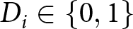 $D_i \in \left\{0, 1\right\}$ be an experimental intervention of interest. For this paper, a ‘real-stakes’ condition is one in which participants’ experimental choices map onto real-world payoffs or consequences. In contrast, ‘hypothetical-stakes’ conditions do not link experimental choices to real-world consequences.
I distinguish between two types of experiments, the first of which is an ‘elicitation experiment.’ This sort of experiment does not apply any intervention, and there are no TEs to estimate. The primary aim of an elicitation experiment is to use experimental procedures to obtain descriptive statistics concerning  $Y_i$, usually sample means or medians. For example, a researcher interested in learning the average consumer’s willingness to pay for a product may run an experiment employing the Becker-DeGroot-Marschak (Reference Becker, DeGroot and Marschak1964) procedure to obtain an incentive-compatible measure of participants’ willingness to pay. This is undoubtedly an experiment, but there is no TE to speak of; the researcher is just interested in descriptive statistics on willingness to pay. This is thus an elicitation experiment.
The second type of experiment I consider is an ‘intervention experiment.’ Unlike an elicitation experiment, an intervention experiment employs an intervention of interest  $D_i$, and the researcher is interested in the TE of this intervention. To extend the example from the previous paragraph, suppose that the researcher wants to know the effect of a specific product characteristic on willingness to pay. They could repeat the same Becker-DeGroot-Marschak experiment, but randomly assign half of the participants to consider a product with that characteristic. The researcher can then estimate the TE of that characteristic on willingness to pay by taking the difference in average willingness to pay between the two halves of the sample. This would be an intervention experiment.Footnote 2
In general, ‘hypothetical bias’ can be defined as the difference in the statistic of interest resulting from a change in stakes condition  $S_i$, which is parameterized here as a dummy variable indicating that participant
  $i$ faces real stakes with probability
  $p'$ instead of probability
  $p$. That is, for
  $p, p' \in [0, 1]$ with
  $p \neq p'$, I define
 \begin{align}
S_i = \begin{cases}
0~\text{if}~\text{participant}\ i'\text{s stakes are real with probability}\ p \\
1~\text{if}~\text{participant}\ i'\text{s stakes are real with probability}\ p'
\end{cases}.
\end{align}
\begin{align}
S_i = \begin{cases}
0~\text{if}~\text{participant}\ i'\text{s stakes are real with probability}\ p \\
1~\text{if}~\text{participant}\ i'\text{s stakes are real with probability}\ p'
\end{cases}.
\end{align} Typically,  $p = 1$ and
  $p' = 0$, meaning
  $S_i = 1$ indicates pure hypothetical stakes whereas
  $S_i = 0$ indicates pure real stakes. I use this definition of
  $S_i$ throughout the remainder of this paper for simplicity. However, this framework can be extended to examine potential biases arising from switching between any pair of probabilities that stakes are real. Because of this generalizability, the statistical framework that I introduce throughout this paper can also be used to explore hypothetical biases arising from probabilistic incentivization. I return to this point in Section 6.2. The specific bias induced by switching between stakes conditions depends on the statistic of interest.
3. Historical Measurement of Hypothetical Bias
Many early seminal contributions in experimental economics are elicitation experiments. A preponderance of economic experiments published prior to 1960 focused heavily on testing the predictions of prevailing economic theories and documenting empirical regularities observed in laboratory experiments (Roth, Reference Roth1995). This was largely done using elicitation experiments to measure various economic preferences and behaviors, including indifference curves for different bundles of goods (Thurstone, Reference Thurstone1931; Rousseas and Hart, Reference Rousseas and Hart1951), risk and ambiguity preferences (Mosteller & Nogee, Reference Mosteller and Nogee1951; Allais, Reference Allais1953), strategies in games (Flood, Reference Flood1958), and prices in experimental markets (Chamberlin, Reference Chamberlin1948). This is not to say that no intervention experiments were conducted in experimental economics’ early years, but elicitation experiments certainly played a leading role.
This historical context is important because the preponderance of elicitation experiments in experimental economics’ early years influenced the statistical parameters that experimental economists were interested in when disciplinary norms on experimental stakes first emerged. The influential ‘Wallis-Friedman critique’ of hypothetical choice menus was already published in 1942, and played a key role in prompting leading experimental economists to incentivize their experiments with real stakes (see Wallis and Friedman, Reference Wallis and Friedman1942; Svorenčik and Maas, Reference Svorenčik and Maas2016; Ortmann, Reference Ortmann2016). As a result, by the end of the 1950s, experimental economists were already predominantly incentivizing their experiments with real stakes (Roth, Reference Roth1995). The fact that experimental economists at this time were often more interested in descriptive statistics about people’s basic economic preferences than the TEs of economically-relevant interventions influenced the reasons why experimental economists cared about real stakes, as well as the ways in which they measured bias when real stakes were not provided.
Two key justifications for incentivizing experiments with real stakes emerged from this early literature, the first of which is that hypothetical stakes may affect the average preference or behavior elicited from a sample. This implies that hypothetical stakes bias the expected value of  $Y_i$. I refer to hypothetical biases on average elicited outcomes as ‘classical hypothetical bias (CHB)’, which can be written as
 \begin{align}
\text{CHB} \equiv \mathbb{E}\left[Y_i(p') - Y_i(p)\right].
\end{align}
\begin{align}
\text{CHB} \equiv \mathbb{E}\left[Y_i(p') - Y_i(p)\right].
\end{align} In other words, CHB is the average marginal effect of changes in stakes conditions on the outcome of interest. When the statistic of interest is the sample mean of  $Y_i$, CHB can be easily parameterized in a linear model of the form
 \begin{align}
Y_i = \alpha + \delta S_i + \epsilon_i.
\end{align}
\begin{align}
Y_i = \alpha + \delta S_i + \epsilon_i.
\end{align} If  $S_i$ is randomly assigned, then one can invoke unconfoundedness condition
  $\epsilon_i \perp S_i$ to examine the causal effect of hypothetical stakes in the following simple potential outcomes framework (see Rubin, Reference Rubin1974; Rubin, Reference Rubin2005):
 \begin{align}
Y_i(1) - Y_i(0) = (\alpha + \delta) - \alpha = \delta,
\end{align}
\begin{align}
Y_i(1) - Y_i(0) = (\alpha + \delta) - \alpha = \delta,
\end{align} where  $Y_i(S)$ is the potential outcome of
  $Y_i$ depending on stakes condition
  $S \in \left\{0, 1\right\}$. It then holds trivially that
 \begin{equation}\text{CHB} = \mathbb{E}\left[Y_i(1) - Y_i(0)\right] = \mathbb{E}[\delta] = \delta.
\end{equation}
\begin{equation}\text{CHB} = \mathbb{E}\left[Y_i(1) - Y_i(0)\right] = \mathbb{E}[\delta] = \delta.
\end{equation}In other words, under experimental randomization of stakes conditions and linear models commonly applied when analyzing experiments, CHB can be identified as the difference in mean outcome values between hypothetical-stakes and real-stakes conditions.
CHB is a well-documented factor in economic experiments. Camerer and Hogarth (Reference Camerer and Hogarth1999) provide systematic evidence of CHB, reviewing 36 studies that compare a hypothetical-stakes condition with a real-stakes control.Footnote 3 26 of these studies (72%) show that hypothetical stakes affect the central tendency of at least one outcome. Similarly, Harrison and Rutström (Reference Harrison and Rutström2008) review 35 studies measuring CHB in experiments on willingness to pay. Only two of these studies (5.7%) report zero CHB, and 16 studies (45.7%) report statistically significant CHB. Smith and Walker (Reference Smith and Walker1993) and Hertwig and Ortmann (Reference Hertwig and Ortmann2001) provide similar systematic evidence.
Significant CHB is found in a variety of experimental settings. These include ultimatum games (Sefton, Reference Sefton1992), public goods games (Cummings et al., Reference Cummings, Elliott, Harrison and Murphy1997), auctions (List, Reference List2001), and multiple price lists (Harrison et al., Reference Harrison, Johnson, Mcinnes and Rutström2005). CHB is particularly severe in contingent valuation experiments. Experimental participants routinely overstate their willingness to pay for public goods such as environmental services (see Hausman, Reference Hausman2012). Meta-analytic estimates of CHB in contingent valuation imply that under hypothetical stakes, people overstate their real-stakes willingness to pay by 35% (Murphy et al., Reference Murphy, Allen, Stevens and Weatherhead2005) to 200% (List, Reference List2001). Even though some recent studies find that experimental outcomes do not statistically significantly differ between hypothetical-stakes and real-stakes conditions (Brañas-Garza et al., Reference Brañas-Garza, Kujal and Lenkei2019; Brañas-Garza et al., Reference Brañas-Garza, Estepa-Mohedano, Jorrat, Orozco and Rascón-Ramírez2021; Matousek, Havranek, & Irsova, Reference Matousek, Havranek and Irsova2022; Brañas-Garza et al., Reference Brañas-Garza, Jorrat, Espín and Sánchez2023; Enke et al., Reference Enke, Gneezy, Hall, Martin, Nelidov, Offerman and van de Ven2023; Hackethal et al., Reference Hackethal, Kirchler, Laudenbach, Razen and Weber2023), a large body of literature demonstrates substantial risks of CHB in many experimental contexts.
The second rationale for incentivizing experiments with real stakes is reducing noise. Experimental economists typically believe that participants motivated by real stakes make more careful and deliberative choices than participants facing hypothetical stakes, and thus that real stakes reduce noise in experimental outcomes (see Bardsley et al., Reference Bardsley, Cubitt, Loomes, Starmer, Sugden and Moffat2009). Smith and Walker (Reference Smith and Walker1993) survey 31 hypothetical bias studies and find that in virtually all, the variance of outcomes around theory-predicted values decreases when stakes are real. Camerer and Hogarth (Reference Camerer and Hogarth1999) note nine experiments where hypothetical stakes change the variance or convergence of experimental outcomes (usually by increasing variance or decreasing convergence). Hertwig and Ortmann (Reference Hertwig and Ortmann2001) identify two additional experiments where similar effects are observed.
However, the measurement of these ‘noise reduction’ effects is not systematic and differs between studies. Some studies focus on changes in the standard deviation (SD) or variance of outcomes between stakes conditions (e.g.,Wright and Anderson, Reference Wright and Anderson1989; Ashton, Reference Ashton1990; Irwin et al., Reference Irwin, McClelland and Schulze1992; Forsythe et al., Reference Forsythe, Horowitz, Savin and Sefton1994). Others assess noise by examining deviations from some theory-predicted value, such as price deviations from a competitive market price (see Edwards, Reference Edwards1953; Smith, Reference Smith1962; Smith, Reference Smith1965; Jamal and Sunder, Reference Jamal and Sunder1991; Smith and Walker, Reference Smith and Walker1993). Furthermore, changes in variance between stakes conditions are typically not accompanied by a precision measure, such as a standard error (SE), to qualify the magnitude of these between-condition variance shifts.Footnote 4 It is thus unclear whether observed differences in outcome variances between stakes conditions reflect genuine effects or are simply artefacts of sampling variation.
I parameterize the effect of hypothetical stakes on noise as an ‘outcome SD bias (OSDB)’, which can be written as
 \begin{align}
\text{OSDB} \equiv \mathbb{E}\left[\sigma_{Y_i}(p') - \sigma_{Y_i}(p)\right].
\end{align}
\begin{align}
\text{OSDB} \equiv \mathbb{E}\left[\sigma_{Y_i}(p') - \sigma_{Y_i}(p)\right].
\end{align} A point estimate of this bias can be obtained by simply taking the difference in outcome SD  $\sigma_{Y_i}$ between stakes conditions. I define noise in this way because not all experimental outcomes have clear values that theoretically ‘should’ be observed in experimental data, whereas SDs can be used to measure noise across experimental contexts.
The SE of the OSDB can be obtained via bootstrap. Specifically, I propose to estimate the SE of OSDB by resampling the estimation sample’s observations/clusters  $B$ times with replacement. In each bootstrap sample, one can store
  $\sigma_{Y_i}(p') - \sigma_{Y_i}(p)$ as the difference in the sample standard deviations of
  $Y_i$ between the groups facing hypothetical and real stakes (respectively). After all
  $B$ bootstrap samples are obtained, one can then compute SE(OSDB) as the sample standard deviation of
  $\sigma_{Y_i}(p') - \sigma_{Y_i}(p)$ across all bootstrap samples. Another alternative approach that can be applied in a traditional hypothetical bias experiment where the only treatment varied is the stakes condition is to test differences in outcome variance between hypothetical-stakes and real-stakes groups using Levene’s test or subsequent derivations (see Gastwirth et al., Reference Gastwirth, Gel and Miao2009).
Most studies on the effects of real stakes in experiments focus exclusively on CHB and OSDB. Brañas-Garza et al. (Reference Brañas-Garza, Kujal and Lenkei2019) meta-analytically find that scores on the cognitive reflection test do not statistically significantly differ between real-stakes and hypothetical-stakes settings (though see Yechiam and Zeif, Reference Yechiam and Zeif2023). Brañas-Garza et al. (Reference Brañas-Garza, Estepa-Mohedano, Jorrat, Orozco and Rascón-Ramírez2021) use equivalence testing to show statistically significant evidence that the count of safe choices made on a Holt and Laury (Reference Holt and Laury2002) multiple price list does not differ between real-stakes and hypothetical-stakes conditions (see also Fitzgerald, Reference Fitzgerald2025). Matousek, Havranek, & Irsova (Reference Matousek, Havranek and Irsova2022) find that the meta-analytic average individual discount rate does not statistically significantly differ between real-stakes and hypothetical-stakes experiments. Brañas-Garza et al. (Reference Brañas-Garza, Jorrat, Espín and Sánchez2023) find that the means and SDs of time discounting factors are not statistically significantly different between real-stakes and hypothetical-stakes conditions, and Hackethal et al. (Reference Hackethal, Kirchler, Laudenbach, Razen and Weber2023) find that the same is true of the number of risky choices that participants make in a multiple price list experiment. Enke et al. (Reference Enke, Gneezy, Hall, Martin, Nelidov, Offerman and van de Ven2023) find no statistically significant differences in the number of correct answers on the cognitive reflection test, a base rate neglect test, or a contingent reasoning test between real-stakes and hypothetical-stakes conditions. These studies are reporting estimates of CHB, with Brañas-Garza et al. (Reference Brañas-Garza, Jorrat, Espín and Sánchez2023) and Hackethal et al. (Reference Hackethal, Kirchler, Laudenbach, Razen and Weber2023) also reporting evidence on OSDB.
Though CHB and OSDB are fully informative measures of hypothetical bias in elicitation experiments – which played early leading roles in experimental economics when norms on real stakes first emerged – most modern work in experimental economics (and experimental social sciences more broadly) is not limited to elicitation experiments. Although elicitation experiments remain important today, many researchers are now more focused on obtaining clean causal TEs from experiments than they are in simply obtaining descriptive statistics. Such experimental TEs were, and still are, crucial antecedents of the credibility revolution in economics (Angrist and Pischke, Reference Angrist and Pischke2010). However, as the next section shows, CHB and OSDB are not fully informative measures of hypothetical bias for experimental TEs.
4. Hypothetical Bias for Treatment Effects
4.1. Treatment Effect Point Estimates: IHB
CHB is not fully informative for describing hypothetical bias on TEs. In fact, Equation 3 shows that CHB can be modeled and estimated while completely ignoring intervention  $D_i$. Any statistical framework used to identify the effect of real stakes on TEs must incorporate
  $D_i$, and must allow the possibility that stakes condition
  $S_i$ can influence TEs.
My econometric framework for modeling the impact of hypothetical stakes on TEs considers a simple 2x2 factorial experiment where both treatment  $D_i$ and stakes condition
  $S_i$ are randomized with equal probability across participants. Following Guala (Reference Guala2001), I model the effects of
  $D_i$ and
  $S_i$ using a simple heterogeneous treatment effects framework:
 \begin{align}
Y_i = \alpha + \beta_1D_i + \beta_2S_i + \beta_3(D_i \times S_i) + \mu_i.
\end{align}
\begin{align}
Y_i = \alpha + \beta_1D_i + \beta_2S_i + \beta_3(D_i \times S_i) + \mu_i.
\end{align} Randomization of  $D_i$ and
  $S_i$ confers unconfoundedness:
  $\mu_i \perp \left\{D_i, S_i\right\}$. Participant
  $i$’s TE
  $\tau_i$ – the marginal effect of
  $D_i$ on
  $Y_i$ – can thus be modeled in the following potential outcomes framework:
 \begin{align}
\tau_i = Y_i(1, S) - Y_i(0, S) = \begin{cases}
\beta_1~\text{if}~S_i = 0 \\
\beta_1 + \beta_3~\text{if}~S_i = 1
\end{cases}.
\end{align}
\begin{align}
\tau_i = Y_i(1, S) - Y_i(0, S) = \begin{cases}
\beta_1~\text{if}~S_i = 0 \\
\beta_1 + \beta_3~\text{if}~S_i = 1
\end{cases}.
\end{align} Here  $Y_i(D, S)$ represents the potential outcome of
  $Y_i$ depending on intervention status
  $D \in \left\{0, 1\right\}$ and stakes condition
  $S \in \left\{0, 1\right\}$. For what follows, suppose that the statistic of interest is the average TE
  $\tau \equiv \mathbb{E}\left[\tau_i\right]$.
The hypothetical bias on the point estimate of  $\tau$ can be derived as a simple difference-in-differences, which I refer to as ‘interactive hypothetical bias (IHB)’:
 \begin{align}
\text{IHB} &\equiv \mathbb{E}\left[\tau_i\left(p'\right) - \tau_i\left(p\right)\right] \qquad\qquad\qquad\qquad\qquad\qquad\quad
\end{align}
\begin{align}
\text{IHB} &\equiv \mathbb{E}\left[\tau_i\left(p'\right) - \tau_i\left(p\right)\right] \qquad\qquad\qquad\qquad\qquad\qquad\quad
\end{align} \begin{align}
&= \mathbb{E}\left[Y_i(1, 1) - Y_i(0, 1)\right] - \mathbb{E}\left[Y_i(1, 0) - Y_i(0, 0)\right]
\end{align}
\begin{align}
&= \mathbb{E}\left[Y_i(1, 1) - Y_i(0, 1)\right] - \mathbb{E}\left[Y_i(1, 0) - Y_i(0, 0)\right]
\end{align} \begin{align}
&= (\beta_1 + \beta_3) - \beta_1 = \beta_3.\qquad\qquad\qquad\qquad\qquad
\end{align}
\begin{align}
&= (\beta_1 + \beta_3) - \beta_1 = \beta_3.\qquad\qquad\qquad\qquad\qquad
\end{align} This implies that hypothetical stakes bias the TE’s point estimate if and only if  $\beta_3 \neq 0$. This yields an intuitive conclusion: in a factorial experiment that randomizes both an intervention and hypothetical stakes, any hypothetical bias in the point estimate of the intervention’s TE is fully captured by the interaction effect between the intervention and hypothetical stakes.
IHB is a fully informative measure of hypothetical bias in intervention experiments, but CHB does not identify this term. Under the data-generating process in Equation 7, the marginal effect of  $S_i$ on
  $Y_i$ is
 \begin{align}
\delta_i = Y_i\left(D, 1\right) - Y_i\left(D, 0\right) = \begin{cases}
\beta_2~\text{if}~D_i = 0 \\
\beta_2 + \beta_3~\text{if}~D_i = 1
\end{cases}.
\end{align}
\begin{align}
\delta_i = Y_i\left(D, 1\right) - Y_i\left(D, 0\right) = \begin{cases}
\beta_2~\text{if}~D_i = 0 \\
\beta_2 + \beta_3~\text{if}~D_i = 1
\end{cases}.
\end{align} The average marginal effect of  $S_i$ on
  $Y_i$ can be defined by taking an expectation over Equation 12:
 \begin{align}
\mathbb{E}\left[\delta_i\right] = \beta_2 + \mathbb{E}\left[D_i\right]\beta_3.
\end{align}
\begin{align}
\mathbb{E}\left[\delta_i\right] = \beta_2 + \mathbb{E}\left[D_i\right]\beta_3.
\end{align} As discussed in Section 3, CHB is the average marginal effect of  $S_i$ on
  $Y_i$. This implies that
  $\text{CHB} = \beta_2 + \mathbb{E}\left[D_i\right]\beta_3$. In other words, in this 2x2 factorial experiment, CHB is a weighted average of (1) the marginal effect of hypothetical stakes on the outcome when
  $D_i = 0$ and (2) that marginal effect when
  $D_i = 1$. This weighted average does not identify IHB; it only identifies a linear combination of IHB with other parameters.
Researchers thus cannot credibly identify IHB in hypothetical bias experiments that only vary  $S_i$. Isolating IHB
  $(\beta_3)$ from the CHB parameter estimated in most hypothetical bias experiments
  $(\beta_2 + \mathbb{E}\left[D_i\right]\beta_3)$ requires the researcher to know at least two of the three following parameters:
  $\beta_2$,
  $\beta_3$, and
  $\mathbb{E}\left[D_i\right]$. However,
  $\mathbb{E}\left[D_i\right]$ is undefined in an experiment where no
  $D_i$ is varied. Additionally, the researcher cannot identify
  $\beta_3$ alone without knowing the interaction effect between
  $S_i$ and
  $D_i$, which is not estimable if no
  $D_i$ is varied. This implies that identifying IHB requires a factorial experiment that varies both intervention
  $D_i$ and stakes condition
  $S_i$ in a way that permits unconfounded estimation of these treatments’ individual and joint effects on
  $Y_i$.
Trying to infer IHB from CHB can yield misleading conclusions, including both magnitude and sign errors. By Equation 13, if  $\left|\beta_2\right|$ is large and
  $\beta_3 = 0$, then CHB will be large even though IHB is zero. Likewise, if
  $\beta_2 = -\mathbb{E}\left[D_i\right]\beta_3$, then CHB will be zero no matter how large IHB is. In a similar vein, if
  $\beta_2$ is sufficiently negative, then IHB can be positive while CHB is negative, and if
  $\beta_2$ is sufficiently positive, then IHB can be negative while CHB is positive. In fact, CHB and IHB almost always differ.
Proposition 4.1. Whenever  $\beta_3 \neq \frac{\beta_2}{1 - \mathbb{E}\left[D_i\right]}$, CHB and IHB differ.
 \begin{align*}
\beta_3 &\neq \frac{\beta_2}{1 - \mathbb{E}\left[D_i\right]} \\
\beta_3 &\neq \beta_2 + \mathbb{E}\left[D_i\right]\beta_3 \\
\mathbb{E}\left[Y_i(1, 1) - Y_i(0, 1)\right] - \mathbb{E}\left[Y_i(1, 0) - Y_i(0, 0)\right]
&\neq \mathbb{E}\left[Y_i(D, 1) - Y_i(D, 0)\right] \quad \text{(Equations 9-13)} \\
\text{IHB} &\neq \text{CHB} \quad \text{(Equations 5 and 10)}
\end{align*}
\begin{align*}
\beta_3 &\neq \frac{\beta_2}{1 - \mathbb{E}\left[D_i\right]} \\
\beta_3 &\neq \beta_2 + \mathbb{E}\left[D_i\right]\beta_3 \\
\mathbb{E}\left[Y_i(1, 1) - Y_i(0, 1)\right] - \mathbb{E}\left[Y_i(1, 0) - Y_i(0, 0)\right]
&\neq \mathbb{E}\left[Y_i(D, 1) - Y_i(D, 0)\right] \quad \text{(Equations 9-13)} \\
\text{IHB} &\neq \text{CHB} \quad \text{(Equations 5 and 10)}
\end{align*}□
The sufficient condition in Proposition 4.1 holds almost always, as the interaction effect between an intervention and some moderator is virtually never exactly the same as the average marginal effect of the moderator itself.
Recent research on hypothetical bias in experiments – which focuses almost exclusively on CHB – must be understood in this context. Though Brañas-Garza et al. (Reference Brañas-Garza, Kujal and Lenkei2019), Matousek, Havranek, & Irsova (Reference Matousek, Havranek and Irsova2022), Brañas-Garza et al. (Reference Brañas-Garza, Jorrat, Espín and Sánchez2023), and Hackethal et al. (Reference Hackethal, Kirchler, Laudenbach, Razen and Weber2023) respectively find no statistically significant CHBs on cognitive reflection test scores, discount rates, time preferences, and risk preferences, this does not imply that hypothetical stakes induce zero bias for any intervention TEs on these outcomes. Further, for a given outcome variable, there is no ‘one true’ IHB for all interventions, as different interventions likely exhibit different IHBs for the same outcome.
4.2. Treatment Effect Standard Errors: TESEB
Hypothetical bias on TE SEs can be identified in a similar fashion to hypothetical bias on TE point estimates. I parameterize hypothetical bias on TE precision as ‘TE SE bias (TESEB)’:
 \begin{align}
\text{TESEB} &\equiv \mathbb{E}\left[\text{SE}\left(\tau\left(p'\right)\right) - \text{SE}\left(\tau\left(p\right)\right)\right].
\end{align}
\begin{align}
\text{TESEB} &\equiv \mathbb{E}\left[\text{SE}\left(\tau\left(p'\right)\right) - \text{SE}\left(\tau\left(p\right)\right)\right].
\end{align} In practice, point estimates for TESEBs can be obtained by taking the differences in TE SEs between stakes conditions. SEs for TESEB point estimates can be estimated via bootstrapping. I propose to use a bootstrap procedure akin to that proposed for estimating the SE of OSDB (see Section 3), resampling the estimation sample’s observations/clusters  $B$ times with replacement. In each bootstrap sample, one can obtain TE SE estimates
  $\text{SE} {({\tau}{(p')})}$ and
  $\text{SE} {({\tau}{(p)})}$ in the subsamples of observations facing hypothetical and real stakes (respectively), storing the difference between them,
  $\text{SE} {({\tau}{(p')})}$ - $\text {SE}{({\tau}{(p)})}$. After all
  $B$ bootstrap samples are obtained, one can then calculate SE(TESEB) as the sample standard deviation of
  $\text{SE} {({\tau}{(p')})}$ - $\text{SE} {({\tau}{(p)})}$ across all bootstrap samples.
OSDB does not identify hypothetical biases on TE precision. The best way to show this is through a simple counterexample where OSDB and TESEB have opposite signs. Figure 1 displays data points from two simulated datasets, each of which contain 20 observations. In both datasets, the simulated intervention is assigned such that  $D_i = 0$ for
  $i \in \left\{1, 2, \cdots 10\right\}$ and
  $D_i = 1$ for
  $i \in \left\{11, 12, \cdots 20\right\}$. The first dataset arises from the data-generating process
 \begin{align}
Y_i = \begin{cases}
0.05 + 0.1(i - 1)~\text{if}~i \in \left\{1, 2, \cdots 10\right\}~(D_i = 0) \\
-0.05 + 0.15(i - 10)~\text{if}~i \in \left\{11, 12, \cdots 20\right\}~(D_i = 1)
\end{cases},
\end{align}
\begin{align}
Y_i = \begin{cases}
0.05 + 0.1(i - 1)~\text{if}~i \in \left\{1, 2, \cdots 10\right\}~(D_i = 0) \\
-0.05 + 0.15(i - 10)~\text{if}~i \in \left\{11, 12, \cdots 20\right\}~(D_i = 1)
\end{cases},
\end{align}
Figure 1. An example where OSDB and TESEB hold opposite signs
and the second dataset is constructed using the data-generating process
 \begin{align}
Y_i = \begin{cases}
0.05 + 0.1(i - 1)~\text{if}~i \in \left\{1, 2, \cdots 10\right\}~(D_i = 0) \\
1.05 + 0.1(i - 11)~\text{if}~i \in \left\{11, 12, \cdots 20\right\}~(D_i = 1)
\end{cases}.
\end{align}
\begin{align}
Y_i = \begin{cases}
0.05 + 0.1(i - 1)~\text{if}~i \in \left\{1, 2, \cdots 10\right\}~(D_i = 0) \\
1.05 + 0.1(i - 11)~\text{if}~i \in \left\{11, 12, \cdots 20\right\}~(D_i = 1)
\end{cases}.
\end{align} For purposes of exposition, suppose that these two simulated datasets represent two halves of an experimental dataset where  $D_i$ and
  $S_i$ are both randomized. Let the first half of the dataset (generated by the process in Equation 15) belong to a real-stakes sample (i.e.,
  $S_i = 0$), and let the second half of the dataset (generated by the process in Equation 16) belong to a hypothetical-stakes sample (i.e.,
  $S_i = 1$). It is clearly visible from Figure 1 that the outcome SD for the hypothetical-stakes sample (0.592) is higher than that in the real-stakes sample (0.401), so OSDB is positive. However, the TE SE from a simple linear regression model of
  $Y_i$ on
  $D_i$ is smaller in the hypothetical-stakes sample (0.135) than in the real-stakes sample (0.173), so TESEB is negative.Footnote 5 This example demonstrates that OSDB does not identify TESEB, and that interpreting OSDB estimates as evidence of how hypothetical stakes affect ‘noise’ in TE estimates can yield misleading conclusions.
To provide an intuitive example where OSDB and TESEB may take opposite signs, consider a 2x2 dictator game experiment where two treatments are varied: hypothetical vs. real stakes and gain vs. loss framing of endowment splits (e.g., see Ceccato et al., Reference Ceccato, Kettner, Kudielka, Schwieren and Voss2018). Suppose that hypothetical stakes induce inattentive dictators to anchor on endowment splits prescribed by social norms, such as the well-documented 50-50 norm (see Andreoni and Bernheim, Reference Andreoni and Bernheim2009). Such concentration of endowment splits amongst inattentive dictators would cause the SD of endowment splits across all dictators facing hypothetical stakes to decline, implying that hypothetical stakes likely yield negative OSDB. Suppose that loss framing decreases the endowment split offered by dictators. Further, suppose that no dictator anchors on a 50-50 split in the real-stakes condition, but that inattentive dictators anchor on a 50-50 split in the hypothetical-stakes condition. Then though the outcome SD is likely lower in the hypothetical-stakes condition, the TE SE would likely be higher. This is because, as presupposed, all dictators in the real-stakes condition uniformly give less to recipients when facing loss framing. However, hypothetical stakes induce TE heterogeneity; the TE for inattentive dictators is effectively zero because they continue to anchor on the 50-50 split. These conditions would imply that hypothetical stakes yield negative OSDB, but positive TESEB.
4.3. Meta-Analytic Approaches
One approach that hypothetical bias researchers sometimes use to directly estimate IHB is meta-analytically comparing TEs from studies with and without real stakes. For instance, Li et al. (Reference Li, Maniadis and Sedikides2021) conduct a meta-analysis of studies investigating anchoring effects on willingness to pay/accept. They find no statistically significant differences between the anchoring effects observed in studies with and without real stakes, and therefore conclude that real stakes have no discernible impact on anchoring effects. A similar approach could be used to estimate TESEBs by comparing meta-analytic averages of TE SEs under different stakes conditions, though Li et al. (Reference Li, Maniadis and Sedikides2021) do not make this comparison.
Meta-analyses like this do not provide clean causal estimates of the impact of real stakes, as the choice to incentivize an experiment with real stakes is endogenous. In Equation 11, the identification of IHB as a simple interaction effect between treatment  $D_i$ and stakes condition
  $S_i$ relies on a joint unconfoundedness assumption over both the treatment and the stakes condition,
  $\mu_i \perp \left\{D_i, S_i\right\}$. This is readily achieved within a factorial experiment when both the intervention and hypothetical stakes are randomly assigned. However, this unconfoundedness condition is not generally satisfied when comparing TEs across experiments, as experimental stakes conditions are typically not randomly assigned, and are likely correlated with other factors that simultaneously influence TEs and their SEs.
One important factor that likely confounds meta-analytic IHB estimates is academic disciplines. Naturally, some disciplines are more likely to provide real experimental stakes than others, and these disciplines meaningfully differ on various important dimensions, including participant pools and procedural norms in experimentation (see Hertwig and Ortmann, Reference Hertwig and Ortmann2001; Bardsley et al., Reference Bardsley, Cubitt, Loomes, Starmer, Sugden and Moffat2009). To fix a simple example, consider a meta-analytic dataset where all experiments employing real stakes are run by economists, whereas all experiments employing hypothetical stakes are run by psychologists. Further, suppose that the economics experiments recruit economics students, whereas the psychology experiments recruit psychology students. In order to credibly interpret the difference in TEs between these groups of experiments as a causal effect of hypothetical stakes, one must be willing to assume (among other things) that economics students respond to treatment in the exact same way as psychology students. However, this assumption is untenable; the same treatment can affect economics students and psychology students in significantly different ways (Van Lange et al., Reference Van Lange, Schippers and Balliet2011; van Andel et al., Reference van Andel, Tybur and Van Lange2016). Therefore, meta-analytic differences between TEs do not generally provide clean identification of IHBs. For similar reasons, meta-analytic differences between TE SEs do not generally provide clean identification of TESEBs.
4.4. Hypothetical Bias on Non-Causal Parameters
Though the discussion so far primarily focuses on causal TEs from intervention experiments, it is also inappropriate to use CHB estimates to infer conclusions about hypothetical bias on non-causal parameters such as correlations or group differences. Elicitation experiments are seldom carried out solely to obtain a single measure for a single group. Many elicitation experiments are carried out to estimate correlations between different measures or group differences in a single measure. Though such correlations and group differences are not causal parameters, the same general critique discussed throughout this paper applies: one cannot infer conclusions about hypothetical bias on correlations or group differences solely from estimates of hypothetical bias on outcome levels.
For a concrete example, consider Finocchiar Castro, Guccio, & Romeo (Reference Finocchiaro Castro, Guccio and Romeo2025),which cites insignificant CHB estimates from Brañas-Garza et al. (Reference Brañas-Garza, Estepa-Mohedano, Jorrat, Orozco and Rascón-Ramírez2021) as partial justification to use hypothetical-stakes elicitation experiments to elicit risk aversion from physicians and students. This is not an intervention experiment, as the status of an individual as a physician or a student is not exogenously varied by the research team. However, like many elicitation experiments, the paper is focused on group differences in an experimentally-elicited outcome; a headline conclusion of the paper is that physicians are less risk-averse in the monetary domain than students. This is not a causal TE, as the question of whether someone is a doctor or a student is almost certainly confounded with other personal characteristics. However, even though the paper is not focused on estimating a causal TE, it is still incorrect to interpret insignificant CHB estimates as evidence that hypothetical stakes will have negligible impacts on the estimated difference between physicians’ and students’ risk aversion. This is because hypothetical stakes could have different effects on risk aversion for physicians than for students. If hypothetical stakes do not have identical effects on risk aversion for both physicians and students, then hypothetical biase could cause the estimated risk aversion gap between physicians and students to expand, attenuate, or flip signs. The same general critique extends to correlations between continuous measures, which are increasingly analyzed in studies that seek to analyze experimentally-elicited measures as correlates or determinants of economic outcomes (e.g., see Sunde et al., Reference Sunde, Dohmen, Enke, Falk, Huffman and Meyerheim2022; Stango and Zinman, Reference Stango and Zinman2023).
5. Empirical Applications
To see whether TE-uninformative hypothetical bias measures misidentify TE-informative hypothetical biases in practice, I re-analyze data from three hypothetical bias experiments that allow for direct estimation of CHB, IHB, OSDB, and TESEB.Footnote 6 These studies have publicly available replication data and use factorial designs that simultaneously manipulate both hypothetical stakes and another intervention.
Finding experiments that satisfy these criteria is challenging. Most hypothetical bias experiments only vary stakes conditions without additional interventions (e.g., see Walker & Smith 1993; Camerer and Hogarth, Reference Camerer and Hogarth1999; Hertwig and Ortmann, Reference Hertwig and Ortmann2001; Harrison and Rutström, Reference Harrison and Rutström2008; Brañas-Garza et al., Reference Brañas-Garza, Estepa-Mohedano, Jorrat, Orozco and Rascón-Ramírez2021; Brañas-Garza et al., Reference Brañas-Garza, Jorrat, Espín and Sánchez2023; Hackethal et al., Reference Hackethal, Kirchler, Laudenbach, Razen and Weber2023). This makes it impossible to obtain IHB or TESEB estimates in these studies (see Sections 4.1 and 4.2). Even when experiments vary both an intervention and hypothetical stakes, interaction effects between these treatments are rarely reported. This is likely due to publication bias against null results (see Fanelli, Reference Fanelli2012; Franco et al., Reference Franco, Malhotra and Simonovits2014; Andrews and Kasy, Reference Andrews and Kasy2019; Chopra et al., Reference Chopra, Haaland, Roth and Stegmann2024). Interaction effects such as IHBs are notoriously noisy and difficult to sufficiently power (Muralidharan et al., Reference Muralidharan, Romero and Wüthrich2025). Many IHB estimates are thus likely statistically insignificant, meaning that many likely go unreported. Estimating IHB and TESEB in suitable studies that do not report estimates of these biases requires replication data. However, virtually no published articles provide full data and code unless their journal mandates data-sharing, many data-sharing policies are fairly recent, and many journals still do not mandate data-sharing (Askarov et al., Reference Askarov, Doucouliagos, Doucouliagos and Stanley2023; Brodeur et al., Reference Brodeur, Cook and Neisser2024).
The results of my three empirical analyses are visualized in Figure 2 and presented in detail in Table 1. For each experiment, I provide an overview of the experimental setup, explain how CHB, IHB, OSDB, and TESEB are computed, discuss how my results show that TE-uninformative hypothetical bias measures often misidentify TE-informative hypothetical bias measures.

Figure 2. Empirical results
Table 1. Detailed estimates of hypothetical bias measures

Note: CHB denotes ‘classical hypothetical bias’, IHB represents ‘interactive hypothetical bias’, OSDB denotes ‘outcome standard deviation bias’, TESEB denotes ‘TE SE bias’, and  $N$ is the effective sample size. SEs are presented in parentheses. OSDB and TESEB SEs are estimated from 10,000 (cluster) bootstrap replications.
5.1. Ceccato et al. (Reference Ceccato, Kettner, Kudielka, Schwieren and Voss2018)
Ceccato et al. (Reference Ceccato, Kettner, Kudielka, Schwieren and Voss2018, “Social Preferences Under Chronic Stress”) conduct an experiment in which participants play double-anonymous dictator games. Participants are randomly assigned either to a real-stakes room or to a hypothetical-stakes room. Once assigned to a room, participants are randomly seated. Dictators face two envelopes, one titled “Your Personal Envelope” and the other titled “Other Participant’s Envelope”. Dictators must allocate a five-euro endowment between these two envelopes. Dictators can receive a seat with ‘give’ framing, where the endowment is initially stored in “Your Personal Envelope”, or a seat with ‘take’ framing, where the endowment is initially stored in “Other Participant’s Envelope”. The experiment also takes steps to manipulate the gender of the dictator and the passive player, but for the purposes of this replication, I focus exclusively on the effect of the ‘give’ framing treatment (compared to the ‘take’ framing control) on dictator transfers. Replication data for the experiment reported in Ceccato et al. (Reference Ceccato, Kettner, Kudielka, Schwieren and Voss2018) is provided by Schwieren et al. (Reference Schwieren, Ceccato, Kettner, Kudielka and Voss2018).
For this experiment, I first estimate IHB in an ordinary least squares model of the form
 \begin{align}
\%\text{Trans}_i = \alpha + \beta_1\text{Give}_i + \beta_2S_i + \beta_3\text{Give}_iS_i + \mu_i.
\end{align}
\begin{align}
\%\text{Trans}_i = \alpha + \beta_1\text{Give}_i + \beta_2S_i + \beta_3\text{Give}_iS_i + \mu_i.
\end{align}  $\%\text{Trans}_i$ is the proportion of the endowment transferred by dictator
  $i$ (in percentage points),
  $\text{Give}_i$ indicates that dictator
  $i$ faces the ‘give’ framing treatment,
  $S_i$ indicates that dictator
  $i$ is assigned to a hypothetical-stakes room, and
  $\beta_3$ is the IHB estimate of interest. From this model, I compute CHB using the avg_slopes() command in the marginaleffects R package to obtain the average marginal effect of
  $S_i$ on
  $\%\text{Trans}_i$ (see Arel-Bundock et al., Reference Arel-Bundock, Greifer and Heiss2024). SEs for both CHB and IHB are computed using the HC3 heteroskedasticity-consistent variance-covariance estimator (see Hayes and Cai, Reference Hayes and Cai2007).
I obtain a point estimate of OSDB by simply subtracting the within-sample SD of  $\%\text{Trans}_i$ for dictators assigned to real-stakes rooms from that same SD for dictators assigned to hypothetical-stakes rooms. I then run ordinary least squares models of the form
 \begin{align}
\%\text{Trans}_i = \alpha_H + \tau_H\text{Give}_i + \mu_i, S_i = 1
\end{align}
\begin{align}
\%\text{Trans}_i = \alpha_H + \tau_H\text{Give}_i + \mu_i, S_i = 1
\end{align} \begin{align}
\%\text{Trans}_i = \alpha_R + \tau_R\text{Give}_i + \mu_i, S_i = 0.
\end{align}
\begin{align}
\%\text{Trans}_i = \alpha_R + \tau_R\text{Give}_i + \mu_i, S_i = 0.
\end{align} That is, I separately regress  $\%\text{Trans}_i$ on
  $\text{Give}_i$ for the dictators facing hypothetical and real stakes (respectively). My TESEB point estimate is simply
  $\text{SE}(\hat{\tau}_H) - \text{SE}(\hat{\tau}_R)$. To obtain SEs for both OSDB and TESEB, I repeat my procedures for obtaining OSDB and TESEB point estimates on 10,000 bootstrap resamplings of dictators. My SE estimates for OSDB and TESEB are respectively the SDs of the OSDBs and TESEBs from my bootstrap sample.
Table 1 shows that in Ceccato et al. (Reference Ceccato, Kettner, Kudielka, Schwieren and Voss2018), CHB and IHB exhibit opposite signs. CHB is significantly positive: hypothetical stakes cause dictators to transfer over nine percentage points more of their endowment to recipients. This is intuitive, as people tend to overstate their generosity when stakes are not real (e.g., see Sefton, Reference Sefton1992). However, the IHB for the impact of ‘give’ framing on endowment transfers is negative, and is even larger in magnitude than the CHB on endowment transfers (though this IHB is quite imprecise). OSDB and TESEB are both positive in this experiment, implying that hypothetical-stakes conditions exhibit more noise both for outcomes and for TEs in Ceccato et al. (Reference Ceccato, Kettner, Kudielka, Schwieren and Voss2018). However, neither OSDB nor TESEB are statistically significantly different from zero in this experiment.
5.2. Fang et al. (Reference Fang, Nayga, West, Bazzani, Yang, Lok, Levy and Snell2021)
Fang et al. (Reference Fang, Nayga, West, Bazzani, Yang, Lok, Levy and Snell2021, “On the Use of Virtual Reality in Mitigating Hypothetical Bias in Choice Experiments”) examine whether virtual reality marketplaces can reduce hypothetical bias in choice experiments. Participants choose between purchasing an original strawberry yogurt, a light strawberry yogurt, or neither product. Participants are randomized into one of five between-participant conditions. The first is a hypothetical-stakes condition where participants make product choices based on photos of the products. In the second and third conditions, participants choose between the products based on nutritional labels, with one condition employing hypothetical stakes and the other using real stakes. In the fourth and fifth conditions, participants make product decisions in a virtual reality supermarket. Stakes are real in one of these two virtual reality conditions whereas stakes are hypothetical in the other. Real stakes imply that if a participant chooses to purchase a yogurt product, then the participant commits to actually pay real money for the product, and in exchange receives the actual yogurt product. Once randomized to a condition, each participant makes purchase decisions four times, each time facing a different price menu.
Because it is the primary target of the Fang et al. (Reference Fang, Nayga, West, Bazzani, Yang, Lok, Levy and Snell2021) experiment, I focus on the effect of virtual reality on the decision to purchase. I estimate IHB in a panel data random effects model of the form
 \begin{align}
\text{Buy}_{i, p} = \alpha + \beta_1\text{VR}_i + \beta_2S_i + \beta_3\text{VR}_iS_i + \mu_{i, p},
\end{align}
\begin{align}
\text{Buy}_{i, p} = \alpha + \beta_1\text{VR}_i + \beta_2S_i + \beta_3\text{VR}_iS_i + \mu_{i, p},
\end{align} where  $i$ indexes the participant and
  $p$ indexes the price menu. I code
  $\text{Buy}_{i, p}$ as a dummy indicating that participant
  $i$ chooses to purchase either the original or light yogurt when facing price menu
  $p$,
$p$,  $\text{VR}_i$ as a dummy indicating that participant
  $i$ faces one of the two virtual reality treatments, and
  $S_i$ as a dummy indicating that participant
  $i$ is facing one of the three conditions with hypothetical stakes. As in my re-analysis of Ceccato et al. (Reference Ceccato, Kettner, Kudielka, Schwieren and Voss2018),
  $\beta_3$ is the IHB parameter of interest, and I compute CHB using the avg_slopes() command in the marginaleffects R suite to obtain the average marginal effect of
  $S_i$ on
  $\text{Buy}_{i, p}$. SEs for both IHB and CHB are clustered at the participant level.
As in my re-analysis of Ceccato et al. (Reference Ceccato, Kettner, Kudielka, Schwieren and Voss2018), I obtain a point estimate of OSDB by subtracting the SD of  $\text{Buy}_{i, p}$ for the sample facing real-stakes conditions from that same SD for the sample facing hypothetical-stakes conditions. I run random effects panel data models of the form
 \begin{align}
\text{Buy}_{i, p} &= \alpha_H + \tau_H\text{VR}_i + \mu_{i, p},~S_i = 1
\end{align}
\begin{align}
\text{Buy}_{i, p} &= \alpha_H + \tau_H\text{VR}_i + \mu_{i, p},~S_i = 1
\end{align} \begin{align}
\text{Buy}_{i, p} &= \alpha_R + \tau_R\text{VR}_i + \mu_{i, p},~S_i = 0
\end{align}
\begin{align}
\text{Buy}_{i, p} &= \alpha_R + \tau_R\text{VR}_i + \mu_{i, p},~S_i = 0
\end{align} and compute the TESEB point estimate as  $\text{SE}(\hat{\tau}_H) - \text{SE}(\hat{\tau}_R)$. To estimate SEs for OSDB and TESEB, I repeat the procedures to obtain point estimates for OSDB and TESEB in 10,000 cluster bootstrap samples (where participants
  $i$, instead of rows
  $\left\{i, p\right\}$, are resampled with replacement). I respectively compute the SEs of OSDB and TESEB as the SDs of the OSDB and TESEB point estimates in my bootstrap sample.
Table 1 shows that TE-uninformative hypothetical bias measures are markedly different from TE-informative hypothetical bias measures in Fang et al. (Reference Fang, Nayga, West, Bazzani, Yang, Lok, Levy and Snell2021). CHB is significantly positive in this experiment: hypothetical stakes increase participants’ likelihood of choosing to purchase one of the two yogurts by 18 percentage points. This reflects the intuitive and well-documented fact that people often overstate their willingness to pay when stakes are hypothetical (see List, Reference List2001; Murphy et al., Reference Murphy, Allen, Stevens and Weatherhead2005; Harrison and Rutström, Reference Harrison and Rutström2008; Hausman, Reference Hausman2012). However, the IHB estimate in this experiment is less than one third the size of the CHB estimate, and is not statistically significantly different from zero. That said, the IHB and CHB estimates are not statistically significantly different from one another.
OSDB and TESEB are both significantly negative in this experiment, but are also significantly different from each other. Hypothetical stakes significantly decrease the dispersion of purchase decisions, decreasing the SD of  $\text{Buy}_{i, p}$ by over 16 percentage points. Hypothetical stakes also statistically significantly decrease the SE of virtual reality’s TE on purchase probability, but only by 2.7 percentage points. The TESEB estimate is therefore 83.5% smaller than the OSDB estimate, and the 13.6 percentage point difference between the two bias estimates is highly significant (SE
  $=$ 2.6 percentage points).Footnote 7 These findings are additionally interesting because the fact that both OSDB and TESEB are negative in this experiment provides evidence against experimental economists’ traditional notion that real stakes typically reduce noise in experimental outcomes and TEs (see Bardsley et al., Reference Bardsley, Cubitt, Loomes, Starmer, Sugden and Moffat2009).
5.3. Enke et al. (Reference Enke, Gneezy, Hall, Martin, Nelidov, Offerman and van de Ven2023)
Enke et al. (Reference Enke, Gneezy, Hall, Martin, Nelidov, Offerman and van de Ven2023, “Cognitive Biases: Mistakes or Missing Stakes?”) investigate hypothetical biases for a variety of commonly-elicited experimental outcomes. Participants first complete two out of four possible tasks without any real stakes at play. Participants are then randomized in between-participants fashion to either a low-stakes or high-stakes condition where stakes are real to repeat these same two tasks.Footnote 8 For three of the four tasks, no interventions are implemented.Footnote 9 For these three tasks, it is not possible to estimate IHB or TESEB. However, Enke et al. (Reference Enke, Gneezy, Hall, Martin, Nelidov, Offerman and van de Ven2023) also examine the impact of stakes in an anchoring context, where there is a clear TE to examine (i.e., the anchoring effect). It is thus possible to estimate IHB and TESEB in the anchoring task.
Participants facing the anchoring task in Enke et al. (Reference Enke, Gneezy, Hall, Martin, Nelidov, Offerman and van de Ven2023) must answer two of four randomly-assigned numerical questions whose answers range from 0-100.Footnote 10 Each participant receives an anchor, constructed using the first two digits of their birth year and the last digit of their phone number. For each anchoring question, participants are first asked whether the numerical answer to the question is greater than or less than their anchor, and thereafter must provide an exact numerical answer to the question. The first anchoring question is answered with no real stakes at play. The second anchoring question is answered for (probabilistically) real stakes: participants can earn a monetary bonus if their answer to the question is within two points of the correct answer.Footnote 11 My replication of Enke et al. (Reference Enke, Gneezy, Hall, Martin, Nelidov, Offerman and van de Ven2023) focuses only on the sample facing the anchoring task. To get as close as possible to examining extensive-margin effects of real versus hypothetical stakes, I exclude participants subjected to the high-stakes treatment. Replication data for Enke et al. (Reference Enke, Gneezy, Hall, Martin, Nelidov, Offerman and van de Ven2023) is provided by Enke et al. (Reference Enke, Gneezy, Hall, Martin, Nelidov, Offerman and van de Ven2021).
Estimation procedures for Enke et al. (Reference Enke, Gneezy, Hall, Martin, Nelidov, Offerman and van de Ven2023) closely mirror those for Fang et al. (Reference Fang, Nayga, West, Bazzani, Yang, Lok, Levy and Snell2021). IHB is computed in a panel data random effects model of the form
 \begin{align}
\text{Answer}_{i, c} &= \alpha + \beta_1\text{Anchor}_{i} + \beta_2S_c + \beta_3\text{Anchor}_{i}S_c + \mu_{i, c},
\end{align}
\begin{align}
\text{Answer}_{i, c} &= \alpha + \beta_1\text{Anchor}_{i} + \beta_2S_c + \beta_3\text{Anchor}_{i}S_c + \mu_{i, c},
\end{align} where  $i$ indexes the participant and
  $c$ indexes the stakes condition.
  $\text{Anchor}_{i}$ is participant
  $i$’s anchor and
  $S_c$ is a dummy indicating that the participant is answering the first anchoring question, where there are no real stakes. After estimating this model, I use the avg_slopes() command in the marginaleffects R suite to compute CHB as the average marginal effect of
  $S_c$ on
  $\text{Answer}_{i, c}$. SEs for both IHB and CHB are clustered at the participant level.
I compute the OSDB point estimate by subtracting the SD of numerical answers to questions faced without real stakes from the same SD for questions faced when real stakes are at play. I then run random effects panel data models of the form
 \begin{align}
\text{Answer}_{i, c} &= \alpha_H + \tau_H\text{Anchor}_{i} + \mu_{i, c},~S_c = 1
\end{align}
\begin{align}
\text{Answer}_{i, c} &= \alpha_H + \tau_H\text{Anchor}_{i} + \mu_{i, c},~S_c = 1
\end{align} \begin{align}
\text{Answer}_{i, c} &= \alpha_R + \tau_R\text{Anchor}_{i} + \mu_{i, c},~S_c = 0
\end{align}
\begin{align}
\text{Answer}_{i, c} &= \alpha_R + \tau_R\text{Anchor}_{i} + \mu_{i, c},~S_c = 0
\end{align} and obtain TESEB point estimate  $\text{SE}(\hat{\tau}_H) - \text{SE}(\hat{\tau}_R)$. As in my re-analysis of Fang et al. (Reference Fang, Nayga, West, Bazzani, Yang, Lok, Levy and Snell2021), I then re-estimate the OSDB and TESEB point estimates in 10,000 cluster bootstrap samples. SEs of OSDB and TESEB are respectively computed as the SDs of the OSDB and TESEB point estimates in the bootstrap sample.
My replication of Enke et al. (Reference Enke, Gneezy, Hall, Martin, Nelidov, Offerman and van de Ven2023) shows that TE-uninformative hypothetical bias measures can misidentify TE-informative hypothetical bias not just in terms of qualitative conclusions, but also in scale. The CHB estimate is significantly positive: participants appear to offer numerical answers roughly six points higher (out of 100) when stakes are hypothetical. However, the IHB estimate is 99.7% smaller than the CHB estimate, and is not statistically significantly different from zero. Similarly, the TESEB estimate is 99.8% smaller than the OSDB estimate, though neither the OSDB estimate nor the TESEB estimate is statistically significantly different from zero.
These differences in magnitude partially reflect the fact that hypothetical stakes and interventions of interest can take on completely different scales. Considering the case of Enke et al. (Reference Enke, Gneezy, Hall, Martin, Nelidov, Offerman and van de Ven2023), it makes sense that a one-point increase in a 0-100 numerical anchor will have a relatively small impact on numerical answers compared to a binary switch from real-stakes to hypothetical-stakes conditions. Similar scale differences may emerge between TE-informative and TE-uninformative hypothetical bias measures in many other experimental settings. This highlights another reason why CHB is often an inappropriate approximation for IHB. The former always varies at the scale of the relationship between the outcome and a binary stakes condition, whereas the latter varies at the scale of the relationship between the outcome and the treatment of interest, which can be of any arbitrary scale.
6. Discussion
6.1. Practical Implications of Hypothetical Bias Research
The practical reason why a researcher would like to be able to use statistically insignificant CHBs to ‘rule out’ hypothetical bias for a given experimental outcome is clear: some researchers would like to be able to run cheaper or otherwise more easily feasible intervention experiments by omitting real stakes for experimental choices. Many researchers see studies reporting insignificant CHB and take this as evidence that omitting real stakes is justified, trusting these studies when they report that real stakes ‘do not matter’ for eliciting certain outcomes. For example, as of 22 June 2025, Web of Science reports that Brañas-Garza et al. (Reference Brañas-Garza, Estepa-Mohedano, Jorrat, Orozco and Rascón-Ramírez2021) and Brañas-Garza et al. (Reference Brañas-Garza, Jorrat, Espín and Sánchez2023) already have 46 unique citations between them. Fifteen of these articles – nearly one third – are citing Brañas-Garza et al. (Reference Brañas-Garza, Estepa-Mohedano, Jorrat, Orozco and Rascón-Ramírez2021) or Brañas-Garza et al. (Reference Brañas-Garza, Jorrat, Espín and Sánchez2023) as justification to use data from purely hypothetical-stakes experiments. Many of the remaining articles are citing one of these papers as justification to elicit some measures in their experiment using hypothetical stakes, even if some other measures are elicited under real-stakes conditions.
However, this interpretation is not justified. My identification results in Section 4 and my empirical results in Section 5 show that TE-uninformative hypothetical bias measures (namely CHB and OSDB) can wildly misidentify TE-informative hypothetical bias measures (specifically IHB and TESEB, respectively). The finding that CHB for a particular outcome is not statistically significantly different from zero does not imply that all (or any) treatments targeting that outcome will exhibit negligible IHB. Researchers cannot credibly argue that real stakes ‘do not matter’ for their intervention experiment unless they have a priori knowledge that both IHB and TESEB will be negligible across all combinations of interventions and outcomes in their experiment. It is unlikely that researchers actually possess this knowledge a priori when running an intervention experiment.
Even if a researcher has evidence that all hypothetical biases relevant to their experiment are not statistically significantly different from zero, this is still not credible evidence that hypothetical stakes have negligible consequences for their TE estimates. Much of the current hypothetical bias literature mistakenly interprets statistically insignificant hypothetical bias estimates as evidence of practically negligible hypothetical bias.Footnote 12 This is a widely-known misinterpretation of statistical (in)significance, which can yield high Type II error rates if applied generally (see Altman and Bland, Reference Altman and Bland1995; Wasserstein and Lazar, Reference Wasserstein and Lazar2016; Fitzgerald, Reference Fitzgerald2025). Statistically insignificant hypothetical biases can still change experimental conclusions, as the difference between a statistically significant estimate and a statistically insignificant estimate is not always statistically significant itself (Gelman and Stern, Reference Gelman and Stern2006).
6.2. Probabilistic Incentivization
Though the discussion so far implies that current norms favoring real-stakes economic experiments protect such experiments from bias, there is a counterpoint: these norms can have exclusionary effects on scholars who lack sufficient research funding (Bardsley et al., Reference Bardsley, Cubitt, Loomes, Starmer, Sugden and Moffat2009). This limitation contributes to the overrepresentation of researchers and samples from Western, educated, industrialized, rich, and democratic (WEIRD) countries in the published experimental economics literature (see Henrich et al., Reference Henrich, Heine and Norenzayan2010). Given that TEs observed in WEIRD countries do not always generalize in non-WEIRD countries, this exclusionary consequence partially decreases the generalizability of TEs observed in the experimental economics literature (Henrich et al., Reference Henrich, Heine and Norenzayan2010).
One meaningful caveat to experimental economics’ methodological norms that decreases costs while still potentially maintaining the external validity provided by real stakes is disciplinary permission to use probabilistic incentivization. This involves honestly informing all participants that only a randomly-selected subset of their experimental choices will have real-world consequences, and/or that only a randomly-selected subset of the sample will face real-world consequences for their choices. Probabilistic incentivization has gained traction in recent years, and has been highlighted in recent methodological recommendations (see Charness et al., Reference Charness, Gneezy and Halladay2016; Voslinsky and Azar, Reference Voslinsky and Azar2021).
Unfortunately, the empirical literature on hypothetical biases induced by probabilistic incentivization faces the same limitations as the general empirical hypothetical bias literature. Principally, most experiments on probabilistic incentivization vary no interventions other than stakes conditions, and only report evidence of CHB (see March et al., Reference March, Ziegelmeyer, Greiner and Cyranek2016; Clot et al., Reference Clot, Grolleau and Ibanez2018; Brañas-Garza et al., Reference Brañas-Garza, Estepa-Mohedano, Jorrat, Orozco and Rascón-Ramírez2021; Anderson et al., Reference Anderson, Freeborn, McAlvanah and Turscak2023; Umer, Reference Umer2023). My identification results in Section 4 demonstrate that identifying TE-informative hypothetical biases from probabilistic incentivization requires factorial experiments that vary both interventions of interest and stakes conditions. Further, conclusions on hypothetical biases from probabilistic incentivization experiments are only relevant for the specific combinations of interventions and outcomes tested in those experiments. This limits the portability of findings from studies that examine the effects of probabilistic incentivization.
Instead of waiting on costly empirical evidence on hypothetical biases in probabilistically-incentivized experiments that will probably be uninformative anyways, it is likely more productive for experimental economics to just embrace explicit norms accepting probabilistically-incentivized experiments. This is not a significant departure from current practice. Many experimental economists already operate under the implicit understanding that probabilistic incentivization creates decision frames for participants that ensure externally-valid TE estimates. Norms in favor of probabilistic incentivization accommodate incentivization schemes that strike a balance between ensuring externally-valid experimental TEs and making experimental economics more accessible to scholars around the world. They also potentially promote an increase of statistical power in economic experiments, enabling more participants to be recruited for the same budget.
7. Conclusion
This paper shows that the recent hypothetical bias literature does not justify abandoning real stakes for experimental choices in most modern experiments. I provide a new taxonomy of experiments, distinguishing between ‘elicitation experiments’ where TEs are not of interest and ‘intervention experiments’ where TEs are of interest. I show econometrically and empirically that though classical hypothetical bias measures identify relevant hypothetical biases in elicitation experiments, they can wildly misidentify TE-informative hypothetical biases in intervention experiments. Traditional methods for investigating hypothetical bias thus typically produce results that are uninformative for future experimental practice, and may mislead researchers about the consequences of omitting real stakes in their experiments.
Experimental economics’ norms in favor of providing real stakes for experimental choices are useful for ensuring that experimental TEs are externally valid. Researchers can often substantially reduce the costs of running experiments by completely omitting real stakes. However, the experimental economics literature is rich with examples where real stakes meaningfully impact TEs on human decision-making. To provide a recent example, Campos-Mercade et al. (Reference Campos-Mercade, Meier, Meier, Pope, Schneider and Wengström2024) find that stated and revealed preferences for vaccination strongly positively correlate. However, they find that though the impact of donation-based incentives on stated vaccination preferences is significantly negative, the impact of the same treatment on actual vaccination behavior is significantly positive.
Given that ‘incentives matter’ is one of the fundamental tenets of economics, it is useful for experimental economists to presume that stakes conditions may meaningfully impact experimental TEs, and thus to functionally require real stakes for experimental choices before experimental TEs are trusted. These real stakes may be provided for all participants and all experimental choices, or for a randomly-chosen subset of participants and/or tasks. What is important is that experimental participants make choices with the expectation that these choices may have real-world consequences. This ensures that behaviors observed in experiments are more reflective of people’s behavior in the real world.
Acknowledgements
I am grateful to Maria Bigoni, Katharina Brütt, Andreas Ortmann, Florian H. Schneider, Jeroen van de Ven, and Linh Vu, as well as seminar, workshop, and conference participants from University of Amsterdam, University of Copenhagen, Vrije Universiteit Amsterdam, and the 2024 European Meeting of the Economic Science Association for valuable input on this paper. Throughout the main text, I use a large language model (specifically ChatGPT) to suggest improvements in the wording of text. I personally review all suggested changes from a large language model, and if accepted, manually insert them into the manuscript myself.
Funding statement
I am grateful to the Amsterdam Law and Behavior Institute for PhD funding. I have at times affiliated with the Institute for Replication when submitting replication reports, and I have received research travel funding from the Institute for Replication, though not for any work related to this project.
Ethics Approval
This research has ethical approval from the School of Business and Economics at Vrije Universiteit Amsterdam.
Data and Code Availability
The replication repository for this paper can be found at https://osf.io/fe6jn/.


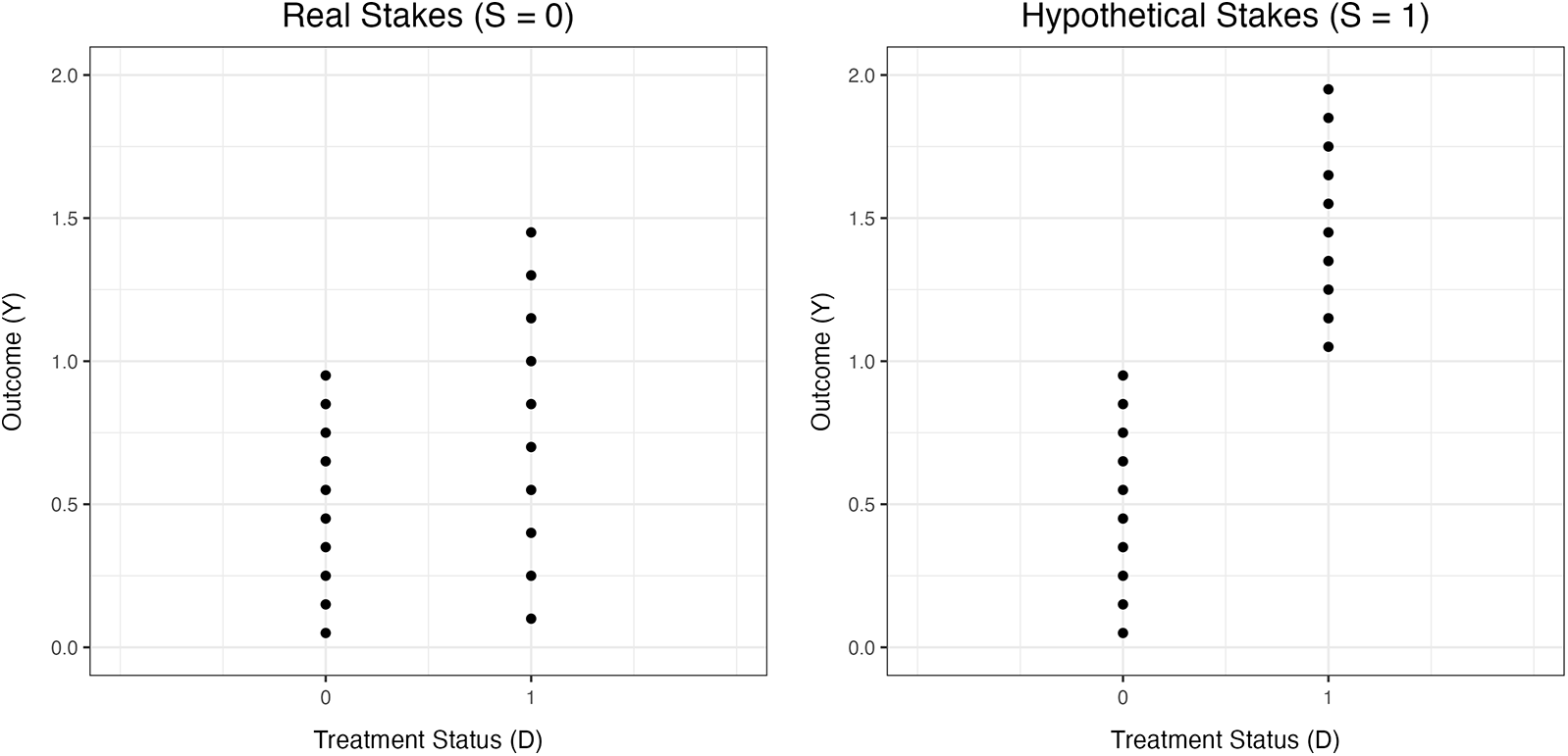


 Open access