


1. Introduction
Univariate parametric statistical models, fitted to historical losses or loss ratios, can be used as a simple way to assess the probabilities of future losses. Commonly used models in actuarial applications include the exponential, log-normal, Weibull, and gamma distributions. The exponential is simple and only has one parameter. Such simplicity may be appropriate, to avoid overfitting, when there is little training data. The log-normal, Weibull, and gamma have two parameters and are more flexible. We will assume that the model is correctly specified, and will not consider issues related to model misspecification, although such issues may be important (Hong & Martin, Reference Hong and Martin2020). A common way to fit the model and make predictions is to determine “best” point estimates of the parameters of the model and substitute those point estimates into the distribution function. Methods for determining point estimates of parameters include maximum likelihood, method of moments, method of L moments, and quantile matching. These point estimate approaches are simple and objective, and are covered in detail in actuarial texts (e.g., Klugman et al., Reference Klugman, Panjer and Willmot2008). However, point estimate predictions of probabilities neglect the uncertainty around the parameter estimates, and this typically leads to an underestimation of the uncertainty in the prediction and an underestimation of extremes. This topic has been discussed by a number of previous authors in the actuarial literature. For instance, Cairns (Reference Cairns2000) emphasizes the need to consider all sources of uncertainty, including parameter uncertainty. Van Kampen (Reference Van Kampen2003) investigates the representation of parameter uncertainty in the log-normal distribution using a bootstrapping methodology and reports that not including parameter uncertainty may result in a material underestimation of the expected loss of stop-loss contracts. Wacek (Reference Wacek2005) discusses formulae that can be used to include parameter uncertainty in the normal and log-normal distributions. England & Verrall (Reference England and Verrall2006) discuss how parameter uncertainty can be modeled using either bootstrapping or Bayesian prediction. Gerrard & Tsanakas (Reference Gerrard and Tsanakas2011) use simulations to quantify the bias from using maximum likelihood to estimate future probabilities, and discuss the objective Bayesian approach of Severini et al. (Reference Severini, Mukerjee and Ghosh2002), which we will also consider below. Bignozzi & Tsanakas (Reference Bignozzi and Tsanakas2016) consider the impact of parameter uncertainty on estimated quantiles and other risk measures. Meanwhile, Fröhlich & Weng (Reference Fröhlich and Weng2015), Fröhlich and Weng (Reference Fröhlich and Weng2018), and Blanco and Weng (Reference Blanco and Weng2019) take a different approach to including parameter uncertainty, based on fiducial probabilities, while Hong & Martin (Reference Hong and Martin2017, Reference Hong and Martin2020) explore nonparametric Bayesian methods which account for prior information, parameter uncertainty, and model misspecification. More recently, Venter & Sahasrabuddhe (Reference Venter and Sahasrabuddhe2021) give a derivation for a Bayesian method for including parameter uncertainty in the Pareto distribution.
We are interested in the question of how to include parameter objectively, i.e., in the absence of prior information. The question of how to include parameter uncertainty in univariate parametric statistical models in an objective way has been discussed in the statistics literature, in particular by Fraser (Reference Fraser1961), Hora & Buehler (Reference Hora and Buehler1966), and Severini et al. (Reference Severini, Mukerjee and Ghosh2002). Severini et al., consider a prediction method in which predictions are generated using the Bayesian prediction equation with an objective prior known as the right Haar prior (RHP). We will refer to this method as RHP prediction. Severini et al., show that RHP predictions give an exact representation of parameter uncertainty, in the sense that the predictions are exactly reliable (we explain the terms in italics in Section 2 below). RHP predictions can be generated for all models with sharply transitive transformation groups, which we call RHP models. As discussed in Gerrard & Tsanakas (Reference Gerrard and Tsanakas2011), the set of RHP models includes all location, scale, and location-scale models, as well as all models that can be derived from location, scale, and location-scale models by positive transformations. In addition, it includes all those models with predictors on the parameters. The set of RHP models therefore includes the exponential, normal, lognormal, logistic, Cauchy, Gumbel, Weibull, one-parameter versions of the gamma and Pareto, a two-parameter version of the Fréchet, the
 $t$
distribution with known degrees of freedom, simple linear regression, and various other less commonly used models. The set of RHP models does not, however, include commonly used models such as the gamma, the generalized Pareto (GPD), the inverse gamma, or the inverse Gaussian.
$t$
distribution with known degrees of freedom, simple linear regression, and various other less commonly used models. The set of RHP models does not, however, include commonly used models such as the gamma, the generalized Pareto (GPD), the inverse gamma, or the inverse Gaussian.
This article has six goals. The first goal is to explain RHP prediction from a group theory perspective, which is an alternative to the location-scale perspective given in Gerrard & Tsanakas (Reference Gerrard and Tsanakas2011). Using this perspective, we demonstrate that the set of RHP models includes models with predictors. The second goal is to provide more detailed quantification of the reliability bias of maximum likelihood predictions, which has previously been quantified in some specific cases by Gerrard & Tsanakas (Reference Gerrard and Tsanakas2011) and Fröhlich & Wang (Reference Fröhlich and Weng2015). The third goal is to test methods for making predictions for a number of models that are used in actuarial science, but that are not covered by RHP theory. We consider the gamma, GPD, inverse gamma, and inverse Gaussian. For these models, we test whether we can reduce the bias relative to the bias of maximum likelihood predictions by using Bayesian predictions with carefully chosen priors. The fourth goal is to explore practical numerical schemes for making Bayesian predictions. The fifth goal is to present an example, using hurricane loss data, that illustrates the impact of modeling with parameter uncertainty, and the sixth goal is to introduce a software library which contains simple commands that can be used to generate all the predictions that we discuss.
In Section 2, we explain RHP prediction. In Section 3, we derive various RHPs and give the priors we will test for the non-RHP models we consider. In Section 4, we discuss methods for making Bayesian predictions, including the use of closed-form expressions based on an asymptotic expansion. In Section 5, we use simulations to test different prediction methods in terms of the level of reliability that they achieve. In Section 6, we give an example, using hurricane loss data, that illustrates the impact of including parameter uncertainty in predictions. In Section 7, we discuss predictive means, and in Section 8, we conclude. Finally, in the appendix, we give some additional results and a brief description of the fitdistcp software package, which implements the methods we describe.
2. RHP prediction
We discuss reliability, transformation groups, Haar’s theorem, and predictive invariance before stating the Severini et al., theorem that is the basis for RHP prediction.
2.1 Reliability
To explain reliability, we imagine evaluating a prediction method by applying the method repeatedly to different simulated sets of training data. For each set of training data, we make predictions of exceedance quantiles at specified probabilities that we call the nominal probabilities. We then use the known distribution function for the model to calculate the proportion of future values that exceed each predicted exceedance quantile and average that proportion over all sets of training data. The limit of this proportion, as the number of tests tends to infinity, is known as the predictive coverage probability (PCP), since it measures the extent to which the prediction covers future outcomes. For a finite number of tests, the average proportion gives a Monte Carlo estimate of the PCP. The effectiveness of the prediction method is then evaluated by comparing the PCPs with the corresponding nominal probabilities. When the PCP and nominal probabilities are equal, the prediction method is reliable. For instance, when using a reliable prediction method, the proportion of future values that exceed the predictions for the 1% exceedance quantile converges to 1%. For a prediction that is not reliable, and consistently underpredicts the tail, the proportion of future values that exceed the predictions for the 1% exceedance quantile will converge to greater than 1%.
In Section 5, we perform simulations, along the lines of the description above, to test various predictions.
2.2 Sharply transitive transformation models
RHP prediction only applies to sharply transitive transformation models. We will explain what defines a sharply transitive transformation model using the normal distribution as an example.
If we transform a normally distributed random variable
 $X$
using the transformation
$X$
using the transformation
 $X'=a+bX$
, where
$X'=a+bX$
, where
 $a$
is a real number and
$a$
is a real number and
 $b$
is a positive real number, then the new random variable
$b$
is a positive real number, then the new random variable
 $X'$
will also be normally distributed. The mean and standard deviation transform from
$X'$
will also be normally distributed. The mean and standard deviation transform from
 $(\mu ,\sigma )$
to
$(\mu ,\sigma )$
to
 $(\mu ',\sigma ')$
as
$(\mu ',\sigma ')$
as
 $\mu '=a+b\mu$
and
$\mu '=a+b\mu$
and
 $\sigma '=b\sigma$
. The set of all transformations, indexed by
$\sigma '=b\sigma$
. The set of all transformations, indexed by
 $(a,b)$
, forms a group, and the action of this group on the set of normal distributions, indexed by
$(a,b)$
, forms a group, and the action of this group on the set of normal distributions, indexed by
 $(\mu ,\sigma )$
, is a group action. Because there are transformations in the group that can transform any normal into any other, the group action is described as transitive. Furthermore, because there is only one transformation that can transform a given normal into another given normal, the group action is described as sharply transitive, and we describe the normal as a sharply transitive transformation model. For such sharply transitive transformation models, a (non-unique) bijection can be constructed between the elements of the transformation group and the elements of the set of distributions. Via this bijection, the set of distributions can be considered to inherit the group structure, and hence is also a group. For instance, for the normal, a bijection can be constructed by identifying the transformation given by parameters
$(\mu ,\sigma )$
, is a group action. Because there are transformations in the group that can transform any normal into any other, the group action is described as transitive. Furthermore, because there is only one transformation that can transform a given normal into another given normal, the group action is described as sharply transitive, and we describe the normal as a sharply transitive transformation model. For such sharply transitive transformation models, a (non-unique) bijection can be constructed between the elements of the transformation group and the elements of the set of distributions. Via this bijection, the set of distributions can be considered to inherit the group structure, and hence is also a group. For instance, for the normal, a bijection can be constructed by identifying the transformation given by parameters
 $(a,b)$
with the distribution given by the parameters
$(a,b)$
with the distribution given by the parameters
 $(\mu =a,\sigma =b)$
. The group operation is given by the transformation rule, such that two group elements
$(\mu =a,\sigma =b)$
. The group operation is given by the transformation rule, such that two group elements
 $(\mu ,\sigma )$
and
$(\mu ,\sigma )$
and
 $(m,s)$
combine as
$(m,s)$
combine as
 $(\mu ,\sigma )*(m,s)=(\mu +\sigma m,\sigma s)$
. This operation is not commutative. It is the set of distributions forming a group in this way that is the key feature required for RHP prediction.
$(\mu ,\sigma )*(m,s)=(\mu +\sigma m,\sigma s)$
. This operation is not commutative. It is the set of distributions forming a group in this way that is the key feature required for RHP prediction.
Some statistical models have associated sharply transitive transformation groups, as the normal does; some have associated transformation groups that are not transitive, and some do not have transformation groups. For instance, location models, scale models, and location-scale models all have sharply transitive transformation groups. Also, models related to location, scale, and location-scale models by positive transformations have sharply transitive transformation groups. On the other hand, the gamma, GPD, inverse gamma, and inverse Gaussian have transformation groups, but do not have transitive transformation groups, while the gamma with known scale parameter does not have a transformation group.
2.3 Haar’s theorem
These transformation groups are examples of locally compact Hausdorff topological groups, and a theorem from the intersection of group theory and measure theory known as Haar’s theorem (Haar, Reference Haar1933) states that for each such group there exist two invariant measures, the left and right Haar measures. The left (right) Haar measure has the property that the measure of a subset of the group remains the same after left (right) multiplication by any element of the group. In Bayesian statistics, these measures are referred to as the left Haar prior (LHP) and RHP (Fraser, Reference Fraser1961; Hora & Buehler, Reference Hora and Buehler1966; Berger, Reference Berger2006). For the normal distribution, the invariance property means that the integral of the left (right) Haar prior, over a subset of the two dimensional space of all normal distributions, indexed by
 $(\mu ,\sigma )$
, remains the same even if the subset is left (right) multiplied by any group element. In simple cases, when the transformation is commutative, the LHP and RHP are the same. For instance, for the exponential distribution, the LHP and RHP are the same, while for the normal distribution they are different. The RHP has two properties that make it of interest for prediction: prediction invariance and reliability of predictions, which we discuss below.
$(\mu ,\sigma )$
, remains the same even if the subset is left (right) multiplied by any group element. In simple cases, when the transformation is commutative, the LHP and RHP are the same. For instance, for the exponential distribution, the LHP and RHP are the same, while for the normal distribution they are different. The RHP has two properties that make it of interest for prediction: prediction invariance and reliability of predictions, which we discuss below.
2.4 Prediction invariance
A Bayesian prediction made using either the LHP or RHP as the prior is invariant to parameter transformations from the transformation group for that model. For instance, for the normal distribution, predictions made using the RHP or LHP for the normal will be the same before and after reparametrisation using
 $\mu '=a+b\mu , \sigma '=b\sigma$
. As an example, if we are using the normal distribution to represent temperatures, then a prediction of the probability of freezing temperatures would be the same whether the prediction is made using Celsius or Fahrenheit. This is because the conversion between Celsius and Fahrenheit is an example of a transformation from the transformation group for the normal distribution.
$\mu '=a+b\mu , \sigma '=b\sigma$
. As an example, if we are using the normal distribution to represent temperatures, then a prediction of the probability of freezing temperatures would be the same whether the prediction is made using Celsius or Fahrenheit. This is because the conversion between Celsius and Fahrenheit is an example of a transformation from the transformation group for the normal distribution.
2.5 Reliability of predictions
The Severini et al., theorem that forms the basis for RHP prediction states that Bayesian predictions for models with a sharply transitive transformation group, made using the RHP, will be reliable. In other words, in repeated testing, the PCP will match the nominal probability, and the set of events that are predicted to occur with a probability of
 $p\%$
will occur
$p\%$
will occur
 $p\%$
of the time, for all
$p\%$
of the time, for all
 $p$
. This is true for all parameter values individually, and a method that gives reliable predictions for all parameter values individually will give reliable predictions even when the parameter is unknown.
$p$
. This is true for all parameter values individually, and a method that gives reliable predictions for all parameter values individually will give reliable predictions even when the parameter is unknown.
3. Priors
We now derive RHPs for a number of models, and also give the priors we will use in our attempts to generate reliable predictions for a number of distributions that do not have sharply transitive transformation groups.
3.1 Right Haar priors
To apply the Severini et al., theory to prediction, for a model which has a sharply transitive transformation group, we need to know the RHP for that model. The RHP can be derived from the transformation group using the formula:
 \begin{eqnarray} \pi (\theta ) \propto \left | \frac {\partial {(t\theta )}}{\partial {t}}{(t=e)} \right |_{+}^{-1} \end{eqnarray}
where
 $\theta$
is the parameter vector,
$\theta$
is the parameter vector,
 $\pi (\theta )$
is the RHP,
$\pi (\theta )$
is the RHP,
 $t$
is a vector representing the parameter transformation,
$t$
is a vector representing the parameter transformation,
 $t\theta$
is the transformation applied to the parameter vector, and
$t\theta$
is the transformation applied to the parameter vector, and
 $e$
is the identity element of the transformation group. The plus sign indicates that the absolute value of the determinant is taken. This formula can be derived from the definition of the RHP.
$e$
is the identity element of the transformation group. The plus sign indicates that the absolute value of the determinant is taken. This formula can be derived from the definition of the RHP.
The RHPs for some commonly used RHP models can be derived as follows.
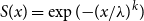
3.1.1 Exponential distribution
For the exponential, with exceedance distribution function given by
 $S(x)=\exp ({-}\lambda x)$
, the parameter transformation is
$S(x)=\exp ({-}\lambda x)$
, the parameter transformation is
 $\lambda '=b\lambda$
and the RHP is
$\lambda '=b\lambda$
and the RHP is
 \begin{eqnarray} \pi (\lambda ) \propto \left | \frac {\partial {(b\lambda )}}{\partial {b}}{(b=1)} \right |_{+}^{-1} =\frac {1}{\lambda } \end{eqnarray}
For any scale model with scale parameter
 $\sigma$
, the transformation is
$\sigma$
, the transformation is
 $\sigma '=b\sigma$
and the RHP is
$\sigma '=b\sigma$
and the RHP is
 \begin{eqnarray} \pi (\sigma ) \propto \left | \frac {\partial {(b\sigma )}}{\partial {b}}{(b=1)} \right |_{+}^{-1} =\frac {1}{\sigma } \end{eqnarray}
3.1.2 Pareto distribution
For the Pareto distribution with fixed scale parameter
 $x_m$
and exceedance distribution function given by
$x_m$
and exceedance distribution function given by
 $S(x)=(x_m/x)^\alpha$
, which we will call the Pareto distribution, the transformation is
$S(x)=(x_m/x)^\alpha$
, which we will call the Pareto distribution, the transformation is
 $\alpha '=c\alpha$
and the RHP is
$\alpha '=c\alpha$
and the RHP is
 \begin{eqnarray} \pi (\alpha ) \propto \left | \frac {\partial {(c\alpha )}}{\partial {c}}{(c=1)} \right |_{+}^{-1} =\frac {1}{\alpha } \end{eqnarray}
3.1.3 Normal distribution
For the normal distribution parametrized using mean
 $\mu$
and standard deviation
$\mu$
and standard deviation
 $\sigma$
, the transformation is
$\sigma$
, the transformation is
 $\mu '=a+b\mu , \sigma '=b\sigma$
, as given above, and the RHP is
$\mu '=a+b\mu , \sigma '=b\sigma$
, as given above, and the RHP is
 \begin{eqnarray} \pi (\mu ,\sigma ) \propto \left | \frac {\partial {(a+b\mu ,b\sigma )}}{\partial {(a,b)}}{((a,b)=(0,1))} \right |_{+}^{-1} = \left | \begin{pmatrix} 1 &\quad \mu \\[2pt] 0 &\quad \sigma \end{pmatrix} \right |_{+}^{-1} =\frac {1}{\sigma } \end{eqnarray}
For any other location-scale model, parametrized using location parameter
 $\mu$
and scale parameter
$\mu$
and scale parameter
 $\sigma$
, the transformation and the RHP are the same as for the normal distribution. Examples are the Gumbel, logistic, and Cauchy distributions, and the generalized extreme value distribution (GEVD) and GPD with known shape parameter.
$\sigma$
, the transformation and the RHP are the same as for the normal distribution. Examples are the Gumbel, logistic, and Cauchy distributions, and the generalized extreme value distribution (GEVD) and GPD with known shape parameter.
3.1.4 Log-normal distribution
For the log-normal distribution, the transformation and RHP are the same as for the normal distribution. Any other log location-scale model also has the same transformation and RHP. Examples are the log-Gumbel, log-logistic, log-Cauchy distributions, and the log-GEVD with known shape parameter.
3.1.5 Fréchet distribution
For the Fréchet distribution with zero location parameter, which we will refer to simply as the Fréchet distribution, and which has cumulative distribution function given by
 $F(x)=\exp ({-}{(x/s)}^{-\alpha })$
, the transformation is
$F(x)=\exp ({-}{(x/s)}^{-\alpha })$
, the transformation is
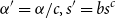 $\alpha '=\alpha /c, s'=bs^c$
and the RHP is
$\alpha '=\alpha /c, s'=bs^c$
and the RHP is
 \begin{eqnarray} \pi (s,\alpha ) \propto \left | \frac {\partial {(\alpha /c,bs^c)}}{\partial {(b,c)}}{((b,c)=(1,1))} \right |_{+}^{-1} = \left | \begin{pmatrix} 0 &\quad -\alpha \\ s &\quad s\log (s) \end{pmatrix} \right |_{+}^{-1} =\frac {1}{s\alpha } \end{eqnarray}
This prior can also be obtained by transformation of the Frćhet distribution to a location-scale model along with appropriate transformations of the location and scale parameters (see Gerrard & Tsanakas, Reference Gerrard and Tsanakas2011 for a discussion of this approach).
3.1.6 Weibull distribution
For the Weibull distribution, with exceedance distribution function given by
 $S(x)=\exp ({-}{(x/\lambda )}^k)$
, the transformation is
$S(x)=\exp ({-}{(x/\lambda )}^k)$
, the transformation is
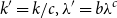 $k'=k/c, \lambda '=b\lambda ^c$
. This is analogous to the transformation for the Fréchet, and so the RHP is
$k'=k/c, \lambda '=b\lambda ^c$
. This is analogous to the transformation for the Fréchet, and so the RHP is
 $\pi (k,\lambda ) = 1/(k \lambda )$
.
$\pi (k,\lambda ) = 1/(k \lambda )$
.
3.1.7 Location predictors
If
 $m$
predictors
$m$
predictors
 $u_i$
are added to any of the location parameters in the above models, with the form:
$u_i$
are added to any of the location parameters in the above models, with the form:
 \begin{equation*} \mu =\beta _0+\sum _{i=1}^m \beta _i u_i \end{equation*}
where
 $\beta _i$
are scalar parameters, then the model is still a sharply transitive transformation model, and Equation (1) shows that the RHP remains the same. For instance, for a location-scale model with single predictor
$\beta _i$
are scalar parameters, then the model is still a sharply transitive transformation model, and Equation (1) shows that the RHP remains the same. For instance, for a location-scale model with single predictor
 $u$
, location
$u$
, location
 $\alpha +\beta u$
and scale
$\alpha +\beta u$
and scale
 $\sigma$
, the transformation
$\sigma$
, the transformation
 $t=(a,b,c)$
is
$t=(a,b,c)$
is
 \begin{align} x' &=a+bu+cx \end{align}
 \begin{align} \alpha ' &=a+c\alpha \end{align}
 \begin{align} \beta ' &=b+c\beta \end{align}
 \begin{align} \sigma ' &=c\sigma \\[6pt] \nonumber \end{align}
and the RHP is
 \begin{align} \pi (\alpha ,\beta ,\sigma ) &\propto \left | \frac {\partial {(a+c\alpha ,b+c\beta ,c\sigma )}} {\partial {(a,b,c)}}{((a,b,c)=(0,0,1))} \right |_{+}^{-1} \end{align}
 \begin{align} &= \left | \begin{pmatrix} 1 & \quad 0 & \quad \alpha \\ 0 & \quad 1 & \quad \beta \\ 0 & \quad 0 & \quad \sigma \end{pmatrix} \right |_{+}^{-1}\end{align}
 \begin{align} &= \frac {1}{\sigma } \\[6pt] \nonumber\end{align}
3.1.8 Scale predictors
If
 $m$
predictors
$m$
predictors
 $v_i$
are added to any of the scale parameters and the scale parameter
$v_i$
are added to any of the scale parameters and the scale parameter
 $\sigma$
is replaced so that
$\sigma$
is replaced so that
 \begin{equation*} \sigma \rightarrow \sigma \exp \left (\sum _{i=1}^m \delta _i v_i\right ) \end{equation*}
where
 $\delta _i$
are scalar parameters, then the model is still a sharply transitive transformation model, and the RHP remains the same.
$\delta _i$
are scalar parameters, then the model is still a sharply transitive transformation model, and the RHP remains the same.
For instance, for a location-scale model with single predictor
 $v$
, location
$v$
, location
 $\mu$
and scale
$\mu$
and scale
 $\sigma \exp (\delta v)$
, the transformation
$\sigma \exp (\delta v)$
, the transformation
 $t=(a,c,d)$
is
$t=(a,c,d)$
is
 \begin{align} x'&=a+cx\exp (d v) \end{align}
 \begin{align} \mu '&=a+c\mu \exp (d v) \end{align}
 \begin{align} \sigma '&=c\sigma \end{align}
 \begin{align} \delta '&=d+\delta \\[6pt] \nonumber\end{align}
The RHP for this model,
 $\pi (\theta )=\pi (\mu ,\sigma ,\delta )$
, is derived as follows:
$\pi (\theta )=\pi (\mu ,\sigma ,\delta )$
, is derived as follows:
 \begin{align} \pi (\theta ) &\propto \left | \frac {\partial {(a+c\mu \exp (d v),c\sigma ,d+\delta )}} {\partial {(a,c,d)}}{((a,c,d)=(0,1,0))} \right |_{+}^{-1} \end{align}
 \begin{align} &= \left | \begin{pmatrix} 1 &\quad \mu & \quad \mu v\\ 0 & \quad \sigma & \quad 0\\ 0 & \quad 0 & \quad 1 \end{pmatrix} \right |_{+}^{-1} \end{align}
 \begin{align} &= \frac {1}{\sigma } \\[6pt] \nonumber\end{align}
3.1.9 Location and scale predictors
Different predictors can also be added to two parameters at the same time, using the above expressions, and the model will still be a sharply transitive transformation model, and the prior will not change.
For instance, for a location-scale model with predictors
 $u, v$
, location
$u, v$
, location
 $\alpha +\beta u$
and scale
$\alpha +\beta u$
and scale
 $\sigma \exp (\delta v)$
, the transformation
$\sigma \exp (\delta v)$
, the transformation
 $t=(a,b,c,d)$
is
$t=(a,b,c,d)$
is
 \begin{align} x'&=a+bu+cx\exp (d v) \end{align}
 \begin{align} \alpha '&=a+c\alpha \exp (d v) \end{align}
 \begin{align} \beta '&=b+c\beta \exp (d v) \end{align}
 \begin{align} \sigma '&=c\sigma \end{align}
 \begin{align} \delta '&=d+\delta \\[6pt] \nonumber\end{align}
The RHP for this model,
 $\pi (\theta )=\pi (\alpha ,\beta ,\sigma ,\delta )$
, is derived as follows:
$\pi (\theta )=\pi (\alpha ,\beta ,\sigma ,\delta )$
, is derived as follows:
 \begin{align} \pi (\theta ) &\propto \left | \frac {\partial {(a+c\alpha \exp (d v),b+c\beta \exp (d v),c\sigma ,d+\delta )}} {\partial {(a,b,c,d)}}{(t=(0,0,1,0))} \right |_{+}^{-1} \end{align}
 \begin{align} &= \left | \begin{pmatrix} 1 & \quad 0 & \quad \alpha & \quad \alpha v\\ 0 & \quad 1 & \quad \beta & \quad \beta v\\ 0 & \quad 0 & \quad \sigma & \quad 0\\ 0 & \quad 0 & \quad 0 & \quad 1 \end{pmatrix} \right |_{+}^{-1} \end{align}
 \begin{align} &= \frac {1}{\sigma } \\[6pt] \nonumber\end{align}
Predictors can be added, in a similar way, to the scale and shape parameters of the Fréchet and Weibull distributions.
3.2 Non RHP models
RHP prediction only applies to models with sharply transitive transformation groups. For models such as the gamma, GPD, inverse gamma, or inverse Gaussian, which lack transitive transformation groups, the theory does not apply. For these models, a pragmatic approach to generating predictions that include parameter uncertainty is to test various priors using simulations and attempt to find priors that give reasonable reliability. We test the following priors:
-
• For the gamma, with density given by
 $x^{k-1}\exp ({-}x/\sigma )/(\Gamma (k)\sigma ^k)$
, we test
$\pi _1(k,\sigma ) = 1/(k \sigma )$
and
$\pi _2(k,\sigma ) = 1/\sigma$
.
$x^{k-1}\exp ({-}x/\sigma )/(\Gamma (k)\sigma ^k)$
, we test
$\pi _1(k,\sigma ) = 1/(k \sigma )$
and
$\pi _2(k,\sigma ) = 1/\sigma$
. -
• for the GPD, with exceedance distribution function given by
$(1+\xi z)^{-1/\xi }$
, where
$\xi =(x-\mu )/\sigma$
, and
$\mu$
is constant, we test
$\pi (\sigma ,\xi ) = 1/\sigma$
. -
• For the inverse gamma, with density given by
$x^{-\alpha -1}\exp ({-}\sigma /x)\sigma ^\alpha /\Gamma (\alpha )$
, we test
$\pi _1(\alpha ,\sigma ) = 1/(\alpha \sigma )$
and
$\pi _2(\alpha ,\sigma ) = 1/\sigma$
. -
• For the inverse Gaussian, with density given by
$\sqrt {\lambda /(2\pi x^3)} \exp \left [-\lambda (x-\mu )^2/(2\mu ^2x)\right ]$
, we test
$\pi _1(\mu ,\lambda ) = 1/(\mu \lambda )$
and
$\pi _2(\mu ,\lambda ) = 1/\lambda$
.


4. Making Bayesian predictions
To make a Bayesian prediction, we have to evaluate the posterior predictive distribution of a future loss
 $Y$
given training data
$Y$
given training data
 $x$
. The associated predictive density is given by:
$x$
. The associated predictive density is given by:
 \begin{align} p(y|x)=\frac {\int f(y;\;\theta ) L(\theta ;\;x) \pi (\theta ) d\theta } {\int L(\theta ;\;x) \pi (\theta ) d\theta } \end{align}
where
 $f(y;\;\theta )$
is the probability density of
$f(y;\;\theta )$
is the probability density of
 $Y$
given parameters
$Y$
given parameters
 $\theta$
,
$\theta$
,
 $L(\theta ;\;x)$
is the likelihood function and
$L(\theta ;\;x)$
is the likelihood function and
 $\pi (\theta )$
is the prior density of
$\pi (\theta )$
is the prior density of
 $\theta$
.
$\theta$
.
In principle, any method of integration can be used to evaluate Equation 29. In practice, different methods have different strengths and weaknesses, depending on the particular problem. We now briefly review five methods one can use to evaluate this expression.
4.1 Analytic solutions
For some models, the posterior predictive density given by Equation 29 has a closed form. Wacek (Reference Wacek2005), and also statistical sources such as Lee (Reference Lee2012) and Bernardo & Smith (Reference Bernardo and Smith1993), give the exact solution for the normal distribution, which is a form of the Student
 $t$
distribution. Predictions for the log-normal can then be made by taking the log of the data and using the formula for the normal. Venter & Sahasrabuddhe (Reference Venter and Sahasrabuddhe2021), and Bernardo & Smith (Reference Bernardo and Smith1993), give the exact solution for the exponential distribution, which is a form of the Pareto distribution. The exact solution for the Pareto distribution can be derived from the formula for the exponential by substituting
$t$
distribution. Predictions for the log-normal can then be made by taking the log of the data and using the formula for the normal. Venter & Sahasrabuddhe (Reference Venter and Sahasrabuddhe2021), and Bernardo & Smith (Reference Bernardo and Smith1993), give the exact solution for the exponential distribution, which is a form of the Pareto distribution. The exact solution for the Pareto distribution can be derived from the formula for the exponential by substituting
 $x_{exponential}=\log (x_{pareto}/x_m)$
, where
$x_{exponential}=\log (x_{pareto}/x_m)$
, where
 $x_m$
is a lower bound.
$x_m$
is a lower bound.
4.2 Numerical integration
For models for which the Bayesian prediction equation cannot be solved analytically, other methods must be used. For models with a very small number of parameters, deterministic numerical integration methods, such as Gaussian quadrature, may be appropriate. However, Gaussian quadrature requires the specification of limits of integration and integration points. It therefore requires some expertize to use and is difficult to automate. It becomes computationally inefficient for models with multiple parameters.
4.3 Markov chain Monte Carlo
A general-purpose set of numerical simulation algorithms for performing the integration is the various Markov Chain Monte Carlo (MCMC) algorithms (Bailer-Jones, Reference Bailer-Jones2017). These algorithms simulate samples from the distribution for the parameter vector
 $\theta$
. Samples from the distribution for
$\theta$
. Samples from the distribution for
 $Y$
can be generated by sampling from the distribution function for each sampled value of
$Y$
can be generated by sampling from the distribution function for each sampled value of
 $\theta$
. Predictive densities and probabilities can be generated by averaging over density and distribution functions based on the samples for
$\theta$
. Predictive densities and probabilities can be generated by averaging over density and distribution functions based on the samples for
 $\theta$
. Predictive quantiles can be generated by sorting the samples for
$\theta$
. Predictive quantiles can be generated by sorting the samples for
 $Y$
to create an empirical distribution function and then inverting that function numerically. Two of the advantages of MCMC are that it is widely available in software packages, and can be used for almost any model. However, MCMC requires certain parameters to be set, and it also requires a suitable burn-in period before the distribution of the samples can be considered to have converged to the distribution for
$Y$
to create an empirical distribution function and then inverting that function numerically. Two of the advantages of MCMC are that it is widely available in software packages, and can be used for almost any model. However, MCMC requires certain parameters to be set, and it also requires a suitable burn-in period before the distribution of the samples can be considered to have converged to the distribution for
 $\theta$
. As a result, MCMC also requires some expertize to use and is difficult to automate. It may also not be the fastest method for sampling the distribution for
$\theta$
. As a result, MCMC also requires some expertize to use and is difficult to automate. It may also not be the fastest method for sampling the distribution for
 $\theta$
for models with a small number of parameters.
$\theta$
for models with a small number of parameters.
4.4 Rejection sampling
For models with small numbers of parameters, rejection sampling, and in particular the ratio of uniforms with transformation (RUST) rejection sampling algorithm (Wakefield et al., Reference Wakefield, Gelfand and Smith1991), can also be used to generate samples from the distribution for
 $\theta$
. Rejection sampling may be faster than MCMC for models with a small number of parameters, and does not require a burn-in period. It is simple to use and well-suited for automation.
$\theta$
. Rejection sampling may be faster than MCMC for models with a small number of parameters, and does not require a burn-in period. It is simple to use and well-suited for automation.
4.5 Asymptotic approximation
A fifth method for generating the Bayesian prediction is to use asymptotic expressions for the density, distribution function, and quantiles of
 $Y$
. We will use the asymptotic expressions given in Datta et al. (Reference Datta, Mukerjee, Ghosh and Sweeting2000), and we refer to using these expressions as the DMGS method, based on the authors’ initials. These expressions have the advantage that they are fast to evaluate. The advantage is largest for predictive quantiles, for which the other numerical methods are particularly slow because of the need to invert an empirical distribution, which DMGS avoids. DMGS has the disadvantage that the approximation may not be sufficiently accurate for small sample sizes (i.e., fewer than 10 or 20 data points), depending on the application.
$Y$
. We will use the asymptotic expressions given in Datta et al. (Reference Datta, Mukerjee, Ghosh and Sweeting2000), and we refer to using these expressions as the DMGS method, based on the authors’ initials. These expressions have the advantage that they are fast to evaluate. The advantage is largest for predictive quantiles, for which the other numerical methods are particularly slow because of the need to invert an empirical distribution, which DMGS avoids. DMGS has the disadvantage that the approximation may not be sufficiently accurate for small sample sizes (i.e., fewer than 10 or 20 data points), depending on the application.
We will use the DMGS method below in our simulation experiments in which we evaluate predictive quantiles from the prediction integral many times for different random samples in order to evaluate the degree of reliability. It is the speed of the DMGS equation for calculating predictive quantiles that makes our reliability analysis computationally feasible for those models for which there is no analytic expression.
The DMGS method also has other useful features: it can be used to generate an approximation to the Fourier transform of the predictive distribution and approximate closed-form expressions for the mean and variance of the predictive distribution.
5. Simulation testing
We now test the reliability of predictions for various models using simulations. For each model, we test maximum likelihood and Bayesian predictions. For the Bayesian predictions, we use calibrating priors consisting of the RHP for RHP models and the priors given in Section 3.2 for non-RHP models.
5.1 RHP models
We test maximum likelihood and RHP predictions for the exponential, Pareto, log-normal, Weibull, and Fréchet models. For the exponential, Pareto and log-normal we generate the RHP predictions using exact analytical expressions, and we would expect to see exact reliability. For the Weibull and Fréchet distributions, we generate the RHP predictions using the DMGS method, and might therefore expect to see a divergence from exact reliability due to the approximation involved in that method.
We consider training data sample sizes of 20 and 50 to assess the effect of sample size on the results. The sample size of 50 is chosen to be close to the sample size used in our example in Section 5 below (which has a sample size of 51). We present the results in both figures and tables. For the figures, we simulate 10,000 training samples in each test, and repeat each test 3 times to ensure that we have achieved reasonable convergence. For the tables, we simulate 100,000 training samples once. Fraser (Reference Fraser1961) and Gerrard & Tsanakas (Reference Gerrard and Tsanakas2011) have given mathematical derivations that show that the simulation results for the RHP models do not depend on the values of the parameters used for these tests. As a result, we only need to test one set of parameter values. We set the parameters to 0 for location and log-location parameters and 1 for scale and log-scale parameters. We set the shape parameter of the Pareto to 1, the shape parameter of the Weibull to 3, and the shape parameter of the Fréchet to 3. Our simulation approach is slightly different from that used by Gerrard & Tsanakas (Reference Gerrard and Tsanakas2011), in that we do not simulate values of
 $y$
, the variable being predicted, but use the known distribution function to evaluate probability of exceeding the predicted exceedance quantiles. This requires fewer simulations to achieve the same level of convergence.
$y$
, the variable being predicted, but use the known distribution function to evaluate probability of exceeding the predicted exceedance quantiles. This requires fewer simulations to achieve the same level of convergence.

Figure 1 Monte Carlo estimates of predictive coverage probabilities (PCPs) versus nominal probabilities for five commonly used distributions. The axes are linearly spaced in inverse exceedance probability. The Pareto is a one-parameter distribution with known scale parameter. The Fréchet is a two-parameter distribution with known location parameter. In each case, predictions are made using maximum likelihood (3 gray lines) and right Haar prior predictions (3 black lines). For exponential, Pareto, and log-normal distributions, the RHP predictions are made using closed-form evaluation of the Bayesian prediction equation. For Fréchet and Weibull distributions, the RHP predictions are made using the DMGS asymptotic approximation for predictive quantiles. The training data consists of 20 values in each case, repeated 10,000 times to estimate the PCPs. Each test is then repeated 3 times to assess convergence. The sets of 3 lines look like a single line in most cases, indicating adequate convergence.
Figure 1, and Table A.1 in Appendix A, show results from the simulation experiment with sample size of 20. We see that for the predictions based on maximum likelihood, the PCP is higher than the nominal probability, with large differences in the upper tail. In other words, maximum likelihood predicted quantiles are exceeded more often than one would expect based on the nominal probability. We conclude that maximum likelihood underestimates the tail of the prediction on average, agreeing with the results in Gerrard & Tsanakas (Reference Gerrard and Tsanakas2011) and Fröhlich and Wang (Reference Fröhlich and Weng2015).
The RHP predictions perform much better than the maximum likelihood predictions. For the exponential, Pareto, and log-normal distributions, the RHP predictions give almost exact agreement between the PCP and nominal probabilities, as expected. Any lack of agreement is due to insufficient sampling. For the Fréchet and Weibull, we see that the PCPs are slightly higher than the nominal probabilities. This is because we have used the DMGS method. The reliability bias from using the DMGS method is, however, seen to be much smaller than the reliability bias from using maximum likelihood. This reliability bias could be eliminated by using RUST or MCMC, although that would be much slower to evaluate.
Figure 2, and Table A.2 in Appendix A, show results from the simulation experiment with sample size of 50. The larger sample size improves the maximum likelihood predictions, although they still show significant underestimation in the tail. The larger sample size also improves the Fréchet and Weibull RHP predictions because the asymptotic approximation in the DMGS method is more accurate for larger sample sizes.

Figure 2 As Figure 1, but now for training data sample sizes of 50.
5.2 Gamma distribution
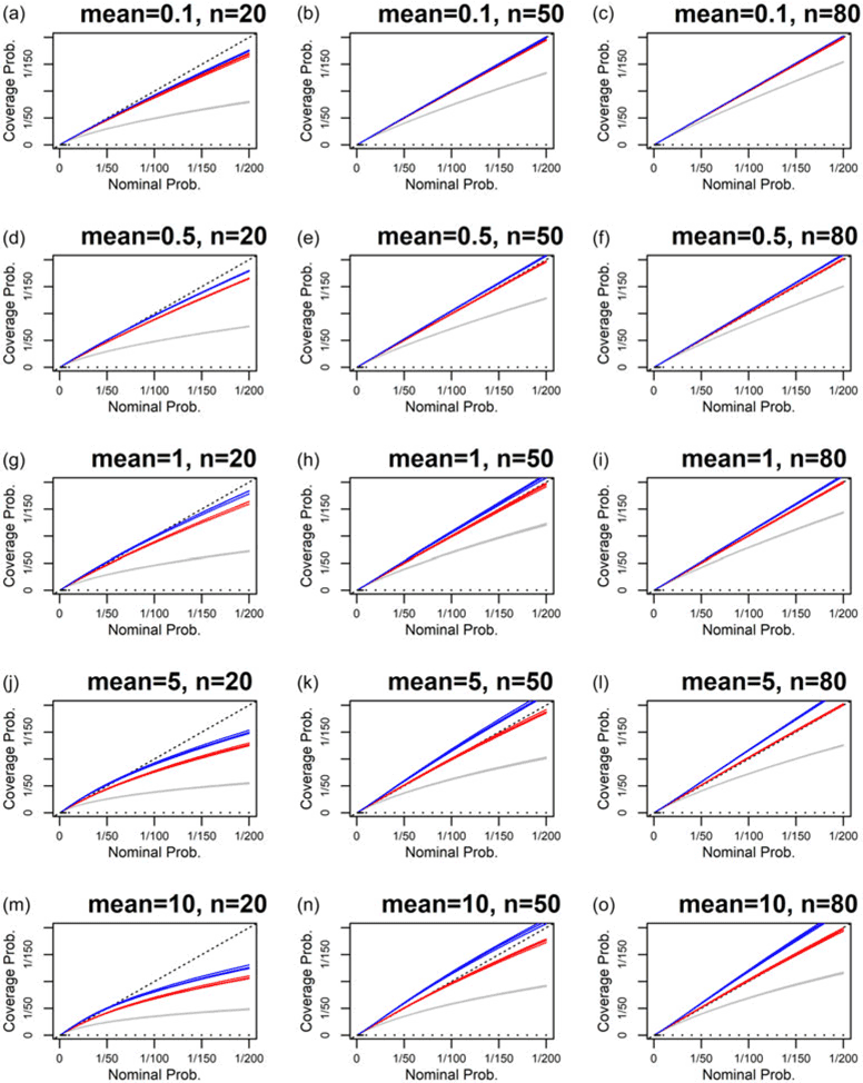
We now test predictions for the gamma distribution, using the two priors given in Section 3.2 above. Figure 3 shows the level of reliability for gamma predictions from maximum likelihood and these priors, as a function of sample size and the gamma shape parameter. For the tail probabilities shown, we see that maximum likelihood underestimates tail probabilities, and that the two Bayesian predictions give better reliability than maximum likelihood in all cases. Of the two priors,
 $\pi _1$
gives better results. For this prior, for a sample size of 20, and for small values of the shape parameter, the reliability is fairly poor, while for a sample size of 80, and for large values of the shape parameter, the reliability is good.
$\pi _1$
gives better results. For this prior, for a sample size of 20, and for small values of the shape parameter, the reliability is fairly poor, while for a sample size of 80, and for large values of the shape parameter, the reliability is good.
We have succeeded in finding a reasonable calibrating prior for predicting the gamma, for sample sizes of 50 and 80 and larger values of the shape parameter. For smaller sample sizes and smaller values of the shape parameter, the results are less good, but still much better than maximum likelihood. Finding a better way to predict the gamma for small sample sizes is an open research question.

Figure 3 As Figure 1, but now for the gamma distribution, for predictions based on maximum likelihood (3 gray lines) and test priors
 $\pi _1$
(red) and
$\pi _1$
(red) and
 $\pi _2$
(blue). For the test priors, predictions are evaluated using the DMGS approximation for predictive quantiles. Each column represents one sample size, for sample sizes of 20, 50, and 80 from left to right. Each row represents one value of the true gamma shape parameter
$\pi _2$
(blue). For the test priors, predictions are evaluated using the DMGS approximation for predictive quantiles. Each column represents one sample size, for sample sizes of 20, 50, and 80 from left to right. Each row represents one value of the true gamma shape parameter
 $k$
, with values from top to bottom of
$k$
, with values from top to bottom of
 $\xi =0.1, 0.5, 1, 5, 10$
.
$\xi =0.1, 0.5, 1, 5, 10$
.
5.3 Generalized Pareto distribution
We now test predictions for the GPD with known location parameter, using the prior given in Section 3.2 above. Figure 4 shows the level of reliability for GPD predictions achieved using this prior. For the tail probabilities shown, we see that these predictions give better reliability than maximum likelihood in all cases. However, for sample size of 20, the prior gives relatively poor results, in which the PCP differs significantly from the nominal probability for both small and large values of
 $\xi$
. For sample size of 50, the results are better, with smaller differences between the PCP and the nominal probability. For sample size of 80, the results are close to perfectly reliable.
$\xi$
. For sample size of 50, the results are better, with smaller differences between the PCP and the nominal probability. For sample size of 80, the results are close to perfectly reliable.
We have succeeded in finding a reasonable calibrating prior for predicting the GPD for sample sizes of 50 and 80. For a sample size of 20, our method is less effective, although it still beats maximum likelihood.

Figure 4 As Figure 1, but now for the generalized Pareto distribution (GPD) with known location parameter, for predictions based on maximum likelihood (3 gray lines) and the prior given in the text (3 black lines). The Bayesian predictions are evaluated using the DMGS approximation for predictive quantiles. Each column represents one sample size, for sample sizes of 20, 50, and 80 from left to right. Each row represents one value of the true GPD shape parameter
 $\xi$
, with values from top to bottom of
$\xi$
, with values from top to bottom of
 $\xi =0, 0.2, 0.4, 0.6, 0.8$
.
$\xi =0, 0.2, 0.4, 0.6, 0.8$
.
5.4 Inverse gamma distribution
We now test predictions for the inverse gamma distribution, using the two priors given in Section 3.2 above. The results are shown in Appendix B. The results are similar to those for the gamma distribution: both Bayesian predictions perform better than maximum likelihood, and prior
 $\pi _1$
performs better than prior
$\pi _1$
performs better than prior
 $\pi _2$
. Prior
$\pi _2$
. Prior
 $\pi _1$
gives results that are close to perfectly reliable for larger sample sizes and larger values of the shape parameter, but that are less reliable for smaller sample sizes and smaller values of the shape parameter.
$\pi _1$
gives results that are close to perfectly reliable for larger sample sizes and larger values of the shape parameter, but that are less reliable for smaller sample sizes and smaller values of the shape parameter.
5.5 Inverse Gaussian distribution
We now test predictions for the inverse Gaussian distribution, using the two priors given in Section 3.2 above. The results are shown in Appendix C. Both Bayesian predictions perform better than maximum likelihood. For small sample sizes, prior
 $\pi _2$
performs slightly better than
$\pi _2$
performs slightly better than
 $\pi _1$
, and vice versa for large sample sizes. For smaller sample sizes and large values of the mean parameter, the best results show some deviation from perfect reliability.
$\pi _1$
, and vice versa for large sample sizes. For smaller sample sizes and large values of the mean parameter, the best results show some deviation from perfect reliability.
6. A Hurricane loss example
We now give an example, based on predicting the tail of the conditional distribution of future hurricane losses, given the occurrence of a landfalling hurricane event. We use the normalized hurricane loss data from Martinez (Reference Martinez2020). These data give losses for 197 landfalling US hurricanes during the period 1900–2017, with the losses expressed in 2018 US dollars. It is difficult to find a distribution that gives a good fit to all the losses, and many of the small losses are of little relevance to reinsurers. We will therefore only attempt to model the tail of the distribution, using the 51 losses that exceed USD 10Bn. We will model exceedances beyond USD 10Bn. We test 9 distributions: exponential, Pareto, log-normal, Weibull, Fréchet, gamma, inverse gamma, inverse Gaussian, and GPD.

Figure 5 QQ plots showing the goodness of fit of maximum-likelihood fitted distributions to 51 hurricane losses. The Pareto has known scale parameter, the Fréchet has known location parameter, and the GPD has known location parameter. The values on the axes are losses in USD on a log scale.
6.1 Model evaluation
Figure 5 shows QQ plots for the historical losses for the 9 distributions, and our interpretation of the QQ plots is that the log-normal and GPD give the best fit. That the GPD gives a good fit might be expected, since the GPD is the limiting distribution for exceedances beyond a threshold. We also calculate the Akaike information criterion (AIC) weights for all models. AIC weights are a quantitative measure of relative goodness of fit between multiple distributions, and include a penalty for overfitting (see for example Burnham & Anderson (Reference Burnham and Anderson2010)). The weights are 38% for the log-normal, 36% for the GPD, 17% for the Weibull, 6% for the gamma, and less than 3% for each of the other five models. These weights therefore agree with our interpretation of the QQ plots in implying that the log-normal and GPD give the best fit.

Figure 6 Predictions of future hurricane losses, based on statistical models trained on 51 historical hurricane losses. The training data are shown as black crosses for those values that fall within the range shown in each plot. The top row shows predictions made using a log-normal distribution, and the bottom row shows predictions made using a GPD. For both distributions, two predictions are shown. For the log-normal, the two predictions are maximum likelihood (gray) and RHP prediction (black). For the GPD, the two predictions are maximum likelihood (gray) and a calibrating prior prediction. The left column shows the exceedance probabilities of the two predictions. The middle column shows the ratio of the exceedance probabilities from the Bayesian prediction to those from the maximum likelihood prediction. The right column shows the loss quantiles versus return period.
6.2 Predicted tail probabilities
Figure 6a shows tail probabilities predicted using the log-normal, for both maximum likelihood and RHP prediction methods. We see that the tail probabilities from the RHP prediction, which includes parameter uncertainty, are higher. Figure 6b shows the ratio of the RHP tail probabilities to the maximum likelihood tail probabilities. The RHP tail probabilities are more than 3 times higher than the maximum likelihood tail probabilities at the extreme loss of USD 1000Bn. Figure 6c shows loss versus return period for the two log-normal predictions. We see that by the 1000 year return period, the RHP losses are roughly 20% higher than the maximum likelihood losses.
Figure 6d shows the tail probabilities predicted using the GPD, for both maximum likelihood and the calibrating prior that we have tested in Section 6 above. Fig. 6b shows the ratio of the calibrating prior prediction tail probabilities to the maximum likelihood tail probabilities. The calibrating prior prediction tail probabilities are now more than 3.5 times higher than the maximum likelihood tail probabilities at a loss of USD 1000Bn. Figure 6f shows loss versus return period for the two GPD predictions. We see that by the 1000 year return period, the calibrating prior prediction losses are nearly twice the maximum likelihood losses.
7. Predictive means
As part of an actuarial analysis, one may wish to compute the expected future loss. For our Bayesian predictions for the posterior predictive distribution, this is given by:
 \begin{eqnarray} E(Y|x)=\int y p(y|x) dy \end{eqnarray}
This can be computed using the mean of our Bayesian predictive distributions. We make two brief comments about the nature of these means.
First, for right-skewed distributions such as the exponential, Pareto, log-normal, Fréchet, Weibull, and GPD, we note that the predictive mean of our Bayesian predictions will be higher than the mean of a prediction based on maximum likelihood. This higher mean is more appropriate, as it incorporates parameter uncertainty.
Second, we note that for some distributions, such as the Pareto, Fréchet, and GPD, the predictive mean will be infinite. This is because, in our Bayesian predictions, we integrate over all parameter values, and if any of those parameter values give an infinite mean then the Bayesian prediction will have an infinite mean. If the predicted losses are truncated by an upper limit, the mean would, however, become finite.
In our example, the Bayesian log-normal prediction has a finite mean while the Bayesian GPD prediction has an infinite mean.
8. Conclusions
We have investigated methods for including parameter uncertainty when fitting univariate parametric statistical distributions to loss experience. For any distribution with a sharply transitive transformation group, which includes the exponential, normal, log-normal, logistic, Cauchy, Gumbel, Weibull, versions of the Fréchet, versions of the Pareto, and also versions of all those distributions with predictors on the parameters, we discuss the RHP prediction method due to Severini et al. (Reference Severini, Mukerjee and Ghosh2002). This method gives a way to generate predictions that achieve reliability, which is when the relative frequencies of different outcomes in repeated tests match their nominal (i.e., specified) probabilities. For instance, for a reliable prediction, events with a nominal probability of 1% will occur 1% of the time in repeated tests. RHP predictions are Bayesian predictions based on the RHP, which is an objectively determined prior. Generating the predictions requires us to evaluate the Bayesian prediction integral. For the normal, log-normal, exponential, and one-parameter Pareto, we evaluate the integral using exact closed-form expressions. For the Weibull and two-parameter Fréchet, we evaluate the integral using approximate closed-form expressions based on the first two terms of the asymptotic expansion from Datta et al. (Reference Datta, Mukerjee, Ghosh and Sweeting2000), which we call the DMGS method.
We use simulations to evaluate the extent to which different predictions achieve reliability. We find that predictions based on maximum likelihood are exceeded more often than one would expect based on the nominal probability, suggesting that the tails of the maximum likelihood predictions are too thin. This agrees with similar findings from previous authors. This effect becomes more pronounced the further in the tail we are predicting, in a relative sense. We find that RHP predictions for the exponential, Pareto, and log-normal, which we generate using exact closed-form expressions, achieve exact reliability up to the accuracy of our simulations. This is as expected from theory. We find that RHP predictions for the Fréchet and Weibull, which we generate using the asymptotic expansion, show a small deviation from exact reliability as a result of the approximation in the expansion. This deviation could be eliminated by using other methods to evaluate the prediction integral, although other methods may be much slower.
For the gamma, GPD, inverse gamma, and inverse Gaussian, which do not have transitive transformation groups, we test Bayesian predictions for sample sizes of 20, 50, and 80 using the DMGS approximation. In all cases, we find priors that give better results than maximum likelihood. However, there is still some remaining reliability bias, especially for small sample sizes. With further investigation, it may be possible to find priors that reduce the reliability bias further. We refer to any prior chosen to give an improvement in the reliability of predictions as a calibrating prior.
We consider how to model a data-set of 51 historical hurricane losses. We test 9 models, and find that log-normal and GPD give the best fit to the losses. We then generate predictions for the log-normal using the RHP, and for the GPD using the calibrating prior that we have tested in our simulation study. We find that the inclusion of parameter uncertainty gives materially higher losses in the tail than from maximum likelihood predictions, for both distributions. The difference is largest for the GPD predictions.
There are a number of challenges and limitations to our approach of trying to choose priors to achieve reliable predictions. For models without sharply transitive transformations, it may be challenging to find a prior that gives good enough reliability across a wide enough range of parameter values. For models with many parameters, the computations required to test priors for reliability may be prohibitively expensive in terms of computation, and finally, our approach does not address the challenge of dealing with model misspecification.
In conclusion, when generating predictions using any model with a sharply transitive transformation group, we recommend using RHP predictions in order to incorporate parameter uncertainty. For the gamma, GPD, inverse gamma, and inverse Gaussian, which do not have transitive transformation groups, we recommend using predictions based on the calibrating priors given in the text.
Acknowledgement
The first author would like to thank the consortium of insurance companies that fund his research.
Data availability statement
The hurricane losses are available from Martinez (Reference Martinez2020).
Funding statement
This research was supported by a consortium of insurance companies.
Competing interests
The first author runs a small think tank that publishes peer-reviewed research on topics related to the insurance industry and climate, climate change, risk, and catastrophes.
Appendix
A. Results Tables
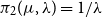
Table A.1. Inverse coverage probabilities from a simulation study of maximum likelihood and RHP predictions, using 100,000 training datasets each of a sample size of 20. The exponential, Pareto, and log-normal distribution predictions were calculated using exact expressions, while the Frećhet and Weibull predictions were calculated using the DMGS asymptotic approximation

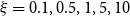
Table A.2. As Table A.1, but for a sample size of 50

B. Inverse Gamma Distribution Results

Figure B.1 As Figure 3, but now for the inverse gamma distribution.
C. Inverse Gaussian Distribution Results

Figure C.1 As Figure 3, but now for the inverse Gaussian distribution.
D. The fitdistcp software library
The calculations for this study were all performed using the fitdistcp software library, a free R library available on CRAN, developed by the first author, documented at https://fitdistcp.info. We now give some illustrative examples of fitdistcp commands:
-
• To evaluate maximum likelihood and RHP predictive densities for the exponential distribution, based on training data x, at locations y, the command is dexp_cp(x,y)
-
• To evaluate maximum likelihood and RHP predictive probabilities for the log-normal distribution, based on training data x, at locations y, the command is plnorm_cp(x,y).
-
• To evaluate maximum likelihood and RHP predictive quantiles for the Weibull distribution, based on training data x, at probabilities p, the command is qweibull_cp(x,p).
-
• To generate n maximum likelihood and calibrating prior predictive random deviates for the GPD with fixed location parameter, based on training data x, the command is rgpd_k1_cp(n,x).
Similar commands are available for a number of other commonly used distributions, including distributions with predictors on the parameters. Analytic solutions are used where possible. When analytic solutions are not available, the DMGS method is used, and ratio of uniforms sampling is also available as an option. Other options calculate model selection metrics, and additional routines are provided for evaluating reliability.
All fitdistcp commands can also be straightforwardly called from Python using the package rpy2, and the fitdistcp documentation provides an example of that.


 Open access