


1 Introduction and motivation
Tensor calculus is an essential tool in physics and applied mathematics. It was instrumental already a century ago in the formulation of Einstein’s general relativity, and its usage has spread to many areas of science. At its heart lies linear algebra, which is defined as the study of linear maps between vector spaces. In applications, one commonly manipulates representations of linear algebraic objects: vectors as 1-dimensional arrays and linear maps as matrices (2-dimensional arrays). Indeed, assuming a given basis, the representations are equivalent to the algebraic objects. Likewise, tensors are often thought of as a higher-dimensional version of matrices: their algebraic formulation is as a category of linear maps between vector spaces.
Viewing the above situation through the lens of programming language theory, the algebraic formulation forms a set of combinators and the array-based representations is a possible semantics for them. Even though the praxis is to blur the distinction between algebraic objects and their coefficient representations, it is a source of confusion in the case of tensor calculus, which studies tensor fields, in the sense of tensor-valued functions defined over a manifold. (We provide some evidence in Section 8.1.) Notably, difficulties arise because the basis varies over the manifold. The first contribution of this paper is to provide a clear conceptual picture by highlighting the syntax-semantics distinction.
On the practical side, the situation is similar. One can find a plethora of languages and libraries purportedly geared towards tensor manipulation, but they inevitably focus on their multi-dimensional array representations. There is nearly no support for algebraic tensor field expressions. In this paper, we work towards bridging this gap, by applying programming-language methodology to the notations of tensor algebra and tensor calculus—thus viewing them as domain-specific languages. For the readership with a programming language background, we aim to provide a down-to-earth presentation of tensor notations. We capture all their important properties, in particular by making use of linear types. We also aim to attract a readership that already has a working knowledge of tensors. For them we aim to fully formalise the relationship between the representation-oriented notation for tensor fields and its linear-algebraic semantics. We do so by viewing this syntax as terms in a (linear-typed) lambda calculus. As usual with dsls, this presentation comes with an executable semantics. This means we end up with a usable tool to manipulate tensor fields, which is the second contribution of this paper.
1.1 Overview
To make the presentation more pedagogical, we delay the introduction of tensor fields over manifolds until Section 5. Until then, the reader can think of each tensor as “just” an element of a certain vector space. This allows us to present the core concepts in a simpler setting, even though they will apply unchanged in the more general context. As hinted above, we will use an algebraic semantics for tensors, following a categorical structure (Section 3). Together, the combinators forming this categorical structure form a point-free edsl, which we refer to as Roger in reference to Roger Penrose (see Section 8.5 as for why).
Every Roger program can be evaluated to morphisms in any suitable tensor category. This includes matrices, but also string diagrams with the appropriate structure as well. Roger is useful in its own right, but has all the downsides of a point-free language, and thus is not in wide use in the mathematics community, where the so-called Einstein notation is preferred. The Einstein notation mimics the usual notation to access components of matrices, but speaks about these components in a wholesale manner, that is, with index variables that range over all the dimensions. We formalise this notation in an index-based edsl (Section 4). We refer to this edsl as Albert in the rest of the paper. Expressions in Albert evaluate to morphisms in Roger, and thus in any tensor category.
In sum, because the index-notation, diagram notation and matrices are instances of tensor categories, programs written in any of our edsls can be executed as tensor programs using the matrix instance or can generate index or diagram notation for the code in question. The relationships between these notations and edsls are depicted in Figure 1.

Fig. 1: Tensor notations, edsls and relationships between them. Even though the index notation, the morphism notation and the string diagram notation are all equivalent mathematically, in our implementation Roger is coded as a (set of) type-classes, and the index and diagram notations are instances of it.
This means that a function in Albert, say
will, depending on the type, either:
1. render itself in Einstein notation as $t{^i}\nabla{_i}u$
;
$t{^i}\nabla{_i}u$
;2. render itself as the diagram
or3. run on matrix representations of the tensors t and u and compute the result (a scalar field in this case, representing the directional derivative of u in the direction of t).

 or
orTogether, Albert and Roger form a Haskell library for expressing tensors.Footnote 1 This library leverages linear types as implemented in ghc 9. This implementation defines an executable semantics of Albert, and is presented in section 7. All the examples presented in this paper were prepared using our library. In particular, the diagrams are generated with it.
In Section 5, we move to deal with tensor fields proper. Essentially this means that every expression in either edsl corresponds to a tensor field, and that we can manipulate derivatives of such fields. With this addition, the edsls can be used for symbolic calculations of tensor fields. We can, for example, apply covariant derivatives to tensor expressions, re-express them in terms of partial derivatives and Christoffel symbols, and instantiate those to concrete coordinates systems. We demonstrate this workflow in Section 6, where we express Einstein’s General Relativity equation for the curvature of space-time and verify that the Schwarzschild metric tensor is a solution.
We start in Section 2 with a summary of the notions of linear algebra and tensors.
2 Background: linear algebra and tensors
The goal of this section is both to provide the canonical presentation as reference and to expose its abstruse character. The summary does not replace a proper introduction to the topic, and we urge the reader to turn to an appropriate reference if necessary (see references in Section 8.1).
A typical definition of tensor that one might find is the following:
An nth-rankFootnote 2 tensor in m-dimensional space is a mathematical object that has n indices and $m^n$
components and obeys certain transformation rules.
$m^n$
components and obeys certain transformation rules.
(Rowland & Weisstein, Reference Rowland and Weisstein2023)
(The transformations in question relate to change of basis, as we will see.) This kind of definition is heavily geared towards coordinate representations, rather than their algebraic definition. Why do pedagogical accounts widely refer to coordinate representations rather than semantics? One answer is that calculations are eventually always performed using coordinates. Another answer is that the kind of algebraic thinking required to grasp tensors may be too abstract to form an intuition. Our point of view is that it is indeed at the wrong abstraction level, and that the categorical structures are better suited to reasoning about tensors than the pure linear-algebraic ones. Nonetheless, we will have to refer to the algebraic definitions of tensors down the road, so we provide a minimal recap below.
2.1 Pure algebraic point of view
The main object of study are homomorphisms between vector spaces: linear transformations, also called linear maps. We will later see that tensors are such maps.
Definition 1 (vector space). A vector space (over a field S) is a commutative group $\mathsf{v}$
equipped with a compatible notion of scaling by elements of S.
$\mathsf{v}$
equipped with a compatible notion of scaling by elements of S.

A vector space must additionally satisfy a number of laws, including that scaling is a linear operation: $s \triangleleft (x+y) = s \triangleleft x+ s \triangleleft y$
.
$s \triangleleft (x+y) = s \triangleleft x+ s \triangleleft y$
.
The exact nature of this field of scalars (S) has little bearing on the algebraic developmentFootnote
3
, but we assume throughout that they are real numbers. Note that S is itself a vector space, with scaling ${(}\mskip 0.0mu\triangleleft \mskip 0.0mu{)}$
then being scalar multiplication.
${(}\mskip 0.0mu\triangleleft \mskip 0.0mu{)}$
then being scalar multiplication.
Definition 2 (linear map). A function $f: V \!\longrightarrow\! W$
is a linear map iff. for all collections of scalars
$f: V \!\longrightarrow\! W$
is a linear map iff. for all collections of scalars $c_{i}$
and vectors
$c_{i}$
and vectors $\vec v_{i}$
we have
$\vec v_{i}$
we have
 \begin{equation*}f \left(\sum _{i} c_{i} \triangleleft \vec v_{i}\right) = \sum _{i} c_{i} \triangleleft (f(\vec v_{i}))\end{equation*}
For a fixed domain and codomain, linear maps themselves form a vector space.

The eager reader should be warned that, for now, indices are used to range of over arbitrary sets of vectors and scalars (and bound by $\sum$
), in a usual way. Indices take a special meaning only when we get to coordinates and the Einstein notation (from Sections 2.2 and 2.3).
$\sum$
), in a usual way. Indices take a special meaning only when we get to coordinates and the Einstein notation (from Sections 2.2 and 2.3).
Definition 3 (covector space). Given a vector space V, the covector space $V^*$
is defined as the set of linear maps
$V^*$
is defined as the set of linear maps $V \!\longrightarrow\! S$
.
$V \!\longrightarrow\! S$
.
Since covector spaces are special cases of linear maps, they form vector spaces too. In a similar vein, the set of linear maps $f: S \!\longrightarrow\! W$
is isomorphic to W. (Indeed
$f: S \!\longrightarrow\! W$
is isomorphic to W. (Indeed $f(s) = f (s \triangleleft 1) = s \triangleleft f(1)$
, and thus the vector f(1) in W fully determines the linear function f.)
$f(s) = f (s \triangleleft 1) = s \triangleleft f(1)$
, and thus the vector f(1) in W fully determines the linear function f.)
Definition 4 (bilinear map). A function $f: V \times W \longrightarrow U$
is a bilinear map iff. for all
$f: V \times W \longrightarrow U$
is a bilinear map iff. for all $c_{i}, d_j : S$
,
$c_{i}, d_j : S$
, $\vec v_{i} : V$
, and
$\vec v_{i} : V$
, and $\vec w_j : W$
we have
$\vec w_j : W$
we have
 \begin{equation*}f \left(\sum _{i} c_{i} \triangleleft \vec v_{i}, \sum _j d_j \triangleleft \vec w_j\right) = \sum _{i,j} c_{i}d_j \triangleleft (f(\vec v_{i},\vec w_j))\end{equation*}
Definition 5 (Tensor product of vector spaces). Given two vector spaces V and W, their tensor product is a vector space, denoted by $V\otimes W$
, together with a bilinear map
$V\otimes W$
, together with a bilinear map $\phi:(V \times W) \!\longrightarrow\! (V\otimes W)$
with the following universal property. For every vector space Z and every bilinear map
$\phi:(V \times W) \!\longrightarrow\! (V\otimes W)$
with the following universal property. For every vector space Z and every bilinear map $h:(V \times W) \!\longrightarrow\! Z$
, there exists a unique linear map
$h:(V \times W) \!\longrightarrow\! Z$
, there exists a unique linear map $h' : (V\otimes W) \!\longrightarrow\! Z$
such that
$h' : (V\otimes W) \!\longrightarrow\! Z$
such that $h = h' \circ \phi$
. The output
$h = h' \circ \phi$
. The output $\phi(v,w)$
is often denoted by
$\phi(v,w)$
is often denoted by $v\otimes w$
, overloading the same symbol. (We let the reader check that the tensor product always exists.)
$v\otimes w$
, overloading the same symbol. (We let the reader check that the tensor product always exists.)
Examples: Here is an attempt at providing an intuition for what is, and is not, a bilinear function. Consider the simplest case of the definition of bilinear map where there is just one vector $\vec v$
as the first argument and one vector
$\vec v$
as the first argument and one vector $\vec w$
as the second argument to f. We then have
$\vec w$
as the second argument to f. We then have $f(\vec v,0) = f(1\triangleleft \vec v,0\triangleleft \vec w) = (1 \times 0)\triangleleft f(\vec v,\vec w) = 0$
. This means that vector addition is not bilinear because
$f(\vec v,0) = f(1\triangleleft \vec v,0\triangleleft \vec w) = (1 \times 0)\triangleleft f(\vec v,\vec w) = 0$
. This means that vector addition is not bilinear because $\vec v+0=\vec v \neq 0$
. Similarly, f cannot be first or second projection, because they are also linear, not bilinear.
$\vec v+0=\vec v \neq 0$
. Similarly, f cannot be first or second projection, because they are also linear, not bilinear.
We also have that we can “move constant factors” between $\vec v$
and
$\vec v$
and $\vec w$
:
$\vec w$
: $f(c \triangleleft \vec v, 1 \triangleleft \vec w) = (c \times 1) \triangleleft f(\vec v,\vec w) = (1 \times c) \triangleleft f(\vec v,\vec w) =f(1 \triangleleft \vec v, c \triangleleft \vec w)$
. In connection with the tensor product this means that even though, for any two vectors
$f(c \triangleleft \vec v, 1 \triangleleft \vec w) = (c \times 1) \triangleleft f(\vec v,\vec w) = (1 \times c) \triangleleft f(\vec v,\vec w) =f(1 \triangleleft \vec v, c \triangleleft \vec w)$
. In connection with the tensor product this means that even though, for any two vectors $\vec v : V$
and
$\vec v : V$
and $\vec w : W$
, we can construct a tensor
$\vec w : W$
, we can construct a tensor $u = \phi(\vec v,\vec w) : V\otimes W$
which looks like we have embedded a pair, we cannot extract
$u = \phi(\vec v,\vec w) : V\otimes W$
which looks like we have embedded a pair, we cannot extract $\vec v$
and
$\vec v$
and $\vec w$
again—they are mixed up together (entangled).
$\vec w$
again—they are mixed up together (entangled).
What a bilinear function can (and must) do, as we can see from the definition, when given two linear combinations, is to compute a linear combination based on all pairwise products of the coefficients, without depending on the coefficients themselves.
Order of a tensor
Often, tensors are used in a context where there is a single (atomic) underlying vector space $\mathsf{T}$
which is not just the scalars. Then the complexity of a vector space built from
$\mathsf{T}$
which is not just the scalars. Then the complexity of a vector space built from $\mathsf{T}$
can be measured by its order. The order of
$\mathsf{T}$
can be measured by its order. The order of $\mathsf{T}$
is defined to be 1 and the order of the scalar space is 0. The order of a tensor space
$\mathsf{T}$
is defined to be 1 and the order of the scalar space is 0. The order of a tensor space $\mathsf{V}\mskip 3.0mu{\otimes }\mskip 3.0mu\mathsf{W}$
is the sum of the order of spaces
$\mathsf{V}\mskip 3.0mu{\otimes }\mskip 3.0mu\mathsf{W}$
is the sum of the order of spaces $\mathsf{V}$
and
$\mathsf{V}$
and $\mathsf{W}$
, and this way we can build spaces of arbitrarily large order. The order of a linear map can be defined either as the pair of the orders of its input and output spaces, or as their sum (depending on convention). For example, a linear operator on an atomic vector space has order (1,1) or 2 in the respective conventions. Morphisms of order three or more are properly called tensors. Conversely, tensors of any order (including 0, 1 and 2) are linear maps, of the appropriate domain and codomain. When there is more that one underlying vector space, the order is not enough to characterise a tensor space: the full type needs to be specified, as in Section 3. (Yet this level of complexity won’t be exercised in this paper.)
$\mathsf{W}$
, and this way we can build spaces of arbitrarily large order. The order of a linear map can be defined either as the pair of the orders of its input and output spaces, or as their sum (depending on convention). For example, a linear operator on an atomic vector space has order (1,1) or 2 in the respective conventions. Morphisms of order three or more are properly called tensors. Conversely, tensors of any order (including 0, 1 and 2) are linear maps, of the appropriate domain and codomain. When there is more that one underlying vector space, the order is not enough to characterise a tensor space: the full type needs to be specified, as in Section 3. (Yet this level of complexity won’t be exercised in this paper.)
2.2 Coordinate representations
In practice, the algebraic definitions are not easy to manipulate for concrete problems, thus one most commonly works with coordinate representations instead. (Our goal will be to break free of those eventually.) As a reminder, given a basis $\vec e_{i}$
, any vector
$\vec e_{i}$
, any vector $\vec x\in V$
can be uniquely expressed as
$\vec x\in V$
can be uniquely expressed as $\vec x = \sum _{i} x^i\triangleleft \vec e_{i}$
where each
$\vec x = \sum _{i} x^i\triangleleft \vec e_{i}$
where each $x^i $
coordinate is a scalar. In this way, given a basis
$x^i $
coordinate is a scalar. In this way, given a basis $\vec e_{i}$
, a vector space is isomorphic to its set of coordinate representations. Note that a superscript is used for the index of such coordinates. The general convention that governs whether one should write indices in low or high positions is explained in Section 2.3; for now, it is enough to know that they are indexing notations.
$\vec e_{i}$
, a vector space is isomorphic to its set of coordinate representations. Note that a superscript is used for the index of such coordinates. The general convention that governs whether one should write indices in low or high positions is explained in Section 2.3; for now, it is enough to know that they are indexing notations.
Like vectors, linear maps are also commonly manipulated as matrices of coefficients. For a linear map f from a vector space with basis $\vec {d_{i}}$
to a space with basis
$\vec {d_{i}}$
to a space with basis $\vec e_j$
, each column is given by the coefficients of
$\vec e_j$
, each column is given by the coefficients of $f(\vec {d_{i}})$
. Indeed, using
$f(\vec {d_{i}})$
. Indeed, using $F{_i}{^j}$
to denote the coefficients, we have:
$F{_i}{^j}$
to denote the coefficients, we have:
 \begin{equation*} f(\vec x) = f\left(\sum _{i} x^i \triangleleft \vec {d_{i}}\right) = \sum _{i} x^i \triangleleft f(\vec {d_{i}}) = \sum _{i} x^i \triangleleft \left(\sum _j F{_i}{^j} \triangleleft \vec e_j\right) = \sum _j \left(\sum _i F{_i}{^j} x^i \right) \triangleleft \vec e_j\end{equation*}
In general, the values of the matrix coefficients $F{_i}{^j}$
depend on the choice of bases
$F{_i}{^j}$
depend on the choice of bases $\vec {d_{i}}$
and
$\vec {d_{i}}$
and $\vec e_j$
, but to reduce the number of moving parts one usually works with a coherent set of bases.
$\vec e_j$
, but to reduce the number of moving parts one usually works with a coherent set of bases.
Coherent bases
Starting from an atomic vector space T, one can build a collection of more complicated tensor spaces using tensor product, dual, and the unit (the scalar field S). For coordinate representations each such space could, in general, have its own basis, but it is standard to work with a collection of coherent bases. Given a basis $\vec e_{i}$
for a finite-dimensional atomic vector space T, the coherent basis for
$\vec e_{i}$
for a finite-dimensional atomic vector space T, the coherent basis for $T^*$
is the set of covectors
$T^*$
is the set of covectors $\tilde e^j$
such that
$\tilde e^j$
such that $\tilde e^j(\vec e_{i}) = \delta_{i}^j$
. (It is usually called the dual basis.) Likewise, given two coherent bases
$\tilde e^j(\vec e_{i}) = \delta_{i}^j$
. (It is usually called the dual basis.) Likewise, given two coherent bases $\vec {d_{i}}$
and
$\vec {d_{i}}$
and $\vec e_{i}$
respectively for V and W, the coherent basis for
$\vec e_{i}$
respectively for V and W, the coherent basis for $V\otimes W$
is
$V\otimes W$
is $b_{i,j} = \phi(\vec {d_{i}},\vec e_j)$
, where
$b_{i,j} = \phi(\vec {d_{i}},\vec e_j)$
, where $\phi$
is given by Definition 5. Note that this basis is indexed by a pair. Accordingly, if the dimension of V is m and the dimension of W is n, the dimension of
$\phi$
is given by Definition 5. Note that this basis is indexed by a pair. Accordingly, if the dimension of V is m and the dimension of W is n, the dimension of $V\otimes W$
is
$V\otimes W$
is $m \times n$
. Additionally, re-associating tensor spaces do not change coherent bases (
$m \times n$
. Additionally, re-associating tensor spaces do not change coherent bases ( $\vec e_{(i,j),k}$
is the same as
$\vec e_{(i,j),k}$
is the same as $\vec {d}_{i,(j,k)}$
, up to applying the corresponding associator). Finally, the scalar vector space has dimension one, and thus has a single base vector, which is coherently chosen to be the unit of the scalar field (the number
$\vec {d}_{i,(j,k)}$
, up to applying the corresponding associator). Finally, the scalar vector space has dimension one, and thus has a single base vector, which is coherently chosen to be the unit of the scalar field (the number $1 : S$
).
$1 : S$
).
Coordinate transformations
Assuming one basis $\vec e_j$
and another basis
$\vec e_j$
and another basis $\vec {d_{i}}$
for the same vector space V such that
$\vec {d_{i}}$
for the same vector space V such that $\vec {d_{i}} = \sum _j F{_i}{^j} \vec e_j$
, then the coordinates in basis
$\vec {d_{i}} = \sum _j F{_i}{^j} \vec e_j$
, then the coordinates in basis $\vec {d_{i}}$
for
$\vec {d_{i}}$
for $\vec x$
are
$\vec x$
are $\hat x^j = \sum _{i} F{_i}{^j} x^i $
. We say that the matrix F is the transformation matrix for V given the choice of bases made above, and denote it J(V). Then the transformation matrices for vector spaces built from an atomic space T using the coherent set of bases defined above are given by the following structural rules:
$\hat x^j = \sum _{i} F{_i}{^j} x^i $
. We say that the matrix F is the transformation matrix for V given the choice of bases made above, and denote it J(V). Then the transformation matrices for vector spaces built from an atomic space T using the coherent set of bases defined above are given by the following structural rules:
 \begin{align*}J(V\otimes W)&= J(V)\otimes J(W)&\text{Kronecker product of matrices}\\J(V^*)&= J(V)^{-1}&\text{matrix inverse}\\J(S)&= 1&\text{scalar unit}\end{align*}
Furthermore, the matrix representation G of a linear map $g : V \!\longrightarrow\! W$
is transformed to:
$g : V \!\longrightarrow\! W$
is transformed to: $J(W) \cdot G \cdot J(V^*)$
, where
$J(W) \cdot G \cdot J(V^*)$
, where $(\cdot)$
is matrix multiplication. These are the “transformation rules” that Rowland & Weisstein (Reference Rowland and Weisstein2023) allude to in the above quote.
$(\cdot)$
is matrix multiplication. These are the “transformation rules” that Rowland & Weisstein (Reference Rowland and Weisstein2023) allude to in the above quote.
2.3 Einstein notation
The previous section showed how to deal with concrete matrices, using a concrete choice of bases. The next step is to manipulate symbolic expressions involving matrices. The language of such expressions (together with a couple of simple conventions) is colloquially referred to as Einstein notation.
In this notation, every index ranges over the dimensions of an atomic vector space.Footnote 4 Consequently, the total number of free (non repeated) indices indicates the order of a tensor expression in index notation. An index can be written as a subscript (and called a low index) or as a superscript (and called a high index).
The location (high or low) of the index is dictated by which coordinate transformation applies to it. That is, if a high index ranges over the dimensions of V, then J(V) applies, whereas $J(V^*)$
applies for a low index. Additionally, every reference to a tensor is fully saturated, in the sense that a symbolic tensor is always applied to as many indices as its order. Thus, for instance,
$J(V^*)$
applies for a low index. Additionally, every reference to a tensor is fully saturated, in the sense that a symbolic tensor is always applied to as many indices as its order. Thus, for instance, $x^i$
denote (the components of) a vector, and
$x^i$
denote (the components of) a vector, and $y_j$
denote (the components of) a covector. The expression
$y_j$
denote (the components of) a covector. The expression $t{_i}{^j}$
refers to (components of) a linear transformation of order (1,1). In the absence of contraction (see below), multiplication increases the order of tensors. For instance,
$t{_i}{^j}$
refers to (components of) a linear transformation of order (1,1). In the absence of contraction (see below), multiplication increases the order of tensors. For instance, $x^i\,y_j$
also has order (1,1). In general, if t and u are expressions denoting tensors of order m and n, respectively, then their product
$x^i\,y_j$
also has order (1,1). In general, if t and u are expressions denoting tensors of order m and n, respectively, then their product $t\,u$
denotes a tensor of order
$t\,u$
denotes a tensor of order $m+n$
.
$m+n$
.
Contraction
In Einstein notation, the convention is that, within a term, a repeated index is implicitly summed over. (In terms familiar to this journal: such indices are implicitly bound by a summation operator.) Because summation is a linear operator, within a term all the well-scoped locations of the summation operator are equivalent—so it makes a lot of sense to omit them. Additionally, when an index is repeated, it must be repeated exactly twice; once as a high index and once as a low index. Mentioning an index twice is called contraction. Viewing tensors as higher dimensional matrices of coefficients, contraction consists in summing coefficients along a diagonal. Therefore, a contraction reduces the order of the tensor by two.Footnote
5
The indices which are contracted are sometimes called “dummy” and those that are not contracted are called “live” (In terms familiar to the functional programming community, dummies are bound variables and live indices are free variables.) To be well-scoped, every term in a sum must use the same live indices. For instance, the expression $t{_l}{^j}u{_m}{^k}v{_i}{^l}{^m} + v{_i}{^j}{^k}$
denotes a tensor of order (1,2). Its live indices are
$t{_l}{^j}u{_m}{^k}v{_i}{^l}{^m} + v{_i}{^j}{^k}$
denotes a tensor of order (1,2). Its live indices are ${}_i,{}^j,{}^k$
, and the indices m and l are dummies.
${}_i,{}^j,{}^k$
, and the indices m and l are dummies.
At this stage, one can see the Einstein notation as a convenient way to notate expressions which manipulate coordinates of tensors. The high/low index convention makes it clear which transformations apply. Yet it may be mysterious why indices must be repeated exactly twice, and why (live) indices cannot be omitted from a term. The answer lies in the following observation. Even though the Einstein notation may originate as a convenient way to express coordinates, it really is intended to describe algebraic objects. The physicists Thorne & Blandford (Reference Thorne and Blandford2015) put it this way:
[we suggest to] momentarily think of [Einstein notation] as a relationship between components of tensors in a specific basis; then do a quick mind-flip and regard it quite differently, as a relationship between geometric, basis-independent tensors with the
indices playing the roles of slot names.
(A “slot” is a component of input or output tensor space.) The key of this “mind flip” is that live indices correspond to inputs (or outputs) of linear functions, and contraction corresponds to connecting inputs to outputs. The main contribution of this paper is to work out this connection in full as a pair of two edsls.
3 Categorical structures
The key concepts needed to understand the essence of Einstein notation are the categorical structures that tensors inhabit. Besides, these structures will be instrumental in our design: we will let the user of Albert write expressions which are (close to) Einstein notation, but they will be evaluated to morphisms in the appropriate category. The underlying category can then be specialised according to the application at hand.
The categorical approach consists in raising the abstraction level, and focusing on the ways that linear maps are combined to construct more complex ones. The first step is to view linear maps as morphisms of a category whose objects are vector spaces. We render the type of morphisms from $\mathsf{a}$
to
$\mathsf{a}$
to $\mathsf{b}$
as
$\mathsf{b}$
as $\mathsf{a}\,\mskip 1.0mu\overset{z}{\leadsto }\mskip 1.0mu\,\mathsf{b}$
, corresponding to
$\mathsf{a}\,\mskip 1.0mu\overset{z}{\leadsto }\mskip 1.0mu\,\mathsf{b}$
, corresponding to $z\mskip 3.0mu\mathsf{a}\mskip 3.0mu\mathsf{b}$
in Haskell code.
$z\mskip 3.0mu\mathsf{a}\mskip 3.0mu\mathsf{b}$
in Haskell code.

Vector spaces form a commutative monoid under tensor product. Hence, linear maps form a symmetric monoidal category, or smc, whose combinators are as follows.

In the above smc class definition, we follow the usual convention of using the same symbol ${(}\mskip 0.0mu{\otimes }\mskip 0.0mu{)}$
both for the product of objects and the parallel composition of morphisms. In fact, this morphism operator is also called a tensor product in the literature. An smc comes with a number of laws, which are both unsurprising and extensively documented elsewhere (Barr & Wells, Reference Barr and Wells1999). We omit them here. The operations
${(}\mskip 0.0mu{\otimes }\mskip 0.0mu{)}$
both for the product of objects and the parallel composition of morphisms. In fact, this morphism operator is also called a tensor product in the literature. An smc comes with a number of laws, which are both unsurprising and extensively documented elsewhere (Barr & Wells, Reference Barr and Wells1999). We omit them here. The operations $\sigma $
(swap),
$\sigma $
(swap), $\alpha$
,
$\alpha$
, $\bar{\alpha}$
(associators) witness the commutative monoidal structure which tensor products possess. The unit of the tensor product, written
$\bar{\alpha}$
(associators) witness the commutative monoidal structure which tensor products possess. The unit of the tensor product, written $\mathbf{1}$
, is the scalar vector space (
$\mathbf{1}$
, is the scalar vector space ( $\mathsf{S}$
), which is witnessed by the isomorphisms
$\mathsf{S}$
), which is witnessed by the isomorphisms $\rho$
and
$\rho$
and $\bar{\rho}$
, called unitors.
$\bar{\rho}$
, called unitors.
As an example, take the morphism $\mathsf{ex}$
=
$\mathsf{ex}$
= ${(}\mskip 0.0mu\mathsf{id}\mskip 3.0mu{\otimes }\mskip 3.0mu\sigma \mskip 0.0mu{)}\mskip 3.0mu{\circ }\mskip 3.0mu\bar{\alpha}\mskip 3.0mu{\circ }\mskip 3.0mu{(}\mskip 0.0mu\mathsf{id}\mskip 3.0mu{\otimes }\mskip 3.0mu\alpha\mskip 3.0mu{\circ }\mskip 3.0mu{(}\mskip 0.0mu\sigma \mskip 3.0mu{\otimes }\mskip 3.0mu\mathsf{id}\mskip 0.0mu{)}\mskip 3.0mu{\circ }\mskip 3.0mu\bar{\alpha}\mskip 0.0mu{)}\mskip 3.0mu{\circ }\mskip 3.0mu\alpha\mskip 3.0mu{\circ }\mskip 3.0mu\alpha$
. It is polymorphic, but has in particular type
${(}\mskip 0.0mu\mathsf{id}\mskip 3.0mu{\otimes }\mskip 3.0mu\sigma \mskip 0.0mu{)}\mskip 3.0mu{\circ }\mskip 3.0mu\bar{\alpha}\mskip 3.0mu{\circ }\mskip 3.0mu{(}\mskip 0.0mu\mathsf{id}\mskip 3.0mu{\otimes }\mskip 3.0mu\alpha\mskip 3.0mu{\circ }\mskip 3.0mu{(}\mskip 0.0mu\sigma \mskip 3.0mu{\otimes }\mskip 3.0mu\mathsf{id}\mskip 0.0mu{)}\mskip 3.0mu{\circ }\mskip 3.0mu\bar{\alpha}\mskip 0.0mu{)}\mskip 3.0mu{\circ }\mskip 3.0mu\alpha\mskip 3.0mu{\circ }\mskip 3.0mu\alpha$
. It is polymorphic, but has in particular type ${(}\mskip 0.0mu{(}\mskip 0.0mu\mathsf{T}\mskip 3.0mu{\otimes }\mskip 3.0mu\mathsf{T}\mskip 0.0mu{)}\mskip 3.0mu{\otimes }\mskip 3.0mu\mathsf{T}\mskip 0.0mu{)}\mskip 3.0mu{\otimes }\mskip 3.0mu\mathsf{T}\,\mskip 1.0mu\overset{z}{\leadsto }\mskip 1.0mu\,{(}\mskip 0.0mu\mathsf{T}\mskip 3.0mu{\otimes }\mskip 3.0mu\mathsf{T}\mskip 0.0mu{)}\mskip 3.0mu{\otimes }\mskip 3.0mu{(}\mskip 0.0mu\mathsf{T}\mskip 3.0mu{\otimes }\mskip 3.0mu\mathsf{T}\mskip 0.0mu{)}$
. Its input and output orders are both 4, for a total order of (4,4) or 8. It is written
${(}\mskip 0.0mu{(}\mskip 0.0mu\mathsf{T}\mskip 3.0mu{\otimes }\mskip 3.0mu\mathsf{T}\mskip 0.0mu{)}\mskip 3.0mu{\otimes }\mskip 3.0mu\mathsf{T}\mskip 0.0mu{)}\mskip 3.0mu{\otimes }\mskip 3.0mu\mathsf{T}\,\mskip 1.0mu\overset{z}{\leadsto }\mskip 1.0mu\,{(}\mskip 0.0mu\mathsf{T}\mskip 3.0mu{\otimes }\mskip 3.0mu\mathsf{T}\mskip 0.0mu{)}\mskip 3.0mu{\otimes }\mskip 3.0mu{(}\mskip 0.0mu\mathsf{T}\mskip 3.0mu{\otimes }\mskip 3.0mu\mathsf{T}\mskip 0.0mu{)}$
. Its input and output orders are both 4, for a total order of (4,4) or 8. It is written $\delta{_i}{^m}\delta{_j}{^p}\delta{_k}{^n}\delta{_l}{^o}$
in Einstein notation, which makes more explicit the connection between inputs and output. An even more explicit notation is its rendering as a diagram:
$\delta{_i}{^m}\delta{_j}{^p}\delta{_k}{^n}\delta{_l}{^o}$
in Einstein notation, which makes more explicit the connection between inputs and output. An even more explicit notation is its rendering as a diagram:  .
.
This diagram notation can be generalised to all morphisms in a smc and is known as string diagrams. It is a two-dimensional instance of the abstract categorical structure. It is also fully abstract, in the sense that every diagram can be mapped to a unique morphism in the underlying smc. Figures 2 and 3 show several of the atomic diagrams which make up smcs. The guide for this notation is that each morphism is represented by a network of wires. Wires are drawn in a way that makes it clear which inputs are connected to which outputs. Because unit objects can be added and dropped at will (using $\rho$
and
$\rho$
and $\bar{\rho}$
), under some conventions the corresponding wires are not drawn at all. Here we choose to draw them as grey lines.
$\bar{\rho}$
), under some conventions the corresponding wires are not drawn at all. Here we choose to draw them as grey lines.

Fig. 2: Diagram, categorical and index notations for identity and composition.

Fig. 3: Diagram, categorical, and Einstein notations for morphisms of symmetric monoidal categories. They are in general polymorphic, but we display them here as acting on an atomic vector space T, or the simplest allowable combination thereof (see the last row in the figure for the monomorphic type of the respective morphisms). The morphisms $\bar{\alpha}$
and
$\bar{\alpha}$
and $\bar{\rho}$
are not shown, but are drawn symmetrically to
$\bar{\rho}$
are not shown, but are drawn symmetrically to $\alpha$
and
$\alpha$
and $\rho$
, respectively.
$\rho$
, respectively.
The diagram notation is defined in such a way that morphisms that are equal under the category laws have topologically equivalent diagram representations (Selinger, Reference Selinger2011). That is, if we can deform one diagram to another without cutting wires, then they are equivalent. We can illustrate this kind of topological reasoning with the following simple example. Assuming an abstract tensor $\mathsf{u}\mskip 3.0mu{:}\mskip 3.0mu\mathsf{T}\,\mskip 1.0mu\overset{z}{\leadsto }\mskip 1.0mu\,\mathsf{T}$
, one can check that
$\mathsf{u}\mskip 3.0mu{:}\mskip 3.0mu\mathsf{T}\,\mskip 1.0mu\overset{z}{\leadsto }\mskip 1.0mu\,\mathsf{T}$
, one can check that $\sigma \mskip 3.0mu{\circ }\mskip 3.0mu{(}\mskip 0.0mu\mathsf{id}\mskip 3.0mu{\otimes }\mskip 3.0mu\mathsf{u}\mskip 0.0mu{)}\mskip 3.0mu{\circ }\mskip 3.0mu\sigma \mskip 3.0mu{\circ }\mskip 3.0mu{(}\mskip 0.0mu\mathsf{id}\mskip 3.0mu{\otimes }\mskip 3.0mu\mathsf{u}\mskip 0.0mu{)}$
is equivalent to
$\sigma \mskip 3.0mu{\circ }\mskip 3.0mu{(}\mskip 0.0mu\mathsf{id}\mskip 3.0mu{\otimes }\mskip 3.0mu\mathsf{u}\mskip 0.0mu{)}\mskip 3.0mu{\circ }\mskip 3.0mu\sigma \mskip 3.0mu{\circ }\mskip 3.0mu{(}\mskip 0.0mu\mathsf{id}\mskip 3.0mu{\otimes }\mskip 3.0mu\mathsf{u}\mskip 0.0mu{)}$
is equivalent to $\mathsf{u}\mskip 3.0mu{\otimes }\mskip 3.0mu\mathsf{u}$
by applying a number of algebraic laws, but this is an error-prone process. If we first convert the morphisms to diagram form, we need to check
$\mathsf{u}\mskip 3.0mu{\otimes }\mskip 3.0mu\mathsf{u}$
by applying a number of algebraic laws, but this is an error-prone process. If we first convert the morphisms to diagram form, we need to check ![]() which is a matter of repositioning the second box.Footnote 6
which is a matter of repositioning the second box.Footnote 6
At this point, a reader familiar with programming languages might be tempted to assume that $\mathsf{V}\mskip 3.0mu{\otimes }\mskip 3.0mu\mathsf{W}$
is like a pair of
$\mathsf{V}\mskip 3.0mu{\otimes }\mskip 3.0mu\mathsf{W}$
is like a pair of $\mathsf{V}$
and
$\mathsf{V}$
and $\mathsf{W}$
. That is, that tensors would not only form a category, but even a Cartesian category. This is not the case: tensors are not equipped with projections nor duplications. This observation justifies the fact that contraction in Einstein notation must involve exactly two indices. Indeed, contraction corresponds to connecting loose wires in the diagram notation, and because we do not have a Cartesian category, only two loose wires can be connected (to make a new continuous wire).
$\mathsf{W}$
. That is, that tensors would not only form a category, but even a Cartesian category. This is not the case: tensors are not equipped with projections nor duplications. This observation justifies the fact that contraction in Einstein notation must involve exactly two indices. Indeed, contraction corresponds to connecting loose wires in the diagram notation, and because we do not have a Cartesian category, only two loose wires can be connected (to make a new continuous wire).
Addition and scaling
As we saw, tensors of the same type (same domain and codomain) form themselves a vector space, and as such can be scaled and added together. The corresponding categorical structure is called an additive category. Thus, every tensor category z will satisfy the $\mathsf{Additive}$
constraint:
$\mathsf{Additive}$
constraint:
Recalling the definition of $\mathsf{VectorSpace}$
from Section 2.1,
$\mathsf{VectorSpace}$
from Section 2.1, $\mathsf{Additive}$
implies that we have the following two operations for every
$\mathsf{Additive}$
implies that we have the following two operations for every $\mathsf{a}$
and
$\mathsf{a}$
and $\mathsf{b}$
:
$\mathsf{b}$
:

An additive category requires that composition ${(}\mskip 0.0mu{\circ }\mskip 0.0mu{)}$
and tensor products
${(}\mskip 0.0mu{\circ }\mskip 0.0mu{)}$
and tensor products ${(}\mskip 0.0mu{\otimes }\mskip 0.0mu{)}$
are bilinear. In full:
${(}\mskip 0.0mu{\otimes }\mskip 0.0mu{)}$
are bilinear. In full:

We note in passing that there is no obviously good way to represent addition using diagrams. If diagrams should be added together we write them side by side with a plus sign in between.
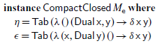
Compact Closed Category There remains to capture the relationship between a vector space V and its associated covector space $V^*$
. This is done abstractly using a compact closed category structure (Selinger, Reference Selinger2011). In a compact closed category, every object has a dual, and duals generalise the notion of co-vector space.
$V^*$
. This is done abstractly using a compact closed category structure (Selinger, Reference Selinger2011). In a compact closed category, every object has a dual, and duals generalise the notion of co-vector space.

In the tensor instance, $\eta$
and
$\eta$
and $\epsilon$
produce and consume correlated products of vectors and covectors. While the algebraic view is very abstract and can be hard to grasp (it is for the authors), the diagrams help. Compact closed categories are required to satisfy the so-called snake laws: one is
$\epsilon$
produce and consume correlated products of vectors and covectors. While the algebraic view is very abstract and can be hard to grasp (it is for the authors), the diagrams help. Compact closed categories are required to satisfy the so-called snake laws: one is ${(}\mskip 0.0mu\epsilon\mskip 3.0mu{\otimes }\mskip 3.0mu\mathsf{id}\mskip 0.0mu{)}\mskip 3.0mu{\circ }\mskip 3.0mu\bar{\alpha}\mskip 3.0mu{\circ }\mskip 3.0mu{(}\mskip 0.0mu\mathsf{id}\mskip 3.0mu{\otimes }\mskip 3.0mu\eta\mskip 0.0mu{)}$
=
${(}\mskip 0.0mu\epsilon\mskip 3.0mu{\otimes }\mskip 3.0mu\mathsf{id}\mskip 0.0mu{)}\mskip 3.0mu{\circ }\mskip 3.0mu\bar{\alpha}\mskip 3.0mu{\circ }\mskip 3.0mu{(}\mskip 0.0mu\mathsf{id}\mskip 3.0mu{\otimes }\mskip 3.0mu\eta\mskip 0.0mu{)}$
= $\sigma $
, or
$\sigma $
, or ![]() , and the other is symmetrical. These laws ensure that the object
, and the other is symmetrical. These laws ensure that the object ${\mathsf{a}^*}$
is just like the object
${\mathsf{a}^*}$
is just like the object $\mathsf{a}$
, but travelling backwards (input and output roles are exchanged). To reflect this, in the diagrammatic representation of
$\mathsf{a}$
, but travelling backwards (input and output roles are exchanged). To reflect this, in the diagrammatic representation of $\eta$
and
$\eta$
and $\epsilon$
, we indicate the
$\epsilon$
, we indicate the ${\mathsf{a}^*}$
object with a left-pointing arrow, as shown in Figure 4(a). Indeed, there is no difference between an input vector space
${\mathsf{a}^*}$
object with a left-pointing arrow, as shown in Figure 4(a). Indeed, there is no difference between an input vector space $\mathsf{a}$
and an output vector space
$\mathsf{a}$
and an output vector space ${\mathsf{a}^*}$
. Accordingly, in the Einstein notation, no difference is being made between inputs and outputs. Instead only co- or contra-variance is reflected notationally. Consequently neither
${\mathsf{a}^*}$
. Accordingly, in the Einstein notation, no difference is being made between inputs and outputs. Instead only co- or contra-variance is reflected notationally. Consequently neither $\eta$
nor
$\eta$
nor $\epsilon$
are visible in the Einstein notation, except perhaps as a Kronecker
$\epsilon$
are visible in the Einstein notation, except perhaps as a Kronecker $\delta$
(see Figure 4(a)). For instance, the morphism
$\delta$
(see Figure 4(a)). For instance, the morphism $\epsilon\mskip 3.0mu{\circ }\mskip 3.0mu{(}\mskip 0.0mu\bar{\rho}\mskip 3.0mu{\circ }\mskip 3.0mu{(}\mskip 0.0mu\mathsf{id}\mskip 3.0mu{\otimes }\mskip 3.0mu\epsilon\mskip 0.0mu{)}\mskip 3.0mu{\otimes }\mskip 3.0mu\mathsf{id}\mskip 0.0mu{)}\mskip 3.0mu{\circ }\mskip 3.0mu{(}\mskip 0.0mu\alpha\mskip 3.0mu{\otimes }\mskip 3.0mu\mathsf{id}\mskip 0.0mu{)}\mskip 3.0mu{\circ }\mskip 3.0mu{(}\mskip 0.0mu{(}\mskip 0.0mu\sigma \mskip 3.0mu{\otimes }\mskip 3.0mu\mathsf{id}\mskip 0.0mu{)}\mskip 3.0mu{\otimes }\mskip 3.0mu\mathsf{id}\mskip 0.0mu{)}$
, or
$\epsilon\mskip 3.0mu{\circ }\mskip 3.0mu{(}\mskip 0.0mu\bar{\rho}\mskip 3.0mu{\circ }\mskip 3.0mu{(}\mskip 0.0mu\mathsf{id}\mskip 3.0mu{\otimes }\mskip 3.0mu\epsilon\mskip 0.0mu{)}\mskip 3.0mu{\otimes }\mskip 3.0mu\mathsf{id}\mskip 0.0mu{)}\mskip 3.0mu{\circ }\mskip 3.0mu{(}\mskip 0.0mu\alpha\mskip 3.0mu{\otimes }\mskip 3.0mu\mathsf{id}\mskip 0.0mu{)}\mskip 3.0mu{\circ }\mskip 3.0mu{(}\mskip 0.0mu{(}\mskip 0.0mu\sigma \mskip 3.0mu{\otimes }\mskip 3.0mu\mathsf{id}\mskip 0.0mu{)}\mskip 3.0mu{\otimes }\mskip 3.0mu\mathsf{id}\mskip 0.0mu{)}$
, or  in diagram notation, is written $\delta{_i}{^k}\delta{_j}{^l}$
in Einstein notation. Figure 4(b) shows how an input object
$\delta{_i}{^k}\delta{_j}{^l}$
in Einstein notation. Figure 4(b) shows how an input object $\mathsf{a}$
(of any morphism) can be converted to an output
$\mathsf{a}$
(of any morphism) can be converted to an output ${\mathsf{a}^*}$
, and vice versa. One can even combine both ideas and connect the output of a morphism
${\mathsf{a}^*}$
, and vice versa. One can even combine both ideas and connect the output of a morphism $\mathsf{t}$
back to its input. By doing so, one constructs the trace of
$\mathsf{t}$
back to its input. By doing so, one constructs the trace of $\mathsf{t}$
.Footnote 7
$\mathsf{t}$
.Footnote 7

Fig. 4: Illustration of compact closed categories in various notations. Note that Einstein notation does not change when bending connections using $\eta$
or
$\eta$
or $\epsilon$
, though in the third example, the new connection is notated by repeated use of the index.
$\epsilon$
, though in the third example, the new connection is notated by repeated use of the index.
We now have a complete description of the tensor combinators—the core of Roger. Unfortunately, in practice, it is inconvenient to use as such. Indeed, most of the tensor expressions encountered in practice consists of building a network of connections between atomic blocks. Unfortunately, using the categorical combinators for this purpose is tedious. For instance, contracting two input indices is particularly tedious in the point-free notation, because it is realised as a composition with $\eta$
or
$\eta$
or $\epsilon$
with a large number of smc combinators to select the appropriate dimensions to contract. It is akin to programming with SKI combinators instead of using the lambda calculus. Using variable names for indices, like in the Einstein notation, would be much more convenient. We will get there in Section 4.
$\epsilon$
with a large number of smc combinators to select the appropriate dimensions to contract. It is akin to programming with SKI combinators instead of using the lambda calculus. Using variable names for indices, like in the Einstein notation, would be much more convenient. We will get there in Section 4.
3.1 Matrix instances
An important instance of the compact closed category structure is the category of matrices of coefficients, which we encountered in Section 2.2. In our host functional language, we define them as a function from (both input and output) indices to coefficients (of type $\mathsf{S}$
):Footnote
8
$\mathsf{S}$
):Footnote
8
To emphasise the dependency on the basis, we use a subscript when referring to a specific matrix category morphism, as in $M_{\mathsf{b}}$
where
$M_{\mathsf{b}}$
where $\mathsf{b}$
is a reference to the choice of basis. In the Haskell implementation, this basis is represented by a phantom type parameter.
$\mathsf{b}$
is a reference to the choice of basis. In the Haskell implementation, this basis is represented by a phantom type parameter.
The identity morphism is the identity matrix, and composition is matrix multiplication:

In this instance, the objects are identified with sets that index the bases of the vector spaces that they stand for. These sets are assumed to be enumerable and bounded (so we have access to their $\mathsf{inhabitants}$
) and we can compare indices for equality.Footnote 9 The instance of the smc structure for matrix representations in coherent bases is then:
$\mathsf{inhabitants}$
) and we can compare indices for equality.Footnote 9 The instance of the smc structure for matrix representations in coherent bases is then:

Because objects index the bases of the corresponding vector spaces, tensor products are represented as usual pairs. In the above definition, the right-hand sides are Haskell code. This means that the asterisk operator ${(}\mskip 0.0mu{*}\mskip 0.0mu{)}$
denotes multiplication between scalars as components of matrices. In contrast, the operator
${(}\mskip 0.0mu{*}\mskip 0.0mu{)}$
denotes multiplication between scalars as components of matrices. In contrast, the operator $(\star)$
defined in Section 4 denotes multiplication between abstract scalar (order-0) tensor expressions (independent of the chosen tensor representation).
$(\star)$
defined in Section 4 denotes multiplication between abstract scalar (order-0) tensor expressions (independent of the chosen tensor representation).
With the coherent choice of bases, $\eta$
and
$\eta$
and $\epsilon$
are simply realised as the identity.
$\epsilon$
are simply realised as the identity.
The object ${\mathsf{a}^*}$
has the same dimensionality as
${\mathsf{a}^*}$
has the same dimensionality as $\mathsf{a}$
, so in our Haskell encoding we use
$\mathsf{a}$
, so in our Haskell encoding we use $\mathbf{newtype}$
for it,
$\mathbf{newtype}$
for it, ![]() . For concision (and following tradition), we use an asterisk as a shorthand, so
. For concision (and following tradition), we use an asterisk as a shorthand, so ${\mathsf{a}^*}$
stands for the type
${\mathsf{a}^*}$
stands for the type $\mathsf{DualObject}\mskip 3.0mu\mathsf{a}$
.
$\mathsf{DualObject}\mskip 3.0mu\mathsf{a}$
.
Coordinate representation functors. It is worth mentioning that the transformation functions between linear maps $\mathsf{L}$
and their representations
$\mathsf{L}$
and their representations $M_{\mathsf{e}}$
in a given basis
$M_{\mathsf{e}}$
in a given basis $\mathsf{e}$
are a pair of functors which are the identity on objects and just change the morphisms:
$\mathsf{e}$
are a pair of functors which are the identity on objects and just change the morphisms:
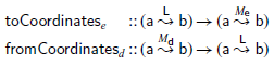
Furthermore, this pair defines an isomorphism between the respective compact-closed categories. Therefore, even though different representations form different categories, one can always transform one to another. The transformation between systems of coordinates, usually presented using transformation matrices (see Section 2.2) can be understood as the composition of $\mathsf{fromCoordinates}$
in the source basis, and
$\mathsf{fromCoordinates}$
in the source basis, and $\mathsf{toCoordinates}$
in the target basis:
$\mathsf{toCoordinates}$
in the target basis:

4 Design of
${\mathbf{A}\scriptstyle \mathbf{LBERT}}$

In this section, we provide the design of Albert. We intend our design to match Einstein notation as closely as possible. This aim is achieved except for the following two differences:
1. Indices can range over the dimensions of any space (not just atomic vector spacesFootnote 10 )
2. Indices are always explicitly bound
The first difference is motivated by polymorphism considerations: we make many functions polymorphic over the vector space that they manipulate, and as a consequence, the corresponding indices can range over the dimensions of tensor or scalar vector spaces. For instance, when we write $\mathsf{delta}\mskip 3.0mu_{\mathsf{i}}\mskip 3.0mu^{\mathsf{j}}$
, indices (
$\mathsf{delta}\mskip 3.0mu_{\mathsf{i}}\mskip 3.0mu^{\mathsf{j}}$
, indices ( $_{\mathsf{i}}$
,
$_{\mathsf{i}}$
, $^{\mathsf{j}}$
) may range over order-2 tensor spaces, in which case the corresponding Einstein notation would be the product of two Kronecker deltas.
$^{\mathsf{j}}$
) may range over order-2 tensor spaces, in which case the corresponding Einstein notation would be the product of two Kronecker deltas.
The second difference is motivated by the need to follow the functional programming conventions, which is required to embed the dsl in Haskell, or any functional language without macros. Besides, to avoid confusion, in Albert we choose names in all letters for combinators. For instance, when the conventional notation is the Greek letter $\delta$
, we write
$\delta$
, we write $\mathsf{delta}$
in Albert.
$\mathsf{delta}$
in Albert.
The principles and most of the interface of Albert are presented in this section. The tensor-field specific functions are discussed in Section 5. The complete interface is summarised in Figures 9 and 10.

Fig. 9: Syntax of the index language of Albert, as types of combinators.

Fig. 10: Syntax of the expression sub-language of Albert, as types of combinators. We repeat christoffel symbol and metric here even though they can be defined by the user as the embedding of the corresponding Roger primitives.
Types All types are parameterised by z, the category which tensors inhabit. The type of an index ranging over the dimensions of vector space $\mathsf{a}$
is
$\mathsf{a}$
is $\mathsf{P}\mskip 3.0muz\mskip 3.0mu\mathsf{r}\mskip 3.0mu\mathsf{a}$
(think of
$\mathsf{P}\mskip 3.0muz\mskip 3.0mu\mathsf{r}\mskip 3.0mu\mathsf{a}$
(think of $\mathsf{P}$
as “port” or “end of a wire carrying
$\mathsf{P}$
as “port” or “end of a wire carrying $\mathsf{a}$
” in the diagrams), where the variable
$\mathsf{a}$
” in the diagrams), where the variable $\mathsf{r}$
is a technical (scoping) device (made precise in Section 7). For the purpose of using Albert, it suffices to know that this variable
$\mathsf{r}$
is a technical (scoping) device (made precise in Section 7). For the purpose of using Albert, it suffices to know that this variable $\mathsf{r}$
should be consistent throughout any given expression.
$\mathsf{r}$
should be consistent throughout any given expression.
The type of expressions is $\mathsf{R}\mskip 3.0muz\mskip 3.0mu\mathsf{r}$
. Expressions of this type closely match expressions in Einstein notation. In particular, expressions with several free index variables correspond to higher-order tensors. For example, assuming two free index variables
$\mathsf{R}\mskip 3.0muz\mskip 3.0mu\mathsf{r}$
. Expressions of this type closely match expressions in Einstein notation. In particular, expressions with several free index variables correspond to higher-order tensors. For example, assuming two free index variables $_{\mathsf{i}}\mskip 3.0mu{::}\mskip 3.0mu\mathsf{P}\mskip 3.0muz\mskip 3.0mu\mathsf{r}\mskip 3.0mu\mathsf{T}$
and
$_{\mathsf{i}}\mskip 3.0mu{::}\mskip 3.0mu\mathsf{P}\mskip 3.0muz\mskip 3.0mu\mathsf{r}\mskip 3.0mu\mathsf{T}$
and $^{\mathsf{j}}\mskip 3.0mu{::}\mskip 3.0mu\mathsf{P}\mskip 3.0muz\mskip 3.0mu\mathsf{r}\mskip 3.0mu{\mathsf{T}^*}$
, then
$^{\mathsf{j}}\mskip 3.0mu{::}\mskip 3.0mu\mathsf{P}\mskip 3.0muz\mskip 3.0mu\mathsf{r}\mskip 3.0mu{\mathsf{T}^*}$
, then $\mathsf{w}\mskip 3.0mu_{\mathsf{i}}\mskip 3.0mu{::}\mskip 3.0mu\mathsf{R}\mskip 3.0muz\mskip 3.0mu\mathsf{r}$
represents a covector over
$\mathsf{w}\mskip 3.0mu_{\mathsf{i}}\mskip 3.0mu{::}\mskip 3.0mu\mathsf{R}\mskip 3.0muz\mskip 3.0mu\mathsf{r}$
represents a covector over $\mathsf{T}$
;
$\mathsf{T}$
; $\mathsf{v}\mskip 3.0mu^{\mathsf{j}}\mskip 3.0mu{::}\mskip 3.0mu\mathsf{R}\mskip 3.0muz\mskip 3.0mu\mathsf{r}$
represents a vector in
$\mathsf{v}\mskip 3.0mu^{\mathsf{j}}\mskip 3.0mu{::}\mskip 3.0mu\mathsf{R}\mskip 3.0muz\mskip 3.0mu\mathsf{r}$
represents a vector in $\mathsf{T}$
; and
$\mathsf{T}$
; and $\mathsf{t}\mskip 3.0mu_{\mathsf{i}}\mskip 3.0mu^{\mathsf{j}}\mskip 3.0mu{::}\mskip 3.0mu\mathsf{R}\mskip 3.0muz\mskip 3.0mu\mathsf{r}$
represents a linear map from
$\mathsf{t}\mskip 3.0mu_{\mathsf{i}}\mskip 3.0mu^{\mathsf{j}}\mskip 3.0mu{::}\mskip 3.0mu\mathsf{R}\mskip 3.0muz\mskip 3.0mu\mathsf{r}$
represents a linear map from $\mathsf{T}$
to
$\mathsf{T}$
to $\mathsf{T}$
. (Why this is so will become clear when we present the semantics of tensors, which we will do before the end of the section.)
$\mathsf{T}$
. (Why this is so will become clear when we present the semantics of tensors, which we will do before the end of the section.)
In sum, exactly as in Einstein notation, our tensor expressions define and manipulate tensors as (abstract) scalar-valued expressions depending on indices. Likewise, the order of the underlying tensor is the sum of the order of the free index variables occurring in it. Even though we present index variables as either super- or subscripts, they are just regular variable names.
Because the underlying category z is not Cartesian, every input must be connected to a single output, and vice-versa. Hence, index variables occur exactly once in each term. We enforce this restriction by using (and binding) index variables linearly.Footnote
11
Accordingly, the types of the variables $\mathsf{v}\mskip 0.0mu{,}\mskip 3.0mu\mathsf{w}\mskip 0.0mu{,}\mskip 3.0mu\mathsf{t}$
mentioned above involve (type-)linear functions. For instance
$\mathsf{v}\mskip 0.0mu{,}\mskip 3.0mu\mathsf{w}\mskip 0.0mu{,}\mskip 3.0mu\mathsf{t}$
mentioned above involve (type-)linear functions. For instance $\mathsf{w}\mskip 3.0mu{::}\mskip 3.0mu\mathsf{P}\mskip 3.0muz\mskip 3.0mu\mathsf{r}\mskip 3.0mu\mathsf{T}\mskip 3.0mu{\multimap }\mskip 3.0mu\mathsf{R}\mskip 3.0muz\mskip 3.0mu\mathsf{r}$
is a covector over
$\mathsf{w}\mskip 3.0mu{::}\mskip 3.0mu\mathsf{P}\mskip 3.0muz\mskip 3.0mu\mathsf{r}\mskip 3.0mu\mathsf{T}\mskip 3.0mu{\multimap }\mskip 3.0mu\mathsf{R}\mskip 3.0muz\mskip 3.0mu\mathsf{r}$
is a covector over $\mathsf{T}$
;
$\mathsf{T}$
; $\mathsf{v}\mskip 3.0mu{::}\mskip 3.0mu\mathsf{P}\mskip 3.0muz\mskip 3.0mu\mathsf{r}\mskip 3.0mu{\mathsf{T}^*}\mskip 3.0mu{\multimap }\mskip 3.0mu\mathsf{R}\mskip 3.0muz\mskip 3.0mu\mathsf{r}$
is a vector in
$\mathsf{v}\mskip 3.0mu{::}\mskip 3.0mu\mathsf{P}\mskip 3.0muz\mskip 3.0mu\mathsf{r}\mskip 3.0mu{\mathsf{T}^*}\mskip 3.0mu{\multimap }\mskip 3.0mu\mathsf{R}\mskip 3.0muz\mskip 3.0mu\mathsf{r}$
is a vector in $\mathsf{T}$
; and
$\mathsf{T}$
; and $\mathsf{t}\mskip 3.0mu{::}\mskip 3.0mu\mathsf{P}\mskip 3.0muz\mskip 3.0mu\mathsf{r}\mskip 3.0mu\mathsf{T}\mskip 3.0mu{\multimap }\mskip 3.0mu\mathsf{P}\mskip 3.0muz\mskip 3.0mu\mathsf{r}\mskip 3.0mu{\mathsf{T}^*}\mskip 3.0mu{\multimap }\mskip 3.0mu\mathsf{R}\mskip 3.0muz\mskip 3.0mu\mathsf{r}$
is a linear map over
$\mathsf{t}\mskip 3.0mu{::}\mskip 3.0mu\mathsf{P}\mskip 3.0muz\mskip 3.0mu\mathsf{r}\mskip 3.0mu\mathsf{T}\mskip 3.0mu{\multimap }\mskip 3.0mu\mathsf{P}\mskip 3.0muz\mskip 3.0mu\mathsf{r}\mskip 3.0mu{\mathsf{T}^*}\mskip 3.0mu{\multimap }\mskip 3.0mu\mathsf{R}\mskip 3.0muz\mskip 3.0mu\mathsf{r}$
is a linear map over $\mathsf{T}$
. This means that Albert uses a higher-order abstract syntax, that is, the abstraction mechanism of the host language provides us with the means to abstract over index variables. The order of a tensor variable is given by taking the sum of the order of the index parameters in its type. So, for instance,
$\mathsf{T}$
. This means that Albert uses a higher-order abstract syntax, that is, the abstraction mechanism of the host language provides us with the means to abstract over index variables. The order of a tensor variable is given by taking the sum of the order of the index parameters in its type. So, for instance, $\mathsf{delta}$
has order 2m if its type argument
$\mathsf{delta}$
has order 2m if its type argument $\mathsf{a}$
stands for a vector space of order m:
$\mathsf{a}$
stands for a vector space of order m:
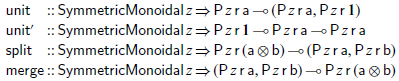
Tensor embedding, evaluation, and index manipulation Next, we turn our attention to embedding Roger into Albert. This is done by means of the following combinators:
The special case of a vector, where the target object is the unit, is common enough that it deserves a function of its own. In the general case, we take advantage of the compact-closed structure, and turn the output object ( $\mathsf{b}$
) of the morphism into an input of an index over the dual object (
$\mathsf{b}$
) of the morphism into an input of an index over the dual object ( ${\mathsf{b}^*}$
).
${\mathsf{b}^*}$
).
The converse operation consists in evaluating a tensor expression into a morphism:

The fact that we can move between these two dsls freely (using embedding and evaluation) means we can combine their strengths. In both embedding and evaluation, neither $\mathsf{a}$
nor
$\mathsf{a}$
nor $\mathsf{b}$
need be atomic types. To match the convention of Einstein notation, the user of Albert can break down the corresponding indices into their components after embedding, or conversely combine components before evaluation. Likewise, unit objects might need to be introduced or discarded. The interface for performing such operations is provided in the form of the following four combinators:
$\mathsf{b}$
need be atomic types. To match the convention of Einstein notation, the user of Albert can break down the corresponding indices into their components after embedding, or conversely combine components before evaluation. Likewise, unit objects might need to be introduced or discarded. The interface for performing such operations is provided in the form of the following four combinators:
To sum up, when z is a smc, the $\mathsf{P}\mskip 3.0muz\mskip 3.0mu\mathsf{r}$
type transformer defines a homomorphism between the monoid of (linear) Haskell pairs and that of tensor products of the category z. As an illustration, a function
$\mathsf{P}\mskip 3.0muz\mskip 3.0mu\mathsf{r}$
type transformer defines a homomorphism between the monoid of (linear) Haskell pairs and that of tensor products of the category z. As an illustration, a function $\mathsf{t}$
of type
$\mathsf{t}$
of type $\mathsf{P}\mskip 3.0muz\mskip 3.0mu\mathsf{r}\mskip 3.0mu{(}\mskip 0.0mu\mathsf{a}\mskip 3.0mu{\otimes }\mskip 3.0mu{\mathsf{b}^*}\mskip 0.0mu{)}\mskip 3.0mu{\multimap }\mskip 3.0mu\mathsf{R}\mskip 3.0muz\mskip 3.0mu\mathsf{r}$
can be curried to
$\mathsf{P}\mskip 3.0muz\mskip 3.0mu\mathsf{r}\mskip 3.0mu{(}\mskip 0.0mu\mathsf{a}\mskip 3.0mu{\otimes }\mskip 3.0mu{\mathsf{b}^*}\mskip 0.0mu{)}\mskip 3.0mu{\multimap }\mskip 3.0mu\mathsf{R}\mskip 3.0muz\mskip 3.0mu\mathsf{r}$
can be curried to $\mathsf{t'}\mskip 3.0mu{::}\mskip 3.0mu\mathsf{P}\mskip 3.0muz\mskip 3.0mu\mathsf{r}\mskip 3.0mu\mathsf{a}\mskip 3.0mu{\multimap }\mskip 3.0mu\mathsf{P}\mskip 3.0muz\mskip 3.0mu\mathsf{r}\mskip 3.0mu{\mathsf{b}^*}\mskip 3.0mu{\multimap }\mskip 3.0mu\mathsf{R}\mskip 3.0muz\mskip 3.0mu\mathsf{r}$
. When using
$\mathsf{t'}\mskip 3.0mu{::}\mskip 3.0mu\mathsf{P}\mskip 3.0muz\mskip 3.0mu\mathsf{r}\mskip 3.0mu\mathsf{a}\mskip 3.0mu{\multimap }\mskip 3.0mu\mathsf{P}\mskip 3.0muz\mskip 3.0mu\mathsf{r}\mskip 3.0mu{\mathsf{b}^*}\mskip 3.0mu{\multimap }\mskip 3.0mu\mathsf{R}\mskip 3.0muz\mskip 3.0mu\mathsf{r}$
. When using $\mathsf{t'}$
, each index is its own variable, closely matching Einstein notation.
$\mathsf{t'}$
, each index is its own variable, closely matching Einstein notation.
Multiplication and contraction
Another pervasive operation in Einstein notation is multiplication. In Albert, we use a multiplication operator with a linear type:
According to the typing rules of the linear function types, the occurrences of variables are accumulated in a function call. This way, the order of the product $\mathsf{t}(\star)\mathsf{u}$
is the sum of the orders of
$\mathsf{t}(\star)\mathsf{u}$
is the sum of the orders of $\mathsf{t}$
and
$\mathsf{t}$
and $\mathsf{u}$
. Contraction is realised by the following combinator.
$\mathsf{u}$
. Contraction is realised by the following combinator.
There are a couple of contrasting points when compared to the Einstein notation. First, we bind index variables explicitly, and thus we use an explicit contraction combinator. Indeed, while in Einstein notation indices are not explicitly bound, this liberty cannot be taken in an edsl based on a lambda calculus. Second, we consider the high and low indices involved in the contraction to be separate variables. Indeed, in Einstein notation each version of the index (high or low) must occur exactly once, and thus making them separate linearly bound variables is natural. One can think of it as the contraction creating a wire, with each end of the wire bound to a separate name. Nonetheless, the convention to use the same variable name in different positions is a convenient one. We recover it in this paper by a typographical trick: we use the same Latin letter for both indices and make the position as sub- or superscript integral to variable names. (This is purely a matter of convention and users of Albert are free to use whichever variable names they prefer.) Therefore, for instance, in Albert the composition of two linear transformations $\mathsf{t}$
and
$\mathsf{t}$
and $\mathsf{u}$
, as shown in Figure 2, is realised as
$\mathsf{u}$
, as shown in Figure 2, is realised as ![]() .
.
Addition and zero In Einstein notation, one can use the addition operator as if it were the point-wise addition of each of the components, for instance $t_{i}^{\,j} + u_{i}^{\,j}$
. Note that the live indices are used in each of the operands of the sum, thus repeated in the whole expression. This means that the following linear type for the sum operator would be incorrect:
$t_{i}^{\,j} + u_{i}^{\,j}$
. Note that the live indices are used in each of the operands of the sum, thus repeated in the whole expression. This means that the following linear type for the sum operator would be incorrect:
This is because in the expression $\mathsf{plus}_{wrong}\mskip 3.0mu{(}\mskip 0.0mu\mathsf{t}\mskip 3.0mu_{\mathsf{i}}\mskip 3.0mu^{\mathsf{j}}\mskip 0.0mu{)}\mskip 3.0mu{(}\mskip 0.0mu\mathsf{u}\mskip 3.0mu_{\mathsf{i}}\mskip 3.0mu^{\mathsf{j}}\mskip 0.0mu{)}$
, both
$\mathsf{plus}_{wrong}\mskip 3.0mu{(}\mskip 0.0mu\mathsf{t}\mskip 3.0mu_{\mathsf{i}}\mskip 3.0mu^{\mathsf{j}}\mskip 0.0mu{)}\mskip 3.0mu{(}\mskip 0.0mu\mathsf{u}\mskip 3.0mu_{\mathsf{i}}\mskip 3.0mu^{\mathsf{j}}\mskip 0.0mu{)}$
, both $\mathsf{i}$
and
$\mathsf{i}$
and $\mathsf{j}$
occur twice, while the type would require indices to be split between the left and right operand. Thus, we must use another type. We settle on the following one:
$\mathsf{j}$
occur twice, while the type would require indices to be split between the left and right operand. Thus, we must use another type. We settle on the following one:
This type allows to code $t_{i}^{\,j} + u_{i}^{\,j}$
as follows:Footnote 12
$t_{i}^{\,j} + u_{i}^{\,j}$
as follows:Footnote 12

The above is well typed. Indeed, 1. the argument of $\mathsf{plus}$
is type-linear, so any use of indices in its body is considered type-linear; and 2. only one branch of a
$\mathsf{plus}$
is type-linear, so any use of indices in its body is considered type-linear; and 2. only one branch of a $\mathbf{case}$
is considered to be run, and therefore the same indices can (and must) be used in all the branches. The fact that only one branch is run is counter-intuitive because the semantics depends on both of them. We explain our solution to this apparent contradiction in Section 7.2.
$\mathbf{case}$
is considered to be run, and therefore the same indices can (and must) be used in all the branches. The fact that only one branch is run is counter-intuitive because the semantics depends on both of them. We explain our solution to this apparent contradiction in Section 7.2.
Conversely, there is a zero tensor of every possible order. Thus, we have a zero combinator with an index argument ranging over an arbitrary space:
The scaling operator ${(}\mskip 0.0mu\triangleleft \mskip 0.0mu{)}$
underpins non-zero constants, with no particular difficulty.
${(}\mskip 0.0mu\triangleleft \mskip 0.0mu{)}$
underpins non-zero constants, with no particular difficulty.
With the primitives of additive categories, one can construct the tensor $\mathsf{antisym}\mskip 3.0mu{=}$ $\mathsf{id}\mskip 3.0mu{-}\mskip 3.0mu\sigma $
::
$\mathsf{id}\mskip 3.0mu{-}\mskip 3.0mu\sigma $
:: $\mathsf{T}\mskip 3.0mu{\otimes }\mskip 3.0mu\mathsf{T}\,\mskip 1.0mu\overset{z}{\leadsto }\mskip 1.0mu\,\mathsf{T}\mskip 3.0mu{\otimes }\mskip 3.0mu\mathsf{T}$
. This tensor can be rendered graphically as the difference
$\mathsf{T}\mskip 3.0mu{\otimes }\mskip 3.0mu\mathsf{T}\,\mskip 1.0mu\overset{z}{\leadsto }\mskip 1.0mu\,\mathsf{T}\mskip 3.0mu{\otimes }\mskip 3.0mu\mathsf{T}$
. This tensor can be rendered graphically as the difference ![]() , but it is useful enough to receive the special notation
, but it is useful enough to receive the special notation ![]() . Indeed, composing it with an arbitrary tensor gives its antisymmetric part with respect to the two connected indices.Footnote 13
. Indeed, composing it with an arbitrary tensor gives its antisymmetric part with respect to the two connected indices.Footnote 13
5 Tensor calculus: Fields and their derivatives
We have up to now worked with tensors as elements of certain vector spaces, but to further illustrate the capabilities of Albert, we apply it to tensor calculus, starting with the notion of fields.
5.1 Tensor fields
In this context a field means that a different value is associated with every position on a given manifold.Footnote
14
We denote the position parameter by $\mathbf X$
. Hence, the scalars (from Definition 1) are no longer just real numbers, but rather real-valued expressions depending on
$\mathbf X$
. Hence, the scalars (from Definition 1) are no longer just real numbers, but rather real-valued expressions depending on $\mathbf X$
.Footnote
15
For instance,
$\mathbf X$
.Footnote
15
For instance, $\mathbf X$
could be a position on the surface of the earth, and a scalar field could be the temperature at each such point.
$\mathbf X$
could be a position on the surface of the earth, and a scalar field could be the temperature at each such point.
A vector field associates a vector with every position; for instance, the wind direction. The perhaps surprising aspect is that each of these vectors may inhabit a different, local, vector space, which can be thought of as tangent to the manifold at the considered point. So in our example, we assumed that the wind is parallel to the earth surface. Hereafter, we assume such a local space for each category z, and call it $T_{z}$
, leaving the dependency on position
$T_{z}$
, leaving the dependency on position $\mathbf X$
implicit. Even though in the typical case the local vector space is different at each position, it keeps the same dimensionality. Therefore, as an object, it is independent of
$\mathbf X$
implicit. Even though in the typical case the local vector space is different at each position, it keeps the same dimensionality. Therefore, as an object, it is independent of $\mathbf X$
. In Haskell terms,
$\mathbf X$
. In Haskell terms, $T_{z}$
is an associated type; see Section 5.2.
$T_{z}$
is an associated type; see Section 5.2.
When we deal with matrix representations and want to perform computations with them, we need a way to identify the position $\mathbf X$
. For a general manifold, this is difficult to do, but we will restrict our scope to the case where a single coordinate system is sufficient. We also need a basis at each position, which gives a meaning to the entries in a tensor matrix representation (the meaning of these coordinates change with position). Furthermore, different choices of coordinate system are possible for the same manifold. The coordinates used to identify the position will be referred to as the global coordinates, while the coordinates of a tensor will be referred to as local coordinates. This terminology is not usual in mathematical praxis. However, we find that making this distinction is useful to lift ambiguities.Footnote
16
$\mathbf X$
. For a general manifold, this is difficult to do, but we will restrict our scope to the case where a single coordinate system is sufficient. We also need a basis at each position, which gives a meaning to the entries in a tensor matrix representation (the meaning of these coordinates change with position). Furthermore, different choices of coordinate system are possible for the same manifold. The coordinates used to identify the position will be referred to as the global coordinates, while the coordinates of a tensor will be referred to as local coordinates. This terminology is not usual in mathematical praxis. However, we find that making this distinction is useful to lift ambiguities.Footnote
16
While the choice of basis field is arbitrary from an algebraic perspective, some choices of basis will make certain computations easier than others. Given a system of coordinates to identify positions in the manifold, there is a canonical way to define the local basis field. It is to let the base vectors be the partial derivatives of the position $\mathbf X$
with respect to each global coordinate. This yields base vectors which are tangent to coordinate lines in the manifold. In Figure 5, one example follows Cartesian coordinate lines, and the other polar coordinate lines. In the polar case, we have the base vector fields
$\mathbf X$
with respect to each global coordinate. This yields base vectors which are tangent to coordinate lines in the manifold. In Figure 5, one example follows Cartesian coordinate lines, and the other polar coordinate lines. In the polar case, we have the base vector fields $(\mathbf e_\rho, \mathbf e_\theta)$
Footnote 17 as basis for
$(\mathbf e_\rho, \mathbf e_\theta)$
Footnote 17 as basis for $T_{M_{\mathsf{p}}}$
, with
$T_{M_{\mathsf{p}}}$
, with $\mathbf e_\rho = \partial \mathbf X / \partial \rho$
and
$\mathbf e_\rho = \partial \mathbf X / \partial \rho$
and $\mathbf e_\theta = \partial \mathbf X / \partial \theta$
.
$\mathbf e_\theta = \partial \mathbf X / \partial \theta$
.
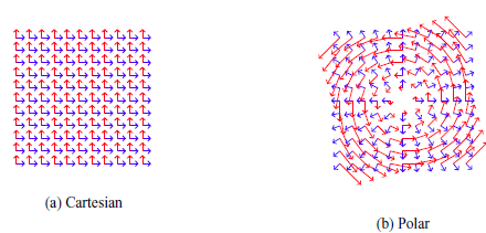
Fig. 5: Possible fields of bases for a local space field covering the Euclidean plane. In both examples, basis vectors are tangent to coordinate lines; either Cartesian or polar coordinates. In the second instance, the basis vectors are undefined at the origin.
5.2 Metrics and index juggling
An important additional structure that one can add to vector spaces are associated metrics. The (covariant) metric, noted g, is what defines the inner product of (local) vectors. It is a tensor field that, when given two vectors as input, returns a scalar, their inner product. One defines the contravariant metric g’ as the inverse of the covariant metric.Footnote
18
This can be specified as $g{_i}{_k}g'{^k}{^j}$
=
$g{_i}{_k}g'{^k}{^j}$
= $\delta_{i}^j$
.
$\delta_{i}^j$
.
To capture this algebraic structure, we distinguish the vector space for which we define the metric as an associated type, $T_{z}$
, of a new category class
$T_{z}$
, of a new category class $\mathsf{MetricCategory}$
.
$\mathsf{MetricCategory}$
.
The various notations for metrics are shown in Figure 6.

Fig. 6: Tensor field primitives in various notations, and their types.
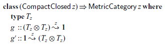
Then we can embed the metric morphism in Albert as follows:
The metric tensor is symmetric—a fact which can be expressed as its antisymmetric part (![]() ) being zero. The coefficients of the matrix representation of the metric are given by the inner product of the basis vectors. For the usual Cartesian basis, the metric is represented by the identity matrix. For the basis
) being zero. The coefficients of the matrix representation of the metric are given by the inner product of the basis vectors. For the usual Cartesian basis, the metric is represented by the identity matrix. For the basis $(\mathbf e_\rho, \mathbf e_\theta)$
defined above, the matrix representation of the metric is
$(\mathbf e_\rho, \mathbf e_\theta)$
defined above, the matrix representation of the metric is
 \begin{equation*}g_\mathsf{Polar} =\left[\begin{array}{cc}\rho^{2}&0\\0&1\end{array}\right]\end{equation*}
With this knowledge, we can define an instance for coordinate representations of the $\mathsf{MetricCategory}$
class:
$\mathsf{MetricCategory}$
class:
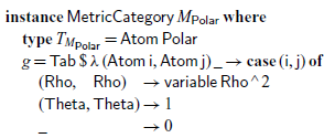
The scalars associated with this additive category are expressions where the variables $\rho$
and
$\rho$
and $\theta$
occur, and the
$\theta$
occur, and the $\mathsf{variable}$
function embeds a coordinate name into such expression types:
$\mathsf{variable}$
function embeds a coordinate name into such expression types:
Thus, the $\mathsf{Polar}$
data type serves triple duty. First, it is the set of variables used in such expressions. Second, it serves to identify the meaning of coordinates as a parameter in the
$\mathsf{Polar}$
data type serves triple duty. First, it is the set of variables used in such expressions. Second, it serves to identify the meaning of coordinates as a parameter in the ![]() type. Third, it is used to construct a representation of the atomic vector space. For the matrix category, an object is a set indexing the base vectors, so
type. Third, it is used to construct a representation of the atomic vector space. For the matrix category, an object is a set indexing the base vectors, so $\mathsf{Atom}$
is a simple wrapper around the coordinate type:
$\mathsf{Atom}$
is a simple wrapper around the coordinate type:
One can contrast the type of metrics with that of $\eta$
and
$\eta$
and $\epsilon$
. First, only the tangent space
$\epsilon$
. First, only the tangent space $T_{z}$
has a metric, while every object has a dual. Indeed,
$T_{z}$
has a metric, while every object has a dual. Indeed, $\eta$
and
$\eta$
and $\epsilon$
are both realised as
$\epsilon$
are both realised as $\delta$
in the tensor instance, and are an identity operation in Einstein notation. They have no geometric significance and thus can be defined generically. In contrast, the metric depends on the geometric properties of the space
$\delta$
in the tensor instance, and are an identity operation in Einstein notation. They have no geometric significance and thus can be defined generically. In contrast, the metric depends on the geometric properties of the space $T_{z}$
that they operate upon. Second, the metrics do not dualise objects, whereas
$T_{z}$
that they operate upon. Second, the metrics do not dualise objects, whereas $\eta$
and
$\eta$
and $\epsilon$
do. Accordingly, our diagrammatic notation does not make any special mark on the input/output wires of metrics. Yet, metrics satisfy a variant of the snake laws:
$\epsilon$
do. Accordingly, our diagrammatic notation does not make any special mark on the input/output wires of metrics. Yet, metrics satisfy a variant of the snake laws: ![]() is equal to
is equal to ![]() .
.
By combining the compact closed categorical structure with metrics, one can construct the following two morphisms (in Roger):

In diagram form $\mathsf{juggleUp}$
is
$\mathsf{juggleUp}$
is ![]() . The existence of such morphisms have a direct consequence on Einstein notation: any subscript index
. The existence of such morphisms have a direct consequence on Einstein notation: any subscript index $\mathsf{P}\mskip 3.0muz\mskip 3.0mu\mathsf{r}\mskip 3.0mu\mathsf{a}$
can be raised into
$\mathsf{P}\mskip 3.0muz\mskip 3.0mu\mathsf{r}\mskip 3.0mu\mathsf{a}$
can be raised into $\mathsf{P}\mskip 3.0muz\mskip 3.0mu\mathsf{r}\mskip 3.0mu{\mathsf{a}^*}$
, and vice versa. In other words, any index can be used as super or subscript as needed. As a first example, given a vector
$\mathsf{P}\mskip 3.0muz\mskip 3.0mu\mathsf{r}\mskip 3.0mu{\mathsf{a}^*}$
, and vice versa. In other words, any index can be used as super or subscript as needed. As a first example, given a vector $v^{i}$
, the covector
$v^{i}$
, the covector $v_i$
is a shorthand for
$v_i$
is a shorthand for $v^kg_{ki}$
. It is important to note that the position of the indices changes the value of the expression: the actual numbers (the components) of a vector
$v^kg_{ki}$
. It is important to note that the position of the indices changes the value of the expression: the actual numbers (the components) of a vector $v^{i}$
are different from those of the corresponding covector
$v^{i}$
are different from those of the corresponding covector $v_i$
unless the metric representation is the identity (as in global Cartesian coordinates). As another example, assuming a tensor
$v_i$
unless the metric representation is the identity (as in global Cartesian coordinates). As another example, assuming a tensor $\mathsf{t}\mskip 3.0mu{:}\mskip 3.0muT_{z}\mskip 3.0mu{\otimes }\mskip 3.0muT_{z}\,\mskip 1.0mu\overset{z}{\leadsto }\mskip 1.0mu\,T_{z}$
, the expression
$\mathsf{t}\mskip 3.0mu{:}\mskip 3.0muT_{z}\mskip 3.0mu{\otimes }\mskip 3.0muT_{z}\,\mskip 1.0mu\overset{z}{\leadsto }\mskip 1.0mu\,T_{z}$
, the expression $t_{ijl}$
is a shorthand for
$t_{ijl}$
is a shorthand for $t_{ij}{}^{k} g_{kl}$
.
$t_{ij}{}^{k} g_{kl}$
.
In the mathematical praxis, raising and lowering indices are also referred to as index juggling. In Albert, index juggling is realised explicitly: our recent example can be written $\mathsf{t}\mskip 3.0mu_{\mathsf{i}}\mskip 3.0mu_{\mathsf{j}}\mskip 3.0mu{(}\mskip 0.0mu\mathsf{raise}\mskip 3.0mu_{\mathsf{l}}\mskip 0.0mu{)}$
. The raising and lowering functions have the following types and are implemented by embedding
$\mathsf{t}\mskip 3.0mu_{\mathsf{i}}\mskip 3.0mu_{\mathsf{j}}\mskip 3.0mu{(}\mskip 0.0mu\mathsf{raise}\mskip 3.0mu_{\mathsf{l}}\mskip 0.0mu{)}$
. The raising and lowering functions have the following types and are implemented by embedding $\mathsf{juggleUp}$
and
$\mathsf{juggleUp}$
and $\mathsf{juggleDown}$
:
$\mathsf{juggleDown}$
:
5.3 Change of global coordinate system
As we have seen, Einstein notation is carefully set up to work without reference to the system of coordinates used to identify positions in the manifold. In practice, this means that one can reason about tensors, their derivatives (Section 5.4), etc. without worrying about the choice of coordinates. It is only at the very last stage that one chooses a system of global coordinates where the data of the problem is easy to express and calculate with. We have seen that one can convert between bases by applying the appropriate transformations on the representation matrices (see Section 2.2). For canonical bases (defined as partial derivatives of the position), the $\mathsf{transform}$
function is obtained by composing with Jacobian. In our running example, we have at our disposal the Jacobian J(T) and its inverse
$\mathsf{transform}$
function is obtained by composing with Jacobian. In our running example, we have at our disposal the Jacobian J(T) and its inverse $J(T^*)$
to convert between polar and Cartesian global coordinates with
$J(T^*)$
to convert between polar and Cartesian global coordinates with $J(T^*) = $ $\left[\begin{array}{cc}\cos{\theta}&\sin{\theta}\\\rho^{-1}\sin{\theta}&-\rho^{-1}\cos{\theta}\end{array}\right]$
.
$\left[\begin{array}{cc}\cos{\theta}&\sin{\theta}\\\rho^{-1}\sin{\theta}&-\rho^{-1}\cos{\theta}\end{array}\right]$
.
As an illustration, let $\tilde v_{\mathsf{Polar}}$
=
$\tilde v_{\mathsf{Polar}}$
= $\left[\begin{array}{cc}-\rho^{-1}&0\end{array}\right]$
be the local coordinates of a co-vector field in the polar tangent basis
$\left[\begin{array}{cc}-\rho^{-1}&0\end{array}\right]$
be the local coordinates of a co-vector field in the polar tangent basis $\tilde v_{\mathsf{Polar}}$ ${:}\mskip 3.0muT_{M_{\mathsf{Polar}}}\mskip 1.0mu\overset{M_{\mathsf{Polar}}}{\leadsto }\mskip 1.0mu\mathbf{1}$
. Then the local coordinates of the co-vector field in the Cartesian tangent basis are given by
${:}\mskip 3.0muT_{M_{\mathsf{Polar}}}\mskip 1.0mu\overset{M_{\mathsf{Polar}}}{\leadsto }\mskip 1.0mu\mathbf{1}$
. Then the local coordinates of the co-vector field in the Cartesian tangent basis are given by ${v_{\mathsf{Cartesian}}}_i = J(T)_i^j {v_{\mathsf{Polar}}}_j$
, and we have:
${v_{\mathsf{Cartesian}}}_i = J(T)_i^j {v_{\mathsf{Polar}}}_j$
, and we have: $\tilde v_{\mathsf{Cartesian}}$
=
$\tilde v_{\mathsf{Cartesian}}$
= $\left[\begin{array}{cc}-\rho^{-1}\cos{\theta}&-\rho^{-1}\sin{\theta}\end{array}\right]$
.
$\left[\begin{array}{cc}-\rho^{-1}\cos{\theta}&-\rho^{-1}\sin{\theta}\end{array}\right]$
.
5.4 Spatial derivative: Levi-Civita connection
The local vector space can change from position to position, but it is assumed to vary smoothly. One says that a connection is defined between neighbouring spaces. This means that we can take the derivative of tensor fields with respect to position. Two cautionary remarks are in order regarding our use of the phrase spatial derivative. First, the terminology is meant to include hyperbolic geometries, thus space-time (Minkowski space) is covered. Second, there are other notions of spatial derivatives, but here we will only consider the case of the Levi-Civita connection, more precisely, which has additional properties: see footnote 20.
Considering the simplest case, the derivative of a scalar field $\mathsf{s}$
is a covector field: its gradient. That is, given a direction vector
$\mathsf{s}$
is a covector field: its gradient. That is, given a direction vector $\vec v$
, the gradient will return the slope of
$\vec v$
, the gradient will return the slope of $\mathsf{s}$
in the
$\mathsf{s}$
in the $\vec v$
direction. In general, the spatial derivative of a tensor takes a vector argument and returns the variation in this direction. So the derivative of a tensor field is itself a tensor field, whose (covariant) order is one more than its argument, and for this reason, the spatial derivative of tensors is called the covariant derivative. We capture this in the following class, which signals the presence of a connection (and spatial derivative) in a category.
$\vec v$
direction. In general, the spatial derivative of a tensor takes a vector argument and returns the variation in this direction. So the derivative of a tensor field is itself a tensor field, whose (covariant) order is one more than its argument, and for this reason, the spatial derivative of tensors is called the covariant derivative. We capture this in the following class, which signals the presence of a connection (and spatial derivative) in a category.
Accordingly, in Einstein notation, the covariant derivative uses an additional (lower) index.
The actual implementation is too involved to present just yet, and deferred to Section 7. In the diagrammatic notation, we represent the covariant derivative as a thick box around the tensor whose derivative is taken. This box adds an input wire for the additional input vector, and propagates the wires of the tensor which it encloses, reflecting the propagation of the types $\mathsf{a}$
and
$\mathsf{a}$
and $\mathsf{b}$
in the type of
$\mathsf{b}$
in the type of $\nabla$
. In Figure 6, we illustrate with a derivative applied to a tensor of order (1,1), but it can be applied to any morphism, with arbitrary domain and codomain—and hence to tensors of arbitrary order. For instance, the covariant derivative of a tensor
$\nabla$
. In Figure 6, we illustrate with a derivative applied to a tensor of order (1,1), but it can be applied to any morphism, with arbitrary domain and codomain—and hence to tensors of arbitrary order. For instance, the covariant derivative of a tensor $\mathsf{t}$
of order (2,2) is written
$\mathsf{t}$
of order (2,2) is written $\nabla{_i}t{_j}{_k}{^l}{^m}$
or
$\nabla{_i}t{_j}{_k}{^l}{^m}$
or  , but (still) ${\nabla}\mskip 3.0mu\mathsf{t}$
in Roger.
${\nabla}\mskip 3.0mu\mathsf{t}$
in Roger.
Example: Laplacian. As a simple example, we express the Laplacian (the divergence of the gradient) of a given scalar field P. Its physical meaning has no bearing on our development; but if P is an energy potential, its gradient is the corresponding force field, and its divergence the density of an associated charge or mass. We write P for the potential field, or ![]() as a diagram. The scalar character of this field is represented by the lack of indices, or the use of the unit object for its domain and codomain. Its gradient is denoted
as a diagram. The scalar character of this field is represented by the lack of indices, or the use of the unit object for its domain and codomain. Its gradient is denoted $\nabla{_i}P$
, or
$\nabla{_i}P$
, or ![]() . Again, indices or objects indicate that we have an order (1,0) (covector) field. At each point, the local covector is a linear function that takes a direction (vector) into the slope in that direction (a scalar).
. Again, indices or objects indicate that we have an order (1,0) (covector) field. At each point, the local covector is a linear function that takes a direction (vector) into the slope in that direction (a scalar).
The Laplacian is a linear combination of second order derivatives. To compute the linear combination, we need to apply contraction, which always expects an upper and a lower index, but we have two covariant (lower) indices, so we must raise one index by multiplying with the contravariant metric. The Einstein notation is $g'{^i}{^j}\nabla{_i}\nabla{_j}P$
, the corresponding diagram is
$g'{^i}{^j}\nabla{_i}\nabla{_j}P$
, the corresponding diagram is ![]() , and in Roger it is
, and in Roger it is ${(}\mskip 0.0mu{\nabla}\mskip 3.0mu{(}\mskip 0.0mu{(}\mskip 0.0mu{\nabla}\mskip 3.0mu\mathsf{P}\mskip 0.0mu{)}\mskip 3.0mu{\circ }\mskip 3.0mu\rho\mskip 0.0mu{)}\mskip 0.0mu{)}\mskip 3.0mu{\circ }\mskip 3.0mu\mathsf{g'}$
. The Einstein notation, while already economical, can be made even more concise by using the index juggling convention:
${(}\mskip 0.0mu{\nabla}\mskip 3.0mu{(}\mskip 0.0mu{(}\mskip 0.0mu{\nabla}\mskip 3.0mu\mathsf{P}\mskip 0.0mu{)}\mskip 3.0mu{\circ }\mskip 3.0mu\rho\mskip 0.0mu{)}\mskip 0.0mu{)}\mskip 3.0mu{\circ }\mskip 3.0mu\mathsf{g'}$
. The Einstein notation, while already economical, can be made even more concise by using the index juggling convention: $\nabla_{i}\nabla^i P$
. In Albert, the same thing would be written
$\nabla_{i}\nabla^i P$
. In Albert, the same thing would be written
Here the high index from the contraction must be lowered because $\mathsf{deriv}$
can only take a low index as its first argument.
$\mathsf{deriv}$
can only take a low index as its first argument.
5.4.1 Laws of covariant derivatives
As one might expect, the covariant derivative satisfies the product law for derivatives:
 \begin{equation}\nabla_{i} (t u) = (\nabla_{i} t) u + t (\nabla_{i} u)\end{equation}
The above formulation is concise, but using it as basis for implementation can be tedious, because one needs to track free and bound variables. A pitfall is that t and u stand for arbitrary expressions, and index variables may occur free in them. Therefore, a specific implementation difficulty is that one needs to preserve the linearity of index variables at the level of the host language.Footnote
19
Thus, we find that the morphism edsl Roger is a better implementation vehicle in this case. The laws become noticeably more verbose, but not horribly so, and dispense of tracking free variables. In this notation, the product law is expressed as two cases, one for each of the composition ${(}\mskip 0.0mu{\circ }\mskip 0.0mu{)}$
and tensor
${(}\mskip 0.0mu{\circ }\mskip 0.0mu{)}$
and tensor ${(}\mskip 0.0mu{\otimes }\mskip 0.0mu{)}$
operators:
${(}\mskip 0.0mu{\otimes }\mskip 0.0mu{)}$
operators:
 \begin{align*}{\nabla}\mskip 3.0mu{(}\mskip 0.0mu\mathsf{t}\mskip 3.0mu{\circ }\mskip 3.0mu\mathsf{u}\mskip 0.0mu{)}&=\mathsf{t}\mskip 3.0mu{\circ }\mskip 3.0mu{(}\mskip 0.0mu{\nabla}\mskip 3.0mu\mathsf{u}\mskip 0.0mu{)}\mskip 3.0mu{+}\mskip 3.0mu{(}\mskip 0.0mu{\nabla}\mskip 3.0mu\mathsf{t}\mskip 0.0mu{)}\mskip 3.0mu{\circ }\mskip 3.0mu{(}\mskip 0.0mu\mathsf{id}\mskip 3.0mu{\otimes }\mskip 3.0mu\mathsf{u}\mskip 0.0mu{)}\\{\nabla}\mskip 3.0mu{(}\mskip 0.0mu\mathsf{t}\mskip 3.0mu{\otimes }\mskip 3.0mu\mathsf{u}\mskip 0.0mu{)}&={(}\mskip 0.0mu{\nabla}\mskip 3.0mu\mathsf{t}\mskip 3.0mu{\otimes }\mskip 3.0mu\mathsf{u}\mskip 0.0mu{)}\mskip 3.0mu{\circ }\mskip 3.0mu\bar{\alpha}\mskip 3.0mu{+}\mskip 3.0mu{(}\mskip 0.0mu\mathsf{t}\mskip 3.0mu{\otimes }\mskip 3.0mu{\nabla}\mskip 3.0mu\mathsf{u}\mskip 0.0mu{)}\mskip 3.0mu{\circ }\mskip 3.0mu\alpha\mskip 3.0mu{\circ }\mskip 3.0mu{(}\mskip 0.0mu\sigma \mskip 3.0mu{\otimes }\mskip 3.0mu\mathsf{id}\mskip 0.0mu{)}\mskip 3.0mu{\circ }\mskip 3.0mu\bar{\alpha}\end{align*}
As before, we find the corresponding diagrams more readable:

The derivative of all constant morphisms is zero: $\nabla\mskip 3.0mu\mathsf{id}\mskip 3.0mu{=}\mskip 3.0mu\mathrm{0}$
,
$\nabla\mskip 3.0mu\mathsf{id}\mskip 3.0mu{=}\mskip 3.0mu\mathrm{0}$
, $\nabla\mskip 3.0mu\rho\mskip 3.0mu{=}\mskip 3.0mu\mathrm{0}$
,
$\nabla\mskip 3.0mu\rho\mskip 3.0mu{=}\mskip 3.0mu\mathrm{0}$
, $\nabla\mskip 3.0mu\alpha\mskip 3.0mu{=}\mskip 3.0mu\mathrm{0}$
, etc. This property also holds for the (co)metric tensors:Footnote 20
$\nabla\mskip 3.0mu\alpha\mskip 3.0mu{=}\mskip 3.0mu\mathrm{0}$
, etc. This property also holds for the (co)metric tensors:Footnote 20 $\nabla\mskip 3.0mug\mskip 3.0mu{=}\mskip 3.0mu\mathrm{0}\mskip 3.0mu{=}\mskip 3.0mu\nabla\mskip 3.0mug'$
. Together, the above laws fully specify the structural behaviour of the derivative and the implementation of the covariant derivative falls out from them with no additional difficulty. However, the important case of the derivative of a tensor in a coordinate category remains to be addressed. This question leads us to the concept of affinity.
$\nabla\mskip 3.0mug\mskip 3.0mu{=}\mskip 3.0mu\mathrm{0}\mskip 3.0mu{=}\mskip 3.0mu\nabla\mskip 3.0mug'$
. Together, the above laws fully specify the structural behaviour of the derivative and the implementation of the covariant derivative falls out from them with no additional difficulty. However, the important case of the derivative of a tensor in a coordinate category remains to be addressed. This question leads us to the concept of affinity.
5.4.2 Partial derivatives, christoffel symbols and affinities
One may be tempted to think that the coefficient representation of the covariant derivative is the index-wise derivative of the coefficient representations. While this is true if the metric is the identity everywhere on the manifold, it is not the case in general.
Conventionally, one speaks of the “partial derivative” for the index-wise derivative of coefficients and retains the term “covariant derivative” for the spatial derivative. (The notations are shown in Figure 6, but note that $\partial_{i}t$
stands for the partial derivative of the expression
$\partial_{i}t$
stands for the partial derivative of the expression $\mathsf{t}$
with respect to the
$\mathsf{t}$
with respect to the $i\text{th}$
coordinate, sometimes also written
$i\text{th}$
coordinate, sometimes also written $\partial t/\partial x^i $
.) As usual, we express the availability of this new operation by means of a class:
$\partial t/\partial x^i $
.) As usual, we express the availability of this new operation by means of a class:
The Levi-Civita connection is unique for a given metric, but we still require the user to provide an implementation. For categories with coordinates, discussed in the next subsection, a canonical implementation of $\nabla$
is provided.
$\nabla$
is provided.
We make the concept available in Albert like this:
In the general case, to compute the covariant derivative, one must account for the variation of the basis. Therefore, the partial derivative must be corrected by a so called affinity term. The partial derivative accounts for the variation of (the representation of) the tensor field itself as the position varies, while the affinity term accounts for the variation of the basis. The variation of the basis is measured by the Christoffel symbol, denoted $\Gamma$
and of type
$\Gamma$
and of type ${(}\mskip 0.0muT_{z}\mskip 3.0mu{\otimes }\mskip 3.0muT_{z}\mskip 0.0mu{)}\,\mskip 1.0mu\overset{z}{\leadsto }\mskip 1.0mu\,T_{z}$
(Figure 6). Different choices of local basis field for the same manifold will yield different values for it. (Therefore, even though
${(}\mskip 0.0muT_{z}\mskip 3.0mu{\otimes }\mskip 3.0muT_{z}\mskip 0.0mu{)}\,\mskip 1.0mu\overset{z}{\leadsto }\mskip 1.0mu\,T_{z}$
(Figure 6). Different choices of local basis field for the same manifold will yield different values for it. (Therefore, even though $\Gamma$
is a morphism in a matrix category, and even though it can be transformed to another basis by multiplication with Jacobians, this transformed version will not be the Christoffel symbol for the new basis. This fact is sometimes expressed in textbooks as “
$\Gamma$
is a morphism in a matrix category, and even though it can be transformed to another basis by multiplication with Jacobians, this transformed version will not be the Christoffel symbol for the new basis. This fact is sometimes expressed in textbooks as “ $\Gamma$
is not a tensor.”)
$\Gamma$
is not a tensor.”)
The Christoffel symbol is often treated abstractly, but it is determined by the (coefficient representation of) the metric:
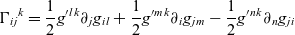 \begin{equation}\Gamma{_i}{_j}{^k} = \frac{1}{2}g'{^l}{^k}\partial{_j}g{_i}{_l} + \frac{1}{2}g'{^m}{^k}\partial{_i}g{_j}{_m} - \frac{1}{2}g'{^n}{^k}\partial{_n}g{_j}{_i}\end{equation}
The Christoffel symbol is always symmetric in its first two indices, which is equivalent to asserting that the following diagram is zero: ![]() . In the implementation, we make
. In the implementation, we make $\Gamma$
a method of the class
$\Gamma$
a method of the class $\mathsf{CoordinateCategory}$
, but with a default definition in terms of Equation (5.4). We make it available in Albert by embedding the morphism
$\mathsf{CoordinateCategory}$
, but with a default definition in terms of Equation (5.4). We make it available in Albert by embedding the morphism $\Gamma$
as follows:
$\Gamma$
as follows:
For 2-dimensional atomic vector space, the Christoffel symbol has $2^3=8$
components. For our running example of the polar coordinate system and associated canonical tangent space, we can write
$2^3=8$
components. For our running example of the polar coordinate system and associated canonical tangent space, we can write $\Gamma$
as two
$\Gamma$
as two $2 \times 2$
symmetric matrices, as follows:
$2 \times 2$
symmetric matrices, as follows:
 \begin{align*}\Gamma^{\rho} =\left[\begin{array}{cc}0&0\\0&-\rho\end{array}\right] \quad\Gamma^{\theta} =\left[\begin{array}{cc}0&1/\rho\\1/\rho&0\end{array}\right]\end{align*}
In textbooks on tensors, for instance that of Lovelock & Rund (Reference Lovelock and Rund1989), one often sees the relation between covariant and partial derivatives expressed as a family of equations, depending on the order of the tensor whose derivative is taken:
 \begin{align*}\nabla_{i} T& = \partial_{i} T\\\nabla_{i} T_j& = \partial_{i} T_j - \Gamma_{ij}{^k} T_k \\\nabla_{i} T^j& = \partial_{i} T^j + \Gamma_{ik}{^j} T^k\\\nabla_{i} T_j{^k}& = \partial_{i} T_j{^k} - \Gamma_{il}{^k} T_j{^l} + \Gamma_{ij}{^l} T_l {^k}\end{align*}
etc. Using this sort of definition is particularly error prone (can you spot quickly whether there is a mistake in the last line?). In contrast, Roger captures all cases in one go:
The complexity is pushed down into $\mathsf{affinity}$
, which is invoked once for the domain and once for the codomain of
$\mathsf{affinity}$
, which is invoked once for the domain and once for the codomain of $\mathsf{t}$
. The affinity is a family of morphisms
$\mathsf{t}$
. The affinity is a family of morphisms $\mathsf{affinity}\mskip 3.0mu{::}\mskip 3.0muT_{M_{\mathsf{b}}}\mskip 3.0mu{\otimes }\mskip 3.0mu\mathsf{a}\,\mskip 1.0mu\overset{M_{\mathsf{b}}}{\leadsto }\mskip 1.0mu\,\mathsf{a}$
for any object
$\mathsf{affinity}\mskip 3.0mu{::}\mskip 3.0muT_{M_{\mathsf{b}}}\mskip 3.0mu{\otimes }\mskip 3.0mu\mathsf{a}\,\mskip 1.0mu\overset{M_{\mathsf{b}}}{\leadsto }\mskip 1.0mu\,\mathsf{a}$
for any object $\mathsf{a}$
constructed from the local vector space
$\mathsf{a}$
constructed from the local vector space $T_{M_{\mathsf{b}}}$
and refers to a specific basis for it, using some coherent canonical choice of bases (with
$T_{M_{\mathsf{b}}}$
and refers to a specific basis for it, using some coherent canonical choice of bases (with $\mathsf{b}$
as a basis for
$\mathsf{b}$
as a basis for $T_{M_{\mathsf{b}}}$
). The affinity for arbitrary vector spaces is defined by induction on the structure of the corresponding object. The affinity for a product object is the sum of affinities for each of the components, leaving the other component untouched. The affinity for a dual object is the negative affinity of the underlying object, with input and output suitably swapped. This can be coded by a type-dependent set of equations:Footnote 21
$T_{M_{\mathsf{b}}}$
). The affinity for arbitrary vector spaces is defined by induction on the structure of the corresponding object. The affinity for a product object is the sum of affinities for each of the components, leaving the other component untouched. The affinity for a dual object is the negative affinity of the underlying object, with input and output suitably swapped. This can be coded by a type-dependent set of equations:Footnote 21

Here, Albert is much more concise than Roger (we omit the corresponding expressions entirely). The corresponding graphical notation is shown in Figure 7 for each case (but using atomic types in place of a proper induction).

Fig. 7: Affinities $\mathsf{aff}\mskip 3.0mu\mathsf{a}$
at various types
$\mathsf{aff}\mskip 3.0mu\mathsf{a}$
at various types $\mathsf{a}$
(shown in the third row).
$\mathsf{a}$
(shown in the third row).
5.5 Example: Computing the Laplacian in an arbitrary coordinate system
Returning to the example of the potential field, Equation (5.5) and $\mathsf{aff}$
tell us that its covariant derivative is equal to its partial derivative, regardless of the value of
$\mathsf{aff}$
tell us that its covariant derivative is equal to its partial derivative, regardless of the value of $\Gamma$
:
$\Gamma$
: $\nabla{_i}P$
=
$\nabla{_i}P$
= $\partial{_i}P$
. Indeed, its domain and codomain are both
$\partial{_i}P$
. Indeed, its domain and codomain are both $\mathbf{1}$
, and therefore the affinities are both zero. (To compute the value of
$\mathbf{1}$
, and therefore the affinities are both zero. (To compute the value of $\nabla{_i}P$
in a given coordinate system, one would still need to multiply by the Jacobian as indicated earlier.)
$\nabla{_i}P$
in a given coordinate system, one would still need to multiply by the Jacobian as indicated earlier.)
However, when computing the second derivative, a non-zero affinity arises (because the 1st derivative has a non-unit domain.) One has therefore:
 \begin{equation}\nabla_{i}\nabla^i P =g'{^i}{^j}\nabla{_i}\nabla{_j}P=g'{^i}{^j}\partial{_i}\partial{_j}P - g'{^k}{^l}\Gamma{_k}{_l}{^m}\partial{_m}P\end{equation}
In diagram notation: 
As an illustration, let us compute the Laplacian of the scalar field defined as growing with the negated logarithm of the distance to the origin: $P = -\log(\rho)$
.
$P = -\log(\rho)$
.
Its covariant derivative (or gradient) is given by the partial derivatives in polar coordinates (because $\mathsf{aff}\mskip 3.0mu\mathbf{1}\mskip 3.0mu{=}\mskip 3.0mu\mathrm{0}$
, as already mentioned). The components in the polar tangent basis are
$\mathsf{aff}\mskip 3.0mu\mathbf{1}\mskip 3.0mu{=}\mskip 3.0mu\mathrm{0}$
, as already mentioned). The components in the polar tangent basis are
 \begin{equation*}\nabla P = \partial P - 0 + 0 = \left[\begin{array}{cc}\partial P/\partial\rho&\partial P/\partial\theta\end{array}\right]=\left[\begin{array}{cc}-\rho^{-1}&0\end{array}\right]\end{equation*}
We have seen above that, by composing with the appropriate Jacobian, the components of the gradient in the Cartesian tangent basis are $\left[\begin{array}{cc}-\rho^{-1}\cos{\theta}&-\rho^{-1}\sin{\theta}\end{array}\right]$
.
$\left[\begin{array}{cc}-\rho^{-1}\cos{\theta}&-\rho^{-1}\sin{\theta}\end{array}\right]$
.
The second derivative ( $\nabla\nabla P$
) is a second-order tensor, and computing it manually in the Cartesian basis is error-prone. In contrast, because P has radial symmetry, in the polar tangent basis its partial derivative
$\nabla\nabla P$
) is a second-order tensor, and computing it manually in the Cartesian basis is error-prone. In contrast, because P has radial symmetry, in the polar tangent basis its partial derivative $\partial P$
has a simple expression (the co-vector
$\partial P$
has a simple expression (the co-vector $\left[\begin{array}{cc}-\rho^{-1}&0\end{array}\right]$
). Thus, only the
$\left[\begin{array}{cc}-\rho^{-1}&0\end{array}\right]$
). Thus, only the $\rho-\rho$
-component of the second partial derivative is non-zero:
$\rho-\rho$
-component of the second partial derivative is non-zero: $\partial^2P/\partial\rho^2 = \rho^{-2}$
. To compute the covariant derivative, we also need the affinity term, which is obtained by multiplying the gradient
$\partial^2P/\partial\rho^2 = \rho^{-2}$
. To compute the covariant derivative, we also need the affinity term, which is obtained by multiplying the gradient $\nabla P$
by
$\nabla P$
by $\Gamma$
, then multiply by the contravariant metric (recall Equation 5.6). Because only the
$\Gamma$
, then multiply by the contravariant metric (recall Equation 5.6). Because only the $\mathbf e_\rho$
coefficient of
$\mathbf e_\rho$
coefficient of $\nabla P$
is non-zero, is suffices to multiply this component (
$\nabla P$
is non-zero, is suffices to multiply this component ( $-\rho^{-1}$
) by
$-\rho^{-1}$
) by $\Gamma^\rho$
to obtain the affinity term
$\Gamma^\rho$
to obtain the affinity term $\left[\begin{array}{cc}0&0\\0&1\end{array}\right]$
. Finally, we get
$\left[\begin{array}{cc}0&0\\0&1\end{array}\right]$
. Finally, we get $\nabla\nabla P$
(in polar tangent coordinates) from Equation (5.5): the partial derivative minus the affinity we computed above plus the second affinity which is zero (because the output space is
$\nabla\nabla P$
(in polar tangent coordinates) from Equation (5.5): the partial derivative minus the affinity we computed above plus the second affinity which is zero (because the output space is $\mathbf{1}$
) which gives us
$\mathbf{1}$
) which gives us $\left[\begin{array}{cc}\rho^{-2}&0\\0&-1\end{array}\right]$
.
$\left[\begin{array}{cc}\rho^{-2}&0\\0&-1\end{array}\right]$
.
The Laplacian is obtained by 2-way contraction with the contravariant metric. One way to do this is to multiply the above by the contravariant metric, to get $\left[\begin{array}{cc}\rho^{-2}&0\\0&-\rho^{-2}\end{array}\right]$
, and take the trace, which is zero for
$\left[\begin{array}{cc}\rho^{-2}&0\\0&-\rho^{-2}\end{array}\right]$
, and take the trace, which is zero for $\rho>0$
. (Note that even if it were non-zero there was no need to multiply by any Jacobian because the divergence field is scalar.) The fact that the Laplacian of this scalar field is zero means that the charge density is zero away from the origin: in a two-dimensional space the potential of a point charge at the origin is proportional to this scalar field P.
$\rho>0$
. (Note that even if it were non-zero there was no need to multiply by any Jacobian because the divergence field is scalar.) The fact that the Laplacian of this scalar field is zero means that the charge density is zero away from the origin: in a two-dimensional space the potential of a point charge at the origin is proportional to this scalar field P.
Beyond its illustrative benefits, a takeaway from this example is that all computations were free of trigonometry, and involved many zeros, thanks to the choice of a global coordinate system which had a zero gradient in one of the axes. Even though each step in the computations was presented for illustrative purposes, the $\mathsf{MetricCategory}\mskip 3.0muM_{\mathsf{Polar}}$
instance meant that we could run all the above computations as Haskell programs.
$\mathsf{MetricCategory}\mskip 3.0muM_{\mathsf{Polar}}$
instance meant that we could run all the above computations as Haskell programs.
5.6 Tensor calculus summary
Athis point we have presented all the classes whose morphisms constitute the combinators of Roger. Their relationships are summarised in Figure 8.
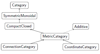
Fig. 8: Inheritance relationships between tensor structures. In the praxis, every instance of a category with a metric $\mathsf{Additive}$
is also additive. However, diagrams don’t support a good representation for addition, so the dotted line is implemented as a subclass relationship in our library.
$\mathsf{Additive}$
is also additive. However, diagrams don’t support a good representation for addition, so the dotted line is implemented as a subclass relationship in our library.
When it comes to Albert, we have two separate sub-languages. First, we have a number of combinators which only manipulate indices, shown in Figure 9. Indices can be split, merged, raised and lowered. Indices for unit vector-spaces are unimportant and can be created or discarded at will. Second, we have a number of combinators which nominally manipulate scalar-valued expressions (addition, multiplication, embedding of constant tensors, Kronecker delta, and contraction, etc; see Figure 10). Various combinators require various amounts of structure in the underlying category z.
The semantics in terms of morphisms is provided by the $\mathsf{tensorEval}$
function, and
$\mathsf{tensorEval}$
function, and $\mathsf{tensorEval}_{1}$
for the special case of closed tensor expressions. For tensor fields, primitives for metrics and derivatives are also available.
$\mathsf{tensorEval}_{1}$
for the special case of closed tensor expressions. For tensor fields, primitives for metrics and derivatives are also available.
6 Application: Curvature and general relativity
To further demonstrate the applicability of Albert, in this section, we present some concepts of general relativity, with particular focus on the notion of curvature. General relativity can be summarised as “matter curves space-time”. This informal statement can be expressed as a tensor equation as follows:
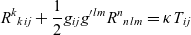 \begin{equation}R{^k}{_k}{_i}{_j} + \frac{1}{2}g{_i}{_j}g'{^l}{^m}R{^n}{_n}{_l}{_m} = \kappa T{_i}{_j}\end{equation}
In the above, $T{_i}{_j}$
represents the contents of space-time in terms of energy, momentum, pressure, etc. depending on the components of the tensor. The gravitational constant is
$T{_i}{_j}$
represents the contents of space-time in terms of energy, momentum, pressure, etc. depending on the components of the tensor. The gravitational constant is $\kappa$
.Footnote
22
The tensor
$\kappa$
.Footnote
22
The tensor $R{^l}{_i}{_j}{_k}$
captures the curvature properties of space-time, and its value solely depends on the metric, as we will see below. Thus, solving the equation for a given
$R{^l}{_i}{_j}{_k}$
captures the curvature properties of space-time, and its value solely depends on the metric, as we will see below. Thus, solving the equation for a given $T{_i}{_j}$
amounts to finding a suitable metric. Given such a solution, we can compute the expression for the left-hand-side of the equation and verify that it is equal to the right-hand side. We do so for the example of a point mass in Section 6.2. Before that, we discuss in more detail
$T{_i}{_j}$
amounts to finding a suitable metric. Given such a solution, we can compute the expression for the left-hand-side of the equation and verify that it is equal to the right-hand side. We do so for the example of a point mass in Section 6.2. Before that, we discuss in more detail $R{^l}{_i}{_j}{_k}$
, the Riemann curvature tensor.
$R{^l}{_i}{_j}{_k}$
, the Riemann curvature tensor.
Definition 6 (Riemann curvature). The Riemann curvature is a 4-tensor, given by the following identity: $R{^l}{_i}{_j}{_k}$
=
$R{^l}{_i}{_j}{_k}$
= $\partial{_i}\Gamma{_j}{_k}{^l} - \partial{_j}\Gamma{_i}{_k}{^l} + \Gamma{_i}{_m}{^l}\Gamma{_j}{_k}{^m} - \Gamma{_j}{_n}{^l}\Gamma{_i}{_k}{^n}$
.
$\partial{_i}\Gamma{_j}{_k}{^l} - \partial{_j}\Gamma{_i}{_k}{^l} + \Gamma{_i}{_m}{^l}\Gamma{_j}{_k}{^m} - \Gamma{_j}{_n}{^l}\Gamma{_i}{_k}{^n}$
.
Each pair of terms is the antisymmetric part of a 4-tensor. Taking advantage of this property, we can make the diagram notation a sum of two terms: ![]() . In Roger, it is even possible to factor the antisymmetrisation operator and obtain the following concise expression:
. In Roger, it is even possible to factor the antisymmetrisation operator and obtain the following concise expression: ${(}\mskip 0.0mu{\partial}\mskip 3.0mu\Gamma\mskip 3.0mu{+}\mskip 3.0mu\Gamma\mskip 3.0mu{\circ }\mskip 3.0mu{(}\mskip 0.0mu\mathsf{id}\mskip 3.0mu{\otimes }\mskip 3.0mu\Gamma\mskip 0.0mu{)}\mskip 0.0mu{)}\mskip 3.0mu{\circ }\mskip 3.0mu\alpha\mskip 3.0mu{\circ }\mskip 3.0mu{(}\mskip 0.0mu{(}\mskip 0.0mu\mathsf{id}\mskip 3.0mu{-}\mskip 3.0mu\sigma \mskip 0.0mu{)}\mskip 3.0mu{\otimes }\mskip 3.0mu\mathsf{id}\mskip 0.0mu{)}$
. Despite its concision, this form obscures which index plays which role, and thus is rarely found in the literature. The above definition can be encoded directly in Albert as follows:
${(}\mskip 0.0mu{\partial}\mskip 3.0mu\Gamma\mskip 3.0mu{+}\mskip 3.0mu\Gamma\mskip 3.0mu{\circ }\mskip 3.0mu{(}\mskip 0.0mu\mathsf{id}\mskip 3.0mu{\otimes }\mskip 3.0mu\Gamma\mskip 0.0mu{)}\mskip 0.0mu{)}\mskip 3.0mu{\circ }\mskip 3.0mu\alpha\mskip 3.0mu{\circ }\mskip 3.0mu{(}\mskip 0.0mu{(}\mskip 0.0mu\mathsf{id}\mskip 3.0mu{-}\mskip 3.0mu\sigma \mskip 0.0mu{)}\mskip 3.0mu{\otimes }\mskip 3.0mu\mathsf{id}\mskip 0.0mu{)}$
. Despite its concision, this form obscures which index plays which role, and thus is rarely found in the literature. The above definition can be encoded directly in Albert as follows:
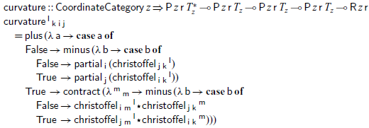
Unfortunately, the operands of each addition must be written in the branch of a case expression, making the expression verbose as a whole. Even though it is defined in terms of Christoffel symbols, the Riemann curvature (as an algebraic object) does not depend on the choice of coordinates. This is a consequence of Theorem 1.
Theorem 1 (Ricci identity). For every covector field $\mathsf{u}$
,
$\mathsf{u}$
, $\nabla{_i}\nabla{_j}u{^k} - \nabla{_j}\nabla{_i}u{^k}$
=
$\nabla{_i}\nabla{_j}u{^k} - \nabla{_j}\nabla{_i}u{^k}$
= $R{^k}{_i}{_j}{_l}u{^l}$
Proof We carry out the proof using the diagram notation. To be sure, we don’t claim that the diagrammatic proof is novel, it is a mere illustration. But we feel it is a good example of using the dsls: all the steps are defined, type checked, and diagrams are rendered with our library. We note first the following lemma: ![]() which is an instance of Equation (5.5).
which is an instance of Equation (5.5).
We then compute symbolically the left-hand-side in the theorem’s statement, starting with the expansion of the outer derivative into partial derivatives and affinity terms (Equation 5.5):
The middle term is zero, by symmetry of $\Gamma$
. Expanding the first term using the lemma and linearity of partial derivatives, we get
$\Gamma$
. Expanding the first term using the lemma and linearity of partial derivatives, we get
Because partial derivatives commute, the first term is zero. We expand the middle term using the composition rule (Equation 5.2) for partial derivatives:

then use the product law, Equation (5.3), on the middle term, and obtain
The partial derivative of the identity morphism is zero so the whole second term can be simplified away
then we commute swap and antisymmetrisation, so the middle term changes sign:
then we use the lemma again to expand $\nabla u$
in the last term
$\nabla u$
in the last term
and note that the middle two terms cancel to yield:
To get to the intended result, it remains to use the structural laws of smcs.
6.1 Code for Equation (6.1)
A contraction of the Riemann curvature occurs twice in Equation (6.1), and as such deserves to be extracted as an intermediate definition. It is called the Ricci tensor.
This tensor can be contracted one more time to obtain what is called the scalar (or Gaussian) curvature:
From there, the left-hand-side of Equation (6.1) is defined as follows:
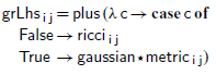
We can then convert it to a morphism:

In the above, the operator & is the linear post-fix application:
6.2 Point-mass example (the Schwarzschild metric)
To complete our test case for Albert, in this section, we define the metric which describes the gravitational effects of a point-sized mass: the Schwarzschild metric. We then verify that this metric satisfies of Equation (6.1) by evaluating both sides and checking that they match.
The first step is to define the coordinate system. Roughly speaking, Schwarzschild coordinates are spherical coordinates with an extra component for time.
The point mass will be located at the origin ( $\rho=0$
) at every point in time. In other words, the mass is at rest in this coordinate system. Hence, because we have a point-mass, the
$\rho=0$
) at every point in time. In other words, the mass is at rest in this coordinate system. Hence, because we have a point-mass, the $T{_i}{_j}$
tensor is zero everywhere except at the origin, where it is infinite.
$T{_i}{_j}$
tensor is zero everywhere except at the origin, where it is infinite.
As for all coordinate representations, the compact-closed category structure for $\mathsf{Matrix}\mskip 3.0mu\mathsf{Spherical}$
falls out directly from Section 3.1. Likewise for the partial derivative. The only missing piece of the structure is the metric. The Schwarzschild metric is defined in terms of the considered mass M or alternatively by the Schwarzschild radius
$\mathsf{Matrix}\mskip 3.0mu\mathsf{Spherical}$
falls out directly from Section 3.1. Likewise for the partial derivative. The only missing piece of the structure is the metric. The Schwarzschild metric is defined in terms of the considered mass M or alternatively by the Schwarzschild radius $r_s$
, the two being connected by the equation
$r_s$
, the two being connected by the equation $r_s = \kappa Mc^2/4\pi$
. We use the parameter
$r_s = \kappa Mc^2/4\pi$
. We use the parameter $r_s$
in the rest of the section. The metric is then given by tabulating the following function as a matrix.
$r_s$
in the rest of the section. The metric is then given by tabulating the following function as a matrix.
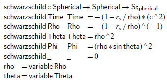
We refer the reader to a course in general relativity for the physical meaning of it. We can then define the $\mathsf{Matrix}\mskip 3.0mu\mathsf{Spherical}$
instance as follows:
$\mathsf{Matrix}\mskip 3.0mu\mathsf{Spherical}$
instance as follows:

At this point, we can directly evaluate $\mathsf{grLhsM}$
with
$\mathsf{grLhsM}$
with $z\mskip 3.0mu{=}\mskip 3.0mu\mathsf{Matrix}\mskip 3.0mu\mathsf{Spherical}$
, and obtain a 4 by 4 matrix of symbolic expressions depending on
$z\mskip 3.0mu{=}\mskip 3.0mu\mathsf{Matrix}\mskip 3.0mu\mathsf{Spherical}$
, and obtain a 4 by 4 matrix of symbolic expressions depending on $\mathsf{Spherical}$
coordinate variables. We find that it simplifies to zero everywhere it is defined.Footnote 23 Thus, we can verify that the Schwarzschild metric satisfies the general relativity equation.
$\mathsf{Spherical}$
coordinate variables. We find that it simplifies to zero everywhere it is defined.Footnote 23 Thus, we can verify that the Schwarzschild metric satisfies the general relativity equation.
7 Implementation of
${\mathbf{A}\scriptstyle \mathbf{LBERT}}$

In this section, we explain the implementation of the combinators of Albert (Figures 9 and 10). As outlined in Section 1.1 and in first approximation, it is provided by the library for symmetric monoidal categories of Bernardy & Spiwack (Reference Bernardy and Spiwack2021). The key idea is that every linear function $\forall\mskip 3.0mu\mathsf{r}\mskip 1.0mu.\mskip 3.0mu\mathsf{P}\mskip 3.0muz\mskip 3.0mu\mathsf{r}\mskip 3.0mu\mathsf{a}\mskip 3.0mu{\multimap }\mskip 3.0mu\mathsf{P}\mskip 3.0muz\mskip 3.0mu\mathsf{r}\mskip 3.0mu\mathsf{b}$
can be converted (naturally) to a morphism of type
$\forall\mskip 3.0mu\mathsf{r}\mskip 1.0mu.\mskip 3.0mu\mathsf{P}\mskip 3.0muz\mskip 3.0mu\mathsf{r}\mskip 3.0mu\mathsf{a}\mskip 3.0mu{\multimap }\mskip 3.0mu\mathsf{P}\mskip 3.0muz\mskip 3.0mu\mathsf{r}\mskip 3.0mu\mathsf{b}$
can be converted (naturally) to a morphism of type $\mathsf{a}\,\mskip 1.0mu\overset{z}{\leadsto }\mskip 1.0mu\,\mathsf{b}$
, and back:
$\mathsf{a}\,\mskip 1.0mu\overset{z}{\leadsto }\mskip 1.0mu\,\mathsf{b}$
, and back:
In fact, any smc z is isomorphic to the category of Haskell linear functions between corresponding ports (whose hom-set family is $\mathsf{Hom}\mskip 3.0mu{(}\mskip 0.0mu\mathsf{a}\mskip 0.0mu{,}\mskip 3.0mu\mathsf{b}\mskip 0.0mu{)}\mskip 3.0mu{=}\mskip 3.0mu{\forall}\mskip 3.0mu\mathsf{r}\mskip 1.0mu.\mskip 3.0mu\mathsf{P}\mskip 3.0muz\mskip 3.0mu\mathsf{r}\mskip 3.0mu\mathsf{a}\mskip 3.0mu{\multimap }\mskip 3.0mu\mathsf{P}\mskip 3.0muz\mskip 3.0mu\mathsf{r}\mskip 3.0mu\mathsf{b}$
). This works even if z has additional structure, and in particular if it is a tensor category.
$\mathsf{Hom}\mskip 3.0mu{(}\mskip 0.0mu\mathsf{a}\mskip 0.0mu{,}\mskip 3.0mu\mathsf{b}\mskip 0.0mu{)}\mskip 3.0mu{=}\mskip 3.0mu{\forall}\mskip 3.0mu\mathsf{r}\mskip 1.0mu.\mskip 3.0mu\mathsf{P}\mskip 3.0muz\mskip 3.0mu\mathsf{r}\mskip 3.0mu\mathsf{a}\mskip 3.0mu{\multimap }\mskip 3.0mu\mathsf{P}\mskip 3.0muz\mskip 3.0mu\mathsf{r}\mskip 3.0mu\mathsf{b}$
). This works even if z has additional structure, and in particular if it is a tensor category.
So, if we were to choose $\mathsf{R}\mskip 3.0muz\mskip 3.0mu\mathsf{r}$
to be
$\mathsf{R}\mskip 3.0muz\mskip 3.0mu\mathsf{r}$
to be $\mathsf{P}\mskip 3.0muz\mskip 3.0mu\mathsf{r}\mskip 3.0mu\mathbf{1}$
, the
$\mathsf{P}\mskip 3.0muz\mskip 3.0mu\mathsf{r}\mskip 3.0mu\mathbf{1}$
, the $\mathsf{encode}$
and
$\mathsf{encode}$
and $\mathsf{decode}$
functions would take care of most of the respective tasks of
$\mathsf{decode}$
functions would take care of most of the respective tasks of $\mathsf{tensorEmbed}$
and
$\mathsf{tensorEmbed}$
and $\mathsf{tensorEval}$
. It would remain to dualise the codomain and apply unitors appropriately, as shown in Figure 4(a).
$\mathsf{tensorEval}$
. It would remain to dualise the codomain and apply unitors appropriately, as shown in Figure 4(a).
With this simple setup, we can implement the embedding of tensors (including $\delta$
), as well as multiplication. Unfortunately, there are several complications.
$\delta$
), as well as multiplication. Unfortunately, there are several complications.
7.1 Complication: Supporting derivatives
The main issue with the above implementation sketch arises when trying to implement the covariant derivative of a tensor expression $\mathsf{t}$
as a sum of its partial derivative and affinity terms. Indeed, the affinity terms of a tensor expression
$\mathsf{t}$
as a sum of its partial derivative and affinity terms. Indeed, the affinity terms of a tensor expression $\mathsf{t}$
depends on the number (and type) of free index variables in it. But this information is not made available by the library of Bernardy & Spiwack (Reference Bernardy and Spiwack2021) which we base our work upon. Simply put, the type
$\mathsf{t}$
depends on the number (and type) of free index variables in it. But this information is not made available by the library of Bernardy & Spiwack (Reference Bernardy and Spiwack2021) which we base our work upon. Simply put, the type $\mathsf{P}\mskip 3.0muz\mskip 3.0mu\mathsf{r}\mskip 3.0mu\mathbf{1}$
is opaque. To explain the solution that we employ, we need to first peek inside the implementation of this library.
$\mathsf{P}\mskip 3.0muz\mskip 3.0mu\mathsf{r}\mskip 3.0mu\mathbf{1}$
is opaque. To explain the solution that we employ, we need to first peek inside the implementation of this library.
Its principle is that a port (in our application, an index) is represented as a morphism in the (free) Cartesian extension of the underlying category z:
The $\mathsf{encode}$
function simply embeds the morphism in the Cartesian extension. The
$\mathsf{encode}$
function simply embeds the morphism in the Cartesian extension. The $\mathsf{decode}$
function takes a linear function
$\mathsf{decode}$
function takes a linear function $\mathsf{f}\mskip 3.0mu{:}\mskip 3.0mu\mathsf{P}\mskip 3.0muz\mskip 3.0mu\mathsf{r}\mskip 3.0mu\mathsf{a}\mskip 3.0mu{\multimap }\mskip 3.0mu\mathsf{P}\mskip 3.0muz\mskip 3.0mu\mathsf{r}\mskip 3.0mu\mathsf{b}$
and applies it to the identity morphism (
$\mathsf{f}\mskip 3.0mu{:}\mskip 3.0mu\mathsf{P}\mskip 3.0muz\mskip 3.0mu\mathsf{r}\mskip 3.0mu\mathsf{a}\mskip 3.0mu{\multimap }\mskip 3.0mu\mathsf{P}\mskip 3.0muz\mskip 3.0mu\mathsf{r}\mskip 3.0mu\mathsf{b}$
and applies it to the identity morphism ( $\mathsf{id}\mskip 3.0mu{:}\mskip 3.0mu\mathsf{P}\mskip 3.0muz\mskip 3.0mu\mathsf{a}\mskip 3.0mu\mathsf{a}$
), obtaining
$\mathsf{id}\mskip 3.0mu{:}\mskip 3.0mu\mathsf{P}\mskip 3.0muz\mskip 3.0mu\mathsf{a}\mskip 3.0mu\mathsf{a}$
), obtaining $\mathsf{f}\mskip 3.0mu{(}\mskip 0.0mu\mathsf{P}\mskip 3.0mu\mathsf{id}\mskip 0.0mu{)}\mskip 3.0mu{:}\mskip 3.0mu\mathsf{CartesianExt}\mskip 3.0muz\mskip 3.0mu\mathsf{a}\mskip 3.0mu\mathsf{b}$
. The non-obvious property proven by Bernardy & Spiwack (Reference Bernardy and Spiwack2021) is that, because
$\mathsf{f}\mskip 3.0mu{(}\mskip 0.0mu\mathsf{P}\mskip 3.0mu\mathsf{id}\mskip 0.0mu{)}\mskip 3.0mu{:}\mskip 3.0mu\mathsf{CartesianExt}\mskip 3.0muz\mskip 3.0mu\mathsf{a}\mskip 3.0mu\mathsf{b}$
. The non-obvious property proven by Bernardy & Spiwack (Reference Bernardy and Spiwack2021) is that, because $\mathsf{f}$
is linear,
$\mathsf{f}$
is linear, $\mathsf{f}\mskip 3.0mu{(}\mskip 0.0mu\mathsf{P}\mskip 3.0mu\mathsf{id}\mskip 0.0mu{)}$
is always equivalent to a morphism in the underlying category z; it never needs to refer to projections or duplications. The function which recovers this morphism has the following signature, but remember that it will crash if the input morphism makes essential use of the Cartesian structure:
$\mathsf{f}\mskip 3.0mu{(}\mskip 0.0mu\mathsf{P}\mskip 3.0mu\mathsf{id}\mskip 0.0mu{)}$
is always equivalent to a morphism in the underlying category z; it never needs to refer to projections or duplications. The function which recovers this morphism has the following signature, but remember that it will crash if the input morphism makes essential use of the Cartesian structure:
To be able to support tensor derivatives, we cannot rely on $\mathsf{decode}$
, and we will have to access the internal function
$\mathsf{decode}$
, and we will have to access the internal function $\mathsf{cartesianToMonoidal}$
directly.
$\mathsf{cartesianToMonoidal}$
directly.
With this in mind, we can solve our problem, namely finding an implementation for $\mathsf{R}\mskip 3.0muz\mskip 3.0mu\mathsf{r}$
which lets us track free variables. We do this by embedding a pair of morphisms
$\mathsf{R}\mskip 3.0muz\mskip 3.0mu\mathsf{r}$
which lets us track free variables. We do this by embedding a pair of morphisms $\mathsf{t}\mskip 3.0mu{:}\mskip 3.0mu\mathsf{x}\,\mskip 1.0mu\overset{z}{\leadsto }\mskip 1.0mu\,\mathbf{1}$
and
$\mathsf{t}\mskip 3.0mu{:}\mskip 3.0mu\mathsf{x}\,\mskip 1.0mu\overset{z}{\leadsto }\mskip 1.0mu\,\mathbf{1}$
and $\mathsf{p}\mskip 3.0mu{:}\mskip 3.0mu\mathsf{CartesianExt}\mskip 3.0muz\mskip 3.0mu\mathsf{r}\mskip 3.0mu\mathsf{x}$
(instead of just
$\mathsf{p}\mskip 3.0mu{:}\mskip 3.0mu\mathsf{CartesianExt}\mskip 3.0muz\mskip 3.0mu\mathsf{r}\mskip 3.0mu\mathsf{x}$
(instead of just $\mathsf{p}$
). Note that the type
$\mathsf{p}$
). Note that the type $\mathsf{x}$
is existentially bound, not a parameter to
$\mathsf{x}$
is existentially bound, not a parameter to $\mathsf{R}$
.
$\mathsf{R}$
.
Here, $\mathsf{x}$
is the context used by the tensor
$\mathsf{x}$
is the context used by the tensor $\mathsf{t}$
, without any spurious component. The tensor
$\mathsf{t}$
, without any spurious component. The tensor $\mathsf{t}$
carries the payload of the expression. Because it inhabits the non-Cartesian category z, we know that it uses the whole context
$\mathsf{t}$
carries the payload of the expression. Because it inhabits the non-Cartesian category z, we know that it uses the whole context $\mathsf{x}$
. Even though the type declares that the morphism
$\mathsf{x}$
. Even though the type declares that the morphism $\mathsf{p}$
is built from the Cartesian extension of z, the implementation will arrange that it will only use the sub-category of z whose derivative is zero. This is enforced by hiding the
$\mathsf{p}$
is built from the Cartesian extension of z, the implementation will arrange that it will only use the sub-category of z whose derivative is zero. This is enforced by hiding the $\mathsf{encode}$
function on
$\mathsf{encode}$
function on $\mathsf{P}\mskip 3.0muz\mskip 3.0mu\mathsf{r}\mskip 3.0mu\mathsf{a}$
from the user: we only provide the
$\mathsf{P}\mskip 3.0muz\mskip 3.0mu\mathsf{r}\mskip 3.0mu\mathsf{a}$
from the user: we only provide the $\mathsf{raise}$
and
$\mathsf{raise}$
and $\mathsf{lower}$
functions to manipulate this type, and they are safe because
$\mathsf{lower}$
functions to manipulate this type, and they are safe because $\nabla g=0$
:
$\nabla g=0$
:
With this setup the derivative can be computed correctly on a pair $\mathsf{Compose}\mskip 3.0mu\mathsf{t}\mskip 3.0mu\mathsf{p}$
. Indeed, the morphism-level derivative (
$\mathsf{Compose}\mskip 3.0mu\mathsf{t}\mskip 3.0mu\mathsf{p}$
. Indeed, the morphism-level derivative (![]() ) need only be applied to the
) need only be applied to the $\mathsf{t}$
component of the pair. As for the
$\mathsf{t}$
component of the pair. As for the $\mathsf{p}$
component of the pair, the use of the Cartesian fork operator
$\mathsf{p}$
component of the pair, the use of the Cartesian fork operator ${(}\mskip 0.0mu{ \triangle }\mskip 0.0mu{)}$
ensures that the new index is passed to the right component of
${(}\mskip 0.0mu{ \triangle }\mskip 0.0mu{)}$
ensures that the new index is passed to the right component of $\nabla\mskip 3.0mu\mathsf{t}$
.
$\nabla\mskip 3.0mu\mathsf{t}$
.

The transcoding functions between Albert and its categorical semantics then become:

Multiplication remains straightforward to implement:
7.2 Complication: Supporting addition of tensors
The type of the addition operator ( $\mathsf{plus}\mskip 3.0mu{::}\mskip 3.0mu{(}\mskip 0.0mu\mathsf{Bool}\mskip 3.0mu{\rightarrow }\mskip 3.0mu\mathsf{R}\mskip 3.0muz\mskip 3.0mu\mathsf{r}\mskip 0.0mu{)}\mskip 3.0mu{\multimap }\mskip 3.0mu\mathsf{R}\mskip 3.0muz\mskip 3.0mu\mathsf{r}$
) poses a problem for the above implementation. The issue is that the semantics of
$\mathsf{plus}\mskip 3.0mu{::}\mskip 3.0mu{(}\mskip 0.0mu\mathsf{Bool}\mskip 3.0mu{\rightarrow }\mskip 3.0mu\mathsf{R}\mskip 3.0muz\mskip 3.0mu\mathsf{r}\mskip 0.0mu{)}\mskip 3.0mu{\multimap }\mskip 3.0mu\mathsf{R}\mskip 3.0muz\mskip 3.0mu\mathsf{r}$
) poses a problem for the above implementation. The issue is that the semantics of $\mathsf{plus}\mskip 3.0mu\mathsf{f}$
depends on both
$\mathsf{plus}\mskip 3.0mu\mathsf{f}$
depends on both $\mathsf{f}\mskip 3.0mu\mathsf{False}$
and
$\mathsf{f}\mskip 3.0mu\mathsf{False}$
and $\mathsf{f}\mskip 3.0mu\mathsf{True}$
. However,
$\mathsf{f}\mskip 3.0mu\mathsf{True}$
. However, $\mathsf{plus}$
is linear in
$\mathsf{plus}$
is linear in $\mathsf{f}$
, and thus we can call
$\mathsf{f}$
, and thus we can call $\mathsf{f}$
only once in the implementation of
$\mathsf{f}$
only once in the implementation of $\mathsf{plus}$
. The way to work around this problem is to embed a non-linear implementation inside a linear datatype. That is, it suffices to add a constructor
$\mathsf{plus}$
. The way to work around this problem is to embed a non-linear implementation inside a linear datatype. That is, it suffices to add a constructor $\mathsf{Plus}\mskip 3.0mu{::}\mskip 3.0mu{(}\mskip 0.0mu\mathsf{Bool}\mskip 3.0mu{\rightarrow }\mskip 3.0mu\mathsf{R}\mskip 3.0muz\mskip 3.0mu\mathsf{r}\mskip 0.0mu{)}\mskip 3.0mu{\multimap }\mskip 3.0mu\mathsf{R}\mskip 3.0muz\mskip 3.0mu\mathsf{r}$
to the
$\mathsf{Plus}\mskip 3.0mu{::}\mskip 3.0mu{(}\mskip 0.0mu\mathsf{Bool}\mskip 3.0mu{\rightarrow }\mskip 3.0mu\mathsf{R}\mskip 3.0muz\mskip 3.0mu\mathsf{r}\mskip 0.0mu{)}\mskip 3.0mu{\multimap }\mskip 3.0mu\mathsf{R}\mskip 3.0muz\mskip 3.0mu\mathsf{r}$
to the $\mathsf{R}$
datatype. Operationally, if
$\mathsf{R}$
datatype. Operationally, if $\mathsf{f}$
is the argument to
$\mathsf{f}$
is the argument to $\mathsf{plus}$
, it is stored once in the
$\mathsf{plus}$
, it is stored once in the $\mathsf{R}$
data structure, and it is only at the moment of evaluating
$\mathsf{R}$
data structure, and it is only at the moment of evaluating $\mathsf{plus}\mskip 3.0mu\mathsf{f}$
to a morphism that we invoke
$\mathsf{plus}\mskip 3.0mu\mathsf{f}$
to a morphism that we invoke $\mathsf{f}$
. But, at the evaluation point, there is no linearity restriction on the tensor expression of type
$\mathsf{f}$
. But, at the evaluation point, there is no linearity restriction on the tensor expression of type $\mathsf{R}\mskip 3.0muz\mskip 3.0mu\mathsf{r}$
: it can be used an arbitrary number of times, and, according to the typing rules of Linear Haskell, it means that its payload (
$\mathsf{R}\mskip 3.0muz\mskip 3.0mu\mathsf{r}$
: it can be used an arbitrary number of times, and, according to the typing rules of Linear Haskell, it means that its payload ( $\mathsf{f}$
) has itself no usage restrictions. The fact that the evaluation function has no linearity restriction on its tensor expression argument (
$\mathsf{f}$
) has itself no usage restrictions. The fact that the evaluation function has no linearity restriction on its tensor expression argument ( $\mathsf{t}$
) means that
$\mathsf{t}$
) means that $\mathsf{t}$
cannot have any free index variables in it. At first sight, this is a drawback. However, there is a good reason for restricting evaluation to closed tensor expressions: it ensures that index variables do not escape the scope of the tensor expression where they belong.
$\mathsf{t}$
cannot have any free index variables in it. At first sight, this is a drawback. However, there is a good reason for restricting evaluation to closed tensor expressions: it ensures that index variables do not escape the scope of the tensor expression where they belong.
The rest of the implementation of Albert needs to be modified to support this new constructor, by defining a case for sums. Fortunately, such a case is never difficult to handle: we simply distribute every operation over the operands of the sum.
7.3 Complication: Contraction
Unfortunately, our definition for $\mathsf{R}$
so far does not in fact support contraction. This is because all indices are inputs of the expression, and to connect inputs together we need to use the
$\mathsf{R}$
so far does not in fact support contraction. This is because all indices are inputs of the expression, and to connect inputs together we need to use the $\eta$
combinator. To do so, we need an additional
$\eta$
combinator. To do so, we need an additional $\mathbf{1}$
input—but no such input is explicitly available in the
$\mathbf{1}$
input—but no such input is explicitly available in the $\mathsf{R}$
type. The workaround for the problem is to add such a unit input explicitly. Hence, the final implementation of the
$\mathsf{R}$
type. The workaround for the problem is to add such a unit input explicitly. Hence, the final implementation of the $\mathsf{R}$
type is
$\mathsf{R}$
type is

The implementation of $\mathsf{contract}$
is then:
$\mathsf{contract}$
is then:
The other combinators can simply ignore or thread this unit input. The core of the final implementation is shown in Figure 11.

Fig. 11: Final implementation
8 Related work
8.1 Tensor presentations in introductory texts
We expect many of our readers not to be already familiar with tensors, and therefore they will need to read pedagogical introductions to the topic, as the authors did when preparing this paper. We believe that a warning is in order, because, typically, introductory texts lean heavily on the representations of tensors as (generalised) arrays of coefficients. Consequently, undue importance is enthused to what happens under change of coordinates in the manifold—even though from an algebraic perspective, coordinate systems do not even enter the picture. All the introductory texts that we could find take this approach (Dullemond & Peeters, Reference Dullemond and Peeters2010; Fleisch, Reference Fleisch2011; Grinfeld, Reference Grinfeld2013; Porat, Reference Porat2014; Rowland & Weisstein, Reference Rowland and Weisstein2023). The quotes below are by no means intended as singling out particular authors: this approach is pervasive. These are the kinds of definition that we find:
[Tensors] are geometrical objects over vector spaces, whose coordinates obey certain laws of transformation under change of basis. (Porat, Reference Porat2014)
A tensor of rank n is an array of $3^n$
values (in 3-D space) called “tensor components” that combine with multiple directional indicators (basis vectors) to form a quantity that does not vary as the coordinate system is changed.(Fleisch(2011))
$3^n$
values (in 3-D space) called “tensor components” that combine with multiple directional indicators (basis vectors) to form a quantity that does not vary as the coordinate system is changed.(Fleisch(2011))
An nth-rank tensor in m-dimensional space is a mathematical object that has n indices and $m^n$
components and obeys certain transformation rules. (Rowland & Weisstein, Reference Rowland and Weisstein2023)
$m^n$
components and obeys certain transformation rules. (Rowland & Weisstein, Reference Rowland and Weisstein2023)
At the end of the document one finds out that the transformation rules are the multiplication by Jacobians. Other sources take a more pedagogical approach and start with vectors and covectors: $y^\alpha$
: contravariant vector (Dullemond & Peeters, Reference Dullemond and Peeters2010, p. 13)
$y^\alpha$
: contravariant vector (Dullemond & Peeters, Reference Dullemond and Peeters2010, p. 13)
Here y is considered to be some array of numbers, enthused with a property (covariance), which refers to the fact that the inverse of the Jacobian should multiply the coefficients when changing coordinate systems. (Furthermore, $\alpha$
is implicitly lambda bound here—a kind of liberty that most textbooks take in all areas of mathematics.)
$\alpha$
is implicitly lambda bound here—a kind of liberty that most textbooks take in all areas of mathematics.)
For the student already familiar with linear algebra, this can be particularly confusing, because every vector or matrix transforms this way. So why bother highlighting this property? This presentation continues with
The object $g_{\mu \nu}$
is a kind of tensor that is neither a matrix nor a vector or covector. (Dullemond & Peeters, Reference Dullemond and Peeters2010, p. 17)
$g_{\mu \nu}$
is a kind of tensor that is neither a matrix nor a vector or covector. (Dullemond & Peeters, Reference Dullemond and Peeters2010, p. 17)
In algebraic terms, it is not hard to state that the metric is a linear function of two arguments, but the representational approaches incites the authors to beat around the bush. Besides, the representational approaches defines the metric as the Gram matrix of the base vectors, and it being a tensor requires some proof.
In the algebraic definition this kind of pitfall is avoided. Because of the awkward definition of tensors in the representational view, there is much discussion about what is and what isn’t a tensor. One can find statements like the following: $v^\mu + w_\mu$
is not a tensor. (Dullemond & Peeters, Reference Dullemond and Peeters2010, p. 30)
$v^\mu + w_\mu$
is not a tensor. (Dullemond & Peeters, Reference Dullemond and Peeters2010, p. 30)
Algebraically, this is attempting to add objects of different type together. In Albert, the above expression is not well-typed either. (And yet, to confuse matters even more, this expression can be made sense of with the pervasive index juggling conventions.)
But there is a more subtle way in which something might be “not a tensor”:
The Christoffel symbol is not a tensor because it contains all the information about the curvature of the coordinate system and can therefore be transformed entirely to zero if the coordinates are straightened. Nevertheless we treat it as any ordinary tensor in terms of the index notation.
(Dullemond & Peeters, Reference Dullemond and Peeters2010, p. 36)
We believe that this kind of statement is puzzling to the novice. Indeed, the first sentence states that because $\Gamma$
(the Christoffel symbol) is zero in some bases, then it cannot be a tensor (implicit to the above is that no Jacobian can transform a zero tensor to a nonzero tensor). The student might still wonder if this statement applies for a manifold that cannot be straightened (i.e. one that is not flat), and why it can be handled like a tensor anyway.
$\Gamma$
(the Christoffel symbol) is zero in some bases, then it cannot be a tensor (implicit to the above is that no Jacobian can transform a zero tensor to a nonzero tensor). The student might still wonder if this statement applies for a manifold that cannot be straightened (i.e. one that is not flat), and why it can be handled like a tensor anyway.
In the algebraic view that we employ, $\Gamma$
is a morphism like any other. So is it a tensor after all? In fact, the value of
$\Gamma$
is a morphism like any other. So is it a tensor after all? In fact, the value of $\Gamma$
for any given basis is a tensor. But
$\Gamma$
for any given basis is a tensor. But $\Gamma$
is defined as an expression which explicitly references the basis, and changes with it. The confusing aspect is that the coefficient representation of any tensor changes when the basis changes. But
$\Gamma$
is defined as an expression which explicitly references the basis, and changes with it. The confusing aspect is that the coefficient representation of any tensor changes when the basis changes. But $\Gamma$
changes as a geometric object as the coordinate system changes, which means that it cannot be converted to another basis by the usual jacobian-based transformation while retaining the properties of the Christoffel symbol.
$\Gamma$
changes as a geometric object as the coordinate system changes, which means that it cannot be converted to another basis by the usual jacobian-based transformation while retaining the properties of the Christoffel symbol.
What we find puzzling is that the choice of the representational approach appears to be a conscious one:
[We] have used the coordinate approach to tensors, as opposed to the formal geometrical approach. Although this approach is a bit old fashioned, I still find it the easier to comprehend on first learning, especially if the learner is not a student of mathematics or physics. (Porat, Reference Porat2014)
It is not to say that the algebraic approach is absent from the literature. While it appears to be chiefly geared towards specialists, it also can be found in textbooks, but we could not find one that explicitly makes the link between all notations. For instance, Bowen & Wang (Reference Bowen and Wang1976) take an algebraic approach, and as such only manipulate the category-oriented (point-free) notations. Using only this notation is sufficient for them because they do not manipulate any complicated tensor expressions, but it also means that readers will have a hard time connecting other notations to the point-free language. Jeevanjee (Reference Jeevanjee2011) does better by describing the tensor algebras, and discussing various representations. However, the equivalence between the various languages is not mentioned.
As mentioned earlier Thorne & Blandford (Reference Thorne and Blandford2015) do mention this equivalence informally. We refer the more advanced reader to Bleecker (Reference Bleecker2005) for a full development in the language of linear algebra and differential forms, without any connection to the underlying categorical structures.
8.2 Einstein notation
The Einstein notation appears to arise as a generalisation of the notation to denote elements of matrices. This indexing notation is so well established that we could not trace where it originates.
However, not every expression which involves accessing indices can be mapped to a tensor. In a nutshell, indices must be treated abstractly and used linearly. Thus, under these conditions, which are exactly those of Albert, there is an equivalence between Einstein notation and the algebraic specification of tensors as morphisms.
Despite our best efforts, some distance remains between Albert and standard Einstein notation. First the Einstein notation leaves the binders of indices implicit, but because Albert is embedded in a functional language, every index variable must be lambda bound. In particular, contraction is written as $\mathsf{contract}\mskip 3.0mu{(}\mskip 0.0mu\lambda\mskip 3.0mu\mathsf{^k}\mskip 3.0mu\mathsf{_k }\mskip 3.0mu{\rightarrow }\mskip 3.0mu{\ldots}\mskip 0.0mu{)}$
. One could imagine a pre-processing step to shorten the notation and more closely approach the Einstein notation, but we find that sticking to the lambda calculus convention avoids a source of confusion.
$\mathsf{contract}\mskip 3.0mu{(}\mskip 0.0mu\lambda\mskip 3.0mu\mathsf{^k}\mskip 3.0mu\mathsf{_k }\mskip 3.0mu{\rightarrow }\mskip 3.0mu{\ldots}\mskip 0.0mu{)}$
. One could imagine a pre-processing step to shorten the notation and more closely approach the Einstein notation, but we find that sticking to the lambda calculus convention avoids a source of confusion.
Second, it should be noted that the use of standalone subscript and superscript variables is a small liberty that we took in typesetting the paper: while the Haskell compiler accepts super and subscript characters in variable names, it disallows them as the first character. Third, the operands of an addition are $\mathbf{case}$
branches. We believe that an alternative syntax should be provided by ghc, because it is generally useful in presence of linear types. Fourth, a pattern syntax for
$\mathbf{case}$
branches. We believe that an alternative syntax should be provided by ghc, because it is generally useful in presence of linear types. Fourth, a pattern syntax for $\mathsf{merge}$
and
$\mathsf{merge}$
and $\mathsf{split}$
would shorten index manipulation. Pattern synonyms are already available in ghc, but are not currently compatible with linear types. This is a technical shortcoming that could be addressed in Haskell implementations.
$\mathsf{split}$
would shorten index manipulation. Pattern synonyms are already available in ghc, but are not currently compatible with linear types. This is a technical shortcoming that could be addressed in Haskell implementations.
While this paper covers all the principles of the tensor notations, we have not aimed for an exhaustive coverage. In particular, we did not discuss the Levi-Civita tensor, which has many uses and is related to antisymmetrisation.
8.3
${\mathbf{D}\scriptstyle \mathbf{SL}}$
s for array programming and scientific programming

There is overlap between the present work and languages oriented to scientific programming: they can both be used to describe array-oriented computations. Array-oriented programming languages have a long history, perhaps starting with apl (Iverson, Reference Iverson1962). Notable standalone languages include Single-Assignment C (Scholz, Reference Scholz1994) or sisal (Feo et al., Reference Feo, Cann and Oldehoeft1990) and even Matlab (Gilat, Reference Gilat2004). When it comes to array edsls, there is an abundance of libraries available. Limiting ourselves to the Haskell ecosystem, notable examples include RePa (Lippmeier et al., Reference Lippmeier, Keller, Chakravarty, Leshchinskiy and Peyton Jones2010) and accelerate (Chakravarty et al., Reference Chakravarty, Keller, Lee, McDonell and Grover2011).
An important difference between this work and most array-oriented languages is that they focus on representations first, and semantics come only as a means to support optimisations. In contrast, our approach puts categorical semantics at the core. This means that constructing a dataflow representation (typically as a free smc) is natural. This representation can then be optionally optimised and interpreted as operations on matrices and arrays, perhaps relying on the aforementioned libraries or a dedicated compiler (Kjolstad et al., Reference Kjolstad, Kamil, Chou, Lugato and Amarasinghe2017) as backend.
The implementation model that we suggest is to construct a dataflow graph (typically as a free categorical representation), optimise it and then interpret it as operations on matrices. This kind of model was already at the heart of sisal, but has been popularised recently in machine-learning applications by the TensorFlow library (Abadi et al., Reference Abadi, Barham, Chen, Chen, Davis, Dean, Devin, Ghemawat, Irving, Isard, Kudlur, Levenberg, Monga, Moore, Murray, Steiner, Tucker, Vasudevan, Warden, Wicke, Yu and Zheng2016). We note, however, that TensorFlow (and similar machine learning packages) do not offer an index-based notation.Footnote 24 Instead, the programmer must keep track of dimensions using indices. The situation is similar to de Bruijn index representations for lambda terms. Our work, on the other hand, rejects non-tensor (non-linear) primitives, and as such would preclude many useful array operations. These would need to be added as an additional layer.
Another salient feature of the present work is its specific ability to support calculus. Most scientific programming languages provide arrays, but let the user figure out how to model tensor calculus operations. However, there are exceptions. Sussman and Wisdom (Reference Sussman and Wisdom2013) develop a lisp-based dsl for differential geometry. It is a point-free language close in spirit to Roger, even though the categorical structures remain implicit. Diderot (Chiw et al., Reference Chiw, Kindlmann, Reppy, Samuels and Seltzer2012) is specifically oriented towards tensor calculus, with explicit support for indices, as in Einstein notation. Cadabra (Peeters, Reference Peeters2006) is another computer-algebra system supporting tensor calculus expressions.
8.4 Categorical semantics
It is generally more convenient to provide instances of categorical structures rather than handling lambda terms directly. In this paper, we have used matrix and diagram instances, but many other applications exist (Elliott, Reference Elliott2017). A major selling point of categorical semantics is that they avoid the need of manipulating variables explicitly (perhaps as de Bruijn indices). This advantage is already identifiable in the work of Cousineau et al. (Reference Cousineau, Curien and Mauny1985), but Elliott (Reference Elliott2017) has shown how to leverage them in edsls. He does so by providing a compiler plugin that translates lambda terms of the edsl to morphisms in a closed Cartesian category. This last characteristic means that no support for linear types or specific support of smcs is available.
These shortcomings have been addressed by Bernardy & Spiwack (Reference Bernardy and Spiwack2021), who show how to evaluate linear functions to morphisms in an smc, with no compiler modification. While they lay down the foundation for the present work, their library is unfortunately not sufficient for our purposes. The technical additions provided by this paper include the ability to represent tensor derivatives (Section 7.1), tensor addition (Section 7.2) and contraction (Section 7.3).
Categorical semantics are particularly well suited to perform automatic differentiation (AD), as Elliott (Reference Elliott2018) has shown. We have shown that derivatives can be represented, and we expect their symbolic computation can be done with standard techniques. We have not shown how AD can be performed, but because we use categorical semantics, Elliott-style AD is the natural approach to implement our interface for derivatives. In fact, it is the method that we have used to implement the Schwarzschild metric example (Section 6.2).
8.5 Penrose diagram notation
The diagram notation that we have used is a (graphical) dsl in its own right. It is particularly suited for morphisms in smcs (and their extensions; such as compact closed categories). Selinger (Reference Selinger2011) provides a survey for various kinds of categories. The correspondence between definitional and topological equivalence is their main advantage: it means that topological intuitions can be leveraged for formal proofs (Blinn, Reference Blinn2002; Hinze, Reference Hinze2012). Kissinger (Reference Kissinger2012) even built a tool on this premise.
To our knowledge, the diagram notation was in fact first developed for tensor calculus by Penrose (Reference Penrose1971). Later it was generalised to represent morphisms in monoidal categories (Joyal & Street, Reference Joyal and Street1991). For tensors, there is a considerable amount of variation between the diagrammatic notation used by various authors. We have adhered to a standardised subset of this notation. Furthermore, we have ensured that each diagram is built strictly using well-defined building blocks, combined strictly using sequential ${(}\mskip 0.0mu{\circ }\mskip 0.0mu{)}$
and parallel
${(}\mskip 0.0mu{\circ }\mskip 0.0mu{)}$
and parallel ${(}\mskip 0.0mu{\otimes }\mskip 0.0mu{)}$
composition.
${(}\mskip 0.0mu{\otimes }\mskip 0.0mu{)}$
composition.
In contrast, the literature on tensor applications does not prescribe a direction for reading diagrams (whereas ours are always read left to right). As long as the various input and outputs of atomic morphisms are clearly identified, there is no problem in not specifying a direction for diagrams of compact closed categories because all directions are equivalent thanks to the snake laws.
In his seminal work, Penrose additionally does not make a graphical difference between the dual ${\mathsf{a}^*}$
and
${\mathsf{a}^*}$
and $\mathsf{a}$
. This means, for instance, that metrics are (graphically) indistinguishable from
$\mathsf{a}$
. This means, for instance, that metrics are (graphically) indistinguishable from $\eta$
and
$\eta$
and $\epsilon$
. Most of the time the difference is inconsequential; however, it becomes important when expressing covariant derivatives in terms of partial derivatives and affinities. Indeed, the affinities for
$\epsilon$
. Most of the time the difference is inconsequential; however, it becomes important when expressing covariant derivatives in terms of partial derivatives and affinities. Indeed, the affinities for $\mathsf{a}$
and
$\mathsf{a}$
and ${\mathsf{a}^*}$
are not the same.
${\mathsf{a}^*}$
are not the same.
9 Conclusion
We have studied three equally expressive notations for tensor algebra and tensor calculus, using the dsl methodology: a point-free morphism language (Roger) based directly on the categorical semantics; an index-based language (Albert) based on the Einstein notation in wide use in the literature; and a streamlined version of the diagram notation by Penrose.
Roger is ideal to define semantics (as instances of the categorical structures). Its main drawback is that its syntax make it difficult to track connections between components. In particular, it is difficult to recognise if two expressions are equivalent.
The diagrammatic notation is good at representing connections between building blocks of complex expressions and makes it easy to check for equivalence. Therefore, it is ideal for presenting morphisms and proofs of equivalence. Its main drawback is that it lacks an established way to deal with polymorphism.
The Einstein notation is a natural extension of matrix element notation, and its programming language counterpart is a natural extension of array indexing. Indeed its textual, compact nature makes it easy to input into computers and easy to typeset in books. The connection between the building blocks of a complex Einstein notation expression is done by inspecting indices and checking their repeated occurrences. It is not as obvious as in diagram notation, but much less arduous than in point-free notation. This notation is chosen in most of the literature on tensors, even though we find that diagram notation is often pedagogically superior.
We formalised it as an edsl, Albert, where every index is represented by a (linear) lambda bound variable. Expressions in Albert are very close to standard Einstein notation, and they evaluate to representations in any of the instances of the abstract categorical structures. Following this workflow, one can build a program that can simultaneously be used to manipulate tensors as matrices and produce diagrams in Penrose notation for the same computations. This means that Albert users enjoy most of the benefits of all representations.
The connection between the categorical structures, Einstein notation and diagrams is not a new one. However, despite our best efforts, we have not seen it precisely documented anywhere before this work. In one direction, it is not difficult to see that Einstein notation is an instance of the abstract structure. However, the other direction (from Einstein notation to categories) is not so obvious. To the best of our understanding, the connection relies essentially on the isomorphism between linear functions (between indices) and morphisms in an smc. This isomorphism is known in the functional programming community (Benton, Reference Benton1995), but we could not find any presentation of tensors which points out this fact. Furthermore, on its own, this isomorphism is not sufficient to account for all aspects of tensor calculus: the semantics of sums and derivatives need careful treatment (Section 7).
Another difficulty that we faced when studying tensor calculus using mathematics textbooks is that they mix concepts and notations from the abstract algebraic level with those at representational level, without warning. This kind of freedom can be disturbing for someone used to the rigid conventions of lambda calculi and programming languages in general. We hope that this paper helps the growing crowd of (functional) programmers to approach tensor notation and its applications.
Conflicts of Interest
None.


 Open access
Discussions
No Discussions have been published for this article.