


1 Introduction
1.1 Free multiplicative Brownian motions and their Brown measures
In [Reference Biane4], Biane introduced the free multiplicative Brownian motion
 $b_t$
as an element of a tracial von Neumann algebra. As conjectured by Biane and proved by Kemp [Reference Kemp23],
$b_t$
as an element of a tracial von Neumann algebra. As conjectured by Biane and proved by Kemp [Reference Kemp23],
 $b_t$
is the limit in
$b_t$
is the limit in
 $*$
-distribution of the standard Brownian motion in the general linear group
$*$
-distribution of the standard Brownian motion in the general linear group
 $GL(N;\mathbb C)$
as
$GL(N;\mathbb C)$
as
 $N\rightarrow \infty $
. (See [Reference Banna, Capitaine and Cébron2] for a stronger version of Kemp’s result.) For a fixed
$N\rightarrow \infty $
. (See [Reference Banna, Capitaine and Cébron2] for a stronger version of Kemp’s result.) For a fixed
 $t>0$
, the element
$t>0$
, the element
 $b_t$
can be approximated by an element of the form:
$b_t$
can be approximated by an element of the form:
 $$ \begin{align} b_t \sim \left(I+\sqrt{\frac{t}{k}}z_1\right)\ldots \left(I+\sqrt{\frac{t}{k}}z_k\right), \end{align} $$
where
 $z_1,\dots ,z_k$
are freely independent circular elements and k is large. More precisely,
$z_1,\dots ,z_k$
are freely independent circular elements and k is large. More precisely,
 $b_t$
is defined as the solution of a free Itô stochastic differential equation, as in Section 2.2 and then Theorem 1.14 in [Reference Driver, Hall, Ho, Kemp, Nemish, Nikitopoulos and Parraud11] shows that (1.1) approximates this solution.
$b_t$
is defined as the solution of a free Itô stochastic differential equation, as in Section 2.2 and then Theorem 1.14 in [Reference Driver, Hall, Ho, Kemp, Nemish, Nikitopoulos and Parraud11] shows that (1.1) approximates this solution.
There is also a “three-parameter” generalization
 $b_{s,\tau }$
of
$b_{s,\tau }$
of
 $b_t$
, labeled by a real variance parameter s and a complex covariance parameter
$b_t$
, labeled by a real variance parameter s and a complex covariance parameter
 $\tau $
. (The three parameters are s and the real and imaginary parts of
$\tau $
. (The three parameters are s and the real and imaginary parts of
 $\tau $
.) The original free multiplicative Brownian motion
$\tau $
.) The original free multiplicative Brownian motion
 $b_t$
corresponds to the case
$b_t$
corresponds to the case
 $s=\tau =t.$
The case in which
$s=\tau =t.$
The case in which
 $\tau =0$
gives Biane’s free unitary Brownian motion
$\tau =0$
gives Biane’s free unitary Brownian motion
 $u_s=b_{s,0}$
.
$u_s=b_{s,0}$
.
In the case that
 $\tau $
is real, the support of the Brown measure of the
$\tau $
is real, the support of the Brown measure of the
 $b_{s,\tau }$
was computed by Hall and Kemp [Reference Hall and Kemp19]. Then, Driver, Hall, and Kemp [Reference Driver, Hall and Kemp10] computed the actual Brown measure of
$b_{s,\tau }$
was computed by Hall and Kemp [Reference Hall and Kemp19]. Then, Driver, Hall, and Kemp [Reference Driver, Hall and Kemp10] computed the actual Brown measure of
 $b_t$
(not just its support). This result was then extended by Ho and Zhong [Reference Ho and Zhong21], who computed the Brown measure of
$b_t$
(not just its support). This result was then extended by Ho and Zhong [Reference Ho and Zhong21], who computed the Brown measure of
 $ub_t$
, where u is a unitary “initial condition,” assumed to be freely independent of
$ub_t$
, where u is a unitary “initial condition,” assumed to be freely independent of
 $b_t$
. Hall and Ho [Reference Hall and Ho17] then computed the Brown measure of
$b_t$
. Hall and Ho [Reference Hall and Ho17] then computed the Brown measure of
 $ub_{s,\tau }$
for arbitrary s and
$ub_{s,\tau }$
for arbitrary s and
 $\tau $
.
$\tau $
.
Finally, Demni and Hamdi [Reference Demni and Hamdi8] computed the support of the Brown measure of
 $pb_{s,0,}$
where p is a projection that is freely independent of
$pb_{s,0,}$
where p is a projection that is freely independent of
 $b_{s,0}$
. Although Demni and Hamdi extend many of the techniques used in [Reference Driver, Hall and Kemp10, Reference Hall and Ho17, Reference Ho and Zhong21] to their setting, the fact that the initial condition p is not unitary causes difficult technical issues that prevent them from computing the actual Brown measure of
$b_{s,0}$
. Although Demni and Hamdi extend many of the techniques used in [Reference Driver, Hall and Kemp10, Reference Hall and Ho17, Reference Ho and Zhong21] to their setting, the fact that the initial condition p is not unitary causes difficult technical issues that prevent them from computing the actual Brown measure of
 $pb_{s,0}$
.
$pb_{s,0}$
.
In this article, we study
 $xb_{s,\tau }$
, where the initial condition x is taken to be non-negative and freely independent of
$xb_{s,\tau }$
, where the initial condition x is taken to be non-negative and freely independent of
 $b_{s,\tau }$
. We will find a certain closed subset
$b_{s,\tau }$
. We will find a certain closed subset
 $D_{s,\tau }$
with the property that the Brown measure of
$D_{s,\tau }$
with the property that the Brown measure of
 $xb_{s,\tau }$
is zero outside
$xb_{s,\tau }$
is zero outside
 $D_{s,\tau }$
, except possibly at the origin. Simulations and analogous results for other cases strongly suggest that the closed support of the Brown measure of
$D_{s,\tau }$
, except possibly at the origin. Simulations and analogous results for other cases strongly suggest that the closed support of the Brown measure of
 $xb_{s,\tau }$
is precisely
$xb_{s,\tau }$
is precisely
 $D_{s,\tau }$
(or
$D_{s,\tau }$
(or
 $D_{s,\tau }\cup \{0\}$
).
$D_{s,\tau }\cup \{0\}$
).
One important aspect of the problem is to understand how the domains
 $D_{s,\tau }$
vary with respect to
$D_{s,\tau }$
vary with respect to
 $\tau $
with s fixed. (Compare Definition 2.5 and Section 3 in [Reference Hall and Ho17] in the case of a unitary initial condition.) For each s and
$\tau $
with s fixed. (Compare Definition 2.5 and Section 3 in [Reference Hall and Ho17] in the case of a unitary initial condition.) For each s and
 $\tau $
, we will construct a holomorphic map
$\tau $
, we will construct a holomorphic map
 $f_{s-\tau }$
defined on the complement of
$f_{s-\tau }$
defined on the complement of
 $D_{s,s}$
. We will show that this map is injective and tends to infinity at infinity. Then, the complement of
$D_{s,s}$
. We will show that this map is injective and tends to infinity at infinity. Then, the complement of
 $D_{s,\tau }$
will be the image of the complement of
$D_{s,\tau }$
will be the image of the complement of
 $D_{s,s}$
under
$D_{s,s}$
under
 $f_{s-\tau }$
. Thus, all the domains with a fixed value of s can be related to the domain
$f_{s-\tau }$
. Thus, all the domains with a fixed value of s can be related to the domain
 $D_{s,s}$
by means of
$D_{s,s}$
by means of
 $f_{s-\tau }$
. It then follows that the topology of the complement of
$f_{s-\tau }$
. It then follows that the topology of the complement of
 $D_{s,\tau }$
is the same for all
$D_{s,\tau }$
is the same for all
 $\tau $
with s fixed. By contrast, Figure 1 shows that the topology of the complement of
$\tau $
with s fixed. By contrast, Figure 1 shows that the topology of the complement of
 $D_{s,\tau }$
can change when s changes (in this case, with
$D_{s,\tau }$
can change when s changes (in this case, with
 $\tau =s$
).
$\tau =s$
).

Figure 1: The domain
 $\overline {\Sigma }_t$
with the eigenvalues (red dots) of a random matrix approximation to
$\overline {\Sigma }_t$
with the eigenvalues (red dots) of a random matrix approximation to
 $xb_t$
, in the case
$xb_t$
, in the case
 $\mu =\frac {1}{5}\delta _{1} +\frac {4}{5}\delta _2$
.
$\mu =\frac {1}{5}\delta _{1} +\frac {4}{5}\delta _2$
.
When
 $\tau =0$
and x is a projection, our result reduces to the one obtained by Demni and Hamdi. Thus, our work generalizes [Reference Demni and Hamdi8] by allowing arbitrary values of
$\tau =0$
and x is a projection, our result reduces to the one obtained by Demni and Hamdi. Thus, our work generalizes [Reference Demni and Hamdi8] by allowing arbitrary values of
 $\tau $
and arbitrary non-negative initial conditions. The difficulties in computing the Brown measure in the setting of Demni and Hamdi persist in our setting and we do not address that problem here. See Remark 3.3 for an indication of why the case of a non-negative initial condition is harder than a unitary initial condition.
$\tau $
and arbitrary non-negative initial conditions. The difficulties in computing the Brown measure in the setting of Demni and Hamdi persist in our setting and we do not address that problem here. See Remark 3.3 for an indication of why the case of a non-negative initial condition is harder than a unitary initial condition.
1.2 The support of
 $b_t$
with non-negative initial condition
$b_t$
with non-negative initial condition

In this section, we briefly describe how our results are obtained in the case
 $\tau =s$
. In the next section, we describe how the case of general
$\tau =s$
. In the next section, we describe how the case of general
 $\tau $
is reduced to the case
$\tau $
is reduced to the case
 $\tau =s.$
Let
$\tau =s.$
Let
 $ \mu $
be the law (or spectral distribution) of the non-negative initial condition x. That is,
$ \mu $
be the law (or spectral distribution) of the non-negative initial condition x. That is,
 $\mu $
is the unique probability measure on
$\mu $
is the unique probability measure on
 $[0, \infty )$
satisfying
$[0, \infty )$
satisfying
 $$ \begin{align}\int_{0}^{\infty}t^k \,d\mu(t) = \operatorname{tr}(x^k)\end{align} $$
for all
 $k = 0,1,2,\dots $
, where
$k = 0,1,2,\dots $
, where
 $\operatorname {tr}$
is the trace on the relevant von Neumann algebra.
$\operatorname {tr}$
is the trace on the relevant von Neumann algebra.
We next define the regularized
 $\log $
potential function S as
$\log $
potential function S as
 $$ \begin{align*} S(t,\lambda,\varepsilon) = \operatorname{tr}\left[\log\left((xb_t-\lambda)^\ast(xb_t -\lambda)+\varepsilon\right)\right], \quad \varepsilon> 0 \end{align*} $$
and its limit as
 $\varepsilon \rightarrow 0^+$
 $$\begin{align*}s_t(\lambda) = \lim_{\varepsilon \rightarrow 0^+} S(t,\lambda,\varepsilon).\end{align*}$$
Then, following Brown [Reference Brown6] (see also Chapter 11 of the monograph of Mingo and Speicher [Reference Mingo and Speicher24]), the Brown measure
 $\mu _t$
of
$\mu _t$
of
 $hb_t$
is the distributional Laplacian
$hb_t$
is the distributional Laplacian
 $$\begin{align*}\mu_t = \frac{1}{4\pi}\Delta s_t(\lambda).\end{align*}$$
According to Proposition 2.2, the function s is in
 $L^1_{\mathrm {loc}}$
and is subharmonic.
$L^1_{\mathrm {loc}}$
and is subharmonic.
The function S satisfies the following PDE, obtained similarly as in [Reference Ho and Zhong21], in logarithmic polar coordinates:
 $$ \begin{align} \frac{\partial S}{\partial t} = \varepsilon\frac{\partial S}{\partial \varepsilon}\left(1+(|\lambda|^2-\varepsilon)\frac{\partial S}{\partial \varepsilon} - \frac{\partial S}{\partial \rho}\right), \quad \lambda = e^\rho e^{i\theta} = re^{i\theta} \end{align} $$
with initial condition
 $$ \begin{align}S(0,\lambda,\varepsilon) = \operatorname{tr}[\log(x-\lambda)^\ast(x-\lambda)+\varepsilon] = \int_0^{\infty} \log(|\xi-\lambda|^2 +\varepsilon) \,d\mu(\xi). \end{align} $$
Following the PDE method given by [Reference Driver, Hall and Kemp10], we consider the following Hamiltonian, obtained by replacing each derivative on the right-hand side of (1.3) by a “momentum” variable, with an overall minus sign:
 $$ \begin{align} H(\rho,\theta,\varepsilon,p_\rho,p_\theta,p_\varepsilon) = -\varepsilon p_{\varepsilon}(1+(r^2 - \varepsilon)p_{\varepsilon} - p_{\rho}). \end{align} $$
We then consider Hamilton’s equations, given as
 $$ \begin{align}\frac{d\rho}{dt} = \frac{\partial H}{\partial p_\rho},\quad \frac{dp_\rho}{dt} = -\frac{\partial H}{\partial \rho},\end{align} $$
and similarly for other pairs of variables. Given initial conditions for the “position” variables:
 $$\begin{align*}\rho(0) = \rho_0, \quad r(0) = r_0, \quad \varepsilon(0) = \varepsilon_0,\end{align*}$$
we take the initial conditions for the momentum variables to be
 $$ \begin{align*} p_{\rho,0}(\lambda_0, \varepsilon_0) = \frac{\partial S(0,\lambda_0, \varepsilon_0)}{\partial \rho_0},\\ p_{\theta}(\lambda_0, \varepsilon_0) = \frac{\partial S(0,\lambda_0, \varepsilon_0)}{\partial \theta}, \\ p_{0}(\lambda_0, \varepsilon_0) = \frac{\partial S(0,\lambda_0, \varepsilon_0)}{\partial \varepsilon_0}. \end{align*} $$
Notation 1.1 In the above formulas, we follow [Reference Driver, Hall and Kemp10, Equation (5.4)] in using the expression
 $p_0$
(as opposed to
$p_0$
(as opposed to
 $p_{\varepsilon ,0}$
) to denote the value of
$p_{\varepsilon ,0}$
) to denote the value of
 $p_{\varepsilon }$
at
$p_{\varepsilon }$
at
 $t=0$
. This notation is consistent with the
$t=0$
. This notation is consistent with the
 $k=0$
case of the notation
$k=0$
case of the notation
 $p_k$
introduced below in (3.10).
$p_k$
introduced below in (3.10).
The solution S to the PDE (1.3) then satisfies the first Hamilton–Jacobi formula:
 $$ \begin{align} S(t,\lambda(t),\varepsilon(t)) = S(0,\lambda_0,\varepsilon_0) - H_0 t + \log(|\lambda(t)| )- \log(|\lambda_0|), \end{align} $$
provided the solution to Hamilton’s equation exists up to time t (see [Reference Driver, Hall and Kemp10, Eqs (5.20) and (5.21)]). Since our aim is to compute
 $$\begin{align*}s_t(\lambda) = S(t,\lambda,0),\end{align*}$$
we want to choose good initial values
 $\varepsilon _0$
and
$\varepsilon _0$
and
 $\lambda _0$
so that
$\lambda _0$
so that
 $$ \begin{align}\lambda(t) = \lambda\quad \text{and}\quad\varepsilon(t) = 0.\end{align} $$
The next result says that we can achieve the goal in (1.8) by taking
 $\varepsilon _0$
approaching 0 and taking
$\varepsilon _0$
approaching 0 and taking
 $\lambda _0=\lambda $
, provided that the solution of Hamilton’s equations exists up to time t.
$\lambda _0=\lambda $
, provided that the solution of Hamilton’s equations exists up to time t.
Lemma 1.2 Assume that
 $\lambda _0$
is outside the support of
$\lambda _0$
is outside the support of
 $\mu $
. Then, in the limit as
$\mu $
. Then, in the limit as
 $\varepsilon _0\rightarrow 0$
, we have
$\varepsilon _0\rightarrow 0$
, we have
 $\varepsilon (t) \equiv 0$
and
$\varepsilon (t) \equiv 0$
and
 $\lambda (t) \equiv \lambda $
, for as long as the solution to Hamilton’s equations exists.
$\lambda (t) \equiv \lambda $
, for as long as the solution to Hamilton’s equations exists.
The proof is given on p. 19. If the lemma applies, the Hamilton–Jacobi formula (1.7) becomes
 $$ \begin{align*} S(t,\lambda,0) = S(0, \lambda_0=\lambda,\varepsilon_0=0) - H_0 t. \end{align*} $$
Furthermore, when
 $\varepsilon _0=0$
, we compute from (1.5) that
$\varepsilon _0=0$
, we compute from (1.5) that
 $H_0=0$
, so that we obtain
$H_0=0$
, so that we obtain
 $$ \begin{align} S(t,\lambda,0) = S(0, \lambda,0). \end{align} $$
We emphasize, however, that this conclusion is valid only if the lifetime of the solution of Hamilton’s equations is greater than t when
 $\varepsilon _0 \rightarrow 0$
.
$\varepsilon _0 \rightarrow 0$
.
Now, we will compute that the limit of the lifetime of solutions to Hamilton’s equation, in the limit when
 $\varepsilon _0 \rightarrow 0$
, as
$\varepsilon _0 \rightarrow 0$
, as
 $$\begin{align*}T(\lambda) = \frac{1}{{\tilde p}_2 - {\tilde p}_0r^2}\log\left(\frac{{\tilde p}_2}{{\tilde p}_0r^2}\right),\end{align*}$$
where
 $$\begin{align*}{\tilde p}_k = \int_0^{\infty} \frac{\xi^k}{|\xi-\lambda|^2} \,d\mu(\xi).\end{align*}$$
Thus, we define a domain
 $\Sigma _t$
as follows:
$\Sigma _t$
as follows:
 $$\begin{align*}\Sigma_t = \{\lambda \,|\, T(\lambda) < t\}.\end{align*}$$
If we insert the initial condition (1.4) (at
 $\varepsilon =0$
) into the formula (1.9), we obtain the following result, whose proof has been outlined above.
$\varepsilon =0$
) into the formula (1.9), we obtain the following result, whose proof has been outlined above.
Theorem 1.3 (Free multiplicative Brownian motion with non-negative initial condition)
For all
 $(t,\lambda )$
with
$(t,\lambda )$
with
 $\lambda $
outside
$\lambda $
outside
 $\overline {\Sigma }_t$
, we have
$\overline {\Sigma }_t$
, we have
 $$ \begin{align*}s_t(\lambda) := \lim_{\varepsilon_0 \rightarrow 0^+} S(t,\lambda,\varepsilon)= \int_0^{\infty}\log|\xi-\lambda|^2\,d\mu(\xi).\end{align*} $$
Since, as we will show, the closed support of
 $\mu $
is contained in
$\mu $
is contained in
 $\overline {\Sigma }_t\cup \{0\}$
, it follows that the Brown measure
$\overline {\Sigma }_t\cup \{0\}$
, it follows that the Brown measure
 $\mu _t$
is zero outside of
$\mu _t$
is zero outside of
 $\overline {\Sigma }_t$
, except possibly at the origin.
$\overline {\Sigma }_t$
, except possibly at the origin.
See Figure 1 for the domain
 $\overline {\Sigma }_t$
plotted with the eigenvalues (red dots) of a random matrix approximation to
$\overline {\Sigma }_t$
plotted with the eigenvalues (red dots) of a random matrix approximation to
 $xb_t$
, in the case
$xb_t$
, in the case
 $\mu =\frac {1}{5}\delta _{1} +\frac {4}{5}\delta _2$
.
$\mu =\frac {1}{5}\delta _{1} +\frac {4}{5}\delta _2$
.
1.3 The case of arbitrary
$\tau $

We now consider a family
 $b_{s,\tau }$
of free multiplicative Brownian motions, labeled by a positive real number s and a complex number
$b_{s,\tau }$
of free multiplicative Brownian motions, labeled by a positive real number s and a complex number
 $\tau $
satisfying
$\tau $
satisfying
 $$\begin{align*}|\tau-s|\leq s. \end{align*}$$
These were introduced by Ho [Reference Ho20] when
 $\tau $
is real and by Hall and Ho [Reference Hall and Ho17] when
$\tau $
is real and by Hall and Ho [Reference Hall and Ho17] when
 $\tau $
is complex (see Section 2.2 for details). When
$\tau $
is complex (see Section 2.2 for details). When
 $\tau =s$
, the Brownian motion
$\tau =s$
, the Brownian motion
 $b_{s,s}$
has the same
$b_{s,s}$
has the same
 $*$
-distribution as
$*$
-distribution as
 $b_s$
and when
$b_s$
and when
 $\tau =0$
, the Brownian motion
$\tau =0$
, the Brownian motion
 $b_{s,0}$
has the same
$b_{s,0}$
has the same
 $*$
-distribution as Biane’s free unitary Brownian motion
$*$
-distribution as Biane’s free unitary Brownian motion
 $u_s$
.
$u_s$
.
When
 $\tau $
is real, the support of the Brown measure of
$\tau $
is real, the support of the Brown measure of
 $b_{s,\tau }$
was computed by Hall and Kemp [Reference Hall and Kemp19], using the large-N Segal–Bargmann transform developed by Driver–Hall–Kemp [Reference Driver, Hall and Kemp12] and Ho [Reference Ho20]. The Brown measure of
$b_{s,\tau }$
was computed by Hall and Kemp [Reference Hall and Kemp19], using the large-N Segal–Bargmann transform developed by Driver–Hall–Kemp [Reference Driver, Hall and Kemp12] and Ho [Reference Ho20]. The Brown measure of
 $ub_{s,\tau }$
when u is unitary and freely independent of
$ub_{s,\tau }$
when u is unitary and freely independent of
 $b_{s,\tau }$
was computed in [Reference Hall and Ho17]. In this article, we determine the support of the Brown measure of
$b_{s,\tau }$
was computed in [Reference Hall and Ho17]. In this article, we determine the support of the Brown measure of
 $xb_{s,\tau }$
when x is non-negative and freely independent of
$xb_{s,\tau }$
when x is non-negative and freely independent of
 $b_{s,\tau }$
.
$b_{s,\tau }$
.
To attack the problem for arbitrary
 $\tau $
, we will show that the regularized log potential of
$\tau $
, we will show that the regularized log potential of
 $xb_{s,\tau }$
satisfies a PDE with respect to
$xb_{s,\tau }$
satisfies a PDE with respect to
 $\tau $
with s fixed. We solve this PDE using as our initial condition the case
$\tau $
with s fixed. We solve this PDE using as our initial condition the case
 $\tau =s$
– which we have already analyzed, as in the previous section. To solve the PDE, we again use the Hamilton–Jacobi method and we again put
$\tau =s$
– which we have already analyzed, as in the previous section. To solve the PDE, we again use the Hamilton–Jacobi method and we again put
 $\varepsilon _0$
equal to 0. With
$\varepsilon _0$
equal to 0. With
 $\varepsilon _0=0$
, we again find that
$\varepsilon _0=0$
, we again find that
 $\varepsilon (t)$
is identically zero – but this time
$\varepsilon (t)$
is identically zero – but this time
 $\lambda (t)$
is not constant. Rather, for
$\lambda (t)$
is not constant. Rather, for
 $\lambda _0$
outside
$\lambda _0$
outside
 $\overline {\Sigma }_t$
, we find that with
$\overline {\Sigma }_t$
, we find that with
 $\varepsilon _0=0$
, we have
$\varepsilon _0=0$
, we have
 $$ \begin{align} \lambda(t)=f_{s-\tau}(\lambda_0), \end{align} $$
where
 $f_{s-\tau }$
is a holomorphic function given by
$f_{s-\tau }$
is a holomorphic function given by
 $$\begin{align*}f_{s-\tau}(z) = z\exp\left[\frac{s-\tau}{2}\int_0^{\infty} \frac{\xi+z}{\xi-z}\,d\mu(\xi)\right].\end{align*}$$
The Hamilton–Jacobi method will then give a formula for the log potential of the Brown measure of
 $xb_{s,\tau }$
, valid at any nonzero point
$xb_{s,\tau }$
, valid at any nonzero point
 $\lambda $
of the form
$\lambda $
of the form
 $\lambda =f_{s-\tau }(\lambda _0)$
, with
$\lambda =f_{s-\tau }(\lambda _0)$
, with
 $\lambda _0$
outside
$\lambda _0$
outside
 $\overline {\Sigma }_t$
. This formula will show that the Brown measure of
$\overline {\Sigma }_t$
. This formula will show that the Brown measure of
 $xb_{s,\tau }$
is zero near
$xb_{s,\tau }$
is zero near
 $\lambda $
.
$\lambda $
.
We summarize the preceding discussion with the following definition and theorem.
Definition 1.1 For all
 $s>0$
and
$s>0$
and
 $\tau \in \mathbb {C}$
such that
$\tau \in \mathbb {C}$
such that
 $|\tau -s| \leq s$
, we define a closed domain
$|\tau -s| \leq s$
, we define a closed domain
 $D_{s,\tau }$
characterized by
$D_{s,\tau }$
characterized by
 $$\begin{align*}D_{s,\tau}^c = f_{s-\tau}(\overline{\Sigma}_s^c).\end{align*}$$
That is to say, the complement of
 $D_{s,\tau }$
is the image of the complement of
$D_{s,\tau }$
is the image of the complement of
 $\overline {\Sigma }_s$
under
$\overline {\Sigma }_s$
under
 $f_{s-\tau }$
(see Figure 2). When
$f_{s-\tau }$
(see Figure 2). When
 $\tau =s$
, we have that
$\tau =s$
, we have that
 $f_{s-\tau }(z)=z$
, so that
$f_{s-\tau }(z)=z$
, so that
 $D_{s,s}=\overline \Sigma _s$
.
$D_{s,s}=\overline \Sigma _s$
.

Figure 2: The domain
 $D_{s,\tau }$
along with the eigenvalues (red dots) of a random matrix approximation to
$D_{s,\tau }$
along with the eigenvalues (red dots) of a random matrix approximation to
 $xb_{s,\tau }$
, with
$xb_{s,\tau }$
, with
 $s=0.2$
and
$s=0.2$
and
 $\mu =\frac {1}{5}\delta _{1} +\frac {4}{5}\delta _2$
.
$\mu =\frac {1}{5}\delta _{1} +\frac {4}{5}\delta _2$
.
Theorem 1.4 For all
 $s>0$
and
$s>0$
and
 $\tau \in \mathbb {C}$
such that
$\tau \in \mathbb {C}$
such that
 $|\tau -s| \leq s$
, the Brown measure of
$|\tau -s| \leq s$
, the Brown measure of
 $xb_{s,\tau }$
is zero outside
$xb_{s,\tau }$
is zero outside
 $D_{s,\tau }$
, except possibly at the origin.
$D_{s,\tau }$
, except possibly at the origin.
When the origin is not in
 $D_{s,\tau }$
, we will, in addition, show that the mass of the Brown measure at the origin equals the mass of the measure
$D_{s,\tau }$
, we will, in addition, show that the mass of the Brown measure at the origin equals the mass of the measure
 $\mu $
at the origin.
$\mu $
at the origin.
Remark 1.5 Although this article uses the PDE method introduced in [Reference Driver, Hall and Kemp10], one could attempt to follow the method of Hall and Kemp in [Reference Hall and Kemp19], which computes the support of the Brown measure of
 $b_{s,\tau }$
(in the case
$b_{s,\tau }$
(in the case
 $\tau $
is real). The paper [Reference Hall and Kemp19] makes use of the free Segal–Bargmann transform introduced by Biane in [Reference Biane4] and extended by Ho [Reference Ho20]. This transform is the large-N limit of the Segal–Bargmann transform of the second author [Reference Hall14] for the unitary group
$\tau $
is real). The paper [Reference Hall and Kemp19] makes use of the free Segal–Bargmann transform introduced by Biane in [Reference Biane4] and extended by Ho [Reference Ho20]. This transform is the large-N limit of the Segal–Bargmann transform of the second author [Reference Hall14] for the unitary group
 $U(N)$
(see also [Reference Chan7, Reference Driver, Hall and Kemp12, Reference Hall15]).
$U(N)$
(see also [Reference Chan7, Reference Driver, Hall and Kemp12, Reference Hall15]).
One could then attempt to incorporate the non-negative element x into the analysis of [Reference Hall and Kemp19]. This would require extending the results of [Reference Biane4, Reference Hall14, Reference Ho20] to handle arbitrary (not necessarily unitary) initial conditions. Even if this extension were successful, one would still have to understand the support of the Brown measure of
 $xu_t$
, where
$xu_t$
, where
 $u_t$
is the free unitary Brownian motion, as the starting point for the analysis. But the only known method for computing this support is the PDE method, either in the form used in [Reference Demni and Hamdi8] or in the form used in the present article. At that point, it makes more sense to simply use the PDE method throughout.
$u_t$
is the free unitary Brownian motion, as the starting point for the analysis. But the only known method for computing this support is the PDE method, either in the form used in [Reference Demni and Hamdi8] or in the form used in the present article. At that point, it makes more sense to simply use the PDE method throughout.
Remark 1.6 Recent results of the second author with Ho [Reference Hall and Ho18] give information about the spectrum of
 $xb_{s,\tau }$
. Specifically, suppose z is a nonzero complex number outside
$xb_{s,\tau }$
. Specifically, suppose z is a nonzero complex number outside
 $D_{s,\tau }$
and suppose
$D_{s,\tau }$
and suppose
 $\lambda $
is the complex number outside
$\lambda $
is the complex number outside
 $\bar \Sigma _t$
such that
$\bar \Sigma _t$
such that
 $f_{s-\tau }(\lambda )=z$
. Then, if
$f_{s-\tau }(\lambda )=z$
. Then, if
 $T(\lambda )>t$
, [Reference Hall and Ho18, Theorem 5.10] shows that z is outside the spectrum of
$T(\lambda )>t$
, [Reference Hall and Ho18, Theorem 5.10] shows that z is outside the spectrum of
 $xb_{s,\tau }$
. By Lemma 3.14 below, the condition
$xb_{s,\tau }$
. By Lemma 3.14 below, the condition
 $T(\lambda )>t$
will be satisfied for all
$T(\lambda )>t$
will be satisfied for all
 $\lambda $
outside
$\lambda $
outside
 $\bar \Sigma _t$
, except possibly for certain points on the positive real axis.
$\bar \Sigma _t$
, except possibly for certain points on the positive real axis.
2 Preliminaries
2.1 Free probability
A tracial von Neumann algebra is a pair
 $(\mathcal {A},\operatorname {tr})$
, where
$(\mathcal {A},\operatorname {tr})$
, where
 $\mathcal {A}$
is a von Neumann algebra and
$\mathcal {A}$
is a von Neumann algebra and
 $\operatorname {tr}:\mathcal {A}\rightarrow \mathbb C$
is a faithful, normal, tracial state on
$\operatorname {tr}:\mathcal {A}\rightarrow \mathbb C$
is a faithful, normal, tracial state on
 $\mathcal {A}$
. Here, “tracial” means that
$\mathcal {A}$
. Here, “tracial” means that
 $\operatorname {tr}(ab)=\operatorname {tr}(ba)$
, “faithful” means that
$\operatorname {tr}(ab)=\operatorname {tr}(ba)$
, “faithful” means that
 $\operatorname {tr}(a^*a)>0$
for all nonzero a, and “normal” means that
$\operatorname {tr}(a^*a)>0$
for all nonzero a, and “normal” means that
 $\operatorname {tr}$
is continuous with respect to the weak operator topology. The elements in
$\operatorname {tr}$
is continuous with respect to the weak operator topology. The elements in
 $\mathcal {A}$
are called (noncommutative) random variables.
$\mathcal {A}$
are called (noncommutative) random variables.
Unital
 $\ast $
-subalgebras
$\ast $
-subalgebras
 $\mathcal {A}_1,\dots ,\mathcal {A}_n \subset \mathcal {A}$
are said to be freely independent if given any
$\mathcal {A}_1,\dots ,\mathcal {A}_n \subset \mathcal {A}$
are said to be freely independent if given any
 $i_1,\dots , i_m \in \{1,\dots ,n\}$
with
$i_1,\dots , i_m \in \{1,\dots ,n\}$
with
 $i_k \neq i_{k+1}$
and
$i_k \neq i_{k+1}$
and
 $a_{i_k} \in \mathcal {A}_{i_k}$
such that
$a_{i_k} \in \mathcal {A}_{i_k}$
such that
 $\operatorname {tr}(a_{i_k}) = 0$
for all
$\operatorname {tr}(a_{i_k}) = 0$
for all
 $1\leq k \leq m$
, we have
$1\leq k \leq m$
, we have
 $\operatorname {tr}(a_{i_1}\dots a_{i_m}) =0.$
Moreover, random variables
$\operatorname {tr}(a_{i_1}\dots a_{i_m}) =0.$
Moreover, random variables
 $a_1,\dots ,a_m$
are said to be freely independent if the unital
$a_1,\dots ,a_m$
are said to be freely independent if the unital
 $\ast $
-subalgebras generated by them are freely independent.
$\ast $
-subalgebras generated by them are freely independent.
For any self-adjoint random variable
 $a\in \mathcal {A}$
, the law or the distribution of a is the unique compactly supported probability measure on
$a\in \mathcal {A}$
, the law or the distribution of a is the unique compactly supported probability measure on
 $\mathbb {R}$
such that for any bounded continuous function f on
$\mathbb {R}$
such that for any bounded continuous function f on
 $\mathbb {R}$
, we have
$\mathbb {R}$
, we have
 $$ \begin{align} \int f\, d\mu = \operatorname{tr}(f(a)).\end{align} $$
2.2 Free Brownian motions
In free probability, the semicircular law plays a role similar to the Gaussian distribution in classical probability. The semicircular law
 $\sigma _t$
with variance t is the probability measure supported in
$\sigma _t$
with variance t is the probability measure supported in
 $[-2\sqrt {t},2\sqrt {t}]$
with density there given by
$[-2\sqrt {t},2\sqrt {t}]$
with density there given by
 $$ \begin{align*}d \sigma_t(\xi) = \frac{1}{2\pi t}\sqrt{4t-\xi^2}.\end{align*} $$
Definition 2.1 A free semicircular Brownian motion
 $s_t$
in a tracial von Neumann algebra
$s_t$
in a tracial von Neumann algebra
 $(\mathcal {A},\operatorname {tr})$
is a weakly continuous free stochastic process
$(\mathcal {A},\operatorname {tr})$
is a weakly continuous free stochastic process
 $(s_t)_{t\geq 0}$
with freely independent increments and such that the law of
$(s_t)_{t\geq 0}$
with freely independent increments and such that the law of
 $s_{t_2}-s_{t_1}$
is semicircular with variance
$s_{t_2}-s_{t_1}$
is semicircular with variance
 $t_2-t_1$
for all
$t_2-t_1$
for all
 $0<t_1<t_2$
. A free circular Brownian motion
$0<t_1<t_2$
. A free circular Brownian motion
 $c_t$
has the form
$c_t$
has the form
 $\frac {1}{\sqrt {2}}(s_t+is_t')$
, where
$\frac {1}{\sqrt {2}}(s_t+is_t')$
, where
 $s_t$
and
$s_t$
and
 $s_t'$
are two freely independent free semicircular Brownian motions.
$s_t'$
are two freely independent free semicircular Brownian motions.
Definition 2.2 The free multiplicative Brownian motion
 $b_t$
is the solution of the free Itô stochastic differential equation
$b_t$
is the solution of the free Itô stochastic differential equation
 $$ \begin{align*}db_t =b_t\,dc_t, \quad b_0 =I,\end{align*} $$
where
 $c_t$
is a free circular Brownian motion.
$c_t$
is a free circular Brownian motion.
We refer to the work of Biane and Speicher [Reference Biane and Speicher5] and Nikitopoulos [Reference Nikitopoulos25] for information about free stochastic calculus and to [Reference Biane4, Section 4.2.1] for information about the free multiplicative Brownian motion (denoted there as
 $\Lambda _t$
). According to [Reference Biane4],
$\Lambda _t$
). According to [Reference Biane4],
 $b_t$
is invertible for all t. Then, the right increments of
$b_t$
is invertible for all t. Then, the right increments of
 $b_t$
are freely independent. That is for every
$b_t$
are freely independent. That is for every
 $0<t_1 <\dots <t_n$
in
$0<t_1 <\dots <t_n$
in
 $[0, \infty )$
, the random variables
$[0, \infty )$
, the random variables
 $$ \begin{align*}b_{t_1},b_{t_1}^{-1}b_{t_2}, \dots, b_{t_{n-1}}^{-1}b_{t_n}\end{align*} $$
are freely independent.
Now, to define free multiplicative
 $(s,\tau )$
-Brownian motion, we introduce a rotated elliptic element as follows.
$(s,\tau )$
-Brownian motion, we introduce a rotated elliptic element as follows.
Definition 2.3 A rotated elliptic element is an element Z of the following form:
 $$\begin{align*}Z = e^{i\theta}\left(aX+ibY\right),\end{align*}$$
where X and Y are freely independent semicircular elements,
 $a,b,$
and
$a,b,$
and
 $\theta $
are real numbers, and we assume that a and b are not both zero.
$\theta $
are real numbers, and we assume that a and b are not both zero.
As in Section 2.1 in [Reference Hall and Ho17], we then parameterize rotated elliptic elements by two parameters: a positive variance parameter s and a complex covariance parameter
 $\tau $
defined by
$\tau $
defined by
 $$ \begin{align*} s &= \operatorname{tr}[Z^\ast Z]\\ \tau &= \operatorname{tr}[Z^\ast Z] - \operatorname{tr}[Z^2]. \end{align*} $$
By applying the Cauchy–Schwarz inequality to the inner product
 $\operatorname {tr}(A^\ast B),$
we see that any rotated elliptic element satisfies
$\operatorname {tr}(A^\ast B),$
we see that any rotated elliptic element satisfies
 $$ \begin{align}|\tau -s| \leq s.\end{align} $$
Conversely, if s and
 $\tau $
satisfy (2.2), we can construct a rotated elliptic element with those parameters by choosing
$\tau $
satisfy (2.2), we can construct a rotated elliptic element with those parameters by choosing
 $a, b,$
and
$a, b,$
and
 $\theta $
as
$\theta $
as
 $$ \begin{align*} a &= \sqrt{\frac{1}{2}(s+|\tau-s|)}\\ b &= \sqrt{\frac{1}{2}(s-|\tau-s|)}\\ \theta &= \frac{1}{2}\arg(s-\tau). \end{align*} $$
Note that if
 $\tau = s$
, then we have
$\tau = s$
, then we have
 $a=b$
and Z is a circular element with variance s, having
$a=b$
and Z is a circular element with variance s, having
 $\ast $
-distribution independent of
$\ast $
-distribution independent of
 $\theta $
.
$\theta $
.
A free additive
 $(s,\tau )$
-Brownian motion is a continuous process
$(s,\tau )$
-Brownian motion is a continuous process
 $w_{s,\tau }(r)$
with
$w_{s,\tau }(r)$
with
 $w_{s,\tau }(0) = 0$
having freely independent increments such that for all
$w_{s,\tau }(0) = 0$
having freely independent increments such that for all
 $r_2>r_1$
,
$r_2>r_1$
,
 $$\begin{align*}\frac{w_{s,\tau}(r_2)-w_{s,\tau}(r_1)}{\sqrt{r_2-r_1}}\end{align*}$$
is a rotated elliptic element with parameter s and
 $\tau $
. We can construct such an element as
$\tau $
. We can construct such an element as
 $$\begin{align*}w_{s,\tau}(r)= e^{i\theta}(aX_r+ibY_r),\end{align*}$$
where
 $X_r$
and
$X_r$
and
 $Y_r$
are freely independent semicircular Brownian motion and
$Y_r$
are freely independent semicircular Brownian motion and
 $a,b,$
and
$a,b,$
and
 $\theta $
are chosen as above.
$\theta $
are chosen as above.
Definition 2.4 A free multiplicative
 $(s,\tau )$
-Brownian motion
$(s,\tau )$
-Brownian motion
 $b_{s,\tau }(r)$
is the solution of the free stochastic differential equation
$b_{s,\tau }(r)$
is the solution of the free stochastic differential equation
 $$ \begin{align} db_{s,\tau}(r)= b_{s,\tau}(r)\left(i\, dw_{s,\tau}(r)-\frac{1}{2}(s-\tau)\,dr\right), \end{align} $$
with
 $$ \begin{align*}b_{s,\tau}(0) = 1.\end{align*} $$
The
 $dr$
term in (2.3) is an Itô correction. Since
$dr$
term in (2.3) is an Itô correction. Since
 $w_{s,\tau }(r)$
and
$w_{s,\tau }(r)$
and
 $w_{rs,r\tau }(1)$
have the same
$w_{rs,r\tau }(1)$
have the same
 $\ast $
-distribution, it follows that
$\ast $
-distribution, it follows that
 $b_{s,\tau }(r)$
and
$b_{s,\tau }(r)$
and
 $b_{rs,r\tau }(1)$
also have the same
$b_{rs,r\tau }(1)$
also have the same
 $\ast $
-distribution. Thus, without loss of generality, we may assume that
$\ast $
-distribution. Thus, without loss of generality, we may assume that
 $r=1$
and use the notation
$r=1$
and use the notation
 $$ \begin{align*}b_{s,\tau}:= b_{s,\tau}(1).\end{align*} $$
When
 $\tau =s$
, the Itô correction vanishes and we find that
$\tau =s$
, the Itô correction vanishes and we find that
 $$\begin{align*}b_{s,s}=b_s. \end{align*}$$
Furthermore, when
 $\tau =0,$
we have that
$\tau =0,$
we have that
 $a = s, b=0=\theta ,$
and
$a = s, b=0=\theta ,$
and
 $w_{s,0} = sX_r$
. Then, (2.3) becomes
$w_{s,0} = sX_r$
. Then, (2.3) becomes
 $$\begin{align*}db_{s,0}(r)= sb:{s,0}(r)\left(i\, dX_r-\frac{1}{2}\,dr\right).\end{align*}$$
This equation is the same SDE for the free unitary Brownian motion
 $U_s$
considered by Biane in Section 2.3 of [Reference Biane3]. Therefore, we can identify
$U_s$
considered by Biane in Section 2.3 of [Reference Biane3]. Therefore, we can identify
 $b_{s,0}$
with
$b_{s,0}$
with
 $U_s$
in [Reference Biane3].
$U_s$
in [Reference Biane3].
Remark 2.1 According to Proposition 6.10 in [Reference Banna, Capitaine and Cébron2], the
 $*$
-distribution of
$*$
-distribution of
 $b_{s,\tau }$
is unchanged if we reverse the order of the factors on the right-hand side of (2.3), that is, putting the increments on the left instead of the right of
$b_{s,\tau }$
is unchanged if we reverse the order of the factors on the right-hand side of (2.3), that is, putting the increments on the left instead of the right of
 $b_{s,\tau }$
. This result is proved by using a matrix approximation to
$b_{s,\tau }$
. This result is proved by using a matrix approximation to
 $b_{s,\tau }$
and appealing to a result of Driver [Reference Driver9, Theorem 2.7]. So far as we know, a general proof of this result in the free setting has not appeared. In the case
$b_{s,\tau }$
and appealing to a result of Driver [Reference Driver9, Theorem 2.7]. So far as we know, a general proof of this result in the free setting has not appeared. In the case
 $\tau =s$
, however, the result follows from [Reference Driver, Hall, Ho, Kemp, Nemish, Nikitopoulos and Parraud11, Theorem 1.14], using a discrete-time approximation to the SDE defining
$\tau =s$
, however, the result follows from [Reference Driver, Hall, Ho, Kemp, Nemish, Nikitopoulos and Parraud11, Theorem 1.14], using a discrete-time approximation to the SDE defining
 $b_{s,s}=b_s$
.
$b_{s,s}=b_s$
.
2.3 The Brown measure
For a normal random variable
 $x \in \mathcal {A}$
, we can define the law or distribution of x as a compactly supported probability measure on the plane as follows. The spectral theorem (e.g., [Reference Hall16, Section 10.3]) associates to x a unique projection-valued measure
$x \in \mathcal {A}$
, we can define the law or distribution of x as a compactly supported probability measure on the plane as follows. The spectral theorem (e.g., [Reference Hall16, Section 10.3]) associates to x a unique projection-valued measure
 $\nu ^x$
, supported on the spectrum of x, such that
$\nu ^x$
, supported on the spectrum of x, such that
 $$ \begin{align*}x = \int \lambda\, d\nu^x(\lambda).\end{align*} $$
Then, the law
 $\mu _x$
of x can be defined as
$\mu _x$
of x can be defined as
 $$ \begin{align*}\mu_x(A) = \operatorname{tr}(\nu^x(A)),\end{align*} $$
for each Borel set A.
If, however, x is not normal, the spectral theorem does not apply. Nevertheless, a candidate for the distribution of a non-normal operator was introduced by Brown [Reference Brown6]. For an operator a, we use the standard notation
 $|a|$
for the non-negative square root of
$|a|$
for the non-negative square root of
 $a^*a$
.
$a^*a$
.
Definition 2.5 For any
 $x\in \mathcal A$
, we define a function
$x\in \mathcal A$
, we define a function
 $S:\mathbb C\times (0, \infty )$
by
$S:\mathbb C\times (0, \infty )$
by
 $$ \begin{align*} S(\lambda,\varepsilon)=\operatorname{tr}[\log(|x-\lambda|^2+\varepsilon)] \end{align*} $$
and a function
 $s:\mathbb C\rightarrow [-\infty , \infty )$
by
$s:\mathbb C\rightarrow [-\infty , \infty )$
by
 $$ \begin{align*} s(\lambda)=\lim_{\varepsilon\rightarrow 0^+}S(\lambda,\varepsilon). \end{align*} $$
The following result explains the sense in which the limit defining s should be understood. Although it is possible that the
 $L^1_{\mathrm {loc}}$
convergence is known, we have not seen such a result in the literature.
$L^1_{\mathrm {loc}}$
convergence is known, we have not seen such a result in the literature.
Proposition 2.2 Let x be an element of a tracial von Neumann algebra and define a function
 $S:\mathbb {C}\times (0, \infty )\rightarrow \mathbb {R}$
by
$S:\mathbb {C}\times (0, \infty )\rightarrow \mathbb {R}$
by
 $$\begin{align*}S(\lambda,\varepsilon)=\mathrm{tr}[\log(\left\vert x-\lambda\right\vert ^{2}+\varepsilon)]. \end{align*}$$
Then,
 $S(\lambda ,\varepsilon )$
decreases as
$S(\lambda ,\varepsilon )$
decreases as
 $\varepsilon $
decreases, so that
$\varepsilon $
decreases, so that
 $$ \begin{align} s(\lambda)=\lim_{\varepsilon\rightarrow0^{+}}S(\lambda,\varepsilon ) \end{align} $$
exists, possibly with the value
 $-\infty .$
Then, s is in
$-\infty .$
Then, s is in
 $L^1_{\mathrm {loc}}$
and is a subharmonic function. Furthermore, the convergence in (2.4) is
$L^1_{\mathrm {loc}}$
and is a subharmonic function. Furthermore, the convergence in (2.4) is
 $L_{\mathrm {loc}}^{1}$
and, therefore, in the distribution sense.
$L_{\mathrm {loc}}^{1}$
and, therefore, in the distribution sense.
The proof will be given after the following definition of the Brown measure (see Section 11.5 of the monograph of Mingo and Speicher [Reference Mingo and Speicher24]).
Definition 2.6 The Brown measure of an element
 $x\in \mathcal A$
is defined as the measure
$x\in \mathcal A$
is defined as the measure
 $\mu $
computed as
$\mu $
computed as
 $$ \begin{align} \mu=\frac{1}{4\pi}\Delta s(\lambda), \end{align} $$
where
 $\Delta $
is the Laplacian in the distribution sense.
$\Delta $
is the Laplacian in the distribution sense.
Remark 2.3 Note that Definition 2.6 does not, by itself, guarantee that s is the log potential of
 $\mu $
– that is, the convolution of
$\mu $
– that is, the convolution of
 $\mu $
with the function
$\mu $
with the function
 $\log (|\lambda |^2)$
. Rather, (2.5) only directly tells us that s is the sum of the log potential of
$\log (|\lambda |^2)$
. Rather, (2.5) only directly tells us that s is the sum of the log potential of
 $\mu $
and a harmonic function h. Nevertheless, for large
$\mu $
and a harmonic function h. Nevertheless, for large
 $\lambda $
, we can write
$\lambda $
, we can write
 $s(\lambda )=\operatorname {tr}[\log (|x-\lambda |^2)]$
without ambiguity, since
$s(\lambda )=\operatorname {tr}[\log (|x-\lambda |^2)]$
without ambiguity, since
 $\lambda $
will be outside the spectrum of x. It is then not hard to see that
$\lambda $
will be outside the spectrum of x. It is then not hard to see that
 $s(\lambda )=\log (|\lambda |^2)+o(1)$
. The log potential of
$s(\lambda )=\log (|\lambda |^2)+o(1)$
. The log potential of
 $\mu $
has the same behavior at infinity, showing that h tends to zero at infinity and must therefore be identically zero. We conclude that s is, actually, the log potential of
$\mu $
has the same behavior at infinity, showing that h tends to zero at infinity and must therefore be identically zero. We conclude that s is, actually, the log potential of
 $\mu $
.
$\mu $
.
We now supply the proof of Proposition 2.2.
Proof Let U be a nonempty, open, connected subset of
 $\mathbb {R}^{n}.$
A function
$\mathbb {R}^{n}.$
A function
 $f:U\rightarrow \lbrack -\infty ,\infty )$
is said to be subharmonic if (1) f is not identically equal to
$f:U\rightarrow \lbrack -\infty ,\infty )$
is said to be subharmonic if (1) f is not identically equal to
 $-\infty ,$
(2) f is upper semicontinuous, and (3) the average of f over a sphere centered at
$-\infty ,$
(2) f is upper semicontinuous, and (3) the average of f over a sphere centered at
 $x\in U$
is greater than or equal to
$x\in U$
is greater than or equal to
 $f(x),$
whenever the sphere is contained in
$f(x),$
whenever the sphere is contained in
 $U.$
Such a function f is locally bounded above, because it is upper semicontinuous. Furthermore, f is in
$U.$
Such a function f is locally bounded above, because it is upper semicontinuous. Furthermore, f is in
 $L_{\mathrm {loc}}^{1}(U)$
and the distributional Laplacian of f is a non-negative distribution [Reference Hörmander22, Theorem 4.1.8]. If
$L_{\mathrm {loc}}^{1}(U)$
and the distributional Laplacian of f is a non-negative distribution [Reference Hörmander22, Theorem 4.1.8]. If
 $f_{n}$
is a weakly decreasing sequence of subharmonic functions on U, the pointwise limit f of
$f_{n}$
is a weakly decreasing sequence of subharmonic functions on U, the pointwise limit f of
 $f_{n}$
is easily seen to be subharmonic, provided f is not identically equal to
$f_{n}$
is easily seen to be subharmonic, provided f is not identically equal to
 $-\infty .$
(When computing the averages over spheres, apply monotone convergence to
$-\infty .$
(When computing the averages over spheres, apply monotone convergence to
 $f_{1}-f_{n}$
.) A smooth function
$f_{1}-f_{n}$
.) A smooth function
 $f:U\rightarrow \mathbb {R}$
is subharmonic if and only if the Laplacian of f is non-negative [Reference Azarin1, Theorem 2.6.4.2].
$f:U\rightarrow \mathbb {R}$
is subharmonic if and only if the Laplacian of f is non-negative [Reference Azarin1, Theorem 2.6.4.2].
We now specialize to the case
 $n=2$
with
$n=2$
with
 $U=\mathbb {C}.$
The function
$U=\mathbb {C}.$
The function
 $S(\lambda ,\varepsilon )$
is a smooth function of
$S(\lambda ,\varepsilon )$
is a smooth function of
 $\lambda $
for each
$\lambda $
for each
 $\varepsilon>0$
and the Laplacian of S with respect to
$\varepsilon>0$
and the Laplacian of S with respect to
 $\lambda $
with
$\lambda $
with
 $\varepsilon $
fixed is positive [Reference Mingo and Speicher24, Equation (11.8)]. Now, S can be computed as
$\varepsilon $
fixed is positive [Reference Mingo and Speicher24, Equation (11.8)]. Now, S can be computed as
 $$\begin{align*}\int_{0}^{\infty}\log(\xi^{2}+\varepsilon)~d\mu_{\left\vert x-\lambda \right\vert }(\xi), \end{align*}$$
where
 $\mu _{\left \vert x-\lambda \right \vert }$
denotes the law (or spectral distribution) of
$\mu _{\left \vert x-\lambda \right \vert }$
denotes the law (or spectral distribution) of
 $\left \vert x-\lambda \right \vert .$
After separating the log function into its positive and negative parts and applying monotone convergence to the negative part, we see that
$\left \vert x-\lambda \right \vert .$
After separating the log function into its positive and negative parts and applying monotone convergence to the negative part, we see that
 $s(\lambda )$
can be computed as
$s(\lambda )$
can be computed as
 $$ \begin{align} s(\lambda)=\int_{0}^{\infty}\log(\xi^{2})~d\mu_{\left\vert x-\lambda \right\vert }(\xi). \end{align} $$
Here, the integral of the positive part of the logarithm is finite but the integral of the negative part can be infinite, meaning that the integral is well defined but can equal
 $-\infty .$
If
$-\infty .$
If
 $\lambda $
is outside the spectrum of
$\lambda $
is outside the spectrum of
 $x,$
then
$x,$
then
 $\left \vert x-\lambda \right \vert $
is invertible, so the support of
$\left \vert x-\lambda \right \vert $
is invertible, so the support of
 $\mu _{\left \vert x-\lambda \right \vert }$
of
$\mu _{\left \vert x-\lambda \right \vert }$
of
 $\left \vert x-\lambda \right \vert $
does not include 0. In that case, the integral in (2.6) is finite. We conclude that s is not identically equal to
$\left \vert x-\lambda \right \vert $
does not include 0. In that case, the integral in (2.6) is finite. We conclude that s is not identically equal to
 $-\infty $
and is the decreasing limit of subharmonic functions; therefore, s is subharmonic.
$-\infty $
and is the decreasing limit of subharmonic functions; therefore, s is subharmonic.
We now apply Theorem 4.1.9 in [Reference Hörmander22] to the sequence
 $f_{n}(\lambda )=S(\lambda ,\varepsilon _{n}),$
for any decreasing sequence
$f_{n}(\lambda )=S(\lambda ,\varepsilon _{n}),$
for any decreasing sequence
 $\varepsilon _{n}$
of positive numbers tending to 0. We note that (1)
$\varepsilon _{n}$
of positive numbers tending to 0. We note that (1)
 $f_{n}(\lambda )$
is bounded above by
$f_{n}(\lambda )$
is bounded above by
 $f_{1}(\lambda )$
and (2) when
$f_{1}(\lambda )$
and (2) when
 $\lambda $
is outside the spectrum of
$\lambda $
is outside the spectrum of
 $x,$
the sequence
$x,$
the sequence
 $f_{n}(\lambda )$
is not tending to
$f_{n}(\lambda )$
is not tending to
 $-\infty $
. Then, [Reference Hörmander22, Theorem 4.1.9(a)] tells us that
$-\infty $
. Then, [Reference Hörmander22, Theorem 4.1.9(a)] tells us that
 $f_{n}$
has a subsequence that converges in
$f_{n}$
has a subsequence that converges in
 $L_{\mathrm {loc}}^{1}$
to some function
$L_{\mathrm {loc}}^{1}$
to some function
 $g.$
Then, this subsequence has a sub-subsequence converging pointwise almost everywhere to
$g.$
Then, this subsequence has a sub-subsequence converging pointwise almost everywhere to
 $g.$
But the whole sequence
$g.$
But the whole sequence
 $f_{n}$
converges pointwise to
$f_{n}$
converges pointwise to
 $s,$
which means that
$s,$
which means that
 $g=s$
almost everywhere. Finally, we apply a standard argument to the sequence
$g=s$
almost everywhere. Finally, we apply a standard argument to the sequence
 $f_{n}$
in the metric space
$f_{n}$
in the metric space
 $L^{1}(K),$
for any compact subset K of
$L^{1}(K),$
for any compact subset K of
 $\mathbb {C}.$
Since every subsequence will have a convergent sub-subsequence and all the subsequential limits have the same value (namely, s), the entire sequence converges to s in
$\mathbb {C}.$
Since every subsequence will have a convergent sub-subsequence and all the subsequential limits have the same value (namely, s), the entire sequence converges to s in
 $L^{1}(K).$
It is then easily seen that
$L^{1}(K).$
It is then easily seen that
 $S(\lambda ,\varepsilon )$
converges to s in
$S(\lambda ,\varepsilon )$
converges to s in
 $L^{1}(K)$
for every compact set
$L^{1}(K)$
for every compact set
 $K.$
$K.$
3 The case
$\tau =s$

Recall that we consider the element
 $xb_{s,\tau }$
where
$xb_{s,\tau }$
where
 $b_{s,\tau }$
is as in Definition 2.4 and where x is non-negative and freely independent of x. We make the standing assumption that x is not the zero operator. We let
$b_{s,\tau }$
is as in Definition 2.4 and where x is non-negative and freely independent of x. We make the standing assumption that x is not the zero operator. We let
 $\mu $
denote the law of x as in (2.1). Since
$\mu $
denote the law of x as in (2.1). Since
 $x\neq 0$
, the measure
$x\neq 0$
, the measure
 $\mu $
will not be a
$\mu $
will not be a
 $\delta $
-measure at 0.
$\delta $
-measure at 0.
We begin by analyzing the case in which
 $\tau =s$
following the strategy outline in Section 1.2.
$\tau =s$
following the strategy outline in Section 1.2.
3.1 The PDE for the regularized log potential and its solution
Since it is more natural to use t instead of s as the time variable of a PDE, we let
 $b_t:= b_{t,t}$
be the free multiplicative Brownian motion as defined in Definitions 2.2 and 2.4. We then let x be a non-negative operator that is freely independent of
$b_t:= b_{t,t}$
be the free multiplicative Brownian motion as defined in Definitions 2.2 and 2.4. We then let x be a non-negative operator that is freely independent of
 $b_t$
. We then define
$b_t$
. We then define
 $$ \begin{align*}x_t = xb_t.\end{align*} $$
Consider the functions S and
 $s_t$
defined by
$s_t$
defined by
 $$ \begin{align} S(t,\lambda,\varepsilon) = \operatorname{tr}[\log(|x_t-\lambda|^2+\varepsilon)],\quad\varepsilon>0, \end{align} $$
and
 $$ \begin{align*}s_t(\lambda) = \lim_{\varepsilon \rightarrow 0^+}S(t,\lambda,\varepsilon) .\end{align*} $$
Then, the density of the Brown measure
 $W(t,\lambda )$
of
$W(t,\lambda )$
of
 $x_t$
can be computed as
$x_t$
can be computed as
 $$ \begin{align*}W(t,\lambda) = \frac{1}{4\pi}\Delta_\lambda s_t(\lambda).\end{align*} $$
The function
 $s_t$
is the log potential of the Brown measure, and we refer to the function S as the “regularized log potential.”
$s_t$
is the log potential of the Brown measure, and we refer to the function S as the “regularized log potential.”
We use logarithmic polar coordinates
 $(\rho ,\theta )$
defined by
$(\rho ,\theta )$
defined by
 $$ \begin{align*}\lambda=e^\rho e^{i\theta},\end{align*} $$
so that
 $\rho $
is the logarithm of the usual polar radius r. In the case
$\rho $
is the logarithm of the usual polar radius r. In the case
 $x=1$
, a PDE for S was derived (in rectangular coordinates) in [Reference Driver, Hall and Kemp10, Theorem 2.7]. This derivation applies without change in our situation, as in [Reference Ho and Zhong21] in the case of a unitary initial condition. We record the result here.
$x=1$
, a PDE for S was derived (in rectangular coordinates) in [Reference Driver, Hall and Kemp10, Theorem 2.7]. This derivation applies without change in our situation, as in [Reference Ho and Zhong21] in the case of a unitary initial condition. We record the result here.
Theorem 3.1 (Driver–Hall–Kemp)
The function S satisfies the following PDE in logarithmic polar coordinates:
 $$ \begin{align} \frac{\partial S}{\partial t} = \varepsilon\frac{\partial S}{\partial \varepsilon}\left(1+(|\lambda|^2-\varepsilon)\frac{\partial S}{\partial \varepsilon} - \frac{\partial S}{\partial \rho}\right), \quad \lambda = e^\rho e^{i\theta}, \end{align} $$
with initial condition
 $$ \begin{align*}S(0,\lambda,\varepsilon) = \operatorname{tr}[\left((x-\lambda)^\ast(x-\lambda)+\varepsilon\right)] = \int_0^{\infty} \log(|\xi-\lambda|^2 +\varepsilon) \,d\mu(\xi),\end{align*} $$
where
 $\mu $
is the law of non-negative initial condition x.
$\mu $
is the law of non-negative initial condition x.
The PDE (3.2) is a first-order, nonlinear PDE of Hamilton–Jacobi type. We now analyze the solution using the method of characteristics. See Chapters 3 and 10 of the book of Evans [Reference Evans13] for more information. See also Section 5 of [Reference Driver, Hall and Kemp10] for a concise derivation of the formulas that are most relevant to the current problem.
We write
 $\lambda = e^\rho e^{i\theta } = r e^{i\theta }$
and define the Hamiltonian corresponding to (3.2) by replacing each derivative of S by a “momentum” variable, with an overall minus sign:
$\lambda = e^\rho e^{i\theta } = r e^{i\theta }$
and define the Hamiltonian corresponding to (3.2) by replacing each derivative of S by a “momentum” variable, with an overall minus sign:
 $$ \begin{align} H(\rho,\theta,\varepsilon,p_\rho,p_\theta,p_\varepsilon) = -\varepsilon p_{\varepsilon}(1+(r^2 - \varepsilon)p_{\varepsilon} - p_{\rho}). \end{align} $$
Now, we consider Hamilton’s equations for this Hamiltonian:
 $$ \begin{align} \frac{d\rho}{dt} &= \frac{\partial H}{\partial p_\rho},\quad \frac{d\theta}{dt} = \frac{\partial H}{\partial p_\theta},\quad \frac{d\varepsilon}{dt} = \frac{\partial H}{\partial p_\varepsilon}, \end{align} $$
 $$ \begin{align} \frac{dp_\rho}{dt} &= -\frac{\partial H}{\partial \rho},\quad \frac{dp_\theta}{dt} = -\frac{\partial H}{\partial \theta},\quad \frac{dp_\varepsilon}{dt} = -\frac{\partial H}{\partial \varepsilon}. \end{align} $$
Since the right-hand side of (3.3) is independent of
 $\theta $
and
$\theta $
and
 $p_\theta $
, it is obvious that
$p_\theta $
, it is obvious that
 $d\theta /dt = 0 = dp_\theta /dt.$
Thus,
$d\theta /dt = 0 = dp_\theta /dt.$
Thus,
 $\theta $
and
$\theta $
and
 $p_\theta $
are independent of t.
$p_\theta $
are independent of t.
To apply the Hamilton–Jacobi method, we take arbitrary initial conditions for the position variables:
 $$ \begin{align*}\rho(0) = \rho_0, \quad r(0) = r_0, \quad \varepsilon(0) = \varepsilon_0.\end{align*} $$
Then, the initial conditions for momentum variables,
 $p_{\rho ,0} = p_\rho (0), p_\theta = p_\theta (0)$
, and
$p_{\rho ,0} = p_\rho (0), p_\theta = p_\theta (0)$
, and
 $ p_0 = p_\varepsilon (0) $
, are chosen as follows:
$ p_0 = p_\varepsilon (0) $
, are chosen as follows:
 $$ \begin{align*} p_{\rho,0}(\lambda_0, \varepsilon_0) = \frac{\partial S(0,\lambda_0, \varepsilon_0)}{\partial \rho},\\ p_{\theta}(\lambda_0, \varepsilon_0) = \frac{\partial S(0,\lambda_0, \varepsilon_0)}{\partial \theta}, \\ p_{0}(\lambda_0, \varepsilon_0) = \frac{\partial S(0,\lambda_0, \varepsilon_0)}{\partial \varepsilon}. \end{align*} $$
Recalling that
 $\mu $
is the law of x, we can write the initial momenta explicitly as
$\mu $
is the law of x, we can write the initial momenta explicitly as
 $$ \begin{align} p_{\rho,0}(\lambda_0, \varepsilon_0) &= \int_0^{\infty}\frac{2r^2_0 - 2\xi r_0\cos\theta}{|\xi-\lambda_0|^2+\varepsilon_0}\,d\mu(\xi) \end{align} $$
 $$ \begin{align} p_{\theta,0}(\lambda_0, \varepsilon_0) &= \int_0^{\infty}\frac{2r_0\xi\sin(\theta)}{|\xi-\lambda_0|^2+\varepsilon_0}\,d\mu(\xi) \end{align} $$
 $$ \begin{align} p_{0}(\lambda_0, \varepsilon_0)&= \int_0^{\infty}\frac{1}{|\xi-\lambda_0|^2+\varepsilon_0}\,d\mu(\xi). \end{align} $$
The following computations will be useful to us.
Lemma 3.2 The Hamiltonian H is a constant of motion for Hamilton’s equations and its value at
 $t=0$
may be computed as follows:
$t=0$
may be computed as follows:
 $$ \begin{align}H_0 = -\varepsilon_0 p_0p_2,\end{align} $$
where
 $$ \begin{align} p_k = \int_0^{\infty}\frac{\xi^k}{|\xi-\lambda_0|^2+\varepsilon_0}\,d\mu(\xi),\quad k=0,2.\end{align} $$
In the
 $k=0$
case of (3.10), we interpret
$k=0$
case of (3.10), we interpret
 $\xi ^0$
as being identically equal to 1, even at
$\xi ^0$
as being identically equal to 1, even at
 $\xi =0$
. Since we assume
$\xi =0$
. Since we assume
 $x\neq 0$
so that
$x\neq 0$
so that
 $\mu \neq \delta _0$
, neither
$\mu \neq \delta _0$
, neither
 $p_0$
nor
$p_0$
nor
 $p_2$
can equal 0.
$p_2$
can equal 0.
Remark 3.3 If
 $x=1$
, we find that
$x=1$
, we find that
 $p_2=p_0$
, in which case many of the formulas in the remainder of the article simplify greatly. (Observe, for example, the simplification in the formula for
$p_2=p_0$
, in which case many of the formulas in the remainder of the article simplify greatly. (Observe, for example, the simplification in the formula for
 $\delta $
in Theorem 3.6 or the formula for T in Definition 3.1 if
$\delta $
in Theorem 3.6 or the formula for T in Definition 3.1 if
 $p_2=p_0$
.) Meanwhile, if one considers
$p_2=p_0$
.) Meanwhile, if one considers
 $b_t$
with a unitary rather than non-negative initial condition, as in [Reference Ho and Zhong21], one again has
$b_t$
with a unitary rather than non-negative initial condition, as in [Reference Ho and Zhong21], one again has
 $p_2=p_0$
, because the quantity
$p_2=p_0$
, because the quantity
 $\xi ^2$
in the numerator in (3.10) is really
$\xi ^2$
in the numerator in (3.10) is really
 $|\xi |^2$
, which would equal
$|\xi |^2$
, which would equal
 $1$
in the unitary case. This observation helps explain why the case of a non-negative initial condition is so much more technically difficult than the case of a unitary initial condition.
$1$
in the unitary case. This observation helps explain why the case of a non-negative initial condition is so much more technically difficult than the case of a unitary initial condition.
Proof The Hamiltonian is easily seen to be a constant of motion for any Hamiltonian system. If
 $\lambda _0=r_0e^{i\theta }$
, we compute
$\lambda _0=r_0e^{i\theta }$
, we compute
 $$ \begin{align*} (r_0^2 - \varepsilon_0)p_{\varepsilon,0} - p_{\rho,0} &= \int_0^{\infty}\frac{-r^2_0 + 2\xi r_0\cos\theta - \varepsilon_0}{\xi^2 +r_0^2 -2\xi r_0\cos\theta +\varepsilon_0}\,d\mu(\xi)\\ &= -1 + p_2. \end{align*} $$
Then,
 $$ \begin{align*}H_0 = -\varepsilon_0p_0(1 -1 + p_2) = -\varepsilon_0p_0p_2,\end{align*} $$
as claimed.
Now, we are ready to solve the PDE using arguments similar to those in [Reference Driver, Hall and Kemp10, Section 5].
Theorem 3.4 Assume
 $\lambda _0 \neq 0$
and
$\lambda _0 \neq 0$
and
 $\varepsilon _0> 0$
. Suppose a solution to the system (3.4)–(3.5) with initial conditions (3.6)–(3.8) exists with
$\varepsilon _0> 0$
. Suppose a solution to the system (3.4)–(3.5) with initial conditions (3.6)–(3.8) exists with
 $\varepsilon (t)> 0$
for
$\varepsilon (t)> 0$
for
 $0\leq t \leq T$
. Then,
$0\leq t \leq T$
. Then,
 $$ \begin{align}S(t,\lambda(t),\varepsilon(t)) = S(0,\lambda_0,\varepsilon_0) - H_0 t + \log|\lambda(t)| - \log|\lambda_0|,\end{align} $$
for all
 $ 0\leq t <T$
. Moreover, it also satisfies
$ 0\leq t <T$
. Moreover, it also satisfies
 $$ \begin{align*} \frac{\partial S}{\partial \varepsilon}(t,\lambda(t),\varepsilon(t)) &= p_\varepsilon(t) \\ \frac{\partial S}{\partial \rho}(t,\lambda(t),\varepsilon(t)) &= p_\rho(t). \end{align*} $$
Proof We calculate
 $$ \begin{align*} p_\rho\frac{d\rho}{dt} + p_\varepsilon\frac{d\varepsilon}{dt} &= p_\rho\frac{\partial H}{\partial p_\rho} + p_\varepsilon\frac{\partial H}{\partial p_\varepsilon} \\ &= \varepsilon p_\varepsilon - 2H = \varepsilon p_\varepsilon - 2H_0. \end{align*} $$
By Proposition 5.3 in [Reference Driver, Hall and Kemp10], we have
 $$ \begin{align*}S(t,\lambda(t),\varepsilon(t)) = S(0,\lambda_0,\varepsilon_0) - H_0 t + \int_0^t \varepsilon(s)p_\varepsilon(s) \,ds.\end{align*} $$
Since
 $$ \begin{align*}\frac{d\rho}{dt} = \frac{\partial H}{\partial p_\rho}= \varepsilon p_\varepsilon,\end{align*} $$
we have
 $$ \begin{align} \int_0^t \varepsilon(s)p_\varepsilon(s) \,ds = \log|\lambda(t)| - \log|\lambda_0|.\end{align} $$
Thus, we are done.
3.2 The lifetime of the solution and its
$\varepsilon _0\rightarrow 0$
limit

We wish to apply the Hamilton–Jacobi method using the strategy outlined in Section 1.2. Thus, we try to choose initial conditions
 $\lambda _0$
and
$\lambda _0$
and
 $\varepsilon _0$
for the Hamiltonian system (3.4)–(3.5) – with the initial momenta then be determined by (3.6) and (3.7) – so that
$\varepsilon _0$
for the Hamiltonian system (3.4)–(3.5) – with the initial momenta then be determined by (3.6) and (3.7) – so that
 $\lambda (t)$
equals
$\lambda (t)$
equals
 $\lambda $
and
$\lambda $
and
 $\varepsilon (t)$
equals 0. Our strategy for doing this is to choose
$\varepsilon (t)$
equals 0. Our strategy for doing this is to choose
 $\varepsilon _0=0$
and
$\varepsilon _0=0$
and
 $\lambda _0=\lambda $
, provided that the lifetime of the solution remains greater than t as
$\lambda _0=\lambda $
, provided that the lifetime of the solution remains greater than t as
 $\varepsilon $
approaches zero. Thus, we need to determine the lifetime and take its
$\varepsilon $
approaches zero. Thus, we need to determine the lifetime and take its
 $\varepsilon \rightarrow 0$
limit.
$\varepsilon \rightarrow 0$
limit.
We will eventually want to let
 $\varepsilon _0$
tend to zero in the Hamilton–Jacobi formula (3.11). We will then want to apply the inverse function theorem to solve for
$\varepsilon _0$
tend to zero in the Hamilton–Jacobi formula (3.11). We will then want to apply the inverse function theorem to solve for
 $\lambda _0$
and
$\lambda _0$
and
 $\varepsilon _0$
in terms of
$\varepsilon _0$
in terms of
 $\lambda $
and
$\lambda $
and
 $\varepsilon $
. To do this, we need to analyze solutions to the Hamiltonian system (3.4)–(3.5) with
$\varepsilon $
. To do this, we need to analyze solutions to the Hamiltonian system (3.4)–(3.5) with
 $\varepsilon _0$
in a neighborhood of 0. Thus, in this section, we allow
$\varepsilon _0$
in a neighborhood of 0. Thus, in this section, we allow
 $\varepsilon _0$
to be slightly negative. We emphasize that even though the Hamiltonian system makes sense for negative values of
$\varepsilon _0$
to be slightly negative. We emphasize that even though the Hamiltonian system makes sense for negative values of
 $\varepsilon ,$
the Hamilton–Jacobi formula (3.11) is only applicable when
$\varepsilon ,$
the Hamilton–Jacobi formula (3.11) is only applicable when
 $\varepsilon (s)>0$
for all
$\varepsilon (s)>0$
for all
 $s\leq t$
, because the regularized log potential S is only defined for
$s\leq t$
, because the regularized log potential S is only defined for
 $\varepsilon>0$
.
$\varepsilon>0$
.
Lemma 3.5 The quantity
 $$ \begin{align*}\phi(t)=\varepsilon(t)p_\varepsilon(t)+p_\rho(t)/2\end{align*} $$
is a constant of motion for the Hamiltonian system (3.4)–(3.5). Then, if we let
 $C=2\phi (0)-1$
, we have
$C=2\phi (0)-1$
, we have
 $$ \begin{align}\varepsilon(t)p_{\varepsilon}(t)^2 = \varepsilon_0p_{\varepsilon,0}^2e^{-Ct}\end{align} $$
for all t. The constant C may be computed as
 $$\begin{align*}C= p_0(r_0^2+\varepsilon_0 )-p_2, \end{align*}$$
where
 $p_0$
and
$p_0$
and
 $p_2$
are defined by (3.10).
$p_2$
are defined by (3.10).
Proof It is an easy computation to show, using (3.4) and (3.5), that
 $d\phi /dt=0$
and that
$d\phi /dt=0$
and that
 $$ \begin{align*}\frac{d}{dt}(\varepsilon p_{\varepsilon}^2)=-\varepsilon p_{\varepsilon}^2(2\phi-1).\end{align*} $$
Then, since
 $\phi $
is a constant of motion, we obtain the claimed formula for
$\phi $
is a constant of motion, we obtain the claimed formula for
 $\varepsilon p_{\varepsilon }^2$
. Meanwhile, we can compute that
$\varepsilon p_{\varepsilon }^2$
. Meanwhile, we can compute that
 $$ \begin{align*} 2\phi(0)-1=\int_0^{\infty} \frac{2\varepsilon_0+(2r^2_0 - 2\xi r_0\cos(\theta))-(\xi^2 +r_0^2 -2\xi r_0\cos\theta +\varepsilon_0)}{\xi^2 +r_0^2 -2\xi r_0\cos\theta +\varepsilon_0}\,d\mu(\xi), \end{align*} $$
which simplifies to the claimed expression for C.
We are now ready to compute the blow-up time of the solutions to the Hamiltonian system. We recall the definition in (3.10) of the quantities
 $p_0$
and
$p_0$
and
 $p_2$
.
$p_2$
.
Theorem 3.6 Take
 $\lambda _0\neq 0$
with
$\lambda _0\neq 0$
with
 $\lambda _0$
outside
$\lambda _0$
outside
 $\operatorname {supp}(\mu )$
. As long as
$\operatorname {supp}(\mu )$
. As long as
 $\varepsilon _0$
is not too negative, the blow-up time
$\varepsilon _0$
is not too negative, the blow-up time
 $t_\ast $
of the system (3.4)–(3.5) is
$t_\ast $
of the system (3.4)–(3.5) is
 $$ \begin{align*}t_{\ast} = \frac{1}{r_0\sqrt{p_2p_0} \sqrt{\delta^2-4}}\log\left(\frac{\delta + \sqrt{\delta^2-4}}{\delta - \sqrt{\delta^2-4}}\right),\end{align*} $$
where
 $$ \begin{align} \delta = \frac{p_0r^2_0 + p_2 + p_0\varepsilon_0}{r_0\sqrt{p_2p_0}}. \end{align} $$
If
 $\varepsilon _0$
is positive,
$\varepsilon _0$
is positive,
 $\varepsilon (t)$
will remain positive for all
$\varepsilon (t)$
will remain positive for all
 $t<t_\ast $
.
$t<t_\ast $
.
The precise assumptions on
 $\varepsilon _0$
are given in the first paragraph of the proof.
$\varepsilon _0$
are given in the first paragraph of the proof.
Proof If
 $\lambda _0$
is outside
$\lambda _0$
is outside
 $\operatorname {supp}(\mu )$
and
$\operatorname {supp}(\mu )$
and
 $\varepsilon _0$
is not too negative, the initial momenta in (3.6)–(3.8) will be well defined and the quantities
$\varepsilon _0$
is not too negative, the initial momenta in (3.6)–(3.8) will be well defined and the quantities
 $p_k$
in (3.10) will be well defined and positive. Specifically, we need
$p_k$
in (3.10) will be well defined and positive. Specifically, we need
 $\varepsilon _0> -d(\lambda _0,\operatorname {supp}(\mu ))^2$
. In what follows, the statement “
$\varepsilon _0> -d(\lambda _0,\operatorname {supp}(\mu ))^2$
. In what follows, the statement “
 $\varepsilon _0$
is slightly negative” will mean that
$\varepsilon _0$
is slightly negative” will mean that
 $\varepsilon _0<0$
is chosen to be greater than
$\varepsilon _0<0$
is chosen to be greater than
 $-d(\lambda _0,\operatorname {supp}(\mu ))^2$
and so that the quantity
$-d(\lambda _0,\operatorname {supp}(\mu ))^2$
and so that the quantity
 $\delta $
in (3.14) remains positive.
$\delta $
in (3.14) remains positive.
Recall that
 $$\begin{align*}\frac{dp_{\varepsilon}}{dt}=-\frac{\partial H}{\partial\varepsilon}=-\frac {H}{\varepsilon}-\varepsilon p_{\varepsilon}^{2}. \end{align*}$$
Using Lemma 3.5, we can express
 $dp_{\varepsilon }/dt$
in a form that involves only
$dp_{\varepsilon }/dt$
in a form that involves only
 $p_{\varepsilon }$
and constants of motion:
$p_{\varepsilon }$
and constants of motion:
 $$\begin{align*}\frac{dp_{\varepsilon}}{dt}=-\frac{H}{\varepsilon_{0}p_{0}^{2}}p_{\varepsilon }^{2}e^{Ct}-\varepsilon_{0}p_{0}^{2}e^{-Ct}. \end{align*}$$
Let
 $B=\varepsilon _{0}p_{0}^{2}$
and
$B=\varepsilon _{0}p_{0}^{2}$
and
 $y(t)=-\frac {H}{B}p_{\varepsilon } e^{Ct}+\frac {C}{2}$
. Since a Hamiltonian H is a constant of motion, we compute that, on the one hand,
$y(t)=-\frac {H}{B}p_{\varepsilon } e^{Ct}+\frac {C}{2}$
. Since a Hamiltonian H is a constant of motion, we compute that, on the one hand,
 $$\begin{align*}\frac{dy}{dt}=\frac{H^{2}}{B^{2}}p_{\varepsilon}^{2}e^{2Ct}-\frac{HC} {B}p_{\varepsilon}e^{Ct}+H, \end{align*}$$
but on the other hand,
 $$\begin{align*}y^{2}=\frac{H^{2}}{B^{2}}p_{\varepsilon}^{2}e^{2Ct}-\frac{HC}{B} p_{\varepsilon}e^{Ct}+\frac{C^{2}}{4}. \end{align*}$$
We therefore find that
 $$ \begin{align} y^{2}-\frac{dy}{dt}=a^{2}, \end{align} $$
where
 $$\begin{align*}a^{2}=\frac{C^{2}}{4}-H. \end{align*}$$
Now, (3.15) is a separable differential equation which can be solved as in Lemma 5.8 in [Reference Driver, Hall and Kemp10], as
 $$ \begin{align} y(t)=\frac{y_{0}\cosh(at)-a\sinh(at)}{\cosh(at)-y_{0}\frac{\sinh(at)}{a} }. \end{align} $$
We note that the right-hand side of (3.16) is an even function of
 $a,$
so that either of the square roots of
$a,$
so that either of the square roots of
 $a^{2}$
may be used. Now,
$a^{2}$
may be used. Now,
 $y(t)$
(and therefore also
$y(t)$
(and therefore also
 $p_{\varepsilon }(t)$
) will blow up when the denominator is zero, i.e., at
$p_{\varepsilon }(t)$
) will blow up when the denominator is zero, i.e., at
 $t=t_{\ast }$
where
$t=t_{\ast }$
where
 $$ \begin{align} t_{\ast}=\frac{1}{2a}\log\left( \frac{1+a/y_{0}}{1-a/y_{0}}\right). \end{align} $$
We now compute the value of
 $a^{2}$
as
$a^{2}$
as
 $$ \begin{align} a^{2} & =\frac{C^{2}}{4}-H\nonumber\\ & =\frac{p_{0}^{2}(r_{0}^{2}+\varepsilon_{0}-\frac{p_{2}}{p_{0}})^{2}} {4}+\varepsilon_{0}p_{0}p_{2}. \end{align} $$
We further simplify this result as
 $$ \begin{align} a^{2} & =\frac{p_{0}^{2}}{4}\left( \left( r_{0}^{2}+\varepsilon_{0} +\frac{p_{2}}{p_{0}}\right) ^{2}-4r_{0}^{2}\frac{p_{2}}{p_{0}}\right) \\ & =\frac{p_{0}p_{2}r_{0}^{2}}{4}\left( \delta^{2}-4\right) .\nonumber \end{align} $$
We then compute
 $$ \begin{align*} y_{0} & =p_{2}+\frac{p_{0}r_{0}^{2}+p_{0}\varepsilon_{0}-p_{2}}{2}\\ & =\frac{p_{0}r_{0}^{2}+p_{0}\varepsilon_{0}+p_{2}}{2}\\ & =\frac{r_{0}\sqrt{p_{2}p_{0}}}{2}\delta. \end{align*} $$
We can then find the value of
 $p_{\varepsilon }(t)$
from the value of
$p_{\varepsilon }(t)$
from the value of
 $y(t),$
with the result that
$y(t),$
with the result that
 $$ \begin{align} p_{\varepsilon}(t)=p_{0}e^{-Ct}\frac{\sqrt{\delta^{2}-4}\cosh(at)+(2r_{0} \sqrt{p_{0}/p_{2}}-\delta)\sinh(at)}{\sqrt{\delta^{2}-4}\cosh(at)-\delta \sinh(at)}. \end{align} $$
This expression is very similar to the one in [Reference Driver, Hall and Kemp10, Equation (5.45)], with the only difference being the factor of
 $\sqrt {p_{0}/p_{2}}$
in the second term in the numerator. (This factor does not appear in [Reference Driver, Hall and Kemp10] because
$\sqrt {p_{0}/p_{2}}$
in the second term in the numerator. (This factor does not appear in [Reference Driver, Hall and Kemp10] because
 $p_{2} =p_{0}$
when
$p_{2} =p_{0}$
when
 $x=1.$
) We now claim that if
$x=1.$
) We now claim that if
 $\varepsilon _{0}$
is either non-negative or slightly negative, the solution to the whole Hamiltonian system (3.4)–(3.5)
$\varepsilon _{0}$
is either non-negative or slightly negative, the solution to the whole Hamiltonian system (3.4)–(3.5)
 $t_{\ast }$
when the denominator on the right-hand side of (3.21) becomes zero. A key step is to solve for
$t_{\ast }$
when the denominator on the right-hand side of (3.21) becomes zero. A key step is to solve for
 $\varepsilon (t)$
in (3.13) as
$\varepsilon (t)$
in (3.13) as
 $$ \begin{align} \varepsilon(t)=\frac{1}{p_{\varepsilon}(t)^{2}}\varepsilon_{0}p_{0}^{2} e^{-Ct}. \end{align} $$
This formula is meaningful as long as
 $p_{\varepsilon }(t)$
remains nonzero.
$p_{\varepsilon }(t)$
remains nonzero.
We now claim that
 $p_{\varepsilon }(t)$
remains positive until it blows up, even if
$p_{\varepsilon }(t)$
remains positive until it blows up, even if
 $\varepsilon _{0}$
is slightly negative. We consider first the case
$\varepsilon _{0}$
is slightly negative. We consider first the case
 $\varepsilon _{0}\geq 0.$
In that case, by (3.18) and (3.19),
$\varepsilon _{0}\geq 0.$
In that case, by (3.18) and (3.19),
 $a^{2}\geq 0$
and
$a^{2}\geq 0$
and
 $\delta \geq 4$
. We then claim that the coefficient of
$\delta \geq 4$
. We then claim that the coefficient of
 $\cosh (at)$
in the numerator of the right-hand side of (3.20) is at least as big as the absolute value of the coefficient of
$\cosh (at)$
in the numerator of the right-hand side of (3.20) is at least as big as the absolute value of the coefficient of
 $\sinh (at).$
Thus, the numerator will be positive for all
$\sinh (at).$
Thus, the numerator will be positive for all
 $t>0.$
To verify this claim, we compute that
$t>0.$
To verify this claim, we compute that
 $$\begin{align*}\delta^{2}-4-(2r_{0}\sqrt{p_{0}/p_{2}}-\delta)^{2}=\frac{4p_{0}\varepsilon _{0}}{p_{2}}\geq0. \end{align*}$$
We consider next the case in which
 $\varepsilon _{0}$
is slightly negative. From (3.18), we see that typically,
$\varepsilon _{0}$
is slightly negative. From (3.18), we see that typically,
 $a^{2}$
remains positive even when
$a^{2}$
remains positive even when
 $\varepsilon _{0}$
becomes slightly negative, in which case, the argument is as in the case
$\varepsilon _{0}$
becomes slightly negative, in which case, the argument is as in the case
 $\epsilon _0\geq 0$
. But if
$\epsilon _0\geq 0$
. But if
 $r_{0}^{2} =p_{2}/p_{0}$
at
$r_{0}^{2} =p_{2}/p_{0}$
at
 $\varepsilon _{0}=0,$
the value of
$\varepsilon _{0}=0,$
the value of
 $a^{2}$
– and thus the value of
$a^{2}$
– and thus the value of
 $\delta ^{2}-4$
– will become negative when
$\delta ^{2}-4$
– will become negative when
 $\varepsilon _{0}$
is slightly negative. In that case, we write
$\varepsilon _{0}$
is slightly negative. In that case, we write
 $a=i\alpha ,$
where we can choose
$a=i\alpha ,$
where we can choose
 $\alpha>0.$
Then, the expression in (3.20) becomes
$\alpha>0.$
Then, the expression in (3.20) becomes
 $$ \begin{align} p_{\varepsilon}(t)=p_{0}e^{-Ct}\frac{\sqrt{4-\delta^{2}}\cos(\alpha t)-(\delta-2r_{0} \sqrt{p_{0}/p_{2}})\sin(\alpha t)}{\sqrt{4-\delta^{2}}\cos (\alpha t)-\delta\sin(\alpha t)}. \end{align} $$
The numerator on the right-hand side of (3.22) becomes zero at the time
 $$ \begin{align*} t_1=\frac{1}{\alpha}\tan^{-1}\left( \frac{\sqrt{4-\delta^{2}} }{\delta-2r_{0}\sqrt{p_{0}/p_{2}}}\right) \end{align*} $$
while the denominator becomes zero at
 $$ \begin{align*} t_2=\frac{1}{\alpha}\tan^{-1}\left( \frac{\sqrt{4-\delta^{2}} }{\delta}\right). \end{align*} $$
Let
 $\theta _1$
and
$\theta _1$
and
 $\theta _2$
denote the arguments of the inverse tangents in the formulas for
$\theta _2$
denote the arguments of the inverse tangents in the formulas for
 $t_1$
and
$t_1$
and
 $t_2$
, respectively. Then,
$t_2$
, respectively. Then,
 $\theta _2$
is positive, so that the value of the inverse tangent is in
$\theta _2$
is positive, so that the value of the inverse tangent is in
 $(0, \pi /2).$
Now,
$(0, \pi /2).$
Now,
 $\theta _1$
could be positive and bigger than
$\theta _1$
could be positive and bigger than
 $\theta _2$
, in which case
$\theta _2$
, in which case
 $t_1$
is bigger than
$t_1$
is bigger than
 $t_2$
. Alternatively,
$t_2$
. Alternatively,
 $\theta _1$
could be negative, in which case, to get a positive value of
$\theta _1$
could be negative, in which case, to get a positive value of
 $t_1,$
the value of the inverse tangent must be bigger than
$t_1,$
the value of the inverse tangent must be bigger than
 $\pi /2.$
Either way,
$\pi /2.$
Either way,
 $t_1$
is greater than
$t_1$
is greater than
 $t_2,$
showing that
$t_2,$
showing that
 $p_{\varepsilon }(t)$
remains positive until it blows up.
$p_{\varepsilon }(t)$
remains positive until it blows up.
Since
 $p_{\varepsilon }(t)$
remains positive until it blows up, the formula for
$p_{\varepsilon }(t)$
remains positive until it blows up, the formula for
 $\varepsilon (t)$
in (3.21) remains nonsingular up to time
$\varepsilon (t)$
in (3.21) remains nonsingular up to time
 $t_{\ast }.$
We can then follow the proof of [Reference Driver, Hall and Kemp10, Proposition 5.11] to construct a solution to the system (3.4)–(3.5) up to time
$t_{\ast }.$
We can then follow the proof of [Reference Driver, Hall and Kemp10, Proposition 5.11] to construct a solution to the system (3.4)–(3.5) up to time
 $t_{\ast }$
.
$t_{\ast }$
.
Finally, by (3.21), if
 $\varepsilon _0>0$
, then
$\varepsilon _0>0$
, then
 $\varepsilon (t)$
will remain positive for
$\varepsilon (t)$
will remain positive for
 $t<t_\ast $
.
$t<t_\ast $
.
We now supply the proof of Lemma 1.2, stating that in the limit as
 $\varepsilon _0\rightarrow 0$
, we obtain
$\varepsilon _0\rightarrow 0$
, we obtain
 $\varepsilon (t)\equiv 0$
and
$\varepsilon (t)\equiv 0$
and
 $\lambda (t)\equiv \lambda _0$
.
$\lambda (t)\equiv \lambda _0$
.
Proof
Since
 $\lambda _0$
is assumed to be outside
$\lambda _0$
is assumed to be outside
 $\operatorname {supp}(\mu )$
, we may take
$\operatorname {supp}(\mu )$
, we may take
 $\varepsilon \rightarrow 0$
in (3.21) and
$\varepsilon \rightarrow 0$
in (3.21) and
 $\varepsilon _0$
and
$\varepsilon _0$
and
 $p_0$
will remain finite. Furthermore, as discussed in the proof of Theorem 3.6, as long as
$p_0$
will remain finite. Furthermore, as discussed in the proof of Theorem 3.6, as long as
 $\varepsilon _0$
is at most slightly negative,
$\varepsilon _0$
is at most slightly negative,
 $p_\varepsilon (t)$
will remain positive for as long as the solution to the whole system exists. Thus,
$p_\varepsilon (t)$
will remain positive for as long as the solution to the whole system exists. Thus,
 $\varepsilon (t)$
becomes identically zero in the limit, until the solution of the system ceases to exist. Meanwhile, when
$\varepsilon (t)$
becomes identically zero in the limit, until the solution of the system ceases to exist. Meanwhile, when
 $\varepsilon _0$
approaches 0 (so that
$\varepsilon _0$
approaches 0 (so that
 $\varepsilon (t)$
also approaches 0), we can see from (3.12) that
$\varepsilon (t)$
also approaches 0), we can see from (3.12) that
 $\vert \lambda (t)\vert $
approaches
$\vert \lambda (t)\vert $
approaches
 $\vert \lambda _0\vert $
. Since the argument of
$\vert \lambda _0\vert $
. Since the argument of
 $\lambda (t)$
is a constant of motion, the proof is complete.
$\lambda (t)$
is a constant of motion, the proof is complete.
We now study the behavior of the lifetime
 $t_\ast $
in the limit as
$t_\ast $
in the limit as
 $\varepsilon $
tends to zero.
$\varepsilon $
tends to zero.
Definition 3.1 Define the function
 $T : \mathbb {C}\backslash \operatorname {supp}(\mu ) \rightarrow [0, \infty )$
by
$T : \mathbb {C}\backslash \operatorname {supp}(\mu ) \rightarrow [0, \infty )$
by
 $$ \begin{align*} T(\lambda_0) = \begin{cases} \frac{\log(\tilde{p}_2) - \log(\tilde{p}_0r_0^2)}{ \tilde{p}_2 - \tilde{p}_0r_0^2 } &\tilde{p}_0r_0^2 \neq \tilde{p}_2 \\ \frac{1}{\tilde{p}_2} &\tilde{p}_0r_0^2 = \tilde{p}_2 \end{cases}, \end{align*} $$
where
 $r_0=\left \vert \lambda _0\right \vert $
and
$r_0=\left \vert \lambda _0\right \vert $
and
 $\tilde {p}_k$
denotes the value of the quantity
$\tilde {p}_k$
denotes the value of the quantity
 $p_k$
in (3.10) at
$p_k$
in (3.10) at
 $\varepsilon _0=0$
:
$\varepsilon _0=0$
:
 $$ \begin{align} \tilde{p}_k = \int_0^{\infty}\frac{\xi^k}{|\xi-\lambda_0|^2}\,d\mu(\xi),\quad k=0,2.\end{align} $$
Note that T has a removable singularity at
 $\tilde {p}_0r_0^2 = \tilde {p}_2$
, so that T is an analytic function of the positive quantities
$\tilde {p}_0r_0^2 = \tilde {p}_2$
, so that T is an analytic function of the positive quantities
 $\tilde {p}_0$
,
$\tilde {p}_0$
,
 $\tilde {p}_2$
, and
$\tilde {p}_2$
, and
 $r_0$
. From the definition of T and (3.23), we can easily see that
$r_0$
. From the definition of T and (3.23), we can easily see that
 $$ \begin{align*}T(\overline{\lambda_0})=T(\lambda_0).\end{align*} $$
Proposition 3.7 For all
 $\lambda _0$
outside
$\lambda _0$
outside
 $\operatorname {supp}(\mu )$
, we have
$\operatorname {supp}(\mu )$
, we have
 $$ \begin{align*}\lim_{\varepsilon_0 \rightarrow 0} t_\ast(\lambda_0,\varepsilon_0) = T(\lambda_0).\end{align*} $$
Moreover, when
 $\lambda _0 =0$
is outside
$\lambda _0 =0$
is outside
 $\operatorname {supp}(\mu )$
, we have
$\operatorname {supp}(\mu )$
, we have
 $$ \begin{align*}\lim_{\varepsilon_0 \rightarrow 0} t_\ast(0,\varepsilon_0) = T(0) = \infty.\end{align*} $$
Proof Recall the definition of
 $\delta $
in Theorem 3.6. The key point is that when
$\delta $
in Theorem 3.6. The key point is that when
 $\varepsilon _0=0$
, we have
$\varepsilon _0=0$
, we have
 $$\begin{align*}\delta^2-4=\frac{(\tilde{p}_0 r_0-\tilde{p}_2)^2}{\tilde{p}_0 \tilde{p}_2r_0^2}. \end{align*}$$
We then note that the quantity
 $$\begin{align*}\frac{1}{\sqrt{\delta^2-4}}\log\left(\frac{\delta + \sqrt{\delta^2-4}}{\delta - \sqrt{\delta^2-4}}\right) \end{align*}$$
has the same value no matter which square root of
 $\delta ^2-4$
we use. It is therefore harmless to choose
$\delta ^2-4$
we use. It is therefore harmless to choose
 $$\begin{align*}\sqrt{\delta^2-4}=\frac{\tilde{p}_0 r_0-\tilde{p}_2}{r_0 \sqrt{\tilde{p}_0 \tilde{p}_2}}. \end{align*}$$
In that case, we find that
 $$\begin{align*}\lim_{\varepsilon_0 \rightarrow 0}\frac{\delta + \sqrt{\delta^2-4}}{\delta - \sqrt{\delta^2-4}} = \frac{\tilde{p}_0r_0^2}{\tilde{p}_2}\end{align*}$$
and
 $$\begin{align*}\lim_{\varepsilon_0 \rightarrow 0}r_0\sqrt{p_0 p_2}\sqrt{\delta^2 -4} = \tilde{p}_0r_0^2 -\tilde{p}_2 \end{align*}$$
and the claimed formula holds, provided
 $\tilde {p}_0 r_0^2\neq \tilde {p}_2$
.
$\tilde {p}_0 r_0^2\neq \tilde {p}_2$
.
In the case
 $\tilde {p}_0 r_0^2= \tilde {p}_2$
, we have
$\tilde {p}_0 r_0^2= \tilde {p}_2$
, we have
 $\lim _{\varepsilon _0 \rightarrow 0} \delta = 2$
and, so that
$\lim _{\varepsilon _0 \rightarrow 0} \delta = 2$
and, so that
 $$ \begin{align*}\lim_{\varepsilon \rightarrow 0} \frac{1}{ \sqrt{\delta^2-4}}\log\left(\frac{\delta + \sqrt{\delta^2-4}}{\delta - \sqrt{\delta^2-4}}\right) = 1\end{align*} $$
and
 $$ \begin{align*}\lim_{\varepsilon_0 \rightarrow 0} t_\ast = \frac{1}{\tilde{p}_2}\end{align*} $$
as claimed.
Finally, when
 $\lambda _0 = 0 \notin \operatorname {supp}(\mu )$
, we have that
$\lambda _0 = 0 \notin \operatorname {supp}(\mu )$
, we have that
 $\tilde {p}_0r_0^2 = 0< 1 =\tilde {p}_2.$
Then,
$\tilde {p}_0r_0^2 = 0< 1 =\tilde {p}_2.$
Then,
 $$\begin{align*}\lim_{\varepsilon_0 \rightarrow 0}\frac{\delta + \sqrt{\delta^2-4}}{\delta - \sqrt{\delta^2-4}} = \infty \quad \text{and } \lim_{\varepsilon_0 \rightarrow 0}r_0p_0\frac{\sqrt{\tilde{p}_2}}{\sqrt{\tilde{p}_0}}\sqrt{\delta^2 -4} = 1 .\end{align*}$$
Thus,
 $$\begin{align*}\lim_{\varepsilon \rightarrow 0} t_\ast(0,\varepsilon_0) = \infty = T(0),\end{align*}$$
completing the proof.
Next, we show that, for nonzero
 $\lambda $
,
$\lambda $
,
 $\lim _{\theta \rightarrow 0^+} T(\lambda ) = 0\ \mu $
-almost everywhere. First, we state a result of Zhong [Reference Zhong26, Lemma 4.4], as follows.
$\lim _{\theta \rightarrow 0^+} T(\lambda ) = 0\ \mu $
-almost everywhere. First, we state a result of Zhong [Reference Zhong26, Lemma 4.4], as follows.
Lemma 3.8 (Zhong)
Let
 $\mu $
be a nonzero, finite Borel measure on
$\mu $
be a nonzero, finite Borel measure on
 $\mathbb {C}$
. Define
$\mathbb {C}$
. Define
 $I : \mathbb {C} \rightarrow (0, \infty ]$
by
$I : \mathbb {C} \rightarrow (0, \infty ]$
by
 $$ \begin{align*}I(\lambda) = \int_{\mathbb{C}} \frac{1}{|z-\lambda|^2} \,d\mu(z).\end{align*} $$
Then,
 $I(\lambda )$
is infinite almost everywhere relative to
$I(\lambda )$
is infinite almost everywhere relative to
 $\mu $
.
$\mu $
.
Lemma 3.9 Let
 $x_n$
and
$x_n$
and
 $y_n$
be sequences of positive real numbers such that
$y_n$
be sequences of positive real numbers such that
 $x_n\rightarrow \infty $
and such that
$x_n\rightarrow \infty $
and such that
 $y_n\geq a$
for some constant
$y_n\geq a$
for some constant
 $a>0$
. Then,
$a>0$
. Then,
 $$\begin{align*}\lim_{n\rightarrow \infty} \frac{\log(x_n) -\log(y_n)}{x_n-y_n} = 0. \end{align*}$$
Similarly, if
 $x_n\leq b<\infty $
and
$x_n\leq b<\infty $
and
 $y_n\rightarrow 0$
, then
$y_n\rightarrow 0$
, then
 $$\begin{align*}\lim_{n\rightarrow \infty} \frac{\log(x_n) -\log(y_n)}{x_n-y_n} = +\infty. \end{align*}$$
Proof We first claim that the function
 $\frac {\log (x) -\log (y)}{x-y}$
is decreasing in x with y fixed – and therefore, by symmetry, decreasing in y with x fixed. Taking the derivative with respect to x, we get
$\frac {\log (x) -\log (y)}{x-y}$
is decreasing in x with y fixed – and therefore, by symmetry, decreasing in y with x fixed. Taking the derivative with respect to x, we get
 $$ \begin{align*} \frac{d }{dx}\left(\frac{\log(x) -\log(y)}{x-y}\right) &=\frac{(x-y)\frac{1}{x} + \log(\frac{y}{x})}{(x-y)^2} \\ &\leq \frac{(x-y)\frac{1}{x} +\frac{y}{x}-1}{(x-y)^2} \\ &=0, \end{align*} $$
where we have used the elementary inequality
 $\log (x) \leq x-1$
. Using this result, we find, in the first case, that
$\log (x) \leq x-1$
. Using this result, we find, in the first case, that
 $$\begin{align*}0\leq \frac{\log(x_n) -\log(y_n)}{x_n-y_n} \leq\frac{\log(x_n) -\log(a)}{x_n-a}\rightarrow 0 \end{align*}$$
and, in the second case, that
 $$\begin{align*}\frac{\log(x_n) -\log(y_n)}{x_n-y_n}\geq \frac{\log(b) -\log(y_n)}{b-y_n}\rightarrow +\infty, \end{align*}$$
as claimed.
We remind the reader of our standing assumption that
 $x\neq 0$
so that
$x\neq 0$
so that
 $\mu \neq \delta _0$
.
$\mu \neq \delta _0$
.
Proposition 3.10 The function T in Definition (3.1) satisfies:
-
(1)
$\lim _{\theta _0 \rightarrow 0} T(r_0e^{i\theta _0})$
exists for every nonzero
$r_0$
, -
(2)
$\lim _{\theta _0 \rightarrow 0} T(r_0e^{i\theta _0}) = 0$
for
$\mu $
-almost every nonzero
$r_0$
, and -
(3)
$\lim _{\lambda _0\rightarrow \infty }T(\lambda _0)=+\infty .$

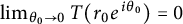


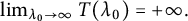
Point (2) says that
 $T(r_0e^{i\theta _0})$
approaches zero as
$T(r_0e^{i\theta _0})$
approaches zero as
 $\theta _0$
approaches zero, for “most” (but not necessarily all) nonzero
$\theta _0$
approaches zero, for “most” (but not necessarily all) nonzero
 $r_0$
inside the support of
$r_0$
inside the support of
 $\mu $
. The proposition allows us to extend the definition of T from
$\mu $
. The proposition allows us to extend the definition of T from
 $\mathbb C\setminus \operatorname {supp}(\mu )$
to all of
$\mathbb C\setminus \operatorname {supp}(\mu )$
to all of
 $\mathbb C\setminus \{0\}$
. This extension, however, may not be continuous.
$\mathbb C\setminus \{0\}$
. This extension, however, may not be continuous.
Proof We write the quantities
 $\tilde {p}_k$
in (3.10) in polar coordinates as
$\tilde {p}_k$
in (3.10) in polar coordinates as
 $$\begin{align*}\int_0^{\infty} \frac{\xi^k}{r_0^2+\xi^2-2\xi r_0\cos(\theta_0)}\,d\mu(\xi). \end{align*}$$
Since
 $\tilde {p}_k$
is an even function of
$\tilde {p}_k$
is an even function of
 $\theta _0$
, so is
$\theta _0$
, so is
 $T(r_0 e^{i\theta _0})$
. We therefore consider only the limit at
$T(r_0 e^{i\theta _0})$
. We therefore consider only the limit at
 $\theta _0$
approaches 0 from above. We then note that
$\theta _0$
approaches 0 from above. We then note that
 $\theta _0$
decreases toward zero, and the value of
$\theta _0$
decreases toward zero, and the value of
 $\tilde {p}_k$
increases. Thus, by the monotone convergence theorem,
$\tilde {p}_k$
increases. Thus, by the monotone convergence theorem,
 $$ \begin{align} \lim_{\theta_0\rightarrow 0}\tilde{p}_k=\int_0^{\infty}\frac{\xi^k}{(\xi-r_0)^2}\,d\mu(\xi). \end{align} $$
Point (1) of the proposition is then clear in the case that
 $\tilde {p}_0$
and
$\tilde {p}_0$
and
 $\tilde {p}_2$
are finite at
$\tilde {p}_2$
are finite at
 $\theta _0=0$
.
$\theta _0=0$
.
We then consider the case when at least one of
 $\tilde {p}_0$
and
$\tilde {p}_0$
and
 $\tilde {p}_2$
is infinite at
$\tilde {p}_2$
is infinite at
 $\theta _0=0$
, in which case,
$\theta _0=0$
, in which case,
 $\tilde {p}_0$
must be infinite. Now, since
$\tilde {p}_0$
must be infinite. Now, since
 $\mu \neq \delta _0$
, the value of
$\mu \neq \delta _0$
, the value of
 $\tilde {p}_2$
at
$\tilde {p}_2$
at
 $\theta _0 = 0$
is not zero. Furthermore, the value of
$\theta _0 = 0$
is not zero. Furthermore, the value of
 $\tilde {p}_2$
at any
$\tilde {p}_2$
at any
 $\theta _0$
is bounded below by its (positive) value at
$\theta _0$
is bounded below by its (positive) value at
 $\theta _0=0$
. Thus, by (3.24) and Lemma 3.9, the limit of
$\theta _0=0$
. Thus, by (3.24) and Lemma 3.9, the limit of
 $T(r_0 e^{i\theta _0})$
exists and is zero. We conclude that the limit in Point (1) of the proposition exists for all nonzero
$T(r_0 e^{i\theta _0})$
exists and is zero. We conclude that the limit in Point (1) of the proposition exists for all nonzero
 $r_0$
and that this limit is zero whenever the value of
$r_0$
and that this limit is zero whenever the value of
 $\tilde {p}_0$
at
$\tilde {p}_0$
at
 $\theta _0=0$
is infinite. But by Lemma 3.8,
$\theta _0=0$
is infinite. But by Lemma 3.8,
 $\tilde {p}_0=\infty $
(at
$\tilde {p}_0=\infty $
(at
 $\theta _0=0$
) for
$\theta _0=0$
) for
 $\mu $
-almost every nonzero value of
$\mu $
-almost every nonzero value of
 $r_0$
.
$r_0$
.
Finally, if
 $\lambda _0\rightarrow \infty $
, then the quantities
$\lambda _0\rightarrow \infty $
, then the quantities
 $\tilde p_0$
and
$\tilde p_0$
and
 $\tilde p_2$
in (3.23) tend to zero, so that by the second part of Lemma 3.9,
$\tilde p_2$
in (3.23) tend to zero, so that by the second part of Lemma 3.9,
 $T(\lambda _0)$
tends to
$T(\lambda _0)$
tends to
 $+\infty $
.
$+\infty $
.
Remark 3.11 In some cases, Point 2 of Proposition 3.10 will hold for every
 $r_0$
in the support of
$r_0$
in the support of
 $\mu $
. By examining the preceding proof, we see that this result will hold if
$\mu $
. By examining the preceding proof, we see that this result will hold if
 $$ \begin{align} \tilde p_0:=\int_0^\infty\frac{1}{(\xi-r_0)^2}\,d\mu(\xi)=\infty,\quad\forall r_0\in\operatorname{supp}(\mu). \end{align} $$
The condition (3.25) will hold if, for example,
 $\mu $
is a finite sum of measures, each of which is either a point mass or is supported on a closed interval with a Lebesgue density that is bounded away from zero on that interval.
$\mu $
is a finite sum of measures, each of which is either a point mass or is supported on a closed interval with a Lebesgue density that is bounded away from zero on that interval.
3.3 The domain and its properties
In the previous section, we obtain a lifetime
 $t_\ast $
of the solution to (3.4)–(3.5) and its limit T as
$t_\ast $
of the solution to (3.4)–(3.5) and its limit T as
 $\varepsilon _0 \rightarrow 0$
, where T is given outside the support of
$\varepsilon _0 \rightarrow 0$
, where T is given outside the support of
 $\mu $
by Definition 3.1. Also by Proposition 3.10, we can extend the domain of
$\mu $
by Definition 3.1. Also by Proposition 3.10, we can extend the domain of
 $T(\lambda _0)$
to every nonzero
$T(\lambda _0)$
to every nonzero
 $\lambda _0$
by letting
$\lambda _0$
by letting
 $\theta _0$
tend to
$\theta _0$
tend to
 $0$
(Figures 3 and 4).
$0$
(Figures 3 and 4).
Definition 3.2 For all
 $t>0$
, define a domain
$t>0$
, define a domain
 $\Sigma _t$
by
$\Sigma _t$
by
 $$\begin{align*}\Sigma_t = \{\lambda_0 \neq 0 : T(\lambda_0) < t\}.\end{align*}$$
By the last part of Proposition 3.10,
 $\Sigma _t$
is bounded for every
$\Sigma _t$
is bounded for every
 $t>0$
.
$t>0$
.
Corollary 3.12 For all
 $t>0$
, we have that
$t>0$
, we have that
 $\operatorname {supp}(\mu )\setminus \{0\}$
is contained in
$\operatorname {supp}(\mu )\setminus \{0\}$
is contained in
 $\overline {\Sigma }_t$
. In particular, if
$\overline {\Sigma }_t$
. In particular, if
 $0$
is in the support of
$0$
is in the support of
 $\mu $
but outside
$\mu $
but outside
 $\overline {\Sigma }_t$
, then
$\overline {\Sigma }_t$
, then
 $0$
is an isolated point mass of
$0$
is an isolated point mass of
 $\mu $
.
$\mu $
.
Proof By Point (2) of Proposition 3.10, the closed set
 $\overline \Sigma _t$
contains
$\overline \Sigma _t$
contains
 $\mu $
-almost every nonzero real number.
$\mu $
-almost every nonzero real number.
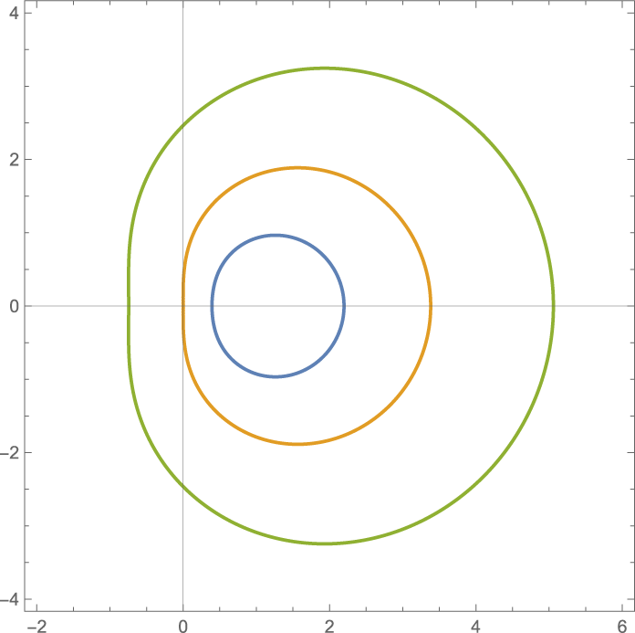
Figure 3: The domain
 $\overline {\Sigma }_t$
with
$\overline {\Sigma }_t$
with
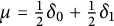 $\mu = \frac {1}{2}\delta _0 +\frac {1}{2}\delta _1$
, for
$\mu = \frac {1}{2}\delta _0 +\frac {1}{2}\delta _1$
, for
 $t=1$
(blue),
$t=1$
(blue),
 $t=2$
(orange), and
$t=2$
(orange), and
 $t=3$
(green).
$t=3$
(green).

Figure 4: The domain
 $\overline {\Sigma }_t$
with
$\overline {\Sigma }_t$
with
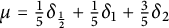 $\mu =\frac {1}{5}\delta _{\frac {1}{2}} +\frac {1}{5}\delta _1 + \frac {3}{5}\delta _{2}$
, for
$\mu =\frac {1}{5}\delta _{\frac {1}{2}} +\frac {1}{5}\delta _1 + \frac {3}{5}\delta _{2}$
, for
 $t =\frac {1}{10}$
(blue),
$t =\frac {1}{10}$
(blue),
 $t=\frac {1}{5}$
(orange), and
$t=\frac {1}{5}$
(orange), and
 $t=\frac {1}{2}$
(green).
$t=\frac {1}{2}$
(green).
The analogous domain to
 $\Sigma _t$
in [Reference Driver, Hall and Kemp10, Reference Ho and Zhong21] can be described as the set of points
$\Sigma _t$
in [Reference Driver, Hall and Kemp10, Reference Ho and Zhong21] can be described as the set of points
 $re^{i\theta }$
with
$re^{i\theta }$
with
 $1/r_t(\theta )<r<r_t(\theta )$
, for a certain function
$1/r_t(\theta )<r<r_t(\theta )$
, for a certain function
 $r_t$
. We now give a similar description of our domain, but with the roles of r and
$r_t$
. We now give a similar description of our domain, but with the roles of r and
 $\theta $
reversed.
$\theta $
reversed.
Definition 3.3 Let
 $\pi ^+$
be any number larger than
$\pi ^+$
be any number larger than
 $\pi $
. Define
$\pi $
. Define
 $\theta _t : (0, \infty ) \rightarrow [0, \pi ] \cup \{ \pi ^+\}$
by
$\theta _t : (0, \infty ) \rightarrow [0, \pi ] \cup \{ \pi ^+\}$
by
 $$ \begin{align*}\theta_t(r_0)= \inf\{\theta_0 \in (0, \pi] : T(r_0e^{i\theta_0}) \geq t\},\end{align*} $$
if the set is nonempty. Otherwise,
 $\theta _t(r_0) = \pi ^+$
.
$\theta _t(r_0) = \pi ^+$
.
Proposition 3.13 The domain
 $\Sigma _t$
in Definition 3.2 can be characterized as
$\Sigma _t$
in Definition 3.2 can be characterized as
 $$\begin{align*}\Sigma_t = \{r_0e^{i\theta_0} : r_0 \neq 0 \quad\text{and}\quad |\theta_0|<\theta_t(r_0)\}.\end{align*}$$
Figure 5 illustrates the meaning of three cases
 $\theta _t<\pi $
,
$\theta _t<\pi $
,
 $\theta _t=\pi $
, and
$\theta _t=\pi $
, and
 $\theta _t=\pi ^+$
. When
$\theta _t=\pi ^+$
. When
 $\theta _t(r_0)=\pi ^+$
, the entire circle of radius
$\theta _t(r_0)=\pi ^+$
, the entire circle of radius
 $r_0$
(centered at the origin) is contained in
$r_0$
(centered at the origin) is contained in
 $\Sigma _t$
. When
$\Sigma _t$
. When
 $\theta _t(r_0)=\pi $
, the entire circle of radius
$\theta _t(r_0)=\pi $
, the entire circle of radius
 $r_0$
, except the point on the negative real axis, is contained in
$r_0$
, except the point on the negative real axis, is contained in
 $\Sigma _t$
.
$\Sigma _t$
.

Figure 5: A portion of the domain
 $\Sigma _t$
with
$\Sigma _t$
with
 $\mu =\delta _1$
and
$\mu =\delta _1$
and
 $t=4.02$
.
$t=4.02$
.
The following result is the key to proving Proposition 3.13.
Lemma 3.14 For each
 $\lambda _0$
with
$\lambda _0$
with
 $\Im (\lambda _0) \neq 0$
, the sign of
$\Im (\lambda _0) \neq 0$
, the sign of
 $\partial T(\lambda _0)/\partial \theta $
is the same as the sign of
$\partial T(\lambda _0)/\partial \theta $
is the same as the sign of
 $\Im (\lambda _0)$
.
$\Im (\lambda _0)$
.
The lemma says that T increases as we move away from the positive x-axis in the radial direction.
Proof We use the subscript notation
 $f_\theta $
for the partial derivative of a function f in the angular direction. Since
$f_\theta $
for the partial derivative of a function f in the angular direction. Since
 $T(\overline {\lambda _0})=T(\lambda _0)$
, we see that
$T(\overline {\lambda _0})=T(\lambda _0)$
, we see that
 $T(r_0 e^{i\theta })$
is an even function of
$T(r_0 e^{i\theta })$
is an even function of
 $\theta $
. It therefore suffices to show that
$\theta $
. It therefore suffices to show that
 $T_\theta $
is positive when
$T_\theta $
is positive when
 $\Im (\lambda _0)$
is positive. Let
$\Im (\lambda _0)$
is positive. Let
 $$ \begin{align*}R = \frac{\tilde{p}_0r_0^2}{\tilde{p}_2}.\end{align*} $$
Note that T can be computed as
 $$ \begin{align*}T(r_0e^{i\theta}) = \frac{1}{\tilde{p}_2(R-1)}\log(R).\end{align*} $$
We first make a preliminary calculation:
 $$ \begin{align*} T_\theta = \left(\frac{1}{\tilde{p}_2 (R-1)}\right)_\theta \log(R)+\frac{1}{\tilde{p}_2(R-1)}\frac{R_\theta}{R}. \end{align*} $$
We then use the inequality
 $$ \begin{align}1-1/x\leq \log x \leq x-1,\end{align} $$
which may be proved by writing
 $\log x$
as the integral of
$\log x$
as the integral of
 $1/y$
from 1 to x and then bounding
$1/y$
from 1 to x and then bounding
 $1/y$
between 1 and
$1/y$
between 1 and
 $1/x$
(for
$1/x$
(for
 $x<1$
) and between
$x<1$
) and between
 $1/x$
and 1 (for
$1/x$
and 1 (for
 $x>1$
).
$x>1$
).
In the case that
 $\left (\frac {1}{\tilde {p}_2 (R-1)}\right )_\theta $
is positive, we use the first inequality in (3.26) to give
$\left (\frac {1}{\tilde {p}_2 (R-1)}\right )_\theta $
is positive, we use the first inequality in (3.26) to give
 $$ \begin{align*} T_\theta\geq \left(\frac{1}{\tilde{p}_2 (R-1)}\right)_\theta (1-1/R)+\frac{1}{\tilde{p}_2(R-1)}\frac{R_\theta}{R}. \end{align*} $$
Simplifying this result gives
 $$ \begin{align*} T_\theta \geq -\frac{(\tilde{p}_2)_\theta}{\tilde{p}_2^2R}. \end{align*} $$
But
 $$ \begin{align*} (\tilde{p}_2)_\theta = -\Im (\lambda_0)\int_0^\infty \frac{\xi^3}{(\xi^2 -2\xi r_0\cos \theta + r_0^2)^2} \,d\mu(\xi). \end{align*} $$
Thus,
 $T_\theta $
is positive when
$T_\theta $
is positive when
 $\Im (\lambda _0)$
is positive and we are done in this case.
$\Im (\lambda _0)$
is positive and we are done in this case.
In the case that
 $\left (\frac {1}{\tilde {p}_2 (R-1)}\right )_\theta $
is negative, we use the second inequality in (3.26) to give
$\left (\frac {1}{\tilde {p}_2 (R-1)}\right )_\theta $
is negative, we use the second inequality in (3.26) to give
 $$ \begin{align*} T_\theta\geq \left(\frac{1}{\tilde{p}_2 (R-1)}\right)_\theta (R-1)+\frac{1}{\tilde{p}_2(R-1)}\frac{R_\theta}{R}. \end{align*} $$
Simplifying this result gives
 $$ \begin{align*} T_\theta &\geq - \frac{[(\tilde{p}_2)_\theta R+\tilde{p}_2R_\theta]}{\tilde{p}_2^2 R} \\ &= -\frac{(\tilde{p}_2R)_\theta}{\tilde{p}_2^2R}. \end{align*} $$
But since
 $\tilde {p}_2R = \tilde {p}_0r_0^2$
, we compute that
$\tilde {p}_2R = \tilde {p}_0r_0^2$
, we compute that
 $$ \begin{align*} [\tilde{p}_2R]_\theta = -\Im (\lambda_0)\int_0^\infty \frac{r_0^2\xi}{(\xi^2 -2\xi r_0\cos \theta + r_0^2)^2} \,d\mu(\xi). \end{align*} $$
Thus,
 $T_\theta $
is positive when
$T_\theta $
is positive when
 $\Im (\lambda _0)$
is positive and we are done in this case.
$\Im (\lambda _0)$
is positive and we are done in this case.
Proof of Proposition 3.13.
Suppose that
 $\lambda _0 =r_0e^{i\theta _0}$
with
$\lambda _0 =r_0e^{i\theta _0}$
with
 $\theta _0 \neq 0$
. Then, by the monotonicity of
$\theta _0 \neq 0$
. Then, by the monotonicity of
 $T(r_0e^{i\theta _0})$
with respect to
$T(r_0e^{i\theta _0})$
with respect to
 $\theta _0$
(Lemma 3.14),
$\theta _0$
(Lemma 3.14),
 $|\theta _0| < \theta _t(r_0)$
if and only if
$|\theta _0| < \theta _t(r_0)$
if and only if
 $T(\lambda _0) <t$
. here
$T(\lambda _0) <t$
. here
Proposition 3.15 For
 $t>0$
,
$t>0$
,
 $\Sigma _t$
is open.
$\Sigma _t$
is open.
To show that
 $\Sigma _t$
is open, we first show that
$\Sigma _t$
is open, we first show that
 $\theta _t$
is continuous in the following sense.
$\theta _t$
is continuous in the following sense.
Lemma 3.16 Let
 $r_0>0$
. We have:
$r_0>0$
. We have:
-
(1) If
$\theta _t(r_0) = \pi ^+$
, there exists a neighborhood B of
$r_0$
such that
$\theta _t(s) = \pi ^+$
for all
$s \in B$
. -
(2) If
$\theta _t(r_0) = \pi $
, then for all
$\varepsilon>0$
, there exists a neighborhood B of
$r_0$
such that
$\theta _t(s) \in (\pi -\varepsilon ,\pi ]$
or
$\theta _t(s) = \pi ^+$
for all
$s \in B$
. -
(3) If
$\theta _t(r_0) < \pi $
, then for all
$\varepsilon>0$
, there exists a neighborhood B of
$r_0$
such that
$|\theta _t(r_0) - \theta _t(s)| <\varepsilon $
for all
$s \in B_3$
.


Proof The function T in Definition 3.1 is continuous outside
 $\operatorname {supp}(\mu )$
and, in particular, outside
$\operatorname {supp}(\mu )$
and, in particular, outside
 $[0, \infty )$
.
$[0, \infty )$
.
First, assume
 $\theta _t(r_0) = \pi ^+$
. Note that by monotonicity of
$\theta _t(r_0) = \pi ^+$
. Note that by monotonicity of
 $T(r_0e^{i\theta _0})$
with respect to
$T(r_0e^{i\theta _0})$
with respect to
 $\theta _0$
(Lemma 3.14),
$\theta _0$
(Lemma 3.14),
 $\theta _t(r_0) = \pi ^+$
if and only if
$\theta _t(r_0) = \pi ^+$
if and only if
 $T(r_0e^{i\pi }) <t$
. By the continuity of T, there exists a neighborhood B of
$T(r_0e^{i\pi }) <t$
. By the continuity of T, there exists a neighborhood B of
 $r_0$
such that
$r_0$
such that
 $T(s e^{i\pi }) <t$
for all
$T(s e^{i\pi }) <t$
for all
 $s \in B_1$
. Hence,
$s \in B_1$
. Hence,
 $\theta _t(s) = \pi ^+$
for all
$\theta _t(s) = \pi ^+$
for all
 $s \in B$
.
$s \in B$
.
Next, assume
 $\theta _t(r_0) = \pi $
. Let
$\theta _t(r_0) = \pi $
. Let
 $\varepsilon>0$
, where it is harmless to assume
$\varepsilon>0$
, where it is harmless to assume
 $\varepsilon <\pi $
. Then, by the definition of
$\varepsilon <\pi $
. Then, by the definition of
 $\theta _t$
, we must have
$\theta _t$
, we must have
 $T(r_0 e^{i(\pi -\varepsilon )})<t$
. Thus, by the continuity of T, there is some neighborhood B of
$T(r_0 e^{i(\pi -\varepsilon )})<t$
. Thus, by the continuity of T, there is some neighborhood B of
 $r_0$
such that
$r_0$
such that
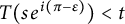 $T(s e^{i(\pi -\varepsilon )})<t$
for all
$T(s e^{i(\pi -\varepsilon )})<t$
for all
 $s\in B$
. Finally, by the monotonicity of T, we must have
$s\in B$
. Finally, by the monotonicity of T, we must have
 $\theta _t(s)>\pi -\varepsilon $
for
$\theta _t(s)>\pi -\varepsilon $
for
 $s\in B$
, meaning that either
$s\in B$
, meaning that either
 $\theta _t(s)\in (\pi -\varepsilon ,\pi ]$
or
$\theta _t(s)\in (\pi -\varepsilon ,\pi ]$
or
 $\theta _t(s)=\pi ^+$
.
$\theta _t(s)=\pi ^+$
.
Finally, assume
 $\theta _t(r_0) < \pi .$
Let
$\theta _t(r_0) < \pi .$
Let
 $\varepsilon>0$
, where it is harmless to assume that
$\varepsilon>0$
, where it is harmless to assume that
 $\theta _t(r_0)+\varepsilon <\pi $
and (in the case
$\theta _t(r_0)+\varepsilon <\pi $
and (in the case
 $\theta _t(r_0)>0$
) that
$\theta _t(r_0)>0$
) that
 $\theta _t(r_0)-\varepsilon>0$
. Then, by monotonicity of T, we have
$\theta _t(r_0)-\varepsilon>0$
. Then, by monotonicity of T, we have
 $T(r_0e^{i(\theta _t(r_0)+\varepsilon )})> t$
. Since T is continuous, there exists a neighborhood U of
$T(r_0e^{i(\theta _t(r_0)+\varepsilon )})> t$
. Since T is continuous, there exists a neighborhood U of
 $r_0$
such that
$r_0$
such that
 $$ \begin{align*}T(s e^{i(\theta_t(r_0)+\varepsilon)})> t, \quad \forall s \in U.\end{align*} $$
Hence,
 $\theta _t(s) \leq \theta _t(r_0) + \varepsilon $
, for all
$\theta _t(s) \leq \theta _t(r_0) + \varepsilon $
, for all
 $s \in U.$
In the case
 $\theta _t(r_0) =0$
, we may then take
$\theta _t(r_0) =0$
, we may then take
 $B=U$
. In the case
$B=U$
. In the case
 $\theta _t(r_0) \neq 0$
, the monotonicity of T shows that
$\theta _t(r_0) \neq 0$
, the monotonicity of T shows that
 $T(r_0 e^{i(\theta _0(r_0)-\varepsilon )}) < t.$
Since T is continuous, there exists a neighborhood V of
$T(r_0 e^{i(\theta _0(r_0)-\varepsilon )}) < t.$
Since T is continuous, there exists a neighborhood V of
 $r_0$
such that
$r_0$
such that
 $$ \begin{align*}T(s e^{i(\theta_0(r_0)-\varepsilon)}) < t, \quad \forall s \in V.\end{align*} $$
Hence,
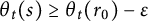 $\theta _t(s) \geq \theta _t(r_0) - \varepsilon $
, for all
$\theta _t(s) \geq \theta _t(r_0) - \varepsilon $
, for all
 $s \in V.$
Thus, we may take
$s \in V.$
Thus, we may take
 $B=U\cap V$
.
$B=U\cap V$
.
Proof of Proposition 3.15.
By Proposition 3.13,
 $\Sigma _t$
is the set
$\Sigma _t$
is the set
 $r_0 e^{i\theta _0}$
with
$r_0 e^{i\theta _0}$
with
 $r_0\neq 0$
and
$r_0\neq 0$
and
 $\vert \theta _0\vert <\theta _t(r_0)$
. Fix
$\vert \theta _0\vert <\theta _t(r_0)$
. Fix
 $r_0e^{i\theta _0}\in \Sigma _t$
. If
$r_0e^{i\theta _0}\in \Sigma _t$
. If
 $\theta _t(r_0)=\pi ^+$
, then by Point (1) of Lemma 3.16, there is a neighborhood B of
$\theta _t(r_0)=\pi ^+$
, then by Point (1) of Lemma 3.16, there is a neighborhood B of
 $r_0$
on which
$r_0$
on which
 $\theta _t=\pi ^+$
, in which case all
$\theta _t=\pi ^+$
, in which case all
 $s e^{i\theta }$
with
$s e^{i\theta }$
with
 $s\in B$
belong to
$s\in B$
belong to
 $\Sigma _t$
.
$\Sigma _t$
.
If
 $\theta _t(r_0)\neq \pi ^+$
, set
$\theta _t(r_0)\neq \pi ^+$
, set
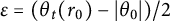 $\varepsilon =(\theta _t(r_0)-\vert \theta _0\vert )/2$
. Then, by Points (2) and (3) of Lemma 3.16, there is a neighborhood B of
$\varepsilon =(\theta _t(r_0)-\vert \theta _0\vert )/2$
. Then, by Points (2) and (3) of Lemma 3.16, there is a neighborhood B of
 $r_0$
on which
$r_0$
on which
 $$ \begin{align*}\theta_t(s)>\theta_t(r_0)-\varepsilon=\theta_0+\varepsilon.\end{align*} $$
Then, all
 $s e^{i\theta }$
with
$s e^{i\theta }$
with
 $s\in B$
and
$s\in B$
and
 $\theta $
within
$\theta $
within
 $\varepsilon $
of
$\varepsilon $
of
 $\theta _0$
are in
$\theta _0$
are in
 $\Sigma _t$
.
$\Sigma _t$
.
Proposition 3.17 For nonzero
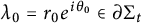 $\lambda _0=r_0 e^{i\theta _0} \in \partial \Sigma _t$
, we have:
$\lambda _0=r_0 e^{i\theta _0} \in \partial \Sigma _t$
, we have:
-
(1)
$\theta _t(r_0) \neq \pi ^+$
and
$\lambda _0 = r_0 e^{i\theta _t(r_0)}$
; -
(2)
$T(\lambda _0) \geq t$
; -
(3) if
$\theta _0 \neq 0$
or
$\theta _0=0$
but
$r_0\notin \operatorname {supp}(\mu )$
, then
$T(\lambda _0) =t$
.

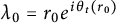


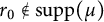

Furthermore, if
 $\arg (\lambda _0) \neq 0$
and
$\arg (\lambda _0) \neq 0$
and
 $T(\lambda _0) =t$
, then
$T(\lambda _0) =t$
, then
 $\lambda _0 \in \partial \Sigma _t$
.
$\lambda _0 \in \partial \Sigma _t$
.
Figure 6 shows an example in which
 $T(\lambda _0)>t$
at a boundary point of
$T(\lambda _0)>t$
at a boundary point of
 $\Sigma _t$
. In the example,
$\Sigma _t$
. In the example,
 $T(\lambda _0)=0$
for all
$T(\lambda _0)=0$
for all
 $\lambda _0\in (1,2]$
but
$\lambda _0\in (1,2]$
but
 $T(1)>0$
, because the momenta
$T(1)>0$
, because the momenta
 $\tilde p_0$
and
$\tilde p_0$
and
 $\tilde p_2$
from (3.23) are infinite on
$\tilde p_2$
from (3.23) are infinite on
 $(0, 2]$
but finite at 1.
$(0, 2]$
but finite at 1.

Figure 6: The domain
 $\overline \Sigma _t $
with
$\overline \Sigma _t $
with
 $d\mu (\xi )=1_{[1,2]}(\xi -1)^2/3\,d\xi $
for
$d\mu (\xi )=1_{[1,2]}(\xi -1)^2/3\,d\xi $
for
 $t=1/2$
(blue) and
$t=1/2$
(blue) and
 $t=1$
(orange). The function T has a value of approximately 1.91 at the point 1, which is on the boundary of both domains.
$t=1$
(orange). The function T has a value of approximately 1.91 at the point 1, which is on the boundary of both domains.
Remark 3.18 If the condition (3.25) in Remark 3.11 holds, then
 $T\equiv 0$
on
$T\equiv 0$
on
 $\operatorname {supp}(\mu )\setminus \{0\}$
, so that
$\operatorname {supp}(\mu )\setminus \{0\}$
, so that
 $\operatorname {supp}(\mu )\setminus \{0\}$
is contained in the open set
$\operatorname {supp}(\mu )\setminus \{0\}$
is contained in the open set
 $\Sigma _t$
for every
$\Sigma _t$
for every
 $t>0$
. In that case, we can conclude that
$t>0$
. In that case, we can conclude that
 $T(\lambda _0)=t$
for every nonzero
$T(\lambda _0)=t$
for every nonzero
 $\lambda _0$
in the boundary of
$\lambda _0$
in the boundary of
 $\Sigma _t$
.
$\Sigma _t$
.
Proof Fix
 $\lambda _0=r_0 e^{i\theta _0}$
, with
$\lambda _0=r_0 e^{i\theta _0}$
, with
 $-\pi <\theta \leq \pi $
, belonging to
$-\pi <\theta \leq \pi $
, belonging to
 $\partial \Sigma _t\setminus \{0\}$
Then,
$\partial \Sigma _t\setminus \{0\}$
Then,
 $\lambda _0$
cannot be in the open set
$\lambda _0$
cannot be in the open set
 $\Sigma _t$
. Since
$\Sigma _t$
. Since
 $T(\bar \lambda _0)=T(\lambda _0)$
, we can assume that
$T(\bar \lambda _0)=T(\lambda _0)$
, we can assume that
 $\lambda _0$
is in the closed upper half plane. Then,
$\lambda _0$
is in the closed upper half plane. Then,
 $\theta _t(r_0)$
cannot be
$\theta _t(r_0)$
cannot be
 $\pi ^+$
or
$\pi ^+$
or
 $\lambda _0$
would be in
$\lambda _0$
would be in
 $\Sigma _t$
. If
$\Sigma _t$
. If
 $\theta _0=0$
, then
$\theta _0=0$
, then
 $\theta _t(r_0)$
must be zero, or
$\theta _t(r_0)$
must be zero, or
 $\lambda _0$
would be in
$\lambda _0$
would be in
 $\Sigma _t$
. If
$\Sigma _t$
. If
 $0<\theta _0\leq \pi $
, then
$0<\theta _0\leq \pi $
, then
 $\theta _0$
cannot be less then
$\theta _0$
cannot be less then
 $\theta _t(r_0)$
or
$\theta _t(r_0)$
or
 $\lambda _0$
would be in
$\lambda _0$
would be in
 $\Sigma _t$
. But also
$\Sigma _t$
. But also
 $\theta _0$
cannot be greater than
$\theta _0$
cannot be greater than
 $\theta _t(r_0)$
or
$\theta _t(r_0)$
or
 $\theta _t(r_0)$
would be less than
$\theta _t(r_0)$
would be less than
 $\pi $
– and then by the continuity of
$\pi $
– and then by the continuity of
 $\theta _t$
, there would be a neighborhood of
$\theta _t$
, there would be a neighborhood of
 $\lambda _0$
outside
$\lambda _0$
outside
 $\Sigma _t$
. In that case,
$\Sigma _t$
. In that case,
 $\lambda _0$
could not be in
$\lambda _0$
could not be in
 $\partial \Sigma _t$
. Thus, in all cases,
$\partial \Sigma _t$
. Thus, in all cases,
 $\theta _0=\theta _t(r_0)$
, establishing the first part of the proposition.
$\theta _0=\theta _t(r_0)$
, establishing the first part of the proposition.
For the second part,
 $T(\lambda _0)$
cannot be less than t or
$T(\lambda _0)$
cannot be less than t or
 $\lambda _0$
would be in
$\lambda _0$
would be in
 $\Sigma _t$
. For the third part, the assumptions ensure that
$\Sigma _t$
. For the third part, the assumptions ensure that
 $\lambda _0$
is not in
$\lambda _0$
is not in
 $\operatorname {supp}(\mu )$
, in which case, T is continuous at
$\operatorname {supp}(\mu )$
, in which case, T is continuous at
 $\lambda _0$
. Then, since
$\lambda _0$
. Then, since
 $\lambda _0$
is a limit of points with
$\lambda _0$
is a limit of points with
 $T<t$
, we have
$T<t$
, we have
 $T(\lambda _0)\leq t$
(and also
$T(\lambda _0)\leq t$
(and also
 $T(\lambda _0)\geq t$
).
$T(\lambda _0)\geq t$
).
Lastly, let
 $\lambda _0$
be such that
$\lambda _0$
be such that
 $T(\lambda _0) =t$
and
$T(\lambda _0) =t$
and
 $\arg (\lambda _0) \neq 0$
. Then,
$\arg (\lambda _0) \neq 0$
. Then,
 $\lambda _0$
is, by definition, not in
$\lambda _0$
is, by definition, not in
 $\Sigma _t$
. But
$\Sigma _t$
. But
 $\lambda _0$
must be in the closure of
$\lambda _0$
must be in the closure of
 $\Sigma _t$
, by the monotonicity of T with respect to
$\Sigma _t$
, by the monotonicity of T with respect to
 $\theta $
. Thus,
$\theta $
. Thus,
 $\lambda _0$
must be in the boundary of
$\lambda _0$
must be in the boundary of
 $\Sigma _t$
.
$\Sigma _t$
.
3.4 The “outside the domain” calculation
In this section, we will always take
 $\lambda _0$
outside
$\lambda _0$
outside
 $\operatorname {supp}(\mu )$
, in which case, the initial momenta in (3.6)–(3.8) will have finite limits as
$\operatorname {supp}(\mu )$
, in which case, the initial momenta in (3.6)–(3.8) will have finite limits as
 $\varepsilon _0$
tends to zero. We use the notation
$\varepsilon _0$
tends to zero. We use the notation
 $$ \begin{align*}\mu_t=\text{ Brown measure of }xb_t.\end{align*} $$
Our aim is to calculate
 $$\begin{align*}s_t(\lambda) = \lim_{\varepsilon \rightarrow 0^+} S(t,\lambda,\varepsilon),\end{align*}$$
using the Hamilton–Jacobi formula in Theorem 3.4. Our approach is to choose “good” initial conditions
 $\lambda _0$
and
$\lambda _0$
and
 $\varepsilon _0$
in the Hamiltonian system (3.4)–(3.5) (with initial momenta given by (3.6)–(3.8)) so that
$\varepsilon _0$
in the Hamiltonian system (3.4)–(3.5) (with initial momenta given by (3.6)–(3.8)) so that
 $\lambda (t)=\lambda $
and
$\lambda (t)=\lambda $
and
 $\varepsilon (t)=0$
.
$\varepsilon (t)=0$
.
Now, in light of (3.21), we see that if
 $\varepsilon _0$
is very small, then
$\varepsilon _0$
is very small, then
 $\varepsilon (s)$
will be positive but small for
$\varepsilon (s)$
will be positive but small for
 $0\leq s\leq t$
, provided that the solution of the system (3.4)–(3.5) exists up to time t. Furthermore, the argument
$0\leq s\leq t$
, provided that the solution of the system (3.4)–(3.5) exists up to time t. Furthermore, the argument
 $\theta =\arg (\lambda )$
is a constant of motion. Finally, by (3.12), if
$\theta =\arg (\lambda )$
is a constant of motion. Finally, by (3.12), if
 $\varepsilon _0$
is small (so that
$\varepsilon _0$
is small (so that
 $\varepsilon (s)$
is small for
$\varepsilon (s)$
is small for
 $s<t$
), then
$s<t$
), then
 $\vert \lambda (s)\vert $
will be close to
$\vert \lambda (s)\vert $
will be close to
 $\vert \lambda _0\vert $
for
$\vert \lambda _0\vert $
for
 $s<t$
.
$s<t$
.
We therefore propose to take
 $\lambda _0=\lambda $
and
$\lambda _0=\lambda $
and
 $\varepsilon _0\rightarrow 0$
, with the result that
$\varepsilon _0\rightarrow 0$
, with the result that
 $$\begin{align*}\lambda(t) \equiv \lambda \quad \text{and} \quad \varepsilon(t) \equiv 0.\end{align*}$$
Now, we recall the Hamilton–Jacobi formula in (3.11), which reads (after using (3.9)):
 $$ \begin{align}S(t,\lambda(t),\varepsilon(t)) = S(0,\lambda_0,\varepsilon_0) + \varepsilon_0p_0p_2t +\log|\lambda(t)| - \log|\lambda_0|.\end{align} $$
Suppose we can simply let
 $\varepsilon _0 \rightarrow 0$
. Then, the second term on the right-hand side of (3.27) will be zero for
$\varepsilon _0 \rightarrow 0$
. Then, the second term on the right-hand side of (3.27) will be zero for
 $\lambda _0\notin \operatorname {supp}(\mu )$
, because
$\lambda _0\notin \operatorname {supp}(\mu )$
, because
 $p_0p_2$
remains finite. Furthermore, since
$p_0p_2$
remains finite. Furthermore, since
 $\lambda (t)=\lambda _0$
, the last two terms in the Hamilton–Jacobi formula cancel, leaving us with
$\lambda (t)=\lambda _0$
, the last two terms in the Hamilton–Jacobi formula cancel, leaving us with
 $$\begin{align*}S(t,\lambda,0)=S(0,\lambda,0)=\int_0^{\infty}\log(|\xi-\lambda|^2)\,d\mu(\xi). \end{align*}$$
If the preceding formula holds on any open set U outside the support of
 $\mu $
, then
$\mu $
, then
 $S(0,\lambda ,0)$
will be harmonic there, meaning that the Brown measure
$S(0,\lambda ,0)$
will be harmonic there, meaning that the Brown measure
 $\mu _t$
is zero on U. We note, however, that in order for the preceding strategy to work, the lifetime of the solution to (3.4) and (3.5) must remain greater than t in the limit
$\mu _t$
is zero on U. We note, however, that in order for the preceding strategy to work, the lifetime of the solution to (3.4) and (3.5) must remain greater than t in the limit
 $\varepsilon _0\rightarrow 0$
. We may then hope to carry out the strategy for
$\varepsilon _0\rightarrow 0$
. We may then hope to carry out the strategy for
 $\lambda _0$
outside the closed domain
$\lambda _0$
outside the closed domain
 $\overline \Sigma _t$
, as the following theorem confirms.
$\overline \Sigma _t$
, as the following theorem confirms.
Theorem 3.19 Fix a pair
 $(t,\lambda )$
with
$(t,\lambda )$
with
 $\lambda $
outside
$\lambda $
outside
 $\overline {\Sigma }_t$
. Then,
$\overline {\Sigma }_t$
. Then,
 $$ \begin{align*}s_t(\lambda) := \lim_{\varepsilon_0 \rightarrow 0^+} S(t,\lambda,\varepsilon)= \int_0^{\infty}\log(|\xi-\lambda|^2)\,d\mu(\xi).\end{align*} $$
In particular, the Brown measure
 $\mu _t$
of
$\mu _t$
of
 $xb_t$
is zero outside of
$xb_t$
is zero outside of
 $\overline {\Sigma }_t$
except possibly at the origin. Furthermore, if
$\overline {\Sigma }_t$
except possibly at the origin. Furthermore, if
 $0\notin \overline {\Sigma }_t$
, then
$0\notin \overline {\Sigma }_t$
, then
 $$\begin{align*}\mu_t(\{0\}) = \mu(\{0\}).\end{align*}$$
The theorem tells us that the log potential of the Brown measure
 $\mu _t$
agrees outside
$\mu _t$
agrees outside
 $\Sigma _t$
with the log potential of the law
$\Sigma _t$
with the log potential of the law
 $\mu $
of the self-adjoint element x. (This does not, however, mean that
$\mu $
of the self-adjoint element x. (This does not, however, mean that
 $\mu _t=\mu $
.)
$\mu _t=\mu $
.)
We now begin working toward the proof of Theorem 3.19. If
 $\lambda _0$
is outside
$\lambda _0$
is outside
 $\Sigma _t$
, then by definition,
$\Sigma _t$
, then by definition,
 $T(\lambda _0)$
must be at least t. But if
$T(\lambda _0)$
must be at least t. But if
 $T(\lambda _0)=t$
then by the last part of Proposition 3.17,
$T(\lambda _0)=t$
then by the last part of Proposition 3.17,
 $\lambda _0$
must be in the boundary of
$\lambda _0$
must be in the boundary of
 $\Sigma _t$
, provided that
$\Sigma _t$
, provided that
 $\lambda _0$
is not on the positive real axis. That is,
$\lambda _0$
is not on the positive real axis. That is,
 $T(\lambda _0)>t$
for all
$T(\lambda _0)>t$
for all
 $\lambda _0 \notin \overline {\Sigma }_t \cup [0, \infty )$
. Thus, for such
$\lambda _0 \notin \overline {\Sigma }_t \cup [0, \infty )$
. Thus, for such
 $\lambda _0$
, the lifetime
$\lambda _0$
, the lifetime
 $t_\ast (\lambda _0,\varepsilon _0)$
will be greater than t for all sufficiently small
$t_\ast (\lambda _0,\varepsilon _0)$
will be greater than t for all sufficiently small
 $\varepsilon _0$
. For
$\varepsilon _0$
. For
 $\lambda _0 \notin \overline {\Sigma }_t \cup [0, \infty )$
and
$\lambda _0 \notin \overline {\Sigma }_t \cup [0, \infty )$
and
 $\varepsilon _0>0$
, we define for each
$\varepsilon _0>0$
, we define for each
 $t>0$
a map
$t>0$
a map
 $U_t$
by
$U_t$
by
 $$ \begin{align} U_t(\lambda_0,\varepsilon_0) = (\lambda(t;\lambda_0,\varepsilon_0),\varepsilon(t;\lambda_0,\varepsilon_0)),\end{align} $$
where
 $\lambda (t;\lambda _0,\varepsilon _0)$
and
$\lambda (t;\lambda _0,\varepsilon _0)$
and
 $\varepsilon (t;\lambda _0,\varepsilon _0)$
denote the
$\varepsilon (t;\lambda _0,\varepsilon _0)$
denote the
 $\lambda $
- and
$\lambda $
- and
 $\varepsilon $
-components of the solution of (3.4) and (3.5) with the given initial conditions. We note by Theorem 3.6 that this map makes sense even if
$\varepsilon $
-components of the solution of (3.4) and (3.5) with the given initial conditions. We note by Theorem 3.6 that this map makes sense even if
 $\varepsilon _0$
is slightly negative.
$\varepsilon _0$
is slightly negative.
We will evaluate the derivative of this map at
 $(\lambda _0,\varepsilon _0) = (\lambda _0,0)$
.
$(\lambda _0,\varepsilon _0) = (\lambda _0,0)$
.
Lemma 3.20 For all
 $\lambda _0\notin \overline {\Sigma }_t \cup [0, \infty )$
, the Jacobian of
$\lambda _0\notin \overline {\Sigma }_t \cup [0, \infty )$
, the Jacobian of
 $U_t$
at
$U_t$
at
 $(\lambda _0,0)$
has the form:
$(\lambda _0,0)$
has the form:
 $$ \begin{align*}U_t^{'}(\lambda_0,0) = \begin{pmatrix} I_{2\times2} & \frac{\partial \lambda}{\partial \varepsilon_0}(t;\lambda_0,0) \\ 0 & \frac{\partial \varepsilon}{\partial \varepsilon_0}(t;\lambda_0,0) \end{pmatrix}\end{align*} $$
with
 $\frac {\partial \varepsilon }{\partial \varepsilon _0}(t;\lambda _0,0)> 0.$
Proof (Similar to Lemma 6.3 in [Reference Driver, Hall and Kemp10]) Note that if
 $\varepsilon _0 = 0$
, then
$\varepsilon _0 = 0$
, then
 $\varepsilon (t) \equiv 0$
and
$\varepsilon (t) \equiv 0$
and
 $\lambda (t) \equiv \lambda _0$
. Thus,
$\lambda (t) \equiv \lambda _0$
. Thus,
 $U_t(\lambda _0,0) = (\lambda _0,0)$
. Then, we only need to show that
$U_t(\lambda _0,0) = (\lambda _0,0)$
. Then, we only need to show that
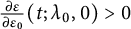 $\frac {\partial \varepsilon }{\partial \varepsilon _0}(t;\lambda _0,0)> 0$
. From Lemma 3.5, we have
$\frac {\partial \varepsilon }{\partial \varepsilon _0}(t;\lambda _0,0)> 0$
. From Lemma 3.5, we have
 $$ \begin{align*} \frac{\partial \varepsilon}{\partial \varepsilon_0}(t;\lambda_0,0) &= \frac{1}{p_\varepsilon(t)^2} p_0^2e^{-Ct} + \varepsilon_0 \frac{\partial}{\partial \varepsilon_0}\left[\frac{1}{p_\varepsilon(t)^2} p_0^2e^{-Ct}\right]\bigg\vert_{\varepsilon_0 = 0}\\ &=\frac{1}{p_\varepsilon(t)^2} p_0^2e^{-Ct}>0, \end{align*} $$
as claimed.
Now, we are ready to prove our main result.
Proof
We first establish the result for
 $\lambda \notin \overline {\Sigma }_t \cup [0, \infty )$
. We take
$\lambda \notin \overline {\Sigma }_t \cup [0, \infty )$
. We take
 $\lambda _0=\lambda $
in Lemma 3.20. Then, by the inverse function theorem, the map
$\lambda _0=\lambda $
in Lemma 3.20. Then, by the inverse function theorem, the map
 $U_t$
in (3.28) has a local inverse near
$U_t$
in (3.28) has a local inverse near
 $U_t(\lambda ,0)=(\lambda ,0)$
.
$U_t(\lambda ,0)=(\lambda ,0)$
.
Now, the inverse of the matrix in Lemma 3.20 will have a positive entry in the bottom right corner; that is,
 $U_t^{-1}$
has the property that
$U_t^{-1}$
has the property that
 $\partial \varepsilon _0/\partial \varepsilon>0$
. Thus, the
$\partial \varepsilon _0/\partial \varepsilon>0$
. Thus, the
 $\varepsilon _0$
-component of
$\varepsilon _0$
-component of
 $U_t^{-1}(\lambda ,\varepsilon )$
will be positive for
$U_t^{-1}(\lambda ,\varepsilon )$
will be positive for
 $\varepsilon $
small and positive. In that case, the solution of the Hamiltonian system (3.4)–(3.5) will have
$\varepsilon $
small and positive. In that case, the solution of the Hamiltonian system (3.4)–(3.5) will have
 $\varepsilon (u)>0$
up to the blow-up time. In turn, the blow-up time with initial conditions
$\varepsilon (u)>0$
up to the blow-up time. In turn, the blow-up time with initial conditions
 $(\lambda _0,\varepsilon _0)=U_t^{-1}(\lambda ,\varepsilon )$
will exceed t for
$(\lambda _0,\varepsilon _0)=U_t^{-1}(\lambda ,\varepsilon )$
will exceed t for
 $\varepsilon $
close to 0.
$\varepsilon $
close to 0.
We now let “HJ” denote the quantity on the right-hand side of the Hamilton–Jacobi formula (3.27):
 $$ \begin{align} \mathrm{HJ}(t,\lambda_0,\varepsilon_0) = S(0,\lambda_0,\varepsilon_0) + \varepsilon_0p_0p_2t +\log|\lambda(t)| - \log|\lambda_0| .\end{align} $$
If
 $\varepsilon $
is small and positive, the Hamilton–Jacobi formula (3.27) tells us that
$\varepsilon $
is small and positive, the Hamilton–Jacobi formula (3.27) tells us that
 $$ \begin{align} S(t,\lambda,\varepsilon) = \mathrm{HJ}(t,U_t^{-1}(\lambda,\varepsilon)).\end{align} $$
Now, the Hamilton–Jacobi formula is not directly applicable when
 $\varepsilon =0$
, because
$\varepsilon =0$
, because
 $S(t,\lambda ,\varepsilon )$
is defined only for
$S(t,\lambda ,\varepsilon )$
is defined only for
 $\varepsilon>0$
. But the map
$\varepsilon>0$
. But the map
 $U_t(\lambda _0,\varepsilon _0)$
, defined in terms of the Hamiltonian system (3.4)–(3.5), does makes sense when
$U_t(\lambda _0,\varepsilon _0)$
, defined in terms of the Hamiltonian system (3.4)–(3.5), does makes sense when
 $\varepsilon <0$
. Thus, the right-hand side of (3.30) does make sense when
$\varepsilon <0$
. Thus, the right-hand side of (3.30) does make sense when
 $\varepsilon $
is zero or even slightly negative. Thus, (3.30) provides a way of computing the limit of
$\varepsilon $
is zero or even slightly negative. Thus, (3.30) provides a way of computing the limit of
 $S(t,\lambda ,\varepsilon )$
as
$S(t,\lambda ,\varepsilon )$
as
 $\varepsilon $
approaches zero.
$\varepsilon $
approaches zero.
In the limit
 $\varepsilon _0 \rightarrow 0^+$
with
$\varepsilon _0 \rightarrow 0^+$
with
 $\lambda $
fixed, the inverse function theorem tells us that
$\lambda $
fixed, the inverse function theorem tells us that
 $U_t^{-1}(\lambda ,\varepsilon ) \rightarrow (\lambda ,0)$
. Thus, the limit of
$U_t^{-1}(\lambda ,\varepsilon ) \rightarrow (\lambda ,0)$
. Thus, the limit of
 $S(t,\lambda ,\varepsilon )$
as
$S(t,\lambda ,\varepsilon )$
as
 $\varepsilon $
tends to zero from above can be computed by taking
$\varepsilon $
tends to zero from above can be computed by taking
 $\lambda _0=\lambda $
and
$\lambda _0=\lambda $
and
 $\varepsilon _0=0$
on the right-hand side of (3.29). Since
$\varepsilon _0=0$
on the right-hand side of (3.29). Since
 $\lambda (t)$
becomes zero in this limit, as discussed at the beginning of this section, we get
$\lambda (t)$
becomes zero in this limit, as discussed at the beginning of this section, we get
 $$\begin{align*}\lim_{\varepsilon\rightarrow 0^+}S(t,\lambda,\varepsilon)=\lim_{\varepsilon_0\rightarrow 0^+,\,\lambda_0\rightarrow\lambda}S(0,\lambda_0,\varepsilon_0)= \int_0^\infty\log(|\xi-\lambda|^2)\,d\mu(\xi), \end{align*}$$
where the second term on the right-hand side of (3.29) tends to zero as
 $\varepsilon _0$
tends to zero, because
$\varepsilon _0$
tends to zero, because
 $p_0$
and
$p_0$
and
 $p_2$
remain finite when
$p_2$
remain finite when
 $\lambda _0$
is outside
$\lambda _0$
is outside
 $\operatorname {supp}(\mu )$
. The limit of
$\operatorname {supp}(\mu )$
. The limit of
 $S(t,\lambda ,\varepsilon )$
as
$S(t,\lambda ,\varepsilon )$
as
 $\varepsilon $
tends to zero from above can be computed by putting
$\varepsilon $
tends to zero from above can be computed by putting
 $\lambda (t;\lambda _0,\varepsilon _0)= \lambda $
and letting
$\lambda (t;\lambda _0,\varepsilon _0)= \lambda $
and letting
 $\varepsilon _0 \rightarrow 0$
and
$\varepsilon _0 \rightarrow 0$
and
 $\lambda _0 \rightarrow \lambda $
on the right-hand side of (3.30). We therefore obtain the desired result when
$\lambda _0 \rightarrow \lambda $
on the right-hand side of (3.30). We therefore obtain the desired result when
 $\lambda $
is outside
$\lambda $
is outside
 $\overline \Sigma _t\cup [0, \infty )$
.
$\overline \Sigma _t\cup [0, \infty )$
.
We now have that
 $$ \begin{align} s_t(\lambda) = \int_0^{\infty}\log(|\xi-\lambda|^2)\,d\mu(\xi) \end{align} $$
holds for any
 $\lambda \in \mathbb {C}$
outside
$\lambda \in \mathbb {C}$
outside
 $\overline {\Sigma }_t \cup [0, \infty )$
. Since
$\overline {\Sigma }_t \cup [0, \infty )$
. Since
 $s_t(\lambda )$
is subharmonic, it is locally integrable everywhere (see Proposition 2.2). Thus,
$s_t(\lambda )$
is subharmonic, it is locally integrable everywhere (see Proposition 2.2). Thus,
 $s_t$
can be interpreted as distribution by integrating against test functions with respect to Lebesgue measure on the plane. It follows that when computing
$s_t$
can be interpreted as distribution by integrating against test functions with respect to Lebesgue measure on the plane. It follows that when computing
 $s_t$
in the distribution sense, we can ignore sets of Lebesgue measure zero, such as
$s_t$
in the distribution sense, we can ignore sets of Lebesgue measure zero, such as
 $[0, \infty )$
.
$[0, \infty )$
.
We conclude, then, that the formula (3.31) continues to hold in the distribution sense on the complement of
 $\overline {\Sigma }_t$
. Now, the right-hand side of (3.31) is a smooth function outside
$\overline {\Sigma }_t$
. Now, the right-hand side of (3.31) is a smooth function outside
 $\overline \Sigma _t\cup \{0\}$
, by Lemma 3.12. Its Laplacian in the distribution sense is then the Laplacian in the classical sense, which can be computed by putting the Laplacian inside the integral, giving an answer of 0. Thus,
$\overline \Sigma _t\cup \{0\}$
, by Lemma 3.12. Its Laplacian in the distribution sense is then the Laplacian in the classical sense, which can be computed by putting the Laplacian inside the integral, giving an answer of 0. Thus,
 $\mu _t$
is zero outside
$\mu _t$
is zero outside
 $\overline \Sigma _t\cup \{0\}$
. Once this result is known, it is easy to see that (3.31) actually holds in the pointwise sense outside
$\overline \Sigma _t\cup \{0\}$
. Once this result is known, it is easy to see that (3.31) actually holds in the pointwise sense outside
 $\overline \Sigma _t\cup \{0\}$
.
$\overline \Sigma _t\cup \{0\}$
.
Finally, we compute the mass of
 $\mu _t$
at the origin, in the case that
$\mu _t$
at the origin, in the case that
 $0$
is outside
$0$
is outside
 $\overline \Sigma _t$
. In that case, we can write
$\overline \Sigma _t$
. In that case, we can write
 $$ \begin{align} s_t(\lambda) = \log(|\lambda|^2)\mu(\{0\}) + \int_{\operatorname{supp}(\mu)\setminus\{0\}} \log(|\xi-\lambda|^2)\,d\mu(\xi), \end{align} $$
where
 $\operatorname {supp}(\mu )\setminus \{0\}$
is contained in
$\operatorname {supp}(\mu )\setminus \{0\}$
is contained in
 $\overline \Sigma _t$
by Lemma 3.12. Thus, the second term on the right-hand side of (3.32) is harmonic outside
$\overline \Sigma _t$
by Lemma 3.12. Thus, the second term on the right-hand side of (3.32) is harmonic outside
 $\overline \Sigma _t$
. Thus, if
$\overline \Sigma _t$
. Thus, if
 $0 \notin \overline {\Sigma }_t$
, we obtain
$0 \notin \overline {\Sigma }_t$
, we obtain
 $$\begin{align*}\frac{1}{4\pi}\Delta s_t = \mu(\{0\})\delta_0 \quad \text{on } \overline{\Sigma}_t^c,\end{align*}$$
as claimed.
4 The general
$\tau $
case

4.1 Statement of results
Let
 $b_{s,\tau }$
be a three-parameter free multiplicative Brownian motion, as defined in Definition 2.4, and let x be a non-negative operator that is freely independent of
$b_{s,\tau }$
be a three-parameter free multiplicative Brownian motion, as defined in Definition 2.4, and let x be a non-negative operator that is freely independent of
 $b_{s,\tau }$
. Our goal is to compute the support of the Brown measure of
$b_{s,\tau }$
. Our goal is to compute the support of the Brown measure of
 $xb_{s,\tau }$
.
$xb_{s,\tau }$
.
Note that for a unitary operator u freely independent of
 $b_{s,\tau }$
, the complement of the support of the Brown measure of
$b_{s,\tau }$
, the complement of the support of the Brown measure of
 $ub_{s,\tau }$
is obtained by mapping the complement of the support of
$ub_{s,\tau }$
is obtained by mapping the complement of the support of
 $ub_{s,s}$
by a map
$ub_{s,s}$
by a map
 $f_{s-\tau }$
(see Section 3 in [Reference Hall and Ho17]). This transformation
$f_{s-\tau }$
(see Section 3 in [Reference Hall and Ho17]). This transformation
 $f_\alpha $
was introduced by Biane [Reference Biane4, Section 4] in the case where
$f_\alpha $
was introduced by Biane [Reference Biane4, Section 4] in the case where
 $u =1$
. In our case, we will do something similar to get the complement of the support of the Brown measure of
$u =1$
. In our case, we will do something similar to get the complement of the support of the Brown measure of
 $xb_{s,\tau }$
.
$xb_{s,\tau }$
.
Recall that
 $\mu $
is the law of the non-negative element x, as in (2.1).
$\mu $
is the law of the non-negative element x, as in (2.1).
Definition 4.1 For
 $\alpha \in \mathbb {C}$
, define a transformation
$\alpha \in \mathbb {C}$
, define a transformation
 $f_{\alpha }$
by
$f_{\alpha }$
by
 $$ \begin{align*} f_{\alpha}(\lambda) = \lambda\exp\left[\frac{\alpha}{2}\int_0^{\infty} \frac{\xi+\lambda}{\xi-\lambda}\,d\mu(\xi)\right], \end{align*} $$
where
 $\mu $
is the law of x and
$\mu $
is the law of x and
 $\lambda \notin \operatorname {supp}(\mu ).$
Note that as
 $\lambda $
tends to infinity, the exponential factor in
$\lambda $
tends to infinity, the exponential factor in
 $f_\alpha (\lambda )$
tends to
$f_\alpha (\lambda )$
tends to
 $e^{-\alpha /2}$
. Thus,
$e^{-\alpha /2}$
. Thus,
 $f_\alpha (\lambda )$
tends to infinity as
$f_\alpha (\lambda )$
tends to infinity as
 $\lambda $
tends to infinity.
$\lambda $
tends to infinity.
Lemma 4.1 Suppose
 $0$
is an isolated point in the support of
$0$
is an isolated point in the support of
 $\mu $
. Then,
$\mu $
. Then,
 $f_\alpha (\lambda )$
approaches
$f_\alpha (\lambda )$
approaches
 $0$
as
$0$
as
 $\lambda $
approaches
$\lambda $
approaches
 $0$
. In this case, we can extend
$0$
. In this case, we can extend
 $f_\alpha $
to a holomorphic function on
$f_\alpha $
to a holomorphic function on
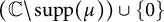 $(\mathbb C\setminus \operatorname {supp}(\mu ))\cup \{0\}$
with
$(\mathbb C\setminus \operatorname {supp}(\mu ))\cup \{0\}$
with
 $f_\alpha (0)=0$
.
$f_\alpha (0)=0$
.
Proof Assume 0 is in
 $\operatorname {supp}(\mu )$
but
$\operatorname {supp}(\mu )$
but
 $(0, c)$
is outside
$(0, c)$
is outside
 $\operatorname {supp}(\mu )$
for some
$\operatorname {supp}(\mu )$
for some
 $c>0$
. Then, for
$c>0$
. Then, for
 $\lambda \notin \operatorname {supp}(\mu )$
, we have
$\lambda \notin \operatorname {supp}(\mu )$
, we have
 $$\begin{align*}\int_0^\infty \frac{\xi+\lambda}{\xi-\lambda}\,d\mu(\xi)=-\mu(\{0\})+\int_c^\infty \frac{\xi+\lambda}{\xi-\lambda}\,d\mu(\xi) \end{align*}$$
and the result follows easily.
Recall from Corollary 3.12 that
 $\operatorname {supp}(\mu )\setminus \{0\}$
is contained in
$\operatorname {supp}(\mu )\setminus \{0\}$
is contained in
 $\overline \Sigma _s$
. Thus, by Lemma 4.1, we can always define
$\overline \Sigma _s$
. Thus, by Lemma 4.1, we can always define
 $f_\alpha $
as a holomorphic function on the complement of
$f_\alpha $
as a holomorphic function on the complement of
 $\overline \Sigma _s$
, even in the case where
$\overline \Sigma _s$
, even in the case where
 $0$
is outside
$0$
is outside
 $\overline \Sigma _s$
and
$\overline \Sigma _s$
and
 $\mu $
has mass at 0.
$\mu $
has mass at 0.
Definition 4.2 For
 $s>0$
and
$s>0$
and
 $\tau \in \mathbb {C}$
such that
$\tau \in \mathbb {C}$
such that
 $|s-\tau | \leq s$
, define a closed set
$|s-\tau | \leq s$
, define a closed set
 $D_{s,\tau }$
by the relation
$D_{s,\tau }$
by the relation
 $$\begin{align*}(D_{s,\tau})^c = f_{s-\tau}((\overline{\Sigma}_s)^c)\end{align*}$$
and
 $$\begin{align*}\Sigma_{s,\tau} = \operatorname{int}(D_{s,\tau}), \end{align*}$$
where we recall from Section 3 that
 $$\begin{align*}\Sigma_s = \{\lambda : \lambda\neq 0 \text{ and } T(\lambda)<s\}.\end{align*}$$
See Figure 2 for examples of the domains
 $D_{s,\tau }$
.
$D_{s,\tau }$
.
We now define the regularized log potential of the Brown measure of
 $xb_{s,\tau }$
, as follows.
$xb_{s,\tau }$
, as follows.
Definition 4.3 Define a function S by
 $$ \begin{align*}S(s,\tau,\lambda,\varepsilon) = \operatorname{tr}\left[\log\left((xb_{s,\tau}-\lambda)^\ast(xb_{s,\tau}-\lambda)+\varepsilon^2\right)\right]\end{align*} $$
for all
 $s>0, \tau \in \mathbb {C}$
with
$s>0, \tau \in \mathbb {C}$
with
 $|\tau -s | \leq s, \lambda \in \mathbb {C},$
and
$|\tau -s | \leq s, \lambda \in \mathbb {C},$
and
 $\varepsilon>0$
.
$\varepsilon>0$
.
Note that while in Section 3, we regularized the log potential of the Brown measure of
 $xb_t$
using
$xb_t$
using
 $\varepsilon $
, as in [Reference Driver, Hall and Kemp10, Reference Ho and Zhong21], here we regularize using
$\varepsilon $
, as in [Reference Driver, Hall and Kemp10, Reference Ho and Zhong21], here we regularize using
 $\varepsilon ^2$
to be consistent with [Reference Hall and Ho17]. This convention will allow us to use formulas from [Reference Hall and Ho17] without change.
$\varepsilon ^2$
to be consistent with [Reference Hall and Ho17]. This convention will allow us to use formulas from [Reference Hall and Ho17] without change.
We now state the main result of this section, whose proof will occupy the rest of the section.
Theorem 4.2 Fix
 $s>0$
and
$s>0$
and
 $\tau \in \mathbb {C}$
such that
$\tau \in \mathbb {C}$
such that
 $|\tau -s|\leq s$
. Then, the following results hold:
$|\tau -s|\leq s$
. Then, the following results hold:
-
(1) The map
$f_{s-\tau }$
is a bijection from
$(\overline {\Sigma }_s)^c$
to
$(D_{s,\tau })^c$
and
$f_{s-\tau }(\lambda )$
tends to infinity as
$\lambda $
tends to infinity. -
(2) For all
$\lambda $
outside of
$D_{s,\tau }$
, we have (4.1)
$$ \begin{align} \frac{\partial S}{\partial \lambda} = \frac{f^{-1}_{s-\tau}(\lambda)}{\lambda}\int_0^{\infty} \frac{1}{f^{-1}_{s-\tau}(\lambda) -\xi} \,d\mu(\xi). \end{align} $$
-
(3) The Brown measure
$\mu _{s,\tau }$
of
$xb_{s,\tau }$
is zero outside
$D_{s,\tau }$
except possibly at the origin. -
(4) If 0 is not in
$D_{s,\tau }$
, we have
$$\begin{align*}\mu_{s,\tau}(\{0\}) = \mu(\{0\}).\end{align*}$$


Note that
 $f_{s-\tau }$
is surjective by Definition 4.2. The right-hand side of
$f_{s-\tau }$
is surjective by Definition 4.2. The right-hand side of
 $(4.1)$
is well-defined since the nonzero closed support of
$(4.1)$
is well-defined since the nonzero closed support of
 $\mu $
lies inside
$\mu $
lies inside
 $\overline {\Sigma }_s$
by Corollary 3.12. This equation also implies that
$\overline {\Sigma }_s$
by Corollary 3.12. This equation also implies that
 $\frac {\partial S}{\partial \lambda }$
is a holomorphic function outside
$\frac {\partial S}{\partial \lambda }$
is a holomorphic function outside
 $D_{s,\tau }$
except possibly at the origin. Therefore,
$D_{s,\tau }$
except possibly at the origin. Therefore,
 $(3)$
follows from
$(3)$
follows from
 $(2)$
.
$(2)$
.
4.2 The PDE method
To obtain Theorem 4.2, we need the following PDE and its Hamiltonian, obtained as Theorem 4.2 in [Reference Hall and Ho17].
Theorem 4.3 (Hall–Ho)
The function S in Definition 4.3 satisfies the PDE
 $$ \begin{align} \frac{\partial S}{\partial \tau} = \frac{1}{8}\left[1-\left(1-\varepsilon \frac{\partial S}{\partial \varepsilon}-2\lambda \frac{\partial S}{\partial \lambda}\right)^2\right] \end{align} $$
for all
 $\lambda \in \mathbb {C}, \tau \in \mathbb {C}$
satisfying
$\lambda \in \mathbb {C}, \tau \in \mathbb {C}$
satisfying
 $|\tau -s| < s,$
and
$|\tau -s| < s,$
and
 $\varepsilon>0$
where
$\varepsilon>0$
where
 $$\begin{align*}\frac{\partial}{\partial \tau} = \frac{1}{2}\left(\frac{\partial}{\partial \tau_1} - i\frac{\partial}{\partial \tau_2}\right) \quad \text{and } \quad \frac{\partial}{\partial \lambda}=\frac{1}{2}\left(\frac{\partial}{\partial \lambda_1} - i\frac{\partial}{\partial \lambda_2}\right)\end{align*}$$
are the Cauchy–Riemann operators and the initial condition at
 $\tau =s$
is given by
$\tau =s$
is given by
 $$ \begin{align*}S(s,s,\lambda,\varepsilon) = \operatorname{tr}\left[\log\left((xb_{s,s}-\lambda)^\ast(xb_{s,s}-\lambda)+\varepsilon^2\right)\right],\end{align*} $$
where
 $b_{s,s}=b_s$
is the free multiplicative Brownian motion considered in Section 3.
$b_{s,s}=b_s$
is the free multiplicative Brownian motion considered in Section 3.
Moreover, from Section 3, in the initial case
 $\tau =s,$
we have that for
$\tau =s,$
we have that for
 $\lambda _0 \notin \overline {\Sigma }_s$
,
$\lambda _0 \notin \overline {\Sigma }_s$
,
 $$ \begin{align} s(s,s,\lambda_0) := \lim_{\varepsilon \rightarrow 0^+} S(s,s,\lambda_0,0) = \int_0^{\infty} \log\left(|\xi-\lambda_0|^2\right)\,d\mu(\xi), \end{align} $$
where
 $\mu $
is the law of the element x.
$\mu $
is the law of the element x.
We now introduce the complex-valued Hamiltonian function, obtained from the PDE (4.2) by replacing each derivative with a momentum variable, with an overall minus sign:
 $$ \begin{align*}H(\lambda,\varepsilon,p_\lambda,p_\varepsilon) = -\frac{1}{8}\left[1-\left(1-\varepsilon p_\varepsilon -2\lambda p_\lambda\right)^2\right].\end{align*} $$
Here, the variables
 $\lambda $
and
$\lambda $
and
 $p_\lambda $
are complex-valued and
$p_\lambda $
are complex-valued and
 $\varepsilon $
and
$\varepsilon $
and
 $p_\varepsilon $
are real-valued. For arbitrary
$p_\varepsilon $
are real-valued. For arbitrary
 $\lambda _0\in \mathbb C$
and
$\lambda _0\in \mathbb C$
and
 $\varepsilon _0>0$
, define initial momenta
$\varepsilon _0>0$
, define initial momenta
 $p_{\lambda ,0}$
and
$p_{\lambda ,0}$
and
 $p_{\varepsilon ,0}$
by
$p_{\varepsilon ,0}$
by
 $$ \begin{align} p_{\lambda,0} = \frac{\partial}{\partial \lambda}S(s,s,\lambda_0,\varepsilon_0) \end{align} $$
 $$ \begin{align} p_{\varepsilon,0} = \frac{\partial}{\partial \varepsilon}S(s,s,\lambda_0,\varepsilon_0). \end{align} $$
We now introduce curves
 $\lambda (\tau )$
,
$\lambda (\tau )$
,
 $\varepsilon (\tau )$
,
$\varepsilon (\tau )$
,
 $p_\lambda (\tau )$
, and
$p_\lambda (\tau )$
, and
 $p_\varepsilon (\tau )$
as in Section 5 in [Reference Hall and Ho17] but with
$p_\varepsilon (\tau )$
as in Section 5 in [Reference Hall and Ho17] but with
 $\tau $
there replaced by
$\tau $
there replaced by
 $\tau -s$
here, since our initial condition is at
$\tau -s$
here, since our initial condition is at
 $\tau =s$
:
$\tau =s$
:
 $$ \begin{align} \lambda(\tau) &= \lambda_0\exp\left\{\frac{\tau-s}{2}\left(\varepsilon_0p_{\varepsilon,0} + 2\lambda_0p_{\lambda,0} - 1\right)\right\} \end{align} $$
 $$ \begin{align} \varepsilon(\tau) &= \varepsilon_0\exp\left\{\Re\left[\frac{\tau-s}{2}\left(\varepsilon_0p_{\varepsilon,0} + 2\lambda_0p_{\lambda,0} - 1\right)\right]\right\} \end{align} $$
 $$ \begin{align} p_\lambda(\tau) &= p_{\lambda,0}\exp\left\{-\frac{\tau-s}{2}\left(\varepsilon_0p_{\varepsilon,0} + 2\lambda_0p_{\lambda,0} - 1\right)\right\} \end{align} $$
 $$ \begin{align} p_{\varepsilon}(\tau) &=p_{\varepsilon,0}\exp\left\{-\Re\left[\frac{\tau-s}{2}\left(\varepsilon_0p_{\varepsilon,0} + 2\lambda_0p_{\lambda,0} - 1\right)\right] \right\}. \end{align} $$
The initial values in all cases denote the values of the curves at
 $\tau =s$
; for example,
$\tau =s$
; for example,
 $\lambda _0$
is the value of
$\lambda _0$
is the value of
 $\lambda (\tau )$
at
$\lambda (\tau )$
at
 $\tau =s$
.
$\tau =s$
.
Hall and Ho develop [Reference Hall and Ho17, Section 4] Hamilton–Jacobi formulas for solutions to the PDE (4.2) by reducing the equations to an ordinary Hamilton–Jacobi PDE with a real time variable. These formulas hold initially for
 $\vert \tau -s\vert <s$
but extend by continuity to the boundary case
$\vert \tau -s\vert <s$
but extend by continuity to the boundary case
 $|s-\tau | = s$
, as in [Reference Hall and Ho17, Proposition 5.5]. We therefore obtain the following result.
$|s-\tau | = s$
, as in [Reference Hall and Ho17, Proposition 5.5]. We therefore obtain the following result.
Theorem 4.4 (Hall–Ho)
For all
 $\tau $
with
$\tau $
with
 $|\tau -s| \leq s,$
we have the first Hamilton–Jacobi formula
$|\tau -s| \leq s,$
we have the first Hamilton–Jacobi formula
 $$ \begin{align} \begin{aligned} S(s,\tau,\lambda(\tau),\varepsilon(\tau)) &= S(s,s,\lambda_0,\varepsilon_0) + 2 \Re[(\tau-s) H_0] \\&\quad+\frac{1}{2}\Re\left[(\tau-s)(\varepsilon_0p_{\varepsilon,0}+2\lambda_0p_{\lambda,0})\right], \end{aligned} \end{align} $$
where
 $H_0 = H(\lambda _0,\varepsilon _0,p_{\lambda ,0},p_{\varepsilon ,0}),$
and the second Hamilton–Jacobi formulas
$H_0 = H(\lambda _0,\varepsilon _0,p_{\lambda ,0},p_{\varepsilon ,0}),$
and the second Hamilton–Jacobi formulas
 $$ \begin{align} \frac{\partial S}{\partial \lambda}(s,\tau,\lambda(\tau),\varepsilon(\tau)) &= p_\lambda(\tau) \end{align} $$
 $$ \begin{align} \frac{\partial S}{\partial \varepsilon}(s,\tau,\lambda(\tau),\varepsilon(\tau)) &= p_\varepsilon(\tau). \end{align} $$
4.3 The
$\varepsilon \rightarrow 0$
limit

We are then interested in the behavior of the curves in (4.6)–(4.9) in the limit as
 $\varepsilon $
tends to zero.
$\varepsilon $
tends to zero.
Lemma 4.5 Suppose that
 $\lambda _0$
is a nonzero point outside
$\lambda _0$
is a nonzero point outside
 $\overline \Sigma _s$
. Then, for all
$\overline \Sigma _s$
. Then, for all
 $\tau $
with
$\tau $
with
 $|\tau -s| \leq s,$
the limits as
$|\tau -s| \leq s,$
the limits as
 $\varepsilon _0\rightarrow 0$
of
$\varepsilon _0\rightarrow 0$
of
 $p_{\varepsilon ,0}$
and
$p_{\varepsilon ,0}$
and
 $\lambda _0p_{\lambda ,0}$
exist and
$\lambda _0p_{\lambda ,0}$
exist and
 $$\begin{align*}\lim_{\varepsilon_0 \rightarrow 0}\lambda(\tau) = f_{s-\tau}(\lambda_0).\end{align*}$$
The same result holds for
 $\lambda _0=0$
, provided that
$\lambda _0=0$
, provided that
 $0\notin \overline \Sigma _s$
and
$0\notin \overline \Sigma _s$
and
 $0\notin \operatorname {supp}(\mu )$
.
$0\notin \operatorname {supp}(\mu )$
.
Proof Let
 $\lambda _0 \notin \overline {\Sigma }_s$
be nonzero. Then,
$\lambda _0 \notin \overline {\Sigma }_s$
be nonzero. Then,
 $p_{\varepsilon ,0}$
is the same as
$p_{\varepsilon ,0}$
is the same as
 $p_0$
in (3.10) in Section 3. Thus, by Corollary 3.12,
$p_0$
in (3.10) in Section 3. Thus, by Corollary 3.12,
 $p_{\varepsilon ,0}$
remains finite as
$p_{\varepsilon ,0}$
remains finite as
 $\varepsilon _0 \rightarrow 0$
. Meanwhile, as
$\varepsilon _0 \rightarrow 0$
. Meanwhile, as
 $\varepsilon _0 \rightarrow 0$
, we have
$\varepsilon _0 \rightarrow 0$
, we have
 $$ \begin{align*} p_{\lambda,0} &= \frac{\partial}{\partial \lambda_0} S(s,s,\lambda_0,\varepsilon_0)\\ &= \frac{\partial}{\partial \lambda_0} \int_0^{\infty} \log\left(|\xi-\lambda_0|^2\right)d\mu(\xi) \\ &= \int_0^{\infty} \frac{1}{\lambda_0 -\xi} \,d\mu(\xi). \end{align*} $$
It follows that
 $$ \begin{align*} \lim_{\varepsilon_0 \rightarrow 0} 2\lambda_0p_{\lambda,0} -1 &= 2\lambda_0 \int_0^{\infty} \frac{1}{\lambda_0 -\xi} \,d\mu(\xi) -1\\ &= - \int_0^{\infty} \frac{\xi+\lambda_0}{\xi-\lambda_0} \,d\mu(\xi). \end{align*} $$
Hence, letting
 $\varepsilon $
tend to zero in the formula
$\varepsilon $
tend to zero in the formula
 $({4.6})$
for
$({4.6})$
for
 $\lambda (\tau )$
, we get
$\lambda (\tau )$
, we get
 $$ \begin{align*} \lim_{\varepsilon_0 \rightarrow 0}\lambda(\tau) &= \lim_{\varepsilon_0 \rightarrow 0} \lambda_0\exp\left\{\frac{\tau-s}{2}\left(\varepsilon_0p_{\varepsilon,0} + 2\lambda_0p_{\lambda,0} - 1\right)\right\}\\ &= \lambda_0\exp\left[\frac{\tau-s}{2}\left(-\int_0^{\infty} \frac{\xi+\lambda_0}{\xi-\lambda_0} \,d\mu(\xi)\right)\right] \\ &= f_{s-\tau}(\lambda_0). \end{align*} $$
The same calculation is applicable if
 $\lambda _0\notin \overline \Sigma _s$
equals 0, provided that 0 is not in the support of
$\lambda _0\notin \overline \Sigma _s$
equals 0, provided that 0 is not in the support of
 $\mu $
.
$\mu $
.
Proposition 4.6 Define the map
 $\phi _\tau $
from
$\phi _\tau $
from
 $\mathbb {C} \times (0, \infty )$
into
$\mathbb {C} \times (0, \infty )$
into
 $\mathbb {C}\times (0, \infty )$
by
$\mathbb {C}\times (0, \infty )$
by
 $$ \begin{align*}\phi_\tau(\lambda_0,\varepsilon_0) = (\lambda(\tau),\varepsilon(\tau)),\end{align*} $$
where
 $\lambda (\tau )$
and
$\lambda (\tau )$
and
 $\varepsilon (\tau )$
are computed with
$\varepsilon (\tau )$
are computed with
 $\lambda (s) = \lambda _0$
and
$\lambda (s) = \lambda _0$
and
 $\varepsilon (s) = \varepsilon _0$
and the initial momenta
$\varepsilon (s) = \varepsilon _0$
and the initial momenta
 $p_{\lambda ,0}$
and
$p_{\lambda ,0}$
and
 $p_{\varepsilon ,0}$
given by (4.4) and (4.5). Then, for all nonzero
$p_{\varepsilon ,0}$
given by (4.4) and (4.5). Then, for all nonzero
 $\lambda _0 \in (\overline {\Sigma }_s)^c$
, the map
$\lambda _0 \in (\overline {\Sigma }_s)^c$
, the map
 $\phi _\tau $
extends analytically to a neighborhood of
$\phi _\tau $
extends analytically to a neighborhood of
 $\varepsilon _0 =0$
as a map into
$\varepsilon _0 =0$
as a map into
 $\mathbb C\times \mathbb R$
. Moreover, Jacobian of
$\mathbb C\times \mathbb R$
. Moreover, Jacobian of
 $\phi _\tau $
at
$\phi _\tau $
at
 $(\lambda _0,0$
) is invertible if and only if
$(\lambda _0,0$
) is invertible if and only if
 $f^{\prime }_{s-\tau }(\lambda _0) \neq 0$
.
$f^{\prime }_{s-\tau }(\lambda _0) \neq 0$
.
Proof By Corollary 3.12, every nonzero
 $\lambda _0$
in
$\lambda _0$
in
 $(\overline {\Sigma }_s)^c$
is outside of the closed support of
$(\overline {\Sigma }_s)^c$
is outside of the closed support of
 $\mu $
. Then, the formulas
$\mu $
. Then, the formulas
 $({4.4})$
and
$({4.4})$
and
 $({4.5})$
for the initial momenta
$({4.5})$
for the initial momenta
 $p_{\lambda ,0}$
and
$p_{\lambda ,0}$
and
 $p_{\varepsilon ,0}$
are well defined and analytic even in a neighborhood of
$p_{\varepsilon ,0}$
are well defined and analytic even in a neighborhood of
 $\varepsilon _0 =0$
. Thus, the formulas
$\varepsilon _0 =0$
. Thus, the formulas
 $({4.6})$
and
$({4.6})$
and
 $({4.7})$
for
$({4.7})$
for
 $\lambda (\tau )$
and
$\lambda (\tau )$
and
 $\varepsilon (\tau )$
depend analytically on
$\varepsilon (\tau )$
depend analytically on
 $\lambda _0$
and
$\lambda _0$
and
 $\varepsilon _0$
.
$\varepsilon _0$
.
Now, to compute the Jacobian of
 $\phi _\tau $
at
$\phi _\tau $
at
 $(\lambda _0,0)$
, we write
$(\lambda _0,0)$
, we write
 $\lambda _0 = x_0 +iy_0.$
Differentiating (4.6) and evaluating at
$\lambda _0 = x_0 +iy_0.$
Differentiating (4.6) and evaluating at
 $\varepsilon _0 =0$
gives
$\varepsilon _0 =0$
gives
 $$ \begin{align*}\frac{\partial \varepsilon}{\partial x_0} = 0;\quad \frac{\partial \varepsilon}{\partial y_0} = 0; \quad\frac{\partial \varepsilon}{\partial \varepsilon_0} = \exp\left(\Re\left[\frac{\tau-s}{2}(2\lambda_0p_{\lambda,0}-1)\right]\right)> 0.\end{align*} $$
Meanwhile, when
 $\varepsilon _0 =0$
, Lemma 4.5 tells us that
$\varepsilon _0 =0$
, Lemma 4.5 tells us that
 $\lambda (\tau ) = f_{s-\tau }(\lambda _0)$
. Thus, Jacobian of
$\lambda (\tau ) = f_{s-\tau }(\lambda _0)$
. Thus, Jacobian of
 $\phi _\tau $
has the form:
$\phi _\tau $
has the form:
 $$ \begin{align*}\begin{pmatrix} J & \ast \\ 0 & \frac{\partial \varepsilon}{\partial \varepsilon_0} \end{pmatrix},\end{align*} $$
where J is the Jacobian of
 $f_{s-\tau }(\lambda _0)$
at
$f_{s-\tau }(\lambda _0)$
at
 $\lambda _0$
(that is, the complex number
$\lambda _0$
(that is, the complex number
 $f_{s-\tau }'(\lambda _0)$
, viewed as a
$f_{s-\tau }'(\lambda _0)$
, viewed as a
 $2\times 2$
matrix). Therefore, the Jacobian of
$2\times 2$
matrix). Therefore, the Jacobian of
 $\phi _\tau $
at
$\phi _\tau $
at
 $(\lambda _0,0)$
is invertible if and only if
$(\lambda _0,0)$
is invertible if and only if
 $f^{\prime }_{s-\tau }(\lambda _0) \neq 0$
.
$f^{\prime }_{s-\tau }(\lambda _0) \neq 0$
.
Proposition 4.7 Fix
 $\tau $
with
$\tau $
with
 $|\tau -s| \leq s$
and a nonzero point
$|\tau -s| \leq s$
and a nonzero point
 $w \in (D_{s,\tau })^c$
. Choose
$w \in (D_{s,\tau })^c$
. Choose
 $w_0 \in (\overline {\Sigma }_s)^c$
such that
$w_0 \in (\overline {\Sigma }_s)^c$
such that
 $f_{s-\tau }(w_0) = w$
, where such a
$f_{s-\tau }(w_0) = w$
, where such a
 $w_0$
exists by Definition 4.2. If
$w_0$
exists by Definition 4.2. If
 $f^{\prime }_{s-\tau }(w_0) \neq 0$
, then the map
$f^{\prime }_{s-\tau }(w_0) \neq 0$
, then the map
 $$ \begin{align*}(\lambda,\varepsilon) \mapsto S(s,\tau,\lambda,\varepsilon),\end{align*} $$
initially defined for
 $\varepsilon>0$
, has an analytic extension defined for
$\varepsilon>0$
, has an analytic extension defined for
 $(\lambda ,\varepsilon )$
in a neighborhood of
$(\lambda ,\varepsilon )$
in a neighborhood of
 $(w,0)$
.
$(w,0)$
.
Proof We let HJ
 $(s,\tau ,\lambda _0,\varepsilon _0)$
denote the right-hand side of the first Hamilton–Jacobi formula (4.10), i.e.,
$(s,\tau ,\lambda _0,\varepsilon _0)$
denote the right-hand side of the first Hamilton–Jacobi formula (4.10), i.e.,
 $$ \begin{align*} \text{HJ}(s,\tau, & \lambda_0,\varepsilon_0) \\ & =S(s,s,\lambda_0,\varepsilon_0) + 2 \Re[(\tau-s) H_0] +\frac{1}{2}\Re\left[(\tau-s)(\varepsilon_0p_{\varepsilon,0}+2\lambda_0p_{\lambda,0})\right]. \end{align*} $$
Fix a nonzero
 $w \in (D_{s,\tau })^c$
and pick
$w \in (D_{s,\tau })^c$
and pick
 $w_0 \in (\overline {\Sigma }_s)^c$
such that
$w_0 \in (\overline {\Sigma }_s)^c$
such that
 $f_{s-\tau }(w_0) =w$
. By Lemma 4.5 with
$f_{s-\tau }(w_0) =w$
. By Lemma 4.5 with
 $\varepsilon _0 =0$
, we have
$\varepsilon _0 =0$
, we have
 $\lambda (\tau )= f_{s-\tau }(w_0) =w$
. By Proposition 4.6, the map
$\lambda (\tau )= f_{s-\tau }(w_0) =w$
. By Proposition 4.6, the map
 $\phi _\tau $
has a local inverse near
$\phi _\tau $
has a local inverse near
 $(w_0,0)$
, provided that
$(w_0,0)$
, provided that
 $f_{s-\tau }'(w_0)\neq 0$
.
$f_{s-\tau }'(w_0)\neq 0$
.
We may therefore define a function
 $\tilde S$
by
$\tilde S$
by
 $$ \begin{align*}\tilde{S}(s,\tau,\lambda,\varepsilon) = \text{HJ}(s,\tau,\phi_\tau^{-1}(\lambda,\varepsilon)).\end{align*} $$
Then,
 $\tilde {S}$
agrees with S as long as the first Hamilton–Jacobi formula (4.10) is applicable, namely, for
$\tilde {S}$
agrees with S as long as the first Hamilton–Jacobi formula (4.10) is applicable, namely, for
 $\varepsilon _0>0$
. Thus,
$\varepsilon _0>0$
. Thus,
 $\tilde {S}$
will be the desired analytic extension, provided that
$\tilde {S}$
will be the desired analytic extension, provided that
 $f^{\prime }_{s-\tau }(w_0) \neq 0$
.
$f^{\prime }_{s-\tau }(w_0) \neq 0$
.
We now want to let
 $\varepsilon _0$
tend to zero in the second Hamilton–Jacobi formula (4.11). We do this at first for points
$\varepsilon _0$
tend to zero in the second Hamilton–Jacobi formula (4.11). We do this at first for points
 $\lambda $
outside
$\lambda $
outside
 $D_{s,\tau }$
for which we can find
$D_{s,\tau }$
for which we can find
 $\lambda _0$
outside
$\lambda _0$
outside
 $\overline \Sigma _s$
with
$\overline \Sigma _s$
with
 $f_{s-\tau }(\lambda _0)=\lambda $
and
$f_{s-\tau }(\lambda _0)=\lambda $
and
 $f_{s-\tau }'(\lambda _0)\neq 0$
.
$f_{s-\tau }'(\lambda _0)\neq 0$
.
Proposition 4.8 Fix
 $\tau $
with
$\tau $
with
 $|\tau -s| \leq s$
and a nonzero point
$|\tau -s| \leq s$
and a nonzero point
 $\lambda \in (D_{s,\tau })^c$
. Choose
$\lambda \in (D_{s,\tau })^c$
. Choose
 $\lambda _0 \in (\overline {\Sigma }_s)^c$
such that
$\lambda _0 \in (\overline {\Sigma }_s)^c$
such that
 $f_{s-\tau }(\lambda _0) = \lambda $
, and assume that
$f_{s-\tau }(\lambda _0) = \lambda $
, and assume that
 $f^{\prime }_{s-\tau }(\lambda _0) \neq 0$
. Then, the analytic extension of S given by Proposition 4.7 satisfies
$f^{\prime }_{s-\tau }(\lambda _0) \neq 0$
. Then, the analytic extension of S given by Proposition 4.7 satisfies
 $$ \begin{align} \frac{\partial S}{\partial \lambda}(s,\tau,\lambda,0) = \frac{f^{-1}_{s-\tau}(\lambda)}{\lambda}\int_0^{\infty} \frac{1}{f^{-1}_{s-\tau}(\lambda) -\xi} \,d\mu(\xi), \end{align} $$
where the inverse is taken locally.
Proof Since
 $f^{\prime }_{s-\tau }(\lambda _0)\neq 0$
, it directly follows from Proposition 4.7 that we can let
$f^{\prime }_{s-\tau }(\lambda _0)\neq 0$
, it directly follows from Proposition 4.7 that we can let
 $\varepsilon _0 \rightarrow 0$
in the second Hamilton–Jacobi formula
$\varepsilon _0 \rightarrow 0$
in the second Hamilton–Jacobi formula
 $({4.11})$
. Now, if we compare the formulas (4.6) and (4.8), we see that
$({4.11})$
. Now, if we compare the formulas (4.6) and (4.8), we see that
 $$\begin{align*}p_\lambda(\tau)=p_{\lambda,0}\frac{\lambda_0}{\lambda(\tau)}. \end{align*}$$
Furthermore, by Lemma 4.5, we have (with
 $\varepsilon =0$
) that
$\varepsilon =0$
) that
 $\lambda (\tau )= f_{s-\tau }(\lambda _0)=\lambda $
. Thus, the analytic extension of S satisfies
$\lambda (\tau )= f_{s-\tau }(\lambda _0)=\lambda $
. Thus, the analytic extension of S satisfies
 $$ \begin{align*} \frac{\partial S}{\partial \lambda}(s,\tau,\lambda,0) &= \frac{\lambda_0}{\lambda}p_{\lambda,0}\\ &= \frac{\lambda_0}{f_{s-\tau}(\lambda_0)}\int_0^{\infty} \frac{1}{\lambda_0 -\xi} \,d\mu(\xi) \\ &= \frac{f^{-1}_{s-\tau}(\lambda)}{\lambda}\int_0^{\infty} \frac{1}{f^{-1}_{s-\tau}(\lambda) -\xi} \,d\mu(\xi), \end{align*} $$
where the inverse is locally defined and holomorphic by the holomorphic version of the inverse function theorem.
Proposition 4.9 The Brown measure of
 $xb_{s,\tau }$
is zero outside
$xb_{s,\tau }$
is zero outside
 $D_{s,\tau }$
, except possibly at the origin.
$D_{s,\tau }$
, except possibly at the origin.
Proof For all nonzero
 $w\in (D_{s,\tau })^c$
, Proposition 4.8 exhibits
$w\in (D_{s,\tau })^c$
, Proposition 4.8 exhibits
 $\partial S/\partial \lambda (s,\tau ,\lambda ,0)$
near w as a holomorphic function, provided that there is
$\partial S/\partial \lambda (s,\tau ,\lambda ,0)$
near w as a holomorphic function, provided that there is
 $\lambda _0\notin \overline \Sigma _s$
with
$\lambda _0\notin \overline \Sigma _s$
with
 $f_{s-\tau }(\lambda _0)=\lambda $
and
$f_{s-\tau }(\lambda _0)=\lambda $
and
 $f_{s-\tau }'(\lambda _0)\neq 0$
. Then, the Brown measure of
$f_{s-\tau }'(\lambda _0)\neq 0$
. Then, the Brown measure of
 $xb_{s,\tau }$
, obtained by taking a
$xb_{s,\tau }$
, obtained by taking a
 $\bar \lambda $
derivative, is therefore zero near any such
$\bar \lambda $
derivative, is therefore zero near any such
 $\lambda $
.
$\lambda $
.
Now suppose that
 $\lambda \neq 0$
is outside
$\lambda \neq 0$
is outside
 $D_{s,\tau }$
and that for all
$D_{s,\tau }$
and that for all
 $\lambda _0\notin \overline \Sigma _s$
such that
$\lambda _0\notin \overline \Sigma _s$
such that
 $f_{s,\tau }(\lambda _0)=\lambda $
, we have
$f_{s,\tau }(\lambda _0)=\lambda $
, we have
 $f_{s,\tau }'(\lambda _0)=0$
. Then, any one such
$f_{s,\tau }'(\lambda _0)=0$
. Then, any one such
 $\lambda _0$
will be an isolated zero of
$\lambda _0$
will be an isolated zero of
 $f_{s,\tau }$
. By the open mapping theorem and the result in the previous paragraph, the Brown measure of
$f_{s,\tau }$
. By the open mapping theorem and the result in the previous paragraph, the Brown measure of
 $xb_{s,\tau }$
will be zero in a punctured neighborhood of
$xb_{s,\tau }$
will be zero in a punctured neighborhood of
 $\lambda $
. If the Brown measure assigned positive mass to
$\lambda $
. If the Brown measure assigned positive mass to
 ${\lambda }$
(but is zero in a punctured neighborhood of
${\lambda }$
(but is zero in a punctured neighborhood of
 $\lambda $
), then
$\lambda $
), then
 $S(s,\tau ,\lambda ,0)$
would have a logarithmic singularity at
$S(s,\tau ,\lambda ,0)$
would have a logarithmic singularity at
 $\lambda $
and
$\lambda $
and
 $\partial S/\partial \lambda (s,\tau ,\lambda ,0)$
would blow up at
$\partial S/\partial \lambda (s,\tau ,\lambda ,0)$
would blow up at
 $\lambda $
. But if we evaluate
$\lambda $
. But if we evaluate
 $({4.13})$
at w and let w tend to
$({4.13})$
at w and let w tend to
 $\lambda $
, we get
$\lambda $
, we get
 $$ \begin{align*} \lim_{w \rightarrow \lambda} \frac{\partial }{\partial \lambda}S(s,\tau,w,0) = \lim_{w_0 \rightarrow \lambda_0}\frac{w_0}{f_{s-\tau}(w_0)}\int_0^{\infty} \frac{1}{w_0 -\xi} \,d\mu(\xi), \end{align*} $$
which remains bounded.
Proposition 4.10 If
 $0$
is not in
$0$
is not in
 $D_{s,\tau }$
, the Brown measure
$D_{s,\tau }$
, the Brown measure
 $\mu _{s,\tau }$
of
$\mu _{s,\tau }$
of
 $xb_{s,\tau }$
satisfies
$xb_{s,\tau }$
satisfies
 $$\begin{align*}\mu_{s,\tau}(\{0\}) = \mu(\{0\}).\end{align*}$$
Proof Note that since
 $f_{s-\tau }(\lambda _0)$
has a simple zero at
$f_{s-\tau }(\lambda _0)$
has a simple zero at
 $\lambda _0 =0$
, we can construct a local inverse
$\lambda _0 =0$
, we can construct a local inverse
 $f_{s,\tau }^{-1}$
near 0 having a simple zero at 0. Then,
$f_{s,\tau }^{-1}$
near 0 having a simple zero at 0. Then,
 $f^{-1}_{s-\tau }(\lambda )/\lambda $
has a removable zero at
$f^{-1}_{s-\tau }(\lambda )/\lambda $
has a removable zero at
 $\lambda =0$
. Also, recall from Corollary 3.12 that if 0 is outside
$\lambda =0$
. Also, recall from Corollary 3.12 that if 0 is outside
 $\overline \Sigma _s$
, it is an isolated point in
$\overline \Sigma _s$
, it is an isolated point in
 $\operatorname {supp}(\mu )$
. In that case, we can find
$\operatorname {supp}(\mu )$
. In that case, we can find
 $c>0$
such that
$c>0$
such that
 $(0, c) \cap \operatorname {supp}(\mu ) = \varnothing $
and (4.13) becomes
$(0, c) \cap \operatorname {supp}(\mu ) = \varnothing $
and (4.13) becomes
 $$ \begin{align} \frac{\partial S}{\partial \lambda}(s,\tau,\lambda,0) = \frac{\mu(\{0\})}{\lambda} + \frac{f^{-1}_{s-\tau}(\lambda)}{\lambda}\int_c^\infty \frac{1}{f^{-1}_{s-\tau}(\lambda) -\xi} \,d\mu(\xi). \end{align} $$
Since the second term on the right-hand side of (4.14) is holomorphic near the origin, we can take the distributional
 $\lambda $
-bar derivative to obtain the distributional Laplacian, giving
$\lambda $
-bar derivative to obtain the distributional Laplacian, giving
 $$\begin{align*}\mu_{s,\tau}(\{0\})= \mu(\{0\}) \end{align*}$$
as claimed.
Proposition 4.11 For all s and
 $\tau $
with
$\tau $
with
 $\vert s-\tau \vert \leq s$
, the following results hold:
$\vert s-\tau \vert \leq s$
, the following results hold:
-
(1) The function
$f_{s-\tau }$
is injective on the complement of
$\overline \Sigma _s$
. -
(2) The quantity
$f_{s-\tau }(\lambda _0)$
tends to infinity as
$\lambda _0$
tends to infinity. -
(3) The set
$D_{s,\tau }$
is compact. -
(4) Assume that
$\vert \tau -s\vert <s$
, that the condition (3.25) in Remark 3.11 holds, and that
$0\notin \partial \Sigma _s$
. Then,
$f_{s-\tau }$
is defined and injective on the complement of
$\Sigma _s$
.


Point 4 of the proposition says that (under the stated assumptions), the injectivity of
 $f_{s-\tau }$
in Point 1 extends to the boundary of
$f_{s-\tau }$
in Point 1 extends to the boundary of
 $\Sigma _s$
. The assumption
$\Sigma _s$
. The assumption
 $\vert \tau -s\vert <s$
in Point 4 cannot be omitted. Consider, for example, the case
$\vert \tau -s\vert <s$
in Point 4 cannot be omitted. Consider, for example, the case
 $\tau =0$
(so that
$\tau =0$
(so that
 $\vert \tau -s\vert =s$
) and
$\vert \tau -s\vert =s$
) and
 $x=1$
. In that case, the map
$x=1$
. In that case, the map
 $f_{s-\tau }=f_s$
has already been studied in [Reference Biane4, Reference Driver, Hall and Kemp10] and maps the boundary of
$f_{s-\tau }=f_s$
has already been studied in [Reference Biane4, Reference Driver, Hall and Kemp10] and maps the boundary of
 $\Sigma _s$
in a generically two-to-one fashion to the unit circle. Specifically, points on the boundary with the same argument but different radii have the same value of
$\Sigma _s$
in a generically two-to-one fashion to the unit circle. Specifically, points on the boundary with the same argument but different radii have the same value of
 $f_s$
. See Figure 7 in Section 5 along with the discussion surrounding Proposition 2.5 in [Reference Driver, Hall and Kemp10].
$f_s$
. See Figure 7 in Section 5 along with the discussion surrounding Proposition 2.5 in [Reference Driver, Hall and Kemp10].

Figure 7: The domains
 $\overline \Sigma _s$
(left) and
$\overline \Sigma _s$
(left) and
 $D_{s,0}$
(right) with
$D_{s,0}$
(right) with
 $s=2$
and
$s=2$
and
 $\mu =\delta _1$
.
$\mu =\delta _1$
.
Proof Now that the Brown measure of
 $xb_{s,\tau }$
is known (Proposition 4.9) to be zero outside
$xb_{s,\tau }$
is known (Proposition 4.9) to be zero outside
 $D_{s,\tau }$
, we know that
$D_{s,\tau }$
, we know that
 $\partial S/\partial \lambda (s,\tau ,\lambda ,0)$
is holomorphic outside
$\partial S/\partial \lambda (s,\tau ,\lambda ,0)$
is holomorphic outside
 $D_{s,\tau }$
. It is then possible to use Proposition 4.8 to show that
$D_{s,\tau }$
. It is then possible to use Proposition 4.8 to show that
 $f_{s,\tau }'$
is nonzero outside
$f_{s,\tau }'$
is nonzero outside
 $D_{s,\tau }$
, showing that
$D_{s,\tau }$
, showing that
 $f_{s,\tau }$
is locally injective. The argument is that if
$f_{s,\tau }$
is locally injective. The argument is that if
 $f_{s,\tau }'(\lambda _0)=0$
, then
$f_{s,\tau }'(\lambda _0)=0$
, then
 $\partial S/\partial \lambda $
would blow up at
$\partial S/\partial \lambda $
would blow up at
 $f_{s,\tau }(\lambda _0)$
. We omit the details because we will prove global injectivity by a different method.
$f_{s,\tau }(\lambda _0)$
. We omit the details because we will prove global injectivity by a different method.
To obtain global injectivity, we use an argument similar to Proposition 5.1 in [Reference Zhong26], by considering the second Hamilton–Jacobi formula (4.11). The argument is briefly as follows. We know from Proposition 4.7 that
 $S(s,\tau ,\lambda ,\varepsilon )$
has an analytic extension to
$S(s,\tau ,\lambda ,\varepsilon )$
has an analytic extension to
 $\varepsilon =0$
, for
$\varepsilon =0$
, for
 $\lambda \in (D_{s,\tau })^c$
. If there were two different initial conditions
$\lambda \in (D_{s,\tau })^c$
. If there were two different initial conditions
 $\lambda _0$
and
$\lambda _0$
and
 $\tilde \lambda _0$
giving the same value of
$\tilde \lambda _0$
giving the same value of
 $f_{s-\tau }$
– and thus, by Lemma 4.5, the same value of
$f_{s-\tau }$
– and thus, by Lemma 4.5, the same value of
 $\lambda (\tau )$
at
$\lambda (\tau )$
at
 $\varepsilon _0=0$
– we would get two different values for
$\varepsilon _0=0$
– we would get two different values for
 $\partial S/\partial \lambda (s,\tau ,\lambda ,0)$
at the same
$\partial S/\partial \lambda (s,\tau ,\lambda ,0)$
at the same
 $\lambda $
.
$\lambda $
.
Filling in the details, we use the notation
 $$ \begin{align*}s(s,\tau,\lambda)=S(s,\tau,\lambda,0).\end{align*} $$
We first note that, in the case
 $0\notin \overline \Sigma _s$
, we have from Definition 4.1 that
$0\notin \overline \Sigma _s$
, we have from Definition 4.1 that
 $f_{s-\tau }(\lambda _0)=0$
if and only if
$f_{s-\tau }(\lambda _0)=0$
if and only if
 $\lambda _0=0$
. Using Proposition 4.7, we can let
$\lambda _0=0$
. Using Proposition 4.7, we can let
 $\varepsilon $
tend to 0 in the second Hamilton–Jacobi formula (4.11). We therefore obtain
$\varepsilon $
tend to 0 in the second Hamilton–Jacobi formula (4.11). We therefore obtain
 $$ \begin{align*} \lambda(\tau)\frac{\partial s}{\partial \lambda}\left(\lambda(\tau),\tau\right)&= \lambda(\tau)p_\lambda(\tau) = \lambda_0 p_{\lambda,0}, \end{align*} $$
where the second equality follows from the explicit formulas (4.6) and (4.8).
Now, if two initial conditions
 $\lambda _0$
and
$\lambda _0$
and
 $\tilde {\lambda }_0$
give the same value of
$\tilde {\lambda }_0$
give the same value of
 $f_{s-\tau } = \lambda (\tau )$
, then
$f_{s-\tau } = \lambda (\tau )$
, then
 $$ \begin{align} \lambda_0p_{\lambda,0} = \lambda(\tau)\frac{\partial s}{\partial \lambda}\left(\lambda(\tau),\tau\right) =\tilde{\lambda_0} \tilde{p}_{\lambda,0}. \end{align} $$
But then by the calculation in the proof of Lemma 4.5, we have
 $$ \begin{align*} \lambda_0\exp\left[\frac{\tau-s}{2}\left(2\lambda_0 p_{\lambda,0}-1\right)\right] &=f_{s-\tau}(\lambda_0) \\ &= f_{s-\tau}(\tilde{\lambda}_0) \\ &= \tilde{\lambda}_0\exp\left[\frac{\tau-s}{2}\left(2\tilde{\lambda}_0 \tilde{p}_{\lambda,0}-1\right)\right]. \end{align*} $$
But since, by (4.15),
 $\lambda _0p_{\lambda ,0}=\tilde \lambda _0\tilde p_{\lambda ,0}$
, we must have
$\lambda _0p_{\lambda ,0}=\tilde \lambda _0\tilde p_{\lambda ,0}$
, we must have
 $\lambda _0=\tilde \lambda _0$
.
$\lambda _0=\tilde \lambda _0$
.
Next, we have that
 $$\begin{align*}\lim_{\lambda_0\rightarrow \infty} \int_0^{\infty} \frac{\xi+\lambda_0}{\xi-\lambda_0} \,d\mu(\xi) = -1.\end{align*}$$
That is,
 $$ \begin{align*} \lim_{\lambda_0\rightarrow \infty} f_{s-\tau}(\lambda_0) = \lim_{\lambda_0\rightarrow \infty} \lambda_0 \exp\left[\frac{\tau-s}{2}\right] = \infty, \end{align*} $$
as claimed.
Thus,
 $f_{s-\tau }$
extends to a holomorphic function on a neighborhood of
$f_{s-\tau }$
extends to a holomorphic function on a neighborhood of
 $\infty $
on the Riemann sphere, mapping
$\infty $
on the Riemann sphere, mapping
 $\infty $
to
$\infty $
to
 $\infty $
. Then, by the open mapping theorem, the image of
$\infty $
. Then, by the open mapping theorem, the image of
 $f_{s-\tau }$
contains a neighborhood of
$f_{s-\tau }$
contains a neighborhood of
 $\infty $
. Since, also,
$\infty $
. Since, also,
 $\Sigma _s$
is bounded by Point 3 of Proposition 3.10, we see that
$\Sigma _s$
is bounded by Point 3 of Proposition 3.10, we see that
 $D_{s,\tau }$
(as defined in Definition 4.2) is a closed and bounded (i.e., compact) set.
$D_{s,\tau }$
(as defined in Definition 4.2) is a closed and bounded (i.e., compact) set.
We now address the last point in the proposition. If the condition (3.25) holds, then by Remark 3.11,
 $T\equiv 0$
on
$T\equiv 0$
on
 $\operatorname {supp}(\mu )\setminus \{0\}$
, so that
$\operatorname {supp}(\mu )\setminus \{0\}$
, so that
 $\operatorname {supp}(\mu )\setminus \{0\}$
is contained in
$\operatorname {supp}(\mu )\setminus \{0\}$
is contained in
 $\Sigma _r$
for all
$\Sigma _r$
for all
 $r>0$
. Thus, by Lemma 4.1, the domain of definition of
$r>0$
. Thus, by Lemma 4.1, the domain of definition of
 $f_{s-\tau }$
contains the complement of
$f_{s-\tau }$
contains the complement of
 $\Sigma _s$
. Now, since
$\Sigma _s$
. Now, since
 $\vert \tau -s\vert <s$
, we have
$\vert \tau -s\vert <s$
, we have
 $$\begin{align*}\vert(\tau-\varepsilon)-(s-\varepsilon)\vert=\vert\tau-s\vert<s-\varepsilon \end{align*}$$
for sufficiently small
 $\varepsilon $
. Thus, we can apply Point 1 of the proposition with
$\varepsilon $
. Thus, we can apply Point 1 of the proposition with
 $(s,\tau )$
replaced by
$(s,\tau )$
replaced by
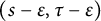 $(s-\varepsilon ,\tau -\varepsilon )$
to conclude that
$(s-\varepsilon ,\tau -\varepsilon )$
to conclude that
 $f_{s-\tau }=f_{(s-\varepsilon )-(\tau -\varepsilon )}$
is injective on
$f_{s-\tau }=f_{(s-\varepsilon )-(\tau -\varepsilon )}$
is injective on
 $(\overline \Sigma _{s-\varepsilon })^c$
. But Remark 3.18 tells us that every nonzero point in
$(\overline \Sigma _{s-\varepsilon })^c$
. But Remark 3.18 tells us that every nonzero point in
 $\overline \Sigma _{s-\varepsilon }$
is in
$\overline \Sigma _{s-\varepsilon }$
is in
 $\Sigma _s$
(and thus, not in
$\Sigma _s$
(and thus, not in
 $\partial \Sigma _s$
), under the condition (3.25). Thus, assuming
$\partial \Sigma _s$
), under the condition (3.25). Thus, assuming
 $0\notin \partial \Sigma _s$
, we find that injectivity of
$0\notin \partial \Sigma _s$
, we find that injectivity of
 $f_{s-\tau }$
extends to the boundary of
$f_{s-\tau }$
extends to the boundary of
 $\Sigma _s$
.
$\Sigma _s$
.
5 The boundary case
$\tau =0$

Recall from Definition 2.4 that a free multiplicative Brownian motion
 $b_{s,\tau }$
is defined for
$b_{s,\tau }$
is defined for
 $|s-\tau |\leq s$
. In this section, we focus on the borderline case of
$|s-\tau |\leq s$
. In this section, we focus on the borderline case of
 $\tau =0$
. Recall also from the discussion after Definition 2.4 that
$\tau =0$
. Recall also from the discussion after Definition 2.4 that
 $b_{s,0}$
is the free unitary Brownian motion
$b_{s,0}$
is the free unitary Brownian motion
 $U_s$
considered by Biane in [Reference Biane3]. Thus, we study
$U_s$
considered by Biane in [Reference Biane3]. Thus, we study
 $xb_{s,0}$
, where x is non-negative operator and freely independent of
$xb_{s,0}$
, where x is non-negative operator and freely independent of
 $b_{s,0}$
. The case in which
$b_{s,0}$
. The case in which
 $x=cI$
is special in that
$x=cI$
is special in that
 $xb_{s,0}$
is c times a unitary operator, so that the Brown measure of
$xb_{s,0}$
is c times a unitary operator, so that the Brown measure of
 $xb_{s,0}$
is supported on a circle of radius c centered at the origin.
$xb_{s,0}$
is supported on a circle of radius c centered at the origin.
Note that the domain
 $D_{s,0}$
from Definition 4.2 when
$D_{s,0}$
from Definition 4.2 when
 $\tau =0$
is defined by the relation
$\tau =0$
is defined by the relation
 $$\begin{align*}(D_{s,0})^c = f_{s}((\overline{\Sigma}_s)^c).\end{align*}$$
With
 $\tau =0$
, results from Theorem 4.2 can be stated as follows.
$\tau =0$
, results from Theorem 4.2 can be stated as follows.
Theorem 5.1 For a fixed
 $s> 0$
, we have:
$s> 0$
, we have:
-
• The map
$f_{s}: (\overline {\Sigma }_s)^c \rightarrow (D_{s,0})^c$
is injective. -
• The Brown measure
$\mu _{s,0}$
of
$xb_{s,0}$
is zero outside
$D_{s,0}$
except possibly at the origin.


Demni and Hamdi [Reference Demni and Hamdi8] carry out a PDE analysis for the regularized Brown measure of
 $xb_{s,0}$
, culminating in a formula [Reference Demni and Hamdi8, Theorem 1.1] analogous to our Theorem 4.4. In determining the support of the Brown measure, however, they specialize to the case in which x is a self-adjoint projection. See Theorem 1.2 in [Reference Demni and Hamdi8], where the authors are computing the Brown measure of the operator
$xb_{s,0}$
, culminating in a formula [Reference Demni and Hamdi8, Theorem 1.1] analogous to our Theorem 4.4. In determining the support of the Brown measure, however, they specialize to the case in which x is a self-adjoint projection. See Theorem 1.2 in [Reference Demni and Hamdi8], where the authors are computing the Brown measure of the operator
 $xb_{s,0}x$
in the compressed von Neumann algebra
$xb_{s,0}x$
in the compressed von Neumann algebra
 $x\mathcal A x$
, which is the same as the Brown measure of
$x\mathcal A x$
, which is the same as the Brown measure of
 $xb_{s,0}$
in
$xb_{s,0}$
in
 $\mathcal A$
, after removing an atom at the origin and multiplying by a constant. Our results therefore generalize [Reference Demni and Hamdi8] by treating arbitrary non-negative x and arbitrary
$\mathcal A$
, after removing an atom at the origin and multiplying by a constant. Our results therefore generalize [Reference Demni and Hamdi8] by treating arbitrary non-negative x and arbitrary
 $\tau $
with
$\tau $
with
 $\vert \tau -s\vert \leq s$
.
$\vert \tau -s\vert \leq s$
.
Demni and Hamdi first identify a domain
 $\Sigma _{t,\alpha }$
, where
$\Sigma _{t,\alpha }$
, where
 $\alpha $
is the trace of the projection x, which they show is bounded by a Jordan curve. Then, they define another domain
$\alpha $
is the trace of the projection x, which they show is bounded by a Jordan curve. Then, they define another domain
 $\Omega _{t,\alpha }$
whose boundary is the image of the boundary of
$\Omega _{t,\alpha }$
whose boundary is the image of the boundary of
 $\Sigma _{t,\alpha }$
under a map
$\Sigma _{t,\alpha }$
under a map
 $f_{t,\alpha }$
. Now, the map
$f_{t,\alpha }$
. Now, the map
 $f_{t,\alpha }$
in [Reference Demni and Hamdi8, Theorem 1.2] is easily seen to be what we call
$f_{t,\alpha }$
in [Reference Demni and Hamdi8, Theorem 1.2] is easily seen to be what we call
 $f_t$
. Meanwhile, the domain
$f_t$
. Meanwhile, the domain
 $\Sigma _{t,\alpha }$
in [Reference Demni and Hamdi8, Proposition 3.2] is defined by the condition
$\Sigma _{t,\alpha }$
in [Reference Demni and Hamdi8, Proposition 3.2] is defined by the condition
 $T_\alpha (\lambda _0)<t$
. Thus, if we can verify that their function
$T_\alpha (\lambda _0)<t$
. Thus, if we can verify that their function
 $T_\alpha $
agree with our T, then we will see that their
$T_\alpha $
agree with our T, then we will see that their
 $\Sigma _{t,\alpha }$
equals our
$\Sigma _{t,\alpha }$
equals our
 $\Sigma _t$
and thus that their
$\Sigma _t$
and thus that their
 $\Omega _{t,\alpha }$
is the interior of our
$\Omega _{t,\alpha }$
is the interior of our
 $D_{t,0}$
. Thus, their Theorem 1.2 will agree with Point 3 of our Theorem 4.2. (Recall that Demni and Hamdi remove the mass of the Brown measure at the origin.)
$D_{t,0}$
. Thus, their Theorem 1.2 will agree with Point 3 of our Theorem 4.2. (Recall that Demni and Hamdi remove the mass of the Brown measure at the origin.)
As depicted in Figures 7 and 8, the domain
 $D_{s,0}$
collapses onto the unit circle in the case when x is the identity operator (i.e.,
$D_{s,0}$
collapses onto the unit circle in the case when x is the identity operator (i.e.,
 $\mu =\delta _1$
), while no such collapse occurs when x is not a multiple of the identity (i.e.,
$\mu =\delta _1$
), while no such collapse occurs when x is not a multiple of the identity (i.e.,
 $\mu $
is not concentrated at a single point).
$\mu $
is not concentrated at a single point).

Figure 8: The domains
 $\overline \Sigma _s$
(left) and
$\overline \Sigma _s$
(left) and
 $D_{s,0}$
(right) with
$D_{s,0}$
(right) with
 $s=2$
and
$s=2$
and
 $\mu =0.5\,\delta _0+0.5\,\delta _1$
.
$\mu =0.5\,\delta _0+0.5\,\delta _1$
.
Proposition 5.2 The function
 $T_\alpha $
in [Reference Demni and Hamdi8, Proposition 2.10] agrees with our function T, when x is a self-adjoint projection with trace
$T_\alpha $
in [Reference Demni and Hamdi8, Proposition 2.10] agrees with our function T, when x is a self-adjoint projection with trace
 $\alpha $
.
$\alpha $
.
Proof By Proposition 2.10 in [Reference Demni and Hamdi8], we have that
 $$ \begin{align*} T_\alpha &= \frac{1}{2\dot{v}(0)}\log\left(1+ \frac{2\dot{v}(0)}{r_0^2\tau(q_0)}\right) \\ &= \frac{1}{1-\tilde{p}_\rho}\log\left(1+ \frac{1-\tilde{p}_\rho}{r_0^2\tilde{p}_0}\right), \end{align*} $$
where the first line uses the notation in [Reference Demni and Hamdi8] and the second line uses our notation from Section 3, where
 $\tilde {p}_\rho $
is the value of
$\tilde {p}_\rho $
is the value of
 $p_\rho $
at
$p_\rho $
at
 $\varepsilon _0=0$
. Thus, we only need to show that
$\varepsilon _0=0$
. Thus, we only need to show that
 $$\begin{align*}1-\tilde p_\rho = \tilde{p}_2 - \tilde{p}_0r_0^2.\end{align*}$$
But from (3.6), we have
 $$ \begin{align*} 1- \tilde{p}_\rho &= \operatorname{tr}\left[\frac{|x-\lambda_0|^2 - 2r^2_0 + 2xr_0\cos\theta}{|x-\lambda_0|^2}\right] \\ &= \operatorname{tr}\left[\frac{x^2 - 2xr_0\cos\theta + r_0^2 - 2r^2_0 + 2xr_0\cos\theta}{|x-\lambda_0|^2}\right] \\ &= \tilde{p}_2 - \tilde{p}_0r_0^2 \end{align*} $$
and the proof is complete.
Acknowledgements
The authors thank the referee for a careful reading of the article, which has led to several substantial improvements.


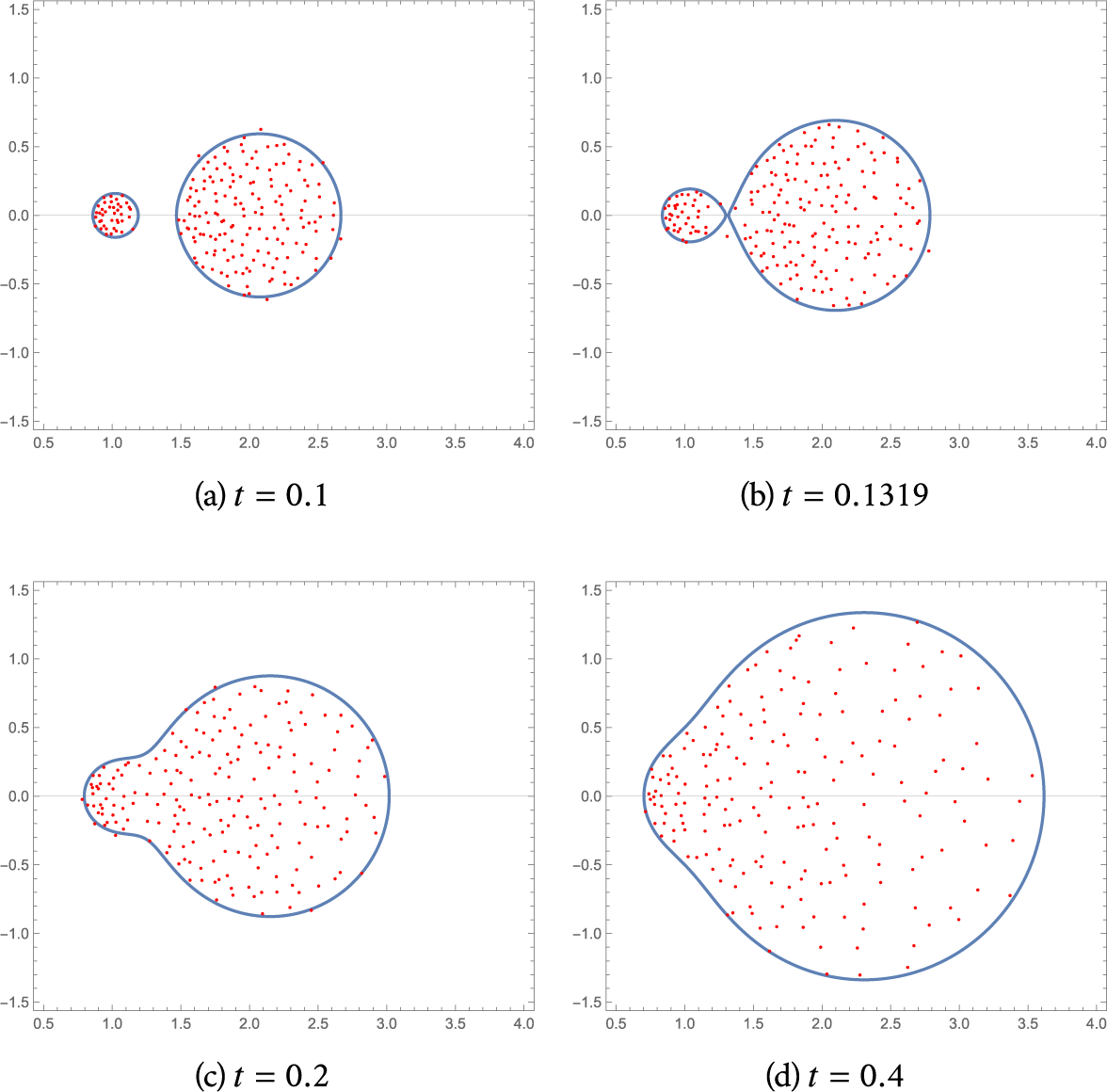


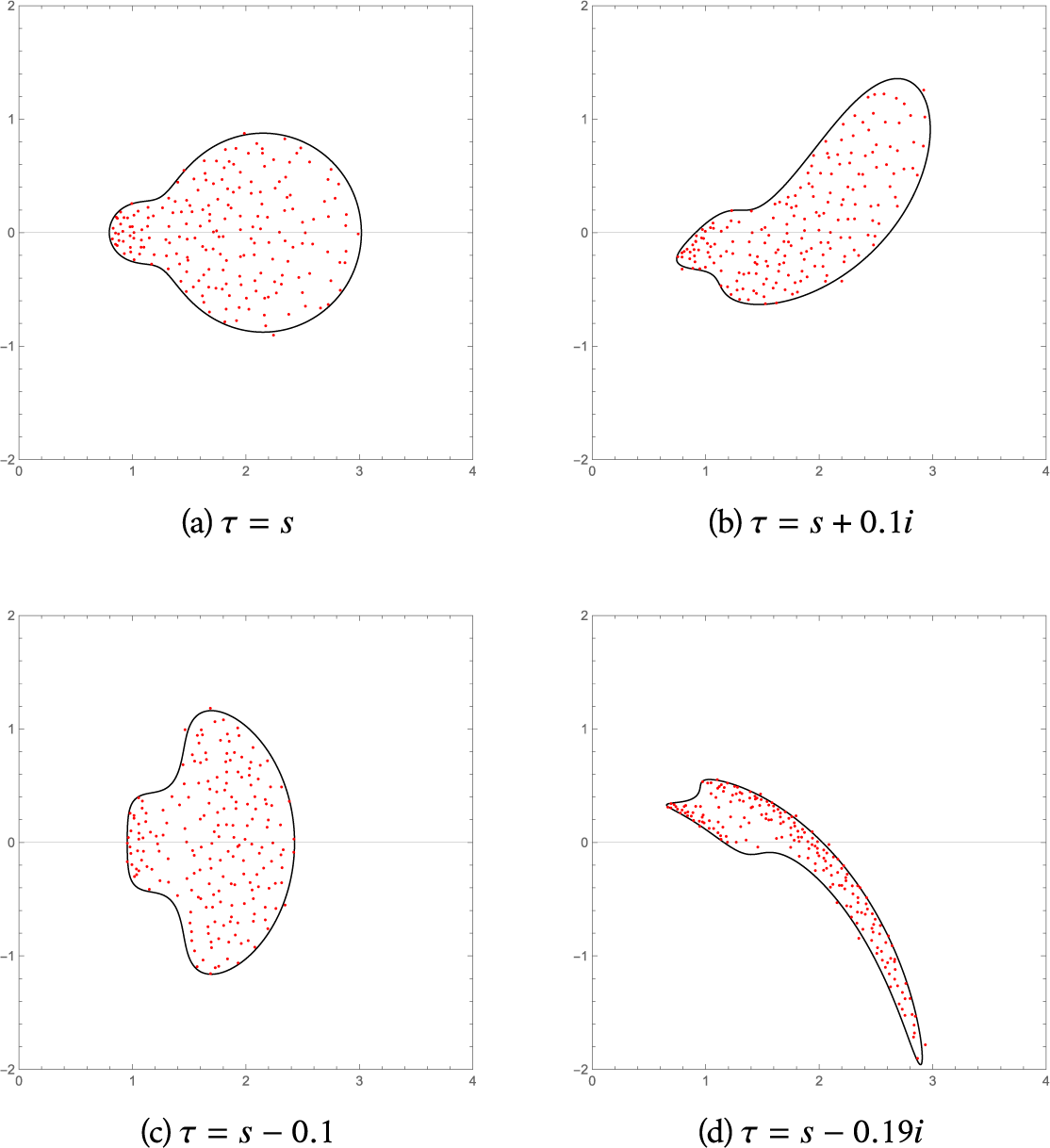


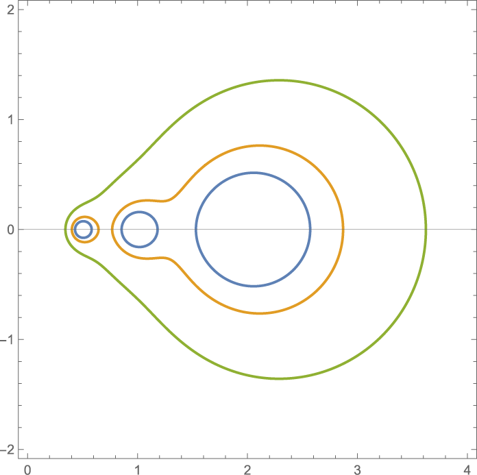


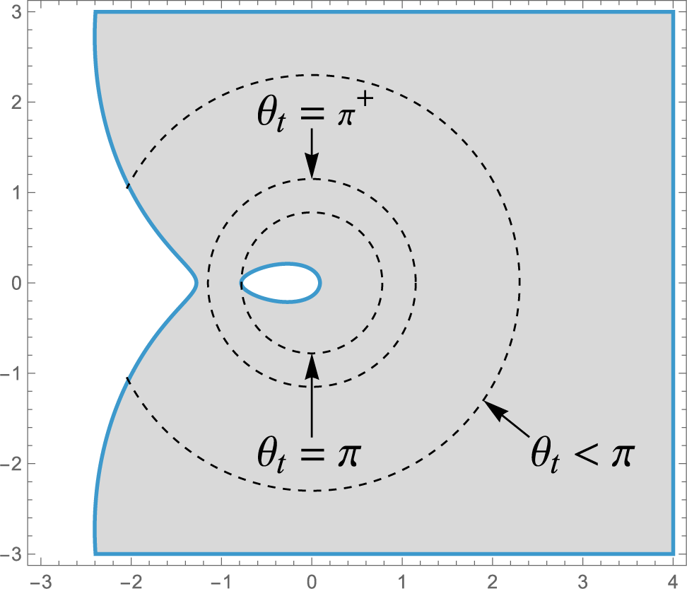


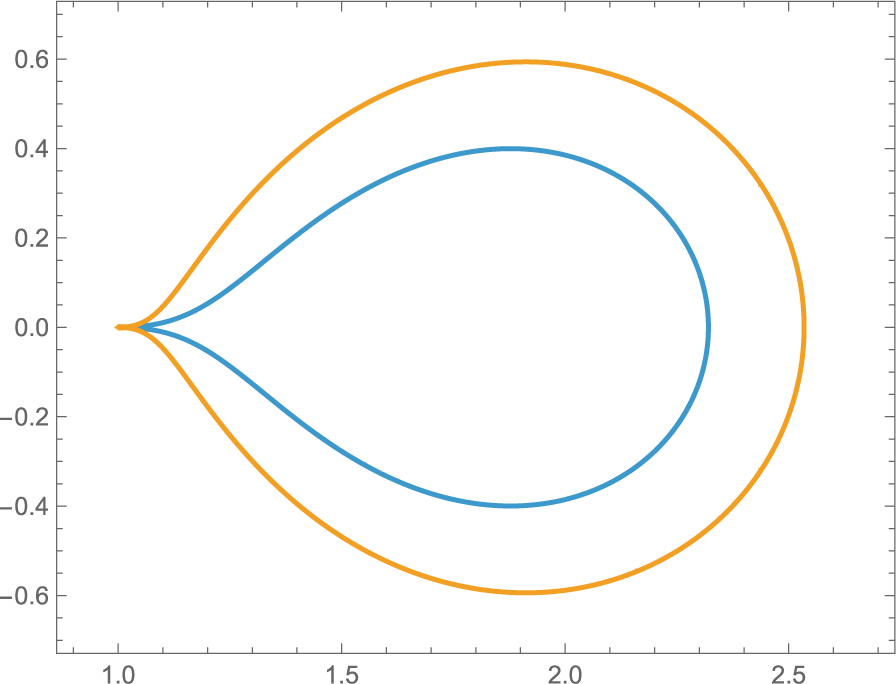


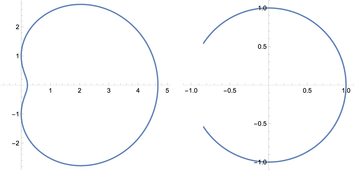


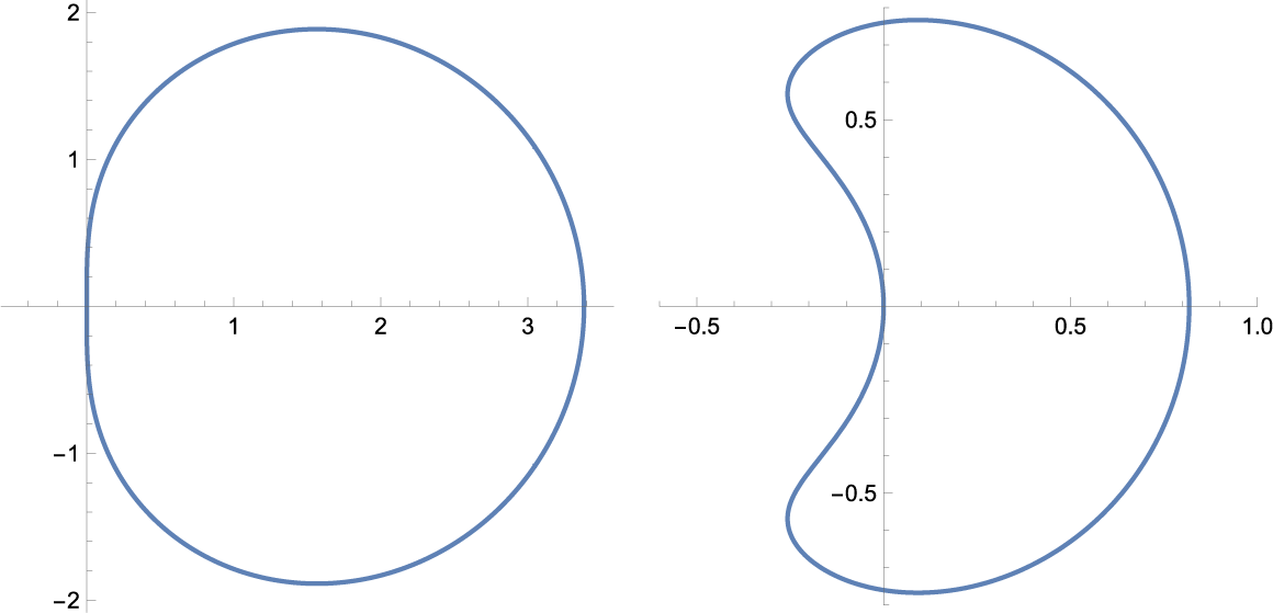


 Open access