


1. Introduction
One of the main obstacles to the successful operation of tokamak fusion reactors is plasma-terminating disruptions, caused by instabilities that lead to a sudden loss of plasma confinement. During such events, the plasma facing components can be damaged by high heat loads, and electromagnetic forces can cause significant mechanical stress on the machine (Hollmann et al. Reference Hollmann2015). Disruptions are characterised by a rapid drop in plasma temperature (thermal quench (TQ)), causing a subsequent, slower decrease in plasma current due to increased resistivity (current quench (CQ)), which in turn induces an electric field capable of accelerating electrons to relativistic speeds (Helander, Eriksson & Andersson Reference Helander, Eriksson and Andersson2002; Breizman et al. Reference Breizman, Aleynikov, Hollmann and Lehnen2019). One of the major challenges associated with disruptions is the generation of highly energetic runaway electron (RE) beams. If control of such an RE beam is lost, a large fraction of the stored energy can be deposited onto the first wall, sometimes in a highly localised impact area (Jepu et al. Reference Jepu2024).
This challenge is especially relevant for future devices such as SPARC and ITER, as the dominating RE generation mechanism, avalanche multiplication, is exponentially sensitive to the initial plasma current (Rosenbluth & Putvinski Reference Rosenbluth and Putvinski1997), which at full power will be 8.7 MA and 15 MA for SPARC and ITER, respectively. There are several proposed mitigation methods, most prominently massive material injection (MMI) of a combination of radiating impurities (e.g. Ne or Ar) and hydrogen isotopes, either in gaseous or solid state. In ITER, the reference concept for the disruption mitigation system is shattered pellet injection (SPI) (Baylor et al. Reference Baylor, Meitner, Gebhart, Caughman, Herfindal, Shiraki and Youchison2019). SPARC, however, will first deploy a simpler massive gas injection (MGI) system, and will additionally use a passive conducting coil with three-dimensional structure – the runaway electron mitigation coil (REMC) – acting to deconfine the REs faster than they are generated (Sweeney et al. Reference Sweeney2020).
RE mitigation in SPARC using MGI, both with and without the REMC, has been studied in previous works (Tinguely et al. Reference Tinguely2021; Izzo et al. Reference Izzo, Pusztai, Särkimäki, Sundström, Garnier, Weisberg, Tinguely, Paz-Soldan, Granetz and Sweeney2022; Tinguely et al. Reference Tinguely2023), and the addition of the REMC is shown to decrease the runaway current by several MAs. Runaway dynamics in ITER disruptions with MMI (both MGI and SPI) has been extensively studied by Vallhagen et al. (Reference Vallhagen, Embréus, Pusztai, Hesslow and Fülöp2020, Reference Vallhagen, Hanebring, Artola, Lehnen, Nardon, Fülöp, Hoppe, Newton and Pusztai2024). Similar studies have been performed for STEP (Spherical Tokamak for Energy Production) disruptions (Berger et al. Reference Berger, Pusztai, Newton, Hoppe, Vallhagen, Fil and Fülöp2022; Fil et al. Reference Fil, Henden, Newton, Hoppe and Vallhagen2024). In other works (Pusztai et al. Reference Pusztai, Ekmark, Bergström, Halldestam, Jansson, Hoppe, Vallhagen and Fülöp2023; Ekmark et al. Reference Ekmark, Hoppe, Fülöp, Jansson, Antonsson, Vallhagen and Pusztai2024), Bayesian optimisation was used to explore a large range of MMI density combinations for deuterium (D) and Ne in ITER. In addition to injected density magnitudes, Pusztai et al. (Reference Pusztai, Ekmark, Bergström, Halldestam, Jansson, Hoppe, Vallhagen and Fülöp2023) studied optimal radial distributions of the injected material. The main focus of the optimisation was to minimise the runaway current, but these works also considered figures of merits corresponding to heat loads from plasma particle transport and mechanical stresses from electromagnetic forces. None of these investigations found parameter regions with successful disruption mitigation for deuterium–tritium (DT) operation in ITER. However, there has been no such comprehensive exploration of the MMI injection density space for the compact, high-field device SPARC.
In this paper, we explore the space of injected D and noble gas densities in SPARC, without the effect of the REMC. Since simulations indicate that the REMC is capable of significantly mitigating the generation of a runaway current, we here aim to study disruption mitigation in SPARC without the REMC. This will isolate the mitigation effect of the MMI and give a conservative view of the success of the RE mitigation. The aim is to find parameter regions of favourable disruption mitigation and successful RE avoidance. Sample selection is done using Bayesian optimisation and the simulations are performed using the simulation tool Dream (Hoppe, Embréus & Fülöp Reference Hoppe, Embréus and Fülöp2021). More specifically, we employ the pitch-angle averaged kinetic model for superthermal electrons in Dream, which accurately captures the seed generation mechanisms (Ekmark et al. Reference Ekmark, Hoppe, Fülöp, Jansson, Antonsson, Vallhagen and Pusztai2024), yet it is sufficiently computationally inexpensive to allow numerical optimisation over a large parameter space.
2. Simulation set-up and plasma model
For the optimisation of disruption mitigation in SPARC, we have simulated disruption scenarios using the Dream code, developed especially for accurate and efficient studies of REs in fusion plasmas. In § 2.1, we describe how the SPARC disruptions have been modelled, while the electron and plasma parameter evolution is detailed in § 2.2, and the optimisation specifics are presented in § 2.3.
2.1. SPARC disruption scenario
We have initialised our disruption simulations with parameters corresponding to the SPARC primary reference discharge (Creely et al. Reference Creely2020), which has a plasma current ${I_{\textrm {p}}}={8.7}\, \textrm {MA}$
. The primary reference discharge is a DT (50–50 isotope mix) plasma, but we have also considered a pure D plasma with the same initial conditions. Notably, the assumptions of identical initial conditions for pure D and DT plasmas is somewhat simplistic, but enables us to compare the effects of Compton scattering and tritium beta decay on the runaway dynamics more easily. The initial plasma temperature, density and Ohmic current profiles from Rodriguez-Fernandez et al. (Reference Rodriguez-Fernandez, Howard, Greenwald, Creely, Hughes, Wright, Holland, Lin and Sciortino2020, Reference Rodriguez-Fernandez2022) used for the simulations are shown in figure 1(a). The electron and ion temperatures are initialised identically, but evolved separately. Furthermore, the equilibrium used has the on-axis magnetic field
${I_{\textrm {p}}}={8.7}\, \textrm {MA}$
. The primary reference discharge is a DT (50–50 isotope mix) plasma, but we have also considered a pure D plasma with the same initial conditions. Notably, the assumptions of identical initial conditions for pure D and DT plasmas is somewhat simplistic, but enables us to compare the effects of Compton scattering and tritium beta decay on the runaway dynamics more easily. The initial plasma temperature, density and Ohmic current profiles from Rodriguez-Fernandez et al. (Reference Rodriguez-Fernandez, Howard, Greenwald, Creely, Hughes, Wright, Holland, Lin and Sciortino2020, Reference Rodriguez-Fernandez2022) used for the simulations are shown in figure 1(a). The electron and ion temperatures are initialised identically, but evolved separately. Furthermore, the equilibrium used has the on-axis magnetic field $B_0={12.5}\, \textrm {T}$
,Footnote
1
major radius
$B_0={12.5}\, \textrm {T}$
,Footnote
1
major radius $R_0={1.89}\, \, \textrm {m}$
taken at the magnetic axis location and minor radius
$R_0={1.89}\, \, \textrm {m}$
taken at the magnetic axis location and minor radius $a={0.525} \, \textrm {m}$
, which have been obtained from FREEGS equilibrium simulations (Rodriguez-Fernandez et al. Reference Rodriguez-Fernandez, Howard, Greenwald, Creely, Hughes, Wright, Holland, Lin and Sciortino2020, Reference Rodriguez-Fernandez2022). In figure 1(b), the closed flux surfaces from the equilibrium simulations are plotted. The wall radius, which is a parameter in the boundary condition for Ampère’s law, was set to
$a={0.525} \, \textrm {m}$
, which have been obtained from FREEGS equilibrium simulations (Rodriguez-Fernandez et al. Reference Rodriguez-Fernandez, Howard, Greenwald, Creely, Hughes, Wright, Holland, Lin and Sciortino2020, Reference Rodriguez-Fernandez2022). In figure 1(b), the closed flux surfaces from the equilibrium simulations are plotted. The wall radius, which is a parameter in the boundary condition for Ampère’s law, was set to $b={0.621}\, \textrm {m}$
to match the available poloidal magnetic energy
$b={0.621}\, \textrm {m}$
to match the available poloidal magnetic energy $E_{\textrm {mag}}={52.3}\, \textrm {MJ}$
calculated using COMSOL by Tinguely et al. (Reference Tinguely2021), and the resistive wall time was set to 80 ms (Battey et al. Reference Battey, Hansen, Garnier, Weisberg, Paz-Soldan, Sweeney, Tinguely and Creely2023). As noted by Tinguely et al. (Reference Tinguely2021), the choice of wall radius does have an impact on the RE dynamics, but the qualitative optimisation results are not affected to the same degree, according to Ekmark et al. (Reference Ekmark, Hoppe, Fülöp, Jansson, Antonsson, Vallhagen and Pusztai2024). The evolution of the magnetic flux surface shaping and current density relaxation (Pusztai, Hoppe & Vallhagen Reference Pusztai, Hoppe and Vallhagen2022) during the TQ are not taken into account in the simulations.
$E_{\textrm {mag}}={52.3}\, \textrm {MJ}$
calculated using COMSOL by Tinguely et al. (Reference Tinguely2021), and the resistive wall time was set to 80 ms (Battey et al. Reference Battey, Hansen, Garnier, Weisberg, Paz-Soldan, Sweeney, Tinguely and Creely2023). As noted by Tinguely et al. (Reference Tinguely2021), the choice of wall radius does have an impact on the RE dynamics, but the qualitative optimisation results are not affected to the same degree, according to Ekmark et al. (Reference Ekmark, Hoppe, Fülöp, Jansson, Antonsson, Vallhagen and Pusztai2024). The evolution of the magnetic flux surface shaping and current density relaxation (Pusztai, Hoppe & Vallhagen Reference Pusztai, Hoppe and Vallhagen2022) during the TQ are not taken into account in the simulations.

Figure 1. Characteristics of the SPARC primary reference discharge. (a) Initial plasma temperature (solid blue), density (dash-dotted red) and Ohmic current density (dashed black) profiles. (b) Equilibrium flux surfaces (solid), plasma separatrix (dashed) and magnetic axis (cross). (c) Photon flux energy spectrum for a DT-plasma in SPARC with a total photon flux of ${1.4\times 10^{18}}\, {\, \textrm {m}^{-2}\ \textrm {s}^{-1}}$
(solid blue) and for a DD-plasma in SPARC with a total photon flux of
${1.4\times 10^{18}}\, {\, \textrm {m}^{-2}\ \textrm {s}^{-1}}$
(solid blue) and for a DD-plasma in SPARC with a total photon flux of ${3.3\times 10^{15}}\, {\, \textrm {m}^{-2}\, \textrm {s}^{-1}}$
(dashed black) compared with a DT-plasma in ITER with a total photon flux of
${3.3\times 10^{15}}\, {\, \textrm {m}^{-2}\, \textrm {s}^{-1}}$
(dashed black) compared with a DT-plasma in ITER with a total photon flux of ${10^{18}}\, {\, \textrm {m}^{-2}\, \textrm {s}^{-1}}$
(dash-dotted red).
${10^{18}}\, {\, \textrm {m}^{-2}\, \textrm {s}^{-1}}$
(dash-dotted red).
The disruption simulation is started with the deposition of D and noble gas (either He, Ne or Ar), instantly and uniformly across the plasma volume. During the disruption, the plasma heat losses are caused by convective losses of energetic electrons, heat conduction of the bulk electrons, as well as radiation which is more efficient at lower (below ${\sim} 100$
–
${\sim} 100$
– ${1000}\, \textrm {eV}$
) temperatures. The magnetic field stochastisation during the TQ cannot be modelled self-consistently in Dream. Instead, we employ spatially and temporally constant magnetic perturbations with a relative amplitude of
${1000}\, \textrm {eV}$
) temperatures. The magnetic field stochastisation during the TQ cannot be modelled self-consistently in Dream. Instead, we employ spatially and temporally constant magnetic perturbations with a relative amplitude of ${\delta B/B}={0.3}$
%, which was chosen to achieve a TQ duration of
${\delta B/B}={0.3}$
%, which was chosen to achieve a TQ duration of ${\sim} 0.1{-}1$
ms (Sweeney et al. Reference Sweeney2020) (the TQ time is presented for a few sample simulations in table 3). Note that the enforced transport due to magnetic perturbations is initialised simultaneously with the material deposition. The perturbations are active until the end of the TQ, which we define by the mean temperature falling below 20 eV.
${\sim} 0.1{-}1$
ms (Sweeney et al. Reference Sweeney2020) (the TQ time is presented for a few sample simulations in table 3). Note that the enforced transport due to magnetic perturbations is initialised simultaneously with the material deposition. The perturbations are active until the end of the TQ, which we define by the mean temperature falling below 20 eV.
During the TQ, the transport of superthermal electrons, REs and heat is calculated with the Rechester–Rosenbluth model (Rechester and Rosenbluth Reference Rechester and Rosenbluth1978), with the diffusion coefficient $D^{rr}\propto \left | v_\parallel \right | R_0({\delta B/B})^2$
. For the heat transport,
$D^{rr}\propto \left | v_\parallel \right | R_0({\delta B/B})^2$
. For the heat transport, $\left | v_\parallel \right |$
is replaced by the electron thermal speed and for the RE transport, by the speed of light. The Rechester–Rosenbluth model, however, does not account for the energy and angular dependence of the RE distribution, or for finite Larmor radius and orbit width effects (Särkimäki et al. Reference Särkimäki, Embreus, Nardon and Fülöp2020), but it gives an upper bound on the effect of the RE transport, as noted by Svensson et al. (Reference Svensson, Embreus, Newton, Särkimäki, Vallhagen and Fülöp2021) and Pusztai et al. (Reference Pusztai, Ekmark, Bergström, Halldestam, Jansson, Hoppe, Vallhagen and Fülöp2023).
$\left | v_\parallel \right |$
is replaced by the electron thermal speed and for the RE transport, by the speed of light. The Rechester–Rosenbluth model, however, does not account for the energy and angular dependence of the RE distribution, or for finite Larmor radius and orbit width effects (Särkimäki et al. Reference Särkimäki, Embreus, Nardon and Fülöp2020), but it gives an upper bound on the effect of the RE transport, as noted by Svensson et al. (Reference Svensson, Embreus, Newton, Särkimäki, Vallhagen and Fülöp2021) and Pusztai et al. (Reference Pusztai, Ekmark, Bergström, Halldestam, Jansson, Hoppe, Vallhagen and Fülöp2023).
Lower values of $\delta B/B$
reduce both the transported heat and RE losses. Yet the reduction in transported heat also slows the TQ temperature decay, thereby decreasing the hot-tail RE seed generation. Thus, the net effect of decreasing
$\delta B/B$
reduce both the transported heat and RE losses. Yet the reduction in transported heat also slows the TQ temperature decay, thereby decreasing the hot-tail RE seed generation. Thus, the net effect of decreasing $\delta B/B$
is, somewhat counter-intuitively, that the region of ‘safe’ MMI space increases. Simulations with a TQ duration
$\delta B/B$
is, somewhat counter-intuitively, that the region of ‘safe’ MMI space increases. Simulations with a TQ duration ${\gt} {3}\, \, \textrm {ms}$
are deemed to have an incomplete TQ, meaning that the amount of material that has been injected is not enough to cause a proper disruption. For such scenarios, we do not run the CQ simulation and instead penalise the sample with a high cost function value.
${\gt} {3}\, \, \textrm {ms}$
are deemed to have an incomplete TQ, meaning that the amount of material that has been injected is not enough to cause a proper disruption. For such scenarios, we do not run the CQ simulation and instead penalise the sample with a high cost function value.
As the magnetic flux surfaces are expected to heal after the TQ, the transport of superthermal electrons and REs is switched off during the CQ; however, a small heat transport, with ${\delta B/B}={0.04}$
% in accordance with previous works (Pusztai et al. Reference Pusztai, Ekmark, Bergström, Halldestam, Jansson, Hoppe, Vallhagen and Fülöp2023; Ekmark et al. Reference Ekmark, Hoppe, Fülöp, Jansson, Antonsson, Vallhagen and Pusztai2024), is retained to suppress the development of non-physical hot Ohmic current channels (Putvinski et al. Reference Putvinski, Fujisawa, Post, Putvinskaya, Rosenbluth and Wesley1997; Fehér et al. Reference Fehér, Smith, Fülöp and Gál2011). This transport level is orders of magnitude lower than the radiative heat losses at post-TQ temperatures, so it does not influence the evolution of the temperature and other plasma parameters.
${\delta B/B}={0.04}$
% in accordance with previous works (Pusztai et al. Reference Pusztai, Ekmark, Bergström, Halldestam, Jansson, Hoppe, Vallhagen and Fülöp2023; Ekmark et al. Reference Ekmark, Hoppe, Fülöp, Jansson, Antonsson, Vallhagen and Pusztai2024), is retained to suppress the development of non-physical hot Ohmic current channels (Putvinski et al. Reference Putvinski, Fujisawa, Post, Putvinskaya, Rosenbluth and Wesley1997; Fehér et al. Reference Fehér, Smith, Fülöp and Gál2011). This transport level is orders of magnitude lower than the radiative heat losses at post-TQ temperatures, so it does not influence the evolution of the temperature and other plasma parameters.
2.2. Electron dynamics and runaway modelling in Dream
Electrons in Dream (Hoppe et al. Reference Hoppe, Embréus and Fülöp2021) are divided into three populations – the thermal, superthermal and runaway populations – based on their momentum, and they are generally evolved using different models. Importantly, the superthermal electrons, with momenta $p\sim 0.01{-}1 \ {m_{\textrm {e}}} c$
(with
$p\sim 0.01{-}1 \ {m_{\textrm {e}}} c$
(with $m_{\textrm {e}}$
being the electron rest mass) of the same order of magnitude as the typical values for the critical momentum for RE generation, can be simulated using a kinetic model which has been analytically averaged over pitch-angle. Note that this pitch-angle averaged treatment is an accurate approximation at these moderate momenta, as the pitch-angle scattering is sufficiently strong to approximately isotropise the electron distribution. In this work, we have used this reduced kinetic model for the superthermal electrons, while the electrons in the thermal and runaway populations are modelled as fluids.
$m_{\textrm {e}}$
being the electron rest mass) of the same order of magnitude as the typical values for the critical momentum for RE generation, can be simulated using a kinetic model which has been analytically averaged over pitch-angle. Note that this pitch-angle averaged treatment is an accurate approximation at these moderate momenta, as the pitch-angle scattering is sufficiently strong to approximately isotropise the electron distribution. In this work, we have used this reduced kinetic model for the superthermal electrons, while the electrons in the thermal and runaway populations are modelled as fluids.
The advantage of this approach is that it greatly reduces the computational cost compared with fully kinetic simulations, while still enabling the runaway seed generation to be accurately simulated. Since the kinetic modelling of the seed generation entails more relaxed assumptions, it is typically more accurate than fluid modelling, especially in simulations with rapidly varying plasma parameters. The differences between fluid and kinetic treatment of the seed generation mechanisms can be quite significant, as shown by Ekmark et al. (Reference Ekmark, Hoppe, Fülöp, Jansson, Antonsson, Vallhagen and Pusztai2024).
The superthermal electrons will be described by their distribution function, from which relevant velocity moments, or fluid quantities, can be obtained, e.g. the superthermal electron density $n_{\textrm {st}}$
and current density
$n_{\textrm {st}}$
and current density $j_{\textrm {st}}$
. The distribution function,
$j_{\textrm {st}}$
. The distribution function, $f_{\textrm {st}}$
, will be evolved according to the bounce-averaged kinetic equation, derived in Appendix B.2. of Hoppe et al. (Reference Hoppe, Embréus and Fülöp2021) and referred to as the ‘isotropic’ model,
$f_{\textrm {st}}$
, will be evolved according to the bounce-averaged kinetic equation, derived in Appendix B.2. of Hoppe et al. (Reference Hoppe, Embréus and Fülöp2021) and referred to as the ‘isotropic’ model,
 \begin{align} \frac {\partial {f_{\textrm {st}}}}{\partial t}&= \frac {1}{p^2}\frac {\partial }{\partial p} \left [ p^2\left ( - A^p {f_{\textrm {st}}} + \hat {D}^{pp} \frac {\partial {f_{\textrm {st}}}}{\partial p} \right ) \right ] +\frac {1}{V^\prime }\frac {\partial }{\partial r}\left [ V^\prime D^{rr} \frac {\partial {f_{\textrm {st}}}}{\partial r} \right ]+ S_{\textrm {T}}+ S_{\textrm {C}}, \end{align}
where $V^\prime$
is the spatial Jacobian, and collisions are modelled by a test-particle Fokker–Planck operator. Note that the momentum
$V^\prime$
is the spatial Jacobian, and collisions are modelled by a test-particle Fokker–Planck operator. Note that the momentum $p$
is normalised to
$p$
is normalised to ${m_{\textrm {e}}} c$
. The distribution function is evolved for
${m_{\textrm {e}}} c$
. The distribution function is evolved for $p\in [0,\, p_{\textrm {re}}]$
, where we have chosen the upper momentum boundary as
$p\in [0,\, p_{\textrm {re}}]$
, where we have chosen the upper momentum boundary as $p_{\textrm {re}}=2.5\,{m_{\textrm {e}}} c$
and
$p_{\textrm {re}}=2.5\,{m_{\textrm {e}}} c$
and ${f_{\textrm {st}}}(p\gt p_{\textrm {re}})=0$
. In (2.1), the momentum advection term
${f_{\textrm {st}}}(p\gt p_{\textrm {re}})=0$
. In (2.1), the momentum advection term $A^p$
consists of slowing down due to the bremsstrahlung and collisions. Furthermore,
$A^p$
consists of slowing down due to the bremsstrahlung and collisions. Furthermore, $\hat {D}^{pp}=D^{pp}+\mathcal{D}_E$
, where
$\hat {D}^{pp}=D^{pp}+\mathcal{D}_E$
, where $D^{pp}$
is the diffusive component of the collision operator and
$D^{pp}$
is the diffusive component of the collision operator and $\mathcal{D}_E\propto (e\boldsymbol{E}\cdot \boldsymbol{B})^2/( B^2 \nu _{\textrm {D}})$
describes the effect of the electric field in the presence of strong pitch-angle scattering, with the pitch-angle scattering collision frequency
$\mathcal{D}_E\propto (e\boldsymbol{E}\cdot \boldsymbol{B})^2/( B^2 \nu _{\textrm {D}})$
describes the effect of the electric field in the presence of strong pitch-angle scattering, with the pitch-angle scattering collision frequency $\nu _{\textrm {D}}=\nu _{\textrm {D}}(p)$
. The radial diffusion
$\nu _{\textrm {D}}=\nu _{\textrm {D}}(p)$
. The radial diffusion $D^{rr}$
is evaluated using the Rechester–Rosenbluth model (Rechester and Rosenbluth Reference Rechester and Rosenbluth1978).
$D^{rr}$
is evaluated using the Rechester–Rosenbluth model (Rechester and Rosenbluth Reference Rechester and Rosenbluth1978).
The source term
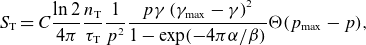 \begin{align} S_{\textrm {T}} &= C\frac {\ln 2}{4\pi } \frac {n_{\textrm {T}}}{\tau _{\textrm {T}}}\frac {1}{p^2} \frac {p \gamma \left (\gamma _{\textrm {max}}-\gamma \right )^2}{1-\exp (-4\pi \alpha /\beta )} \Theta (p_{\textrm {max}} - p), \end{align}
describes the generation of superthermal electrons from tritium beta decay, derived by Ekmark et al. (Reference Ekmark, Hoppe, Fülöp, Jansson, Antonsson, Vallhagen and Pusztai2024). In (2.2), the fine structure constant $\alpha \approx 1/137$
and
$\alpha \approx 1/137$
and $C$
is a normalisation constant used to ensure that the integrated source yields the T decay rate
$C$
is a normalisation constant used to ensure that the integrated source yields the T decay rate $(\ln 2)\, n_{\textrm {T}}/\tau _{\textrm {T}}$
, where
$(\ln 2)\, n_{\textrm {T}}/\tau _{\textrm {T}}$
, where $\tau _{\textrm {T}}\approx 4500$
days is the half-life for T and
$\tau _{\textrm {T}}\approx 4500$
days is the half-life for T and $n_{\textrm {T}}$
is the T density. Additionally,
$n_{\textrm {T}}$
is the T density. Additionally, $\gamma =\sqrt {p^2+1}$
is the Lorentz factor and
$\gamma =\sqrt {p^2+1}$
is the Lorentz factor and $\beta =p/\gamma$
is the normalised speed. During tritium beta decay, electrons will be generated with a kinetic energy
$\beta =p/\gamma$
is the normalised speed. During tritium beta decay, electrons will be generated with a kinetic energy $W\in [0,\ W_{\textrm {max}}]$
, with
$W\in [0,\ W_{\textrm {max}}]$
, with $W_{\textrm {max}}={18.6}\, \textrm {keV}$
determining
$W_{\textrm {max}}={18.6}\, \textrm {keV}$
determining $p_{\textrm {max}}$
and
$p_{\textrm {max}}$
and $\gamma _{\textrm {max}}$
.
$\gamma _{\textrm {max}}$
.
The generation of superthermal electrons from Compton scattering due to photons emitted from the walls during activated operation is described by (Ekmark et al. Reference Ekmark, Hoppe, Fülöp, Jansson, Antonsson, Vallhagen and Pusztai2024)
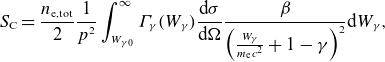 \begin{align} S_{\textrm {C}} &= \frac {n_{\textrm {e,tot}}}{2}\frac {1}{p^2}\int _{W_{\gamma 0}}^\infty \varGamma _\gamma (W_\gamma ) \frac {\textrm {d} \sigma }{\textrm {d} \Omega } \frac {\beta }{\left (\frac {W_\gamma }{{m_{\textrm {e}}} c^2}+1-\gamma \right )^2}\textrm {d} W_\gamma , \end{align}
where $n_{\textrm {e,tot}}$
is the total electron density in the plasma and
$n_{\textrm {e,tot}}$
is the total electron density in the plasma and $\textrm {d} \sigma / \textrm {d} \Omega$
is the Klein–Nishina differential cross-section (Klein & Nishina Reference Klein and Nishina1929). Here, the photon flux energy spectrum
$\textrm {d} \sigma / \textrm {d} \Omega$
is the Klein–Nishina differential cross-section (Klein & Nishina Reference Klein and Nishina1929). Here, the photon flux energy spectrum
 \begin{equation} \varGamma _\gamma (W_\gamma ) =\varGamma _{\textrm {flux}}\exp [-\exp (-z)-z+1]\left /\int \exp [-\exp (-z)-z+1]\, \textrm {d} W_\gamma, \right. \end{equation}
where $z = [\ln (W_\gamma \ [\textrm {MeV}])+C_1]/C_2+C_3(W_\gamma \ [\textrm {MeV}])^2$
, is based on the functional form used for ITER by Martín-Solís et al. (Reference Martín-Solís, Loarte and Lehnen2017). The
$z = [\ln (W_\gamma \ [\textrm {MeV}])+C_1]/C_2+C_3(W_\gamma \ [\textrm {MeV}])^2$
, is based on the functional form used for ITER by Martín-Solís et al. (Reference Martín-Solís, Loarte and Lehnen2017). The $W_\gamma ^2$
-term in the expression for
$W_\gamma ^2$
-term in the expression for $z$
is added to the form used by Martín-Solís et al. (Reference Martín-Solís, Loarte and Lehnen2017) to achieve a steeper decrease for higher photon energies, in accordance with the photon energy spectrum data used for the fit of the parameters
$z$
is added to the form used by Martín-Solís et al. (Reference Martín-Solís, Loarte and Lehnen2017) to achieve a steeper decrease for higher photon energies, in accordance with the photon energy spectrum data used for the fit of the parameters $C_1$
,
$C_1$
, $C_2$
and
$C_2$
and $C_3$
.
$C_3$
.
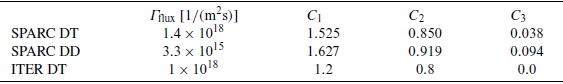
The data for the photon energy spectrum are preliminary results obtained from Monte Carlo N-Particle Transport (MCNP) calculations by Commonwealth Fusion Systems, and the photon energy spectrum is plotted in figure 1(c) together with the ITER spectrum. Note that despite SPARC having a lower fusion power than ITER, its much smaller size causes the total photon fluxes to be similar – for both, $\varGamma _{\textrm {flux}}\sim {10^{18}}\, {\textrm {m}^{-2}\, \textrm {s}^{-1}}$
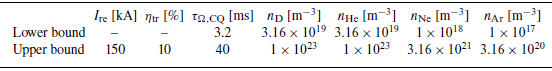
. The parameters used to represent the photon flux spectrum for both DT and D operation are presented in table 1, together with the corresponding ITER parameters. We have assumed that the flux from the activated walls reduces by a factor of
$\varGamma _{\textrm {flux}}\sim {10^{18}}\, {\textrm {m}^{-2}\, \textrm {s}^{-1}}$
. The parameters used to represent the photon flux spectrum for both DT and D operation are presented in table 1, together with the corresponding ITER parameters. We have assumed that the flux from the activated walls reduces by a factor of $10^4$
after the TQ when the fusion reactions, and corresponding neutron generation, cease.
$10^4$
after the TQ when the fusion reactions, and corresponding neutron generation, cease.
Table 1. Total photon flux and fitted photon flux spectrum parameters used for the source term for energetic electrons generated by Compton scattering. The corresponding photon flux spectra are plotted in figure 1(c). The photon flux spectrum parameters were obtained by fitting data from MCNP calculations.
The runaway electrons will be evolved through their particle density $n_{\textrm {re}}$
, according to (Hoppe et al. Reference Hoppe, Embréus and Fülöp2021)
$n_{\textrm {re}}$
, according to (Hoppe et al. Reference Hoppe, Embréus and Fülöp2021)
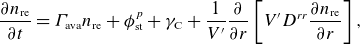 \begin{align} \frac {\partial {n_{\textrm {re}}}}{\partial t}&=\varGamma _{\textrm {ava}}{n_{\textrm {re}}}+\phi _{\textrm {st}}^p+\gamma _{\textrm {C}} +\frac {1}{V^\prime }\frac {\partial }{\partial r}\left [ V^\prime D^{rr} \frac {\partial {n_{\textrm {re}}}}{\partial r} \right ], \end{align}
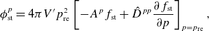 \begin{align} \phi _{\textrm {st}}^p&= 4\pi V' p_{\textrm {re}}^2\left [ - A^p {f_{\textrm {st}}} + \hat {D}^{pp}\frac {\partial {f_{\textrm {st}}}}{\partial p} \right ]_{p=p_{\textrm {re}}}, \end{align}
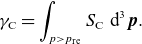 \begin{align} \gamma _{\textrm {C}}&=\int _{p\gt p_{\textrm {re}}}S_{\textrm {C}}\ \textrm {d}^3\boldsymbol{p}.\\[8pt]\nonumber \end{align}
Here, the avalanche growth rate $\varGamma _{\textrm {ava}}$
is determined by the model of Hesslow et al. (Reference Hesslow, Embréus, Vallhagen and Fülöp2019), and the radial transport by the Rechester–Rosenbluth model (Rechester and Rosenbluth Reference Rechester and Rosenbluth1978) through
$\varGamma _{\textrm {ava}}$
is determined by the model of Hesslow et al. (Reference Hesslow, Embréus, Vallhagen and Fülöp2019), and the radial transport by the Rechester–Rosenbluth model (Rechester and Rosenbluth Reference Rechester and Rosenbluth1978) through $D^{rr}$
. The flux of particles
$D^{rr}$
. The flux of particles $\phi _{\textrm {st}}^p$
from the superthermal population is determined by the momentum space flux through the upper boundary
$\phi _{\textrm {st}}^p$
from the superthermal population is determined by the momentum space flux through the upper boundary $p_{\textrm {re}}$
of the superthermal grid, on which the superthermal distribution function is defined. This momentum space flux naturally includes the RE source generation categorised as Dreicer generation and hot-tail generation, as well as the generation of REs from Compton scattering and tritium beta decay with
$p_{\textrm {re}}$
of the superthermal grid, on which the superthermal distribution function is defined. This momentum space flux naturally includes the RE source generation categorised as Dreicer generation and hot-tail generation, as well as the generation of REs from Compton scattering and tritium beta decay with $p\lt p_{\textrm {re}}$
. Compton scattering will also generate REs with
$p\lt p_{\textrm {re}}$
. Compton scattering will also generate REs with $p\gt p_{\textrm {re}}$
, which is accounted for with
$p\gt p_{\textrm {re}}$
, which is accounted for with $\gamma _{\textrm {C}}$
. Note that the same is not true for tritium beta decay, as we have chosen
$\gamma _{\textrm {C}}$
. Note that the same is not true for tritium beta decay, as we have chosen $p_{\textrm {re}}$
such that
$p_{\textrm {re}}$
such that $p_{\textrm {max}}\lt p_{\textrm {re}}$
. The REs will be assumed to travel at the speed of light, which is typically valid in reactor-scale tokamak disruptions, yielding the current density
$p_{\textrm {max}}\lt p_{\textrm {re}}$
. The REs will be assumed to travel at the speed of light, which is typically valid in reactor-scale tokamak disruptions, yielding the current density $j_{\textrm {re}}={n_{\textrm {re}}} e c$
as supported by Buchholz (Reference Buchholz2023).
$j_{\textrm {re}}={n_{\textrm {re}}} e c$
as supported by Buchholz (Reference Buchholz2023).
The thermal electrons will be represented by their density $n_{\textrm {th}}$
, temperature
$n_{\textrm {th}}$
, temperature $T_{\textrm {th}}$
and the Ohmic current density
$T_{\textrm {th}}$
and the Ohmic current density $j_\Omega$
. Quasineutrality is used to constrain the thermal density, i.e.
$j_\Omega$
. Quasineutrality is used to constrain the thermal density, i.e. ${n_{\textrm {th}}}=n_{\textrm {free}} - {n_{\textrm {st}}} - {n_{\textrm {re}}}$
, while the Ohmic current density is evolved through
${n_{\textrm {th}}}=n_{\textrm {free}} - {n_{\textrm {st}}} - {n_{\textrm {re}}}$
, while the Ohmic current density is evolved through ${j_\Omega }=\sigma (\boldsymbol{E}\cdot \boldsymbol{B})/B$
. For the electrical conductivity
${j_\Omega }=\sigma (\boldsymbol{E}\cdot \boldsymbol{B})/B$
. For the electrical conductivity $\sigma$
, we use the Sauter–Redl formula (Redl et al. Reference Redl, Angioni, Belli and Sauter2021), which accounts for trapping effects. The temperature
$\sigma$
, we use the Sauter–Redl formula (Redl et al. Reference Redl, Angioni, Belli and Sauter2021), which accounts for trapping effects. The temperature $T_{\textrm {th}}$
is evolved through the thermal energy
$T_{\textrm {th}}$
is evolved through the thermal energy $W_{\textrm {th}}=3{n_{\textrm {th}}}{T_{\textrm {th}}}/2$
, according to (Hoppe et al. Reference Hoppe, Embréus and Fülöp2021)
$W_{\textrm {th}}=3{n_{\textrm {th}}}{T_{\textrm {th}}}/2$
, according to (Hoppe et al. Reference Hoppe, Embréus and Fülöp2021)
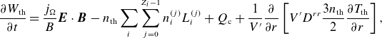 \begin{equation} \frac {\partial W_{\textrm {th}}}{\partial t}= \frac {{j_\Omega }}{B}\boldsymbol{E}\cdot \boldsymbol{B}-{n_{\textrm {th}}}\sum _i\sum _{j=0}^{Z_i-1}n_i^{(j)}L_i^{(j)} + Q_{\textrm {c}} + \frac {1}{V^\prime }\frac {\partial }{\partial r}\left [ V^\prime D^{rr}\frac {3{n_{\textrm {th}}}}2\frac {\partial {T_{\textrm {th}}}}{\partial r}\right ], \end{equation}
and outside of the plasma, ${T_{\textrm {th}}}(r\gt a)=0$
. The first term of (2.6) models the Ohmic heating, and the third term heating from collisions with ions and non-thermal electrons, while the fourth accounts for the radial transport. Energy loss due to inelastic atomic processes are accounted for in the second term for each atomic species
${T_{\textrm {th}}}(r\gt a)=0$
. The first term of (2.6) models the Ohmic heating, and the third term heating from collisions with ions and non-thermal electrons, while the fourth accounts for the radial transport. Energy loss due to inelastic atomic processes are accounted for in the second term for each atomic species $i$
with atomic number
$i$
with atomic number $Z_i$
, namely line, recombination and bremsstrahlung radiation, as well as changes in potential energy due to ionisation and recombination, all encompassed by the effective rate coefficient
$Z_i$
, namely line, recombination and bremsstrahlung radiation, as well as changes in potential energy due to ionisation and recombination, all encompassed by the effective rate coefficient $L_i^{(j)}$
. The ionisation, recombination and radiation rates are taken from the ADAS database for the noble gases. For the hydrogen isotopes, data from the AMJUEL database (Reiter Reference Reiter2020) are used instead, to account for opacity to Lyman radiation. This has been shown to be important at high D densities (Vallhagen et al. Reference Vallhagen, Embréus, Pusztai, Hesslow and Fülöp2020, Reference Vallhagen, Pusztai, Hoppe, Newton and Fülöp2022).
$L_i^{(j)}$
. The ionisation, recombination and radiation rates are taken from the ADAS database for the noble gases. For the hydrogen isotopes, data from the AMJUEL database (Reiter Reference Reiter2020) are used instead, to account for opacity to Lyman radiation. This has been shown to be important at high D densities (Vallhagen et al. Reference Vallhagen, Embréus, Pusztai, Hesslow and Fülöp2020, Reference Vallhagen, Pusztai, Hoppe, Newton and Fülöp2022).
2.3. Disruption optimisation for SPARC
As figures of merit for quantifying the efficiency of the disruption mitigation, we use a combination of the runaway current $I_{\textrm {re}}$
, fraction of heat transported to the plasma facing components
$I_{\textrm {re}}$
, fraction of heat transported to the plasma facing components $\eta _{\textrm {tr}}$
(including heat loss through the convective losses of superthermal electrons and heat conduction of the bulk electrons) and CQ time
$\eta _{\textrm {tr}}$
(including heat loss through the convective losses of superthermal electrons and heat conduction of the bulk electrons) and CQ time $\tau _{\Omega ,\textrm {CQ}}$
, in accordance with previous studies (Pusztai et al. Reference Pusztai, Ekmark, Bergström, Halldestam, Jansson, Hoppe, Vallhagen and Fülöp2023; Ekmark et al. Reference Ekmark, Hoppe, Fülöp, Jansson, Antonsson, Vallhagen and Pusztai2024). Both the runaway current and the transported heat load fraction should be minimised to avoid damage to the plasma facing components. More specifically, a transported heat load fraction, i.e. the fraction of the initial plasma kinetic energy which has been lost from the plasma due to energy transport, of less than 10 % would be desirable during a disruption (Hollmann et al. Reference Hollmann2015). Regarding the runaway current, there is no strict upper limit, but a runaway current of less than 150 kA, as previously used for ITER (Pusztai et al. Reference Pusztai, Ekmark, Bergström, Halldestam, Jansson, Hoppe, Vallhagen and Fülöp2023; Ekmark et al. Reference Ekmark, Hoppe, Fülöp, Jansson, Antonsson, Vallhagen and Pusztai2024), would be ideal, while even a runaway current of up to 1 MA might be tolerable. Note that the plasma facing components in SPARC are not actively cooled. The risks posed by runaway strikes are tile surface degradation and the production of impurities that may affect subsequent plasmas. The runaway current has been quantified by its value at the time when it reaches 95 % of the remaining total plasma current (
$\tau _{\Omega ,\textrm {CQ}}$
, in accordance with previous studies (Pusztai et al. Reference Pusztai, Ekmark, Bergström, Halldestam, Jansson, Hoppe, Vallhagen and Fülöp2023; Ekmark et al. Reference Ekmark, Hoppe, Fülöp, Jansson, Antonsson, Vallhagen and Pusztai2024). Both the runaway current and the transported heat load fraction should be minimised to avoid damage to the plasma facing components. More specifically, a transported heat load fraction, i.e. the fraction of the initial plasma kinetic energy which has been lost from the plasma due to energy transport, of less than 10 % would be desirable during a disruption (Hollmann et al. Reference Hollmann2015). Regarding the runaway current, there is no strict upper limit, but a runaway current of less than 150 kA, as previously used for ITER (Pusztai et al. Reference Pusztai, Ekmark, Bergström, Halldestam, Jansson, Hoppe, Vallhagen and Fülöp2023; Ekmark et al. Reference Ekmark, Hoppe, Fülöp, Jansson, Antonsson, Vallhagen and Pusztai2024), would be ideal, while even a runaway current of up to 1 MA might be tolerable. Note that the plasma facing components in SPARC are not actively cooled. The risks posed by runaway strikes are tile surface degradation and the production of impurities that may affect subsequent plasmas. The runaway current has been quantified by its value at the time when it reaches 95 % of the remaining total plasma current ( $I_{\textrm {re}}(t_{I_{\textrm {re}}=0.95{I_{\textrm {p}}}})$
), unless this happens after the occurrence of the maximum runaway current (
$I_{\textrm {re}}(t_{I_{\textrm {re}}=0.95{I_{\textrm {p}}}})$
), unless this happens after the occurrence of the maximum runaway current ( $I_{\textrm {re}}=\max _tI_{\textrm {re}}$
), in which case, the latter will be used, as motivated in Appendix A.1 of Ekmark et al. (Reference Ekmark, Hoppe, Fülöp, Jansson, Antonsson, Vallhagen and Pusztai2024).
$I_{\textrm {re}}=\max _tI_{\textrm {re}}$
), in which case, the latter will be used, as motivated in Appendix A.1 of Ekmark et al. (Reference Ekmark, Hoppe, Fülöp, Jansson, Antonsson, Vallhagen and Pusztai2024).
The duration of the CQ, or CQ time, is also an important metric, as too short CQ times can lead to mechanical stresses due to induced eddy currents in the plasma surrounding structures, while too long CQ times can lead to intolerably large halo currents in plasma facing components. In SPARC, the range of tolerable CQ times is expected to be bounded from below and above by 3.2 ms (Sweeney et al. Reference Sweeney2020) and 40 ms according to the ITPA Disruption Database (Eidietis et al. Reference Eidietis2015). The lower bound of 3.2 ms has been chosen because all SPARC components are designed to withstand an exponential CQ with characteristic decay time $\tau ={1.385}\, \textrm {ms}$
(equivalent to a 3.2 ms linear CQ following the ITPA 80 %–20 % convention). Furthermore, using the ITPA 80 %–20 % convention, we evaluate the CQ time through extrapolation, i.e.
$\tau ={1.385}\, \textrm {ms}$
(equivalent to a 3.2 ms linear CQ following the ITPA 80 %–20 % convention). Furthermore, using the ITPA 80 %–20 % convention, we evaluate the CQ time through extrapolation, i.e. ${\tau _{\Omega ,\textrm {CQ}}}=(t_{{I_\Omega }=0.2{I_{\textrm {p}}^{t=0}}}-t_{{I_\Omega }=0.8{I_{\textrm {p}}^{t=0}}})/0.6$
if the Ohmic current drops below 20 % of the initial plasma current (
${\tau _{\Omega ,\textrm {CQ}}}=(t_{{I_\Omega }=0.2{I_{\textrm {p}}^{t=0}}}-t_{{I_\Omega }=0.8{I_{\textrm {p}}^{t=0}}})/0.6$
if the Ohmic current drops below 20 % of the initial plasma current ( ${I_{\textrm {p}}^{t=0}}={8.7}\, \textrm {MA}$
) during the simulation and, otherwise,
${I_{\textrm {p}}^{t=0}}={8.7}\, \textrm {MA}$
) during the simulation and, otherwise, ${\tau _{\Omega ,\textrm {CQ}}}=(t_{\textrm {final}}- t_{{I_\Omega }=0.8{I_{\textrm {p}}^{t=0}}})/(0.8-{I_\Omega ^{\textrm {final}}}/{I_{\textrm {p}}^{t=0}})$
. Note that we denote the CQ time
${\tau _{\Omega ,\textrm {CQ}}}=(t_{\textrm {final}}- t_{{I_\Omega }=0.8{I_{\textrm {p}}^{t=0}}})/(0.8-{I_\Omega ^{\textrm {final}}}/{I_{\textrm {p}}^{t=0}})$
. Note that we denote the CQ time $\tau _{\Omega ,\textrm {CQ}}$
to signify that this CQ time corresponds to the decay of the Ohmic current, rather than the total plasma current. Additionally, to avoid favouring simulations with an incomplete CQ, we also want to minimise the final Ohmic current in the cost function. Furthermore, a high final Ohmic current has the potential to be converted into runaway current, and thus introduces an uncertainty for such disruptions.
$\tau _{\Omega ,\textrm {CQ}}$
to signify that this CQ time corresponds to the decay of the Ohmic current, rather than the total plasma current. Additionally, to avoid favouring simulations with an incomplete CQ, we also want to minimise the final Ohmic current in the cost function. Furthermore, a high final Ohmic current has the potential to be converted into runaway current, and thus introduces an uncertainty for such disruptions.
We use the same cost function $\mathcal{L}$
as that devised by Ekmark et al. (Reference Ekmark, Hoppe, Fülöp, Jansson, Antonsson, Vallhagen and Pusztai2024), which was designed with the main aim of distinguishing between successful (
$\mathcal{L}$
as that devised by Ekmark et al. (Reference Ekmark, Hoppe, Fülöp, Jansson, Antonsson, Vallhagen and Pusztai2024), which was designed with the main aim of distinguishing between successful ( ${\mathcal{L}}\lt 1$
) and unsuccessful (
${\mathcal{L}}\lt 1$
) and unsuccessful ( ${\mathcal{L}}\gt 1$
) disruption mitigation. It takes the form
${\mathcal{L}}\gt 1$
) disruption mitigation. It takes the form
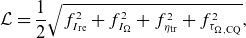 \begin{align} {\mathcal{L}}&=\frac 12\sqrt {f_{I_{\textrm {re}}}^2+f_{I_\Omega }^2 + f_{\eta _{\textrm {tr}}}^2+f_{\tau _{\Omega ,\textrm {CQ}}}^2}, \end{align}
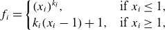 \begin{align} f_i&= \begin{cases} (x_i)^{k_i}, &\text{if } x_i\leq 1,\\ k_i(x_i-1)+1, &\text{if } x_i\geq 1, \end{cases}\\[8pt]\nonumber \end{align}
where $x_I=I/{150}\, \textrm {kA}$
and
$x_I=I/{150}\, \textrm {kA}$
and $x_{\eta _{\textrm {tr}}}={\eta _{\textrm {tr}}}/{10}\, \%$
, since they should be minimised. For the CQ time, the goal is not to minimise it, but rather to contain it within a certain interval and, therefore, we use
$x_{\eta _{\textrm {tr}}}={\eta _{\textrm {tr}}}/{10}\, \%$
, since they should be minimised. For the CQ time, the goal is not to minimise it, but rather to contain it within a certain interval and, therefore, we use $x_{\tau _{\Omega ,\textrm {CQ}}}=\left | {\tau _{\Omega ,\textrm {CQ}}}-{21.6}\, \textrm {ms} \right |/{18.4}\, \textrm {ms}$
. Using this form causes the optimal value of
$x_{\tau _{\Omega ,\textrm {CQ}}}=\left | {\tau _{\Omega ,\textrm {CQ}}}-{21.6}\, \textrm {ms} \right |/{18.4}\, \textrm {ms}$
. Using this form causes the optimal value of $\tau _{\Omega ,\textrm {CQ}}$
to be located at the middle of the interval at
$\tau _{\Omega ,\textrm {CQ}}$
to be located at the middle of the interval at $(3.2+40)/2={21.6}\, \textrm {ms}$
, but in reality, it is not necessarily better to have, e.g.
$(3.2+40)/2={21.6}\, \textrm {ms}$
, but in reality, it is not necessarily better to have, e.g. ${\tau _{\Omega ,\textrm {CQ}}}={20}\, \textrm {ms}$
than
${\tau _{\Omega ,\textrm {CQ}}}={20}\, \textrm {ms}$
than ${\tau _{\Omega ,\textrm {CQ}}}={10}\, \textrm {ms}$
. For this reason, we use
${\tau _{\Omega ,\textrm {CQ}}}={10}\, \textrm {ms}$
. For this reason, we use $k_{\tau _{\Omega ,\textrm {CQ}}}=6$
, as for CQ times well within the interval of safety,
$k_{\tau _{\Omega ,\textrm {CQ}}}=6$
, as for CQ times well within the interval of safety, $f_{\tau _{\Omega ,\textrm {CQ}}}\ll 1$
. Furthermore, we use
$f_{\tau _{\Omega ,\textrm {CQ}}}\ll 1$
. Furthermore, we use $k_I=1$
for the currents and
$k_I=1$
for the currents and $k_{\eta _{\textrm {tr}}}=3$
for the transported heat loss. Thus, using the form (2.7b) ensures that, when all the cost function values are within their acceptable limits, minimising the currents will be favoured over minimising the transported heat loss, which in turn will be favoured over having
$k_{\eta _{\textrm {tr}}}=3$
for the transported heat loss. Thus, using the form (2.7b) ensures that, when all the cost function values are within their acceptable limits, minimising the currents will be favoured over minimising the transported heat loss, which in turn will be favoured over having $\tau _{\Omega ,\textrm {CQ}}$
close to 21.6 ms.
$\tau _{\Omega ,\textrm {CQ}}$
close to 21.6 ms.
To avoid unnecessarily long simulations, the Dream simulations are stopped when all the cost function quantities can be determined and only vary negligibly with time. More specifically, this happens when ${I_\Omega }\lt 0.2{I_{\textrm {p}}^{t=0}}$
and either
${I_\Omega }\lt 0.2{I_{\textrm {p}}^{t=0}}$
and either $I_{\textrm {re}}^{95\,\%}$
or
$I_{\textrm {re}}^{95\,\%}$
or $I_{\textrm {re}}^{\textrm {max}}$
has occurred. Additionally, we require that either
$I_{\textrm {re}}^{\textrm {max}}$
has occurred. Additionally, we require that either ${I_\Omega }\lt {100}\, \textrm {kA}$
at the end of the simulation or that we have simulated for longer than
${I_\Omega }\lt {100}\, \textrm {kA}$
at the end of the simulation or that we have simulated for longer than $2{\tau _{\Omega ,\textrm {CQ}}}$
. The simulation will also be terminated if
$2{\tau _{\Omega ,\textrm {CQ}}}$
. The simulation will also be terminated if $I_{\textrm {re}}\lt {150}\, \textrm {kA}$
and
$I_{\textrm {re}}\lt {150}\, \textrm {kA}$
and ${I_\Omega }\lt {100}\, \textrm {kA}$
, even though neither of
${I_\Omega }\lt {100}\, \textrm {kA}$
, even though neither of $I_{\textrm {re}}^{95\,\%}$
and
$I_{\textrm {re}}^{95\,\%}$
and $I_{\textrm {re}}^{\textrm {max}}$
has occurred. Using these termination conditions means that the final Ohmic current will not play a big role in how the cost function varies, as for most simulations, it will be
$I_{\textrm {re}}^{\textrm {max}}$
has occurred. Using these termination conditions means that the final Ohmic current will not play a big role in how the cost function varies, as for most simulations, it will be ${\sim} {100}\, \textrm {kA}$
. It will only play a significant role if
${\sim} {100}\, \textrm {kA}$
. It will only play a significant role if ${I_\Omega }\gg {150}\, \textrm {kA}$
. Another consequence of this is that
${I_\Omega }\gg {150}\, \textrm {kA}$
. Another consequence of this is that ${\mathcal{L}}\geq 0.5\times ({100}\, \textrm {kA}) / ({150}\, \textrm {kA})\approx 0.33$
, which does limit the interpretability of the cost function for low cost function values, but this was deemed less important than the efficiency gain of using such termination conditions.
${\mathcal{L}}\geq 0.5\times ({100}\, \textrm {kA}) / ({150}\, \textrm {kA})\approx 0.33$
, which does limit the interpretability of the cost function for low cost function values, but this was deemed less important than the efficiency gain of using such termination conditions.
The optimisation parameters are the densities of the injected material, notably using logarithmic scales to enable studying MMI densities over several orders of magnitude. The optimisation bounds can be found in table 2 together with the limits of safety for the disruption figures of merit. In SPARC, the current MGI design allows for injected quantities resulting in D densities ${\lt} {4.8\times10^{22}}\, {\, \textrm {m}^{-3}}$
, and Ne and Ar densities
${\lt} {4.8\times10^{22}}\, {\, \textrm {m}^{-3}}$
, and Ne and Ar densities ${\lt} {4.7\times 10^{21}}\, {\, \textrm {m}^{-3}}$
, while currently there is no plan to use He as an MGI gas. These upper design limits of the densities have been evaluated under the assumption that the injected gas is distributed uniformly in the whole vacuum vessel, with a volume of 45
${\lt} {4.7\times 10^{21}}\, {\, \textrm {m}^{-3}}$
, while currently there is no plan to use He as an MGI gas. These upper design limits of the densities have been evaluated under the assumption that the injected gas is distributed uniformly in the whole vacuum vessel, with a volume of 45 $\, \textrm {m}^3$
. In fact, the upper design limits regard injected particle numbers, not particle densities, and arise from the fuel processing. Since we only simulate the plasma, with a plasma volume of 20 m
$\, \textrm {m}^3$
. In fact, the upper design limits regard injected particle numbers, not particle densities, and arise from the fuel processing. Since we only simulate the plasma, with a plasma volume of 20 m $^3$
, assuming uniform distribution of the injected material means that the nominal upper bound corresponds to 44 % assimilation of D. In ASDEX Upgrade, assimilation of 40 % has been reached, making this a reasonable limit to consider (Pautasso et al. Reference Pautasso, Mlynek, Bernert, Mank, Herrmann, Dux, Müller, Scarabosio and Sertoli2015). Thus notably, while our optimisation will explore noble gas densities within their allowed ranges, we explore higher D densities than will be possible to achieve, according to the current design. Optimisations have been performed for disruptions during D operation caused by D and Ne injections, as well as disruptions during DT operation caused by D in combination with Ne, Ar or He injections. For each optimisation, 400 simulations have been performed.
$^3$
, assuming uniform distribution of the injected material means that the nominal upper bound corresponds to 44 % assimilation of D. In ASDEX Upgrade, assimilation of 40 % has been reached, making this a reasonable limit to consider (Pautasso et al. Reference Pautasso, Mlynek, Bernert, Mank, Herrmann, Dux, Müller, Scarabosio and Sertoli2015). Thus notably, while our optimisation will explore noble gas densities within their allowed ranges, we explore higher D densities than will be possible to achieve, according to the current design. Optimisations have been performed for disruptions during D operation caused by D and Ne injections, as well as disruptions during DT operation caused by D in combination with Ne, Ar or He injections. For each optimisation, 400 simulations have been performed.
Table 2. Bounds for successful mitigation of the disruption figures of merit used for the cost function, as well as the bounds used for the injected material densities in the optimisations.
In this work, we have used a Bayesian optimisation strategy using Gaussian processes, meaning that it is assumed that the nature of the random variables involved is Gaussian. Bayesian optimisation is advantageous, compared with e.g. a grid scan, since regions of interest are well resolved, while less computational resources are focused on simulations corresponding to poor disruption mitigation. In Bayesian optimisation, inference based on Bayesian statistics is used to evaluate a probability distribution function for the cost function based on a set of samples. Through this probability density function, an estimation for the cost function landscape can be obtained through the mean of the probability density $\mu$
and an error estimate can be obtained from the covariance. Furthermore, an acquisition function is needed to determine how to choose new samples during the optimisation and for this, we have used the expected improvement acquisition function, which chooses the sample that maximises the expected improvement. Here, the Bayesian optimisation was performed using the Python package by Nogueira (Reference Nogueira2014). For the Gaussian processes, the Matérn covariance kernel with smoothness parameter
$\mu$
and an error estimate can be obtained from the covariance. Furthermore, an acquisition function is needed to determine how to choose new samples during the optimisation and for this, we have used the expected improvement acquisition function, which chooses the sample that maximises the expected improvement. Here, the Bayesian optimisation was performed using the Python package by Nogueira (Reference Nogueira2014). For the Gaussian processes, the Matérn covariance kernel with smoothness parameter $\nu =3/2$
was used.
$\nu =3/2$
was used.
3. Disruption mitigation optimisation
Here, we present the results from the disruption mitigation optimisation with regards to the MMI densities. In § 3.1, we optimise disruption mitigation for a pure D plasma using MMI of D and Ne. We consider cases with and without generation of REs from Compton scattering due to photon flux from the DD neutron bombardment of the wall. In § 3.2, we instead focus on DT operation, and then account for REs generated both from Compton scattering and tritium beta decay. For disruptions of DT plasmas, aside from Ne, we also consider He and Ar MMI in combination with D.
3.1. Deuterium operation
For pure D plasmas, the RE generation from Compton scattering is often neglected due to the low neutron energy of the neutronic DD reaction and low cross-section of the DD fusion reaction (Pusztai et al. Reference Pusztai, Ekmark, Bergström, Halldestam, Jansson, Hoppe, Vallhagen and Fülöp2023; Ekmark et al. Reference Ekmark, Hoppe, Fülöp, Jansson, Antonsson, Vallhagen and Pusztai2024). When the RE seed is only generated by hot-tail and Dreicer generation, it is easier to suppress the formation of a significant runaway current, making the mitigation of such scenarios more attainable. In this section, we have optimised the MMI densities of D and Ne for pure D plasmas, both with and without the Compton seed.
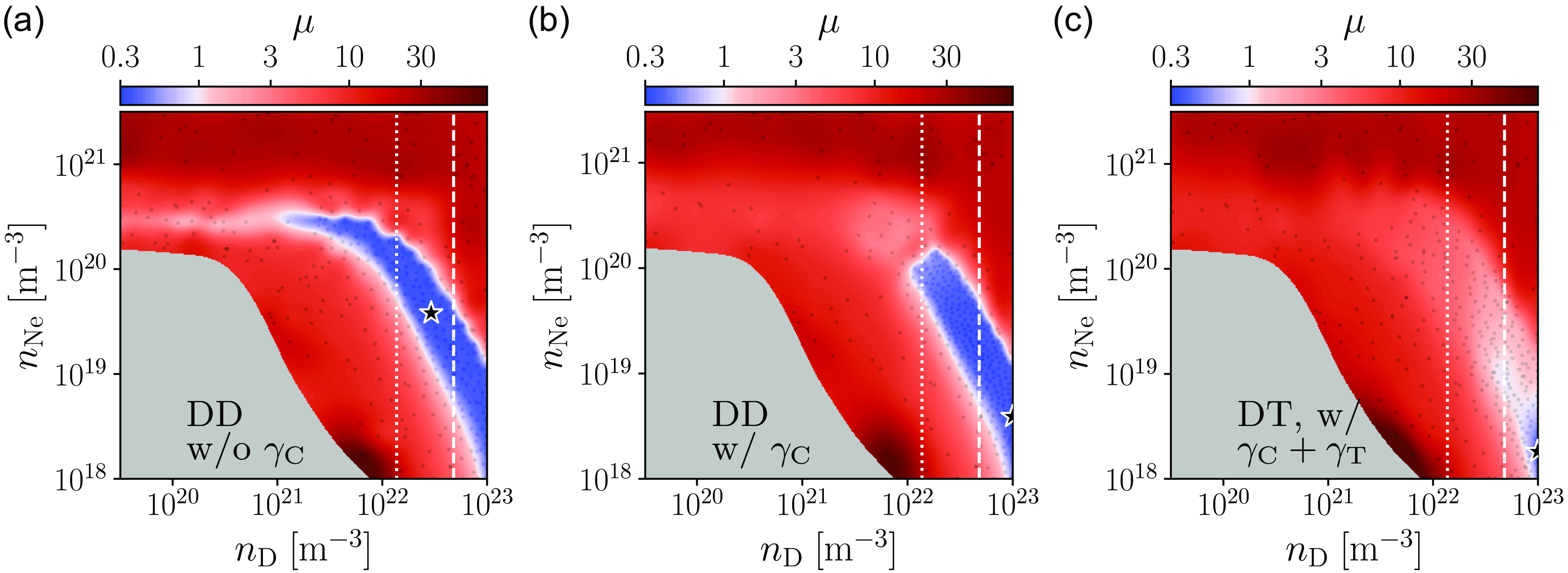
Figure 2. Logarithmic contour plots of the cost function estimate $\mu$
for D operation (a) without Compton generation and (b) with DD-induced Compton generation, as well as (c) for DT operation with RE generation from both DT-induced Compton scattering and tritium beta decay. Note that the colour mapping is adapted such that blue shades represent regions of safe operation. The black star indicates the optimal samples, while the black dots indicate all optimisation samples, and the upper design limit of the D density during MGI in SPARC is indicated by the dashed vertical line for 44 % assimilation (
$\mu$
for D operation (a) without Compton generation and (b) with DD-induced Compton generation, as well as (c) for DT operation with RE generation from both DT-induced Compton scattering and tritium beta decay. Note that the colour mapping is adapted such that blue shades represent regions of safe operation. The black star indicates the optimal samples, while the black dots indicate all optimisation samples, and the upper design limit of the D density during MGI in SPARC is indicated by the dashed vertical line for 44 % assimilation ( ${n_{\textrm {D}}}={4.8\times 10^{22}}\, {\, \textrm {m}^{-3}}$
) and the dotted vertical line for 10 % assimilation. The grey area covers the region of incomplete TQ.
${n_{\textrm {D}}}={4.8\times 10^{22}}\, {\, \textrm {m}^{-3}}$
) and the dotted vertical line for 10 % assimilation. The grey area covers the region of incomplete TQ.
The estimated cost function landscape obtained from the optimisation samples without generation from Compton scattering is shown in figure 2(a). There is a relatively large band of successful disruption mitigation scenarios, as indicated by the blue shaded region in the plot, which stretches from ${n_{\textrm {D}}}\sim {10^{21}}\, {\, \textrm {m}^{-3}}$
and
${n_{\textrm {D}}}\sim {10^{21}}\, {\, \textrm {m}^{-3}}$
and ${n_{\textrm {Ne}}}\sim {3\times 10^{20}}\, {\, \textrm {m}^{-3}}$
to
${n_{\textrm {Ne}}}\sim {3\times 10^{20}}\, {\, \textrm {m}^{-3}}$
to ${n_{\textrm {D}}}\sim {10^{23}}\, {\, \textrm {m}^{-3}}$
and
${n_{\textrm {D}}}\sim {10^{23}}\, {\, \textrm {m}^{-3}}$
and ${n_{\textrm {Ne}}}\sim {3\times 10^{18}}\, {\, \textrm {m}^{-3}}$
. Parts of this safe region even stretch below the upper design limit with 10 % assimilation. As indicated by the deep blue shade of this region of safety, the majority of this region has
${n_{\textrm {Ne}}}\sim {3\times 10^{18}}\, {\, \textrm {m}^{-3}}$
. Parts of this safe region even stretch below the upper design limit with 10 % assimilation. As indicated by the deep blue shade of this region of safety, the majority of this region has $\mu \approx 0.3$
, which is the lower bound for the cost function due to the termination conditions we use for the CQ simulation, as discussed in § 2.3. Thus, for the major part of the safe region, the final Ohmic current dominates the cost function values. The optimum can be found in the middle of this safe region at
$\mu \approx 0.3$
, which is the lower bound for the cost function due to the termination conditions we use for the CQ simulation, as discussed in § 2.3. Thus, for the major part of the safe region, the final Ohmic current dominates the cost function values. The optimum can be found in the middle of this safe region at ${n_{\textrm {D}}}\approx {2.9\times 10^{22}}\, {\, \textrm {m}^{-3}}$
and
${n_{\textrm {D}}}\approx {2.9\times 10^{22}}\, {\, \textrm {m}^{-3}}$
and ${n_{\textrm {Ne}}}\approx {3.8\times 10^{19}}\, {\textrm {m}^{-3}}$
, corresponding to 27 % assimilation of the upper design limit. At this optimal sample, no runaway current is generated, while
${n_{\textrm {Ne}}}\approx {3.8\times 10^{19}}\, {\textrm {m}^{-3}}$
, corresponding to 27 % assimilation of the upper design limit. At this optimal sample, no runaway current is generated, while ${\tau _{\Omega ,\textrm {CQ}}}\approx {7.8}\, \textrm {ms}$
and
${\tau _{\Omega ,\textrm {CQ}}}\approx {7.8}\, \textrm {ms}$
and ${\eta _{\textrm {tr}}}\approx {4.5}$
%, meaning that all the figures of merit we use to quantify the disruption are well within their limits of safe operation.
${\eta _{\textrm {tr}}}\approx {4.5}$
%, meaning that all the figures of merit we use to quantify the disruption are well within their limits of safe operation.
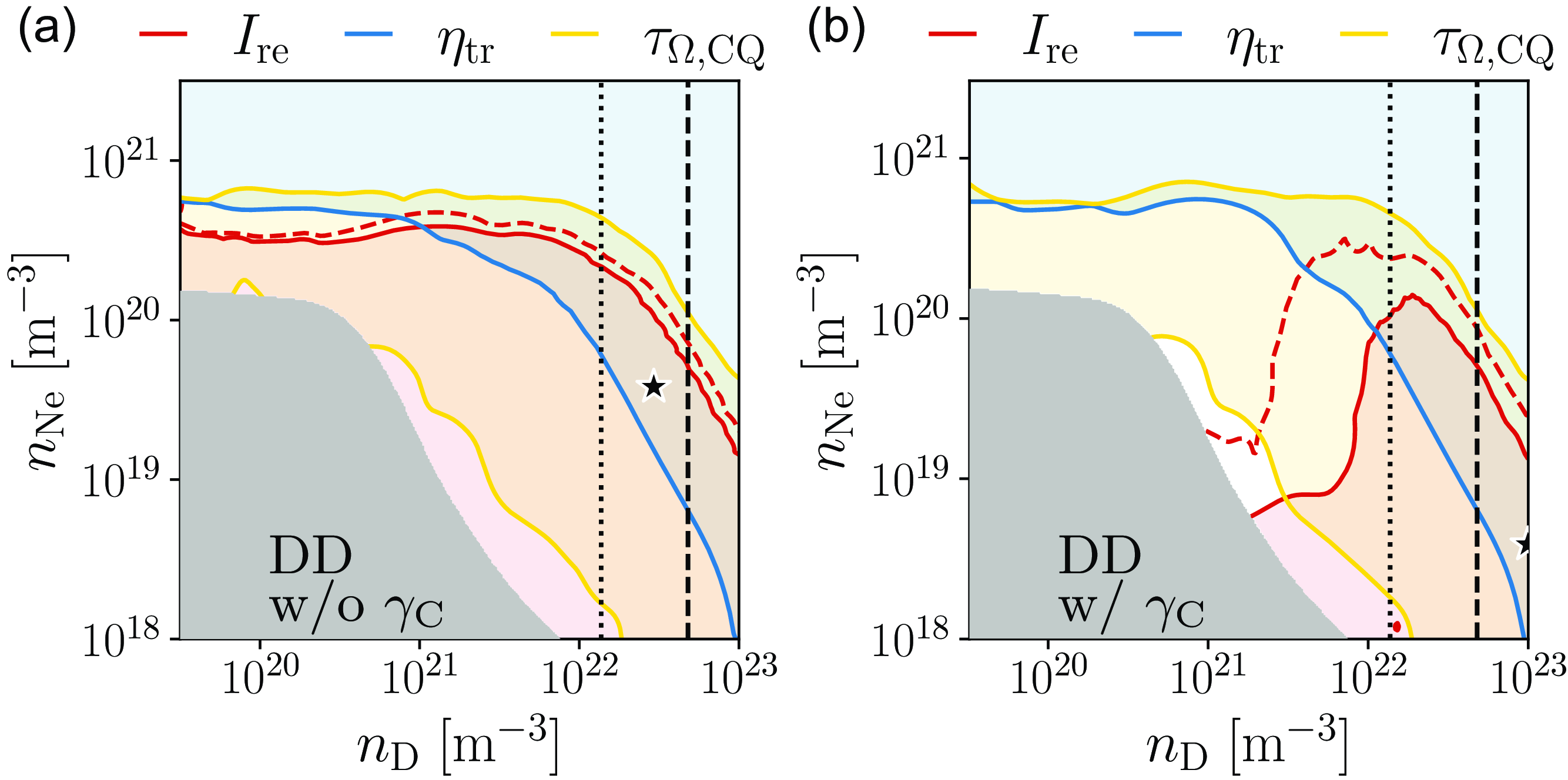
Figure 3. Regions of safe operation (shaded) with regards to $I_{\textrm {re}}$
(red),
$I_{\textrm {re}}$
(red), $\eta _{\textrm {tr}}$
(blue) and
$\eta _{\textrm {tr}}$
(blue) and $\tau _{\Omega ,\textrm {CQ}}$
(yellow) for D operation (a) without Compton generation and (b) with Compton generation. Additionally, the red dashed line indicates where the runaway current is 1 MA, bounding the tolerable region of operation. The optimal sample is indicated by a star, the upper design limit of the D density during MGI in SPARC is indicated by the dashed vertical line for 44 % assimilation (
$\tau _{\Omega ,\textrm {CQ}}$
(yellow) for D operation (a) without Compton generation and (b) with Compton generation. Additionally, the red dashed line indicates where the runaway current is 1 MA, bounding the tolerable region of operation. The optimal sample is indicated by a star, the upper design limit of the D density during MGI in SPARC is indicated by the dashed vertical line for 44 % assimilation ( ${n_{\textrm {D}}}={4.8\times 10^{22}}\, {\rm m^{-3}}$
) and the dotted vertical line for 10 % assimilation. The grey area covers the region of incomplete TQ.
${n_{\textrm {D}}}={4.8\times 10^{22}}\, {\rm m^{-3}}$
) and the dotted vertical line for 10 % assimilation. The grey area covers the region of incomplete TQ.
In figure 3(a), the regions of safe operation for each individual figure of merit across the explored density space in figure 2(a) are shown, that is, for the optimisation of D operation without Compton generation. The more detailed landscapes of the runaway current, transported heat loss and CQ time are presented in figure 8(a) in Appendix A. The safe region for the runaway current corresponds to lower Ne densities and spans approximately the lower half of the explored density space. Close to the boundary of this safe region, the gradient in density space is very high, as the contour line for $I_{\textrm {re}}={150}\, \textrm {kA}$
(solid red) and the one for
$I_{\textrm {re}}={150}\, \textrm {kA}$
(solid red) and the one for $I_{\textrm {re}}={1}\, \textrm {MA}$
(dashed red) are very close to each other. Thus, increasing the Ne density slightly around this boundary will cause a sharp increase in the RE density. However, for high values of the MMI densities, the transported heat fraction is within its limit of safe operation – the region of
$I_{\textrm {re}}={1}\, \textrm {MA}$
(dashed red) are very close to each other. Thus, increasing the Ne density slightly around this boundary will cause a sharp increase in the RE density. However, for high values of the MMI densities, the transported heat fraction is within its limit of safe operation – the region of ${\eta _{\textrm {tr}}}\lt {10}$
% covers the upper right portion of the explored density space.
${\eta _{\textrm {tr}}}\lt {10}$
% covers the upper right portion of the explored density space.
When RE generation from DD neutron-induced Compton scattering is considered, the region of safe operation decreases at high Ne densities (figure 2
b) as the regions of $I_{\textrm {re}}\lt {150}\, \textrm {kA}$
and
$I_{\textrm {re}}\lt {150}\, \textrm {kA}$
and $I_{\textrm {re}}\lt {1}\, \textrm {MA}$
shrink (figure 3
b). More specifically, for the region in injected-material-density space corresponding to successful mitigation, the lower boundary for the D density is increased by an order of magnitude, while the upper boundary for the Ne denstity is decreased by a factor of
$I_{\textrm {re}}\lt {1}\, \textrm {MA}$
shrink (figure 3
b). More specifically, for the region in injected-material-density space corresponding to successful mitigation, the lower boundary for the D density is increased by an order of magnitude, while the upper boundary for the Ne denstity is decreased by a factor of ${\sim} 2.5$
. The location of the optimum found is significantly different to that of the optimum found when disregarding Compton generation; however, this is due to the cost function value being
${\sim} 2.5$
. The location of the optimum found is significantly different to that of the optimum found when disregarding Compton generation; however, this is due to the cost function value being ${\sim} 0.35$
along the valley of the blue region of figure 2(b). Thus, when accounting for Compton generation, the optimum in figure 2(a) is equivalently successful in terms of mitigation to the optimum in figure 2(b). With RE generation from Compton scattering, there is also a larger separation between the contour lines of
${\sim} 0.35$
along the valley of the blue region of figure 2(b). Thus, when accounting for Compton generation, the optimum in figure 2(a) is equivalently successful in terms of mitigation to the optimum in figure 2(b). With RE generation from Compton scattering, there is also a larger separation between the contour lines of $I_{\textrm {re}}={150}\, \textrm {kA}$
and
$I_{\textrm {re}}={150}\, \textrm {kA}$
and $I_{\textrm {re}}={1}\, \textrm {MA}$
(red solid and dashed in figure 3(b), respectively). Thus, even during D operation, Compton scattering can have a significant impact on the disruption dynamics. Furthermore, this informs us that Compton scattering will play an important role during DT operation, as the photon flux will be significantly larger then (see table 1).
$I_{\textrm {re}}={1}\, \textrm {MA}$
(red solid and dashed in figure 3(b), respectively). Thus, even during D operation, Compton scattering can have a significant impact on the disruption dynamics. Furthermore, this informs us that Compton scattering will play an important role during DT operation, as the photon flux will be significantly larger then (see table 1).
3.2. Deuterium–tritium operation
Disruptions are expected to be more difficult to mitigate during DT operation, due to the generation of REs from DT-induced Compton scattering, which is expected to be more severe than DD-induced generation due to the neutrons having higher energies and the additional generation from tritium beta decay. In a similar study for disruption mitigation in ITER during activated operation, it was found that there were no regions of safe operation in the D and Ne MMI density space explored (Ekmark et al. Reference Ekmark, Hoppe, Fülöp, Jansson, Antonsson, Vallhagen and Pusztai2024). In this section, we perform the corresponding study for SPARC, and we additionally consider D combined with He and Ar MMI.
In figure 2(c), the estimated landscape of the cost function is plotted on a logarithmic scale for MMI of D and Ne. Notably, there is a region of safe operation for ${n_{\textrm {D}}}\sim {10^{23}}\, {\, \textrm {m}^{-3}}$
and
${n_{\textrm {D}}}\sim {10^{23}}\, {\, \textrm {m}^{-3}}$
and ${n_{\textrm {Ne}}}\sim {2\times 10^{18}}\, {\, \textrm {m}^{-3}}$
, but no region of safe operation can be found below the upper design limit for the D density for SPARC at 44 % assimilation, namely
${n_{\textrm {Ne}}}\sim {2\times 10^{18}}\, {\, \textrm {m}^{-3}}$
, but no region of safe operation can be found below the upper design limit for the D density for SPARC at 44 % assimilation, namely ${n_{\textrm {D}}}={4.8\times 10^{22}}\, {\, \textrm {m}^{-3}}$
. Thus, figure 2 shows how the region of safety shrinks as the activated generation mechanisms play a more significant role – first showing for D operation without activated sources in figure 2(a), second for when DD-induced Compton generation (
${n_{\textrm {D}}}={4.8\times 10^{22}}\, {\, \textrm {m}^{-3}}$
. Thus, figure 2 shows how the region of safety shrinks as the activated generation mechanisms play a more significant role – first showing for D operation without activated sources in figure 2(a), second for when DD-induced Compton generation ( $\varGamma _{\textrm {flux}}\sim {10^{15}}\, {\, \textrm {m}^{-2}\, \textrm {s}^{-1}}$
) is included in figure 2(b), and finally for DT operation with generation from both tritium beta decay and DT-induced Compton scattering (
$\varGamma _{\textrm {flux}}\sim {10^{15}}\, {\, \textrm {m}^{-2}\, \textrm {s}^{-1}}$
) is included in figure 2(b), and finally for DT operation with generation from both tritium beta decay and DT-induced Compton scattering ( $\varGamma _{\textrm {flux}}\sim {10^{18}}\, {\, \textrm {m}^{-2}\, \textrm {s}^{-1}}$
) in figure 2(c). This region of safe operation corresponds to the overlap between the regions of safety for the runaway current, which favours low Ne densities, and the transported heat loss, which favours high Ne densities, as shown in figure 4(a). The optimal sample is located at
$\varGamma _{\textrm {flux}}\sim {10^{18}}\, {\, \textrm {m}^{-2}\, \textrm {s}^{-1}}$
) in figure 2(c). This region of safe operation corresponds to the overlap between the regions of safety for the runaway current, which favours low Ne densities, and the transported heat loss, which favours high Ne densities, as shown in figure 4(a). The optimal sample is located at ${n_{\textrm {D}}}\approx {1\times 10^{23}}\, {\rm m^{-3}}$
and
${n_{\textrm {D}}}\approx {1\times 10^{23}}\, {\rm m^{-3}}$
and ${n_{\textrm {Ne}}}\approx {2\times 10^{18}}\, {\textrm {m}^{-3}}$
, indicated by a star in figures 2(c) and 4(a), and the corresponding disruption simulation produced a runaway current of 30 kA and transported heat fraction of 7 %, as noted in table 3.
${n_{\textrm {Ne}}}\approx {2\times 10^{18}}\, {\textrm {m}^{-3}}$
, indicated by a star in figures 2(c) and 4(a), and the corresponding disruption simulation produced a runaway current of 30 kA and transported heat fraction of 7 %, as noted in table 3.
Table 3. Disruption figures of merit for the simulations corresponding to the samples indicated in figures 4(a) and 4(c), both for Ne and Ar MMI.
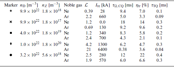
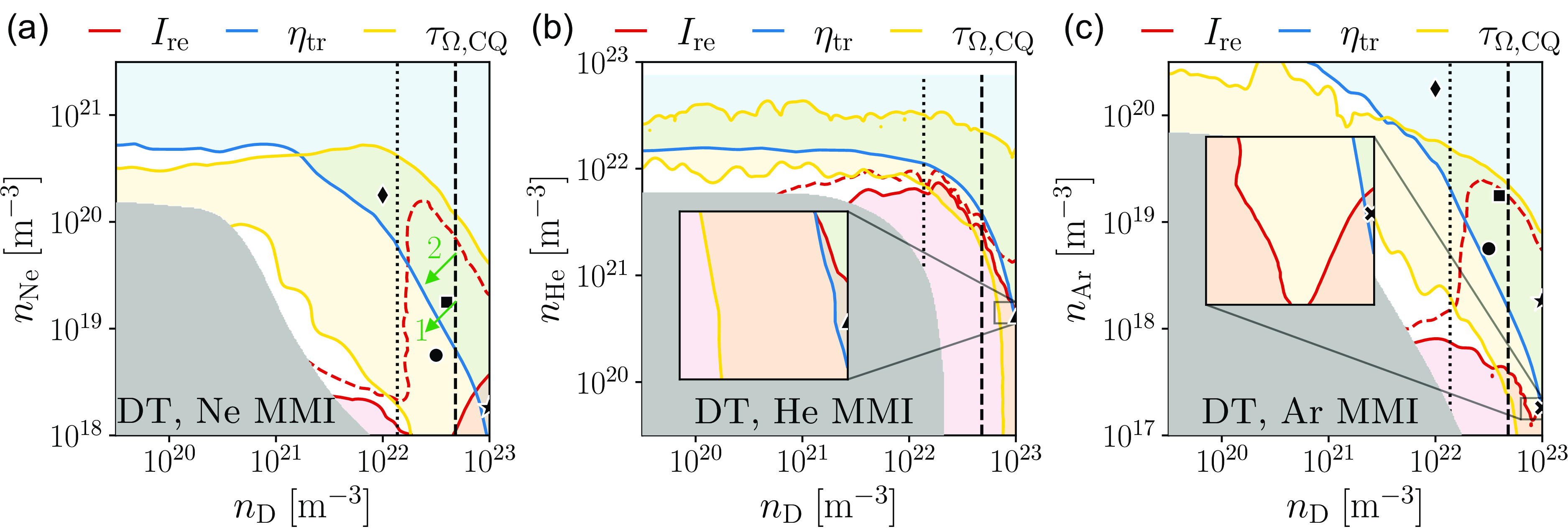
Figure 4. Regions of safe operation (shaded) with regards to $I_{\textrm {re}}$
(red),
$I_{\textrm {re}}$
(red), $\eta _{\textrm {tr}}$
(blue) and
$\eta _{\textrm {tr}}$
(blue) and $\tau _{\Omega ,\textrm {CQ}}$
(yellow) for DT operation with MMI of (a) Ne, (b) He and (c) Ar. Additionally, the red dashed line indicates where the runaway current is 1 MA, bounding the tolerable region of operation. The markers indicate the cases in table 3, while the optimal sample is indicated by a star in panel (a), a triangle in panel (b) and a cross in panel (c). The upper design limit of the D density during MGI in SPARC is indicated by the dashed vertical line for 44 % assimilation (
$\tau _{\Omega ,\textrm {CQ}}$
(yellow) for DT operation with MMI of (a) Ne, (b) He and (c) Ar. Additionally, the red dashed line indicates where the runaway current is 1 MA, bounding the tolerable region of operation. The markers indicate the cases in table 3, while the optimal sample is indicated by a star in panel (a), a triangle in panel (b) and a cross in panel (c). The upper design limit of the D density during MGI in SPARC is indicated by the dashed vertical line for 44 % assimilation ( ${n_{\textrm {D}}}={4.8\times 10^{22}}\, {\textrm {m}^{-3}}$
) and the dotted vertical line for 10 % assimilation. If the assimilation is lower than 44 %, the expected outcome of experiments using MMI densities along the line indicating 44 % would be shifted in the direction of the green arrows. The grey area covers the region of incomplete TQ.
${n_{\textrm {D}}}={4.8\times 10^{22}}\, {\textrm {m}^{-3}}$
) and the dotted vertical line for 10 % assimilation. If the assimilation is lower than 44 %, the expected outcome of experiments using MMI densities along the line indicating 44 % would be shifted in the direction of the green arrows. The grey area covers the region of incomplete TQ.
If we consider a relaxed tolerance limit of 1 MA for the runaway current, instead of 150 kA, we find that then there exists a region of tolerable disruptions, which is similar to the region of successful mitigation found during the optimisations of D operation, both with and without the Compton source. As the Compton scattering plays a larger role in the RE dynamics, the region of safe operation shrinks and this is mainly due to the reduced region of tolerable RE currents. This trend is clear when comparing figures 3(a) (D without Compton generation), figure 3(b) (D with DD-induced Compton generation) and figure 4(a) (DT with DT-induced Compton scattering). It is probable that for DT without any RE generation from Compton scattering, the corresponding optimisation landscape would look similar to that of a pure D plasma, illustrated in figure 2(a). Simulations of the samples of table 3 for a DT plasma (with MMI of Ne) without RE generation from Compton scattering further support this claim. Thus, experiments during D operation could help inform mitigation strategies during DT operation as well. Furthermore, using 1 MA as an upper safety limit for the cost function instead, the optimal sample would be located at ${n_{\textrm {D}}}\approx {4\times 10^{22}}\, { \textrm {m}^{-3}}$
and
${n_{\textrm {D}}}\approx {4\times 10^{22}}\, { \textrm {m}^{-3}}$
and ${n_{\textrm {Ne}}}\approx {2\times 10^{19}}\, {\textrm {m}^{-3}}$
, indicated by a square in figure 4(a), which is below the upper design limit of the D density at 44 % assimilation and thus would be easier to achieve under the MGI design constraints. For these D and Ne densities, we get a runaway current of 300 kA, which is still significantly smaller than 1 MA, and transported heat fraction of 6 %.
${n_{\textrm {Ne}}}\approx {2\times 10^{19}}\, {\textrm {m}^{-3}}$
, indicated by a square in figure 4(a), which is below the upper design limit of the D density at 44 % assimilation and thus would be easier to achieve under the MGI design constraints. For these D and Ne densities, we get a runaway current of 300 kA, which is still significantly smaller than 1 MA, and transported heat fraction of 6 %.
One important aspect to consider for this optimisation is how the uncertainty with regards to assimilation will affect the disruption mitigation. As assimilation is not known with certainty, it may be beneficial to choose injected quantities that may nominally perform somewhat poorer than the optimum, but are more robust with respect to such uncertainties. Currently, we have assumed a uniform distribution of the injected material, corresponding to 44 % assimilation. If the assimilation is ${\lt} {44}$
%, the densities of the injected material inside the plasma are lower, corresponding to (
${\lt} {44}$
%, the densities of the injected material inside the plasma are lower, corresponding to ( $n_{\textrm {D}}$
,
$n_{\textrm {D}}$
, $n_{\textrm {Ne}}$
) points being shifted in the direction indicated by the arrows in figure 4(a). Choosing Ne density to match what is predicted to be optimal (assuming
$n_{\textrm {Ne}}$
) points being shifted in the direction indicated by the arrows in figure 4(a). Choosing Ne density to match what is predicted to be optimal (assuming $I_{\textrm {re}}\lt {1}\, \textrm {MA}$
is acceptable), it is possible that the actual point in (
$I_{\textrm {re}}\lt {1}\, \textrm {MA}$
is acceptable), it is possible that the actual point in ( $n_{\textrm {D}}$
,
$n_{\textrm {D}}$
, $n_{\textrm {Ne}}$
) space would be shifted past the boundary of
$n_{\textrm {Ne}}$
) space would be shifted past the boundary of ${\eta _{\textrm {tr}}}={10}$
%, as indicated by the arrow labelled 1 in the figure, resulting in inadequate heat load mitigation. Figure 4(a) suggest that starting at a higher Ne density than what is predicted to optimal, sufficient mitigation of both the RE current and the transported fraction of the heat losses would be possible, even if the assimilation is less than 44 %, as indicated by the arrow labelled 2 in the figure.
${\eta _{\textrm {tr}}}={10}$
%, as indicated by the arrow labelled 1 in the figure, resulting in inadequate heat load mitigation. Figure 4(a) suggest that starting at a higher Ne density than what is predicted to optimal, sufficient mitigation of both the RE current and the transported fraction of the heat losses would be possible, even if the assimilation is less than 44 %, as indicated by the arrow labelled 2 in the figure.
How the runaway current, transported heat loss and CQ time relate to one another for each optimisation sample is illustrated in figure 5. The most interesting feature of this plot is that it shows the trade-off between each pair out of the three figures of merit. Figure 5(a) shows that for runaway currents lower than 150 kA, the transported heat loss will be larger than 5 %. The trade-off between having a small runaway current and transported heat fraction is a consequence of two attributes of the injected Ne. The purpose of injecting Ne, or another noble gas, for mitigating a disruption is to increase the heat being radiated from the plasma and thus reduce the amount of heat that is being transported to the wall. However, since Ne has $Z=10$
, this also means that more electrons are also added to the plasma, which will increase runaway current through enhanced avalanching, as
$Z=10$
, this also means that more electrons are also added to the plasma, which will increase runaway current through enhanced avalanching, as $\varGamma _{\textrm {ava}}\propto n_{\textrm {e, tot}}$
(where
$\varGamma _{\textrm {ava}}\propto n_{\textrm {e, tot}}$
(where $n_{\textrm {e, tot}}$
is the total electron density in the plasma). Thus, moving to the right along the Pareto frontFootnote
2
of the cloud in figure 5(a) corresponds to increasing the Ne density – the runaway current increases while the transported heat loss decreases.
$n_{\textrm {e, tot}}$
is the total electron density in the plasma). Thus, moving to the right along the Pareto frontFootnote
2
of the cloud in figure 5(a) corresponds to increasing the Ne density – the runaway current increases while the transported heat loss decreases.
The trade-off between the CQ time and the two other figures of merit is better, as most samples are within the safe interval for the CQ time. Notably, the safe (blue) samples are clustered around 10 ms, which is a favourable value that balances the concerns of eddy current and halo current forces. There are some samples with ${\tau _{\Omega ,\textrm {CQ}}}\lt {3.2}\, \textrm {ms}$
, which is lower than the SPARC components have been designed to withstand. In these Dream simulations, the full plasma current is almost completely converted into runaway current in less than 3.2 ms, and the total plasma current does therefore not decay significantly. Aside from the large runaway current, as indicated by figure 5(b), these samples have low values of the transported heat loss, as indicated by figure 5(c), signifying that they correspond to high Ne densities.
${\tau _{\Omega ,\textrm {CQ}}}\lt {3.2}\, \textrm {ms}$
, which is lower than the SPARC components have been designed to withstand. In these Dream simulations, the full plasma current is almost completely converted into runaway current in less than 3.2 ms, and the total plasma current does therefore not decay significantly. Aside from the large runaway current, as indicated by figure 5(b), these samples have low values of the transported heat loss, as indicated by figure 5(c), signifying that they correspond to high Ne densities.
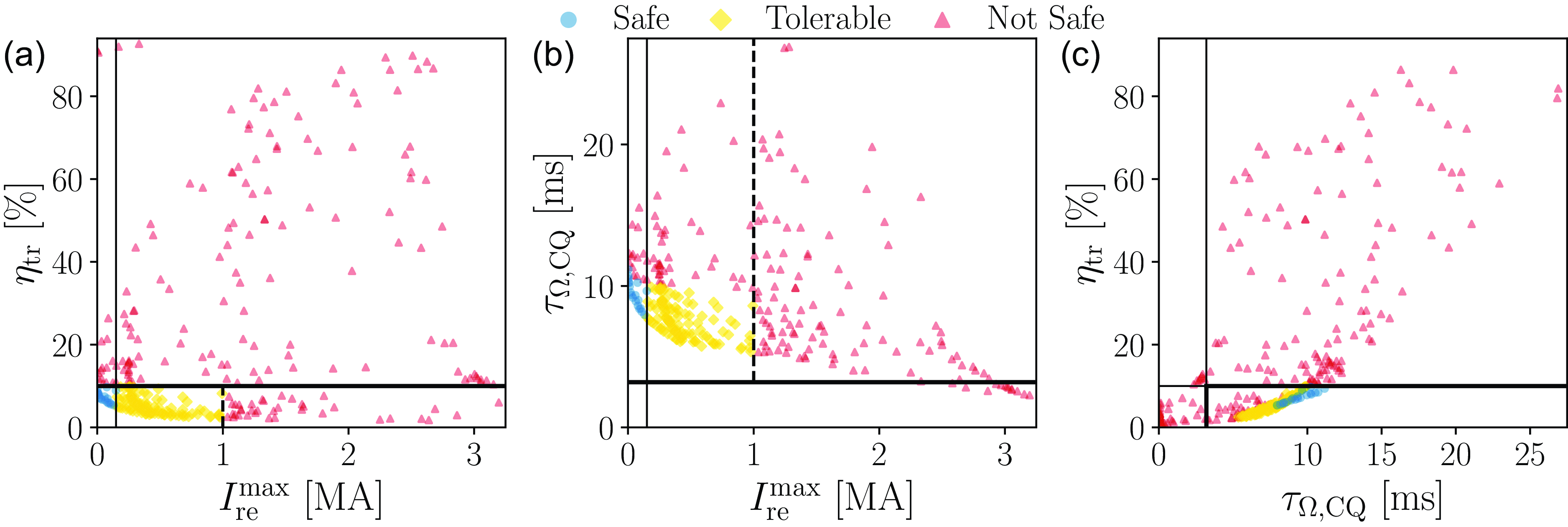
Figure 5. Projections of the simulation dataset to all the two-dimensional subspaces of the figure of merit space $(I_{\textrm {re}}, {\eta _{\textrm {tr}}}, {\tau _{\Omega ,\textrm {CQ}}})$
from the Ne MMI optimisation. The intervals of safe operation for each cost function component (see table 2 for the values) are indicated by the solid black lines, while the dashed black line indicates the potentially tolerable upper bound of the runaway current at 1 MA. Safe simulation samples are plotted in blue, tolerable samples (namely simulations with
$(I_{\textrm {re}}, {\eta _{\textrm {tr}}}, {\tau _{\Omega ,\textrm {CQ}}})$
from the Ne MMI optimisation. The intervals of safe operation for each cost function component (see table 2 for the values) are indicated by the solid black lines, while the dashed black line indicates the potentially tolerable upper bound of the runaway current at 1 MA. Safe simulation samples are plotted in blue, tolerable samples (namely simulations with $I_{\textrm {re}}\lt {1}\, \textrm {MA}$
and otherwise safe) are plotted in yellow and unsafe samples are plotted in red. This figure illustrates the trade-off between the different cost function components.
$I_{\textrm {re}}\lt {1}\, \textrm {MA}$
and otherwise safe) are plotted in yellow and unsafe samples are plotted in red. This figure illustrates the trade-off between the different cost function components.
Compared with ITER, there is thus a much more favourable compromise between the runaway current and transported heat fraction. In the ITER study, it was found that, for activated disruption simulations with a runaway current lower than 4 MA, the transported heat loss would be larger than 75 % and vice versa. Considering a number of samples from the SPARC optimisation with ${n_{\textrm {D}}}\gt {10^{22}}\, {\, \textrm {m}^{-3}}$
and
${n_{\textrm {D}}}\gt {10^{22}}\, {\, \textrm {m}^{-3}}$
and ${n_{\textrm {Ne}}}\lt {2\times 10^{20}}\, {\, \textrm {m}^{-3}}$
, namely the samples of table 3, all of them present a more favourable compromise than this. This is also illustrated in figure 5, where many of the samples from the optimisation can be found to have relatively low values of both
${n_{\textrm {Ne}}}\lt {2\times 10^{20}}\, {\, \textrm {m}^{-3}}$
, namely the samples of table 3, all of them present a more favourable compromise than this. This is also illustrated in figure 5, where many of the samples from the optimisation can be found to have relatively low values of both $I_{\textrm {re}}$
and
$I_{\textrm {re}}$
and $\eta _{\textrm {tr}}$
, while also having
$\eta _{\textrm {tr}}$
, while also having $\tau _{\Omega ,\textrm {CQ}}$
within its acceptable range.
$\tau _{\Omega ,\textrm {CQ}}$
within its acceptable range.
The main explanation for the better trade-off in SPARC, compared with ITER, is the lower initial plasma current. In the SPARC primary reference discharge, the initial plasma current is 8.7 MA, or 60 % of the 15 MA current in the ITER H-mode scenario. More specifically, the avalanche multiplication is exponentially sensitive to the initial plasma current and thus the difference in initial plasma current is the reason the runaway current can be more successfully mitigated at higher Ne densities in SPARC, allowing for a more acceptable level of heat transport. If SPARC would have a 15 MA initial plasma current instead of 8.7 MA, the runaway current for the optimal scenario found during the optimisation is 2.5 MA instead, if we naively assume that the magnetic geometry is kept unchanged.
For other noble gases, the trade-off between minimising runaway current and transported heat loss will still be present, but how it manifests can be different. We have done the same disruption optimisations for He and Ar MMI as well, to see how the disruption mitigation evolves with increasing atomic number of the noble gas. Notably, there is only a sliver of overlap between the safe region of the runaway current and the transported heat fraction for both the He and the Ar MMI density space, as illustrated in figures 4(b) and 4(c). Using Ne should thus be more advantageous with regards to disruption mitigation compared with He or Ar, due to the much larger region of overlap shown in figure 4(a).
More detailed plots of the landscapes of the runaway current, transported heat loss and CQ time for each noble gas are presented in figure 9 in Appendix A, where the figure of merit dataset projections can also be found (figure 10). With He, there is not sufficient radiative heat loss, causing the region of safety for the transported heat fraction to appear at very high He densities ${n_{\textrm {He}}}\sim {10^{22}}\, {\, \textrm {m}^{-3}}$
, where high runaway current can no longer be mitigated. For Ar, however, the acceptable level of heat transport is achieved even at low Ar densities if the D density is high enough, but it is still enough to cause significant RE avalanching. There is, however, a fairly large region of overlap between the region of safety for the transported heat fraction and the region of tolerable runaway current (
${n_{\textrm {He}}}\sim {10^{22}}\, {\, \textrm {m}^{-3}}$
, where high runaway current can no longer be mitigated. For Ar, however, the acceptable level of heat transport is achieved even at low Ar densities if the D density is high enough, but it is still enough to cause significant RE avalanching. There is, however, a fairly large region of overlap between the region of safety for the transported heat fraction and the region of tolerable runaway current ( $I_{\textrm {re}}\lt {1}\, \textrm {MA}$
) for the Ar MMI, but not for the He MMI.
$I_{\textrm {re}}\lt {1}\, \textrm {MA}$
) for the Ar MMI, but not for the He MMI.
That runaway currents are larger and transported heat fractions lower for Ar compared with Ne at the same atomic densities is exemplified in table 3. For the transported heat fraction the difference is generally a factor ${\sim} 2{-}3$
, while for the runaway currents, the difference can range from a factor of
${\sim} 2{-}3$
, while for the runaway currents, the difference can range from a factor of ${\sim} 2$
to orders of magnitude. The runaway current evolution for sample one (star), three (square) and four (diamond) from the table is plotted in figure 6. For samples one and three, the runaway current evolution is similar for Ne and Ar MMI, even though the magnitudes are different. In both cases and for both noble gases, the runaway current peaks and then starts to decline.
${\sim} 2$
to orders of magnitude. The runaway current evolution for sample one (star), three (square) and four (diamond) from the table is plotted in figure 6. For samples one and three, the runaway current evolution is similar for Ne and Ar MMI, even though the magnitudes are different. In both cases and for both noble gases, the runaway current peaks and then starts to decline.
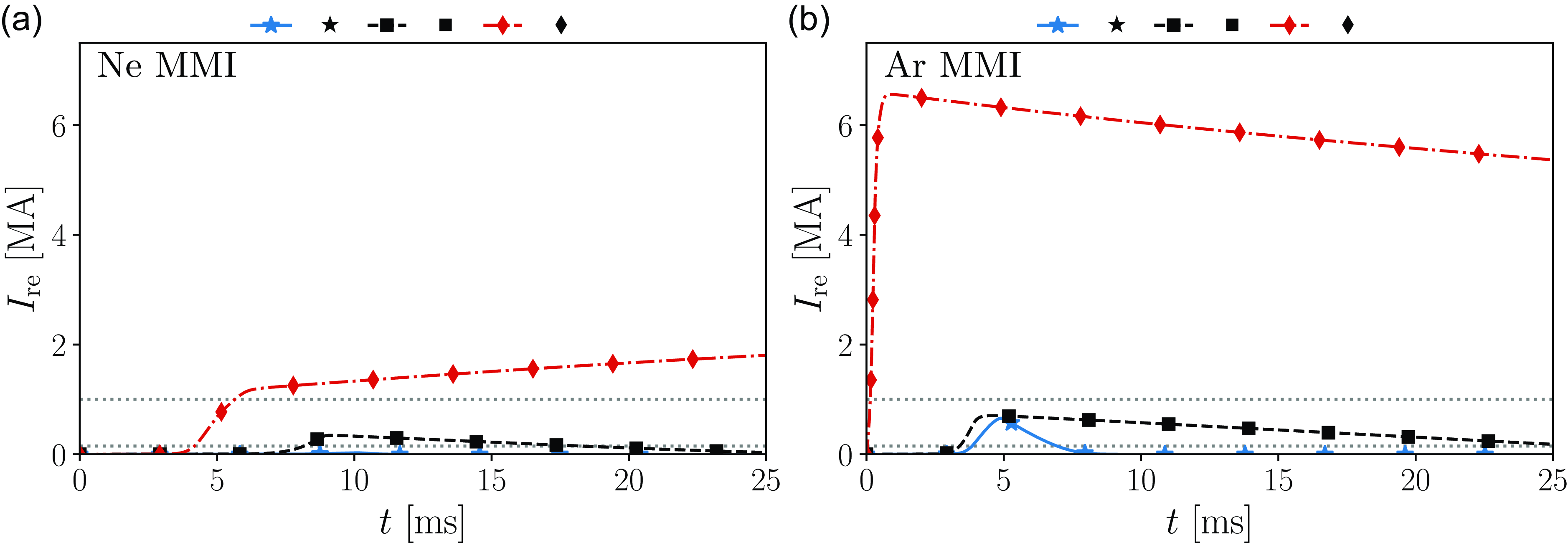
Figure 6. Current evolutions for the first (star, solid blue), third (square, dashed black) and fourth sample (diamond, dash-dotted red) of table 3 for (a) Ne and (b) Ar MMI. The grey dotted lines indicate $I_{\textrm {re}}={150}\, \textrm {kA}$
and
$I_{\textrm {re}}={150}\, \textrm {kA}$
and $I_{\textrm {re}}={1}\, \textrm {MA}$
.
$I_{\textrm {re}}={1}\, \textrm {MA}$
.
The runaway current dynamics is different for the fourth sample, however. With MMI of Ne, the RE generation is slower and it exceeds 150 kA after 3.4 ms, while with MMI of Ar, this happens already after 0.037 ms. For this Ar scenario, the RE generation is initially dominated by generation from momentum space flux, i.e. hot-tail and Dreicer generation, as illustrated in figure 7(b), but there is some generation from Compton scattering and tritium beta decay. After the TQ, the avalanche generation is dominant. Thus, for high amounts of injected, radiating impurities, there is significant RE seed formation from hot-tail and Dreicer generation, due to a fast temperature decay. In such a scenario, the REMC might not be effective in mitigating the RE current. The purpose of the REMC is to expel the RE seed before significant avalanching can occur or to at least have an RE loss rate that exceeds the growth rate. During a scenario with strong RE seed generation, it is possible that the RE primary generation rate is sufficiently high for a significant RE current to be produced by avalanching, despite the additional transport induced by the REMC.
It is possible to avoid large seeds from hot-tail and Dreicer generation, which for example is done in the third sample with MMI of Ne of table 3, as illustrated in figure 7(a). Here, there is no significant generation from hot-tail and Dreicer during the TQ, and no generation at all from tritium beta decay, indicated by the absence of a green curve in the figure, due to $p_{\textrm {c}}\gt p_{\textrm {max}}$
throughout the simulation, where
$p_{\textrm {c}}\gt p_{\textrm {max}}$
throughout the simulation, where $p_{\textrm {max}}$
is the maximum possible momentum for electrons emitted in beta decay. The generation from Compton scattering, however, is at approximately the same level as in figure 7(b), though for a longer period of time due to the longer duration of the TQ. The Compton scattering thus still generates a large enough RE seed that the runaway current, through avalanche generation, grows to 340 kA. Note that the short period of significant RE generation from flux through the upper boundary
$p_{\textrm {max}}$
is the maximum possible momentum for electrons emitted in beta decay. The generation from Compton scattering, however, is at approximately the same level as in figure 7(b), though for a longer period of time due to the longer duration of the TQ. The Compton scattering thus still generates a large enough RE seed that the runaway current, through avalanche generation, grows to 340 kA. Note that the short period of significant RE generation from flux through the upper boundary $p_{\textrm {re}}$
of the superthermal grid that happens after the TQ is still due to Compton generation. It is however delayed due to the time it takes for the REs generated at the end of the TQ with
$p_{\textrm {re}}$
of the superthermal grid that happens after the TQ is still due to Compton generation. It is however delayed due to the time it takes for the REs generated at the end of the TQ with $p_{\textrm {c}}\lt p\lt p_{\textrm {re}}$
to be accelerated to
$p_{\textrm {c}}\lt p\lt p_{\textrm {re}}$
to be accelerated to $p_{\textrm {re}}$
.
$p_{\textrm {re}}$
.
Importantly, the RE seed generated in the third sample of table 3 is mainly produced by the Compton scattering during the TQ. Using a reduction factor of $10^3$
, as was done by Vallhagen et al. (Reference Vallhagen, Hanebring, Artola, Lehnen, Nardon, Fülöp, Hoppe, Newton and Pusztai2024) and Ekmark et al. (Reference Ekmark, Hoppe, Fülöp, Jansson, Antonsson, Vallhagen and Pusztai2024), or
$10^3$
, as was done by Vallhagen et al. (Reference Vallhagen, Hanebring, Artola, Lehnen, Nardon, Fülöp, Hoppe, Newton and Pusztai2024) and Ekmark et al. (Reference Ekmark, Hoppe, Fülöp, Jansson, Antonsson, Vallhagen and Pusztai2024), or $10^2$
, instead of
$10^2$
, instead of $10^4$
only changes the maximum RE current by 10 kA or 90 kA, respectively. Neglecting the delayed photon flux altogether had no significant effect on the generated RE current. More generally, using a reduction factor of
$10^4$
only changes the maximum RE current by 10 kA or 90 kA, respectively. Neglecting the delayed photon flux altogether had no significant effect on the generated RE current. More generally, using a reduction factor of $10^3$
, the maximum runaway currents are at most increased by
$10^3$
, the maximum runaway currents are at most increased by ${\sim} {50}\, \textrm {kA}$
for the samples considered in table 3. Thus, for SPARC, the RE generation from delayed photon flux is not an important effect. However, since it is not possible to know this result a priori, accounting for a finite delayed photon flux is useful; indeed, the results of Vallhagen et al. (Reference Vallhagen, Hanebring, Artola, Lehnen, Nardon, Fülöp, Hoppe, Newton and Pusztai2024) indicate that the Compton seed created after the TQ losses may put a multi-MA lower bound on the RE currents in DT plasmas of ITER.
${\sim} {50}\, \textrm {kA}$
for the samples considered in table 3. Thus, for SPARC, the RE generation from delayed photon flux is not an important effect. However, since it is not possible to know this result a priori, accounting for a finite delayed photon flux is useful; indeed, the results of Vallhagen et al. (Reference Vallhagen, Hanebring, Artola, Lehnen, Nardon, Fülöp, Hoppe, Newton and Pusztai2024) indicate that the Compton seed created after the TQ losses may put a multi-MA lower bound on the RE currents in DT plasmas of ITER.
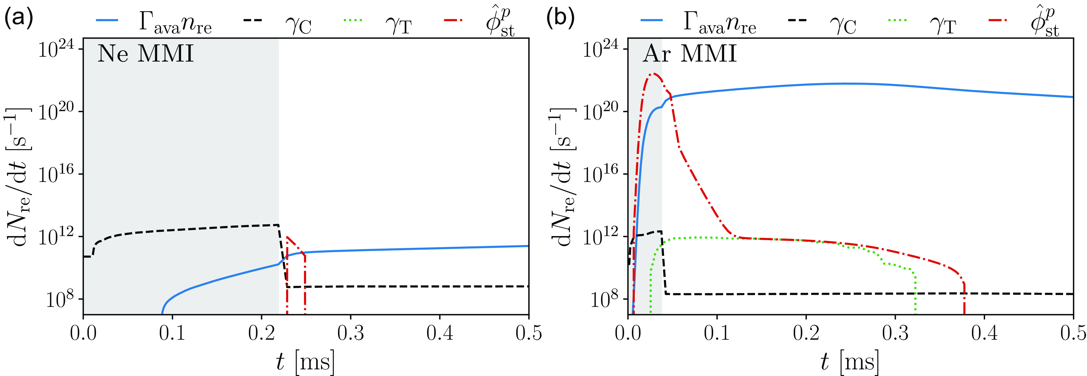
Figure 7. Volume integrated generation rates for (a) third sample (square) of table 3 using Ne as MMI material and (b) fourth sample (diamond) of table 3 using Ar as MMI material. The avalanche generation (denoted $\varGamma _{\textrm {ava}}{n_{\textrm {re}}}$
, note however that it is volume integrated) is plotted in solid blue, generation from Compton scattering (
$\varGamma _{\textrm {ava}}{n_{\textrm {re}}}$
, note however that it is volume integrated) is plotted in solid blue, generation from Compton scattering ( $\gamma _{\textrm {C}}=\int _{p\gt p_{\textrm {c}}}S_{\textrm {C}}\ \textrm {d}^3\boldsymbol{p}$
) in dashed black, generation from tritium beta decay (
$\gamma _{\textrm {C}}=\int _{p\gt p_{\textrm {c}}}S_{\textrm {C}}\ \textrm {d}^3\boldsymbol{p}$
) in dashed black, generation from tritium beta decay ( $\gamma _{\textrm {T}}=\int _{p\gt p_{\textrm {c}}}S_{\textrm {T}}\ \textrm {d}^3\boldsymbol{p}$
) in dotted green and the generation from flux across
$\gamma _{\textrm {T}}=\int _{p\gt p_{\textrm {c}}}S_{\textrm {T}}\ \textrm {d}^3\boldsymbol{p}$
) in dotted green and the generation from flux across $p_{\textrm {c}}$
(
$p_{\textrm {c}}$
( $\hat {\phi }_{\textrm {st}}^p =\phi _{\textrm {st}}^p-\int _{p_{\textrm {c}}}^{p_{\textrm {re}}}S_{\textrm {C}}+ S_{\textrm {T}}\ \textrm {d}^3\boldsymbol{p}$
) in dash-dotted red. The TQ phase is indicated by the grey shaded area.
$\hat {\phi }_{\textrm {st}}^p =\phi _{\textrm {st}}^p-\int _{p_{\textrm {c}}}^{p_{\textrm {re}}}S_{\textrm {C}}+ S_{\textrm {T}}\ \textrm {d}^3\boldsymbol{p}$
) in dash-dotted red. The TQ phase is indicated by the grey shaded area.
4. Conclusions
We have studied disruption mitigation in the primary reference discharge of SPARC using MMI of D and noble gases. We do so by optimising the MMI densities to find parameter regions with acceptably low levels of heat transport to the wall and runaway currents, as well as acceptable CQ durations. For the first time, we also consider the primary RE generation caused by Compton scattering in a tokamak activated by DD neutrons. We find that during D operation, disruptions can be successfully mitigated using MMI of D and Ne, even when accounting for the DD-induced Compton scattering. We observe, however, that this primary generation process does decrease the $n_{\textrm {D}}$
-
$n_{\textrm {D}}$
- $n_{\textrm {Ne}}$
parameter region corresponding to successful mitigation, signifying that generation from Compton scattering can play an important role even during D operation. Figures 2(a) and 2(b) display a possible path in parameter space that could be mapped out through D plasma experiments, i.e. performing several experiments with injected D and Ne densities chosen from the valley of the safe region of operation for a pure D plasma. This could give confidence in following the same trajectory in DT plasmas as well.
$n_{\textrm {Ne}}$
parameter region corresponding to successful mitigation, signifying that generation from Compton scattering can play an important role even during D operation. Figures 2(a) and 2(b) display a possible path in parameter space that could be mapped out through D plasma experiments, i.e. performing several experiments with injected D and Ne densities chosen from the valley of the safe region of operation for a pure D plasma. This could give confidence in following the same trajectory in DT plasmas as well.
For DT operation, we also find a region of successful mitigation with $I_{\textrm {re}}\lt {150}\, \textrm {kA}$
, but it requires D densities above the upper design limit of
$I_{\textrm {re}}\lt {150}\, \textrm {kA}$
, but it requires D densities above the upper design limit of ${n_{\textrm {D}}}={4.8\times 10^{22}}\, {\, \textrm {m}^{-3}}$
assuming 44 % assimilation. It is however possible to achieve tolerable disruptions, with
${n_{\textrm {D}}}={4.8\times 10^{22}}\, {\, \textrm {m}^{-3}}$
assuming 44 % assimilation. It is however possible to achieve tolerable disruptions, with $I_{\textrm {re}}\lt {1}\, \textrm {MA}$
, below this upper design limit. We thus find a more favourable compromise for acceptable values of the runaway current and transported heat fraction in SPARC compared with ITER, as in ITER, it was not possible to achieve
$I_{\textrm {re}}\lt {1}\, \textrm {MA}$
, below this upper design limit. We thus find a more favourable compromise for acceptable values of the runaway current and transported heat fraction in SPARC compared with ITER, as in ITER, it was not possible to achieve $I_{\textrm {re}}\lt {4}\, \textrm {MA}$
and
$I_{\textrm {re}}\lt {4}\, \textrm {MA}$
and ${\eta _{\textrm {tr}}}\lt {75}$
% simultaneously (Ekmark et al. Reference Ekmark, Hoppe, Fülöp, Jansson, Antonsson, Vallhagen and Pusztai2024). The main reason for the more favourable mitigation in SPARC is the lower initial plasma current, leading to lower avalanching.
${\eta _{\textrm {tr}}}\lt {75}$
% simultaneously (Ekmark et al. Reference Ekmark, Hoppe, Fülöp, Jansson, Antonsson, Vallhagen and Pusztai2024). The main reason for the more favourable mitigation in SPARC is the lower initial plasma current, leading to lower avalanching.
For DT operation, we also studied MMI of He and Ar in addition to Ne, but out of the three, Ne demonstrated the best trade-off between runaway current and transported heat. Out of He and Ar, Ar resulted in better mitigation, as the region for tolerable runaway currents ( $I_{\textrm {re}}\lt {1}\, \textrm {MA}$
) was significantly larger for Ar than for He. However, the region of tolerable runaway currents was larger still for Ne, compared with Ar, and there was a larger region of overlap between safe values of the runaway current (
$I_{\textrm {re}}\lt {1}\, \textrm {MA}$
) was significantly larger for Ar than for He. However, the region of tolerable runaway currents was larger still for Ne, compared with Ar, and there was a larger region of overlap between safe values of the runaway current ( $I_{\textrm {re}}\lt {150}\, \textrm {kA}$
) and the transported heat loss (
$I_{\textrm {re}}\lt {150}\, \textrm {kA}$
) and the transported heat loss ( ${\eta _{\textrm {tr}}}\lt {10}$
%). These results specifically regard single material injection for RE avoidance. According to recent work by Hollmann et al. (Reference Hollmann2023), for a double injection scheme, using Ar instead of Ne during the initial injection could be more beneficial for benign termination. However, recent work by Sheikh et al. (Reference Sheikh2024) and Hoppe et al. (Reference Hoppe2025) suggests that above a vessel pressure of 1 Pa, benign termination may no longer be effective, corresponding to a relatively low post-injection plasma D density of
${\eta _{\textrm {tr}}}\lt {10}$
%). These results specifically regard single material injection for RE avoidance. According to recent work by Hollmann et al. (Reference Hollmann2023), for a double injection scheme, using Ar instead of Ne during the initial injection could be more beneficial for benign termination. However, recent work by Sheikh et al. (Reference Sheikh2024) and Hoppe et al. (Reference Hoppe2025) suggests that above a vessel pressure of 1 Pa, benign termination may no longer be effective, corresponding to a relatively low post-injection plasma D density of ${6\times 10^{20}}\, {\, \textrm {m}^{-3}}$
in SPARC, which would greatly constrain the parameter space studied herein. Further the simulation work by Hollmann et al. suggests that the high current density in SPARC also challenges benign termination. As such, optimising the primary injection together with the REMC might be preferable.
${6\times 10^{20}}\, {\, \textrm {m}^{-3}}$
in SPARC, which would greatly constrain the parameter space studied herein. Further the simulation work by Hollmann et al. suggests that the high current density in SPARC also challenges benign termination. As such, optimising the primary injection together with the REMC might be preferable.
One point of note for the disruption simulations in this work is the relatively simple MMI model used. In the model, the material is instantly and uniformly distributed in the plasma, and the transport due to magnetic field line stochastisation is activated simultaneously. In reality, the material would require time to penetrate the plasma from the edge, which could significantly impact the plasma evolution and runaway electron dynamics. Accounting for a more realistic model of the injected material deposition, with temporal and spatial variations, would mean that plasma cooling would happen earlier farther out from the magnetic axis. This could trigger magnetic perturbations in the core before the material has penetrated that far into the plasma. Notably, this would impact runaway dynamics through transport, the hot-tail generation – as the cooling dynamics could be significantly different –, as well as the other seed generation mechanisms – as the evolution of the critical and Dreicer fields could be affected. More specifically, the hot-tail generation could be overestimated by our model, due to the drastic temperature decay in the core caused by instantaneous deposition. However, the mitigating effects of the injected material could also be overestimated for the same reason. Assessing these effects would require self-consistent modelling of the material penetration, MHD instabilities and runaway dynamics, and is outside the scope of the paper. It is however worth pointing out that the pre-TQ duration is estimated to be ${\sim} {2}\, \textrm {ms}$
according to the ITPA Disruption Database (Eidietis et al. Reference Eidietis2015), and the disruption mitigation system currently under construction for SPARC should be able to deliver a D density of
${\sim} {2}\, \textrm {ms}$
according to the ITPA Disruption Database (Eidietis et al. Reference Eidietis2015), and the disruption mitigation system currently under construction for SPARC should be able to deliver a D density of ${4.4\times 10^{22}}\, {\, \textrm {m}^{-3}}$
during this time. Thus, for pure D operation, the densities required for successful mitigation are attainable during the pre-TQ with the current system. For DT plasmas, the densities required could be reached, but the fuel processing systems may constrain the maximum allowable injection.
${4.4\times 10^{22}}\, {\, \textrm {m}^{-3}}$
during this time. Thus, for pure D operation, the densities required for successful mitigation are attainable during the pre-TQ with the current system. For DT plasmas, the densities required could be reached, but the fuel processing systems may constrain the maximum allowable injection.
In this study, we have not accounted for other relevant effects that could help mitigate the disruptions, such as plasma scrape-off (Wang et al. Reference Wang, Nardon, Artola, Bandaru and Hoelzl2024; Vallhagen et al. Reference Vallhagen, Hanebring, Fülöp, Hoppe, Votta and Pusztai2025), secondary material injection into a developed RE beam (Paz-Soldan et al. Reference Paz-Soldan, Eidietis, Liu, Shiraki, Boozer, Hollmann, Kim and Lvovskiy2019; Reux et al. Reference Reux2021) and the use of an REMC (Tinguely et al. Reference Tinguely2021). Previous studies suggest that these effects can drastically limit the impact or size of the runaway current. This means that the runaway currents found in this study represent a worst-case scenario for what could happen during a disruption in SPARC. Other effects which we have neglected that could change the figure of merit landscape are the impurity deposition profile and its time evolution, impurity injection duration, equilibrium evolution and RE ionisation.
In summary, we find that acceptable levels of runaway current and transported heat losses can be achieved in D operation, even without the REMC. This applies also to DT plasmas if the injected D densities can be increased above the nominal upper limit for the SPARC MGI system or assimilation closer to 70 % (corresponding to ${n_{\textrm {D}}}={10^{23}}\, {\, \textrm {m}^{-3}}$
) can be achieved. Considering how massive material injection can expand the safe mitigation space when used in combination with the REMC, and how it might be used to relax requirements on the mitigation coil system, appear as interesting avenues for future investigation.
${n_{\textrm {D}}}={10^{23}}\, {\, \textrm {m}^{-3}}$
) can be achieved. Considering how massive material injection can expand the safe mitigation space when used in combination with the REMC, and how it might be used to relax requirements on the mitigation coil system, appear as interesting avenues for future investigation.
Acknowledgements
The authors are grateful to O. Vallhagen, E. Nardon and S. Newton for fruitful discussions and to H. Boyd for providing the MCNP data.
Editor Per Helander thanks the referees for their advice in evaluating this article.
Funding
This work was supported by the Swedish Research Council (Dnr. 2022-02862 and 2021-03943), and by the Knut and Alice Wallenberg foundation (Dnr. 2022.0087 and 2023.0249). The work has been carried out within the framework of the EUROfusion Consortium, funded by the European Union via the Euratom Research and Training Programme (Grant Agreement No 101052200 – EUROfusion). Views and opinions expressed are however those of the authors only and do not necessarily reflect those of the European Union or the European Commission. Neither the European Union nor the European Commission can be held responsible for them. R.A.T. and R.S. are supported by Commonwealth Fusion Systems.
Declaration of interests
The authors report no conflict of interest.
Appendix A. Figure of merit landscapes and trade-off
Here, we present more detailed plots of the figure of merit landscapes in the injected density parameter space. In figure 8, the figure of merit landscapes obtained from the optimisation of D operation are presented, both with (figure 8 b) and without (figure 8 a) RE generation from DD-induced Compton scattering. The figure of merit landscapes obtained from the optimisation of DT operation are presented in figure 9, for MMI of Ne (figure 9 a), He (figure 9 b) and Ar (figure 9 c).

Figure 8. Logarithmic contour plots of the figure of merit estimates from the optimisations of D operation (a) without and (b) with RE generation from DD-induced Compton scattering.
The trade-off among the runaway current, transported fraction of the heat loss and CQ time for the optimisation dataset from DT operation with MMI of He and Ar are plotted in figures 10(a) and 10(b), respectively.
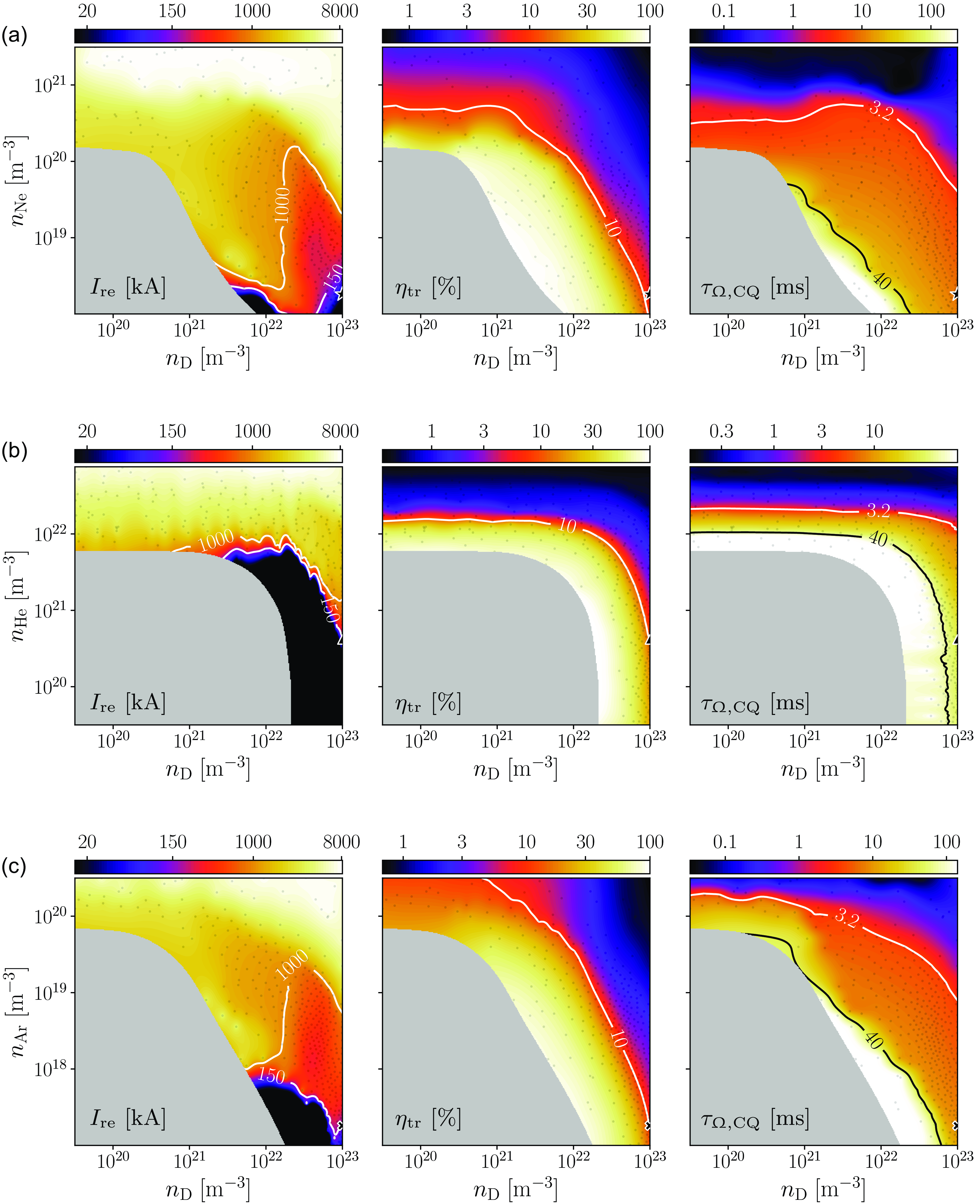
Figure 9. Logarithmic contour plots of the figure of merit estimates from the optimisations of DT operation with MMI of D in combination with (a) Ne, (b) He and (c) Ar.
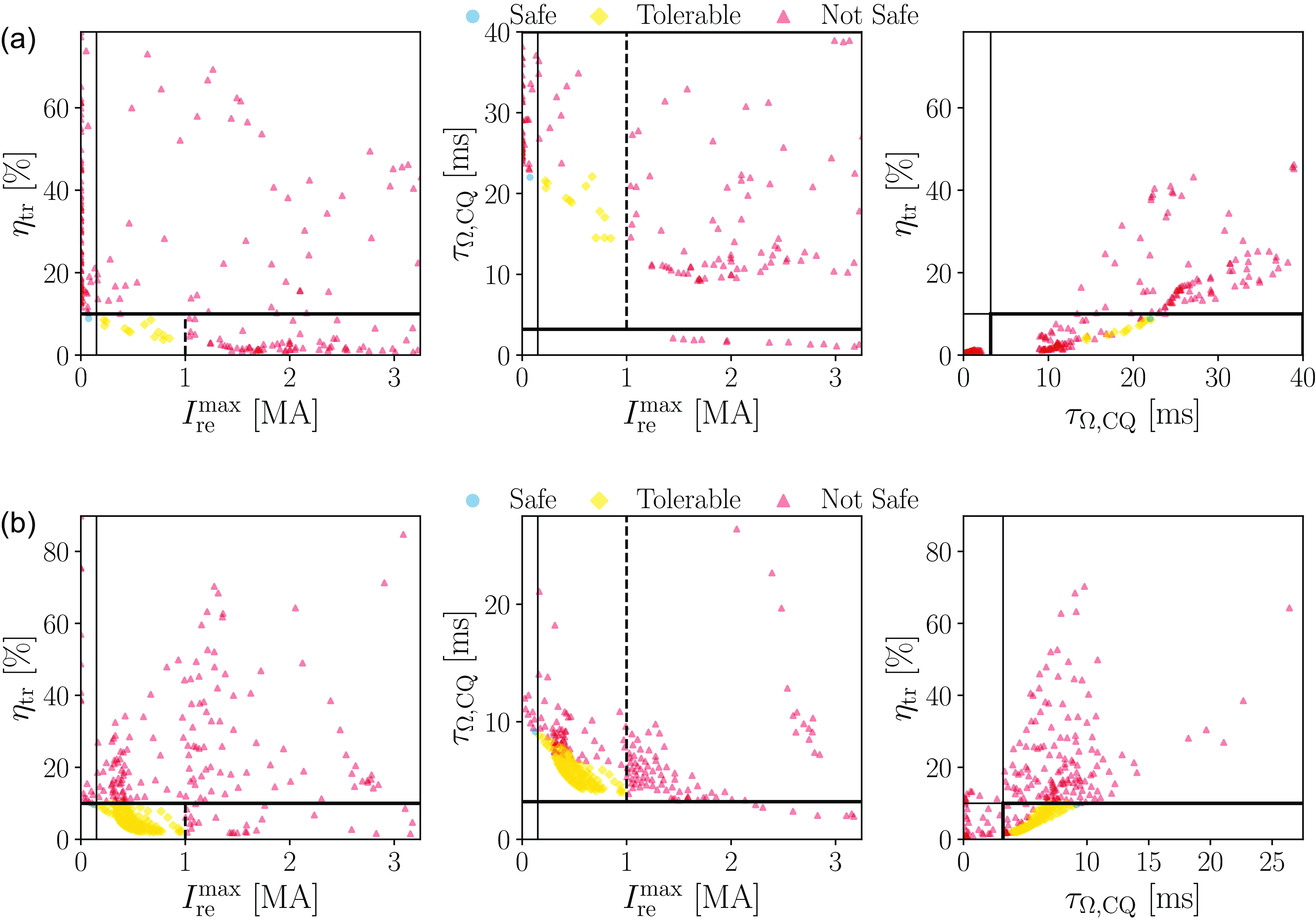
Figure 10. Projections of the simulation dataset to all the two-dimensional subspaces of the figure of merit space $(I_{\textrm {re}}, {\eta _{\textrm {tr}}}, {\tau _{\Omega ,\textrm {CQ}}})$
from the (a) He and (b) Ar MMI optimisation.
$(I_{\textrm {re}}, {\eta _{\textrm {tr}}}, {\tau _{\Omega ,\textrm {CQ}}})$
from the (a) He and (b) Ar MMI optimisation.


 Open access