1. Introduction
The increasing frequency and intensity of extreme weather events associated with global climate change has raised widespread concern in both practice and academia. As highlighted by the Sixth Assessment Report (AR6) of the Intergovernmental Panel on Climate Change, the number of record-breaking extreme precipitation events globally has significantly increased over the past decades, with a faster rate since 1980. In 2024, disaster events related to extreme precipitation, such as floods and landslides, have affected at least four continents, including regions in Central Asia, West and East Africa, Central Europe, and the southern United States with thousands of people displaced and millions losing access to basic infrastructure. The occurrences draw attention to the detrimental impacts associated with extreme precipitation events, which are projected to become unprecedentedly more frequent and intense in the future.
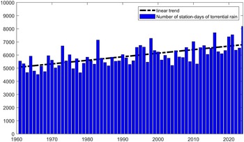
Prompted by the growing concern over the widespread adverse effects of severe rainfall, we aim to investigate the impacts of extreme precipitation on corporate leverage in the context of China. China presents an ideal setting for this investigation for several compelling reasons. China remains one of the most precipitation-affected regions globally. As shown in Figure 1, the annual station-days of torrential rain in China have increased significantly in the past several decades. In 2024, the total station-days of torrential rain across China (sum of torrential rain days recorded by all meteorological stations) reached 8,186 station-days, which is 32% higher than the annual average between 1960 and 2024. According to the Ministry of Emergency Management in China, natural disasters across China in the first half of 2025 brought direct economic losses of 54.11 billion yuan, of which heavy rainfall and flooding caused the most damage, accounting for over 90% of this year’s total losses at 51 billion yuan. Meanwhile, as the world’s second-largest economy with a state-dominated financial system, China’s corporate leverage ratio is now among the highest globally, having risen nearly 65 percentage points within a decade, making it highly exposed to weather-related disaster risk. This high leverage in the corporate sector might make firms susceptible to weather-related disasters, and motivates us to examine the impacts of extreme rainfall on real economy from the perspective of firm’s leverage dynamics.
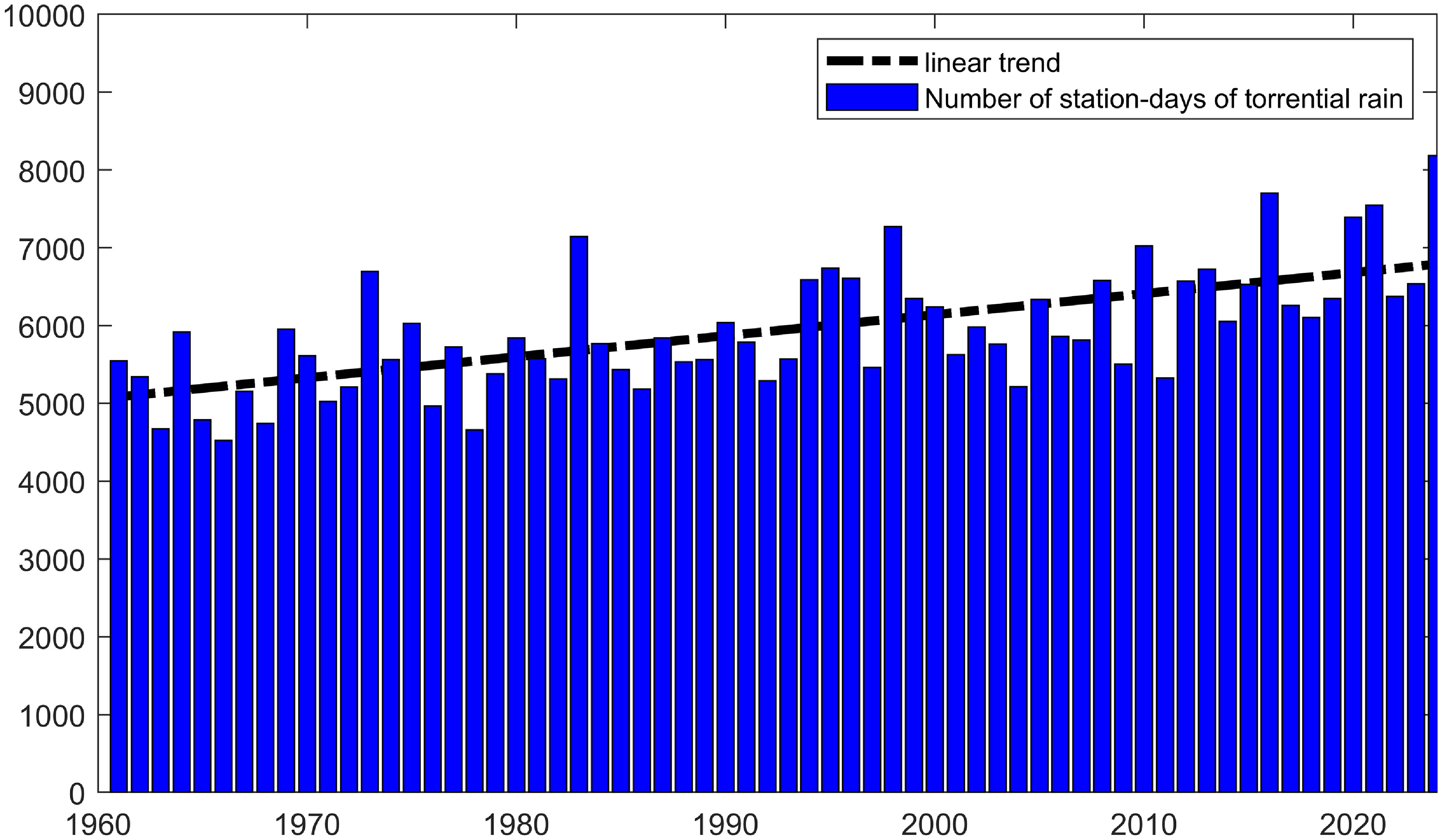
Figure 1. Number of station-days of torrential rain in China (1960–2024).
We construct a province-level extreme rainfall series
 $ExtRain$
based on grid-based meteorological datasets, and quantify the impacts of extreme precipitation on corporate leverage using firm-level regression from 2010 to 2023. We identify two channels through which extreme precipitation affects firm’s leverage: the firm’s balance sheet channel and the local government’s crowding-out channel. Given these empirical results, we further develop a New Keynesian DSGE model with extreme rainfall shock (ERS) and Chinese characteristics, to explain the transmission mechanism from extreme precipitation to firm sector. Based on the model, we further quantify the welfare cost and mitigation policies associated with ERS. Our baseline findings reveal that the intense rainfall would bring about a significant decline in firm’s leverage. The channel tests indicate that severe rainfall adversely affects firm’s leverage by depressing its balance sheet and intensifying local government’s crowding-out effects. Moreover, the simulations from the new Keynesian DSGE model featuring ERS and China’s land finance system corroborate our empirical findings. The welfare analysis show that the welfare cost caused by extreme rainfall risk can amount to 2.2% of the agent’s lifetime utility, and accommodative monetary policy and active fiscal policy could be utilized to alleviate the adverse impacts of ERS.
$ExtRain$
based on grid-based meteorological datasets, and quantify the impacts of extreme precipitation on corporate leverage using firm-level regression from 2010 to 2023. We identify two channels through which extreme precipitation affects firm’s leverage: the firm’s balance sheet channel and the local government’s crowding-out channel. Given these empirical results, we further develop a New Keynesian DSGE model with extreme rainfall shock (ERS) and Chinese characteristics, to explain the transmission mechanism from extreme precipitation to firm sector. Based on the model, we further quantify the welfare cost and mitigation policies associated with ERS. Our baseline findings reveal that the intense rainfall would bring about a significant decline in firm’s leverage. The channel tests indicate that severe rainfall adversely affects firm’s leverage by depressing its balance sheet and intensifying local government’s crowding-out effects. Moreover, the simulations from the new Keynesian DSGE model featuring ERS and China’s land finance system corroborate our empirical findings. The welfare analysis show that the welfare cost caused by extreme rainfall risk can amount to 2.2% of the agent’s lifetime utility, and accommodative monetary policy and active fiscal policy could be utilized to alleviate the adverse impacts of ERS.
Our research is related to the literature on the economic impacts of extreme weather events. Previous research has documented the substantial negative effects of extreme weather events on various economic indicators, including economic growth, agricultural productivity, labor productivity, employment and social stability (Dell et al., Reference Dell, Jones and Olken2012; Hsiang et al., Reference Hsiang, Burke and Miguel2013; Burke et al., Reference Burke, Hsiang and Miguel2015). Although most of these studies focus on the detrimental effects of extreme temperatures and sea level rise, a number of studies have begun to consider the impacts of severe precipitation events on economic activities. To be specific, the ramifications of extreme precipitation, often occurring alongside droughts and floods (Davenport et al., Reference Davenport, Burke and Diffenbaugh2021), adversely affect economic growth both directly and indirectly through decreased agricultural productivity, infrastructure damage, and supply chain disruptions, etc. In contrast, several studies suggest that the impacts of precipitation changes on economic growth remain relatively insignificant (Barrios et al., Reference Barrios, Bertinelli and Strobl2010; Damania et al., Reference Damania, Desbureaux and Zaveri2020; Dell et al., Reference Dell, Jones and Olken2012; Kotz et al., Reference Kotz, Levermann and Wenz2022). Recent empirical evidence demonstrates that extreme precipitation events have significantly stronger negative effects on corporate financial outcomes compared to other weather-related shocks (Li et al., Reference Li, Chen and Yuan2025). This motivates us to examine the impacts of extreme rainfall on real economy from the perspective of firm’s leverage dynamics. Unlike most previous research relying on the reduced-form analysis of extreme weather events, we quantify the impacts of severe rainfall by combining panel regression and structural model simulations.
The present study also belongs to the emerging literature that assesses the firm-level implications of climate change. A number of researchers have postulated the negative influence of extreme weather and climate risks on vital aspects of firm performance, including productivity, total factor productivity (TFP), sales revenue, operating income, and operational costs (Zhang et al., Reference Zhang, Deschenes, Meng and Zhang2018; Chen and Yang, Reference Chen and Yang2019; Addoum et al., Reference Addoum, Ng and Ortiz-Bobea2020; Somanathan et al., Reference Somanathan, Somanathan, Sudarshan and Tewari2021; Addoum et al., Reference Addoum, Ng and Ortiz-Bobea2023; Pankratz et al., Reference Pankratz, Bauer and Derwall2023). Moreover, severe weather events have been linked to rising loan delinquency and mortgage default rates among firms (Aguilar-Gomez et al., Reference Aguilar-Gomez, Gutierrez, Heres, Jaume and Tobal2024; Calabrese et al., Reference Calabrese, Dombrowski, Mandel, Pace and Zanin2024). Additionally, Chen et al. (Reference Chen, Liu, Zhang and Zhang2023) and Rao et al. (Reference Rao, Koirala, Thapa and Neupane2022) highlight the significant impacts of extreme precipitation on firms’ investment and financing decisions. Although existing studies provide evidence of the adverse consequences associated with extreme weather events at the firm-level, research focusing on the impacts of extreme rainfall on corporate leverage is scarce, and we fill this gap by providing the specific mechanisms through which intense precipitation affects firm’s leverage.
This paper is also linked with the research on the impacts of extreme climate risk on government finance. Several studies have considered the effects of climate change on sovereign risk. Cevik and Jalles (Reference Cevik and Jalles2022) find that countries with greater climate resilience have been found to have lower bond yields and spreads. A number of authors have demonstrated that extreme heat and sea level rise will lead to a decline in economic output and an increase in government spending on post-disaster reconstruction, which would weaken the fiscal capacity and affect their fiscal balance of local governments, thereby increasing the risk of municipal bond defaults and refinancing (Lis and Nickel, Reference Lis and Nickel2010; Painter, Reference Painter2020). We complement this strand of literature by examining the role of China’s local government land finance system in propagating the ERS to corporate leverage.
Our research extends previous investigations in two aspects. First, we quantify the impacts of severe precipitation events on corporate leverage and analyze two mechanisms behind the impacts. The present study is closely related to Ginglinger and Moreau (Reference Ginglinger and Moreau2023), which investigate how climate risk affects firms’ financial leverage through higher expected distress costs and operating costs. We differ from them by emphasizing the role of China’s government financing in the propagation of extreme precipitation to corporate leverage.
Specifically, we are the first to investigate the effects of extreme weather events based on the perspective of China’s local governments’ land finance system, which is a key component of China’s economic development in the past decades. From 2007 to 2020, local governments in China have accumulated over 55 trillion yuan in land concessions, with land-related revenues reaching approximately 4 trillion yuan in 2018, accounting for over 40% of local fiscal revenues. Therefore, fluctuations in land prices emerge as a significant accelerator in the face of catastrophic events. Severe rainfall may generate downward pressure of land price, directly reduce land sale revenues, and heighten the debt pressure of local governments, which may spillover to enterprise and adversely affect credit resources to firm sector. This novel local government crowding-out channel triggered by extreme weather shock, which has not been explored in the existing literature, remains to be an important propagation mechanism in our analysis.
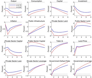
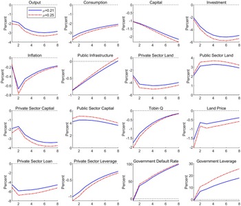
Secondly, we employ both reduced-form firm-level analysis and structural model simulations to explore the impacts of intense precipitation. We develop a New Keynesian DSGE model with ERS to uncover the mechanisms behind the empirical findings. Our DSGE model adds to the existing research on Hashimoto and Sudo (Reference Hashimoto and Sudo2024) by further incorporating firm’s credit constraints and China’s land finance system. Through the counterfactual impulse response analysis, we validate firm’s balance sheet channel and local government crowding-out channel, which is consistent with the empirical facts. Moreover, we study the welfare cost associated with ERS and examine the role of monetary and fiscal policy in mitigating the adverse impacts of ERS. These results have important policy implications for government climate adaptation strategy.
The remainder of this paper is organized as follows. Section 2 provides the empirical evidence about the effects of extreme rainfall on firm’s leverage. Section 3 builds a DSGE model with ERS to interpret our empirical findings. Section 4 concludes and outlooks.
2. Empirical evidence
2.1 Measuring extreme rainfall in China
To match the precipitation data with firm-level data, we pin down the exact location of each firm and employ the extreme rainfall in the province where the firms are located to identify the firm-level exposure to extreme precipitation events. To capture the province-level concentrated rainfall in China, we utilize the meteorological data set published by US National Centers for Environmental Information. To be specific, we focus on the grids-based (the resolution of 2.5 by 2.5 degrees latitude and longitude) weather data covering about 668 meteorological stations in mainland China. We extract the daily average precipitation of these stations within each grid. Armed with these grids-based daily precipitation values, we then define the variable
 $MaxRain_{i,m,y}$
as the maximum precipitation level in a 5-day window for location
$MaxRain_{i,m,y}$
as the maximum precipitation level in a 5-day window for location
 $i$
in month
$i$
in month
 $m$
and year
$m$
and year
 $y$
. To facilitate the aggregation of precipitation values across different locations, we convert
$y$
. To facilitate the aggregation of precipitation values across different locations, we convert
 $MaxRain_{i,m,y}$
into the standardized anomalies
$MaxRain_{i,m,y}$
into the standardized anomalies
 $MaxRain^{std}_{i,m,y}$
, by subtracting the mean value of
$MaxRain^{std}_{i,m,y}$
, by subtracting the mean value of
 $MaxRain_{i,m,y}$
and dividing the standard deviation of
$MaxRain_{i,m,y}$
and dividing the standard deviation of
 $MaxRain_{i,m,y}$
in the reference period. Thus, the standardized anomaly
$MaxRain_{i,m,y}$
in the reference period. Thus, the standardized anomaly
 $MaxRain_{i,m,y}$
measures the degree of deviation of the monthly precipitation value from the mean in the reference period for location
$MaxRain_{i,m,y}$
measures the degree of deviation of the monthly precipitation value from the mean in the reference period for location
 $i$
in month
$i$
in month
 $m$
and year
$m$
and year
 $y$
.
$y$
.
As our main data range is from 1990 to 2023, we take the first half (January 1990 to December 2005) as the reference period. For each month
 $m=1,2,$
…,
$m=1,2,$
…,
 $12$
and for each component variable
$12$
and for each component variable
 $MaxRain^{std}_{i,m,y}$
, we take the difference between
$MaxRain^{std}_{i,m,y}$
, we take the difference between
 $MaxRain^{std}_{i,m,y}$
and the mean of
$MaxRain^{std}_{i,m,y}$
and the mean of
 $MaxRain^{std}_{i,m,y}$
in month
$MaxRain^{std}_{i,m,y}$
in month
 $m$
of all years in the reference period, and scale the difference by the corresponding standard deviation of
$m$
of all years in the reference period, and scale the difference by the corresponding standard deviation of
 $MaxRain^{std}_{i,m,y}$
in the reference period.Footnote
1
Therefore, the standardized variables capture the severity and frequency of extreme rainfall events compared with the reference period. As we compute
$MaxRain^{std}_{i,m,y}$
in the reference period.Footnote
1
Therefore, the standardized variables capture the severity and frequency of extreme rainfall events compared with the reference period. As we compute
 $MaxRain^{std}_{i,m,y}$
month by month, the standardized variable naturally accounts for the seasonal precipitation patterns at the monthly frequency.
$MaxRain^{std}_{i,m,y}$
month by month, the standardized variable naturally accounts for the seasonal precipitation patterns at the monthly frequency.
In the last step of construction, the monthly sequences of standardized anomaly
 $MaxRain^{std}_{i,m,y}$
from different areas in mainland China are then averaged across the locations within each province. To align with quarterly firm-level observations, we transform the monthly anomaly into quarterly series by taking the simple average. This yields province-level extreme rainfall measure
$MaxRain^{std}_{i,m,y}$
from different areas in mainland China are then averaged across the locations within each province. To align with quarterly firm-level observations, we transform the monthly anomaly into quarterly series by taking the simple average. This yields province-level extreme rainfall measure
 $ExtRain_{j,t}$
for province
$ExtRain_{j,t}$
for province
 $j$
in quarter
$j$
in quarter
 $t$
.
$t$
.
2.2 Research design
We employ the following panel fixed effects model to examine the effect of severe rainfall on firm’s leverage:
 \begin{align} Lev_{i,j,t}&=\beta _0+\beta _1 ExtRain_{j,t}+\beta _2 X_{i,j,t-1}+\lambda _{t}+\mu _i+\epsilon _{i,j,t} , \end{align}
where the main dependent variable
 $Lev_{i,j,t}$
is the leverage of firm
$Lev_{i,j,t}$
is the leverage of firm
 $i$
located in province
$i$
located in province
 $j$
in quarter
$j$
in quarter
 $t$
.
$t$
.
 $ExtRain_{j,t}$
is the extreme rainfall series in province
$ExtRain_{j,t}$
is the extreme rainfall series in province
 $j$
, where the firm is located in quarter
$j$
, where the firm is located in quarter
 $t$
. The main parameter of interest is
$t$
. The main parameter of interest is
 $\beta _1$
, which reflects the marginal effects of extreme rainfall on firm’s leverage.
$\beta _1$
, which reflects the marginal effects of extreme rainfall on firm’s leverage.
 $\mu _i$
is firm-level fixed effect, while
$\mu _i$
is firm-level fixed effect, while
 $\lambda _{t}$
is year-quarter fixed effect.
$\lambda _{t}$
is year-quarter fixed effect.
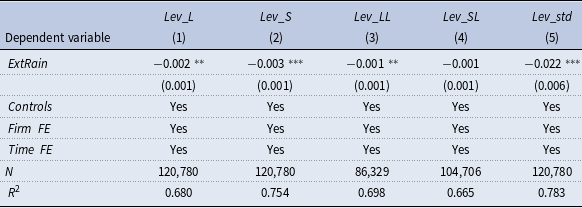
We use the ratio of firm’s total liabilities to total assets as the primary measure for firm’s leverage. We also employ several other proxies for corporate leverage in the robustness check, including the long-term (short-term) debt and non-current (current) liabilities scaled by total assets.
 $X_{i,j,t-1}$
is a series of control variables. We control for the following firm-level characteristics in our analyses: (1)
$X_{i,j,t-1}$
is a series of control variables. We control for the following firm-level characteristics in our analyses: (1)
 $ROA$
, return on total assets; (2)
$ROA$
, return on total assets; (2)
 $FixedAsset$
, the ratio of fixed assets to total assets; (3)
$FixedAsset$
, the ratio of fixed assets to total assets; (3)
 $EPS$
, earnings per outstanding share; (4)
$EPS$
, earnings per outstanding share; (4)
 $SOE$
, which equals to 1 for state-owned enterprise and 0 otherwise; (5)
$SOE$
, which equals to 1 for state-owned enterprise and 0 otherwise; (5)
 $LSH$
, the proportion of shares held by the largest shareholder. To control the time-variant provincial macroeconomic conditions and industrial structure, we include the logarithmic value of regional gross domestic product (
$LSH$
, the proportion of shares held by the largest shareholder. To control the time-variant provincial macroeconomic conditions and industrial structure, we include the logarithmic value of regional gross domestic product (
 $GDP$
) and logarithmic growth rate of employment in the secondary industry(
$GDP$
) and logarithmic growth rate of employment in the secondary industry(
 $Emp$
).
$Emp$
).
Our sample covers A-share listed companies from 2010Q1 to 2023Q3. We acquire firm-level observations from the CSMAR database, while regional macroeconomic data were sourced from the Economic Statistical Yearbook of provinces (2011–2023) and the CEIC database. We exclude firms within the financial and real estate industry, firms with the designation of “ST” and “PT,” and firms with fewer than five observations in the sample. Our eventual dataset includes an unbalanced panel of 150,839 “quarter-firm” observations from 4,518 companies. All the variable definitions and descriptive statistics are given in Appendix A.
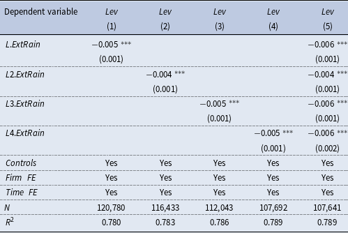
2.3 Baseline regressions
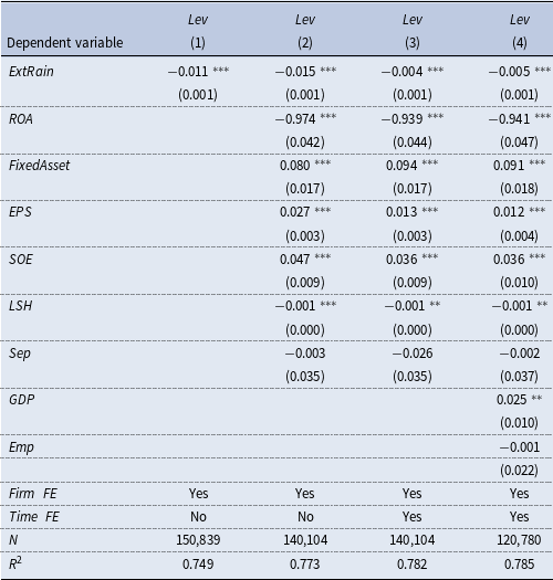
The baseline regression results are presented in Table 1. Column (1) does not include control variables, and the coefficient on
 $ExtRain$
is significantly negative, suggesting that an increase of extreme rainfall leads to the decrease of firm’s leverage. Column (2) controls for several firm-level characteristics, and the coefficient on
$ExtRain$
is significantly negative, suggesting that an increase of extreme rainfall leads to the decrease of firm’s leverage. Column (2) controls for several firm-level characteristics, and the coefficient on
 $ExtRain$
remains negatively significant at the 1% level. Column (3) adds the year-quarter fixed effects, while column (4) further includes province-level control variables, and the negative coefficient on
$ExtRain$
remains negatively significant at the 1% level. Column (3) adds the year-quarter fixed effects, while column (4) further includes province-level control variables, and the negative coefficient on
 $ExtRain$
remains statistically significant at the 1% level under both specifications.
$ExtRain$
remains statistically significant at the 1% level under both specifications.
Table 1. Baseline regressions

Notes: This table reports estimates of the effect of extreme rainfall on firm’s leverage. All columns control firm fixed effects. In columns (2–4), we add control for firm-level control variables, year-quarter fixed effects, and province-level control variables in turn. Cluster-robust standard errors are reported in parentheses, clustered at the firm level. See Appendix A.1 for variable definitions. *, **, and *** indicate that the coefficient is significant at the level of 10%, 5%, and 1%.
As demonstrated, a one-SD increase of
 $ExtRain$
leads to a 0.15-percentage-point
$ExtRain$
leads to a 0.15-percentage-point
 $(0.301\times 0.005\times 100\%=0.15\%)$
decrease of leverage ratio. The magnitude is sizable given that the decrease of firm’s leverage was 2.8% from 2018Q4 to 2023Q1, during which period the frequency and intensity of severe rainfall events increased substantially in China. In other words, typical variation in extreme rainfall explains about 5.4% of the reductions of firm’s leverage in recent years. In Appendix B, we carry out a series of robustness checks and find that the baseline conclusion remains unchanged. Consistent with previous literature, we find that firms with higher ROA and ownership concentration tend to have a lower leverage ratio, while fixed-asset-intensive enterprises enjoy a higher leverage ratio. Additionally, the financial leverage of state-owned enterprises (SOEs) is larger than that of non-SOEs.
$(0.301\times 0.005\times 100\%=0.15\%)$
decrease of leverage ratio. The magnitude is sizable given that the decrease of firm’s leverage was 2.8% from 2018Q4 to 2023Q1, during which period the frequency and intensity of severe rainfall events increased substantially in China. In other words, typical variation in extreme rainfall explains about 5.4% of the reductions of firm’s leverage in recent years. In Appendix B, we carry out a series of robustness checks and find that the baseline conclusion remains unchanged. Consistent with previous literature, we find that firms with higher ROA and ownership concentration tend to have a lower leverage ratio, while fixed-asset-intensive enterprises enjoy a higher leverage ratio. Additionally, the financial leverage of state-owned enterprises (SOEs) is larger than that of non-SOEs.
2.4 The Channel tests
We have established the fact that extreme rainfall causes a significant decline of firm’s leverage in China. In this section, we further explore the underlying mechanisms through which extreme rainfall affects corporate leverage.
2.4.1 Firm’s balance sheet channel
The concentrated precipitation would disrupt transportation networks and cause damage to infrastructure facilities, which would adversely affect firm’s production activities and sales revenue. Existing studies have documented the adverse effect of extreme rainfall on firms’ operational activities and operating uncertainty (Chen et al., Reference Chen, Liu, Zhang and Zhang2023). The intense precipitation events may result in liquidity constraints and financial distress (Huang et al., Reference Huang, Kerstein and Wang2018). Therefore, we expect that extreme rainfall would shrink firm’s balance sheet and tighten its financing constraint, which would induce a decrease in debt and thus a decline in leverage.
To test the balance sheet channel, we employ the logarithm of firm’s operating income (
 $Lnopeinc$
) and its volatility (
$Lnopeinc$
) and its volatility (
 $Lnopeinc\_vol$
), and the logarithm of firm’s fixed assets (
$Lnopeinc\_vol$
), and the logarithm of firm’s fixed assets (
 $Lnasset$
), as the proxies for firm’s operation status. We re-estimate the baseline specification using the above three outcomes as dependent variables and report the estimation results in Table 2. As expected, extreme rainfall reduces firm’s operating income and impairs its fixed assets and heightens the uncertainty of firm’s earnings. These results demonstrate that severe rainfall will result in a reduction of profits and a contraction of balance sheet, which is consistent with our hypothesis.
$Lnasset$
), as the proxies for firm’s operation status. We re-estimate the baseline specification using the above three outcomes as dependent variables and report the estimation results in Table 2. As expected, extreme rainfall reduces firm’s operating income and impairs its fixed assets and heightens the uncertainty of firm’s earnings. These results demonstrate that severe rainfall will result in a reduction of profits and a contraction of balance sheet, which is consistent with our hypothesis.
Table 2. Extreme rainfall and firm’s balance sheet
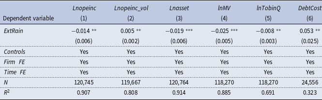
Notes: This table reports the estimates of the effect of rainfall on firm’s balance sheet. The dependent variables are operating income (column (1)), the volatility of operating income (column (2)), fixed assets (column (3)), market values (column (4)), Tobin’s Q (column (5)), and cost of debt (column (6)). The above regressions control for firm-level and province-level control variables, as well as firm and time fixed effects. Cluster-robust standard errors are reported in parentheses clustered at the firm level. See Appendix A.1 for variable definitions. *, **, and *** indicate that the coefficient is significant at the level of 10%, 5%, and 1%.
The unfavorable movement of firm’s balance sheet positions resulting from extreme rainfall would be propagated through the financial market. Specifically, the profit loss and asset impairment would bring about the downward pressure on firm’s stock price. The decline of share price would further depress the asset-liability position, and trigger the “financial accelerator” mechanism, inducing firm cut down its leverage. Building on this insight, we proceed to explore how extreme precipitation affects firm’s performance in the financial market. In column (4) and column (5) in Table 2, we use firm’s market value and Tobin’s Q as the dependent variable, respectively. The negative coefficients on
 $ExtRain$
indicate that firm’s market value (
$ExtRain$
indicate that firm’s market value (
 $lnMV$
) and Tobin’s Q (
$lnMV$
) and Tobin’s Q (
 $lnTobinQ$
) would deteriorate following concentrated rainfall. This implies that severe precipitation events may generate the recession of firm’s balance sheet. Furthermore, we compute firm’s debt financing cost by dividing firm’s interest expenses by its total loans, and regress it on extreme rainfall in column (6). The significantly positive coefficients on
$lnTobinQ$
) would deteriorate following concentrated rainfall. This implies that severe precipitation events may generate the recession of firm’s balance sheet. Furthermore, we compute firm’s debt financing cost by dividing firm’s interest expenses by its total loans, and regress it on extreme rainfall in column (6). The significantly positive coefficients on
 $ExtRain$
indicate that extreme rainfall would push up firm’s funding cost (
$ExtRain$
indicate that extreme rainfall would push up firm’s funding cost (
 $DebtCost$
), and thus induce corporate deleveraging. Overall, the estimation results in Table 2 validate our proposed firm’s balance sheet channel.
$DebtCost$
), and thus induce corporate deleveraging. Overall, the estimation results in Table 2 validate our proposed firm’s balance sheet channel.
Moreover, if the balance sheet channel holds, the negative effect of extreme rainfall on leverage ratio is expected to be stronger for firms that are more financially constrained. We use two measures of financial constraints proposed by Hadlock and Pierce (Reference Hadlock and Pierce2010) and Whited and Wu (Reference Whited and Wu2006), denoted by
 $FC$
Footnote
2
and
$FC$
Footnote
2
and
 $WW$
,Footnote
3
respectively, to study the extent to which financial frictions influence the relationship between severe rainfall and leverage ratio. For both of the above financial constraint measures, a higher value indicates a greater degree of the firm’s financial constraint and higher cost of external finances.
$WW$
,Footnote
3
respectively, to study the extent to which financial frictions influence the relationship between severe rainfall and leverage ratio. For both of the above financial constraint measures, a higher value indicates a greater degree of the firm’s financial constraint and higher cost of external finances.
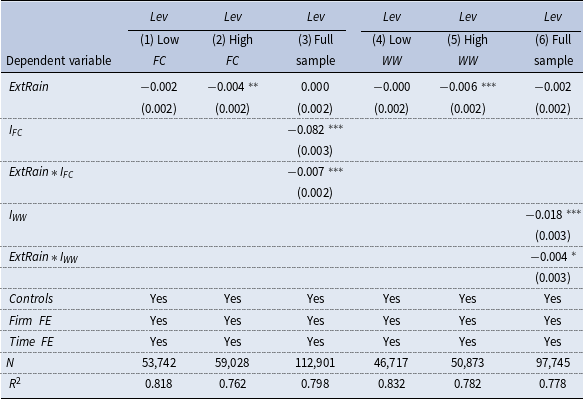
We divided the sample into a high-financing-constraint group and a low-financing-constraint group based on the industry annual mean of
 $FC$
and
$FC$
and
 $WW$
. The results in Table 3 show that the coefficients of
$WW$
. The results in Table 3 show that the coefficients of
 $ExtRain$
in
$ExtRain$
in
 $High\enspace FC$
and
$High\enspace FC$
and
 $High\enspace WW$
groups are statistically significant at 5% and 1% levels, while those in the
$High\enspace WW$
groups are statistically significant at 5% and 1% levels, while those in the
 $Low\enspace FC$
and
$Low\enspace FC$
and
 $Low\enspace WW$
groups are not significant. In columns (3) and (6) in Table 3, we interact
$Low\enspace WW$
groups are not significant. In columns (3) and (6) in Table 3, we interact
 $ExtRain$
with two dummy variables
$ExtRain$
with two dummy variables
 $I_{FC}$
and
$I_{FC}$
and
 $I_{WW}$
, which are defined as whether
$I_{WW}$
, which are defined as whether
 $FC$
and
$FC$
and
 $WW$
are higher than the corresponding median. The significant negative coefficients on the interaction terms indicate that firms with higher levels of financing constraints experienced a greater reduction of leverage after extreme rainfall events.
$WW$
are higher than the corresponding median. The significant negative coefficients on the interaction terms indicate that firms with higher levels of financing constraints experienced a greater reduction of leverage after extreme rainfall events.
2.4.2 Local government crowding-out channel
Another potential explanation for the adverse effects of extreme rainfalls on firm’s leverage is local government’s land financing behaviors in the context of China. Over the past few decades, local governments in China have long used land sale revenues and off-balance sheet borrowing (mainly via local governments financing vehicles, “LGFVs”) to help fund infrastructure projects.Footnote 4 Since land has traditionally been owned by the local governments, LGFVs have also turned to earning revenue by land sales or leases, which can help to repay their creditors. Land can also be used as collateral to secure the bonds. Therefore, a decline in land prices provoked by heavy rainfall would not only trigger the decrease of collateral value but also reduce government revenues and intensify local government’s debt risk, thus forcing banks to tighten lending standards. As LGFVs are implicitly guaranteed by the local government, and banks may choose to cut on funding to private sectors, which will translate into a reduction of corporate leverage.
Table 3. Extreme rainfall, firm’s financing constraints, and leverage

Notes: This table reports the estimates of the firm’s financing constraints heterogeneity in the effect of extreme rainfall on firm’s leverage. According to the industry annual mean of
 $FC$
and
$FC$
and
 $WW$
, we divide the sample into two groups with high and low financing constraints. Grouped regression results are reported in columns (1–2) and column (4–5). Columns (3) and (6) are the estimates of full sample, with additional control for grouping dummy variables and interaction terms. The data are from the CSMAR database. The above regressions control for firm-level and province-level control variables, as well as firm and time fixed effects. Cluster-robust standard errors are reported in parentheses clustered at the firm level. See Appendix A.1 for variable definitions. *, **, and *** indicate that the coefficient is significant at the level of 10%, 5%, and 1%.
$WW$
, we divide the sample into two groups with high and low financing constraints. Grouped regression results are reported in columns (1–2) and column (4–5). Columns (3) and (6) are the estimates of full sample, with additional control for grouping dummy variables and interaction terms. The data are from the CSMAR database. The above regressions control for firm-level and province-level control variables, as well as firm and time fixed effects. Cluster-robust standard errors are reported in parentheses clustered at the firm level. See Appendix A.1 for variable definitions. *, **, and *** indicate that the coefficient is significant at the level of 10%, 5%, and 1%.
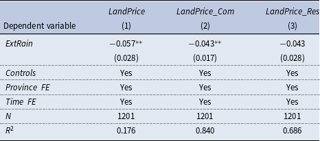
Table 4. Extreme rainfall and land price

Notes: This table reports the estimates of the effect of extreme rainfall on land prices. Data are from the CEIC database. The independent variables are the year-over-year growth rate of total land prices (column (1)), commercial land prices (column (2)), and residential land prices (column (3)). The above regressions control for the
 $GDP$
,
$GDP$
,
 $CPI$
,
$CPI$
,
 $CCPI$
, and
$CCPI$
, and
 $MX$
, with all continuous variables trimmed at 1% on both ends. Province fixed effects and time fixed effects are controlled. Cluster-robust standard errors are reported in parentheses clustered at the province level. See Appendix A.1 for variable definitions. *, **, and *** indicate that the coefficient is significant at the level of 10%, 5%, and 1%.
$MX$
, with all continuous variables trimmed at 1% on both ends. Province fixed effects and time fixed effects are controlled. Cluster-robust standard errors are reported in parentheses clustered at the province level. See Appendix A.1 for variable definitions. *, **, and *** indicate that the coefficient is significant at the level of 10%, 5%, and 1%.
In light of this, we expect that extreme rainfall events would suppress the land price and heighten local government’s debt risk, which would crowd out the funding resources to private firms and exacerbate the deleveraging of firms. To examine the local government crowding-out channel, we first investigate how concentrated rainfall affects the land market. We select land price data from 105 major cities in China and convert it into a provincial quarterly panel. Then we compute the year-over-year growth rate of total land prices, commercial service land prices, and residential land prices, and regress the three on
 $ExtRain$
, respectively. The results are presented in Table 4. As seen from Column (1), the negative relationship between
$ExtRain$
, respectively. The results are presented in Table 4. As seen from Column (1), the negative relationship between
 $ExtRain$
and total land prices (
$ExtRain$
and total land prices (
 $LandPrice$
) is significant, confirming the adverse effects of heavy rainfall on land price. And the drop of total land price mainly comes from the decline of the price of commercial service land (
$LandPrice$
) is significant, confirming the adverse effects of heavy rainfall on land price. And the drop of total land price mainly comes from the decline of the price of commercial service land (
 $LandPrice\_Com$
) instead of the residential land (
$LandPrice\_Com$
) instead of the residential land (
 $LandPrice\_Res$
), as inferred from Column (2) and Column (3). This fact is supported by the findings that extreme weather and climate change, such as floods and hurricanes, result in a notable decline in land values and house prices (Ortega and Taṣpınar, 2005; Hallstrom and Smith, Reference Hallstrom and Smith2005; Zhang et al., Reference Zhang, Deschenes, Meng and Zhang2018).
$LandPrice\_Res$
), as inferred from Column (2) and Column (3). This fact is supported by the findings that extreme weather and climate change, such as floods and hurricanes, result in a notable decline in land values and house prices (Ortega and Taṣpınar, 2005; Hallstrom and Smith, Reference Hallstrom and Smith2005; Zhang et al., Reference Zhang, Deschenes, Meng and Zhang2018).
To shed more light on the local government crowding-out channel, we take the average of issuing yield of municipal bonds in each province to measure the default risk of local government. We then split the sample into high-debt-risk group and low-debt-risk group, based on the cross-sectional median of the province-level municipal bond yield. It is shown that the coefficient on
 $ExtRain$
(−0.005) is statistically significant in high-debt-risk group at the 5% level, which is more than doubled compared with that in low-debt-risk group (−0.002). In column (3), we interact the
$ExtRain$
(−0.005) is statistically significant in high-debt-risk group at the 5% level, which is more than doubled compared with that in low-debt-risk group (−0.002). In column (3), we interact the
 $ExtRain$
with the dummy variable
$ExtRain$
with the dummy variable
 $I_{gov}$
, defined as whether municipal bonds yield is above the median, and the significantly negative coefficient on the interaction term indicates that firms located in provinces with higher debt risk in the government sector would undergo a larger decline of leverage following extreme rainfall events. This confirms the local government crowding-out effects.
$I_{gov}$
, defined as whether municipal bonds yield is above the median, and the significantly negative coefficient on the interaction term indicates that firms located in provinces with higher debt risk in the government sector would undergo a larger decline of leverage following extreme rainfall events. This confirms the local government crowding-out effects.
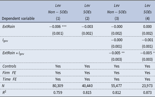
Furthermore, we conjecture that the local government crowding-out effects would be stronger for non-state-owned enterprises (non-SOEs). This is because state-owned enterprises (SOEs), due to their relationship with the government and political connections, have preferential access to bank loans. Consequently, non-SOEs are more likely to adjust their financial leverage when hit by severe rainfall events. Accordingly, we divide the sample into the SOEs group and the non-SOEs group, and add the interaction terms between
 $ExtRain$
and
$ExtRain$
and
 $I_{gov}$
in each sub-sample. As shown in column (1) and column (2), the coefficient on
$I_{gov}$
in each sub-sample. As shown in column (1) and column (2), the coefficient on
 $ExtRain$
remains statistically significant among non-SOEs, while it is insignificant for the SOEs group. And the coefficient on
$ExtRain$
remains statistically significant among non-SOEs, while it is insignificant for the SOEs group. And the coefficient on
 $ExtRain \times I_{gov}$
for non-SOEs is significantly negative at the 5% level, while that in the SOEs group is significant at the 10% level. The different magnitudes of the adverse effects arising from extreme rainfall in SOEs and non-SOEs groups lend further support to the local government crowding-out channel.
$ExtRain \times I_{gov}$
for non-SOEs is significantly negative at the 5% level, while that in the SOEs group is significant at the 10% level. The different magnitudes of the adverse effects arising from extreme rainfall in SOEs and non-SOEs groups lend further support to the local government crowding-out channel.
3. A DSGE model with extreme rainfall shock
We have established the stylized fact that extreme rainfall would lead to a decline of corporate leverage, and have identified firm’s balance sheet channel and local government crowding-out channel. In this section, we interpret our empirical findings through the lens of a structural model with ERS. To be specific, we follow Hashimoto and Sudo (Reference Hashimoto and Sudo2024) and incorporate the ERS that exogenously depresses the levels of capital stock, infrastructure, and TFP at the same time.Footnote 5 Contrary to the earlier standard New Keynesian DSGE models, we introduce China’s land finance system: the interplay among the land market, local government land financing, and infrastructure investments. Such land finance system, deemed to be a key contributor to China’s “economic miracle” over recent decades (Gyourko et al., Reference Gyourko, Shen, Wu and Zhang2022), is an essential element in our model to generate the local government crowding-out effects as documented in Table 5. Moreover, we incorporate the borrowing constraints faced by the private firms following Iacoviello (Reference Iacoviello2015) to account for firm’s balance sheet channel, which is also consistent with the empirical facts about the financing constraints faced by private enterprises in China (Wu, Reference Wu2018).
Table 5. Extreme rainfall, government debt risk, and firm’s leverage
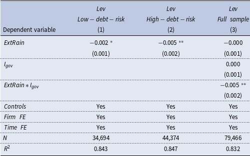
Notes: This table reports the estimates of the government debt risk heterogeneity in the effect of extreme rainfall on firm’s leverage. Data are from the Wind database. Columns (1–2) are the sub-sample regression results of local government bond yield lower/higher than the median. In column (3), the variable of interest is the interaction term,
 $ExtRain*I_{gov}$
, the coefficient of which indicates that the impact of extreme rainfall on firm’s leverage varies with local government debt risk. The above regressions control for firm-level and province-level control variables, as well as firm and time fixed effects. Cluster-robust standard errors are reported in parentheses clustered at the firm level. See Appendix A.1 for variable definitions. *, **, and *** indicate that the coefficient is significant at the level of 10%, 5%, and 1%.
$ExtRain*I_{gov}$
, the coefficient of which indicates that the impact of extreme rainfall on firm’s leverage varies with local government debt risk. The above regressions control for firm-level and province-level control variables, as well as firm and time fixed effects. Cluster-robust standard errors are reported in parentheses clustered at the firm level. See Appendix A.1 for variable definitions. *, **, and *** indicate that the coefficient is significant at the level of 10%, 5%, and 1%.
Specifically, the model consists of the following sectors: a representative household, a continuum of public sector and private sector firms, a continuum of retailers subject to Rotermberg pricing, a representative financial intermediary, local government, and monetary authority. The local government invests in public sector production (e.g., infrastructure investment) and finances government spending through selling land or borrowing from the financial intermediary. Importantly, public sector firms face a working capital constraint, and their infrastructure projects are risky, and thus, they may default on their loans if their idiosyncratic productivity turns out to be lower than the break-even threshold. The private sector firms are subject to borrowing constraints in the sense that the amount of loan is constrained by the market value of their collateral assets. When extreme rainfall event occurs, technology and capital fall immediately, and this will induce the interactions between local government behaviors and private firms’ activities through the land market and financial conditions.
3.1 Model details
3.1.1 Household
The lifetime utility function of the representative household is given by:
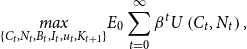 \begin{align} \underset {\left \{ C_{t},N_{t},B_{t},I_{t},u_{t},K_{t+1}\right \} }{max}E_{0}\sum _{t=0}^{\infty }\beta ^{t}U\left (C_{t},N_{t}\right ), \end{align}
where the period utility over consumption
 $C_{t}$
and labor
$C_{t}$
and labor
 $N_{t}$
is given by
$N_{t}$
is given by
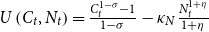 $U\left (C_{t},N_{t}\right )=\frac {C_{t}^{1-\sigma }-1}{1-\sigma }-\kappa _{N}\frac {N_{t}^{1+\eta }}{1+\eta }$
.
$U\left (C_{t},N_{t}\right )=\frac {C_{t}^{1-\sigma }-1}{1-\sigma }-\kappa _{N}\frac {N_{t}^{1+\eta }}{1+\eta }$
.
 $\beta$
is the discounting factor and
$\beta$
is the discounting factor and
 $E_{t}$
is the conditional expectation operator. The parameter
$E_{t}$
is the conditional expectation operator. The parameter
 $\sigma$
controls risk aversion, while the parameter
$\sigma$
controls risk aversion, while the parameter
 $\kappa _{N}$
governs the leisure preference.
$\kappa _{N}$
governs the leisure preference.
 $\eta$
is the inverse Frisch elasticity of labor supply. The household’s budget constraint is given by:
$\eta$
is the inverse Frisch elasticity of labor supply. The household’s budget constraint is given by:
 \begin{align} C_{t}+I_{t}+B_{t}=\frac {W_{t}}{P_{t}}N_{t}+\frac {R_{t-1}B_{t-1}}{\pi _{t}}+r_{t}^{k}u_{t}K_{t}+\varGamma _{t}+T_{t}-uc_{t}K_t, \end{align}
where
 $I_{t}$
denotes investment in capital,
$I_{t}$
denotes investment in capital,
 $w_{t}=\frac {W_{t}}{P_{t}}$
is the real wage,
$w_{t}=\frac {W_{t}}{P_{t}}$
is the real wage,
 $r_{t}^{k}$
is the rental rate on capital
$r_{t}^{k}$
is the rental rate on capital
 $K_{t}$
, and
$K_{t}$
, and
 $u_{t}$
is the capital utilization rate. Financial intermediary pays the risk-free nominal interest rate
$u_{t}$
is the capital utilization rate. Financial intermediary pays the risk-free nominal interest rate
 $R_{t}=1+r_{t}$
on household’s deposits
$R_{t}=1+r_{t}$
on household’s deposits
 $B_{t}$
.
$B_{t}$
.
 $T_{t}$
is the lump-sum transfer from the government, and
$T_{t}$
is the lump-sum transfer from the government, and
 $\varGamma _{t}$
is the profits from the firms in the economy.
$\varGamma _{t}$
is the profits from the firms in the economy.
 $uc_{t}$
is the physical cost of use of capital in resource terms, which is specified as the convex function of capital utilization rate:
$uc_{t}$
is the physical cost of use of capital in resource terms, which is specified as the convex function of capital utilization rate:
 $uc_{t}=\chi _{1}\left (u_{t}-1\right )+\frac {\chi _{2}}{2}\left (u_{t}-1\right )^{2},\chi _{1}\gt 0,\chi _{2}\gt 0$
. We transform the budget constraint into real quantities by dividing by the price of final goods
$uc_{t}=\chi _{1}\left (u_{t}-1\right )+\frac {\chi _{2}}{2}\left (u_{t}-1\right )^{2},\chi _{1}\gt 0,\chi _{2}\gt 0$
. We transform the budget constraint into real quantities by dividing by the price of final goods
 $P_{t}$
.
$P_{t}$
.
Table 6. Extreme rainfall, firm’s ownership, and leverage

Notes: This table reports the estimates of the ownership structure heterogeneity in the effect of extreme rainfall on firm’s leverage. We divide the sample into two groups: non-SOEs and SOEs. Columns (1–2) show inter-group differences in the effect of extreme rainfall on firm’s leverage, while columns (3–4) show inter-group differences in the crowding-out effect of government debt risk. The above regressions control for firm-level and province-level control variables, as well as firm and time fixed effects. Cluster-robust standard errors are reported in parentheses clustered at the firm level. See Appendix A.1 for variable definitions. *, **, and *** indicate that the coefficient is significant at the level of 10%, 5%, and 1%.
Investment
 $I_{t}$
induces the following law of motion for capital:
$I_{t}$
induces the following law of motion for capital:
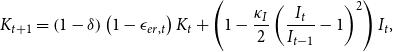 \begin{align} K_{t+1}=\left (1-\delta \right )\left (1-\epsilon _{er,t}\right )K_{t}+\left (1-\frac {\kappa _{I}}{2}\left (\frac {I_{t}}{I_{t-1}}-1\right )^{2}\right )I_{t}, \end{align}
where
 $\delta$
is the capital depreciation rate and
$\delta$
is the capital depreciation rate and
 $\epsilon _{er,t}$
is the ERS. Here, following Hashimoto and Sudo (Reference Hashimoto and Sudo2024), the extreme rainfall
$\epsilon _{er,t}$
is the ERS. Here, following Hashimoto and Sudo (Reference Hashimoto and Sudo2024), the extreme rainfall
 $er_{t}$
is modeled as an AR(1) process:
$er_{t}$
is modeled as an AR(1) process:
 $er_{t}=\rho _{er}er_{t-1}+\sigma _{er}\epsilon _{er,t}$
. The coefficient
$er_{t}=\rho _{er}er_{t-1}+\sigma _{er}\epsilon _{er,t}$
. The coefficient
 $\rho _{er}\in \left (0,1\right )$
is the autoregressive parameter, and
$\rho _{er}\in \left (0,1\right )$
is the autoregressive parameter, and
 $\sigma _{er}$
scales the volatility of ERS. Once this shock occurs, as the direct effect of extreme rainfall events, the capital stock depreciates exogenously by
$\sigma _{er}$
scales the volatility of ERS. Once this shock occurs, as the direct effect of extreme rainfall events, the capital stock depreciates exogenously by
 $\epsilon _{er,t}$
. It’s noteworthy to point out that extreme precipitation and torrential rainfall events have strong seasonal patterns, which usually occur in the summer and last no longer than a few weeks at most. Therefore, extreme rainfall-induced depreciation in capital stock is assumed to occur only within the period (one quarter) in which the ERS
$\epsilon _{er,t}$
. It’s noteworthy to point out that extreme precipitation and torrential rainfall events have strong seasonal patterns, which usually occur in the summer and last no longer than a few weeks at most. Therefore, extreme rainfall-induced depreciation in capital stock is assumed to occur only within the period (one quarter) in which the ERS
 $\epsilon _{er,t}$
occurs.
$\epsilon _{er,t}$
occurs.
The household maximizes its utilities in (2) subjects to the budget constraint in (3) and the law of motion for capital in (4). The optimality conditions for this problem are:
 \begin{equation} 1=\beta E_{t}\left (\frac {C_{t+1}}{C_{t}}\right )^{-\sigma }\frac {R_{t}}{\pi _{t+1}}, \end{equation}
 \begin{equation} uc^{\prime }\left (u_{t}\right )=r_{t}^{k}, \end{equation}
 \begin{equation} \kappa _{N}N_{t}^{\eta }=C_{t}^{-\sigma }w_{t}, \end{equation}
 \begin{equation} q_{t}=E_{t}M_{t+1}\left \{ \left (R_{t+1}^{k}u_{t+1}+q_{t+1}\left (1-\delta \right )\left (1-\epsilon _{er,t+1}\right )\right )\right \} , \end{equation}
 \begin{eqnarray} 1&=&q_{t}\left (1-\frac {\kappa _{I}}{2}\left (\frac {I_{t}}{I_{t-1}}-1\right )^{2}-\kappa _{I}\left (\frac {I_{t}}{I_{t-1}}-1\right )\frac {I_{t}}{I_{t-1}}\right )\nonumber \\[4pt] &&+\beta \kappa _{I}E_{t}\frac {\lambda _{t+1}}{\lambda _{t}}q_{t+1}\left (\frac {I_{t+1}}{I_{t}}-1\right )\left (\frac {I_{t+1}}{I_{t}}\right )^{2}, \end{eqnarray}
where
 $M_{t+1}$
is the stochastic discount factor defined as:
$M_{t+1}$
is the stochastic discount factor defined as:
 $M_{t+1}=\beta E_{t}\frac {\lambda _{t+1}}{\lambda _{t}}=\beta E_{t}\left (\frac {C_{t+1}}{C_{t}}\right )^{-\sigma }$
, and
$M_{t+1}=\beta E_{t}\frac {\lambda _{t+1}}{\lambda _{t}}=\beta E_{t}\left (\frac {C_{t+1}}{C_{t}}\right )^{-\sigma }$
, and
 $\lambda _{t}$
is the Lagrange multiplier associated with the budget constraint.
$\lambda _{t}$
is the Lagrange multiplier associated with the budget constraint.
 $q_{t}$
is the Lagrange multiplier corresponding to the evolution law of capital.
$q_{t}$
is the Lagrange multiplier corresponding to the evolution law of capital.
3.1.2 Production sector
The economy has a continuum of private sector firms, public sector firms, and retailers. Private sector firms are intermediate goods producers, while public sector firms produce the infrastructure goods. Importantly, infrastructure facilities enter the intermediate goods production. Besides the capital and labor input, we assume that both sectors use land as a production factor, and public sector has a larger share of land in production and a lower productivity, while private sector has a smaller share of land in production and a higher productivity. Moreover, private sector firms are credit constrained, and they use land as collateral to finance working capital expenditures.Footnote 6 These features are in line with the stylized facts about Chinese SOE and POE documented in the literature (Wu, Reference Wu2018; Chang et al., Reference Chang, Liu, Spiegel and Zhang2019). Retailers in the model are introduced only to generate nominal price rigidities.
Private sector firm This sector includes a continuum of competitive intermediate goods producers. They use capital, labor, land, and infrastructure goods as input for production and then sell the intermediate goods to retailers at the price of
 $P_{e,t}$
. The representative private sector firm’s production is presented as:
$P_{e,t}$
. The representative private sector firm’s production is presented as:
 \begin{align} Y_{e,t}=\hat {A}_{e,t}\left (L_{e,t}^{\phi _{e}}K_{e,t}^{1-\phi _{e}-\gamma _{e}}M_{g,t}^{\gamma _{e}}\right )^{\alpha }N_{e,t}^{1-\alpha }, \end{align}
where
 $Y_{e,t}$
is the output of the private sector and
$Y_{e,t}$
is the output of the private sector and
 $\hat {A}_{e,t}$
is its TFP.
$\hat {A}_{e,t}$
is its TFP.
 $L_{e,t}$
and
$L_{e,t}$
and
 $K_{e,t}$
denote land and capital inputs, and
$K_{e,t}$
denote land and capital inputs, and
 $M_{g,t}$
is infrastructure stock.
$M_{g,t}$
is infrastructure stock.
 $\phi _{e}$
and
$\phi _{e}$
and
 $\gamma _{e}$
are related to the elasticities of private output with regard to the land and infrastructure stock, respectively.
$\gamma _{e}$
are related to the elasticities of private output with regard to the land and infrastructure stock, respectively.
 $1-\alpha$
is the share of labor input
$1-\alpha$
is the share of labor input
 $N_{e,t}$
in production.
$N_{e,t}$
in production.
We assume that the TFP
 $\hat {A}_{e,t}$
is composed of a permanent component
$\hat {A}_{e,t}$
is composed of a permanent component
 $A_{t}$
and a transitory component
$A_{t}$
and a transitory component
 $A_{e,t}$
, and
$A_{e,t}$
, and
 $\hat {A}_{e,t}$
suffers from the damage from the ERS such that:
$\hat {A}_{e,t}$
suffers from the damage from the ERS such that:
 \begin{equation}\hat {A}_{e,t}=\frac {A_{e,t}A_{t}}{\exp \left ({\theta _{er}er_{t}}\right )}, \end{equation}
 \begin{equation} lnA_{t}=lnA_{t-1}+\sigma _{A}\epsilon _{A,t},\varepsilon _{A,t}\sim N\left (0,1\right ), \end{equation}
 \begin{equation} lnA_{e,t}=\left (1-\rho _{Ae}\right )ln\bar {A}_{e}+\rho _{Ae}lnA_{e,t-1}+\sigma _{Ae}\varepsilon _{Ae,t},\varepsilon _{Ae,t}\sim N\left (0,1\right ), \end{equation}
where the permanent component
 $A_{t}$
follows a random walk process and the transitory component
$A_{t}$
follows a random walk process and the transitory component
 $A_{e,t}$
follows the log AR(1) process, where the parameter
$A_{e,t}$
follows the log AR(1) process, where the parameter
 $\rho _{Ae}$
measures the degrees of persistence and the parameter
$\rho _{Ae}$
measures the degrees of persistence and the parameter
 $\sigma _{Ae}$
measures the standard deviations.
$\sigma _{Ae}$
measures the standard deviations.
 $ln\bar {A}_{e}$
is the steady-state value of
$ln\bar {A}_{e}$
is the steady-state value of
 $lnA_{e,t}$
, and
$lnA_{e,t}$
, and
 $\varepsilon _{Ae,t}$
is i.i.d. standard normal process
$\varepsilon _{Ae,t}$
is i.i.d. standard normal process
 $\varepsilon _{Ae,t}\sim N\left (0,1\right )$
.
$\varepsilon _{Ae,t}\sim N\left (0,1\right )$
.
Note that
 $\theta _{er}\gt 0$
is a parameter that captures the quantitative impacts of extreme rainfall on TFP. Although the damage of extreme rainfall on physical capital is assumed to be transient as in (4), we assume some degree of persistency for the impact of extreme rainfall on TFP. This is in line with the emerging literature documenting that extreme weather and climates disaster have long-lasting adverse effects on productivity through various channels (Bakkensen and Barrage, Reference Bakkensen and Barrage2025; Chen et al., Reference Chen, Lin and Zhu2025).
$\theta _{er}\gt 0$
is a parameter that captures the quantitative impacts of extreme rainfall on TFP. Although the damage of extreme rainfall on physical capital is assumed to be transient as in (4), we assume some degree of persistency for the impact of extreme rainfall on TFP. This is in line with the emerging literature documenting that extreme weather and climates disaster have long-lasting adverse effects on productivity through various channels (Bakkensen and Barrage, Reference Bakkensen and Barrage2025; Chen et al., Reference Chen, Lin and Zhu2025).
We assume that private sector is run by entrepreneurs with the following budget constraint:
 \begin{align} Q_{l,t}\left (L_{e,t+1}-L_{e,t}\right )+w_{t}N_{e,t}+R_{k,t}K_{e,t}+C_{e,t}+\frac {R_{e,t-1}B_{e,t-1}}{\pi _{t}}=\frac {P_{w,t}}{P_{t}}Y_{e,t}+B_{e,t}, \end{align}
where
 $\frac {P_{e,t}}{P_{t}}$
is the relative price of intermediate goods to final goods. Entrepreneurs start the period with intertemporal liabilities
$\frac {P_{e,t}}{P_{t}}$
is the relative price of intermediate goods to final goods. Entrepreneurs start the period with intertemporal liabilities
 $B_{e,t-1}$
with loan rate
$B_{e,t-1}$
with loan rate
 $R_{e,t-1}$
. Before producing, entrepreneurs choose labor
$R_{e,t-1}$
. Before producing, entrepreneurs choose labor
 $N_{e,t}$
, capital inputs
$N_{e,t}$
, capital inputs
 $K_{e,t}$
, incremental land inputs
$K_{e,t}$
, incremental land inputs
 $L_{e,t+1}-L_{e,t}$
, consumption
$L_{e,t+1}-L_{e,t}$
, consumption
 $C_{e,t}$
, and the new intertemporal debt
$C_{e,t}$
, and the new intertemporal debt
 $B_{e,t}$
. As in Kiyotaki and Moore (Reference Kiyotaki and Moore1997) and Iacoviello (Reference Iacoviello2005), the borrowing capacity of the entrepreneurs is constrained by the limited enforceability of debt contracts. The firm is subject to an enforcement constraint:
$B_{e,t}$
. As in Kiyotaki and Moore (Reference Kiyotaki and Moore1997) and Iacoviello (Reference Iacoviello2005), the borrowing capacity of the entrepreneurs is constrained by the limited enforceability of debt contracts. The firm is subject to an enforcement constraint:
 \begin{align} B_{e,t}\leq \theta E_{t}\left (\frac {Q_{l,t+1}L_{e,t+1}\pi _{t+1}}{R_{e,t}}\right )-\zeta \left (w_{t}N_{e,t}+R_{k,t}K_{e,t}\right ). \end{align}
Under this credit constraint, the amount that the private sector firm can borrow is limited by a fraction of the value of the collateral assets—land—nets the operating cost payment, where
 $\zeta \in \left (0,1\right )$
is the fraction of wage bill and capital rent payment in advance. Notice that
$\zeta \in \left (0,1\right )$
is the fraction of wage bill and capital rent payment in advance. Notice that
 $\theta$
could be interpreted as the loan-to-value ratio. The larger
$\theta$
could be interpreted as the loan-to-value ratio. The larger
 $\theta$
, the greater the importance of collateral effects, and the higher the sensitivity of entrepreneurs’ financing conditions to adverse shocks.
$\theta$
, the greater the importance of collateral effects, and the higher the sensitivity of entrepreneurs’ financing conditions to adverse shocks.
Entrepreneurs solve the following maximization problem:
 \begin{align*} \underset {\left \{ C_{e,t},N_{e,t},K_{e,t},B_{e,t},L_{e,t+1}\right \} _{t=0}^{\infty }}{max}E_{0}\sum _{t=0}^{\infty }\beta ^{t}_{e}lnC_{e,t} ,\end{align*}
 \begin{align} s.t \ Q_{l,t}\left (L_{e,t+1}-L_{e,t}\right )+w_{t}N_{e,t}+R_{k,t}K_{e,t}+C_{e,t}+\frac {R_{e,t-1}B_{e,t-1}}{\pi _{t}}=\frac {P_{w,t}}{P_{t}}Y_{e,t}+B_{e,t}, \end{align}
 \begin{align} B_{e,t}\leq \theta E_{t}\left (\frac {Q_{l,t+1}L_{e,t+1}\pi _{t+1}}{R_{e,t}}\right )-\zeta \left (w_{t}N_{e,t}+R_{k,t}K_{e,t}\right ). \end{align}
Here,
 $\beta _{e}\lt \beta$
is the discounting factor of entrepreneurs. We assume that entrepreneurs discount the future more heavily than households to ensure that entrepreneurs will not postpone consumption and quickly accumulate wealth so that they are completely self-financed and the borrowing constraint becomes nonbinding. Entrepreneurs choose
$\beta _{e}\lt \beta$
is the discounting factor of entrepreneurs. We assume that entrepreneurs discount the future more heavily than households to ensure that entrepreneurs will not postpone consumption and quickly accumulate wealth so that they are completely self-financed and the borrowing constraint becomes nonbinding. Entrepreneurs choose
 $C_{e,t},N_{e,t},K_{e,t},B_{e,t},L_{e,t+1}$
to maximize their utility function subjects to the budget constraints and financial constraints outlined above. A detailed characterization of the firm’s optimization problem is outlined in the Supplementary Materials.
$C_{e,t},N_{e,t},K_{e,t},B_{e,t},L_{e,t+1}$
to maximize their utility function subjects to the budget constraints and financial constraints outlined above. A detailed characterization of the firm’s optimization problem is outlined in the Supplementary Materials.
Retailer There is a continuum of retailers indexed by
 $i\in [0,1]$
in the economy. They purchase intermediate goods at the price of
$i\in [0,1]$
in the economy. They purchase intermediate goods at the price of
 $P_{e,t}$
and produce differentiated retail goods
$P_{e,t}$
and produce differentiated retail goods
 $Y_{t}\left (i\right )$
. Retailers simply re-package intermediate output. They take one unit of intermediate output to make a unit of retail output. Final outputs
$Y_{t}\left (i\right )$
. Retailers simply re-package intermediate output. They take one unit of intermediate output to make a unit of retail output. Final outputs
 $Y_{t}$
used for consumption and investment are CES aggregates of retail goods such that:
$Y_{t}$
used for consumption and investment are CES aggregates of retail goods such that:
 \begin{align} Y_{t}=\left (\int _{0}^{1}Y_{t}\left (i\right )^{\frac {\epsilon _{p}-1}{\varepsilon _{p}}}di\right )^{\frac {\varepsilon _{p}}{\varepsilon _{p}-1}}, \end{align}
where
 $\epsilon _{p}$
is the elasticity of substitution among retail goods. From cost minimization by users of final output, we could get the demand curve for each retail good
$\epsilon _{p}$
is the elasticity of substitution among retail goods. From cost minimization by users of final output, we could get the demand curve for each retail good
 $Y_{t}\left (i\right )$
:
$Y_{t}\left (i\right )$
:
 \begin{align} Y_{t}\left (i\right )=\left (\frac {P_{t}\left (i\right )}{P_{t}}\right )^{-\varepsilon _{p}}Y_{t}. \end{align}
In addition, retailers pay quadratic adjustment costs
 $AC_{t}\left (i\right )$
in nominal terms as in Rotemberg (Reference Rotemberg1982),
$AC_{t}\left (i\right )$
in nominal terms as in Rotemberg (Reference Rotemberg1982),
 $AC_{t}\left (i\right )=\frac {\kappa _{P}}{2}\left (\frac {P_{t}\left (i\right )}{P_{t-1}\left (i\right )}-\bar {\pi }\right )^{2}Y_{t}$
, such that price changes deviate from steady-state inflation rate are costly. Subject to the demand function, the retailer
$AC_{t}\left (i\right )=\frac {\kappa _{P}}{2}\left (\frac {P_{t}\left (i\right )}{P_{t-1}\left (i\right )}-\bar {\pi }\right )^{2}Y_{t}$
, such that price changes deviate from steady-state inflation rate are costly. Subject to the demand function, the retailer
 $j$
maximizes its discounted profits flow given by:
$j$
maximizes its discounted profits flow given by:
 \begin{align} \underset {\left \{ P_{t}\left (i\right )\right \} _{t=0}^{\infty }}{max}E_{0}\sum _{t=0}^{\infty }\beta ^{t}\frac {\lambda _{t}}{\lambda _{0}}\left [\frac {P_{t}\left (i\right )-P_{e,t}\left (i\right )}{P_{t}}\left (\frac {P_{t}\left (i\right )}{P_{t}}\right )^{-\varepsilon _{p}}Y_{t}-\frac {\kappa _{P}}{2}\left (\frac {P_{t}\left (i\right )}{P_{t-1}\left (i\right )}-\bar {\pi }\right )^{2}Y_{t}\right ]. \end{align}
In a symmetric equilibrium, all the retailers choose the same price, same inputs, and same output. Define
 $\frac {P_{e,t}}{P_{t}}=mc_{t}$
, we could obtain the following nonlinear Phillips curve:
$\frac {P_{e,t}}{P_{t}}=mc_{t}$
, we could obtain the following nonlinear Phillips curve:
 \begin{align} \frac {\varepsilon _{p}}{\kappa _{P}}\left (mc_{t}-\frac {\varepsilon _{p}-1}{\varepsilon _{p}}\right )+\beta E_{t}\frac {\lambda _{t+1}}{\lambda _{t}}\left (\pi _{t+1}-\bar {\pi }\right )\pi _{t+1}\frac {Y_{t+1}}{Y_{t}}=\left (\pi _{t}-\bar {\pi }\right )\pi _{t}. \end{align}
Public sector firm A continuum of public sector firm indexed by
 $j\in [0,1]$
use land, capital, and labor as input for infrastructure goods production:
$j\in [0,1]$
use land, capital, and labor as input for infrastructure goods production:
 \begin{align} I_{g,t}\left (j\right )=\omega _{t}\left (j\right )\hat {A}_{g,t}\left (L_{g,t}^{\phi _{g}}\left (j\right )K_{g,t}^{1-\phi _{g}}\left (j\right )\right )^{\alpha }N_{g,t}^{1-\alpha }\left (j\right ), \end{align}
where
 $I_{g,t}\left (j\right )$
is the infrastructure output of producer
$I_{g,t}\left (j\right )$
is the infrastructure output of producer
 $j$
. Besides the total productivity of
$j$
. Besides the total productivity of
 $A_{g,t}$
, each producer
$A_{g,t}$
, each producer
 $j$
faces a firm-specific idiosyncratic productivity shock
$j$
faces a firm-specific idiosyncratic productivity shock
 $\omega _{t}\left (j\right )$
that is an i.i.d random variable drawn from a log normal distribution
$\omega _{t}\left (j\right )$
that is an i.i.d random variable drawn from a log normal distribution
 $F(\!\cdot\!)$
with a mean of 1.
$F(\!\cdot\!)$
with a mean of 1.
Similar to private sector firm, we assume that the productivity
 $\hat {A}_{g,t}$
consists of a permanent component
$\hat {A}_{g,t}$
consists of a permanent component
 $A_{t}$
and a transitory component
$A_{t}$
and a transitory component
 $A_{g,t}$
, and
$A_{g,t}$
, and
 $\hat {A}_{g,t}$
is also adversely affected by the extreme weather shock such that
$\hat {A}_{g,t}$
is also adversely affected by the extreme weather shock such that
 \begin{equation}\hat {A}_{g,t}=\frac {A_{g,t}A_{t}} {\exp \left ({\theta _{er}er_{t}}\right )}, \end{equation}
 \begin{equation} ln A_{t}=lnA_{t-1}+\sigma _{A}\epsilon _{A,t},\varepsilon _{A,t}\sim i.i.d\ N\left (0,1\right ), \end{equation}
 \begin{equation} ln A_{g,t}=\left (1-\rho _{Ag}\right )ln\bar {A_{g}}+\rho lnA_{g,t-1}+\sigma _{Ag}\varepsilon _{Ag,t},\varepsilon _{Ag,t}\sim i.i.d\ N\left (0,1\right ), \end{equation}
where the permanent component
 $A_{t}$
is imposed to be the same as that of private sector firm, to ensure the common trend growth rate along the balanced growth path. The transitory component
$A_{t}$
is imposed to be the same as that of private sector firm, to ensure the common trend growth rate along the balanced growth path. The transitory component
 $A_{g,t}$
follows a log AR(1) process with persistence
$A_{g,t}$
follows a log AR(1) process with persistence
 $\rho _{Ag}$
, standard deviation
$\rho _{Ag}$
, standard deviation
 $\sigma _{Ag}$
, and
$\sigma _{Ag}$
, and
 $\varepsilon _{Ag,t}\sim i.i.d\ N\left (0,1\right )$
.
$\varepsilon _{Ag,t}\sim i.i.d\ N\left (0,1\right )$
.
Importantly, public sector firms face working capital constraints, as all the payments are made before the production takes place. Since idiosyncratic shocks are i.i.d, all public infrastructure producers face the same ex ante cost minimization problem as such:
 \begin{align*} \underset {K_{g,t},L_{g,t},N_{g,t}}{min}R_{k,t}K_{g,t}+R_{l,t}L_{g,t}+w_{t}N_{g,t} ,\end{align*}
 \begin{align} s.t. \ I_{g,t}=E\left (\omega _{t}\left (j\right )\right )A_{g,t}\left (L_{g,t}^{\phi }K_{g,t}^{1-\phi }\right )^{\alpha }N_{g,t}^{1-\alpha }, \end{align}
where the rental price for capital and land
 $R_{k,t}$
and
$R_{k,t}$
and
 $R_{l,t}$
, and the wage
$R_{l,t}$
, and the wage
 $w_{t}$
are given. Let
$w_{t}$
are given. Let
 $\lambda _{g,t}$
be the Lagrangian multiplier associated with the production function, the optimality conditions are:
$\lambda _{g,t}$
be the Lagrangian multiplier associated with the production function, the optimality conditions are:
 \begin{equation} R_{k,t}=\lambda _{g,t}\alpha \left (1-\phi \right )\frac {I_{g,t}}{K_{g,t}}, \end{equation}
 \begin{equation} R_{l,t}=\lambda _{g,t}\alpha \phi \frac {I_{g,t}}{L_{g,t}}, \end{equation}
 \begin{equation} w_{t}=\lambda _{g,t}\left (1-\alpha \right )\frac {I_{g,t}}{N_{g,t}}. \end{equation}
The law of motion for infrastructure stock follows:
 \begin{align} M_{g,t}=\left (1-\delta _{g}\right )(1-\epsilon _{er,t})M_{g,t-1}+I_{g,t}, \end{align}
where
 $\delta _{g}$
is the depreciation rate of infrastructure stock. Note that extreme weather shock
$\delta _{g}$
is the depreciation rate of infrastructure stock. Note that extreme weather shock
 $\epsilon _{er,t}$
could lead to the damage of public infrastructure. For example, heavy rainfall may trigger widespread flooding and disrupt the transit options and cause damage to roads and streetlights.Footnote
7
To finance the working capital, public sector firm resorts to its own beginning-of-period net worth
$\epsilon _{er,t}$
could lead to the damage of public infrastructure. For example, heavy rainfall may trigger widespread flooding and disrupt the transit options and cause damage to roads and streetlights.Footnote
7
To finance the working capital, public sector firm resorts to its own beginning-of-period net worth
 $V_{g,t}$
and borrows from financial intermediaries
$V_{g,t}$
and borrows from financial intermediaries
 $B_{g,t}$
. As the idiosyncratic productivity shock is i.i.d., all firms would borrow the same amount of debt
$B_{g,t}$
. As the idiosyncratic productivity shock is i.i.d., all firms would borrow the same amount of debt
 $B_{g,t}$
:
$B_{g,t}$
:
 \begin{align} \frac {V_{g,t}+B_{g,t}}{P_{t}}=R_{k,t}K_{g,t}+R_{l,t}L_{g,t}+w_{t}N_{g,t}. \end{align}
Define the relative price between infrastructure goods and final goods
 $p_{t}^{g}=\frac {P_{g,t}}{P_{t}}$
, and let
$p_{t}^{g}=\frac {P_{g,t}}{P_{t}}$
, and let
 $R_{z,t}=\frac {p_{t}^{g}}{\lambda _{g,t}}$
, then public sector firm’s balance sheet can be re-written as:
$R_{z,t}=\frac {p_{t}^{g}}{\lambda _{g,t}}$
, then public sector firm’s balance sheet can be re-written as:
 \begin{align} P_{g,t}I_{g,t}=R_{z,t}\left (V_{g,t}+B_{g,t}\right ). \end{align}
Now we characterize the debt contract between financial intermediary and public sector. At the beginning of each period, the financial intermediary lends to public sector firms at the interest rate of
 $Z_{t}$
, which choose the level of debt
$Z_{t}$
, which choose the level of debt
 $B_{g,t}$
prior to the realization of idiosyncratic firm-specific productivity shocks. The optimal contract between the bank and public sector firm is then characterized by a threshold on idiosyncratic productivity
$B_{g,t}$
prior to the realization of idiosyncratic firm-specific productivity shocks. The optimal contract between the bank and public sector firm is then characterized by a threshold on idiosyncratic productivity
 $\varpi _{t}$
, such that the firm with the cutoff productivity is just able to repay the external debt
$\varpi _{t}$
, such that the firm with the cutoff productivity is just able to repay the external debt
 $B_{g,t}$
:
$B_{g,t}$
:
 \begin{align} \varpi _{t}P_{g,t}I_{g,t}=Z_{t}B_{g,t}. \end{align}
The threshold productivity level is given by:
 \begin{align} \varpi _{t}=\frac {Z_{t}B_{g,t}}{R_{z,t}\left (V_{g,t}+B_{g,t}\right )}. \end{align}
When
 $\omega _{t}\geq \varpi _{t}$
, the firm repays the loan, and the bank receives the payoff of
$\omega _{t}\geq \varpi _{t}$
, the firm repays the loan, and the bank receives the payoff of
 $Z_{t}B_{g,t}$
. When
$Z_{t}B_{g,t}$
. When
 $\omega _{t}\lt \varpi _{t}$
, the firm cannot pay the contractual return and has to default. In this case, the bank pays a monitoring cost, defined as a fraction
$\omega _{t}\lt \varpi _{t}$
, the firm cannot pay the contractual return and has to default. In this case, the bank pays a monitoring cost, defined as a fraction
 $\mu$
of the firm’s total revenue, to observe the realized idiosyncratic productivity shock and collect the firm’s revenue. Overall, the expected nominal income for the bank is given by:
$\mu$
of the firm’s total revenue, to observe the realized idiosyncratic productivity shock and collect the firm’s revenue. Overall, the expected nominal income for the bank is given by:
 \begin{eqnarray} &&\kern-24pt \left (1-F\left (\varpi _{t}\right )\right )Z_{t}B_{g,t}+\int _{0}^{\varpi _{t}}\left (1-\mu \right )\omega _{t}P_{g,t}I_{g,t}dF\left (\omega _{t}\right ) \nonumber \\[5pt] &&= R_{z,t}\left (V_{g,t}+B_{g,t}\right )\underset {g\left (\varpi _{t}\right )}{\underbrace {\left (\left (1-F\left (\varpi _{t}\right )\right )\varpi _{t}+\int _{0}^{\varpi _{t}}\left (1-\mu \right )\omega _{t}dF\left (\omega _{t}\right )\right )}}. \end{eqnarray}
As a result, the bank would lend to firms if the expected income per unit of fund can at least cover the required rate of return
 $R_{g,t}$
which is endogenous determined by the financial intermediary:
$R_{g,t}$
which is endogenous determined by the financial intermediary:
 \begin{align} R_{z,t}\left (V_{g,t}+B_{g,t+1}\right )g\left (\varpi _{t}\right )\geq R_{g,t}B_{g,t}. \end{align}
The optimal contract is a pair
 $\left (\varpi _{t},B_{g,t}\right )$
chosen at the beginning of period
$\left (\varpi _{t},B_{g,t}\right )$
chosen at the beginning of period
 $t$
to maximize the firm’s expected income subjects to the lender’s participation constraint. In particular, the optimal contract solves the problem:
$t$
to maximize the firm’s expected income subjects to the lender’s participation constraint. In particular, the optimal contract solves the problem:
 \begin{align*} \underset {\varpi _{t},B_{g,t}}{max} R_{z,t}\left (V_{g,t}+B_{g,t}\right )\underset {f\left (\varpi _{t}\right )}{\underbrace {\left (\int _{\varpi _{t}}^{\infty }\omega _{t}dF\left (\omega _{t}\right )-\left (1-F\left (\varpi _{t}\right )\right )\varpi _{t}\right )}} ,\end{align*}
 \begin{align} s.t \ R_{z,t}\left (V_{g,t}+B_{g,t}\right )g\left (\varpi _{t}\right )\geq R_{g,t}B_{g,t}. \end{align}
In the expression above,
 $f\left (\varpi _{t}\right )$
and
$f\left (\varpi _{t}\right )$
and
 $g\left (\varpi _{t}\right )$
can be viewed as the income share that goes to the firm and bank, respectively. The following first-order condition characterizes the optimal contract:
$g\left (\varpi _{t}\right )$
can be viewed as the income share that goes to the firm and bank, respectively. The following first-order condition characterizes the optimal contract:
 \begin{align} \frac {g^{\prime }\left (\varpi _{t}\right )f\left (\varpi _{t}\right )}{f^{\prime }\left (\varpi _{t}\right )}\frac {R_{z,t}}{R_{g,t}}=-\frac {V_{g,t}}{B_{g,t}+V_{g,t}}, \end{align}
which illustrates firm’s demand for external debt. We assume that only a share
 $\chi _g$
of public sector firms survive at each period. The end-of-period aggregate net worth of public sector firms depends on profits earned by surviving firms plus managerial income. Thus, the net worth evolves according to the law of motion as follows:
$\chi _g$
of public sector firms survive at each period. The end-of-period aggregate net worth of public sector firms depends on profits earned by surviving firms plus managerial income. Thus, the net worth evolves according to the law of motion as follows:
 \begin{align} V_{g,t+1}=\chi _g R_{z,t}\left (V_{g,t}+B_{g,t}\right )f\left (\varpi _{t}\right ). \end{align}
In addition, we define the default rate of public sector firms as
 $Bankrupt_{t}=F\left (\varpi _{t}\right )$
, which is the probability of the event
$Bankrupt_{t}=F\left (\varpi _{t}\right )$
, which is the probability of the event
 $\omega _{t}\lt \varpi _{t}$
.
$\omega _{t}\lt \varpi _{t}$
.
3.1.3 Financial intermediary
We model financial intermediaries in a similar way as Gertler and Karadi (Reference Gertler and Karadi2011). Financial intermediation takes place through a continuum of competitive representative commercial banks. Each period, a fraction of financial intermediaries stochastically exit and are replaced by the same number of new intermediaries with startup funds from households. Financial intermediaries accumulate net worth until they exit, whereby they return their net worth to household owners. The intermediary
 $j\in [0,1]$
lends to the private sector and public sector,
$j\in [0,1]$
lends to the private sector and public sector,
 $B^{j}_{e,t}$
and
$B^{j}_{e,t}$
and
 $B^{j}_{g,t}$
as well as local government sector
$B^{j}_{g,t}$
as well as local government sector
 $B^{j}_{G,t}$
, which are financed by the deposits from households
$B^{j}_{G,t}$
, which are financed by the deposits from households
 $B^{j}_{t}$
and intermediary
$B^{j}_{t}$
and intermediary
 $j$
’s net worth
$j$
’s net worth
 $V^{j}_{t}$
. The balance sheet condition of intermediary
$V^{j}_{t}$
. The balance sheet condition of intermediary
 $j$
is given by:
$j$
is given by:
 \begin{align} B^{j}_{g,t}+B^{j}_{e,t}+B^{j}_{G,t}=V^{j}_{t}+B^{j}_{t}. \end{align}
If intermediary
 $j$
survives, then its net worth evolves as,
$j$
survives, then its net worth evolves as,
 \begin{align} V^{j}_{t+1}=\left (R_{g,t}-R_{t-1}\right )B^{j}_{g,t}+\left (R_{e,t}-R_{t-1}\right )B^{j}_{e,t}+\left (R_{G,t}-R_{t-1}\right )B^{j}_{G,t}+R_{t-1}V^{j}_{t}, \end{align}
where
 $R_{e,t},R_{g,t}$
, and
$R_{e,t},R_{g,t}$
, and
 $R_{G,t}$
are the lending rate to the private sector, public sector, and local government, respectively. Each period, a fraction
$R_{G,t}$
are the lending rate to the private sector, public sector, and local government, respectively. Each period, a fraction
 $1-\chi _f$
of financial intermediaries exit and return their net worth to domestic household owners. The objective of the intermediary
$1-\chi _f$
of financial intermediaries exit and return their net worth to domestic household owners. The objective of the intermediary
 $j$
is to maximize its expected terminal net worth discounted by the stochastic discount factor of the household:
$j$
is to maximize its expected terminal net worth discounted by the stochastic discount factor of the household:
 \begin{eqnarray}&&\kern-24pt \ell ^{j}_{t}\left (V^{j}_{t},B^{j}_{g,t},B^{j}_{e,t},B^{j}_{G,t}\right ) =E_{t}M_{t,t+1}\bigg \{\left (1-\chi _f\right )V^{j}_{t+1} \nonumber \\ && + \chi _f\underset {\left \{ B^{j}_{g,t+1},B^{j}_{e,t+1},B^{j}_{G,t+1}\right \}}{max}\ell ^{j}_{t+1}\bigg (V^{j}_{t+1},B^{j}_{g,t+1},B^{j}_{e,t+1},B^{j}_{G,t+1}\bigg )\bigg \}, \end{eqnarray}
where
 $\ell ^{j}_{t}\left (\cdot \right )$
is the value function of intermediary
$\ell ^{j}_{t}\left (\cdot \right )$
is the value function of intermediary
 $j$
. As in Gertler and Karadi (Reference Gertler and Karadi2011), we assume that an intermediary can divert a fraction
$j$
. As in Gertler and Karadi (Reference Gertler and Karadi2011), we assume that an intermediary can divert a fraction
 $\theta _{f}$
of its assets and transfer them to household owners, in which case depositors can recover the remaining assets and force the intermediary into bankruptcy. Thus, an incentive constraint must be satisfied for depositors to be willing to lend in the first place:
$\theta _{f}$
of its assets and transfer them to household owners, in which case depositors can recover the remaining assets and force the intermediary into bankruptcy. Thus, an incentive constraint must be satisfied for depositors to be willing to lend in the first place:
 \begin{align} \ell ^{j}_{f,t}\geq \theta _{f}\left (\Delta _{g}B^{j}_{g,t}+\Delta _{e}B^{j}_{e,t}+B^{j}_{G,t}\right ). \end{align}
We assume that it is easier for the intermediary to divert loan Assets to the private and public sector than government bonds, thus
 $\Delta _{g}\gt 0$
and
$\Delta _{g}\gt 0$
and
 $\Delta _{e}\gt 0$
. The parameter
$\Delta _{e}\gt 0$
. The parameter
 $\theta _{f}$
captures the tightness of the credit market: when
$\theta _{f}$
captures the tightness of the credit market: when
 $\theta _{f}$
increases, depositors can recover a smaller fraction of an intermediary’s assets in the event of bankruptcy, which in turn makes them less willing to lend funds. All financial intermediaries will behave in the same way with identical optimality conditions. These are
$\theta _{f}$
increases, depositors can recover a smaller fraction of an intermediary’s assets in the event of bankruptcy, which in turn makes them less willing to lend funds. All financial intermediaries will behave in the same way with identical optimality conditions. These are
 \begin{equation} \left (1+\omega _{f,t}\right )E_{t}M_{t,t+1}\left (1-\chi _{f}+\chi _{f}\phi _{f,t+1}\right )\left (R_{g,t}-R_{t-1}\right )=\omega _{f,t}\theta _{f}\Delta _{g}, \end{equation}
 \begin{equation} \left (1+\omega _{f,t}\right )E_{t}M_{t,t+1}\left (1-\chi _{f}+\chi _{f}\phi _{f,t+1}\right )\left (R_{e,t}-R_{t-1}\right )=\omega _{f,t}\theta _{f}\Delta _{e}, \end{equation}
 \begin{equation} \left (1+\omega _{f,t}\right )E_{t}M_{t,t+1}\left (1-\chi _{f}+\chi _{f}\phi _{f,t+1}\right )\left (R_{G,t}-R_{t-1}\right )=\omega _{f,t}\theta _{f}, \end{equation}
 \begin{equation} \phi _{f,t}=\left (1+\omega _{f,t}\right )E_{t}M_{t,t+1}\left (1-\chi _{f}+\chi _{f}\phi _{f,t+1}\right )R_{t-1}, \end{equation}
where
 $\omega _{f,t}$
is the Lagrange multiplier associated with the incentive constraint. The derivation of these conditions is presented in detail in the Supplementary Materials. Finally, we assume that newly entering intermediaries receive start-up funds from households, which is assumed to be a fraction
$\omega _{f,t}$
is the Lagrange multiplier associated with the incentive constraint. The derivation of these conditions is presented in detail in the Supplementary Materials. Finally, we assume that newly entering intermediaries receive start-up funds from households, which is assumed to be a fraction
 $\varsigma$
of their net worth. The aggregate net worth in the financial sector evolves as,
$\varsigma$
of their net worth. The aggregate net worth in the financial sector evolves as,
 \begin{align} V_{f,t+1} & =\chi _{f}\left (\left (R_{g,t}-R_{t-1}\right )B_{g,t}+\left (R_{e,t}-R_{t-1}\right )B_{e,t}+\left (R_{G,t}-R_{t-1}\right )B_{G,t}+R_{t-1}V_{f,t}\right )+\varsigma V_{f,t}. \end{align}
3.1.4 Local government
Land is initially developed by the local government. The local government sells part of the developed land to raise revenue. The government spends on the consumption of infrastructure goods and finances this spending through land sale revenue, personal taxes, and borrowing from the bank. The government budget constraint is:
 \begin{align} Q_{l,t}\left (L_{e,t}-L_{e,t-1}\right )+T_{t}+R_{l,t}L_{g,t}+B_{G,t}=G_{t}+p_{t}^{g}I_{g,t}+R_{G,t-1}B_{G,t-1}, \end{align}
where
 $G_{t}$
and
$G_{t}$
and
 $p_{t}^{g}I_{g,t}$
denote government consumption of final goods and infrastructure goods, respectively.
$p_{t}^{g}I_{g,t}$
denote government consumption of final goods and infrastructure goods, respectively.
 $R_{G,t}$
is the return of one-period government bond which is assumed to be a log-AR(1) process:
$R_{G,t}$
is the return of one-period government bond which is assumed to be a log-AR(1) process:
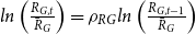 $ln\left (\frac {R_{G,t}}{\bar {R}_{G}}\right )=\rho _{RG}ln\left (\frac {R_{G,t-1}}{\bar {R}_{G}}\right )$
, with persistence parameter
$ln\left (\frac {R_{G,t}}{\bar {R}_{G}}\right )=\rho _{RG}ln\left (\frac {R_{G,t-1}}{\bar {R}_{G}}\right )$
, with persistence parameter
 $\rho _{RG}$
. Assume that the government consumption to output ratio follows AR(1) processes and the fiscal policy shock
$\rho _{RG}$
. Assume that the government consumption to output ratio follows AR(1) processes and the fiscal policy shock
 $\varepsilon _{g,t}$
is i.i.d. with a zero mean and a normal process of standard deviation:
$\varepsilon _{g,t}$
is i.i.d. with a zero mean and a normal process of standard deviation:
 \begin{equation} G_{t}=g_{t}Y_{t}, \end{equation}
 \begin{equation} ln\left (\frac {g_{t}}{\bar {g}}\right )=\rho _{g}ln\left (\frac {g_{t-1}}{\bar {g}}\right )+\varepsilon _{g,t},\varepsilon _{g,t}\sim N\left (0,\sigma _{g}^{2}\right ). \end{equation}
The tax-output ratio follows a fiscal rule to keep the government debt from continuously growing:
 \begin{equation} T_{t}=\tau _{t}Y_{t}, \end{equation}
 \begin{equation} ln\left (\frac {\tau _{t}}{\bar {\tau }}\right )=\rho _{\tau }ln\left (\frac {\tau _{t-1}}{\bar {\tau }}\right )+\rho _{\tau b}\left (ln\left (\frac {B_{G,t}}{Y_{t}}\right )-ln\left (\frac {\bar {B}_{G}}{\bar {Y}}\right )\right )+\varepsilon _{\tau,t},\varepsilon _{\tau,t}\sim N\left (0,\sigma _{\tau}^{2}\right ). \end{equation}
The shock to the tax-output ratio
 $\varepsilon _{\tau ,t}$
is i.i.d. with a zero mean and a normal process of standard deviation.
$\varepsilon _{\tau ,t}$
is i.i.d. with a zero mean and a normal process of standard deviation.
3.1.5 Monetary authority
The central bank conducts monetary policy following a standard Taylor rule:
 \begin{align} ln\left (\frac {R_{t}}{\bar {R}}\right )=\rho _{m}ln\left (\frac {R_{t-1}}{\bar {R}}\right )+\left (1-\rho _{m}\right )\left (\varphi _{\pi }ln\left (\frac {\pi _{t}}{\bar {\pi }}\right )+\varphi _{y}ln\left (\frac {Y_{t}}{\bar {Y}}\right )\right )+\varepsilon _{m,t},\varepsilon _{m,t}\sim N\left (0,\sigma _{m}^{2}\right ), \end{align}
where
 $\varphi _{\pi }$
and
$\varphi _{\pi }$
and
 $\varphi _{y}$
are responsive coefficients of central bankers to inflation gap and output gap, respectively, and
$\varphi _{y}$
are responsive coefficients of central bankers to inflation gap and output gap, respectively, and
 $\rho _{m}$
measures the degree of interest rate inertia.
$\rho _{m}$
measures the degree of interest rate inertia.
3.1.6 Market clearing
The capital market clearing condition is:
 \begin{align} K_{e,t}+K_{g,t}=u_{t}K_{t-1}. \end{align}
The labor market clearing condition is:
 \begin{align} N_{e,t}+N_{g,t}=N_{t}. \end{align}
The land market clearing condition is:
 \begin{align} L_{e,t}+L_{g,t}=L. \end{align}
The land supply is fixed at
 $L.$
The aggregate resource constraint clears the goods market:
$L.$
The aggregate resource constraint clears the goods market:
 \begin{align} Y_{t}=C_{t}+I_{t}+p_{t}^{g}I_{g,t}+G_{t}+\frac {\kappa _{P}}{2}\left (\pi _{t}-\bar {\pi }\right )^{2}Y_{t}. \end{align}
Before computing the model, we normalize all relevant variables to obtain stationarity following the normalization scheme in (Fernández-Villaverde and Rubio-Ramírez, Reference Fernández-Villaverde and Rubio-Ramírez2006). The full equilibrium conditions and the detrended system are listed in the Supplementary Materials.
3.2 Parameter calibration and estimation
The model is calibrated at a quarterly frequency. The steady state of inflation rate
 $\bar{\pi}$
is normalized to 1. The discount factor of household
$\bar{\pi}$
is normalized to 1. The discount factor of household
 $\beta$
is 0.9961, implying a risk-free rate of 1.6% annually. Following Iacoviello (Reference Iacoviello2015). We set the discount factor of entrepreneur
$\beta$
is 0.9961, implying a risk-free rate of 1.6% annually. Following Iacoviello (Reference Iacoviello2015). We set the discount factor of entrepreneur
 $\beta _e$
to 0.94. We set
$\beta _e$
to 0.94. We set
 $\eta$
to 2, implying a Frisch elasticity of labor supply of 0.5, consistent with microeconomic evidence (Pencavel, Reference Pencavel1986). The elasticity of substitution among intermediate goods
$\eta$
to 2, implying a Frisch elasticity of labor supply of 0.5, consistent with microeconomic evidence (Pencavel, Reference Pencavel1986). The elasticity of substitution among intermediate goods
 $\epsilon _{p}$
is 11, yielding an average markup of 10%, which is consistent with the estimate reported by Basu and Fernald (Reference Basu and Fernald1997). The relative risk aversion parameter
$\epsilon _{p}$
is 11, yielding an average markup of 10%, which is consistent with the estimate reported by Basu and Fernald (Reference Basu and Fernald1997). The relative risk aversion parameter
 $\sigma$
is set to 2, which is standard in the literature. The depreciation rate for private and public capital is set to 0.05 and 0.025, respectively, given that public capital depreciates relatively slowly. Labor share
$\sigma$
is set to 2, which is standard in the literature. The depreciation rate for private and public capital is set to 0.05 and 0.025, respectively, given that public capital depreciates relatively slowly. Labor share
 $1-\alpha$
is calibrated to 0.5, consistent with empirical evidences in Chinese data (Zhu, Reference Zhu2012).
$1-\alpha$
is calibrated to 0.5, consistent with empirical evidences in Chinese data (Zhu, Reference Zhu2012).
 $\phi _{e}$
and
$\phi _{e}$
and
 $\phi _{g}$
, share of land input in the production of private and public sectors, are calibrated to 0.5 and 0.35, respectively, to match the ratio of the value of commercial real estate to output in POE and SOE. These data are taken from the National Bureau of Statistics of China for the period 2000–2023.
$\phi _{g}$
, share of land input in the production of private and public sectors, are calibrated to 0.5 and 0.35, respectively, to match the ratio of the value of commercial real estate to output in POE and SOE. These data are taken from the National Bureau of Statistics of China for the period 2000–2023.
 $\gamma _{e}$
is set to 0.20, such that the output elasticity of infrastructure is 0.1, as reported by Calderón et al. (Reference Calderón, Moral-Benito and Servén2015) for a set of emerging market economies including China. Following Iacoviello (Reference Iacoviello2015), labor wage and capital rent must be fully paid in advance, so that
$\gamma _{e}$
is set to 0.20, such that the output elasticity of infrastructure is 0.1, as reported by Calderón et al. (Reference Calderón, Moral-Benito and Servén2015) for a set of emerging market economies including China. Following Iacoviello (Reference Iacoviello2015), labor wage and capital rent must be fully paid in advance, so that
 $\zeta =1$
. As the minimum down-payment ratio of housing mortgage is about 20%–30% in China, we set the loan-to-value ratio
$\zeta =1$
. As the minimum down-payment ratio of housing mortgage is about 20%–30% in China, we set the loan-to-value ratio
 $\theta$
to 0.75 or so. Fraction of capital that can be diverted is set to 0.38, which is borrowed from Gertler and Karadi (Reference Gertler and Karadi2011). As in Bernanke et al. (Reference Bernanke, Gertler and Gilchrist1999), we set the monitoring cost parameter
$\theta$
to 0.75 or so. Fraction of capital that can be diverted is set to 0.38, which is borrowed from Gertler and Karadi (Reference Gertler and Karadi2011). As in Bernanke et al. (Reference Bernanke, Gertler and Gilchrist1999), we set the monitoring cost parameter
 $\mu _{g}$
to 0.21 or so. We normalize
$\mu _{g}$
to 0.21 or so. We normalize
 $\bar {A}_{g}$
to one and set
$\bar {A}_{g}$
to one and set
 $\bar {A}_{e}$
to 1.2 such that the steady-state hours in the private and public sectors equal to
$\bar {A}_{e}$
to 1.2 such that the steady-state hours in the private and public sectors equal to
 $\frac {1}{3}$
. The price adjustment cost parameter
$\frac {1}{3}$
. The price adjustment cost parameter
 $\kappa _{P}$
is set to 50, and the investment adjustment cost parameter
$\kappa _{P}$
is set to 50, and the investment adjustment cost parameter
 $\kappa _{I}$
is set to 2.5. The utilization adjustment cost
$\kappa _{I}$
is set to 2.5. The utilization adjustment cost
 $\chi _{1}$
is endogenously pinned down by the steady-state capital rental rate, while the squared term in the utilization adjustment cost function is set to
$\chi _{1}$
is endogenously pinned down by the steady-state capital rental rate, while the squared term in the utilization adjustment cost function is set to
 $\chi _{2}=0.01$
, as in Sims and Wu (Reference Sims and Wu2021). We calibrate the bank survival rate
$\chi _{2}=0.01$
, as in Sims and Wu (Reference Sims and Wu2021). We calibrate the bank survival rate
 $\chi _f$
and public sector firm survival rate
$\chi _f$
and public sector firm survival rate
 $\chi _g$
to 0.85 and 0.96, respectively, to match the annualized default rate about 2%, which is in agreement with the historical averages nonperforming loans ratio in Chinese data.
$\chi _g$
to 0.85 and 0.96, respectively, to match the annualized default rate about 2%, which is in agreement with the historical averages nonperforming loans ratio in Chinese data.
We calibrate the steady state of bank loan rate
 $R_e$
to 1.011, steady state of treasury bond rate
$R_e$
to 1.011, steady state of treasury bond rate
 $R_g$
to 1.006, and steady state of public sector financing cost
$R_g$
to 1.006, and steady state of public sector financing cost
 $R_G$
to 1.018, to match the following three targets in China from 2015 to 2024: (1) the quarterly average of one-year bank lending-rate about 4.4%; (2) the quarterly average of one-year government bond yield close to 2.35%; (3) the quarterly average of one-year municipal investment bond yield about 7.5%. We fit an AR(1) process of one-year government bond yield to calibrate the persistence parameter
$R_G$
to 1.018, to match the following three targets in China from 2015 to 2024: (1) the quarterly average of one-year bank lending-rate about 4.4%; (2) the quarterly average of one-year government bond yield close to 2.35%; (3) the quarterly average of one-year municipal investment bond yield about 7.5%. We fit an AR(1) process of one-year government bond yield to calibrate the persistence parameter
 $\rho _{BG}$
to 0.92. We use the quarterly time series of tax revenues-output ratio, government debt-output ratio, and government spending-output ratio in China from 2001 to 2023, to estimate the parameters in the fiscal policy rules. We rely on the following three series: (1) 7-day interbank interest rate, (2) GDP, and (3) CPI inflation rate, spanning the sample 2001Q1–2023Q4, to estimate the parameters in the Taylor rule. These data series are from China macroeconomic time series database constructed by Chang et al. (Reference Chang, Chen, Waggoner and Zha2016).Footnote
8
Calibrated parameter values are listed in Table 7.
$\rho _{BG}$
to 0.92. We use the quarterly time series of tax revenues-output ratio, government debt-output ratio, and government spending-output ratio in China from 2001 to 2023, to estimate the parameters in the fiscal policy rules. We rely on the following three series: (1) 7-day interbank interest rate, (2) GDP, and (3) CPI inflation rate, spanning the sample 2001Q1–2023Q4, to estimate the parameters in the Taylor rule. These data series are from China macroeconomic time series database constructed by Chang et al. (Reference Chang, Chen, Waggoner and Zha2016).Footnote
8
Calibrated parameter values are listed in Table 7.
We pin down the extreme rainfall-related parameters
 $\rho _{er}$
,
$\rho _{er}$
,
 $\theta _{er}$
and
$\theta _{er}$
and
 $\sigma _{er}$
, and the parameters in the TFP process
$\sigma _{er}$
, and the parameters in the TFP process
 $\left \{ \rho _{Ae},\rho _{Ag},\sigma _{Ae},\sigma _{Ag}\right \}$
by the Simulated Method of Moments approach as proposed in Ruge-Murcia (Reference Ruge-Murcia2012). Intuitively, this method minimizes the weighted distance between the empirical moments and the moments resulting from artificial data simulated from the model. Specifically, we simulate the model and generate the moments of key macroeconomic variables including output, inflation rate, consumption, output, investment, real wage and interest rate. By tuning these parameter values, we minimize the distance between the empirical moments and the moments resulting from the model.Footnote
9
Table 8 presents the value of estimated parameters and the data moments and our model implied moments, indicating that our calibrated model matches data moments reasonably well.
$\left \{ \rho _{Ae},\rho _{Ag},\sigma _{Ae},\sigma _{Ag}\right \}$
by the Simulated Method of Moments approach as proposed in Ruge-Murcia (Reference Ruge-Murcia2012). Intuitively, this method minimizes the weighted distance between the empirical moments and the moments resulting from artificial data simulated from the model. Specifically, we simulate the model and generate the moments of key macroeconomic variables including output, inflation rate, consumption, output, investment, real wage and interest rate. By tuning these parameter values, we minimize the distance between the empirical moments and the moments resulting from the model.Footnote
9
Table 8 presents the value of estimated parameters and the data moments and our model implied moments, indicating that our calibrated model matches data moments reasonably well.
Table 7. Calibrated parameters
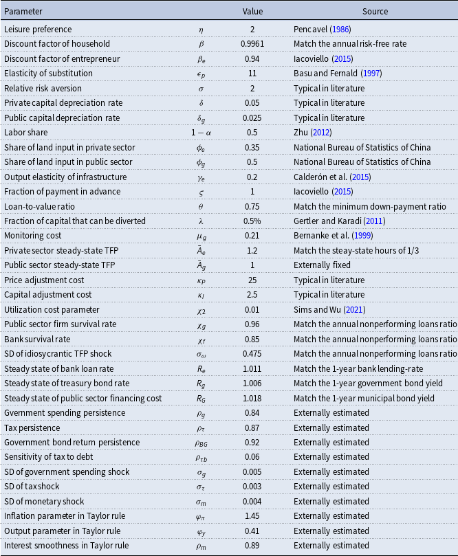
Table 8. Estimated parameters and moments comparison
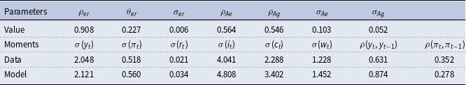
3.3 Impulse responses
Figure 2 illustrates the dynamics of output, consumption, and capital stock and other macroeconomic variables in response to one standard deviation ERS. As shown in Figure 2, ERS leads to a persistent decline of capital stock and a quick decrease in public infrastructure of 0.8%, before infrastructure stock returns to its initial level after 8 quarters. This is because extreme rainfall could directly accelerate the depreciation of capital stock and cause damage to public production facilities. A larger depreciation implies smaller capital inputs both in the public and private sectors, which translates into a significant negative movement of total investment. Consumption also falls persistently, with a maximum drop of over 3% in the first quarter. This is in line with the dynamics of disaster risk documented in the literature (Gourio, Reference Gourio2012; Fernández-Villaverde and Levintal, Reference Fernández-Villaverde and Levintal2018). As disaster events hit the economy, agents will thus become more patient. Their precautionary saving motives increase, and the marginal propensity to consume goes down, and, accordingly, consumption drops. The negative response of inflation rate further corroborates the contraction effects of ERS on aggregate demand.
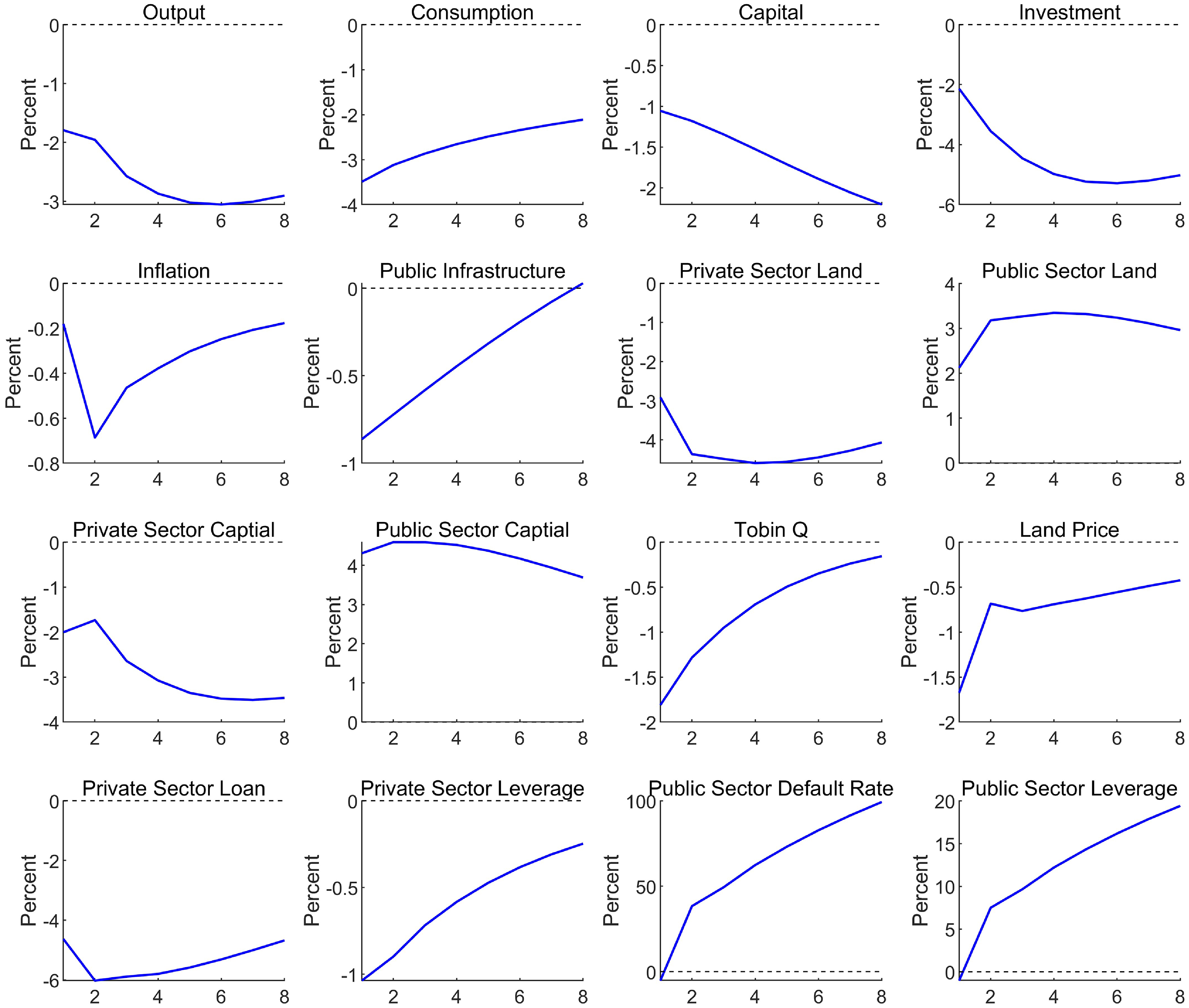
Figure 2. Impulse responses of selected macroeconomic variables to one-standard-deviation extreme rainfall shock.
Notes: Horizontal axes indicate quarters. All responses are in percent.
Figure 2 also shows that both the Tobin Q and land price undergo a significant negative movement, and both reach the lowest level initially (about −1.8% and −1.6%, respectively). The negative responses of Tobin Q and land price induced by ERS suggest that intense precipitation may disrupt the macroeconomy through the financial market. As land price falls and the real estate market struggles, local government’s revenue from land sales drops. The fiscal revenue loss aggravates the fiscal pressure on local governments, and push them to issue more bond to finance their expenditure, to adapt to extreme rainfall events. As we can see from Figure 2, after one SD increase in ERS, the public sector’s leverage displays a positive response within a year, which also results in the rising of default rate in the public sector visible in the figure.
Moreover, private sector loan jumps initially and reaches the lowest level at about −6% in the second quarter. Consequently, firm’s leverage exhibits a sizable negative response within two years. This supports our empirical evidences in the baseline regression. Moreover, the previous section has shown that ERS could adversely affect firm’s leverage through tightening firms’ borrowing constraints or aggravating government debt risk. These channels are also illustrated in Figure 2. On one hand, as extreme precipitation brings about a dip in the real estate market, the declining land price could further harm the financial condition of firms, which would give them less access to bank credit as the value of their collateral land shrinks. On the other hand, extreme rainfall heightens the fiscal pressure of local government, and local governments resort to issuing more debt. Excessive debt burden on local governments transmits default risks to holding banks and further worsens local financing conditions, which will crowd out the bank credit to private sector. The crowding-out effects are also present in the capital and land market. As shown in Figure 2, the capital stock and land in the public sector both show positive responses after the ERS. In contrast, private sector’s inputs of capital and land shrink. This implies that extreme rainfall events will also crowd out the real production resources to private firms.
A deeper insight into the transmission of ERS can be gained by shutting off various features of the model. The consequences for the impulse response to ERS when doing this are shown in Figure 3 and Figure 4, where, for comparison, the impulse response under our baseline parametrization is also reported. We start with the parameter influencing firm’s borrowing constraint, keeping all other parameters at their baseline value.
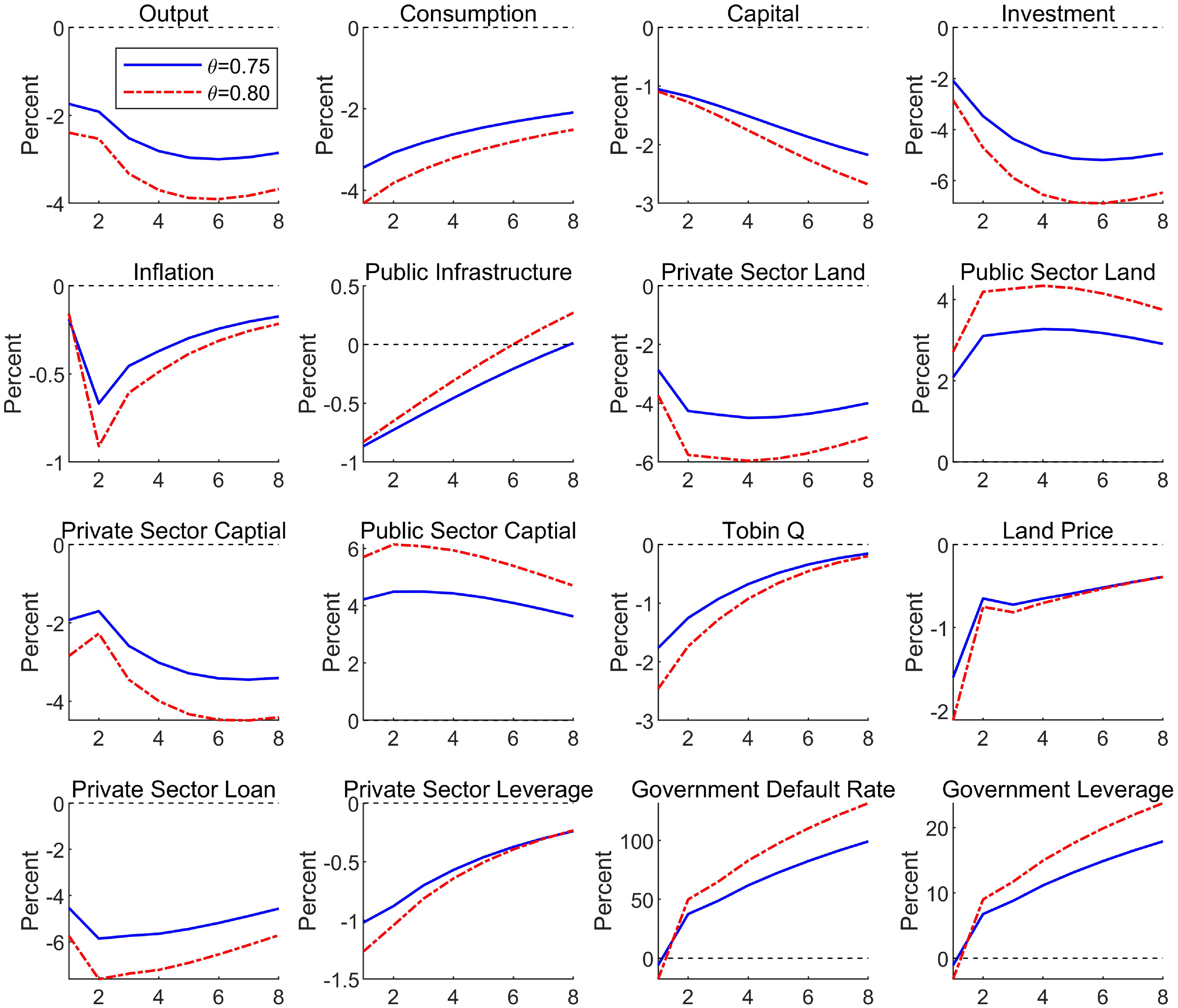
Figure 3. Impulse responses of selected macroeconomic variables to one-standard-deviation extreme rainfall shock when
 $\theta =0.75$
(blue solid line) and
$\theta =0.75$
(blue solid line) and
 $\theta =0.80$
(red dotted line).
$\theta =0.80$
(red dotted line).
Notes: Horizontal axes indicate quarters. All responses are in percent.
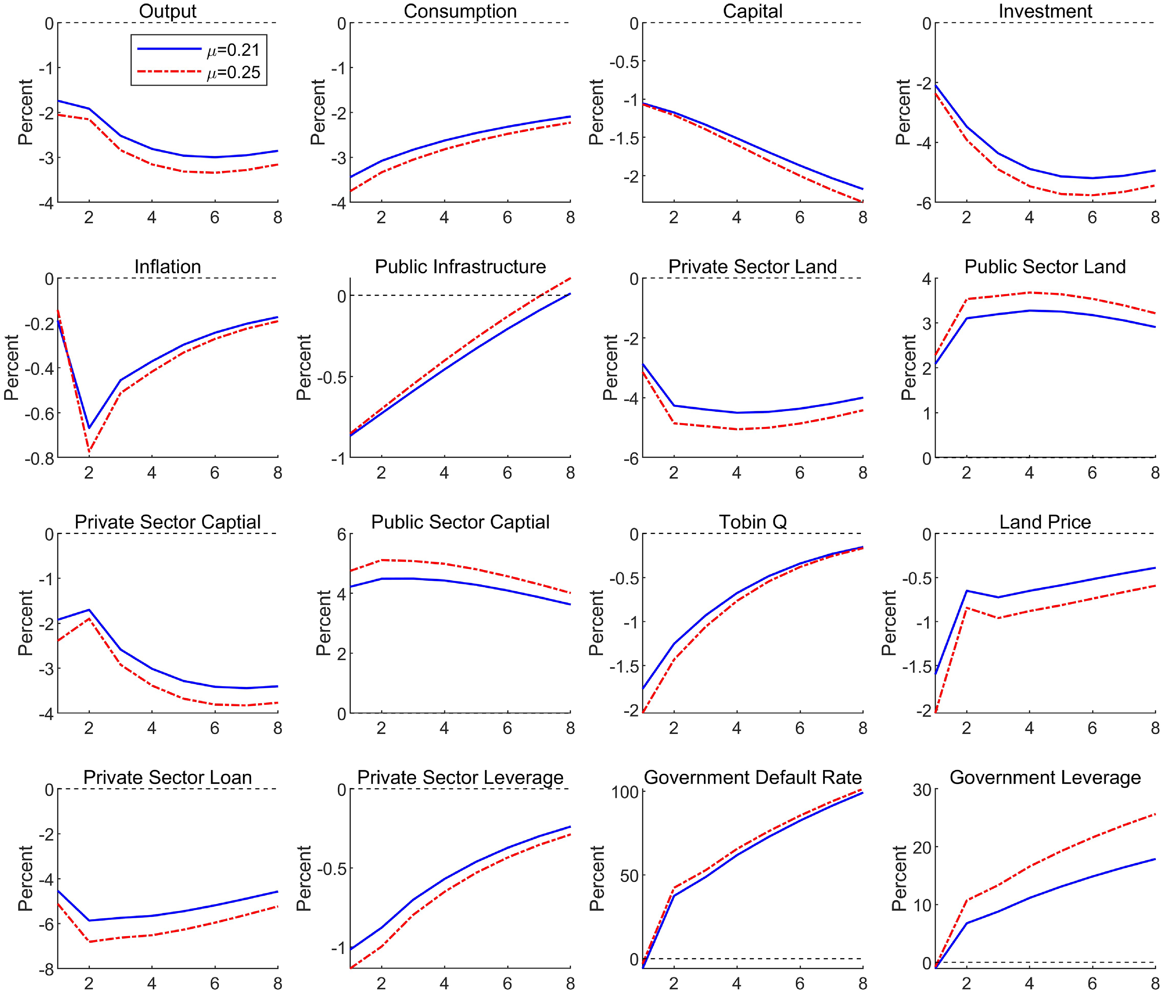
Figure 4. Impulse responses of selected macroeconomic variables to one-standard-deviation extreme rainfall shock when
 $\mu _g=0.21$
(blue solid line) and
$\mu _g=0.21$
(blue solid line) and
 $\mu _g=0.25$
(red dotted line).
$\mu _g=0.25$
(red dotted line).
Notes: Horizontal axes indicate quarters. All responses are in percent.
In Figure 3, we increase the loan-to-value ratio
 $\theta$
from 0.75 to 0.80 to test the aforementioned firms’ balance sheet channel. The larger the loan-to-value ratio, the greater the importance of collateral effects. Higher loan-to-value ratio means that firms’ borrowing capacity is more susceptible to the fluctuations of market value of collateral asset. Therefore, firms’ borrowing constraints would be tighter when the extreme rainfall events trigger declines of asset price in the context of larger loan-to-value ratio. Figure 3 shows that as
$\theta$
from 0.75 to 0.80 to test the aforementioned firms’ balance sheet channel. The larger the loan-to-value ratio, the greater the importance of collateral effects. Higher loan-to-value ratio means that firms’ borrowing capacity is more susceptible to the fluctuations of market value of collateral asset. Therefore, firms’ borrowing constraints would be tighter when the extreme rainfall events trigger declines of asset price in the context of larger loan-to-value ratio. Figure 3 shows that as
 $\theta$
rises, the negative effects of ERS on private sector’s loan and leverage get larger, and the adverse movements of real activities are also amplified. Therefore, firms’ borrowing constraints aggravate the detrimental effects of ERS on firm’s leverage and real economy.
$\theta$
rises, the negative effects of ERS on private sector’s loan and leverage get larger, and the adverse movements of real activities are also amplified. Therefore, firms’ borrowing constraints aggravate the detrimental effects of ERS on firm’s leverage and real economy.
In Figure 4, we shift the monitoring cost parameter
 $\mu _{g}$
from 0.21 to 0.25, all else equal. Higher monitoring cost means more severe financial frictions in the debt market, in which local governments build up higher leverage and afford higher debt financing cost. We find that the higher the monitoring cost, the larger the increase of governments’ leverage, and the stronger the negative effect of ERS on firm’s leverage and real activities. This indicates that government debt risk intensifies the negative impacts of ERS. This result lends strong support to the empirical facts that local government crowding-out effect is a non-negligible channel through which ERS shocks affect firm’s leverage.
$\mu _{g}$
from 0.21 to 0.25, all else equal. Higher monitoring cost means more severe financial frictions in the debt market, in which local governments build up higher leverage and afford higher debt financing cost. We find that the higher the monitoring cost, the larger the increase of governments’ leverage, and the stronger the negative effect of ERS on firm’s leverage and real activities. This indicates that government debt risk intensifies the negative impacts of ERS. This result lends strong support to the empirical facts that local government crowding-out effect is a non-negligible channel through which ERS shocks affect firm’s leverage.
3.4 Welfare analysis
In order to gauge the welfare cost of extreme weather shock, following Schmitt-Grohé and Uribe (Reference Schmitt-Grohé and Uribe2007), we compute the reduction in consumption that households are willing to suffer to completely eliminate the risk of extreme rainfall, that is, by setting the standard deviation of ERS
 $\sigma _{er}$
equal to zero. Specifically, from (2), let
$\sigma _{er}$
equal to zero. Specifically, from (2), let
 $U^{0}$
and
$U^{0}$
and
 $U^{a}$
represent average welfare in baseline model and alternative scenarios, respectively. Then, the welfare loss is implicitly defined by
$U^{a}$
represent average welfare in baseline model and alternative scenarios, respectively. Then, the welfare loss is implicitly defined by
 \begin{align*} U^{a}\left ( \left (1-\omega \right )C_{t}^{a},N_{t}^{a}\right )=U^{0}\left ( C_{t}^{0},N_{t}^{0}\right ), \end{align*}
where
 $\omega \times 100$
represents the percent permanent loss in consumption that should occur in alternative scenarios in order for their households to be as well off as households in baseline case. This welfare metric is standard in the literature of optimal monetary and fiscal policies. Table 6 shows that welfare loss expressed in consumption-equivalent terms, when we change the standard deviation of ERS
$\omega \times 100$
represents the percent permanent loss in consumption that should occur in alternative scenarios in order for their households to be as well off as households in baseline case. This welfare metric is standard in the literature of optimal monetary and fiscal policies. Table 6 shows that welfare loss expressed in consumption-equivalent terms, when we change the standard deviation of ERS
 $\sigma _{er}$
.
$\sigma _{er}$
.
As shown in Table 9, When we change the size of ERS
 $\sigma _{er}$
from 0.01 in the baseline model to 0, it will lead to about 2.18% welfare gain in equivalent terms to consumption.Footnote
10
On the contrary, if we double the size of ERS, this will make the welfare worse than the baseline scenarios as shown in Case 2. In Case 3, we vary the loan-to-value ratio
$\sigma _{er}$
from 0.01 in the baseline model to 0, it will lead to about 2.18% welfare gain in equivalent terms to consumption.Footnote
10
On the contrary, if we double the size of ERS, this will make the welfare worse than the baseline scenarios as shown in Case 2. In Case 3, we vary the loan-to-value ratio
 $\theta$
from 0.75 to 0.80; this will exacerbate firms’ financing conditions when the their collateral assets depreciate and thus lead to welfare loss about 4.07%. In addition, if we increase the monitoring cost parameter from 0.21 to 0.25, the household’s welfare would get worse by −3.62%.
$\theta$
from 0.75 to 0.80; this will exacerbate firms’ financing conditions when the their collateral assets depreciate and thus lead to welfare loss about 4.07%. In addition, if we increase the monitoring cost parameter from 0.21 to 0.25, the household’s welfare would get worse by −3.62%.
Next, we assess the role of government policies in mitigating the effects of extreme rainfall. We will study an augmented Taylor rule whereby the change in the nominal interest rate is set as a function of its own lag, inflation gap, output gap, and extreme rainfall-related events. Formally, this monetary policy rule is given by:
 \begin{align} ln\left (\frac {R_{t}}{\bar {R}}\right ) & =\rho _{m}ln\left (\frac {R_{t-1}}{\bar {R}}\right )+\left (1-\rho _{m}\right )\left (\varphi _{\pi }ln\left (\frac {\pi _{t}}{\bar {\pi }}\right )+\varphi _{y}ln\left (\frac {Y_{t}}{\bar {Y}}\right )-\varphi _{d}er_{t}\right)\nonumber\\& \quad +\varepsilon _{m,t},\varepsilon _{m,t}\sim N\left (0,\sigma _{m}^{2}\right ), \end{align}
where
 $\varphi _{d}$
measures the responsiveness of interest rate to ERS. Given the adverse effects of ERS, we expect that accommodative monetary policy should be implemented to attenuate the detrimental effects of ERS, which implies
$\varphi _{d}$
measures the responsiveness of interest rate to ERS. Given the adverse effects of ERS, we expect that accommodative monetary policy should be implemented to attenuate the detrimental effects of ERS, which implies
 $\varphi _{d}\gt 0.$
Likewise, government spending should be expanded to prevent the economic downturn caused by ERS. This enables us to specify the following fiscal rule:
$\varphi _{d}\gt 0.$
Likewise, government spending should be expanded to prevent the economic downturn caused by ERS. This enables us to specify the following fiscal rule:
 \begin{align} ln\left (\frac {g_{t}}{\bar {g}}\right )=\rho _{g}ln\left (\frac {g_{t-1}}{\bar {g}}\right )+\rho _{gd}er_{t}+\varepsilon _{g,t},\varepsilon _{g,t}\sim N\left (0,\sigma _{g}^{2}\right ), \end{align}
where
 $\rho _{gd}\gt 0$
measures the sensitivity of government spending to ERS. We conduct policy evaluations by computing the welfare variations of the above monetary or fiscal regime relative to the baseline model, where
$\rho _{gd}\gt 0$
measures the sensitivity of government spending to ERS. We conduct policy evaluations by computing the welfare variations of the above monetary or fiscal regime relative to the baseline model, where
 $\varphi _{d}=0$
and
$\varphi _{d}=0$
and
 $\rho _{gd}=0$
.
$\rho _{gd}=0$
.
Table 9. Welfare loss under different scenarios
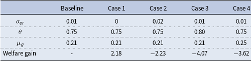
Notes: This table reports the welfare variation expressed in consumption-equivalent terms (%) compared with baseline parameterizations under different scenarios.
We vary the parameter
 $\varphi _{d}\in \left [0,1\right ]$
and
$\varphi _{d}\in \left [0,1\right ]$
and
 $\rho _{gd}\in [0,1]$
, and report the welfare variations in consumption-equivalent terms in Figure 5 and Figure 6, respectively. Figure 5 plots welfare variations as a function of
$\rho _{gd}\in [0,1]$
, and report the welfare variations in consumption-equivalent terms in Figure 5 and Figure 6, respectively. Figure 5 plots welfare variations as a function of
 $\varphi _{d}$
, compare with baseline monetary policy regime. The welfare gains increase monotonically as
$\varphi _{d}$
, compare with baseline monetary policy regime. The welfare gains increase monotonically as
 $\varphi _{d}$
varies from 0 to 1, ranging from 0% to 14%. This implies that central bankers should cut interest rates slightly to mitigate the harmful effects caused by extreme weather disasters.
$\varphi _{d}$
varies from 0 to 1, ranging from 0% to 14%. This implies that central bankers should cut interest rates slightly to mitigate the harmful effects caused by extreme weather disasters.
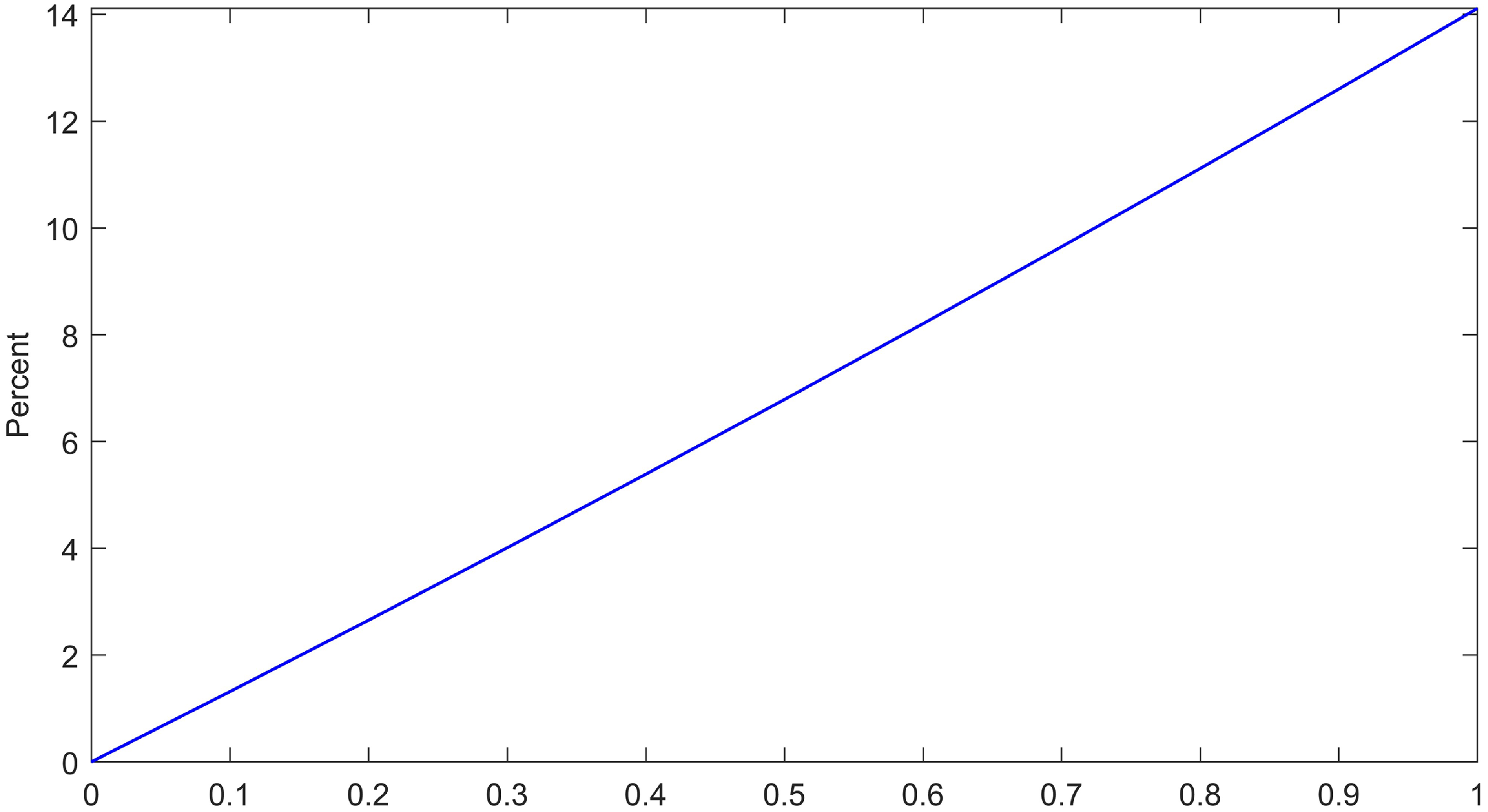
Figure 5. Welfare equivalent consumption variation of different interest rate responsiveness to ERS.

Figure 6. Welfare equivalent consumption variation of different government spending responsiveness to ERS.
As Figure 6 shows, welfare gains are monotonically increasing in
 $\rho _{gd}$
, which indicates that expansionary fiscal policy is conducive to dampening the disaster losses. These findings suggest that accommodating monetary policy and active fiscal policy help to reduce the negative effects of extreme weather events.
$\rho _{gd}$
, which indicates that expansionary fiscal policy is conducive to dampening the disaster losses. These findings suggest that accommodating monetary policy and active fiscal policy help to reduce the negative effects of extreme weather events.
4. Conclusion
China has witnessed a notable increase in the frequency and intensity of extreme precipitation and heavy rainfall in recent years. Motivated by the growing concern about the losses and casualties caused by extreme precipitation, we construct province-level extreme rainfall series based on grids-based meteorological data set in China, and study the impacts of extreme precipitation on corporate leverage. We find that the increase of heavy rainfall would generate a significant decline in firm’s leverage. On the one hand, extreme rainfall would shrink the balance sheet of firm sector and thus tighten the financing conditions, inducing firms to cut down leverage. On the other hand, the concentrated rainfall would aggravate local government debt risk by disturbing the land markets, which would crowd out the credit resources to firm sectors and accelerate their deleveraging. We further build a standard New Keynesian model featuring ERS and financial frictions in the context of China, to elaborate our empirical findings on the transmission of extreme rainfall to corporate leverage. Our model shows that the overall welfare costs of extreme rainfall risk can amount to 2.2% of the agent’s lifetime utility. Additionally, the welfare analysis demonstrates that accommodating monetary policy and active fiscal policy could be employed to mitigate the adverse impacts of extreme precipitation events.
There are several interesting directions to extend the current paper. First, the paper provides empirical evidence for the impacts of extreme precipitation events on individual firms, while intense rainfall will lead to growing pressure on supply chains. The supplier-customer networks of firms might amplify the adverse impacts of extreme weathers, and examine how these connected networks propagate economic losses caused by extreme rainfall would be a fruitful area for further work. Second, our DSGE model neglects the role of macro-prudential policy; extensions to investigating the coordination framework between monetary policy and macro-prudential policy in response to extreme weather shocks may be further investigated. Third, we do not explore the spillover effects of extreme precipitation in the open economy; future research is warranted to better understand the international transmission of extreme weather events.
Supplementary material
The supplementary material for this article can be found at https://doi.org/10.1017/S1365100525100643.
Acknowledgments
We thank the associate editor and the two referees for their suggestions and comments, which helped to significantly improve this paper. Li acknowledges the financial support from the National Natural Science Foundation of China (Grant Number 72103209, 72373074) and the Fundamental Research Funds for the Central Universities (No. 998-63233178). Gong acknowledges the financial support from the Major Project of Philosophy and Social Sciences by the Ministry of Education of China (Grant Number 2023JZDZ025). Wu acknowledges the financial support from the Hunan Provincial Natural Science Foundation of China (Grant Number 2023JJ20019) and the National Social Science Fund of China (Grant Number 72573053). All remaining errors are ours.
Declaration of generative AI and AI-assisted technologies in the writing process
During the preparation of this work, the authors used GPT4.0 developed by OpenAI in order to improve readability and language. After using this tool/service, the authors reviewed and edited the content as needed and take full responsibility for the content of the publication.
Appendix A. Variable definitions and descriptive statistics
A.1 Variable definitions
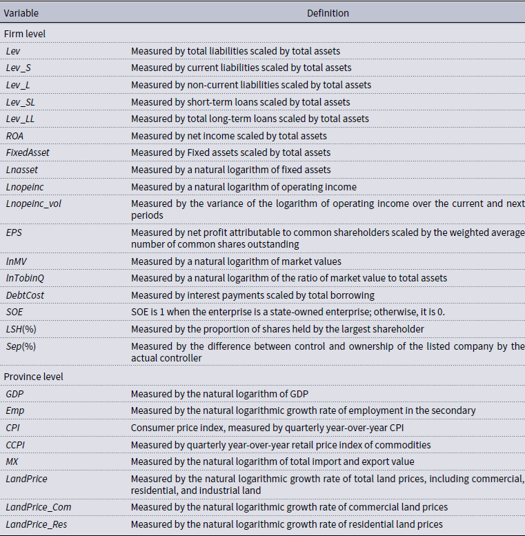
A.2 Descriptive statistics
Table A1 presents the descriptive statistics for the main variables used in our analyses. The standardized extreme rainfall series ranges between −0.80 and 0.78, which indicates that severe rainfall events exhibit a rising trend in some provinces, while other areas may experience a shortage of precipitation. The mean of leverage ratio is 0.4, with a standard deviation of 0.2. As illustrated in Table A1, the average firm has an ROA of 2.7%, a fixed-asset ratio of 20.8% and a basic earnings per share of 0.28 yuan. Within the sample, SOEs account for about 33.5% of firm-quarter observations.
Table A1. Descriptive statistics
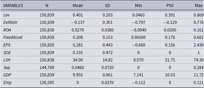
Notes: This table reports descriptive statistics of variables used in this study, including firm-level and province-level variables. The sample of baseline consists of 150,839 quarter-firm observations from 2010 Q1 to 2023 Q3.
Appendix B. Robustness checks
B.1. Dynamic effects of extreme rainfall on firm’s leverage
To investigate the dynamic effects of extreme rainfall on firm’s leverage, we include
 $ExtRain$
with lag periods of 1–4 into the baseline regression and report the estimation results in Table B1. As shown, no matter which lag period of
$ExtRain$
with lag periods of 1–4 into the baseline regression and report the estimation results in Table B1. As shown, no matter which lag period of
 $ExtRain$
is employed, we always find a statistically significant and negative coefficient on
$ExtRain$
is employed, we always find a statistically significant and negative coefficient on
 $ExtRain$
at the 1% level, and the magnitudes are comparable to the baseline case.
$ExtRain$
at the 1% level, and the magnitudes are comparable to the baseline case.
Table B1. Dynamic effects of extreme rainfall on firm’s leverage

Notes: This table reports estimates of the dynamic effects of extreme rainfall on firm’s leverage. Specifically, we replace the independent variable in (1) with extreme rainfall with a lag of 1–4 periods. All lags are included in column (5). The above regressions control for firm-level and province-level control variables, as well as firm and time fixed effects. Cluster-robust standard errors are reported in parentheses clustered at the firm level. See Appendix A.1 for variable definitions. *, **, and *** indicate that the coefficient is significant at the level of 10%, 5%, and 1%.
B.2. Local projection
Furthermore, we examine the dynamic impacts of extreme rainfall on corporate leverage adjustment by employing the local projection (LP) method proposed by Jordà (Reference Jordà2005). The LP approach directly estimates the dynamic response of leverage to an exogenous ERS across multiple horizons, avoiding restrictive assumptions inherent in VAR models. Specifically, for firm
 $i$
at time
$i$
at time
 $t$
, we estimate the following equation for each horizon
$t$
, we estimate the following equation for each horizon
 $h = 0, 1, \ldots , 6$
:
$h = 0, 1, \ldots , 6$
:
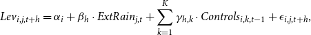 \begin{equation} {Lev}_{i,j,t+h} = \alpha _i + \beta _h \cdot {ExtRain}_{j,t} + \sum _{k=1}^K \gamma _{h,k} \cdot {Controls}_{i,k,t-1} + \epsilon _{i,j,t+h}, \end{equation}
where
 ${Lev}_{i,j,t+h}$
denotes the leverage ratio of firm
${Lev}_{i,j,t+h}$
denotes the leverage ratio of firm
 $i$
in province
$i$
in province
 $j$
at
$j$
at
 $t+h$
, and
$t+h$
, and
 ${ExtRain}_{j,t}$
is the ERS at time
${ExtRain}_{j,t}$
is the ERS at time
 $t$
in province
$t$
in province
 $j$
. The control variables include one-period lagged firm-level characteristics and province-level macroeconomic factors, respectively. Firm fixed effects (
$j$
. The control variables include one-period lagged firm-level characteristics and province-level macroeconomic factors, respectively. Firm fixed effects (
 $\alpha _i$
) account for time-invariant heterogeneity, while the coefficients
$\alpha _i$
) account for time-invariant heterogeneity, while the coefficients
 $\beta _h$
trace the impulse response of leverage to a 1-unit ERS over different periods. Figure 7 in Appendix B presents the dynamic impacts of firms’ leverage in response to extreme rainfall over a 6-quarter horizon, illustrating the persistent negative movement of corporate leverage ratio. These results suggest that the increase of severe rainfall events has a persistent adverse effect on firm’s leverage.
$\beta _h$
trace the impulse response of leverage to a 1-unit ERS over different periods. Figure 7 in Appendix B presents the dynamic impacts of firms’ leverage in response to extreme rainfall over a 6-quarter horizon, illustrating the persistent negative movement of corporate leverage ratio. These results suggest that the increase of severe rainfall events has a persistent adverse effect on firm’s leverage.
B.3. Other measures for corporate leverage
In the baseline regression,
 $Lev$
is calculated as the ratio of firm’s total liability to its total asset. Generally speaking, liabilities are divided into short-term liabilities and long-term liabilities. Current liabilities (also called short-term liabilities) are debts a company must pay within one year, as opposed to long-term liabilities, which are payable beyond 12 months. We thus create two categorized measures for leverage through scaling firm’s short-term and long-term liabilities by its total asset, denoted by
$Lev$
is calculated as the ratio of firm’s total liability to its total asset. Generally speaking, liabilities are divided into short-term liabilities and long-term liabilities. Current liabilities (also called short-term liabilities) are debts a company must pay within one year, as opposed to long-term liabilities, which are payable beyond 12 months. We thus create two categorized measures for leverage through scaling firm’s short-term and long-term liabilities by its total asset, denoted by
 $Lev\_ S$
and
$Lev\_ S$
and
 $Lev\_ L$
, respectively. In addition, we utilize the amount of firm’s short-term and long-term loan scaled by its asset as two alternative proxies (
$Lev\_ L$
, respectively. In addition, we utilize the amount of firm’s short-term and long-term loan scaled by its asset as two alternative proxies (
 $Lev\_ SL$
and
$Lev\_ SL$
and
 $Lev\_ LL$
) for leverage. As shown in Table B2, the coefficients on
$Lev\_ LL$
) for leverage. As shown in Table B2, the coefficients on
 $ExtRain$
are still consistently negative and remain significant except for the case when
$ExtRain$
are still consistently negative and remain significant except for the case when
 $Lev\_ SL$
is employed as the dependent variable. Meanwhile, to address potential scale effects, we implement temporal standardization of firm leverage (column (5)) to complement the cross-sectional standardization. The results remain statistically and economically significant.
$Lev\_ SL$
is employed as the dependent variable. Meanwhile, to address potential scale effects, we implement temporal standardization of firm leverage (column (5)) to complement the cross-sectional standardization. The results remain statistically and economically significant.
Table B2. Robustness tests: other measures for corporate leverage

Notes: This table reports the robust tests of the effects of extreme rainfall on short- and long-term firm’s leverage. The independent variables of columns (1–2) are non-current/current liabilities scaled by total assets. In columns (3–4), we estimate the effect of extreme rainfall on firm’s long-term and short-term loans. In column (5), we standardize firm leverage cross-sectionally. The above regressions control for firm-level and province-level control variables, as well as firm and time fixed effects. Cluster-robust standard errors are reported in parentheses clustered at the firm level. See Appendix A.1 for variable definitions. *, **, and *** indicate that the coefficient is significant at the level of 10%, 5%, and 1%.

Figure 7. Dynamic effects of extreme rainfall on firm’s leverage.
B.4. Other measures for extreme rainfall
We implement a series of adjustments to our measure for extreme rainfall: First, we have reconstructed our extreme rainfall measures at the city level to properly account for intra-provincial climatological variation. We run the baseline regression using the city-level extreme rainfall measures and report the corresponding estimation results in column (1) of Table B3, which confirms the negative movements of corporate leverage adjustments as we observed in the baseline regression. It’s noteworthy to point out that adopting city-level extreme rainfall measure would reduce the sample size remarkably, due to extensive missing meteorological station records across numerous municipalities. Second, we have implemented two additional weighting schemes in constructing extreme rainfall measures, taking account of the geographical area and population size of different cities. To be specific, we utilized the official urban land area data sourced from the China City Statistical Yearbooks and constructed the province-level extreme rainfall indices weighted by constituent cities’ areal proportions (
 $ExtRain\_Area$
). In addition, drawing upon comprehensive demographic records from both the China City Statistical Yearbooks and national population censuses, we developed population-weighted provincial extreme rainfall measures (
$ExtRain\_Area$
). In addition, drawing upon comprehensive demographic records from both the China City Statistical Yearbooks and national population censuses, we developed population-weighted provincial extreme rainfall measures (
 $ExtRain\_Pop$
) using annual city-level resident population figures as weights. The robustness check outcomes displayed in column (2) and column (3) of Table B3 demonstrate virtually identical coefficient magnitudes and statistical significance levels compared to our baseline estimates. These alternative robustness checks collectively provide a more nuanced characterization of precipitation exposures across heterogeneous spatial units while generating qualitatively consistent and statistically significant findings that corroborate our baseline conclusions.
$ExtRain\_Pop$
) using annual city-level resident population figures as weights. The robustness check outcomes displayed in column (2) and column (3) of Table B3 demonstrate virtually identical coefficient magnitudes and statistical significance levels compared to our baseline estimates. These alternative robustness checks collectively provide a more nuanced characterization of precipitation exposures across heterogeneous spatial units while generating qualitatively consistent and statistically significant findings that corroborate our baseline conclusions.
Table B3. Robustness tests: other measures for extreme rainfall
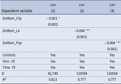
Notes: This table presents robustness checks using alternative measures of
 $ExtRain$
. Column (1) employs one-period-lagged city-level extreme rainfall as the independent variable. It additionally includes “city-year” interaction fixed effects, with standard errors clustered at the city level. Columns (2)–(3) report estimates using province-level extreme rainfall weighted by city land area and population, respectively. The above regressions control for firm-level and province-level control variables, as well as firm and time fixed effects. Cluster-robust standard errors are reported in parentheses clustered at the firm level. See Appendix A.1 for variable definitions. *, **, and *** indicate that the coefficient is significant at the level of 10%, 5%, and 1%.
$ExtRain$
. Column (1) employs one-period-lagged city-level extreme rainfall as the independent variable. It additionally includes “city-year” interaction fixed effects, with standard errors clustered at the city level. Columns (2)–(3) report estimates using province-level extreme rainfall weighted by city land area and population, respectively. The above regressions control for firm-level and province-level control variables, as well as firm and time fixed effects. Cluster-robust standard errors are reported in parentheses clustered at the firm level. See Appendix A.1 for variable definitions. *, **, and *** indicate that the coefficient is significant at the level of 10%, 5%, and 1%.
B.5. Two-stage instrumental variable estimates
Firm location may be endogenous to unobserved risk factors influencing capital structure decisions, such as local industry concentration or pre-existing financing constraints. We implement the instrumental variable (IV) analyses to address this potential endogeneity. Following He et al. (Reference He, Ren, Wang and Lei2025), we employ the length and density of rivers in a firm’s host city as our instruments. The density of river is measured as the length of the river divided by the area of the city. These instruments satisfy both relevance and exclusion conditions: (1) they strongly correlate with local environmental conditions—areas with greater river length/density face higher flood risks and consequently suffer more severe losses when rainfall shocks occur; and (2) being determined by natural geography, river exposure affects corporate leverage only indirectly through influencing regional rainfall and flood risks, rather than directly impacting firms’ balance sheets or capital structure decisions. The two-stage regression results in Table B4 confirm that river characteristics effectively predict extreme rainfall, while extreme rainfall significantly reduces corporate leverage (second stage), thereby robustly supporting our baseline findings.
Table B4. Robustness tests: two-stage instrumental variable estimates
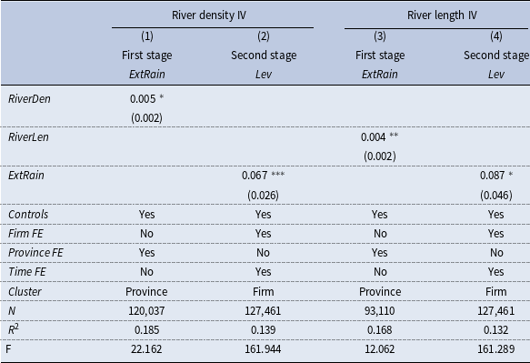
Notes: This table presents two-stage least squares estimates. Columns (1–2) employ city river density as the instrument, measured by the length of the river divided by the area of the city(
 $km/km^{2}$
), while columns (3–4) use city river length (10,000
$km/km^{2}$
), while columns (3–4) use city river length (10,000
 $km$
). All first-stage regressions estimate the impact on
$km$
). All first-stage regressions estimate the impact on
 $ExtRain$
, with second-stage effects on firm leverage (
$ExtRain$
, with second-stage effects on firm leverage (
 $Lev$
). The above regressions control for firm-level and province-level control variables, as well as fixed effects. Cluster-robust standard errors are reported in parentheses. *, **, and *** indicate that the coefficient is significant at the level of 10%, 5%, and 1%.
$Lev$
). The above regressions control for firm-level and province-level control variables, as well as fixed effects. Cluster-robust standard errors are reported in parentheses. *, **, and *** indicate that the coefficient is significant at the level of 10%, 5%, and 1%.