


Impact statement
The passive cooling of buildings with outside air requires sufficiently large ventilation rates driven by a combination of wind and buoyancy effects. Given the complexities of the surrounding urban canopy and the induced flow field, these natural ventilation rates can be highly uncertain and variable. Previous studies have focused either on individual buildings and their surroundings or on very simplified surrounding geometries. This study generalises characteristics from real urban areas into an idealised canopy, considering ventilation through multiple buildings and window configurations. By simulating wind through this canopy along with airflow through building interiors, we highlight the important effect of the surrounding geometry on the local flow field and natural ventilation rates.
1. Introduction
The International Energy Agency has projected that if unchecked, the energy demand for building cooling will triple by 2050. This demand would equal China’s total electricity consumption in 2018 (Dean et al. Reference Dean, Dulac, Morgan and Remme2018), pointing to a global need for more sustainable solutions. One alternative is natural cooling, which requires little or no energy by combining natural ventilation with thermal storage. Natural ventilation uses wind and buoyant forces to drive outside air through a building (Hunt & Linden Reference Hunt and Linden1999). Often, in the evening or at night, these forces exchange cooler outdoor air with warmer indoor air. This outside air cools building surfaces, which function as thermal storage, absorbing heat and maintaining a comfortable indoor temperature during hotter times of the day. Natural cooling systems can replace or augment traditional mechanical cooling, ranging from complex automated systems in larger office buildings (e.g. Stanford’s Y2E2 (Chen & Gorlé Reference Chen and Gorlé2022)) to opportunely opening windows in residential homes. Although predictive tools for indoor and outdoor temperatures have found widespread implementation in recent decades (Zawadzka et al. Reference Zawadzka, Harris and Corstanje2021), characterising wind and interior airflow across the diversity of urban areas remains challenging (Tong et al. Reference Tong, Luo and Zhou2021).
Building energy simulations often represent natural ventilation with one-dimensional (1-D) airflow models (Ramponi et al. Reference Ramponi, Angelotti and Blocken2014). Specified pressures at building openings force these airflow models. Empirical models derived from wind tunnel data often predict these pressures (Orme Reference Orme1999; Cóstola et al. Reference Cóstola, Blocken and Hensen2009). However, wind tunnel data generally span limited building and urban geometries (Freire et al. Reference Freire, Abadie and Mendes2013; Cóstola et al. Reference Cóstola, Blocken and Hensen2009), leading most models to account for surrounding buildings with correction factors that are a function of canopy density (Cóstola et al. Reference Cóstola, Blocken and Hensen2009). While these models are widely used (Chiesa & Grosso Reference Chiesa and Grosso2019; Van Nguyen & De Troyer Reference Van Nguyen and De Troyer2018), they are not broadly accurate (Freire et al. Reference Freire, Abadie and Mendes2013; Ramponi et al. Reference Ramponi, Angelotti and Blocken2014). Additionally, these models do not consider the coupling between the outdoor and indoor airflow.
Large eddy simulation (LES) offers an alternative approach to predict the coupled outdoor and indoor airflow through specific canopy and building geometries. By resolving the larger turbulence scales that dominate the urban canopy and natural ventilation flows, LES can accurately predict the airflow and resulting ventilation rates. Previous LES of coupled indoor and outdoor flow fields often considered idealised building interiors (van Hooff et al. Reference van Hooff, Blocken and Tominaga2017; Hwang & Gorlé Reference Hwang and Gorlé2022b; Hirose et al. Reference Hirose, Ikegaya, Hagishima and Tanimoto2021) and surroundings (Adachi et al. Reference Adachi, Ikegaya, Satonaka and Hagishima2020; King et al. Reference King, Gough, Halios, Barlow, Robertson, Hoxey and Noakes2017), or were building-specific (Hwang & Gorlé Reference Hwang and Gorlé2023; Chen & Gorlé Reference Chen and Gorlé2022). While these studies have supported the validation of LES for wind-driven ventilation, LES can be used more broadly to understand and quantify natural ventilation with a focus on developing models that represent the surrounding urban canopy’s effect.
The objective of this study is to improve our understanding of the impact of urban canopy geometry on wind-driven natural ventilation and cooling under varying wind conditions. To achieve this objective, we use LES to predict wind flow through urban canopy and interior building geometries that intend to represent typical characteristics of real urban geometries. We consider urban canopies consisting of quadrants with changing street orientations at two different densities and calculate the ventilation rates through buildings at different locations within the quadrants for different wind directions. The building interiors include four representative ventilation configurations: cross, corner, dual-room and single-sided. For these four ventilation configurations, we quantify the urban canopy’s effect on natural ventilation flow rates by exploring the impacts of canopy density, wind direction and house location. Through this analysis, we seek to identify the primary factors impacting natural ventilation flow rates in real urban environments. Our results provide a first step towards developing improved models that can efficiently represent the dominant urban canopy effects and support accurate natural ventilation and cooling assessment across large-scale urban areas with diverse geometric characteristics.
Section 2 describes the governing equations, computational set-up and quantification of ventilation rates. Section 3 presents the results both as flow visualisations and ventilation rates, and discusses the implications for future model development. Section 4 summarises the conclusions.
2. Description of computational model and quantities of interest
This section describes the governing equations, computational domain, mesh, boundary conditions and other forcings. Across 16 simulations, we capture the combined effects of canopy density, wind angle, wind speed and indoor–outdoor temperature differences on the interior ventilation rates. We measure ventilation rates through four interior sections with different window configurations.
2.1. Governing equations and numerics
Our simulations use the low-Mach formulation of Cascade Design System’s CharLES solver (Cascade Technologies 2022). CharLES is a finite volume solver with an automated body-fitted meshing technique based on three-dimensional (3-D)-clipped Voronoi diagrams that produces isotropic polyhedral-type cells. Various studies have found good agreement between CharLES and experimental data for natural ventilation and wind pressure loads, including both wind tunnel (Hwang & Gorlé Reference Hwang and Gorlé2022 a; Ciarlatani et al. Reference Ciarlatani, Huang, Philips and Gorlé2023; Vargiemezis & Gorlé Reference Vargiemezis and Gorlé2025) and full-scale data (Hochschild & Gorlé Reference Hochschild and Gorlé2024; Hwang & Gorlé Reference Hwang and Gorlé2023). Many of these studies included complex urban canopies (Hwang & Gorlé Reference Hwang and Gorlé2023; Hochschild & Gorlé Reference Hochschild and Gorlé2024; Vargiemezis & Gorlé Reference Vargiemezis and Gorlé2025).
The low-Mach formulation of CharLES solves the filtered equations for conservation of mass and momentum with the density $\rho$
approximated as the sum of a background density and an isentropic acoustic perturbation. The equations are as follows:
$\rho$
approximated as the sum of a background density and an isentropic acoustic perturbation. The equations are as follows:
 \begin{equation} \frac {\partial \tilde {\rho }}{\partial t} + \frac {\partial \tilde {\rho } \tilde {u}_j}{\partial x_j} = 0, \end{equation}
 \begin{equation} \frac {\partial \tilde {\rho } \tilde {u}_i}{\partial t} + \frac {\partial \tilde {\rho } \tilde {u}_i \tilde {u}_j}{\partial x_j} = - \frac {\partial \tilde {p}}{\partial x_i} + \frac {\partial {\sigma }_{ij}}{\partial x_j}, \end{equation}
 \begin{equation} \tilde {\rho } = \frac {1}{c^2}(\tilde {p} - p_{\text{ref}}) + \rho _{\text{ref}}, \end{equation}
where $\widetilde {(\cdot )}$
denotes LES filtered quantities,
$\widetilde {(\cdot )}$
denotes LES filtered quantities, $u_i$
are the velocity components,
$u_i$
are the velocity components, $p$
is the pressure,
$p$
is the pressure, $\sigma _{ij}$
is the stress tensor,
$\sigma _{ij}$
is the stress tensor, $c$
is the speed of sound,
$c$
is the speed of sound, $p_{\text{ref}}$
is the reference pressure and
$p_{\text{ref}}$
is the reference pressure and $\rho _{\text{ref}}$
is the reference density. The unresolved portion of the stress tensor is modelled with the Vreman subgrid model (Vreman Reference Vreman2004).
$\rho _{\text{ref}}$
is the reference density. The unresolved portion of the stress tensor is modelled with the Vreman subgrid model (Vreman Reference Vreman2004).
The equations are discretised using a second-order backward difference scheme in time and a second-order central discretisation in space. Defining a finite speed of sound results in a lower condition number for the pressure system of equations, which is a Helmholtz equation instead of the Poisson equation that arises in fully incompressible formulations. In the zero Mach number limit, the system will discretely recover an incompressible formulation. Additional insights into the derivation of the Helmholtz system can be found from Ambo et al. (Reference Ambo, Nagaoka, Philips, Ivey, Brés and Bose2020).
2.2. Computational domain and grid
This section begins by describing the urban canopy layouts before detailing the building interiors and computational grid.
2.2.1. Urban canopy layout
Representing the characteristics of real urban canopies is challenging (Adolphe Reference Adolphe2001; Biljecki & Chow Reference Biljecki and Chow2022; Lu et al. Reference Lu, Nazarian, Hart, Krayenhoff and Martilli2023; Xue et al. Reference Xue, Jiang, Liang, Pang, Yabe, Ukkusuri and Ma2022). In this study, we consider an idealised urban area that aims to represent a few key characteristics of real urban canopies. Figure 1 shows the locations of houses across the computational domain. In total, the computational domain includes 140 buildings distributed over four quadrants. Each quadrant contains an identical group of 35 houses that form a five-by-seven staggered grid, with houses staggered in the seven-house direction (along side yards) and aligned in the five-house direction (along streets). Each quadrant is rotated by $90^o$
to define the full domain. The borders between quadrants are equally sized within the domain and across the boundaries.
$90^o$
to define the full domain. The borders between quadrants are equally sized within the domain and across the boundaries.
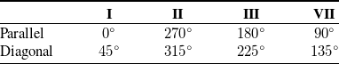
Simulating four quadrants presents a couple of advantages. First, alternating orientations prevent infinitely repeating urban streets, which are not representative of real urban geometries (Lu et al. Reference Lu, Nazarian, Hart, Krayenhoff and Martilli2023). Second, the borders between the four quadrants act as discontinuities, similar to those in real urban layouts, providing greater geometric diversity. In this four-quadrant domain, we run wind directions parallel and diagonal with respect to the urban grid. Across these two simulations, the identical group of 35 houses in each quadrant experiences eight wind directions, as outlined in Table 1. Parallel wind travels along streets in the ${0}^\circ$
and
${0}^\circ$
and ${180}^\circ$
quadrants, and along side yards in the
${180}^\circ$
quadrants, and along side yards in the ${90}^\circ$
and
${90}^\circ$
and ${135}^\circ$
quadrants. Diagonal wind is diagonal to both streets and side yards in all quadrants.
${135}^\circ$
quadrants. Diagonal wind is diagonal to both streets and side yards in all quadrants.
Table 1. Wind angles experienced by each quadrant under wind parallel and diagonal to the urban grid


Figure 1. House placement within the simulation domain. Colours mark interiors across each quadrant.

Figure 2. Canopy horizontal dimensions with $L_R = 4 \text{ m}$
.
$L_R = 4 \text{ m}$
.
We consider two domains representing different canopy densities. The house centres are $50\,\%$
further apart in the low-density domain, but the house dimensions remain the same. Figure 2 shows the horizontal dimensions of both canopies, with the width of the rooms
$50\,\%$
further apart in the low-density domain, but the house dimensions remain the same. Figure 2 shows the horizontal dimensions of both canopies, with the width of the rooms $L_R = 4\text{ m}$
as the reference length. The heights of both domains (
$L_R = 4\text{ m}$
as the reference length. The heights of both domains ( $H$
) are one-third of their lengths.
$H$
) are one-third of their lengths.
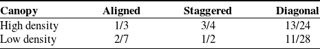
Table 2 summarises the corresponding frontal area fractions ( $\lambda _f$
) of the urban canopies. The frontal area fraction is commonly used to parametrise an urban canopy’s influence on air flow (Wang et al. Reference Wang, Llaguno-Munitxa, Li, Giometto and Bou-Zeid2025; Lu et al. Reference Lu, Nazarian, Hart, Krayenhoff and Martilli2023). Here,
$\lambda _f$
) of the urban canopies. The frontal area fraction is commonly used to parametrise an urban canopy’s influence on air flow (Wang et al. Reference Wang, Llaguno-Munitxa, Li, Giometto and Bou-Zeid2025; Lu et al. Reference Lu, Nazarian, Hart, Krayenhoff and Martilli2023). Here, $\lambda _f$
describes the proportion of the urban area occupied by the urban canopy when looking in the direction of the mean wind. Table 2 presents
$\lambda _f$
describes the proportion of the urban area occupied by the urban canopy when looking in the direction of the mean wind. Table 2 presents $\lambda _f$
along the aligned, staggered and diagonal axes.
$\lambda _f$
along the aligned, staggered and diagonal axes.
Table 2. Frontal area fractions ( $\lambda _f$
) for the urban canopy below
$\lambda _f$
) for the urban canopy below $H_{R}$

2.2.2. Building details
The overall dimensions of each house are 3 $L_R$
by 2
$L_R$
by 2 $L_R$
, with
$L_R$
, with $L_R = 4 \text{ m}$
being the width of interior rooms. The house has a hip roof with a minimum height equal to the interior room height
$L_R = 4 \text{ m}$
being the width of interior rooms. The house has a hip roof with a minimum height equal to the interior room height $H_R = 3\text{ m}$
and a maximum height
$H_R = 3\text{ m}$
and a maximum height $H_H = 2H_{R}$
. The roof features a single ridge extending 2
$H_H = 2H_{R}$
. The roof features a single ridge extending 2 $L_{R}$
over the house centre in the aligned direction. Within each quadrant of 35 houses, six have simulated interiors. While one of the six houses includes skylights, this study focuses on the five houses without skylights, all with identical interiors.
$L_{R}$
over the house centre in the aligned direction. Within each quadrant of 35 houses, six have simulated interiors. While one of the six houses includes skylights, this study focuses on the five houses without skylights, all with identical interiors.
Figure 3 shows the floor plan. The interiors include four separate sections that do not exchange airflow. Three of the sections are individual rooms, while the fourth is two connected rooms. Most rooms are square; the cross-ventilated room is the exception, being $L_{R}$
wide and 2
$L_{R}$
wide and 2 $L_{R}$
long.
$L_{R}$
long.

Figure 3. Floor plan of simulated interiors. Arrows indicate possible ventilation pathlines, with solid arrows showing ventilation axes.
The window placement gives each section a unique ventilation type, as indicated in Figure 3. All windows are $H_{R}/4$
by
$H_{R}/4$
by $H_{R}/4$
. The two rooms in the dual-ventilated section are connected by an open door frame
$H_{R}/4$
. The two rooms in the dual-ventilated section are connected by an open door frame $H_{R}/4$
wide by 3
$H_{R}/4$
wide by 3 $H_{R}/4$
tall. The arrows in Figure 3 trace possible flow paths for each ventilation type. The straight path between two windows will be referred to as the ventilation axes in the remainder of this paper.
$H_{R}/4$
tall. The arrows in Figure 3 trace possible flow paths for each ventilation type. The straight path between two windows will be referred to as the ventilation axes in the remainder of this paper.
2.2.3. Computational grid and time step

Figure 4. Turbulent flow snapshots from parallel and diagonal wind layered over a high density canopy mesh. Plan views at window centre (top) and profile through two quadrant centres (bottom).
Figure 4 shows cross-sections of the mesh created by CharLES’s body-fitted mesh generation based on 3-D-clipped Voronoi diagrams. Each window has five cells across the height and width (Hwang & Gorlé Reference Hwang and Gorlé2022
b), for a mesh resolution of $H_R/20$
. For houses with simulated interiors, this mesh resolution extends for six elements around interior and exterior walls The mesh then coarsens to
$H_R/20$
. For houses with simulated interiors, this mesh resolution extends for six elements around interior and exterior walls The mesh then coarsens to $H_R$
/10 for a distance of
$H_R$
/10 for a distance of $L_R/2$
before coarsening again to
$L_R/2$
before coarsening again to $H_R/5$
, or 10 cells per canopy height. This resolution extends across the adjoining streets to resolve local canopy effects. This mesh resolution also continues through all side yards and within
$H_R/5$
, or 10 cells per canopy height. This resolution extends across the adjoining streets to resolve local canopy effects. This mesh resolution also continues through all side yards and within $L_R$
of houses without simulated interiors. Away from these refinement zones, the mesh size in the canopy is
$L_R$
of houses without simulated interiors. Away from these refinement zones, the mesh size in the canopy is $2H_R/5$
. Moving up from the canopy, the mesh size doubles every five elements, eventually coarsening to
$2H_R/5$
. Moving up from the canopy, the mesh size doubles every five elements, eventually coarsening to $16H_R/5$
. For the high- and low-density canopies, this mesh resolution leads to approximately 9 and 14 million elements, respectively. To check mesh sensitivity, we halved the cell size and simulated the high-density canopy with approximately 53 million elements. This mesh refinement did not significantly change the results, with an average discrepancy of 6 %. Appendix A (included in supplementary material available at https://doi.org/10.1017/flo.2025.10039) shows detailed results for this mesh refinement study. For all simulations, the time step is adjusted to keep the Courant–Friedrichs–Lewy (CFL) condition less than one during the majority of each simulation: 0.02 s for
$16H_R/5$
. For the high- and low-density canopies, this mesh resolution leads to approximately 9 and 14 million elements, respectively. To check mesh sensitivity, we halved the cell size and simulated the high-density canopy with approximately 53 million elements. This mesh refinement did not significantly change the results, with an average discrepancy of 6 %. Appendix A (included in supplementary material available at https://doi.org/10.1017/flo.2025.10039) shows detailed results for this mesh refinement study. For all simulations, the time step is adjusted to keep the Courant–Friedrichs–Lewy (CFL) condition less than one during the majority of each simulation: 0.02 s for $U_{10} = 2\,{\rm m\,s}^{-1}$
and 0.01 s for
$U_{10} = 2\,{\rm m\,s}^{-1}$
and 0.01 s for $U_{10} = 4\,\rm{m\,s}^{-1}$
.
$U_{10} = 4\,\rm{m\,s}^{-1}$
.
2.3. Boundary conditions and periodic forcing
2.3.1. Wind and temperature conditions
The wind speed and temperature conditions used in this study were derived using typical-year weather data from California’s 16 climate zones (California Energy Commission 2022) in combination with a building energy model (BEM). We focus on two cooling scenarios: one in the evening and one at night. For the evening scenario, natural cooling initiates after 4:00 pm as soon as the outdoor temperature drops below the indoor temperature. For the night-time scenario, natural cooling initiates after 11:00 pm if the outdoor temperature is below the indoor temperature. At each ventilation time, we compile wind speeds and indoor–outdoor temperature differences observed in a typical year. Based on this analysis, we selected two typical wind and temperature scenarios: 10 m height wind speeds of 2 and 4 m s−1, and indoor–outdoor temperature differences of 0 and $5\,^\circ\mathrm{C}$
.
$5\,^\circ\mathrm{C}$
.
We performed simulations for the four possible combinations of these conditions, assuming neutral conditions for the outdoor wind flow. This assumption is informed by our focus on evening and night-time ventilation scenarios, but even for a non-neutral outdoor flow, temperature effects can be expected to be relatively small since most ventilation is driven by flow in the isolated roughness regime (Oke Reference Oke1988; Xie et al. Reference Xie, Liu and Leung2007; Xue et al. Reference Xue, Zhao, Mei, Chao and Carmeliet2024). Furthermore, the results presented in this paper only consider ventilation through window openings at a single height, where buoyant effects are small. As a result, we found that the wind speed and indoor–outdoor temperature difference had negligible effects on the non-dimensional velocity and ventilation rates. We therefore average over the set of four simulations for all results in this paper, with each simulation given equal weighting.
2.3.2. Boundary conditions
We represent the top boundary as a slip condition, the horizontal boundary conditions as periodic, and the ground and building surfaces as smooth walls (using a standard algebraic wall model). We found the choice of the wall model (e.g. smooth or rough wall) has a negligible impact on the predicted ventilation rates since the flow is dominated by large-scale sharp-edge separation and wakes. We initialise all surfaces and air volumes with the indoor–outdoor temperature differences from the BEM (see § 2.3.1). The surface temperatures remain fixed while the air volumes mix during the simulation spin-up to a statistically steady-state flow and temperature field.
2.3.3. Periodic wind forcing
A momentum source drives the flow to maintain a constant spatially averaged velocity in the top 10 % of the domain. We assume the velocity near the domain height ( $H$
) reflects an ABL driven by geostrophic wind over a large urban area. Below
$H$
) reflects an ABL driven by geostrophic wind over a large urban area. Below $H$
, local canopy characteristics govern the boundary layer (Letzel et al. Reference Letzel, Krane and Raasch2008; Stull Reference Stull2003). While this local boundary layer depends on the choice of
$H$
, local canopy characteristics govern the boundary layer (Letzel et al. Reference Letzel, Krane and Raasch2008; Stull Reference Stull2003). While this local boundary layer depends on the choice of $H$
, larger
$H$
, larger $H$
values have increasingly smaller effects due to the logarithmic atmospheric boundary layer (ABL) profile (see (2.4)). To set the velocity at
$H$
values have increasingly smaller effects due to the logarithmic atmospheric boundary layer (ABL) profile (see (2.4)). To set the velocity at $H$
, we assume a suburban terrain with bulk roughness
$H$
, we assume a suburban terrain with bulk roughness $y_0 = 0.3$
(Aboshosha et al. Reference Aboshosha, Bitsuamlak and Damatty2015; Stull Reference Stull2003) and disregard the 6 m canopy height, setting the displacement height
$y_0 = 0.3$
(Aboshosha et al. Reference Aboshosha, Bitsuamlak and Damatty2015; Stull Reference Stull2003) and disregard the 6 m canopy height, setting the displacement height $d=0$
for simplicity. We then prescribe a 10 m height wind speed (
$d=0$
for simplicity. We then prescribe a 10 m height wind speed ( $U_{10}$
) and calculate the associated velocity at
$U_{10}$
) and calculate the associated velocity at $H$
using the mean ABL profile
$H$
using the mean ABL profile
 \begin{equation} U(y) = \frac {u_\ast }{\kappa }\ln {\left (\frac {y - d}{y_{0}}\right )}. \end{equation}
We choose the friction velocity ( $u_\ast$
) to yield the desired
$u_\ast$
) to yield the desired $U_{10}$
and set the von Kármán constant to
$U_{10}$
and set the von Kármán constant to $\kappa = 0.41$
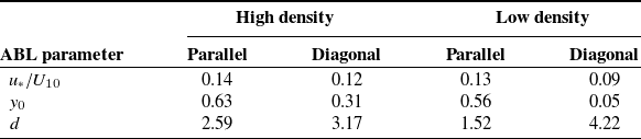
. The simulations initialise from a laminar flow field. Then, as the flow passes through the periodic domain, the boundary layer adjusts to the urban canopy yielding a well-developed turbulent surface layer (Grylls et al. Reference Grylls, Suter and van Reeuwijk2020; Philips et al. Reference Philips, Rossi and Iaccarino2013). Figure 5 shows profiles of mean velocity and turbulence intensities averaged (i) along horizontal domain extents, (ii) over runtime and (iii) across simulations of the four
$\kappa = 0.41$
. The simulations initialise from a laminar flow field. Then, as the flow passes through the periodic domain, the boundary layer adjusts to the urban canopy yielding a well-developed turbulent surface layer (Grylls et al. Reference Grylls, Suter and van Reeuwijk2020; Philips et al. Reference Philips, Rossi and Iaccarino2013). Figure 5 shows profiles of mean velocity and turbulence intensities averaged (i) along horizontal domain extents, (ii) over runtime and (iii) across simulations of the four $U_{10}$
and
$U_{10}$
and $T_{in} - T_{out}$
combinations. Table 3 lists
$T_{in} - T_{out}$
combinations. Table 3 lists $u_\ast$
,
$u_\ast$
, $y_0$
and
$y_0$
and $d$
fit to the mean velocity profiles. These fitted
$d$
fit to the mean velocity profiles. These fitted $y_0$
and
$y_0$
and $d$
show the large effects of canopy density and wind alignment on the resulting boundary layers, with
$d$
show the large effects of canopy density and wind alignment on the resulting boundary layers, with $y_0$
values both above and below the initial
$y_0$
values both above and below the initial $y_0 = 0.3$
estimate.
$y_0 = 0.3$
estimate.

Figure 5. Average profiles of mean velocity ( $U$
) and turbulence intensities (
$U$
) and turbulence intensities ( $I$
), with
$I$
), with $x$
aligned with the mean flow. Lines in the top row show fitted ABL profiles (
$x$
aligned with the mean flow. Lines in the top row show fitted ABL profiles ( $U_{fit}$
), while subsequent lines plot the empirical turbulence intensities using
$U_{fit}$
), while subsequent lines plot the empirical turbulence intensities using $\hat {I_u} \cong 1/\log ((y\!-\!d)/y_0)$
(Holmes Reference Holmes2018). Profiles span the domain height.
$\hat {I_u} \cong 1/\log ((y\!-\!d)/y_0)$
(Holmes Reference Holmes2018). Profiles span the domain height.
Table 3. ABL parameters fit to mean velocities above the canopy

2.4. Summary of LES runs
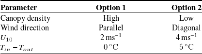
In total, we perform a set of 16 simulations, reflecting all possible combinations of four parameters: canopy density, wind direction, wind speed and indoor–outdoor temperature difference. Table 4 summarises these parameters and their associated values. As mentioned in § 2.3.1, the results presented in this paper were obtained by averaging across different wind speeds and temperature differences, producing four data sets for any given combination of canopy density and wind alignment. Due to the varying quadrant orientation within the domain, the two wind directions (i.e. ‘Parallel’ and ‘Diagonal’) provide data for ventilation rates at eight different wind angles (see § 2.2.1).
Table 4. Parameters varied across LES

The simulations were spun-up over at least four flow passes and subsequently data were collected over at least 18 flow passes. We determined that these spin-up and data collection times were sufficient based on ventilation rate and flow field convergence. On four AMD Epyc 7502 nodes, totalling 128 cores, running a flow-through period for the low-density canopy takes approximately eight hours.
2.5. Quantification of ventilation rates
From the LES time series for the velocity field, we can calculate the instantaneous ventilation rate ( $Q(t)$
) as
$Q(t)$
) as
 \begin{equation} Q(t) = \frac {1}{2}\sum _{i=1}^{N_w} \int _{A_i} \left | \mathbf{u}(t) \cdot \mathbf{n}_i \right | \, \text{d}A, \end{equation}
where, for a given interior space with $N_w$
windows,
$N_w$
windows, $A_i$
is the area of each window and
$A_i$
is the area of each window and $n_i$
is the associated normal vector (Hwang & Gorlé Reference Hwang and Gorlé2022
b). Here,
$n_i$
is the associated normal vector (Hwang & Gorlé Reference Hwang and Gorlé2022
b). Here, $Q$
accounts for turbulent exchange at individual windows by using the absolute values of velocities. The factor of
$Q$
accounts for turbulent exchange at individual windows by using the absolute values of velocities. The factor of $1/2$
prevents double-counting flow into and out of the interior. A time-averaged, non-dimensional ventilation rate is then obtained from
$1/2$
prevents double-counting flow into and out of the interior. A time-averaged, non-dimensional ventilation rate is then obtained from
 \begin{equation} Q_n = \frac {\sum _{i=1}^{N_t}Q(t)}{U_{10} A}, \end{equation}
where $N_t$
is the number of time steps and A is the total window area divided by 2.
$N_t$
is the number of time steps and A is the total window area divided by 2.
To analyse and interpret the variability in the calculated ventilation rates, we use the median and the interquartile range (IQR). The IQR is the distance between the $25\mathrm{th}$
and
$25\mathrm{th}$
and $75\mathrm{th}$
percentiles (
$75\mathrm{th}$
percentiles ( $\text{IQR} = p75 - p25$
), or equivalently the range spanned by the centre 50 % of results when ordered from smallest to largest. We chose the median and IQR because these estimators are interpretable and robust to outliers. To understand the effects of different parameters on ventilation rates, we condition the median and IQR estimates on different parameters. Conditioning on more parameters isolates increasingly specific ventilation scenarios, generally decreasing the IQR. Because this conditioning also reduces the sample size, we report the conditional sample-normalised IQR, defined as
$\text{IQR} = p75 - p25$
), or equivalently the range spanned by the centre 50 % of results when ordered from smallest to largest. We chose the median and IQR because these estimators are interpretable and robust to outliers. To understand the effects of different parameters on ventilation rates, we condition the median and IQR estimates on different parameters. Conditioning on more parameters isolates increasingly specific ventilation scenarios, generally decreasing the IQR. Because this conditioning also reduces the sample size, we report the conditional sample-normalised IQR, defined as
 \begin{equation} \text{IQR}_n(Q_n \mid P_{i:j}) = \text{IQR}(Q_n \mid P_{i:j}) \cdot \Biggr [ \frac {\text{IQR}(Q_n)}{\mathbb{E}_{\text{boot}}[\text{IQR}_n(Q_n)]} \Biggr ], \end{equation}
where $P$
are the parameters specifying the canopy, as reported in Table 4. Dividing
$P$
are the parameters specifying the canopy, as reported in Table 4. Dividing $\text{IQR}(Q_n)$
by
$\text{IQR}(Q_n)$
by $\mathbb{E}_{\text{boot}}[\text{IQR}_n(Q_n)]$
, the bootstrapped estimate of the IQR at that sample size, gives a sample size correction. This correction compares the effect of conditioning on a given parameter with that of randomly selecting a subset of ventilation rates.
$\mathbb{E}_{\text{boot}}[\text{IQR}_n(Q_n)]$
, the bootstrapped estimate of the IQR at that sample size, gives a sample size correction. This correction compares the effect of conditioning on a given parameter with that of randomly selecting a subset of ventilation rates.

Figure 6. Flow fields at window-centre height ( $H/2$
). Keys on the right side show the wind angle (relative to the house) associated with each quadrant in the simulation domain.
$H/2$
). Keys on the right side show the wind angle (relative to the house) associated with each quadrant in the simulation domain.
3. Results and discussion
In this section, we first present visualisations of the mean flow field at two spatial scales: across the full domain and around individual buildings. Next, we quantify ventilation rates and their sensitivity to the parameters listed in Table 4. To explain the ventilation rate sensitivities, we connect ventilation trends with the observed canopy flow characteristics.
3.1. Flow field visualisation
This section first describes qualitatively how the canopy-scale flow depends on (i) canopy density (high versus low), (ii) building alignment (aligned vesus staggered) and (iii) wind direction (parallel versus diagonal). Next, it considers the more local flow field around individual buildings to elucidate how canopy flow effects interact with flow through building interiors. All flow visualisations are at window-centre height ( $H/2$
) and show the normalised velocity (
$H/2$
) and show the normalised velocity ( $U/{U_{10}}$
) averaged across simulations for the two wind speeds and two indoor–outdoor temperature differences (see § 2.3.1).
$U/{U_{10}}$
) averaged across simulations for the two wind speeds and two indoor–outdoor temperature differences (see § 2.3.1).
3.1.1. Domain-scale canopy flow
Figure 6 shows contour plots of the mean velocity magnitude for the two canopy densities, and for parallel and diagonal flow. The plots reveal significant large-scale effects of urban canopy density, building alignment and wind direction on the in-canopy flow.
As expected, the lower density domains support a faster in-canopy flow, consistent with the smaller $\lambda _f$
(see Table 2). This trend also appears between the aligned and staggered quadrants under parallel flow. The aligned quadrants, which have a smaller
$\lambda _f$
(see Table 2). This trend also appears between the aligned and staggered quadrants under parallel flow. The aligned quadrants, which have a smaller $\lambda _f$
, support an overall faster in-canopy flow with the building wakes confined to the smaller side yards. The staggered quadrants cause building wakes to persist through much of the canopy. At the transition between quadrants with different alignments, the overall higher (or lower) velocities from the aligned (or staggered) quadrant persist into the downstream quadrant. Overall, these results show that areas of high
$\lambda _f$
, support an overall faster in-canopy flow with the building wakes confined to the smaller side yards. The staggered quadrants cause building wakes to persist through much of the canopy. At the transition between quadrants with different alignments, the overall higher (or lower) velocities from the aligned (or staggered) quadrant persist into the downstream quadrant. Overall, these results show that areas of high $\lambda _f$
cause reductions in canopy flow velocity which may persist some distance downstream.
$\lambda _f$
cause reductions in canopy flow velocity which may persist some distance downstream.
The diagonal flow cases in Figure 6 also reveal domain-scale variability in wind speed, even though $\lambda _f$
is constant across quadrants. This variation stems from the anisotropic nature of the drag exerted by a quadrant on the flow, i.e. the drag is lower in the direction of the aligned streets. Figure 7 schematically represents the deflection of canopy flow along the streets, as indicated by the arrows in each quadrant. This deflection directs the flow in the canopy to either diverge (orange arrows) or converge (purple arrows), and this diverging/converging pattern sets up a secondary flow pattern. Where the canopy flow diverges, faster flow from above the canopy descends into the canopy, resulting in a higher in-canopy velocity; where the canopy flow converges, slower flow from within the canopy rises and the in-canopy velocity remains lower. The vertical velocities form larger secondary vortices that align with the mean flow direction. Other work has observed these secondary flows over alternating areas of high and low roughness (Anderson et al. Reference Anderson, Barros, Christensen and Awasthi2015; Ma et al. Reference Ma, Xu, Sung, Tian and Huang2025). In summary, the domain-scale flow patterns reveal that both
$\lambda _f$
is constant across quadrants. This variation stems from the anisotropic nature of the drag exerted by a quadrant on the flow, i.e. the drag is lower in the direction of the aligned streets. Figure 7 schematically represents the deflection of canopy flow along the streets, as indicated by the arrows in each quadrant. This deflection directs the flow in the canopy to either diverge (orange arrows) or converge (purple arrows), and this diverging/converging pattern sets up a secondary flow pattern. Where the canopy flow diverges, faster flow from above the canopy descends into the canopy, resulting in a higher in-canopy velocity; where the canopy flow converges, slower flow from within the canopy rises and the in-canopy velocity remains lower. The vertical velocities form larger secondary vortices that align with the mean flow direction. Other work has observed these secondary flows over alternating areas of high and low roughness (Anderson et al. Reference Anderson, Barros, Christensen and Awasthi2015; Ma et al. Reference Ma, Xu, Sung, Tian and Huang2025). In summary, the domain-scale flow patterns reveal that both $\lambda _f$
and anisotropy in the urban canopy drag can cause large-scale variations in wind speed that will impact interior flow and ventilation rates.
$\lambda _f$
and anisotropy in the urban canopy drag can cause large-scale variations in wind speed that will impact interior flow and ventilation rates.

Figure 7. Arrows show diagonal wind projected along streets. The orange arrows show canopy flow divergence (arrows pointing apart), whereas the purple arrows show canopy flow convergence (arrows pointing together). This colouring creates a similar pattern to the diagonal flow field.
3.1.2. Local flow patterns

Figure 8. Mean velocity magnitude at window-centre height for four wind angles. Interiors are located in the centre of their respective quadrant.
Figure 8 shows the time-averaged velocity magnitude around and inside a single house for four wind angles. Lower in-canopy wind speeds in the high-density canopy result in lower flow velocities through window openings. In addition, the interference effects due to surrounding buildings are more significant in the high-density canopy, producing considerably different wind speeds and directions near openings than what would be observed for an isolated building. These changes affect the local momentum and pressure near the openings, which in turn impact ventilation flow.
Considering the ${0}^\circ$
case, the dual- and corner-ventilated rooms have upstream openings that would support significant ventilation flow in the absence of surrounding buildings. However, in the canopy layouts considered in this study, these openings are in the wake of the upstream building and the flow through the openings is small. This effect is larger in the high-density case, which has a skimming flow regime, than in the low-density case, which has an interference flow regime, following the common classification (Hussain & Lee Reference Hussain and Lee1980; Oke Reference Oke1988). A similar effect is observed for the corner- and cross-ventilated rooms under the
${0}^\circ$
case, the dual- and corner-ventilated rooms have upstream openings that would support significant ventilation flow in the absence of surrounding buildings. However, in the canopy layouts considered in this study, these openings are in the wake of the upstream building and the flow through the openings is small. This effect is larger in the high-density case, which has a skimming flow regime, than in the low-density case, which has an interference flow regime, following the common classification (Hussain & Lee Reference Hussain and Lee1980; Oke Reference Oke1988). A similar effect is observed for the corner- and cross-ventilated rooms under the ${90}^\circ$
wind direction. In the high-density canopy, flow rates through window openings are lower, while in the low-density canopy, flow rates are higher due to the larger distance to upstream buildings and wider side yards.
${90}^\circ$
wind direction. In the high-density canopy, flow rates through window openings are lower, while in the low-density canopy, flow rates are higher due to the larger distance to upstream buildings and wider side yards.
For the non-parallel flow directions, we similarly observe important interference effects. In particular, interference effects can significantly alter the local flow direction. For example, in the absence of interference effects, the flow through the corner-ventilated room would be similarly aligned with the ventilation axis for the ${135}^\circ$
and
${135}^\circ$
and ${315}^\circ$
wind directions. However, in the high-density canopy, the surrounding buildings induce changes in the outdoor flow field that yield higher flow rates for the
${315}^\circ$
wind directions. However, in the high-density canopy, the surrounding buildings induce changes in the outdoor flow field that yield higher flow rates for the ${135}^\circ$
wind direction than for the
${135}^\circ$
wind direction than for the ${315}^\circ$
wind direction. In the low-density canopy, this effect is reversed. This example demonstrates that the observed changes in the flow field compared with the flow around an isolated building (see for example Hwang & Gorlé Reference Hwang and Gorlé2022
a) strongly depend on the urban canopy layout. We expect a better representation of these interference effects will be key in improving natural ventilation predictions.
${315}^\circ$
wind direction. In the low-density canopy, this effect is reversed. This example demonstrates that the observed changes in the flow field compared with the flow around an isolated building (see for example Hwang & Gorlé Reference Hwang and Gorlé2022
a) strongly depend on the urban canopy layout. We expect a better representation of these interference effects will be key in improving natural ventilation predictions.
3.2. Ventilation rates
This section presents the ventilation rates and their sensitivity to canopy density, wind direction and house location. We address these parameters from easier to more difficult to characterise. We first discuss the effect of canopy density, which can be described with bulk parameters like $\lambda _f$
and leads to canopy-wide changes in wind speed, as shown in Figure 6. We then address wind angle and house location, which are governed by local canopy flow features.
$\lambda _f$
and leads to canopy-wide changes in wind speed, as shown in Figure 6. We then address wind angle and house location, which are governed by local canopy flow features.
3.2.1. Ventilation rates by room type and overall sensitivity to canopy density
Figure 9 shows the ventilation rate distribution by room type. For each room, the first box plot includes the ventilation rates across all LESs, spanning the parameters outlined in Table 4. These plots show that the dual-room configuration experiences the largest median $Q_n$
at 0.22, followed by the cross (10 % less), corner (35 % less) and single-sided (85 % less) ventilation types. The IQR for dual-room ventilation is approximately 50 % of the median, while the IQR for corner and cross ventilation are approximately 85 % and 90 % of their respective medians. The average IQR across these three rooms is 75 % higher than the difference in ventilation rates between them. This result indicates that, provided there are multiple windows, the ventilation configuration has less impact than the parameters influencing the external flow field.
$Q_n$
at 0.22, followed by the cross (10 % less), corner (35 % less) and single-sided (85 % less) ventilation types. The IQR for dual-room ventilation is approximately 50 % of the median, while the IQR for corner and cross ventilation are approximately 85 % and 90 % of their respective medians. The average IQR across these three rooms is 75 % higher than the difference in ventilation rates between them. This result indicates that, provided there are multiple windows, the ventilation configuration has less impact than the parameters influencing the external flow field.
To quantify the effect of canopy density, the second and third box plots in Figure 9 show each room’s ventilation rate for the high and low canopy densities, respectively. On average, the higher density canopy gives 15 % lower ventilation rates and 40 % lower IQRs. The lower canopy density gives 30 % higher ventilation rates with 20 % higher IQRs. These numbers confirm that a building in a higher density canopy will experience stronger interference effects, where the surrounding canopy geometry starts to dominate the flow and sensitivity to wind angle is reduced. This reduced sensitivity to wind angle will be further explored in § 3.2.2.

Figure 9. Average normalised ventilation through the four room types. For each room, the first box plot shows ventilation rates across all cases while the second two are conditioned on canopy density. Boxes span from the lowest 25th percentile to the upper 75th percentile, with the box length giving the IQR. Whiskers extend 1.5 times the IQR beyond the nearest quartile. Points show ventilation rates beyond this range.

Figure 10. Horizontal lines show the IQR of all $Q_n$
measured in each room, while points show the
$Q_n$
measured in each room, while points show the $\text{IQR}_n$
of
$\text{IQR}_n$
of $Q_n$
conditioned on a parameter subset. In the top row, each
$Q_n$
conditioned on a parameter subset. In the top row, each $\text{IQR}_n$
conditions on a single fixed parameter (
$\text{IQR}_n$
conditions on a single fixed parameter ( $ P_i$
). For example, fixing house location results in five subsets. In the bottom row, each
$ P_i$
). For example, fixing house location results in five subsets. In the bottom row, each $\text{IQR}_n$
conditions on both the given parameter and all preceding parameters on the x-axis (
$\text{IQR}_n$
conditions on both the given parameter and all preceding parameters on the x-axis ( $ P_{1:i}$
), meaning more parameters are progressively fixed. For example, fixing wind angle and density results in 16 subsets.
$ P_{1:i}$
), meaning more parameters are progressively fixed. For example, fixing wind angle and density results in 16 subsets.
To further illustrate the effects of the different parameters, Figure 10 plots the sample-normalised IQRs, or $\text{IQR}_n$
s, for the canopy density, wind angle and house location. The top row provides
$\text{IQR}_n$
s, for the canopy density, wind angle and house location. The top row provides $\text{IQR}_n$
s conditioned on values from a single parameter, showing that the wind angle, followed by the canopy density, has the greatest potential to reduce
$\text{IQR}_n$
s conditioned on values from a single parameter, showing that the wind angle, followed by the canopy density, has the greatest potential to reduce $\text{IQR}_n$
in aggregate. The bottom row of Figure 10 quantifies the joint effect of multiple parameters in aggregate by progressively conditioning
$\text{IQR}_n$
in aggregate. The bottom row of Figure 10 quantifies the joint effect of multiple parameters in aggregate by progressively conditioning $\text{IQR}_n$
s on more parameters. For multi-window ventilation types, conditioning on both density and wind angle provides a significant decrease in
$\text{IQR}_n$
s on more parameters. For multi-window ventilation types, conditioning on both density and wind angle provides a significant decrease in $\text{IQR}_n$
s, showing that natural ventilation models should represent the combined effect of these two parameters to make accurate predictions.
$\text{IQR}_n$
s, showing that natural ventilation models should represent the combined effect of these two parameters to make accurate predictions.
3.2.2. Sensitivity of ventilation rate to wind angle

Figure 11. Ventilation roses with eight primary petals, one for each incident wind direction. These primary petals have five sub-petals, one for each house location, with the average ventilation rate silhouetted behind. The sub-petal colours refer to the relative house locations sketched in the colour key and highlighted in Figure 1. Note the radial axis is 10X smaller for the single-sided ventilation.
Figure 11 shows eight ventilation roses, one for each room configuration and canopy density. These ventilation roses contain eight primary petals, each with five sub-petals. Like wind roses, the primary petals align with the incident wind angle, with their magnitude (outlined behind the sub-petals) indicating the median ventilation rate. The five coloured sub-petals further separate the ventilation by house location, as highlighted by the colour key and Figure 1. The discussion in this section focuses on the primary petals, whereas the sub-petals will be discussed in § 3.2.3.
Figure 11 confirms the previous observation regarding the effect of canopy density; the ventilation rate variability due to wind angle is lower for the high-density canopy than for the low-density canopy. However, the wind angles responsible for above-average ventilation rates are mostly the same between the two canopy densities. These wind angles mostly align with the ventilation axis.
Considering the cross-ventilated room first, the wind roses are symmetric, with ventilation rates mirrored across the axis perpendicular to the ventilation axis ( ${0}^\circ$
and
${0}^\circ$
and ${180}^\circ$
). Higher-than-average ventilation rates are observed for the wind directions that align with the ventilation axis (
${180}^\circ$
). Higher-than-average ventilation rates are observed for the wind directions that align with the ventilation axis ( ${90}^\circ$
and
${90}^\circ$
and ${270}^\circ$
). Similarly, high ventilation rates are observed for the
${270}^\circ$
). Similarly, high ventilation rates are observed for the ${135}^\circ$
and
${135}^\circ$
and ${225}^\circ$
wind directions, where the windows are positioned near the house’s upstream corner, and the wind speed outside is higher than that for the
${225}^\circ$
wind directions, where the windows are positioned near the house’s upstream corner, and the wind speed outside is higher than that for the ${90}^\circ$
and
${90}^\circ$
and ${270}^\circ$
wind directions. In both cases, the flow pattern creates a region of positive stagnation pressure near the inlet window, resulting in higher flow rates. The ventilation rates are significantly lower for wind directions that are perpendicular to the ventilation axis or that place the windows near downstream corners where the pressure assumes a smaller value.
${270}^\circ$
wind directions. In both cases, the flow pattern creates a region of positive stagnation pressure near the inlet window, resulting in higher flow rates. The ventilation rates are significantly lower for wind directions that are perpendicular to the ventilation axis or that place the windows near downstream corners where the pressure assumes a smaller value.
For the corner-ventilated room, the ventilation axis is not aligned with the streets or side yards. As a result, the variability across wind angles becomes more complex, and more pronounced differences between the high- and low-density canopies appear. In the low-density canopy, the angles that coincide with the ventilation axis ( ${135}^\circ$
and
${135}^\circ$
and ${315}^\circ$
) both produce higher-than-average ventilation rates. However, there is a significant difference in the flow rates between the two cases, with the
${315}^\circ$
) both produce higher-than-average ventilation rates. However, there is a significant difference in the flow rates between the two cases, with the ${315}^\circ$
direction providing a 50 % higher ventilation rate than the
${315}^\circ$
direction providing a 50 % higher ventilation rate than the ${135}^\circ$
wind direction. This difference, first noted when discussing the flow patterns in Figure 8, can mostly be attributed to differing interference effects for these two wind angles. In the high-density canopy, the interference effects have the opposite effect, and the ventilation flow rate for the
${135}^\circ$
wind direction. This difference, first noted when discussing the flow patterns in Figure 8, can mostly be attributed to differing interference effects for these two wind angles. In the high-density canopy, the interference effects have the opposite effect, and the ventilation flow rate for the ${315}^\circ$
wind direction is 50 % higher than for the
${315}^\circ$
wind direction is 50 % higher than for the ${135}^\circ$
wind direction. Another notable difference between the high- and low-density canopy is that, in the low-density canopy, the
${135}^\circ$
wind direction. Another notable difference between the high- and low-density canopy is that, in the low-density canopy, the ${90}^\circ$
wind angle produces the highest ventilation rate. In this case, the staggered configuration and wider streets support a higher upstream wind velocity, producing a stronger positive stagnation pressure near the upstream window (see Figure 6).
${90}^\circ$
wind angle produces the highest ventilation rate. In this case, the staggered configuration and wider streets support a higher upstream wind velocity, producing a stronger positive stagnation pressure near the upstream window (see Figure 6).
Finally, the dual-room set-up produces a ventilation rose that is mostly a mirrored version of the corner ventilation rose. This similarity arises because the dual-room geometrically mirrors the corner-ventilated room, with only an additional door opening to the adjacent room. The additional window in the dual-room set-up provides slightly higher ventilation rates across most wind angles, notably for angles where the second room is at the trailing edge of the house with negative relative outdoor pressures.
In summary, the results indicate that alignment of the wind angle with the ventilation axes provides a useful if incomplete indication of effective ventilation directions. Ultimately, ventilation rates depend on the local flow field. This flow field reflects a combination of wind angle and the positions and geometries of surrounding buildings.
3.2.3. Sensitivity of ventilation rates to house location
The five coloured sub-petals in Figure 11 visualise the impact of house location within a quadrant. Across house locations, ventilation rates can vary by up to 60 % of the median in the high-density canopy and 50 % in the low-density canopy. For parallel flow in the high-density canopy, faster flow through the aligned quadrants persists into the first rows of the staggered quadrant. Considering the cross-ventilated room, this faster flow results in higher ventilation rates for the most upstream buildings, i.e. the dark blue petal for ${270}^\circ$
and the light blue petal for
${270}^\circ$
and the light blue petal for ${90}^\circ$
. The corner and dual-room configurations show a similar effect when one of the windows is on the upwind side of the building (
${90}^\circ$
. The corner and dual-room configurations show a similar effect when one of the windows is on the upwind side of the building ( ${90}^\circ$
for the corner and
${90}^\circ$
for the corner and ${270}^\circ$
for the dual-room). In the low-density canopy, this effect is less pronounced. With diagonal wind, the large-scale effect of drag anisotropy and the resulting low- and high-velocity streaks create ventilation differences within each quadrant in both the high- and low-density canopies. This effect is particularly noticeable for the
${270}^\circ$
for the dual-room). In the low-density canopy, this effect is less pronounced. With diagonal wind, the large-scale effect of drag anisotropy and the resulting low- and high-velocity streaks create ventilation differences within each quadrant in both the high- and low-density canopies. This effect is particularly noticeable for the ${45}^\circ$
and
${45}^\circ$
and ${225}^\circ$
winds, where the houses near the edge of the quadrant are located in streaks with higher wind speeds and hence have higher ventilation rates for most ventilation configurations.
${225}^\circ$
winds, where the houses near the edge of the quadrant are located in streaks with higher wind speeds and hence have higher ventilation rates for most ventilation configurations.
The most pronounced deviations in ventilation rate occur for homes near the quadrant edges. While these deviations can be partially explained by the large-scale variations in the flow highlighted above, there are cases (e.g. the dual-room set-up at 225 $^\circ$
) in which local differences in the canopy geometry upstream or downstream of the edge buildings play a dominant role. The variations in geometry produce local differences in wind direction and wind speed, and we expect that they are common in real urban geometries that have a higher degree of non-uniformity.
$^\circ$
) in which local differences in the canopy geometry upstream or downstream of the edge buildings play a dominant role. The variations in geometry produce local differences in wind direction and wind speed, and we expect that they are common in real urban geometries that have a higher degree of non-uniformity.
3.3. Implications for natural ventilation modelling
Models for natural ventilation typically determine wind-driven airflow rates based on the pressure differences that drive the flow. These models typically rely on empirical relationships or user-defined inputs for pressure coefficients at window openings (DOE 2025). These empirical relationships were derived from wind tunnel experiments on isolated rectangular-shaped buildings. If applied, the corrections for interference effects are in the form of a single correction coefficient. For example, Energy Plus’s only ventilation model that accounts for a surrounding canopy requires a user-specified shelter class, as defined in the ASHRAE fundamentals handbook. Based on this shelter class, a single factor reduces all wind-driven flow rates (ASHRAE 2017; DOE 2025; Swami & Chandra Reference Swami and Chandra1988).
The results presented in Figure 9 confirm that, on aggregate, a higher density canopy results in lower ventilation rates. This aggregate observation might seem to support the current approach of applying a factor that reduces ventilation rates for higher density canopies, but the more detailed results presented in Figure 11 indicate that this method does not accurately capture the interference effects that arise in real urban canopies. Changes in flow rates between different canopy densities depend on both the wind angle and surrounding building geometries. Furthermore, different street orientations and related changes in drag introduce large-scale variability in wind speed and direction within a canopy of a given density. The dependency of these local and large-scale effects on specific urban geometry poses a significant modelling challenge given the diverse geometrical configurations in realistic urban areas. To improve accuracy, natural ventilation models must represent both the local and larger-scale effects of a specific urban canopy geometry. Neither of these effects relates well to a single scaling factor applied to the pressure coefficients for an isolated building. Performing large-scale LES for every building designed to use natural ventilation will be out of reach for the foreseeable future, but there is an opportunity to explore the creation of large representative databases that can inform improved modelling strategies and support the training of data-driven models.
4. Conclusion
This study explored the impact of the urban canopy on wind-driven natural ventilation across four ventilation configurations: cross, corner, dual-room and single-sided. We performed LES of coupled indoor/outdoor airflow for two canopy densities and varying wind directions. By analysing the results, we identified the dominant factors that impact natural ventilation flow rates in realistic urban environments.
Flow field visualisations revealed different flow patterns that can affect ventilation rates. At domain-scale, in-canopy variability of wind speeds was observed due to varying $\lambda _f$
and drag anisotropy. Higher
$\lambda _f$
and drag anisotropy. Higher $\lambda _f$
slows down canopy flow, while anisotropic canopy drag creates high- and low-velocity streaks. At a more local scale, interference effects from specific canopy elements can significantly alter the ventilation flow into buildings. When adjacent buildings are directly upstream of a window, the wind speed available for ventilation is often significantly reduced. In other scenarios, surrounding buildings can induce local changes in wind angle and wind speed. These changes often reduce ventilation rates but can also increase them by creating more favourable wind angles or amplifying local velocities.
$\lambda _f$
slows down canopy flow, while anisotropic canopy drag creates high- and low-velocity streaks. At a more local scale, interference effects from specific canopy elements can significantly alter the ventilation flow into buildings. When adjacent buildings are directly upstream of a window, the wind speed available for ventilation is often significantly reduced. In other scenarios, surrounding buildings can induce local changes in wind angle and wind speed. These changes often reduce ventilation rates but can also increase them by creating more favourable wind angles or amplifying local velocities.
The measured ventilation rates reinforced the effects observed in the flow field visualisations. Median ventilation rates differ by 35 % across multi-window ventilation configurations (cross, corner and dual-sided), but changes in the surrounding flow field result in significantly more variability in the ventilation rates (50 %–85 %). For the higher canopy density (with higher $\lambda _f$
), the overall reduction in wind speed resulted in 15 % reduced ventilation rates compared with the median. In addition, the flow field has to align more strongly with the streets and side yards, reducing sensitivity to wind angle. Wind angles that align with a room’s ventilation axis or place one window on the upwind side of the building often drive high ventilation rates. In both cases, the inflow window is likely to be located in a high-pressure stagnation region, whereas the outflow window will be in a lower pressure region. However, as observed in the flow field visualisations, interference effects from surrounding buildings can play an equally important role in determining ventilation rates for specific wind angles. The importance of the specific configuration of surrounding buildings was further highlighted by considering the ventilation rates obtained in houses near quadrant edges. In certain cases, unique interference effects alter the ventilation rate by up to 60 % compared with houses in quadrant centres. To a lesser extent, the domain-scale effects of varying
$\lambda _f$
), the overall reduction in wind speed resulted in 15 % reduced ventilation rates compared with the median. In addition, the flow field has to align more strongly with the streets and side yards, reducing sensitivity to wind angle. Wind angles that align with a room’s ventilation axis or place one window on the upwind side of the building often drive high ventilation rates. In both cases, the inflow window is likely to be located in a high-pressure stagnation region, whereas the outflow window will be in a lower pressure region. However, as observed in the flow field visualisations, interference effects from surrounding buildings can play an equally important role in determining ventilation rates for specific wind angles. The importance of the specific configuration of surrounding buildings was further highlighted by considering the ventilation rates obtained in houses near quadrant edges. In certain cases, unique interference effects alter the ventilation rate by up to 60 % compared with houses in quadrant centres. To a lesser extent, the domain-scale effects of varying $\lambda _f$
and drag anisotropy also cause different ventilation rates across houses within a quadrant.
$\lambda _f$
and drag anisotropy also cause different ventilation rates across houses within a quadrant.
In summary, this study reveals a nuanced interaction between urban canopy geometry and wind angle, which combine to determine the effectiveness of different natural ventilation configurations. Existing models used for the design and analysis of naturally ventilated buildings do not accurately represent these interactions, resulting in significant uncertainty when predicting ventilation rates in new or existing buildings. Future work should focus on developing new models that can better represent these geometry-specific canopy effects to accurately assess natural ventilation and cooling at larger scales. The LES data presented in this paper can provide a starting point for developing such models. Further simulations could explore buoyancy-driven ventilation with openings at different heights, such as skylights, as well as non-neutral boundary layer conditions.
Supplementary material
The supplementary material for this article can be found at https://doi.org/10.1017/flo.2025.10039.
Acknowledgements
Computing for this project was performed on the Sherlock cluster. We would like to thank Stanford University and the Stanford Research Computing Center for providing computational resources and support that contributed to these research results.
Data availability statement
Raw data are available at https://doi.org/10.25740/vb900bf9392 and from the corresponding author (N.B.).
Author contributions
N.B. and C.G. created the research plan. N.B. performed all simulations and data analysis. C.G. and H.S. contributed guidance and advice during the research process. N.B. wrote the manuscript, which H.S. and C.G. reviewed and edited.
Funding statement
C.G. gratefully acknowledges funding by a gift from Autodesk Research and Stanford’s Strategic Energy Research Consortium.
Competing interests
The authors declare no conflict of interest.
Ethical statement
The research meets all ethical guidelines, including adherence to the legal requirements of the study country.


 Open access