


1 Introduction
Categorical variables, which share the same category classification, appear in various fields, including medicine, education, and social science, and have long been the subject of analysis. A table derived from the combination of the variables is known as a square contingency table. Numerous studies have analyzed contingency tables and evaluated the independence or association between variables, but recently, new methods have been proposed by Chatterjee (Reference Chatterjee2021), Forcina & Kateri (Reference Forcina and Kateri2021), Kateri (Reference Kateri2018), and Urasaki et al. (Reference Urasaki, Nakagawa, Momozaki and Tomizawa2024). In the square contingency table, the observed values are concentrated in the diagonal components and tend to decrease as they move away from the diagonal components. This feature clearly shows a strong association, making traditional analysis methods inappropriate. Therefore, research has increasingly focused on symmetry and the transition between variables has advanced in the context of square contingency table analysis. It is important to investigate how similar or transitional the variables are between the two-time points or cohorts, and explore the departure from symmetry is also of interest.
There are two well-known methodological approaches to the analysis of symmetry: model and measure. As for models, in addition to the symmetry test (Bowker, Reference Bowker1948), referred to as the symmetry (S) model in Goodman (Reference Goodman1979) and Agresti (Reference Agresti2010), the marginal homogeneity (MH) model (Stuart, Reference Stuart1955) and the quasi symmetry (QS) model (Caussinus, Reference Caussinus1965) are well known, as are the recently proposed models with divergence by Kateri (Reference Kateri2021) and Tahata (Reference Tahata2022). The measure approach evaluates the degree of departure from the models within a fixed interval regardless of sample size. These features enable the quantification and comparison of the degrees of departure from the model for each contingency table observed across various factors, including confounding issues. As an example, Tomizawa et al. (Reference Tomizawa, Seo and Yamamoto1998) proposed a generalized divergence-type measure that guarantees that the degree of departure from the S model can be evaluated in the range of 0 to 1 by a power-divergence. (For more details on power-divergence statistics, see Cressie & Read (Reference Cressie and Read1984), Read & Cressie (Reference Read and Cressie1988).)
While many methods have been proposed to understand the overall structure of contingency tables, a method to understand the relationships among categories through visualization has existed for a long. This is called correspondence analysis (CA), proposed by Benzécri, which has aided the realization of sophisticated and easy-to-understand visualizations, enabling quick interpretation and understanding of data. Simple CA is still widely used and easily implemented using tools, such as SAS, R, and Python. It is a visualization based on Pearson’s chi-square statistic, described in detail by Beh & Lombardo (Reference Beh and Lombardo2014) and Greenacre (Reference Greenacre2017). Visualization based on the approximations of power-divergence statistics has also been proposed by Beh & Lombardo (Reference Beh and Lombardo2024b). Many proposals aim to understand relationships among categories of the contingency table based on independence or association evaluation methods. However, visualizations focusing on departures from symmetry have been proposed by Beh & Lombardo (Reference Beh and Lombardo2022, Reference Beh and Lombardo2024a), Greenacre (Reference Greenacre2000), and Van der Heijden et al. (Reference Van der Heijden, De Falguerolles and De Leeuw1989). In particular, Greenacre (Reference Greenacre2000) and Van der Heijden et al. (Reference Van der Heijden, De Falguerolles and De Leeuw1989) provide a visualization approach based on singular value decomposition (SVD) applied to the skew-symmetric matrix $\mathbf N$
, which is obtained as the residual matrix between the asymmetric square matrix of observed proportions
$\mathbf N$
, which is obtained as the residual matrix between the asymmetric square matrix of observed proportions $\mathbf P$
and the proportion matrix
$\mathbf P$
and the proportion matrix $\mathbf M$
under the S model. Several studies have applied the SVD approach with Constantine & Gower (Reference Constantine and Gower1978) and Tomizawa & Murata (Reference Tomizawa and Murata1992) serving as examples. Similarly, Beh & Lombardo (Reference Beh and Lombardo2022, Reference Beh and Lombardo2024a) also provide a visualization based on the SVD approach to a skew-symmetric matrix, but uses a skew-symmetric matrix derived from residuals based on power-divergence statistics. These proposals, which utilize the residuals, have the advantage of treating the power-divergence statistic as an index of departure from symmetry. Additionally, the principal coordinates and singular values obtained through the SVD can be directly linked to the statistic, allowing for a more concise and interpretable discussion.
$\mathbf M$
under the S model. Several studies have applied the SVD approach with Constantine & Gower (Reference Constantine and Gower1978) and Tomizawa & Murata (Reference Tomizawa and Murata1992) serving as examples. Similarly, Beh & Lombardo (Reference Beh and Lombardo2022, Reference Beh and Lombardo2024a) also provide a visualization based on the SVD approach to a skew-symmetric matrix, but uses a skew-symmetric matrix derived from residuals based on power-divergence statistics. These proposals, which utilize the residuals, have the advantage of treating the power-divergence statistic as an index of departure from symmetry. Additionally, the principal coordinates and singular values obtained through the SVD can be directly linked to the statistic, allowing for a more concise and interpretable discussion.
In this study, we propose a methodological approach to visually provide the relationship between nominal categories based on the degree of departure from symmetry by the modified power-divergence statistics in two-way square contingency tables. This study, similar to Beh & Lombardo (Reference Beh and Lombardo2024a), provides a visualization of departures from symmetry based on the SVD of a residual matrix derived from power-divergence statistics. However, our proposal, which employs the modified power-divergence statistics, offers several advantages. A particularly significant advantage is that the scaling of departures from symmetry, quantified by Tomizawa et al.’s measure, is independent of sample size. This allows for meaningful comparisons and unification of CA plots across square contingency tables with different sample sizes. A detailed discussion on this point, including an analysis using two real datasets with different sample sizes, is provided in Section 6. Furthermore, unlike Beh & Lombardo (Reference Beh and Lombardo2024a), our approach avoids the second-order Taylor series approximation of power-divergence statistics and provides an exact CA framework without relying on approximations. We discuss the characteristics of CA in the context of symmetry about Tomizawa et al.’s measure, the construction of confidence regions for each category in the CA plot, and applications to real data. These contributions are expected to offer new insights into symmetry.
2 Analysis of symmetry
Consider an $R\times R$
contingency table with nominal categories for the row variable X and the column variable Y. Let
$R\times R$
contingency table with nominal categories for the row variable X and the column variable Y. Let $p_{ij}$
denote the probability that an observation will fall in the ith row and jth column of the table (
$p_{ij}$
denote the probability that an observation will fall in the ith row and jth column of the table ( $i=1,\ldots , R;j=1,\ldots , R)$
. Let
$i=1,\ldots , R;j=1,\ldots , R)$
. Let $p_{i\cdot }=\sum _{j=1}^R p_{ij}$
and
$p_{i\cdot }=\sum _{j=1}^R p_{ij}$
and $p_{\cdot j}=\sum _{i=1}^R p_{ij}$
denote the marginal probabilities. Conversely, let
$p_{\cdot j}=\sum _{i=1}^R p_{ij}$
denote the marginal probabilities. Conversely, let $n_{ij}$
denote the observed frequency in the ith row and jth column of the table. The totals
$n_{ij}$
denote the observed frequency in the ith row and jth column of the table. The totals $n_{i\cdot }$
,
$n_{i\cdot }$
, $n_{\cdot j}$
, and n are also denoted as
$n_{\cdot j}$
, and n are also denoted as $n_{i\cdot }=\sum _{j=1}^R n_{ij}$
,
$n_{i\cdot }=\sum _{j=1}^R n_{ij}$
, $n_{\cdot j}=\sum _{i=1}^R n_{ij}$
, and
$n_{\cdot j}=\sum _{i=1}^R n_{ij}$
, and $n = \sum _{i=1}^R\sum _{j=1}^R n_{ij}$
, respectively. Furthermore, when analyzing symmetry using real data, it is common to assume a multinomial distribution for the
$n = \sum _{i=1}^R\sum _{j=1}^R n_{ij}$
, respectively. Furthermore, when analyzing symmetry using real data, it is common to assume a multinomial distribution for the $R\times R$
contingency table and to replace the cell probabilities
$R\times R$
contingency table and to replace the cell probabilities $p_{ij}$
with their estimates
$p_{ij}$
with their estimates $\hat {p}_{ij}=n_{ij}/n$
. Using this notation, we introduce Bowker’s test and Tomizawa et al.’s measure.
$\hat {p}_{ij}=n_{ij}/n$
. Using this notation, we introduce Bowker’s test and Tomizawa et al.’s measure.
2.1 Bowker’s test statistic
Bowker’s test, for symmetry, may be undertaken by defining the S model with
 $$ \begin{align*} H_0 \: : \: p_{ij} = p_{ji}; \; \forall i, j. \end{align*} $$
Under the null hypothesis $H_0$
, Bowker’s
$H_0$
, Bowker’s $\chi ^2$
statistics is presented as follows:
$\chi ^2$
statistics is presented as follows:
 $$ \begin{align*} \chi^2_{S} &= \frac{1}{2}\sum^R_{i=1}\sum^R_{j=1}\frac{(n_{ij}-n_{ji})^2}{n_{ij}+ n_{ji}} \\ &= \mathop{\sum}^R_{i < j}\frac{(n_{ij}-n_{ji})^2}{n_{ij}+n_{ji}}. \end{align*} $$
It follows a chi-squared distribution with $R(R-1)/2$
degrees of freedom.
$R(R-1)/2$
degrees of freedom. $H_0$
is rejected for high values of
$H_0$
is rejected for high values of $\chi ^2_{S}$
. Bowker’s test is a generalization of McNemar’s test (McNemar, Reference McNemar1947) for an
$\chi ^2_{S}$
. Bowker’s test is a generalization of McNemar’s test (McNemar, Reference McNemar1947) for an $R\times R$
contingency table with
$R\times R$
contingency table with $R>2$
. Beh & Lombardo (Reference Beh and Lombardo2022) proposed a visualization of the degree of departures from symmetry based on
$R>2$
. Beh & Lombardo (Reference Beh and Lombardo2022) proposed a visualization of the degree of departures from symmetry based on $\chi ^2_S/n$
.
$\chi ^2_S/n$
.
2.2 Tomizawa et al.’s power-divergence-type measure
When the S model does not hold by Bowker’s test, one can quantitatively evaluate the degree of departure from symmetry. In particular, Tomizawa et al. (Reference Tomizawa, Seo and Yamamoto1998) proposed the following power-divergence-type measure $\Phi ^{(\lambda )}$
based on the power-divergence, to quantify departures from symmetry:
$\Phi ^{(\lambda )}$
based on the power-divergence, to quantify departures from symmetry:
 $$ \begin{align*} \Phi^{(\lambda)} = \frac{\lambda(\lambda+1)}{2^\lambda-1}I^{(\lambda)}\left(\{{p}^{\ast}_{ij};{p}^{s}_{ij}\} \right), \quad \lambda> -1, \end{align*} $$
where
 $$ \begin{align*} I^{(\lambda)}\left(\{{p}^{\ast}_{ij};{p}^{s}_{ij}\} \right) = \frac{1}{\lambda(\lambda+1)} \sum^R_{i=1}\sum^R_{\substack{j=1 \\ i \neq j}}{p}^{\ast}_{ij}\left[ \left( \frac{{p}^{\ast}_{ij}}{{p}^{s}_{ij}}\right)^{\lambda} - 1 \right]. \end{align*} $$
Assume that $\{{p}_{ij}+{p}_{ji}\}$
for
$\{{p}_{ij}+{p}_{ji}\}$
for $i\neq j$
are all positive, and
$i\neq j$
are all positive, and ${p}^{\ast}_{ij}$
and
${p}^{\ast}_{ij}$
and ${p}^s_{ij}$
are defined as
${p}^s_{ij}$
are defined as ${p}^{\ast}_{ij}={p}_{ij}/{\delta }$
and
${p}^{\ast}_{ij}={p}_{ij}/{\delta }$
and ${p}^s_{ij}=({p}^{\ast}_{ij} + {p}^{\ast}_{ji})/2$
, with
${p}^s_{ij}=({p}^{\ast}_{ij} + {p}^{\ast}_{ji})/2$
, with ${\delta } = \sum ^R_{i=1}\sum ^R_{\substack {j=1 \\ i \neq j}} {p}_{ij}$
. An interesting aspect of this measure,
${\delta } = \sum ^R_{i=1}\sum ^R_{\substack {j=1 \\ i \neq j}} {p}_{ij}$
. An interesting aspect of this measure, ${\Phi }^{(\lambda )}$
, is that it utilizes the conditional probability
${\Phi }^{(\lambda )}$
, is that it utilizes the conditional probability ${p}^{\ast}_{ij}={p}_{ij}/\delta $
instead of
${p}^{\ast}_{ij}={p}_{ij}/\delta $
instead of ${p}_{ij}$
. This represents the probability of an observation falling into the (
${p}_{ij}$
. This represents the probability of an observation falling into the ( $i,j$
) cell since it does not fall into the main diagonal cells. In the analysis of square contingency tables, the symmetry model does not impose any constraints on the cell probabilities along the main diagonal of the table. Therefore, Tomizawa (Reference Tomizawa1994) proposed Pearson and KL divergence-type measures to quantify the departure from symmetry under the condition that an observation falls into a cell other than those on the main diagonal. As a result, the conditional probability
$i,j$
) cell since it does not fall into the main diagonal cells. In the analysis of square contingency tables, the symmetry model does not impose any constraints on the cell probabilities along the main diagonal of the table. Therefore, Tomizawa (Reference Tomizawa1994) proposed Pearson and KL divergence-type measures to quantify the departure from symmetry under the condition that an observation falls into a cell other than those on the main diagonal. As a result, the conditional probability ${p}^{\ast}_{ij}={p}_{ij}/{\delta }$
was directly used instead of
${p}^{\ast}_{ij}={p}_{ij}/{\delta }$
was directly used instead of ${p}_{ij}$
. Furthermore,
${p}_{ij}$
. Furthermore, ${\Phi }^{(\lambda )}$
, proposed in Tomizawa et al. (Reference Tomizawa, Seo and Yamamoto1998), serves as a generalization of the measures introduced in Tomizawa (Reference Tomizawa1994). Consequently, it adopts
${\Phi }^{(\lambda )}$
, proposed in Tomizawa et al. (Reference Tomizawa, Seo and Yamamoto1998), serves as a generalization of the measures introduced in Tomizawa (Reference Tomizawa1994). Consequently, it adopts ${p}^{\ast}_{ij}={p}_{ij}/{\delta }$
in its formulation.
${p}^{\ast}_{ij}={p}_{ij}/{\delta }$
in its formulation.
The measure ${\Phi }^{(\lambda )}$
shares the following three properties for
${\Phi }^{(\lambda )}$
shares the following three properties for $\lambda> -1$
, similar to those of
$\lambda> -1$
, similar to those of $\Phi ^{(\lambda )}$
described in Tomizawa et al. (Reference Tomizawa, Seo and Yamamoto1998). Additionally, the parameter
$\Phi ^{(\lambda )}$
described in Tomizawa et al. (Reference Tomizawa, Seo and Yamamoto1998). Additionally, the parameter $\lambda $
is determined by the user, and the case of
$\lambda $
is determined by the user, and the case of $\lambda \rightarrow 0$
is treated as
$\lambda \rightarrow 0$
is treated as $\lambda = 0$
.
$\lambda = 0$
.
Theorem 2.1. The ${\Phi }^{(\lambda )}$
satisfies the following properties for all
${\Phi }^{(\lambda )}$
satisfies the following properties for all $\lambda $
:
$\lambda $
:
-
1. ${\Phi }^{(\lambda )}$
must lie between 0 and 1.
${\Phi }^{(\lambda )}$
must lie between 0 and 1. -
2.
${\Phi }^{(\lambda )} = 0$
if and only if there is a complete structure of symmetry, that is,
${p}_{ij}={p}_{ji}$
. -
3.
${\Phi }^{(\lambda )} = 1$
if and only if there is a structure in which the degree of departure of symmetry is the largest, that is,
${p}_{ij} = 0$
(then
${p}_{ji}> 0$
) or
${p}_{ji} = 0$
(then
${p}_{ij}> 0$
).


When analyzing real data using the measure, the estimated value of Tomizawa et al.’s power-divergence-type measure, $\hat {\Phi }^{(\lambda )}$
, is calculated using the plug-in estimators
$\hat {\Phi }^{(\lambda )}$
, is calculated using the plug-in estimators $\delta $
,
$\delta $
, $p^{\ast}_{ij}$
, and
$p^{\ast}_{ij}$
, and $p^{s}_{ij}$
, where
$p^{s}_{ij}$
, where $p_{ij}$
is replaced by
$p_{ij}$
is replaced by $\hat {p}_{ij}=n_{ij}/n$
. We refer to
$\hat {p}_{ij}=n_{ij}/n$
. We refer to $\hat {\Phi }^{(\lambda )}$
as the modified power-divergence statistics, because it is derived by normalizing the power-divergence statistics for symmetry such that its maximum value is
$\hat {\Phi }^{(\lambda )}$
as the modified power-divergence statistics, because it is derived by normalizing the power-divergence statistics for symmetry such that its maximum value is $1$
. In particular, when
$1$
. In particular, when $\lambda = - 1/2$
,
$\lambda = - 1/2$
, $0$
,
$0$
, $2/3$
, and
$2/3$
, and $1$
, the plug-in estimator
$1$
, the plug-in estimator $\hat {\Phi }^{(\lambda )}$
relates to famous divergence statistics with a special name, called Freeman–Tukey statistic, KL divergence statistic (log-likelihood statistic), Cressie–Read statistic, and Pearson’s divergence statistic, respectively. However, note that the measure by Tomizawa et al. (Reference Tomizawa, Seo and Yamamoto1998) is defined only for
$\hat {\Phi }^{(\lambda )}$
relates to famous divergence statistics with a special name, called Freeman–Tukey statistic, KL divergence statistic (log-likelihood statistic), Cressie–Read statistic, and Pearson’s divergence statistic, respectively. However, note that the measure by Tomizawa et al. (Reference Tomizawa, Seo and Yamamoto1998) is defined only for $\lambda> -1$
to ensure that its values remain between 0 and 1. Therefore, as a limitation, some important divergence statistics, such as the reverse KL divergence statistic (
$\lambda> -1$
to ensure that its values remain between 0 and 1. Therefore, as a limitation, some important divergence statistics, such as the reverse KL divergence statistic ( $\lambda = -1$
) and the reverse Pearson’s divergence statistic (
$\lambda = -1$
) and the reverse Pearson’s divergence statistic ( $\lambda = -2$
), cannot be applied. The relationship between the values of the power-divergence statistic proposed by Cressie & Read (Reference Cressie and Read1984) and the estimates of the measure is detailed in Section 6 (Concluding Remarks) of Tomizawa et al. (Reference Tomizawa, Seo and Yamamoto1998).
$\lambda = -2$
), cannot be applied. The relationship between the values of the power-divergence statistic proposed by Cressie & Read (Reference Cressie and Read1984) and the estimates of the measure is detailed in Section 6 (Concluding Remarks) of Tomizawa et al. (Reference Tomizawa, Seo and Yamamoto1998).
The important point in this Section 2.2 is that the sample size n does not appear in the estimator $\hat {\Phi }^{(\lambda )}$
. Therefore, the major benefit of the estimator
$\hat {\Phi }^{(\lambda )}$
. Therefore, the major benefit of the estimator $\hat {\Phi }^{(\lambda )}$
is that it can be quantified independently of the sample size, making it suitable for comparing the asymmetry of multiple contingency tables. While the
$\hat {\Phi }^{(\lambda )}$
is that it can be quantified independently of the sample size, making it suitable for comparing the asymmetry of multiple contingency tables. While the $\hat {\Phi }^{(\lambda )}$
may seem a simple modification of the power-divergence statistic of Cressie & Read (Reference Cressie and Read1984) due to the adjustment by
$\hat {\Phi }^{(\lambda )}$
may seem a simple modification of the power-divergence statistic of Cressie & Read (Reference Cressie and Read1984) due to the adjustment by $\hat {\delta }$
, its properties are significantly different, and this distinction is notable. Additionally, to ensure that the
$\hat {\delta }$
, its properties are significantly different, and this distinction is notable. Additionally, to ensure that the $\hat {\Phi }^{(\lambda )}$
takes values between 0 and 1 independently on the sample size, the parameter is constrained by
$\hat {\Phi }^{(\lambda )}$
takes values between 0 and 1 independently on the sample size, the parameter is constrained by $\lambda> -1$
. Simple CA based on the estimator
$\lambda> -1$
. Simple CA based on the estimator $\hat {\Phi }^{(\lambda )}$
retains the same advantages and limitations, specifically its independence of sample size and the need to constrain the parameter
$\hat {\Phi }^{(\lambda )}$
retains the same advantages and limitations, specifically its independence of sample size and the need to constrain the parameter $\lambda $
within a specific range to maintain this property.
$\lambda $
within a specific range to maintain this property.
3 Visualization and modified power-divergence statistics in simple CA
Visualization of relationships between categories in contingency tables enables rapid interpretation and understanding of data, even for non-experts. In particular, when examining the symmetry of nominal categories, it is important to analyze the similar or transitional relationship of categories between two-time points or cohorts. This section shows that the modified power-divergence statistics can be used to visualize the symmetric structures and interrelationships of individual categories.
3.1 SVD of matrices by modified power-divergence statistics
The estimator $\hat {\Phi }^{(\lambda )}$
(and the measure
$\hat {\Phi }^{(\lambda )}$
(and the measure $\Phi ^{(\lambda )}$
) can also be defined as
$\Phi ^{(\lambda )}$
) can also be defined as
 $$ \begin{align*} \hat{\Phi}^{(\lambda)} &= \sum^R_{i=1}\sum^R_{\substack{j=1 \\ i \neq j}}\frac{\hat{p}^{\ast}_{ij}+\hat{p}^{\ast}_{ji}}{2}\left[1- \frac{\lambda 2^\lambda}{2^\lambda-1}\hat{H}^{(\lambda)}_{ij}(\{\hat{p}^{c}_{ij},\hat{p}^{c}_{ji}\}) \right] = \sum^R_{i=1}\sum^R_{\substack{j=1 \\ i \neq j}} \hat{\phi}^{(\lambda)}_{ij}, \end{align*} $$
where
 $$ \begin{align*} \hat{H}^{(\lambda)}_{ij}(\{\hat{p}^{c}_{ij},\hat{p}^{c}_{ji}\}) &= \frac{1}{\lambda} \left[1-(\hat{p}^{c}_{ij})^{\lambda+1} - (\hat{p}^{c}_{ji})^{\lambda+1} \right], \\\hat\phi^{(\lambda)}_{ij} &= \frac{\hat{p}^{\ast}_{ij}+\hat{p}^{\ast}_{ji}}{2}\left[1- \frac{\lambda 2^\lambda}{2^\lambda-1}\hat{H}^{(\lambda)}_{ij}(\{\hat{p}^{c}_{ij},\hat{p}^{c}_{ji}\}) \right], \end{align*} $$
and $\hat {p}^{c}_{ij} = \hat {p}_{ij}/(\hat {p}_{ij}+\hat {p}_{ji})$
. The estimator
$\hat {p}^{c}_{ij} = \hat {p}_{ij}/(\hat {p}_{ij}+\hat {p}_{ji})$
. The estimator $\hat {\phi }^{(\lambda )}_{ij}$
estimates a partial measure that quantifies the departure from symmetry for each (
$\hat {\phi }^{(\lambda )}_{ij}$
estimates a partial measure that quantifies the departure from symmetry for each ( $i, j$
) cell of the contingency table and is non-negative. Let us consider the
$i, j$
) cell of the contingency table and is non-negative. Let us consider the $R\times R$
matrix
$R\times R$
matrix $\mathbf S_{skew(\lambda )}$
, constructed from the estimator
$\mathbf S_{skew(\lambda )}$
, constructed from the estimator $\hat {\Phi }^{(\lambda )}$
, with zero diagonal elements and the following (
$\hat {\Phi }^{(\lambda )}$
, with zero diagonal elements and the following ( $i, j$
) elements:
$i, j$
) elements:
 $$ \begin{align*} s_{ij} = \left\{ \begin{array}{@{}cr@{}} \text{sign}(\hat{p}_{ij}-\hat{p}_{ji}) \sqrt{\hat{\phi}^{(\lambda)}_{ij}} & (i \neq j), \\ 0 & (i = j), \end{array} \right. \end{align*} $$
where $\text {sign}(x)$
is a sign function defined as follows:
$\text {sign}(x)$
is a sign function defined as follows:
 $$ \begin{align*} \text{sign}(x) = \left\{ \begin{array}{@{}rl@{}} 1 & (x> 0),\\ 0 & (x = 0), \\ -1 & ( x < 0). \end{array} \right. \end{align*} $$
The matrix with such elements is called an anti-symmetric or skew-symmetric matrix, and $\mathbf S_{skew(\lambda )}^T=- \mathbf S_{skew(\lambda )}$
. The matrix
$\mathbf S_{skew(\lambda )}^T=- \mathbf S_{skew(\lambda )}$
. The matrix $\mathbf S_{skew(\lambda )}$
can also be interpreted as a residual matrix derived from the modified power-divergence statistic, scaled by the
$\mathbf S_{skew(\lambda )}$
can also be interpreted as a residual matrix derived from the modified power-divergence statistic, scaled by the $\hat {\Phi }^{(\lambda )}$
to ensure that it is not affected by sample size. Moreover, when the contingency table exhibits perfect symmetry, the matrix becomes a zero matrix. If symmetry exists only for certain categories, all elements in the rows and columns corresponding to those categories are zero. Using this matrix, the
$\hat {\Phi }^{(\lambda )}$
to ensure that it is not affected by sample size. Moreover, when the contingency table exhibits perfect symmetry, the matrix becomes a zero matrix. If symmetry exists only for certain categories, all elements in the rows and columns corresponding to those categories are zero. Using this matrix, the $\hat {\Phi }^{(\lambda )}$
can be expressed as
$\hat {\Phi }^{(\lambda )}$
can be expressed as
 $$ \begin{align*} \hat{\Phi}^{(\lambda)} &= \sum^R_{i=1}\sum^R_{\substack{j=1 \\ i \neq j}} \hat{\phi}^{(\lambda)}_{ij} \\ &= trace(\mathbf S_{skew(\lambda)}^T \mathbf S_{skew(\lambda)}) \\ &= trace(\mathbf S_{skew(\lambda)} \mathbf S_{skew(\lambda)}^T). \end{align*} $$
It indicates that $\mathbf S_{skew(\lambda )}$
can reconstruct the
$\mathbf S_{skew(\lambda )}$
can reconstruct the $\hat {\Phi }^{(\lambda )}$
with information about the degree of departure from symmetry for each cell. The fact that such reconstruction is possible implies that, as discussed in Section 3.3, the total inertia in this study can be represented by
$\hat {\Phi }^{(\lambda )}$
with information about the degree of departure from symmetry for each cell. The fact that such reconstruction is possible implies that, as discussed in Section 3.3, the total inertia in this study can be represented by $\hat {\Phi }^{(\lambda )}$
, just as in a standard simple CA where the total inertia is expressed as
$\hat {\Phi }^{(\lambda )}$
, just as in a standard simple CA where the total inertia is expressed as $\chi ^2 / n $
using the chi-square test statistic
$\chi ^2 / n $
using the chi-square test statistic $\chi ^2$
.
$\chi ^2$
.
To visualize departures from symmetry, the matrices representing the principal coordinates of the row and column categories are obtained from the SVD of $\mathbf S_{skew(\lambda )}$
, that is,
$\mathbf S_{skew(\lambda )}$
, that is,
 $$ \begin{align*} \mathbf S_{skew(\lambda)} &= \mathbf A\mathbf D_{\mu}\mathbf B^T, \end{align*} $$
where $\mathbf A$
and
$\mathbf A$
and $\mathbf B$
are
$\mathbf B$
are $R\times M$
orthogonal matrices containing left and right singular vectors of
$R\times M$
orthogonal matrices containing left and right singular vectors of $\mathbf S_{skew(\lambda )}$
, respectively, and
$\mathbf S_{skew(\lambda )}$
, respectively, and $\mathbf D_\mu $
is
$\mathbf D_\mu $
is $M\times M$
diagonal matrix with singular values
$M\times M$
diagonal matrix with singular values $\mu _m$
(
$\mu _m$
( $m =1,\dots , M$
). The singular values
$m =1,\dots , M$
). The singular values $\mu _m$
are also lined up in consecutive pairs of values, so that
$\mu _m$
are also lined up in consecutive pairs of values, so that $1>\mu _1 = \mu _2 > \mu _3 = \mu _4 > \dots \geq 0$
. Since
$1>\mu _1 = \mu _2 > \mu _3 = \mu _4 > \dots \geq 0$
. Since $\mathbf S_{skew(\lambda )}$
is a skew-symmetric matrix, M varies depending on the number of categories. Therefore,
$\mathbf S_{skew(\lambda )}$
is a skew-symmetric matrix, M varies depending on the number of categories. Therefore,
 $$ \begin{align*} M = \begin{cases} R, & R \text{ is even}, \\ R-1, & R \text{ is odd}. \end{cases} \end{align*} $$
The SVD of the skew-symmetric matrix $\mathbf S_{skew (\lambda )}$
can also be expressed as
$\mathbf S_{skew (\lambda )}$
can also be expressed as
 $$ \begin{align*} \mathbf S_{skew(\lambda)} &= \mathbf A\mathbf D_{\mu}\mathbf J_M \mathbf A^T, \end{align*} $$
where
 $$ \begin{align*} \mathbf B &= \mathbf A\mathbf J_M^T. \end{align*} $$ $\mathbf J_M$
is a block diagonal and orthogonal skew-symmetric matrix made up of
$\mathbf J_M$
is a block diagonal and orthogonal skew-symmetric matrix made up of $2\times 2$
blocks
$2\times 2$
blocks
 $$ \begin{align*} \mathbf J_2 &= \begin{pmatrix} 0 & 1 \\ -1 & 0 \end{pmatrix}. \end{align*} $$
If R is odd, the matrix has a 0 in the final position. For a detailed description of features of the skew-symmetric matrix, see Gower (Reference Gower1977).
3.2 Principal coordinates and their characteristics
To obtain the principal coordinates of row and column categories using these matrices $\mathbf A$
,
$\mathbf A$
, $\mathbf B$
, and
$\mathbf B$
, and $\mathbf D_\mu $
in the case of symmetry, we propose row and column coordinate matrices expressed as
$\mathbf D_\mu $
in the case of symmetry, we propose row and column coordinate matrices expressed as $\mathbf F$
and
$\mathbf F$
and $\mathbf G$
, respectively, defined as
$\mathbf G$
, respectively, defined as
 $$ \begin{align*} \begin{cases} \mathbf F = \mathbf A\mathbf D_{\mu}, \\ \mathbf G = \mathbf B\mathbf D_{\mu}. \end{cases} \end{align*} $$
When defining $\mathbf D_r$
and
$\mathbf D_r$
and $\mathbf D_c$
as diagonal matrices with
$\mathbf D_c$
as diagonal matrices with $\hat {p}_{i\cdot }$
and
$\hat {p}_{i\cdot }$
and $\hat {p}_{\cdot j}$
as their diagonal elements, the metric matrix
$\hat {p}_{\cdot j}$
as their diagonal elements, the metric matrix $\mathbf D = (\mathbf D_r + \mathbf D_c)/2$
, used in Greenacre (Reference Greenacre2000) and Beh & Lombardo (Reference Beh and Lombardo2022, Reference Beh and Lombardo2024a), is not used in the construction of
$\mathbf D = (\mathbf D_r + \mathbf D_c)/2$
, used in Greenacre (Reference Greenacre2000) and Beh & Lombardo (Reference Beh and Lombardo2022, Reference Beh and Lombardo2024a), is not used in the construction of $\mathbf F$
and
$\mathbf F$
and $\mathbf G$
in this study. Note that the elements
$\mathbf G$
in this study. Note that the elements $s_{ij}$
of
$s_{ij}$
of $\mathbf S_{skew(\lambda )}$
can be expressed in the following form based on the matrices
$\mathbf S_{skew(\lambda )}$
can be expressed in the following form based on the matrices $\mathbf A$
and
$\mathbf A$
and $\mathbf D_{\mu }$
obtained via the SVD of
$\mathbf D_{\mu }$
obtained via the SVD of $\mathbf S_{skew(\lambda )}$
:
$\mathbf S_{skew(\lambda )}$
:
 $$ \begin{align*} s_{ij} \risingdotseq \mu_1 (a_{i1}a_{j2} - a_{j1}a_{i2}), \end{align*} $$
where $a_{im}$
is the (
$a_{im}$
is the ( $i, m$
)th element of
$i, m$
)th element of $\mathbf A$
. From the above, the element
$\mathbf A$
. From the above, the element $s_{ij}$
is given in terms of a triangle formed by the origin and the coordinate pairs of categories (
$s_{ij}$
is given in terms of a triangle formed by the origin and the coordinate pairs of categories ( $a_{i1}, a_{i2}$
) and (
$a_{i1}, a_{i2}$
) and ( $a_{j1}, a_{j2}$
). The expression
$a_{j1}, a_{j2}$
). The expression $a_{i1}a_{j2} - a_{j1}a_{i2}$
can be either positive or negative values. A positive value indicates that
$a_{i1}a_{j2} - a_{j1}a_{i2}$
can be either positive or negative values. A positive value indicates that $(a_{i1}, a_{i2})$
is positioned clockwise related to
$(a_{i1}, a_{i2})$
is positioned clockwise related to $(a_{j1}, a_{j2})$
, while a negative value indicates a counterclockwise position. When
$(a_{j1}, a_{j2})$
, while a negative value indicates a counterclockwise position. When $s_{ij}=0$
and
$s_{ij}=0$
and $a_{i1}a_{j2} - a_{j1}a_{i2}$
approaches zero,
$a_{i1}a_{j2} - a_{j1}a_{i2}$
approaches zero, $(a_{i1}, a_{i2})$
,
$(a_{i1}, a_{i2})$
, $(a_{j1}, a_{j2})$
, and the origin appear to be collinear, though not perfectly aligned. If the area of the triangle is large, it can be interpreted as a greater departure from symmetry between category i and category j. The approach of using areas to visually represent asymmetry has been proposed in Corcuera & Giummolé (Reference Corcuera and Giummolé1998) and Chino (Reference Chino1990) and is considered an effective method. Focusing on this property, when the (
$(a_{j1}, a_{j2})$
, and the origin appear to be collinear, though not perfectly aligned. If the area of the triangle is large, it can be interpreted as a greater departure from symmetry between category i and category j. The approach of using areas to visually represent asymmetry has been proposed in Corcuera & Giummolé (Reference Corcuera and Giummolé1998) and Chino (Reference Chino1990) and is considered an effective method. Focusing on this property, when the ( $i, m$
)th element
$i, m$
)th element $f_{im}$
is defined as the row coordinate matrix
$f_{im}$
is defined as the row coordinate matrix $\mathbf F$
, the area of the triangle formed by the two-dimensional coordinates of the ith and jth row categories,
$\mathbf F$
, the area of the triangle formed by the two-dimensional coordinates of the ith and jth row categories, $(f_{i1}, f_{i2})$
and
$(f_{i1}, f_{i2})$
and $(f_{j1}, f_{j2})$
, along with the origin, is given as
$(f_{j1}, f_{j2})$
, along with the origin, is given as
 $$ \begin{align*} f_{i1}f_{j2} - f_{j1}f_{i2} = \mu^2_1 (a_{i1}a_{j2} - a_{j1}a_{i2}) \risingdotseq \mu_1 s_{ij}. \end{align*} $$
Although the overall area is scaled by $\mu _1$
due to the absence of the metric
$\mu _1$
due to the absence of the metric $\mathbf D$
, this demonstrates that the areas derived from our constructed coordinate matrix allow for a simple and effective evaluation of individual
$\mathbf D$
, this demonstrates that the areas derived from our constructed coordinate matrix allow for a simple and effective evaluation of individual $s_{ij}$
. Therefore, the visualization derived from the coordinate matrix F can provide an interpretation similar to that in Corcuera & Giummolé (Reference Corcuera and Giummolé1998) and Chino (Reference Chino1990). The same is true for the column coordinates.
$s_{ij}$
. Therefore, the visualization derived from the coordinate matrix F can provide an interpretation similar to that in Corcuera & Giummolé (Reference Corcuera and Giummolé1998) and Chino (Reference Chino1990). The same is true for the column coordinates.
Furthermore, the principal coordinates are also expressed as follows using $\mathbf S_{skew(\lambda )}$
:
$\mathbf S_{skew(\lambda )}$
:
 $$ \begin{align*} \begin{cases} \mathbf F = \mathbf S_{skew (\lambda)}\mathbf B, \\ \mathbf G = \mathbf S_{skew (\lambda)}\mathbf A. \end{cases} \end{align*} $$
This representation implies that the principal coordinates vary depending on the parameter $\lambda $
. However, since both the row and column spaces are based on an aggregation of
$\lambda $
. However, since both the row and column spaces are based on an aggregation of $s_{ij}$
determined by the
$s_{ij}$
determined by the $\hat {\Phi }^{(\lambda )}$
, they share the same departures from symmetry regardless of the value of
$\hat {\Phi }^{(\lambda )}$
, they share the same departures from symmetry regardless of the value of $\lambda $
. Now, we consider
$\lambda $
. Now, we consider
 $$ \begin{align*} f_{im} &= \sum^R_{j=1}s_{ij}b_{jm} = \sum^R_{\substack{j=1\\j\neq i}}s_{ij}b_{jm}, \end{align*} $$
where $b_{jm}$
is the (
$b_{jm}$
is the ( $j,m$
)th element of B. Note that
$j,m$
)th element of B. Note that $s_{ij}$
reflects the (
$s_{ij}$
reflects the ( $i, j$
)th cell’s degree of departure from symmetry,
$i, j$
)th cell’s degree of departure from symmetry, $\hat \phi _{ij}$
. Since
$\hat \phi _{ij}$
. Since $s_{ij}$
reflects the degree of departure from symmetry in the (
$s_{ij}$
reflects the degree of departure from symmetry in the ( $i, j$
)th cell, represented by
$i, j$
)th cell, represented by $\hat \phi _{ij}$
, it follows that a deviation of
$\hat \phi _{ij}$
, it follows that a deviation of $f_{im}$
from zero indicates a departure from symmetry. Therefore, if the ith row category is located at the origin, this implies perfect symmetry between the ith row and all columns. In other words, for any i,
$f_{im}$
from zero indicates a departure from symmetry. Therefore, if the ith row category is located at the origin, this implies perfect symmetry between the ith row and all columns. In other words, for any i, $\hat {p}_{ij}=\hat {p}_{ji}$
holds for all
$\hat {p}_{ij}=\hat {p}_{ji}$
holds for all $j=1,\dots , R$
. Additionally, since
$j=1,\dots , R$
. Additionally, since $s_{ii} = 0$
,
$s_{ii} = 0$
, $f_{im}$
can be regarded as summarizing the departure from symmetry associated with the ith category. The same is also true for the column coordinates.
$f_{im}$
can be regarded as summarizing the departure from symmetry associated with the ith category. The same is also true for the column coordinates.
A property of these coordinates is that, since $\mathbf B = \mathbf A\mathbf J_M^T$
, the column coordinate matrix can be expressed in terms of the row coordinate matrix as
$\mathbf B = \mathbf A\mathbf J_M^T$
, the column coordinate matrix can be expressed in terms of the row coordinate matrix as
 $$ \begin{align*} \mathbf G &= \mathbf F\mathbf J_M^T. \end{align*} $$
The fact that the column coordinate matrix can be expressed in this manner indicates that the row coordinate matrix effectively aggregates information related to departures from symmetry and is sufficient to represent information about column categories. Therefore, when constructing a CA plot using the method proposed in this study, plotting only the row coordinates can be considered sufficient. This plotting approach can also be observed in Greenacre (Reference Greenacre2000), which presents a CA plot derived from the CA of the skew-symmetric component. Since the relationship $\mathbf F=\mathbf G\mathbf J_M$
holds, the converse is also true, meaning that either row or column coordinates, and not both, can fully represent the asymmetry in the data. Additionally, since departures from symmetry capture changes between paired row and column categories, we can consider that the asymmetry information conveyed by row and column coordinates is essentially the same when no distinction is made between response and explanatory variables. In such cases, it is reasonable to plot only the row or column coordinates, as they sufficiently represent the degree of asymmetry without any loss of information.
$\mathbf F=\mathbf G\mathbf J_M$
holds, the converse is also true, meaning that either row or column coordinates, and not both, can fully represent the asymmetry in the data. Additionally, since departures from symmetry capture changes between paired row and column categories, we can consider that the asymmetry information conveyed by row and column coordinates is essentially the same when no distinction is made between response and explanatory variables. In such cases, it is reasonable to plot only the row or column coordinates, as they sufficiently represent the degree of asymmetry without any loss of information.
3.3 Total inertia
When visualizing with the principal coordinates, we can quantify how much the coordinate axes in m dimensions ( $m=1,\dots , M$
) reflect the degree of departure from symmetry by calculating the total inertia of
$m=1,\dots , M$
) reflect the degree of departure from symmetry by calculating the total inertia of $\mathbf S_{skew (\lambda )}$
. The total inertia can be expressed as the sum of squares of the singular values, as follows:
$\mathbf S_{skew (\lambda )}$
. The total inertia can be expressed as the sum of squares of the singular values, as follows:
 $$ \begin{align*} \hat{\Phi}^{(\lambda)} &= trace(\mathbf S_{skew(\lambda)}^T \mathbf S_{skew(\lambda)}) \\ &= trace((\mathbf A\mathbf D_{\mu}\mathbf B^T)^T (\mathbf A\mathbf D_{\mu}\mathbf B^T)) \\ &= trace(\mathbf D_{\mu}^2). \end{align*} $$
When constructing the CA plot, the principal inertia of the mth dimension is assumed to be $\mu ^2_m$
, to realize visualization up to the maximum M dimensions. The fact that the total inertia can be expressed as the sum of squares of the singular values determines the contribution ratio that indicates how much the coordinate axes of each dimension are reflected from the values of
$\mu ^2_m$
, to realize visualization up to the maximum M dimensions. The fact that the total inertia can be expressed as the sum of squares of the singular values determines the contribution ratio that indicates how much the coordinate axes of each dimension are reflected from the values of $\hat {\Phi }^{(\lambda )}$
. Therefore, the contribution ratio of the mth dimension is calculated by
$\hat {\Phi }^{(\lambda )}$
. Therefore, the contribution ratio of the mth dimension is calculated by
 $$ \begin{align*} 100 \times \frac{\mu_{m}^2}{\hat{\Phi}^{(\lambda)}}. \end{align*} $$
Visualization using the CA plot is ideally limited to a maximum of three dimensions due to the constraints of human cognitive capacity. Because of the limitation, we need to select any two dimensions, but in this case, it is appropriate to use the first and second dimensions. The singular values obtained from the skew-symmetric matrix are such that $\mu _1$
and
$\mu _1$
and $\mu _2$
are the largest pairs, and the first and second dimensions are the best visually optimal representations reflecting the departures from symmetry.
$\mu _2$
are the largest pairs, and the first and second dimensions are the best visually optimal representations reflecting the departures from symmetry.
3.4 Relationship between total inertia and principal coordinates
In the previous sections, we discussed how to construct the principal coordinates can be constructed for the row and column categories required to visualize departures from symmetry, and how to evaluate the extent to which asymmetry is reflected in the CA plot can be evaluated using total inertia. In this section, we briefly summarize the relationship between total inertia and principal coordinates.
While the total inertia of $\mathbf S_{skew (\lambda )}$
is expressed as the sum of squared singular values
$\mathbf S_{skew (\lambda )}$
is expressed as the sum of squared singular values $\mu ^2_m$
, it can also be represented using the row coordinate matrix
$\mu ^2_m$
, it can also be represented using the row coordinate matrix $\mathbf F$
, as follows:
$\mathbf F$
, as follows:
 $$ \begin{align*} trace(\mathbf F^T \mathbf F) &= trace((\mathbf A\mathbf D_{\mu})^T (\mathbf A\mathbf D_{\mu})) \\ &= trace(\mathbf D_{\mu}^2) \\ &= \hat{\Phi}^{(\lambda)}. \end{align*} $$
This shows that the row coordinate matrix $\mathbf F$
can reconstruct the estimator
$\mathbf F$
can reconstruct the estimator $\hat {\Phi }^{(\lambda )}$
. From this expression, it also follows that when perfect symmetry holds in the contingency table, all row coordinates lie at the origin. A similar relationship holds for the column coordinate matrix as well, since
$\hat {\Phi }^{(\lambda )}$
. From this expression, it also follows that when perfect symmetry holds in the contingency table, all row coordinates lie at the origin. A similar relationship holds for the column coordinate matrix as well, since
 $$ \begin{align*} trace(\mathbf G^T \mathbf G) = trace(\mathbf D_{\mu}^2) = \hat{\Phi}^{(\lambda)}. \end{align*} $$
These formulations of total inertia also indicate that categories located farther from the origin correspond to greater departures from symmetry.
4 Confidence regions for individual categories
In Section 3, we demonstrated that visualization for departures from symmetry indicates complete symmetry when located at the origin, and the further a point is from the origin, the greater the departure from symmetry for each category. Therefore, while visualizing categories in terms of symmetry is important, understanding the interrelationships among categories is equally crucial. As for independence, Beh (Reference Beh2001) and Lebart et al. (Reference Lebart, Morineau and Warwick1984) proposed confidence circles and Alzahrani et al. (Reference Alzahrani, Beh and Stojanovski2023) and Beh (Reference Beh2010) introduced confidence ellipses for each category based on the simple CA. Greenacre (Reference Greenacre2017) and Ringrose (Reference Ringrose1992, Reference Ringrose1996) proposed constructing a non-circular confidence region using a convex hull by applying a bootstrap method. Greenacre (Reference Greenacre2017) also proposed a method for constructing confidence intervals using the delta method (see Agresti, Reference Agresti2012; Bishop et al., Reference Bishop, Fienberg and Holland2007). However, this approach has several limitations, including the assumption of independent random sampling and reduced approximation accuracy in small samples, which should be considered when using it. In this section, we also discuss the construction of the confidence regions in symmetry.
Let $n_{ij}$
denote the observed frequency at the intersection of the ith row and jth column within the table. Assuming a multinomial distribution for the
$n_{ij}$
denote the observed frequency at the intersection of the ith row and jth column within the table. Assuming a multinomial distribution for the $R \times R$
table and a significance level of
$R \times R$
table and a significance level of $\alpha $
, typically taking values, such as
$\alpha $
, typically taking values, such as $0.05$
or
$0.05$
or $0.01$
, the
$0.01$
, the $100(1-\alpha )\%$
confidence region for the ith row category in the two-dimensional CA plot is expressed as follows:
$100(1-\alpha )\%$
confidence region for the ith row category in the two-dimensional CA plot is expressed as follows:
 $$ \begin{align*} \frac{(x-f_{i1})^2}{x^2_{i(\alpha)}} + \frac{(y-f_{i2})^2}{y^2_{i(\alpha)}} = 1, \end{align*} $$
where the semi-axis lengths $x_{i(\alpha )}$
and
$x_{i(\alpha )}$
and $y_{i(\alpha )}$
are
$y_{i(\alpha )}$
are
 $$ \begin{align*} x_{i(\alpha)} = \mu_1 \sqrt{\frac{\chi^2_\alpha}{\hat\Phi^{(\lambda)}/\frac{\lambda(\lambda+1)}{2n\hat\delta(2^\lambda-1)}} \left(1-\sum^M_{m=3}a^2_{im}\right) }, \quad y_{i(\alpha)} = \mu_2 \sqrt{\frac{\chi^2_\alpha}{\hat\Phi^{(\lambda)}/\frac{\lambda(\lambda+1)}{2n\hat\delta(2^\lambda-1)}} \left(1-\sum^M_{m=3}a^2_{im}\right)}. \end{align*} $$
The $a_{im}$
is the (
$a_{im}$
is the ( $i,m$
)th element of
$i,m$
)th element of $\mathbf A$
.
$\mathbf A$
. $\chi ^2_\alpha $
is the upper
$\chi ^2_\alpha $
is the upper $\alpha \%$
point of the chi-square distribution with
$\alpha \%$
point of the chi-square distribution with $R(R-1)/2$
degrees of freedom. The proof for constructing the confidence region is given in Appendix 1. Since
$R(R-1)/2$
degrees of freedom. The proof for constructing the confidence region is given in Appendix 1. Since $x_{i(\alpha )}$
and
$x_{i(\alpha )}$
and $y_{i(\alpha )}$
depend on significance level
$y_{i(\alpha )}$
depend on significance level $\alpha $
, lowering
$\alpha $
, lowering $\alpha $
to increase the level of confidence results in an expansion of the confidence region. This indicates that the construction of such confidence intervals appropriately ensures the accuracy of the points. Note that the singular values
$\alpha $
to increase the level of confidence results in an expansion of the confidence region. This indicates that the construction of such confidence intervals appropriately ensures the accuracy of the points. Note that the singular values $\mu _1$
and
$\mu _1$
and $\mu _2$
are equal, so the confidence regions are circular.
$\mu _2$
are equal, so the confidence regions are circular.
5 Numerical experiment
Consider Table 1 by Agresti (Reference Agresti2019), from which the original data come from Grover & Srinivasan (Reference Grover and Srinivasan1987). Table 1 shows the data on the first and second purchase choices for five brands of decaffeinated coffee. The symmetry of the row and column variables in such data suggests a balanced inflow of people who tend to choose different products regardless of the product they had initially selected. Therefore, departures from symmetry in each category indicate that for a given coffee brand, the number of new buyers and those who stopped buying are uneven. As it is important to investigate whether there is any difference in the inflow of people in each category and how many categories’ interrelationships are there, an analysis using our proposal is necessary. For the analysis, $\lambda =-1/2$
,
$\lambda =-1/2$
, $0$
,
$0$
, $2/3$
, and
$2/3$
, and $1$
are applied to
$1$
are applied to $\hat \Phi ^{(\lambda )}$
as parameters to visualize. Since
$\hat \Phi ^{(\lambda )}$
as parameters to visualize. Since $\hat {\Phi }^{(-1/2)}$
,
$\hat {\Phi }^{(-1/2)}$
, $\hat {\Phi }^{(0)}$
,
$\hat {\Phi }^{(0)}$
, $\hat {\Phi }^{(2/3)}$
, and
$\hat {\Phi }^{(2/3)}$
, and $\hat {\Phi }^{(1)}$
are based on the Freeman–Tukey, KL divergence, Cressie–Read, and Pearson divergence statistics, respectively, these estimators were used to construct the CA plots. Based on the relationship between row and column coordinates shown in Section 3, only row categories were plotted.
$\hat {\Phi }^{(1)}$
are based on the Freeman–Tukey, KL divergence, Cressie–Read, and Pearson divergence statistics, respectively, these estimators were used to construct the CA plots. Based on the relationship between row and column coordinates shown in Section 3, only row categories were plotted.
Table 1 Choice of first and second purchases of five brands of decaffeinated coffee


Figure 1 $\lambda =-1/2$
(Freeman–Tukey statistic).
$\lambda =-1/2$
(Freeman–Tukey statistic).

Figure 2 $\lambda =0$
(KL divergence statistic).
$\lambda =0$
(KL divergence statistic).

Figure 3 $\lambda =2/3$
(Cressie–Read statistic).
$\lambda =2/3$
(Cressie–Read statistic).

Figure 4 $\lambda =1$
(Pearson’s divergence statistic).
$\lambda =1$
(Pearson’s divergence statistic).
Table 2 Example for the values of $s_{ij}$
by
$s_{ij}$
by $\lambda =1$

Note: The values of $s_{ij}$
are approximately related to the area of the triangle formed by the paired categories i and j, and the origin.
$s_{ij}$
are approximately related to the area of the triangle formed by the paired categories i and j, and the origin.
Figures 1–4 show the results of analysis with each parameter and Table 2 shows an example for the values of $s_{ij}$
by
$s_{ij}$
by $\lambda = 1$
. As can be seen from these figures, Brim is located close to the origin for all parameters, while High Point is located far from the origin for many parameters. Other brands can also be seen as located far from the origin. Therefore, the following considerations can be made for each brand.
$\lambda = 1$
. As can be seen from these figures, Brim is located close to the origin for all parameters, while High Point is located far from the origin for many parameters. Other brands can also be seen as located far from the origin. Therefore, the following considerations can be made for each brand.
-
• Brim has only a slight departure from symmetry, indicating a small difference between the first and second purchase choices related to Brim. Therefore, while there is an observable influx of consumers purchasing Brim’s decaffeinated coffee, it can be assessed as relatively small compared with other brands.
-
• High Point has a larger departure from symmetry than other brands, indicating a considerable difference between the first and second purchase choices related to High Point. Thus, it can be inferred that High Point’s decaffeinated coffee may be more susceptible to influences such as purchase preferences compared to other brands.
-
• For Taster’s Choice, Nescafé, and Sanka, some changes are observed in the purchase choices.
Interestingly, at first glance, when comparing the number of decaffeinated coffee purchasers for each brand in the first and second purchases in Table 1, it may appear that Nescafé exhibits less variation. However, since the evaluation is based on coordinates that integrate the asymmetry of each ( $i,j$
) cell, Brim is actually assessed as having less variation. Providing a visualization that reflects individual departures, as demonstrated by these results, is considered highly useful when analyzing square contingency tables with a large number of categories. Additionally, we can also confirm that the confidence regions of all brands do not include the origin for each parameter
$i,j$
) cell, Brim is actually assessed as having less variation. Providing a visualization that reflects individual departures, as demonstrated by these results, is considered highly useful when analyzing square contingency tables with a large number of categories. Additionally, we can also confirm that the confidence regions of all brands do not include the origin for each parameter $\lambda $
. Regardless of the differences in measurement methods for each famous divergence statistic, significant departures from symmetry are observed across all brands with sufficient accuracy.
$\lambda $
. Regardless of the differences in measurement methods for each famous divergence statistic, significant departures from symmetry are observed across all brands with sufficient accuracy.
Next, we focus on the positioning of each category’s point in the CA plots. For each parameter, it can be observed that Taster’s Choice, Sanka, and Brim, which are located in the positive direction of principal axis 1 or 2, show an increase in the total number of purchases in the second selection compared to the first. By contrast, High Point and Nescafé, positioned in the negative direction, show a decrease in purchases. These results suggest that the primary axes reflect the overall changes in the number of buyers for each brand. Another important aspect, as discussed in Section 3.2, is that the area of the triangle formed by the origin and the coordinates of any two categories i and j, $(f_{i1}, f_{i2})$
and
$(f_{i1}, f_{i2})$
and $(f_{j1}, f_{j2})$
, reflects the departure from symmetry represented by the approximation of
$(f_{j1}, f_{j2})$
, reflects the departure from symmetry represented by the approximation of $s_{ij}$
. Therefore, it can be evaluated that the largest departure occurs between High Point and Sanka, followed by the departure between High Point and Taster’s Choice. This can also be seen in Table 2. However, it should be noted that these areas are based on approximated values of
$s_{ij}$
. Therefore, it can be evaluated that the largest departure occurs between High Point and Sanka, followed by the departure between High Point and Taster’s Choice. This can also be seen in Table 2. However, it should be noted that these areas are based on approximated values of $s_{ij}$
. For example, in the case of High Point and Brim, the areas may appear nonzero despite
$s_{ij}$
. For example, in the case of High Point and Brim, the areas may appear nonzero despite $s_{15} = s_{51} = 0$
. Thus, caution is required when interpreting the areas visually.
$s_{15} = s_{51} = 0$
. Thus, caution is required when interpreting the areas visually.
Our proposed method effectively visualizes these relationships, as demonstrated in this analysis. Although such insights can be obtained by carefully examining the cell frequencies for each category pair in a two-way contingency table, our approach offers a clear advantage by enabling easy visual identification of patterns on the CA plot within the framework generalized by the parameter $\lambda $
. This advantage becomes more pronounced as the number of categories increases, offering a concise evaluation of the symmetry relationships between categories.
$\lambda $
. This advantage becomes more pronounced as the number of categories increases, offering a concise evaluation of the symmetry relationships between categories.
Remark 5.1. (Brief guidelines for selecting the parameter $\lambda $
to be applied to the modified power-divergence statistic) It is important to provide theoretical guarantees for various divergence statistics within the range of the parameter
$\lambda $
to be applied to the modified power-divergence statistic) It is important to provide theoretical guarantees for various divergence statistics within the range of the parameter $\lambda $
by utilizing the power-divergence statistic generalized by
$\lambda $
by utilizing the power-divergence statistic generalized by $\lambda $
. However, in practical data analysis, we need to select specific parameter values, considering various factors, such as data and the ease of interpretation. Although selecting the optimal parameters remains one of the challenges to be addressed in our study, no mathematically valid method has been proposed until now. One practical method for parameter selection is to determine the parameters based on the user’s desired divergence statistic, considering the background of the data and aligning them with the analytical methods used in the user’s field and the structure of the data being analyzed. Another possible approach is to select parameters that maximize the percentage of total inertia in two dimensions in the CA plot, a method introduced by Cuadras & Cuadras (Reference Cuadras and Cuadras2006). However, even in such a method, it is unclear from what point of view the divergence statistic given by the selected parameters evaluates the departures from symmetry. Therefore, the user should adopt the divergence statistics that have properties suitable for an analytical purpose. If that is not possible, it would be better to select several well-known divergence statistics or examine with different values of various parameters in an exploratory manner.
$\lambda $
. However, in practical data analysis, we need to select specific parameter values, considering various factors, such as data and the ease of interpretation. Although selecting the optimal parameters remains one of the challenges to be addressed in our study, no mathematically valid method has been proposed until now. One practical method for parameter selection is to determine the parameters based on the user’s desired divergence statistic, considering the background of the data and aligning them with the analytical methods used in the user’s field and the structure of the data being analyzed. Another possible approach is to select parameters that maximize the percentage of total inertia in two dimensions in the CA plot, a method introduced by Cuadras & Cuadras (Reference Cuadras and Cuadras2006). However, even in such a method, it is unclear from what point of view the divergence statistic given by the selected parameters evaluates the departures from symmetry. Therefore, the user should adopt the divergence statistics that have properties suitable for an analytical purpose. If that is not possible, it would be better to select several well-known divergence statistics or examine with different values of various parameters in an exploratory manner.
6 Discussion: Why use a modified power-divergence statistics?
In Section 3, we proposed a novel approach to visualize the asymmetric relationship between nominal categories using the modified power-divergence statistics, $\hat \Phi ^{(\lambda )}$
, focusing on departures from symmetry. Unlike the traditional approaches, our approach defines a scale for departures from symmetry that remains constant regardless of sample size. This is the key distinguishing feature of our approach.
$\hat \Phi ^{(\lambda )}$
, focusing on departures from symmetry. Unlike the traditional approaches, our approach defines a scale for departures from symmetry that remains constant regardless of sample size. This is the key distinguishing feature of our approach.
Consider two $R \times R$
square contingency tables with sample sizes
$R \times R$
square contingency tables with sample sizes $n_1$
and
$n_1$
and $n_2$
, respectively. In the method by Beh & Lombardo (Reference Beh and Lombardo2022, Reference Beh and Lombardo2024a), if
$n_2$
, respectively. In the method by Beh & Lombardo (Reference Beh and Lombardo2022, Reference Beh and Lombardo2024a), if $\chi ^2_{S(1)}$
and
$\chi ^2_{S(1)}$
and $\chi ^2_{S(2)}$
are the test statistics for the two tables, CA plots of the two can be created based on
$\chi ^2_{S(2)}$
are the test statistics for the two tables, CA plots of the two can be created based on $\chi ^2_{S(1)}/n_1$
and
$\chi ^2_{S(1)}/n_1$
and $\chi ^2_{S(2)}/n_2$
. However, note that because the scaling differs by
$\chi ^2_{S(2)}/n_2$
. However, note that because the scaling differs by $n_1$
and
$n_1$
and $n_2$
, comparing the two CA plots is not straightforward. Therefore, when visualizing multiple contingency tables, special procedures, such as Multiple CA or Joint CA, must be used. Detailed explanations of Multiple CA and Joint CA are available in Beh & Lombardo (Reference Beh and Lombardo2014) and Greenacre (Reference Greenacre2017). Proposals for comparing and visualizing categories by analyzing sum and difference components of several tables have also been made, such as in Greenacre (Reference Greenacre2003). However, Greenacre (Reference Greenacre2003) pointed out that, for CA, unless the sample sizes match, the differences in the patterns of category characteristics between tables are primarily influenced by the differences in sample size.
$n_2$
, comparing the two CA plots is not straightforward. Therefore, when visualizing multiple contingency tables, special procedures, such as Multiple CA or Joint CA, must be used. Detailed explanations of Multiple CA and Joint CA are available in Beh & Lombardo (Reference Beh and Lombardo2014) and Greenacre (Reference Greenacre2017). Proposals for comparing and visualizing categories by analyzing sum and difference components of several tables have also been made, such as in Greenacre (Reference Greenacre2003). However, Greenacre (Reference Greenacre2003) pointed out that, for CA, unless the sample sizes match, the differences in the patterns of category characteristics between tables are primarily influenced by the differences in sample size.
Let us reconsider our approach using the modified power-divergence statistics. As discussed in Section 2.2, the measure is independent of sample size, making it suitable for comparison. Therefore, by using the estimator $\hat {\Phi }^{(1)}$
as an example, we demonstrate that it is possible to visually analyze both the sum and difference components of the tables.
$\hat {\Phi }^{(1)}$
as an example, we demonstrate that it is possible to visually analyze both the sum and difference components of the tables.
6.1 Approach for matched square contingency tables
For the two $R \times R$
square contingency tables, let the skew-symmetric matrices constructed by our proposed method be
$R \times R$
square contingency tables, let the skew-symmetric matrices constructed by our proposed method be $\mathbf S_{1(\lambda )}$
and
$\mathbf S_{1(\lambda )}$
and $\mathbf S_{2(\lambda )}$
. We assume that these two matrices are constructed using the same value of parameter
$\mathbf S_{2(\lambda )}$
. We assume that these two matrices are constructed using the same value of parameter $\lambda $
. The SVDs of the sum
$\lambda $
. The SVDs of the sum $\mathbf S_{+(\lambda )} = \mathbf S_{1(\lambda )} + \mathbf S_{2(\lambda )}$
and the difference
$\mathbf S_{+(\lambda )} = \mathbf S_{1(\lambda )} + \mathbf S_{2(\lambda )}$
and the difference $\mathbf S_{-(\lambda )} = \mathbf S_{1(\lambda )} - \mathbf S_{2(\lambda )}$
can be derived from the SVD of the following block matrix:
$\mathbf S_{-(\lambda )} = \mathbf S_{1(\lambda )} - \mathbf S_{2(\lambda )}$
can be derived from the SVD of the following block matrix:
 $$ \begin{align*} \mathbf S_{\pm(\lambda)} &= \begin{pmatrix} \mathbf S_{1(\lambda)} & \mathbf S_{2(\lambda)} \\ \mathbf S_{2(\lambda)} & \mathbf S_{1(\lambda)} \end{pmatrix}. \end{align*} $$
Suppose that the SVDs of $\mathbf S_{+(\lambda )}$
and
$\mathbf S_{+(\lambda )}$
and $\mathbf S_{-(\lambda )}$
are, respectively,
$\mathbf S_{-(\lambda )}$
are, respectively,
 $$ \begin{align*} \mathbf S_{+(\lambda)} &= \mathbf A_+ \mathbf D_{\mu+} \mathbf B^T_+, \\ \mathbf S_{-(\lambda)} &= \mathbf A_- \mathbf D_{\mu-} \mathbf B^T_-, \end{align*} $$
where $\mathbf A_+$
,
$\mathbf A_+$
, $\mathbf B_+$
,
$\mathbf B_+$
, $\mathbf A_-$
, and
$\mathbf A_-$
, and $\mathbf B_-$
are
$\mathbf B_-$
are $R \times M$
orthogonal matrices containing the left and right singular vectors of
$R \times M$
orthogonal matrices containing the left and right singular vectors of $\mathbf S_+$
and
$\mathbf S_+$
and $\mathbf S_-$
, respectively. Additionally,
$\mathbf S_-$
, respectively. Additionally, $\mathbf D_{\mu +}$
and
$\mathbf D_{\mu +}$
and $\mathbf D_{\mu -}$
are diagonal matrices of the singular values
$\mathbf D_{\mu -}$
are diagonal matrices of the singular values $\mu _{m+}$
and
$\mu _{m+}$
and $\mu _{m-}$
(
$\mu _{m-}$
( $m=1, \dots , M$
) in each case. Note that
$m=1, \dots , M$
) in each case. Note that $\mathbf S_{\pm (\lambda )}$
,
$\mathbf S_{\pm (\lambda )}$
, $\mathbf S_{+(\lambda )}$
, and
$\mathbf S_{+(\lambda )}$
, and $\mathbf S_{-(\lambda )}$
also become skew-symmetric matrices. Then, the SVD of
$\mathbf S_{-(\lambda )}$
also become skew-symmetric matrices. Then, the SVD of $\mathbf S_{\pm (\lambda )}$
can be expressed as
$\mathbf S_{\pm (\lambda )}$
can be expressed as
 $$ \begin{align*} \mathbf S_{\pm(\lambda)} &= \frac{1}{\sqrt{2}} \begin{pmatrix} \mathbf A_+ & \mathbf A_- \\ \mathbf A_+ & -\mathbf A_- \end{pmatrix} \begin{pmatrix} \mathbf D_{\mu+} & \mathbf O \\ \mathbf O & \mathbf D_{\mu-} \end{pmatrix} \frac{1}{\sqrt{2}} \begin{pmatrix} \mathbf B_+ & \mathbf B_- \\ \mathbf B_+ & -\mathbf B_- \end{pmatrix} ^T. \end{align*} $$
The details of the SVD are outlined in Greenacre (Reference Greenacre2003). Notably, when performing the SVD of this block matrix, the matrices obtained from the SVDs of $\mathbf S_{+(\lambda )}$
and
$\mathbf S_{+(\lambda )}$
and $\mathbf S_{-(\lambda )}$
do not appear separated. Instead, they are interleaved according to the descending order of the values of
$\mathbf S_{-(\lambda )}$
do not appear separated. Instead, they are interleaved according to the descending order of the values of $\mu _{m+}$
and
$\mu _{m+}$
and $\mu _{m-}$
. The sum and difference of two squared contingency tables can be obtained by performing SVD for each case, without the need to construct a block matrix. However, using this approach allows us to achieve optimal visualization by relying solely on the SVD of a single skew-symmetric matrix. Additionally, this method can be extended to more than two matched matrices while maintaining the skew-symmetric structure.
$\mu _{m-}$
. The sum and difference of two squared contingency tables can be obtained by performing SVD for each case, without the need to construct a block matrix. However, using this approach allows us to achieve optimal visualization by relying solely on the SVD of a single skew-symmetric matrix. Additionally, this method can be extended to more than two matched matrices while maintaining the skew-symmetric structure.
6.2 Brief example
Consider Table 3 as a brief analysis example. Table 3 is taken from Agresti (Reference Agresti1993), with the original data obtained from the 1989 General Social Survey conducted by the National Opinion Research Center at the University of Chicago. Subjects in the sample group were asked their opinion on (i) early teens (age 14–16) having sex relations before marriage, and (ii) a man and a woman having sex relations before marriage. The response scales of premarital and extramarital sex were (1) always wrong, (2) almost always wrong, (3) wrong only sometimes, and (4) not wrong at all. The analysis of the departures from symmetry in Table 3 refers to exploring the degree of disagreement between views on premarital and extramarital sex. Table 4 shows the results of the analysis on the sum and difference in opinions between early teens and the before marriage group.
The results of the SVD of the block matrix and principal coordinates are given in Table 4 by using the $\hat \Phi ^{(1)}$
. Note that the singular values
$\hat \Phi ^{(1)}$
. Note that the singular values $\mu _{m+}$
and
$\mu _{m+}$
and $\mu _{m-}$
(
$\mu _{m-}$
( $m=1,\dots , 4$
) of the skew-symmetric matrix related to the sum and difference components are described as follows:
$m=1,\dots , 4$
) of the skew-symmetric matrix related to the sum and difference components are described as follows:
 $$ \begin{align*} \text{sum : }& \mu_{1+} = \mu_{2+} = 1.344, \; \mu_{3+} = \mu_{4+} = 0.032, \\ \text{difference : }& \mu_{1-} = \mu_{2-} = 0.239, \; \mu_{3-} = \mu_{4-} = 0.055. \end{align*} $$
From these values, dimensions 1, 2, 7, and 8 correspond to the sum component, and dimensions 3, 4, 5, and 6 correspond to the difference. Therefore, the CA plot using dimensions 1 and 2 visualizes the sum component, while the plot using dimensions 3 and 4 visualizes the difference component, as illustrated in Figures 5 and 6. In addition, Table 5 shows the values of the element of $\mathbf S_{+(\lambda )}$
and
$\mathbf S_{+(\lambda )}$
and $\mathbf S_{-(\lambda )}$
by
$\mathbf S_{-(\lambda )}$
by $\lambda =1$
. The values are approximately related to the area of the triangle formed by the paired categories i and j, and the origin in Figures 5 and 6. As a brief example, we used
$\lambda =1$
. The values are approximately related to the area of the triangle formed by the paired categories i and j, and the origin in Figures 5 and 6. As a brief example, we used $\lambda = 1$
to create the CA plots, and the choice of the parameter
$\lambda = 1$
to create the CA plots, and the choice of the parameter $\lambda $
follows the same reasoning as described in Remark 5.1. However, when interpreting the plots in terms of inertia, care must be taken regarding whether the focus is on the sum component, the difference component, or both. The key observation in Figures 5 and 6 is the differing interpretation of the origin in each plot. Figure 5 shows the overall opinions for two sample groups, with points near the origin indicating that there is no departure from symmetry in the two groups. Conversely, Figure 6 presents the differences between the two sample groups, where points near the origin reflect that the two groups held similar views.
$\lambda $
follows the same reasoning as described in Remark 5.1. However, when interpreting the plots in terms of inertia, care must be taken regarding whether the focus is on the sum component, the difference component, or both. The key observation in Figures 5 and 6 is the differing interpretation of the origin in each plot. Figure 5 shows the overall opinions for two sample groups, with points near the origin indicating that there is no departure from symmetry in the two groups. Conversely, Figure 6 presents the differences between the two sample groups, where points near the origin reflect that the two groups held similar views.
Table 3 Opinions about teenage sex, premarital sex, and extramarital sex from 1989 General Social Survey, with categories: (1) always wrong; (2) almost always wrong; (3) wrong only sometimes; and (4) not wrong at all

Table 4 SVD of $8\times 8$
block matrix and principal coordinates
$8\times 8$
block matrix and principal coordinates


Figure 5 Visualization of the sum component of the response scales with $\lambda =1$
.
$\lambda =1$
.

Figure 6 Visualization of the difference component of the response scales with $\lambda =1$
.
$\lambda =1$
.
Table 5 The values of the element of $\mathbf S_{+(\lambda )}$
and
$\mathbf S_{+(\lambda )}$
and $\mathbf S_{-(\lambda )}$
by
$\mathbf S_{-(\lambda )}$
by $\lambda =1$

When considering the placement of the categories in the two CA plots, it becomes apparent that in Figure 5, all categories are situated far from the origin, while in Figure 6, they are located near the origin. These results suggest that, irrespective of whether the group is “early teen” or “before marriage” there is a disagreement in attitudes toward premarital and extramarital sex, but the opinions of the two groups remain consistent across all response scales. These considerations are apparent even from simply reviewing Table 3(i) and (ii). Despite a five-fold difference in sample sizes between Table 3(i) and (ii), our method effectively visualizes both the sum and difference components of asymmetry for each category pair. The ability to derive the same insight from both tables demonstrates a clear advantage of the proposed approach.
7 Conclusion
In this study, we propose a new visualization method for departures from symmetry with the modified power-divergence statistics, $\hat \Phi ^{(\lambda )}$
, in square contingency tables. Our method ensures that visualizations based on well-known and interpretable divergence statistics, such as the Freeman–Tukey statistic, KL divergence statistic, Cressie–Read statistic, and Pearson’s divergence statistic, are provided. Unlike the visualization approaches proposed by Constantine & Gower (Reference Constantine and Gower1978) and Greenacre (Reference Greenacre2000), which apply SVD to a skew-symmetric matrix obtained from the decomposition of the observed matrix, our method is based on SVD applied to a skew-symmetric matrix derived from the estimator
$\hat \Phi ^{(\lambda )}$
, in square contingency tables. Our method ensures that visualizations based on well-known and interpretable divergence statistics, such as the Freeman–Tukey statistic, KL divergence statistic, Cressie–Read statistic, and Pearson’s divergence statistic, are provided. Unlike the visualization approaches proposed by Constantine & Gower (Reference Constantine and Gower1978) and Greenacre (Reference Greenacre2000), which apply SVD to a skew-symmetric matrix obtained from the decomposition of the observed matrix, our method is based on SVD applied to a skew-symmetric matrix derived from the estimator $\hat \Phi ^{(\lambda )}$
. As a result, the principal coordinates and singular values obtained through SVD are directly linked to the divergence statistics. This ensures that our approach can evaluate departures from symmetry using various modified power-divergence statistics for symmetry. Additionally, our method allows individual departures from symmetry
$\hat \Phi ^{(\lambda )}$
. As a result, the principal coordinates and singular values obtained through SVD are directly linked to the divergence statistics. This ensures that our approach can evaluate departures from symmetry using various modified power-divergence statistics for symmetry. Additionally, our method allows individual departures from symmetry $s_{ij}$
to be represented by the area of the triangle formed by the origin and the two plotted points, offering an interpretability of the visual approach advocated by Constantine & Gower (Reference Constantine and Gower1978).
$s_{ij}$
to be represented by the area of the triangle formed by the origin and the two plotted points, offering an interpretability of the visual approach advocated by Constantine & Gower (Reference Constantine and Gower1978).
The evaluation of departures from symmetry in square contingency tables has been proposed by Beh & Lombardo (Reference Beh and Lombardo2024a) through the use of generalized statistics based on the power-divergence. While both our method and that of Beh & Lombardo (Reference Beh and Lombardo2024a) provide visualizations based on sufficiently generalized divergence statistics, several differences exist. A major difference in our approach, an advantage over Beh & Lombardo (Reference Beh and Lombardo2024a), is that the degree of departures from symmetry derived from the $\hat \Phi ^{(\lambda )}$
is independent on the sample size n. Since the
$\hat \Phi ^{(\lambda )}$
is independent on the sample size n. Since the $\hat \Phi ^{(\lambda )}$
is suitable for comparing degrees of departure across multiple contingency tables, the analysis presented in Section 6 is feasible. Although the parameter
$\hat \Phi ^{(\lambda )}$
is suitable for comparing degrees of departure across multiple contingency tables, the analysis presented in Section 6 is feasible. Although the parameter $\lambda $
is restricted to values greater than
$\lambda $
is restricted to values greater than $-1$
, our approach utilizes the exact power-divergence statistics without a second-order approximation. This allows for the construction of a skew-symmetric matrix and allows for effective visualization of departures from symmetry. Therefore, the features of our proposed method described above are essential for effectively analyzing departures from symmetry. We believe that these could provide new insights into symmetry.
$-1$
, our approach utilizes the exact power-divergence statistics without a second-order approximation. This allows for the construction of a skew-symmetric matrix and allows for effective visualization of departures from symmetry. Therefore, the features of our proposed method described above are essential for effectively analyzing departures from symmetry. We believe that these could provide new insights into symmetry.
Acknowledgements
The authors are grateful to the editor and the referees for their valuable comments and suggestions. The authors used ChatGPT (OpenAI) solely for English language editing and translation. All AI-generated text was reviewed and revised by the authors, who take full responsibility for the content of the article.
Author contributions
All authors contributed equally to this work.
Funding statement
This work was supported by JST SPRING (Grant No. JPMJSP2151), JSPS KAKENHI (Grant Nos. JP23K13019 and JP20K03756), and the Research Institute for Mathematical Sciences, an International Joint Usage/Research Center located in Kyoto University.
Competing interests
The authors declare none.
A Appendix. Proof of confidence region
Note that the confidence region was derived based on the proposal by Beh (Reference Beh2010).
Proof. Let $a_{im}$
be the (
$a_{im}$
be the ( $i, m$
)th cell element (
$i, m$
)th cell element ( $i = 1, \dots , R; m = 1, \dots , M$
) for
$i = 1, \dots , R; m = 1, \dots , M$
) for $R \times M$
orthogonal matrix
$R \times M$
orthogonal matrix $\mathbf A$
with left singular vector. From the matrix A,
$\mathbf A$
with left singular vector. From the matrix A,
 $$ \begin{align*} \sum^M_{m=1}a^2_{im} &= 1, \end{align*} $$
so that
 $$ \begin{align*} a^2_{i1} + a^2_{i2} = 1-\sum^M_{m=3}a^2_{im} \end{align*} $$
holds. Considering the definition of the coordinates of the ith row category, it can also be expressed as follows:
 $$ \begin{align*} \frac{f^2_{i1}}{\mu^2_1} + \frac{f^2_{i2}}{\mu^2_2} = 1-\sum^M_{m=3}a^2_{im}, \end{align*} $$
where $f_{i1}$
and
$f_{i1}$
and $f_{i2}$
are the (
$f_{i2}$
are the ( $i, 1$
) and (
$i, 1$
) and ( $i, 2$
)th elements of the matrix F of row coordinates. Thus,
$i, 2$
)th elements of the matrix F of row coordinates. Thus,
 $$ \begin{align*} \frac{f^2_{i1}}{\mu^2_1\left(1-\sum^M_{m=3}a^2_{im} \right)} + \frac{f^2_{i2}}{\mu^2_2\left(1-\sum^M_{m=3}a^2_{im} \right)} = 1 \end{align*} $$
is obtained. This equation shows an ellipse centered at ( $f_{i1}$
,
$f_{i1}$
, $f_{i2}$
) whose major and minor radii are
$f_{i2}$
) whose major and minor radii are
 $$ \begin{align*} x_i = \mu_1 \sqrt{1-\sum^M_{m=3}a^2_{im}} \end{align*} $$
and
 $$ \begin{align*} y_i = \mu_2 \sqrt{1-\sum^M_{m=3}a^2_{im}}, \end{align*} $$
respectively, on the two-dimensional CA plot. Similarly, we can obtain an elliptic formula for the jth column category.
To construct a $100(1-\alpha )\%$
confidence region for the ith row category, consider the squared singular value
$100(1-\alpha )\%$
confidence region for the ith row category, consider the squared singular value $\mu ^2_m$
of dimension m and the total inertia expressed by
$\mu ^2_m$
of dimension m and the total inertia expressed by $\hat \Phi ^{(\lambda )}$
. Assume that the upper
$\hat \Phi ^{(\lambda )}$
. Assume that the upper $\alpha \%$
point of a chi-square distribution with
$\alpha \%$
point of a chi-square distribution with $R(R-1)/2$
degrees of freedom is
$R(R-1)/2$
degrees of freedom is $\chi ^2_{\alpha }$
and the singular value at
$\chi ^2_{\alpha }$
and the singular value at $\chi ^2_{\alpha }$
is
$\chi ^2_{\alpha }$
is $\mu ^2_{m(\alpha )}$
. Then, since the following power-divergence statistics
$\mu ^2_{m(\alpha )}$
. Then, since the following power-divergence statistics
 $$ \begin{align*} 2nI^{(\lambda)}\left(\{\hat{p}^{\ast}_{ij};\hat{p}^{s}_{ij}\}\right) = \frac{2n}{\lambda(\lambda+1)} \sum^R_{i=1}\sum^R_{\substack{j=1 \\ i \neq j}} \hat{p}^{\ast}_{ij}\left[ \left( \frac{\hat{p}^{\ast}_{ij}}{\hat{p}^{s}_{ij}}\right)^{\lambda} - 1 \right] \end{align*} $$
follows a chi-squared distribution, one can infer that
 $$ \begin{align*} \frac{\mu^2_m}{\hat\Phi^{(\lambda)}} &= \frac{\mu^2_{m(\alpha)}}{\frac{\lambda(\lambda+1)}{2n\hat\delta(2^\lambda-1)}\chi^2_{\alpha}} \end{align*} $$
and
 $$ \begin{align*} \mu_{m(\alpha)} = \mu_m \sqrt{\frac{\chi^2_{\alpha}}{\hat\Phi^{(\lambda)}/\frac{\lambda(\lambda+1)}{2n\hat\delta(2^\lambda-1)}}} \end{align*} $$
are obtained. Therefore, by replacing $\mu _1$
and
$\mu _1$
and $\mu _2$
in
$\mu _2$
in $x_i$
and
$x_i$
and $y_i$
with
$y_i$
with $\mu _{1(\alpha )}$
and
$\mu _{1(\alpha )}$
and $\mu _{2(\alpha )}$
, the
$\mu _{2(\alpha )}$
, the $100(1-\alpha )\%$
confidence region for the ith row category around (
$100(1-\alpha )\%$
confidence region for the ith row category around ( $f_{i1}$
,
$f_{i1}$
, $f_{i2}$
) is given by
$f_{i2}$
) is given by
 $$ \begin{align*} \frac{(x-f_{i1})^2}{x^2_{i(\alpha)}} + \frac{(y-f_{i2})^2}{y^2_{i(\alpha)}} = 1, \end{align*} $$
where
 $$ \begin{align*} x_{i(\alpha)} = \mu_1 \sqrt{\frac{\chi^2_\alpha}{\hat\Phi^{(\lambda)}/\frac{\lambda(\lambda+1)}{2n\hat\delta(2^\lambda-1)}} \left(1-\sum^M_{m=3}a^2_{im}\right) }, \quad y_{i(\alpha)} = \mu_2 \sqrt{\frac{\chi^2_\alpha}{\hat\Phi^{(\lambda)}/\frac{\lambda(\lambda+1)}{2n\hat\delta(2^\lambda-1)}} \left(1-\sum^M_{m=3}a^2_{im}\right)}. \end{align*} $$
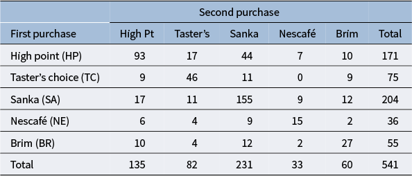
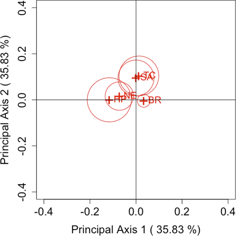

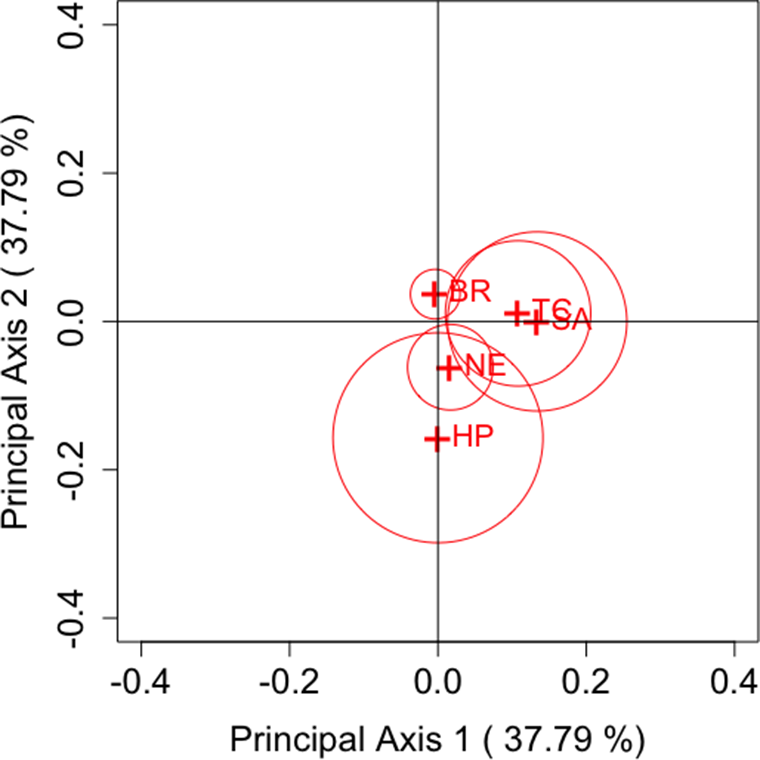

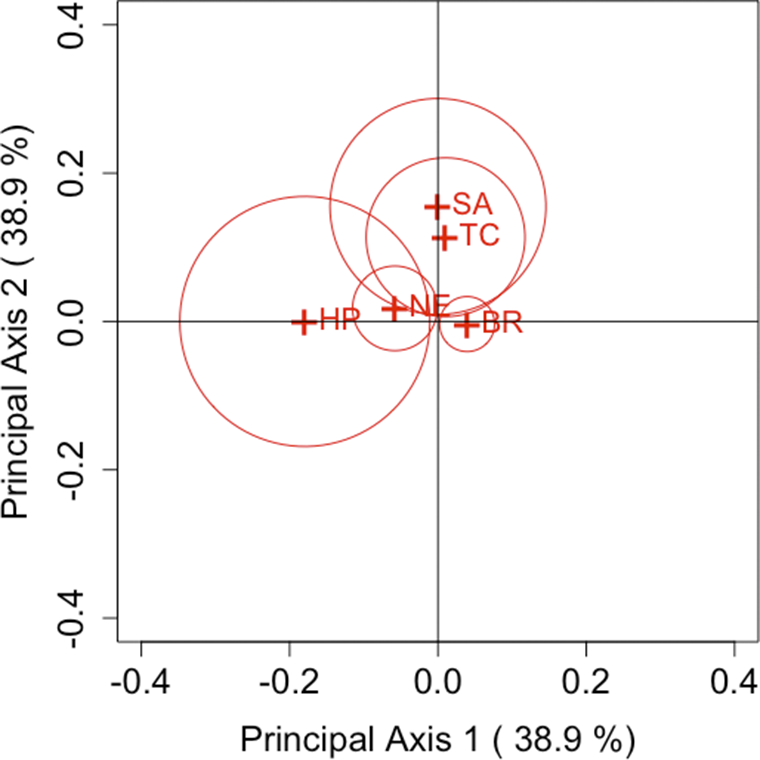

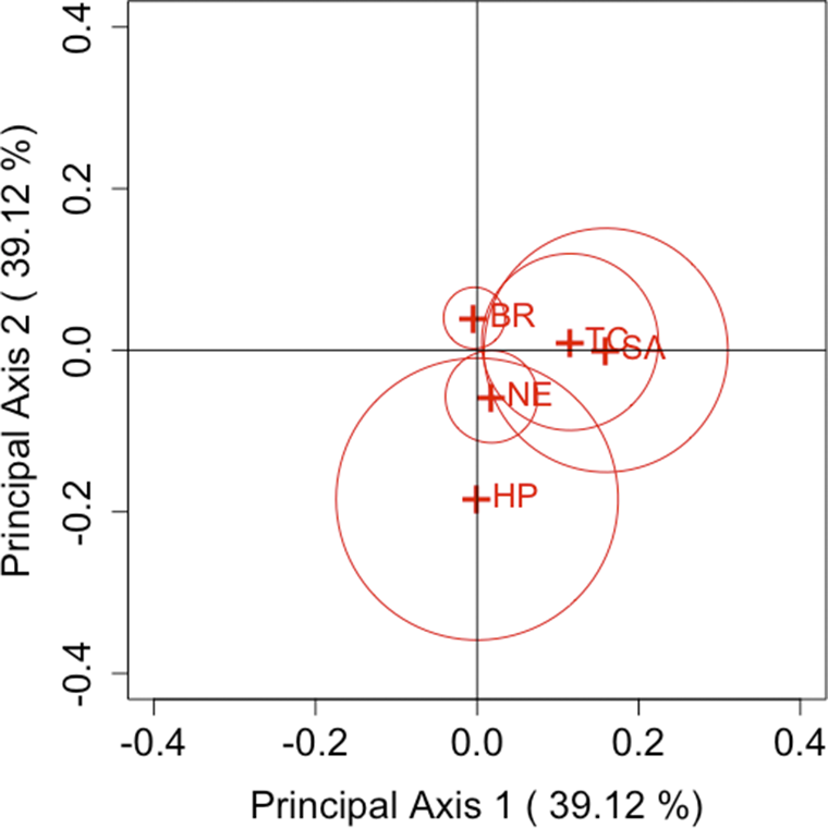

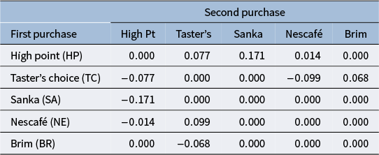


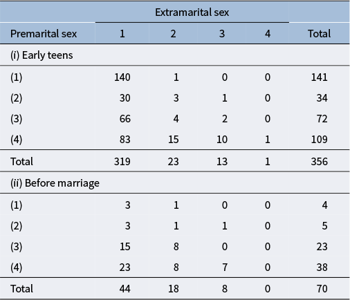
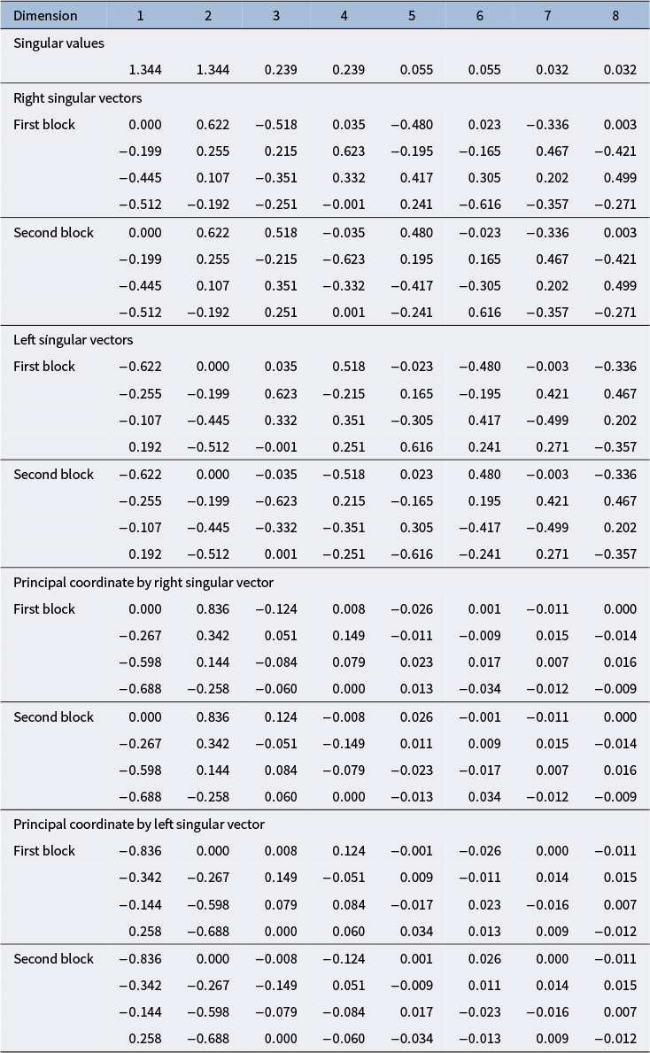

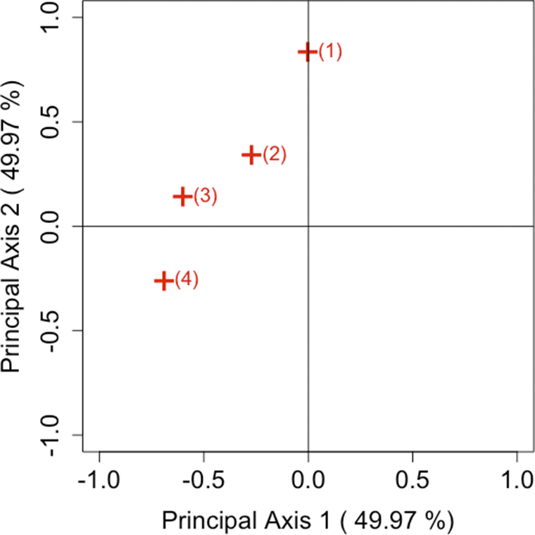

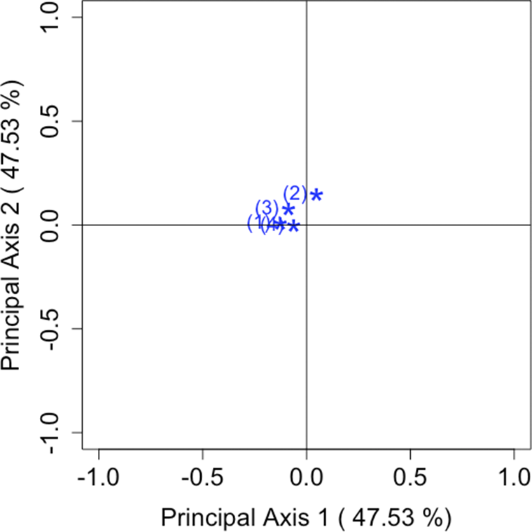

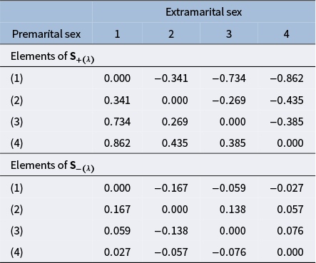


 Open access