


Introduction
Rice is one of the most important and widely consumed cereal staples worldwide and is a significant commodity in the United States (Singh et al. Reference Singh, Zhou, Ganie, Valverde, Avila, Marchesan, Merotto, Zorrilla, Burgos and Norsworthy2017). In 2022, rice was planted in an area of 789.137 thousand hectares, with a total rough rice production of 9 million metric tons (USDA-NASS 2023). However, the global population continues to grow, and so does the demand for rice. To meet the growing demand for rice, it is essential to minimize crop losses (Oerke and Dehne Reference Oerke and Dehne2004). Although various factors affect crop yields, weeds are among the most significant contributors. Weeds compete with crops for nutrients, water, sunlight, and space, leading to reduced crop growth and yield (Oerke Reference Oerke2006). Weeds can also harbor insect pests and diseases that damage or reduce crop yields and interfere with crop management practices such as planting, irrigation, and harvesting (Antralina et al. Reference Antralina, Istina and Simarmata2015; Gibson et al. Reference Gibson, Young and Wood2017; Webster et al. Reference Webster, Bergeron, Blouin, McKnight and Osterholt2018). Among the available weed control methods, herbicide application is the most popular and economically viable option in conventional rice production in the United States (Gianessi Reference Gianessi2013; Smith and Shaw Reference Smith and Shaw1966). However, there are growing concerns about the traditional approach whereby herbicides are broadcast applied throughout the field, especially when weed densities are low. This approach leads to high production costs and potential risks to human and environmental health.
Precision agriculture is transforming production systems through the use of unmanned aerial vehicles, sensors, remote sensing, and digital image processing technologies. These advanced technologies enable growers to obtain site-specific, real-time data on spatial and temporal variability in agricultural fields. Additionally, the combination of drone technology and image analysis techniques has led to significant advancements in site-specific weed management (Hassler and Baysal-Gurel Reference Hassler and Baysal-Gurel2019; Tsouros et al. Reference Tsouros, Bibi and Sarigiannidis2019). Farmers can now accurately identify and target individual weeds in their fields, enabling the precise application of herbicides only where needed (Lati et al. Reference Lati, Rasmussen, Andujar, Dorado, Berge, Wellhausen, Pflanz, Nordmeyer, Schirrmann and Eizenberg2021; Yang et al. Reference Yang, Prasher, Landry and Ramaswamy2003). The site-specific approach is expected to be cost-effective while minimizing potential human health risks and the environmental footprint of herbicide-based weed control (Sapkota et al. Reference Sapkota, Stenger, Ostlie and Flores2023).
Researchers have investigated the effectiveness of site-specific herbicide applications in agriculture. For instance, Hunter et al. (Reference Hunter, Gannon, Richardson, Yelverton and Leon2020) used an unmanned aerial sprayer (UAS) system for weed mapping and spot spraying in sod production fields and found that the UAS-based precision application was up to three times more efficient than ground-based broadcast applications. However, drone-based site-specific applications missed 25% to 30% of targeted weed patches compared to only 2% to 3% in the broadcast method. Using site-specific drone spray in a vineyard, Campos et al. (Reference Campos, Llop, Gallart, García-Ruiz, Gras, Salcedo and Gil2019) reported a 45% reduction in herbicide use compared to a broadcast application, while not compromising weed control efficacy. Other studies have also shown significant reductions in herbicide use with site-specific weed control by up to 90% compared to broadcast applications (Berge et al. Reference Berge, Rene cederkvist, Aastveit and Fykse2008; Genna et al. Reference Genna, Gourlie and Barroso2021; Gerhards and Christensen Reference Gerhards and Christensen2003; Timmermann et al. Reference Timmermann, Gerhards and Kühbauch2003). Moreover, a recent economic analysis conducted by Rajmis et al. (Reference Rajmis, Karpinski, Pohl, Herrmann and Kehlenbeck2022) showed a 26% to 66% reduction in herbicide application costs without affecting crop yield.
Weeds that survive early-season management or emerge later in the crop (i.e., late-season weed escapes) receive little management attention because these weeds do not necessarily lead to significant crop yield loss in the current season, but they do contribute to weed seedbank replenishment and future weed problems (Bagavathiannan and Norsworthy Reference Bagavathiannan and Norsworthy2012; Werner et al. Reference Werner, Sarangi, Nolte, Dotray and Bagavathiannan2020). For example, an uncontrolled escape of hemp sesbania can produce up to 21,500 seeds plant−1 (Lovelace and Oliver Reference Lovelace and Oliver2000). Similarly, yellow nutsedge can produce 20,000 tubers m−2 (Ransom et al. Reference Ransom, Rice and Shock2009), while barnyardgrass can generate 215,000 seeds m−2 (Bagavathiannan et al. Reference Bagavathiannan, Norsworthy, Smith and Burgos2011). A conventional control method for late-season weed escapes involves applying broadcast herbicides across the entire field, even though these escapes may appear at low densities. In this regard, site-specific herbicide applications using remotely piloted aerial application systems (RPAAS) (a more technical term for unmanned aerial sprayers) may provide an effective alternative.
Researchers have used different methods for detecting and mapping weed escapes. Kutugata et al. (Reference Kutugata, Hu, Sapkota and Bagavathiannan2021) utilized UAS-based imagery and vegetation indexes for estimating seed production potential in late-season weed escapes in row crops. However, species identification in more complex species mixes may require more robust remote sensing techniques and tools. Sapkota et al. (Reference Sapkota, Singh, Neely, Rajan and Bagavathiannan2020) employed deep neural networks along with a feature selection method to detect Italian ryegrass [Lolium perenne ssp. multiflorum (Lam.) Husnot] weed in wheat (Triticum aestivum L.) using UAS-based RGB imagery and showed that this approach has the potential for mapping and quantifying ryegrass infestation in wheat. Shahbazi et al. (Reference Shahbazi, Ashworth, Callow, Mian, Beckie, Speidel, Nicholls and Flower2021) used a light detection and ranging sensor (LIDAR) for the differentiation and localization of wild oat (Avena fatua L.) and annual sowthistle (Sonchus oleraceus L.) weeds in wheat based on height differences. Although they show that 90% of weed patches could be easily differentiated from the crop, it is unclear whether such approaches will be effective for weed patches that are of similar height to the crop or shorter. Andújar et al. (Reference Andújar, Rueda-Ayala, Moreno, Rosell-Polo, Escolá, Valero, Gerhards, Fernández-Quintanilla, Dorado and Griepentrog2013) also used a LIDAR sensor to locate the position of weeds, such as barnyardgrass, red dead-nettle (Lamium purpureum L.), and catchweed (Galium aparine L.), that grew shorter than the maize (Zea mays L.) crop canopy and found that the detection accuracy decreased when the scanning distance increased. Moreover, the detection accuracy was also influenced by the size of the object and the target’s orientation toward the LIDAR, suggesting a significant limitation.
López-Granados et al. (Reference López-Granados, Jurado-Expósito, Peña-Barragán and García-Torres2006) used multispectral and hyperspectral imagery for late-season grass weed discrimination and mapping in wheat; their results suggest that mapping grass weed patches was feasible 2 to 3 wk before crop senescence. Koger et al. (Reference Koger, Shaw, Watson and Reddy2003) developed a multispectral imagery–based crop and weed discrimination model for late-season weed detection in soybean [Glycine max (L.) Merr.] that was 78% to 90% accurate. Sivakumar et al. (Reference Sivakumar, Li, Scott, Psota, Jhala, Luck and Shi2020) developed a convolutional neural network (CNN) and faster R-CNN (region-based CNN) model for mid- to late-season weed patch identification in soybean. The results show that the developed model was 92% accurate and that the faster R-CNN had higher performance with lower inference time than the CNN model. However, manually annotating images and training machine learning models are labor intensive and time consuming.
In rice, managing late-season weed escapes with RPAAS-based site-specific herbicide applications can be not only efficient but also convenient because of the challenges with ground herbicide applications due to flooded conditions. Moreover, limited field accessibility also limits other weed management options, such as physical and mechanical methods, making herbicides the most preferable tool. The majority of existing research in this area deals with row crops where species detection can be relatively easier compared to the dense species mixtures expected in rice fields, which are typically planted with narrow row spacing. Furthermore, it is unknown whether such dense species mixtures can influence the efficacy of RPAAS-based herbicide applications for treating weed escapes. These knowledge gaps need to be addressed for developing effective drone-based solutions for targeting late-season weed escapes. The specific objectives of this study were to (1) identify late-season weed patches in rice using different image analysis techniques and (2) compare the efficacy of RPAAS-based precision herbicide application with conventional backpack spray application.
Materials and Methods
Location and Data Collection
The experiments were conducted at the Texas A&M AgriLife Research’s David Wintermann Rice Research and Extension Station, Eagle Lake, TX (30.035°N, 96.604°W), during summer 2021 and 2022 (Figure 1). The location is characterized by a subtropical climate with mild winters and very hot, humid summers.
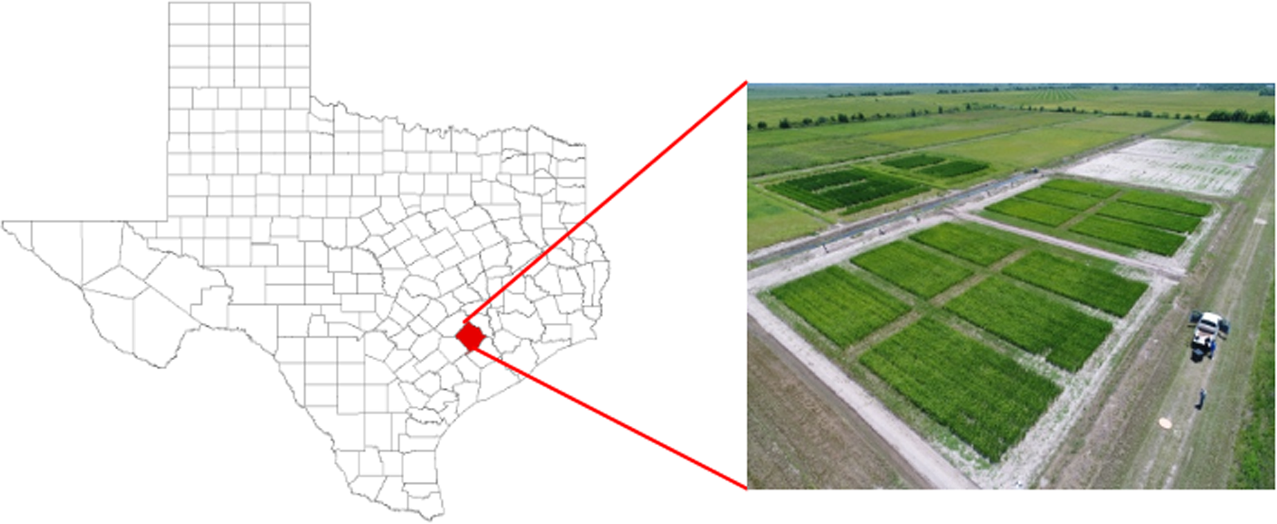
Figure 1. Study area at Texas A&M AgriLife Research’s David Wintermann Rice Research and Extension Station, Eagle Lake, TX.
Experimental Setup and Design
The experiment consisted of four treatments: (1) backpack broadcast application (conventional practice), (2) image analysis–based waypoint extraction and RPAAS-based automatic spot spraying, (3) manual waypoint collection and RPAAS-based automatic spot spraying, and (4) untreated control. The experimental plots were 20 m long and 10 m wide, and each treatment was replicated four times in a randomized complete block design. Evaluations were conducted on naturally occurring weeds in the experimental area. In 2021, the experimental plots were infested with barnyardgrass, Amazon sprangletop, hemp sesbania, and yellow nutsedge, whereas the experimental site in 2022 had infestations of barnyardgrass, Amazon sprangletop, and hemp sesbania only. Rice crop (‘CL153’ at 80 kg ha−1) was grown in a direct-drill-seeded, delayed flooded production system, following the recommended agronomic practices (Way et al. Reference Way, McCauley, Zhou and Wilson2014).
Image Data Acquisition
Aerial images were collected using the RedEdge-M multispectral sensor (MicaSense®, Seattle, WA, USA) mounted on a Matrice 600 Pro drone (DJI®, Shenzhen, China). The flights were carried out at an altitude of 20 m above the ground and a speed of 4 km h−1, 60 d after rice seeding, when the weeds had reached a height similar to or taller than the rice crop. Radiometric calibration was performed using calibration panels, and all the images were collected during solar noon using a grid pattern with 80% front and side overlap. To ensure accurate mapping, six ground control points (GCPs) were deployed across the field, and a handheld real-time kinematic (RTK) GNSS unit (Reach RS2+, Emlid®, Budapest, Hungary) was used to collect the latitude and longitude of each GCP. The Pix4Dmapper software (Lausanne, Switzerland) was used with the “Ag Multispectral” template to produce an orthomosaic image. The orthomosaic image was georeferenced to the World Geodetic System 1984 coordinate system during the mosaicking process, and the resulting image had a spatial resolution of 1.3 mm pixel−1, which was suitable for this study.
Manual Waypoints
In the experimental plots, the center of each weed patch was manually marked using the handheld RTK-GNSS unit. This involved walking into the rice field, locating the waypoints, and physically marking them. The waypoints were then converted into an Esri shapefile and uploaded onto an RPAAS spray drone for automatic navigation.
Image Analysis–Based Waypoints
After the orthomosaic was generated, a Python-based rice–weed model was developed to extract global waypoints of weed escapes from the aerial imagery. The model utilized the canopy height model (CHM) and the spectral response of rice and weeds. The CHM was calculated using a digital surface model and a digital terrain model, which helped detect weed patches that were taller than the rice canopy. Similarly, to distinguish weeds from rice based on spectral reflectance, red, green, blue, red-edge, and near-infrared bands and their combinations were tested (Figure 2). It was found that yellow nutsedge and sprangletop were visible in the blue and red bands. In general, the red band was more effective at distinguishing rice from weeds than was the blue band. A threshold value was set for the CHM and red band through a trial-and-error approach. Any value below the threshold was eliminated, including nontarget areas such as soil background and rice canopy. The threshold value for CHM was set at 0.08 m, while for the red band, it was set at 28 digital number (DN). Additionally, morphological operations (dilation) were performed to enhance the area of the detected object in the image. After weed patch delineation, each patch was converted into a polygon, and a center point was determined for each polygon using the moment determination method (https://docs.opencv.org/3.4/d0/d49/tutorial_moments.html). Any polygon with an area of less than 0.05 m2 was eliminated to reduce noise and remove unwanted pixel areas from the data. To recognize potential duplicate points, a Python function was used that employed the Euclidean distance metric and set the Euclidean threshold value based on the sprayer ground coverage area (0.60 m). The CHM- and red band–based weed coordinates were then combined into a single data frame using the union function in GeoPython (https://geo-python-site.readthedocs.io/en/latest/). Finally, the geospatial packages rasterio and geopandas were used to transform polygon center points into global coordinates (WGS84) and subsequently convert global coordinates into an Esri shapefile to direct automatic navigation of the RPAAS to the specific weed patches (Figure 3).
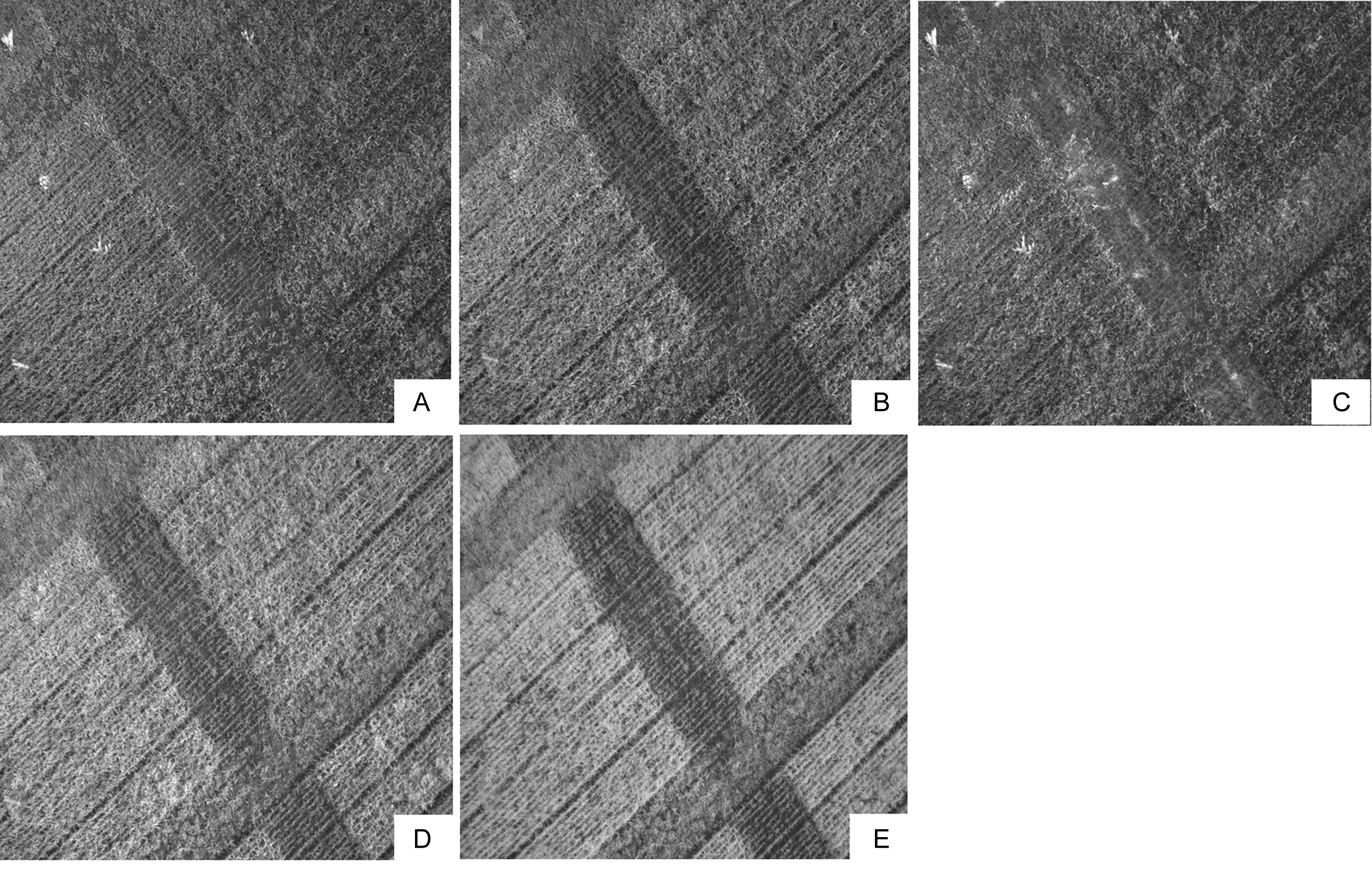
Figure 2. Example of distinctive reflectance for rice and weeds in multispectral (MicaSense® RedEdge-M) imagery captured 60 d after rice planting: blue band (A), green band (B), red band (C), red-edge band (D), and near-infrared band (E). The sensors were mounted on a DJI® Matrice 600 Pro drone flying at an altitude of 20 m.
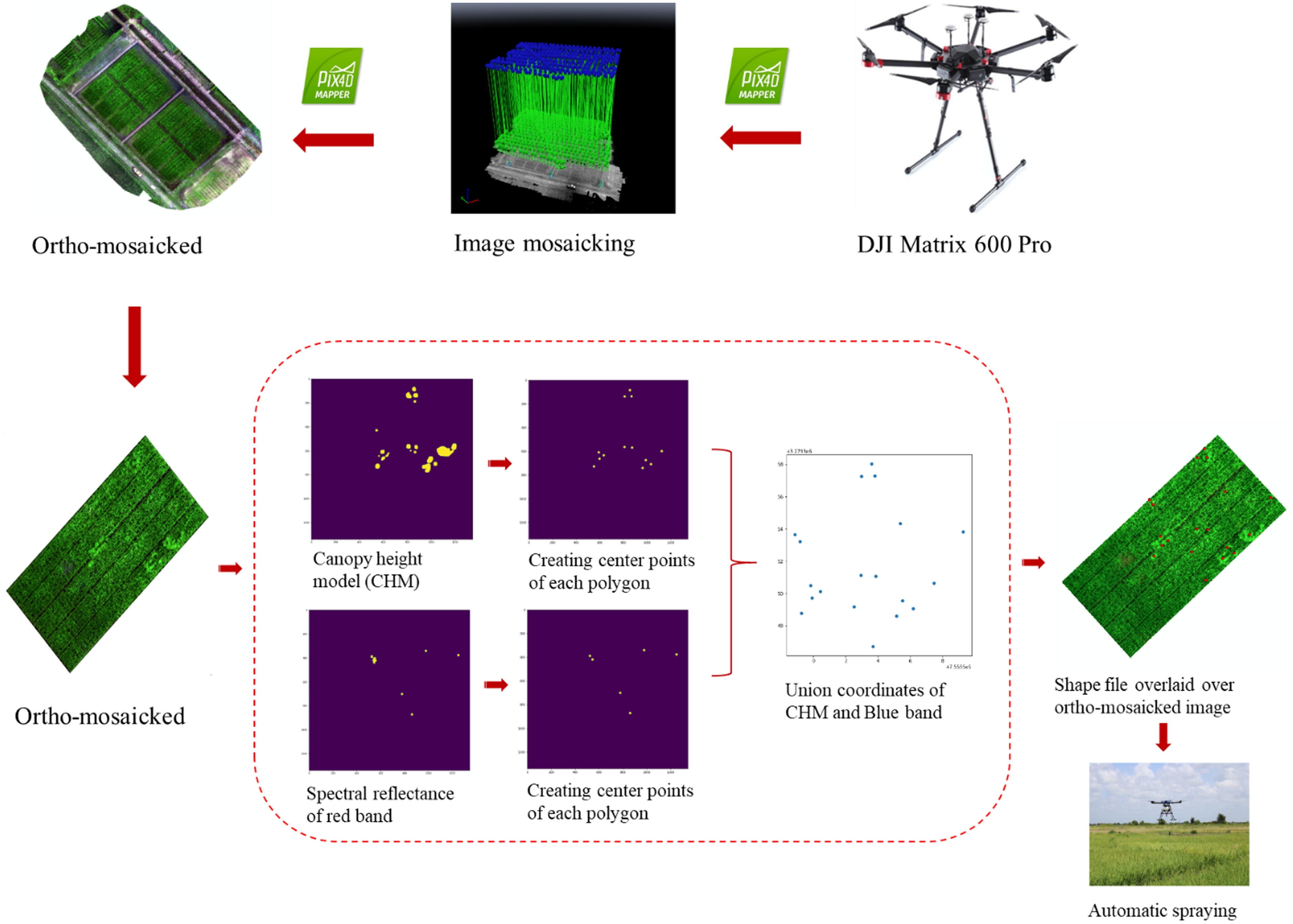
Figure 3. Schematic describing the workflow from aerial image collection to analysis, production of shape files, and site-specific spraying.
Model-Based Weed Localization Accuracy Assessment
The localization of weed patches comprises two key aspects: weed detection accuracy and positional accuracy. Weed detection accuracy represents the proportion of weed patches correctly identified by the model in comparison to the actual numbers in the field. On the other hand, positional accuracy reflects the deviation of the detected center point of the weed patch from the manually marked center point, measured in centimeters. To measure both detection and positional accuracy, all the weed patches in the experimental plots were counted manually, and their center points were marked using the Emlid® GNSS unit prior to the UAS flight. Afterward, a Python-based model was used to extract the center coordinates of the weed patches from the orthomosaicked image. The model-based coordinates were then verified for false positives and negatives as well as for positional accuracies based on the manually marked center points.
Sprayer Specifications
Backpack Sprayer
The backpack sprayer was CO2 pressurized and equipped with three TT11002 (TeeJet® Technologies, Glendale Heights, IL, USA) nozzles. The backpack sprayer was calibrated to deliver a spray volume of 140 L ha−1 at an application speed of 1.4 m s−1 with a pressure of 206 kPa.
RPAAS Sprayer
A Precision Vision 35X spray drone (Leading Edge® Aerial Technologies, Fletcher, NC, USA) was used for site-specific spraying (Figure 4). The RPAAS was equipped with a 16-L tank and a single TJ QGA-3007 full-cone nozzle mounted directly under the drone. The drone sprayer was calibrated to deliver 30 ml s−1 at 206 kPa pressure. Flights were made at 2.5 m above ground level at a ground speed of 5.4 m s−1 between points. Upon reaching the specified location, the RPAAS stabilized both its horizontal and vertical positions within 5 s before delivering a 2-s spray. An RTK base station was set up near the experimental field to ensure precise navigation of the RPAAS. For monitoring real-time meteorological data (temperature, humidity, wind speed, and wind direction), a wireless weather station (Vantage Pro2, Davis Instruments, Hayward, CA, USA) was deployed in the field.
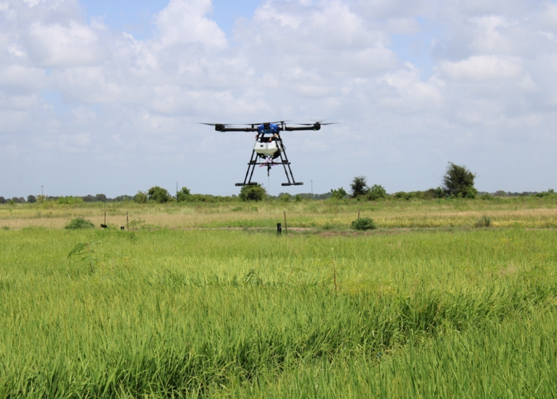
Figure 4. Remotely piloted aerial application system (Leading Edge® Precision Vision 35X; RPAAS) used in the study for targeting individual weed escapes/patches.
Herbicide Applications
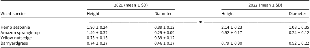
A selective postemergence rice herbicide, florpyrauxifen-benzyl (Loyant®, Corteva Agriscience, Indianapolis, IN, USA), was applied at a rate of 32 g ai ha−1 in both study years. This herbicide provides a broad-spectrum postemergence activity on the range of weed species included in the study. To determine the droplet deposition patterns, Rhodamine red dye (Liquid Red, Cole-Parmer, Vernon Hills, IL, USA) was added to the spray solution at a rate of 0.5% (v/v) for both backpack and RPAAS applications. To capture the spray droplets, Kromekote cards (10 × 5 cm) were placed on the tops of wooden poles (1.5 × 0.05 × 0.02 m) (Figure 5). These poles were deployed randomly around the weed patches before spraying. After the cards were dry, they were placed in an airtight polyethylene zipper bag, and the droplet deposition patterns were analyzed in the laboratory using DropletScan™ software (Zhu et al. Reference Zhu, Salyani and Fox2011). Droplet parameters, such as droplet size, density (droplets cm−2), droplet uniformity (i.e., coefficient of variation), and percent area coverage, were measured. In addition, canopy height and diameter of each weed patch were measured using a ruler before the spray applications (Table 1).
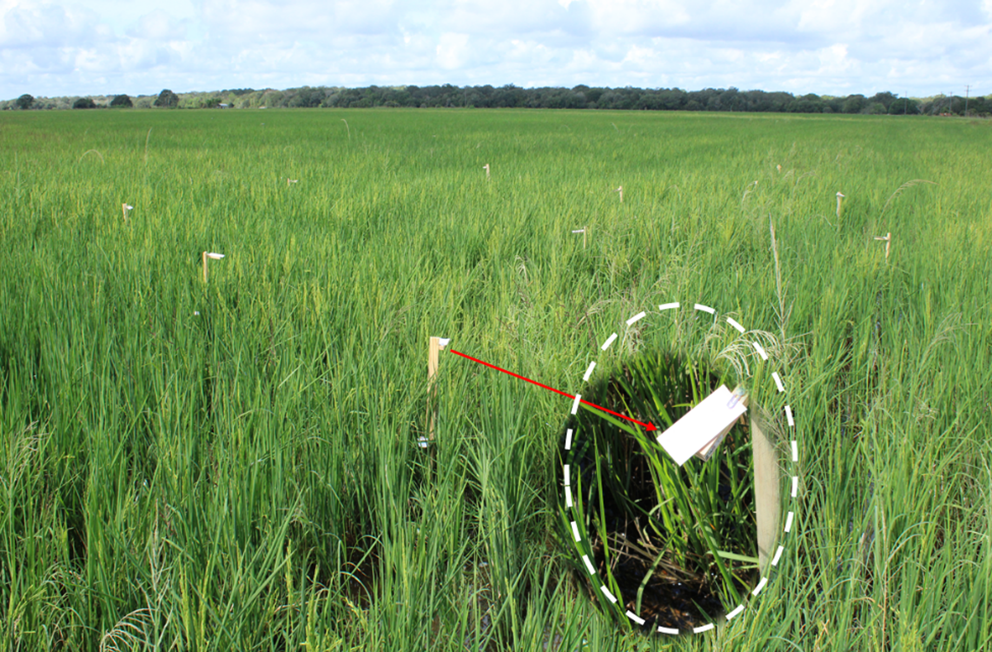
Figure 5. Placement of Kromekote cards on wooden poles in the experimental field for assessing spray droplet distribution. The inset is a close-up of the Kromekote card setup.
Table 1. Plant height and canopy diameter of the weed species evaluated in this study across the two study years.
Visual weed control was evaluated at 28 d after herbicide treatment (DAT) for each weed patch on a scale of 0 (no control) to 100 (complete plant death) to measure herbicide efficacy. Following that, the aboveground weed biomass was harvested, placed in separate brown bags, dried at 60 C for 72 h, and weighed to determine plant biomass reduction (Equation 1):
 $${\rm Biomass\;reduction} =$$
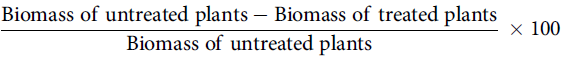 $${{{\rm{Biomass\;of\;untreated\;plants} - {\rm{Biomass\;of\;treated\;plants}}}}\over{{{\rm{Biomass\;of\;untreated\;plants}}}}}\; \times 100$$
The samples were then threshed by hand, and the seeds were cleaned and weighed. At 120 d after rice planting, a 0.8 × 18 m swath of rice was harvested using a self-propelled small plot combine (Mitsubishi plot combine), and rice grain yield was determined at 12% seed moisture content in both years.
Statistical Analysis
Statistical analyses were carried out using R software (version 4.3.2; R Core Team 2024) to estimate the positional error of image-based geocoordinates and compare treatment differences for weed control, plant dry weight, droplet distribution, spray coverage, and grain yield. The ANOVA package aov() in R (linear model) was used to conduct one-way ANOVAs. Treatment was considered as the fixed effect, whereas replication and year were considered as random effects. Treatment mean separations were performed using Tukey’s HSD method at α = 0.05. Prior to conducting ANOVA, the normality of the residuals was checked using the Shapiro–Wilk test; no transformations were necessary. The effectiveness of the sprayers was evaluated by analyzing the volume median diameter (VMD), the uniformity of droplet distribution based on the coefficient of variation (CV) value, and the percentage of spray coverage. Weed biomass data were pooled across the two years; biomass data were not available for yellow nutsedge because the herbicide-treated plants completely degraded in standing water by 28 DAT. A log10 transformation was applied to the weed biomass data prior to conducting ANOVA.
Results and Discussion
Late-Season Escaped Weed Patch Delineation in Rice
The weed detection model was developed using an integrated approach that combined the CHM and red wavelength spectral signatures to differentiate between rice plants and weed escapes. Among the targeted species, hemp sesbania exhibited the highest detection accuracy, with Amazon sprangletop, yellow nutsedge, and barnyardgrass following in descending order.
Hemp sesbania, known for its tall growth, open canopy, and high biomass, was distinctly detectable by the CHM, leading to the highest detection accuracy across both years. In 2021, the detection accuracy was 91%, with an average height and diameter of 1.90 m and 0.89 m, respectively. The detection accuracy improved to 93% in 2022, possibly due to an increase in plant size, with the average height and diameter reaching 2.14 m and 1.08 m, respectively. However, if the hemp plant’s height was equal to or less than the rice canopy’s, it remained undetectable by both CHM and spectral signature methods. Shahbazi et al. (Reference Shahbazi, Ashworth, Callow, Mian, Beckie, Speidel, Nicholls and Flower2021) reported similar findings that the LIDAR sensor detected wild oat and annual sowthistle in wheat crops with 100% accuracy when the weeds were taller than the wheat canopy.
The detection of Amazon sprangletop was facilitated by its long and distinct seed heads, which stood out from the rice crop and other weed species. These seed heads exhibited a unique spectral signature in the red band (668 nm) (Figure 2 C). In 2021, the detection accuracy was 87%. In 2022, however, the detection accuracy dropped to 85%, possibly due to a reduction in the size of the weed patch (0.92 m tall and 0.24 m wide, compared to 1.49 m and 0.29 m, respectively, in 2021), which may have reduced the detection accuracy. This result was supported by McCormick (Reference McCormick1999), whereby the distinctive cylindrical crown shape of paperbark-tree [Melaleuca quinquenervia (Cav.) S.F. Blake] enabled the identification of this invasive tree in aerial imagery. A study was conducted by El Imanni et al. (Reference El Imanni, El Harti, Bachaoui, Mouncif, Eddassouqui, Hasnai and Zinelabidine2023), using a combination of spectral bands and the CHM, to classify citrus and weeds. The study found that incorporating CHM increased the classification accuracy by 13.4% when compared to relying solely on spectral signatures. Yellow nutsedge presented challenges with detection due to its size, which caused it to blend into the rice canopy. In 2021, the detection accuracy for yellow nutsedge was 74%, with average height and canopy diameter of 0.73 m and 0.37 m, respectively. Detection relied solely on spectral signatures because there was no significant height differentiation between the weed and the rice crop. However, the yellow flower head of the nutsedge displayed a distinct spectral signature in the red band when the weed patch was large enough (approximately 125 cm2 in area) (Figure 2). This finding corroborates with Che’Ya et al. (Reference Che’Ya, Dunwoody and Gupta2021), who detected yellow nutsedge in the red-edge region (720 nm) in sorghum [Sorghum bicolor (L.) Moench]. Yellow nutsedge was not found in the experimental plots in 2022.
Barnyardgrass posed the most significant detection challenge due to its high degree of mimicry with the rice crop. In 2021, it had the lowest detection accuracy at 63%, with an average height of 0.74 m and a canopy diameter of 0.46 m, similar to the rice crop. Detection was much easier when the weed plant was taller than the rice canopy. However, the high variability in barnyardgrass heights across the field led to lower overall detection accuracy (Table 2). In 2022, though barnyardgrass was taller and wider (0.79 m and 0.22 m, respectively), the detection accuracy further declined to 59%. This may have been due to the overall variability in plant height and canopy diameter observed, coupled with the phenotypic similarity to rice, which may have made discrimination very difficult (Yang and Chen Reference Yang and Chen2004; Zhang et al. Reference Zhang, Gao, Cen, Lu, Yu, He and Pieters2019).
Table 2. Weed detection accuracy assessment and center point estimation of the image-based geocoordinate method across the two study years. a,b
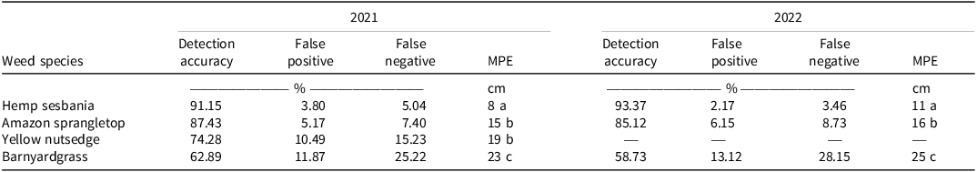
a Means followed by different letters within a column are significantly different according to Tukey’s HSD (α = 0.05).
b Abbreviation: MPE, mean positional error.
Positional Accuracy of Detected Weed Patch
Image-Based Weed Localization Accuracy
The positional accuracy, or error, reflects the difference in the estimation of the center point of a weed patch between the model-based predicted center point and the manually marked center point. The positional error was due to the combined effects of the individual weed species’ geometry, the accuracy of georeferenced images, and the accuracy of the ground control points (GCP) (Elkhrachy Reference Elkhrachy2021; Sánchez et al. Reference Sánchez, Cuartero, Barrena and Plaza2020; Figure 6).
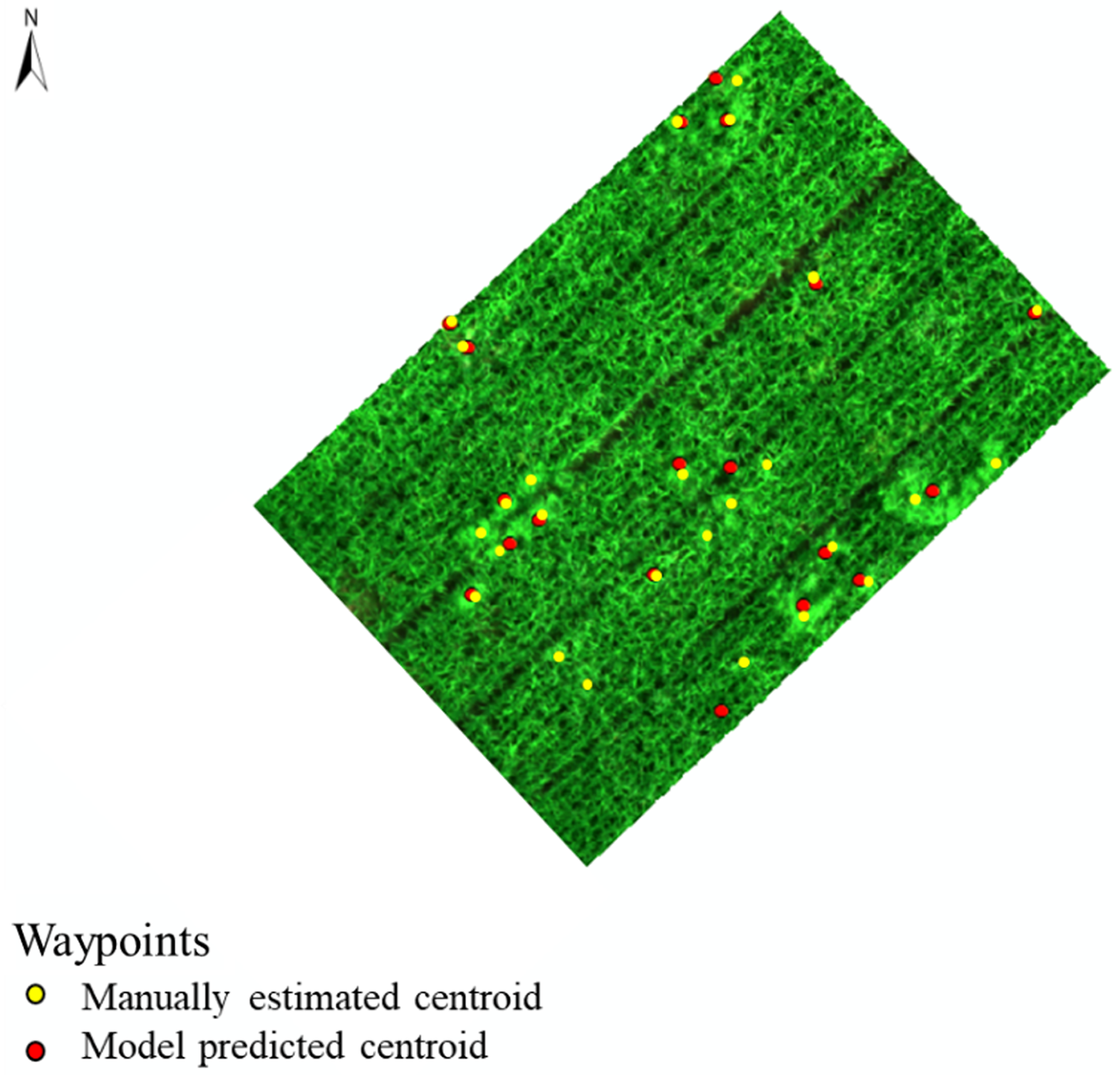
Figure 6. An orthomosaicked image of the experimental area showing the locations of weed escapes, determined either using a handheld RTK-GPS device (yellow circles) or based on an image analysis–based predictive model (red circles).
The degree of positional accuracy varied among the weed species and, to some extent, between the two flights (i.e., study years). For hemp sesbania, the average error in estimating the center point was 8 cm in 2021, the smallest among the weed species. This was due to its large size, which made its entire geometry visible in the CHM, making it easier to locate the center point of the weed patch compared to the other weed species targeted. In 2022, the error for hemp sesbania increased slightly to 11 cm, with this species again showing the lowest detection error among the weeds studied. The average error for Amazon sprangletop ranged 15 to 16 cm for the two flights; this error was larger than the error for hemp sesbania, possibly due to the more open growth habit of this species, leading to inaccuracies in locating the exact center point of the patch (Ronay et al. Reference Ronay, Kizel and Lati2022).
Yellow nutsedge had average error of 19 cm in 2021, which was greater than those of hemp sesbania and Amazon sprangletop; in 2022, yellow nutsedge was not found in the experimental field. This high error was likely due to its canopy geometry, which caused it to blend into the rice canopy, making it difficult to locate the exact center point of the weed patch. Barnyardgrass had the highest average error among the weed species studied here in both years. In 2021, the error was 23 cm, likely due to its diverse geometry and high mimicry with the rice crop. In 2022, the error increased to 25 cm, despite an increase in height and diameter of the weed canopy compared to the previous year.
The findings suggest that the identification of the center point of weed patches is directly influenced by the weed’s detectable geometry in the imagery. When a weed patch is distinct in the image, the model accurately locates its center point. However, if the patch is less visible, the estimated center point may be offset from the true center. Additionally, orthomosaic image stitching errors, influenced by UAS GPS inaccuracies and environmental factors, are measured using root mean square error (RMSE). This error directly affects the position of targeted weeds for precision spraying, particularly on small patches. The RMSE of the orthomosaic image was 9 cm in 2021 and 12 cm in 2022. This RMSE in the mosaicked image directly contributes to errors in the image-based waypoints. These results align with those of Benassi et al. (Reference Benassi, Dall’Asta, Diotri, Forlani, Morra di Cella, Roncella and Santise2017), who reported an RMSE of approximately 2 to 3 cm using an eBEE RTK; though these error values are low, they may still lead to inaccurate spray applications on small weed patches.
Manual Weed Localization Accuracy
The accuracy of manually located waypoints and GCP depends on the RTK-GNSS unit accuracy and how accurately the center of each weed patch and GCPs were marked. The handheld Reach RS2+ RTK-GNSS unit had average longitude and latitude error of 1.9 cm and 1.5 cm, respectively. However, this error may vary with various environmental factors, such as ionospheric activity, tropospheric activity, and signal obstructions (Baybura et al. Reference Baybura, Tiryakioğlu, Uğur, Solak and Şafak2019).
Weed Control Efficacy
Weed Injury
The backpack method consistently demonstrated the highest weed control efficacy across all treatments, regardless of weed species or year, followed by RPAAS with manually collected geocoordinates. In contrast, RPAAS with image-based geocoordinates showed the lowest efficacy. The overall effectiveness of all three treatments was slightly lower in 2022 than in 2021, possibly due to factors like weed patch geometry, RPAAS navigational accuracy, wind speed, and model-based detection accuracy (P < 0.0001) (Figure 7).
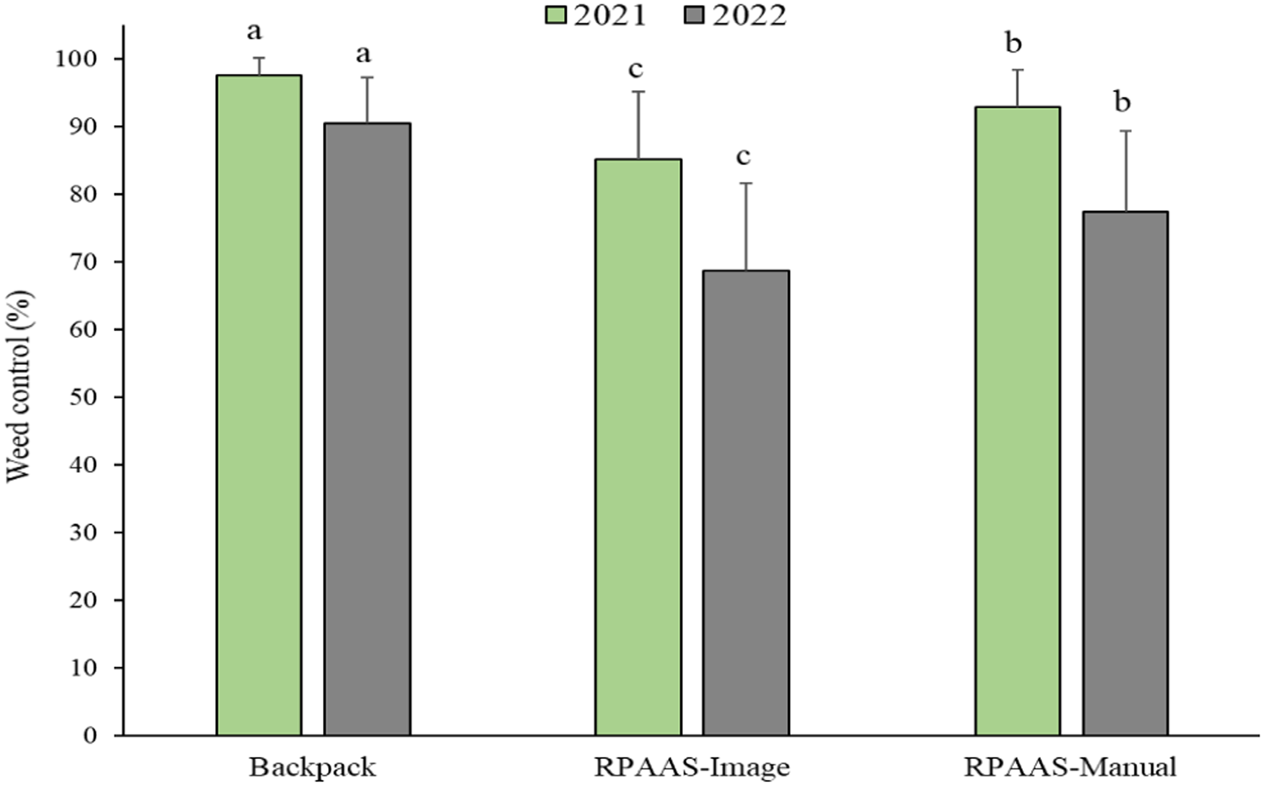
Figure 7. Comparison of overall weed control efficacy (%) between a backpack sprayer and an RPAAS (with manual GPS coordinate or image-based method) for the entire weed spectrum present in the experimental field for the two study years. The bars topped with different letters indicate significant differences based on Tukey’s HSD (α = 0.05). The whiskers on the bars represent standard errors of the mean.
Hemp sesbania control showed a significant difference between the three treatments in the 2021 experiment (P < 0.0001). The backpack spray application had the highest weed control efficacy (95%), followed by the RPAAS with manually collected geocoordinates (87%) and the RPAAS with image-based geocoordinates (72%) (Figure 8). The reduced efficacy of the image-based method was likely due to the weed patch detection and localization errors. Additionally, the tall stature of hemp sesbania made it particularly vulnerable to RPAAS downwash (Figure 9 A), which caused the plants to lodge away from the center of the target location, making it difficult to treat the entire patch, in turn resulting in reduced coverage areas (Zhang et al. Reference Zhang, Wen, Chen, Liu, Xu, Chen and Lan2023). Canopy displacement was not an issue with backpack applications. It was further observed that RPAAS sometimes deviated from the target during spraying, likely due to navigational errors (Hodgson and Bresnahan, Reference Hodgson and Bresnahan2004) (Figure 9 B). Navigational error could not be measured during RPAAS flight and was instead based on visible observations by the RPAAS flight crew members. In 2022, the overall control efficacy of hemp sesbania was lower than in 2021 (Figure 8). The backpack method again achieved the highest control efficacy (82%), followed by RPAAS manual (74%) and RPAAS image-based (63%) methods (P < 0.001). The reduced efficacy in 2022 was likely due to one or more of the following factors: variation in the size of hemp sesbania patches, higher RPAAS navigation errors, and difficulties in accurately locating the weed patch centers (Table 2), ultimately resulting in poor herbicide coverage.
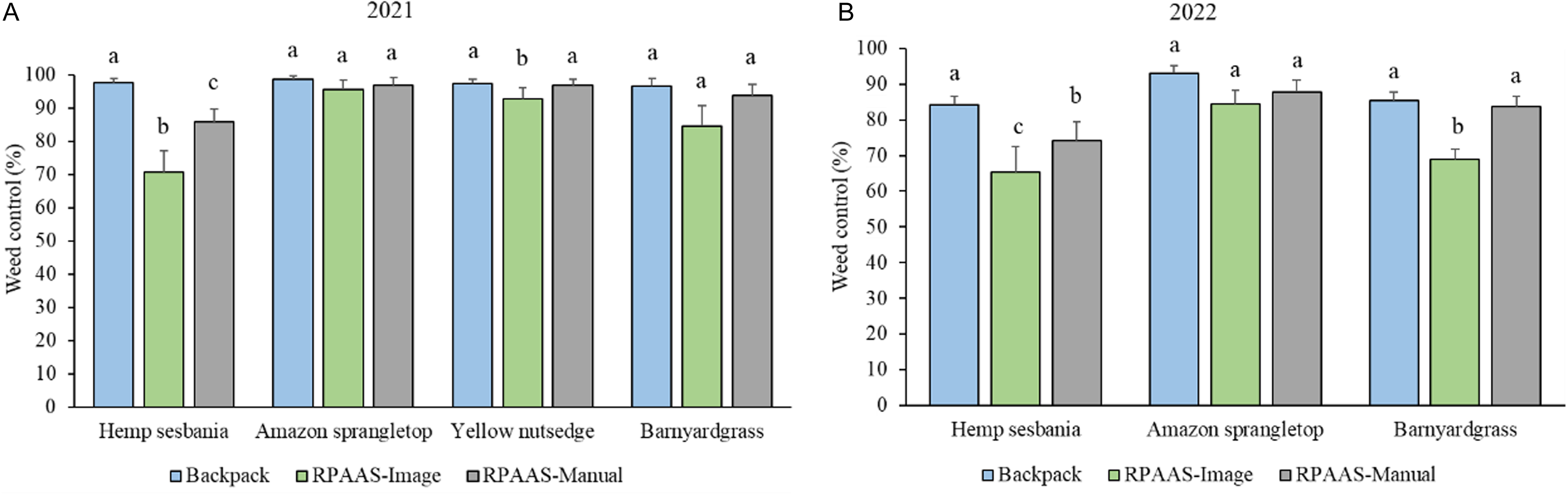
Figure 8. Comparison of weed control efficacy (%) between a backpack sprayer and a drone sprayer (with manual GPS coordinate method or image-based GPS coordinate method). The bars topped with different letters indicate significant differences based on Tukey’s HSD (α = 0.05). The whiskers on the bars represent standard errors of the mean.
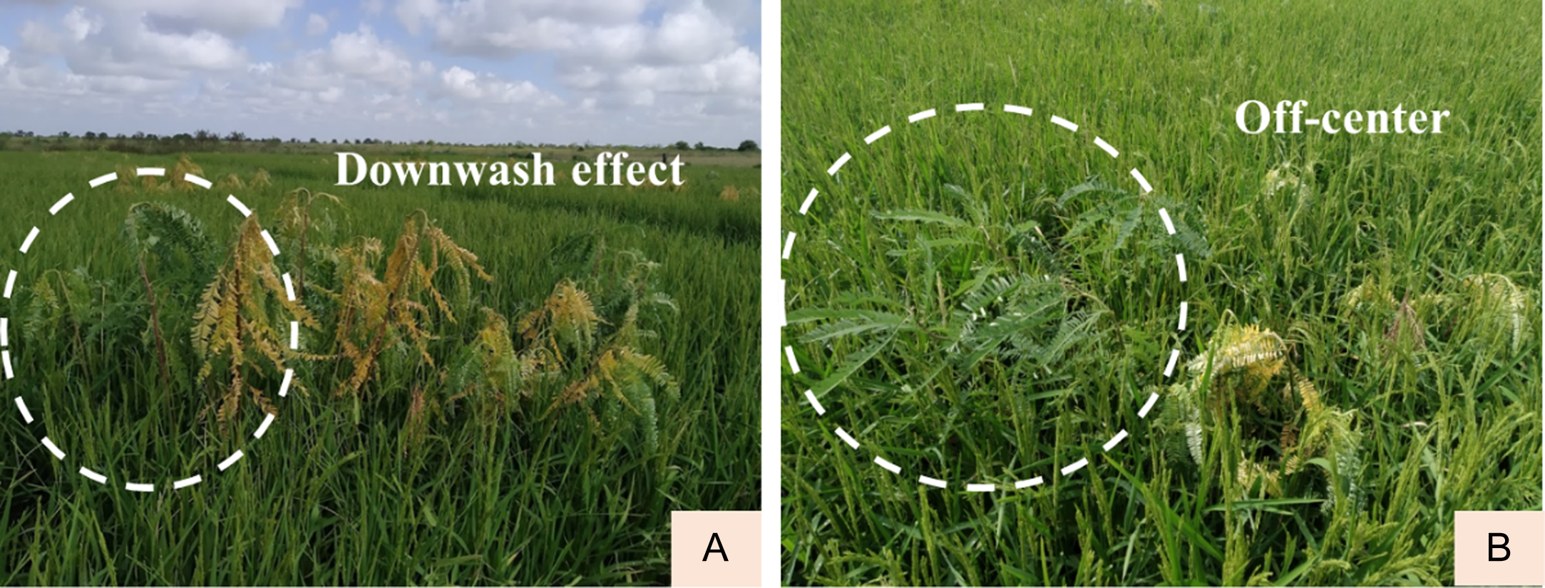
Figure 9. Examples of spray coverage errors observed in this study: poor coverage on hemp sesbania due to lodging (downwash effect of rotors) (A) and position error associated with image-based coordinates (B).
For Amazon sprangletop, the control efficacy in 2021 showed a trend consistent with that of hemp sesbania. The backpack method achieved the highest efficacy, ranging from 92% to 97%, followed by the RPAAS manual method (87% to 96%); the RPAAS image-based method had the lowest efficacy, ranging from 72% to 87%. Owing to its open growth habit and shorter stature than hemp sesbania, Amazon sprangletop was less impacted by RPAAS downwash, resulting in better herbicide coverage and higher control efficacy. In 2022, a similar trend was observed regarding Amazon sprangletop control. The backpack method achieved the highest control efficacy (94%), followed by RPAAS manual (89%) and RPAAS image (87%). No significant difference was observed between the treatments in 2022 (P = 0.12). For yellow nutsedge, the backpack (95%) and RPAAS manual (93%) methods showed comparable weed control efficacies in 2021, both outperforming the RPAAS image-based method (87%) (P = 0.0086). However, in 2022, yellow nutsedge was not found in the experimental plots. Nevertheless, the data from year 1 still offer valuable insights into yellow nutsedge control using RPAAS-based herbicide applications.
In the case of barnyardgrass, weed control efficacy in 2021 varied as follows: backpack (96%) = RPAAS manual method (92%) > RPAAS image-based method (82%) (Figure 8). The lower efficacy of the image-based geocoordinate method was due to errors in center point estimation (Table 2), which led to poor coverage of individual patches. In 2022, the RPAAS image-based method exhibited significantly lower efficacy than the RPAAS manual method. The backpack (86%) and RPAAS manual (83%) methods showed comparable weed control efficacies, both surpassing the RPAAS image-based method (68%) (P = 0.0046).
Effect of Weather on RPAAS Weed Control Efficacy
The spot spraying method is vulnerable to wind speed and direction; a sudden gust of wind can divert the spray away from the targeted weed patch. Weather data were continuously recorded in real time during herbicide application in both years. The mean air temperature ranged from 28 C to 30 C in 2021, whereas in 2022, it was higher, ranging from 35 C to 38 C. Humidity varied between 55% and 57% in 2021, whereas in 2022, it ranged from 55% to 62%. These parameters were optimal for herbicide application and should not have affected weed control efficacy (Brainard et al. Reference Brainard, Curran, Bellinder, Ngouajio, VanGessel, Haar, Lanini and Masiunas2013; Varanasi et al. Reference Varanasi, Prasad and Jugulam2016). Wind speeds and directions were highly variable in both years (Figure 10). The wind speeds ranged from 2 to 16.2 km h−1 in 2021, which was generally higher than the wind speeds recorded in 2022 (1.5 to 8.8 km h−1).
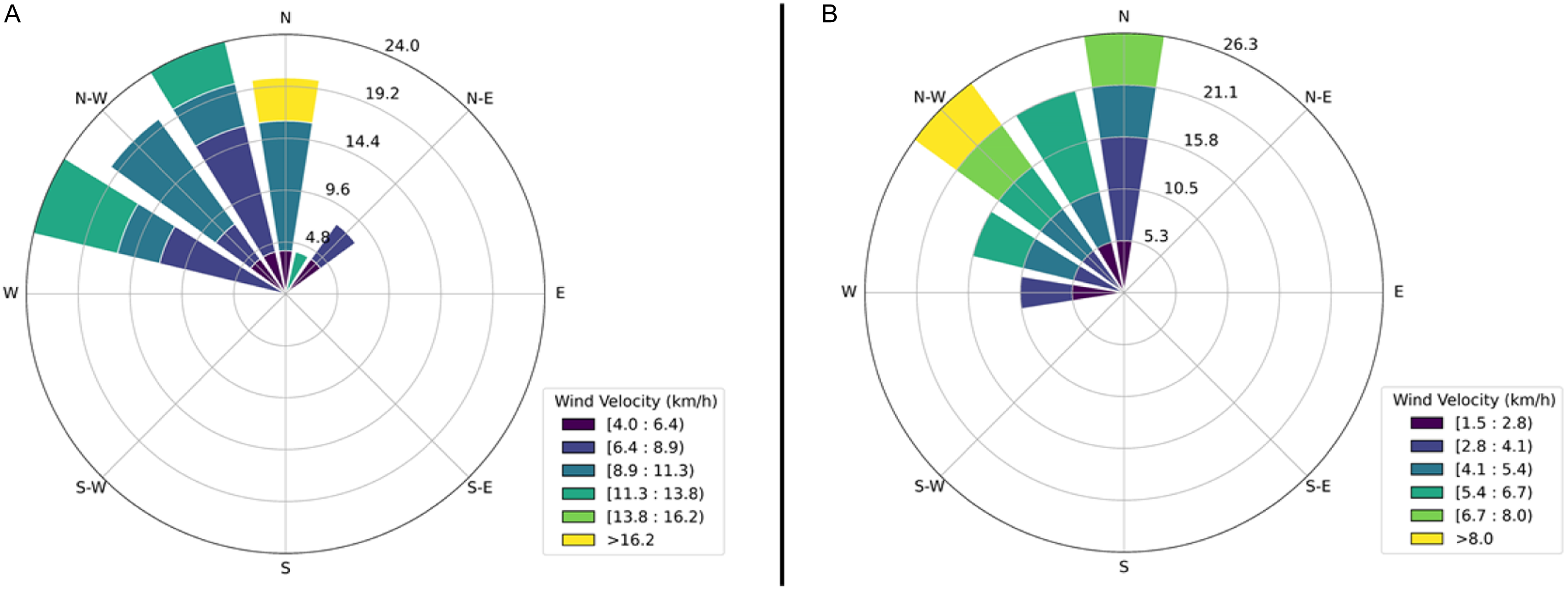
Figure 10. Wind velocity (km h−1) and direction during herbicide applications in 2021 (A) and 2022 (B).
To minimize the wind effect, the RTK base station was adjusted along the wind direction from its initial position using the trial-and-error method. The RTK base station was shifted 30 cm from its original position to compensate for wind speed and direction. A similar approach was used by Guo et al. (Reference Guo, Yao, Xu, Ma, Sun, Chen and Lan2022) in pear (Pyrus ussuriensis Maxim.) orchards using spot spray; they recommended that the drone sprayer move in the upward wind direction if the wind speed is higher than 2 m s−1, to achieve higher droplet deposition and better distribution uniformity. In 2022, the base station was kept in its original position because the wind speed remained fairly within the recommended range for spraying. However, occasional gusts caused the spray to move off-target, reducing weed patch coverage (Figure 9 B) and leading to poor weed control efficacy, as observed previously by Martin et al. (Reference Martin, Woldt and Latheef2019).
It is important to note that shifting the RTK base station may not achieve 100% coverage, and changing the base station in real time during herbicide application to compensate for gusty winds may be challenging. Although the spot spraying method shows promise, its efficacy is significantly influenced by environmental factors like wind speed and direction, requiring careful consideration and adjustment of the RTK base station during application.
Reduction in Weed Biomass
All herbicide treatments, regardless of application method, reduced the biomass of hemp sesbania (Figure 11 A), Amazon sprangletop (Figure 11 B), and barnyardgrass (Figure 11 C) compared to the untreated plants. The backpack application method consistently resulted in the highest biomass reduction across all weed species, with reductions of 57% for hemp sesbania, 54% for Amazon sprangletop, and 53% for barnyardgrass compared to untreated plants. The RPAAS method with manual geocoordinates followed, achieving biomass reductions of 52% for hemp sesbania, 47% for Amazon sprangletop, and 50% for barnyardgrass. The RPAAS method using image-based geocoordinates showed the lowest efficacy, with reductions of 47% for hemp sesbania, 45% for Amazon sprangletop, and 48% for barnyardgrass. Overall, the backpack method provided the most effective weed control, likely due to better herbicide coverage, with the RPAAS methods (manual and image-based geocoordinates) showing lower levels of biomass reduction. Our findings support Hiremath et al. (Reference Hiremath, Khatri and Jagtap2024), who reported higher weed biomass reduction under the knapsack method than with a drone sprayer in soybean.
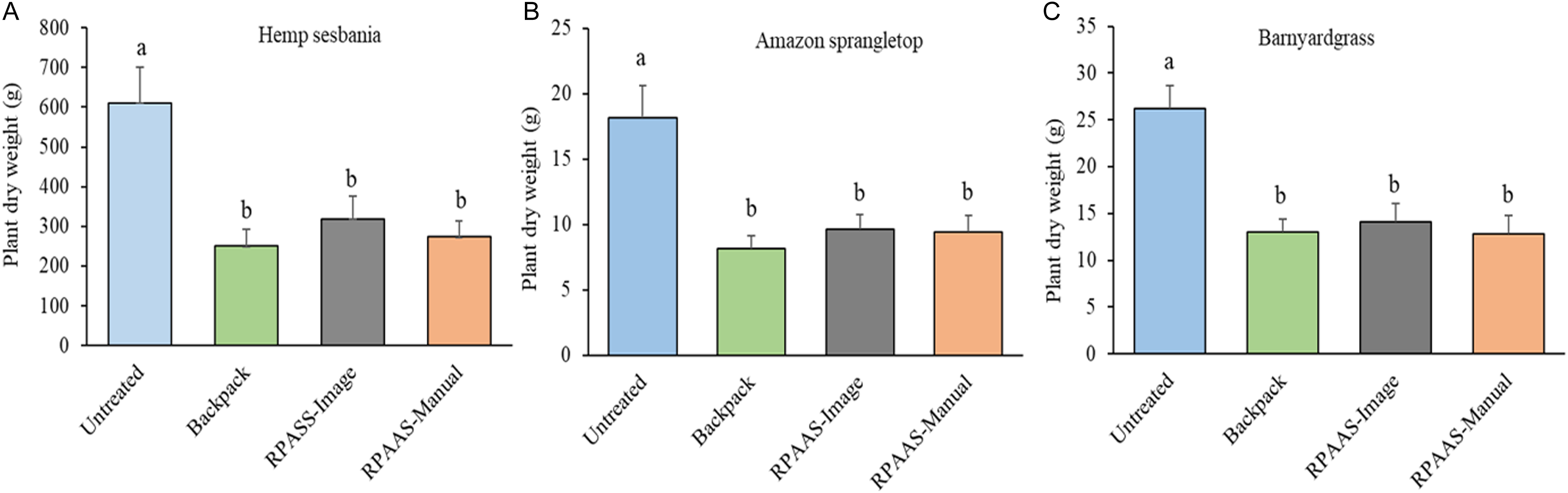
Figure 11. Impact of spray treatments on the dry biomass weight of hemp sesbania (A), Amazon sprangletop (B), and barnyardgrass (C) at 28 d after application. Biomass for yellow nutsedge could not be obtained due to rapid disintegration of the plants by the harvest date. The data were pooled across the two study years (Year × Treatment interaction was absent). The bars topped with different letters indicate significant differences based on Tukey’s HSD (α = 0.05). The whiskers on the bars represent standard errors of the mean.
Herbicide Volume Saving with RPAAS
The amount of herbicide used in site-specific applications varied between the two years and was influenced by weed density and spatial distribution. In 2021, there was a 45% reduction in herbicide volume for the RPAAS-based site-specific applications (both the manual geocoordinate method and the image-based geocoordinate method) compared to the backpack application. However, in 2022, weed density was higher compared to the previous year, resulting in only a 41% reduction in herbicide volume compared to the backpack method (Genna et al. Reference Genna, Gourlie and Barroso2021). These results align with Hunter et al. (Reference Hunter, Gannon, Richardson, Yelverton and Leon2020), in which a drone sprayer treated 20% to 60% less area than did ground-based broadcast application, with a 50% reduction in chemical volume (Hunter et al. Reference Hunter, Gannon, Richardson, Yelverton and Leon2020). However, the extent of herbicide volume reduction can also be influenced by factors like increased weed spatial patchiness and growth stage.
Droplet Spectrum and Deposition
A comparative analysis of droplet size and spray uniformity between the backpack and RPAAS systems revealed that the RPAAS sprays produced larger droplets with lower spray uniformity (P < 0.0001). The average VMD was greater for the RPAAS than for the backpack, measuring 1,800 μm and 1,077 μm, respectively. These differences were due to the differences in nozzle configurations associated with the two application methods (Table 3). This result was supported by Wolf and Daggupati (Reference Wolf and Daggupati2009), who stated that VMD is directly influenced by nozzle selection and operating pressure. Spray droplet uniformity, evaluated by the CV value, is another important factor that could be used to assess sprayer efficacy. A lower CV value indicates better droplet distribution, and vice versa, as demonstrated by Ferguson et al. (Reference Ferguson, O’Donnell, Chauhan, Adkins, Kruger, Wang, Ferreira and Hewitt2015). The results of our experiment show that the backpack treatments had a lower CV value (23.5%) than the RPAAS treatment (37%), indicating better spray uniformity across the experimental plots (P < 0.0001) (Figure 12 A). However, there was no significant difference in percentage spray coverage between RPAAS (17%) and backpack (22%) applications (P = 0.07) (Figure 12 B). The RPAAS droplets were larger than those from the backpack on the card, possibly due to downwash-caused droplet simmering (Figure 13), as well as the inherent differences in nozzle type (Table 3). These findings align with Martin et al. (Reference Martin, Woldt and Latheef2019), who reported that rotor downwash, along with the design and power ratings of RPAAS, could influence droplet distribution and uniformity.
Table 3. Droplet spectrum of remotely piloted aerial application system and backpack application methods. a,b
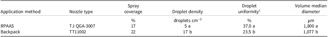
a Means followed by different letters within a column are significantly different according to Tukey’s HSD (α = 0.05).
b Abbreviation: RPAAS, remotely piloted aerial application system.
c Coefficient of variation.
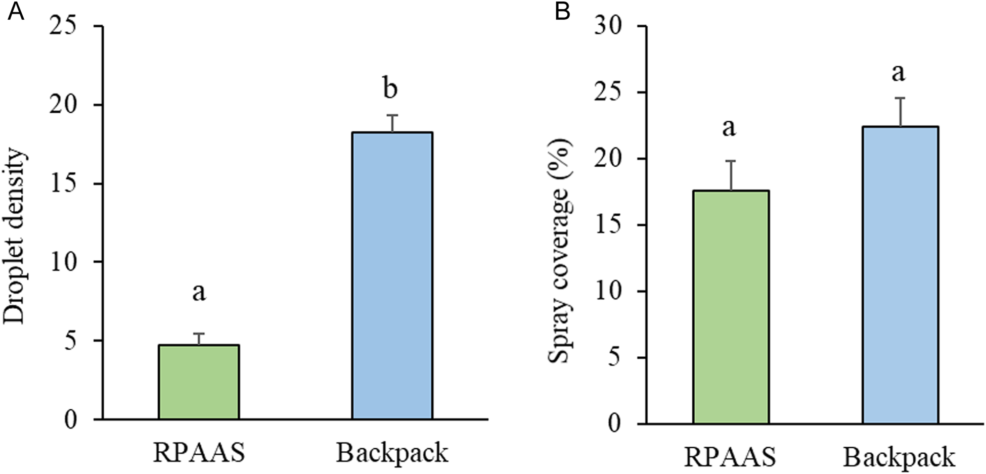
Figure 12 . Droplet density (droplets cm−2) (A) and spray coverage (%) (B) compared between the RPAAS and backpack application in a rice field. The data were pooled across the two study years (Year × Treatment interaction was absent). The bars topped with different letters indicate significant differences based on Tukey’s HSD (α = 0.05). The whiskers on the bars represent standard errors of the mean.
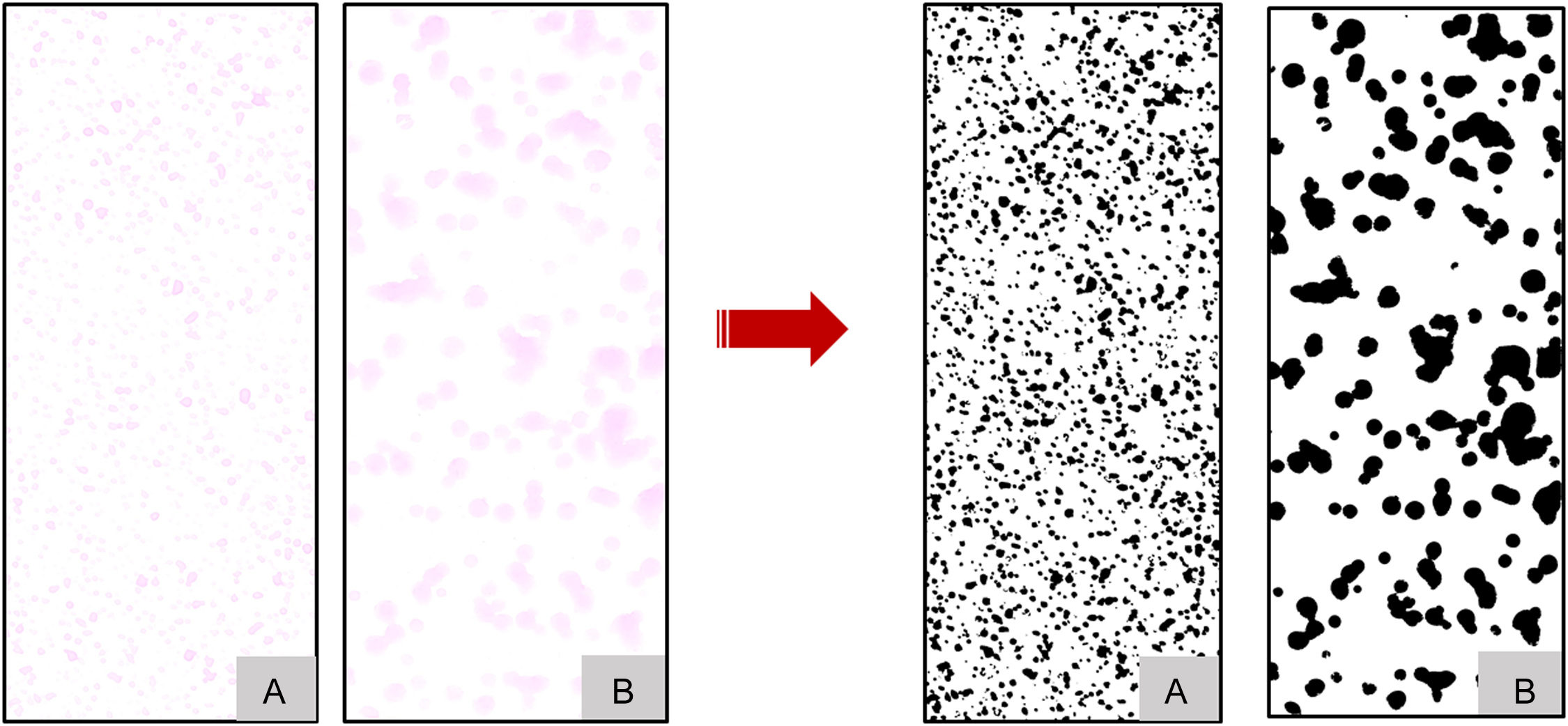
Figure 13. Raw (left) and processed (right) images of Kromekote cards, showing the spray coverage achieved by a backpack sprayer (A) and an RPAAS (B).
Rice Yield
Rice yield data revealed that RPAAS-based spot spraying is a better solution than traditional broadcast methods for late-season management of weed escapes. The broadcast application has caused unacceptable yield loss at the entire field level due to its adverse effects on rice during the reproductive development stages. For the RPAAS applications, on the other hand, the injury to rice was very localized only around the weed patches, leading to less crop damage at the field level. Figure 14 shows the rice yields measured in 2021 and 2022. Overall, the grain yield in 2022 was lower than in 2021 due to drought stress during panicle development. Rice yields were negatively influenced by the backpack (i.e., broadcast) herbicide application method (P < 0.0001), whereas the yields with the RPAAS-based site-specific applications were comparable to those of non-herbicide-treated plots. The majority of herbicides are not recommended for broadcast application up to 45 d before crop harvest due to the high risk of crop injury and the likelihood of unacceptable levels of chemical residues in the grain (FarmProgress 2023). However, RPAAS-based spot spraying can effectively manage late-season weed escapes and weed seed production without any significant adverse effects on rice yield because only a small area of the field is treated. Additionally, a spot spray application can reduce the amount of manpower and time needed to complete the task. Moreover, the RPAAS method is particularly convenient for areas that are difficult to reach from the ground (Sylvester Reference Sylvester2018), such as flooded rice paddies.
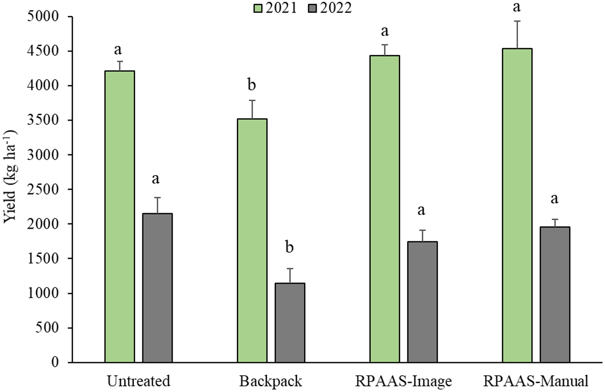
Figure 14. Comparison of rice grain yield (kg ha−1) between backpack application, RPAAS image-based geocoordinate method, RPAAS manual geocoordinate method, and untreated control for the two study years. The bars topped with different letters indicate significant differences based on Tukey’s HSD (α = 0.05). The whiskers on the bars represent standard errors of the mean.
Practical Implications
Overall, this study identified the potential for digital image processing and RPAAS for the site-specific control of late-season weeds that have emerged through a rice crop canopy. The combined approach of CHM and spectral signatures showed promise for the detection of late-season weed escapes using drone imagery. However, the weed recognition model exhibited suboptimal performance when the weed patches were at the same height as or smaller than the rice canopy or when there was no spectral signature difference between rice and the weed species. Although the traditional blanket ground application method, represented by the backpack technique in this study, remains the most effective for weed control, the RPAAS spray approach offers significant potential for herbicide savings and crop yield protection by precisely targeting weed-infested areas. Thus the RPAAS and image processing technology show great potential for limiting weed seed replenishment through the precise targeting of mid- to late-season weed escapes in rice crops, contributing to more sustainable weed management practices. Additionally, this technology enhances the efficiency of herbicides while minimizing crop injury, which is an important consideration for late-season applications for which the potential for herbicide residue in grains is a serious concern. Moreover, the agility of RPAAS enables it to navigate challenging or flooded fields that may be difficult for ground-based methods to access. Furthermore, the RPAAS method can assist rice growers in controlling weeds efficiently and in a timely manner through site-specific application. Future research should focus on integrating CHM, spectral signatures, and texture information of both crop and weeds to improve species differentiation. Exploring machine learning–based approaches for weed detection and localization may hold promise for addressing the challenges identified in this study. Future research should also focus on identifying optimal spraying parameters that improve deposition uniformity for the control of late-season weed escapes in rice. These parameters include nozzle type, application height, wind effects, and the required chemical quantities for effective weed control.
Acknowledgments
The authors acknowledge Jason Samford and the field staff at the David Wintermann Rice Research and Extension Center, Eagle Lake, TX for helping with field establishment and maintenance.
Funding
This research was funded in part by the Texas Rice Research Foundation and the USDA-Natural Resources Conservation Service-Conservation Innovation Grant (award #: NR213A750013G017). BG acknowledges a graduate fellowship from the Nethaji-Subhash International Fellowship Program of the Indian Government.
Competing interests
The authors declare no conflicts of interest.


 Open access