


1 Introduction
Factor analysis is a popular technique for learning the underlying structure of multivariate data and has wide applications in psychology and the social sciences. Factor analysis suffers from the rotational indeterminacy issue where the loading matrix and the factors can be simultaneously rotated under the same model. The rotation procedure is a crucial step in obtaining an interpretable structure. The prevailing solution seeks the rotation that renders a simple structure (Thurstone, Reference Thurstone1947). Roughly speaking, Thurstone’s simple structure means that the loading matrix contains as many (approximately) zero entries as possible, so that each observed variable can be explained by only a few factors. Nevertheless, the simple structure is not the only desired solution, especially when the result does not admit a perfect simple structure. The bi-factor analysis, for instance, has become a popular alternative solution for exploring the factor structure (Reise, Reference Reise2012). A classic approach to the bi-factor analysis is the Schmid–Leiman (SL; Schmid & Leiman, Reference Schmid and Leiman1957) transformation. However, the SL transformation imposes an unnecessary proportionality constraint, making the loading matrix inevitably rank-deficient (Waller, Reference Waller2018). Moreover, the SL transformation only produces orthogonal factors, leaving the oblique bi-factor analysis unsolved. Recently, some new strategies have been developed for bi-factor analysis (Abad et al., Reference Abad, Garcia-Garzon, Garrido and Barrada2017; Jennrich & Bentler, Reference Jennrich and Bentler2011, Reference Jennrich and Bentler2012), but their performance has not been thoroughly discussed, and none of them has been accepted as the conventional approach.
This article attempts to shed some light on the bi-factor rotation problem, and more generally, on the factor rotation problem. We provide a mathematical framework to formulate and solve the rotation problem (both orthogonal and oblique) in factor analysis. Given any desired property of the factor structure, our framework incorporates it as a penalty term or a constraint, and by solving an optimization problem, it produces a rotation that rotates an initial loading matrix toward the desired property. In the bi-factor analysis, for example, the rotated loading matrix is expected to have a bi-factor structure. Accordingly, our framework takes the bi-factor structure as a constraint and produces a rotation that rotates an initial loading matrix into a bi-factor matrix as much as possible. We also provide a convergent algorithm to solve the optimization problem. Jennrich (Reference Jennrich2001, Reference Jennrich2002) has devised a gradient-based algorithm for optimizing a general rotation criterion function, which generates a sequence of monotone iterates. However, the monotone iterates only guarantee the convergence of some subsequence, and there might exist multiple limiting points. Indeed, the monotone iterates may oscillate indefinitely and generate paths with infinite length (see Absil et al., Reference Absil, Mahony and Andrews2005 for such an example). In contrast, our algorithm guarantees the convergence of the whole iterates.
Although the problem of simple structure rotation has been extensively studied, we still demonstrate the utilization of our framework in solving this problem, partly because it serves as an example of the penalty-type formulation and partly because it provides a new perspective (and a new algorithm) on solving this problem. Thurstone’s original concept of simple structure largely concerns the number of zero loadings, but many existing methods maximize some dispersion of factor loadings so that the loadings tend to be either very high or very low. As Nesselroade and Cattell (Reference Nesselroade and Cattell2013) note, “the position that gives merely a lot of low loadings is different from the exact one that maximizes the number of zero loadings.” Moreover, these dispersion-based methods raise the scaling issues, such as sensitivity to outliers and the question of normalization. In contrast, our framework provides a solution on the basis of the count of zero/nonzero loadings, agreeing with the very notion of simple structure.
We emphasize that our framework is not limited to the simple structure or bi-factor rotations. The regularization term in our framework can be customized to represent any subjective or theoretical assumptions about the factor structure, and our framework identifies the optimal rotation solution corresponding to the given assumption. This is an attractive advantage because researchers may have various demands on the exploratory factor analysis (EFA) across different applications. This regularized formulation also provides a perspective to unify the rotation procedure and the penalized estimation. We justify in Section 6.2 that these two seemingly competing procedures are mathematically almost equivalent.
The remainder of this article is organized as follows. Section 2 and Section 3 describe our framework for solving the orthogonal and oblique rotation problems, respectively. In each section, we demonstrate both the simple structure rotation and the bi-factor rotation, along with their algorithms. In Section 4, we conduct a simulation to compare the performance of our framework in the exploratory bi-factor analysis with existing methods. The proposed method is applied to real datasets in Section 5. Section 6 discusses some connections between our framework and other methods. Section 7 concludes this article. Technical derivations and proofs are postponed to the Appendix, which also includes supplementary simulation studies.
2 Orthogonal rotation
2.1 Rotation to simple structure
Let $A \in \mathbb {R}^{p \times k}$
be an initial loading matrix and
$A \in \mathbb {R}^{p \times k}$
be an initial loading matrix and $T \in \mathbb {R}^{k \times k}$
an orthogonal matrix. The concept of simple structure in factor analysis concerns the search of T such that
$T \in \mathbb {R}^{k \times k}$
an orthogonal matrix. The concept of simple structure in factor analysis concerns the search of T such that $AT$
is as simple as possible. If simplicity is defined as the number of zero loadings, a natural choice is to minimize
$AT$
is as simple as possible. If simplicity is defined as the number of zero loadings, a natural choice is to minimize $\| AT \|_0$
, where
$\| AT \|_0$
, where $\| \cdot \|_0$
counts the number of nonzero entries. Unfortunately,
$\| \cdot \|_0$
counts the number of nonzero entries. Unfortunately, $AT$
would not contain many exact zeros in general, especially when the loading matrix is subject to sampling error. In practice, very small loadings are accepted as zeros. In other words,
$AT$
would not contain many exact zeros in general, especially when the loading matrix is subject to sampling error. In practice, very small loadings are accepted as zeros. In other words, $AT$
would be considered simple if it is close to some matrix with many zeros. Thus, we formulate the objective function as
$AT$
would be considered simple if it is close to some matrix with many zeros. Thus, we formulate the objective function as
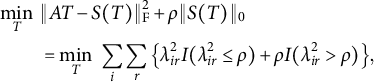
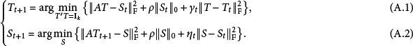
 $$ \begin{align} \begin{aligned} \min_{T,S}&~ \|AT - S\|_{\mathrm{F}}^2 + \rho \|S\|_0, \\ \mathrm{s.t.} &~ T'T = \mathbf{I}_k, \end{aligned} \end{align} $$
where $\| \cdot \|_{\mathrm {F}}$
is the Frobenius norm,
$\| \cdot \|_{\mathrm {F}}$
is the Frobenius norm, $\rho>0$
is the tuning parameter, the prime denotes matrix transpose, and
$\rho>0$
is the tuning parameter, the prime denotes matrix transpose, and $\mathbf {I}_k$
is the k-by-k identity matrix. In practice, we use
$\mathbf {I}_k$
is the k-by-k identity matrix. In practice, we use $\rho =0.3^2$
, and this choice will be explained in Section 6.1.
$\rho =0.3^2$
, and this choice will be explained in Section 6.1.
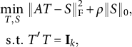
2.2 Algorithm
Our objective function (2.1) introduces a new parameter S and seems to be more difficult to optimize than the usual criteria that involve only a rotation parameter T. However, we shall show that the introduction of a new parameter not only simplifies the optimization but also broadens its applicability. The key is the separation of the rotation constraint (on T) and the desired property (on S). The usual approaches consider the desired sparsity or its surrogate criterion directly on the rotated loadings, the interlock of which makes the factor rotation problem challenging. In (2.1) these two features are individually applied to T and to S, and they are linked by a simple Frobenius distance function. This makes the optimization with respect to each parameter very simple. While this might suggest applying an alternating minimization algorithm to solve (2.1), this algorithm suffers from the same drawback as the gradient-based algorithm: the sequence of parameters generated by the algorithm is not guaranteed to converge (Powell, Reference Powell1973). Therefore, a convergent algorithm called the proximal alternating minimization (PAM) algorithm (Attouch et al., Reference Attouch, Bolte, Redont and Soubeyran2010) is employed to solve (2.1).
If $X=UDV'$
is the singular value decomposition of X, then
$X=UDV'$
is the singular value decomposition of X, then $T=UV'$
minimizes
$T=UV'$
minimizes $\|X- T\|_{\mathrm {F}}^2$
subject to
$\|X- T\|_{\mathrm {F}}^2$
subject to $T'T=TT'=\mathbf {I}_k$
(Gower & Dijksterhuis, Reference Gower and Dijksterhuis2004). We denote this projection by
$T'T=TT'=\mathbf {I}_k$
(Gower & Dijksterhuis, Reference Gower and Dijksterhuis2004). We denote this projection by $\mathcal {P}_{\mathrm {orth}} (X) = UV'$
. Let
$\mathcal {P}_{\mathrm {orth}} (X) = UV'$
. Let $\mathcal {H}(X, \kappa ) = X \circ I(|X|> \kappa )$
be the entrywise hard-thresholding operator for a matrix X, where
$\mathcal {H}(X, \kappa ) = X \circ I(|X|> \kappa )$
be the entrywise hard-thresholding operator for a matrix X, where $\circ $
is the entrywise matrix product and
$\circ $
is the entrywise matrix product and $I ( |X|> \kappa )$
is the entrywise indicator function for whether the absolute value of X entries is greater than a scalar threshold
$I ( |X|> \kappa )$
is the entrywise indicator function for whether the absolute value of X entries is greater than a scalar threshold $\kappa $
. The algorithm is presented in Algorithm 1, which updates T and S alternately using the above operators (see Appendix A.1 for the derivation). The convergence result of this algorithm is summarized in Proposition 1, whose proof is given in Appendix A.2. The algorithm converges to a stationary pointFootnote 1 for any bounded stepsizes
$\kappa $
. The algorithm is presented in Algorithm 1, which updates T and S alternately using the above operators (see Appendix A.1 for the derivation). The convergence result of this algorithm is summarized in Proposition 1, whose proof is given in Appendix A.2. The algorithm converges to a stationary pointFootnote 1 for any bounded stepsizes $\gamma _t$
and
$\gamma _t$
and $\eta _t$
. In practice, we choose some small values, such as
$\eta _t$
. In practice, we choose some small values, such as $\gamma _t = \eta _t = 0.01$
. Also worth mentioning is the issue of local minima. Like many other rotation methods, Algorithm 1 may converge to a local minimum because the rotation problem is non-convex. Therefore, it is recommended to run the algorithm with multiple random initializations and choose the one with the smallest objective value.
$\gamma _t = \eta _t = 0.01$
. Also worth mentioning is the issue of local minima. Like many other rotation methods, Algorithm 1 may converge to a local minimum because the rotation problem is non-convex. Therefore, it is recommended to run the algorithm with multiple random initializations and choose the one with the smallest objective value.
Proposition 1. Assume that the sequences of stepsizes $\gamma _t$
and
$\gamma _t$
and $\eta _t$
are bounded away from zero and infinity, that is, there exists some positive numbers
$\eta _t$
are bounded away from zero and infinity, that is, there exists some positive numbers $r_+> r_- >0$
such that
$r_+> r_- >0$
such that $\gamma _t, \eta _t$
belong to
$\gamma _t, \eta _t$
belong to $(r_-, r_+)$
for all
$(r_-, r_+)$
for all $t\geq 0$
. Then the iterates
$t\geq 0$
. Then the iterates $(T_t, S_t)$
generated by Algorithm 1 converge to a stationary point of (2.1).
$(T_t, S_t)$
generated by Algorithm 1 converge to a stationary point of (2.1).
2.3 Bi-factor rotation
In the simple structure rotation, we maximize the degree of simplicity for the loading matrix, so our framework formulates the problem as a penalized optimization. When the loading matrix is desired to satisfy certain restrictions, we formulate it as a constrained problem, which can also be efficiently solved by the PAM algorithm. An example of such a problem is the exploratory bi-factor analysis.
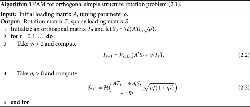
A bi-factor model has a loading matrix of the form
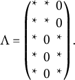 $$\begin{align*}\Lambda = \begin{pmatrix} * & * & 0 \\ * & * & 0 \\ * & 0 & * \\ * & 0 & * \\ * & 0 & * \end{pmatrix}. \end{align*}$$
Formally speaking, the loading matrix has a column of free parameters, and besides this column, it has at most one free parameter in each row. The factor corresponding to the free column is called a general factor, and the remaining factors are called group factors. Exploratory bi-factor analysis (Jennrich & Bentler, Reference Jennrich and Bentler2011; Reise, Reference Reise2012) can uncover the bi-factor structure and estimate the loadings simultaneously, unlike the confirmatory bi-factor analysis that requires the bi-factor structure to be specified in advance. Let $\mathcal {S}_{\mathrm {bi}}$
denote the set of matrices with bi-factor structure. Our method performs exploratory bi-factor analysis by solving
$\mathcal {S}_{\mathrm {bi}}$
denote the set of matrices with bi-factor structure. Our method performs exploratory bi-factor analysis by solving
 $$ \begin{align} \begin{aligned} \min_{T,S}&~ \|AT - S\|_{\mathrm{F}}^2, \cr \mathrm{s.t.} &~ T'T = \mathbf{I}_k, \: S \in \mathcal{S}_{\mathrm{bi}}. \end{aligned} \end{align} $$
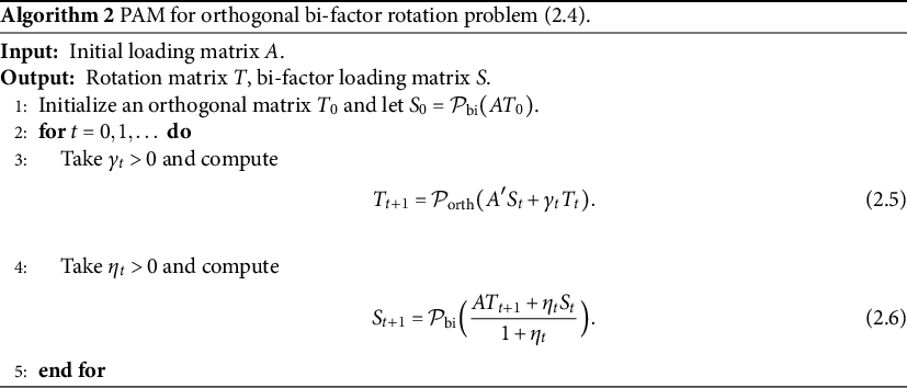
The algorithm for solving (2.4) is very similar to Algorithm 1 and is presented in Algorithm 2. It involves the projection operator onto bi-factor matrices $\mathcal {P}_{\mathrm {bi}}(X) := \mathrm {arg} \min _{S \in \mathcal {S}_{\mathrm {bi}}} \|S - X \|_{\mathrm {F}}$
. The evaluation of this projection requires solving a simple combinatorial optimization to find the column of general factor loadings and then keeping the largest (in absolute value) entry in each row of the remaining columns as the group factor loadings (see Appendix A.3 for a detailed description).
$\mathcal {P}_{\mathrm {bi}}(X) := \mathrm {arg} \min _{S \in \mathcal {S}_{\mathrm {bi}}} \|S - X \|_{\mathrm {F}}$
. The evaluation of this projection requires solving a simple combinatorial optimization to find the column of general factor loadings and then keeping the largest (in absolute value) entry in each row of the remaining columns as the group factor loadings (see Appendix A.3 for a detailed description).
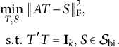
3 Oblique rotation
3.1 Rotation to simple structure
In the orthogonal rotation case, the factors are uncorrelated, and the rotation matrix is restricted to be an orthogonal matrix. When the factors are allowed to be correlated, the oblique rotation problem arises. This section provides a counterpart of our framework to solve the oblique rotation problem, which is similar to the orthogonal case but has some subtle yet crucial differences.
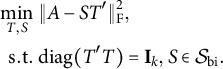
If one is primarily interested in the loading matrix estimation, the oblique version of the simple structure rotation problem might be formulated as
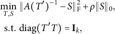 $$ \begin{align} \begin{aligned} \min_{T,S}&~ \|A(T')^{-1} - S\|_{\mathrm{F}}^2 + \rho \|S\|_0, \cr \mathrm{s.t.} &~ \mathrm{diag} (T'T) = \mathbf{I}_k, \end{aligned} \end{align} $$
where $\mathrm {diag} (\cdot )$
keeps the diagonal part of a matrix and assigns zeros to the off-diagonal part, as (3.1) finds the rotated loading matrix
$\mathrm {diag} (\cdot )$
keeps the diagonal part of a matrix and assigns zeros to the off-diagonal part, as (3.1) finds the rotated loading matrix $A(T')^{-1}$
that is closest to a hypothesized simple loading matrix S. However, in the oblique factor analysis, the factor correlation matrix also needs to be estimated, and the rotation T is responsible for both the loading matrix
$A(T')^{-1}$
that is closest to a hypothesized simple loading matrix S. However, in the oblique factor analysis, the factor correlation matrix also needs to be estimated, and the rotation T is responsible for both the loading matrix $A(T')^{-1}$
and the factor correlation matrix
$A(T')^{-1}$
and the factor correlation matrix $\Phi = T'T$
. In order to get an overall better estimation of the loading matrix and the factor correlation matrix, we propose to formulate the oblique rotation problem as
$\Phi = T'T$
. In order to get an overall better estimation of the loading matrix and the factor correlation matrix, we propose to formulate the oblique rotation problem as
 $$ \begin{align} \begin{aligned} \min_{T,S}&~ \|A - S T'\|_{\mathrm{F}}^2 + \rho \|S\|_0, \cr \mathrm{s.t.} &~ \mathrm{diag} (T'T) = \mathbf{I}_k. \end{aligned} \end{align} $$
When $\|A - S T'\|_{\mathrm {F}}$
is minimized, the reproduced covariance matrix
$\|A - S T'\|_{\mathrm {F}}$
is minimized, the reproduced covariance matrix $A(T')^{-1}\Phi T^{-1}A' + \Psi ^2 = AA' + \Psi ^2$
will be close to the hypothesized covariance matrix
$A(T')^{-1}\Phi T^{-1}A' + \Psi ^2 = AA' + \Psi ^2$
will be close to the hypothesized covariance matrix $ST'TS' + \Psi ^2$
with a simple loading matrix S, where
$ST'TS' + \Psi ^2$
with a simple loading matrix S, where $\Psi ^2$
is a diagonal matrix of uniqueness. As the covariance matrix is governed by the loading matrix and factor correlation matrix, achieving closeness in the covariance matrix facilitates a balanced estimation of these two parameters. The rotated loading matrix
$\Psi ^2$
is a diagonal matrix of uniqueness. As the covariance matrix is governed by the loading matrix and factor correlation matrix, achieving closeness in the covariance matrix facilitates a balanced estimation of these two parameters. The rotated loading matrix $A(T')^{-1}$
will be approximately simple since
$A(T')^{-1}$
will be approximately simple since $A(T')^{-1} \approx ST'(T')^{-1} = S$
; the factor correlation matrix
$A(T')^{-1} \approx ST'(T')^{-1} = S$
; the factor correlation matrix $\Phi = T'T$
is suitable for the hypothesized simple structure since
$\Phi = T'T$
is suitable for the hypothesized simple structure since $ST'TS' + \Psi ^2$
is close to the optimal covariance matrix
$ST'TS' + \Psi ^2$
is close to the optimal covariance matrix $AA' + \Psi ^2$
. The advantages of (3.2) in estimating the correlation matrix will be numerically illustrated in Section 4 and Appendix A.7.
$AA' + \Psi ^2$
. The advantages of (3.2) in estimating the correlation matrix will be numerically illustrated in Section 4 and Appendix A.7.
This nuance does not appear in the orthogonal rotation problem because the orthogonal factor correlation matrix is invariant and the rotation is only responsible for the loading matrix. In effect, for an orthogonal matrix T, $\|A-ST'\|_{\mathrm {F}} = \|(A-ST')T\|_{\mathrm {F}} = \|AT-S\|_{\mathrm {F}}$
, so the two formulations are equivalent.
$\|A-ST'\|_{\mathrm {F}} = \|(A-ST')T\|_{\mathrm {F}} = \|AT-S\|_{\mathrm {F}}$
, so the two formulations are equivalent.
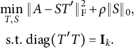
As for the algorithm, although the alternating minimization algorithm and the PAM algorithm are conceptually applicable to (3.2), they do not lead to a practical algorithm because the iteration steps for problem (3.2) do not bear explicit updating formulas with these algorithms. We employ the proximal alternating linearized minimization (PALM) algorithm (Bolte et al., Reference Bolte, Sabach and Teboulle2014) to solve (3.2). The resulting algorithm is reported in Algorithm 3. The projection onto oblique rotation matrices $\mathcal {P}_{\mathrm {oblq}} (X) = X\{\mathrm {diag}(X'X)\}^{-1/2}$
rescales each column of matrix X to unit length. We use an orthogonal matrix as initialization because, in general, it has empirically better performance than an oblique one. In practice, we choose the values of
$\mathcal {P}_{\mathrm {oblq}} (X) = X\{\mathrm {diag}(X'X)\}^{-1/2}$
rescales each column of matrix X to unit length. We use an orthogonal matrix as initialization because, in general, it has empirically better performance than an oblique one. In practice, we choose the values of $\gamma $
and
$\gamma $
and $\eta $
slightly above one, such as
$\eta $
slightly above one, such as $\gamma = \eta = 1.01$
. This algorithm is also convergent, as recorded in Proposition 2 with proof given in Appendix A.5. It is again recommended to run the algorithm multiple times to alleviate the issue of local minima.
$\gamma = \eta = 1.01$
. This algorithm is also convergent, as recorded in Proposition 2 with proof given in Appendix A.5. It is again recommended to run the algorithm multiple times to alleviate the issue of local minima.


3.2 Bi-factor rotation
As in the orthogonal case, formulation (3.2) and the PALM algorithm can be used for other purposes in oblique rotation. We continue to demonstrate the exploratory bi-factor analysis because it highlights some new issues in the oblique case. We shall show that the bi-factor model suffers from what we would call group-factor indeterminacy when the factors are allowed to be correlated. This indeterminacy can be suppressed if we restrict all the group factors to be uncorrelated with the general factor.
The group-factor indeterminacy is illustrated as follows. Let $\Lambda \in \mathbb {R}^{p \times k}$
be a bi-factor loading matrix and
$\Lambda \in \mathbb {R}^{p \times k}$
be a bi-factor loading matrix and $\boldsymbol {F} \in \mathbb {R}^k$
the corresponding factors. Without loss of generality, we let the first component in
$\boldsymbol {F} \in \mathbb {R}^k$
the corresponding factors. Without loss of generality, we let the first component in $\boldsymbol {F}$
be the general factor. Let
$\boldsymbol {F}$
be the general factor. Let $\Phi = (\phi _{ij}) \in \mathbb {R}^{k \times k}$
be the factor correlation matrix. Construct a transformation matrix
$\Phi = (\phi _{ij}) \in \mathbb {R}^{k \times k}$
be the factor correlation matrix. Construct a transformation matrix $\Gamma \in \mathbb {R}^{k \times k}$
as
$\Gamma \in \mathbb {R}^{k \times k}$
as
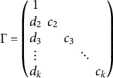 $$ \begin{align} \Gamma = \begin{pmatrix} 1 & & & & \\ d_2 & c_2 & & & \\ d_3 & & c_3 & & \\ \vdots & & & \ddots & \\ d_k & & & & c_k \end{pmatrix} \end{align} $$
that has zeros at locations other than the main diagonal and the first column. Matrix $\Gamma $
has an inverse
$\Gamma $
has an inverse
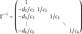 $$\begin{align*}\Gamma^{-1} = \begin{pmatrix} 1 & & & & \\ -d_2/c_2 & 1/c_2 & & & \\ -d_3/c_3 & & 1/c_3 & & \\ \vdots & & & \ddots & \\ -d_k/c_k & & & & 1/c_k \end{pmatrix} \end{align*}$$
whenever it exists. The transformed factor $\widetilde {\boldsymbol {F}} = \Gamma \boldsymbol {F}$
has a covariance matrix
$\widetilde {\boldsymbol {F}} = \Gamma \boldsymbol {F}$
has a covariance matrix $\Gamma \Phi \Gamma '$
, whose diagonal elements are
$\Gamma \Phi \Gamma '$
, whose diagonal elements are $d_r^2 + 2 c_r \phi _{1r} d_r + c_r^2$
(except for the first one). We set
$d_r^2 + 2 c_r \phi _{1r} d_r + c_r^2$
(except for the first one). We set $d_r = -c_r \phi _{1r}\pm \sqrt {1 - c_r^2(1-\phi _{1r}^2)}$
for all
$d_r = -c_r \phi _{1r}\pm \sqrt {1 - c_r^2(1-\phi _{1r}^2)}$
for all $2 \leq r \leq k$
, so that the transformed factor is standardized. The
$2 \leq r \leq k$
, so that the transformed factor is standardized. The $c_r$
can be any nonzero number between
$c_r$
can be any nonzero number between $-1/\sqrt {1-\phi _{1r}^2}$
and
$-1/\sqrt {1-\phi _{1r}^2}$
and $1/\sqrt {1-\phi _{1r}^2}$
. The transformed loading matrix
$1/\sqrt {1-\phi _{1r}^2}$
. The transformed loading matrix $\widetilde {\Lambda } = \Lambda \Gamma ^{-1}$
has the same bi-factor structure as
$\widetilde {\Lambda } = \Lambda \Gamma ^{-1}$
has the same bi-factor structure as $\Lambda $
. Thus, we have constructed a different oblique bi-factor representation
$\Lambda $
. Thus, we have constructed a different oblique bi-factor representation $\widetilde {\Lambda } \widetilde {\boldsymbol {F}} = \Lambda \boldsymbol {F}$
. Intuitively, each cluster of items indicated by the group factors forms a micro factor model with two common factors (the general factor and the corresponding group factor). Under the oblique factor case, the group factor can be rotated toward or against the general factor within this two-factor model (we should not rotate the general factor because it is shared by other clusters). This explains how we construct the transformation matrix
$\widetilde {\Lambda } \widetilde {\boldsymbol {F}} = \Lambda \boldsymbol {F}$
. Intuitively, each cluster of items indicated by the group factors forms a micro factor model with two common factors (the general factor and the corresponding group factor). Under the oblique factor case, the group factor can be rotated toward or against the general factor within this two-factor model (we should not rotate the general factor because it is shared by other clusters). This explains how we construct the transformation matrix $\Gamma $
, and we call this phenomenon group-factor indeterminacy of the oblique bi-factor model. This result is not new and has been disclosed by Jennrich and Bentler (Reference Jennrich and Bentler2012). A natural yet putative strategy to resolve this indeterminacy is to restrict the group factors to be uncorrelated with the general factor. We call such a bi-factor representation a semi-oblique bi-factor model. A fully oblique bi-factor representation can be transformed into a semi-oblique one using
$\Gamma $
, and we call this phenomenon group-factor indeterminacy of the oblique bi-factor model. This result is not new and has been disclosed by Jennrich and Bentler (Reference Jennrich and Bentler2012). A natural yet putative strategy to resolve this indeterminacy is to restrict the group factors to be uncorrelated with the general factor. We call such a bi-factor representation a semi-oblique bi-factor model. A fully oblique bi-factor representation can be transformed into a semi-oblique one using $\Gamma $
with
$\Gamma $
with $c_r = 1/\sqrt {1-\phi _{1r}^2}$
and
$c_r = 1/\sqrt {1-\phi _{1r}^2}$
and $d_r = -c_r \phi _{1r}$
for all
$d_r = -c_r \phi _{1r}$
for all $2 \leq r \leq k$
.
$2 \leq r \leq k$
.
Even given the indeterminacy and the putative restriction, we can still formulate and solve the oblique exploratory bi-factor analysis with
 $$ \begin{align} \begin{aligned} \min_{T,S}&~ \|A - S T'\|_{\mathrm{F}}^2, \cr \mathrm{s.t.} &~ \mathrm{diag}(T'T) = \mathbf{I}_k, \: S \in \mathcal{S}_{\mathrm{bi}}. \end{aligned} \end{align} $$
It should be clarified that the fully oblique bi-factor models are not considered false or invalid. They are different representations of the equivalent bi-factor models. In effect, this indeterminacy does not affect the feasibility $S \in \mathcal {S}_{\mathrm {bi}}$
and the objective value
$S \in \mathcal {S}_{\mathrm {bi}}$
and the objective value $\|A - S T'\|_{\mathrm {F}}^2$
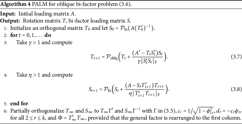
. Consequently, (3.6) has a continuum of optimal solutions that correspond to a single model, and we transform the final result into a semi-oblique one to provide a unique representation.Footnote 2 Hence, Algorithm 4 solves the oblique bi-factor problem with the PALM algorithm, followed by a partial orthogonalization step.
$\|A - S T'\|_{\mathrm {F}}^2$
. Consequently, (3.6) has a continuum of optimal solutions that correspond to a single model, and we transform the final result into a semi-oblique one to provide a unique representation.Footnote 2 Hence, Algorithm 4 solves the oblique bi-factor problem with the PALM algorithm, followed by a partial orthogonalization step.
4 Simulation
We have proposed a general framework to formulate and solve the rotation problem in factor analysis and demonstrated it through the examples of simple structure rotation and exploratory bi-factor analysis. Because the simple structure rotation problem has been extensively studied and mature solutions have been developed, our simulation experience shows considerable similarity between our method and the existing popular methods in terms of numerical performance (see Appendix A.6 for the simulation results). Here, we exhibit the simulation results for the exploratory bi-factor analysis. The R code for running the simulations and conducting the analyses are available in the online supplemental materials.
We compare our proposed method with eight existing methods: (a) the SL (the Schmid-Leiman procedure; Schmid & Leiman, Reference Schmid and Leiman1957); (b) the SLt (the SL followed by a partially specified target rotation; Reise et al., Reference Reise, Moore and Haviland2010); (c) the SLi (the SL followed by iterated target rotations; Abad et al., Reference Abad, Garcia-Garzon, Garrido and Barrada2017); (d) the DSL (the Direct Schmid-Leiman method; Waller, Reference Waller2018); (e) the DBF (the Direct Bi-Factor method; Waller, Reference Waller2018); (f) the PEBI (the orthogonal or oblique Pure Exploratory BI-factor analysis; Lorenzo-Seva & Ferrando, Reference Lorenzo-Seva and Ferrando2019); (g) the BQ.orth (the orthogonal Bi-Quartimin method; Jennrich & Bentler, Reference Jennrich and Bentler2011); and (h) the BQ.oblq (the oblique Bi-Quartimin method; Jennrich & Bentler, Reference Jennrich and Bentler2012). We basically follow the simulation settings from Abad et al. (Reference Abad, Garcia-Garzon, Garrido and Barrada2017) and Giordano and Waller (Reference Giordano and Waller2020). Specifically, we consider a total of $22$
items clustered into four groups, with four, five, six, and seven items in each group. We examine four types of bi-factor structures: (a) the independent cluster (IC) structure that is a perfect bi-factor loading matrix; (b) the independent cluster basis (ICB) structure that contains cross-loadings; (c) the independent cluster pure (ICP) structure where some items have nonzero loadings only on the general factor; and (d) the independent cluster basis pure (ICBP) structure that contains both cross-loadings and pure items. In our simulation, the group factor loadings take either high or low values. When they take high values, they are randomly selected from the interval
$22$
items clustered into four groups, with four, five, six, and seven items in each group. We examine four types of bi-factor structures: (a) the independent cluster (IC) structure that is a perfect bi-factor loading matrix; (b) the independent cluster basis (ICB) structure that contains cross-loadings; (c) the independent cluster pure (ICP) structure where some items have nonzero loadings only on the general factor; and (d) the independent cluster basis pure (ICBP) structure that contains both cross-loadings and pure items. In our simulation, the group factor loadings take either high or low values. When they take high values, they are randomly selected from the interval $[0.6,0.9]$
; for the low value case, they are selected from the range
$[0.6,0.9]$
; for the low value case, they are selected from the range $[0.3,0.6]$
. When cross-loadings are present, the last item in each cluster has a cross-loading of
$[0.3,0.6]$
. When cross-loadings are present, the last item in each cluster has a cross-loading of $0.4$
on the next group factor. For pure items, the item in the middle position of each cluster has a loading of
$0.4$
on the next group factor. For pure items, the item in the middle position of each cluster has a loading of $0.01$
on the corresponding group factor. The loadings on the general factor are randomly selected so that every item has communality no greater than
$0.01$
on the corresponding group factor. The loadings on the general factor are randomly selected so that every item has communality no greater than $0.81$
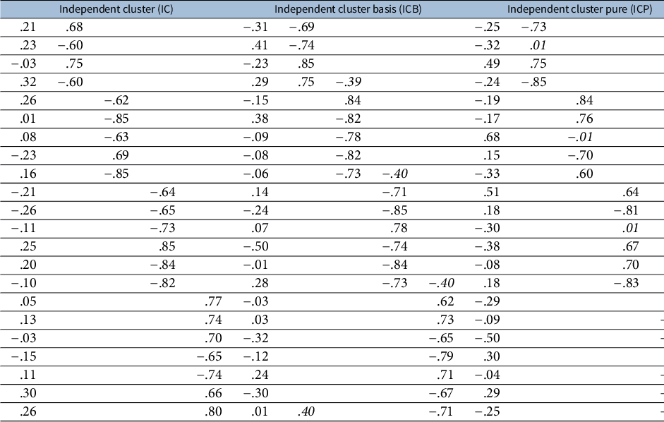
. When necessary, some rows of loading vector are rescaled to prevent excessively large communality caused by the cross-loadings. Finally, every loading entry is randomly assigned a positive or negative sign. An example of simulated loading matrices is presented in Table 1.
$0.81$
. When necessary, some rows of loading vector are rescaled to prevent excessively large communality caused by the cross-loadings. Finally, every loading entry is randomly assigned a positive or negative sign. An example of simulated loading matrices is presented in Table 1.
Table 1 Examples of the loading matrix under the four types of bi-factor structure
Given the simulated loading matrix $\Lambda $
, we generate the population correlation matrix
$\Lambda $
, we generate the population correlation matrix
 $$\begin{align*}R = \Lambda \Phi \Lambda' + \Psi^2, \end{align*}$$
where $\Phi $
is the factor correlation matrix and
$\Phi $
is the factor correlation matrix and $\Psi ^2$
is a diagonal matrix of uniqueness, chosen to constrain the diagonal elements of R to one. In the orthogonal bi-factor case,
$\Psi ^2$
is a diagonal matrix of uniqueness, chosen to constrain the diagonal elements of R to one. In the orthogonal bi-factor case, $\Phi $
will be an identity matrix. In the semi-oblique case, the correlations among group factors are randomly selected from the interval
$\Phi $
will be an identity matrix. In the semi-oblique case, the correlations among group factors are randomly selected from the interval $[0.2, 0.6]$
. If the generated correlation matrix is not positive definite, we re-generate a new one until it is positive definite. The final step generates the data from a multivariate normal distribution with zero mean and covariance matrix R, with a sample size
$[0.2, 0.6]$
. If the generated correlation matrix is not positive definite, we re-generate a new one until it is positive definite. The final step generates the data from a multivariate normal distribution with zero mean and covariance matrix R, with a sample size $N \in \{200, 500, 2000\}$
. The simulation is replicated
$N \in \{200, 500, 2000\}$
. The simulation is replicated $50$
times for each scenario.
$50$
times for each scenario.
The accuracy of the rotation methods is evaluated by the root mean squared error (RMSE) between the population and estimated bi-factor loading matrices:
 $$ \begin{align} \mathrm{RMSE} ( \Lambda, \widehat{\Lambda} ) = \frac{1}{\sqrt{pk}} \| \Lambda - \widehat{\Lambda} \|_{\mathrm{F}}, \end{align} $$
after the estimated factors are aligned and orientated with respect to the population factors. The initial loading matrix is extracted using the maximum likelihood method. The results of our regularized rotation methods (REGL.orth and REGL.oblq) and the competitors are shown in Figures 1, 2, and 3. We also include an oracle method that rotates (orthogonally or obliquely) the initial loading matrix toward the true loading matrix $\Lambda $
, that is, the oracle orthogonal rotation minimizes
$\Lambda $
, that is, the oracle orthogonal rotation minimizes $\|AT - \Lambda \|_{\mathrm {F}}$
and the oracle oblique rotation minimizes
$\|AT - \Lambda \|_{\mathrm {F}}$
and the oracle oblique rotation minimizes $\|A(T')^{-1} - \Lambda \|_{\mathrm {F}}$
. This oracle method can be considered the optimal rotation for loading estimation and is used as a reference.
$\|A(T')^{-1} - \Lambda \|_{\mathrm {F}}$
. This oracle method can be considered the optimal rotation for loading estimation and is used as a reference.
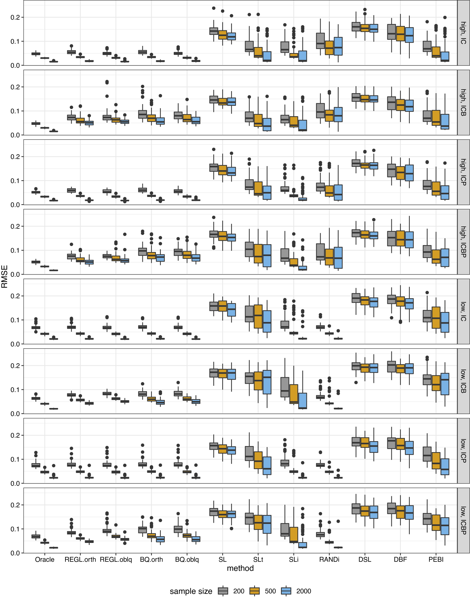
Figure 1 Boxplot of the estimation error for loading matrix under orthogonal bi-factor models.
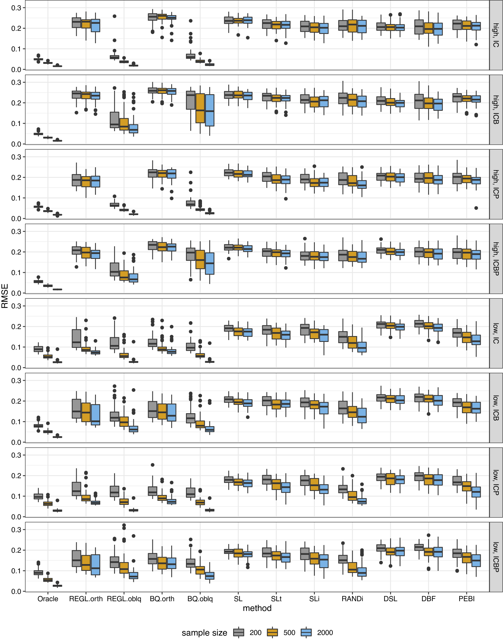
Figure 2 Boxplot of the estimation error for loading matrix under semi-oblique bi-factor models.
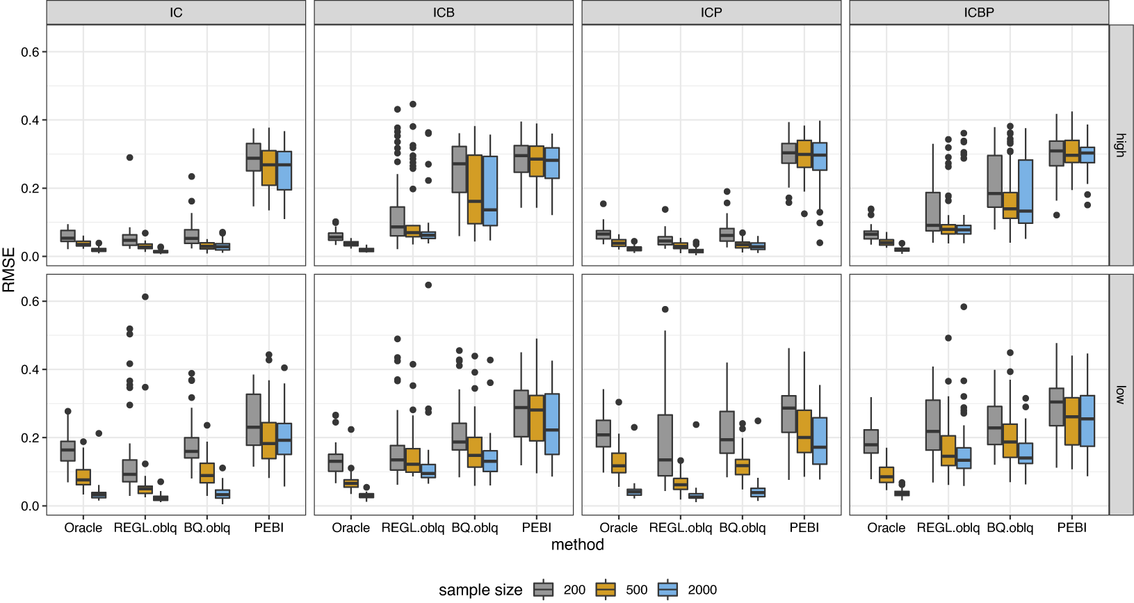
Figure 3 Boxplot of the estimation error for factor correlation matrix under semi-oblique bi-factor models.
Under the orthogonal bi-factor models (Figure 1), our methods and the Bi-Quartimin methods perform best, but our methods are slightly better at recovering the ICB and ICBP structures. Since the orthogonal model is a special case of the oblique model, the oblique versions of these two methods have almost the same performance as their orthogonal counterparts. The SLi method has comparable results to the best ones. We contend that the success of SLi should attribute to the iterating steps. To illustrate this, we replace the SL initialization in the SLi procedure with a random bi-factor loading initialization, and the resultant RANDi method remains successful. Note also the similarity between its iterative spirit and the PAM algorithm. All the other SL-based methods fail to recover the loading matrix.
As for the oblique bi-factor models (Figure 2), our proposed oblique rotation method and the oblique Bi-Quartimin method are the only successful methods, while the oblique PEBI method and all other orthogonal methods fail to provide reasonable estimates. Compared to the Bi-Quartimin method, our method again has an advantage in recovering the ICB and ICBP structures, indicating its robustness. This superiority is more evident when the group loadings take high values. Moreover, our method provides better estimation of the factor correlation matrix than the Bi-Quartimin method, as shown in Figure 3. The accuracy of factor correlation estimation is measured by
 $$\begin{align*}\mathrm{RMSE}(\Phi, \widehat{\Phi}) = \frac{1}{\sqrt{k^2}}\| \Phi - \widehat{\Phi} \|_{\mathrm{F}}. \end{align*}$$
Interestingly, our method can even outperform the oracle method when the underlying model is strictly a bi-factor model. This is because the oracle method minimizes $\|A(T')^{-1} - \Lambda \|_{\mathrm {F}}$
which emphasizes the discrepancy of the loading matrix, and the estimated rotation does not necessarily produce an optimal factor correlation matrix. In contrast, our method minimizes
$\|A(T')^{-1} - \Lambda \|_{\mathrm {F}}$
which emphasizes the discrepancy of the loading matrix, and the estimated rotation does not necessarily produce an optimal factor correlation matrix. In contrast, our method minimizes $\| A - ST'\|_{\mathrm {F}}$
which is compatible with the discrepancy of the covariance matrix, resulting in a rotation that balances the estimation of the loading matrix and the factor correlation matrix. Hence, our method can better estimate the factor correlation matrix even though it does not use the true loading matrix
$\| A - ST'\|_{\mathrm {F}}$
which is compatible with the discrepancy of the covariance matrix, resulting in a rotation that balances the estimation of the loading matrix and the factor correlation matrix. Hence, our method can better estimate the factor correlation matrix even though it does not use the true loading matrix $\Lambda $
. A detailed comparison of the two formulations in estimating the loading matrix and the factor correlation matrix is given in Appendix A.7.
$\Lambda $
. A detailed comparison of the two formulations in estimating the loading matrix and the factor correlation matrix is given in Appendix A.7.
5 Real data examples
5.1 Holzinger’s fourteen tests data
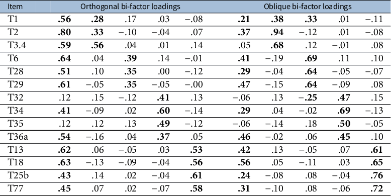
We now apply the proposed exploratory bi-factor analysis approach to Holzinger’s fourteen tests data. This data were used by Holzinger and Swineford (Reference Holzinger and Swineford1937) to illustrate bi-factor analysis. The correlation matrix was provided in Holzinger and Swineford (Reference Holzinger and Swineford1937), and their preliminary analysis divided the fourteen tests into four groups to reflect spatial, mental speed, motor speed, and verbal factors (see Table IV in Holzinger & Swineford, Reference Holzinger and Swineford1937). This bi-factor structure is consistently recovered by our orthogonal and oblique bi-factor analyses, as shown in Table 2, except that the oblique bi-factor model has two crossing loadings. The estimated factor correlation matrix in the oblique model is
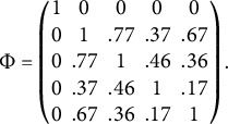 $$\begin{align*}\Phi = \begin{pmatrix} 1 & 0 & 0 & 0 & 0 \\ 0 & 1 & .77 & .37 & .67 \\ 0 & .77 & 1 & .46 & .36 \\ 0 & .37 & .46 & 1 & .17 \\ 0 & .67 & .36 & .17 & 1 \end{pmatrix}. \end{align*}$$
Since both orthogonal and oblique bi-factor analyses recover the desired structure, determining which model is more appropriate may depend on domain knowledge.
Table 2 Exploratory bi-factor rotation results of the proposed methods applied to the fourteen tests data (loadings $\geq .20$
in absolute value are bolded)
$\geq .20$
in absolute value are bolded)
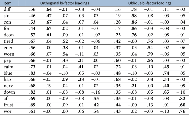
5.2 Quality of life data
When applied to another data set, our methods demonstrate the necessity of oblique bi-factor analysis. Chen et al. (Reference Chen, West and Sousa2006) have applied a confirmatory bi-factor analysis to a Quality of Life data set. This data set contained $403$
observations for
$403$
observations for $17$
items answered on a
$17$
items answered on a $5$
-point Likert scale from
$5$
-point Likert scale from $1$
(all of the time) to
$1$
(all of the time) to $5$
(never), with high scores on the scale indicating a high quality of life. These items were hypothesized to reflect a common general factor (Quality of Life) and four group factors (Cognition, Vitality, Mental Health, and Disease Worry). We apply both the proposed orthogonal and oblique exploratory bi-factor analyses to this data set, with results shown in Table 3. In the orthogonal bi-factor case, not all loadings on the group factor are significant for the third hypothesized cluster (Mental Health), consistent with the published studies (Abad et al., Reference Abad, Garcia-Garzon, Garrido and Barrada2017; Chen et al., Reference Chen, West and Sousa2006; Jennrich & Bentler, Reference Jennrich and Bentler2011). Additionally, we identify a possible cross-loading for the “pep” item, which is also reported by Abad et al. (Reference Abad, Garcia-Garzon, Garrido and Barrada2017). The results become promising in the oblique case, where our method produces a bi-factor structure consistent with the hypothesized structure, except for a potential cross-loading for the “nerv” item. The estimated factor correlation matrix is
$5$
(never), with high scores on the scale indicating a high quality of life. These items were hypothesized to reflect a common general factor (Quality of Life) and four group factors (Cognition, Vitality, Mental Health, and Disease Worry). We apply both the proposed orthogonal and oblique exploratory bi-factor analyses to this data set, with results shown in Table 3. In the orthogonal bi-factor case, not all loadings on the group factor are significant for the third hypothesized cluster (Mental Health), consistent with the published studies (Abad et al., Reference Abad, Garcia-Garzon, Garrido and Barrada2017; Chen et al., Reference Chen, West and Sousa2006; Jennrich & Bentler, Reference Jennrich and Bentler2011). Additionally, we identify a possible cross-loading for the “pep” item, which is also reported by Abad et al. (Reference Abad, Garcia-Garzon, Garrido and Barrada2017). The results become promising in the oblique case, where our method produces a bi-factor structure consistent with the hypothesized structure, except for a potential cross-loading for the “nerv” item. The estimated factor correlation matrix is
 $$\begin{align*}\Phi = \begin{pmatrix} 1 & 0 & 0 & 0 & 0 \\ 0 & 1 & .51 & .65 & .45 \\ 0 & .51 & 1 & .64 & .51 \\ 0 & .65 & .64 & 1 & .65 \\ 0 & .45 & .51 & .65 & 1 \end{pmatrix}, \end{align*}$$
and the group factors have moderate correlations. This might explain the failure of the orthogonal bi-factor models to recover the hypothesized structure.
Table 3 Exploratory bi-factor rotation results of the proposed methods applied to the quality of life data (loadings $\geq .20$
in absolute value are bolded)
$\geq .20$
in absolute value are bolded)
6 Discussion
6.1 Relation to other methods
The rotation to simple structure has been a classic problem in factor analysis, and a number of methods have been proposed in the literature. Although we develop the solution from a different perspective, it is mathematically related to some existing methods. We discuss the connection to Jennrich’s (Reference Jennrich2004) component loss function (CLF) method and Kiers’s (Reference Kiers1994) simplimax method.
Jennrich (Reference Jennrich2004) has investigated a class of rotation criteria based on the CLF including the family of right constant CLF, to which we now demonstrate our method is equivalent. Let $\Lambda = A T$
be the rotated loading matrix with entries
$\Lambda = A T$
be the rotated loading matrix with entries $\lambda _{ir}$
. The CLF method finds the rotation T that minimizes the component loss criterion
$\lambda _{ir}$
. The CLF method finds the rotation T that minimizes the component loss criterion $Q(\Lambda )$
, defined as
$Q(\Lambda )$
, defined as
 $$\begin{align*}Q(\Lambda) = \sum_i \sum_r h(\lambda_{ir}^2) \end{align*}$$
with some component loss function $h(\cdot )$
. One particular CLF is the right constant function
$h(\cdot )$
. One particular CLF is the right constant function
 $$\begin{align*}h(\lambda^2) = \begin{cases} (\lambda / b)^2, \, &\mbox{if } |\lambda | \leq b, \\ 1, \, &\mbox{if } |\lambda |> b. \end{cases} \end{align*}$$
The component loss criterion with this right constant function is equivalent to (2.1) for $\rho = b^2$
. To see this, we rewrite (2.1) as a partial minimization problem
$\rho = b^2$
. To see this, we rewrite (2.1) as a partial minimization problem
 $$ \begin{align} \min_T \big\{ \min_S \big( \|AT - S\|_{\mathrm{F}}^2 + \rho \|S\|_0 \big) \big\}. \end{align} $$
The inner minimization problem over S has an explicit solution $S = S(T) := \mathcal {H}(AT, \sqrt {\rho })$
. Thus, if we let
$S = S(T) := \mathcal {H}(AT, \sqrt {\rho })$
. Thus, if we let $\Lambda = AT$
, (6.1) becomes
$\Lambda = AT$
, (6.1) becomes
 $$ \begin{align*} \min_T ~ &\|AT - S(T)\|_{\mathrm{F}}^2 + \rho \|S(T)\|_0 \cr &= \min_T ~ \sum_i \sum_r \big\{\lambda_{ir}^2 I(\lambda_{ir}^2 \leq {\rho}) + \rho I(\lambda_{ir}^2> {\rho}) \big\}, \end{align*} $$
which is exactly $b^2 Q(\Lambda )$
with the right constant CLF and
$b^2 Q(\Lambda )$
with the right constant CLF and $\rho = b^2$
. This equivalence has several consequences. First, the desirable properties of the right constant CLF provided by Jennrich (Reference Jennrich2004) directly apply to our method, such as the ability to recover perfect simple structure or Thurstone’s simple structure whenever they exist. Second, it suggests choosing the tuning parameter
$\rho = b^2$
. This equivalence has several consequences. First, the desirable properties of the right constant CLF provided by Jennrich (Reference Jennrich2004) directly apply to our method, such as the ability to recover perfect simple structure or Thurstone’s simple structure whenever they exist. Second, it suggests choosing the tuning parameter $\rho $
as the square of the threshold b, such as
$\rho $
as the square of the threshold b, such as $\rho = 0.3^2$
. Finally, our method provides a natural justification and interpretation for the right constant CLF, and we also offer a simple and convergent algorithm for the equivalent methods.
$\rho = 0.3^2$
. Finally, our method provides a natural justification and interpretation for the right constant CLF, and we also offer a simple and convergent algorithm for the equivalent methods.
Another related method is the simplimax rotation (Kiers, Reference Kiers1994). Although the simplimax method is proposed for oblique rotation, the idea can be analogously applied to the orthogonal rotation. Given a number m, the simplimax maximizes the simplicity by minimizing the sum of m smallest squared entries of the rotated loading matrix. It is derived from the formulation:
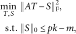 $$ \begin{align} \begin{aligned} \min_{T,S} ~&\|AT - S\|_{\mathrm{F}}^2, \cr \mathrm{s.t.} ~ &\|S\|_0 \leq pk-m, \end{aligned} \end{align} $$
where T is either an orthogonal or an oblique rotation matrix. Thus, the simplimax can be viewed as a constrained version of (2.1), while (2.1) is a penalized version. The PAM algorithm is still applicable to the constrained problem (6.2), in which (2.3) is replaced by a truncation operation that sets the m smallest (in absolute value) entries of ${(A T_{t+1} + \eta _t S_t)}/{(1+\eta _t)}$
to zero. The constrained version (6.2) is appropriate when the number of zero loadings is pre-specified, while the penalized version (2.1) is appropriate when the threshold for small loadings is given, which is typically the case.
${(A T_{t+1} + \eta _t S_t)}/{(1+\eta _t)}$
to zero. The constrained version (6.2) is appropriate when the number of zero loadings is pre-specified, while the penalized version (2.1) is appropriate when the threshold for small loadings is given, which is typically the case.
In developing the approach of exploratory bi-factor analysis, Jennrich and Bentler (Reference Jennrich and Bentler2011, Reference Jennrich and Bentler2012) proposed constructing the rotation criterion as an index that measures the departure of a loading matrix from a bi-factor structure. If such departure is measured by the Frobenius distance to the set of bi-factor loading matrices, one naturally derives our formulation (2.4). Formulation (3.6) measures a distance not directly under the loading matrix scale but under the covariance matrix scale. This scale has the benefit of balancing the estimation accuracy for the loading matrix and the factor correlation matrix, hence the better performance shown in Figure 3.
6.2 Bridging simple structure rotation and penalized estimation
Penalized estimation is a popular technique in statistics and machine learning for incorporating prior knowledge about parameters. When the parameters are assumed to be sparse, sparsity-promoting penalties such as the Lasso (Tibshirani, Reference Tibshirani1996) are incorporated into the loss functions (e.g., the likelihood function) to produce sparse estimates. This technique has been introduced to the EFA for the estimation of sparse loadings and has been suggested as an alternative to the factor rotation procedure because it produces sparser loadings (Hirose & Yamamoto, Reference Hirose and Yamamoto2015; Scharf & Nestler, Reference Scharf and Nestler2019). We now show via our framework that the factor rotation procedure and the penalized estimation are two sides of the same coin. Their relation is summarized in Table 4. In the REGL formulation (2.1), the optimal value for S given a fixed T is $\mathcal {H}(AT, \sqrt {\rho })$
, and the optimal value for T given a fixed S is
$\mathcal {H}(AT, \sqrt {\rho })$
, and the optimal value for T given a fixed S is $\mathcal {P}_{\mathrm {orth}} (A' S) = \mathrm {arg} \min _{\{T: T'T=\mathbf {I}_k\}} \|AT-S\|_{\mathrm {F}}$
. Thus, the penalized estimate S is a truncated matrix of the rotated loading
$\mathcal {P}_{\mathrm {orth}} (A' S) = \mathrm {arg} \min _{\{T: T'T=\mathbf {I}_k\}} \|AT-S\|_{\mathrm {F}}$
. Thus, the penalized estimate S is a truncated matrix of the rotated loading $AT$
, and the rotated loading
$AT$
, and the rotated loading $AT$
is an untruncated version of S. The difference between the rotation procedure and penalized estimation is merely a matter of choosing the output between
$AT$
is an untruncated version of S. The difference between the rotation procedure and penalized estimation is merely a matter of choosing the output between $AT$
and S.
$AT$
and S.
Table 4 Classification of estimation procedures
While one may argue that our sparse estimates S in (2.1) and (3.2) are not exactly the penalized likelihood estimations discussed in the literature, the difference is peripheral. The classic penalized estimation minimizes a loss function (e.g., the likelihood function or the squared loss) $d(\widehat {\Sigma }, S \Phi S' + \Psi ^2)$
, which represents the discrepancy between the sample covariance matrix
$d(\widehat {\Sigma }, S \Phi S' + \Psi ^2)$
, which represents the discrepancy between the sample covariance matrix $\widehat {\Sigma }$
and the model covariance matrix
$\widehat {\Sigma }$
and the model covariance matrix $S \Phi S' + \Psi ^2$
, along with a penalty term for S. In contrast, we minimize
$S \Phi S' + \Psi ^2$
, along with a penalty term for S. In contrast, we minimize $\| {A} - S T' \|_{\mathrm {F}}^2$
plus a penalty term. The loss function
$\| {A} - S T' \|_{\mathrm {F}}^2$
plus a penalty term. The loss function $d(\widehat {\Sigma }, S \Phi S' + \Psi ^2)$
can be quadratically approximated (up to constant scaling and shifting) by
$d(\widehat {\Sigma }, S \Phi S' + \Psi ^2)$
can be quadratically approximated (up to constant scaling and shifting) by $\| {A} {A}' - S \Phi S' \|_{\mathrm {F}}^2$
, as
$\| {A} {A}' - S \Phi S' \|_{\mathrm {F}}^2$
, as $AA' + \widehat {\Psi }^2$
is the minimizer of the loss function. Taking the “square root” of the matrices
$AA' + \widehat {\Psi }^2$
is the minimizer of the loss function. Taking the “square root” of the matrices $AA'$
and
$AA'$
and $S \Phi S' = S T'T S'$
, we can further approximate
$S \Phi S' = S T'T S'$
, we can further approximate $\| {A} {A}' - S \Phi S' \|_{\mathrm {F}}^2$
by
$\| {A} {A}' - S \Phi S' \|_{\mathrm {F}}^2$
by $\| {A} - S T' \|_{\mathrm {F}}^2$
. Therefore, our formulas (2.1) and (3.2) are approximated penalized loss functions, and our sparse estimates S are approximate solutions to the standard penalized estimation. Ideally, it would be best to solve the penalized loss function directly because the initial loading matrix A is only an intermediate estimator. We frame the problem within the rotation paradigm partly because factor rotation procedures have historically been central to the EFA and partly because the rotation of a given matrix presents an algebraic problem of independent interest. Moreover, employing a penalized loss function introduces challenges in solving the optimization problem, as our algorithm is neither practical nor necessarily convergent when applied to it. The exploration of efficient algorithms for minimizing the penalized loss function in factor analysis remains a topic for future research.
$\| {A} - S T' \|_{\mathrm {F}}^2$
. Therefore, our formulas (2.1) and (3.2) are approximated penalized loss functions, and our sparse estimates S are approximate solutions to the standard penalized estimation. Ideally, it would be best to solve the penalized loss function directly because the initial loading matrix A is only an intermediate estimator. We frame the problem within the rotation paradigm partly because factor rotation procedures have historically been central to the EFA and partly because the rotation of a given matrix presents an algebraic problem of independent interest. Moreover, employing a penalized loss function introduces challenges in solving the optimization problem, as our algorithm is neither practical nor necessarily convergent when applied to it. The exploration of efficient algorithms for minimizing the penalized loss function in factor analysis remains a topic for future research.
We can further draw a connection with the confirmatory factor analysis (CFA). In the CFA, the likelihood function (or a loss function in general) is minimized under the restriction where certain loading entries are pre-specified with fixed values or subject to equality constraints. This approach constitutes constrained estimation. Similar to the penalized formulation, our REGL framework provides a mathematical correspondence between the rotation procedure and the constrained estimation. The constrained estimates produced by our framework are again approximate solutions for CFA estimation by substituting the standard loss function with $\| {A} - S T' \|_{\mathrm {F}}^2$
. Although the exploratory and confirmatory factor analyses are usually considered distinct disciplines with different objectives, our framework reveals a mathematical connection between their estimates.
$\| {A} - S T' \|_{\mathrm {F}}^2$
. Although the exploratory and confirmatory factor analyses are usually considered distinct disciplines with different objectives, our framework reveals a mathematical connection between their estimates.
7 Conclusion
We have proposed a general framework to solve the rotation problem in factor analysis. The problem is formulated as either a penalized or a constrained optimization, depending on the type of rotation purpose. This regularized formulation can incorporate any desired assumptions about the factor structure, and the optimization process finds the optimal rotation based on these assumptions. The optimization problem is solved using simple and convergent algorithms. This framework is applicable to both orthogonal and oblique rotations. We illustrate the penalized and constrained formulations using examples of simple structure rotation and bi-factor rotation, respectively.
Simulation studies show that, for exploratory bi-factor analysis, our method performs better than most other methods under many conditions, and mostly equally well as Bi-Quartimin, except in the conditions ICB and ICBP, where it performs better than Bi-Quartimin. When applied to real data sets, our method uncovers bi-factor structures that are consistent with the hypothesized theory. Our framework also provides insight into the mathematical relationship among exploratory factor rotation, penalized estimation, and confirmatory factor analysis.
Finally, we want to point out that we are essentially providing a numerical iterative approach to an algebraic problem: given a matrix A, how to find its approximate factorization $ST'$
where S and T satisfy certain structures or properties. This matrix factorization framework has potential applications beyond factor analysis and could be valuable in other fields. For example, in dictionary learning (Rubinstein et al., Reference Rubinstein, Bruckstein and Elad2010; Zhai et al., Reference Zhai, Yang, Liao, Wright and Ma2020), the problem of sparse representation modeling can be approached in a manner similar to (2.1) for orthogonal dictionaries or (3.2) for general dictionaries. The potential connections and extensions of our algebraic framework to related problems may be explored in future work. A reviewer raised a question regarding the performance of formulation (3.1) for the oblique rotation problem. We have not yet identified a convergent algorithm for solving (3.1), although some preliminary findings are presented in Appendix A.7. A comprehensive and systematic study of (3.1) represents another promising direction for future research.
$ST'$
where S and T satisfy certain structures or properties. This matrix factorization framework has potential applications beyond factor analysis and could be valuable in other fields. For example, in dictionary learning (Rubinstein et al., Reference Rubinstein, Bruckstein and Elad2010; Zhai et al., Reference Zhai, Yang, Liao, Wright and Ma2020), the problem of sparse representation modeling can be approached in a manner similar to (2.1) for orthogonal dictionaries or (3.2) for general dictionaries. The potential connections and extensions of our algebraic framework to related problems may be explored in future work. A reviewer raised a question regarding the performance of formulation (3.1) for the oblique rotation problem. We have not yet identified a convergent algorithm for solving (3.1), although some preliminary findings are presented in Appendix A.7. A comprehensive and systematic study of (3.1) represents another promising direction for future research.
Supplementary material
The supplementary material for this article can be found at https://doi.org/10.1017/psy.2025.1.
Acknowledgments
The authors wish to thank Dan Bolt for his helpful feedback on drafts of this article. The authors also kindly thank the editor, the associate editor, and two anonymous referees for their insightful comments and suggestions that greatly improve this article.
Funding statement
Q.L. is partially supported by the National Nature Science Foundation of China (Grant Nos. 12325110 and 12288201) and the CAS Project for Young Scientists in Basic Research (YSBR-034).
Competing interests
The authors have no competing interests to declare that are relevant to the content of this article.
1 Appendix
A.1 Derivation of Algorithm 1
For the problem (2.1), the PAM algorithm (Attouch et al., Reference Attouch, Bolte, Redont and Soubeyran2010) reads
Step (A.1) is a proximal version of Procrustes problem, and can be converted to a standard one:
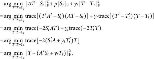 $$\begin{align*}\begin{aligned} &\mathrel{\phantom{=}} \mathrm{arg} \min_{T'T = \mathbf{I}_k} \|AT - S_t\|_{\mathrm{F}}^2 + \rho \|S_t\|_0 + \gamma_t \| T - T_t \|_{\mathrm{F}}^2 \\ &= \mathrm{arg} \min_{T'T = \mathbf{I}_k} \mathrm{trace} [ (T'A' - S^{\prime}_t)(AT - S_t)] + \gamma_t \mathrm{trace}[(T'-T^{\prime}_t)(T-T_t)] \\ &= \mathrm{arg} \min_{T'T = \mathbf{I}_k} \mathrm{trace}(-2S^{\prime}_tAT) + \gamma_t \mathrm{trace} (-2 T^{\prime}_t T) \\ &= \mathrm{arg} \min_{T'T = \mathbf{I}_k} \mathrm{trace} [-2 (S^{\prime}_tA + \gamma_t T^{\prime}_t)T] \\ &= \mathrm{arg} \min_{T'T = \mathbf{I}_k} \| T - (A'S_t + \gamma_t T_t) \|_{\mathrm{F}}^2. \end{aligned} \end{align*}$$
Thus $T_{t+1} = \mathcal {P}_{\mathrm {orth}} (A'S_t + \gamma _t T_t)$
. Step (A.2) can be rearranged to
$T_{t+1} = \mathcal {P}_{\mathrm {orth}} (A'S_t + \gamma _t T_t)$
. Step (A.2) can be rearranged to
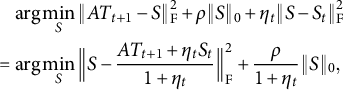 $$\begin{align*}\begin{aligned} &\mathrel{\phantom{=}} \mathrm{arg} \min_S \|AT_{t+1} - S\|_{\mathrm{F}}^2 + \rho \|S\|_0 + \eta_t \| S - S_t \|_{\mathrm{F}}^2 \\ &= \mathrm{arg} \min_S \Big\| S - \frac{A T_{t+1} + \eta_t S_t}{1+\eta_t} \Big\|_{\mathrm{F}}^2 + \frac{\rho}{1+\eta_t} \| S \|_0, \end{aligned} \end{align*}$$
which can be optimized entry-wisely. In general, function $(x-t)^2 + \kappa \|x\|_0$
is minimized at
$(x-t)^2 + \kappa \|x\|_0$
is minimized at $x=0$
if
$x=0$
if $|t| < \sqrt {\kappa }$
and at
$|t| < \sqrt {\kappa }$
and at $x=t$
otherwise, that is, the minimizer is
$x=t$
otherwise, that is, the minimizer is $x = \mathcal {H}(t, \sqrt {\kappa })$
. Hence,
$x = \mathcal {H}(t, \sqrt {\kappa })$
. Hence,
 $$\begin{align*}S_{t+1} = \mathcal{H} \Big( \frac{A T_{t+1} + \eta_t S_t}{1+\eta_t}, \sqrt{{\rho}/{(1+\eta_t)}} \Big). \end{align*}$$
A.2 Proof of Proposition 1
This convergence result is a direct application of Theorem 3.2 in Attouch et al. (Reference Attouch, Bolte, Redont and Soubeyran2010). In particular, Theorem 3.2 of Attouch et al. (Reference Attouch, Bolte, Redont and Soubeyran2010) requires that the objective function has the Kurdyka–Łojasiewicz property and that its smooth part has a Lipschitz continuous gradient. A function $f(x)$
is called Lipschitz continuous if there exists a constant
$f(x)$
is called Lipschitz continuous if there exists a constant $L \geq 0$
such that
$L \geq 0$
such that $\|f(x) - f(y)\| \leq L \|x - y \|$
for all x and y. The constant L is called the Lipschitz modulus. The function
$\|f(x) - f(y)\| \leq L \|x - y \|$
for all x and y. The constant L is called the Lipschitz modulus. The function $\|AT-S\|_{\mathrm {F}}^2$
in (2.1) is a quadratic function of T and S, so it is continuously differentiable and has a Lipschitz continuous gradient on bounded subsets. Theorem 3 in Bolte et al. (Reference Bolte, Sabach and Teboulle2014) shows that semi-algebraic functions must have the Kurdyka–Łojasiewicz property (both definitions can be found in Attouch et al., Reference Attouch, Bolte, Redont and Soubeyran2010 or Bolte et al., Reference Bolte, Sabach and Teboulle2014). Semi-algebraic functions are ubiquitous. In particular, polynomial functions, the Stiefel manifold (i.e., the set of orthogonal matrices), and
$\|AT-S\|_{\mathrm {F}}^2$
in (2.1) is a quadratic function of T and S, so it is continuously differentiable and has a Lipschitz continuous gradient on bounded subsets. Theorem 3 in Bolte et al. (Reference Bolte, Sabach and Teboulle2014) shows that semi-algebraic functions must have the Kurdyka–Łojasiewicz property (both definitions can be found in Attouch et al., Reference Attouch, Bolte, Redont and Soubeyran2010 or Bolte et al., Reference Bolte, Sabach and Teboulle2014). Semi-algebraic functions are ubiquitous. In particular, polynomial functions, the Stiefel manifold (i.e., the set of orthogonal matrices), and $\| \cdot \|_0$
are all semi-algebraic (see the Appendix in Bolte et al., Reference Bolte, Sabach and Teboulle2014). Hence, the objective function (2.1) has the Kurdyka–Łojasiewicz property.
$\| \cdot \|_0$
are all semi-algebraic (see the Appendix in Bolte et al., Reference Bolte, Sabach and Teboulle2014). Hence, the objective function (2.1) has the Kurdyka–Łojasiewicz property.
Theorem 3.2 in Attouch et al. (Reference Attouch, Bolte, Redont and Soubeyran2010) implies that any bounded sequence converges to a stationary point. We now show that our sequence is bounded. The orthogonal matrix $T_t$
is bounded. The iteration (2.3) implies that
$T_t$
is bounded. The iteration (2.3) implies that
 $$\begin{align*}\begin{aligned} \|S_{t+1}\|_{\mathrm{F}} &= \Big\| \mathcal{H} \Big( \frac{A T_{t+1} + \eta_t S_t}{1+\eta_t}, \sqrt{{\rho}/{(1+\eta_t)}} \Big)\Big\|_{\mathrm{F}} \cr &\leq \Big\| \frac{A T_{t+1} + \eta_t S_t}{1+\eta_t} \Big\|_{\mathrm{F}} \cr &\leq \Big\|\frac{A T_{t+1}}{1+\eta_t}\Big\|_{\mathrm{F}} + \Big \|\frac{\eta_tS_t}{1+\eta_t}\Big\|_{\mathrm{F}} \\ &= \frac{1}{1+\eta_t}\|A\|_{\mathrm{F}} + \frac{\eta_t}{1+\eta_t} \|S_t\|_{\mathrm{F}} \\ &\leq \frac{1}{1+\eta_t}\max \{\|A\|_{\mathrm{F}}, \|S_t\|_{\mathrm{F}}\} + \frac{\eta_t}{1+\eta_t}\max \{\|A\|_{\mathrm{F}}, \|S_t\|_{\mathrm{F}}\} \\ &= \max \{\|A\|_{\mathrm{F}}, \|S_t\|_{\mathrm{F}}\}. \end{aligned} \end{align*}$$
This is valid for any t. Therefore,
 $$\begin{align*}\begin{aligned} \|S_{t+1}\|_{\mathrm{F}} &\leq \max \{\|A\|_{\mathrm{F}}, \|S_t\|_{\mathrm{F}}\} \cr &\leq \max \big\{\|A\|_{\mathrm{F}}, \max \{\|A\|_{\mathrm{F}}, \|S_{t-1}\|_{\mathrm{F}}\}\big\} \\ &= \max \{\|A\|_{\mathrm{F}}, \|S_{t-1}\|_{\mathrm{F}}\} \\ &\leq \cdots \\ &\leq \max \{\|A\|_{\mathrm{F}}, \|S_0\|_{\mathrm{F}}\}. \end{aligned} \end{align*}$$
Hence our sequence $(T_t, S_t)$
is bounded and thus converges to a stationary point.
$(T_t, S_t)$
is bounded and thus converges to a stationary point.
A.3 Projection onto bi-factor loadings
Algorithms 2 and 4 involve projecting a matrix onto the set of bi-factor loading matrices $\mathcal {P}_{\mathrm {bi}}(X) = \mathrm {arg} \min _{S \in \mathcal {S}_{\mathrm {bi}}} \|S - X \|_{\mathrm {F}}$
. To find this projection, one needs to identify which column of S corresponds to the general factor. Suppose that the rth column of S represents the general factor loadings; then this column is free and should be equal to the rth column of X in order to minimize the Frobenius distance. After that, simple algebra shows that the group factor loadings in S should be identical (in both value and location) to the largest (in absolute value) entry in each row of the remaining X sub-matrix. By letting every column be a potential general factor loading, we obtain k candidates for the bi-factor loading matrices. The projection will be the one with the largest Frobenius norm, because in this case
$\mathcal {P}_{\mathrm {bi}}(X) = \mathrm {arg} \min _{S \in \mathcal {S}_{\mathrm {bi}}} \|S - X \|_{\mathrm {F}}$
. To find this projection, one needs to identify which column of S corresponds to the general factor. Suppose that the rth column of S represents the general factor loadings; then this column is free and should be equal to the rth column of X in order to minimize the Frobenius distance. After that, simple algebra shows that the group factor loadings in S should be identical (in both value and location) to the largest (in absolute value) entry in each row of the remaining X sub-matrix. By letting every column be a potential general factor loading, we obtain k candidates for the bi-factor loading matrices. The projection will be the one with the largest Frobenius norm, because in this case $\|S - X\|_{\mathrm {F}}^2 = \|X\|_{\mathrm {F}}^2 - \|S\|_{\mathrm {F}}^2$
for those candidate matrices S.
$\|S - X\|_{\mathrm {F}}^2 = \|X\|_{\mathrm {F}}^2 - \|S\|_{\mathrm {F}}^2$
for those candidate matrices S.
A.4 Derivation of Algorithm 3
For the minimization of $H(T,S) + f(T) + g(S)$
, the PALM algorithm (Bolte et al., Reference Bolte, Sabach and Teboulle2014) reads
$H(T,S) + f(T) + g(S)$
, the PALM algorithm (Bolte et al., Reference Bolte, Sabach and Teboulle2014) reads
In our case (3.2), $H(T,S) = \|A - ST'\|_{\mathrm {F}}^2$
,
$H(T,S) = \|A - ST'\|_{\mathrm {F}}^2$
, $g(S) = \rho \|S\|_0$
, and
$g(S) = \rho \|S\|_0$
, and $f(T)$
is the indicator function for the constraint
$f(T)$
is the indicator function for the constraint $\mathrm {diag} (T'T) = \mathbf {I}_k$
, i.e.,
$\mathrm {diag} (T'T) = \mathbf {I}_k$
, i.e., $f(T) = 0$
if T belongs to the constraint, and
$f(T) = 0$
if T belongs to the constraint, and $f(T)= + \infty $
otherwise. We have
$f(T)= + \infty $
otherwise. We have
 $$\begin{align*}\nabla_T H(T,S) = -2(A' - TS')S, \mbox{ and } \nabla_S H(T,S) = -2(A-ST')T. \end{align*}$$
For these functions,
 $$\begin{align*}\| \nabla_T H(T_1,S) - \nabla_T H(T_2,S) \|_{\mathrm{F}} = \| 2(T_1 - T_2) S'S \|_{\mathrm{F}} \leq 2 \|T_1 - T_2 \|_{\mathrm{F}} \| S'S \|_{\mathrm{F}} \end{align*}$$
and
 $$\begin{align*}\| \nabla_S H(T,S_1) - \nabla_S H(T,S_2) \|_{\mathrm{F}} = \| 2(S_1 - S_2) T'T \|_{\mathrm{F}} \leq 2 \|S_1 - S_2 \|_{\mathrm{F}} \| T'T \|_{\mathrm{F}}, \end{align*}$$
so they are Lipschitz continuous with moduli $L_1(S) = 2 \|S'S\|_{\mathrm {F}}$
and
$L_1(S) = 2 \|S'S\|_{\mathrm {F}}$
and $L_2(T) = 2 \|T'T\|_{\mathrm {F}}$
, respectively. The PALM algorithm requires that
$L_2(T) = 2 \|T'T\|_{\mathrm {F}}$
, respectively. The PALM algorithm requires that $c_t = \gamma L_1(S_t)$
and
$c_t = \gamma L_1(S_t)$
and $d_t = \eta L_2(T_{t+1})$
for some
$d_t = \eta L_2(T_{t+1})$
for some $\gamma>1, \eta >1$
. Thus, (A.3) becomes
$\gamma>1, \eta >1$
. Thus, (A.3) becomes
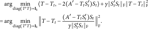 $$\begin{align*}\begin{aligned} &\mathrel{\phantom{=}} \mathrm{arg} \min_{\mathrm{diag}(T'T) = \mathbf{I}_k} \langle T - T_t, -2(A' - T_tS^{\prime}_t)S_t \rangle + \gamma \|S_{t}^{\prime}S_t\|_{\mathrm{F}} \| T - T_t \|_{\mathrm{F}}^2 \\ &= \mathrm{arg} \min_{\mathrm{diag}(T'T) = \mathbf{I}_k} \Big\| T - T_t - \frac{(A' - T_tS^{\prime}_t)S_t}{\gamma \|S^{\prime}_tS_t\|_{\mathrm{F}}} \Big\|_{\mathrm{F}}^2. \end{aligned} \end{align*}$$
Therefore,
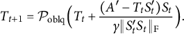 $$\begin{align*}T_{t+1} = \mathcal{P}_{\mathrm{oblq}} \Big(T_t + \frac{(A' - T_tS_{t}^{\prime})S_t}{\gamma \|S_{t}^{\prime} S_t \|_{\mathrm{F}}} \Big). \end{align*}$$
Step (A.4) becomes
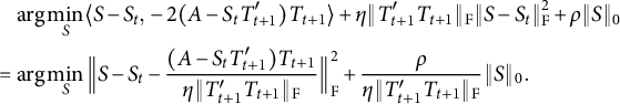 $$\begin{align*}\begin{aligned} &\mathrel{\phantom{=}} \mathrm{arg} \min_{S} \langle S - S_t, -2(A - S_tT^{\prime}_{t+1})T_{t+1} \rangle + \eta \|T^{\prime}_{t+1}T_{t+1}\|_{\mathrm{F}} \| S - S_t \|_{\mathrm{F}}^2 + \rho \|S \|_0 \\ &= \mathrm{arg} \min_{S} \Big\| S - S_t - \frac{(A - S_tT^{\prime}_{t+1})T_{t+1}}{\eta \|T^{\prime}_{t+1}T_{t+1}\|_{\mathrm{F}}} \Big\|_{\mathrm{F}}^2 + \frac{\rho}{\eta \|T^{\prime}_{t+1}T_{t+1}\|_{\mathrm{F}}} \|S\|_0. \end{aligned} \end{align*}$$
Hence
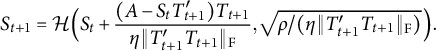 $$\begin{align*}S_{t+1} = \mathcal{H} \Big( S_t + \frac{(A - S_t T_{t+1}^{\prime})T_{t+1}}{\eta \|T_{t+1}^{\prime}T_{t+1}\|_{\mathrm{F}}}, \sqrt{{\rho}/{(\eta \|T_{t+1}^{\prime}T_{t+1}\|_{\mathrm{F}})}} \Big). \end{align*}$$
A.5 Proof of Proposition 2
This convergence result is a direct application of Theorem 1 in Bolte et al. (Reference Bolte, Sabach and Teboulle2014). Specifically, the constraint $\mathrm {diag}(T'T) = \mathbf {I}_k$
is defined by a series of polynomial equations, so it is semi-algebraic by definition. Similar to the proof of Proposition 1, the other terms in (3.2) are also semi-algebraic. Therefore, (3.2) has the Kurdyka–Łojasiewicz property. The Assumptions 1 and 2 required in Bolte et al. (Reference Bolte, Sabach and Teboulle2014) can be easily verified to be true for (3.2). Thus, the bounded iterates
$\mathrm {diag}(T'T) = \mathbf {I}_k$
is defined by a series of polynomial equations, so it is semi-algebraic by definition. Similar to the proof of Proposition 1, the other terms in (3.2) are also semi-algebraic. Therefore, (3.2) has the Kurdyka–Łojasiewicz property. The Assumptions 1 and 2 required in Bolte et al. (Reference Bolte, Sabach and Teboulle2014) can be easily verified to be true for (3.2). Thus, the bounded iterates $(T_t, S_t)$
converge to a stationary point.
$(T_t, S_t)$
converge to a stationary point.
A.6 Simulation on simple structure rotation
This section provides the simulation results of the proposed method and existing methods for recovering simple structure in EFA. The simulation setting is very similar to that of the bi-factor rotation simulation in Section 4. There are a total of $22$
items, and they admit a factor model with a perfect simple structure. There are four latent common factors, and these common factors have nonzero loadings on four, five, six, and seven items, respectively. The nonzero loadings are randomly selected from the intervals
$22$
items, and they admit a factor model with a perfect simple structure. There are four latent common factors, and these common factors have nonzero loadings on four, five, six, and seven items, respectively. The nonzero loadings are randomly selected from the intervals $[0.3,0.6]$
or
$[0.3,0.6]$
or $[0.6, 0.9]$
, and then each entry is randomly assigned a positive or negative sign. The population correlation matrix is generated as
$[0.6, 0.9]$
, and then each entry is randomly assigned a positive or negative sign. The population correlation matrix is generated as
 $$\begin{align*}R = \Lambda \Phi \Lambda' + \Psi^2, \end{align*}$$
where $\Phi $
is the factor correlation matrix and
$\Phi $
is the factor correlation matrix and $\Psi ^2$
is a diagonal matrix of uniqueness, chosen to constrain the diagonal elements of R to one. In the orthogonal model,
$\Psi ^2$
is a diagonal matrix of uniqueness, chosen to constrain the diagonal elements of R to one. In the orthogonal model, $\Phi $
will be an identity matrix. In the oblique model, the correlations among common factors are randomly selected from the interval
$\Phi $
will be an identity matrix. In the oblique model, the correlations among common factors are randomly selected from the interval $[0.2, 0.6]$
. If the generated correlation matrix is not positive definite, we re-generate a new one until it is positive definite. The final step generates the data from a multivariate normal distribution with zero mean and covariance matrix R, with a sample size
$[0.2, 0.6]$
. If the generated correlation matrix is not positive definite, we re-generate a new one until it is positive definite. The final step generates the data from a multivariate normal distribution with zero mean and covariance matrix R, with a sample size $N \in \{200, 500, 2000\}$
. The simulation is replicated
$N \in \{200, 500, 2000\}$
. The simulation is replicated $50$
times for each scenario. The estimation accuracy is evaluated by the RMSE (4.1).
$50$
times for each scenario. The estimation accuracy is evaluated by the RMSE (4.1).
We compare our proposed methods with the conventional rotation methods, namely, the Varimax for orthogonal rotation and the oblimin for oblique rotation. The results are shown in Figures A.1 and A.2. The oracle method rotates the initial loading matrix toward the true loading matrix, so it is optimal in the sense of minimizing the RMSE of loading matrix estimation. Under the orthogonal model, all the methods achieve nearly optimal performance. Under the oblique model, these oblique methods (REGL.oblq and oblimin) are as good as the oracle method. Nonetheless, as shown in Figure A.2, our method has better performance in estimating the factor correlations. Our method exhibits outliers in Figures A.1 and A.2 because it gets trapped in local minima in these cases.
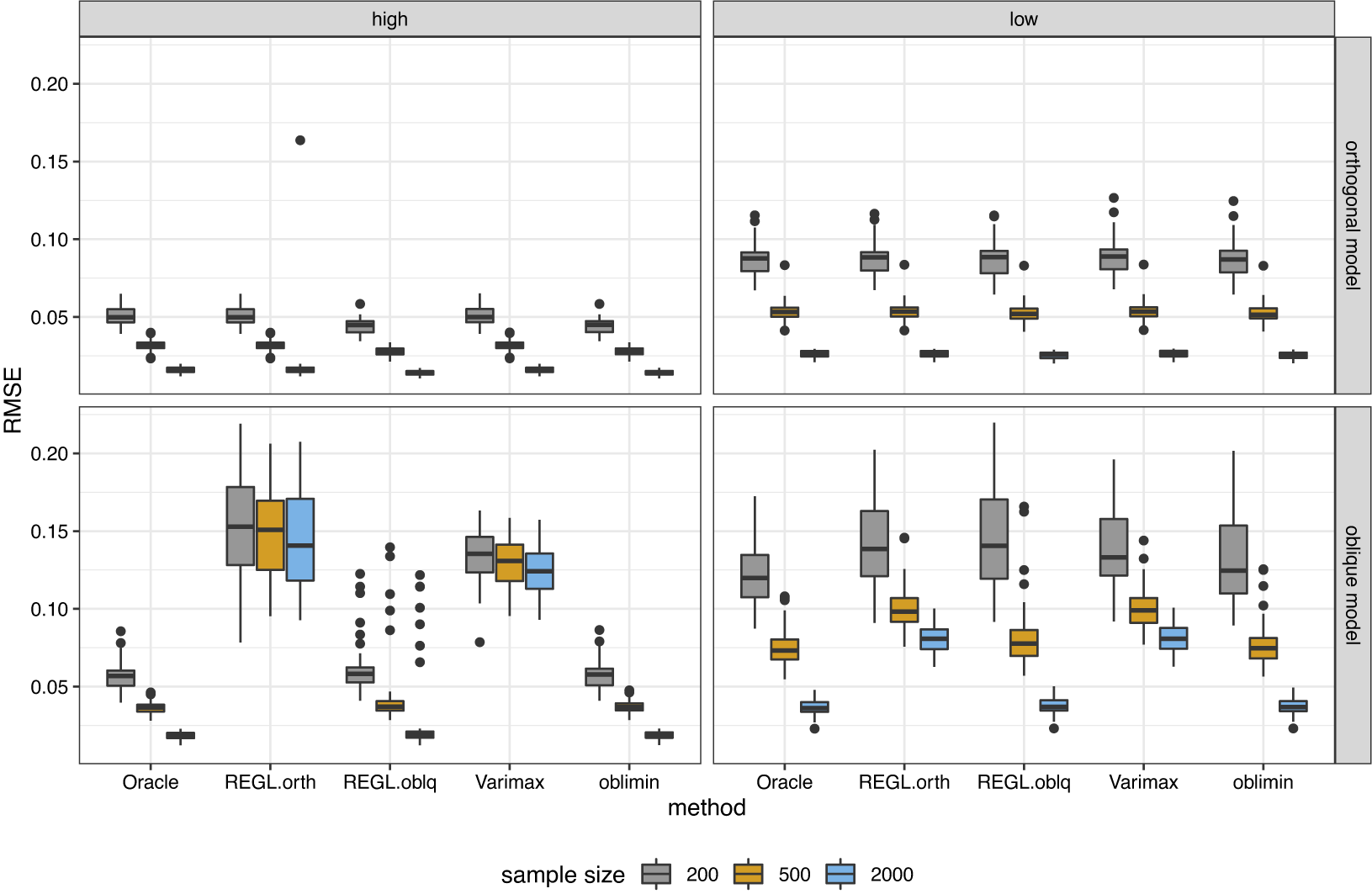
Figure A.1 Boxplot of the estimation error for loading matrix under factor models with perfect simple structure.
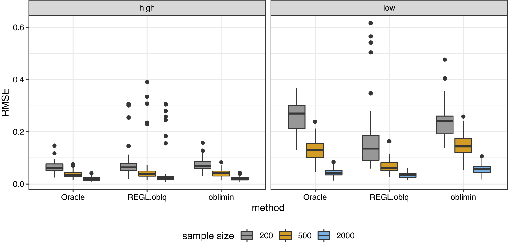
Figure A.2 Boxplot of the estimation error for factor correlation matrix under oblique factor models with perfect simple structure.
A.7 Comparing two formulations of oblique rotation
This section investigates the performance of two different formulations of the oblique rotation problem through simulations. The simulation settings are exactly the same as those in Section 4. The two formulations are
 $$ \begin{align} \begin{aligned} \min_{T,S}&~ \|A (T')^{-1}- S\|_{\mathrm{F}}^2, \cr \mathrm{s.t.} &~ \mathrm{diag}(T'T) = \mathbf{I}_k, \: S \in \mathcal{S}_{\mathrm{bi}} , \end{aligned} \end{align} $$
and
 $$ \begin{align} \begin{aligned} \min_{T,S}&~ \|A - S T'\|_{\mathrm{F}}^2, \cr \mathrm{s.t.} &~ \mathrm{diag}(T'T) = \mathbf{I}_k, \: S \in \mathcal{S}_{\mathrm{bi}}. \end{aligned} \end{align} $$
(A.5) is solved by the alternating minimization algorithm and the updating of T given a fixed S is achieved by Jennrich (Reference Jennrich2002)’s gradient projection algorithm. (A.6) is solved by Algorithm 4. Both solutions are partially orthogonalized to the semi-oblique bi-factor results. The two corresponding oracle methods are
 $$ \begin{align} \begin{aligned} \min_{T}&~ \|A (T')^{-1}- \Lambda\|_{\mathrm{F}}^2, \cr \mathrm{s.t.} &~ \mathrm{diag}(T'T) = \mathbf{I}_k, \end{aligned} \end{align} $$
and
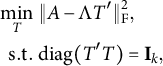 $$ \begin{align} \begin{aligned} \min_{T}&~ \|A - \Lambda T'\|_{\mathrm{F}}^2, \cr \mathrm{s.t.} &~ \mathrm{diag}(T'T) = \mathbf{I}_k, \end{aligned} \end{align} $$
where $\Lambda $
is the true loading matrix. (A.7) and (A.8) are solved by the gradient projection algorithm.
$\Lambda $
is the true loading matrix. (A.7) and (A.8) are solved by the gradient projection algorithm.
The results of the four methods in estimating the loading matrix and factor correlation matrix are shown in Figures A.3 and A.4. The LoadingOracle (A.7) always has the optimal loading matrix estimation, as it minimizes the loading matrix RMSE (4.1). The CovOracle (A.8) produces comparable results for loading matrix estimation when the loadings are high but performs slightly worse when the loadings are low. The extremely poor results of CovOracle under ICP and ICBP conditions arises from a nearly singular estimate of the matrix T, with which $A(T')^{-1}$
will be extremely biased. A reversed trend is observed for the estimation of the factor correlation matrix. While LoadingOracle and CovOracle yield similar results when the loadings are high, CovOracle demonstrates superior estimation of the factor correlation matrix when the loadings are low. This outcome highlights the benefit of minimizing the covariance distance, even though it sacrifices some accuracy in the loading matrix estimation.
$A(T')^{-1}$
will be extremely biased. A reversed trend is observed for the estimation of the factor correlation matrix. While LoadingOracle and CovOracle yield similar results when the loadings are high, CovOracle demonstrates superior estimation of the factor correlation matrix when the loadings are low. This outcome highlights the benefit of minimizing the covariance distance, even though it sacrifices some accuracy in the loading matrix estimation.
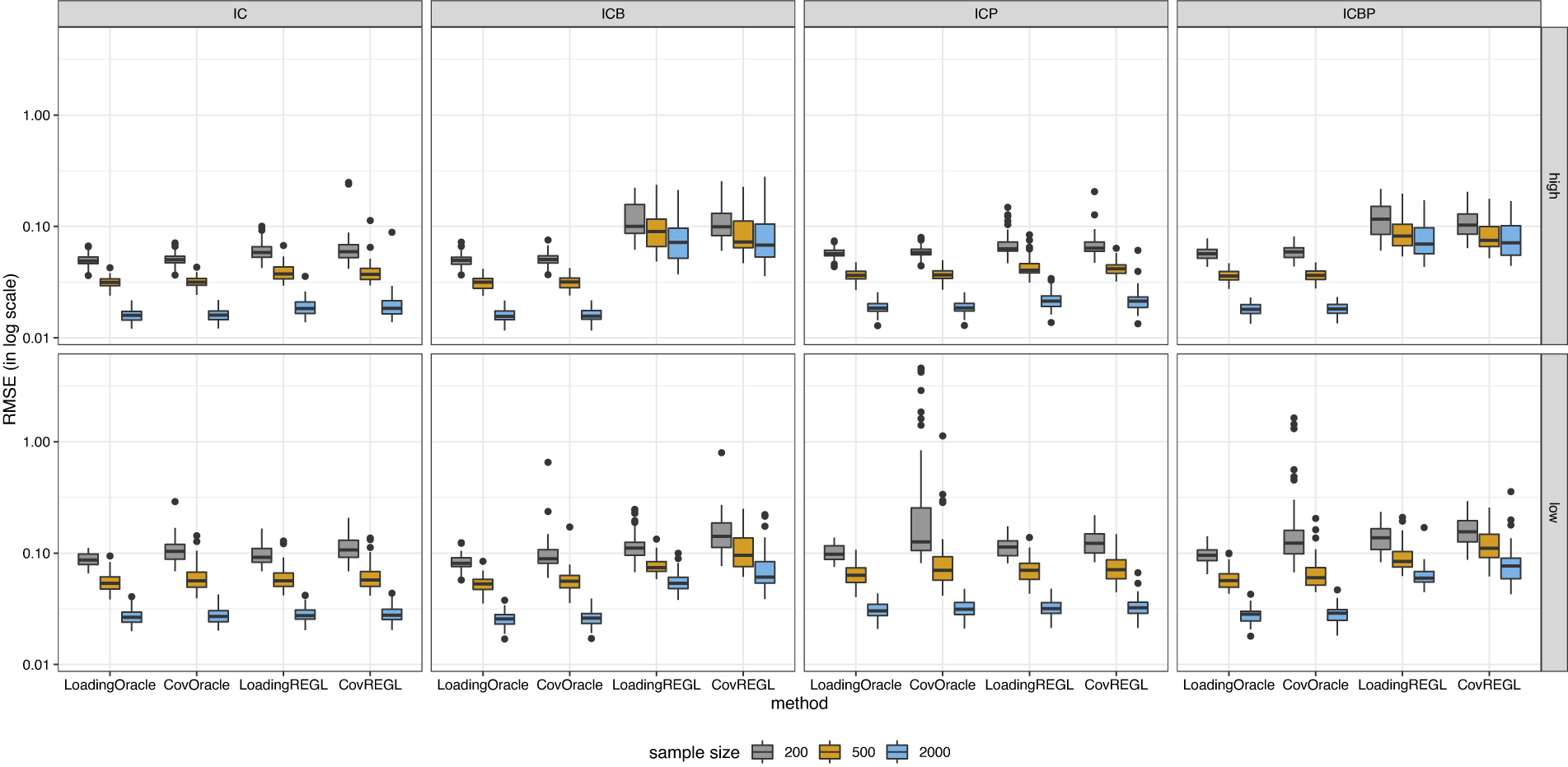
Figure A.3 Boxplot of the estimation error for loading matrix under semi-oblique bi-factor models.
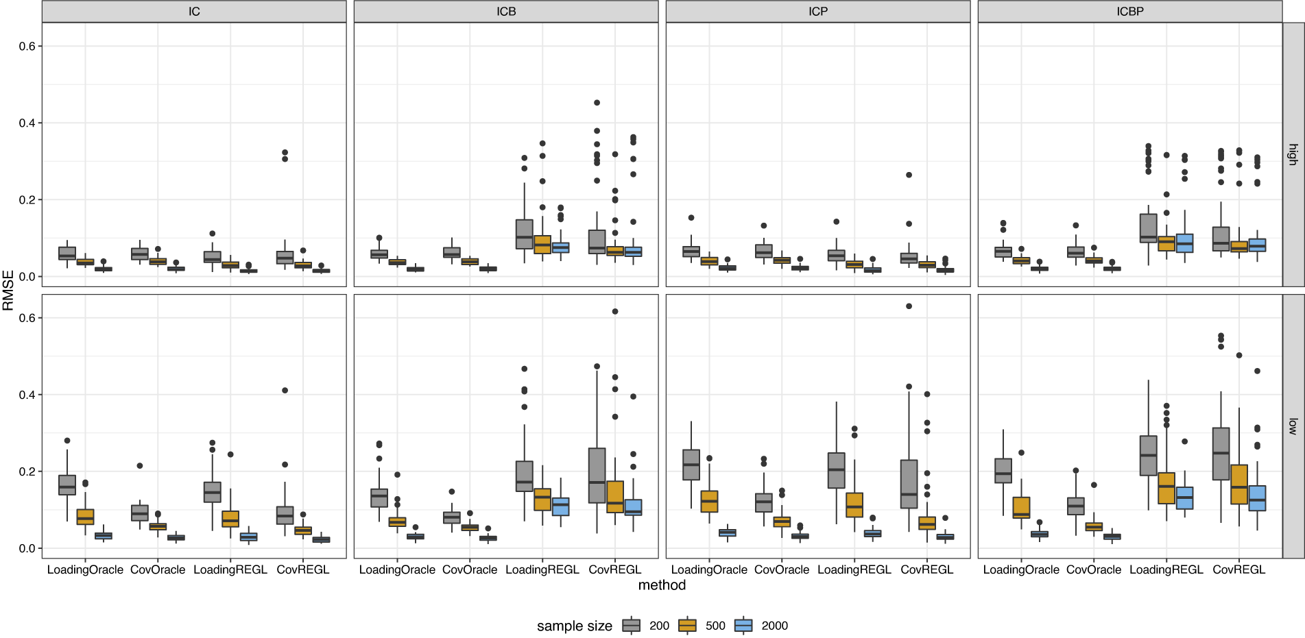
Figure A.4 Boxplot of the estimation error for factor correlation matrix under semi-oblique bi-factor models.
The pattern follows for the two practical methods, CovREGL (A.6) and LoadingREGL (A.5). These methods perform comparably in estimating the loading matrix when the loadings are high, but CovREGL shows slightly worse performance when the loadings are low. For factor correlation matrix estimation, the two methods are comparable when the loadings are high, but CovREGL outperforms LoadingREGL when the loadings are low, particularly under IC and ICP conditions. However, under ICB and ICBP conditions, the advantage of CovREGL over LoadingREGL in estimating the correlation matrix diminishes. This deterioration is likely due to model misspecification, as $\Lambda \not \in \mathcal {S}_{\mathrm {bi}}$
under these conditions. Surprisingly, CovREGL occasionally outperforms its oracle counterpart under IC and ICP conditions. In particular, the issue of extreme bias observed with CovOracle is no longer present with CovREGL.
$\Lambda \not \in \mathcal {S}_{\mathrm {bi}}$
under these conditions. Surprisingly, CovREGL occasionally outperforms its oracle counterpart under IC and ICP conditions. In particular, the issue of extreme bias observed with CovOracle is no longer present with CovREGL.


 Open access