


1. Introduction
Let $T \approx \mathbb{R}^2/\mathbb{Z}^2$
be the closed oriented surface of genus one. We indicate the homotopy class of an embedding of
$T \approx \mathbb{R}^2/\mathbb{Z}^2$
be the closed oriented surface of genus one. We indicate the homotopy class of an embedding of $S^1$
briefly by ‘curve’. By pulling a curve tight and lifting it to the universal cover, the collection of curves on T is in one-to-one correspondence with slopes
$S^1$
briefly by ‘curve’. By pulling a curve tight and lifting it to the universal cover, the collection of curves on T is in one-to-one correspondence with slopes $\mathbb{Q} \cup \{\infty\}$
. From this vantage point, the intersection number of a pair of curves on T (that is, the minimum possible number of intersection points among representatives from the pair of homotopy classes) can be computed explicitly via
$\mathbb{Q} \cup \{\infty\}$
. From this vantage point, the intersection number of a pair of curves on T (that is, the minimum possible number of intersection points among representatives from the pair of homotopy classes) can be computed explicitly via
 \begin{equation*}\iota\left( \frac pq , \frac ab\right) = \ | \ pb-qa \ | \ .\end{equation*}
A collection of curves is called a k-system when any pair of curves has intersection number at most k.
Let $\eta_S(k)$
equal the maximum size of a k-system on the closed surface S. It was first shown by [
Reference Juvan, Malnič and Mohar20
] that
$\eta_S(k)$
equal the maximum size of a k-system on the closed surface S. It was first shown by [
Reference Juvan, Malnič and Mohar20
] that $\eta_S(k)$
goes to infinity with k. The determination of the growth rate of
$\eta_S(k)$
goes to infinity with k. The determination of the growth rate of $\eta_S(k)$
, as a function of both k and the genus g of S, is a subtle counting problem, about which much remains unknown [
Reference Aougab, Biringer and Gaster1, Reference Aougab5, Reference Greene16, Reference Greene17, Reference Przytycki24
]. Notably, Greene has used probabilistic methods, leveraging the hyperbolic geometric bounds of Przytycki, to obtain
$\eta_S(k)$
, as a function of both k and the genus g of S, is a subtle counting problem, about which much remains unknown [
Reference Aougab, Biringer and Gaster1, Reference Aougab5, Reference Greene16, Reference Greene17, Reference Przytycki24
]. Notably, Greene has used probabilistic methods, leveraging the hyperbolic geometric bounds of Przytycki, to obtain $\eta_S(k) =O( g^{k+1}\log g)$
, when k is fixed and g grows [
Reference Greene16
, Theorem 3].
$\eta_S(k) =O( g^{k+1}\log g)$
, when k is fixed and g grows [
Reference Greene16
, Theorem 3].
For the study of $\eta_S(k)$
with g fixed, the simplest nontrivial case is evidently
$\eta_S(k)$
with g fixed, the simplest nontrivial case is evidently $S=T$
. A simple
$S=T$
. A simple $\mathrm{mod} \;p$
counting argument, as far as we know first observed by Agol, demonstrates that
$\mathrm{mod} \;p$
counting argument, as far as we know first observed by Agol, demonstrates that $\eta_T(k)$
is at most one more than the smallest prime greater than k [
Reference Agol4
]. Together with the elementary observation
$\eta_T(k)$
is at most one more than the smallest prime greater than k [
Reference Agol4
]. Together with the elementary observation $\eta_T(k)\ge k+2$
and the Prime Number Theorem, this implies
$\eta_T(k)\ge k+2$
and the Prime Number Theorem, this implies ${\eta_T(k)}/k \to 1$
as
${\eta_T(k)}/k \to 1$
as $k\to \infty$
[
Reference Agol3
].
$k\to \infty$
[
Reference Agol3
].
More can be said. The size of prime gaps, large and small, is a major field of study. The currently best upper bound is due to Baker–Harman–Pintz, which, together with Agol’s observation, implies that $\eta_T(k) = k+O(k^{21/40})$
[
Reference Baker, Harman and Pintz7
]. Cramér showed that a positive resolution of the Riemann hypothesis would provide
$\eta_T(k) = k+O(k^{21/40})$
[
Reference Baker, Harman and Pintz7
]. Cramér showed that a positive resolution of the Riemann hypothesis would provide $\eta_T(k) = k + O(\sqrt k \log k)$
[
Reference Cramér10
], and he formulated a stronger conjecture that would imply
$\eta_T(k) = k + O(\sqrt k \log k)$
[
Reference Cramér10
], and he formulated a stronger conjecture that would imply $\eta_T(k) = k+O((\log k)^2)$
[
Reference Cramér11
]; although there seems to be general suspicion in the analytic number theory community that Cramér’s error term should be replaced by
$\eta_T(k) = k+O((\log k)^2)$
[
Reference Cramér11
]; although there seems to be general suspicion in the analytic number theory community that Cramér’s error term should be replaced by $O((\log k)^{2+\epsilon})$
[
Reference Granville15, Reference Oliveira e Silva, Herzog and Pardi22
].
$O((\log k)^{2+\epsilon})$
[
Reference Granville15, Reference Oliveira e Silva, Herzog and Pardi22
].
All of these estimates pass through Agol’s remarkable prime number bound, but it is reasonable to be skeptical about whether estimation of $\eta_T(k)$
should depend on such notoriously subtle and difficult questions. The purpose of this paper is to sharpen currently available estimates, without reference to fine data about the distribution of the primes. Our methods are elementary, combinatorial and hyperbolic.
$\eta_T(k)$
should depend on such notoriously subtle and difficult questions. The purpose of this paper is to sharpen currently available estimates, without reference to fine data about the distribution of the primes. Our methods are elementary, combinatorial and hyperbolic.
Theorem 1·1. There is a constant $C>0$
so that
$C>0$
so that $\eta_T(k)\le k+C\sqrt k \log k$
.
$\eta_T(k)\le k+C\sqrt k \log k$
.
As for sharpness, it deserves remarking that there is a dearth of nontrivial lower bounds for $\eta_T(k)$
. In fact, we are unaware of any example of a k-system of size
$\eta_T(k)$
. In fact, we are unaware of any example of a k-system of size $k+7$
on the torus (cf. [
Reference Gaster, Lopez, Rexer, Riell and Xiao14
, p. 116]).
$k+7$
on the torus (cf. [
Reference Gaster, Lopez, Rexer, Riell and Xiao14
, p. 116]).
The function $\eta_T(k)$
admits a dual formulation: let
$\eta_T(k)$
admits a dual formulation: let $\kappa_S(n)$
indicate the minimum, taken over collections of n curves on S, of the maximum pairwise intersection. (For clarity, we will often use ‘n’ to indicate the size of a set of curves and ‘k’ for an intersection number.) It is not hard to see that
$\kappa_S(n)$
indicate the minimum, taken over collections of n curves on S, of the maximum pairwise intersection. (For clarity, we will often use ‘n’ to indicate the size of a set of curves and ‘k’ for an intersection number.) It is not hard to see that
 \begin{equation*}\eta_S(k) = \max \{ n\;:\; \kappa_S(n) \le k\} \ , \text{ and } \ \kappa_S(n) = \min \{k\; :\; \eta_S(k)\ge n\}.\end{equation*}
Our path towards Theorem 1·1 will be to first estimate $\kappa_T(n)$
from below.
$\kappa_T(n)$
from below.
There is a kind of convexity to exploit in the study of $\kappa_T$
, originally observed by Agol. As remarked above, curves on T are in correspondence with slopes
$\kappa_T$
, originally observed by Agol. As remarked above, curves on T are in correspondence with slopes $\mathbb{Q}\cup \{\infty\}$
. The latter form the vertices of the Farey complex
$\mathbb{Q}\cup \{\infty\}$
. The latter form the vertices of the Farey complex $\mathcal{F}$
, in which a set of slopes form a simplex when they pairwise intersect once. Any collection of n curves that is maximal with respect to inclusion among k-systems determines a collection of vertices in
$\mathcal{F}$
, in which a set of slopes form a simplex when they pairwise intersect once. Any collection of n curves that is maximal with respect to inclusion among k-systems determines a collection of vertices in $\mathcal{F}$
so that the induced simplicial complex is a triangulated n-gon (see Lemma 2·4 for detail).
$\mathcal{F}$
so that the induced simplicial complex is a triangulated n-gon (see Lemma 2·4 for detail).
Conversely, any triangulation of an n-gon can be realised as a subcomplex of $\mathcal{F}$
, in a way that is unique up to the action of
$\mathcal{F}$
, in a way that is unique up to the action of $\mathrm{PSL}(2,\mathbb{Z}) \curvearrowright \mathcal{F}$
by simplicial automorphism. As
$\mathrm{PSL}(2,\mathbb{Z}) \curvearrowright \mathcal{F}$
by simplicial automorphism. As $\mathrm{PSL}(2,\mathbb{Z})$
preserves the intersection form, the (multi-)set of pairwise intersection numbers is a well-defined function on the set of triangulations of an n-gon. The set of triangulations of an n-gon forms the vertex set of a well-studied simplicial complex in combinatorics called the associahedron
$\mathrm{PSL}(2,\mathbb{Z})$
preserves the intersection form, the (multi-)set of pairwise intersection numbers is a well-defined function on the set of triangulations of an n-gon. The set of triangulations of an n-gon forms the vertex set of a well-studied simplicial complex in combinatorics called the associahedron $\mathcal{A}_n$
(there is a slight indexing issue; the object we refer to as
$\mathcal{A}_n$
(there is a slight indexing issue; the object we refer to as $\mathcal{A}_n$
is the
$\mathcal{A}_n$
is the $(n-2)$
-dimensional associahedron). One obtains a ‘max intersection’ function
$(n-2)$
-dimensional associahedron). One obtains a ‘max intersection’ function $\kappa\;:\; \mathcal{A}_n \to \mathbb{N}$
induced by the intersection form on
$\kappa\;:\; \mathcal{A}_n \to \mathbb{N}$
induced by the intersection form on $\mathcal{F}$
, and the above discussion leads to
$\mathcal{F}$
, and the above discussion leads to $\kappa_T(n)=\min \kappa$
(see Proposition 2·5).
$\kappa_T(n)=\min \kappa$
(see Proposition 2·5).
Theorem 1·1 follows from the following:
Theorem 1·2. There is a constant $C>0$
so that, for any
$C>0$
so that, for any $\tau\in \mathcal{A}_n$
, we have
$\tau\in \mathcal{A}_n$
, we have $\kappa(\tau) \ge n - C \sqrt n \log n $
.
$\kappa(\tau) \ge n - C \sqrt n \log n $
.
We briefly describe the proof of this theorem. The Farey complex $\mathcal{F}$
admits a natural embedding into a compactification of the hyperbolic plane
$\mathcal{F}$
admits a natural embedding into a compactification of the hyperbolic plane $\mathbb{H}^2 \,\cup\, \partial_\infty \mathbb{H}^2$
, so that the vertices of
$\mathbb{H}^2 \,\cup\, \partial_\infty \mathbb{H}^2$
, so that the vertices of $\mathcal{F}$
embed naturally as
$\mathcal{F}$
embed naturally as $\mathbb{Q} \cup\{\infty\} \hookrightarrow \mathbb{R}\cup\{\infty\} \approx \partial_\infty \mathbb{H}^2$
, with edges between vertices mapping to geodesics. The hyperbolic plane
$\mathbb{Q} \cup\{\infty\} \hookrightarrow \mathbb{R}\cup\{\infty\} \approx \partial_\infty \mathbb{H}^2$
, with edges between vertices mapping to geodesics. The hyperbolic plane $\mathbb{H}^2$
admits a maximal
$\mathbb{H}^2$
admits a maximal $\mathrm{PSL}(2,\mathbb{Z})$
-invariant horospherical packing
$\mathrm{PSL}(2,\mathbb{Z})$
-invariant horospherical packing $\{H_{p/q}\;:\; p/q \in \mathbb{Q}\cup\{\infty\}\}$
, where
$\{H_{p/q}\;:\; p/q \in \mathbb{Q}\cup\{\infty\}\}$
, where $H_{p/q}$
is centered at
$H_{p/q}$
is centered at $p/q\in \mathbb{R}\cup\{\infty\}$
, so that a set of slopes span a simplex in
$p/q\in \mathbb{R}\cup\{\infty\}$
, so that a set of slopes span a simplex in $\mathcal{F}$
precisely when the corresponding horospheres are pairwise tangent. (The nomenclature for
$\mathcal{F}$
precisely when the corresponding horospheres are pairwise tangent. (The nomenclature for $H_{p/q}$
is standard in hyperbolic geometry [
Reference Thurston29
, Chapter 3] – these are also called Ford circles in the literature [
Reference Conway and Guy8, Reference Bonahon12, Reference Ford13
]).
$H_{p/q}$
is standard in hyperbolic geometry [
Reference Thurston29
, Chapter 3] – these are also called Ford circles in the literature [
Reference Conway and Guy8, Reference Bonahon12, Reference Ford13
]).
A sketch of our proof of Theorem 1·2 is as follows:
-
(i) locate a ‘nice horoball’ H for $\tau$
, so that
$\mathrm{ht}(\tau,H)$
, the height of
$\tau$
relative to H, is
$O\!\left(\sqrt{\kappa(\tau)}\right)$
. See Definition 3 and Proposition 5·1;
$\tau$
, so that
$\mathrm{ht}(\tau,H)$
, the height of
$\tau$
relative to H, is
$O\!\left(\sqrt{\kappa(\tau)}\right)$
. See Definition 3 and Proposition 5·1; -
(ii) use H to construct a convex combination of pairwise intersection numbers for
$\tau$
whose sum is at least
$n - O(h \log h)$
, where
$h= \mathrm{ht}(\tau,H)$
. It follows that there is a pair of horoballs of
$\tau$
with intersection number at least
$n-O(h \log h)$
. See Proposition 4·2.


The proof of Theorem 1·2 is now immediate: if $\kappa(\tau)\le n$
, then
$\kappa(\tau)\le n$
, then $\kappa(\tau) \ge n-C \sqrt n \log n$
.
$\kappa(\tau) \ge n-C \sqrt n \log n$
.
The first step above uses the hyperbolic geometry of $\mathbb{H}^2$
in an essential way, in which we exploit a simple relationship between intersection numbers, hyperbolic geometry, and Ford circles (see Lemma 2·3).
$\mathbb{H}^2$
in an essential way, in which we exploit a simple relationship between intersection numbers, hyperbolic geometry, and Ford circles (see Lemma 2·3).
Organisation. We describe the reduction from $\kappa_T(n)$
to
$\kappa_T(n)$
to $\kappa\;:\;\mathcal{A}_n\to\mathbb{N}$
in Section 2, analyse several examples in Section 3, bound
$\kappa\;:\;\mathcal{A}_n\to\mathbb{N}$
in Section 2, analyse several examples in Section 3, bound $\kappa(\tau)$
from below in Section 4, locate a good horoball for
$\kappa(\tau)$
from below in Section 4, locate a good horoball for $\tau$
in Section 5, and prove Theorem 1·1 in Section 6.
$\tau$
in Section 5, and prove Theorem 1·1 in Section 6.
2. Preliminaries
We collect here some useful facts about intersection numbers and the Farey graph $\mathcal{F}$
. For more of the beautiful connections between hyperbolic geometry, the Farey graph, continued fractions, and Diophantine approximation, we suggest the reader consult [
Reference Hatcher18, Reference Series25, Reference Series26, Reference Springborn27
].
$\mathcal{F}$
. For more of the beautiful connections between hyperbolic geometry, the Farey graph, continued fractions, and Diophantine approximation, we suggest the reader consult [
Reference Hatcher18, Reference Series25, Reference Series26, Reference Springborn27
].
2·1. Horoballs in trees, Farey labellings, and intersection numbers
Dual to a triangulation of an n-gon $\tau\in\mathcal{A}_n$
there is a trivalent tree with n leaves embedded in the plane, which we refer to as
$\tau\in\mathcal{A}_n$
there is a trivalent tree with n leaves embedded in the plane, which we refer to as $\tau^*$
. Because
$\tau^*$
. Because $\tau^*$
is embedded in the plane, the three edges incident to vertices of
$\tau^*$
is embedded in the plane, the three edges incident to vertices of $\tau^*$
are cyclically ordered. Hence any non-backtracking path in
$\tau^*$
are cyclically ordered. Hence any non-backtracking path in $\tau^*$
induces a sequence of left-right turns.
$\tau^*$
induces a sequence of left-right turns.
The vertices of $\tau$
(that is, the slopes of the k-system) correspond to ‘horoballs’ in
$\tau$
(that is, the slopes of the k-system) correspond to ‘horoballs’ in $\tau^*$
:
$\tau^*$
:
Definition 1 (Horoballs in trees). A horoball is a union of edges in a path of the dual tree $\tau^*$
that is composed of uni-directional turns (that is, only left or only right turns), which is moreover maximal with respect to inclusion among all such uni-directional subsets of
$\tau^*$
that is composed of uni-directional turns (that is, only left or only right turns), which is moreover maximal with respect to inclusion among all such uni-directional subsets of $\tau^*$
.
$\tau^*$
.
Note that horoballs may be alternately considered as subsets of $\tau$
,
$\tau$
, $\tau^*$
, or
$\tau^*$
, or $\mathbb{H}^2$
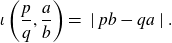
. We leave the intended meaning to be implied contextually. See Figure 1 for an illustration.
$\mathbb{H}^2$
. We leave the intended meaning to be implied contextually. See Figure 1 for an illustration.
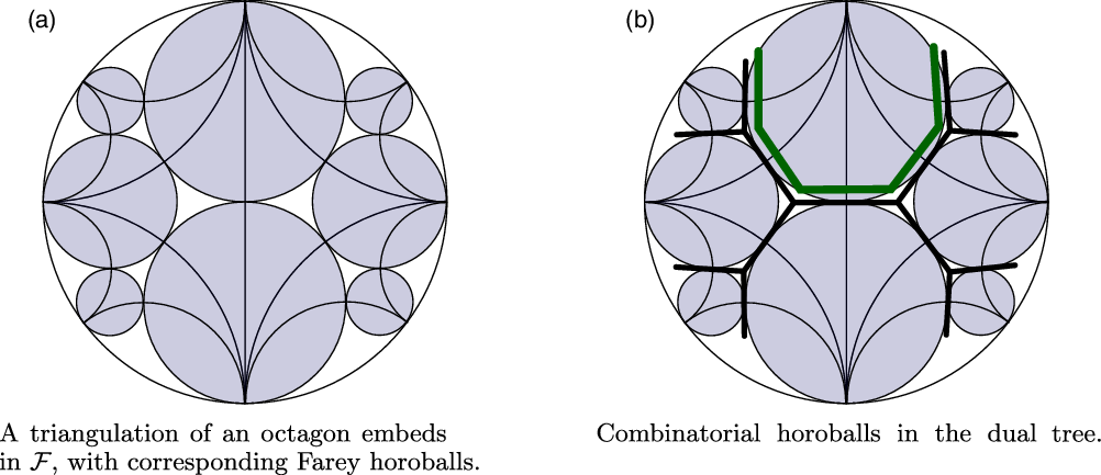
Fig. 1. Horoballs in $\mathbb{H}^2$
and horoballs in trees.
$\mathbb{H}^2$
and horoballs in trees.
A triangulation $\tau\in\mathcal{A}_n$
admits an embedding into
$\tau\in\mathcal{A}_n$
admits an embedding into $\mathcal{F}$
, and any such embedding gives a map from horoballs of
$\mathcal{F}$
, and any such embedding gives a map from horoballs of $\tau$
to
$\tau$
to $\mathbb{Q}\cup \{\infty\}$
that records the center of the corresponding horoball in
$\mathbb{Q}\cup \{\infty\}$
that records the center of the corresponding horoball in $\mathbb{H}^2$
.
$\mathbb{H}^2$
.
Definition 2 (Farey labellings and intersection numbers). A Farey labelling of $\tau$
is the map from horoballs to
$\tau$
is the map from horoballs to $\mathbb{Q} \cup \{\infty\}$
obtained from an embedding of
$\mathbb{Q} \cup \{\infty\}$
obtained from an embedding of $\tau$
in
$\tau$
in $\mathcal{F}$
. The intersection number
$\mathcal{F}$
. The intersection number $\iota(H_1,H_2)$
of a pair of horoballs
$\iota(H_1,H_2)$
of a pair of horoballs $H_1$
and
$H_1$
and $H_2$
is given by the intersection number of the slopes corresponding to
$H_2$
is given by the intersection number of the slopes corresponding to $H_1$
and
$H_1$
and $H_2$
in a Farey labelling of
$H_2$
in a Farey labelling of $\tau$
.
$\tau$
.
We refer to the introduction for an explanation of why intersection numbers of $\tau$
are well-defined.
$\tau$
are well-defined.
Farey labellings are especially pleasant because the vertices spanning a simplex of $\mathcal{F}$
satisfy a remarkably simple relationship. Namely, if
$\mathcal{F}$
satisfy a remarkably simple relationship. Namely, if $p/q$
and
$p/q$
and $a/b$
span an edge of
$a/b$
span an edge of $\mathcal{F}$
, then the two other vertices of
$\mathcal{F}$
, then the two other vertices of $\mathcal{F}$
that span a triangle with
$\mathcal{F}$
that span a triangle with $p/q$
and
$p/q$
and $a/b$
are
$a/b$
are ${(p+ a)}/{(q+ b)}$
and
${(p+ a)}/{(q+ b)}$
and ${(p-a)}/{(q-b)}$
; this is the ‘Farey addition’ rule. Note that the choice of labels
${(p-a)}/{(q-b)}$
; this is the ‘Farey addition’ rule. Note that the choice of labels $1/0$
,
$1/0$
, $0/1$
, and
$0/1$
, and $1/1$
for three horoballs incident to a non-leaf vertex of
$1/1$
for three horoballs incident to a non-leaf vertex of $\tau^*$
induces a Farey labelling by using Farey addition to deduce labels of neighbouring horoballs.
$\tau^*$
induces a Farey labelling by using Farey addition to deduce labels of neighbouring horoballs.
2·2. Monotonicity of intersection numbers and left-right sequences
The intersection number $\iota(H_1,H_2)$
admits a description more intrinsic to the structure of
$\iota(H_1,H_2)$
admits a description more intrinsic to the structure of $\tau^*$
, which we now describe. There is a unique (possibly degenerate) non-backtracking path
$\tau^*$
, which we now describe. There is a unique (possibly degenerate) non-backtracking path $\sigma$
between the pair of horoballs
$\sigma$
between the pair of horoballs $H_1$
and
$H_1$
and $H_2$
, and this path determines a sequence of left-right turns
$H_2$
, and this path determines a sequence of left-right turns $(\ell_1,\ell_2,\ldots,\ell_s)$
, where
$(\ell_1,\ell_2,\ldots,\ell_s)$
, where $\sigma$
makes
$\sigma$
makes $\ell_1$
turns in the same direction, followed by
$\ell_1$
turns in the same direction, followed by $\ell_2$
turns in the opposite direction, etc. The quantity
$\ell_2$
turns in the opposite direction, etc. The quantity $\iota(H_1,H_2)$
is given by the numerator of the continued fraction with coefficients
$\iota(H_1,H_2)$
is given by the numerator of the continued fraction with coefficients $(\ell_1,\ell_2,\ldots,\ell_s)$
[
Reference Gaster, Lopez, Rexer, Riell and Xiao14
, Theorem 5·3].
$(\ell_1,\ell_2,\ldots,\ell_s)$
[
Reference Gaster, Lopez, Rexer, Riell and Xiao14
, Theorem 5·3].
Remark. Observe that there is ambiguity in this computation of $\iota(H_1,H_2)$
. For one, the non-backtracking path
$\iota(H_1,H_2)$
. For one, the non-backtracking path $\sigma$
may go either from
$\sigma$
may go either from $H_1$
to
$H_1$
to $H_2$
, or from
$H_2$
, or from $H_2$
to
$H_2$
to $H_1$
. Moreover, one must declare that
$H_1$
. Moreover, one must declare that $\sigma$
is starting with either ‘left’ or ‘right’ at its origin vertex, so that it can be observed whether
$\sigma$
is starting with either ‘left’ or ‘right’ at its origin vertex, so that it can be observed whether $\sigma$
is switching directions or not at later vertices. These choices may be made arbitrarily and independently, and this ambiguity has no affect on the calculation of
$\sigma$
is switching directions or not at later vertices. These choices may be made arbitrarily and independently, and this ambiguity has no affect on the calculation of $\iota(H_1,H_2)$
. See [
Reference Gaster, Lopez, Rexer, Riell and Xiao14
, figure 3, example 1].
$\iota(H_1,H_2)$
. See [
Reference Gaster, Lopez, Rexer, Riell and Xiao14
, figure 3, example 1].
This viewpoint suggests a certain monotonicity.
Lemma 2·1 (‘Monotonicity of intersection numbers’). Suppose that $\sigma$
and
$\sigma$
and $\sigma'$
are non-backtracking paths with respective left-right sequences
$\sigma'$
are non-backtracking paths with respective left-right sequences $(\ell_1,\ldots,\ell_s)$
and
$(\ell_1,\ldots,\ell_s)$
and $(\ell'_{\!\!1},\ldots,\ell'_{\!\!s'})$
. If
$(\ell'_{\!\!1},\ldots,\ell'_{\!\!s'})$
. If $s'\ge s$
and
$s'\ge s$
and $\ell_i'\ge \ell_i$
for each
$\ell_i'\ge \ell_i$
for each $i=1,\ldots,s$
, then the intersection number determined by
$i=1,\ldots,s$
, then the intersection number determined by $\sigma'$
is at least that determined by
$\sigma'$
is at least that determined by $\sigma$
.
$\sigma$
.
Proof. This lemma is almost exactly [
Reference Gaster, Lopez, Rexer, Riell and Xiao14
, lemma 5·5], with the sole difference that we may have $s'>s$
. Therefore to prove the claim we may assume that
$s'>s$
. Therefore to prove the claim we may assume that $\sigma'$
contains
$\sigma'$
contains $\sigma$
as an initial subpath.
$\sigma$
as an initial subpath.
Choose a Farey labelling with label $1/0$
at the horoball forming the origin of
$1/0$
at the horoball forming the origin of $\sigma$
(and
$\sigma$
(and $\sigma'$
), and labels
$\sigma'$
), and labels $0/1$
and
$0/1$
and $1/1$
at the two neighbouring horoballs that intersect
$1/1$
at the two neighbouring horoballs that intersect $\sigma$
. Compare the denominators of the Farey labels of the horoballs at the terminuses of
$\sigma$
. Compare the denominators of the Farey labels of the horoballs at the terminuses of $\sigma$
and
$\sigma$
and $\sigma'$
; because these labels are computed using Farey addition, it is evident that the denominator of the horoball for
$\sigma'$
; because these labels are computed using Farey addition, it is evident that the denominator of the horoball for $\sigma'$
is at least that of
$\sigma'$
is at least that of $\sigma$
. The intersection number of any horoball with
$\sigma$
. The intersection number of any horoball with $1/0$
is given by the denominator of its Farey label, so the claim follows.
$1/0$
is given by the denominator of its Farey label, so the claim follows.
2·3. Intersection numbers and hyperbolic distance
The quotient of $\mathbb{H}^2$
by
$\mathbb{H}^2$
by $\mathrm{PSL}(2,\mathbb{Z})$
is a hyperbolic orbifold with one cusp and two orbifold points, one of order 2 and one of order 3. The preimage of the maximal horoball neighborhood of the cusp under the covering projection
$\mathrm{PSL}(2,\mathbb{Z})$
is a hyperbolic orbifold with one cusp and two orbifold points, one of order 2 and one of order 3. The preimage of the maximal horoball neighborhood of the cusp under the covering projection $\mathbb{H}^2 \to \mathbb{H}^2/\mathrm{PSL}(2,\mathbb{Z})$
is
$\mathbb{H}^2 \to \mathbb{H}^2/\mathrm{PSL}(2,\mathbb{Z})$
is $\mathcal{H}=\{H_{p/q}\;:\;p/q\in\mathbb{Q}\cup\{\infty\}\}$
, a
$\mathcal{H}=\{H_{p/q}\;:\;p/q\in\mathbb{Q}\cup\{\infty\}\}$
, a $\mathrm{PSL}(2,\mathbb{Z})$
-invariant collection of horoballs centered at the completed rationals. The following lemma is an exercise in hyperbolic geometry.
$\mathrm{PSL}(2,\mathbb{Z})$
-invariant collection of horoballs centered at the completed rationals. The following lemma is an exercise in hyperbolic geometry.
Lemma 2·2. Every point in $\mathbb{H}^2$
is within
$\mathbb{H}^2$
is within $\log 2/{\sqrt 3}$
of a horoball in
$\log 2/{\sqrt 3}$
of a horoball in $\mathcal{H}$
.
$\mathcal{H}$
.
There is a simple well-known fundamental relationship between intersection numbers of curves on the torus and hyperbolic distance between the corresponding horoballs (see e.g. [ Reference Springborn27 , proposition 6·2]).
Lemma 2·3. We have $\displaystyle d_{\mathbb{H}^2}\left(H_{p/q},H_{a/b} \right) =2 \log \iota\left( \frac pq , \frac ab \right) $
for any
$\displaystyle d_{\mathbb{H}^2}\left(H_{p/q},H_{a/b} \right) =2 \log \iota\left( \frac pq , \frac ab \right) $
for any $p/q, a/b \in \mathcal{F}$
.
$p/q, a/b \in \mathcal{F}$
.
Proof. Applying an element of $\mathrm{PSL}(2,\mathbb{Z})$
, we may assume that
$\mathrm{PSL}(2,\mathbb{Z})$
, we may assume that $p/q=\infty$
in the upper half-plane model for
$p/q=\infty$
in the upper half-plane model for $\mathbb{H}^2 \, \cup \, \partial_\infty \mathbb{H}^2$
. The horosphere
$\mathbb{H}^2 \, \cup \, \partial_\infty \mathbb{H}^2$
. The horosphere $H_{a/b}$
is given by
$H_{a/b}$
is given by $\{z\;:\; \left| z-(a/b + i/{2b^2}) \right| = 1/{2b^2}\}$
(see e.g. [
Reference Athreya, Chaubey, Malik and Zaharescu2
]), so
$\{z\;:\; \left| z-(a/b + i/{2b^2}) \right| = 1/{2b^2}\}$
(see e.g. [
Reference Athreya, Chaubey, Malik and Zaharescu2
]), so
 \begin{equation*}d_{\mathbb{H}^2}\left(H_{p/q},H_{a/b} \right) =d_{\mathbb{H}^2}\left( a/b + \frac i{b^2} , a/b + i\right) = 2\log b = 2 \log \iota\left( \frac pq , \frac ab \right) .\end{equation*}
2·4. Width and height for horoballs
The interior of each edge of $\tau^*$
is incident to exactly two horoball regions. Thus, for any choice of horoball H in
$\tau^*$
is incident to exactly two horoball regions. Thus, for any choice of horoball H in $\tau^*$
, there are exactly two other horoball regions, distinct from H, that are incident to the interiors of the extreme edges of H. Call these
$\tau^*$
, there are exactly two other horoball regions, distinct from H, that are incident to the interiors of the extreme edges of H. Call these $H_1$
and
$H_1$
and $H_2$
.
$H_2$
.
Definition 3. The width of $\tau$
relative to H is
$\tau$
relative to H is $w = \iota(H_1,H_2)$
. The height of
$w = \iota(H_1,H_2)$
. The height of $\tau$
relative to H is
$\tau$
relative to H is
 \begin{equation*}\mathrm{ht}(\tau,H) =\max \{ \ \iota(H, H') \ :\; H' \text{ is a horoball of }\tau \ \}.\end{equation*}
For the remainder of this article, we will suppress the difference between the triangulation $\tau\in\mathcal{A}_n$
and its dual tree
$\tau\in\mathcal{A}_n$
and its dual tree $\tau^*$
. The translation between them is quite natural, and the difference can henceforth be understood from context.
$\tau^*$
. The translation between them is quite natural, and the difference can henceforth be understood from context.
2·5. The two kappas
Recall from the introduction the quantity $\kappa_T(n)$
, which is the minimum, taken over collections
$\kappa_T(n)$
, which is the minimum, taken over collections $\Gamma$
of n curves on S, of the maximum pairwise intersection number of curves in
$\Gamma$
of n curves on S, of the maximum pairwise intersection number of curves in $\Gamma$
.
$\Gamma$
.
Definition 4 (‘Max Intersection Function’). The function $\kappa\;:\;\mathcal{A}_n\to \mathbb{N}$
is defined by
$\kappa\;:\;\mathcal{A}_n\to \mathbb{N}$
is defined by
 \begin{equation*}\kappa(\tau) = \max\{\ \iota(H_1,H_2) \;:\; H_1 \text{ and }H_2 \text{ are horoballs of }\tau \ \}.\end{equation*}
As noted in the introduction, we claim that $\kappa_T(n)= \min \{ \kappa(\tau)\;:\; \tau\in \mathcal{A}_n \}$
.
$\kappa_T(n)= \min \{ \kappa(\tau)\;:\; \tau\in \mathcal{A}_n \}$
.
That $\kappa_T(n)\le \min \kappa$
is easy: for any
$\kappa_T(n)\le \min \kappa$
is easy: for any $\tau\in\mathcal{A}_n$
, choose a Farey labelling. The quantity
$\tau\in\mathcal{A}_n$
, choose a Farey labelling. The quantity $\kappa(\tau)$
is equal to the maximum pairwise intersection number of the n slopes obtained in this Farey labelling, and
$\kappa(\tau)$
is equal to the maximum pairwise intersection number of the n slopes obtained in this Farey labelling, and $\kappa_T(n)$
is the minimum of the maximum pairwise intersection of any n slopes, so
$\kappa_T(n)$
is the minimum of the maximum pairwise intersection of any n slopes, so $\kappa_T(n) \le \kappa(\tau)$
for each
$\kappa_T(n) \le \kappa(\tau)$
for each $\tau\in\mathcal{A}_n$
.
$\tau\in\mathcal{A}_n$
.
The reverse inequality is slightly less obvious, and relies on a certain convexity of maximal k-systems in $\partial_\infty \mathbb{H}^2$
. The following lemma makes this precise.Footnote 1
$\partial_\infty \mathbb{H}^2$
. The following lemma makes this precise.Footnote 1
Lemma 2·4. If $\Gamma$
is a k-system on T which is maximal with respect to inclusion among k-systems, then
$\Gamma$
is a k-system on T which is maximal with respect to inclusion among k-systems, then $\mathcal{F}$
induces a triangulation of the n-gon which forms the convex hull of
$\mathcal{F}$
induces a triangulation of the n-gon which forms the convex hull of $\Gamma\subset \partial_\infty \mathbb{H}^2$
.
$\Gamma\subset \partial_\infty \mathbb{H}^2$
.
Proof. Let $g_{ab}$
indicate the geodesic in
$g_{ab}$
indicate the geodesic in $\mathbb{H}^2$
with endpoints
$\mathbb{H}^2$
with endpoints $a,b\in\partial_\infty \mathbb{H}^2$
. Suppose that
$a,b\in\partial_\infty \mathbb{H}^2$
. Suppose that $\alpha,\beta\in\Gamma\subset \mathcal{F}$
, that
$\alpha,\beta\in\Gamma\subset \mathcal{F}$
, that $\Delta$
is a Farey triangle intersecting
$\Delta$
is a Farey triangle intersecting $g_{\alpha\beta}$
, and that
$g_{\alpha\beta}$
, and that $\delta$
is a vertex of
$\delta$
is a vertex of $\Delta$
(and, hence, of
$\Delta$
(and, hence, of $\mathcal{F}$
). Because the path
$\mathcal{F}$
). Because the path $\sigma$
that computes the intersection number
$\sigma$
that computes the intersection number $\iota(\alpha,\delta)$
is a subpath of the path
$\iota(\alpha,\delta)$
is a subpath of the path $\sigma'$
that computes
$\sigma'$
that computes $\iota(\alpha, \beta)$
(and similarly for
$\iota(\alpha, \beta)$
(and similarly for $\iota(\delta,\beta)$
), Lemma 2·1 implies that both
$\iota(\delta,\beta)$
), Lemma 2·1 implies that both $\iota(\delta,\alpha)$
and
$\iota(\delta,\alpha)$
and $\iota(\delta,\beta)$
are at most k. For any
$\iota(\delta,\beta)$
are at most k. For any $\gamma\in\Gamma$
, either
$\gamma\in\Gamma$
, either $g_{\alpha\gamma}$
or
$g_{\alpha\gamma}$
or $g_{\beta\gamma}$
intersect
$g_{\beta\gamma}$
intersect $\Delta$
, so it follows that
$\Delta$
, so it follows that $\iota(\gamma,\delta)\le k$
as well. Maximality of
$\iota(\gamma,\delta)\le k$
as well. Maximality of $\Gamma$
implies that
$\Gamma$
implies that $\delta\in\Gamma$
, so the convex hull of
$\delta\in\Gamma$
, so the convex hull of $\Gamma$
is equal to the union of Farey triangles spanning elements of
$\Gamma$
is equal to the union of Farey triangles spanning elements of $\Gamma$
.
$\Gamma$
.
This demonstrates that $\kappa_T(n) \ge \min \kappa$
, so we may conclude:
$\kappa_T(n) \ge \min \kappa$
, so we may conclude:
Proposition 2·5. We have $\displaystyle \kappa_T(n) = \min_{\tau\in\mathcal{A}_n} \kappa$
.
$\displaystyle \kappa_T(n) = \min_{\tau\in\mathcal{A}_n} \kappa$
.
3. Illustrative examples
There are several natural elements of $\mathcal{A}_n$
that we can use to observe
$\mathcal{A}_n$
that we can use to observe $\kappa\;:\;\mathcal{A}_n\to \mathbb{N}$
.
$\kappa\;:\;\mathcal{A}_n\to \mathbb{N}$
.
Remark. Technically, the vertices of the associahedron correspond to triangulations of a labelled convex polygon. Notice however that the max intersection function $\kappa\;:\;\mathcal{A}_n\to\mathbb{N}$
is invariant under permutation of labels, so we can safely refer to
$\kappa\;:\;\mathcal{A}_n\to\mathbb{N}$
is invariant under permutation of labels, so we can safely refer to $\kappa(\tau)$
for elements
$\kappa(\tau)$
for elements $\tau$
of
$\tau$
of $\mathcal{A}_n$
without reference to a particular ordering of the horoballs of
$\mathcal{A}_n$
without reference to a particular ordering of the horoballs of $\tau$
.
$\tau$
.
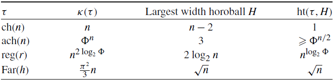
-
(i) The element
$\mathrm{ch}(n)\in\mathcal{A}_n$
(for ‘chain’) contains a horoball of width n. We have
$\kappa(\mathrm{ch}(n))=n$
, and the height relative to the horoball of width n is 1. -
(ii) The element
$\mathrm{ach}(n)\in\mathcal{A}_n$
(for ‘alternating chain’) contains a path of length
$n-3$
that switches direction
$n-4$
times. Here we have
$\kappa(\mathrm{ach}(n))=F_n$
, the nth Fibonacci number, the largest width horoball of
$\mathrm{ach}(n)$
is 3, and the height relative to any horoball is at least
$F_{\lfloor \frac n2\rfloor }$
. -
(iii) The element
$\mathrm{reg}(r)\in\mathcal{A}_n$
(for ‘regular’), with
$n=3\cdot 2^{r-1}$
, is formed by choosing the subtree of the homogeneous (infinite) trivalent tree that is induced on all vertices at combinatorial distance at most r from a fixed vertex. The tree
$\mathrm{reg}(r)$
contains the alternating chain
$\mathrm{ach}(2r+1)$
as a subtree, and in fact we have
$\kappa(\mathrm{reg}(r))=\kappa(\mathrm{ach}(2r+1))=F_{2r+1}$
. The largest width of a horoball of
$\mathrm{reg}(r)$
is given by
$2r-1$
, and the height of
$\mathrm{reg}(r)$
relative to this horoball is
$F_{r+1}$
. -
(iv) The element
$\mathrm{Far}(h)\in\mathcal{A}_n$
(for the ‘Farey series’), with
$n=2+\sum_{k\le h} \phi(k)$
, where
$\phi$
is Euler’s totient function, is the subgraph of
$\mathcal{F}$
induced on fractions in
$\mathbb{Q}\cap [0,1]$
that can be written with denominator
$\le h$
, together with
$1/0$
. Observe that
$\kappa(\mathrm{Far}(h)) =h^2-2h$
, the largest width of a horoball of
$\mathrm{Far}(h)$
is given by h, while the height relative to this horoball is given by
$h-1$
.


We collect this information in Figure 2 and Table 1.
Fig. 2. Several dual trees of elements in $\mathcal{A}_n$
.
$\mathcal{A}_n$
.
Remark. Observe the large difference between $\kappa(\mathrm{ach}(n))\approx (({1+\sqrt5})/2)^n$
and
$\kappa(\mathrm{ach}(n))\approx (({1+\sqrt5})/2)^n$
and $\kappa(\mathrm{ch}(n))=n$
. Though we have not discussed it, there is a natural simplicial structure on
$\kappa(\mathrm{ch}(n))=n$
. Though we have not discussed it, there is a natural simplicial structure on $\mathcal{A}_n$
, with edges between triangulations of an n-gon that differ by a single diagonal flip. It is not hard to see that the diameter of
$\mathcal{A}_n$
, with edges between triangulations of an n-gon that differ by a single diagonal flip. It is not hard to see that the diameter of $\mathcal{A}_n$
is at most 2n (in fact, this quantity can be determined precisely [
Reference Pournin23, Reference Sleator, Tarjan and Thurston28
]), so it follows that the change in
$\mathcal{A}_n$
is at most 2n (in fact, this quantity can be determined precisely [
Reference Pournin23, Reference Sleator, Tarjan and Thurston28
]), so it follows that the change in $\kappa$
across an edge of
$\kappa$
across an edge of $\mathcal{A}_n$
can be arbitrarily large.
$\mathcal{A}_n$
can be arbitrarily large.
4. Estimating kappa using heights
Let $\tau\in\mathcal{A}_n$
. The strategy to obtain a lower bound for
$\tau\in\mathcal{A}_n$
. The strategy to obtain a lower bound for $\kappa(\tau)$
is to find a set of pairwise intersection functions
$\kappa(\tau)$
is to find a set of pairwise intersection functions $\{I_\alpha\}$
for
$\{I_\alpha\}$
for $\tau$
, and estimate the convex combination
$\tau$
, and estimate the convex combination
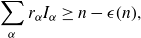 \begin{equation}\sum_\alpha r_\alpha I_\alpha \ge n - \epsilon(n),\end{equation}
for some set of non-negative weights $\{r_\alpha\}$
with
$\{r_\alpha\}$
with $\sum r_\alpha =1$
, and error term
$\sum r_\alpha =1$
, and error term $\epsilon(n)$
. Of course, we have
$\epsilon(n)$
. Of course, we have $\kappa(\tau)\ge I_\alpha$
for all
$\kappa(\tau)\ge I_\alpha$
for all $\alpha$
, and by convexity we must have
$\alpha$
, and by convexity we must have $I_\alpha \ge n-\epsilon(n)$
for some
$I_\alpha \ge n-\epsilon(n)$
for some $\alpha$
.
$\alpha$
.
We will rely on three facts from analytic number theory, which we group together in a single lemma for convenience. Below we indicate the interval $\{1,\ldots,m\}$
by [m] and the subset of
$\{1,\ldots,m\}$
by [m] and the subset of $\{1,\ldots,m\}$
relatively prime to s by
$\{1,\ldots,m\}$
relatively prime to s by $[m]_s$
, e.g.
$[m]_s$
, e.g. $\phi(m) = \#[m]_m$
. The number of divisors of n is indicated by d(n).
$\phi(m) = \#[m]_m$
. The number of divisors of n is indicated by d(n).
Table 1. Some data for attractive elements of $\mathcal{A}_n$
. Some entries include only leading-order terms, ignoring multiplicative constants. Note that
$\mathcal{A}_n$
. Some entries include only leading-order terms, ignoring multiplicative constants. Note that $\Phi = {1+\sqrt 5}/2$
.
$\Phi = {1+\sqrt 5}/2$
.
Lemma 4·1. We have the following estimates:
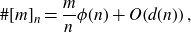 \begin{align} \#[m]_n & = \frac mn \phi(n) + O\!\left(d(n)\right), \end{align}
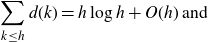 \begin{align} \sum_{k\le h} d(k)& = h \log h + O(h) \text{ and }\end{align}
 \begin{align} \sum_{k\le h} \frac {\phi(k)}k &= O(h).\end{align}
The estimate (4·2) is a standard application of Möbius inversion [Reference Cohen9, lemma 3·4]. The second estimate (4·3) is a weaker version of a famous theorem of Dirichlet [
Reference Apostol6
, chapter 3], and a more precise form of (4·4) can be found in [
Reference Walfisz30
]. (Note that the error term in (4·2) is in fact $O(\vartheta(n))$
, where
$O(\vartheta(n))$
, where $\vartheta(n)$
is the number of square-free divisors of n. However, in the sum
$\vartheta(n)$
is the number of square-free divisors of n. However, in the sum $\sum_{j\le h} \vartheta(j)$
, one finds the same order of growth as
$\sum_{j\le h} \vartheta(j)$
, one finds the same order of growth as $\sum_{j\le h} d(j)$
[
Reference Mertens21
], so in our application, Lemma 4·3, this improvement is immaterial.)
$\sum_{j\le h} d(j)$
[
Reference Mertens21
], so in our application, Lemma 4·3, this improvement is immaterial.)
In this section we will show:
Proposition 4·2. There is a constant $C>0$
so that, for any
$C>0$
so that, for any $\tau\in \mathcal{A}_n$
and any horoball H of
$\tau\in \mathcal{A}_n$
and any horoball H of $\tau$
with
$\tau$
with $h = \mathrm{ht}(\tau,H)$
, we have
$h = \mathrm{ht}(\tau,H)$
, we have $\kappa(\tau) \ge n - C h \log h$
.
$\kappa(\tau) \ge n - C h \log h$
.
As in Section 2·4, let $H_1$
and
$H_1$
and $H_2$
be the two horoballs that are incident to H along its two extreme edges. By construction, the non-backtracking path
$H_2$
be the two horoballs that are incident to H along its two extreme edges. By construction, the non-backtracking path $\sigma$
from
$\sigma$
from $H_1$
to
$H_1$
to $H_2$
is contained in H; we indicate the vertices
$H_2$
is contained in H; we indicate the vertices $\sigma$
passes through in order by
$\sigma$
passes through in order by $p_1,\ldots,p_w$
. See Figure 3.
$p_1,\ldots,p_w$
. See Figure 3.
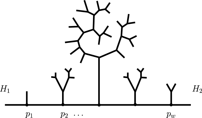
Fig. 3. The horoball H determines branches for $\tau$
, and extreme horoballs
$\tau$
, and extreme horoballs $H_1$
and
$H_1$
and $H_2$
.
$H_2$
.
For each j, the complement $\tau \setminus p_j$
consists of three components, and we indicate (the closure of) the unique such component that doesn’t intersect H as the jth branch B(j).
$\tau \setminus p_j$
consists of three components, and we indicate (the closure of) the unique such component that doesn’t intersect H as the jth branch B(j).
Label H with $1/0$
, label the horoball neighbouring H along the edge
$1/0$
, label the horoball neighbouring H along the edge $\overline{p_j p_{j+1}}$
with
$\overline{p_j p_{j+1}}$
with $0/1$
, and label the horoball neighbour of H along
$0/1$
, and label the horoball neighbour of H along $\overline{p_{j-1}p_j}$
with
$\overline{p_{j-1}p_j}$
with $1/1$
. Now Farey addition determines how to fill in labels for the remaining horoballs, and let
$1/1$
. Now Farey addition determines how to fill in labels for the remaining horoballs, and let $\mathrm{ht}_H \, B(j)$
indicate the maximum denominator among Farey labels for horoballs intersecting B(j).
$\mathrm{ht}_H \, B(j)$
indicate the maximum denominator among Farey labels for horoballs intersecting B(j).
We may count the n horoball regions of $\tau$
by filtering them according to their heights on the branches. That is, for each
$\tau$
by filtering them according to their heights on the branches. That is, for each $k\in \mathbb{N}$
, let
$k\in \mathbb{N}$
, let $X(k) = \{ j \;:\; \mathrm{ht}_H \, B(j) \ge k\}$
(that is, the set of indices j where the jth branch has height at least k), and let
$X(k) = \{ j \;:\; \mathrm{ht}_H \, B(j) \ge k\}$
(that is, the set of indices j where the jth branch has height at least k), and let $x_k = \#X(k)$
. See Figure 6.
$x_k = \#X(k)$
. See Figure 6.
Suppose that $k\le \mathrm{ht}_H\, B(j)$
. We now define ‘leftmost’ and ‘rightmost’ horoballs
$k\le \mathrm{ht}_H\, B(j)$
. We now define ‘leftmost’ and ‘rightmost’ horoballs $L(j)_k$
and
$L(j)_k$
and $R(j)_k$
at height at least k on the branch B(j), and corresponding ‘numerator invariants’
$R(j)_k$
at height at least k on the branch B(j), and corresponding ‘numerator invariants’ $\ell(j)_k$
and
$\ell(j)_k$
and $r(j)_k$
. Consider the subset of horoballs of B(j) whose relative heights to H are
$r(j)_k$
. Consider the subset of horoballs of B(j) whose relative heights to H are $\ge k$
, nonempty by assumption. We declare
$\ge k$
, nonempty by assumption. We declare $L(j)_k$
and
$L(j)_k$
and $R(j)_k$
to be the elements of this set with maximal and minimal Farey labels, respectively. (Among horoballs of B(j) at height
$R(j)_k$
to be the elements of this set with maximal and minimal Farey labels, respectively. (Among horoballs of B(j) at height $\ge k$
from H, the horoball
$\ge k$
from H, the horoball $L(j)_k$
appears furthest to the left from the viewpoint of H; similarly
$L(j)_k$
appears furthest to the left from the viewpoint of H; similarly $R(j)_k$
appears furthest to the right.) Now we define ‘numerator invariants’
$R(j)_k$
appears furthest to the right.) Now we define ‘numerator invariants’ $\ell(j)_k$
and
$\ell(j)_k$
and $r(j)_k$
for B(j) as follows: Suppose the Farey labels of
$r(j)_k$
for B(j) as follows: Suppose the Farey labels of $L(j)_k$
and
$L(j)_k$
and $R(j)_k$
are
$R(j)_k$
are $a_l/b_l$
and
$a_l/b_l$
and $a_r/b_r$
respectively. We let
$a_r/b_r$
respectively. We let $\ell(j)_k:=\lfloor k\cdot ({a_l}/{b_l}) \rfloor$
and
$\ell(j)_k:=\lfloor k\cdot ({a_l}/{b_l}) \rfloor$
and $r(j)_k:= \lceil k\cdot ({a_r}/{b_r}) \rceil$
. See Figure 4 and Figure 5.
$r(j)_k:= \lceil k\cdot ({a_r}/{b_r}) \rceil$
. See Figure 4 and Figure 5.
Consider $j_k^+$
(resp.
$j_k^+$
(resp. $j_k^-$
), the maximal (resp. minimal) index of X(k). Below, we indicate
$j_k^-$
), the maximal (resp. minimal) index of X(k). Below, we indicate $\lambda_k= \ell(j_k^-)_k$
and
$\lambda_k= \ell(j_k^-)_k$
and $\rho_k= r(j_k^+)_k$
; roughly speaking,
$\rho_k= r(j_k^+)_k$
; roughly speaking, $\lambda_k$
(resp.
$\lambda_k$
(resp. $\rho_k$
) is the ‘leftmost (resp. rightmost) height k numerator invariant’. See Figure 7.
$\rho_k$
) is the ‘leftmost (resp. rightmost) height k numerator invariant’. See Figure 7.
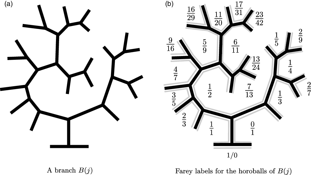
Fig. 4. A branch acquires Farey labels.
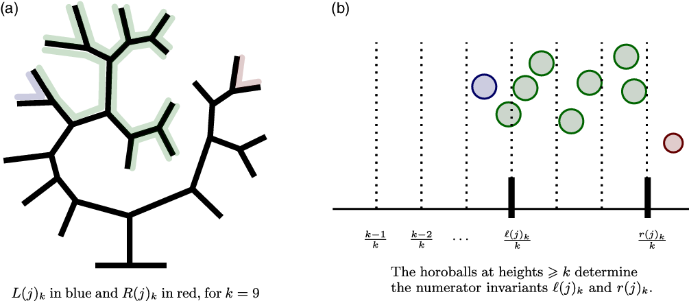
Fig. 5. The numerator invariants $\ell (j)_k$
and
$\ell (j)_k$
and $r(j)_k$
of B(j).
$r(j)_k$
of B(j).
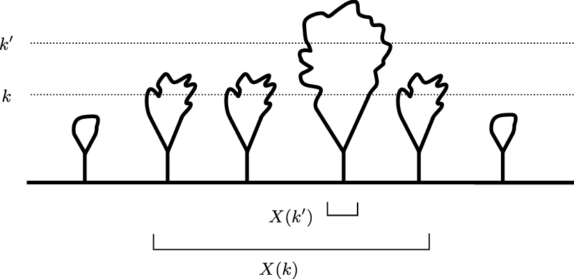
Fig. 6. The horoballs of $\tau$
may be filtered according to heights from H.
$\tau$
may be filtered according to heights from H.
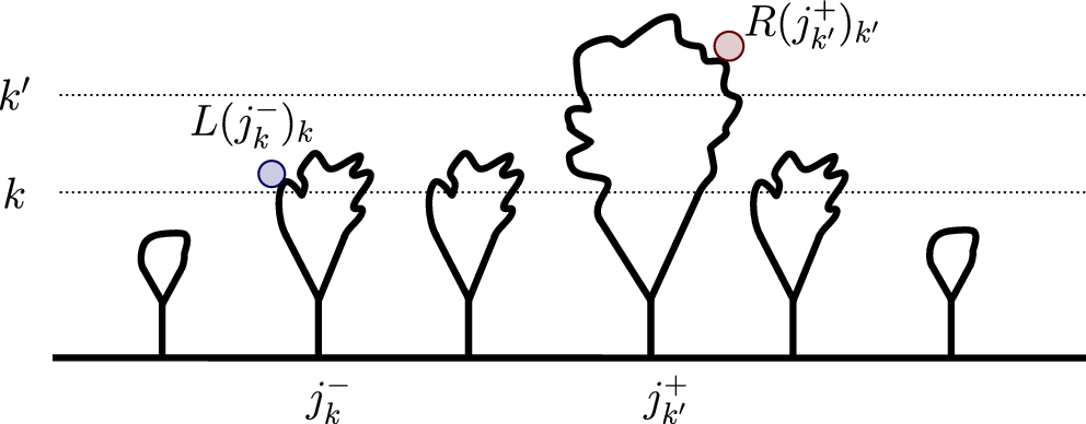
Fig. 7. The leftmost horoball at height $\ge k$
and rightmost horoball at height
$\ge k$
and rightmost horoball at height $\ge k'$
are used to build intersection number
$\ge k'$
are used to build intersection number $I_{kk^\prime}$
.
$I_{kk^\prime}$
.
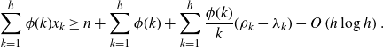
Lemma 4·3. We have
 \begin{equation*}\sum_{k=1}^h \phi(k)x_k \ge n + \sum_{k=1}^h \phi(k)+ \sum_{k=1}^h \frac{\phi(k)}k (\rho_k - \lambda_k)- O\left( h \log h\right).\end{equation*}
Proof. Observe that the sum of the number of horoballs of $\tau$
at height k relative to H, as k goes from 1 to h, is exactly
$\tau$
at height k relative to H, as k goes from 1 to h, is exactly $n-1$
.
$n-1$
.
The number of horoballs of B(j) at height k relative to H is at most $\phi(k)$
, so the total number of horoballs of
$\phi(k)$
, so the total number of horoballs of $\tau$
at height k from H is at most
$\tau$
at height k from H is at most $\phi(k) x_k$
. Observe that we may count the vertices of
$\phi(k) x_k$
. Observe that we may count the vertices of $B(j_k^-)$
and
$B(j_k^-)$
and $B(j_k^+)$
with slightly more care: Provided the numerators of horoballs of B(j) at height k are between
$B(j_k^+)$
with slightly more care: Provided the numerators of horoballs of B(j) at height k are between $\ell$
and r, the number of horoballs of B(j) at height k relative to H is at most
$\ell$
and r, the number of horoballs of B(j) at height k relative to H is at most $\phi(k)-\#[r-1]_k$
, and at most
$\phi(k)-\#[r-1]_k$
, and at most $\#[\ell]_k$
. Therefore the total number of horoballs of
$\#[\ell]_k$
. Therefore the total number of horoballs of $\tau$
at height k relative to H is at most
$\tau$
at height k relative to H is at most
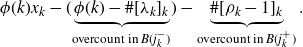 \begin{equation*}\phi(k)x_k - (\!\underbrace{\phi(k)-\#[\lambda_k]_k}_{\text{overcount in }B(j_k^-)}\!) - \underbrace{\#[\rho_k-1]_k}_{\text{overcount in }B(j_k^+)} .\end{equation*}
(The reader is reassured that the overcounts above are distinct when $j_k^-=j_k^+$
; in that case
$j_k^-=j_k^+$
; in that case $x_k=1$
and the expression simplifies to
$x_k=1$
and the expression simplifies to $\#[\lambda_k]_k - \#[\rho_k-1]_k$
.) By (4·2), the count above is at most
$\#[\lambda_k]_k - \#[\rho_k-1]_k$
.) By (4·2), the count above is at most
 \begin{equation*}\phi(k)x_k - \phi(k) + \frac{\lambda_k}k \phi(k) - \frac{\rho_k-1}k \phi(k) + O(d(k)).\end{equation*}
The sum of this expression as k goes from 1 to h is $n-1$
, so rearranging we find that
$n-1$
, so rearranging we find that
 \begin{equation*}\sum_{k=1}^h \phi(k)x_k \ge n +\sum_{k=1}^h \phi(k) + \sum_{k=1}^h \frac{\phi(k)}k (\rho_k-\lambda_k) - 1- \sum_{k=1}^h \frac{\phi(k)}k - C\sum_{k=1}^h d(k).\end{equation*}
By (4·3) and (4·4), the last three terms can be replaced by $O(h\log h)$
.
$O(h\log h)$
.
The reader may observe how Lemma 4·3 is somewhat suggestive of (4·1).
Given a choice of two heights k and k ′, consider the intersection number $I_{kk^\prime}$
between
$I_{kk^\prime}$
between $L(j_k^-)_k$
and
$L(j_k^-)_k$
and $R(j_{k^\prime}^+)_{k^\prime}$
. See Figure 7. It is straightforward to compute
$R(j_{k^\prime}^+)_{k^\prime}$
. See Figure 7. It is straightforward to compute
 \begin{equation*}I_{kk^\prime} \ge kk'|j_{k^\prime}^+ - j_k^-|+ k'\lambda_k - k \rho_{k^\prime}.\end{equation*}
Notice that $\big| j_{k^\prime}^+-j_k^-\big| + \big| j_{k}^+-j_{k^\prime}^-\big| \ge x_k+x_{k^\prime}-2$
, so upon dividing by kk ′ we find
$\big| j_{k^\prime}^+-j_k^-\big| + \big| j_{k}^+-j_{k^\prime}^-\big| \ge x_k+x_{k^\prime}-2$
, so upon dividing by kk ′ we find
 \begin{equation}\frac1{kk'} \left(I_{kk^\prime} + I_{k^\prime k}\right) \ge x_k+x_{k^\prime} - 2 + \left(\frac{\lambda_k}k- \frac{\rho_k}k\right) + \left(\frac{\lambda_{k^\prime}}{k'} - \frac{\rho_{k^\prime}}{k'}\right).\end{equation}
With Lemma 4·3 in mind, we would like to choose pairs $\{k,k'\}\subset [h]$
so that the sum over the choices made of the terms ‘
$\{k,k'\}\subset [h]$
so that the sum over the choices made of the terms ‘ $x_k+x_{k^\prime} $
’ on the right-hand side of (4·5) is equal to
$x_k+x_{k^\prime} $
’ on the right-hand side of (4·5) is equal to $\sum \phi(k)x_k$
; meanwhile, the sum of coefficients on the left-hand side should be equal to 1. The following proposition makes this idea feasible.
$\sum \phi(k)x_k$
; meanwhile, the sum of coefficients on the left-hand side should be equal to 1. The following proposition makes this idea feasible.
Proposition 4·4. For each $h\in \mathbb{N}$
, there is a graph
$h\in \mathbb{N}$
, there is a graph $\Gamma_h$
satisfying:
$\Gamma_h$
satisfying:
-
(i) the vertex set of
$\Gamma_h$
is given by
$\{1,\ldots, h\}$
; -
(ii) the valence of vertex k is
$\phi(k)$
; -
(iii) the sum
$\displaystyle \sum_{k\sim k^\prime} \frac2{kk'}$
over the edges of
$\Gamma_h$
is equal to 1.


See Figure 8 for a picture of $\Gamma_6$
.
$\Gamma_6$
.
Fig. 8. The graph $\Gamma_6$
as described in Proposition 4·4. Edge weights sum to 1.
$\Gamma_6$
as described in Proposition 4·4. Edge weights sum to 1.
Proof. Declare $k\sim k'$
when
$k\sim k'$
when $\gcd\!(k,k')=1$
and
$\gcd\!(k,k')=1$
and $k+k'>h$
.
$k+k'>h$
.
For property (ii), choose a vertex k. Each integer i relatively prime to k can be shifted by k to $i+k$
, another integer relatively prime to k. For
$i+k$
, another integer relatively prime to k. For $1\le i\le k$
, we may choose the maximum n so that
$1\le i\le k$
, we may choose the maximum n so that $i+nk\le h$
. The result is a bijection of
$i+nk\le h$
. The result is a bijection of $[k]_k$
, the integers in [k] relatively prime to k, with the set of integers k ′, relatively prime to k, less than h, and so that
$[k]_k$
, the integers in [k] relatively prime to k, with the set of integers k ′, relatively prime to k, less than h, and so that $k+k'>h$
. Therefore the valence of k is
$k+k'>h$
. Therefore the valence of k is $\#[k]_k=\phi(k)$
.
$\#[k]_k=\phi(k)$
.
For property (iii), observe that, to transform $\Gamma_h$
into
$\Gamma_h$
into $\Gamma_{h+1}$
, the edges
$\Gamma_{h+1}$
, the edges $k\sim k'$
with
$k\sim k'$
with $k+k'=h+1$
are deleted and replaced by edges
$k+k'=h+1$
are deleted and replaced by edges $k\sim(h+1)$
and
$k\sim(h+1)$
and $k'\sim(h+1)$
. Because
$k'\sim(h+1)$
. Because $k+k'=$
h+1, the edge weight
$k+k'=$
h+1, the edge weight $2/{kk'}$
in
$2/{kk'}$
in $\Gamma_h$
is equal to the sum of edge weights
$\Gamma_h$
is equal to the sum of edge weights $2/{k(h+1)}+2/{k'(h+1)}$
in
$2/{k(h+1)}+2/{k'(h+1)}$
in $\Gamma_{h+1}$
, so the sum
$\Gamma_{h+1}$
, so the sum $\sum_{k\sim k^\prime}2/{kk'}$
is independent of h. For the base case
$\sum_{k\sim k^\prime}2/{kk'}$
is independent of h. For the base case $h=2$
, observe that
$h=2$
, observe that $2/{1\cdot2}=1$
.
$2/{1\cdot2}=1$
.
Let E indicate the set of edges of $\Gamma_h$
. Now Proposition 4·4 and (4·5) imply:
$\Gamma_h$
. Now Proposition 4·4 and (4·5) imply:
 \begin{align*} \sum_{(k,k^\prime)\in E} \frac1{kk'} \left(I_{kk^\prime} + I_{k^\prime k}\right)& \ge \ \sum_{(k,k^\prime)\in E} \ \left[ x_k+x_{k^\prime} - 2 + \left(\frac{\lambda_k}k- \frac{\rho_k}k\right) + \left(\frac{\lambda_{k^\prime}}{k'} - \frac{\rho_{k^\prime}}{k'}\right) \right] \\&= \sum_k \phi(k) x_k \ -\ \sum_k \phi(k) \ + \ \sum_k \frac{\phi(k)}k \left( \lambda_k - \rho_k \right)\end{align*}
Applying Lemma 4·3, we find that
 \begin{equation}\sum_{(k,k^\prime)\in E} \frac1{kk'} \left(I_{kk^\prime} + I_{k^\prime k}\right) \ge n - O\!\left( h \log h\right).\end{equation}
Because $\sum_E 2/{kk'} =1$
by Proposition 4·4, the left-hand side of (4·6) is a convex combination of intersection numbers for
$\sum_E 2/{kk'} =1$
by Proposition 4·4, the left-hand side of (4·6) is a convex combination of intersection numbers for $\tau$
. Therefore inequality (4·6) implies that there is a pair of horoballs whose intersection number is at least the right-hand side, proving Proposition 4·2.
$\tau$
. Therefore inequality (4·6) implies that there is a pair of horoballs whose intersection number is at least the right-hand side, proving Proposition 4·2.
5. Finding a horoball of controlled relative height
For many $\tau\in\mathcal{A}_n$
, there exist H so that the
$\tau\in\mathcal{A}_n$
, there exist H so that the $\mathrm{ht}(\tau,H)$
is O(1), so Proposition 4·2 with height demonstrates that
$\mathrm{ht}(\tau,H)$
is O(1), so Proposition 4·2 with height demonstrates that $\kappa(\tau)=n-O(1)$
. However, such a horoball need not exist, e.g. every horoball of
$\kappa(\tau)=n-O(1)$
. However, such a horoball need not exist, e.g. every horoball of $\mathrm{ach}(n)$
has height at least
$\mathrm{ach}(n)$
has height at least $\approx (({1+\sqrt 5})/2)^{n/2}$
. Nonetheless,
$\approx (({1+\sqrt 5})/2)^{n/2}$
. Nonetheless, $\kappa(\mathrm{ach}(n))$
is quite large (on the order
$\kappa(\mathrm{ach}(n))$
is quite large (on the order $({1+\sqrt 5})/2)^n$
), so one might hope that it is always possible to find horoballs of small height relative to
$({1+\sqrt 5})/2)^n$
), so one might hope that it is always possible to find horoballs of small height relative to $\kappa(\tau)$
. We show:
$\kappa(\tau)$
. We show:
Proposition 5·1. There exists a constant $C>0$
so that, for any
$C>0$
so that, for any $\tau\in \mathcal{A}_n$
, there exists a horoball H of
$\tau\in \mathcal{A}_n$
, there exists a horoball H of $\tau$
so that the height of
$\tau$
so that the height of $\tau$
relative to H is controlled as
$\tau$
relative to H is controlled as $\mathrm{ht}(\tau,H) \le C \sqrt{\kappa(\tau)}$
.
$\mathrm{ht}(\tau,H) \le C \sqrt{\kappa(\tau)}$
.
Remark. The reader can observe that the conclusion above fits the data in Table 1. It is tempting to hope for an improvement of Proposition 5·1 along the following lines: as $\kappa(\tau)$
gets closer to
$\kappa(\tau)$
gets closer to $\min \kappa$
(e.g. if
$\min \kappa$
(e.g. if $\kappa(\tau)\le n$
), one should be able to find horoballs of
$\kappa(\tau)\le n$
), one should be able to find horoballs of $\tau$
with relative heights
$\tau$
with relative heights $\ll \sqrt n$
.
$\ll \sqrt n$
.
On the other hand, the row containing $\tau=\mathrm{Far}(h)$
, with
$\tau=\mathrm{Far}(h)$
, with $n\approx 3/{\pi^2}h^2$
, makes this hope seem quite remote. Indeed,
$n\approx 3/{\pi^2}h^2$
, makes this hope seem quite remote. Indeed, $\kappa(\mathrm{Far}(h))$
is greater than n only by the innocuous looking linear factor
$\kappa(\mathrm{Far}(h))$
is greater than n only by the innocuous looking linear factor $\frac {\pi^2}3 \approx 3.3$
, yet every horoball has relative height
$\frac {\pi^2}3 \approx 3.3$
, yet every horoball has relative height $\ge h \approx \sqrt n$
.
$\ge h \approx \sqrt n$
.
Proof. Let $K_1,K_2$
be horoballs of
$K_1,K_2$
be horoballs of $\tau$
so that
$\tau$
so that $\iota(K_1,K_2)=\kappa(\tau)$
, and let
$\iota(K_1,K_2)=\kappa(\tau)$
, and let $r=\log \kappa(\tau)$
. By Lemma 2·3, we have
$r=\log \kappa(\tau)$
. By Lemma 2·3, we have $d_{\mathbb{H}^2}(K_1,K_2) = 2r$
.
$d_{\mathbb{H}^2}(K_1,K_2) = 2r$
.
Let $x\in \mathbb{H}^2$
be the midpoint of the geodesic from
$x\in \mathbb{H}^2$
be the midpoint of the geodesic from $K_1$
to
$K_1$
to $K_2$
. By Lemma 2·2 there is a horoball
$K_2$
. By Lemma 2·2 there is a horoball $H\in\mathcal{H}$
so that
$H\in\mathcal{H}$
so that $d_{\mathbb{H}^2}(H,x)\le \log (2/{\sqrt3})$
. The horoball H corresponds to a horoball in the dual tree to
$d_{\mathbb{H}^2}(H,x)\le \log (2/{\sqrt3})$
. The horoball H corresponds to a horoball in the dual tree to $\mathcal{F}$
which is, by construction, incident to the geodesic between
$\mathcal{F}$
which is, by construction, incident to the geodesic between $K_1$
and
$K_1$
and $K_2$
. By Lemma 2·4, H is a horoball in
$K_2$
. By Lemma 2·4, H is a horoball in $\tau$
as well. (Strictly speaking, one could distinguish notationally between Farey horoballs in
$\tau$
as well. (Strictly speaking, one could distinguish notationally between Farey horoballs in $\mathcal{H}$
, horoballs in the dual tree to
$\mathcal{H}$
, horoballs in the dual tree to $\mathcal{F}$
, and horoballs in
$\mathcal{F}$
, and horoballs in $\tau$
; because we feel it only obscures the relevant choices, we leave this distinction to be implied by the reader.)
$\tau$
; because we feel it only obscures the relevant choices, we leave this distinction to be implied by the reader.)
We claim that H satisfies the requisite bound. Let K be any other horoball of $\tau$
. Because
$\tau$
. Because $\mathbb{H}^2$
is
$\mathbb{H}^2$
is $\delta$
-hyperbolic, the point x is within
$\delta$
-hyperbolic, the point x is within $\delta$
of the geodesic segment between K and
$\delta$
of the geodesic segment between K and $K_i$
for i equal to either 1 or 2. A standard application of the triangle inequality (see Figure 9) then yields
$K_i$
for i equal to either 1 or 2. A standard application of the triangle inequality (see Figure 9) then yields
 \begin{equation*}d_{\mathbb{H}^2}(K,K_i) \ge d_{\mathbb{H}^2}(K,x) + d_{\mathbb{H}^2}(x,K_i) - 2\delta = d_{\mathbb{H}^2}(K,x) + r -2\delta.\end{equation*}
Because $d_{\mathbb{H}^2}(K,K_i)\le 2r$
, we conclude that
$d_{\mathbb{H}^2}(K,K_i)\le 2r$
, we conclude that $d_{\mathbb{H}^2}(K,x)\le r+2\delta$
, and
$d_{\mathbb{H}^2}(K,x)\le r+2\delta$
, and
 \begin{equation*}d_{\mathbb{H}^2}(H,K)\le d_{\mathbb{H}^2}(H,x) + d_{\mathbb{H}^2}(x,K) \le \log \frac2{\sqrt 3}+ r +2\delta.\end{equation*}
By Lemma 2·3 we conclude that
 \begin{equation*}\iota(H,K) = e^{\frac12 d_{\mathbb{H}^2}(H,K) }\le \frac2{\sqrt 3}e^{2\delta} \sqrt{\kappa(\tau)}.\end{equation*}
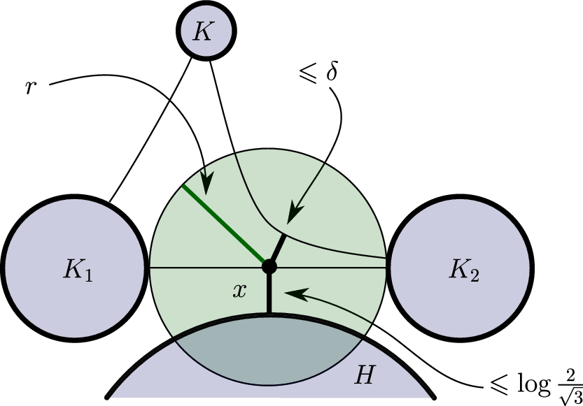
Fig. 9. A horoball K not far from the $K_i$
is not far from H as well.
$K_i$
is not far from H as well.
Remark. Ian Agol has suggested a slightly different version of the above proof: choose Farey labels for the horoballs in $\tau$
, and enlarge the horoballs by
$\tau$
, and enlarge the horoballs by $\log \kappa(\tau)+\log (2/{\sqrt3})$
. A variation on Lemma 2·2 together with Lemma 2·3 implies that every trio of these horoballs mutually intersect, so by Helly’s theorem there is a point x in their common intersection [
Reference Helly19
], and one may finish as above.
$\log \kappa(\tau)+\log (2/{\sqrt3})$
. A variation on Lemma 2·2 together with Lemma 2·3 implies that every trio of these horoballs mutually intersect, so by Helly’s theorem there is a point x in their common intersection [
Reference Helly19
], and one may finish as above.
6. From kappa to eta
As stated in the introduction, it is an exercise to show that
 \begin{equation*}\eta_T(k) = \max \{ n\;:\; \kappa_T(n)\le k\}.\end{equation*}
By Theorem 1·2, we may conclude $\eta_T(k)\le \max\{n\;:\; n-C\sqrt n\log n \le k\}$
.
$\eta_T(k)\le \max\{n\;:\; n-C\sqrt n\log n \le k\}$
.
Theorem 1·1 now follows from the following lemma:
Lemma 6·1. Suppose that $C>0$
is a constant, and that
$C>0$
is a constant, and that $f\;:\;\mathbb{R}\to\mathbb{R}$
is an increasing, sublinear function, with
$f\;:\;\mathbb{R}\to\mathbb{R}$
is an increasing, sublinear function, with $f(x)=o(x)$
. There is a
$f(x)=o(x)$
. There is a $D>0$
so that for any
$D>0$
so that for any $k\ge 1$
we have
$k\ge 1$
we have $\max\{ x\;:\; x- Cf(x)\le k\} \le k+ D f(k)$
.
$\max\{ x\;:\; x- Cf(x)\le k\} \le k+ D f(k)$
.
Proof. Because $f(x)=o(x)$
, there is a
$f(x)=o(x)$
, there is a $C_1>0$
large enough so that
$C_1>0$
large enough so that $C_1-1>Cf(C_1)$
. Because f is sublinear, for any
$C_1-1>Cf(C_1)$
. Because f is sublinear, for any $k\ge 1$
we have
$k\ge 1$
we have
 \begin{equation*}(C_1-1)k > Ck \, f(C_1) \ge C f(C_1k).\end{equation*}
Adding k to both sides and rearranging we find
 \begin{equation}C_1k-C f(C_1k) > k.\end{equation}
Let $F(k)=\max\{ x\;:\; x-Cf(x)\le k\}$
. By (6·1) we have
$F(k)=\max\{ x\;:\; x-Cf(x)\le k\}$
. By (6·1) we have $F(k) < C_1k$
. Of course, by definition of F(k) we have
$F(k) < C_1k$
. Of course, by definition of F(k) we have $F(k) - Cf(F(k)) \le k$
. Because f is increasing and sublinear, we find
$F(k) - Cf(F(k)) \le k$
. Because f is increasing and sublinear, we find
 \begin{equation*}F(k) \le k+C f(F(k)) \le k+C f(C_1k) \le k+CC_1 f(k),\end{equation*}
as claimed.
Because $\sqrt x\log x$
is increasing and sublinear, this completes the proof of Theorem 1·1.
$\sqrt x\log x$
is increasing and sublinear, this completes the proof of Theorem 1·1.
Remark. The conclusion of Lemma 6·1 holds under much weaker assumptions. For instance, sublinearity of f can be replaced by the assumption that there is some $C_2>0$
so that
$C_2>0$
so that $f(x+y) $
is at most
$f(x+y) $
is at most $C_2 f(x) + C_2 f(y)$
.
$C_2 f(x) + C_2 f(y)$
.
Acknowledgements
The authors thank Josh Greene and Ian Agol for valuable feedback on an early draft of this paper, and an anonymous referee for their fastidious reading. We are especially grateful to Ian Agol for sharing with us an unpublished note that contained Lemma 2·4, and for suggesting an alternative to our proof of Proposition 5·1 (see Figure 5).


 Open access