


1. Introduction
Macroeconomics is traditionally divided into two main research areas: business cycles and long-run growth. This distinction, although useful for practical purposes, is artificial and assumes away any connection between fluctuations in economic activity and its trend. Yet, the disappointing performance of the US economy in the aftermath of the Great Recession generated a widespread belief that the two phenomena are connected.
Economists have not overlooked this topic entirely. According to endogenous growth theory, the growth rate of aggregate productivity is a function of the level of R&D investment. This proposition is particularly relevant given the well-documented pro-cyclicality of R&D investment. Therefore, if a shock displaces output from its trend and similarly affects the R&D level, the aggregate productivity growth rate will also be impacted. If this change in aggregate productivity growth is not compensated later by an equal change in the opposite direction, the productivity level is permanently changed, a phenomenon known as hysteresis.Footnote 1
Economists credit Schumpeter (Reference Schumpeter1942) as the first scholar to discuss how fluctuations in demand could affect the rate of innovation and, thus, long-term output growth, a view that is formally and concisely illustrated in Aghion and Saint-Paul (Reference Aghion and Saint-Paul1998). He theorized a counter-cyclicality of R&D spending due to the decreased opportunity cost of reallocating resources from production to R&D during the recessionary periods. During recessions, low demand implies a low marginal profitability of production, thus increasing the attractiveness of devoting those resources to R&D. The subsequent realization that in the data R&D is instead pro-cyclical promoted a noteworthy effort to produce alternative theories. The result is a long list of influential papers that propose various explanations for the persistence of cyclical fluctuations or hysteresis through this channel (Shleifer, Reference Shleifer1986; Fatas, Reference Fatas2000; Comin and Gertler, Reference Comin and Gertler2006; Barlevy, Reference Barlevy2007; Francois and Lloyd-Ellis, Reference Francois and Lloyd-Ellis2009; Nuño, Reference Nuño2011; Aghion et al. Reference Aghion, Askenazy, Berman, Cette and Eymard2012; Fatás and Summers, Reference Fatás and Summers2018; Bianchi et al. Reference Bianchi, Kung and Morales2019; Mand, Reference Mand2019; Queralto, Reference Queralto2020; Anzoategui et al. Reference Anzoategui, Comin, Gertler and Martinez2019).
On the empirical side, the magnitude and the shape of the response of R&D to shocks that cause the business cycle are unknown. Therefore, our main question is whether the response of R&D and productivity to a business cycle shock is consistent with theoretical predictions and quantitatively sizeable. Next, because different models propose different explanations for R&D’s pro-cyclicality that imply different behaviors of R&D to other macroeconomic shocks, our supplementary goal is to rule out some of these explanations as the main cause of R&D’s pro-cyclicality.
This paper achieves these goals by computing impulse response functions for R&D and aggregate productivity to shocks that caused the US business cycle in the post-WWII period. We employ a structural VAR to test the theoretical predictions and assess their quantitative relevance. In our main specification, the VAR includes three variables: R&D spending, utilization-adjusted total factor productivity (TFP), and cyclical unemployment. We impose a recursive structure with short-run restrictions. Specifically, utilization-adjusted TFP does not respond on impact to changes in R&D and unemployment, and unemployment does not react on impact to changes in R&D. We use the forecast error of the cyclical unemployment time series as a proxy for shocks that cause a deviation of output from its trend, justified by recent evidence (Angeletos et al. Reference Angeletos, Collard and Dellas2020). Responses to an exogenous increase in TFP, instead, help us in answering our supplementary question, assessing the validity of different theories on R&D’s cyclicality.
Our results provide evidence of hysteresis through the mechanism described in endogenous growth theory. The pattern of R&D and TFP following an exogenous increase in cyclical unemployment is consistent with the theoretical predictions. Namely, R&D spending responds pro-cyclically. Moreover, TFP decreases gradually before stabilizing at a permanently lower trend. This effect is substantial: when cyclical unemployment rises by 1 percentage point above its sample average, R&D growth remains significantly below trend for nearly two years, leading to a permanent TFP loss of approximately 1.3%. The reason this effect is so large is because the shock identified by the VAR is very persistent. Hence, persistent deviations of TFP growth from its trend add up to a large level effect, even though a small share of changes in TFP growth is explained by the business cycle shock, confirming a standard result in the literature (see, e.g., Angeletos et al. Reference Angeletos, Collard and Dellas2020). To better understand the magnitude of this effect we show the historical variance decomposition, which illustrates three main instances where the hysteresis effect is noteworthy: the 1960s boom, about 7.5% gain in TFP from the mid-1960s to the mid-1970s; the Volcker disinflation period, about 5% foregone TFP from the early to mid-1980s; and the Great Recession, about 6% foregone TFP from the start of the Great Recession to 2015, in line with estimates from Anzoategui et al. (Reference Anzoategui, Comin, Gertler and Martinez2019). The effect in all other periods is relatively small.
Notably, our empirical findings support aspects of Schumpeter’s original hypothesis regarding the counter-cyclicality of R&D. Following a positive exogenous increase in TFP, R&D declines. This result answers our supplementary question, as it allows us to rule out some explanations for the pro-cyclicality of R&D. Models attributing R&D’s pro-cyclicality to physical capital in R&D technology or to expected profit cycles generally predict an increase in R&D after a TFP shock. Instead, theories that emphasize credit constraints as the element responsible for R&D’s pro-cyclicality, such as Aghion et al. (Reference Aghion, Askenazy, Berman, Cette and Eymard2012), are in line with our findings. They predict counter-cyclical R&D in case of a TFP shock, and pro-cyclical R&D in the case of other shocks that affect firms’ access to liquidity. New Keynesian models incorporating nominal rigidities (Anzoategui et al. Reference Anzoategui, Comin, Gertler and Martinez2019; Aysun, Reference Aysun2020) also align with our findings, suggesting that a positive TFP shock can temporarily reduce both employment and R&D.
Empirical work on the connection between business cycle and long-run growth abounds. Cerra et al. (Reference Cerra, Fatás and Saxena2023) provide a comprehensive literature review going back to the early 1980s. While early work is concerned with employing statistical techniques to separate trends and deviations, some more recent work is closer to our analysis as it focuses more heavily on specific transmission mechanisms. Some of it studies single events, typically financial and banking crises, see, for example, Cerra and Saxena (Reference Cerra and Saxena2008). On the mechanism that we consider, notable examples include Aghion et al. (Reference Aghion, Askenazy, Berman, Cette and Eymard2012), Ouyang (Reference Ouyang2011), Kabukcuoglu (Reference Kabukcuoglu2019), and Duval et al. (Reference Duval, Hong and Timmer2020). All these studies analyze firm-level data. Their general theme is that firms hit by a negative shock reduce more strongly their innovation effort when their balance sheet is weak or when their financing opportunities are limited.
In general, the idea that temporary negative shocks can cause persistent, or even permanent, output losses relative to pre-shock trend is already corroborated by empirical evidence. The idea that one of the transmission channels could be R&D is backed by evidence too. What remains uncertain is the size of this effect, which may vary from country to country, the shape of impulse response functions for aggregate variables, and the reason why R&D evolves pro-cyclically.
Specifically, three important gaps remain. First, there is limited empirical evidence quantifying the long-run impact of cyclical shocks on aggregate productivity through the R&D channel. Second, existing studies often focus on single episodes or rely on calibrated dynamic stochastic general equilibrium (DSGE) models. Instead, we adopt a structural vector autoregression (SVAR) approach. Third, while theoretical models propose different mechanisms for R&D’s pro-cyclicality, there is little consensus on which of these are the most relevant at the aggregate level. Our paper addresses all three gaps.
This paper contributes to the literature by providing the first SVAR-based evidence of hysteresis operating through the R&D channel in the post-WWII U.S. data. While prior studies have explored the pro-cyclicality of R&D at the firm or industry level (e.g., Aghion et al. Reference Aghion, Askenazy, Berman, Cette and Eymard2012; Duval et al. Reference Duval, Hong and Timmer2020), and others have analyzed the long-run impact of individual shocks such as the Great Recession (e.g., Anzoategui et al. Reference Anzoategui, Comin, Gertler and Martinez2019), we take a broader empirical approach by analyzing the whole period through the lens of endogenous growth theory. Our framework enables us to quantify the long-run productivity impact of business cycle shocks and assess their historical significance. In doing so, we also provide new empirical tests to distinguish between competing theoretical explanations for R&D’s pro-cyclicality.
The paper is organized as follows. Section 2 illustrates the theory, Section 3 discusses the data, Section 4 introduces the empirical approach, Section 5 shows the results, Section 6 illustrates robustness tests, and Section 7 concludes.
2. From short-run shocks to permanent productivity changes: an illustration of the theory
This section presents the relevant features of the theory that we test. In outlining the theory, we focus on elements pertinent to our empirical purposes, namely, the production and investment side of the economy. We only mention the theoretical ingredients responsible for driving the R&D cyclical behavior we investigate.
The effects of pro-cyclical R&D
For decades, economists have been focusing on R&D to understand long-run growth. Endogenous growth theory is an outcome of their efforts. Early endogenous growth models, like Romer (Reference Romer1990), rely on the aggregate production function:
 \begin{equation} Y_t = f(A_t,L_t), \end{equation}
where $A$
denotes technological knowledge, and
$A$
denotes technological knowledge, and $L$
is labor. The production function is increasing in its inputs.
$L$
is labor. The production function is increasing in its inputs.
The critical feature of endogenous growth theory is the R&D technology. The most straightforward specification in discrete time is the following:
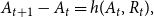 \begin{equation} A_{t+1}-A_t= h(A_t, R_t), \end{equation}
where $R_t$
is an endogenous variable that denotes R&D effort, which in this specification consists of labor from scientists and engineers. The R&D technology is assumed to be separable, increasing in its inputs, and linear in
$R_t$
is an endogenous variable that denotes R&D effort, which in this specification consists of labor from scientists and engineers. The R&D technology is assumed to be separable, increasing in its inputs, and linear in $A_t$
. The linear dependence of technological knowledge on the existing stock of knowledge drives endogenous growth. Given these assumptions, we can re-express the equation as follows by dividing both sides by
$A_t$
. The linear dependence of technological knowledge on the existing stock of knowledge drives endogenous growth. Given these assumptions, we can re-express the equation as follows by dividing both sides by $A_t$
:
$A_t$
:
 \begin{equation} g^{A}_{t+1}=h(R_t). \end{equation}
In other words, the rate of technological knowledge growth depends on the level of R&D investment.Footnote
2
In the absence of population growth (or after introducing elements that sterilize the scale effect), the theory predicts a stationary $R_t$
, thus leading to constant technological knowledge growth that depends on an endogenous variable.
$R_t$
, thus leading to constant technological knowledge growth that depends on an endogenous variable.
Words of caution are needed when analyzing the relationship between these aggregate variables. Endogenous growth theory has made progress ever since the original Romer’s contribution. Specifically, other variables stand in the way of aggregate R&D in determining the path of aggregate productivity growth. Some examples include the average firm size (Peretto and Connolly, Reference Peretto and Connolly2007), the degree of industry concentration (Ghazi, Reference Ghazi2019), government R&D spending (Huang et al. Reference Huang, Lai and Peretto2025), and entry/exit and churning within the firm size distribution (Massari, Reference Massari2023). Some factors, like government R&D spending, are irrelevant in business cycle analysis since they do not exhibit cyclical behavior. Other factors vary along the business cycle. In particular, available empirical evidence favors endogenous growth models that link productivity growth to average R&D expenditure, that is, R&D divided by the number of firms, thus taking into account average firm size.Footnote 3 We nevertheless decide to exclude them for three main reasons.
First, data availability is a limitation, as variables like the number of firms are only available annually from the late 1970s onward. As one of our goals is to understand whether hysteresis is present and quantitatively important, we believe that the better way to proceed involves exploiting the whole sample of R&D and TFP and the highest frequency of data that is available, which for this variable is quarterly.
Second, another goal is to understand whether R&D and productivity’s comovement in response to shocks that cause the business cycle is consistent with theoretical predictions, which concern the behavior of aggregate variables. There is room for introducing additional features to these models, but we believe that it is the responsibility of theory to point out how additional elements that affect the R&D technology play a role in reinforcing, weakening, or preventing hysteresis. An interpretation of the existing literature is that, while accounting for the dynamics of average firm size is important in understanding long-run growth, scholars in this literature do not currently believe that changes in the average firm size at business cycle frequency are an important driver of productivity growth dynamics in the short or medium run.
Third, as we will describe later, we do not impose equation (3) in our empirical analysis. We use it as a guideline for selecting variables and imposing restrictions that remain valid across different specifications of the productivity-R&D relationship. Instead, our empirical approach permits deviations from a strictly positive relationship between R&D and productivity growth. Thus, it is a test of the most basic model of endogenous growth subject to business cycle shocks.
Finally, various theoretical models predict a pro-cyclical response of R&D effort following a business cycle shock. Because different models explore different mechanisms for R&D’s pro-cyclicality, we postpone the illustration of this aspect of the theory to the next subsection. Meanwhile, we focus on the common implication of these models that is related to our main question, namely, the hysteresis effects of business cycle shocks when R&D effort is endogenous and pro-cyclical.
Figure 1 displays the predicted responses of four key variables to a negative business cycle shock, as suggested by the theoretical model. Cyclical unemployment, which we use as the variable of reference for the business cycle, increases. Because the theory predicts that R&D effort is pro-cyclical, it decreases as the shock appears and then reverts to its original level. Because the dynamics of productivity are governed by equation (3), the productivity growth rate (not shown) follows the same path as R&D, although with a one-period lag. Meanwhile, the productivity level, which is the sum of the log deviations of productivity growth from its steady-state value, gradually moves from its pre-shock trend, before stabilizing on a parallel and permanently lower the new trend. That is, the temporary loss in the flow of new ideas determines a permanent loss in the stock of ideas. Finally, we show the behavior of R&D spending. The reason we show both R&D effort and spending is that whereas R&D effort is the relevant variable to understand the theoretical model, R&D spending is the observable variable at the frequency that our empirical exercise requires. Notice that, while R&D effort reverts to its pre-shock trend, R&D spending does not. R&D spending is permanently affected because wages paid to R&D personnel reflect the behavior of productivity. However, the steady-state amount of resources devoted to R&D is unchanged, ensuring that the productivity growth rate reverts to its pre-shock level after the shock has fully propagated.
The impulse responses presented in Figure 1 are the theoretical predictions that we test to answer the main question of this paper.
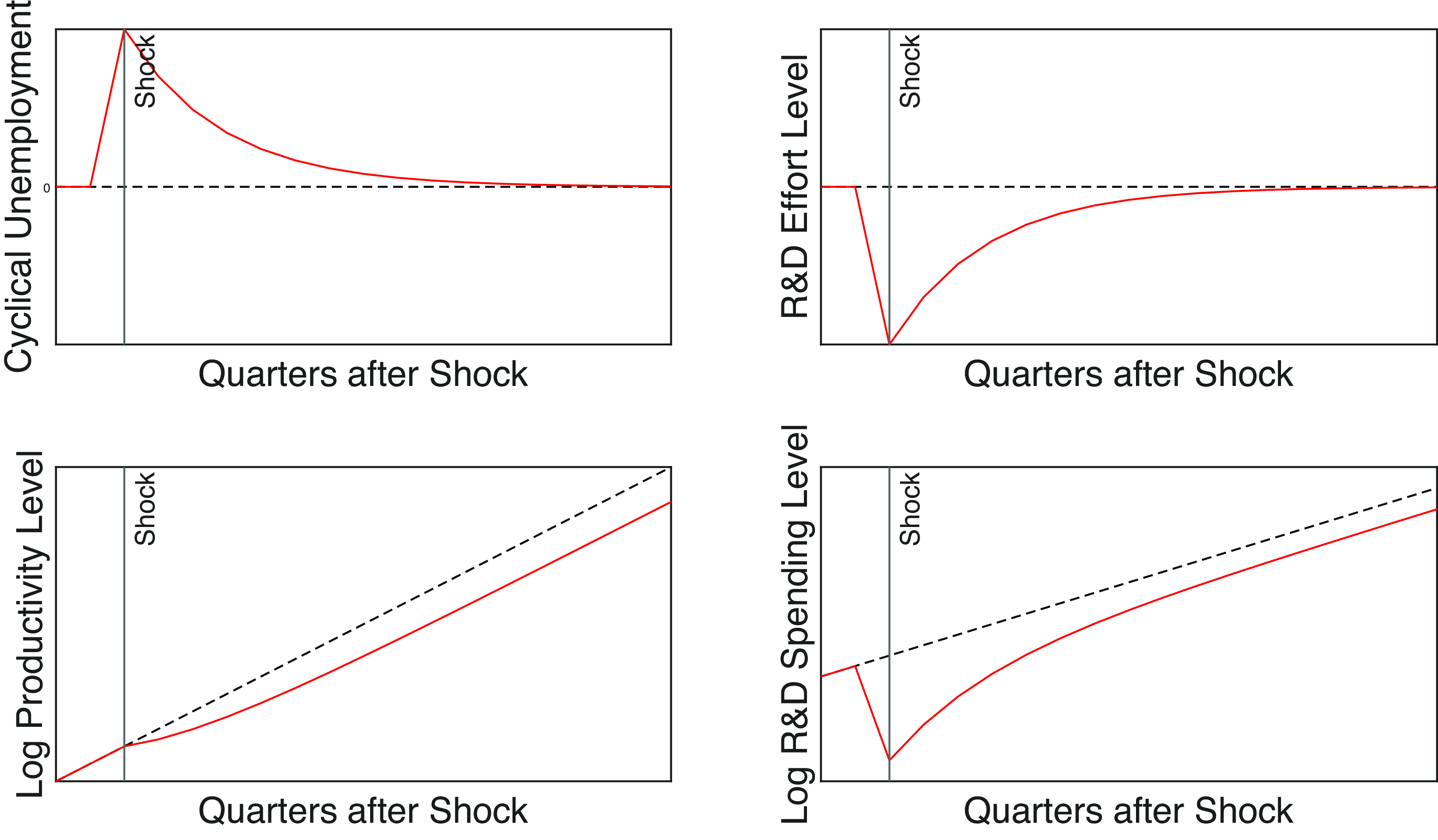
Figure 1. Theoretical predictions following a negative shock.Note: Impulse responses to a shock that increases the cyclical unemployment rate. R&D is assumed pro-cyclical, while productivity moves according to the equations illustrated. The black line is the pre-shock trend.
Why is R&D pro-cyclical?
As R&D is an endogenous variable, what does the theory predict regarding its behavior over the business cycle? Schumpeter (Reference Schumpeter1942) is credited as the first economist to analyze R&D within the context of business cycles. In his view, R&D moves counter-cyclically because the opportunity cost of allocating resources to R&D increases during booms, when production is particularly profitable. As data became available, after noticing that aggregate R&D spending and employment correlate positively with output, economists rejected this explanation and theorized different mechanisms to explain this pro-cyclicality.
Currently, multiple explanations coexist in the literature. Some theories still attribute R&D’s cyclical behavior to the pro-cyclicality of profits. However, they add some features to ensure that R&D is pro-cyclical. For example, Barlevy (Reference Barlevy2007) assumes that imitation leads to the dissipation of profits derived from R&D after some time. Therefore, firms become short-term oriented and invest in R&D when profitability increases, which happens during booms. Francois and Lloyd-Ellis (Reference Francois and Lloyd-Ellis2009), picking up insights from Shleifer (Reference Shleifer1986), introduce lags between R&D, commercialization, and implementation of the innovation. As firms would find it profitable to implement the innovation during business cycle peaks, efforts in commercialization will be stronger in worse times, and R&D activities will precede them, thus tending to coincide with booms.
Other explanations rely on the idea that R&D does not consist exclusively of spending on scientists and engineers. Comin and Gertler (Reference Comin and Gertler2006) model R&D as lab equipment, while Mand (Reference Mand2019) emphasizes the complementarity between scientists, engineers, physical capital, and support staff. The greater availability of capital goods during booms facilitates R&D investment.
An additional explanation relies on the inclusion of financial frictions. By assuming that firms rely on credit to finance R&D, shocks that tighten financial conditions limit their possibility to conduct this type of investment. To the extent that credit availability is pro-cyclical, and if this force is stronger than the forces that drive counter-cyclical R&D, these models predict pro-cyclical R&D. Examples of this explanation include Aghion et al. (Reference Aghion, Askenazy, Berman, Cette and Eymard2012), Queralto (Reference Queralto2020), and Bianchi et al. (Reference Bianchi, Kung and Morales2019).
Finally, Anzoategui et al. (Reference Anzoategui, Comin, Gertler and Martinez2019) and Aysun (Reference Aysun2020) propose a endogenous growth models with New Keynesian features. Anzoategui et al. (Reference Anzoategui, Comin, Gertler and Martinez2019) combine the pro-cyclicality of profits with stickiness in R&D personnel’s wages. As a result, the cost of conducting R&D responds with some lag to shocks that cause the business cycle. Instead, Aysun (Reference Aysun2020) builds a model with labor-intensive R&D and diminishing returns to labor in production. Therefore, shocks that lead to higher equilibrium employment would lead to higher production employment. Due to diminishing returns to production labor, R&D employment would also rise to balance out marginal products. Instead, following a productivity shock, the model can deliver counter-cyclical R&D if labor hours or employment move in the opposite direction as productivity. The theory allows for this possibility in models with nominal rigidities or in models with particularly strong income effects (Basu et al. Reference Basu, Fernald and Kimball2006).
3. Data
The analysis relies on US quarterly data for R&D, TFP, and unemployment. The period under consideration starts in quarter 1 of 1949 and ends in quarter 4 of 2019.
The data series for R&D is the real and seasonally adjusted gross private domestic investment in intellectual property products from the National Income and Product Accounts (Bureau of Economic Analysis). We focus on private R&D, as theory suggests that market effects drive its response to cyclical shocks. We tried adding public R&D spending to the analysis as an additional variable, concluding that it does not add anything of interest. Next, to ensure that the cyclicality of R&D results from changes in resources devoted to it and not to its price, we focus on a measure of workers’ salaries with a bachelor’s degree, which exists at a quarterly frequency starting from 2000. At an annual frequency, it dates back to 1979. Since high-skilled worker salaries exhibit minimal cyclicality, they are unlikely to be the primary driver of R&D fluctuations.
When considering productivity, we rely on Fernald’s series on utilization-adjusted TFP (Fernald, Reference Fernald2014), which removes variations in productivity due to changes in labor effort and capital usage. We use the utilization-adjusted measure as it better captures long-run productivity trends. Removing the utilization of other factors of production provides us with a better estimate of the product of R&D. Utilization-adjusted TFP serves as the best proxy for the stock of productive ideas. In addition to these considerations, it is worth noting that the reliance on this modified TFP measure is the TFP shock identification strategy adopted in Basu et al. (Reference Basu, Fernald and Kimball2006). In that paper, innovations to this time series are interpreted as TFP shocks. Our paper follows the same route while adding the short-run restrictions introduced in the next section.
To better isolate changes in the stock of technological knowledge, we apply a four-period moving average to the TFP time series. We follow Comin and Gertler (Reference Comin and Gertler2006) rationale in removing the higher frequency component in the TFP time series to isolate what they define as the medium-term cycle and produce a less noisy time series. Short-term fluctuations in TFP are unlikely to reflect rapid changes in the stock of ideas. They may instead reflect changes in the efficiency of input use, for example, as a result of resource reallocation across firms. For this reason, an analysis with annual data may be more appropriate for our purposes, but it would reduce the number of observations and the higher frequency fluctuations in R&D. We therefore decided to focus on quarterly variables, while smoothing out quarterly fluctuations in TFP. We note that our results do not change by choosing an 8-period moving average. Because of this smoothing, we lose a few observations and our analysis focuses on the time period from the second quarter of 1949 to the second quarter of 2019. After smoothing utilization adjusted TFP growth, its correlation with R&D growth a few quarters before increases.
Finally, we need a variable that moves reliably due to shocks that cause macroeconomic fluctuations at business cycle frequency. The task is fairly easy given the results presented by Angeletos et al. (Reference Angeletos, Collard and Dellas2020, p. 3032), which documents that shocks causing the business cycle can be summarized as “a single, dominant, business cycle shock, or multiple shocks that leave the same footprint because they share the same propagation mechanism.” To capture the same impulse responses, we use the cyclical unemployment rate, defined as the difference between the Bureau of Labor Statistics’ unemployment rate and the Congressional Budget Office’s natural rate of unemployment. Cyclical unemployment is a useful measure for our purposes because it increases following any slowdown in economic activity, regardless of the reason why economic activity slows down. Thus, we interpret exogenous deviations in cyclical unemployment from its mean as a proxy for aggregate economic shocks. We do not differentiate between types of shocks, as our primary goal is to assess whether hysteresis via the R&D channel warrants further research. We leave the identification of specific shocks that cause hysteresis for future research.Footnote 4
4. Empirical design
This study examines how R&D and aggregate productivity fluctuate throughout the business cycle. The central question is whether these fluctuations have a permanent impact on productivity levels. To achieve this, we must isolate shocks that temporarily deviate economic activity from its trend, which itself may be endogenously influenced by these shocks.
We rely on an SVAR to compute impulse responses to exogenous increases in cyclical unemployment and TFP. To account for the potential permanent effects of transitory shocks, we include TFP and R&D in the VAR model in log differences. We then sum up their impulse responses to determine their percentage deviation from the pre-shock trend. The structure we impose on the VAR consists in ruling out the simultaneous impact of some variables on others. Specifically, we impose a recursive structure such that productivity does not respond on impact to R&D and unemployment, and unemployment does not respond on impact to R&D.
The first assumption is justified by the notion that R&D spending takes time to translate into higher productivity. Extensive literature supports this, emphasizing that R&D spending is an early stage in the innovation process—indeed, Francois and Lloyd-Ellis (Reference Francois and Lloyd-Ellis2009) present this evidence as a motivation for their model that we illustrated above. A simple correlation analysis supports this assumption: the contemporaneous correlation between R&D and TFP growth is zero, peaking with a four-quarter lag for TFP.
The second restriction consists of assuming no simultaneous impact of a change in unemployment on TFP. Our approach aims to isolate genuine technological change from other factors influencing TFP dynamics. Ruling out a simultaneous causal link from unemployment to productivity can remove the cyclical shocks’ effect on productivity through channels that differ from those under investigation, such as reallocating resources across firms with different productivity levels or the layoff of workers with a lower marginal productivity.
We justify the restriction on the simultaneous impact of R&D on unemployment to ensure that the unemployment rate captures the shocks driving the business cycle. Since both R&D and unemployment respond to the same shocks—and unemployment is generally a lagging indicator of the business cycle, though this effect is weaker with quarterly data—we impose a structure that allows cyclical unemployment deviations to reflect these shocks. By assuming that exogenous changes in R&D do not immediately impact unemployment, we ensure that the error term in the R&D time series does not capture these shocks. To test the robustness of our results, we reverse the order of these variables—assuming instead that cyclical unemployment does not immediately affect R&D—and find that our conclusions remain unchanged.
Formally, our empirical design relies on the following procedure illustrated in Breitung (Reference Breitung2001). We establish the VAR model in its reduced form:
 \begin{equation} Z_t=B_1 Z_{t-1} + B_2 Z_{t-2} + \cdots + B_p Z_{t-p} + e_t, \end{equation}
where $Z_t$
is a
$Z_t$
is a $3\times 1$
vector of time series observations for TFP, cyclical unemployment, and research and development spending.
$3\times 1$
vector of time series observations for TFP, cyclical unemployment, and research and development spending. $B_1$
,
$B_1$
, $B_2$
, …,
$B_2$
, …, $B_p$
are the coefficient matrices for the lagged dependent variables.
$B_p$
are the coefficient matrices for the lagged dependent variables.
Corresponding to this reduced form, we define a structural model as:
 \begin{equation} e_t \equiv S \epsilon _t. \end{equation}
The matrix $S$
is the Choleski decomposition of the covariance matrix
$S$
is the Choleski decomposition of the covariance matrix $\mathbb{E}(e_t e_t')=\Sigma$
.
$\mathbb{E}(e_t e_t')=\Sigma$
. $\epsilon _t$
is the vector of structural shocks, such that
$\epsilon _t$
is the vector of structural shocks, such that $\epsilon _t \sim \mathcal{N}(0,I)$
. That is, the covariance matrix of the structural errors is diagonal. We are therefore imposing that exogenous changes in unemployment are uncorrelated with exogenous changes in TFP growth and R&D growth. Consequently, the unemployment shock picks up all shocks that affect the cyclical unemployment rate but are not caused by technology or R&D. If the hysteresis hypothesis was incorrect, the shock would not cause any permanent effect.
$\epsilon _t \sim \mathcal{N}(0,I)$
. That is, the covariance matrix of the structural errors is diagonal. We are therefore imposing that exogenous changes in unemployment are uncorrelated with exogenous changes in TFP growth and R&D growth. Consequently, the unemployment shock picks up all shocks that affect the cyclical unemployment rate but are not caused by technology or R&D. If the hysteresis hypothesis was incorrect, the shock would not cause any permanent effect.
On the matrix $S$
, we impose the recursive structure illustrated at the beginning of this section. This structure imposes the following restrictions:
$S$
, we impose the recursive structure illustrated at the beginning of this section. This structure imposes the following restrictions:
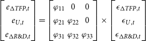 \begin{equation} \begin{bmatrix}e_{\Delta TFP,t} \\ e_{U,t}\\ e_{\Delta R\&D,t}\end{bmatrix}=\begin{bmatrix} \varphi _{11} & 0 & 0 \\ \varphi _{21} & \varphi _{22} & 0 \\ \varphi _{31} & \varphi _{32} & \varphi _{33} \end{bmatrix} \times \begin{bmatrix} \epsilon _{\Delta TFP,t} \\ \epsilon _{U,t}\\ \epsilon _{\Delta R\&D,t}\end{bmatrix} \end{equation}
To analyze the dynamic effects of structural shocks, we employ the following moving average representation:
 \begin{equation} Z_t=\Phi (L)\epsilon _t, \end{equation}
where $L$
is the lag and
$L$
is the lag and $\Phi (L)=\Phi _0+\Phi _1 L+\Phi _2 L^2 + \ldots = B(L)^{-1}S$
. The elements of the
$\Phi (L)=\Phi _0+\Phi _1 L+\Phi _2 L^2 + \ldots = B(L)^{-1}S$
. The elements of the $\Phi _h$
matrix describe the impact of the variable associated with the row on the one associated with the column after
$\Phi _h$
matrix describe the impact of the variable associated with the row on the one associated with the column after $h$
periods. These are the impulse response functions that we present in the next section.
$h$
periods. These are the impulse response functions that we present in the next section.
We use the Hannan-Quinn criterion for selecting the optimum lag length in our estimated VAR model, which is 5, while the Bayesian information criterion (BIC) suggests 2 and the Akaike information criterion (AIC) suggests 13. Results with 13 lags are identical, although the confidence bands are larger; therefore, we favor 5 over 13. Although we discuss results with 2 lags in section 6, here we justify our choice. We select 5 over 2 lags based on the link between R&D and TFP. Specifically, it takes time before the outcome of R&D materializes and manifests itself into higher TFP. How long it takes is largely an empirical question. Thus, we regress TFP growth on leads of R&D growth. The results presented in Table 1 indicate that the connection between R&D and TFP growth becomes significant only when the lead is more than three quarters. Moreover, the five-quarter lead shows the highest coefficient and R $^{2}$
. Looking at simple lagged correlations confirms the result. To avoid losing this piece of information about the connection between the two variables, we prefer a longer lag length.
$^{2}$
. Looking at simple lagged correlations confirms the result. To avoid losing this piece of information about the connection between the two variables, we prefer a longer lag length.
Table 1. Ordinary least squares (OLS) estimates
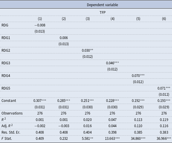
Note: The dependent variable is TFP growth. The independent variable is the 1st, 2nd, 3rd, 4th, and 5th lead of R&D growth, respectively. $^{*}$
p
$^{*}$
p $\lt$
0.1;
$\lt$
0.1; $^{**}$
p
$^{**}$
p $\lt$
0.05;
$\lt$
0.05; $^{***}$
p
$^{***}$
p $\lt$
0.01.
$\lt$
0.01.
5. Results
This section presents the results of the paper. We illustrate these results in the form of impulse responses of the three variables to exogenous changes in unemployment and TFP. First, we focus on impulse responses following an exogenous change in cyclical unemployment, which we interpret as the result of shocks that cause the business cycle. In this way, we test the hysteresis prediction generated by endogenous growth theory over the business cycle, which is the main endeavor of this paper. Second, we study the effect of an exogenous change in TFP to answer our supplementary question. This exercise allows us to identify which specific model produces results that are inconsistent with empirical evidence. Hence, we are able to rule out some of the mechanisms for the pro-cyclicality of R&D. Finally, we concentrate on the historical variance decomposition to gauge the quantitative importance of the mechanism we discuss. After doing that, we revisit the discussion on the productivity growth slowdown by pointing out how the business cycle interferes with the general understanding of the post-WWII aggregate productivity dynamics.
Exogenous change in cyclical unemployment
Figure 2 illustrates how R&D and utilization-adjusted TFP, in both levels and growth rates, respond to an exogenous rise in cyclical unemployment.
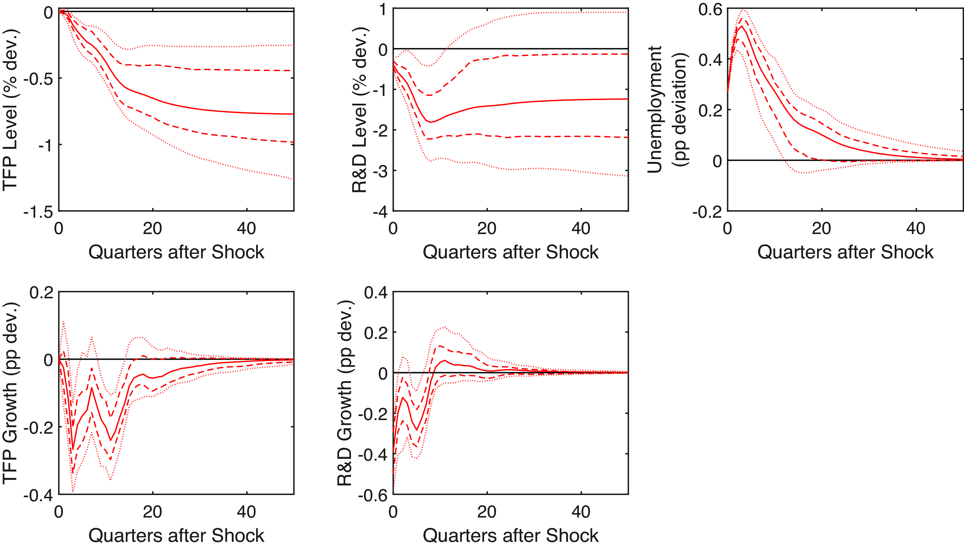
Figure 2. Unemployment shock. Note: Impulse responses in (annualized) growth rates and levels to a one standard deviation shock to the cyclical unemployment rate. The dashed and dotted lines are the 68% and 95% confidence bands, respectively. The black line is the pre-shock trend.
Our findings align with the main theoretical prediction. R&D is pro-cyclical and jumps immediately as the shock hits the economy. Productivity moves pro-cyclically as well but does so more slowly. The figure shows two drops in R&D growth, followed by two drops in TFP growth after about four quarters. Indeed, TFP’s response is consistent with the idea that R&D causes it to move with some lags.
Our analysis finds evidence of hysteresis and highlights its quantitative relevance. Specifically, when cyclical unemployment peaks at 1 percentage point above its average (equivalent to a two standard deviation shock), aggregate productivity experiences a permanent decline of approximately 1.3%. (Note: Figure 2 presents impulse responses to a one standard deviation shock.) The effect is large even though the deviation of TFP growth from its pre-shock value is not particularly large (it peaks at an annualized rate of 0.5 percentage points).
The large level effect is due to the persistence of the shock and of the R&D and TFP responses. Unemployment returns to its pre-shock level (based on the 68% bands) after more than 15 quarters. Likewise, TFP growth exhibits comparable persistence, causing its deviations from the trend to accumulate over time and generate large level effects.
Exogenous change in total factor productivity
We now consider an exogenous increase in TFP, shown in Figure 3. First, it is interesting to notice that the behavior of unemployment is the same as the one observed in Galí (Reference Galí1999), then replicated in the literature under different assumptions (Basu et al. Reference Basu, Fernald and Kimball2006; Li, Reference Li2022), following a technology shock, despite a different identification strategy and the use of different measures.
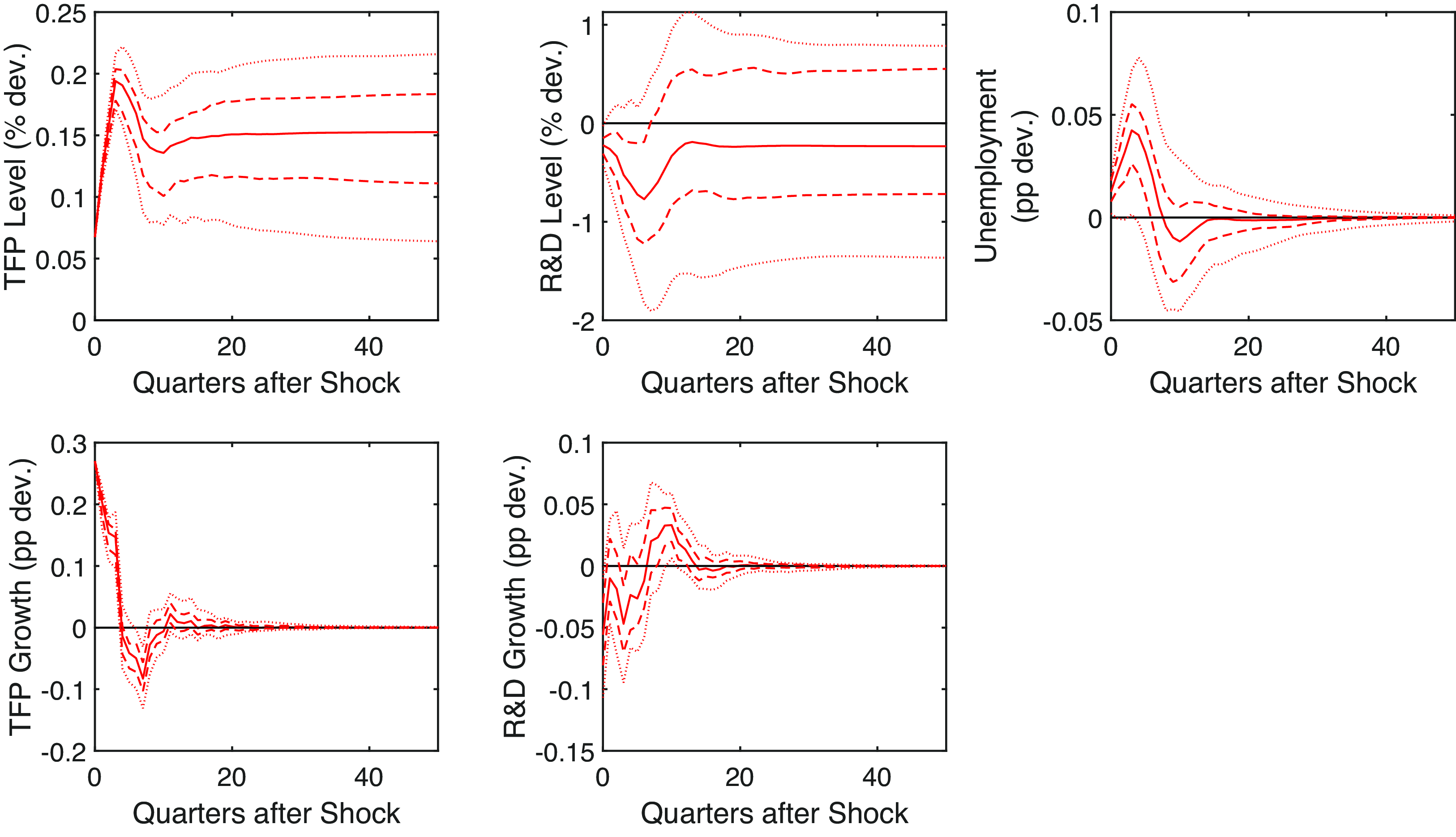
Figure 3. TFP shock. Note: Impulse responses in (annualized) growth rates and levels to a one standard deviation shock to utilization-adjusted TFP growth. The dashed and dotted lines are the 68% and 95% confidence bands, respectively. The black line is the pre-shock trend.
Of greater relevance to this study is the observed behavior of R&D. R&D initially decreases following a positive exogenous increase in productivity, although the effect is small. This result is in line with Schumpeter’s seminal idea that opened the field of R&D over the business cycle. In that view, R&D should move counter-cyclically as moving resources away from it and toward production in periods of higher profitability is convenient.
A few quarters after the initial decline in R&D, TFP growth reverses course and turns negative. An interpretation of these results is that this pro-cyclical opportunity cost of R&D produces a counter-cyclical behavior of R&D following a productivity shock. Then, the feedback mechanism from R&D to productivity produces a series of oscillations that die off after a couple of direction changes. The effect on TFP is permanent, while the long-run effect on R&D is not statistically different from 0. However, its confidence bands include an increase equal to the one on TFP.
This finding is particularly useful as it helps rule out certain theories explaining R&D’s pro-cyclicality. Theories where the pro-cyclicality emerges from the pro-cyclicality of profits would predict an increase in R&D following an increase in TFP. The theories whose predictions align with our results are those where the pro-cyclicality stems from financial frictions or from New Keynesian features.
How important is the business cycle for R&D and TFP?
Analyzing the forecast error variance decomposition helps identify the key factors driving fluctuations in the three time series. In this subsection, we show the contribution of exogenous changes in unemployment to the overall variation in R&D growth and TFP growth. Based on that, we examine how the path of those variables over the sample period would have differed in the absence of shocks driving changes in unemployment.
As Figure 4 shows, the variance of TFP growth is mostly explained by innovations in the TFP time series itself. This means that the majority of the variation in TFP at any frequency is the result of dynamics unrelated to the main business cycle shock, in accordance with the results obtained in Angeletos et al. (Reference Angeletos, Collard and Dellas2020). The same is true for R&D: most of the deviation in R&D is explained by its own exogenous evolution. However, we add to this existing evidence that although exogenous changes in unemployment are not the primary drivers of fluctuations in TFP growth, persistent shocks and R&D responses push TFP growth away from its long-run value persistently. Over time, these persistent deviations accumulate, resulting in significant long-term productivity losses.
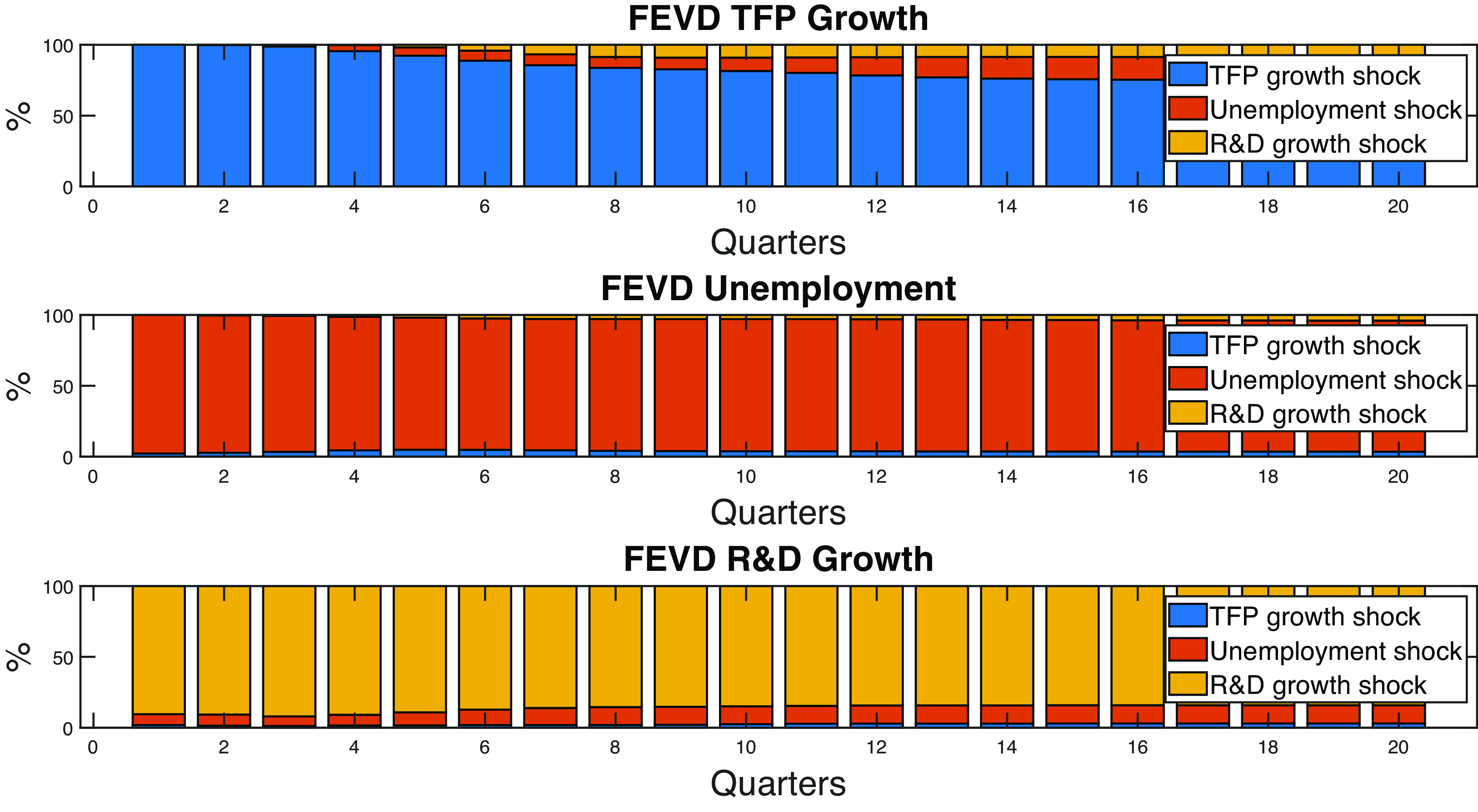
Figure 4. Forecast error variance decomposition.
Before illustrating this final point further, we must point out some caveats. Readers should interpret our findings as evidence that this mechanism generates substantial effects on average. After all, our main goal is to motivate further research on this topic as opposed to pointing out precise estimates of the effect of each shock on TFP in recent US history. Readers should note that our analysis assumes the VAR parameters remain constant over time. Additionally, we assume that positive and negative shocks exert symmetric effects, differing only in direction. We also assume that a change in their magnitude would be manifested in a proportional change in the response of all variables. Finally, we do not distinguish between different shocks as we assume that each shock that pushes unemployment away from its natural rate by a specific amount has the same effect on the other variables. We consider relaxing any of these assumptions an interesting future research pursuit motivated by our quantitatively large results.
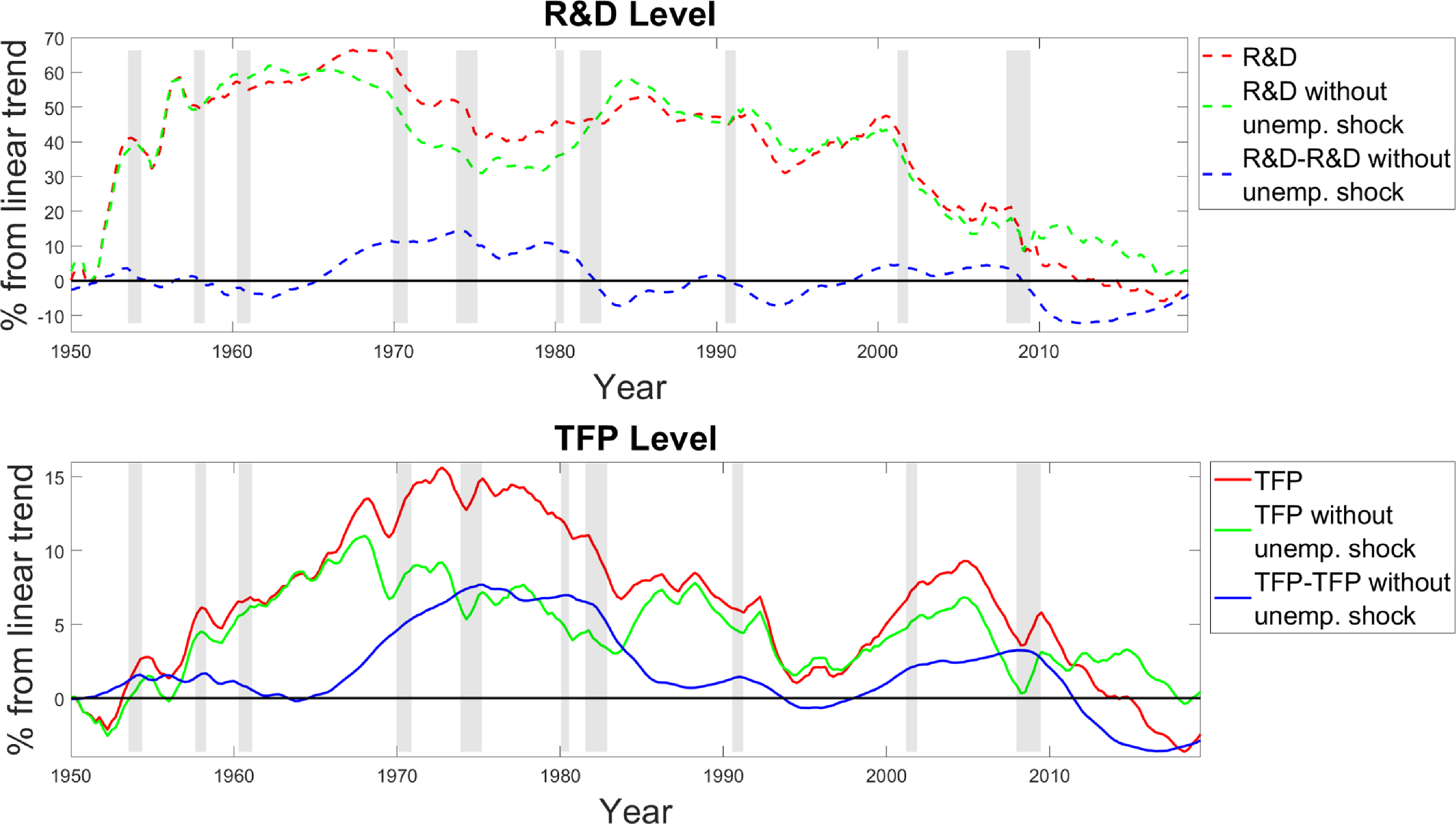
Figure 5. Log deviation from linear trend of TFP and R&D.
To estimate the long-run effect of business cycle shocks on productivity and R&D, we perform a historical decomposition using the SVAR model, depicted in Figure 5. We generate a counterfactual scenario by shutting down the unemployment shocks identified in the model. The resulting artificial data series represents how TFP and R&D would have evolved in the absence of these shocks. Comparing the actual series to this counterfactual allows us to quantify the cumulative impact of cyclical unemployment shocks on long-term innovation and productivity levels. Furthermore, Figure 6 depicts the blue lines of Figure 5, to better illustrate the connection between R&D and TFP. A noticeable feature of this graph, better visible in Figure 6, is the large drop in R&D during most recessions, followed by a gradual decline in TFP thereafter.
The first thing to notice from Figure 5 is that in the second panel, the green and the red lines move in tandem most of the time; that is, the blue curve is usually nearly flat. This result implies that most of the movement in TFP level is driven by causes unrelated to the business cycle. However, the deviation between the two curves is occasionally large; that is, the blue curve slopes either upward or downward because of the hysteresis effect picked up by our estimation. In particular, we notice three periods where the effect that we study is particularly strong: the boom in the late 1960s and early 1970s, the Volcker disinflation period in the early 1980s, and the Great Recession. The Great Recession is of particular interest, given the existence of a lively debate on the reasons behind the productivity slowdown that occurred during that period. On one side of the debate (Fernald et al. Reference Fernald, Hall, Stock and Watson2017), the argument is that the productivity slowdown is largely unrelated to the Great Recession as it preceded it and it consisted of a drop in the productivity growth rate to a level that was similar to the one observed a decade before. On the other side (Anzoategui et al. Reference Anzoategui, Comin, Gertler and Martinez2019), the idea proposed is that the productivity growth slowdown was to a large extent an endogenous response to the Great Recession. Our results show that productivity growth started declining in 2004 for reasons unrelated to the business cycle. However, the loss in productivity relative to pre-shock trend from 2008 to 2015 is approximately 6%. For comparison, Anzoategui et al. (Reference Anzoategui, Comin, Gertler and Martinez2019, p. 96) state: “between the starting point of the recent productivity slowdown, 2005, and the end of our sample, 2015, total TFP declined by approximately 8 percentage points (relative to trend). The endogenous component accounts for around 6 percentage points of decline.” The quantitative similarity between these two results is remarkable as our estimate comes from a VAR, while their estimate comes from a calibrated DSGE model.
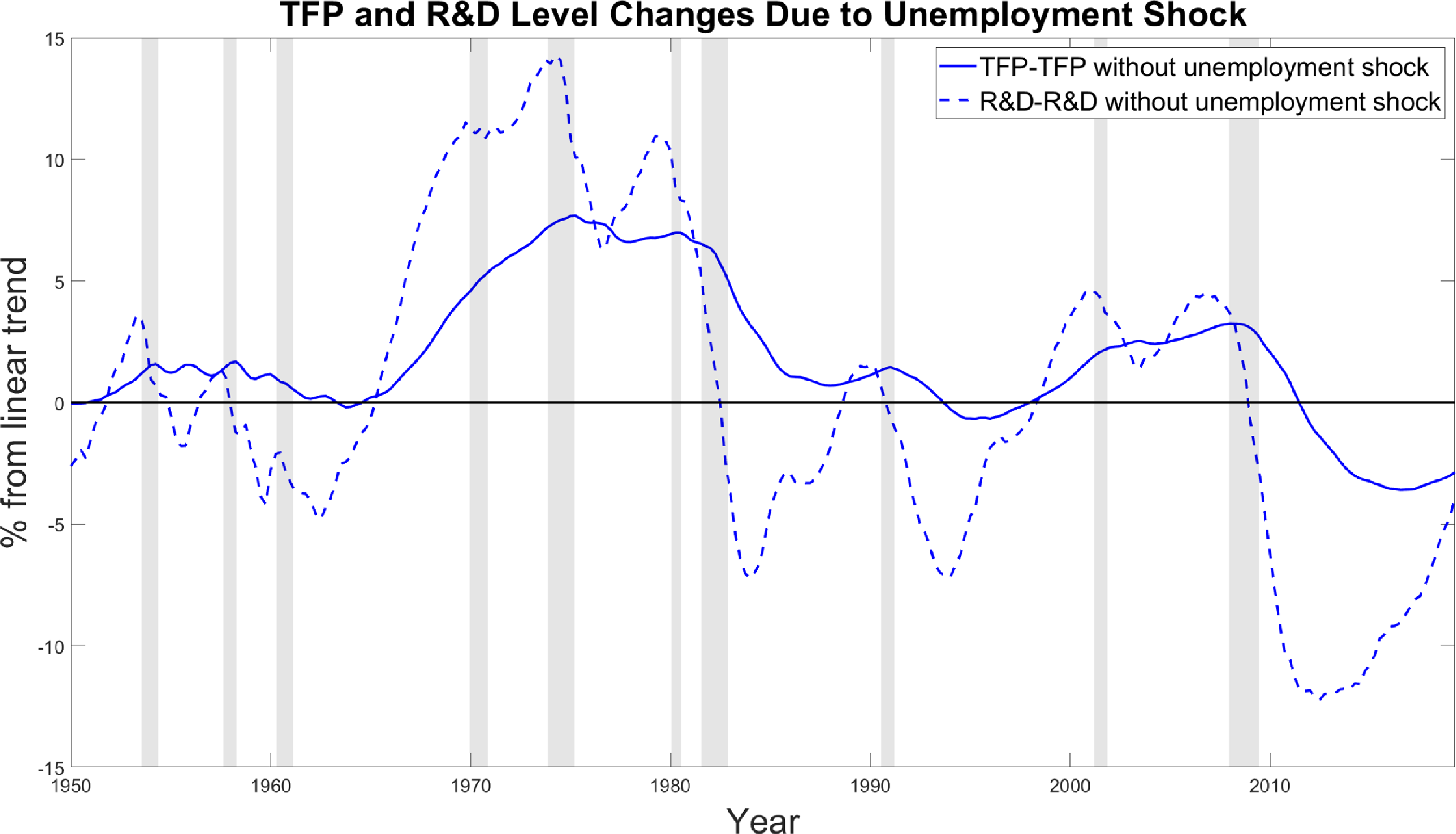
Figure 6. Log deviation from linear trend of TFP and R&D caused by exogenous changes in cyclical unemployment.
Revisiting the productivity growth slowdown
In public discourse, the productivity growth slowdown has attracted much attention. Although discussions on this topic tend to be vague on how this slowdown looks like, in the data, Fernald (Reference Fernald2015a, Reference Fernaldb) elucidates on the medium-term dynamics of aggregate productivity growth in the post-WWII period. Specifically, he interprets these dynamics as alternations of higher productivity growth periods with lower productivity growth periods. Using the structural breaks that he proposes, average aggregate productivity growth is high between 1948Q1 and 1973Q1 and between 1996Q1 and 2004Q3. It is instead low between 1973Q2 and 1995Q4 and between 2004Q4 and the latest observation available. Through our analysis, we can construct a synthetic time series of “cycle-free” aggregate productivity growth by dismissing changes in aggregate productivity growth that, according to our SVAR, result from deviations in cyclical unemployment to further inform this debate.
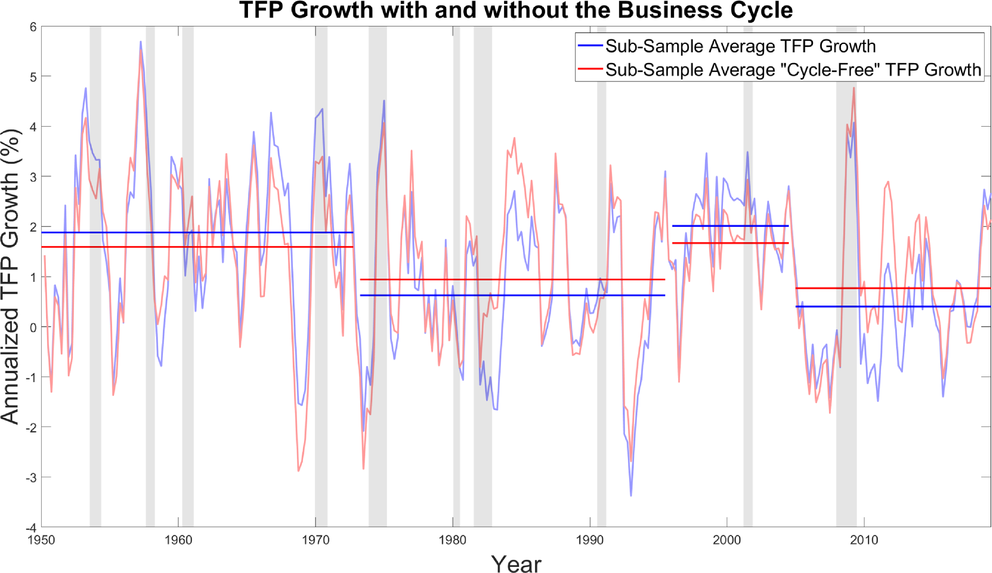
Figure 7. Sub-sample average of productivity growth in the data and subtracting away deviations caused by the unemployment shock in the SVAR. The breaks follow Fernald (Reference Fernald2015a, Reference Fernaldb).
Our results, depicted in Figure 7, show that the difference between growth rates in high versus low growth periods is noticeably shrunk once we remove the effect of the business cycle. Our procedure attributes approximately half of the difference in growth rates between high and low growth periods, equivalent to approximately 0.6 percentage points, driven by shocks that cause fluctuations in cyclical unemployment. Notice, however, that the light blue and light red line exhibits a very strong correlation. This figure illustrates clearly one of the results of this paper. In the absence of the business cycle, the pattern of TFP growth would look similar to the one observed in the data. That is, most of the variation in TFP growth is not explained by the business cycle shock. However, the systematic and persistent deviations caused by the business cycle shock ensure that TFP growth on average is different from what it would be in the absence of the business cycle.
6. Robustness
Our results remain robust across various specification changes. In this section, we illustrate all these changes.
Lag length choice
We run the VAR using different lag lengths, as various criteria suggest different optimal values. According to AIC, the optimal lag length is 13. The results are qualitatively and quantitatively similar, with the exception that the confidence bands are larger. However, the statistical significance of our results is not affected. According to BIC, the optimal lag length is 2. The results, shown in Figures 8 and 9 are slightly different in that the impulse response functions are smoother. However, the quantitative permanent effect of the business cycle shock on productivity is the same. Our conclusions, therefore, remain the same: the hysteresis effect is present and large enough to justify further scrutiny from macroeconomists.
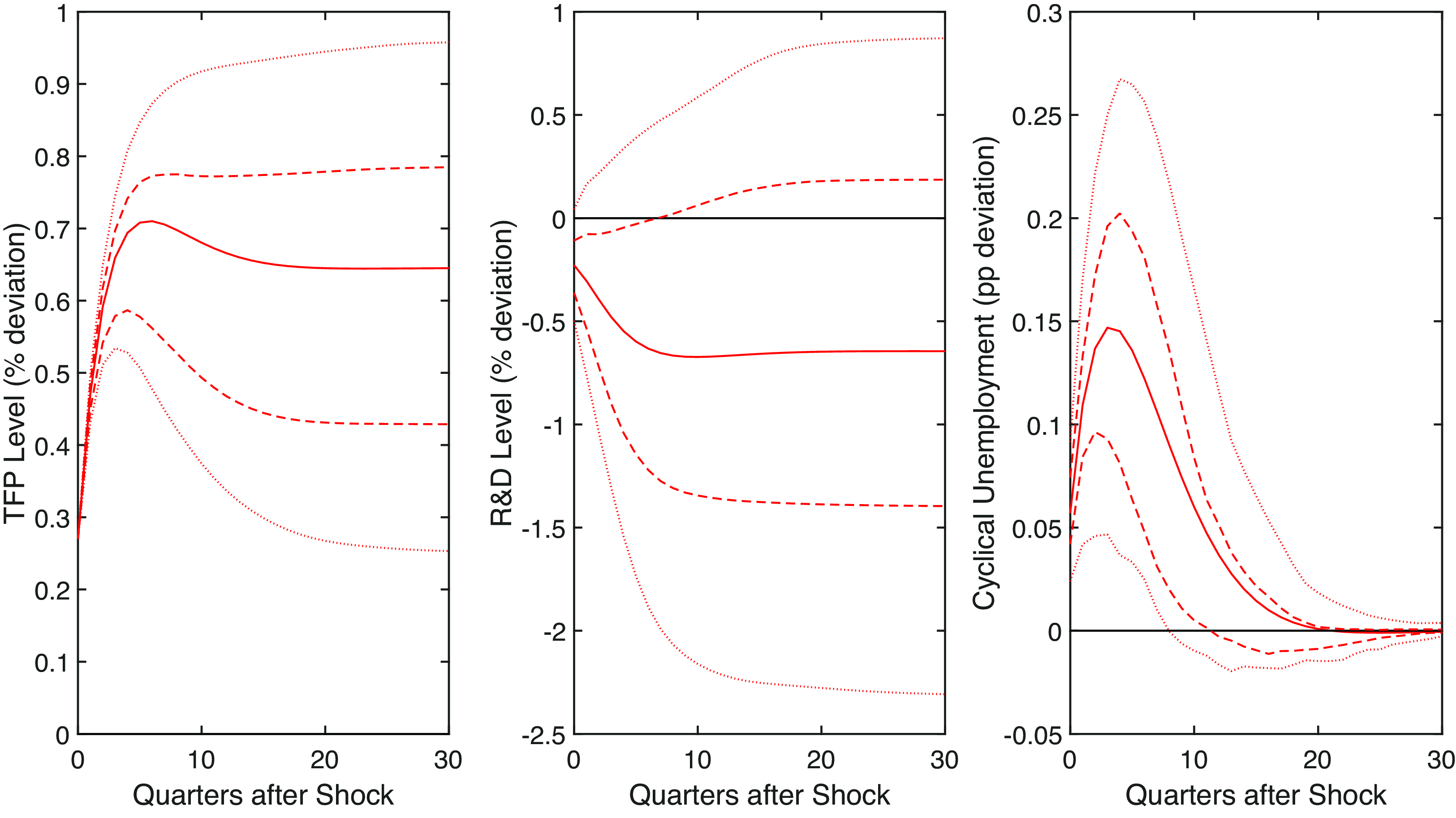
Figure 8. TFP shock. Note: Impulse responses in levels to a one standard deviation shock to utilization-adjusted TFP growth with lag of 2. The dashed and dotted lines are the 68% and 95% confidence bands, respectively. The black line is the pre-shock trend.
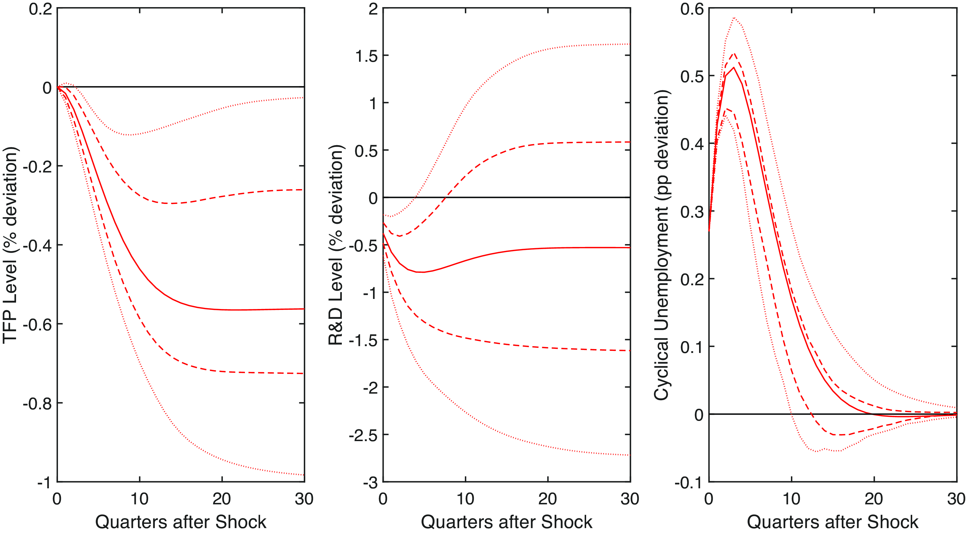
Figure 9. Unemployment shock. Note: Impulse responses in levels to a one standard deviation shock to the cyclical unemployment rate with lag of 2. The dashed and dotted lines are the 68% and 95% confidence bands, respectively. The black line is the pre-shock trend.
Alternative short-run restrictions
We now change the order of the variables in the VAR specification. This procedure changes the short-run restrictions. The first exercise we produce is to order unemployment first, followed by TFP growth and R&D growth, respectively. However, we introduce an additional restriction, namely, that TFP growth does not react on impact to a change in unemployment, which is the same restriction as in our preferred specification. Ordering unemployment first ensures that a greater portion of unemployment variation is captured by the innovation in the R&D time series, arguably rendering the identification strategy more similar to Angeletos et al. (Reference Angeletos, Collard and Dellas2020). We note that the results are nearly identical.
Next, we change the order of the variables, assuming that an exogenous change in unemployment does not have a simultaneous impact on R&D. This adjustment to the VAR specification allows more unemployment variation to be attributed to innovations in the R&D time series, eliminating potential investment-driven effects on unemployment from the error term. The results differ in that an exogenous change in unemployment does not have an immediate impact on R&D, which follows by assumption, but everything else remains the same.
News shocks
A popular stream of literature is the one of technology news shocks. In this framework, rational agents who suddenly learn about the future state of productivity change their behavior, affecting macroeconomic variables. Hence, these changes could reflect changes in the information set of agents as opposed to changes in economic fundamentals. This literature has therefore developed the concept of TFP surprise shocks and TFP news shocks. A widely adopted approach, as demonstrated in Barsky and Sims (Reference Barsky and Sims2011), identifies news shocks by combining reduced-form shocks that maximize TFP fluctuations at a predetermined future period. The surprise news shock is instead what is left after accounting for that. We follow this route in proposing one of our robustness checks.
News shocks are relevant to our analysis in two key ways. First, Barsky and Sims (Reference Barsky and Sims2011, p.288) point out that “most of the theoretical work in the news area assumes that good news is ‘manna from heaven’—that is, agents receive word in advance that aggregate technology will exogenously change at some point in the future.” Instead, the theoretical framework behind our paper suggests that aggregate technology changes as a result of endogenous changes in R&D investment. That is, any shock that temporarily displaces R&D investment from its path, permanently affects the aggregate technology level. If real-world data generation follows endogenous growth theory, the news shock identification strategy may mistakenly classify a business cycle shock causing hysteresis as an exogenous event. That is, the change in productivity would be incorrectly labeled “manna from heaven” when instead it is the endogenous product of innovation efforts reacting to macroeconomic conditions. If, instead, the real world’s data generating process conforms to the news shock theoretical framework illustrated in the Barsky and Sims (Reference Barsky and Sims2011)’s quote above, while R&D responds positively to a positive news shock, our identification approach could mistakenly interpret an exogenous effect as an endogenous hysteresis effect.Footnote 5 Thus, incorporating news shocks into the VAR serves as a valuable robustness check.
Second, our supplementary question, regarding which channel of pro-cyclicality is more plausible, relies on studying impulse responses to a TFP shock. However, the news shock literature divides the TFP shock in news and surprise shocks. Our preferred strategy is to rely on the utilization-adjusted TFP measure as in Basu et al. (Reference Basu, Fernald and Kimball2006) and add short-run restrictions, but this TFP shock could be masking a news shock. Consequently, we want to test whether the TFP shock effect disappears once we account for the news shock.
Rather than identifying news shocks independently, we incorporate the time series of news shocks from Kurmann and Sims (Reference Kurmann and Sims2021) as a variable in our VAR model with short-run restrictions. We order the news shock variable first, to ensure that it picks up as much of the variation as possible, while ordering the remaining three variables as in our main specification. This adjustment results in some data loss, as Kurmann and Sims (Reference Kurmann and Sims2021) estimate a VAR with four lags from 1960Q1 to 2007Q3, meaning the news shock time series spans 1961Q1–2007Q3. The results presented in Figures 10, 11 and 12 closely resemble earlier findings, with impulse responses to a news shock mirroring those in Kurmann and Sims (Reference Kurmann and Sims2021). Hence, we conclude that all our results are robust to the introduction of a TFP news shock.
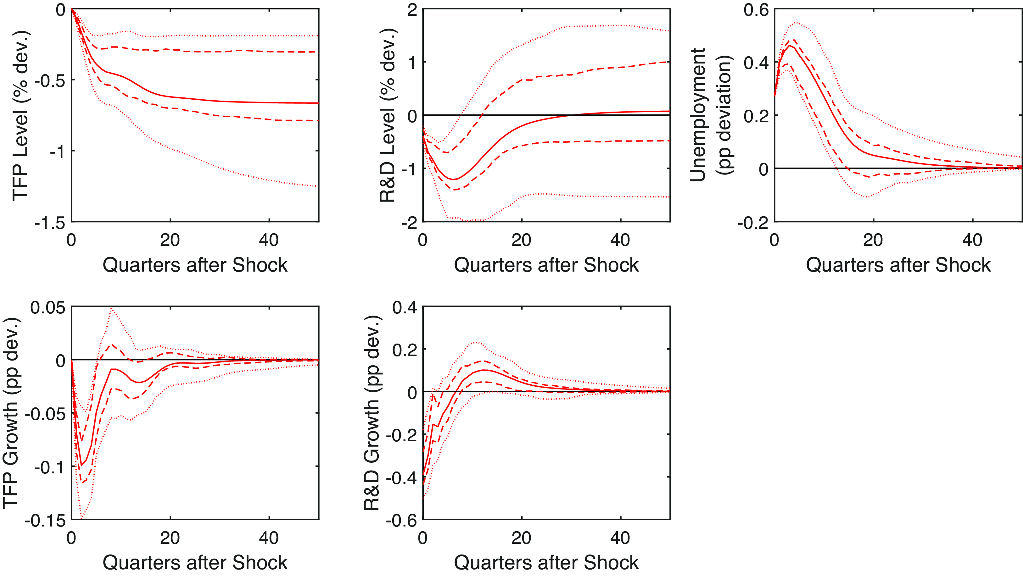
Figure 10. Unemployment shock in the model with news. Note: Impulse responses in levels and growth to a one standard deviation shock to the cyclical unemployment rate in the model that includes the news shock. The dashed and dotted lines are the 68% and 95% confidence bands, respectively. The black line is the pre-shock trend.
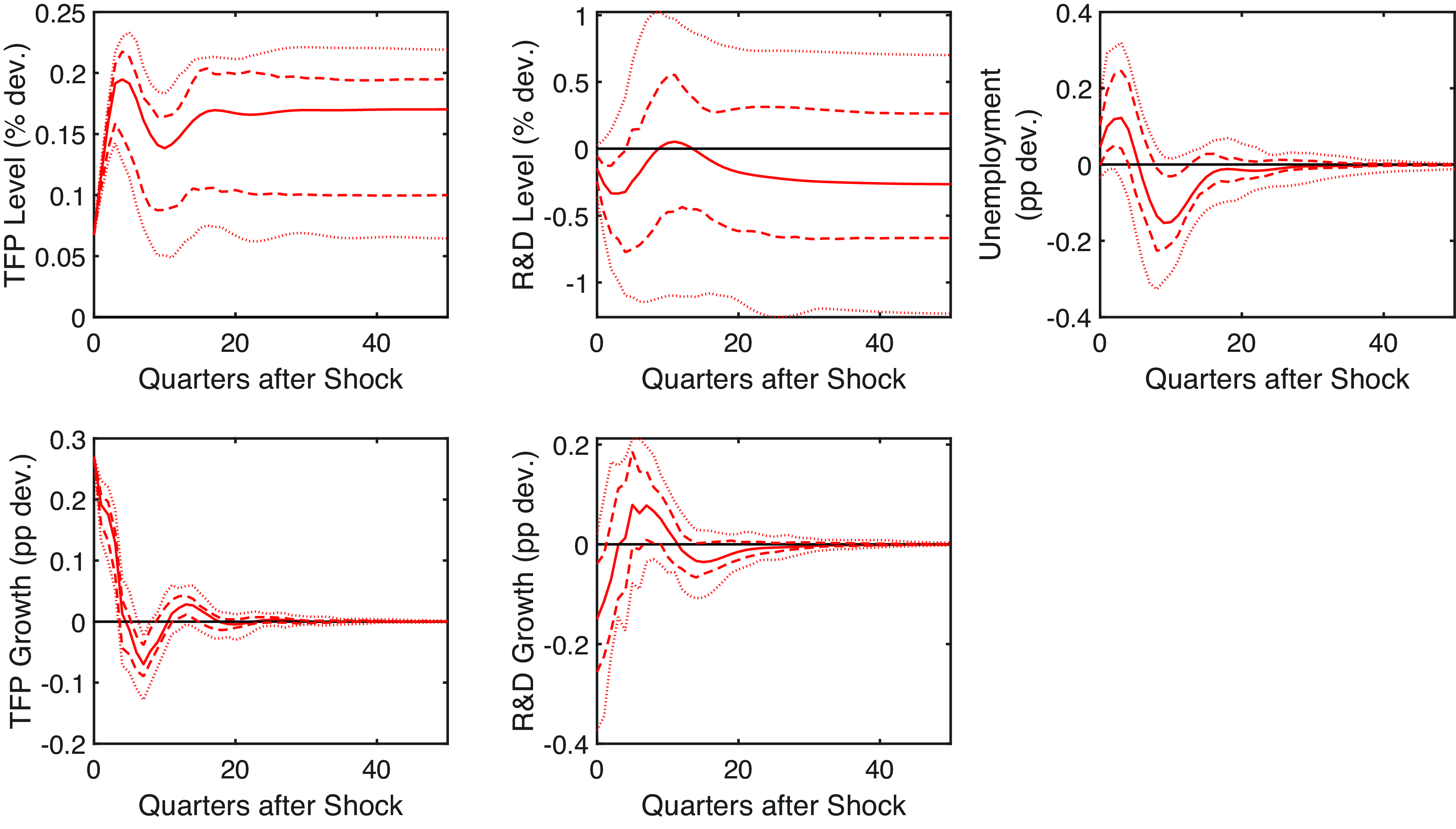
Figure 11. TFP shock in the model with news. Note: Impulse responses in levels to a one standard deviation shock to utilization-adjusted TFP in the model that includes the news shock. The dashed and dotted lines are the 68% and 95% confidence bands, respectively. The black line is the pre-shock trend.
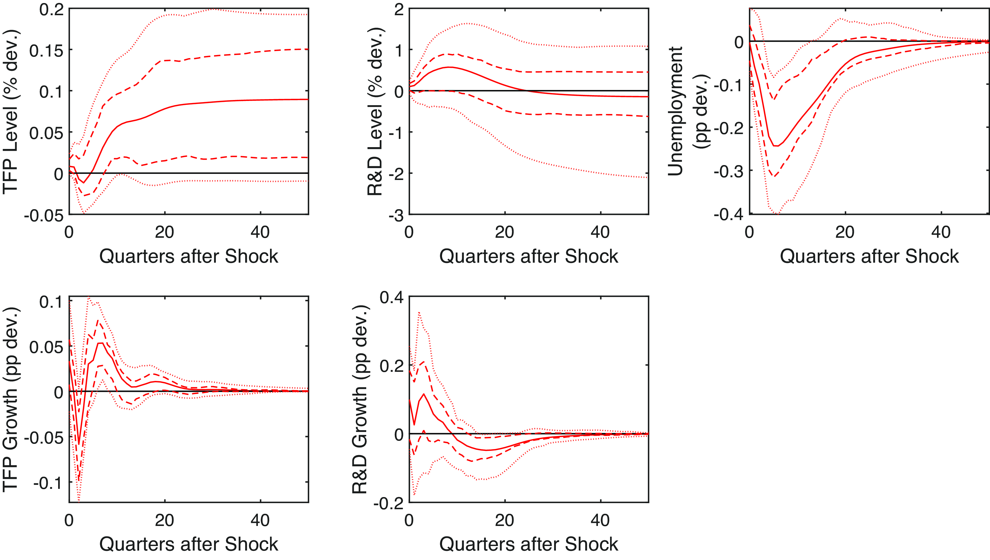
Figure 12. News shock. Note: Impulse responses in levels to a one standard deviation news shock. The dashed and dotted lines are the 68% and 95% confidence bands, respectively. The black line is the pre-shock trend.
VAR size and alternative identification
In this subsection, we increase the size of the VAR. Because the number of restrictions needed to identify shocks scales with the number of variables, we change the identification strategy. In this way, we avoid imposing controversial short-run restrictions. Instead, we include as a variable the main business cycle shock identified in Angeletos et al. (Reference Angeletos, Collard and Dellas2020), that is, the combination of reduced form shocks that maximizes changes in unemployment in the frequency domain between 6 and 32 quarters. Following Angeletos et al. (Reference Angeletos, Collard and Dellas2020), we compute the impulse responses to the orthogonalized shocks from a Bayesian VAR with Minnesota prior adjusting the prior mean to 0 because we enter the non-stationary variables in growth rate. The other variables that we include are real investment growth, consumption growth, GDP growth, inflation, hours worked growth, and the federal funds rate. The sample period spans 1955Q1–2017Q4.
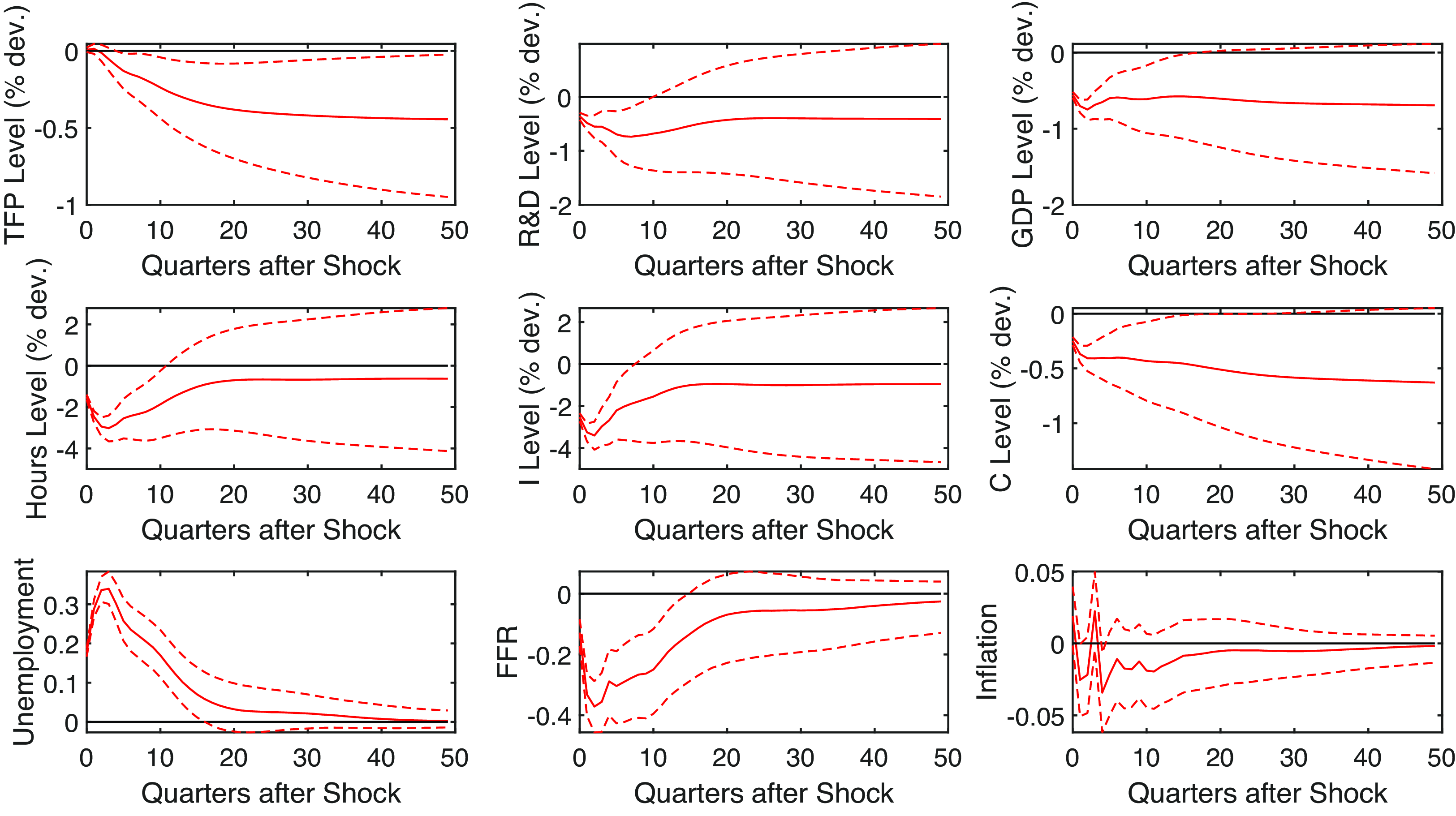
Figure 13. Main business cycle shock in a large VAR. Note: Impulse responses in levels to a one standard deviation main business cycle shock as identified in Angeletos et al. (Reference Angeletos, Collard and Dellas2020). For unemployment, inflation, and federal funds rate, the dashed 68% credible intervals. The other variables are the cumulated impulse response functions, and the dashed lines are the cumulated 16th and 84th percentile of the posterior distribution of impulse response functions.
Figure 13 shows the impulse response of all variables to the main business cycle shock. We notice that the behavior of R&D and TFP is the same as in our main estimation. The only exception is that TFP reacts counter-cyclically on impact, before declining shortly after, but this initial effect is small. For a 1 percentage point increase in unemployment, the long-run effect on the TFP level is a 1.3% reduction relative to pre-shock trend, the same as in our preferred specification.
Additional robustness checks
We now present a few minor robustness tests. First, when considering R&D, we would have to bear in mind a large policy change in 1982, with the introduction of an R&D tax credit. To account for this, we estimate the model twice: first using data up to 1981Q4, then with data from 1982Q1 onward. The results are almost identical.
Second, we modify the TFP time series. First, we look at utilization-adjusted TFP without taking the moving average. Then, we consider TFP, without the adjustment for factor utilization. In both cases, the long-run effect is quantitatively very similar. The difference is in the short-run, as an exogenous increase in unemployment determines an increase in TFP a quarter later. This change is most likely not reflective of changes in technological knowledge.
Third, we check for robustness under different transformations of TFP. In our main specification, TFP growth is smoothed using a four-period moving average. Using an eight-period moving average yields identical results. When we do not smooth the variable, TFP is counter-cyclical within the first couple of quarters, but then it follows the same path as in our preferred test, showing a long-run result that is slightly smaller. In that case, a 1 percentage point increase in unemployment causes a 1% hysteresis effect on the TFP level.
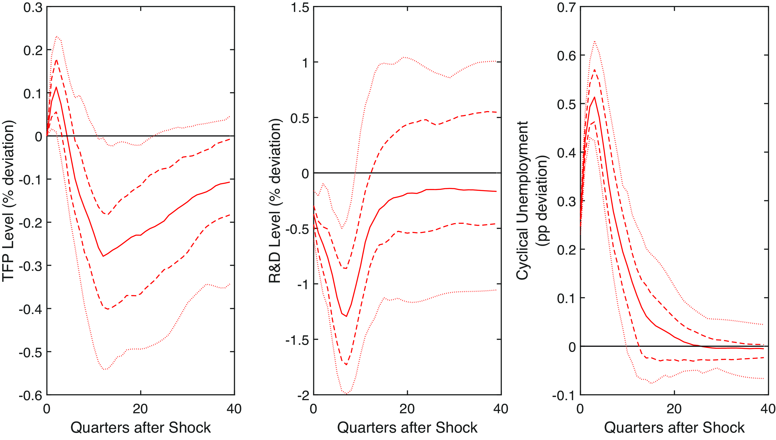
Figure 14. Unemployment shock (levels). Note: Impulse responses a one standard deviation shock to the cyclical unemployment rate. The dashed and dotted lines are the 68% and 95% confidence bands, respectively. The black line is the pre-shock trend. The model is estimated with TFP and R&D entering in levels.
Next, instead of entering TFP and R&D in log differences in the VAR, we enter them in log levels. This change rules out by assumption the presence of a permanent effect. The results, in Figures 14 and 15, show that indeed TFP reverts to the mean after an exogenous change in unemployment, while the results at other time horizons are robust. The only qualitative difference is the behavior of R&D following a positive exogenous change in TFP: R&D still decreases, but only a couple of quarters after the shock, and only the 68% bands show statistical significance. On the quantitative side, the response of TFP to a change in cyclical unemployment is smaller than in our preferred estimation, keeping in mind that the model specification is forcing it to revert. Specifically, TFP declines by 0.6% for an increase in unemployment that peaks at 1 percentage point above its mean. This effect is one-third of the one estimated with the model in growth rates. Nevertheless, the effect is still quantitatively relevant, thus supporting the main conclusion of this paper.
Finally, we replace unemployment with hours worked as the key variable. We detrend hours in two different ways, first by using the HP-filter, then by considering hours per capita. The results do not change.
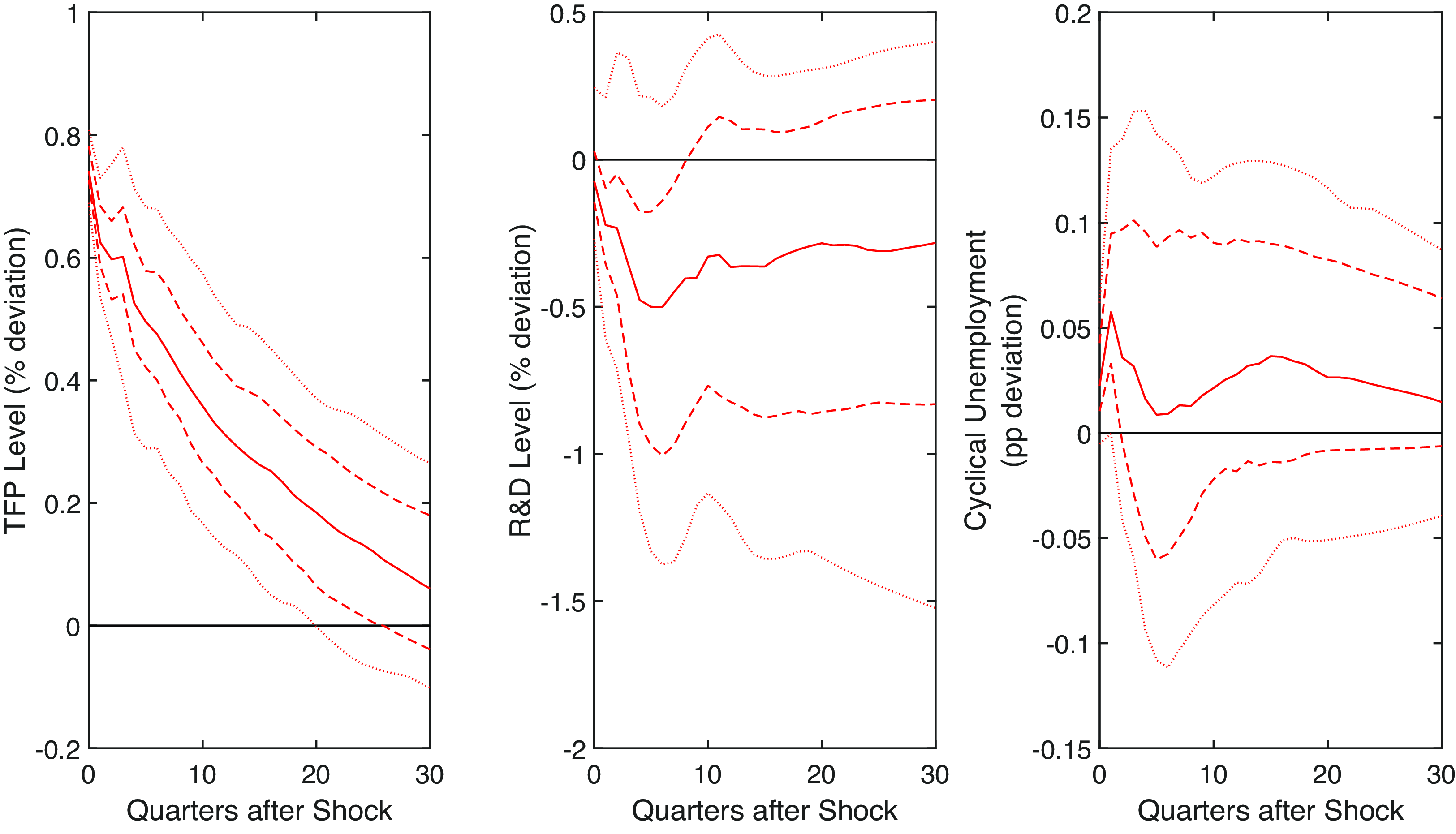
Figure 15. TFP shock (levels). Note: Impulse responses in (annualized) growth rates and levels to a one standard deviation shock to utilization-adjusted TFP. The dashed and dotted lines are the 68% and 95% confidence bands, respectively. The black line is the pre-shock trend. The model is estimated with TFP and R&D entering in levels.
7. Discussion and conclusion
This paper examines the predictions of endogenous growth theory in the context of business cycle disturbances. These models predict hysteresis, as shocks that temporarily move economic activity away from its trend affect the trend itself because R&D exhibits a pro-cyclical behavior. The idea behind this mechanism is that, since technological knowledge is cumulative, a temporary reduction in the flow of knowledge creation permanently reduces its stock.
By focusing on post-WWII US data, we employ a recursive VAR with three variables: cyclical unemployment, aggregate R&D spending, and utilization-adjusted TFP. We identify exogenous changes in cyclical unemployment and interpret them as an all-encompassing proxy for shocks that drive economic fluctuations at business cycle frequency. Our primary objectives are to evaluate whether R&D and TFP behave as predicted by theory and to quantify the significance of these responses.
First, we confirm that R&D reacts pro-cyclically to an increase in unemployment, and TFP follows with a lag. This result supports theoretical predictions and previous empirical evidence on R&D’s pro-cyclicality (Barlevy, Reference Barlevy2007; Ouyang, Reference Ouyang2011), underscoring the relevance of these models. We find that this effect is large: A temporary increase in cyclical unemployment that peaks at 1 percentage point above its sample average produces a permanent TFP loss of about 1.3%. This effect is substantial because the shock identified by our methodology is highly persistent. Consequently, even minor deviations in TFP growth accumulate over time, significantly impacting long-term productivity levels.
Through a historical variance decomposition, we further determine that this effect is particularly noticeable during the boom of the 1960s, during the Volcker disinflation years, and during the Great Recession. Our results therefore introduce further information on the debate relative to the connection between the productivity growth slowdown and the Great Recession. While a camp, see, for example, Fernald et al. (Reference Fernald, Hall, Stock and Watson2017), attributes the slowdown to causes that precede and are independent of the Great Recession, another camp, see, for example, Anzoategui et al. (Reference Anzoategui, Comin, Gertler and Martinez2019), attributes the same slowdown to the Great Recession and specifically to the deteriorated financial conditions. Our analysis supports both perspectives; however, our quantitative results closely align with those of Anzoategui et al. (Reference Anzoategui, Comin, Gertler and Martinez2019), despite employing a different methodology.
Despite the magnitude of our findings, most TFP variation remains independent of business cycle fluctuations. This result aligns with existing literature, for example, Angeletos et al. (Reference Angeletos, Collard and Dellas2020). The coexistence of substantial hysteresis effects and a TFP variation that is largely unexplained by business cycle shocks can be understood as follows: while exogenous changes in TFP are independently distributed and tend to balance out over time, persistent business cycle shocks cause a sustained deviation of TFP growth from its trend. Since this deviation moves in a single direction following a business cycle shock, it can influence average TFP growth over several years without accounting for much of its overall variation.
We acknowledge certain limitations in our analysis, despite conducting extensive robustness checks. Specifically, the SVAR assumes constant parameters that describe the relationship between the three variables and symmetric impulse responses. Furthermore, we do not distinguish between various sources of shocks. What we can say with confidence is that, when a shock displaces economic activity from its trend, the historical record suggests that hysteresis is present and quantitatively relevant on average. This is especially true for very persistent shocks. Based on these findings, we believe that exploring the issue further by relaxing these assumptions is a promising avenue for future research.
A supplementary result we uncover is that R&D initially declines following an exogenous TFP increase. This result is relevant as it helps in determining what drives R&D’s pro-cyclical behavior. Models where R&D is pro-cyclical due to profit’s pro-cyclicality are hard to reconcile with our result. In these models, a positive TFP shock increases expected short-term future profits, thus leading firms to conduct more R&D.
Instead, the result we obtain is consistent with predictions from models where financial frictions drive pro-cyclical R&D. These models include the Schumpeterian channel that gave rise to this stream of literature, namely, that following a boom resources are reallocated from R&D to production as the marginal value of production increases, increasing the opportunity cost of R&D. Thus, a TFP shock initially reduces R&D. However, credit constraints on R&D-intensive firms mean that negative shocks tightening financial conditions deplete available R&D funding. The behavior of R&D would vary depending on which shock hits the economy. Previous research emphasizes stronger pro-cyclicality in industries that are more reliant on external financing (van Ophem et al. Reference van Ophem, van Giersbergen, van Garderen and Bun2019). Our results reinforce that view. In addition, a body of literature that studies firm-level innovation responses to financial shocks or to shocks under financial constraints documents the same pro-cyclicality of firm-level R&D and TFP (Aghion et al. Reference Aghion, Askenazy, Berman, Cette and Eymard2012; Kabukcuoglu, Reference Kabukcuoglu2019; Duval et al. Reference Duval, Hong and Timmer2020) that are consistent with the impulse responses from business cycle shocks on aggregate data that our analysis produces.
Our finding is also consistent with results from an endogenous growth model with New Keynesian features (Aysun, Reference Aysun2020). The key insight stressed in this model is that R&D comoves positively with aggregate employment, as opposed to output. Therefore, positive productivity shocks, which in our analysis and in previous research (Galí, Reference Galí1999; Basu et al. Reference Basu, Fernald and Kimball2006; Li, Reference Li2022) reduce employment, also reduce R&D.
However, our study neither rules out the possibility that key drivers of R&D’s pro-cyclicality remain unidentified nor quantifies the impact of financial or labor market frictions on hysteresis. We leave this pursuit to future research.
In conclusion, the magnitude of our estimated effect underscores the need for further research on the link between business cycles and long-run growth, making it a priority for macroeconomists. In particular, the theoretical challenge is to explain why R&D is pro-cyclical following non-technology shocks yet declines in response to positive TFP shocks. Empirically, a valuable avenue for future research is identifying asymmetries in either the shocks driving R&D behavior or R&D’s responses, as suggested by Ouyang (Reference Ouyang2011). In this way, the economy’s volatility could be linked to its average growth rate.
Acknowledgments
We thank the editor, associate editor, three anonymous referees, and participants at our presentations in various conferences for helpful comments. All remaining errors are our own.


 Open access