


1. Introduction
One relatively simple way to evaluate the bootstrap current in stellarators is to use the long mean free path asymptotic formula of Shaing & Callen (Reference Shaing and Callen1983) which contains all the information about device geometry in a geometrical factor independent of plasma parameters. This way is especially suited for stellarator optimization (Beidler et al. Reference Beidler1990; Nakajima et al. Reference Nakajima, Okamoto, Todoroki, Nakamura and Wakatani1989) where multiple fast estimates of the bootstrap current are required. Despite the fact that it has been derived more than 40 years ago, the validity range of this formula still remains unclear. Although the same result is exactly (Helander, Geiger & Maassberg et al. Reference Helander, Geiger and Maassberg2011) or approximately (Boozer & Gardner Reference Boozer and Gardner1990) reproduced by different derivations, however, it is not reproduced in the $1/\nu$
regime by numerical modeling (Beidler et al. Reference Beidler2011). Namely, with decreasing normalized collisionality
$1/\nu$
regime by numerical modeling (Beidler et al. Reference Beidler2011). Namely, with decreasing normalized collisionality $\nu _\ast$
, the bootstrap coefficient does not come to a saturation at the asymptotic limit but rather shows a complicated behavior which is quite different at magnetic surfaces with different radii (Kernbichler et al. Reference Kernbichler, Kasilov, Kapper, Martitsch, Nemov and Heyn2016). In turn, in the presence of a radial electric field, numerical modeling shows a saturation to the Shaing–Callen limit with decreasing
$\nu _\ast$
, the bootstrap coefficient does not come to a saturation at the asymptotic limit but rather shows a complicated behavior which is quite different at magnetic surfaces with different radii (Kernbichler et al. Reference Kernbichler, Kasilov, Kapper, Martitsch, Nemov and Heyn2016). In turn, in the presence of a radial electric field, numerical modeling shows a saturation to the Shaing–Callen limit with decreasing $\nu _\ast$
. This feature of the bootstrap coefficient regularly observed in the drift kinetic equation solver, DKES (Hirshman et al. Reference Hirshman, Shaing, van Rij, Beasley and Crume1986; van Rij & Hirshman Reference van Rij and Hirshman1989) modeling, and later confirmed by various codes of different types (Beidler et al. Reference Beidler2011) has been pointed out to the authors of a paper by Henning Maassberg (Reference Maassberg2004) more than 20 years ago, and, together with the problem of bootstrap resonances (Boozer & Gardner Reference Boozer and Gardner1990), it was the main reason to start the development of the drift kinetic equation solver NEO-2 (Kernbichler et al. Reference Kernbichler, Kasilov, Leitold, Nemov and Allmaier2008; Kasilov et al. Reference Kasilov, Kernbichler, Martitsch, Maassberg and Heyn2014; Martitsch et al. Reference Martitsch2016; Kernbichler et al. Reference Kernbichler, Kasilov, Kapper, Martitsch, Nemov and Heyn2016; Kapper et al. Reference Kapper, Kasilov, Kernbichler, Martitsch, Heyn, Marushchenko and Turkin2016, Reference Kapper, Kasilov, Kernbichler and Aradi2018). Finally, we can present here the results of this long going effort.
$\nu _\ast$
. This feature of the bootstrap coefficient regularly observed in the drift kinetic equation solver, DKES (Hirshman et al. Reference Hirshman, Shaing, van Rij, Beasley and Crume1986; van Rij & Hirshman Reference van Rij and Hirshman1989) modeling, and later confirmed by various codes of different types (Beidler et al. Reference Beidler2011) has been pointed out to the authors of a paper by Henning Maassberg (Reference Maassberg2004) more than 20 years ago, and, together with the problem of bootstrap resonances (Boozer & Gardner Reference Boozer and Gardner1990), it was the main reason to start the development of the drift kinetic equation solver NEO-2 (Kernbichler et al. Reference Kernbichler, Kasilov, Leitold, Nemov and Allmaier2008; Kasilov et al. Reference Kasilov, Kernbichler, Martitsch, Maassberg and Heyn2014; Martitsch et al. Reference Martitsch2016; Kernbichler et al. Reference Kernbichler, Kasilov, Kapper, Martitsch, Nemov and Heyn2016; Kapper et al. Reference Kapper, Kasilov, Kernbichler, Martitsch, Heyn, Marushchenko and Turkin2016, Reference Kapper, Kasilov, Kernbichler and Aradi2018). Finally, we can present here the results of this long going effort.
Some of the reasons for the anomalous behavior of the bootstrap coefficient described above have been identified recently (Beidler Reference Beidler2020) by using the general solution of the ripple-averaged kinetic equation, GSRAKE (Beidler & D’haeseleer Reference Beidler and D’haeseleer1995), to determine the Ware-pinch coefficient, which is equivalent to the bootstrap coefficient due to Onsager symmetry. Although instructive, these results are largely of a qualitative nature, and one of the main purposes of this paper is to treat this problem in a more analytical manner, with subsequent verification by numerical modeling using NEO-2 and a simplified propagator method in order to provide simple scalings and certain conditions useful for stellarator optimization. The challenges which such an endeavor must face will also be illustrated by considering the extreme example of a so-called anti-sigma configuration – the antithesis of the model field considered in Mynick, Chu & Boozer (Reference Mynick, Chu and Boozer1982) – for which the bootstrap coefficient obviously diverges with decreasing collisionality over the entire $\nu _*$
range of DKES computations. A second purpose of this paper is to outline a simple numerical approach, utilizing the computations of the bootstrap coefficient in the
$\nu _*$
range of DKES computations. A second purpose of this paper is to outline a simple numerical approach, utilizing the computations of the bootstrap coefficient in the $1/\nu$
regime, to also allow computations in regimes where particle precession (in particular, due to the radial electric field) is important, thereby providing an effective tool for the optimization problem mentioned above.
$1/\nu$
regime, to also allow computations in regimes where particle precession (in particular, due to the radial electric field) is important, thereby providing an effective tool for the optimization problem mentioned above.
As shown below, for the ‘anomalous’ behavior of the bootstrap coefficient, the interaction between boundary layers separating co- and counter-passing particles from trapped particles and the layers separating different trapped particle classes from each other plays an important role. In collisionless asymptotic theories, these layers are assumed infinitely thin and non-overlapping. This cannot be fulfilled at irrational flux surfaces, where the number of trapped particle classes is infinite, while the width of the layers is finite at any collisionality. Another reason is the interaction of the trapped–passing boundary layer with itself, which happens in case of anti-sigma configurations where the magnetic field maximum at a given flux surface is reached on a line which splits the field line into non-equivalent segments exchanging transient particles via the boundary layer. In both cases, an important prerequisite for anomaly is a finite bounce-averaged cross-surface drift of trapped particles, which is absent in axisymmetric and nearly absent in sufficiently accurate quasi-symmetric configurations showing no anomalies of the bootstrap current (Landreman, Buller & Drevlak Reference Landreman, Buller and Drevlak2022).
We restrict our analysis here to the mono-energetic approach (Beidler et al. Reference Beidler2011) employing the Lorentz collision model, since this approach is sufficient for the account of main effects related to the magnetic field geometry. Effects of energy and momentum conservation pertinent to the full linearized collision model can be recovered then with good accuracy from the mono-energetic solutions of the kinetic equation using various momentum correction techniques (Taguchi Reference Taguchi1992; Sugama & Nishimura Reference Sugama and Nishimura2002, Reference Sugama and Nishimura2008; Maassberg, Beidler & Turkin Reference Maassberg, Beidler and Turkin2009). This mono-energetic approach is briefly outlined in § 2.1 where also the basic notation is introduced. In § 2.2 we re-derive the Shaing–Callen formula (Shaing & Callen Reference Shaing and Callen1983) within this approach in the $1/\nu$
transport regime in order to obtain an explicit solution for trapped particle distribution accounting for various trapped particle classes. The structure of this solution is quite demonstrative for the reasons behind the ‘anomalous’ behavior of the bootstrap current mentioned above. In that section, we also extend the alternative derivation of Helander et al. (Reference Helander, Geiger and Maassberg2011) within the adjoint approach to the next order in collisionality. Although the obtained correction has no effect on the resulting Ware-pinch (bootstrap) coefficient, it is useful for understanding a certain paradox contained in this solution. Collisionless asymptotic solutions are compared with numerical solutions for finite plasma collisionality in § 2.3 where the cases with convergence of these solutions to the Shaing–Callen limit at low collisionality are demonstrated. In § 3 we examine the effect of collisional boundary layers on the distribution function in the adjoint (Ware pinch) problem where they lead to the off-set of this function from the value of collisionless asymptotic of Helander et al. (Reference Helander, Geiger and Maassberg2011) and respective off-set of the Ware-pinch coefficient. In particular, in § 3.2 we introduce a simplified approach (propagator method) to describe this off-set in the leading order over collisionality with help of a set of Wiener–Hopf-type integral equations. This set is infinite in the case of irrational field lines, and becomes finite for closed field lines. In § 3.3, with the help of this set, we derive the conditions on the equilibrium magnetic field required to avoid the leading-order off-set. We obtain a simple expression for the distribution function off-set in the case these conditions are weakly violated in § 3.5, where we express these solutions via two discrete functions tabulated using the numerical solutions of two respective infinite integral equation sets resulting from the linearization of the original Wiener–Hopf-type set. In § 4 we examine the off-set of the distribution function and Ware-pinch coefficient at irrational flux surfaces both numerically, with the help of the NEO-2 code solutions at high-order rational magnetic field lines approximating the irrational surface (§ 4.1), and using the analytical estimates of the asymptotic behavior of the off-set with decreasing plasma collisionality (§ 4.2). A related issue of bootstrap resonances is briefly discussed in § 4.4. In § 5 we study the effect of banana orbit precession (in particular, due to a finite radial electric field) on the off-set of the Ware-pinch coefficient and formulate there a simple bounce-averaged approach for the account of this effect in computations of the Ware-pinch coefficient using the numerical solutions for the distribution function in the
$1/\nu$
transport regime in order to obtain an explicit solution for trapped particle distribution accounting for various trapped particle classes. The structure of this solution is quite demonstrative for the reasons behind the ‘anomalous’ behavior of the bootstrap current mentioned above. In that section, we also extend the alternative derivation of Helander et al. (Reference Helander, Geiger and Maassberg2011) within the adjoint approach to the next order in collisionality. Although the obtained correction has no effect on the resulting Ware-pinch (bootstrap) coefficient, it is useful for understanding a certain paradox contained in this solution. Collisionless asymptotic solutions are compared with numerical solutions for finite plasma collisionality in § 2.3 where the cases with convergence of these solutions to the Shaing–Callen limit at low collisionality are demonstrated. In § 3 we examine the effect of collisional boundary layers on the distribution function in the adjoint (Ware pinch) problem where they lead to the off-set of this function from the value of collisionless asymptotic of Helander et al. (Reference Helander, Geiger and Maassberg2011) and respective off-set of the Ware-pinch coefficient. In particular, in § 3.2 we introduce a simplified approach (propagator method) to describe this off-set in the leading order over collisionality with help of a set of Wiener–Hopf-type integral equations. This set is infinite in the case of irrational field lines, and becomes finite for closed field lines. In § 3.3, with the help of this set, we derive the conditions on the equilibrium magnetic field required to avoid the leading-order off-set. We obtain a simple expression for the distribution function off-set in the case these conditions are weakly violated in § 3.5, where we express these solutions via two discrete functions tabulated using the numerical solutions of two respective infinite integral equation sets resulting from the linearization of the original Wiener–Hopf-type set. In § 4 we examine the off-set of the distribution function and Ware-pinch coefficient at irrational flux surfaces both numerically, with the help of the NEO-2 code solutions at high-order rational magnetic field lines approximating the irrational surface (§ 4.1), and using the analytical estimates of the asymptotic behavior of the off-set with decreasing plasma collisionality (§ 4.2). A related issue of bootstrap resonances is briefly discussed in § 4.4. In § 5 we study the effect of banana orbit precession (in particular, due to a finite radial electric field) on the off-set of the Ware-pinch coefficient and formulate there a simple bounce-averaged approach for the account of this effect in computations of the Ware-pinch coefficient using the numerical solutions for the distribution function in the $1/\nu$
regime. A qualitative discussion of the off-set in the direct problem describing the bootstrap coefficient is presented in § 6 where we also examine the possibility of bootstrap effect at the magnetic axis. Finally, the results are summarized in § 7, where some implications for reactor optimization are also discussed.
$1/\nu$
regime. A qualitative discussion of the off-set in the direct problem describing the bootstrap coefficient is presented in § 6 where we also examine the possibility of bootstrap effect at the magnetic axis. Finally, the results are summarized in § 7, where some implications for reactor optimization are also discussed.
2. Asymptotic models and finite collisionality
In this section, we review asymptotical long mean free path models of the bootstrap and Ware-pinch effect in the set-up where all explicit and implicit assumptions used in derivations of those models are fulfilled. We use a standard method (Hinton & Hazeltine Reference Hinton and Hazeltine1976; Galeev & Sagdeev Reference Galeev and Sagdeev1979; Helander & Sigmar Reference Helander and Sigmar2002) to re-derive transport coefficients in both cases, with a main focus on the boundary conditions in the presence of multiple trapped particle classes. We verify these models by numerical computation and identify their applicability range and mechanisms responsible for discrepancies at finite collisionality.
2.1. Adjoint mono-energetic problems on a closed field line
For the present analysis of bootstrap current convergence with plasma collisionality, a mono-energetic approach is sufficient, where a Lorentz collision model and constant electrostatic potential within flux surfaces are assumed. The linear deviation of the distribution function $f$
from the local Maxwellian
$f$
from the local Maxwellian $f_M$
is presented as a superposition of thermodynamic forces
$f_M$
is presented as a superposition of thermodynamic forces $A_k$
as detailed in Kernbichler et al. (Reference Kernbichler, Kasilov, Kapper, Martitsch, Nemov and Heyn2016)
$A_k$
as detailed in Kernbichler et al. (Reference Kernbichler, Kasilov, Kapper, Martitsch, Nemov and Heyn2016)
 \begin{align} f-f_M = f_M \sum \limits _{k=1}^3 g_{(k)} A_k, \end{align}
where
 \begin{eqnarray} A_1 = \frac {1}{n_\alpha }\frac {\partial n_\alpha }{\partial r} -\frac {e_\alpha E_r}{T_\alpha }-\frac {3}{2T_\alpha }\frac {\partial T_\alpha }{\partial r}, \quad A_2 = \frac {1}{T_\alpha }\frac {\partial T_\alpha }{\partial r}, \quad A_3 = \frac {e_\alpha \langle E_\parallel B\rangle }{T_\alpha \langle B^2\rangle }, \end{eqnarray}
where, $e_\alpha$
,
$e_\alpha$
, $m_\alpha$
,
$m_\alpha$
, $n_\alpha$
and
$n_\alpha$
and $T_\alpha$
are the
$T_\alpha$
are the $\alpha$
species charge, mass, density and temperature, respectively,
$\alpha$
species charge, mass, density and temperature, respectively, $E_r$
,
$E_r$
, $E_\parallel$
are the radial (electrostatic) and parallel (inductive) electric field,
$E_\parallel$
are the radial (electrostatic) and parallel (inductive) electric field, $B$
is the magnetic field strength and
$B$
is the magnetic field strength and $\langle \ldots \rangle$
denotes a neoclassical flux surface average. This reduces the linearized drift kinetic equation in the
$\langle \ldots \rangle$
denotes a neoclassical flux surface average. This reduces the linearized drift kinetic equation in the $1/\nu$
regime to a set of independent equations
$1/\nu$
regime to a set of independent equations
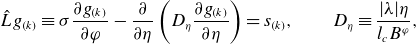 \begin{align} \hat L g_{(k)} \equiv \sigma \frac {\partial g_{(k)}}{\partial \varphi } -\frac {\partial }{\partial \eta }\left (D_\eta \frac {\partial g_{(k)}}{\partial \eta }\right )=s_{(k)}, \qquad D_\eta \equiv \frac {|\lambda |\eta }{l_c B^\varphi }, \end{align}
which differ only by source terms
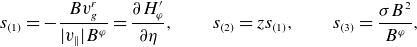 \begin{eqnarray} s_{(1)}\; &=&\; - \frac {B v_g^r}{|v_\parallel | B^\varphi } = \frac {\partial H_\varphi ^\prime }{\partial \eta }, \qquad s_{(2)} = z s_{(1)}, \qquad s_{(3)} = \frac {\sigma B^2}{B^\varphi }, \end{eqnarray}
where
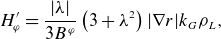 \begin{align} H_\varphi ^\prime = \frac {|\lambda |}{3 B^\varphi }\left (3 +\lambda ^2\right )|\nabla r|k_G \rho _L, \end{align}
will be integrated along the field line later to give bounce integrals $H_j$
in (2.26). Here, we use a field aligned coordinate system
$H_j$
in (2.26). Here, we use a field aligned coordinate system $(r,\vartheta _0,\varphi )$
, where
$(r,\vartheta _0,\varphi )$
, where $r$
is a flux surface label (effective radius) fixed by the condition
$r$
is a flux surface label (effective radius) fixed by the condition $\langle |\nabla r| \rangle = 1$
,
$\langle |\nabla r| \rangle = 1$
, $\vartheta _0=\vartheta - \iota \varphi$
is a field line label,
$\vartheta _0=\vartheta - \iota \varphi$
is a field line label, $\iota$
is the rotational transform and
$\iota$
is the rotational transform and $\vartheta$
and
$\vartheta$
and $\varphi$
are the poloidal and toroidal angles of periodic Boozer coordinates (Boozer Reference Boozer1981; d’Haeseleer et al. Reference d’Haeseleer, Hitchon, Callen and Shohet1991), respectively. Variables in the velocity space are parallel velocity sign
$\varphi$
are the poloidal and toroidal angles of periodic Boozer coordinates (Boozer Reference Boozer1981; d’Haeseleer et al. Reference d’Haeseleer, Hitchon, Callen and Shohet1991), respectively. Variables in the velocity space are parallel velocity sign $\sigma =v_\parallel /|v_\parallel |$
and two invariants of motion,
$\sigma =v_\parallel /|v_\parallel |$
and two invariants of motion, $z=m_\alpha v^2 /(2T_\alpha )$
and
$z=m_\alpha v^2 /(2T_\alpha )$
and $\eta =v_\perp ^2 /(v^2 B)$
respectively being the normalized kinetic energy (playing a role of parameter) and perpendicular adiabatic invariant (magnetic moment). The other notation is the pitch parameter
$\eta =v_\perp ^2 /(v^2 B)$
respectively being the normalized kinetic energy (playing a role of parameter) and perpendicular adiabatic invariant (magnetic moment). The other notation is the pitch parameter $\lambda =v_\parallel / v=\sigma \sqrt {1-\eta B}$
, the mean free path
$\lambda =v_\parallel / v=\sigma \sqrt {1-\eta B}$
, the mean free path $l_c= v/(2 \nu _\perp )$
defined via deflection frequency
$l_c= v/(2 \nu _\perp )$
defined via deflection frequency $\nu _\perp$
(the same as
$\nu _\perp$
(the same as $\nu$
in Beidler et al. Reference Beidler2011), radial guiding center velocity
$\nu$
in Beidler et al. Reference Beidler2011), radial guiding center velocity $v_g^r=\textbf {v}_g \cdot \nabla r$
, Larmor radius
$v_g^r=\textbf {v}_g \cdot \nabla r$
, Larmor radius $\rho _L=c m_\alpha v/(e_\alpha B)$
and the geodesic curvature given by
$\rho _L=c m_\alpha v/(e_\alpha B)$
and the geodesic curvature given by
 \begin{align} |\nabla r|k_G = \left (\textbf {h} \times (\textbf {h}\cdot \nabla )\textbf {h} \right ) \cdot \nabla r = \frac {1}{B}\left (\textbf {h}\times \nabla B\right )\cdot \nabla r = \frac {\textrm { d} r}{\textrm { d} \psi } \left (\frac {B_\vartheta }{B_\varphi +\iota B_\vartheta }\frac {\partial B}{\partial \varphi }-\frac {\partial B}{\partial \vartheta _0}\right ), \end{align}
with $\textbf {h} = {\textbf {B}}/B$
and
$\textbf {h} = {\textbf {B}}/B$
and $\psi$
being the toroidal flux normalized by
$\psi$
being the toroidal flux normalized by $2\pi$
and counted in the toroidal angle direction for the right-handed coordinate system and in the opposite direction for the left-handed system, and
$2\pi$
and counted in the toroidal angle direction for the right-handed coordinate system and in the opposite direction for the left-handed system, and $B^\varphi$
,
$B^\varphi$
, $B_\varphi$
and
$B_\varphi$
and $B_\vartheta$
being contra- and covariant components of the magnetic field in Boozer coordinates.
$B_\vartheta$
being contra- and covariant components of the magnetic field in Boozer coordinates.
Neoclassical transport coefficients $D_{jk}$
link thermodynamic forces
$D_{jk}$
link thermodynamic forces $A_k$
by
$A_k$
by
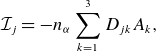 \begin{align} \mathcal{I}_j = - n_\alpha \sum \limits _{k=1}^3 D_{jk}A_k, \end{align}
to thermodynamic fluxes $\mathcal{I}_j$
defined via particle,
$\mathcal{I}_j$
defined via particle, $\Gamma _\alpha$
, and energy,
$\Gamma _\alpha$
, and energy, $Q_\alpha$
, flux density and parallel flow velocity
$Q_\alpha$
, flux density and parallel flow velocity $V_{\parallel \alpha }$
as follows:
$V_{\parallel \alpha }$
as follows:
 \begin{align} \mathcal{I}_1=\Gamma _\alpha, \qquad \mathcal{I}_2=\frac {Q_\alpha }{T_\alpha }, \qquad \mathcal{I}_3=n_\alpha \left \langle V_{\parallel \alpha } B\right \rangle . \end{align}
These transport coefficients are obtained by energy convolution of mono-energetic coefficients (Beidler et al. Reference Beidler2011) $\bar D_{jk}$
with a local Maxwellian
$\bar D_{jk}$
with a local Maxwellian
 \begin{align} D_{jk} = \frac {2}{\sqrt {\pi }}\int \limits _0^\infty \textrm { d} z \sqrt {z}\textrm { e}^{-z} \bar D_{jk}. \end{align}
Presenting neoclassical flux surface averages in the form of field line averages explicitly given in field aligned variables by
 \begin{align} \langle a \rangle = \lim \limits _{\varphi _N\rightarrow \infty } \left (\int \limits _{\varphi _0}^{\varphi _N}\frac {\textrm { d} \varphi }{B^\varphi }\right )^{-1} \int \limits _{\varphi _0}^{\varphi _N}\frac {\textrm { d} \varphi }{B^\varphi } a, \end{align}
the mono-energetic coefficients are given by
 \begin{align} \bar D_{jk} =v \lim \limits _{\varphi _N\rightarrow \infty } \left (\int \limits _{\varphi _0}^{\varphi _N}\frac {\textrm { d} \varphi }{B^\varphi }\!\right )^{-1} \frac {1}{4} \sum _{\sigma =\pm 1}\int \limits _{\varphi _0}^{\varphi _N}\textrm { d} \varphi\! \int \limits _0^{1/B}\textrm { d} \eta \; s_{(j)}^\dagger g_{(k)} \equiv v \lim \limits _{\varphi _N\rightarrow \infty } \int \limits _{\Omega _N}\! \textrm { d}\Omega \; s_{(j)}^\dagger g_{(k)}, \end{align}
where
 \begin{align} a^\dagger (\varphi, \eta, \sigma ) = a(\varphi, \eta, -\sigma ). \end{align}
Definitions of thermodynamic forces and fluxes and, respectively, of diffusion coefficients (2.9) here are the same as in Kernbichler et al. (Reference Kernbichler, Kasilov, Kapper, Martitsch, Nemov and Heyn2016) and coincide with those of Beidler et al. (Reference Beidler2011) for the reference field $B_0=1$
except for the sign of
$B_0=1$
except for the sign of $A_3$
. The sign convention used here results in a simple Onsager symmetry for all transport coefficients,
$A_3$
. The sign convention used here results in a simple Onsager symmetry for all transport coefficients, $D_{jk}=D_{kj}$
, but negative coefficient
$D_{jk}=D_{kj}$
, but negative coefficient $D_{33}$
corresponding to plasma conductivity.
$D_{33}$
corresponding to plasma conductivity.
For the present analysis, we solve the kinetic equation on the rational surface using a ‘representative’ field line where necessary conditions valid for the irrational flux surface are fulfilled. The flux surface average (2.10) at the irrational surface corresponds then to the limit of the series of representative field lines closed after $N$
turns at respective rational surfaces,
$N$
turns at respective rational surfaces, $r=r_N,\;\mbox{where}\; \iota(r_N)=M/N$
, which converge to the irrational surface,
$r=r_N,\;\mbox{where}\; \iota(r_N)=M/N$
, which converge to the irrational surface, $\lim \limits _{N \rightarrow \infty }\iota (r_N) = \iota (r)$
. The requested condition is Liouville’s theorem, which states that the integral over any closed surface of the normal component of the guiding center velocity multiplied by the phase space Jacobian is zero for fixed total energy and the perpendicular adiabatic invariant used as phase space variables. For the magnetic surface with constant electrostatic potential, this means
$\lim \limits _{N \rightarrow \infty }\iota (r_N) = \iota (r)$
. The requested condition is Liouville’s theorem, which states that the integral over any closed surface of the normal component of the guiding center velocity multiplied by the phase space Jacobian is zero for fixed total energy and the perpendicular adiabatic invariant used as phase space variables. For the magnetic surface with constant electrostatic potential, this means $\left \langle B v_g^r / v_\parallel \right \rangle =0$
, where the surface integration is performed over regions where
$\left \langle B v_g^r / v_\parallel \right \rangle =0$
, where the surface integration is performed over regions where $v_\parallel ^2 = v^2 (1-\eta B)\geqslant 0$
keeping invariants
$v_\parallel ^2 = v^2 (1-\eta B)\geqslant 0$
keeping invariants $z$
and
$z$
and $\eta$
constant. The field line average form (2.10) of Liouville’s theorem results in
$\eta$
constant. The field line average form (2.10) of Liouville’s theorem results in
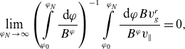 \begin{align} \lim \limits _{\varphi _N\rightarrow \infty } \left (\int \limits _{\varphi _0}^{\varphi _N}\frac {\textrm { d} \varphi }{B^\varphi }\right )^{-1} \int \limits _{\varphi _0}^{\varphi _N}\frac {\textrm { d} \varphi B v_g^r}{B^\varphi v_\parallel }=0, \end{align}
for passing particles and in
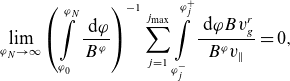 \begin{align} \lim \limits _{\varphi _N\rightarrow \infty } \left (\int \limits _{\varphi _0}^{\varphi _N}\frac {\textrm { d} \varphi }{B^\varphi }\right )^{-1} \sum \limits _{j=1}^{j_{\textrm{max}}}\int \limits _{\varphi _j^-}^{\varphi _j^+}\frac {\textrm { d} \varphi B v_g^r}{B^\varphi v_\parallel }=0, \end{align}
for trapped particles, where $\varphi _j^-(\eta )$
and
$\varphi _j^-(\eta )$
and $\varphi _j^+(\eta )$
are the left and right turning points, being solutions to
$\varphi _j^+(\eta )$
are the left and right turning points, being solutions to $\eta B(\varphi ^\pm _j)=1$
, index
$\eta B(\varphi ^\pm _j)=1$
, index $j$
enumerates local magnetic field maxima
$j$
enumerates local magnetic field maxima $B(\varphi _j)$
fulfilling
$B(\varphi _j)$
fulfilling $B(\varphi _j)\eta \gt 1$
so that turning points are contained between maximum points
$B(\varphi _j)\eta \gt 1$
so that turning points are contained between maximum points $\varphi _{j}$
and
$\varphi _{j}$
and $\varphi _{j+1}$
. The upper summation limit
$\varphi _{j+1}$
. The upper summation limit $j_{\textrm{max}}=j_{\textrm{max}}(\eta, N)$
is the total number of such maxima between
$j_{\textrm{max}}=j_{\textrm{max}}(\eta, N)$
is the total number of such maxima between $\varphi _0$
and
$\varphi _0$
and $\varphi _N$
. For the “representative” closed field line with
$\varphi _N$
. For the “representative” closed field line with $\varphi _0$
at the largest maximum we require that conditions (2.13) and (2.14) are fulfilled exactly for finite
$\varphi _0$
at the largest maximum we require that conditions (2.13) and (2.14) are fulfilled exactly for finite $\varphi _N$
, i.e.
$\varphi _N$
, i.e.
 \begin{align} \int \limits _{\varphi _0}^{\varphi _N} \textrm { d} \varphi \; s_{(1)}=0, \qquad \sum \limits _{j=1}^{j_{\textrm{max}}}\int \limits _{\varphi _j^-}^{\varphi _j^+} \textrm { d} \varphi \; s_{(1)}=0, \end{align}
for passing and trapped particles, respectively (see (2.4)). We will call these conditions “quasi-Liouville’s theorem”. In the devices with stellarator symmetry conditions (2.15) are satisfied for closed field lines passing through the magnetic field symmetry point $\varphi _{\text{sts}}$
which is obvious due to anti-symmetry of the geodesic curvature (and, respectively, of
$\varphi _{\text{sts}}$
which is obvious due to anti-symmetry of the geodesic curvature (and, respectively, of $v_g^r$
and
$v_g^r$
and $s_{(1)}$
) with respect to this point,
$s_{(1)}$
) with respect to this point, $s_{(1)}(2\varphi _{\text{sts}}-\varphi )=-s_{(1)}(\varphi )$
. Restricting our analysis to such devices with a single global maximum per field period, the reference field line is then the one starting from the global maximum, which must be located at one of (at least two possible) symmetry points
$s_{(1)}(2\varphi _{\text{sts}}-\varphi )=-s_{(1)}(\varphi )$
. Restricting our analysis to such devices with a single global maximum per field period, the reference field line is then the one starting from the global maximum, which must be located at one of (at least two possible) symmetry points $\varphi _0 \in \varphi _{\text{sts}}$
.
$\varphi _0 \in \varphi _{\text{sts}}$
.
Representing flux surface averages (2.10) and (2.11) by the same expressions without the limit $\varphi _N\rightarrow \infty$
, one can check that so defined mono-energetic coefficients stay Onsager-symmetric. Namely, replacing source terms in (2.11) via equation (2.3), integrating by parts and using the periodicity of the distribution in the passing region,
$\varphi _N\rightarrow \infty$
, one can check that so defined mono-energetic coefficients stay Onsager-symmetric. Namely, replacing source terms in (2.11) via equation (2.3), integrating by parts and using the periodicity of the distribution in the passing region, $g(\varphi _0,\eta, \sigma )=g(\varphi _N,\eta, \sigma )$
and its continuity at the turning points in the trapped region,
$g(\varphi _0,\eta, \sigma )=g(\varphi _N,\eta, \sigma )$
and its continuity at the turning points in the trapped region, $g(\varphi _j^\pm, \eta, 1)=g(\varphi _j^\pm, \eta, -1)$
, we get
$g(\varphi _j^\pm, \eta, 1)=g(\varphi _j^\pm, \eta, -1)$
, we get
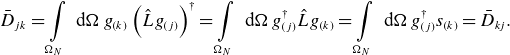 \begin{eqnarray} \bar D_{jk} = \int \limits _{\Omega _N} \textrm { d} \Omega \; g_{(k)} \left (\hat L g_{(j)}\right )^\dagger = \int \limits _{\Omega _N} \textrm { d} \Omega \; g^\dagger _{(j)} \hat L g_{(k)} = \int \limits _{\Omega _N} \textrm { d} \Omega \; g_{(j)}^\dagger s_{(k)} = \bar D_{kj}. \end{eqnarray}
Thus, we can either compute the bootstrap coefficient $\bar D_{31}$
solving the direct problem driven by
$\bar D_{31}$
solving the direct problem driven by $s_{(1)}$
or use its equality to the Ware-pinch coefficient
$s_{(1)}$
or use its equality to the Ware-pinch coefficient $\bar D_{13}$
resulting from the adjoint problem driven by
$\bar D_{13}$
resulting from the adjoint problem driven by $s_{(3)}$
.
$s_{(3)}$
.
2.2. Collisionless asymptotic solutions
Omitting the drive index $(k)$
, asymptotic solutions of (2.3) in the long mean free path limit
$(k)$
, asymptotic solutions of (2.3) in the long mean free path limit $l_c \rightarrow \infty$
follow from the standard procedure where the normalized distribution function is looked for in the form of the series expansion in
$l_c \rightarrow \infty$
follow from the standard procedure where the normalized distribution function is looked for in the form of the series expansion in $l_c^{-1}$
 \begin{align} g(\varphi, \eta, \sigma ) = g_{-1}(\eta, \sigma )+g_0(\varphi, \eta, \sigma )+g_1(\varphi, \eta, \sigma )+\ldots, \end{align}
where the leading-order term $g_{-1}$
is independent of
$g_{-1}$
is independent of $\varphi$
, and corrections satisfy
$\varphi$
, and corrections satisfy
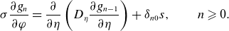 \begin{align} \sigma \frac {\partial g_n}{\partial \varphi } =\frac {\partial }{\partial \eta }\left (D_\eta \frac {\partial g_{n-1}}{\partial \eta }\right )+\delta _{n0}s, \qquad n \geqslant 0. \end{align}
Equation (2.18) is integrated to
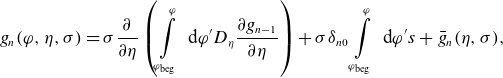 \begin{align} g_n(\varphi, \eta, \sigma ) =\sigma \frac {\partial }{\partial \eta } \left (\int \limits _{\varphi _{ \textrm{beg}}}^\varphi \textrm { d} \varphi ^\prime D_\eta \frac {\partial g_{n-1}}{\partial \eta }\right ) +\sigma \delta _{n0} \int \limits _{\varphi _{\textrm{beg}}}^\varphi \textrm { d} \varphi ^\prime s+\bar g_n(\eta, \sigma ), \end{align}
where $\varphi _{\textrm{beg}}=\varphi _j^-(\eta )$
for trapped particles and
$\varphi _{\textrm{beg}}=\varphi _j^-(\eta )$
for trapped particles and $\varphi _{\textrm{beg}}=\varphi _0$
for passing, and we require that each of
$\varphi _{\textrm{beg}}=\varphi _0$
for passing, and we require that each of $g_n$
is continuous at the periodic boundary and at the turning points. Continuity at
$g_n$
is continuous at the periodic boundary and at the turning points. Continuity at $\varphi =\varphi _j^-$
means that
$\varphi =\varphi _j^-$
means that $\bar g_n$
is an even function of
$\bar g_n$
is an even function of $\sigma$
in the trapped region,
$\sigma$
in the trapped region, $\bar g_n=\bar g_n(\eta )$
, while continuity at the periodic boundary in the passing region and at
$\bar g_n=\bar g_n(\eta )$
, while continuity at the periodic boundary in the passing region and at $\varphi =\varphi _j^+$
in the trapped region results in an equation for the integration constant
$\varphi =\varphi _j^+$
in the trapped region results in an equation for the integration constant $\bar g_{n-1}$
(solubility constraint for
$\bar g_{n-1}$
(solubility constraint for $g_n$
). The leading-order constraint for
$g_n$
). The leading-order constraint for $g_0$
gives a bounce-averaged equation for
$g_0$
gives a bounce-averaged equation for $g_{-1}$
 \begin{align} \sum \limits _{\sigma =\pm 1}^{\textrm{trapped}}\left (\frac {\partial }{\partial \eta } \left ( \frac {\partial g_{-1}}{\partial \eta } \int \limits _{\varphi _{\textrm{beg}}}^{\varphi _{\textrm{end}}} \textrm { d} \varphi ^\prime D_\eta \right ) +\int \limits _{\varphi _{\textrm{beg}}}^{\varphi _{\textrm{end}}} \textrm { d} \varphi ^\prime s\right )=0, \end{align}
where $\varphi _{\textrm{end}}=\varphi _j^+(\eta )$
for trapped particles and
$\varphi _{\textrm{end}}=\varphi _j^+(\eta )$
for trapped particles and $\varphi _{\textrm{end}}=\varphi _N$
for passing, and the sum
$\varphi _{\textrm{end}}=\varphi _N$
for passing, and the sum $\sum \limits _{\sigma =\pm 1}^{\textrm{trapped}}$
is taken for trapped particles only. Higher-order constraints result in equations for integration constants
$\sum \limits _{\sigma =\pm 1}^{\textrm{trapped}}$
is taken for trapped particles only. Higher-order constraints result in equations for integration constants $\bar g_n$
 \begin{align} \sum \limits _{\sigma =\pm 1}^{\textrm{trapped}} \frac {\partial }{\partial \eta } \left ( \frac {\partial \bar g_n}{\partial \eta } \int \limits _{\varphi _{\textrm{beg}}}^{\varphi _{\textrm{end}}} \textrm { d} \varphi ^\prime D_\eta + \int \limits _{\varphi _{\textrm{beg}}}^{\varphi _{\textrm{end}}} \textrm { d} \varphi ^\prime D_\eta \frac {\partial (g_{n}-\bar g_n)}{\partial \eta }\right ) = 0, \qquad n \geqslant 0, \end{align}
where $g_n-\bar g_n$
is determined by
$g_n-\bar g_n$
is determined by $g_{n-1}$
via (2.19).
$g_{n-1}$
via (2.19).
Since boundary conditions for the collisional flux in velocity space restrict only the whole solution (2.17), we have a freedom for setting boundary conditions for individual expansion terms. Thus, we can require that this flux is produced by $g_{-1}$
only
$g_{-1}$
only
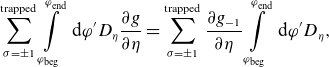 \begin{align} \sum \limits _{\sigma =\pm 1}^{\textrm{trapped}}\int \limits _{\varphi _{\textrm{beg}}}^{\varphi _{\textrm{end}}} \textrm { d} \varphi ^\prime D_\eta \frac {\partial g}{\partial \eta } = \sum \limits _{\sigma =\pm 1}^{\textrm{trapped}}\frac {\partial g_{-1}}{\partial \eta } \int \limits _{\varphi _{\textrm{beg}}}^{\varphi _{\textrm{end}}} \textrm { d} \varphi ^\prime D_\eta, \end{align}
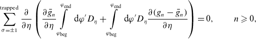
while the corrections carry no flux so that (2.21) is integrated to
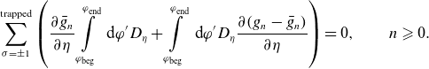 \begin{align} \sum \limits _{\sigma =\pm 1}^{\textrm{trapped}} \left ( \frac {\partial \bar g_n}{\partial \eta } \int \limits _{\varphi _{\textrm{beg}}}^{\varphi _{\textrm{end}}} \textrm { d} \varphi ^\prime D_\eta + \int \limits _{\varphi _{\textrm{beg}}}^{\varphi _{\textrm{end}}} \textrm { d} \varphi ^\prime D_\eta \frac {\partial (g_{n}-\bar g_n)}{\partial \eta }\right ) = 0, \qquad n \geqslant 0. \end{align}
We apply this ansatz separately to the direct problem driven by source $s_{(1)}$
and to the adjoint problem driven by source
$s_{(1)}$
and to the adjoint problem driven by source $s_{(3)}$
.
$s_{(3)}$
.
2.2.1. Direct problem
Due to the first condition (2.15), the bounce-averaged equation (2.20) for passing particles is homogeneous
 \begin{align} \frac {\partial }{\partial \eta } \left (\frac {\partial g_{-1}}{\partial \eta }\int \limits _{\varphi _0}^{\varphi _N} \textrm { d} \varphi ^\prime D_\eta \right )=0. \end{align}
Integrating it once and applying the boundary condition $\partial g_{-1} / \partial \eta = 0$
at the strongly passing boundary
$\partial g_{-1} / \partial \eta = 0$
at the strongly passing boundary $\eta =0$
we get
$\eta =0$
we get $g_{-1}=\text {const.}$
in the passing region. Since
$g_{-1}=\text {const.}$
in the passing region. Since $g_{-1}$
is continuous at the global maximum point
$g_{-1}$
is continuous at the global maximum point $\varphi =\varphi _0$
at the trapped–passing boundary
$\varphi =\varphi _0$
at the trapped–passing boundary $\eta =1/B_{\textrm{max}}$
, the function
$\eta =1/B_{\textrm{max}}$
, the function $g_{-1}$
can only be even. Since any constant satisfies the homogeneous mono-energetic equation in the whole phase space making no contribution to transport coefficients but only re-defining the moments of equilibrium Maxwellian, we fix
$g_{-1}$
can only be even. Since any constant satisfies the homogeneous mono-energetic equation in the whole phase space making no contribution to transport coefficients but only re-defining the moments of equilibrium Maxwellian, we fix $g_{-1}=0$
in the passing region. In the trapped region, (2.20) is
$g_{-1}=0$
in the passing region. In the trapped region, (2.20) is
 \begin{align} \frac {\partial }{\partial \eta } \left (\frac {\eta I_j}{l_c} \frac {\partial g_{-1}}{\partial \eta }+H_j \right )=0, \end{align}
where we denoted
 \begin{align} I_j(\eta ) = \int \limits _{\varphi _j^-(\eta )}^{\varphi _j^+(\eta )} \textrm { d} \varphi \frac {|\lambda |}{B^\varphi }, \qquad H_j(\eta ) = \int \limits _{\varphi _j^-(\eta )}^{\varphi _j^+(\eta )} \textrm { d} \varphi H^\prime _\varphi, \end{align}
see definitions (2.3)–(2.5). Since $\partial g_{-1} /\partial \eta =0$
at the bottoms of local magnetic wells
$\partial g_{-1} /\partial \eta =0$
at the bottoms of local magnetic wells $\eta =1/B_{\textrm{min}}^{\textrm{loc}}$
where
$\eta =1/B_{\textrm{min}}^{\textrm{loc}}$
where $H_j=0$
due to
$H_j=0$
due to $\varphi _j^+=\varphi _j^-$
we can integrate (2.25) to
$\varphi _j^+=\varphi _j^-$
we can integrate (2.25) to
 \begin{align} \frac {\partial g_{-1}(\eta )}{\partial \eta } =-\frac {l_c H_j}{\eta I_j}. \end{align}
This solution automatically satisfies collisional flux conservation relations in all boundary layers separating different trapped particle classes
 \begin{align} \left [I_j\frac {\partial g^{(j)}_{-1}}{\partial \eta }\right ]_{\eta =\eta _c-o} = \left [I_j\frac {\partial g^{(j)}_{-1}}{\partial \eta }\right ]_{\eta =\eta _c+o} + \left [I_{j+1}\frac {\partial g^{(j+1)}_{-1}}{\partial \eta }\right ]_{\eta =\eta _c+o}, \end{align}
where $\eta _c=1/B_{\textrm{max}}^{\textrm{loc}}$
, see figure 1,
$\eta _c=1/B_{\textrm{max}}^{\textrm{loc}}$
, see figure 1, $o$
denotes an infinitesimal number and the superscript
$o$
denotes an infinitesimal number and the superscript $(j)$
on
$(j)$
on $g_{-1}$
denotes particle type trapped between the reflection points
$g_{-1}$
denotes particle type trapped between the reflection points $\varphi _j^\pm$
. Derivative (2.27) satisfies also the flux conservation through the trapped–passing boundary
$\varphi _j^\pm$
. Derivative (2.27) satisfies also the flux conservation through the trapped–passing boundary $\eta =\eta _b$
turning there to zero, because only a single type of trapped particles exists near this boundary, and
$\eta =\eta _b$
turning there to zero, because only a single type of trapped particles exists near this boundary, and $H_1(\eta _b+o)=0$
follows then from the second condition (2.15).
$H_1(\eta _b+o)=0$
follows then from the second condition (2.15).
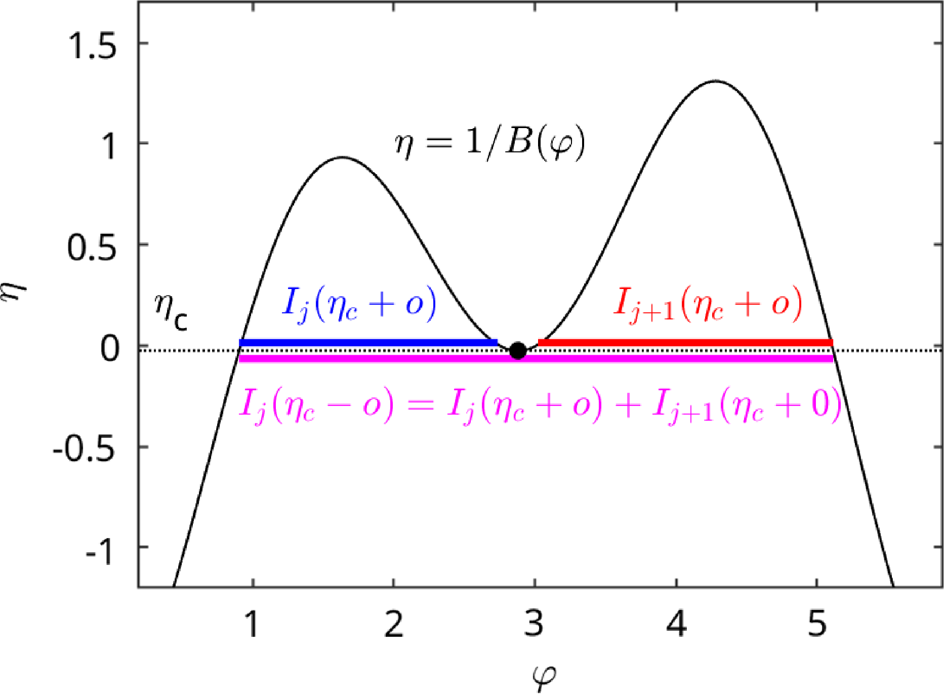
Figure 1. Example of class-transition boundary introduced by local field maximum $B_{\textrm{max}}^{\textrm{loc}}$
(black dot) where three types of trapped particles meet (two “single-trapped” and one “double-trapped”). Boundary conditions (2.28) are fulfilled by (2.27) due
$B_{\textrm{max}}^{\textrm{loc}}$
(black dot) where three types of trapped particles meet (two “single-trapped” and one “double-trapped”). Boundary conditions (2.28) are fulfilled by (2.27) due $H_j(\eta _c-o)=H_j(\eta _c+o)+H_{j+1}(\eta _c+o)$
.
$H_j(\eta _c-o)=H_j(\eta _c+o)+H_{j+1}(\eta _c+o)$
.
Solution (2.27) is sufficient for the computation of the effective ripple (Nemov et al. Reference Nemov, Kasilov, Kernbichler and Heyn1999) $\varepsilon _{\text{eff}}$
which determines device geometry effect on the mono-energetic diffusion coefficient
$\varepsilon _{\text{eff}}$
which determines device geometry effect on the mono-energetic diffusion coefficient $\bar D_{11}$
(and all other
$\bar D_{11}$
(and all other $\bar D_{jk}$
for
$\bar D_{jk}$
for $j,k \leqslant 2$
trivially related to
$j,k \leqslant 2$
trivially related to $\bar D_{11}$
). Substituting in (2.11)
$\bar D_{11}$
). Substituting in (2.11) $g_{(1)}=g_{-1}$
and
$g_{(1)}=g_{-1}$
and $s_{(1)}$
via (2.4), integrating the result by parts over
$s_{(1)}$
via (2.4), integrating the result by parts over $\eta$
and using the continuity of
$\eta$
and using the continuity of $g_{-1}$
through all boundary layers, changing the integration order over
$g_{-1}$
through all boundary layers, changing the integration order over $\varphi$
and
$\varphi$
and $\eta$
results in
$\eta$
results in
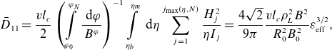 \begin{align} \bar D_{11} = \frac {v l_c}{2} \left (\int \limits _{\varphi _0}^{\varphi _N}\frac {\textrm { d} \varphi }{B^\varphi }\right )^{-1} \int \limits _{\eta _b}^{\eta _m}\textrm { d} \eta \sum \limits _{j=1}^{j_{\textrm{max}}(\eta, N)} \frac {H_j^2}{\eta I_j} =\frac {4\sqrt {2}}{9\pi }\frac {v l_c \rho _L^2 B^2}{R_0^2 B_0^2}\varepsilon _{\text{eff}}^{3/2}, \end{align}
where $\eta _b=1/B_{\textrm{max}}$
and
$\eta _b=1/B_{\textrm{max}}$
and $\eta _m=1/B_{\textrm{min}}$
are defined by global field maximum and minimum, respectively. The last equality (2.29) where
$\eta _m=1/B_{\textrm{min}}$
are defined by global field maximum and minimum, respectively. The last equality (2.29) where $R_0$
and
$R_0$
and $B_0$
are reference values of major radius and magnetic field, respectively, defines
$B_0$
are reference values of major radius and magnetic field, respectively, defines $\varepsilon _{\text{eff}}^{3/2}$
in the same way as equation (29) of Nemov et al. (Reference Nemov, Kasilov, Kernbichler and Heyn1999), where quantities
$\varepsilon _{\text{eff}}^{3/2}$
in the same way as equation (29) of Nemov et al. (Reference Nemov, Kasilov, Kernbichler and Heyn1999), where quantities $\hat I_j(b^\prime )$
and
$\hat I_j(b^\prime )$
and $\hat H_j(b^\prime )$
are related to the present notation by
$\hat H_j(b^\prime )$
are related to the present notation by $\hat I_j = I_j$
and
$\hat I_j = I_j$
and $\hat H_j = 3 B_0^{3/2}\eta ^{1/2}(\rho _L B)^{-1} H_j$
with
$\hat H_j = 3 B_0^{3/2}\eta ^{1/2}(\rho _L B)^{-1} H_j$
with $b^\prime =(B_0\eta )^{-1}$
.
$b^\prime =(B_0\eta )^{-1}$
.
For the next-order correction $g_0$
, we notice that the first two terms in the right-hand side of (2.19) are odd in
$g_0$
, we notice that the first two terms in the right-hand side of (2.19) are odd in $\sigma$
. Therefore, in the trapped particle region, equation (2.23) for the integration constant (which can only be even there) is homogeneous, resulting in
$\sigma$
. Therefore, in the trapped particle region, equation (2.23) for the integration constant (which can only be even there) is homogeneous, resulting in $\bar g_0=\text {const}$
. Due to the continuity of the distribution function across the trapped–passing boundary, the integration constant in the passing region is the same. We can again absorb this constant into the equilibrium Maxwellian, as we have already done in the previous order when setting
$\bar g_0=\text {const}$
. Due to the continuity of the distribution function across the trapped–passing boundary, the integration constant in the passing region is the same. We can again absorb this constant into the equilibrium Maxwellian, as we have already done in the previous order when setting $g_{-1}=0$
in the passing region. Thus, substituting in (2.19) the derivative
$g_{-1}=0$
in the passing region. Thus, substituting in (2.19) the derivative $\partial g_{-1}/\partial \eta$
via (2.27) and the source
$\partial g_{-1}/\partial \eta$
via (2.27) and the source $s=s_{(1)}$
via (2.4) and (2.5) we get explicitly
$s=s_{(1)}$
via (2.4) and (2.5) we get explicitly
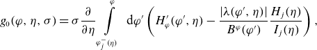 \begin{align} g_0(\varphi, \eta, \sigma ) =\sigma \frac {\partial }{\partial \eta } \int \limits _{\varphi _j^-(\eta )}^\varphi \textrm { d} \varphi ^\prime \left (H_\varphi ^\prime (\varphi ^\prime, \eta ) -\frac {|\lambda (\varphi ^\prime, \eta )| }{B^\varphi (\varphi ^\prime )} \frac {H_j(\eta )}{I_j(\eta )} \right ), \end{align}
where we have exchanged the derivative over $\eta$
with integration in the first term using
$\eta$
with integration in the first term using $H_\varphi ^\prime (\varphi _j^-(\eta ),\eta )=0$
. It should be noted now that the integral over
$H_\varphi ^\prime (\varphi _j^-(\eta ),\eta )=0$
. It should be noted now that the integral over $\varphi ^\prime$
is a discontinuous function of
$\varphi ^\prime$
is a discontinuous function of $\eta$
at the boundaries between classes
$\eta$
at the boundaries between classes $\eta =\eta _c$
where either
$\eta =\eta _c$
where either $\varphi _j^-(\eta )$
or
$\varphi _j^-(\eta )$
or $\varphi _j^+(\eta )$
jumps. Respectively, the function
$\varphi _j^+(\eta )$
jumps. Respectively, the function $g_0$
contains a
$g_0$
contains a $\delta$
-function
$\delta$
-function $\delta (\eta -\eta _c)$
, which is required by particle conservation in the boundary layer. Namely, integrating (2.3) over
$\delta (\eta -\eta _c)$
, which is required by particle conservation in the boundary layer. Namely, integrating (2.3) over $\eta$
across the boundary, we get
$\eta$
across the boundary, we get
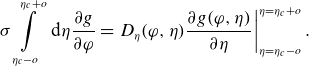 \begin{align} \sigma \int \limits _{\eta _c-o}^{\eta _c+o}\textrm { d} \eta \frac {\partial g}{\partial \varphi }= \left . D_\eta (\varphi, \eta )\frac {\partial g(\varphi, \eta )}{\partial \eta }\right |_{\eta =\eta _c-o}^{\eta =\eta _c+o}. \end{align}
Substituting here $g=g_{-1}+g_0$
and ignoring
$g=g_{-1}+g_0$
and ignoring $g_0$
on the right-hand side where its contribution is linear in collisionality we get
$g_0$
on the right-hand side where its contribution is linear in collisionality we get
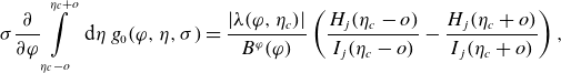 \begin{align} \sigma \frac {\partial }{\partial \varphi } \int \limits _{\eta _c-o}^{\eta _c+o}\textrm { d} \eta \; g_0(\varphi, \eta, \sigma ) = \frac {|\lambda (\varphi, \eta _c)|}{B^\varphi (\varphi )} \left (\frac {H_j(\eta _c-o)}{I_j(\eta _c-o)} - \frac {H_j(\eta _c+o)}{I_j(\eta _c+o)}\right ), \end{align}
which is an identity for $g_0$
in the form (2.30).
$g_0$
in the form (2.30).
In the passing region where $g_{-1}=0$
, (2.19) results in
$g_{-1}=0$
, (2.19) results in
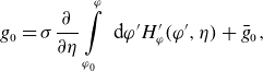 \begin{align} g_0 = \sigma \frac {\partial }{\partial \eta } \int \limits _{\varphi _0}^\varphi \textrm { d} \varphi ^\prime H_\varphi ^\prime (\varphi ^\prime, \eta ) + \bar g_0, \end{align}
where
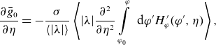 \begin{align} \frac {\partial \bar g_0}{\partial \eta }= -\frac {\sigma }{\langle |\lambda | \rangle } \left \langle |\lambda | \frac {\partial ^2}{\partial \eta ^2} \int \limits _{\varphi _0}^\varphi \textrm { d} \varphi ^\prime H_\varphi ^\prime (\varphi ^\prime, \eta ) \right \rangle, \end{align}
follows from (2.23) and $\langle \ldots \rangle$
denotes a field line average (flux surface average (2.10) with
$\langle \ldots \rangle$
denotes a field line average (flux surface average (2.10) with $\varphi _N$
kept finite). This derivative has an integrable singularity at the trapped–passing boundary,
$\varphi _N$
kept finite). This derivative has an integrable singularity at the trapped–passing boundary, $\partial \bar g_0 /\partial \eta \propto (\eta _b-\eta )^{-1/2}$
which follows from
$\partial \bar g_0 /\partial \eta \propto (\eta _b-\eta )^{-1/2}$
which follows from $|\nabla r| k_G \propto (\varphi -\varphi _0)$
near the global maximum
$|\nabla r| k_G \propto (\varphi -\varphi _0)$
near the global maximum $\varphi =\varphi _0$
(and
$\varphi =\varphi _0$
(and $\varphi =\varphi _N$
since the innermost integral is a single-valued (periodic) function of
$\varphi =\varphi _N$
since the innermost integral is a single-valued (periodic) function of $\varphi$
on the closed field line). Therefore,
$\varphi$
on the closed field line). Therefore, $\bar g_0$
is continuous at the trapped–passing boundary, where it is connected to
$\bar g_0$
is continuous at the trapped–passing boundary, where it is connected to $\bar g_0=0$
in the trapped region. Moreover, the derivative of the full solution
$\bar g_0=0$
in the trapped region. Moreover, the derivative of the full solution $\partial g_0 / \partial \eta$
has no singularity at this boundary (in contrast to
$\partial g_0 / \partial \eta$
has no singularity at this boundary (in contrast to $\partial \bar g_0 / \partial \eta$
). One can also check that this derivative does not depend on the lower integration limit
$\partial \bar g_0 / \partial \eta$
). One can also check that this derivative does not depend on the lower integration limit $\varphi _0$
in (2.33) and (2.34) which, therefore, needs not to be the global maximum point.
$\varphi _0$
in (2.33) and (2.34) which, therefore, needs not to be the global maximum point.
We can formally combine expressions (2.30) and (2.33) into
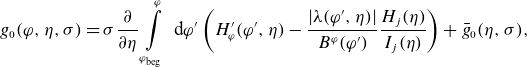 \begin{align} g_0(\varphi, \eta, \sigma ) =\sigma \frac {\partial }{\partial \eta } \int \limits _{\varphi _{\textrm{beg}}}^\varphi \textrm { d} \varphi ^\prime \left (H_\varphi ^\prime (\varphi ^\prime, \eta ) -\frac {|\lambda (\varphi ^\prime, \eta )| }{B^\varphi (\varphi ^\prime )} \frac {H_j(\eta )}{I_j(\eta )} \right )+\bar g_0(\eta, \sigma ), \end{align}
valid for the whole phase space with $I_j=I_0$
and
$I_j=I_0$
and $H_j=H_0=0$
in the passing region where they are given by (2.26) with the limits
$H_j=H_0=0$
in the passing region where they are given by (2.26) with the limits $\varphi _0$
and
$\varphi _0$
and $\varphi _N$
instead of
$\varphi _N$
instead of $\varphi _j^\pm$
. Due to the linear scaling of
$\varphi _j^\pm$
. Due to the linear scaling of $g_0$
with velocity module
$g_0$
with velocity module $v$
, we can evaluate energy integral in the expression for the parallel current density of the
$v$
, we can evaluate energy integral in the expression for the parallel current density of the $\alpha$
species substituting in (2.1)
$\alpha$
species substituting in (2.1) $g=g_0$
which is the only term contributing in the leading order
$g=g_0$
which is the only term contributing in the leading order
 \begin{align} j_{\parallel \alpha }= e_\alpha \int \textrm { d}^3 v v_\parallel (f-f_M)= C_\alpha B \sum \limits _{\sigma =\pm 1}\sigma \int \limits _0^{1/B}\textrm { d}\eta \; g_0, \end{align}
where
 \begin{align} C_\alpha = \frac {3 c}{4 B\rho _L}\left (\frac {\partial p_\alpha }{\partial r}-e_\alpha n_\alpha E_r\right ), \qquad p_\alpha = n_\alpha T_\alpha, \end{align}
and we omitted the inductive current by setting $A_3=0$
. Since
$A_3=0$
. Since $g_0/\rho _L$
is independent of particle species, total current density is independent of
$g_0/\rho _L$
is independent of particle species, total current density is independent of $E_r$
in quasi-neutral plasmas,
$E_r$
in quasi-neutral plasmas,
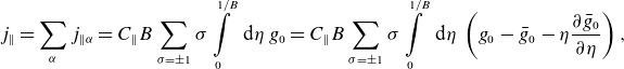 \begin{align} j_{\parallel }= \sum _\alpha j_{\parallel \alpha }= C_\parallel B \sum \limits _{\sigma =\pm 1}\sigma \int \limits _0^{1/B}\textrm { d}\eta \; g_0 =C_\parallel B \sum \limits _{\sigma =\pm 1}\sigma \int \limits _0^{1/B}\textrm { d}\eta \; \left (g_0 - \bar g_0 - \eta \frac {\partial \bar g_0}{\partial \eta }\right ), \end{align}
where
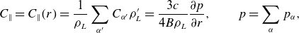 \begin{align} C_\parallel = C_\parallel (r) = \frac {1}{\rho _L}\sum _{\alpha ^\prime } C_{\alpha ^\prime } \rho _L^\prime = \frac {3 c}{4 B \rho _L} \frac {\partial p}{\partial r}, \qquad p=\sum _\alpha p_\alpha, \end{align}
where $\rho _L^\prime$
denotes the Larmor radius of
$\rho _L^\prime$
denotes the Larmor radius of $\alpha ^\prime$
species, and we used the condition
$\alpha ^\prime$
species, and we used the condition $\bar g_0=0$
at the boundary
$\bar g_0=0$
at the boundary $\eta =1/B$
when integrating by parts in the last expression (2.38). According to (2.35), the term
$\eta =1/B$
when integrating by parts in the last expression (2.38). According to (2.35), the term $g_0-\bar g_0$
is a derivative which contributes only at the lower limit
$g_0-\bar g_0$
is a derivative which contributes only at the lower limit $\eta =0$
where using explicitly (2.5) one gets parallel equilibrium current density as
$\eta =0$
where using explicitly (2.5) one gets parallel equilibrium current density as
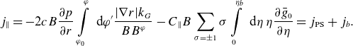 \begin{align} j_{\parallel } = - 2 c B \frac {\partial p}{\partial r}\int \limits _{\varphi _0}^{\varphi } \textrm { d} \varphi ^\prime \frac {|\nabla r| k_G}{B B^\varphi } -C_\parallel B \sum \limits _{\sigma =\pm 1}\sigma \int \limits _0^{\eta _b}\textrm { d}\eta \; \eta \frac {\partial \bar g_0}{\partial \eta }=j_{\text {PS}}+j_b. \end{align}
Here, as well as in (2.34), the point $\varphi _0$
must be at a global maximum because integration over
$\varphi _0$
must be at a global maximum because integration over $\eta$
in the first term required the continuity of
$\eta$
in the first term required the continuity of $\varphi _{\textrm{beg}}$
at the trapped–passing boundary. Equation (2.40) naturally agrees with the ideal magnetohydrodynamic radial force balance which determines the Pfirsch–Schlüter current density
$\varphi _{\textrm{beg}}$
at the trapped–passing boundary. Equation (2.40) naturally agrees with the ideal magnetohydrodynamic radial force balance which determines the Pfirsch–Schlüter current density $j_{\text {PS}}$
up to the arbitrary constant times
$j_{\text {PS}}$
up to the arbitrary constant times $B$
. Due to quasi-Liouville’s theorem (2.15), the current density (2.40) is periodic,
$B$
. Due to quasi-Liouville’s theorem (2.15), the current density (2.40) is periodic, $j_\parallel (\varphi _N)=j_\parallel (\varphi _0)$
, so that the last expression (2.6) for the geodesic curvature leads to
$j_\parallel (\varphi _N)=j_\parallel (\varphi _0)$
, so that the last expression (2.6) for the geodesic curvature leads to
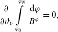 \begin{align} \frac {\partial }{\partial \vartheta _0}\int \limits _{\varphi _0}^{\varphi _N} \frac {\textrm { d} \varphi }{B^\varphi }=0, \end{align}
which is a “true” rational surface condition (Solov’ev & Shafranov, Reference Solov’ev and Shafranov1970). Using the explicit form of $H^\prime _\varphi$
in (2.34) and taking the flux “surface average” (2.10) of
$H^\prime _\varphi$
in (2.34) and taking the flux “surface average” (2.10) of $j_\parallel B$
thus eliminating the Pfirsch–Schlüter current which is driven solely by charge separation potential and, therefore, must satisfy
$j_\parallel B$
thus eliminating the Pfirsch–Schlüter current which is driven solely by charge separation potential and, therefore, must satisfy $\langle j_{\text {PS}} B\rangle = 0$
, we finally obtain the bootstrap current density
$\langle j_{\text {PS}} B\rangle = 0$
, we finally obtain the bootstrap current density $j_b$
which scales with
$j_b$
which scales with $B$
as
$B$
as
 \begin{align} \langle j_\parallel B\rangle = j_b \frac {\langle B^2\rangle }{B} = - c \lambda _{bB}\frac {\partial p}{\partial r}. \end{align}
Here, $\lambda _{bB}$
is the dimensionless geometrical factor
$\lambda _{bB}$
is the dimensionless geometrical factor $\lambda _b$
given by equation (9) of Nemov et al. (Reference Nemov, Kalyuzhnyj, Kasilov, Drevlak, Nührenberg, Kernbichler, Reiman and Monticello2004) in the case of normalization field
$\lambda _b$
given by equation (9) of Nemov et al. (Reference Nemov, Kalyuzhnyj, Kasilov, Drevlak, Nührenberg, Kernbichler, Reiman and Monticello2004) in the case of normalization field $B_0 = \langle B^2\rangle ^{1/2}$
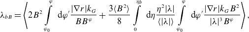 \begin{align} \lambda _{bB} = \left \langle 2 B^2 \int \limits _{\varphi _0}^\varphi \textrm { d} \varphi ^\prime \frac {|\nabla r| k_G}{B B^\varphi } + \frac {3 \langle B^2\rangle }{8} \int \limits _0^{\eta _b} \textrm { d}\eta \frac {\eta ^2 |\lambda |}{\langle |\lambda |\rangle } \int \limits _{\varphi _0}^\varphi \textrm { d} \varphi ^\prime \frac {|\nabla r|k_G B^2} {|\lambda |^3 B^\varphi } \right \rangle, \end{align}
with $\langle \ldots \rangle$
given for a closed field line by (2.10) with finite
$\langle \ldots \rangle$
given for a closed field line by (2.10) with finite $\varphi _N$
. It is convenient to express it via the mono-energetic bootstrap coefficient (2.11)
$\varphi _N$
. It is convenient to express it via the mono-energetic bootstrap coefficient (2.11)
 \begin{align} \lambda _{bB} = \frac {3 \bar D_{31}}{v \rho _L B}, \end{align}
in order to use it also for finite collisionality.
The separate contribution of trapped particle region to $\lambda _{bB}$
is obtained by replacement of the lower integration limit in (2.38) from 0 to
$\lambda _{bB}$
is obtained by replacement of the lower integration limit in (2.38) from 0 to $\eta _b+o$
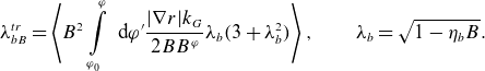 \begin{align} \lambda _{bB}^{tr} = \left \langle B^2 \int \limits _{\varphi _0}^\varphi \textrm { d} \varphi ^\prime \frac {|\nabla r| k_G}{2 B B^\varphi } \lambda _b (3+\lambda _b^2) \right \rangle, \qquad \lambda _b = \sqrt {1-\eta _b B}. \end{align}
In the usual case of small magnetic field modulation amplitude $\varepsilon _M \ll 1$
, this contribution is of the order
$\varepsilon _M \ll 1$
, this contribution is of the order $\varepsilon _{M}^{1/2}$
as compared with the first term in (2.43) and is of the order
$\varepsilon _{M}^{1/2}$
as compared with the first term in (2.43) and is of the order $\varepsilon _{M}$
as compared with the second term. Therefore, it can be ignored (Boozer & Gardner Reference Boozer and Gardner1990) as long as an exact compensation of bootstrap current,
$\varepsilon _{M}$
as compared with the second term. Therefore, it can be ignored (Boozer & Gardner Reference Boozer and Gardner1990) as long as an exact compensation of bootstrap current, $\lambda _{bB}=0$
, is not looked for.
$\lambda _{bB}=0$
, is not looked for.
The factor (2.43) matches the result of Shaing and Callen, which is a natural consequence of using the same method. Namely, $\lambda _{bB} = (1-f_c) \langle \tilde G_b \rangle / S$
where
$\lambda _{bB} = (1-f_c) \langle \tilde G_b \rangle / S$
where $S = \textrm { d} V / \textrm { d} r$
is the flux surface area, fraction of circulating particles
$S = \textrm { d} V / \textrm { d} r$
is the flux surface area, fraction of circulating particles $f_c$
is given by equation (56) of Shaing & Callen (Reference Shaing and Callen1983), and geometrical factor
$f_c$
is given by equation (56) of Shaing & Callen (Reference Shaing and Callen1983), and geometrical factor $\tilde G_b$
is given there by equations (75b) and (60c). In the case of negligible toroidal equilibrium current,
$\tilde G_b$
is given there by equations (75b) and (60c). In the case of negligible toroidal equilibrium current, $B_\vartheta =0$
, the result of Boozer & Gardner (Reference Boozer and Gardner1990) is also approximately recovered,
$B_\vartheta =0$
, the result of Boozer & Gardner (Reference Boozer and Gardner1990) is also approximately recovered, $\lambda _{bB} = \Delta _0 B_\varphi \textrm { d} r / \textrm { d} \psi + O(\varepsilon _{\text {M}})$
, where the quantity
$\lambda _{bB} = \Delta _0 B_\varphi \textrm { d} r / \textrm { d} \psi + O(\varepsilon _{\text {M}})$
, where the quantity $\Delta _0$
is given by equations (51), (53) and (54) of Boozer & Gardner (Reference Boozer and Gardner1990), ignoring the small trapped particle contribution and other corrections linear in
$\Delta _0$
is given by equations (51), (53) and (54) of Boozer & Gardner (Reference Boozer and Gardner1990), ignoring the small trapped particle contribution and other corrections linear in $\varepsilon _{M}$
(in the case of a circular tokamak,
$\varepsilon _{M}$
(in the case of a circular tokamak, $\lambda _{bB} \approx A\Delta _0$
where
$\lambda _{bB} \approx A\Delta _0$
where $A$
is the aspect ratio).
$A$
is the aspect ratio).
Note that the trapped particle distribution function here is formally the same as the one given in the implicit form by equation (54) of Shaing & Callen (Reference Shaing and Callen1983) omitting there the ripple plateau contribution absent in our case where we ignored banana precession (cross-field drift within flux surfaces) already in the starting equation (2.3). On the other hand, we obtained also the explicit expression for its odd part, (2.35), which is demonstrative for the distribution of the parallel equilibrium current in the velocity space. It can be seen that a significant part of this current (essentially of the Pfirsch–Schlüter current) flows in the boundary layers between trapped particle classes (but not in the main, trapped–passing boundary layer). The origin of these localized currents is the same as the origin of the Pfirsch–Schlüter current in all devices, i.e. they remove charge separation introduced by the radial particle drift. However, in contrast to tokamaks (and tokamak-like part of the current in stellarators) where compensation currents are produced in a long mean free path regime within a single turn of particle bounce motion due to the finite radial displacement during this time, localized currents serve to compensate charge separation by finite bounce-averaged drift, which accumulates on much longer collisional detrapping time. Interpreting the source term $s_{(1)}$
, (2.4), in the regions where it is positive as a source of ‘particles’ and where it is negative as a source of ‘anti-particles’ whose total amount generated at the flux surface is the same as the amount of ‘particles’, being a consequence of quasi-Liouville’s theorem (2.15), we see that particles (or anti-particles) accumulated in the local ripple wells due to the finite bounce-averaged drift,
$s_{(1)}$
, (2.4), in the regions where it is positive as a source of ‘particles’ and where it is negative as a source of ‘anti-particles’ whose total amount generated at the flux surface is the same as the amount of ‘particles’, being a consequence of quasi-Liouville’s theorem (2.15), we see that particles (or anti-particles) accumulated in the local ripple wells due to the finite bounce-averaged drift, $H_j \ne 0$
, can only leave the wells due to collisional scattering flux through the class boundaries (see figure 1). Since local collisional flux density generally needs not be continuous at this boundary,
$H_j \ne 0$
, can only leave the wells due to collisional scattering flux through the class boundaries (see figure 1). Since local collisional flux density generally needs not be continuous at this boundary, $\partial g_{-1}(\eta -o) /\partial \eta \ne \partial g_{-1}(\eta +o) /\partial \eta$
, a significant amount of particles (anti-particles) is re-distributed through the boundary layers, which is manifested by the
$\partial g_{-1}(\eta -o) /\partial \eta \ne \partial g_{-1}(\eta +o) /\partial \eta$
, a significant amount of particles (anti-particles) is re-distributed through the boundary layers, which is manifested by the $\delta$
-like behavior of
$\delta$
-like behavior of $g_0$
, (2.35), being, up to a factor, a parallel flow density in velocity space.
$g_0$
, (2.35), being, up to a factor, a parallel flow density in velocity space.
The asymptotic series expansion (2.17) can be continued to the next order, leading to the correction $g_1$
. This correction, however, has a non-integrable singularity at class-transition boundaries,
$g_1$
. This correction, however, has a non-integrable singularity at class-transition boundaries, $g_1 \propto (\eta - \eta _c)^{-2}$
(in contrast to integrable singularity of
$g_1 \propto (\eta - \eta _c)^{-2}$
(in contrast to integrable singularity of $g_0 \propto \log |\eta - \eta _c|$
), which is a consequence of finite geodesic curvature at respective local field maxima. Therefore, contributions of different order corrections to the collisional flux density in the matching conditions (2.31) become comparable at finite collisionality for
$g_0 \propto \log |\eta - \eta _c|$
), which is a consequence of finite geodesic curvature at respective local field maxima. Therefore, contributions of different order corrections to the collisional flux density in the matching conditions (2.31) become comparable at finite collisionality for $|\eta -\eta _c| =\delta \eta \propto l_c^{-1/2} \propto \nu ^{1/2}$
, where
$|\eta -\eta _c| =\delta \eta \propto l_c^{-1/2} \propto \nu ^{1/2}$
, where $\partial g_{0}(\eta ) /\partial \eta \sim \delta \eta ^{-1}$
and
$\partial g_{0}(\eta ) /\partial \eta \sim \delta \eta ^{-1}$
and $\partial g_{1}(\eta ) /\partial \eta \sim l_c^{-1} \delta \eta ^{-3}$
. In other words, the expansion (2.17) breaks down at the edge of the boundary layer of width
$\partial g_{1}(\eta ) /\partial \eta \sim l_c^{-1} \delta \eta ^{-3}$
. In other words, the expansion (2.17) breaks down at the edge of the boundary layer of width $\delta \eta$
. Respectively, matching interval
$\delta \eta$
. Respectively, matching interval $o$
in (2.28), which is an infinitesimal for vanishing collisionality, should satisfy
$o$
in (2.28), which is an infinitesimal for vanishing collisionality, should satisfy $\delta \eta \ll o \ll \eta$
for finite collisionality, which means that the error of the asymptotic solution scales with
$\delta \eta \ll o \ll \eta$
for finite collisionality, which means that the error of the asymptotic solution scales with $\sqrt {\nu }$
rather than with
$\sqrt {\nu }$
rather than with $\nu$
. Since the particle–anti-particle re-distribution flux manifested by
$\nu$
. Since the particle–anti-particle re-distribution flux manifested by $\delta$
-functions in asymptotic expression (2.35) for
$\delta$
-functions in asymptotic expression (2.35) for $g_0$
is independent of collisionality, we can estimate the odd part of the distribution function which carries this flux in the class-transition boundary layers as
$g_0$
is independent of collisionality, we can estimate the odd part of the distribution function which carries this flux in the class-transition boundary layers as $g^{\text{odd}} \propto \delta \eta ^{-1} \propto l_c^{1/2} \propto \nu ^{-1/2}$
.
$g^{\text{odd}} \propto \delta \eta ^{-1} \propto l_c^{1/2} \propto \nu ^{-1/2}$
.
As shown below, the presence of these strong parallel flows in class-transition boundary layers is actually responsible for the ‘anomalous’ behavior of the bootstrap current at finite collisionality.
2.2.2. Adjoint problem
The asymptotic solution of the adjoint problem has been derived by Helander et al. (Reference Helander, Geiger and Maassberg2011) omitting in the correction $g_0$
, which determines particle flux, the
$g_0$
, which determines particle flux, the $\varphi$
independent part
$\varphi$
independent part $\bar g_0$
which does not contribute to this flux and, respectively, is not needed for the Ware-pinch coefficient. Here, we extend this derivation in order to obtain the complete even part of this correction useful for the interpretation of numerical examples in the following sections. The leading-order asymptotic solution is odd in
$\bar g_0$
which does not contribute to this flux and, respectively, is not needed for the Ware-pinch coefficient. Here, we extend this derivation in order to obtain the complete even part of this correction useful for the interpretation of numerical examples in the following sections. The leading-order asymptotic solution is odd in $\sigma$
and is given by the bounce-averaged equation (2.20) for the source
$\sigma$
and is given by the bounce-averaged equation (2.20) for the source $s_{(3)}$
, see (2.4), with the same boundary conditions as previously as
$s_{(3)}$
, see (2.4), with the same boundary conditions as previously as
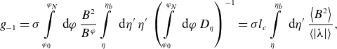 \begin{align} g_{-1} = \sigma \int \limits _{\varphi _0}^{\varphi _N}\textrm { d} \varphi \;\frac {B^2}{B^\varphi } \int \limits ^{\eta _b}_\eta \textrm { d} \eta ^\prime \;\eta ^\prime \; \left (\int \limits _{\varphi _0}^{\varphi _N}\textrm { d} \varphi \;D_\eta \right )^{-1} =\sigma l_c \int \limits ^{\eta _b}_\eta \textrm { d} \eta ^\prime \; \frac {\left \langle B^2\right \rangle } {\left \langle |\lambda |\right \rangle }, \end{align}
in the passing region, and $g_{-1}=0$
in the trapped region. The next-order correction results from (2.19) in the trapped region in
$g_{-1}=0$
in the trapped region. The next-order correction results from (2.19) in the trapped region in
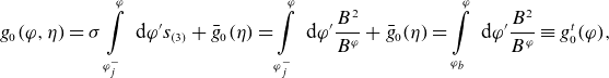 \begin{align} g_0(\varphi, \eta )=\sigma \int \limits _{\varphi _j^-}^\varphi \textrm { d} \varphi ^\prime s_{(3)}+\bar g_0(\eta ) =\int \limits _{\varphi _j^-}^\varphi \textrm { d} \varphi ^\prime \frac {B^2}{B^\varphi }+\bar g_0(\eta ) =\int \limits _{\varphi _b}^\varphi \textrm { d} \varphi ^\prime \frac {B^2}{B^\varphi }\equiv g_0^t(\varphi ), \end{align}
where we integrated (2.23)
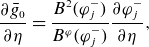 \begin{align} \frac {\partial \bar g_0}{\partial \eta }=\frac {B^2(\varphi _j^-)}{B^\varphi (\varphi _j^-)}\frac {\partial \varphi _j^-}{\partial \eta }, \end{align}
from the trapped–passing boundary and included an arbitrary integration constant into the lower integration limit $\varphi _b$
being, therefore, an arbitrary constant too. This constant is the same for all classes due to continuity of
$\varphi _b$
being, therefore, an arbitrary constant too. This constant is the same for all classes due to continuity of $g_0$
at class-transition boundaries.
$g_0$
at class-transition boundaries.
In the passing region, solutions of (2.19) and (2.23) result in
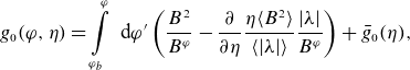 \begin{align} g_0(\varphi, \eta ) = \int \limits _{\varphi _b}^\varphi \textrm { d} \varphi ^\prime \left ( \frac {B^2}{B^\varphi } - \frac {\partial }{\partial \eta } \frac {\eta \langle B^2 \rangle }{\langle |\lambda |\rangle } \frac {|\lambda |}{B^\varphi } \right ) + \bar g_0(\eta ), \end{align}
where
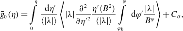 \begin{align} \bar g_0(\eta ) = \int \limits _0^\eta \frac {\textrm { d} \eta ^\prime }{\langle |\lambda |\rangle } \left \langle |\lambda | \frac {\partial ^2}{\partial {\eta ^\prime }^2} \frac {\eta ^\prime \langle B^2 \rangle }{\langle |\lambda |\rangle } \int \limits _{\varphi _b}^\varphi \textrm { d} \varphi ^\prime \frac {|\lambda |}{B^\varphi } \right \rangle +C_\sigma, \end{align}
and where $C_\sigma$
are different integration constants of (2.23) for
$C_\sigma$
are different integration constants of (2.23) for $\sigma =\pm 1$
. Similar to the solution of the direct problem, derivative
$\sigma =\pm 1$
. Similar to the solution of the direct problem, derivative $\partial g_0/\partial \eta$
of the function (2.49) does not depend on
$\partial g_0/\partial \eta$
of the function (2.49) does not depend on $\varphi _b$
in the passing region. Actually, the lower integration limit
$\varphi _b$
in the passing region. Actually, the lower integration limit $\varphi _b$
in (2.49) and (2.50) enters
$\varphi _b$
in (2.49) and (2.50) enters $g_0$
via a periodic function of
$g_0$
via a periodic function of $\varphi _b$
which adds up to the integration constant
$\varphi _b$
which adds up to the integration constant $C_\sigma$
(this follows from explicit evaluation of
$C_\sigma$
(this follows from explicit evaluation of $\partial g_0 /\partial \varphi _b = \left (\langle B^2 \rangle - B^2(\varphi _b)\right ) /B^\varphi (\varphi _b)$
whose integral over the whole range
$\partial g_0 /\partial \varphi _b = \left (\langle B^2 \rangle - B^2(\varphi _b)\right ) /B^\varphi (\varphi _b)$
whose integral over the whole range $\varphi _0\lt \varphi _b\lt \varphi _N$
is zero). Function
$\varphi _0\lt \varphi _b\lt \varphi _N$
is zero). Function $g_0$
has an integrable logarithmic singularity at the trapped–passing boundary,
$g_0$
has an integrable logarithmic singularity at the trapped–passing boundary, $g_0 \propto \log (\eta _b-\eta )$
, in particular, due to such singularity of
$g_0 \propto \log (\eta _b-\eta )$
, in particular, due to such singularity of $\partial \langle |\lambda |\rangle / \partial \eta$
which, up to a constant factor, is a bounce time. Next-order correction shows again that series expansion breaks down in the boundary layer,
$\partial \langle |\lambda |\rangle / \partial \eta$
which, up to a constant factor, is a bounce time. Next-order correction shows again that series expansion breaks down in the boundary layer, $|\eta _b-\eta | \leqslant \delta \eta \propto l_c^{-1/2}$
.
$|\eta _b-\eta | \leqslant \delta \eta \propto l_c^{-1/2}$
.
In order to fully determine $g_0$
in the whole phase space we must express three integration constants,
$g_0$
in the whole phase space we must express three integration constants, $\varphi _b$
and
$\varphi _b$
and $C_\sigma$
, via a single constant which is the only degree of freedom re-defining an equilibrium Maxwellian. For that, we must match the solutions through the trapped–passing boundary where
$C_\sigma$
, via a single constant which is the only degree of freedom re-defining an equilibrium Maxwellian. For that, we must match the solutions through the trapped–passing boundary where $g_0$
is singular, but first it is convenient to split
$g_0$
is singular, but first it is convenient to split $g_0$
into even and odd parts in
$g_0$
into even and odd parts in $\sigma$
,
$\sigma$
, $g_0=g_0^{\text{even}}+g_0^{\text{odd}}$
, where
$g_0=g_0^{\text{even}}+g_0^{\text{odd}}$
, where $g_0^{\text{even}}$
is given by (2.47)–(2.50) with replacement of
$g_0^{\text{even}}$
is given by (2.47)–(2.50) with replacement of $C_\sigma$
by a constant
$C_\sigma$
by a constant $C_{\text{even}}$
and
$C_{\text{even}}$
and $g_0^{\text{odd}}=\sigma C_{\text{odd}}\Theta (\eta _b-\eta )$
, where
$g_0^{\text{odd}}=\sigma C_{\text{odd}}\Theta (\eta _b-\eta )$
, where $\Theta (x)$
is a Heaviside step function, and
$\Theta (x)$
is a Heaviside step function, and $C_{\text{odd}}$
is another constant.
$C_{\text{odd}}$
is another constant.
Function $g_0^{\text{odd}}$
is of no interest in the following since it does not contribute to the Ware pinch but only provides a correction to the leading-order solution (2.46). As for
$g_0^{\text{odd}}$
is of no interest in the following since it does not contribute to the Ware pinch but only provides a correction to the leading-order solution (2.46). As for $g_0^{\text{even}}$
, we still need to determine it formally in the boundary layer identifying there its most singular part. For this purpose, we take the odd part of (2.3) and, similar to (2.32), and integrate it across the boundary layer ignoring the contribution of the source term and retaining only the leading-order solution (2.46) in the collisional flux through the boundaries of integration domain
$g_0^{\text{even}}$
, we still need to determine it formally in the boundary layer identifying there its most singular part. For this purpose, we take the odd part of (2.3) and, similar to (2.32), and integrate it across the boundary layer ignoring the contribution of the source term and retaining only the leading-order solution (2.46) in the collisional flux through the boundaries of integration domain
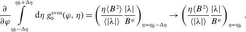 \begin{align} \frac {\partial }{\partial \varphi } \int \limits _{\eta _b-\Delta \eta }^{\eta _b+\Delta \eta }\textrm { d} \eta \; g_0^{\text{even}}(\varphi, \eta ) = \left (\frac {\eta \langle B^2 \rangle }{\langle |\lambda |\rangle } \frac {|\lambda |}{B^\varphi }\right )_{\eta =\eta _b-\Delta \eta } \rightarrow \left (\frac {\eta \langle B^2 \rangle }{\langle |\lambda |\rangle } \frac {|\lambda |}{B^\varphi }\right )_{\eta =\eta _b}. \end{align}
Here, $\delta \eta \ll \Delta \eta \ll \eta _b$
,
$\delta \eta \ll \Delta \eta \ll \eta _b$
, $\delta \eta$
is the boundary layer width and the last expression corresponds to the collisionless limit
$\delta \eta$
is the boundary layer width and the last expression corresponds to the collisionless limit $\Delta \eta \rightarrow 0$
. Thus
$\Delta \eta \rightarrow 0$
. Thus $g_0^{\text{even}}$
can be formally presented near the trapped passing boundary as
$g_0^{\text{even}}$
can be formally presented near the trapped passing boundary as
 \begin{align} g_0^{\text{even}}=\delta (\eta _b-\eta )\left (\int \limits _{\varphi _b}^\varphi \textrm { d} \varphi ^\prime \frac {\eta \langle B^2 \rangle }{\langle |\lambda |\rangle } \frac {|\lambda |}{B^\varphi }+C_{\text{bou}} \right )+o(\delta \eta ^{-1}), \end{align}
where $C_{\text{bou}}$
is yet another integration constant, and the last term provides a vanishing contribution to the
$C_{\text{bou}}$
is yet another integration constant, and the last term provides a vanishing contribution to the $\eta$
-integral in (2.51). Similar to the passing particle solution (2.49), which is defined for the whole closed field line and which is a periodic function of
$\eta$
-integral in (2.51). Similar to the passing particle solution (2.49), which is defined for the whole closed field line and which is a periodic function of $\varphi$
with period
$\varphi$
with period $\varphi _N-\varphi _0$
, boundary layer solution (2.52) is formally defined for the whole field period too and must be a periodic function as well. In order to be periodic, function (2.52) must be discontinuous over the variable
$\varphi _N-\varphi _0$
, boundary layer solution (2.52) is formally defined for the whole field period too and must be a periodic function as well. In order to be periodic, function (2.52) must be discontinuous over the variable $\varphi$
, and the only point where a jump restoring the periodicity is possible, as we see below, is the global maximum point
$\varphi$
, and the only point where a jump restoring the periodicity is possible, as we see below, is the global maximum point $\varphi =\varphi _0$
(and
$\varphi =\varphi _0$
(and $\varphi =\varphi _N$
). This discontinuity requirement leads to a certain paradox because, according to (2.3), the distribution function is continuous with
$\varphi =\varphi _N$
). This discontinuity requirement leads to a certain paradox because, according to (2.3), the distribution function is continuous with $\varphi$
everywhere in the range where
$\varphi$
everywhere in the range where $\eta B(\varphi )\lt 1$
, which includes the whole trapped–passing boundary approached from the passing side,
$\eta B(\varphi )\lt 1$
, which includes the whole trapped–passing boundary approached from the passing side, $\eta =\eta _b-0$
, which in turn seems to contradict the discontinuity of the function (2.52). To resolve this paradox, we note that a formal representation with a
$\eta =\eta _b-0$
, which in turn seems to contradict the discontinuity of the function (2.52). To resolve this paradox, we note that a formal representation with a $\delta$
-function actually assumes a small but finite width of the boundary layer, which is partly located in the passing particle region where the distribution is strictly continuous with
$\delta$
-function actually assumes a small but finite width of the boundary layer, which is partly located in the passing particle region where the distribution is strictly continuous with $\varphi$
, and partly in the trapped particle region where it is continuous too except a small forbidden region with
$\varphi$
, and partly in the trapped particle region where it is continuous too except a small forbidden region with $\eta B(\varphi )\gt 1$
located near the global maximum. Discontinuity of
$\eta B(\varphi )\gt 1$
located near the global maximum. Discontinuity of $g_0^{\text{even}}$
within this trapped part of the boundary layer is sufficient to provide the required jumps restoring the periodicity.
$g_0^{\text{even}}$
within this trapped part of the boundary layer is sufficient to provide the required jumps restoring the periodicity.
Similarly to the boundary layer, the periodicity argument means for the trapped particle distribution that its integral form (2.47) determined via $\varphi _b$
from the interval
$\varphi _b$
from the interval $\varphi _0\lt \varphi _b\lt \varphi _N$
can be used only in the same interval,
$\varphi _0\lt \varphi _b\lt \varphi _N$
can be used only in the same interval, $\varphi _0\lt \varphi \lt \varphi _N$
. Thus, an extension of (2.47) and (2.51) to the infinite
$\varphi _0\lt \varphi \lt \varphi _N$
. Thus, an extension of (2.47) and (2.51) to the infinite $\varphi$
range is obtained replacing there the lower integration limit
$\varphi$
range is obtained replacing there the lower integration limit $\varphi _b$
with
$\varphi _b$
with $\varphi _b + (\varphi _N-\varphi _0) \left [(\varphi -\varphi _0)/(\varphi _N-\varphi _0)\right ]$
, where
$\varphi _b + (\varphi _N-\varphi _0) \left [(\varphi -\varphi _0)/(\varphi _N-\varphi _0)\right ]$
, where $[\ldots ]$
denotes the integer part. As already mentioned above, the passing particle solution (2.49) is valid for the infinite
$[\ldots ]$
denotes the integer part. As already mentioned above, the passing particle solution (2.49) is valid for the infinite $\varphi$
range as is. We can actually combine all these periodic solutions for
$\varphi$
range as is. We can actually combine all these periodic solutions for $g_0^{\text{even}}$
in one multiplying so extended trapped particle solution (2.47) with
$g_0^{\text{even}}$
in one multiplying so extended trapped particle solution (2.47) with $\Theta (\eta -\eta _b)$
, adding an even part of the passing particle solution (2.49) multiplied with
$\Theta (\eta -\eta _b)$
, adding an even part of the passing particle solution (2.49) multiplied with $\Theta (\eta _b-\eta )$
and then adding an extended boundary layer solution (2.52).
$\Theta (\eta _b-\eta )$
and then adding an extended boundary layer solution (2.52).
In order to eliminate from such a combined solution, all but one unknown constants out of three, $\varphi _b$
,
$\varphi _b$
, $C_{\text{even}}$
and
$C_{\text{even}}$
and $C_{\text{bou}}$
, we use the stellarator symmetry of our closed field line such that
$C_{\text{bou}}$
, we use the stellarator symmetry of our closed field line such that $B(2\varphi _s-\varphi )=B(\varphi )$
and
$B(2\varphi _s-\varphi )=B(\varphi )$
and $B^\varphi (2\varphi _s-\varphi )=B^\varphi (\varphi )$
, where
$B^\varphi (2\varphi _s-\varphi )=B^\varphi (\varphi )$
, where $\varphi _s$
is a symmetry point. We use the fact that the stellarator-symmetric part of the generalized Spitzer function
$\varphi _s$
is a symmetry point. We use the fact that the stellarator-symmetric part of the generalized Spitzer function $g=g_{(3)}$
given by
$g=g_{(3)}$
given by $g_{\text{sym}}(\varphi, \eta, \sigma )\equiv \left (g(\varphi, \eta, \sigma )+g^\ast (\varphi, \eta, \sigma )\right )/2$
with
$g_{\text{sym}}(\varphi, \eta, \sigma )\equiv \left (g(\varphi, \eta, \sigma )+g^\ast (\varphi, \eta, \sigma )\right )/2$
with $g^\ast (\varphi, \eta, \sigma ) \equiv g(2\varphi _s-\varphi, \eta, -\sigma )$
can only be a constant. Namely, it can be checked that
$g^\ast (\varphi, \eta, \sigma ) \equiv g(2\varphi _s-\varphi, \eta, -\sigma )$
can only be a constant. Namely, it can be checked that $g^\ast$
satisfies the same (2.3) but with an opposite sign of the source
$g^\ast$
satisfies the same (2.3) but with an opposite sign of the source $s_{(3)}$
and, therefore,
$s_{(3)}$
and, therefore, $g^\ast =-g + C$
, where
$g^\ast =-g + C$
, where $C$
is an arbitrary constant. Thus,
$C$
is an arbitrary constant. Thus, $g_{\text{sym}}=C/2$
in the whole phase space. Introducing now a stellarator-antisymmetric part of the distribution function,
$g_{\text{sym}}=C/2$
in the whole phase space. Introducing now a stellarator-antisymmetric part of the distribution function, $g_{\text{asym}}(\varphi, \eta, \sigma )\equiv \left (g(\varphi, \eta, \sigma )-g^\ast (\varphi, \eta, \sigma )\right )/2$
, we can split our solution
$g_{\text{asym}}(\varphi, \eta, \sigma )\equiv \left (g(\varphi, \eta, \sigma )-g^\ast (\varphi, \eta, \sigma )\right )/2$
, we can split our solution $g_0^{\text{even}}$
into stellarator-symmetric and stellarator-antisymmetric parts,
$g_0^{\text{even}}$
into stellarator-symmetric and stellarator-antisymmetric parts, $g_0^{\text{even}} = g_{\text{sym}}^{\text{even}}+g_{\text{asym}}^{\text{even}}$
. Thus, we obtain that stellarator-antisymmetric part of the combined
$g_0^{\text{even}} = g_{\text{sym}}^{\text{even}}+g_{\text{asym}}^{\text{even}}$
. Thus, we obtain that stellarator-antisymmetric part of the combined $g_0^{\text{even}}$
does not contain any unknown and is determined by
$g_0^{\text{even}}$
does not contain any unknown and is determined by
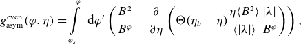 \begin{align} g_{\text{asym}}^{\text{even}}(\varphi, \eta ) = \int \limits _{\varphi _s}^\varphi \textrm { d} \varphi ^\prime \left ( \frac {B^2}{B^\varphi } - \frac {\partial }{\partial \eta } \left ( \Theta (\eta _b-\eta ) \frac {\eta \langle B^2 \rangle }{\langle |\lambda |\rangle } \frac {|\lambda |}{B^\varphi } \right ) \right ), \end{align}
where $\varphi _s$
is fixed now to a second stellarator symmetry point
$\varphi _s$
is fixed now to a second stellarator symmetry point $\varphi _s=(\varphi _0+\varphi _N)/2$
which necessarily exists besides the global maximum point
$\varphi _s=(\varphi _0+\varphi _N)/2$
which necessarily exists besides the global maximum point $\varphi _0$
. Solution (2.53) is given here only for
$\varphi _0$
. Solution (2.53) is given here only for $\varphi _0\lt \varphi \lt \varphi _N$
and can be extended to the infinite
$\varphi _0\lt \varphi \lt \varphi _N$
and can be extended to the infinite $\varphi$
range replacing there
$\varphi$
range replacing there $\varphi _s$
with
$\varphi _s$
with $\varphi _s + (\varphi _N-\varphi _0) \left [(\varphi -\varphi _0)/(\varphi _N-\varphi _0)\right ]$
. Such an extended expression is stellarator antisymmetric with respect to symmetry points of both kinds (in particular, anti-symmetry with respect to field maximum points
$\varphi _s + (\varphi _N-\varphi _0) \left [(\varphi -\varphi _0)/(\varphi _N-\varphi _0)\right ]$
. Such an extended expression is stellarator antisymmetric with respect to symmetry points of both kinds (in particular, anti-symmetry with respect to field maximum points $\varphi _0 + k(\varphi _N-\varphi _0)$
, where
$\varphi _0 + k(\varphi _N-\varphi _0)$
, where $k$
are integers is enabled by the discontinuity of the extended lower integration limit at those points) and is independent of an arbitrary constant
$k$
are integers is enabled by the discontinuity of the extended lower integration limit at those points) and is independent of an arbitrary constant $\varphi _b$
.
$\varphi _b$
.
In turn, all the unknown constants enter the stellarator-symmetric part of the combined solution $g_0^{\text{even}}$
which is of the form
$g_0^{\text{even}}$
which is of the form
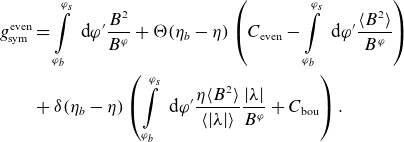 \begin{eqnarray} g_{\text{sym}}^{\text{even}}\;&=&\; \int \limits _{\varphi _b}^{\varphi _s}\textrm { d} \varphi ^\prime \frac {B^2}{B^\varphi } + \Theta (\eta _b-\eta ) \left (C_{\text{even}} -\int \limits _{\varphi _b}^{\varphi _s}\textrm { d} \varphi ^\prime \frac {\langle B^2\rangle }{B^\varphi }\right ) \nonumber \\ &+&\; \delta (\eta _b-\eta )\left (\int \limits _{\varphi _b}^{\varphi _s}\textrm { d} \varphi ^\prime \frac {\eta \langle B^2 \rangle }{\langle |\lambda |\rangle } \frac {|\lambda |}{B^\varphi }+C_{\text{bou}} \right ). \end{eqnarray}
Since this function can only be a constant, we must set $C_{\text{even}}$
and
$C_{\text{even}}$
and $C_{\text{bou}}$
so that they annihilate respective brackets multiplying the Heaviside function and
$C_{\text{bou}}$
so that they annihilate respective brackets multiplying the Heaviside function and $\delta$
-function which permits setting
$\delta$
-function which permits setting $\eta =\eta _b$
in the sub-integrand in the latter bracket. Finally, the remaining first term can be, as usual, absorbed into the equilibrium Maxwellian so that the whole final solution
$\eta =\eta _b$
in the sub-integrand in the latter bracket. Finally, the remaining first term can be, as usual, absorbed into the equilibrium Maxwellian so that the whole final solution $g_0^{\text{even}}=g_{\text{asym}}^{\text{even}}$
is given by (2.53). The only difference of this solution from equation (12) of Helander et al. (Reference Helander, Geiger and Maassberg2011) is the lower integration limit
$g_0^{\text{even}}=g_{\text{asym}}^{\text{even}}$
is given by (2.53). The only difference of this solution from equation (12) of Helander et al. (Reference Helander, Geiger and Maassberg2011) is the lower integration limit $\varphi _s$
which is the second symmetry point (usually global minimum) instead of a global maximum point
$\varphi _s$
which is the second symmetry point (usually global minimum) instead of a global maximum point $\varphi _0$
.
$\varphi _0$
.
Substituting (2.46) and (2.53) for $g_{(3)}=g_{-1}+g_0$
in (2.11) we obtain the mono-energetic Ware-pinch coefficient as
$g_{(3)}=g_{-1}+g_0$
in (2.11) we obtain the mono-energetic Ware-pinch coefficient as
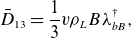 \begin{align} \bar D_{13} = \frac {1}{3} v \rho _L B \lambda _{bB}^\dagger, \end{align}
with the geometrical factor given by
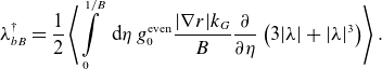 \begin{align} \lambda _{bB}^\dagger =\frac {1}{2} \left \langle \int \limits _0^{1/B} \textrm { d}\eta \; g_0^{\text{even}} \frac {|\nabla r|k_G} {B} \frac {\partial }{\partial \eta }\left (3|\lambda |+|\lambda |^3\right ) \right \rangle . \end{align}
Exchanging in this expression the integration order over $\eta$
and
$\eta$
and $\varphi$
and integrating by parts over
$\varphi$
and integrating by parts over $\varphi$
within the motion domains
$\varphi$
within the motion domains $\varphi _{\textrm{beg}}(\eta ) \lt \varphi \lt \varphi _{\textrm{end}}(\eta )$
we use conditions (2.15) to eliminate contribution from the integration limits. Thus, only the derivative
$\varphi _{\textrm{beg}}(\eta ) \lt \varphi \lt \varphi _{\textrm{end}}(\eta )$
we use conditions (2.15) to eliminate contribution from the integration limits. Thus, only the derivative $\partial g_0 / \partial \varphi$
can contribute. Integrating the result by parts over
$\partial g_0 / \partial \varphi$
can contribute. Integrating the result by parts over $\eta$
in the term with
$\eta$
in the term with $\Theta (\eta _b-\eta )$
, one finally obtains
$\Theta (\eta _b-\eta )$
, one finally obtains $\lambda _{bB}^\dagger =\lambda _{bB}$
given by (2.43).
$\lambda _{bB}^\dagger =\lambda _{bB}$
given by (2.43).
It should be noted that, in contrast to the solution of the direct problem, the solution of the adjoint problem (2.53) is regular at all class-transition boundaries and has a $\delta$
-like behavior only in the boundary layer at the trapped–passing boundary where finite collisionality scaling of
$\delta$
-like behavior only in the boundary layer at the trapped–passing boundary where finite collisionality scaling of $g^{\text{even}}$
is
$g^{\text{even}}$
is $g^{\text{even}}\sim l_c^{1/2} \sim \nu ^{-1/2}$
. As shown below, interaction of this boundary layer with locally trapped particle domains is responsible for the ‘anomalous’ behavior of the Ware-pinch coefficient at finite collisionalities.
$g^{\text{even}}\sim l_c^{1/2} \sim \nu ^{-1/2}$
. As shown below, interaction of this boundary layer with locally trapped particle domains is responsible for the ‘anomalous’ behavior of the Ware-pinch coefficient at finite collisionalities.
2.3. Finite collisionality, numerical examples
For the numerical tests, we use the drift kinetic equation solver NEO-2 (Kernbichler et al. Reference Kernbichler, Kasilov, Leitold, Nemov and Allmaier2008; Kasilov et al. Reference Kasilov, Kernbichler, Martitsch, Maassberg and Heyn2014; Martitsch et al. Reference Martitsch2016; Kernbichler et al. Reference Kernbichler, Kasilov, Kapper, Martitsch, Nemov and Heyn2016; Kapper et al. Reference Kapper, Kasilov, Kernbichler, Martitsch, Heyn, Marushchenko and Turkin2016, Reference Kapper, Kasilov, Kernbichler and Aradi2018), which, generally, employs a full linearized collision operator including the relativistic effects (Kapper et al. Reference Kapper, Kasilov, Kernbichler and Aradi2018). Here, we restrict its collision operator to the Lorentz model only. The magnetic field model corresponds to a circular tokamak with concentric flux surfaces ( $\beta =0$
) and with a toroidal ripple-like perturbation, given in Boozer coordinates by
$\beta =0$
) and with a toroidal ripple-like perturbation, given in Boozer coordinates by
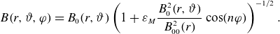 \begin{align} B(r,\vartheta, \varphi ) = B_0(r,\vartheta ) \left (1+\varepsilon _M \frac {B_0^2(r,\vartheta )}{B_{00}^2(r)}\cos (n\varphi )\right )^{-1/2}. \end{align}
Here, $B_0(r,\vartheta )$
is the unperturbed field,
$B_0(r,\vartheta )$
is the unperturbed field, $B_{00}(r)$
is the
$B_{00}(r)$
is the $(m,n)=(0,0)$
harmonic of this field and
$(m,n)=(0,0)$
harmonic of this field and $\varepsilon _M$
is the modulation amplitude. It can be checked that this field fulfills “true surface” condition (2.41) at all rational flux surfaces, which is a property useful for the studies of bootstrap resonances briefly discussed in § 4.1. We fix
$\varepsilon _M$
is the modulation amplitude. It can be checked that this field fulfills “true surface” condition (2.41) at all rational flux surfaces, which is a property useful for the studies of bootstrap resonances briefly discussed in § 4.1. We fix $n=3$
and
$n=3$
and $\varepsilon _M=0.1$
and consider two cases of the rotational transform
$\varepsilon _M=0.1$
and consider two cases of the rotational transform $\iota =1/q$
with
$\iota =1/q$
with $\iota =1/4$
and
$\iota =1/4$
and $\iota =2/5$
, where the field line is closed after one and two poloidal turns, respectively.
$\iota =2/5$
, where the field line is closed after one and two poloidal turns, respectively.
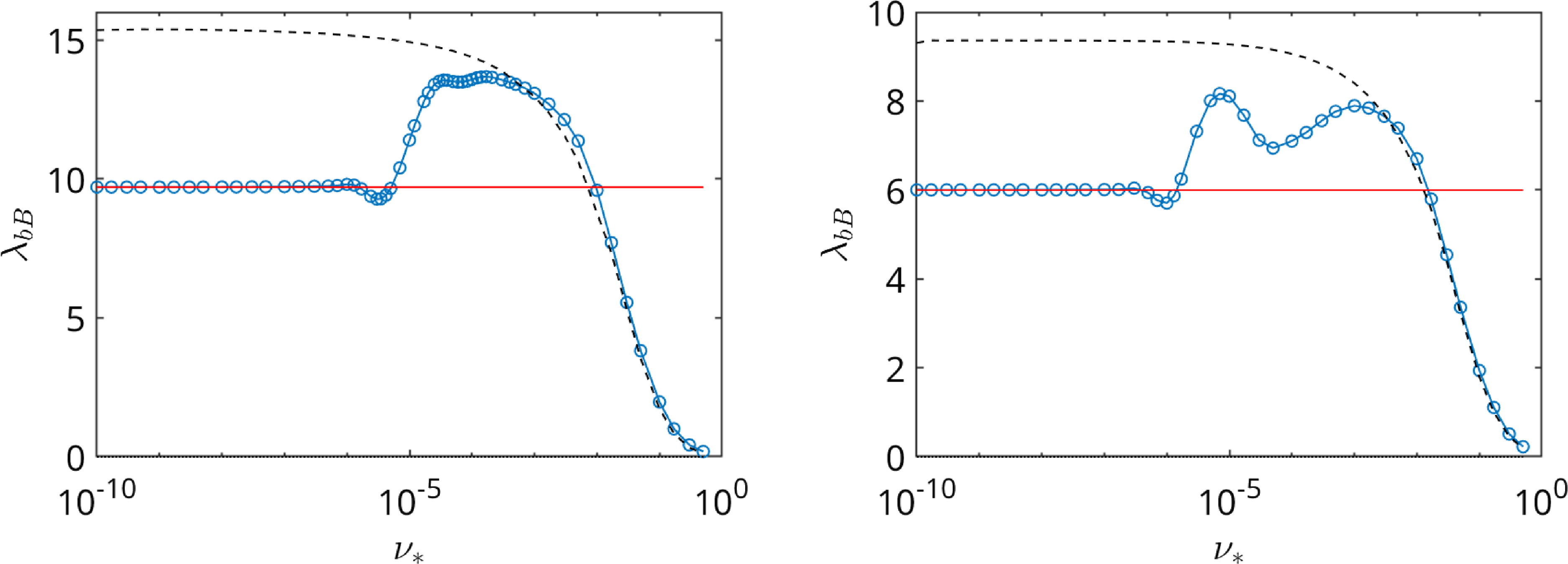
Figure 2. Geometrical factor $\lambda _{bB}$
computed by NEO-2 (blue) for different normalized collisionalities
$\lambda _{bB}$
computed by NEO-2 (blue) for different normalized collisionalities $\nu _\ast$
and computed from the Shaing–Callen limit (2.43) evaluated by NEO (red) for
$\nu _\ast$
and computed from the Shaing–Callen limit (2.43) evaluated by NEO (red) for $\iota =1/4$
(left) and
$\iota =1/4$
(left) and $\iota =2/5$
(right). Black dashed lines show the result of NEO-2 for axisymmetric fields (
$\iota =2/5$
(right). Black dashed lines show the result of NEO-2 for axisymmetric fields ( $\varepsilon _{M}=0$
).
$\varepsilon _{M}=0$
).
The normalized bootstrap coefficient (2.44) computed by NEO-2 for the above two cases as a function of the normalized collisionality $\nu _\ast = \pi R \nu _\perp / v = \pi R /(2 l_c) = \pi \iota \nu ^\ast$
, where
$\nu _\ast = \pi R \nu _\perp / v = \pi R /(2 l_c) = \pi \iota \nu ^\ast$
, where $R$
is the major radius of the magnetic axis and
$R$
is the major radius of the magnetic axis and $\nu ^\ast$
is the definition of Beidler et al. (Reference Beidler2011), is compared with the Shaing–Callen limit (2.43) in figure 2. (The latter asymptotic limit is computed here using the code NEO (Nemov et al. Reference Nemov, Kasilov, Kernbichler and Heyn1999, Reference Nemov, Kalyuzhnyj, Kasilov, Drevlak, Nührenberg, Kernbichler, Reiman and Monticello2004), which should not be confused with the drift kinetic code of Belli and Candy (Belli & Candy Reference Belli and Candy2015) having the same name.) It can be seen that the asymptotic value is abruptly reached in both cases at rather low collisionalities
$\nu ^\ast$
is the definition of Beidler et al. (Reference Beidler2011), is compared with the Shaing–Callen limit (2.43) in figure 2. (The latter asymptotic limit is computed here using the code NEO (Nemov et al. Reference Nemov, Kasilov, Kernbichler and Heyn1999, Reference Nemov, Kalyuzhnyj, Kasilov, Drevlak, Nührenberg, Kernbichler, Reiman and Monticello2004), which should not be confused with the drift kinetic code of Belli and Candy (Belli & Candy Reference Belli and Candy2015) having the same name.) It can be seen that the asymptotic value is abruptly reached in both cases at rather low collisionalities $\nu _\ast \sim 10^{-6}$
with the collisional
$\nu _\ast \sim 10^{-6}$
with the collisional $\lambda _{bB}$
dropping briefly below the Shaing–Callen limit prior to convergence. Naturally, the normalized Ware-pinch coefficient
$\lambda _{bB}$
dropping briefly below the Shaing–Callen limit prior to convergence. Naturally, the normalized Ware-pinch coefficient $\lambda _{bB}^\dagger$
, (2.55), differs from bootstrap coefficient only by small numerical errors and cannot be distinguished in this plot. For the studies of the off-set of collisional bootstrap (Ware-pinch) coefficient from the asymptotic value seen at low but finite collisionality, we examine the distribution function computed by NEO-2 in the direct and adjoint problems separately.
$\lambda _{bB}^\dagger$
, (2.55), differs from bootstrap coefficient only by small numerical errors and cannot be distinguished in this plot. For the studies of the off-set of collisional bootstrap (Ware-pinch) coefficient from the asymptotic value seen at low but finite collisionality, we examine the distribution function computed by NEO-2 in the direct and adjoint problems separately.
2.3.1. Direct problem
An odd part of the distribution function perturbation $g^{\text{odd}}$
responsible for the bootstrap current in the direct problem is shown in figure 3. One can observe the appearance of boundary layers around class-transition boundaries (but not at the trapped–passing boundary) with decreasing collisionality. It can be seen that, at lowest collisionality,
$g^{\text{odd}}$
responsible for the bootstrap current in the direct problem is shown in figure 3. One can observe the appearance of boundary layers around class-transition boundaries (but not at the trapped–passing boundary) with decreasing collisionality. It can be seen that, at lowest collisionality, $\nu _\ast =10^{-6}$
, where the asymptotic limit is reached in figure 2, the highest class-transition boundary layer corresponding to two highest local maxima becomes clearly separated from the trapped–passing boundary.
$\nu _\ast =10^{-6}$
, where the asymptotic limit is reached in figure 2, the highest class-transition boundary layer corresponding to two highest local maxima becomes clearly separated from the trapped–passing boundary.
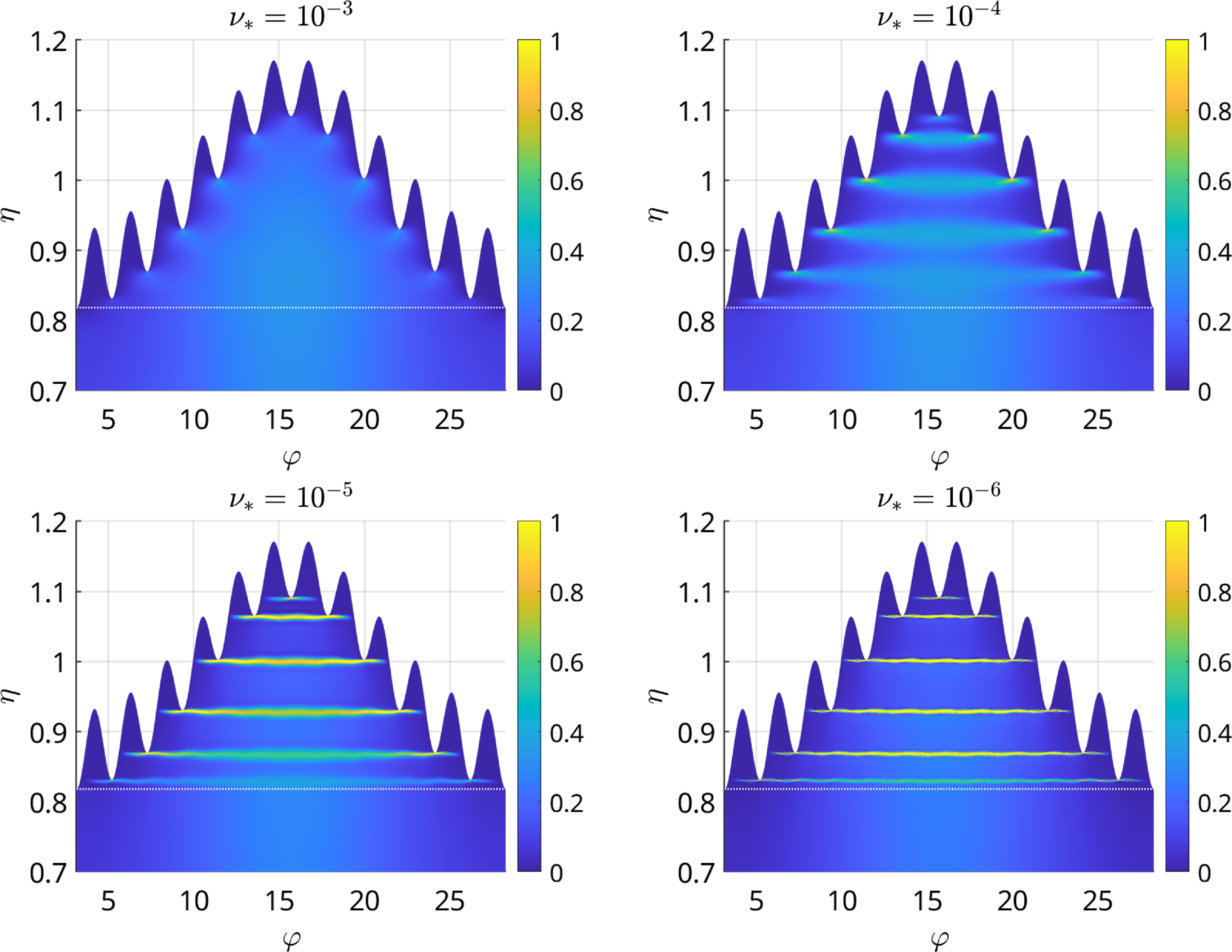
Figure 3. Odd part of the distribution function, $g^{\text{odd}}(\varphi, \eta )=(g(\varphi, \eta, 1)-g(\varphi, \eta, -1))/2$
, driven by
$g^{\text{odd}}(\varphi, \eta )=(g(\varphi, \eta, 1)-g(\varphi, \eta, -1))/2$
, driven by $s_{(1)}$
for different normalized collisionalities
$s_{(1)}$
for different normalized collisionalities $\nu _\ast$
(see the legend) in case
$\nu _\ast$
(see the legend) in case $\iota =1/4$
. The trapped–passing boundary is shown by a white dotted line.
$\iota =1/4$
. The trapped–passing boundary is shown by a white dotted line.
The distribution of the parallel equilibrium current in velocity space is better seen from figure 4, where an integral $\int _\eta ^{1/B} \textrm { d} \eta ^\prime \; g^{\text{odd}}$
is shown at the middle of the field line (
$\int _\eta ^{1/B} \textrm { d} \eta ^\prime \; g^{\text{odd}}$
is shown at the middle of the field line ( $\varphi =\varphi _b=5\pi$
). According to (2.38), the value of this integral at
$\varphi =\varphi _b=5\pi$
). According to (2.38), the value of this integral at $\eta =0$
up to a factor equals the parallel equilibrium current density. It can be seen that the contribution of the trapped particle region to the parallel current is independent of collisionality despite the varying width of the class-transition boundary layers which carry a significant amount of this current. Off-set of the current which depends on collisionality is produced in the passing particle region. Solution
$\eta =0$
up to a factor equals the parallel equilibrium current density. It can be seen that the contribution of the trapped particle region to the parallel current is independent of collisionality despite the varying width of the class-transition boundary layers which carry a significant amount of this current. Off-set of the current which depends on collisionality is produced in the passing particle region. Solution $g^{\text{odd}}$
in this region is determined up to arbitrary constant, which should match then the solution in the trapped–passing boundary layer. At sufficiently low collisionalities (
$g^{\text{odd}}$
in this region is determined up to arbitrary constant, which should match then the solution in the trapped–passing boundary layer. At sufficiently low collisionalities ( $\nu _\ast \lt 10^{-5}$
), where the bootstrap current is independent of collisionality, the nearest class-transition boundary layer is well separated from the trapped–passing boundary (see figure 5), and the boundary condition for passing particles is fully determined by the last trapped orbit nearest to the boundary between the trapped and passing particle domains (Boozer & Gardner Reference Boozer and Gardner1990). The rest of trapped particle domain has no effect on the passing distribution, because ‘particles’ generated by bounce-averaged drift in the first local ripple fully annihilate in class-transition boundary layer with ‘anti-particles’ generated in the last local ripple where the sign of geodesic curvature is opposite to the sign in the first ripple. At higher collisionalities (
$\nu _\ast \lt 10^{-5}$
), where the bootstrap current is independent of collisionality, the nearest class-transition boundary layer is well separated from the trapped–passing boundary (see figure 5), and the boundary condition for passing particles is fully determined by the last trapped orbit nearest to the boundary between the trapped and passing particle domains (Boozer & Gardner Reference Boozer and Gardner1990). The rest of trapped particle domain has no effect on the passing distribution, because ‘particles’ generated by bounce-averaged drift in the first local ripple fully annihilate in class-transition boundary layer with ‘anti-particles’ generated in the last local ripple where the sign of geodesic curvature is opposite to the sign in the first ripple. At higher collisionalities ( $\nu _\ast \geqslant 10^{-5}$
), where the trapped–passing boundary layer crosses the class-transition boundary, some part of the ‘particles’ generated in the first ripple (where source
$\nu _\ast \geqslant 10^{-5}$
), where the trapped–passing boundary layer crosses the class-transition boundary, some part of the ‘particles’ generated in the first ripple (where source $s_{(1)}\gt 0$
) and leaving this ripple with positive velocity (in the direction of a local maximum) when changing due to collisions their trapping class, can later cross the trapped–passing boundary without mirroring and enter a co-passing particle domain. Similarly, ‘anti-particles’ from the last ripple enter the counter-passing domain. Both create a current off-set of the same sign. Naturally, they cannot annihilate because they enter different domains.
$s_{(1)}\gt 0$
) and leaving this ripple with positive velocity (in the direction of a local maximum) when changing due to collisions their trapping class, can later cross the trapped–passing boundary without mirroring and enter a co-passing particle domain. Similarly, ‘anti-particles’ from the last ripple enter the counter-passing domain. Both create a current off-set of the same sign. Naturally, they cannot annihilate because they enter different domains.
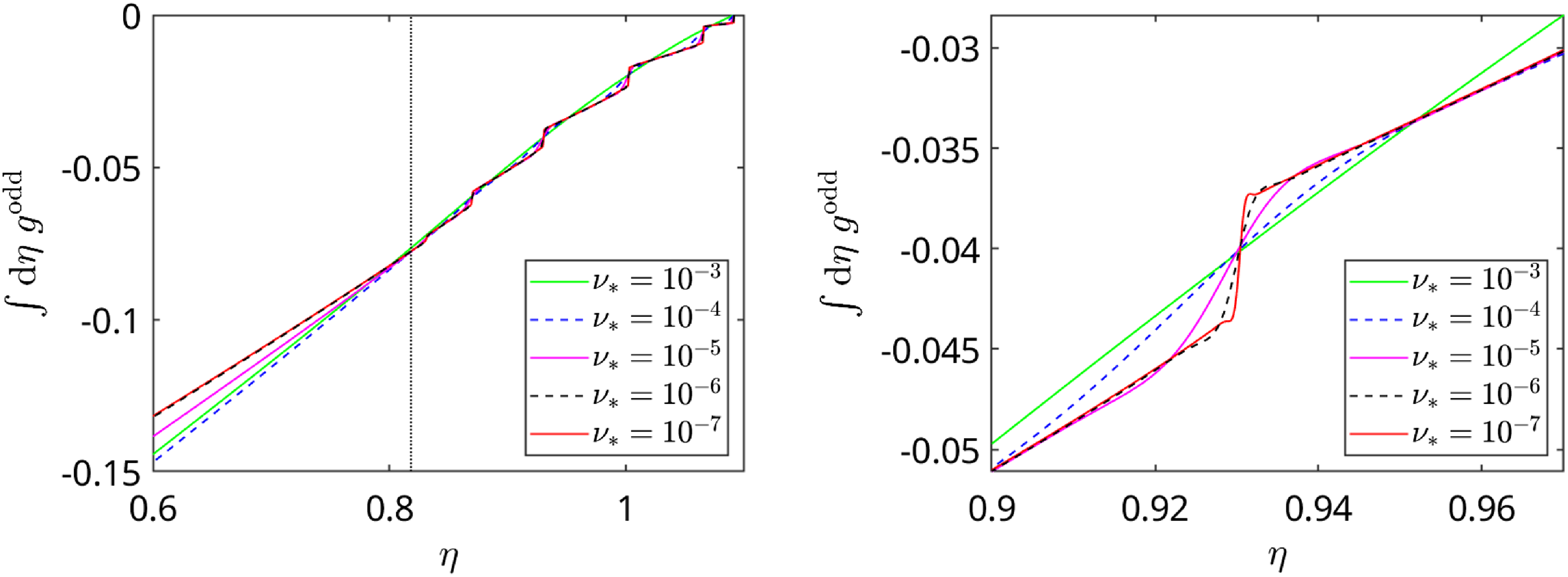
Figure 4. Integral $\int _\eta ^{1/B} \textrm { d} \eta ^\prime \; g^{\text{odd}}$
as a function of the lower limit (left), and its zoom near one of the class-transition boundaries (right) for various plasma collisionalities (see the legend) at
$\int _\eta ^{1/B} \textrm { d} \eta ^\prime \; g^{\text{odd}}$
as a function of the lower limit (left), and its zoom near one of the class-transition boundaries (right) for various plasma collisionalities (see the legend) at $\varphi =5\pi$
. The trapped–passing boundary is shown by a vertical dotted line.
$\varphi =5\pi$
. The trapped–passing boundary is shown by a vertical dotted line.
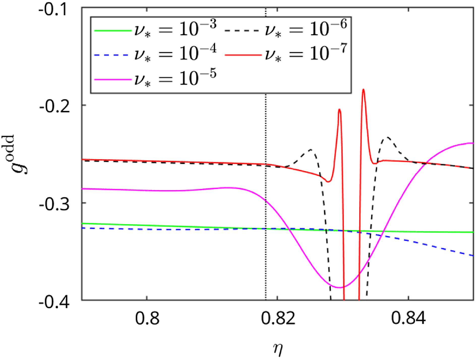
Figure 5. Odd part of the distribution function $g^{\text{odd}}$
near the trapped–passing boundary (vertical dotted line) at
$g^{\text{odd}}$
near the trapped–passing boundary (vertical dotted line) at $\varphi =5\pi$
for various collisionalities (see the legend).
$\varphi =5\pi$
for various collisionalities (see the legend).
Note that at some intermediate collisionality off-set changes sign (see figure 2). In this case, the class-transition layer is almost isolated from the trapped-passing boundary, so that the probability to enter the passing domain after a single pass along the boundary layer is lower than the probability to do that after the first reflection near the global maximum. In such a case, most ‘particles’ enter counter-passing domain (‘anti-particles’ – co-passing) which results in negative current off-set.
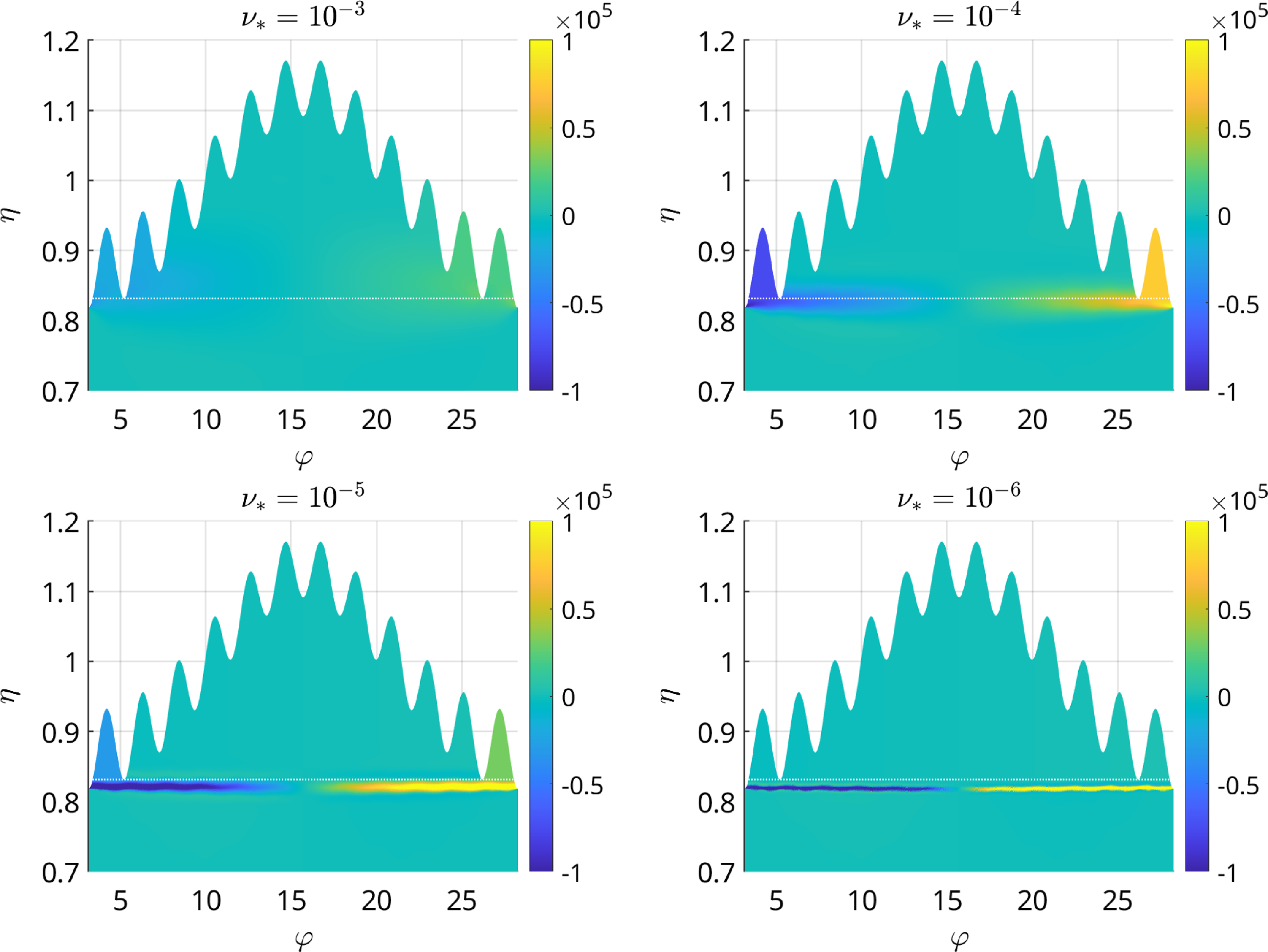
Figure 6. Even part of the distribution function, $g^{\text{even}}(\varphi, \eta )=(g(\varphi, \eta, 1)+g(\varphi, \eta, -1))/2$
, driven by
$g^{\text{even}}(\varphi, \eta )=(g(\varphi, \eta, 1)+g(\varphi, \eta, -1))/2$
, driven by $s_{(3)}$
for the same cases as in figure 3. The transition boundary between the two highest trapping classes is shown by a white dotted line.
$s_{(3)}$
for the same cases as in figure 3. The transition boundary between the two highest trapping classes is shown by a white dotted line.
2.3.2. Adjoint problem
An even part of the distribution function perturbation $g^{\text{even}}$
responsible for particle flux (Ware pinch) in the adjoint problem is shown in figure 6 for the same cases as in figure 3. As expected, the boundary layer appears at low collisionality only at the trapped–passing boundary. The structure of this layer well agrees with the complete analytical solution (2.53), i.e.
$g^{\text{even}}$
responsible for particle flux (Ware pinch) in the adjoint problem is shown in figure 6 for the same cases as in figure 3. As expected, the boundary layer appears at low collisionality only at the trapped–passing boundary. The structure of this layer well agrees with the complete analytical solution (2.53), i.e. $g^{\text{even}}$
is an anti-symmetric function of
$g^{\text{even}}$
is an anti-symmetric function of $\varphi$
with respect to the middle stellarator symmetry point
$\varphi$
with respect to the middle stellarator symmetry point $\varphi _s$
.
$\varphi _s$
.
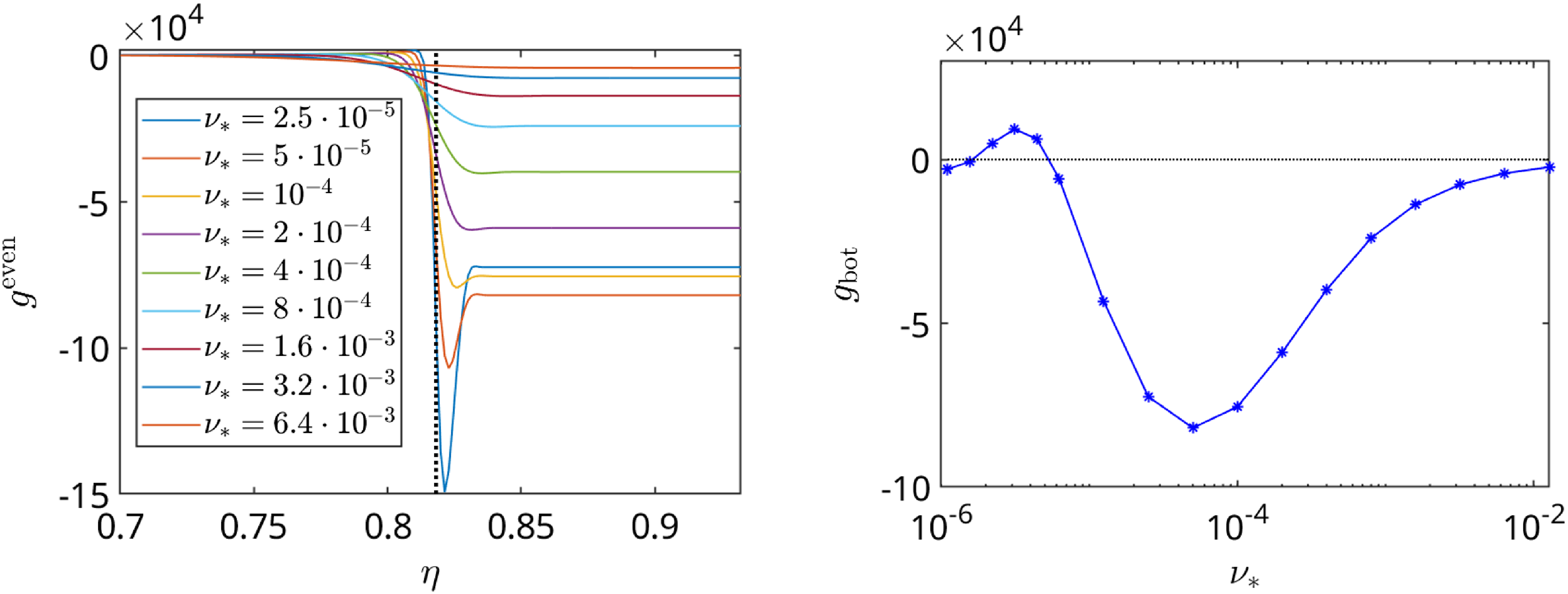
Figure 7. Even part of the distribution function $g^{\text{even}}$
as a function of
$g^{\text{even}}$
as a function of $\eta$
in the middle of the left off-set well,
$\eta$
in the middle of the left off-set well, $\varphi =4 \pi /3$
for various collisionalities (left) and
$\varphi =4 \pi /3$
for various collisionalities (left) and $\iota =1/4$
. The trapped–passing boundary is shown by a vertical dotted line. The value of
$\iota =1/4$
. The trapped–passing boundary is shown by a vertical dotted line. The value of $g^{\text{even}}$
at the off-set well bottom,
$g^{\text{even}}$
at the off-set well bottom, $g_{\text{bot}}$
, is shown as a function of
$g_{\text{bot}}$
, is shown as a function of $\nu _\ast$
in the right plot.
$\nu _\ast$
in the right plot.
Similar to the direct problem, if the trapped–passing boundary layer is well separated from the nearest class-transition boundary (lowest collisionality case, $\nu _\ast = 10^{-6}$
) the Ware-pinch coefficient agrees with the asymptotic limit. At higher collisionalities where this boundary layer enters a class-transition boundary, one can observe increased
$\nu _\ast = 10^{-6}$
) the Ware-pinch coefficient agrees with the asymptotic limit. At higher collisionalities where this boundary layer enters a class-transition boundary, one can observe increased $g^{\text{even}}$
in the local ripple wells whose lowest maximum determines this transition boundary. This accumulation of the particles in local ripples drives the off-set of Ware pinch since
$g^{\text{even}}$
in the local ripple wells whose lowest maximum determines this transition boundary. This accumulation of the particles in local ripples drives the off-set of Ware pinch since $g^{\text{even}}$
there is anti-symmetric with respect to the mid-point
$g^{\text{even}}$
there is anti-symmetric with respect to the mid-point $\varphi _b=5\pi$
, which is true also for geodesic curvature and, respectively, for the bounce-averaged radial drift velocity in these local ripples. Therefore, particles in both ripples drive the flux of the same sign. In the following, we will call such ripples ‘off-set wells’. As one can see from figure 7,
$\varphi _b=5\pi$
, which is true also for geodesic curvature and, respectively, for the bounce-averaged radial drift velocity in these local ripples. Therefore, particles in both ripples drive the flux of the same sign. In the following, we will call such ripples ‘off-set wells’. As one can see from figure 7, $g^{\text{even}}$
is constant in most of the off-set well, and changes only in the vicinity of class-transition boundary. Therefore, we can characterize
$g^{\text{even}}$
is constant in most of the off-set well, and changes only in the vicinity of class-transition boundary. Therefore, we can characterize $g^{\text{even}}$
in the whole off-set well by its value at the off-set well bottom, which will be denoted as
$g^{\text{even}}$
in the whole off-set well by its value at the off-set well bottom, which will be denoted as $g_{\text{off}}$
. It can be seen that
$g_{\text{off}}$
. It can be seen that $g_{\text{off}}$
has similar feature to
$g_{\text{off}}$
has similar feature to $\lambda _{bB}$
, i.e. it changes sign with reducing collisionality before going to zero.
$\lambda _{bB}$
, i.e. it changes sign with reducing collisionality before going to zero.

Figure 8. The same as in figure 6 for $\iota =2/5$
and different collisionalities (see the legend).
$\iota =2/5$
and different collisionalities (see the legend).
Properties of this distribution function off-set, which was also observed in GSRAKE modeling (Beidler Reference Beidler2020), will be studied in more detail in the next section. Here, we only show an extra example in figure 8 where more than one type of off-set wells is present simultaneously with different types of off-sets dominating at different collisionalities. In this example, both off-set wells containing only the lowest class of trapped particles who traverse a single minimum during their bounce period (as in figure 6) and an off-set wells containing many classes are shown. Note that trapped–passing boundary layer which has a standard (collisionless) form at lowest collisionality $\nu _\ast =10^{-6}$
appears to be split into two independent layers at the intermediate collisionalities
$\nu _\ast =10^{-6}$
appears to be split into two independent layers at the intermediate collisionalities $\nu _\ast \leqslant 10^{-4}$
where mismatch of two local maxima located near the middle of the field line with the global maximum becomes small compared with the typical boundary layer width (see the discussion of a few global maxima case after (2.53)). Thus, the off-set phenomenon has a rather high complexity even in the simple case of a closed field line which is, nevertheless, illustrative for realistic configurations. In particular, switching off-sets can be observed in figure 3 of Kernbichler et al. (Reference Kernbichler, Kasilov, Kapper, Martitsch, Nemov and Heyn2016) where bootstrap coefficient has been computed for W-7X down to collisionalities
$\nu _\ast \leqslant 10^{-4}$
where mismatch of two local maxima located near the middle of the field line with the global maximum becomes small compared with the typical boundary layer width (see the discussion of a few global maxima case after (2.53)). Thus, the off-set phenomenon has a rather high complexity even in the simple case of a closed field line which is, nevertheless, illustrative for realistic configurations. In particular, switching off-sets can be observed in figure 3 of Kernbichler et al. (Reference Kernbichler, Kasilov, Kapper, Martitsch, Nemov and Heyn2016) where bootstrap coefficient has been computed for W-7X down to collisionalities $\nu _\ast =10^{-9}$
.
$\nu _\ast =10^{-9}$
.
3. Bootstrap/Ware-pinch off-set for a closed field line
Let us study the bootstrap/Ware-pinch off-set phenomenon in more detail. Since both effects are quantitatively the same due to the Onsager symmetry of the transport coefficients, we focus now on the Ware-pinch effect only.
3.1. Boundary layer e-folding
As we have seen from asymptotic solutions and numerical examples in both direct and adjoint problems, the distribution function $g_0$
, which is independent of collisionality in most of the phase space, includes huge contributions localized in the boundary layers where they scale as
$g_0$
, which is independent of collisionality in most of the phase space, includes huge contributions localized in the boundary layers where they scale as $l_c^{1/2} \sim \nu ^{-1/2}$
and formally become infinite in the collisionless limit manifested by
$l_c^{1/2} \sim \nu ^{-1/2}$
and formally become infinite in the collisionless limit manifested by $\delta$
-functions in the asymptotic solutions. To estimate the decay of these localized contributions outside the boundary layer, we consider the homogeneous kinetic equation (2.3) and use the ansatz which is only slightly different from the ansatz of Helander et al. (Reference Helander, Geiger and Maassberg2011) and leads to the same approximation at the end. Namely, we replace in the trapped particle domain the independent variable
$\delta$
-functions in the asymptotic solutions. To estimate the decay of these localized contributions outside the boundary layer, we consider the homogeneous kinetic equation (2.3) and use the ansatz which is only slightly different from the ansatz of Helander et al. (Reference Helander, Geiger and Maassberg2011) and leads to the same approximation at the end. Namely, we replace in the trapped particle domain the independent variable $\varphi$
with
$\varphi$
with
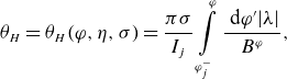 \begin{align} \theta _H = \theta _H(\varphi, \eta, \sigma ) = \frac {\pi \sigma }{I_j} \int \limits _{\varphi ^-_j}^\varphi \frac {\textrm { d} \varphi ^\prime |\lambda |}{ B^\varphi }, \end{align}
where the integral $I_j=I_j(\eta )$
is defined in (2.26). Thus, particles with
$I_j=I_j(\eta )$
is defined in (2.26). Thus, particles with $\lambda \gt 0$
are described by
$\lambda \gt 0$
are described by $0 \lt \theta _H \lt \pi$
, particles with
$0 \lt \theta _H \lt \pi$
, particles with $\lambda \lt 0$
are described by
$\lambda \lt 0$
are described by $-\pi \lt \theta _H \lt 0$
and continuity of the distribution function at both turning points is enabled by periodicity of
$-\pi \lt \theta _H \lt 0$
and continuity of the distribution function at both turning points is enabled by periodicity of $g$
with
$g$
with $\theta _H$
. Formally presenting the homogeneous equation (2.3) in tensor form
$\theta _H$
. Formally presenting the homogeneous equation (2.3) in tensor form
 \begin{align} \frac {\partial }{\partial z^i} \mathcal{J}\left (\mathcal{V}^i g- \mathcal{D}^{ij}\frac {\partial g}{\partial z^j}\right )=0, \end{align}
where $z^i=(\varphi, \eta )$
, and transforming the contra-variant components of the phase space velocity
$z^i=(\varphi, \eta )$
, and transforming the contra-variant components of the phase space velocity $\mathcal{V}^i$
and diffusion tensor
$\mathcal{V}^i$
and diffusion tensor $\mathcal{D}^{ij}$
and the Jacobian
$\mathcal{D}^{ij}$
and the Jacobian $\mathcal{J}$
to the new phase space coordinates
$\mathcal{J}$
to the new phase space coordinates $(\theta _H,\eta )$
using tensor algebra rules, this equation takes the form
$(\theta _H,\eta )$
using tensor algebra rules, this equation takes the form
 \begin{align} \frac {\partial g}{\partial \theta _H} = \left (\frac {\partial }{\partial \eta } +\frac {\partial }{\partial \theta _H} \frac {\partial \theta _H}{\partial \eta }\right ) D_H \left (\frac {\partial g}{\partial \eta } + \frac {\partial \theta _H}{\partial \eta }\frac {\partial g}{\partial \theta _H}\right ), \end{align}
where differential operators $\partial /\partial \eta$
and
$\partial /\partial \eta$
and $\partial /\partial \theta _H$
act on everything to the right, and
$\partial /\partial \theta _H$
act on everything to the right, and
 \begin{align} D_H = D_H(\eta ) = \frac {\eta I_j}{\pi l_c}. \end{align}
Expanding the distribution function in Fourier series over $\theta _H$
,
$\theta _H$
,
 \begin{align} g(\theta _H,\eta )=\sum \limits _{m=-\infty }^\infty g_{[m]}\textrm { e}^{i m \theta _H}, \end{align}
equation (3.3) turns into a coupled set of ordinary differential equations for Fourier amplitudes $g_{[m]}(\eta )$
. It should be noted that terms with
$g_{[m]}(\eta )$
. It should be noted that terms with $\partial \theta _H / \partial \eta$
which lead to the coupling of Fourier modes are negligibly small in most of phase space except for the close vicinity of the boundary (sub-layer (Helander et al. Reference Helander, Geiger and Maassberg2011)) where due to the scaling
$\partial \theta _H / \partial \eta$
which lead to the coupling of Fourier modes are negligibly small in most of phase space except for the close vicinity of the boundary (sub-layer (Helander et al. Reference Helander, Geiger and Maassberg2011)) where due to the scaling $\partial ^2 \theta _H / \partial \eta ^2 \sim \eta ^{-1} (\eta -\eta _b)^{-1}$
their contribution is comparable to the left-hand side which means the sub-layer width
$\partial ^2 \theta _H / \partial \eta ^2 \sim \eta ^{-1} (\eta -\eta _b)^{-1}$
their contribution is comparable to the left-hand side which means the sub-layer width $\eta -\eta _b \sim \nu _\ast \ll \sqrt {\nu _\ast }$
. Thus, one can ignore the right-hand side terms with derivatives over
$\eta -\eta _b \sim \nu _\ast \ll \sqrt {\nu _\ast }$
. Thus, one can ignore the right-hand side terms with derivatives over $\theta _H$
outside the sub-layer, and the set decouples into
$\theta _H$
outside the sub-layer, and the set decouples into
 \begin{align} im g_{[m]} = \frac {\partial }{\partial \eta }D_H\frac {\partial g_{[m]}}{\partial \eta }. \end{align}
Harmonic
 \begin{align} g_{[0]} = \frac {1}{2 I_j}\sum _{\sigma = \pm 1} \int \limits _{\varphi ^-_j}^{\varphi ^+_j}\textrm { d} \varphi \frac {|\lambda |g}{B^\varphi }, \end{align}
is actually zero in our case because $\delta$
-like terms in the direct problem are odd, and the solution of the adjoint problem is stellarator antisymmetric. Ignoring in (3.6), variation of
$\delta$
-like terms in the direct problem are odd, and the solution of the adjoint problem is stellarator antisymmetric. Ignoring in (3.6), variation of $D_H$
in the main boundary layer,
$D_H$
in the main boundary layer, $D_H(\eta ) \approx D_H(\eta _b)$
, which brings this equation in agreement with the result of the “rectangular well” ansatz of Helander et al. (Reference Helander, Geiger and Maassberg2011), we look for solutions in the form
$D_H(\eta ) \approx D_H(\eta _b)$
, which brings this equation in agreement with the result of the “rectangular well” ansatz of Helander et al. (Reference Helander, Geiger and Maassberg2011), we look for solutions in the form $g_{[m]} \propto \exp (\kappa _m (\eta -\eta _b))$
with the
$g_{[m]} \propto \exp (\kappa _m (\eta -\eta _b))$
with the $m=1$
harmonic being dominant with increasing
$m=1$
harmonic being dominant with increasing $\eta -\eta _b$
. Thus, boundary layer contribution decays outside the layer as
$\eta -\eta _b$
. Thus, boundary layer contribution decays outside the layer as
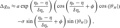 \begin{align} \Delta g_{\text {fit}} & \approx a \exp \left (\frac {\eta _b-\eta }{\delta \eta _e}\right ) \left ( \cos \left (\frac {\eta _b-\eta }{\delta \eta _e}+\phi \right ) \cos \left (|\theta _H|\right ) \right. \nonumber\\ & \left. \quad - \sigma \sin \left (\frac {\eta _b-\eta }{\delta \eta _e}+\phi \right ) \sin \left (|\theta _H|\right ) \right ), \end{align}
where $|\theta _H|=|\theta _H(\varphi, \eta )|$
, and
$|\theta _H|=|\theta _H(\varphi, \eta )|$
, and $\delta \eta _e$
is boundary layer e-folding length,
$\delta \eta _e$
is boundary layer e-folding length,
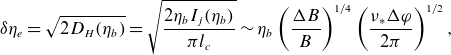 \begin{align} \delta \eta _e = \sqrt {2 D_H(\eta _b)} = \sqrt {\frac {2 \eta _b I_j(\eta _b)}{\pi l_c}} \sim \eta _b \left (\frac {\Delta B}{B}\right )^{1/4} \left (\frac {\nu _\ast \Delta \varphi }{2\pi }\right )^{1/2}, \end{align}
estimated in the last expression via typical variation of $B$
in the magnetic well
$B$
in the magnetic well $\Delta B$
and toroidal extent of the boundary layer
$\Delta B$
and toroidal extent of the boundary layer $\Delta \varphi$
.
$\Delta \varphi$
.
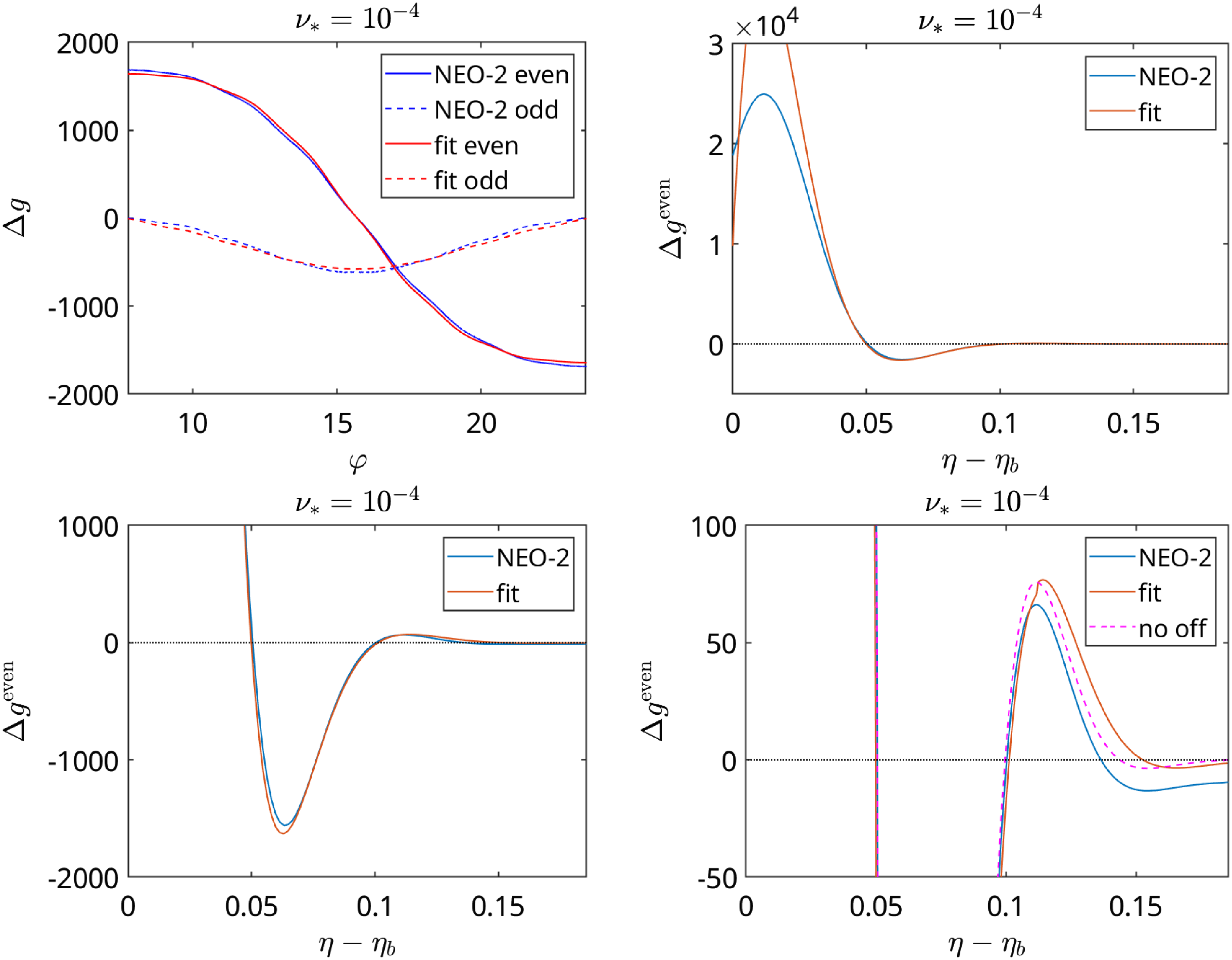
Figure 9. Difference $\Delta g$
and the fit
$\Delta g$
and the fit $\Delta g_{\text{fit}}$
, (3.8) for the case
$\Delta g_{\text{fit}}$
, (3.8) for the case $\nu _\ast =10^{-4}$
in figure 6. Upper left – even and odd parts as functions of
$\nu _\ast =10^{-4}$
in figure 6. Upper left – even and odd parts as functions of $\varphi$
for
$\varphi$
for $\eta -\eta _b=0.07$
. Upper right – even parts as functions of
$\eta -\eta _b=0.07$
. Upper right – even parts as functions of $\eta$
for
$\eta$
for $\varphi =19 \pi /3$
(7th local maximum). Lower panel – zooms of the upper right plot over the Y-axis. Dashed line in the last zoom corresponds to the NEO-2 result for
$\varphi =19 \pi /3$
(7th local maximum). Lower panel – zooms of the upper right plot over the Y-axis. Dashed line in the last zoom corresponds to the NEO-2 result for $g^{\text{even}}-g_{\lambda =0}$
, where
$g^{\text{even}}-g_{\lambda =0}$
, where $g_{\lambda =0}$
is
$g_{\lambda =0}$
is $g^{\text{even}}$
for standing particles with
$g^{\text{even}}$
for standing particles with $\eta =1/B$
. Function
$\eta =1/B$
. Function $g_{\lambda =0}$
differs here from
$g_{\lambda =0}$
differs here from $g_0=g_0^t$
by an exponentially small off-set.
$g_0=g_0^t$
by an exponentially small off-set.
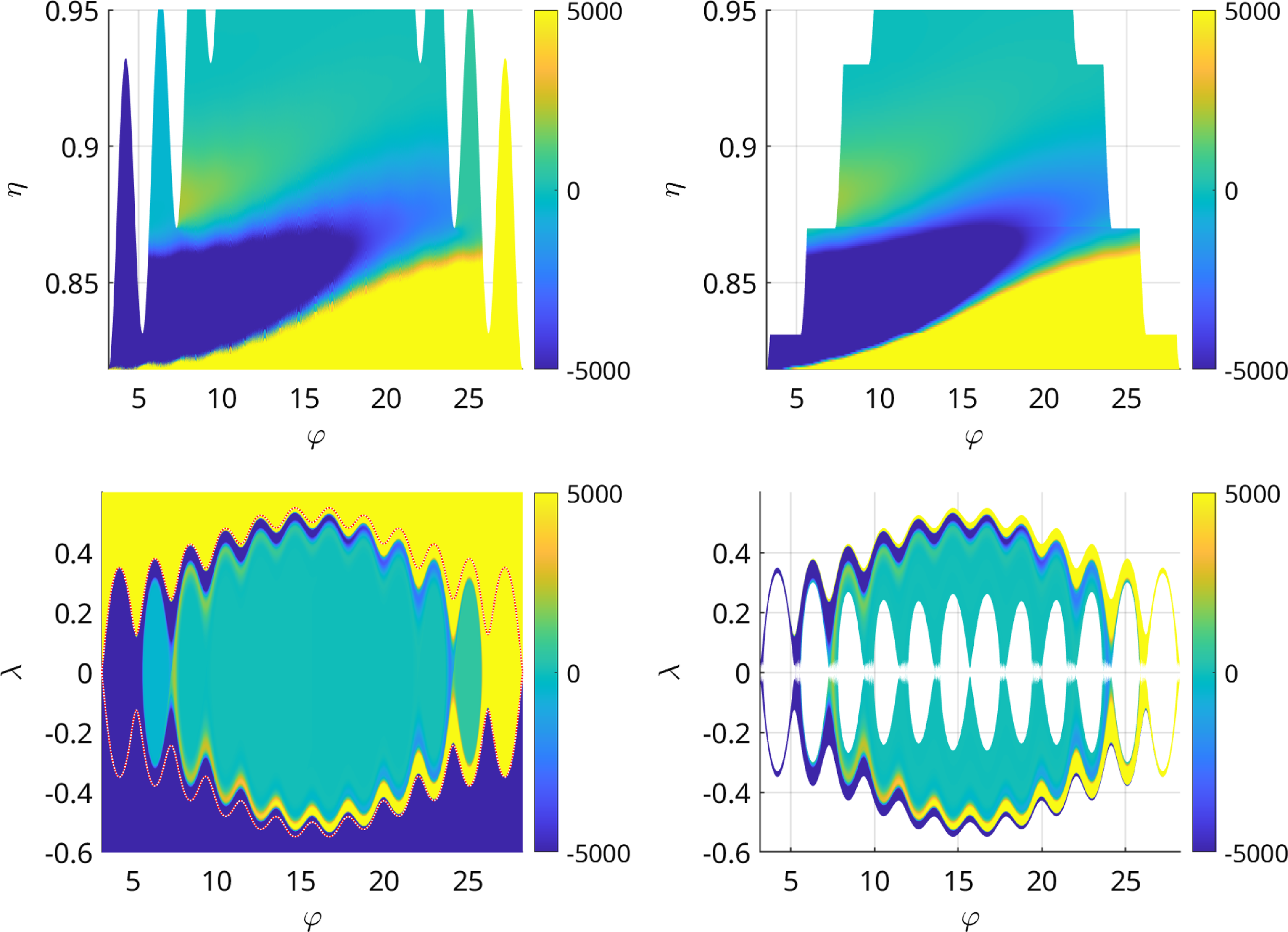
Figure 10. Difference $\Delta g$
(left) and its fit
$\Delta g$
(left) and its fit $\Delta g_{\text{fit}}$
(right) as functions of
$\Delta g_{\text{fit}}$
(right) as functions of $(\varphi, \eta )$
and
$(\varphi, \eta )$
and $\sigma =1$
(upper panel) and
$\sigma =1$
(upper panel) and $(\varphi, \lambda )$
(lower panel) for the same case as in figure 9. Saturation of color scale at
$(\varphi, \lambda )$
(lower panel) for the same case as in figure 9. Saturation of color scale at $|\Delta g| \geqslant 5000$
occurs in the whole passing particle region. Fit
$|\Delta g| \geqslant 5000$
occurs in the whole passing particle region. Fit $\Delta g_{\text{fit}}$
is plotted excluding passing particle domains and local trapping domains where
$\Delta g_{\text{fit}}$
is plotted excluding passing particle domains and local trapping domains where $\Delta g_{\text{fit}}$
is not defined. Red dotted line in
$\Delta g_{\text{fit}}$
is not defined. Red dotted line in $\Delta g(\varphi, \lambda )$
plot shows the trapped–passing boundary where transient particles move clockwise.
$\Delta g(\varphi, \lambda )$
plot shows the trapped–passing boundary where transient particles move clockwise.
In figures 9 and 10, the boundary layer contribution represented by the difference $\Delta g = g-g_0$
between the numerical (NEO-2) and analytical (2.47) solutions of the adjoint problem is compared with the asymptotic boundary layer solution
$\Delta g = g-g_0$
between the numerical (NEO-2) and analytical (2.47) solutions of the adjoint problem is compared with the asymptotic boundary layer solution $\Delta g_{\text{fit}}$
given by (3.8) with amplitude
$\Delta g_{\text{fit}}$
given by (3.8) with amplitude $a$
and phase
$a$
and phase $\phi$
fitted to match
$\phi$
fitted to match $\Delta g$
in the upper left plot of figure 9. Oscillations of
$\Delta g$
in the upper left plot of figure 9. Oscillations of $\Delta g$
with
$\Delta g$
with $\eta$
in figure 9 result from interchanging dominance of “particles’ and “anti-particles” which enter the trapping domain and become mirrored there once (twice, etc.). Since the observation point in the last three plots is in the region
$\eta$
in figure 9 result from interchanging dominance of “particles’ and “anti-particles” which enter the trapping domain and become mirrored there once (twice, etc.). Since the observation point in the last three plots is in the region $\varphi _s\lt \varphi \lt \varphi _N$
, “particles” dominate there over “anti-particles” in the first peak (see also figure 6) which they produce before the first reflection. The above mechanism results in helical structures in
$\varphi _s\lt \varphi \lt \varphi _N$
, “particles” dominate there over “anti-particles” in the first peak (see also figure 6) which they produce before the first reflection. The above mechanism results in helical structures in $g(\varphi, \lambda )$
distribution formed in the trapped particle domain (see figure 10). They are produced by the combination of the collisionless phase space flow (which is clockwise in this domain) and the flow driven by the collisional diffusion (directed over
$g(\varphi, \lambda )$
distribution formed in the trapped particle domain (see figure 10). They are produced by the combination of the collisionless phase space flow (which is clockwise in this domain) and the flow driven by the collisional diffusion (directed over $\lambda$
to the trapped particle domain from the co- and counter-passing particle domains, where sources of “particles” and “anti-particles” are located, respectively).
$\lambda$
to the trapped particle domain from the co- and counter-passing particle domains, where sources of “particles” and “anti-particles” are located, respectively).
Note that oscillatory behavior similar to that in figure 9 is seen also in the class-transition boundary layers in figure 5 and is reflected then in the small bootstrap off-set oscillation in figure 2 at low collisionality, where it decreases exponentially.
3.2. Propagator method, leading-order solution
For more detailed analysis of boundary layer effects on bootstrap/Ware-pinch off-set, we use propagator method. We look for the solution of the adjoint problem in the whole phase space in the form
 \begin{align} g_{(3)}(\varphi, \eta, \sigma ) = \Theta (\eta _b-\eta )g_{-1}(\eta )+g_0^{t}(\varphi )+g_{\text{bou}}(\varphi, \eta, \sigma ), \end{align}
where $g_{-1}$
and
$g_{-1}$
and $g_0^{t}$
are given by (2.46) and (2.47), respectively. The kinetic equation (2.3) corresponding to the source
$g_0^{t}$
are given by (2.46) and (2.47), respectively. The kinetic equation (2.3) corresponding to the source $s_{(3)}$
transforms to
$s_{(3)}$
transforms to
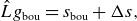 \begin{align} \hat L g_{\text{bou}} = s_{\text{bou}} + \Delta s, \end{align}
where the source terms are
 \begin{align} s_{\text{bou}} = \sigma l_c \delta (\eta _b-\eta ) \frac {D_\eta \langle B^2 \rangle }{\langle |\lambda | \rangle }, \\[-24pt] \nonumber \end{align}
 \begin{align} \Delta s = -\sigma l_c \Theta (\eta _b-\eta ) \frac {\partial }{\partial \eta } \frac {D_\eta \langle B^2 \rangle }{\langle |\lambda | \rangle } - \sigma l_c \frac {\partial }{\partial \eta }\left ( \delta (\eta _b-\eta ) D_\eta \int \limits _\eta ^{\eta _b} \textrm { d} \eta ^\prime \frac {\langle B^2 \rangle }{\langle |\lambda | \rangle } \right ). \end{align}
In the following, we use a formal solution of (3.11) in terms of its Green’s function, which makes it evident that the last term in (3.13) does not contribute to the solution since $\eta$
-integral of this term weighted with any function with finite derivative over
$\eta$
-integral of this term weighted with any function with finite derivative over $\eta$
is zero. The remaining term, as we check later, provides a correction of the order
$\eta$
is zero. The remaining term, as we check later, provides a correction of the order $\delta \eta _e$
to the solution driven by
$\delta \eta _e$
to the solution driven by $s_{\text{bou}}$
, (3.12). Thus, we ignore
$s_{\text{bou}}$
, (3.12). Thus, we ignore $\Delta s$
fully in the leading-order solution. Note that
$\Delta s$
fully in the leading-order solution. Note that $g_{\text{bou}}$
is an aperiodic function in the passing region due to aperiodicity of
$g_{\text{bou}}$
is an aperiodic function in the passing region due to aperiodicity of $g_o^t$
in the definition (3.10). The leading-order solution is treated nevertheless as periodic, with the aperiodic term included in the ignored correction driven by
$g_o^t$
in the definition (3.10). The leading-order solution is treated nevertheless as periodic, with the aperiodic term included in the ignored correction driven by $\Delta s$
. It should be noted that correction terms ignored here may become important in a special case where the leading-order solution tends to vanish. These cases are discussed below in §§ 3.3 and 4.3.
$\Delta s$
. It should be noted that correction terms ignored here may become important in a special case where the leading-order solution tends to vanish. These cases are discussed below in §§ 3.3 and 4.3.
We make the following simplifications. As follows from the analysis in § 3.1, solutions driven by sources located in the passing region or at the trapped–passing boundary tend exponentially to constants of $\eta$
at some sufficiently large distance from the trapped–passing boundary,
$\eta$
at some sufficiently large distance from the trapped–passing boundary, $\eta \gt \eta _m$
, where matching boundary
$\eta \gt \eta _m$
, where matching boundary $\eta _m$
satisfies
$\eta _m$
satisfies $\delta \eta _e \ll \eta _m -\eta _b \ll \eta _b$
. Generally, these constants can be different in different ripple wells in case they are bounded on both sides by the maxima fulfilling
$\delta \eta _e \ll \eta _m -\eta _b \ll \eta _b$
. Generally, these constants can be different in different ripple wells in case they are bounded on both sides by the maxima fulfilling $\eta _m B(\varphi _j)\gt 1$
, see figures 6 and 7. Thus, we solve (3.11) only in the domain
$\eta _m B(\varphi _j)\gt 1$
, see figures 6 and 7. Thus, we solve (3.11) only in the domain $\eta \lt \eta _m$
imposing at the matching boundary zero flux condition,
$\eta \lt \eta _m$
imposing at the matching boundary zero flux condition, $\partial g_{\text {bou}}(\varphi, \eta _m,\sigma ) / \partial \eta _m=0$
. The boundary
$\partial g_{\text {bou}}(\varphi, \eta _m,\sigma ) / \partial \eta _m=0$
. The boundary $\eta =\eta _m$
serves then as an upper boundary in most trapped particle domain, except the interface regions near the global maximum and local maxima fulfilling
$\eta =\eta _m$
serves then as an upper boundary in most trapped particle domain, except the interface regions near the global maximum and local maxima fulfilling $\eta _m B(\varphi _j) \gt 1$
, where
$\eta _m B(\varphi _j) \gt 1$
, where $\eta _m B(\varphi ) \gt 1$
, see figure 11. Since the widths of these regions
$\eta _m B(\varphi ) \gt 1$
, see figure 11. Since the widths of these regions $\delta \varphi$
are small at low collisionalities,
$\delta \varphi$
are small at low collisionalities, $\delta \varphi \sim B\delta \eta _e^{1/2}\left (\partial ^2 B / \partial \varphi ^2\right )^{-1/2} \propto l_c^{-1/4}$
, we ignore the collision and source terms there, which leads in such a leading-order solution to an error of the order
$\delta \varphi \sim B\delta \eta _e^{1/2}\left (\partial ^2 B / \partial \varphi ^2\right )^{-1/2} \propto l_c^{-1/4}$
, we ignore the collision and source terms there, which leads in such a leading-order solution to an error of the order $|\lambda |\delta \varphi \sim (\delta \eta _e B)^{1/2} \delta \varphi \sim \delta \eta _e B^{3/2} \left (\partial ^2 B / \partial \varphi ^2\right )^{-1/2} \propto l_c^{-1/2}$
, being of the same order as an error introduced by ignoring the sub-layer in § 3.1. (For this error estimate in the main boundary layer,
$|\lambda |\delta \varphi \sim (\delta \eta _e B)^{1/2} \delta \varphi \sim \delta \eta _e B^{3/2} \left (\partial ^2 B / \partial \varphi ^2\right )^{-1/2} \propto l_c^{-1/2}$
, being of the same order as an error introduced by ignoring the sub-layer in § 3.1. (For this error estimate in the main boundary layer, $|\eta -\eta _b| \sim \delta \eta _e$
, we compared the variance
$|\eta -\eta _b| \sim \delta \eta _e$
, we compared the variance $2\int \textrm { d}\varphi D_\eta$
in particle
$2\int \textrm { d}\varphi D_\eta$
in particle $\eta$
introduced by the collisions when traversing the interface region with such variance for the whole trapping region assuming in the latter for simplicity that both,
$\eta$
introduced by the collisions when traversing the interface region with such variance for the whole trapping region assuming in the latter for simplicity that both, $\lambda$
and the region extent in
$\lambda$
and the region extent in $\varphi$
are of the order one. The error of the above model is of the order of one within the sub-layers, where effect of collisions on
$\varphi$
are of the order one. The error of the above model is of the order of one within the sub-layers, where effect of collisions on $\lambda$
becomes comparable to the effect of mirroring force, but the overall contribution of these narrow sub-layers is similarly small.)
$\lambda$
becomes comparable to the effect of mirroring force, but the overall contribution of these narrow sub-layers is similarly small.)
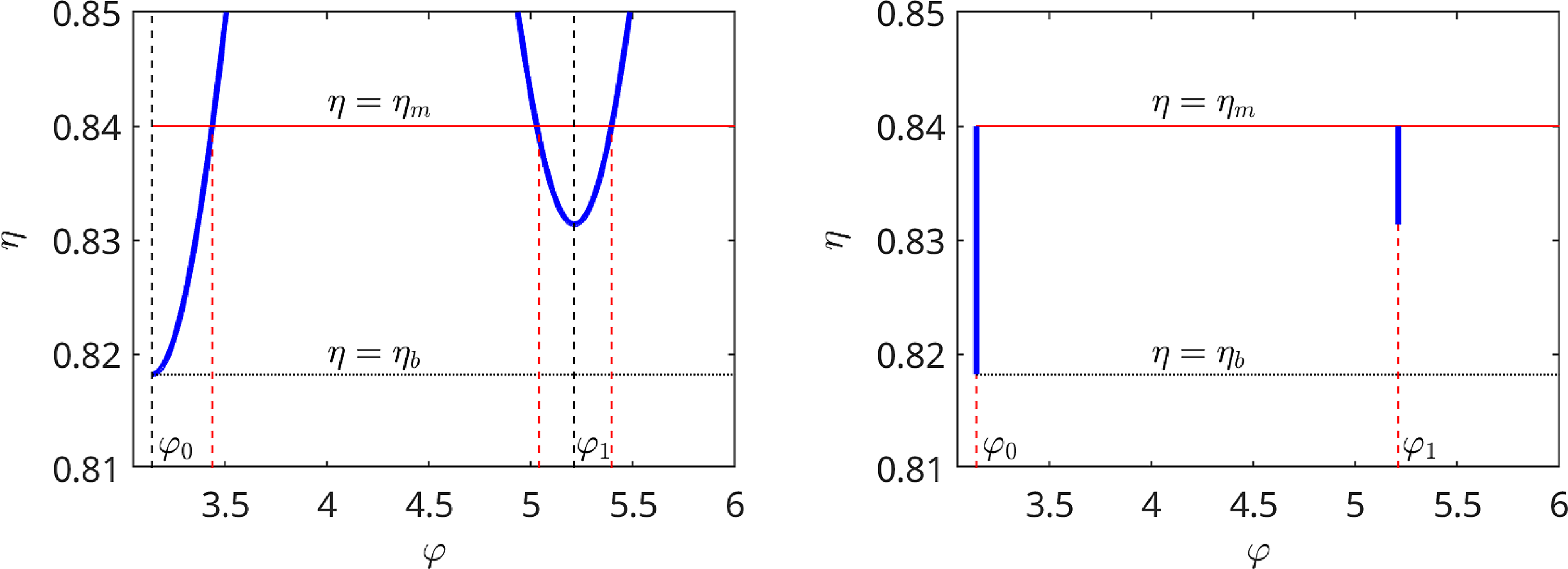
Figure 11. Computation domain before (left) and after (right) simplifying transformation. Trapped–passing boundary $\eta =\eta _b$
and matching boundary
$\eta =\eta _b$
and matching boundary $\eta =\eta _m$
are shown by black dotted and red solid line, respectively. Original domain boundary
$\eta =\eta _m$
are shown by black dotted and red solid line, respectively. Original domain boundary $\eta =1/B(\varphi )$
(solid blue), field maxima
$\eta =1/B(\varphi )$
(solid blue), field maxima $\varphi _j$
(dashed black) and boundaries of interface regions
$\varphi _j$
(dashed black) and boundaries of interface regions $\varphi _j \pm \delta \varphi$
(dashed red) are shown in the left plot. Reflecting (solid) and transparent (dashed) boundaries of the transformed domain are shown in the right plot.
$\varphi _j \pm \delta \varphi$
(dashed red) are shown in the left plot. Reflecting (solid) and transparent (dashed) boundaries of the transformed domain are shown in the right plot.
The solution is trivial in the interface regions, and we can express it via mapping between the boundaries $\varphi _j \pm \delta \varphi$
where
$\varphi _j \pm \delta \varphi$
where $\varphi _j$
is maximum point
$\varphi _j$
is maximum point
 \begin{eqnarray} g_{\text{bou}}(\varphi _j \pm \delta \varphi, \eta, \pm 1)\;&=&\; g_{\text{bou}}(\varphi _j \mp \delta \varphi, \eta, \pm 1), \qquad \eta B(\varphi _j) \lt 1, \nonumber \\ g_{\text{bou}}(\varphi _j \pm \delta \varphi, \eta, \pm 1)\;&=&\; g_{\text{bou}}(\varphi _j \pm \delta \varphi, \eta, \mp 1), \qquad \eta B(\varphi _j) \gt 1. \end{eqnarray}
Similar to § 3.1, we ignore the dependence of the diffusion coefficient on $\eta$
, setting
$\eta$
, setting $D_\eta (\varphi, \eta ) \rightarrow D_\eta (\varphi, \eta _b)$
and, finally, ignore the extent of interface regions,
$D_\eta (\varphi, \eta ) \rightarrow D_\eta (\varphi, \eta _b)$
and, finally, ignore the extent of interface regions, $\delta \varphi \rightarrow 0$
, with each of these steps introducing an error of the order
$\delta \varphi \rightarrow 0$
, with each of these steps introducing an error of the order $B\delta \eta _c \sim l_c^{-1/2}$
, as before. Thus, we have transformed our computation domain to a set of rectangular domains
$B\delta \eta _c \sim l_c^{-1/2}$
, as before. Thus, we have transformed our computation domain to a set of rectangular domains $0\lt \eta \lt \eta _m$
,
$0\lt \eta \lt \eta _m$
, $\varphi _j \lt \varphi \lt \varphi _{j+1}$
, limited by relevant field maxima,
$\varphi _j \lt \varphi \lt \varphi _{j+1}$
, limited by relevant field maxima, $\eta _m B(\varphi _j) \gt 1$
(see figure 11). This transformation leads to similar simplifications of the kinetic equation as the transformation used in § 3.1 for the main trapping region (or for the whole field line in case of vanishing boundary layer width) and is the same as the transformation of Helander et al. (Reference Helander, Geiger and Maassberg2011) extended here to multiple local trapping regions.
$\eta _m B(\varphi _j) \gt 1$
(see figure 11). This transformation leads to similar simplifications of the kinetic equation as the transformation used in § 3.1 for the main trapping region (or for the whole field line in case of vanishing boundary layer width) and is the same as the transformation of Helander et al. (Reference Helander, Geiger and Maassberg2011) extended here to multiple local trapping regions.
Introducing Green’s function $G_\sigma (\varphi, \eta, \varphi ^\prime, \eta ^\prime )$
which satisfies, with respect to
$G_\sigma (\varphi, \eta, \varphi ^\prime, \eta ^\prime )$
which satisfies, with respect to $(\varphi, \eta )$
variables, the homogeneous equation (3.11) with
$(\varphi, \eta )$
variables, the homogeneous equation (3.11) with $D_\eta =D_\eta (\varphi, \eta _b)$
, boundary conditions at the strongly passing and the matching boundary
$D_\eta =D_\eta (\varphi, \eta _b)$
, boundary conditions at the strongly passing and the matching boundary
 \begin{align} \left (\frac {\partial }{\partial \eta } G_\sigma (\varphi, \eta, \varphi ^\prime, \eta ^\prime )\right )_{\eta =0} = \left (\frac {\partial }{\partial \eta } G_\sigma (\varphi, \eta, \varphi ^\prime, \eta ^\prime )\right )_{\eta =\eta _m} =0, \end{align}
and initial condition $G_\sigma (\varphi ^\prime, \eta, \varphi ^\prime, \eta ^\prime )=\delta (\eta -\eta ^\prime )$
at the starting point
$G_\sigma (\varphi ^\prime, \eta, \varphi ^\prime, \eta ^\prime )=\delta (\eta -\eta ^\prime )$
at the starting point $\varphi ^\prime$
, we can formally express the leading-order solution to (3.11) within a single trapping domain,
$\varphi ^\prime$
, we can formally express the leading-order solution to (3.11) within a single trapping domain, $\varphi _j\lt \varphi, \varphi ^\prime \lt \varphi _{j+1}$
, as
$\varphi _j\lt \varphi, \varphi ^\prime \lt \varphi _{j+1}$
, as
 \begin{align} g_{\text{bou}}(\varphi, \eta, \sigma ) = \int \limits _0^{\eta _m}\textrm { d}\eta ^\prime G_\sigma (\varphi, \eta, \varphi ^\prime, \eta ^\prime ) g_{\text{bou}}(\varphi ^\prime, \eta ^\prime, \sigma ) + Q_\sigma (\varphi, \varphi ^\prime, \eta ), \end{align}
where $\varphi \gt \varphi ^\prime$
for
$\varphi \gt \varphi ^\prime$
for $\sigma =1$
and
$\sigma =1$
and $\varphi \lt \varphi ^\prime$
for
$\varphi \lt \varphi ^\prime$
for $\sigma =-1$
, and where
$\sigma =-1$
, and where
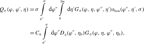 \begin{eqnarray} Q_\sigma (\varphi, \varphi ^\prime, \eta ) \;&=&\; \sigma \int \limits _{\varphi ^\prime }^\varphi \textrm { d}\varphi ^{\prime \prime } \int \limits _0^{\eta _m}\textrm { d}\eta ^\prime G_\sigma (\varphi, \eta, \varphi ^{\prime \prime },\eta ^\prime ) s_{\text{bou}}(\varphi ^{\prime \prime },\eta ^\prime, \sigma ) \nonumber \\ &=&\; C_0 \int \limits _{\varphi ^\prime }^\varphi \textrm { d}\varphi ^{\prime \prime } D_\eta (\varphi ^{\prime \prime },\eta _b) G_\sigma (\varphi, \eta, \varphi ^{\prime \prime },\eta _b), \end{eqnarray}
with a constant
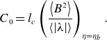 \begin{align} C_0 = l_c\left (\frac {\left \langle B^2\right \rangle } {\langle |\lambda |\rangle }\right )_{\eta =\eta _b}. \end{align}
Introducing the fundamental solution in the unbounded $\eta$
-region
$\eta$
-region
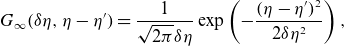 \begin{align} G_\infty (\delta \eta, \eta -\eta ^\prime )=\frac {1}{\sqrt {2\pi } \delta \eta } \exp \left ({-}\frac {(\eta -\eta ^\prime )^2}{2\delta \eta ^2}\right ), \end{align}
where
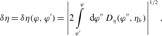 \begin{align} \delta \eta = \delta \eta (\varphi, \varphi ^\prime ) = \left |2\int \limits _{\varphi ^\prime }^{\varphi }\textrm { d} \varphi ^{\prime \prime }\; D_\eta (\varphi ^{\prime \prime },\eta _b)\right |^{1/2}, \end{align}
we can construct Green’s function satisfying boundary conditions (3.15) as
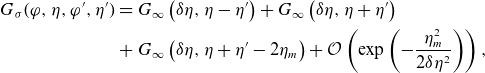 \begin{eqnarray} G_\sigma (\varphi, \eta, \varphi ^\prime, \eta ^\prime ) \;&=&\; G_\infty \left (\delta \eta, \eta -\eta ^\prime \right ) + G_\infty \left (\delta \eta, \eta +\eta ^\prime \right ) \nonumber \\ &+&\; G_\infty \left (\delta \eta, \eta +\eta ^\prime -2\eta _m\right ) +\mathcal{O}\left (\exp \left ({-}\frac {\eta _m^2}{2 \delta \eta ^2}\right )\right ), \end{eqnarray}
with the last term being negligibly small in the long mean free path regime where $\delta \eta \ll \eta _m$
. By our assumption,
$\delta \eta \ll \eta _m$
. By our assumption, $\delta \eta \lt \delta \eta _e \ll (\eta _m-\eta _b)$
, and, of course,
$\delta \eta \lt \delta \eta _e \ll (\eta _m-\eta _b)$
, and, of course, $\delta \eta \ll \eta _b$
. Therefore, the second and third terms in (3.21) provide similarly exponentially small contributions to the source term (3.17) which can be expressed then as
$\delta \eta \ll \eta _b$
. Therefore, the second and third terms in (3.21) provide similarly exponentially small contributions to the source term (3.17) which can be expressed then as
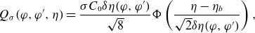 \begin{align} Q_\sigma (\varphi, \varphi ^\prime, \eta )=\frac {\sigma C_0\delta \eta (\varphi, \varphi ^\prime )}{\sqrt {8}} \Phi \left (\frac {\eta -\eta _b}{\sqrt {2}\delta \eta (\varphi, \varphi ^\prime )}\right ), \end{align}
where
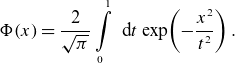 \begin{align} \Phi (x)=\frac {2}{\sqrt {\pi }}\int \limits _0^1 \textrm { d} t \exp \!\left ({-}\frac {x^2}{t^2}\right ). \end{align}
We can estimate now the next-order correction to the source term $\Delta Q$
driven by
$\Delta Q$
driven by $\Delta s$
, (3.13), in the trapped particle domain as
$\Delta s$
, (3.13), in the trapped particle domain as $\Delta Q / Q_\sigma \sim B\delta \eta \log (B\delta \eta ) \ll 1$
, where the logarithm is due to the scaling of the bounce time with the distance to the trapped–passing boundary.
$\Delta Q / Q_\sigma \sim B\delta \eta \log (B\delta \eta ) \ll 1$
, where the logarithm is due to the scaling of the bounce time with the distance to the trapped–passing boundary.
Since non-trivial behavior of the solution driven by $s_{\text{bou}}$
is localized in the region
$s_{\text{bou}}$
is localized in the region $|\eta -\eta _b| \leqslant \delta \eta _e$
while
$|\eta -\eta _b| \leqslant \delta \eta _e$
while $g_{\text{bou}}$
tends to constant elsewhere, we can formally extend the domain
$g_{\text{bou}}$
tends to constant elsewhere, we can formally extend the domain $0\lt \eta \lt \eta _m$
to an infinite domain
$0\lt \eta \lt \eta _m$
to an infinite domain $-\infty \lt \eta \lt \infty$
with boundary conditions
$-\infty \lt \eta \lt \infty$
with boundary conditions $\lim \limits _{\eta \rightarrow \pm \infty } \partial g_{\text{bou}}/\partial \eta = 0$
. Respectively, one should retain only the first term in Green’s function (3.21) and use infinite limits of
$\lim \limits _{\eta \rightarrow \pm \infty } \partial g_{\text{bou}}/\partial \eta = 0$
. Respectively, one should retain only the first term in Green’s function (3.21) and use infinite limits of $\eta ^\prime$
integration in (3.16). Thus, mapping between the distribution function
$\eta ^\prime$
integration in (3.16). Thus, mapping between the distribution function $g^\pm _{j\text{(in)}}$
of particles which enter the trapping domain
$g^\pm _{j\text{(in)}}$
of particles which enter the trapping domain $\varphi _j \lt \varphi \lt \varphi _{j+1}$
and which leave this domain,
$\varphi _j \lt \varphi \lt \varphi _{j+1}$
and which leave this domain, $g^\pm _{j\text{(out)}}$
,
$g^\pm _{j\text{(out)}}$
,
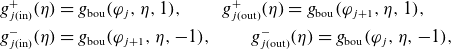 \begin{eqnarray} g^+_{j\text{(in)}}(\eta ) \;&=&\; g_{\text{bou}}(\varphi _j,\eta, 1), \qquad g^+_{j\text{(out)}}(\eta )=g_{\text{bou}}(\varphi _{j+1},\eta, 1), \nonumber \\ g^-_{j\text{(in)}}(\eta ) \;&=&\; g_{\text{bou}}(\varphi _{j+1},\eta, -1), \qquad g^-_{j\text{(out)}}(\eta )=g_{\text{bou}}(\varphi _j,\eta, -1), \end{eqnarray}
follows from (3.16) as
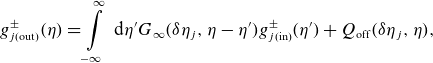 \begin{align} g^\pm _{j \text{(out)}}(\eta ) = \int \limits _{-\infty }^{\infty }\textrm { d}\eta ^\prime G_\infty (\delta \eta _j,\eta -\eta ^\prime ) g^\pm _{j \text{(in)}}(\eta ^\prime ) + Q_{\text{off}}(\delta \eta _j,\eta ), \end{align}
where
 \begin{align} \delta \eta _j=\delta \eta (\varphi _j,\varphi _{j+1})=\left (2\eta _b I_j(\eta _b)\right )^{1/2}l_c^{-1/2}, \qquad Q_{\text{off}}(\delta \eta _j,\eta ) = Q_\sigma (\varphi _j,\varphi _{j+1},\eta ), \end{align}
and $I_j(\eta )$
is given by (2.26) so that
$I_j(\eta )$
is given by (2.26) so that $\delta \eta _j = \pi ^{1/2}\delta \eta _e$
, see (3.9). Conditions (3.14) with
$\delta \eta _j = \pi ^{1/2}\delta \eta _e$
, see (3.9). Conditions (3.14) with $\delta \varphi \rightarrow 0$
link the incoming distributions
$\delta \varphi \rightarrow 0$
link the incoming distributions $g^\pm _{j \text{(in)}}$
to the outgoing
$g^\pm _{j \text{(in)}}$
to the outgoing $g^\pm _{j \text{(out)}}$
as follows:
$g^\pm _{j \text{(out)}}$
as follows:
 \begin{eqnarray} g^+_{j \text{(in)}}(\eta \lt \eta _j) \;&=&\; g^+_{j-1 \text{(out)}}(\eta \lt \eta _j), \qquad g^+_{j \text{(in)}}(\eta \gt \eta _j)=g^-_{j \text{(out)}}(\eta \gt \eta _j), \\ g^-_{j \text{(in)}}(\eta \lt \eta _{j+1}) \;&=&\; g^+_{j+1 \text{(out)}}(\eta \lt \eta _{j+1}), \qquad g^-_{j \text{(in)}}(\eta \gt \eta _{j+1})=g^+_{j \text{(out)}}(\eta \gt \eta _{j+1}), \nonumber \end{eqnarray}
where $\eta _j = 1/B(\varphi _j)$
. Substitution of
$\eta _j = 1/B(\varphi _j)$
. Substitution of $g_{j\text{(in)}}^\pm$
into the mapping (3.25) via (3.27) leads to a coupled set of Wiener–Hopf-type integral equations for
$g_{j\text{(in)}}^\pm$
into the mapping (3.25) via (3.27) leads to a coupled set of Wiener–Hopf-type integral equations for $g_{j\text{(out)}}^\pm$
. Introducing a dimensionless variable
$g_{j\text{(out)}}^\pm$
. Introducing a dimensionless variable $x$
and dimensionless distribution function
$x$
and dimensionless distribution function $\alpha _j^\pm$
as follows:
$\alpha _j^\pm$
as follows:
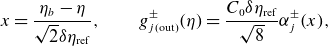 \begin{align} x=\frac {\eta _b-\eta }{\sqrt {2}\delta \eta _{\textrm {ref}}}, \qquad g_{j\text{(out)}}^\pm (\eta )=\frac {C_0 \delta \eta _{\textrm{ref}}}{\sqrt {8}}\alpha _j^\pm (x), \end{align}
where $\delta \eta _{\textrm {ref}}$
is some reference boundary layer width which is set in case of a closed field line to the largest
$\delta \eta _{\textrm {ref}}$
is some reference boundary layer width which is set in case of a closed field line to the largest $\delta \eta _j$
, this set is of the form
$\delta \eta _j$
, this set is of the form
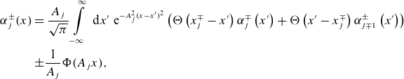 \begin{eqnarray} \alpha _j^\pm (x) \;&=&\; \frac {A_j}{\sqrt {\pi }}\int \limits _{-\infty }^\infty \textrm { d} x^\prime \textrm { e}^{-A_j^2(x-x^\prime )^2} \left ( \Theta \left (x^\mp _j-x^\prime \right )\alpha _j^\mp \left (x^\prime \right ) + \Theta \left (x^\prime -x^\mp _j\right )\alpha _{j\mp 1}^\pm \left (x^\prime \right ) \right ) \nonumber \\ &\pm & \frac {1}{A_j}\Phi (A_j x), \end{eqnarray}
where mis-alignments of relevant maxima $x_j^\pm \lt 0$
and aspect ratios
$x_j^\pm \lt 0$
and aspect ratios $A_j$
are
$A_j$
are
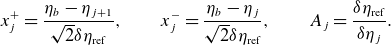 \begin{align} x_j^+=\frac {\eta _b -\eta _{j+1}}{\sqrt {2}\delta \eta _{\text{ref}}}, \qquad x_j^-=\frac {\eta _b -\eta _j}{\sqrt {2}\delta \eta _{\text{ref}}}, \qquad A_j=\frac {\delta \eta _{\text{ref}}}{\delta \eta _j}. \end{align}
It should be noted that solution of set (3.29) is determined up to the null space of the original operator $\hat L$
, (2.3), which is an arbitrary constant, i.e.
$\hat L$
, (2.3), which is an arbitrary constant, i.e. $\alpha ^\pm _j=\text {const}$
, and which produces no particle flux or parallel current but only re-defines the equilibrium Maxwellian.
$\alpha ^\pm _j=\text {const}$
, and which produces no particle flux or parallel current but only re-defines the equilibrium Maxwellian.
3.3. Alignment of maxima, equivalent ripples
An obvious consequence of (3.29) is the configuration where the leading-order off-set is absent. Namely, coupled set (3.29) reduces to two coupled equations in the case that all trapping domains are equivalent, which means that all relevant maxima are aligned with a global maximum, $x_j^\pm =0$
, and all aspect ratios are the same (equal to one),
$x_j^\pm =0$
, and all aspect ratios are the same (equal to one), $A_j=1$
. The first condition means that global maximum is reached on a line (lines) rather than at a point (points). The second condition means that all
$A_j=1$
. The first condition means that global maximum is reached on a line (lines) rather than at a point (points). The second condition means that all $\delta \eta _j$
are the same, i.e. the integral (3.20) between maximum points is the same for all trapping domains. In other words, this means that the value of the first integral (2.26) at the trapped–passing boundary
$\delta \eta _j$
are the same, i.e. the integral (3.20) between maximum points is the same for all trapping domains. In other words, this means that the value of the first integral (2.26) at the trapped–passing boundary $\eta =\eta _b$
does not depend on field line parameter
$\eta =\eta _b$
does not depend on field line parameter $\vartheta _0$
,
$\vartheta _0$
,
 \begin{align} \frac {\partial I_j(\vartheta _0,\eta _b)}{\partial \vartheta _0} = 0, \qquad I_j(\vartheta _0,\eta )= \frac {1}{2}\oint \frac {\textrm { d} l}{B} \lambda =\frac {1}{2v}\oint \frac {\textrm { d} l}{B} v_\parallel . \end{align}
Thus, $\alpha ^\pm _j(x)=\alpha ^\pm$
, and the set (3.29), respectively, closes to the form
$\alpha ^\pm _j(x)=\alpha ^\pm$
, and the set (3.29), respectively, closes to the form
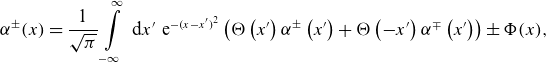 \begin{align} \alpha ^\pm (x) = \frac {1}{\sqrt {\pi }}\int \limits _{-\infty }^\infty \textrm { d} x^\prime \textrm { e}^{-(x-x^\prime )^2} \left ( \Theta \left (x^\prime \right )\alpha ^\pm \left (x^\prime \right ) + \Theta \left ({-}x^\prime \right )\alpha ^\mp \left (x^\prime \right ) \right ) \pm \Phi (x), \end{align}
corresponding to quasi-symmetry (Nührenberg & Zille, Reference Nührenberg and Zille1988) (omnigeneity (Cary & Shasharina Reference Cary and Shasharina1997; Helander & Nührenberg, Reference Helander and Nührenberg2009)). Obviously, the even part of the solution $\alpha ^++\alpha ^-$
satisfies a homogeneous equation and thus is constant, which we set to zero. Expressing
$\alpha ^++\alpha ^-$
satisfies a homogeneous equation and thus is constant, which we set to zero. Expressing $\alpha ^-=-\alpha ^+$
, set (3.32) is reduced to a single Wiener–Hopf-type integral equation
$\alpha ^-=-\alpha ^+$
, set (3.32) is reduced to a single Wiener–Hopf-type integral equation
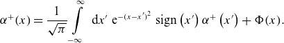 \begin{align} \alpha ^+(x) = \frac {1}{\sqrt {\pi }}\int \limits _{-\infty }^\infty \textrm { d} x^\prime \textrm { e}^{-(x-x^\prime )^2} \textrm { sign}\left (x^\prime \right )\alpha ^+\left (x^\prime \right ) +\Phi (x). \end{align}
Obviously, deep in the trapped region $x\rightarrow -\infty$
where
$x\rightarrow -\infty$
where $\Phi (x)\rightarrow 0$
and
$\Phi (x)\rightarrow 0$
and $\alpha ^+ \rightarrow \text{const}$
, this equation reduces to
$\alpha ^+ \rightarrow \text{const}$
, this equation reduces to $\alpha ^+=-\alpha ^+$
, i.e. it results in zero off-set
$\alpha ^+=-\alpha ^+$
, i.e. it results in zero off-set $\alpha ^\pm =0$
. Actually, as shown in (Helander et al. Reference Helander, Geiger and Maassberg2011), the ripple equivalence condition (3.31), which is fulfilled for a perfectly quasi-isodynamic stellarator where the magnetic field is omnigeneous, allows reduction of the boundary layer problem to a tokamak-like problem up to the same degree of accuracy as the analysis here (essentially, we use the integral representation of the same problem as in Helander et al. Reference Helander, Geiger and Maassberg2011).
$\alpha ^\pm =0$
. Actually, as shown in (Helander et al. Reference Helander, Geiger and Maassberg2011), the ripple equivalence condition (3.31), which is fulfilled for a perfectly quasi-isodynamic stellarator where the magnetic field is omnigeneous, allows reduction of the boundary layer problem to a tokamak-like problem up to the same degree of accuracy as the analysis here (essentially, we use the integral representation of the same problem as in Helander et al. Reference Helander, Geiger and Maassberg2011).
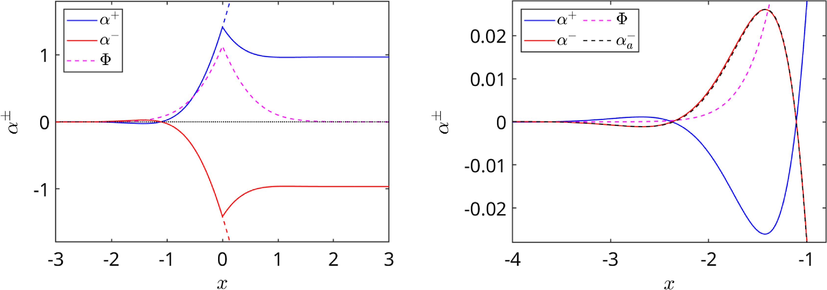
Figure 12. Normalized distribution functions $\alpha ^+$
(blue),
$\alpha ^+$
(blue), $\alpha ^-$
(red) and source function
$\alpha ^-$
(red) and source function $\Phi$
(magenta). Full normalized distribution functions,
$\Phi$
(magenta). Full normalized distribution functions, $\alpha ^{\pm }+\alpha _{1/\nu }^\pm$
, are shown with dashed lines. The right picture is a zoom to the trapped region, where also the asymptotic solution (3.34) is shown (black dashed).
$\alpha ^{\pm }+\alpha _{1/\nu }^\pm$
, are shown with dashed lines. The right picture is a zoom to the trapped region, where also the asymptotic solution (3.34) is shown (black dashed).
Solutions to the equation set (3.32) are shown in figure 12 together with asymptotic solution (3.8) expressed in terms of normalized variables using $\delta \eta _j=\delta \eta _{\text{ref}}=\sqrt {\pi }\delta \eta _e$
as
$\delta \eta _j=\delta \eta _{\text{ref}}=\sqrt {\pi }\delta \eta _e$
as
 \begin{align} \alpha ^\pm _{a}(x)=\pm \alpha _0 \exp \left (\sqrt {2\pi }\; x \right )\cos \left (\sqrt {2\pi }\; x +\phi \right ), \end{align}
where $\alpha _0=\text {const}$
. They agree well because the latter solution must actually be the same as
$\alpha _0=\text {const}$
. They agree well because the latter solution must actually be the same as $\alpha ^\pm$
in the region where the source term is negligible. We can recover the full solution if we add to
$\alpha ^\pm$
in the region where the source term is negligible. We can recover the full solution if we add to $\alpha ^\pm (x)$
the rescaled leading-order term (2.46) expanded to the linear order in
$\alpha ^\pm (x)$
the rescaled leading-order term (2.46) expanded to the linear order in $\eta -\eta _b$
,
$\eta -\eta _b$
,
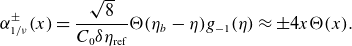 \begin{align} \alpha ^\pm _{1/\nu }(x)=\frac {\sqrt {8}}{C_0 \delta \eta _{\text{ref}}}\Theta (\eta _b-\eta )g_{-1}(\eta )\approx \pm 4 x \Theta (x). \end{align}
Naturally, full solution $\alpha ^\pm (x)+\alpha ^\pm _{1/\nu }(x)$
has a continuous derivative at the trapped–passing boundary.
$\alpha ^\pm (x)+\alpha ^\pm _{1/\nu }(x)$
has a continuous derivative at the trapped–passing boundary.
Note that alignment of maxima, $x_j^\pm =0$
, is not sufficient on its own, without conditions of equal aspect ratios,
$x_j^\pm =0$
, is not sufficient on its own, without conditions of equal aspect ratios, $A_j=1$
, for avoiding the leading-order off-set. This can be seen from figure 13, where a solution to (3.29) is shown for the case of three relevant trapping domains and aligned maxima but different aspect ratios,
$A_j=1$
, for avoiding the leading-order off-set. This can be seen from figure 13, where a solution to (3.29) is shown for the case of three relevant trapping domains and aligned maxima but different aspect ratios, $A_0=A_2=2$
and
$A_0=A_2=2$
and $A_1=1$
(i.e.
$A_1=1$
(i.e. $2\delta \eta _0=2\delta \eta _2=\delta \eta _1 \equiv \delta \eta _{\text{ref}}$
). A finite off-set in the first and last domains,
$2\delta \eta _0=2\delta \eta _2=\delta \eta _1 \equiv \delta \eta _{\text{ref}}$
). A finite off-set in the first and last domains, $\alpha _2^\pm ({-}\infty )= - \alpha _0^\pm ({-}\infty )$
, can be clearly seen. In such a case, the function
$\alpha _2^\pm ({-}\infty )= - \alpha _0^\pm ({-}\infty )$
, can be clearly seen. In such a case, the function $g_{\text{bou}}$
in the trapped particle domain and, respectively, bootstrap coefficient, diverge at low collisionality as
$g_{\text{bou}}$
in the trapped particle domain and, respectively, bootstrap coefficient, diverge at low collisionality as $\lambda _{bB} \sim \nu ^{-1/2}$
(see the normalization (3.18) and (3.28)).
$\lambda _{bB} \sim \nu ^{-1/2}$
(see the normalization (3.18) and (3.28)).
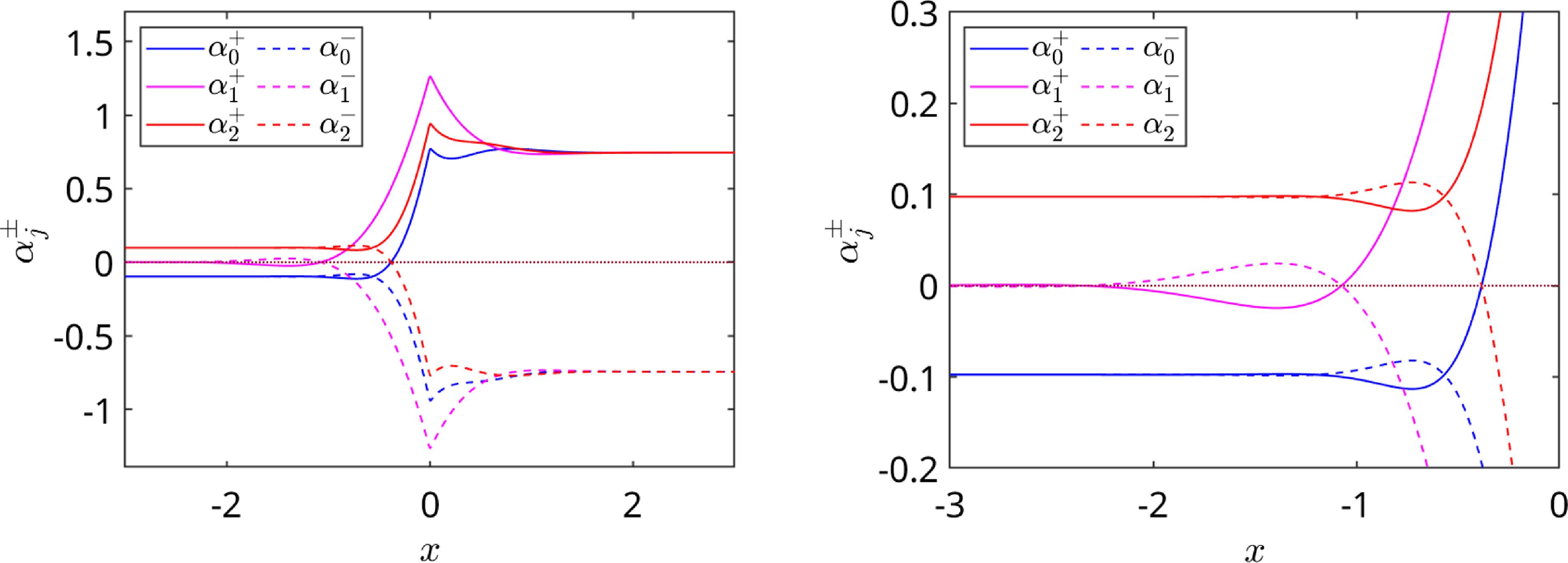
Figure 13. Normalized distribution functions $\alpha _j^+$
(solid) and
$\alpha _j^+$
(solid) and $\alpha _j^-$
(dashed) in the case of three relevant trapping domains per closed field line. The right picture is a zoom to the trapped particle domain.
$\alpha _j^-$
(dashed) in the case of three relevant trapping domains per closed field line. The right picture is a zoom to the trapped particle domain.
A particular example of configurations where the bootstrap coefficient diverges in the $1/\nu$
regime in this way is a family of ‘anti-sigma optimized’ configurations, i.e. configurations where sigma optimization (Mynick et al. Reference Mynick, Chu and Boozer1982; Shaing & Hokin Reference Shaing and Hokin1983) is applied to align maxima instead of minima. A magnetic field strength for a particular family of such configurations with dominant toroidal ripple is of the form
$1/\nu$
regime in this way is a family of ‘anti-sigma optimized’ configurations, i.e. configurations where sigma optimization (Mynick et al. Reference Mynick, Chu and Boozer1982; Shaing & Hokin Reference Shaing and Hokin1983) is applied to align maxima instead of minima. A magnetic field strength for a particular family of such configurations with dominant toroidal ripple is of the form
 \begin{align} B(\vartheta, \varphi )=B_0\left (1+\varepsilon _0 \cos \left (N_{\text{tor}}\varphi \right ) + f(\vartheta )\left (1-\cos \left (N_{\text{tor}}\varphi \right )\right )\right ), \end{align}
where $B_0$
and
$B_0$
and $\varepsilon _0$
are constant parameters,
$\varepsilon _0$
are constant parameters, $N_{\text{tor}}$
is the number of field periods and
$N_{\text{tor}}$
is the number of field periods and $f(\vartheta )\lt \varepsilon _0$
. For the computations with NEO-2, we use the following simple form of this function:
$f(\vartheta )\lt \varepsilon _0$
. For the computations with NEO-2, we use the following simple form of this function:
 \begin{align} f(\vartheta )=\varepsilon _1 \cos \vartheta + \varepsilon _3\cos (3\vartheta ), \end{align}
with $\varepsilon _0=0.125$
,
$\varepsilon _0=0.125$
, $\varepsilon _1=0.05$
and two values of
$\varepsilon _1=0.05$
and two values of $\varepsilon _3$
. We set
$\varepsilon _3$
. We set $N_{\text{tor}}=1$
and
$N_{\text{tor}}=1$
and $\iota =1/4$
to get 4 relevant domains (ripples) on a closed field line passing through the point
$\iota =1/4$
to get 4 relevant domains (ripples) on a closed field line passing through the point $(\vartheta, \varphi )=(0,0)$
. In the case
$(\vartheta, \varphi )=(0,0)$
. In the case $\varepsilon _3=0$
(case 1), condition
$\varepsilon _3=0$
(case 1), condition $A_j=1$
does not hold, and a strong off-set of the bootstrap coefficient
$A_j=1$
does not hold, and a strong off-set of the bootstrap coefficient $\lambda _{bB} \propto \nu ^{-1/2}$
is seen in figure 14. In the case
$\lambda _{bB} \propto \nu ^{-1/2}$
is seen in figure 14. In the case $\varepsilon _3=0.06994425$
(case 2) all four ripples are equivalent,
$\varepsilon _3=0.06994425$
(case 2) all four ripples are equivalent, $A_j=1$
, and the leading-order off-set is absent. However, there still remains a residual off-set driven by source
$A_j=1$
, and the leading-order off-set is absent. However, there still remains a residual off-set driven by source $\Delta s$
, (3.13), which includes constant and logarithmic parts,
$\Delta s$
, (3.13), which includes constant and logarithmic parts, $\delta \lambda _{bB} \rightarrow C_1+C_2 \log (\nu _\ast )$
, see the previous section. It should be noted that
$\delta \lambda _{bB} \rightarrow C_1+C_2 \log (\nu _\ast )$
, see the previous section. It should be noted that $\nu ^{-1/2}$
divergence of
$\nu ^{-1/2}$
divergence of $\lambda _{bB}$
in the case of aligned maxima but non-equivalent ripples is not a property of a closed field line. A similar behavior is seen also for the case
$\lambda _{bB}$
in the case of aligned maxima but non-equivalent ripples is not a property of a closed field line. A similar behavior is seen also for the case $\varepsilon _3=0$
at the irrational flux surface with
$\varepsilon _3=0$
at the irrational flux surface with $\iota =(1+\sqrt {5})/20 \approx 0.1618$
labeled there as case 3.
$\iota =(1+\sqrt {5})/20 \approx 0.1618$
labeled there as case 3.
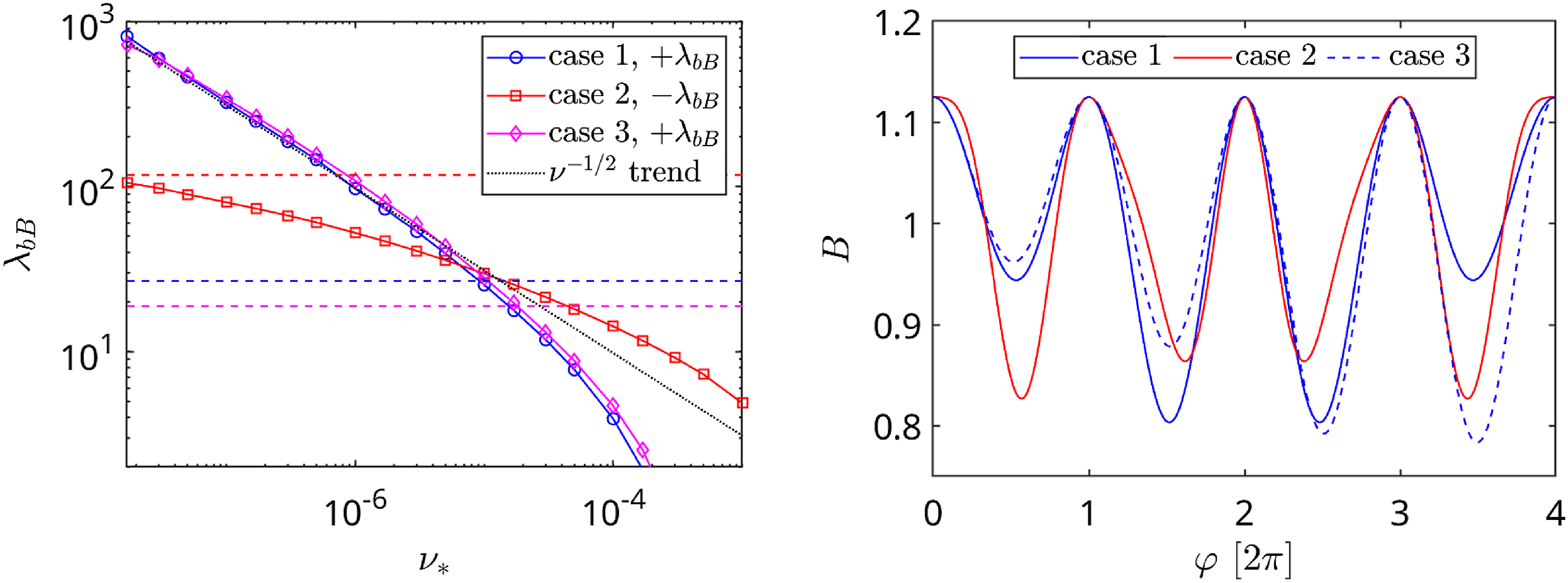
Figure 14. Left: normalized bootstrap coefficient $\lambda _{bB}$
, (2.44), computed by NEO-2 for “anti-sigma optimized” configurations in cases 1, 2 and 3 (see the legend) as function of normalized collisionality
$\lambda _{bB}$
, (2.44), computed by NEO-2 for “anti-sigma optimized” configurations in cases 1, 2 and 3 (see the legend) as function of normalized collisionality $\nu _\ast$
. For each case, the Shaing–Callen limit (2.43) is shown with a dashed line of the respective color. Sign of
$\nu _\ast$
. For each case, the Shaing–Callen limit (2.43) is shown with a dashed line of the respective color. Sign of $\lambda _{bB}$
(but not of the respective asymptotic) is reversed in case 2. Right: magnetic field strength
$\lambda _{bB}$
(but not of the respective asymptotic) is reversed in case 2. Right: magnetic field strength $B(\varphi )$
, (3.36) for these cases plotted along the field line within the first four toroidal periods.
$B(\varphi )$
, (3.36) for these cases plotted along the field line within the first four toroidal periods.
3.4. Non-aligned maxima, large aspect ratio
Let us consider now a more typical situation where local field maxima are not aligned. For simplicity, we consider a configuration with short ripples located near a global maximum adjacent to a long ripple, as in the case of the first rippled tokamak configuration (2.57) with $\iota =1/4$
illustrated in figures 3 and 6. Besides the global maximum, there are only two relevant maxima at low collisionalities. They separate two short and shallow trapping domains, called below ‘off-set domains’, from a wide domain in between, called below the ‘main region’. Setting
$\iota =1/4$
illustrated in figures 3 and 6. Besides the global maximum, there are only two relevant maxima at low collisionalities. They separate two short and shallow trapping domains, called below ‘off-set domains’, from a wide domain in between, called below the ‘main region’. Setting $\delta \eta _{\text{ref}}=\delta \eta _1$
so that
$\delta \eta _{\text{ref}}=\delta \eta _1$
so that $A_1=1$
, aspect ratios for off-set domains are the same,
$A_1=1$
, aspect ratios for off-set domains are the same, $A_0=A_2\equiv A_o$
. Respective value
$A_0=A_2\equiv A_o$
. Respective value $A_o \approx 23.7 \gg 1$
will be called below the ‘off-set aspect ratio’, or simply ‘aspect ratio’. To keep an example more general than the configuration with
$A_o \approx 23.7 \gg 1$
will be called below the ‘off-set aspect ratio’, or simply ‘aspect ratio’. To keep an example more general than the configuration with $\iota =1/4$
, we do not assume that the local maxima separating the main region from two off-set domains are the same (thus allowing broken stellarator symmetry). For the present example, it is convenient to change the general notation in (3.29) as follows,
$\iota =1/4$
, we do not assume that the local maxima separating the main region from two off-set domains are the same (thus allowing broken stellarator symmetry). For the present example, it is convenient to change the general notation in (3.29) as follows, $\alpha _0^\pm \equiv \alpha _{-o}^\pm$
,
$\alpha _0^\pm \equiv \alpha _{-o}^\pm$
, $\alpha _1^\pm \equiv \alpha ^\pm _{mr}$
and
$\alpha _1^\pm \equiv \alpha ^\pm _{mr}$
and $\alpha _2^\pm \equiv \alpha _{+o}^\pm$
, so that subscripts ‘
$\alpha _2^\pm \equiv \alpha _{+o}^\pm$
, so that subscripts ‘ $+o$
’ and ‘
$+o$
’ and ‘ $-o$
’ denote the left and right off-set domains, respectively, and subscript ‘
$-o$
’ denote the left and right off-set domains, respectively, and subscript ‘ $mr$
’ stands for the main region. Respective normalized mis-alignments of local maxima we re-notate as follows,
$mr$
’ stands for the main region. Respective normalized mis-alignments of local maxima we re-notate as follows, $x_1^+=x_2^- \equiv x_{-o}$
and
$x_1^+=x_2^- \equiv x_{-o}$
and $x_3^-=x_2^+ \equiv x_{+o}$
, see schematic figure 15. Thus, we cast the closed set of six equations (3.29) to
$x_3^-=x_2^+ \equiv x_{+o}$
, see schematic figure 15. Thus, we cast the closed set of six equations (3.29) to
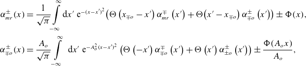 \begin{align*} \alpha _{mr}^\pm (x) &= \frac {1}{\sqrt {\pi }} \!\int \limits _{-\infty }^\infty \!\!\textrm { d} x^\prime \textrm { e}^{-(x-x^\prime )^2} \!\left ( \Theta \left (x_{\mp o}-x^\prime \right )\alpha _{mr}^\mp \left (x^\prime \right ) + \Theta \!\left (x^\prime -x_{\mp o}\right )\alpha _{\mp o}^\pm \left (x^\prime \right ) \right ) \pm \Phi (x), \nonumber \\ \alpha _{\mp o}^\pm (x) &= \frac {A_o}{\sqrt {\pi }}\int \limits _{-\infty }^\infty \textrm { d} x^\prime \textrm { e}^{-A_o^2(x-x^\prime )^2} \left ( \Theta \left ({-}x^\prime \right )\alpha _{\mp o}^\mp \left (x^\prime \right ) + \Theta \left (x^\prime \right )\alpha _{\pm o}^\pm \left (x^\prime \right ) \right ) \pm \frac {\Phi (A_o x)}{A_o}, \end{align*}
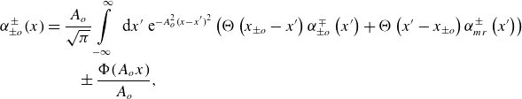 \begin{align} \alpha _{\pm o}^\pm (x) &= \frac {A_o}{\sqrt {\pi }}\int \limits _{-\infty }^\infty \textrm { d} x^\prime \textrm { e}^{-A_o^2(x-x^\prime )^2} \left ( \Theta \left (x_{\pm o}-x^\prime \right )\alpha _{\pm o}^\mp \left (x^\prime \right ) + \Theta \left (x^\prime -x_{\pm o}\right )\alpha _{mr}^\pm \left (x^\prime \right ) \right ) \nonumber\\ & \qquad\pm \frac {\Phi (A_o x)}{A_o}, \end{align}
where notation $\alpha _{\mp o}^\pm$
means that either
$\alpha _{\mp o}^\pm$
means that either $\alpha _{-o}^+$
or
$\alpha _{-o}^+$
or $\alpha _{+o}^-$
should be taken, and
$\alpha _{+o}^-$
should be taken, and $\alpha _{\pm o}^\pm$
means that either
$\alpha _{\pm o}^\pm$
means that either $\alpha _{+o}^+$
or
$\alpha _{+o}^+$
or $\alpha _{-o}^-$
should be taken.
$\alpha _{-o}^-$
should be taken.

Figure 15. Locations of normalized outgoing particle distributions $\alpha _{\pm o}^\pm$
and
$\alpha _{\pm o}^\pm$
and $\alpha _{mr}^\pm$
in the respective off-set domains and the main region. Positions of relevant maxima
$\alpha _{mr}^\pm$
in the respective off-set domains and the main region. Positions of relevant maxima $\varphi _j$
are shown with blue lines. Normalized misalignments
$\varphi _j$
are shown with blue lines. Normalized misalignments $x_{\pm o}$
are shown with red lines.
$x_{\pm o}$
are shown with red lines.
Due to $A_o \gg 1$
, source terms
$A_o \gg 1$
, source terms $\Phi (A_o x)/A_o$
can be ignored in the last two pairs of equations since
$\Phi (A_o x)/A_o$
can be ignored in the last two pairs of equations since $\alpha _{\mp o}^\pm \sim \alpha _{\pm o}^\pm \sim \alpha _{mr}^\pm \sim \Phi \gg \Phi /A_o$
. Since
$\alpha _{\mp o}^\pm \sim \alpha _{\pm o}^\pm \sim \alpha _{mr}^\pm \sim \Phi \gg \Phi /A_o$
. Since $\alpha ^\pm _{mr}(x)$
, which varies on the scale
$\alpha ^\pm _{mr}(x)$
, which varies on the scale $x\sim 1$
, changes little compared with the exponent in the sub-integrand of the last pair of equations, we can set there
$x\sim 1$
, changes little compared with the exponent in the sub-integrand of the last pair of equations, we can set there $\alpha ^\pm _{mr}\left (x^\prime \right ) \approx \alpha ^\pm _{mr}\left (x\right )$
. Thus, the last pair of (3.38) takes the approximate form
$\alpha ^\pm _{mr}\left (x^\prime \right ) \approx \alpha ^\pm _{mr}\left (x\right )$
. Thus, the last pair of (3.38) takes the approximate form
 \begin{align} \alpha _{\pm o}^\pm (x) \approx \frac {A_o}{\sqrt {\pi }}\int \limits _{-\infty }^{x_{\pm o}} \textrm { d} x^\prime \textrm { e}^{-A_o^2(x-x^\prime )^2} \alpha _{\pm o}^\mp \left (x^\prime \right ) + \tilde \Theta \left (A_o(x-x_{\pm o})\right ) \alpha _{mr}^\pm \left (x\right ), \end{align}
where we introduced a “smooth step” function as
 \begin{align} \tilde \Theta (x)\equiv \frac {1}{2} \left (1+\textrm { erf}(x) \right ), \qquad \lim \limits _{A_o\rightarrow \infty } \tilde \Theta (A_o x)=\Theta (x). \end{align}
Further analysis is strongly simplified if we restrict ourselves to the most probable case of strong mis-alignment of local maxima where boundary layers in both off-set domains associated with these maxima are well separated from the trapped–passing boundary, $\delta \eta _0 \ll |\eta _b-\eta _1|$
and
$\delta \eta _0 \ll |\eta _b-\eta _1|$
and $\delta \eta _2 \ll |\eta _b-\eta _2|$
. In normalized variables, these conditions mean
$\delta \eta _2 \ll |\eta _b-\eta _2|$
. In normalized variables, these conditions mean $A_o |x_{\pm o}| \gg 1$
. Since the first term in (3.39) is exponentially small in the region
$A_o |x_{\pm o}| \gg 1$
. Since the first term in (3.39) is exponentially small in the region $A_o (x-x_{\pm o}) \gg 1$
where also
$A_o (x-x_{\pm o}) \gg 1$
where also $\Theta \left (A_o(x-x_{\pm o})\right ) \approx 1$
, (3.39) results there in
$\Theta \left (A_o(x-x_{\pm o})\right ) \approx 1$
, (3.39) results there in $\alpha _{\pm o}^\pm (x) \approx \alpha _{mr}^\pm \left (x\right )$
. Thus, the second pair of (3.38) with the source term ignored approximately is
$\alpha _{\pm o}^\pm (x) \approx \alpha _{mr}^\pm \left (x\right )$
. Thus, the second pair of (3.38) with the source term ignored approximately is
 \begin{align} \alpha _{\mp o}^\pm (x) & \approx \frac {A_o}{\sqrt {\pi }}\int \limits _{-\infty }^\infty \textrm { d} x^\prime \textrm { e}^{-A_o^2(x-x^\prime )^2} \left ( \Theta \left ({-}x^\prime \right )\alpha _{mr}^\mp \left (x^\prime \right ) + \Theta \left (x^\prime \right )\alpha _{mr}^\pm \left (x^\prime \right ) \right ), \nonumber \\ & \qquad A_o (x-x_{\mp o}) \gg 1. \end{align}
Moreover, due to slow variation of $\alpha _{mr}^\pm (x^\prime )$
compared with the exponent, one can further simplify this expression to
$\alpha _{mr}^\pm (x^\prime )$
compared with the exponent, one can further simplify this expression to
 \begin{align} \alpha _{\mp o}^\pm (x) \approx \Theta \left ({-}x\right )\alpha _{mr}^\mp \left (x\right ) + \Theta \left (x\right )\alpha _{mr}^\pm \left (x\right ), \end{align}
which is valid in the region $x\gt x_{\mp o}$
except for small vicinities of class boundary,
$x\gt x_{\mp o}$
except for small vicinities of class boundary, $|x-x_{\mp o}| \leqslant 1/A_o$
, and trapped–passing boundary
$|x-x_{\mp o}| \leqslant 1/A_o$
, and trapped–passing boundary $|x| \leqslant 1/A_o$
, which contain local boundary layers of the off-set domains (layers of the width
$|x| \leqslant 1/A_o$
, which contain local boundary layers of the off-set domains (layers of the width $\delta \eta _0 \sim \delta \eta _2 \ll \delta \eta _1$
). Contribution of these vicinities to the integral in the first pair of (3.38) is of the order of
$\delta \eta _0 \sim \delta \eta _2 \ll \delta \eta _1$
). Contribution of these vicinities to the integral in the first pair of (3.38) is of the order of $1/A_o$
, and, therefore, this pair can be closed as follows:
$1/A_o$
, and, therefore, this pair can be closed as follows:
 \begin{align} \alpha _{mr}^\pm (x) = \frac {1}{\sqrt {\pi }}\int \limits _{-\infty }^\infty \textrm { d} x^\prime \textrm { e}^{-(x-x^\prime )^2} \left ( \Theta (x^\prime ) \alpha _{mr}^\pm \left (x^\prime \right ) + \Theta \left ({-}x^\prime \right )\alpha _{mr}^\mp \left (x^\prime \right ) \right ) \pm \Phi (x) + O(A_o^{-1}). \end{align}
Obviously, in the leading order over $A_o^{-1}$
, these equations are the same as (3.32) for equivalent ripples.
$A_o^{-1}$
, these equations are the same as (3.32) for equivalent ripples.
For the solution in local trapping regions of the off-set domains, $x \leqslant x_{\pm o}$
, Heaviside functions in the sub-integrands of the second pair of (3.38) can be replaced by their values at
$x \leqslant x_{\pm o}$
, Heaviside functions in the sub-integrands of the second pair of (3.38) can be replaced by their values at $x^\prime \lt 0$
which turns this pair (with the source term ignored) into
$x^\prime \lt 0$
which turns this pair (with the source term ignored) into
 \begin{align} \alpha _{\mp o}^\pm (x) = \frac {A_o}{\sqrt {\pi }}\int \limits _{-\infty }^\infty \textrm { d} x^\prime \textrm { e}^{-A_o^2(x-x^\prime )^2} \alpha _{\mp o}^\mp \left (x^\prime \right ). \end{align}
Substituting this result in (3.39), we note also that variation of the last term in (3.39) is determined in the region of interest by $\tilde \Theta$
while the factor
$\tilde \Theta$
while the factor $\alpha _{mr}^\pm$
varies slowly and can be replaced by its value at
$\alpha _{mr}^\pm$
varies slowly and can be replaced by its value at $x = x_{\pm o}$
. Introducing the new independent variable
$x = x_{\pm o}$
. Introducing the new independent variable $y=A_o(x-x_{\pm o})$
, equation set for
$y=A_o(x-x_{\pm o})$
, equation set for $\alpha ^\pm _{\pm o}$
reduces to two independent equations
$\alpha ^\pm _{\pm o}$
reduces to two independent equations
 \begin{align} \alpha _{\pm o}^\pm \left (x(y)\right ) \approx \frac {1}{\pi }\int \limits _{-\infty }^{0} \textrm { d} y^\prime \int \limits _{-\infty }^\infty \textrm { d} y^{\prime \prime } \textrm { e}^{-(y-y^\prime )^2-(y^\prime -y^{\prime \prime })^2} \alpha _{\pm o}^\pm \left (x(y^{\prime \prime })\right ) + \tilde \Theta \left (y\right ) \alpha _{mr}^\pm \left (x_{\pm o}\right ), \end{align}
which have constant solutions
 \begin{align} \alpha _{\pm o}^\pm \left (x(y)\right ) = \alpha _{mr}^\pm \left (x_{\pm o}\right ), \qquad \alpha ^\mp _{\pm o}=\alpha ^\pm _{\pm o}. \end{align}
Thus, we obtained an intuitively clear result that
-
• The distribution function in the main region (long ripple) is weakly affected by off-set domains (short ripples) which provide only a correction of the order of $A_o^{-1}$
.
$A_o^{-1}$
. -
• The distribution function in the off-set well takes the value of the distribution function in the main region at the local minimum point
$(\varphi _j,\eta _j)$
separating the main region and the off-set domain (see also figure 6).


The last conclusion can be easily generalized to the case where a short off-set domain is separated from two long main regions by local maxima on both sides. Assuming that solutions in both main regions are known, the off-set is determined by the solution in the main region separated from the off-set domain by the lower local maximum (this local maximum determines the class-transition boundary $\eta _c$
limiting the region
$\eta _c$
limiting the region $\eta \gt \eta _c$
with particles trapped in the off-set domain).
$\eta \gt \eta _c$
with particles trapped in the off-set domain).
The large aspect ratio approximation, $A_o=23.7$
, is checked in figure 16, where the left picture corresponds to the stellarator-symmetric case of figure 6 and in the right picture symmetry of local maxima is destroyed by setting
$A_o=23.7$
, is checked in figure 16, where the left picture corresponds to the stellarator-symmetric case of figure 6 and in the right picture symmetry of local maxima is destroyed by setting $x_{-o}=2 x_{+o}$
. It can be seen that approximation (3.46) is good in its validity domain and is violated for small mis-match parameter values
$x_{-o}=2 x_{+o}$
. It can be seen that approximation (3.46) is good in its validity domain and is violated for small mis-match parameter values $x_{\pm o} \leqslant A_o^{-1}$
. The finite off-set value for aligned maxima,
$x_{\pm o} \leqslant A_o^{-1}$
. The finite off-set value for aligned maxima, $x_{\pm o}=0$
, is the result of
$x_{\pm o}=0$
, is the result of $A_o \ne 1$
. Note that left figure 16 corresponds to collisionality dependence of the off-sets in case of fixed magnetic field geometry. This dependence for the first local ripple is shown for the dimensional distribution function (3.28) in figure 17 where it is compared with the NEO-2 result. Since
$A_o \ne 1$
. Note that left figure 16 corresponds to collisionality dependence of the off-sets in case of fixed magnetic field geometry. This dependence for the first local ripple is shown for the dimensional distribution function (3.28) in figure 17 where it is compared with the NEO-2 result. Since $g_{\text{bou}}$
is given there by propagator method in the leading order only, we added error bars to the result of (3.29) showing the order of magnitude estimate of the omitted correction term
$g_{\text{bou}}$
is given there by propagator method in the leading order only, we added error bars to the result of (3.29) showing the order of magnitude estimate of the omitted correction term $\Delta g_{\text{bou}}$
driven by the source
$\Delta g_{\text{bou}}$
driven by the source $\Delta s$
in (3.11). According to (3.12), this correction term is driven by the sources in the passing particle region and is of the order of
$\Delta s$
in (3.11). According to (3.12), this correction term is driven by the sources in the passing particle region and is of the order of $g_0^t$
at the trapped–passing boundary (and in the whole boundary layer) because
$g_0^t$
at the trapped–passing boundary (and in the whole boundary layer) because $\Delta g_{\text{bou}}$
must restore periodicity in the passing region. Since there are no sources in the trapped particle region,
$\Delta g_{\text{bou}}$
must restore periodicity in the passing region. Since there are no sources in the trapped particle region, $\Delta g_{\text{bou}}$
decays exponentially outside the boundary layer, as follows from (3.8) and from the solution
$\Delta g_{\text{bou}}$
decays exponentially outside the boundary layer, as follows from (3.8) and from the solution $\alpha ^+(x)$
for equivalent ripples, (3.33), where
$\alpha ^+(x)$
for equivalent ripples, (3.33), where $x$
is defined in (3.28). Therefore, we extend the estimate of the correction term to the whole trapped particle region by using
$x$
is defined in (3.28). Therefore, we extend the estimate of the correction term to the whole trapped particle region by using $\Delta g_{\text{bou}} \sim g_0^t \alpha ^+ (x)$
. This simple estimation gives an error bar
$\Delta g_{\text{bou}} \sim g_0^t \alpha ^+ (x)$
. This simple estimation gives an error bar $g_0^t \alpha ^+ (x_{\pm o})$
that decreases when
$g_0^t \alpha ^+ (x_{\pm o})$
that decreases when $x_{\pm o} \propto \nu _\ast ^{-1/2}$
increases.
$x_{\pm o} \propto \nu _\ast ^{-1/2}$
increases.


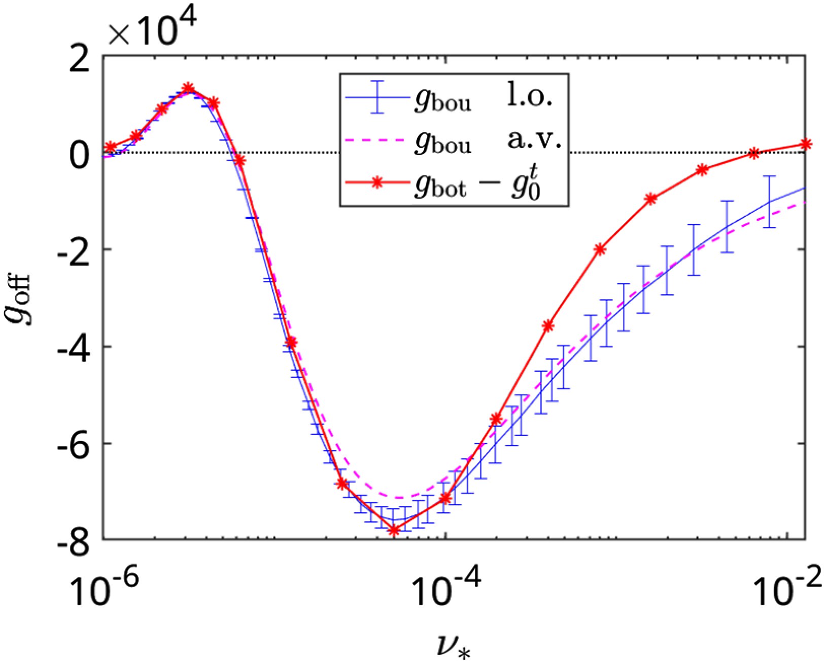
Figure 17. Distribution function off-set $g_{\text {off}} = g_{(3)} - g_0^t$
at the bottom of the first local well,
$g_{\text {off}} = g_{(3)} - g_0^t$
at the bottom of the first local well, $j=0$
, as a function of collisionality parameter
$j=0$
, as a function of collisionality parameter $\nu _\ast$
for configuration in figure 7. Blue – leading-order solution for
$\nu _\ast$
for configuration in figure 7. Blue – leading-order solution for $g_{\text{bou}}$
via (3.29), magenta – its large aspect ratio approximation (3.46), red – off-set
$g_{\text{bou}}$
via (3.29), magenta – its large aspect ratio approximation (3.46), red – off-set $g_{\text{off}}=g_{\text{bot}}-g_0^t$
via the result of NEO-2 shown in figure 7.
$g_{\text{off}}=g_{\text{bot}}-g_0^t$
via the result of NEO-2 shown in figure 7.
3.5. Weakly non-equivalent ripples
An important case is that of weakly non-equivalent ripples where the conditions of alignment of local maxima, $\eta _j=\eta _b$
, and of equal aspect ratios,
$\eta _j=\eta _b$
, and of equal aspect ratios, $A_j=1$
, are only slightly violated. Assuming infinitesimal mis-alignments
$A_j=1$
, are only slightly violated. Assuming infinitesimal mis-alignments $\eta _j-\eta _b$
and aspect ratio perturbations
$\eta _j-\eta _b$
and aspect ratio perturbations $\Delta A_j = A_j-1$
and looking for the solution of (3.29) in the form
$\Delta A_j = A_j-1$
and looking for the solution of (3.29) in the form $\alpha ^\pm _j = \alpha ^\pm +\Delta \alpha ^\pm _j$
, where
$\alpha ^\pm _j = \alpha ^\pm +\Delta \alpha ^\pm _j$
, where $\alpha ^+=-\alpha ^-$
are the solution to (quasi-symmetric) (3.32), the equation for the linear-order correction
$\alpha ^+=-\alpha ^-$
are the solution to (quasi-symmetric) (3.32), the equation for the linear-order correction $\Delta \alpha ^\pm _j$
is
$\Delta \alpha ^\pm _j$
is
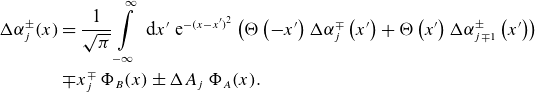 \begin{eqnarray} \Delta \alpha _j^\pm (x) \;&=&\; \frac {1}{\sqrt {\pi }} \int \limits _{-\infty }^\infty \textrm { d} x^\prime \textrm { e}^{-(x-x^\prime )^2} \left ( \Theta \left ({-}x^\prime \right )\Delta \alpha _j^\mp \left (x^\prime \right ) + \Theta \left (x^\prime \right )\Delta \alpha _{j\mp 1}^\pm \left (x^\prime \right ) \right ) \nonumber \\ &\mp & x^\mp _j\; \Phi _B(x) \pm \Delta A_j\; \Phi _A(x). \end{eqnarray}
Here, the first source term is due to small mis-alignment of maxima $|x^\mp _j| \ll 1$
with
$|x^\mp _j| \ll 1$
with
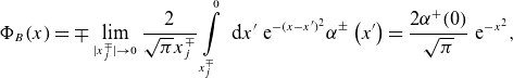 \begin{eqnarray} \Phi _B(x) = \mp \lim _{|x^\mp _j| \rightarrow 0}\frac {2}{\sqrt {\pi }x^\mp _j} \int \limits _{x^\mp _j}^0 \textrm { d} x^\prime \textrm { e}^{-(x-x^\prime )^2} \alpha ^\pm \left (x^\prime \right ) = \frac {2 \alpha ^+(0)}{\sqrt {\pi }} \textrm { e}^{-x^2}, \end{eqnarray}
and the second source term is due to small differences in boundary layer widths $|\Delta A_j| \ll 1$
with
$|\Delta A_j| \ll 1$
with
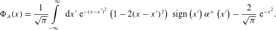 \begin{align} \Phi _A(x) = \frac {1}{\sqrt {\pi }}\int \limits _{-\infty }^\infty \textrm { d} x^\prime \textrm { e}^{-(x-x^\prime )^2} \left (1-2 (x-x^\prime )^2\right ) \textrm { sign}\left (x^\prime \right ) \alpha ^+\left (x^\prime \right ) -\frac {2}{\sqrt {\pi }}\textrm { e}^{-x^2}. \end{align}
Let us assume now an infinite number of ripples, $-\infty \lt j \lt \infty$
, with only the first maximum mis-aligned,
$-\infty \lt j \lt \infty$
, with only the first maximum mis-aligned, $\eta _1-\eta _b=\Delta \eta \ne 0$
, while the rest are aligned perfectly. Then the non-zero normalized mis-alignments are
$\eta _1-\eta _b=\Delta \eta \ne 0$
, while the rest are aligned perfectly. Then the non-zero normalized mis-alignments are $x_0^+=x_1^-=-\Delta x \equiv - \Delta \eta /(\sqrt {2}\delta \eta _{\text{ref}})$
and the rest
$x_0^+=x_1^-=-\Delta x \equiv - \Delta \eta /(\sqrt {2}\delta \eta _{\text{ref}})$
and the rest $x_j^\pm =0$
. In the absence of
$x_j^\pm =0$
. In the absence of $\Delta A_j=0$
, solution to (3.47) is anti-symmetric with respect to the mis-aligned maximum,
$\Delta A_j=0$
, solution to (3.47) is anti-symmetric with respect to the mis-aligned maximum, $\Delta \alpha _0^\pm = - \Delta \alpha _1^\mp$
,
$\Delta \alpha _0^\pm = - \Delta \alpha _1^\mp$
, $\Delta \alpha _{-1}^\pm = - \Delta \alpha _2^\mp$
, etc. Thus, ripples
$\Delta \alpha _{-1}^\pm = - \Delta \alpha _2^\mp$
, etc. Thus, ripples $j \leqslant 0$
are eliminated from the set (3.47), where the only inhomogeneous equation is
$j \leqslant 0$
are eliminated from the set (3.47), where the only inhomogeneous equation is
 \begin{align} \Delta \alpha _1^+(x) = \frac {1}{\sqrt {\pi }} \int \limits _{-\infty }^\infty \textrm { d} x^\prime \textrm { e}^{-(x-x^\prime )^2} \left ( \Theta \left ({-}x^\prime \right )\Delta \alpha _1^-\left (x^\prime \right ) - \Theta \left (x^\prime \right )\Delta \alpha _{1}^+\left (x^\prime \right ) \right )+\Delta x\; \Phi _B(x), \end{align}
while equations for $\Delta \alpha ^-_1$
and
$\Delta \alpha ^-_1$
and $\Delta \alpha _j^\pm$
with
$\Delta \alpha _j^\pm$
with $j\gt 1$
are given by the homogeneous set (3.47) with
$j\gt 1$
are given by the homogeneous set (3.47) with $x_j^\pm =\Delta A_j=0$
.
$x_j^\pm =\Delta A_j=0$
.
In the other case of perfectly aligned maxima, $x_j^\pm =0$
, and only one perturbed aspect ratio,
$x_j^\pm =0$
, and only one perturbed aspect ratio, $\Delta A_0 \ne 0$
and
$\Delta A_0 \ne 0$
and $\Delta A_j=0$
for
$\Delta A_j=0$
for $j \ne 0$
, solutions are anti-symmetric with respect to ripple
$j \ne 0$
, solutions are anti-symmetric with respect to ripple $j=0$
, i.e.
$j=0$
, i.e. $\Delta \alpha _{-j}^\pm = - \Delta \alpha _j^\mp$
. Thus, solutions with
$\Delta \alpha _{-j}^\pm = - \Delta \alpha _j^\mp$
. Thus, solutions with $j\lt 0$
are again eliminated from the set where the only inhomogeneous equation is
$j\lt 0$
are again eliminated from the set where the only inhomogeneous equation is
 \begin{align} \Delta \alpha _0^+(x) & = -\frac {1}{\sqrt {\pi }} \int \limits _{-\infty }^\infty \textrm { d} x^\prime \textrm { e}^{-(x-x^\prime )^2} \left ( \Theta \left ({-}x^\prime \right )\Delta \alpha _0^+\left (x^\prime \right ) + \Theta \left (x^\prime \right )\Delta \alpha _{1}^-\left (x^\prime \right ) \right ) \nonumber \\ & + \Delta A_0\; \Phi _A(x), \end{align}
while the rest $\Delta \alpha _j^\pm$
are given by the homogeneous set (3.47) for
$\Delta \alpha _j^\pm$
are given by the homogeneous set (3.47) for $j\gt 0$
.
$j\gt 0$
.
Off-set factors $\Delta _j^{A,B}=\Delta \alpha _j^+({-}\infty )=\Delta \alpha _j^-({-}\infty )$
as functions of ripple index
$\Delta _j^{A,B}=\Delta \alpha _j^+({-}\infty )=\Delta \alpha _j^-({-}\infty )$
as functions of ripple index $j$
are shown in figure 18. Factors
$j$
are shown in figure 18. Factors $\Delta _j^B$
are due to mis-alignment of a single local maximum between ripples 0 and 1 (
$\Delta _j^B$
are due to mis-alignment of a single local maximum between ripples 0 and 1 ( $\Delta x =1$
and
$\Delta x =1$
and $\Delta A_0=0$
) and
$\Delta A_0=0$
) and $\Delta _j^A$
are due to violation of the aspect ratio in ripple 0 (
$\Delta _j^A$
are due to violation of the aspect ratio in ripple 0 ( $\Delta x =0$
and
$\Delta x =0$
and $\Delta A_0=1$
). Off-set
$\Delta A_0=1$
). Off-set $\Delta ^B_j$
is mainly produced in ripples 0 and 1 adjacent to the mis-aligned maximum, but it also propagates via the passing particle region to the distant maxima, decaying there as
$\Delta ^B_j$
is mainly produced in ripples 0 and 1 adjacent to the mis-aligned maximum, but it also propagates via the passing particle region to the distant maxima, decaying there as $\propto j^{-1}$
. The effect on adjacent ripples can be understood in terms of ‘particles’ (produced by the inductive field in the passing region with positive velocities and having positive weight) and ‘anti-particles’ (negative velocities and weight). Some of the ‘particles’ entering the trapped region in ripple 0 from the passing region penetrate through the gap
$\propto j^{-1}$
. The effect on adjacent ripples can be understood in terms of ‘particles’ (produced by the inductive field in the passing region with positive velocities and having positive weight) and ‘anti-particles’ (negative velocities and weight). Some of the ‘particles’ entering the trapped region in ripple 0 from the passing region penetrate through the gap $\Delta \eta$
to the trapped region in ripple 1, thus producing a positive off-set there. Similarly, some of the ‘anti-particles’ entering ripple 1 produce a negative off-set in ripple 0. The effect on distant ripples is because some of the particles which penetrated the trapped region in ripple 1 return to the passing region and thus create the asymmetry of the boundary layer in those distant ripples. For the off-set
$\Delta \eta$
to the trapped region in ripple 1, thus producing a positive off-set there. Similarly, some of the ‘anti-particles’ entering ripple 1 produce a negative off-set in ripple 0. The effect on distant ripples is because some of the particles which penetrated the trapped region in ripple 1 return to the passing region and thus create the asymmetry of the boundary layer in those distant ripples. For the off-set $\Delta ^A_{j}$
only the second mechanism is possible: if the boundary layer width in ripple 0 is larger than in other ripples (longer or deeper ripple), ‘particles’ which enter this ripple from the passing region have more chance to return, thus dominating the ‘anti-particles’ in the boundary layers of ripples with
$\Delta ^A_{j}$
only the second mechanism is possible: if the boundary layer width in ripple 0 is larger than in other ripples (longer or deeper ripple), ‘particles’ which enter this ripple from the passing region have more chance to return, thus dominating the ‘anti-particles’ in the boundary layers of ripples with $j\gt 0$
. Respectively, ‘anti-particles’ dominate in ripples with
$j\gt 0$
. Respectively, ‘anti-particles’ dominate in ripples with $j\lt 0$
. Due to the symmetry, none are prevailing in ripple 0, where the off-set is absent in this case. Note that
$j\lt 0$
. Due to the symmetry, none are prevailing in ripple 0, where the off-set is absent in this case. Note that $\Delta A_0 \gt 0$
means a more narrow boundary layer, which is the reason for the negative
$\Delta A_0 \gt 0$
means a more narrow boundary layer, which is the reason for the negative $\Delta _j^A$
at
$\Delta _j^A$
at $j\gt 0$
in figure 18.
$j\gt 0$
in figure 18.
Figure 18. Factors $\Delta ^B_j$
(blue) and
$\Delta ^B_j$
(blue) and $\Delta ^A_j$
(red) as functions of the ripple index
$\Delta ^A_j$
(red) as functions of the ripple index $j$
.
$j$
.
The corresponding dimensional off-set for the ripple $j$
related in the general case to the dimensionless off-set via (3.28) as follows:
$j$
related in the general case to the dimensionless off-set via (3.28) as follows:
 \begin{align} g_{\text{off}}^{(j)} \equiv g_{j\text{(out)}}^+(\infty ) = g_{j\text{(out)}}^-(\infty ) = \frac {C_0\delta \eta _{\text{ref}}}{\sqrt {8}}\alpha _j^\pm ({-}\infty ), \end{align}
is expressed in the present case via the off-set factors as
 \begin{align} g_{\text{off}}^{(j)}=\frac {l_c}{4}\left (\frac {\langle B^2\rangle }{\langle |\lambda |\rangle }\right )_{\eta =\eta _b} \left (\Delta ^B_j\Delta \eta +\sqrt {2}\Delta ^A_j \Delta A_o\delta \eta _{\text{ref}}\right ). \end{align}
One can see that an off-set due to maxima scales as $1/\nu$
and an off-set due to aspect ratios scales as
$1/\nu$
and an off-set due to aspect ratios scales as $1/\sqrt {\nu }$
, i.e. with reducing collisionality the role of the first one increases. Note that the linear approximation employed in this section requires
$1/\sqrt {\nu }$
, i.e. with reducing collisionality the role of the first one increases. Note that the linear approximation employed in this section requires $\Delta \eta \ll \delta \eta _{\text{ref}}$
. If the opposite limit is reached, ripples 0 and 1 combine into a ripple with
$\Delta \eta \ll \delta \eta _{\text{ref}}$
. If the opposite limit is reached, ripples 0 and 1 combine into a ripple with $\Delta A_{0+1} \sim 1$
, which strongly violates the alignment of aspect ratios, leading to much stronger off-set typical of the anti-sigma configurations discussed in § 3.3.
$\Delta A_{0+1} \sim 1$
, which strongly violates the alignment of aspect ratios, leading to much stronger off-set typical of the anti-sigma configurations discussed in § 3.3.
3.6. Off-set of Ware-pinch coefficient
We define the off-set in the normalized Ware-pinch (bootstrap) coefficient as follows, $\lambda _{\text{off}}\equiv \lambda _{bB}-\lambda _{bB}^\infty$
, where
$\lambda _{\text{off}}\equiv \lambda _{bB}-\lambda _{bB}^\infty$
, where $\lambda _{bB}=\lambda _{bB}^\dagger$
is defined by (2.55) via mono-energetic
$\lambda _{bB}=\lambda _{bB}^\dagger$
is defined by (2.55) via mono-energetic $\bar D_{13}$
for finite collisionality and
$\bar D_{13}$
for finite collisionality and $\lambda _{bB}^\infty$
denotes its asymptotic (
$\lambda _{bB}^\infty$
denotes its asymptotic ( $l_c \rightarrow \infty$
) value (2.43). Thus,
$l_c \rightarrow \infty$
) value (2.43). Thus, $\lambda _{\text{off}}$
is given by (2.55) with the replacement
$\lambda _{\text{off}}$
is given by (2.55) with the replacement $g_{(3)} \rightarrow g_{\text{off}} = g_{(3)}-g_{(3)}^\infty$
in the definition (2.11) of
$g_{(3)} \rightarrow g_{\text{off}} = g_{(3)}-g_{(3)}^\infty$
in the definition (2.11) of $\bar D_{13}$
, where
$\bar D_{13}$
, where $g_{(3)}^\infty$
is the asymptotic solution
$g_{(3)}^\infty$
is the asymptotic solution $g_0$
derived in § 2.2.2. Splitting in (2.11) the integration interval
$g_0$
derived in § 2.2.2. Splitting in (2.11) the integration interval $[\varphi _0,\varphi _N]$
into sub-intervals
$[\varphi _0,\varphi _N]$
into sub-intervals $[\varphi _j,\varphi _{j+1}]$
separated by relevant maxima
$[\varphi _j,\varphi _{j+1}]$
separated by relevant maxima $\varphi _j$
(points of highest local maxima
$\varphi _j$
(points of highest local maxima $\eta _j B(\varphi _j)=1$
contained within the matching boundary
$\eta _j B(\varphi _j)=1$
contained within the matching boundary $\eta _m$
,
$\eta _m$
, $\eta _j \lt \eta _m$
, see § 3.2), these intervals correspond to off-set domains or main regions where the even part of the distribution function
$\eta _j \lt \eta _m$
, see § 3.2), these intervals correspond to off-set domains or main regions where the even part of the distribution function $g_{\text{off}}$
is essentially different from zero in the trapped particle domain and is close to a constant
$g_{\text{off}}$
is essentially different from zero in the trapped particle domain and is close to a constant $g_{\text{off}}^{(j)}$
approximated using propagator techniques by (3.52) in each interval
$g_{\text{off}}^{(j)}$
approximated using propagator techniques by (3.52) in each interval $\varphi _j\lt \varphi \lt \varphi _{j+1}$
where we set
$\varphi _j\lt \varphi \lt \varphi _{j+1}$
where we set $g_{\text{off}}(\varphi, \eta ) \approx \Theta (\eta -\eta _{\textrm{loc}}^{(j)}) \Theta (\eta B(\varphi ) - 1)\; g_{\text{off}}^{(j)}$
with
$g_{\text{off}}(\varphi, \eta ) \approx \Theta (\eta -\eta _{\textrm{loc}}^{(j)}) \Theta (\eta B(\varphi ) - 1)\; g_{\text{off}}^{(j)}$
with $\eta _{\textrm{loc}}^{(j)}=\max (\eta _j,\eta _{j+1})$
, we obtain the off-set coefficient as
$\eta _{\textrm{loc}}^{(j)}=\max (\eta _j,\eta _{j+1})$
, we obtain the off-set coefficient as
 \begin{align} \lambda _{\text{off}} \approx \sum _j g_{\text{off}}^{(j)} w_{\text{off}}^{(j)}. \end{align}
Here, weighting factors are
 \begin{align} w_{\text{off}}^{(j)} = \frac {3}{2\rho _L B} \left (\int \limits _{\varphi _0}^{\varphi _N}\frac {\textrm { d} \varphi }{B^\varphi }\right )^{-1} \int \limits _{\varphi _{(j)}^-}^{\varphi _{(j)}^+}\textrm { d} \varphi \int \limits _{\eta _{ \textrm{loc}}^{(j)}}^{1/B}\textrm { d} \eta \; s_{(1)}^\dagger = - \frac {3}{2\rho _L B} \left (\int \limits _{\varphi _0}^{\varphi _N}\frac {\textrm { d} \varphi }{B^\varphi }\right )^{-1}H_j\left (\eta _{\textrm{loc}}^{(j)}\right ), \end{align}
where $H_j(\eta )$
is given by (2.26),
$H_j(\eta )$
is given by (2.26), $\varphi _{(j)}^\pm = \varphi _j^\pm (\eta _{\textrm{loc}}^{(j)})$
are coordinates of banana tips (turning points, see the definition of
$\varphi _{(j)}^\pm = \varphi _j^\pm (\eta _{\textrm{loc}}^{(j)})$
are coordinates of banana tips (turning points, see the definition of $\varphi _j^\pm (\eta )$
below (2.14)) of the transient orbit separating locally trapped orbits in the offset well from the rest of the phase space (one of the tips
$\varphi _j^\pm (\eta )$
below (2.14)) of the transient orbit separating locally trapped orbits in the offset well from the rest of the phase space (one of the tips $\varphi _{(j)}^\pm$
is located at the point of lowest local maximum,
$\varphi _{(j)}^\pm$
is located at the point of lowest local maximum, $\varphi _j$
or
$\varphi _j$
or $\varphi _{j+1}$
) and we assume here the closed field line (i.e. finite
$\varphi _{j+1}$
) and we assume here the closed field line (i.e. finite $\varphi _N$
).
$\varphi _N$
).
Using for $s_{(1)}$
the first definition (2.3) and exchanging the integration order, we can express weighting factors in terms of the bounce-averaged radial drift velocity and bounce time
$s_{(1)}$
the first definition (2.3) and exchanging the integration order, we can express weighting factors in terms of the bounce-averaged radial drift velocity and bounce time
 \begin{align} \langle v_g^r \rangle _{bk} = \frac {2}{\tau _{bk}} \int \limits _{\varphi _k^-(\eta )}^{\varphi _k^+(\eta )} \frac {\textrm { d} \varphi B v_g^r}{|v_\parallel | B^\varphi }, \qquad \tau _{bk} = 2\int \limits _{\varphi _k^-(\eta )}^{\varphi _k^+(\eta )}\frac {\textrm { d} \varphi B}{|v_\parallel | B^\varphi }, \end{align}
where $\varphi ^\pm _k$
are the turning points defined below (2.14),
$\varphi ^\pm _k$
are the turning points defined below (2.14),
 \begin{align} w_{\text{off}}^{(j)} = -\frac {3}{2\rho _L B} \left (\int \limits _{\varphi _0}^{\varphi _N}\frac {\textrm { d} \varphi }{B^\varphi }\right )^{-1} \int \limits _{\eta _{\textrm{loc}}^{(j)}}^{1/B_{\textrm{min}}^{(j)}}\textrm { d} \eta \sum _{k \in \text{off}(j)} \tau _{bk} \langle v_g^r \rangle _{bk}. \end{align}
Here, $B_{\textrm{min}}^{(j)}$
is the minimum value of
$B_{\textrm{min}}^{(j)}$
is the minimum value of $B$
in the segment
$B$
in the segment $[\varphi _j,\varphi _{j+1}]$
, and the notation
$[\varphi _j,\varphi _{j+1}]$
, and the notation $k \in \text{off}(j)$
means all segments satisfying
$k \in \text{off}(j)$
means all segments satisfying $[\varphi _k^-(\eta ),\varphi _k^+(\eta )] \in [\varphi _j,\varphi _{j+1}]$
. As follows from (3.57), large off-set in the distribution function does not necessarily mean large off-set in the bootstrap/Ware-pinch coefficient. In the devices with minimized bounce-averaged radial drift such as, e.g. devices optimized for quasi-symmetry, the off-set of bootstrap current is also minimized.
$[\varphi _k^-(\eta ),\varphi _k^+(\eta )] \in [\varphi _j,\varphi _{j+1}]$
. As follows from (3.57), large off-set in the distribution function does not necessarily mean large off-set in the bootstrap/Ware-pinch coefficient. In the devices with minimized bounce-averaged radial drift such as, e.g. devices optimized for quasi-symmetry, the off-set of bootstrap current is also minimized.
Less demonstrative but more practical expressions are obtained by evaluating the integral over $\eta$
in (3.55) with the help of the second definition (2.3) of
$\eta$
in (3.55) with the help of the second definition (2.3) of $s_{(1)}$
and (2.5). Thus, weighting factors are expressed directly via the geodesic curvature
$s_{(1)}$
and (2.5). Thus, weighting factors are expressed directly via the geodesic curvature
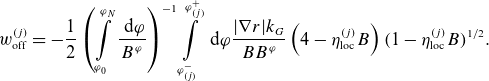 \begin{align} w_{\text{off}}^{(j)} = -\frac {1}{2} \left (\int \limits _{\varphi _0}^{\varphi _N}\frac {\textrm { d} \varphi }{B^\varphi }\right )^{-1} \int \limits _{\varphi _{(j)}^-}^{\varphi _{(j)}^+}\textrm { d} \varphi \frac {|\nabla r|k_G}{BB^\varphi } \left (4-\eta _{\textrm{loc}}^{(j)} B\right ) (1-\eta _{\textrm{loc}}^{(j)} B)^{1/2}. \end{align}
In field aligned Boozer coordinates, we replace $B^\varphi =B^2 (\iota B_\vartheta +B_\varphi )^{-1}$
with covariant field components being the flux functions, and use the last expression (2.6) for
$B^\varphi =B^2 (\iota B_\vartheta +B_\varphi )^{-1}$
with covariant field components being the flux functions, and use the last expression (2.6) for $|\nabla r|k_G$
to get
$|\nabla r|k_G$
to get
 \begin{align} w_{\text{off}}^{(j)} = \frac {\textrm { d} r}{\textrm { d} \psi } \left (\int \limits _{\varphi _0}^{\varphi _N}\frac {\textrm { d} \varphi }{B^2}\right )^{-1} I_{\mathcal{V}}^{(j)}, \qquad I_{\mathcal{V}}^{(j)} = \int \limits _{\varphi _{(j)}^-}^{\varphi _{(j)}^+} \textrm { d} \varphi \mathcal{V}, \end{align}
where
 \begin{align} \mathcal{V} = \frac {1}{2 B^3} \frac {\partial B}{\partial \vartheta _0} \left (4-\eta _{\textrm{loc}}^{(j)} B\right ) (1-\eta _{\textrm{loc}}^{(j)} B)^{1/2} =-\left [\frac {\partial }{\partial \vartheta _0} \frac {(1-\eta B)^{3/2}}{B^2}\right ]_{\eta =\eta _{\textrm{loc}}^{(j)}}. \end{align}
It should be noted that the off-set (3.54) ignores the contribution of the trapped–passing boundary layer, where the distribution function is the largest and strongly depends on $\varphi$
. This kind of off-set, which scales with the width of this layer,
$\varphi$
. This kind of off-set, which scales with the width of this layer, $\propto \nu ^{1/2}$
, is present also in axisymmetric devices and has been studied by Helander et al. (Reference Helander, Geiger and Maassberg2011).
$\propto \nu ^{1/2}$
, is present also in axisymmetric devices and has been studied by Helander et al. (Reference Helander, Geiger and Maassberg2011).
The result of (3.54) and (3.59) with $g^{(j)}_{\text{off}}$
obtained by propagator method (figure 17) is compared with the NEO-2 result in figure 19. For the configuration with
$g^{(j)}_{\text{off}}$
obtained by propagator method (figure 17) is compared with the NEO-2 result in figure 19. For the configuration with $\iota =1/4$
, the off-set is fully determined by the first (and last) off-set well,
$\iota =1/4$
, the off-set is fully determined by the first (and last) off-set well, $g^{(0)}_{\text{off}}$
, since
$g^{(0)}_{\text{off}}$
, since $g^{(1)}_{\text{off}}=0$
and
$g^{(1)}_{\text{off}}=0$
and $g^{(2)}_{\text{off}}=-g^{(0)}_{\text{off}}$
due to stellarator symmetry. For the configuration with
$g^{(2)}_{\text{off}}=-g^{(0)}_{\text{off}}$
due to stellarator symmetry. For the configuration with $\iota =2/5$
, both the off-set well,
$\iota =2/5$
, both the off-set well, $g^{(0)}_{\text{off}}$
, and the main region,
$g^{(0)}_{\text{off}}$
, and the main region, $g^{(1)}_{\text{off}}$
, are contributing (with
$g^{(1)}_{\text{off}}$
, are contributing (with $g^{(3)}_{\text{off}}=-g^{(1)}_{\text{off}}$
and
$g^{(3)}_{\text{off}}=-g^{(1)}_{\text{off}}$
and $g^{(4)}_{\text{off}}=-g^{(0)}_{\text{off}}$
just doubling the result due to stellarator symmetry). Off-set wells merge with the main regions (0 with 1 and 3 with 4) at
$g^{(4)}_{\text{off}}=-g^{(0)}_{\text{off}}$
just doubling the result due to stellarator symmetry). Off-set wells merge with the main regions (0 with 1 and 3 with 4) at $\nu _\ast \lt 10^{-4}$
, therefore we used
$\nu _\ast \lt 10^{-4}$
, therefore we used $\eta _{\textrm{loc}}^{(j)}$
for such combined regions in individual
$\eta _{\textrm{loc}}^{(j)}$
for such combined regions in individual $w^{(j)}_{\text{off}}$
. It can be seen that the contribution of the off-set wells is slightly larger than of the main regions, despite the much smaller toroidal extent, which is natural for bounce-averaged drift (the longer the orbit, the smaller is this drift). These two contributions tend to compensate for each other at lower collisionalities, which is a general trend due to the respective increase of the off-set domain length studied in more detail in § 4.2.
$w^{(j)}_{\text{off}}$
. It can be seen that the contribution of the off-set wells is slightly larger than of the main regions, despite the much smaller toroidal extent, which is natural for bounce-averaged drift (the longer the orbit, the smaller is this drift). These two contributions tend to compensate for each other at lower collisionalities, which is a general trend due to the respective increase of the off-set domain length studied in more detail in § 4.2.
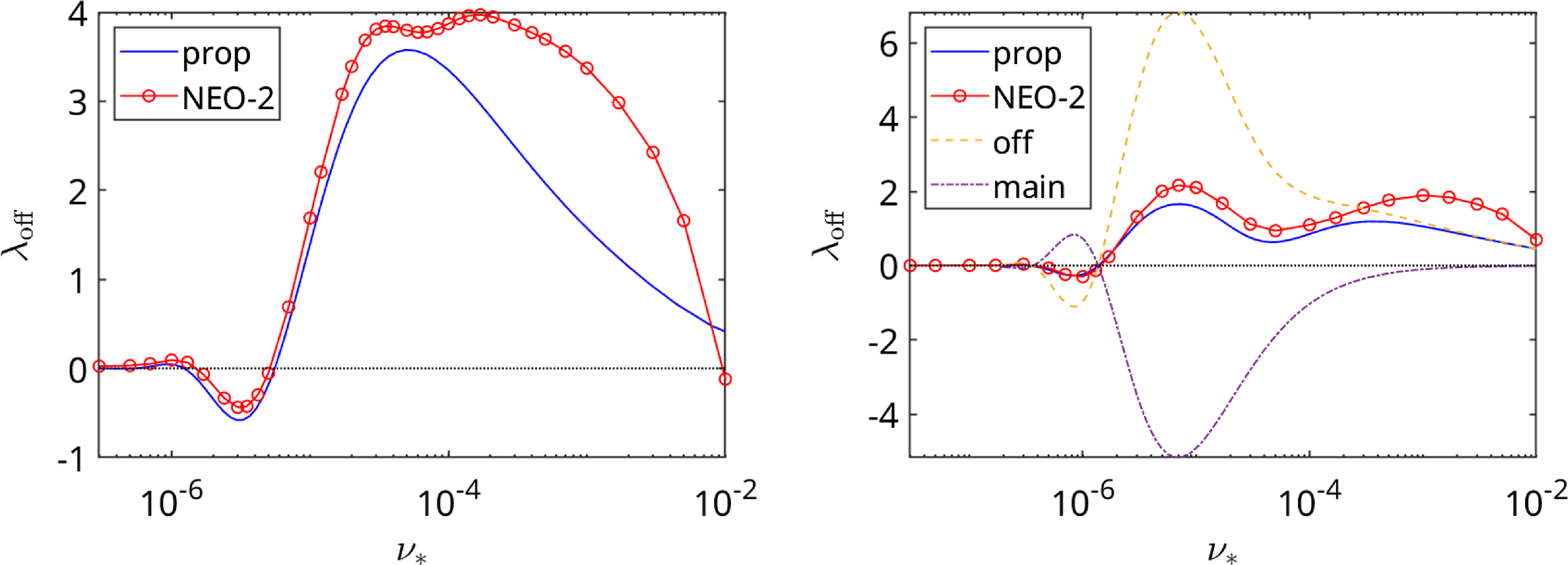
Figure 19. Off-set of the geometrical factor, $\lambda _{\text{off}}$
, from the propagator method via (3.54) (blue) and from NEO-2 results shown in figure 2 (red) for
$\lambda _{\text{off}}$
, from the propagator method via (3.54) (blue) and from NEO-2 results shown in figure 2 (red) for $\iota =1/4$
(left) and
$\iota =1/4$
(left) and $\iota =2/5$
(right). In the case of
$\iota =2/5$
(right). In the case of $\iota =2/5$
, also shown are summary contributions to (3.54) of the off-set domains (dashed) and of the main regions (dashed-dotted).
$\iota =2/5$
, also shown are summary contributions to (3.54) of the off-set domains (dashed) and of the main regions (dashed-dotted).
As it could be expected, relatively good agreement between the propagator method and NEO-2 is obtained at very low collisionalities while at $\nu _\ast \gt 10^{-4}$
direct off-set due to boundary layer discussed by Helander et al. (Reference Helander, Geiger and Maassberg2011) becomes also important.
$\nu _\ast \gt 10^{-4}$
direct off-set due to boundary layer discussed by Helander et al. (Reference Helander, Geiger and Maassberg2011) becomes also important.
4. Bootstrap/Ware-pinch off-set at irrational surfaces
As we have seen from the example of the ‘anti-sigma’ configuration in § 3.3, the Shaing–Callen limit cannot be reached in the case of perfectly aligned maxima where the bootstrap/Ware-pinch coefficient diverges as $1/\sqrt {\nu }$
. This, however, is the ideal case, which cannot be realized exactly. As follows from (3.53), due to the strong (
$1/\sqrt {\nu }$
. This, however, is the ideal case, which cannot be realized exactly. As follows from (3.53), due to the strong ( $1/\nu$
) scaling of maxima mis-alignment term with collisionality, sooner or later small mis-alignments of local maxima will prevail, and configuration will turn into a general one with a single global maximum. Therefore, we have to consider this general case now.
$1/\nu$
) scaling of maxima mis-alignment term with collisionality, sooner or later small mis-alignments of local maxima will prevail, and configuration will turn into a general one with a single global maximum. Therefore, we have to consider this general case now.
4.1. Long field lines
The field line integration technique employed in analytical asymptotic models and in NEO-2 assumes that the representative field line covers the flux surface densely enough so that the result does not depend on its length anymore. There are at least two ways to do so, in a way the ends of the field line are identical (and the solution is periodic) at the irrational surface. One way (standard in NEO-2) is to follow the line until there is a good match with the starting point, and then slightly modify $B(\varphi )$
in the last field period for a smooth field line closure. The result can be verified then by using another starting point at the same flux surface. Another way (employed here) is to replace
$B(\varphi )$
in the last field period for a smooth field line closure. The result can be verified then by using another starting point at the same flux surface. Another way (employed here) is to replace $\iota$
with a rational number of a high-order well approximating the original irrational
$\iota$
with a rational number of a high-order well approximating the original irrational $\iota$
and start from the global maximum. Thus, within stellarator symmetry, one can always keep quasi-Liouville’s theorem fulfilled exactly. Within this second approach, we consider now five different field lines for the magnetic field model used in § 2.3 with
$\iota$
and start from the global maximum. Thus, within stellarator symmetry, one can always keep quasi-Liouville’s theorem fulfilled exactly. Within this second approach, we consider now five different field lines for the magnetic field model used in § 2.3 with $\iota = 0.44 = 11/25$
,
$\iota = 0.44 = 11/25$
, $\iota = 0.43 = 43/100$
,
$\iota = 0.43 = 43/100$
, $\iota = 0.435 = 87/200$
,
$\iota = 0.435 = 87/200$
, $\iota = 0.438 = 219/500$
and
$\iota = 0.438 = 219/500$
and $\iota = 0.442 = 221/500$
which cover the field period with 75, 300, 600 and 1500 passes, respectively.
$\iota = 0.442 = 221/500$
which cover the field period with 75, 300, 600 and 1500 passes, respectively.
The resulting normalized bootstrap coefficients (2.44) are shown in figure 20. They are weakly dependent on $\iota$
for collisionalities
$\iota$
for collisionalities $\nu _\ast \gt 10^{-5}$
(in the first hill), and follow this trend down to
$\nu _\ast \gt 10^{-5}$
(in the first hill), and follow this trend down to $\nu _\ast = 10^{-6}$
in the second hill, with only the curve
$\nu _\ast = 10^{-6}$
in the second hill, with only the curve $\iota =0.43$
departing from the other four. As one can see from the
$\iota =0.43$
departing from the other four. As one can see from the $\iota$
scan in this figure, this transition is smooth, in contrast to the Shaing–Callen limit which shows well-known ‘bootstrap resonances’ briefly discussed in § 4.4. To analyze this behavior, we plot the Ware-pinch distribution function
$\iota$
scan in this figure, this transition is smooth, in contrast to the Shaing–Callen limit which shows well-known ‘bootstrap resonances’ briefly discussed in § 4.4. To analyze this behavior, we plot the Ware-pinch distribution function $g_{(3)}(\vartheta, \varphi, \lambda )$
(mono-energetic generalized Spitzer function) for particles with zero parallel velocity (
$g_{(3)}(\vartheta, \varphi, \lambda )$
(mono-energetic generalized Spitzer function) for particles with zero parallel velocity ( $\lambda =0$
) as function of angles for two cases of
$\lambda =0$
) as function of angles for two cases of $\iota =0.435$
and
$\iota =0.435$
and $\iota =0.43$
and two different collisionalities,
$\iota =0.43$
and two different collisionalities, $\nu _\ast = 3\cdot 10^{-4}$
(figure 21) and
$\nu _\ast = 3\cdot 10^{-4}$
(figure 21) and $\nu _\ast = 10^{-6}$
(figure 23). Since the distribution function in the trapped particle domain is almost independent of pitch parameter (equivalently of
$\nu _\ast = 10^{-6}$
(figure 23). Since the distribution function in the trapped particle domain is almost independent of pitch parameter (equivalently of $\eta$
), the plotted quantity characterizes well the radial particle flux. Obviously, this function is stellarator antisymmetric,
$\eta$
), the plotted quantity characterizes well the radial particle flux. Obviously, this function is stellarator antisymmetric, $g_{(3)}(\vartheta, \varphi, 0)=-g_{(3)}({-}\vartheta, -\varphi, 0)$
, and retains all other relevant features seen for the short field line examples in § 2.3.2. Namely, ‘hot spots’ around the global maximum (
$g_{(3)}(\vartheta, \varphi, 0)=-g_{(3)}({-}\vartheta, -\varphi, 0)$
, and retains all other relevant features seen for the short field line examples in § 2.3.2. Namely, ‘hot spots’ around the global maximum ( $\vartheta =\pi$
,
$\vartheta =\pi$
, $\varphi =\pi /3$
), where
$\varphi =\pi /3$
), where $g_{(3)}$
is the largest, correspond to the contact region with the boundary layer (see the left figure 7). These spots are responsible for the tokamak-like off-set studied by Helander et al. (Reference Helander, Geiger and Maassberg2011). One can clearly see in figure 21 also the off-set domains (blue and yellow) in the ripples adjacent to the global maximum (mainly contributing to the off-set at this collisionality) as well as the widely extending ‘main region’ (green). Thus, this case is rather similar to figure 6 for
$g_{(3)}$
is the largest, correspond to the contact region with the boundary layer (see the left figure 7). These spots are responsible for the tokamak-like off-set studied by Helander et al. (Reference Helander, Geiger and Maassberg2011). One can clearly see in figure 21 also the off-set domains (blue and yellow) in the ripples adjacent to the global maximum (mainly contributing to the off-set at this collisionality) as well as the widely extending ‘main region’ (green). Thus, this case is rather similar to figure 6 for $\nu _\ast = 10^{-4}$
. Remarkably, results for two different
$\nu _\ast = 10^{-4}$
. Remarkably, results for two different $\iota$
are almost indistinguishable, which explains the close values of
$\iota$
are almost indistinguishable, which explains the close values of $\lambda _{bB}$
in figure 20 at this collisionality. Since the radial guiding center velocity
$\lambda _{bB}$
in figure 20 at this collisionality. Since the radial guiding center velocity $v_g^r$
is stellarator antisymmetric as well, the resulting normalized radial trapped particle flux distribution over the angles
$v_g^r$
is stellarator antisymmetric as well, the resulting normalized radial trapped particle flux distribution over the angles $\gamma$
given with good accuracy by
$\gamma$
given with good accuracy by $\gamma (\vartheta, \varphi ) = \mathcal{V} (\vartheta, \varphi ) g_{(3)}(\vartheta, \varphi, 0)$
, where
$\gamma (\vartheta, \varphi ) = \mathcal{V} (\vartheta, \varphi ) g_{(3)}(\vartheta, \varphi, 0)$
, where $\mathcal{V}$
is the sub-integrand in (3.59), is stellarator symmetric. It is shown for
$\mathcal{V}$
is the sub-integrand in (3.59), is stellarator symmetric. It is shown for $\nu _\ast = 3\cdot 10^{-4}$
in figure 22, where the contribution of the off-set domain (
$\nu _\ast = 3\cdot 10^{-4}$
in figure 22, where the contribution of the off-set domain ( $2 \lt \vartheta \lt 4$
) is positive, which agrees with the first hill in figure 20. Note that the direct contribution of the boundary layer is already small at this collisionality, which is also seen from vanishing hot spots in figure 22.
$2 \lt \vartheta \lt 4$
) is positive, which agrees with the first hill in figure 20. Note that the direct contribution of the boundary layer is already small at this collisionality, which is also seen from vanishing hot spots in figure 22.
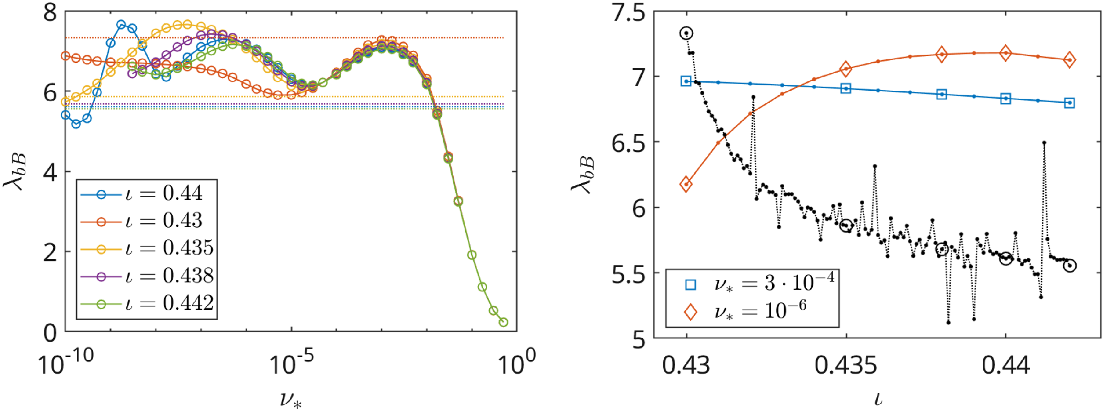
Figure 20. Normalized bootstrap coefficient (2.44) for five $\iota$
values vs. normalized collisionality
$\iota$
values vs. normalized collisionality $\nu _\ast$
(left) and its dependence on
$\nu _\ast$
(left) and its dependence on $\iota$
for two selected collisionalities shown in the legend (right). Shaing–Callen limit (2.43) is shown with dotted lines (data points – with dots). Abscissa values for markers in the right plot correspond to the legend in the left plot.
$\iota$
for two selected collisionalities shown in the legend (right). Shaing–Callen limit (2.43) is shown with dotted lines (data points – with dots). Abscissa values for markers in the right plot correspond to the legend in the left plot.

Figure 21. Generalized Spitzer function $g_{(3)}(\vartheta, \varphi, \lambda )$
for standing particles (
$g_{(3)}(\vartheta, \varphi, \lambda )$
for standing particles ( $\lambda =0$
) at the flux surface with
$\lambda =0$
) at the flux surface with $\iota =0.435$
(left) and
$\iota =0.435$
(left) and $\iota =0.43$
(right) for
$\iota =0.43$
(right) for $\nu _\ast = 3\cdot 10^{-4}$
. White dotted lines show the field line starting from the global maximum and making 7 toroidal turns.
$\nu _\ast = 3\cdot 10^{-4}$
. White dotted lines show the field line starting from the global maximum and making 7 toroidal turns.
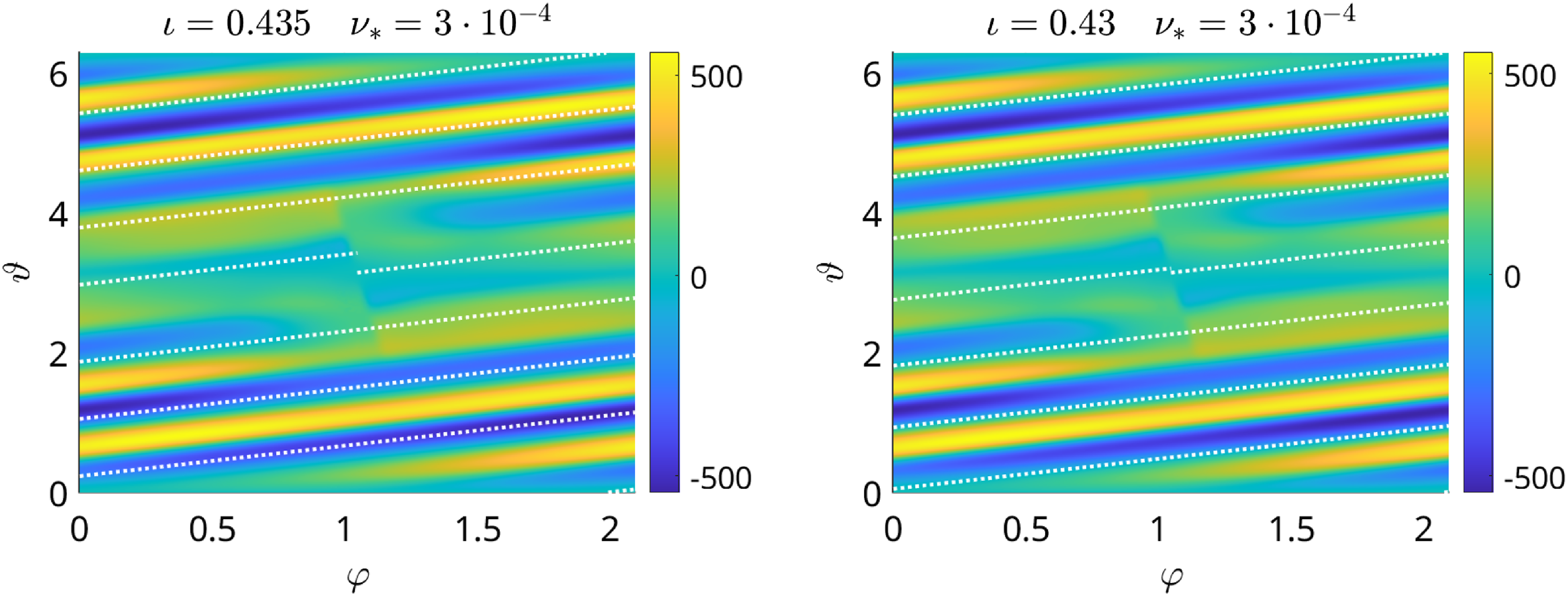
Figure 22. Normalized distribution over the angles of trapped particle radial flux $\gamma (\vartheta, \varphi )$
at the flux surface with
$\gamma (\vartheta, \varphi )$
at the flux surface with $\iota =0.435$
(left) and
$\iota =0.435$
(left) and $\iota =0.43$
(right) for
$\iota =0.43$
(right) for $\nu _\ast = 3\cdot 10^{-4}$
. White dotted lines – the same as in figure 21.
$\nu _\ast = 3\cdot 10^{-4}$
. White dotted lines – the same as in figure 21.
Off-set in adjacent toroidal ripples vanishes completely for the lower collisionality case $\nu _\ast = 10^{-6}$
shown in figure 23. The visible difference between
$\nu _\ast = 10^{-6}$
shown in figure 23. The visible difference between $\iota =0.435$
and
$\iota =0.435$
and $\iota =0.43$
is different amplitudes of straps on
$\iota =0.43$
is different amplitudes of straps on $g_{(3)}$
which, in fact, is higher for
$g_{(3)}$
which, in fact, is higher for $\iota =0.43$
where the off-set of
$\iota =0.43$
where the off-set of $\lambda _{bB}$
is smaller (see figure 20). Less visible is the split of the straps into the off-set domain and the main region for
$\lambda _{bB}$
is smaller (see figure 20). Less visible is the split of the straps into the off-set domain and the main region for $\iota =0.435$
. Actually, this split is responsible for the lower amplitude of the straps in this case. Note that the strap structure and difference in its amplitude for two
$\iota =0.435$
. Actually, this split is responsible for the lower amplitude of the straps in this case. Note that the strap structure and difference in its amplitude for two $\iota$
values transfers also to the angular distribution of radial particle flux shown in figure 24. Despite the factor 1.5 higher amplitude of the flux density modulation, the value of
$\iota$
values transfers also to the angular distribution of radial particle flux shown in figure 24. Despite the factor 1.5 higher amplitude of the flux density modulation, the value of $\lambda _{bB}$
is only 14 % different (and is lower) for
$\lambda _{bB}$
is only 14 % different (and is lower) for $\iota =0.43$
than for
$\iota =0.43$
than for $\iota =0.435$
. The reason is the relatively low contribution of the strap structure dominating the plot to the radial transport because this contribution is mostly averaged to zero. Namely, change of
$\iota =0.435$
. The reason is the relatively low contribution of the strap structure dominating the plot to the radial transport because this contribution is mostly averaged to zero. Namely, change of $g_{(3)}$
along the straps (more precisely, along the field lines) is rather slow, but not slow is the change of local guiding center velocity which, at the end, results in much smaller bounce-averaged value actually contributing to the flux.
$g_{(3)}$
along the straps (more precisely, along the field lines) is rather slow, but not slow is the change of local guiding center velocity which, at the end, results in much smaller bounce-averaged value actually contributing to the flux.
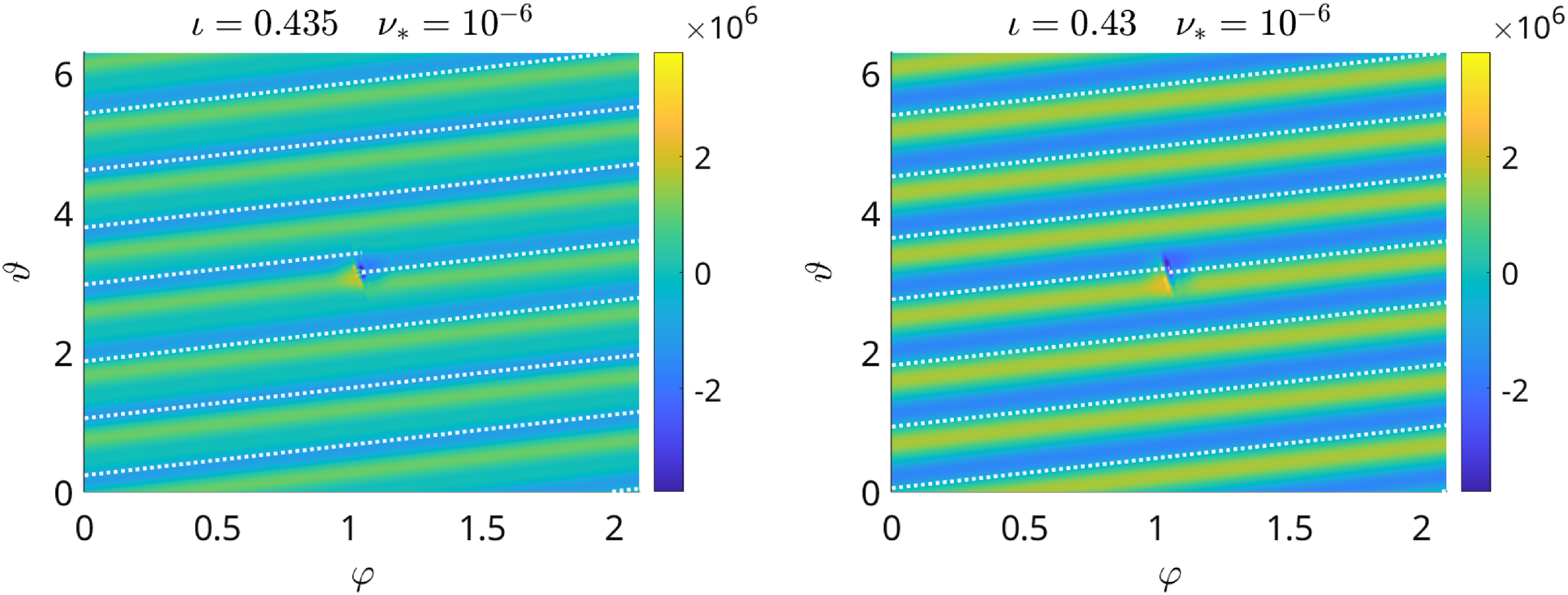
Figure 23. The same as figure 21 for $\nu _\ast = 10^{-6}$
.
$\nu _\ast = 10^{-6}$
.
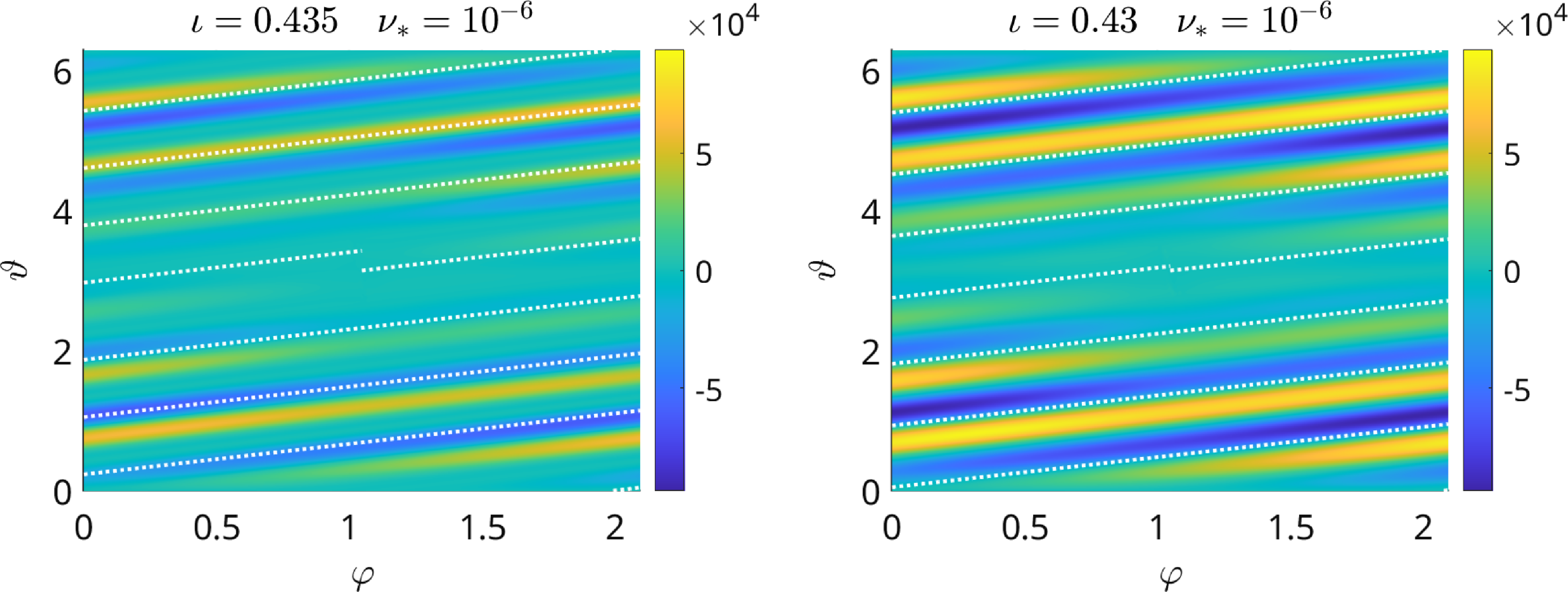
Figure 24. The same as figure 22 for $\nu _\ast = 10^{-6}$
.
$\nu _\ast = 10^{-6}$
.
The appearance of strap structure on the generalized Spitzer function $g_{(3)}$
, which only emerges in figure 21 and becomes dominant in figure 23, is connected with a certain paradox of the asymptotic solution of Helander et al. (Reference Helander, Geiger and Maassberg2011) for trapped particles,
$g_{(3)}$
, which only emerges in figure 21 and becomes dominant in figure 23, is connected with a certain paradox of the asymptotic solution of Helander et al. (Reference Helander, Geiger and Maassberg2011) for trapped particles, $g_0^t$
, given by (2.47) in § 2.2.2. Being perfectly correct and accurately reproduced at short field lines and the lowest collisionalities by NEO-2, it does not result in smooth distributions over irrational flux surfaces, but rather in the fractal structure with an infinite amplitude. Since two arbitrarily close points on the flux surface can be connected in the
$g_0^t$
, given by (2.47) in § 2.2.2. Being perfectly correct and accurately reproduced at short field lines and the lowest collisionalities by NEO-2, it does not result in smooth distributions over irrational flux surfaces, but rather in the fractal structure with an infinite amplitude. Since two arbitrarily close points on the flux surface can be connected in the $1/\nu$
regime only along the field line, the connecting segment of the field line is in general infinite, which results in infinite values of the integral (2.47). As we saw already in § 2.3.2, this paradox is resolved for finite collisionality. Namely, whenever the field line enters the ‘hot spot’ (boundary layer), it starts a new segment which should be treated independently from the rest. Thus, the problem becomes local at finite collisionalities even at the irrational surfaces. With reducing
$1/\nu$
regime only along the field line, the connecting segment of the field line is in general infinite, which results in infinite values of the integral (2.47). As we saw already in § 2.3.2, this paradox is resolved for finite collisionality. Namely, whenever the field line enters the ‘hot spot’ (boundary layer), it starts a new segment which should be treated independently from the rest. Thus, the problem becomes local at finite collisionalities even at the irrational surfaces. With reducing $\nu _\ast$
the size of the ‘hot spot’ is reduced, and, at some point there will be a transition from a 7 strap structure to another structure with more straps. Finally, in the zero collisionality limit, the fractal structure of the solution of Helander et al. (Reference Helander, Geiger and Maassberg2011) will be recovered. Of course, within this simple splitting approach combined with an asymptotic model, the fractal structure will not appear anymore but the off-set effect will naturally be different from the one in the collisional model.
$\nu _\ast$
the size of the ‘hot spot’ is reduced, and, at some point there will be a transition from a 7 strap structure to another structure with more straps. Finally, in the zero collisionality limit, the fractal structure of the solution of Helander et al. (Reference Helander, Geiger and Maassberg2011) will be recovered. Of course, within this simple splitting approach combined with an asymptotic model, the fractal structure will not appear anymore but the off-set effect will naturally be different from the one in the collisional model.
The actual ‘splitting’ of the collisional solution for $\nu _\ast = 3\cdot 10^{-4}$
is shown in figure 25, where the same distribution functions as in figure 21 are plotted along two field lines as functions of the number of toroidal turns
$\nu _\ast = 3\cdot 10^{-4}$
is shown in figure 25, where the same distribution functions as in figure 21 are plotted along two field lines as functions of the number of toroidal turns $(\varphi -\varphi _0)/(2\pi )$
. The first line starts from the global maximum
$(\varphi -\varphi _0)/(2\pi )$
. The first line starts from the global maximum $(\vartheta _0,\varphi _0)=(\pi, \pi /3)$
, and the second one starts from the close point with
$(\vartheta _0,\varphi _0)=(\pi, \pi /3)$
, and the second one starts from the close point with $\vartheta =\vartheta _0+\delta \vartheta$
. Together with solutions of NEO-2 for two
$\vartheta =\vartheta _0+\delta \vartheta$
. Together with solutions of NEO-2 for two $\iota$
values, also plotted is the asymptotic solution of Helander et al. (Reference Helander, Geiger and Maassberg2011), (2.47), which has the form of a straight line in Boozer coordinates,
$\iota$
values, also plotted is the asymptotic solution of Helander et al. (Reference Helander, Geiger and Maassberg2011), (2.47), which has the form of a straight line in Boozer coordinates, $g_0^t =(\iota B_\vartheta + B_\varphi )(\varphi -\varphi _0)$
. In the left plot, one can observe the same pattern consisting of the ‘main region’ and two off-set domains (this case is similar to the one in figure 6) repeated three times, which corresponds to a ‘resonance’ with
$g_0^t =(\iota B_\vartheta + B_\varphi )(\varphi -\varphi _0)$
. In the left plot, one can observe the same pattern consisting of the ‘main region’ and two off-set domains (this case is similar to the one in figure 6) repeated three times, which corresponds to a ‘resonance’ with $\iota = 3/7$
(note that
$\iota = 3/7$
(note that $0.435 -3/7 \approx 0.0064$
and
$0.435 -3/7 \approx 0.0064$
and $0.43 -3/7 \approx 0.0014$
). One can also see that
$0.43 -3/7 \approx 0.0014$
). One can also see that $g_0^t$
well represents the solution within each domain up to a constant shift introduced by splitting in the boundary layers. Spikes on
$g_0^t$
well represents the solution within each domain up to a constant shift introduced by splitting in the boundary layers. Spikes on $g_{(3)}$
correspond to the contact with the trapped–passing boundary layer (‘hot spots’), and one can see nearly no spikes at the transitions between the off-set domains and the main region, which correspond to the boundary layers between trapped particle classes. One can also see slow accumulation of a different type of off-set in the main regions, which results in a different
$g_{(3)}$
correspond to the contact with the trapped–passing boundary layer (‘hot spots’), and one can see nearly no spikes at the transitions between the off-set domains and the main region, which correspond to the boundary layers between trapped particle classes. One can also see slow accumulation of a different type of off-set in the main regions, which results in a different $g_{(3)}$
pattern in the long run (see the right plot). This off-set, however, has a much smaller effect on
$g_{(3)}$
pattern in the long run (see the right plot). This off-set, however, has a much smaller effect on $\lambda _{bB}$
(see figure 20) because the bounce-averaged velocity for relatively long ‘main regions’ is much smaller than for the short off-set domains.
$\lambda _{bB}$
(see figure 20) because the bounce-averaged velocity for relatively long ‘main regions’ is much smaller than for the short off-set domains.
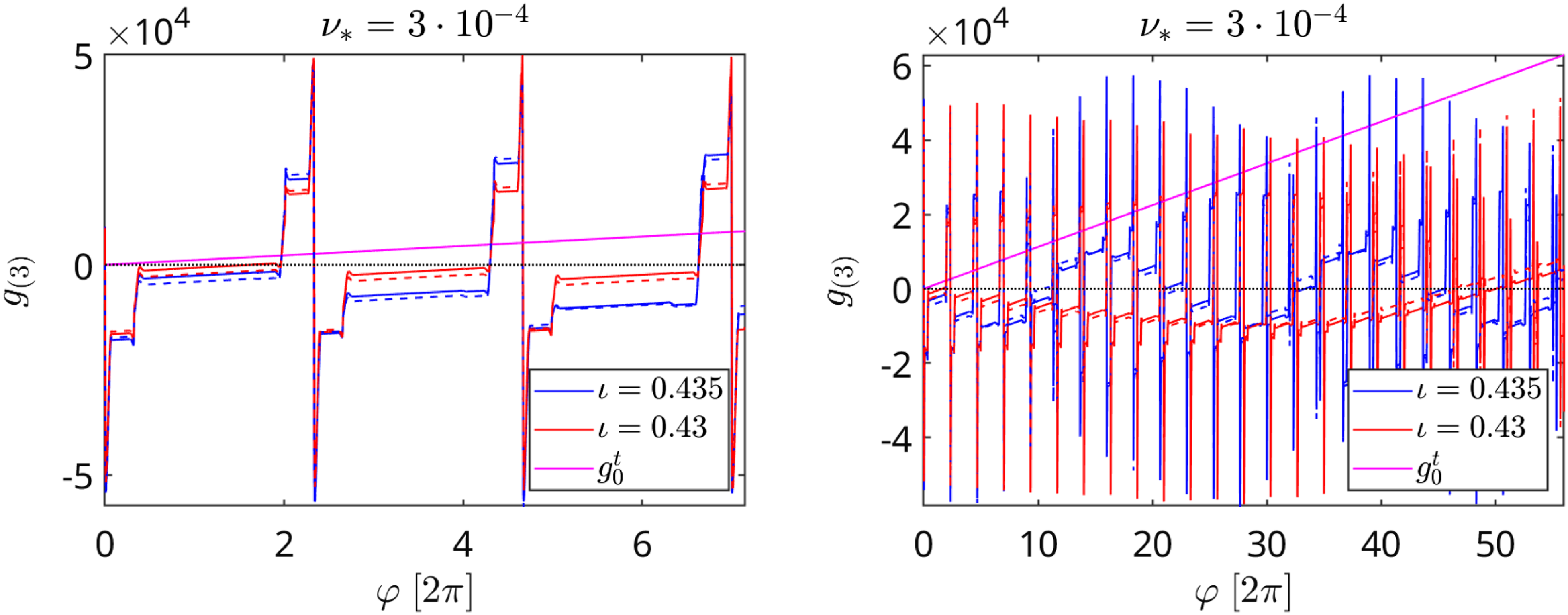
Figure 25. Generalized Spitzer function $g_{(3)}$
along the field line starting from global maximum (solid) and from the close point displaced by
$g_{(3)}$
along the field line starting from global maximum (solid) and from the close point displaced by $\Delta \vartheta = 0.03$
(dashed) for
$\Delta \vartheta = 0.03$
(dashed) for $\iota = 0.435$
(blue) and
$\iota = 0.435$
(blue) and $\iota = 0.43$
(red) and
$\iota = 0.43$
(red) and $\nu _\ast = 3\cdot 10^{-4}$
. The magenta line shows the asymptotic solution
$\nu _\ast = 3\cdot 10^{-4}$
. The magenta line shows the asymptotic solution $g_0^t$
, (2.47), at the first field line. Left and right plots show the same for 7 and 56 periods, respectively.
$g_0^t$
, (2.47), at the first field line. Left and right plots show the same for 7 and 56 periods, respectively.
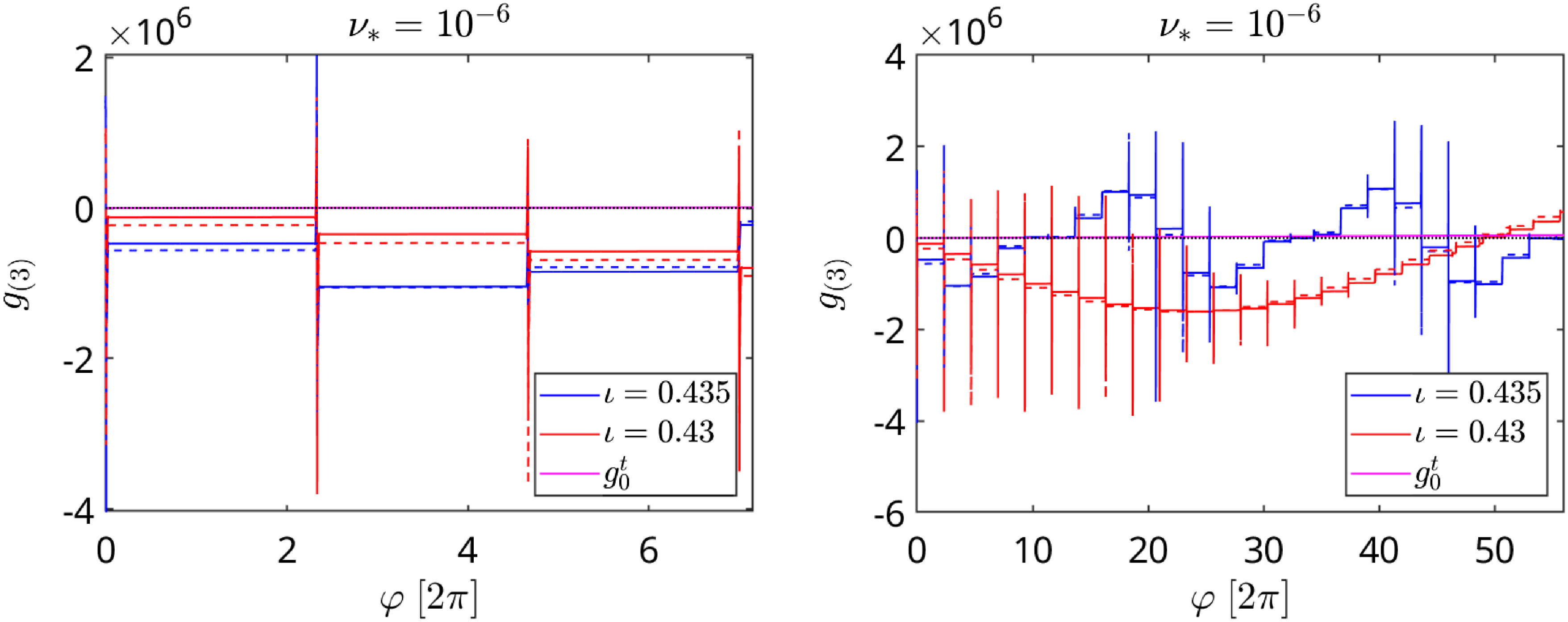
Figure 26. The same as figure 25 for $\nu _\ast = 10^{-6}$
and
$\nu _\ast = 10^{-6}$
and $\Delta \vartheta = 0.01$
.
$\Delta \vartheta = 0.01$
.
Short off-set domains fully disappear at lower collisionality $\nu _\ast = 10^{-6}$
, as shown in figure 26. There, the off-set pattern in the long run determines
$\nu _\ast = 10^{-6}$
, as shown in figure 26. There, the off-set pattern in the long run determines $\lambda _{bB}$
, which shows then in figure 20 a significant difference for the two
$\lambda _{bB}$
, which shows then in figure 20 a significant difference for the two $\iota$
values under examination here. We see that this pattern is formed by sub-domains with toroidal extent corresponding to a full poloidal turn of the field line. For the case
$\iota$
values under examination here. We see that this pattern is formed by sub-domains with toroidal extent corresponding to a full poloidal turn of the field line. For the case $\iota =0.435$
, the pattern is repeated twice in the long run and is formed by the ‘main region’ consisting of 3 sub-domains (field line misses the boundary layer during these full poloidal turns), and there are 3 off-set domains on each side of the main region with the opposite off-set value in each triple (field line visits the boundary layer within these sub-domains at opposite sides for each triple). One can see also ‘symmetric’ sub-domains with nearly no off-set, which separate the patterns approximately repeated after 25 toroidal turns. In contrast, for
$\iota =0.435$
, the pattern is repeated twice in the long run and is formed by the ‘main region’ consisting of 3 sub-domains (field line misses the boundary layer during these full poloidal turns), and there are 3 off-set domains on each side of the main region with the opposite off-set value in each triple (field line visits the boundary layer within these sub-domains at opposite sides for each triple). One can see also ‘symmetric’ sub-domains with nearly no off-set, which separate the patterns approximately repeated after 25 toroidal turns. In contrast, for $\iota =0.43$
, almost a harmonic structure is formed with a period determined by
$\iota =0.43$
, almost a harmonic structure is formed with a period determined by $\Delta \iota = 0.44 - 0.43 = 0.01$
.
$\Delta \iota = 0.44 - 0.43 = 0.01$
.
Finally, the normalized trapped particle radial flux distribution over the angles $\gamma = \mathcal{V} g_{(3)}$
(the same quantity as in figure 24) and the sub-domain average
$\gamma = \mathcal{V} g_{(3)}$
(the same quantity as in figure 24) and the sub-domain average $\bar \gamma = \langle \mathcal{V} \rangle _{\vartheta } g_{(3)}$
m where
$\bar \gamma = \langle \mathcal{V} \rangle _{\vartheta } g_{(3)}$
m where $ \langle \mathcal{V} \rangle _{\vartheta }$
are averages over the field line segments corresponding to one poloidal turn (i.e. these are integrals in (3.59) normalized by
$ \langle \mathcal{V} \rangle _{\vartheta }$
are averages over the field line segments corresponding to one poloidal turn (i.e. these are integrals in (3.59) normalized by $\varphi _{j+1}-\varphi _j$
with
$\varphi _{j+1}-\varphi _j$
with $[\varphi _j,\varphi _{j+1}]$
being the sub-domain) are shown in figure 27 for the same field lines as in figure 26 and
$[\varphi _j,\varphi _{j+1}]$
being the sub-domain) are shown in figure 27 for the same field lines as in figure 26 and $\nu _\ast = 10^{-6}$
. It can be seen that large oscillations on the local flux density
$\nu _\ast = 10^{-6}$
. It can be seen that large oscillations on the local flux density $\gamma$
are mostly averaged off within sub-domains, and the resulting sub-domain average
$\gamma$
are mostly averaged off within sub-domains, and the resulting sub-domain average $\bar \gamma$
which is determined mainly by the bounce-averaged radial drift shows the significant positive contribution of the off-set domains for
$\bar \gamma$
which is determined mainly by the bounce-averaged radial drift shows the significant positive contribution of the off-set domains for $\iota = 0.435$
and a smaller negative contribution for
$\iota = 0.435$
and a smaller negative contribution for $\iota = 0.43$
(in agreement with the trend in figure 20).
$\iota = 0.43$
(in agreement with the trend in figure 20).
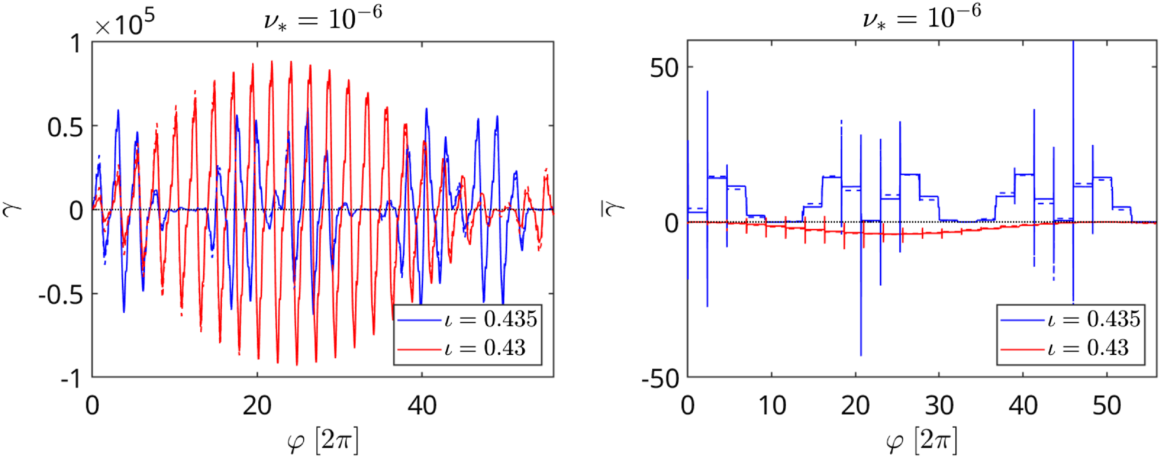
Figure 27. Normalized trapped particle radial flux angular density $\gamma$
(left) and sub-domain average
$\gamma$
(left) and sub-domain average $\bar \gamma$
(right) for the distribution functions shown in figure 26.
$\bar \gamma$
(right) for the distribution functions shown in figure 26.
4.2. Asymptotic behavior at irrational surfaces
For estimation of the $\lambda _{bB}$
trend with
$\lambda _{bB}$
trend with $\nu _\ast \rightarrow 0$
we analyze the nearly periodic pattern seen in right plots of figures 26 and 27 (such a pattern is seen also in the left plot of figure 25 while the right plot shows the overlay of two patterns). This pattern is formed if the field line starting in close vicinity to the global maximum point
$\nu _\ast \rightarrow 0$
we analyze the nearly periodic pattern seen in right plots of figures 26 and 27 (such a pattern is seen also in the left plot of figure 25 while the right plot shows the overlay of two patterns). This pattern is formed if the field line starting in close vicinity to the global maximum point $(\vartheta _{\textrm{max}},\varphi _{\textrm{max}})$
, i.e. at the point
$(\vartheta _{\textrm{max}},\varphi _{\textrm{max}})$
, i.e. at the point $(\vartheta _0,\varphi _0)=(\vartheta _{\textrm{max}}+\Delta \vartheta _0,\varphi _{\textrm{max}})$
where
$(\vartheta _0,\varphi _0)=(\vartheta _{\textrm{max}}+\Delta \vartheta _0,\varphi _{\textrm{max}})$
where $\Delta \vartheta _0 \ll \delta \vartheta$
and
$\Delta \vartheta _0 \ll \delta \vartheta$
and $\delta \vartheta$
is the poloidal boundary layer width (width of ‘hot spots’ in figures 21 and 23), returns after
$\delta \vartheta$
is the poloidal boundary layer width (width of ‘hot spots’ in figures 21 and 23), returns after $N$
turns back to this vicinity,
$N$
turns back to this vicinity, $(\vartheta _N,\varphi _N)=(\vartheta _{\textrm{max}}+\Delta \vartheta _N,\varphi _{\textrm{max}})$
with
$(\vartheta _N,\varphi _N)=(\vartheta _{\textrm{max}}+\Delta \vartheta _N,\varphi _{\textrm{max}})$
with $\Delta \vartheta _N \ll \delta \vartheta$
. The off-set pattern is formed if within these
$\Delta \vartheta _N \ll \delta \vartheta$
. The off-set pattern is formed if within these $N$
turns at least one approximate match occurs at some
$N$
turns at least one approximate match occurs at some $(\vartheta, \varphi )=(\vartheta _{\textrm{max}}+\Delta \vartheta, \varphi _{\textrm{max}})$
with
$(\vartheta, \varphi )=(\vartheta _{\textrm{max}}+\Delta \vartheta, \varphi _{\textrm{max}})$
with $\Delta \vartheta _0 \ll \Delta \vartheta \leqslant \delta \vartheta$
. By the symmetry argument (one can make
$\Delta \vartheta _0 \ll \Delta \vartheta \leqslant \delta \vartheta$
. By the symmetry argument (one can make $N$
turns backwards), such matches come in pairs, thus forming one ‘main region’ and at least two off-set domains with positive and negative off-sets, respectively (see the left plot in figure 25 and the right plots in figures 26 and 27 where six off-set domains are formed for
$N$
turns backwards), such matches come in pairs, thus forming one ‘main region’ and at least two off-set domains with positive and negative off-sets, respectively (see the left plot in figure 25 and the right plots in figures 26 and 27 where six off-set domains are formed for $\iota =0.435$
).
$\iota =0.435$
).
Expanding the magnetic field around the global maximum point
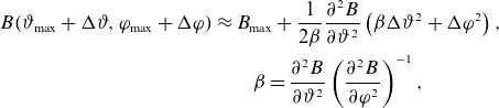 \begin{align} B(\vartheta _{\textrm{max}}+\Delta \vartheta, \varphi _{\textrm{max}}+\Delta \varphi ) & \approx B_{\textrm{max}} +\frac {1}{2\beta }\frac {\partial ^2 B}{\partial \vartheta ^2}\left (\beta \Delta \vartheta ^2+\Delta \varphi ^2\right ), \nonumber \\ & \qquad \beta =\frac {\partial ^2B}{\partial \vartheta ^2}\left (\frac {\partial ^2B}{\partial \varphi ^2}\right )^{-1}, \end{align}
where the second derivatives correspond to the global maximum point, and the mixed derivative there is zero for our example (2.57), we can relate the distance $\Delta \eta$
between class-transition boundary
$\Delta \eta$
between class-transition boundary $\eta =\eta _c=1/B^{\textrm{loc}}_{\textrm{max}}$
and trapped–passing boundary
$\eta =\eta _c=1/B^{\textrm{loc}}_{\textrm{max}}$
and trapped–passing boundary $\eta =\eta _b=1/B_{\textrm{max}}$
to the poloidal distance
$\eta =\eta _b=1/B_{\textrm{max}}$
to the poloidal distance $\Delta \vartheta$
between the respective local maximum and the global maximum as
$\Delta \vartheta$
between the respective local maximum and the global maximum as
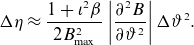 \begin{align} \Delta \eta \approx \frac {1+\iota ^2\beta }{2 B_{\textrm{max}}^2}\left |\frac {\partial ^2B}{\partial \vartheta ^2}\right |\Delta \vartheta ^2. \end{align}
We have expressed here the toroidal distance between these maxima as $\Delta \varphi =-\iota \beta \Delta \vartheta$
, which follows from the local maximum condition
$\Delta \varphi =-\iota \beta \Delta \vartheta$
, which follows from the local maximum condition $\textbf {h}\cdot \nabla B = 0$
and (4.1). Assuming that rational numbers
$\textbf {h}\cdot \nabla B = 0$
and (4.1). Assuming that rational numbers $0\lt m/n \lt 1$
with
$0\lt m/n \lt 1$
with $n\lt N_{\textrm{max}}$
are distributed uniformly in this interval (which is generally not true but gives a correct order of magnitude estimate), we obtain for the best match at some
$n\lt N_{\textrm{max}}$
are distributed uniformly in this interval (which is generally not true but gives a correct order of magnitude estimate), we obtain for the best match at some $n=N$
that
$n=N$
that
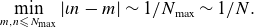 \begin{align} \min \limits _{m,n\leqslant N_{\textrm{max}}}|\iota n-m| \sim 1/N_{\textrm{max}} \sim 1/N. \end{align}
Thus, a field line starting at a global maximum will be displaced from this maximum after $N$
toroidal turns by
$N$
toroidal turns by $\Delta \vartheta _N \sim 2\pi /N$
and, according to (4.2), pass through the local maximum with respective class boundary
$\Delta \vartheta _N \sim 2\pi /N$
and, according to (4.2), pass through the local maximum with respective class boundary $\eta _c$
displacement
$\eta _c$
displacement $\Delta \eta _N=\eta _c-\eta _b$
given by
$\Delta \eta _N=\eta _c-\eta _b$
given by
 \begin{align} \Delta \eta _N \approx \frac {2 \pi ^2 \varepsilon _t\eta _b}{N^2}, \end{align}
where we denoted $\varepsilon _t \equiv (1+\iota ^2\beta )\eta _b\left |\partial ^2 B /\partial \vartheta ^2\right |$
well represented by field modulation in an axisymmetric tokamak. The trapped–passing boundary layer width corresponding to
$\varepsilon _t \equiv (1+\iota ^2\beta )\eta _b\left |\partial ^2 B /\partial \vartheta ^2\right |$
well represented by field modulation in an axisymmetric tokamak. The trapped–passing boundary layer width corresponding to $N$
toroidal turns is given by (3.20) with
$N$
toroidal turns is given by (3.20) with $\varphi =\varphi _0$
and
$\varphi =\varphi _0$
and $\varphi ^\prime =\varphi _0+2\pi N$
resulting in the estimate
$\varphi ^\prime =\varphi _0+2\pi N$
resulting in the estimate
 \begin{align} \delta \eta \approx 4 \pi ^{-1/2}(2\varepsilon _t)^{1/4}\eta _b\left (\nu _\ast N\right )^{1/2}, \end{align}
obtained here for $\varepsilon _M \ll \varepsilon _t \ll 1$
(see (2.57)) and using
$\varepsilon _M \ll \varepsilon _t \ll 1$
(see (2.57)) and using $\iota B_\vartheta +B_\varphi \approx R/\eta _b$
. Since the poloidal width of the boundary layer
$\iota B_\vartheta +B_\varphi \approx R/\eta _b$
. Since the poloidal width of the boundary layer $\delta \vartheta$
and boundary layer width
$\delta \vartheta$
and boundary layer width $\delta \eta$
are related by (4.2) with replacement
$\delta \eta$
are related by (4.2) with replacement $\Delta \rightarrow \delta$
, the best match after
$\Delta \rightarrow \delta$
, the best match after $N$
turns completing the off-set pattern means
$N$
turns completing the off-set pattern means $\Delta \eta _N \ll \delta \eta$
, which, according to (4.4) and (4.5), results in
$\Delta \eta _N \ll \delta \eta$
, which, according to (4.4) and (4.5), results in
 \begin{align} N \gg \frac {\pi \varepsilon _t^{3/10}}{\sqrt {2}\nu _\ast ^{1/5}}, \qquad \delta \eta \gg 4 \eta _b \left (\varepsilon _t \nu _\ast \right )^{2/5}. \end{align}
The last expression (4.6) agrees with the $\nu _\ast$
scaling of the boundary layer width obtained by a similar argument in Helander, Parra & Newton (Reference Helander, Parra and Newton2017). Since
$\nu _\ast$
scaling of the boundary layer width obtained by a similar argument in Helander, Parra & Newton (Reference Helander, Parra and Newton2017). Since $\Delta \eta _N/\delta \eta \sim N^{-5/2}$
rapidly decays with
$\Delta \eta _N/\delta \eta \sim N^{-5/2}$
rapidly decays with $N$
, strong inequality (4.6) is achieved even if one only doubles the
$N$
, strong inequality (4.6) is achieved even if one only doubles the $N$
value given by the right-hand side. Therefore, we use (4.6) further, as order of magnitude estimates rather than strong conditions. Assuming for simplicity then only one pair of off-set domains is formed with local minimum mis-match of the order of the boundary layer width in the main region,
$N$
value given by the right-hand side. Therefore, we use (4.6) further, as order of magnitude estimates rather than strong conditions. Assuming for simplicity then only one pair of off-set domains is formed with local minimum mis-match of the order of the boundary layer width in the main region, $\Delta \eta \sim \delta \eta _{\text{ref}}$
and estimating this width in the large aspect ratio limit as
$\Delta \eta \sim \delta \eta _{\text{ref}}$
and estimating this width in the large aspect ratio limit as $\delta \eta _{\text{ref}} \sim \delta \eta \sim 4 \eta _b \left (\varepsilon _t \nu _\ast \right )^{2/5}$
, we obtain the distribution function in the off-set domains with the help of (3.52), (3.46) and estimate
$\delta \eta _{\text{ref}} \sim \delta \eta \sim 4 \eta _b \left (\varepsilon _t \nu _\ast \right )^{2/5}$
, we obtain the distribution function in the off-set domains with the help of (3.52), (3.46) and estimate $\alpha ^\pm _{mr} \sim 1$
due to
$\alpha ^\pm _{mr} \sim 1$
due to $x_{\pm 0} \sim \Delta \eta /\delta \eta _{\text{ref}} \sim 1$
as
$x_{\pm 0} \sim \Delta \eta /\delta \eta _{\text{ref}} \sim 1$
as
 \begin{align} g_{\text{off}}^{(j)} \sim R B_0 \varepsilon _t^{-1/10} \nu _\ast ^{-3/5}, \end{align}
where $B_0=B_{\textrm{max}}$
, and constant (3.18) has been estimated as
$B_0=B_{\textrm{max}}$
, and constant (3.18) has been estimated as $C_0 \sim R B_0^2 /(\nu _\ast \varepsilon _t^{1/2})$
. Note that scaling (4.7) is reproduced up to a factor 2 by the relation between the color ranges in figures 21 and 23 and is in good agreement with collisionality dependence of the span
$C_0 \sim R B_0^2 /(\nu _\ast \varepsilon _t^{1/2})$
. Note that scaling (4.7) is reproduced up to a factor 2 by the relation between the color ranges in figures 21 and 23 and is in good agreement with collisionality dependence of the span $g_{\text{off}}^{\text{(sp)}}$
of the generalized Spitzer function which corresponds to the maximum off-set at
$g_{\text{off}}^{\text{(sp)}}$
of the generalized Spitzer function which corresponds to the maximum off-set at $\varphi =0$
line (in particular, in figures 21 and 23), see figure 28.
$\varphi =0$
line (in particular, in figures 21 and 23), see figure 28.
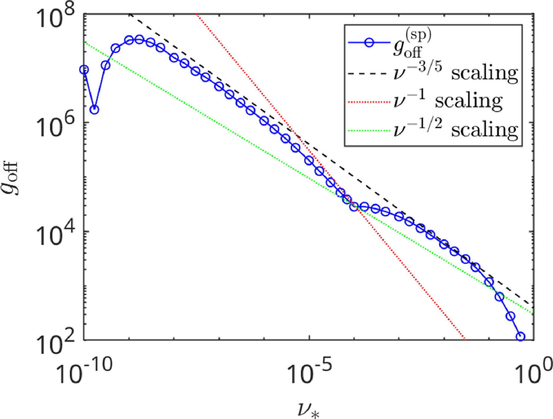
Figure 28. Span of the generalized Spitzer function $g_{\text{off}}^{\text{(sp)}}\equiv (\!\max (g_{\text {(3)}}) -\min (g_{\text {(3)}}))/2$
for standing particles,
$g_{\text{off}}^{\text{(sp)}}\equiv (\!\max (g_{\text {(3)}}) -\min (g_{\text {(3)}}))/2$
for standing particles, $\lambda =0$
, at
$\lambda =0$
, at $\varphi =0$
as a function of collisionality (case
$\varphi =0$
as a function of collisionality (case $\iota = 0.435$
in figure 20). Scalings
$\iota = 0.435$
in figure 20). Scalings $\nu _\ast ^{-3/5}$
,
$\nu _\ast ^{-3/5}$
, $1/\nu _\ast$
and
$1/\nu _\ast$
and $1/\sqrt {\nu _\ast }$
are shown by black dashed, red and green dotted lines, respectively.
$1/\sqrt {\nu _\ast }$
are shown by black dashed, red and green dotted lines, respectively.
It remains now to estimate the weighting factors $w_{\text{off}}^{(j)}$
in (3.54) which results, for our near-periodic pattern with two similar off-set domains, in
$w_{\text{off}}^{(j)}$
in (3.54) which results, for our near-periodic pattern with two similar off-set domains, in $\lambda _{\text{off}} \sim g_{\text{off}}^{(j)} w_{\text{off}}^{(j)}$
with
$\lambda _{\text{off}} \sim g_{\text{off}}^{(j)} w_{\text{off}}^{(j)}$
with $j=0$
. Expanding the sub-integrand
$j=0$
. Expanding the sub-integrand $\mathcal{V}$
in (3.59) in Fourier series over periodic Boozer angles
$\mathcal{V}$
in (3.59) in Fourier series over periodic Boozer angles
 \begin{align} \mathcal{V}(\vartheta, \varphi )= \sum \limits _{m=1}^\infty \sum \limits _{n=-\infty }^\infty \mathcal{V}_{mn}^s(\eta )\sin (m\vartheta +n\varphi ), \end{align}
with $\eta =\eta _{\textrm{loc}}^{(j)}$
, this series has no
$\eta =\eta _{\textrm{loc}}^{(j)}$
, this series has no $m=0$
terms due to the last (3.60), where the derivative over
$m=0$
terms due to the last (3.60), where the derivative over $\vartheta _0$
is the same as the derivative over
$\vartheta _0$
is the same as the derivative over $\vartheta$
. Here, we placed the origin of angles at the global
$\vartheta$
. Here, we placed the origin of angles at the global $B$
maximum to avoid cosine harmonics in stellarator-symmetric fields. Introducing the number of toroidal turns per off-set domain,
$B$
maximum to avoid cosine harmonics in stellarator-symmetric fields. Introducing the number of toroidal turns per off-set domain, $N_o \lesssim N$
, we present
$N_o \lesssim N$
, we present $\iota = \iota _o + \delta \iota$
, where
$\iota = \iota _o + \delta \iota$
, where $\iota _o=M_o/N_o$
,
$\iota _o=M_o/N_o$
, $M_o$
is the number of poloidal turns and
$M_o$
is the number of poloidal turns and $\delta \iota \ll 1$
. The field line segment with the off-set domain starts at
$\delta \iota \ll 1$
. The field line segment with the off-set domain starts at $(\vartheta, \varphi )=(\Delta \vartheta _0,0)$
and ends at
$(\vartheta, \varphi )=(\Delta \vartheta _0,0)$
and ends at $(\vartheta, \varphi )=(2\pi M_o+\Delta \vartheta _N,2\pi N_0)$
, where
$(\vartheta, \varphi )=(2\pi M_o+\Delta \vartheta _N,2\pi N_0)$
, where $\Delta \vartheta _N=\Delta \vartheta _0 + 2\pi N_o \delta \iota$
, and the tips of the transient banana orbit are located at
$\Delta \vartheta _N=\Delta \vartheta _0 + 2\pi N_o \delta \iota$
, and the tips of the transient banana orbit are located at $\left (\vartheta _{(j)}^-,\varphi _{(j)}^-\right ) =\left (\Delta \vartheta _0 + \iota \delta \varphi _0,\delta \varphi _0\right )$
and
$\left (\vartheta _{(j)}^-,\varphi _{(j)}^-\right ) =\left (\Delta \vartheta _0 + \iota \delta \varphi _0,\delta \varphi _0\right )$
and $\left (\vartheta _{(j)}^+,\varphi _{(j)}^+\right ) =\left (2\pi M_o+\Delta \vartheta _N+\iota \delta \varphi _N,2\pi N_o+\delta \varphi _N\right )$
, where
$\left (\vartheta _{(j)}^+,\varphi _{(j)}^+\right ) =\left (2\pi M_o+\Delta \vartheta _N+\iota \delta \varphi _N,2\pi N_o+\delta \varphi _N\right )$
, where $\delta \varphi _{0,N} \sim \max (|\Delta \vartheta _0|,|\Delta \vartheta _N||)\ll 1$
are toroidal shifts of those banana tips from the global maximum points, see figure 29. Replacing in
$\delta \varphi _{0,N} \sim \max (|\Delta \vartheta _0|,|\Delta \vartheta _N||)\ll 1$
are toroidal shifts of those banana tips from the global maximum points, see figure 29. Replacing in $I_{\mathcal{V}}^{(j)}$
, (3.59), the integrand
$I_{\mathcal{V}}^{(j)}$
, (3.59), the integrand $\mathcal{V}$
with
$\mathcal{V}$
with $\mathcal{V}_b$
which is given by the same (3.60) with the replacement
$\mathcal{V}_b$
which is given by the same (3.60) with the replacement $\eta _{\textrm{loc}}^{(j)} \rightarrow \eta _b$
, extending there the integration interval to the whole off-set segment
$\eta _{\textrm{loc}}^{(j)} \rightarrow \eta _b$
, extending there the integration interval to the whole off-set segment $0 \lt \varphi \lt 2\pi N_o$
and thus ignoring the shifts
$0 \lt \varphi \lt 2\pi N_o$
and thus ignoring the shifts $\delta \varphi _{0,N}$
, and expanding
$\delta \varphi _{0,N}$
, and expanding $\mathcal{V}_b$
around the helical line
$\mathcal{V}_b$
around the helical line $\vartheta =\iota _o\varphi$
we get
$\vartheta =\iota _o\varphi$
we get
 \begin{eqnarray} I_{\mathcal{V}}^{(j)} \;&=&\; \int \limits _{\varphi _{(j)}^-}^{\varphi _{(j)}^+} \textrm { d} \varphi \; \mathcal{V}\left (\Delta \vartheta _0 + \iota \varphi, \varphi \right ) \\ &\approx &\; \int \limits _{0}^{2\pi N_o}\textrm { d} \varphi \left ( \mathcal{V}_b(\iota _o \varphi, \varphi ) + \mathcal{V}_b^\prime (\iota _o \varphi, \varphi ) (\Delta \vartheta _0+\delta \iota \, \varphi ) + \frac {1}{2} \mathcal{V}_b^{\prime \prime }(\iota _o \varphi, \varphi ) (\Delta \vartheta _0+\delta \iota \, \varphi )^2 \right ), \nonumber \end{eqnarray}
where $\mathcal{V}_b^\prime$
and
$\mathcal{V}_b^\prime$
and $\mathcal{V}_b^{\prime \prime }$
denote the first and second derivatives of
$\mathcal{V}_b^{\prime \prime }$
denote the first and second derivatives of $\mathcal{V}_b(\vartheta, \varphi )$
over
$\mathcal{V}_b(\vartheta, \varphi )$
over $\vartheta$
. The first two approximations in (4.9) skip negligibly small terms of the order of
$\vartheta$
. The first two approximations in (4.9) skip negligibly small terms of the order of $\Delta \vartheta _{0,N}^3$
. To check that we notice that derivative
$\Delta \vartheta _{0,N}^3$
. To check that we notice that derivative $\partial B/\partial \vartheta _0$
in (3.60) vanishes at the global maximum and, therefore, scales in the additional integration intervals
$\partial B/\partial \vartheta _0$
in (3.60) vanishes at the global maximum and, therefore, scales in the additional integration intervals $0\lt \varphi \lt \varphi _{(j)}^-$
and
$0\lt \varphi \lt \varphi _{(j)}^-$
and $\varphi _{(j)}^+ \lt \varphi \lt 2\pi N_o$
as
$\varphi _{(j)}^+ \lt \varphi \lt 2\pi N_o$
as $\partial B/\partial \vartheta _0 \propto \Delta \vartheta _{0,N}$
. The same scaling is true there for the square root term
$\partial B/\partial \vartheta _0 \propto \Delta \vartheta _{0,N}$
. The same scaling is true there for the square root term $(1-\eta _b B)^{1/2} \propto \Delta \vartheta _{0,N}$
. Thus, due to the scaling
$(1-\eta _b B)^{1/2} \propto \Delta \vartheta _{0,N}$
. Thus, due to the scaling $\mathcal{V} \propto \Delta \vartheta _{0,N}^2$
in those intervals whose size is
$\mathcal{V} \propto \Delta \vartheta _{0,N}^2$
in those intervals whose size is $|\delta \varphi _{0,N}|$
, their overall contribution has a cubic scaling with
$|\delta \varphi _{0,N}|$
, their overall contribution has a cubic scaling with $\Delta \vartheta _{0,N}$
. The difference
$\Delta \vartheta _{0,N}$
. The difference $\delta \mathcal{V}=\mathcal{V}-\mathcal{V}_b$
can be estimated as
$\delta \mathcal{V}=\mathcal{V}-\mathcal{V}_b$
can be estimated as $\delta \mathcal{V} \propto \eta _{\text {loc}}^{(j)}-\eta _b \propto \Delta \vartheta _{0,N}^2$
in the whole integration interval including the vicinity of its ends where
$\delta \mathcal{V} \propto \eta _{\text {loc}}^{(j)}-\eta _b \propto \Delta \vartheta _{0,N}^2$
in the whole integration interval including the vicinity of its ends where $\delta \mathcal{V} \sim \mathcal{V}_b \propto \Delta \vartheta _{0,N}^2$
. However, in the case of stellarator symmetry,
$\delta \mathcal{V} \sim \mathcal{V}_b \propto \Delta \vartheta _{0,N}^2$
. However, in the case of stellarator symmetry, $\delta \mathcal{V}$
is essentially an odd function of
$\delta \mathcal{V}$
is essentially an odd function of $\varphi -\pi N_o$
, which does not contribute to the integral, while its even part
$\varphi -\pi N_o$
, which does not contribute to the integral, while its even part $\delta \mathcal{V}^{{even}} \propto \Delta \vartheta _{0,N}^3$
respectively provides a negligible contribution
$\delta \mathcal{V}^{{even}} \propto \Delta \vartheta _{0,N}^3$
respectively provides a negligible contribution $\propto \Delta \vartheta _{0,N}^3$
. Since in the case of stellarator symmetry quantities
$\propto \Delta \vartheta _{0,N}^3$
. Since in the case of stellarator symmetry quantities $\mathcal{V}_b$
and
$\mathcal{V}_b$
and $\mathcal{V}_b^{\prime \prime }$
are odd functions of
$\mathcal{V}_b^{\prime \prime }$
are odd functions of $\varphi -\pi N_o$
while
$\varphi -\pi N_o$
while $\mathcal{V}_b^\prime$
is an even function, we get
$\mathcal{V}_b^\prime$
is an even function, we get
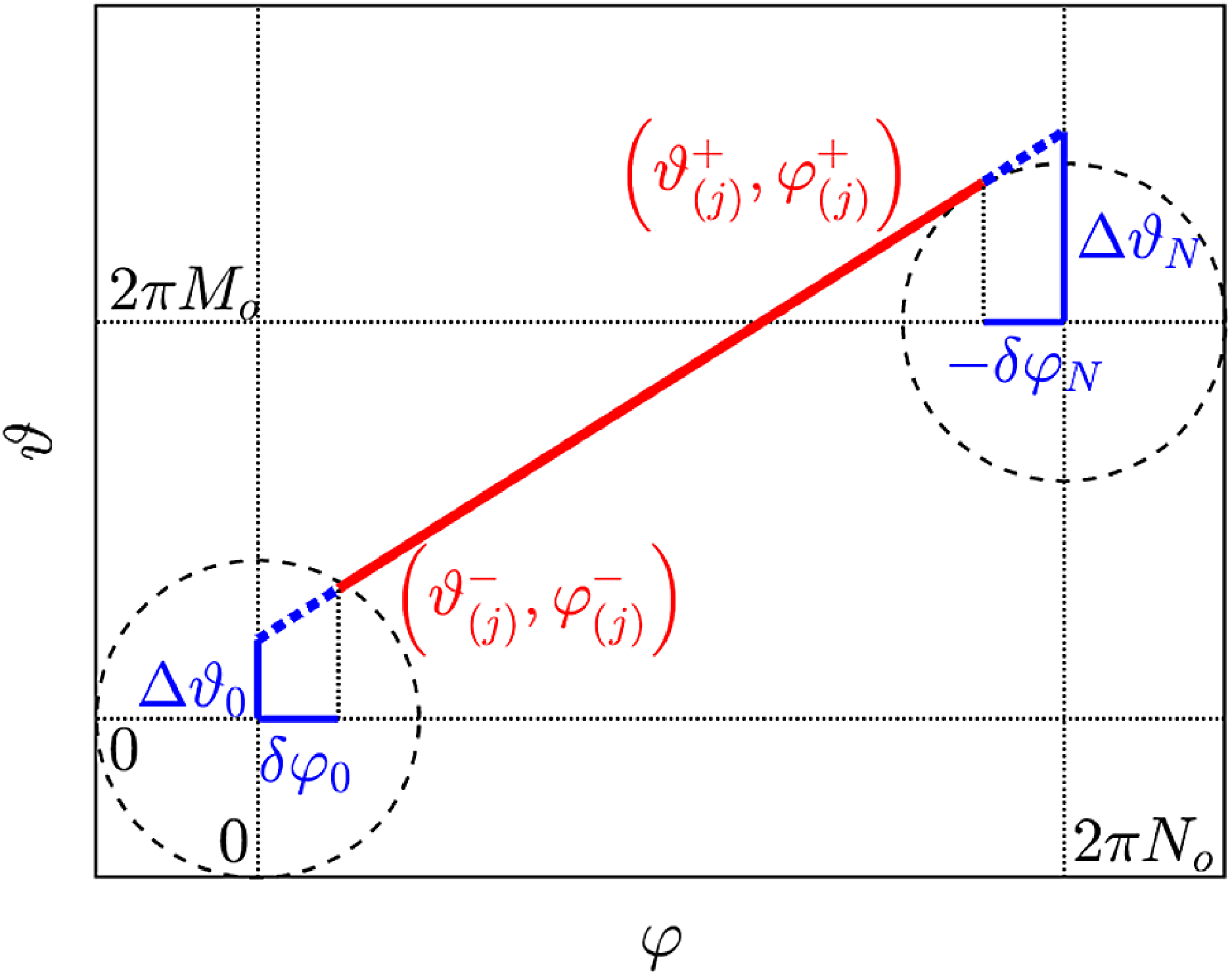
Figure 29. Field line segment containing the off-set domain (blue dotted) covered by transient banana orbit (red) in case the lower local field maximum is on the right, $\eta _{\textrm{loc}}^{(j)}=\eta _{j+1}$
. Dashed black ellipses correspond to the contour
$\eta _{\textrm{loc}}^{(j)}=\eta _{j+1}$
. Dashed black ellipses correspond to the contour $\eta _{\textrm{loc}}^{(j)} B(\vartheta, \varphi )=1$
.
$\eta _{\textrm{loc}}^{(j)} B(\vartheta, \varphi )=1$
.
 \begin{eqnarray} I_{\mathcal{V}}^{(j)}\; &\approx &\; \Delta \vartheta _{\text{mid}}\int \limits _{0}^{2\pi N_o}\textrm { d} \varphi \left ( \mathcal{V}_b^\prime (\iota _o \varphi, \varphi ) + \delta \iota \mathcal{V}_b^{\prime \prime }(\iota _o \varphi, \varphi ) (\varphi -\pi N_o) \right ) \nonumber \\ &=&\; 2\pi N_o\Delta \vartheta _{\text{mid}}\sum \limits _{m=1}^\infty \sum \limits _{n=-\infty }^\infty m\mathcal{V}_{mn}^s(\eta _b) \!\left (\!\delta _{\text{res}}+\frac {m N_o \delta \iota }{m M_o + n N_o}(1-\delta _{\text {res}}) \!\right )\!, \end{eqnarray}
where $\delta _{\text {res}}=1$
if
$\delta _{\text {res}}=1$
if $mM_o-nN_o=0$
and is zero otherwise, and
$mM_o-nN_o=0$
and is zero otherwise, and $\Delta \vartheta _{\text{mid}}=(\Delta \vartheta _0+\Delta \vartheta _N)/2$
. Since only the resonant harmonics with
$\Delta \vartheta _{\text{mid}}=(\Delta \vartheta _0+\Delta \vartheta _N)/2$
. Since only the resonant harmonics with $(m,n) = \left (N_o k,-M_o k\right )$
and
$(m,n) = \left (N_o k,-M_o k\right )$
and $k=1,2,\ldots$
contribute to the first term, one can estimate
$k=1,2,\ldots$
contribute to the first term, one can estimate $\sum \sum m \mathcal{V}_{mn}^s \delta _{\text{res}} \sim N_o \mathcal{V}_{N_o,-M_o}^s$
. For high harmonic indices,
$\sum \sum m \mathcal{V}_{mn}^s \delta _{\text{res}} \sim N_o \mathcal{V}_{N_o,-M_o}^s$
. For high harmonic indices, $m,n \rightarrow \infty$
, spectrum of
$m,n \rightarrow \infty$
, spectrum of $\mathcal{V}$
is determined by the vicinity of the global maximum,
$\mathcal{V}$
is determined by the vicinity of the global maximum,
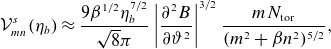 \begin{align} \mathcal{V}_{mn}^s(\eta _b) \approx \frac {9 \beta ^{1/2} \eta _b^{7/2}}{\sqrt {8} \pi } \left |\frac {\partial ^2 B}{\partial \vartheta ^2}\right |^{3/2} \frac {m N_{\text{tor}}}{(m^2 + \beta n^2)^{5/2}}, \end{align}
where $N_{\text{tor}}$
is the number of toroidal field periods and
$N_{\text{tor}}$
is the number of toroidal field periods and $\mathcal{V}_{mn}^s=0$
for
$\mathcal{V}_{mn}^s=0$
for $n$
which are not multiples of
$n$
which are not multiples of $N_{\text{tor}}$
, see Appendix A. Therefore, contribution of the first term
$N_{\text{tor}}$
, see Appendix A. Therefore, contribution of the first term $N_o \mathcal{V}_{N_o,-M_o}^s \sim N_o^{-3}$
is negligibly small compared with that of the second term which does not scale with
$N_o \mathcal{V}_{N_o,-M_o}^s \sim N_o^{-3}$
is negligibly small compared with that of the second term which does not scale with $N_o$
but contains small
$N_o$
but contains small $\delta \iota$
. Using
$\delta \iota$
. Using $2\pi N_o \delta \iota = \Delta \vartheta _N-\Delta \vartheta _0$
and the definition of
$2\pi N_o \delta \iota = \Delta \vartheta _N-\Delta \vartheta _0$
and the definition of $\Delta \vartheta _{\text {mid}}$
, we obtain the scaling
$\Delta \vartheta _{\text {mid}}$
, we obtain the scaling $I_{\mathcal{V}}^{(j)} \propto (\Delta \vartheta _N^2-\Delta \vartheta _0^2) \propto N_o^{-2} \propto N^{-2}$
and respective estimates
$I_{\mathcal{V}}^{(j)} \propto (\Delta \vartheta _N^2-\Delta \vartheta _0^2) \propto N_o^{-2} \propto N^{-2}$
and respective estimates
 \begin{align} w_{\text{off}}^{(j)} \sim \frac {\varepsilon _t^{3/2}}{N^3}\frac {\textrm { d} r}{\textrm { d} \psi } \sim \left (\varepsilon _t\nu _\ast \right )^{3/5}\frac {\textrm { d} r}{\textrm { d} \psi }, \qquad \lambda _{\text{off}}^{\textrm{max}} \sim \varepsilon _t^{1/2} R B_0 \frac {\textrm { d} r}{\textrm { d} \psi } \sim \iota \lambda _{bB}^{\text{tok}}, \end{align}
where we assumed the maximum distribution function off-set (4.7), used (4.6) and assumed $\varepsilon _M \sim \varepsilon _t$
and
$\varepsilon _M \sim \varepsilon _t$
and $\beta \sim 1$
. Thus, off-set of bootstrap coefficient
$\beta \sim 1$
. Thus, off-set of bootstrap coefficient $\lambda _{\text{off}}$
in stellarator-symmetric fields does not decrease with reducing collisionality but has an aperiodic oscillatory behavior with oscillation amplitude
$\lambda _{\text{off}}$
in stellarator-symmetric fields does not decrease with reducing collisionality but has an aperiodic oscillatory behavior with oscillation amplitude $\lambda _{\text{off}}^{\textrm{max}}$
of the order of
$\lambda _{\text{off}}^{\textrm{max}}$
of the order of $\lambda _{bB}$
for the equivalent tokamak (Boozer & Gardner Reference Boozer and Gardner1990; Beidler et al. Reference Beidler2011),
$\lambda _{bB}$
for the equivalent tokamak (Boozer & Gardner Reference Boozer and Gardner1990; Beidler et al. Reference Beidler2011),
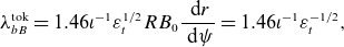 \begin{align} \lambda _{bB}^{\text{tok}} = 1.46 \iota ^{-1}\varepsilon _t^{1/2}RB_0 \frac {\textrm { d} r}{\textrm { d} \psi } = 1.46 \iota ^{-1}\varepsilon _t^{-1/2}, \end{align}
see figure 20 where the factor $1.46 \iota ^{-1} \approx 3.4$
agrees well with the relative off-set amplitude.
$1.46 \iota ^{-1} \approx 3.4$
agrees well with the relative off-set amplitude.
The off-set pattern corresponding to $N$
toroidal turns is replaced by the pattern with a larger number of turns if collisionality decreases by a significant factor, and further collisionality decrease triggers another pattern change, etc. Respectively, the off-set of the bootstrap coefficient oscillates aperiodically with changing
$N$
toroidal turns is replaced by the pattern with a larger number of turns if collisionality decreases by a significant factor, and further collisionality decrease triggers another pattern change, etc. Respectively, the off-set of the bootstrap coefficient oscillates aperiodically with changing $\log \nu _\ast$
as seen in figure 20. This behavior is due to the structure of the off-set pattern which is formed at the field line segment between two local field maxima
$\log \nu _\ast$
as seen in figure 20. This behavior is due to the structure of the off-set pattern which is formed at the field line segment between two local field maxima $j=0,N$
fulfilling strong alignment conditions
$j=0,N$
fulfilling strong alignment conditions $(\Delta \eta _0,\Delta \eta _N) \ll \delta \eta$
with
$(\Delta \eta _0,\Delta \eta _N) \ll \delta \eta$
with $\delta \eta$
given by (4.5) and which necessarily contains one or more internal local maxima fulfilling a weak alignment condition
$\delta \eta$
given by (4.5) and which necessarily contains one or more internal local maxima fulfilling a weak alignment condition $\Delta \eta \lesssim \delta \eta$
(they split the segment into off-set domains, e.g. two off-set domains and the main region in the simplest case). With decreasing collisionality, weakly aligned internal maxima become non-aligned,
$\Delta \eta \lesssim \delta \eta$
(they split the segment into off-set domains, e.g. two off-set domains and the main region in the simplest case). With decreasing collisionality, weakly aligned internal maxima become non-aligned, $\Delta \eta \gg \delta \eta$
, which makes the variation of the distribution function off-set
$\Delta \eta \gg \delta \eta$
, which makes the variation of the distribution function off-set $g_{\text{off}}$
within the segment and respective contribution of the given pattern to the off-set of
$g_{\text{off}}$
within the segment and respective contribution of the given pattern to the off-set of $\lambda _{bB}$
exponentially small. Consequently, the whole segment of the old pattern turns into a single off-set domain of the new, longer pattern limited at the ends by even better aligned local maxima such that they stay well aligned when one (or both) maxima at the ends of the former segment become only weakly aligned at some lower collisionality. The above transition is well seen in figures 25 and 26 where three complete off-set patterns at higher collisionality (left figure 25) turn into three off-set domains of a longer pattern at lower collisionality (left figure 26). Note that those domains contribute simultaneously to both off-sets,
$\lambda _{bB}$
exponentially small. Consequently, the whole segment of the old pattern turns into a single off-set domain of the new, longer pattern limited at the ends by even better aligned local maxima such that they stay well aligned when one (or both) maxima at the ends of the former segment become only weakly aligned at some lower collisionality. The above transition is well seen in figures 25 and 26 where three complete off-set patterns at higher collisionality (left figure 25) turn into three off-set domains of a longer pattern at lower collisionality (left figure 26). Note that those domains contribute simultaneously to both off-sets, $g_{\text{off}}^{\text{short}}$
and
$g_{\text{off}}^{\text{short}}$
and $g_{\text{off}}^{\text{long}}$
with the first one being dominant at higher and the second one at lower collisionality. A kink on the collisionality dependence of a summary function
$g_{\text{off}}^{\text{long}}$
with the first one being dominant at higher and the second one at lower collisionality. A kink on the collisionality dependence of a summary function $g_{\text{off}}^{\text{(sp)}}= \max (g_{\text{off}}^{\text{short}},g_{\text{off}}^{\text{long}})$
shown in figure 28 is at the transition point
$g_{\text{off}}^{\text{(sp)}}= \max (g_{\text{off}}^{\text{short}},g_{\text{off}}^{\text{long}})$
shown in figure 28 is at the transition point $\nu _\ast = 10^{-4}$
where
$\nu _\ast = 10^{-4}$
where $g_{\text{off}}^{\text{short}}=g_{\text{off}}^{\text{long}}$
. At this point, internal maxima of the long off-set domain are still well aligned, so that
$g_{\text{off}}^{\text{short}}=g_{\text{off}}^{\text{long}}$
. At this point, internal maxima of the long off-set domain are still well aligned, so that $g_{\text{off}}^{\text{long}}$
scaling with
$g_{\text{off}}^{\text{long}}$
scaling with $\nu _\ast$
is similar to (3.53) which includes
$\nu _\ast$
is similar to (3.53) which includes $1/\nu$
and
$1/\nu$
and $1/\sqrt {\nu }$
terms. Note that
$1/\sqrt {\nu }$
terms. Note that $g_{\text{off}}^{\text{(sp)}}$
in figure 28 by definition shows only the largest off-set within the pattern which generally contains more than two off-set domains (see figure 26). Therefore, location of
$g_{\text{off}}^{\text{(sp)}}$
in figure 28 by definition shows only the largest off-set within the pattern which generally contains more than two off-set domains (see figure 26). Therefore, location of $g_{\text{off}}^{\text{(sp)}}$
maximum at
$g_{\text{off}}^{\text{(sp)}}$
maximum at $\nu _\ast$
dependence needs not coincide with the location of respective
$\nu _\ast$
dependence needs not coincide with the location of respective $\lambda _{bB}$
maximum, which is at lower
$\lambda _{bB}$
maximum, which is at lower $\nu _\ast$
in figure 20. The reason is that contributions of most off-set domains within the pattern tend to saturate and then vanish with decreasing
$\nu _\ast$
in figure 20. The reason is that contributions of most off-set domains within the pattern tend to saturate and then vanish with decreasing $\nu _\ast$
earlier than
$\nu _\ast$
earlier than $g_{\text{off}}^{\text{(sp)}}$
which is determined then by the off-set domain bounded by the best aligned local maxima. One should also note that another kink on
$g_{\text{off}}^{\text{(sp)}}$
which is determined then by the off-set domain bounded by the best aligned local maxima. One should also note that another kink on $g_{\text{off}}^{\text{(sp)}}$
located in figure 28 at
$g_{\text{off}}^{\text{(sp)}}$
located in figure 28 at $\nu _\ast = 1.7\cdot 10^{-10}$
is not the transition point of different off-set patterns but a point where the off-set for the same pattern changes sign due to the mirroring within trapped-passing boundary layer discussed, in particular, in § 3.1. As a result, the respective off-set of
$\nu _\ast = 1.7\cdot 10^{-10}$
is not the transition point of different off-set patterns but a point where the off-set for the same pattern changes sign due to the mirroring within trapped-passing boundary layer discussed, in particular, in § 3.1. As a result, the respective off-set of $\lambda _{bB}$
in figure 20 changes sign too (similar to figure 2).
$\lambda _{bB}$
in figure 20 changes sign too (similar to figure 2).
According to (4.2), better alignment of maxima at the off-set segment ends means smaller poloidal displacements $\Delta \vartheta _0$
and
$\Delta \vartheta _0$
and $\Delta \vartheta _N$
of these ends, which requires a decrease with the pattern length
$\Delta \vartheta _N$
of these ends, which requires a decrease with the pattern length $N$
of the difference
$N$
of the difference $|\Delta \vartheta _N-\Delta \vartheta _0|=2\pi |\iota N_p -M|$
where
$|\Delta \vartheta _N-\Delta \vartheta _0|=2\pi |\iota N_p -M|$
where $N_p=N N_{\text{tor}}$
is the (integer) number of toroidal field periods within the off-set pattern and integer
$N_p=N N_{\text{tor}}$
is the (integer) number of toroidal field periods within the off-set pattern and integer $M$
is the nearest to
$M$
is the nearest to $\iota N_p$
. Thus, the increasing sequence of
$\iota N_p$
. Thus, the increasing sequence of $N_p$
corresponds to the sequence of the best Diophantine approximations
$N_p$
corresponds to the sequence of the best Diophantine approximations $M/N_p$
of (generally irrational)
$M/N_p$
of (generally irrational) $\iota$
. These approximations are the convergents of
$\iota$
. These approximations are the convergents of $\iota$
representation by a simple continued fraction (see, e.g., Hardy & Wright (Reference Hardy and Wright1985)). Therefore, an overall trend of the
$\iota$
representation by a simple continued fraction (see, e.g., Hardy & Wright (Reference Hardy and Wright1985)). Therefore, an overall trend of the $N_p$
series
$N_p$
series $N_p^{(k)}$
,
$N_p^{(k)}$
, $k=1,2,\ldots$
, is similar to that of geometrical progression,
$k=1,2,\ldots$
, is similar to that of geometrical progression, $N_{p}^{(k+1)}=b_k N_p^{(k)}$
with
$N_{p}^{(k+1)}=b_k N_p^{(k)}$
with $b_k \gt 1$
such that
$b_k \gt 1$
such that $b_k-1 \gtrsim 1$
. Thus, due to
$b_k-1 \gtrsim 1$
. Thus, due to $\nu _\ast \propto N_p^{-5}$
following from (4.6), a series of collisionalities
$\nu _\ast \propto N_p^{-5}$
following from (4.6), a series of collisionalities $\nu _\ast ^{(k)}$
corresponding to the dominance of pattern
$\nu _\ast ^{(k)}$
corresponding to the dominance of pattern $k$
in the off-set has similar geometrical trend, and a significant change in the off-set of
$k$
in the off-set has similar geometrical trend, and a significant change in the off-set of $\lambda _{bB}$
requires such a change of
$\lambda _{bB}$
requires such a change of $\log \nu _\ast$
.
$\log \nu _\ast$
.
Finally, in view of the off-set (4.12) being of the same order as the collisionless asymptotic (2.43), let us estimate the role of the correction term driven by the source (3.13) which has been ignored in the present analysis and estimated to have a vanishing effect with decreasing collisionality in a short field line example in § 3.4. Comparison of the asymptotic and numerical solutions in figure 25 shows an obvious feature which cannot be described by the leading-order off-set. Namely, instead of the continuous linear growth of $g_o^t$
, numerical solution tends to a nearly periodic behavior with the period of the order of the off-set pattern length. In other words, finite collisionality provides an aperiodic correction term which nearly balances the aperiodic behavior of
$g_o^t$
, numerical solution tends to a nearly periodic behavior with the period of the order of the off-set pattern length. In other words, finite collisionality provides an aperiodic correction term which nearly balances the aperiodic behavior of $g_0^t$
(while the leading-order off-set provides only a nearly periodic correction contained in the off-set domains within the pattern). One can formally present this next-order correction as a ‘staircase function’,
$g_0^t$
(while the leading-order off-set provides only a nearly periodic correction contained in the off-set domains within the pattern). One can formally present this next-order correction as a ‘staircase function’, $\Delta g_{\text{off}}^{\text{(tr)}}=\sum _k C_k^{\text{(tr)}} \Theta \left (\varphi -\varphi _k^{\text{(op)}}\right )$
, where
$\Delta g_{\text{off}}^{\text{(tr)}}=\sum _k C_k^{\text{(tr)}} \Theta \left (\varphi -\varphi _k^{\text{(op)}}\right )$
, where $\varphi _k^{\text {(op)}}$
are the boundaries of the off-set pattern (points of well aligned relevant maxima) and
$\varphi _k^{\text {(op)}}$
are the boundaries of the off-set pattern (points of well aligned relevant maxima) and $C_k^{\text{(tr)}}=g_0^t\left (\varphi _{k-1}^{\text{(op)}}\right )-g_0^t\left (\varphi _{k}^{\text{(op)}}\right )$
. Being of the same order as
$C_k^{\text{(tr)}}=g_0^t\left (\varphi _{k-1}^{\text{(op)}}\right )-g_0^t\left (\varphi _{k}^{\text{(op)}}\right )$
. Being of the same order as $g_0^t$
which, due to its dependence on
$g_0^t$
which, due to its dependence on $\varphi$
, makes an independent of collisionality contribution to
$\varphi$
, makes an independent of collisionality contribution to $\lambda _{bB}$
within each off-set pattern, the staircase function is constant within the pattern and, according to the first estimate (4.12), its contribution scales with collisionality. Namely, replacing the distribution function off-set
$\lambda _{bB}$
within each off-set pattern, the staircase function is constant within the pattern and, according to the first estimate (4.12), its contribution scales with collisionality. Namely, replacing the distribution function off-set $g_{\text{off}}^{(j)}$
with
$g_{\text{off}}^{(j)}$
with $\Delta g_{\text{off}}^{\text{(tr)}} \sim N N_{\text{pt}}$
where
$\Delta g_{\text{off}}^{\text{(tr)}} \sim N N_{\text{pt}}$
where $N_{\text{pt}}$
is the number of patterns per closed field line (and
$N_{\text{pt}}$
is the number of patterns per closed field line (and $N$
, as before, is the number of toroidal turns within the pattern), respective contribution to the bootstrap coefficient scales as
$N$
, as before, is the number of toroidal turns within the pattern), respective contribution to the bootstrap coefficient scales as $\Delta \lambda _{bB} \approx w_{\text{off}}^{(j)} \Delta g_{\text{off}}^{\text {(tr)}} \sim N_{\text{pt}} N^{-2} \sim N_{\text{pt}} \nu _\ast ^{2/5}$
.
$\Delta \lambda _{bB} \approx w_{\text{off}}^{(j)} \Delta g_{\text{off}}^{\text {(tr)}} \sim N_{\text{pt}} N^{-2} \sim N_{\text{pt}} \nu _\ast ^{2/5}$
.
Another feature demonstrated for the short field line in figure 8 is a split of the boundary layer caused by a strong alignment of relevant maxima. This split can also be formally described by a staircase function $\Delta g_{\text{off}}^{\text{(bl)}} =\sum _k C_k^{\text{(bl)}} \Theta \left (\varphi -\varphi _k^{\text{(op)}}\right )\delta _{\text{(b)}}(\eta _b-\eta )$
where
$\Delta g_{\text{off}}^{\text{(bl)}} =\sum _k C_k^{\text{(bl)}} \Theta \left (\varphi -\varphi _k^{\text{(op)}}\right )\delta _{\text{(b)}}(\eta _b-\eta )$
where $\delta _{\text {(b)}}$
tends with vanishing collisionality to a
$\delta _{\text {(b)}}$
tends with vanishing collisionality to a $\delta$
-function and is localized within the boundary layer width
$\delta$
-function and is localized within the boundary layer width $\delta \eta$
where it scales as
$\delta \eta$
where it scales as $\delta \eta ^{-1}$
at finite collisionality, whereas constants
$\delta \eta ^{-1}$
at finite collisionality, whereas constants $C_k^{\text{(bl)}}$
are given by the integral in parentheses in (2.52) with the change of lower and upper limits to
$C_k^{\text{(bl)}}$
are given by the integral in parentheses in (2.52) with the change of lower and upper limits to $\varphi _k^{\text {(op)}}$
and
$\varphi _k^{\text {(op)}}$
and $\varphi _{k-1}^{\text {(op)}}$
, respectively. Since
$\varphi _{k-1}^{\text {(op)}}$
, respectively. Since $\Delta g_{\text{off}}^{\text{(bl)}}$
is also a constant of
$\Delta g_{\text{off}}^{\text{(bl)}}$
is also a constant of $\varphi$
within the pattern, its contribution to
$\varphi$
within the pattern, its contribution to $\lambda _{bB}$
can be estimated as
$\lambda _{bB}$
can be estimated as $\Delta \lambda _{bB} \sim \Delta w_{\text{off}}^{(j)}\Delta g_{\text{off}}^{\text{(bl)}}$
where
$\Delta \lambda _{bB} \sim \Delta w_{\text{off}}^{(j)}\Delta g_{\text{off}}^{\text{(bl)}}$
where $\Delta g_{\text{off}}^{\text {(bl)}} \sim N N_{\text{pt}} \delta \eta ^{-1}$
, and the estimate
$\Delta g_{\text{off}}^{\text {(bl)}} \sim N N_{\text{pt}} \delta \eta ^{-1}$
, and the estimate $\Delta w_{\text{off}}^{(j)} \sim N^{-1} \Delta I_\mathcal{V}^{(j)}$
follows from (3.59), where
$\Delta w_{\text{off}}^{(j)} \sim N^{-1} \Delta I_\mathcal{V}^{(j)}$
follows from (3.59), where $\Delta I_\mathcal{V}^{(j)} \sim \delta \vartheta ^3 \sim N^{-3}$
is the contribution of the boundary layer to the integral
$\Delta I_\mathcal{V}^{(j)} \sim \delta \vartheta ^3 \sim N^{-3}$
is the contribution of the boundary layer to the integral $I_\mathcal{V}^{(j)}$
(this estimate is similar to the estimate of the error due to the finite
$I_\mathcal{V}^{(j)}$
(this estimate is similar to the estimate of the error due to the finite $\eta _{\textrm{loc}}^{(j)}-\eta _b$
below (4.9)). Finally, we obtain
$\eta _{\textrm{loc}}^{(j)}-\eta _b$
below (4.9)). Finally, we obtain $\Delta \lambda _{bB} \sim N_{\text{pt}}N^{-3} \delta \eta ^{-1}\sim N_{\text{pt}}N^{-1} \sim N_{\text{pt}} \nu _\ast ^{1/5}$
where we used (4.6) treated again as an approximate equality instead of a strong inequality. Thus, despite a visible effect on the generalized Spitzer function
$\Delta \lambda _{bB} \sim N_{\text{pt}}N^{-3} \delta \eta ^{-1}\sim N_{\text{pt}}N^{-1} \sim N_{\text{pt}} \nu _\ast ^{1/5}$
where we used (4.6) treated again as an approximate equality instead of a strong inequality. Thus, despite a visible effect on the generalized Spitzer function $g_{(3)}$
, the ignored correction provides to the bootstrap coefficient a contribution which is converging to zero with decreasing collisionality.
$g_{(3)}$
, the ignored correction provides to the bootstrap coefficient a contribution which is converging to zero with decreasing collisionality.
It should be noted that scaling $\Delta \lambda _{bB} \propto N_{\text{pt}}$
with the number of off-set patterns within the closed field line is the result of the ‘worst case’ estimate allowing for ‘bootstrap resonances’ discussed below in § 4.4. Such a crude ‘worst case’ estimate of the collisionless asymptotic
$\Delta \lambda _{bB} \propto N_{\text{pt}}$
with the number of off-set patterns within the closed field line is the result of the ‘worst case’ estimate allowing for ‘bootstrap resonances’ discussed below in § 4.4. Such a crude ‘worst case’ estimate of the collisionless asymptotic $\lambda _{bB}^\dagger$
in the form (2.56) results in a similar scaling with the field line length which, in turn, does not contain the collisionality dependence.
$\lambda _{bB}^\dagger$
in the form (2.56) results in a similar scaling with the field line length which, in turn, does not contain the collisionality dependence.
4.3. Off-set of bootstrap/Ware-pinch coefficient in case of (nearly) aligned maxima
In the advanced stellarator configurations aiming at good confinement of fusion alpha particles, global magnetic field maxima tend to be aligned. This is the case in ideal quasi-symmetric configurations (Nührenberg & Zille, Reference Nührenberg and Zille1988) and also in quasi-isodynamic configurations with poloidally closed contours $B=\textrm{const}$
(Mikhailov et al. Reference Mikhailov, Shafranov, Subbotin, Isaev, Nührenberg, Zille and Cooper2002; Subbotin et al. Reference Subbotin2006). If these configurations are not realized exactly, poloidal (helical in the general case of quasi-symmetry) closure of
$B=\textrm{const}$
(Mikhailov et al. Reference Mikhailov, Shafranov, Subbotin, Isaev, Nührenberg, Zille and Cooper2002; Subbotin et al. Reference Subbotin2006). If these configurations are not realized exactly, poloidal (helical in the general case of quasi-symmetry) closure of $B=\textrm{const.}$
contours is destroyed, in particular, near the field maximum where these contours split into islands centered around the global maxima reached at one or few points instead of lines. Local maxima
$B=\textrm{const.}$
contours is destroyed, in particular, near the field maximum where these contours split into islands centered around the global maxima reached at one or few points instead of lines. Local maxima $\textbf {h}\cdot \nabla B=0$
, nevertheless, stay on poloidally closed contours defined in periodic Boozer coordinates by
$\textbf {h}\cdot \nabla B=0$
, nevertheless, stay on poloidally closed contours defined in periodic Boozer coordinates by $\varphi =\varphi _k^{\textrm{loc}}(\vartheta )$
where
$\varphi =\varphi _k^{\textrm{loc}}(\vartheta )$
where $\varphi _k^{\textrm{loc}}(\vartheta ) =\varphi _0^{\textrm{loc}}(\vartheta )+2\pi k/N_{\text{tor}}$
with
$\varphi _k^{\textrm{loc}}(\vartheta ) =\varphi _0^{\textrm{loc}}(\vartheta )+2\pi k/N_{\text{tor}}$
with $k$
being an integer, and where
$k$
being an integer, and where $\varphi _0^{\textrm{loc}}(\vartheta )$
is periodic. For simplicity, we restrict our analysis here to the case of poloidally closed contours where also the family of anti-sigma configurations (3.36) belongs as a sub-class with
$\varphi _0^{\textrm{loc}}(\vartheta )$
is periodic. For simplicity, we restrict our analysis here to the case of poloidally closed contours where also the family of anti-sigma configurations (3.36) belongs as a sub-class with $\varphi _0^{\textrm{loc}}(\vartheta )=0$
. We assume that these local maxima are close to global such that perturbation
$\varphi _0^{\textrm{loc}}(\vartheta )=0$
. We assume that these local maxima are close to global such that perturbation $\Delta B_{\textrm{loc}}(\vartheta ) \equiv B(\vartheta, \varphi _0^{\textrm{loc}}(\vartheta ))-\bar B_{\textrm{max}}$
of the global maximum
$\Delta B_{\textrm{loc}}(\vartheta ) \equiv B(\vartheta, \varphi _0^{\textrm{loc}}(\vartheta ))-\bar B_{\textrm{max}}$
of the global maximum $\bar B_{\textrm{max}}$
achieved in the ideal (unperturbed) configuration on a line is small. Since
$\bar B_{\textrm{max}}$
achieved in the ideal (unperturbed) configuration on a line is small. Since $(\vartheta, \varphi )=(0,0)$
is a stellarator symmetry point associated with field maximum, function
$(\vartheta, \varphi )=(0,0)$
is a stellarator symmetry point associated with field maximum, function $\varphi _0^{\textrm{loc}}(\vartheta )$
is odd and
$\varphi _0^{\textrm{loc}}(\vartheta )$
is odd and $\Delta B(\vartheta )$
is even.
$\Delta B(\vartheta )$
is even.
It is convenient now to label the field lines by the poloidal angle in the middle of the first field period where $\varphi =\varphi _s\equiv \pi /N_{\text{tor}}$
such that
$\varphi =\varphi _s\equiv \pi /N_{\text{tor}}$
such that $(\vartheta, \varphi )=(0,\varphi _s)$
is a stellarator symmetry point associated with field minimum of the ideal configuration. Namely, we label them with
$(\vartheta, \varphi )=(0,\varphi _s)$
is a stellarator symmetry point associated with field minimum of the ideal configuration. Namely, we label them with $\vartheta _0 = \vartheta -\iota (\varphi -\varphi _s)=\vartheta -\iota \varphi +\iota _p$
where
$\vartheta _0 = \vartheta -\iota (\varphi -\varphi _s)=\vartheta -\iota \varphi +\iota _p$
where $\iota _p=\iota \varphi _s$
. Positions of local maxima on the so labeled field line,
$\iota _p=\iota \varphi _s$
. Positions of local maxima on the so labeled field line, $\varphi _k=\varphi _k(\vartheta _0)$
, being the solutions to
$\varphi _k=\varphi _k(\vartheta _0)$
, being the solutions to $\varphi _k = \varphi _k^{\textrm{loc}}\left (\vartheta _0+\iota (\varphi _k-\varphi _s)\right )$
for
$\varphi _k = \varphi _k^{\textrm{loc}}\left (\vartheta _0+\iota (\varphi _k-\varphi _s)\right )$
for $-\infty \lt k \lt \infty$
can all be expressed via the left maximum of the first period
$-\infty \lt k \lt \infty$
can all be expressed via the left maximum of the first period $\varphi _0$
on the re-labeled field line as
$\varphi _0$
on the re-labeled field line as $\varphi _k(\vartheta _0) = \varphi _0\left (\vartheta _0 + 2 k \iota _p\right )+2 k\varphi _s$
. Respective perturbations
$\varphi _k(\vartheta _0) = \varphi _0\left (\vartheta _0 + 2 k \iota _p\right )+2 k\varphi _s$
. Respective perturbations $\Delta B_{(k)}(\vartheta _0)$
of global maximum at these points can be expressed via such perturbation
$\Delta B_{(k)}(\vartheta _0)$
of global maximum at these points can be expressed via such perturbation $\Delta B_{(0)}$
of the left maximum in the first period as
$\Delta B_{(0)}$
of the left maximum in the first period as $\Delta B_{(k)}(\vartheta _0) = \Delta B_{(0)}(\vartheta _0+2k\iota _p)$
. Finally, integrals (2.26) where
$\Delta B_{(k)}(\vartheta _0) = \Delta B_{(0)}(\vartheta _0+2k\iota _p)$
. Finally, integrals (2.26) where $\varphi _j^-=\varphi _j$
and
$\varphi _j^-=\varphi _j$
and $\varphi _j^+=\varphi _{j+1}$
can be mapped to the first period similarly,
$\varphi _j^+=\varphi _{j+1}$
can be mapped to the first period similarly, $I_k(\vartheta _0,\eta ) = I_0(\vartheta _0+2k\iota _p,\eta )$
.
$I_k(\vartheta _0,\eta ) = I_0(\vartheta _0+2k\iota _p,\eta )$
.
Due to stellarator symmetry, function $\varphi _0(\vartheta _0)$
is odd with respect to
$\varphi _0(\vartheta _0)$
is odd with respect to $\vartheta _0-\iota _p$
, i.e.
$\vartheta _0-\iota _p$
, i.e. $\varphi _0(2\iota _p-\vartheta _0)=-\varphi _0(\vartheta _0)$
, while function
$\varphi _0(2\iota _p-\vartheta _0)=-\varphi _0(\vartheta _0)$
, while function $\Delta B_{(0)}$
is even. It convenient to express the latter via an even function of the argument
$\Delta B_{(0)}$
is even. It convenient to express the latter via an even function of the argument $\Delta B(\vartheta ^\prime )$
as
$\Delta B(\vartheta ^\prime )$
as $\Delta B_{(0)}(\vartheta _0)=\Delta B(\vartheta _0-\iota _p)$
, such that for anti-sigma configurations we have an identity
$\Delta B_{(0)}(\vartheta _0)=\Delta B(\vartheta _0-\iota _p)$
, such that for anti-sigma configurations we have an identity $\Delta B(\vartheta )=\Delta B_{\textrm{loc}}(\vartheta ) = B(\vartheta, 0)-\bar B_{\textrm{max}}$
. We fix
$\Delta B(\vartheta )=\Delta B_{\textrm{loc}}(\vartheta ) = B(\vartheta, 0)-\bar B_{\textrm{max}}$
. We fix $\bar B_{\textrm{max}}$
by the condition of zero average,
$\bar B_{\textrm{max}}$
by the condition of zero average, $\overline {\Delta B}=0$
such that an even function
$\overline {\Delta B}=0$
such that an even function $\Delta \eta (\vartheta )=-\Delta B(\vartheta )/\bar B_{\textrm{max}}^2$
has zero average too. Using definition (3.30) of the aspect ratio, its perturbation is given by
$\Delta \eta (\vartheta )=-\Delta B(\vartheta )/\bar B_{\textrm{max}}^2$
has zero average too. Using definition (3.30) of the aspect ratio, its perturbation is given by $\Delta A_o(\vartheta _0) = \left (I_{\text {ref}}/I_0(\vartheta _0,\eta _b)\right )^{1/2}-1$
being an even function with
$\Delta A_o(\vartheta _0) = \left (I_{\text {ref}}/I_0(\vartheta _0,\eta _b)\right )^{1/2}-1$
being an even function with $I_{\text{ref}}$
determined by the condition of zero average
$I_{\text{ref}}$
determined by the condition of zero average $\overline {\Delta A_o}$
.
$\overline {\Delta A_o}$
.
Mapping to the first period of the distribution function off-set given by (3.53) for small $\Delta A_o \ll 1$
and
$\Delta A_o \ll 1$
and $\Delta \eta \ll \delta \eta _{\text{ref}}$
is similar to that of the other quantities,
$\Delta \eta \ll \delta \eta _{\text{ref}}$
is similar to that of the other quantities, $g_{\text{off}}^{(0)}(\vartheta _0)=g_{\text{off}}^{(k)}(\vartheta _0-2k\iota _p)$
. Since (3.53) gives the off-set in open-ended system with sources located in a single period, solution for the closed (periodic) system with sources in each period is an odd function given by the sum over all periods of the open ended system
$g_{\text{off}}^{(0)}(\vartheta _0)=g_{\text{off}}^{(k)}(\vartheta _0-2k\iota _p)$
. Since (3.53) gives the off-set in open-ended system with sources located in a single period, solution for the closed (periodic) system with sources in each period is an odd function given by the sum over all periods of the open ended system
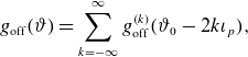 \begin{align} g_{\text{off}}(\vartheta ) = \sum \limits _{k=-\infty }^\infty g_{\text{off}}^{(k)}(\vartheta _0-2k\iota _p), \end{align}
which is expressed via even functions $\Delta A_o$
and
$\Delta A_o$
and $\Delta \eta$
as
$\Delta \eta$
as
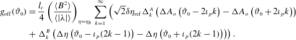 \begin{eqnarray} g_{\text{off}}(\vartheta _0) \;&=&\; \frac {l_c}{4}\left (\frac {\langle B^2\rangle }{\langle |\lambda |\rangle }\right )_{\eta =\eta _b} \sum \limits _{k=1}^\infty \left ( \sqrt {2} \delta \eta _{\text{ref}} \Delta ^A_k \left ( \Delta A_o\left (\vartheta _0-2\iota _p k \right ) -\Delta A_o\left (\vartheta _0+2\iota _p k \right ) \right ) \right . \nonumber \\ &+&\; \left . \Delta ^B_k \left ( \Delta \eta \left (\vartheta _0-\iota _p(2k-1) \right ) - \Delta \eta \left (\vartheta _0+\iota _p(2k-1) \right ) \right ) \right ). \end{eqnarray}
Respectively, the off-set of the Ware-pinch coefficient (3.54) is expressed in the limit of infinite (irrational) field-line length via $g_{\text {off}}$
as follows:
$g_{\text {off}}$
as follows:
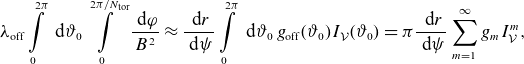 \begin{align} \lambda _{\text{off}} \int \limits _{0}^{2\pi }\textrm { d} \vartheta _0 \int \limits _{0}^{2\pi /N_{\text{tor}}}\frac {\textrm { d} \varphi }{B^2} \approx \frac {\textrm { d} r}{\textrm { d} \psi } \int \limits _{0}^{2\pi }\textrm { d} \vartheta _0\; g_{\text{off}}(\vartheta _0) I_\mathcal{V}(\vartheta _0) = \pi \frac {\textrm { d} r}{\textrm { d} \psi } \sum \limits _{m=1}^\infty g_m I_\mathcal{V}^m, \end{align}
where an odd function $I_\mathcal{V}(\vartheta _0)$
is given by the second (3.59) with
$I_\mathcal{V}(\vartheta _0)$
is given by the second (3.59) with $\varphi _{(j)}^-=\varphi _0(\vartheta _0)$
and
$\varphi _{(j)}^-=\varphi _0(\vartheta _0)$
and $\varphi _{(j)}^+=\varphi _1(\vartheta _0)$
, and we used (an odd) Fourier series expansion
$\varphi _{(j)}^+=\varphi _1(\vartheta _0)$
, and we used (an odd) Fourier series expansion
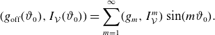 \begin{align} (g_{\text{off}}(\vartheta _0),I_\mathcal{V}(\vartheta _0)) = \sum \limits _{m=1}^\infty (g_m, I_\mathcal{V}^m)\sin (m\vartheta _0). \end{align}
Coefficients $g_m$
are expressed via coefficients of (an even) Fourier series expansion
$g_m$
are expressed via coefficients of (an even) Fourier series expansion
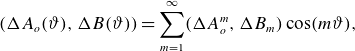 \begin{align} (\Delta A_o(\vartheta ), \Delta B(\vartheta )) = \sum \limits _{m=1}^\infty (\Delta A_o^m, \Delta B_m)\cos (m\vartheta ), \end{align}
as follows:
 \begin{align} g_m = \frac {l_c}{2}\left (\frac {\langle B^2\rangle }{\langle |\lambda |\rangle }\right )_{\!\!\eta =\eta _b} \left ( \sqrt {2} \delta \eta _{\text{ref}} S_A(m \iota _p) \Delta A_o^m - \eta _b^2 S_B(m \iota _p) \Delta B_m \right ), \end{align}
where
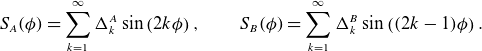 \begin{align} S_A(\phi ) = \sum \limits _{k=1}^\infty \Delta ^A_k \sin \left (2k\phi \right ), \qquad S_B(\phi ) = \sum \limits _{k=1}^\infty \Delta ^B_k \sin \left ((2k-1)\phi \right ). \end{align}
These functions have period $2\pi$
and are well approximated in the interval
$2\pi$
and are well approximated in the interval $-\pi \lt \phi \lt \pi$
by
$-\pi \lt \phi \lt \pi$
by $S_A(\phi ) \approx 0.26\, (\phi -(\pi /2)\text {sign}(\phi ))$
and
$S_A(\phi ) \approx 0.26\, (\phi -(\pi /2)\text {sign}(\phi ))$
and $S_B(\phi ) \approx 1.85\,\text {sign}(\phi )$
.
$S_B(\phi ) \approx 1.85\,\text {sign}(\phi )$
.
For the estimates, we apply general expressions (4.15)–(4.19) to the anti-sigma configuration (3.36) which corresponds to the perturbed case 3 with $\varepsilon _0=\varepsilon _M \ll 1$
,
$\varepsilon _0=\varepsilon _M \ll 1$
, $\varepsilon _1=\varepsilon _t \ll \varepsilon _M$
and
$\varepsilon _1=\varepsilon _t \ll \varepsilon _M$
and $\varepsilon _3=0$
 \begin{align} B(\vartheta, \varphi ) = B_0 \left ( 1{\kern-.5pt}+{\kern-.5pt}\varepsilon _M \cos (N_{\text{tor}}\varphi ) {\kern-.5pt}+{\kern-.5pt}\varepsilon _t \cos \vartheta \left (1{\kern-.5pt}-{\kern-.5pt} \cos (N_{\text{tor}}\varphi )\right ) \right ){\kern-.5pt}+{\kern-.5pt}\Delta B_1 \cos \vartheta . \end{align}
In the leading order over $\varepsilon _t/\varepsilon _M$
and
$\varepsilon _t/\varepsilon _M$
and $\Delta B_1/B_0$
, only
$\Delta B_1/B_0$
, only $A_o^1 \approx \varepsilon _t/(2 \varepsilon _M)$
harmonic and
$A_o^1 \approx \varepsilon _t/(2 \varepsilon _M)$
harmonic and $\Delta B_1$
harmonic contribute to
$\Delta B_1$
harmonic contribute to $\lambda _{\text{off}}$
because of the dominance in the
$\lambda _{\text{off}}$
because of the dominance in the $I_\mathcal{V}$
spectrum of harmonic
$I_\mathcal{V}$
spectrum of harmonic $I_\mathcal{V}^1 \approx - 8\varepsilon _t (2\varepsilon _M)^{1/2} (B_0^2 N_{\text{tor}})^{-1}$
. Estimating
$I_\mathcal{V}^1 \approx - 8\varepsilon _t (2\varepsilon _M)^{1/2} (B_0^2 N_{\text{tor}})^{-1}$
. Estimating $l_c=\pi R/(2\nu _\ast )$
,
$l_c=\pi R/(2\nu _\ast )$
, $\langle B^2 \rangle \approx B_0^2$
,
$\langle B^2 \rangle \approx B_0^2$
, $\eta _b \approx 1/B_0$
,
$\eta _b \approx 1/B_0$
, $\langle |\lambda | \rangle _{\eta =\eta _b} \approx \pi ^{-1}(8 \varepsilon _M)^{1/2}$
and
$\langle |\lambda | \rangle _{\eta =\eta _b} \approx \pi ^{-1}(8 \varepsilon _M)^{1/2}$
and $\delta \eta _{\text{ref}} \sim 4 \pi ^{-1/2} (2\varepsilon _M)^{1/4} (\nu _\ast /N_{\text{tor}})^{1/2}B_0^{-1}$
we get
$\delta \eta _{\text{ref}} \sim 4 \pi ^{-1/2} (2\varepsilon _M)^{1/4} (\nu _\ast /N_{\text{tor}})^{1/2}B_0^{-1}$
we get
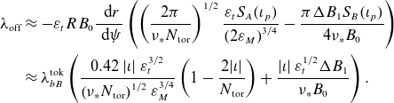 \begin{eqnarray} \lambda _{\text{off}} \;&\approx &\; -\varepsilon _t R B_0 \frac {\textrm { d} r}{\textrm { d} \psi } \left ( \left (\frac {2\pi }{\nu _\ast N_{\text{tor}}}\right )^{1/2} \frac {\varepsilon _t S_A(\iota _p) }{\left (2\varepsilon _M\right )^{3/4}} - \frac {\pi \Delta B_1 S_B(\iota _p)}{4\nu _\ast B_0} \right ) \nonumber \\ &\approx &\; \lambda _{bB}^{\text{tok}} \left ( \frac {0.42\;|\iota |\; \varepsilon _t^{3/2}}{\left (\nu _\ast N_{\text{tor}}\right )^{1/2}\varepsilon _M^{3/4}} \left (1-\frac {2|\iota |}{ N_{\text{tor}}}\right ) + \frac {|\iota |\;\varepsilon _t^{1/2} \Delta B_1}{\nu _\ast B_0} \right ). \end{eqnarray}
The black dotted line showing the trend in figure 14 actually corresponds to the result of this formula for case 3.
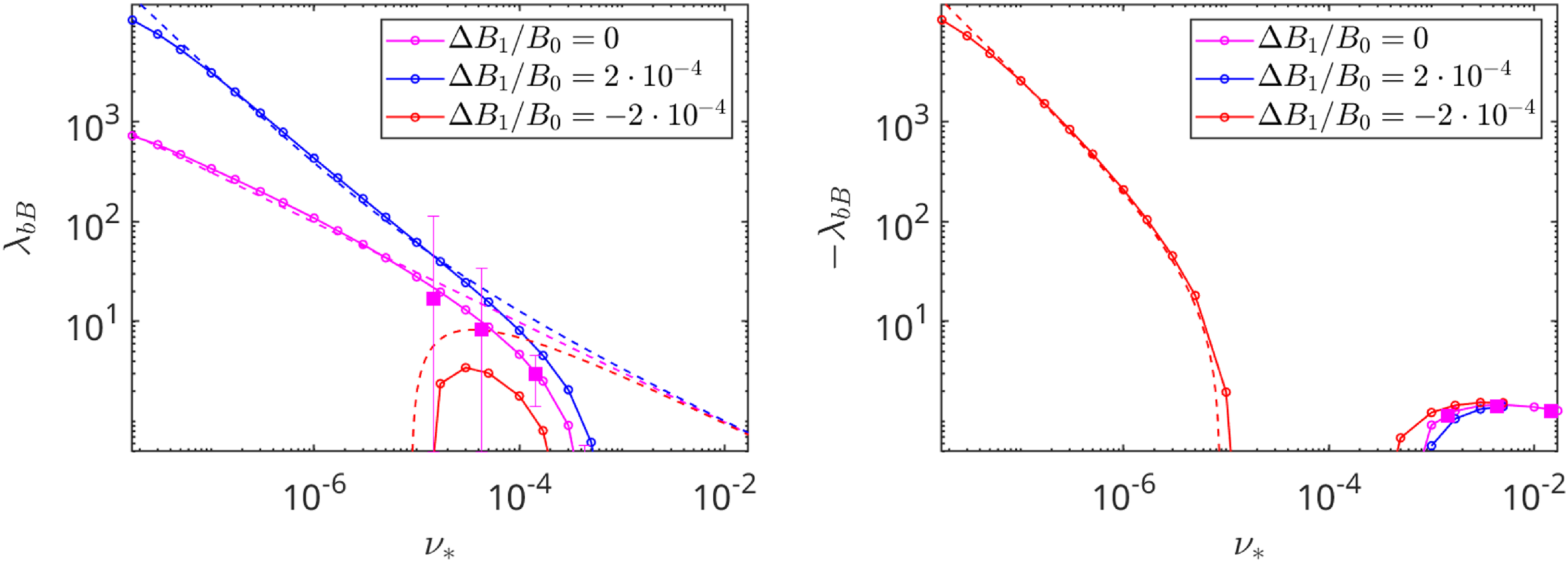
Figure 30. Geometrical factor $\lambda _{bB}$
computed by NEO-2 (circles) and DKES (filled squares) vs
$\lambda _{bB}$
computed by NEO-2 (circles) and DKES (filled squares) vs $\nu _\ast$
. Three different maximum-
$\nu _\ast$
. Three different maximum- $B$
perturbations are marked with colors (see the legend). Dashed lines correspond to the asymptotic (4.22). Negative
$B$
perturbations are marked with colors (see the legend). Dashed lines correspond to the asymptotic (4.22). Negative $\lambda _{bB}$
are shown in the right plot.
$\lambda _{bB}$
are shown in the right plot.
It should be reminded here that the off-set (4.22) due to violation of ripple equivalence appears only for relatively strong alignment of maxima, $\Delta B /B_0\lesssim (\nu_\ast / N_{\text{tor}})^{1/2} \varepsilon_M^{1/4}$
, and the validity of estimate (4.22) requires the respective strong inequality. In the marginal case where an approximate equality is realized, the largest off-set,
$\Delta B /B_0\lesssim (\nu_\ast / N_{\text{tor}})^{1/2} \varepsilon_M^{1/4}$
, and the validity of estimate (4.22) requires the respective strong inequality. In the marginal case where an approximate equality is realized, the largest off-set, $\lambda _{\text{off}} \sim \lambda _{bB}^{\text{tok}}\; \varepsilon _t^{1/2} \varepsilon _M^{1/4} \left (\nu _\ast N_{\text{tor}}\right )^{-1/2}$
occurs. The result of a small mis-alignment of maxima due to a finite perturbation
$\lambda _{\text{off}} \sim \lambda _{bB}^{\text{tok}}\; \varepsilon _t^{1/2} \varepsilon _M^{1/4} \left (\nu _\ast N_{\text{tor}}\right )^{-1/2}$
occurs. The result of a small mis-alignment of maxima due to a finite perturbation $\Delta B_1$
in (4.21) is shown in figure 30. Note that the validity condition of a linear asymptotic (4.22) becomes violated for finite
$\Delta B_1$
in (4.21) is shown in figure 30. Note that the validity condition of a linear asymptotic (4.22) becomes violated for finite $\Delta B_1$
at
$\Delta B_1$
at $\nu _\ast = 1.7\cdot 10^{-8}$
where
$\nu _\ast = 1.7\cdot 10^{-8}$
where $\Delta \eta = \delta \eta _{\text{ref}}$
, and the case of nearly aligned maxima starts a transition to the usual case of a global maximum reached at a point.
$\Delta \eta = \delta \eta _{\text{ref}}$
, and the case of nearly aligned maxima starts a transition to the usual case of a global maximum reached at a point.
4.4. Bootstrap resonances
As one can conclude from figure 20, resonance structure of $\iota$
(equivalently, of radial) dependence of bootstrap coefficient is absent in finite collisionality cases (see also figure 16 of Landreman et al. Reference Landreman, Buller and Drevlak2022). This, however, does not mean that these resonances never play a role. The reason for them is the following (see also the Appendix of Boozer & Gardner Reference Boozer and Gardner1990). By our assumption, the magnetic configuration has embedded flux surfaces everywhere so that magnetic islands are absent at any rational magnetic surface, which is manifested by a true surface condition (2.41). Although these configurations constitute a set of measure zero, they are physically possible. It is straightforward to check that the first term (representing the Pfirsch–Schlüter current) in (2.43) is never resonant as long as conditions (2.41) are fulfilled. However, this is not the case for the second term. Up to a flux surface function, the sub-integrand of the field line integral there is the derivative over
$\iota$
(equivalently, of radial) dependence of bootstrap coefficient is absent in finite collisionality cases (see also figure 16 of Landreman et al. Reference Landreman, Buller and Drevlak2022). This, however, does not mean that these resonances never play a role. The reason for them is the following (see also the Appendix of Boozer & Gardner Reference Boozer and Gardner1990). By our assumption, the magnetic configuration has embedded flux surfaces everywhere so that magnetic islands are absent at any rational magnetic surface, which is manifested by a true surface condition (2.41). Although these configurations constitute a set of measure zero, they are physically possible. It is straightforward to check that the first term (representing the Pfirsch–Schlüter current) in (2.43) is never resonant as long as conditions (2.41) are fulfilled. However, this is not the case for the second term. Up to a flux surface function, the sub-integrand of the field line integral there is the derivative over $\eta$
of the source term
$\eta$
of the source term $s_{(1)}$
, (2.3), which fulfills the quasi-Liouville theorem (2.15) at our representative field line, but not necessarily on the other field lines from the same rational surface. In other words, the amplitudes of resonant harmonics fulfilling
$s_{(1)}$
, (2.3), which fulfills the quasi-Liouville theorem (2.15) at our representative field line, but not necessarily on the other field lines from the same rational surface. In other words, the amplitudes of resonant harmonics fulfilling $\iota m + n = 0$
for our rational surface are generally finite, but these are harmonics of
$\iota m + n = 0$
for our rational surface are generally finite, but these are harmonics of $\sin (m\vartheta +n\varphi )=\sin (m\vartheta _0 + n\varphi _0 +(\iota m + n)(\varphi -\varphi _0))$
which are identical zeros for the starting point
$\sin (m\vartheta +n\varphi )=\sin (m\vartheta _0 + n\varphi _0 +(\iota m + n)(\varphi -\varphi _0))$
which are identical zeros for the starting point $(\vartheta _0,\varphi _0)$
being a stellarator symmetry point. Would those amplitudes be all zero, the integral over any field line would be a single-valued function fulfilling then a quasi-Liouville theorem (2.15) for passing particles and, as a consequence, conditions
$(\vartheta _0,\varphi _0)$
being a stellarator symmetry point. Would those amplitudes be all zero, the integral over any field line would be a single-valued function fulfilling then a quasi-Liouville theorem (2.15) for passing particles and, as a consequence, conditions $\oint \textrm {d} l\, v_\parallel = \text {const}$
evaluated for passing particles along closed field lines (see the discussion by Shaing & Callen (Reference Shaing and Callen1983) after equation (44b)), which actually mean ‘true surface’ conditions for the effective magnetic field
$\oint \textrm {d} l\, v_\parallel = \text {const}$
evaluated for passing particles along closed field lines (see the discussion by Shaing & Callen (Reference Shaing and Callen1983) after equation (44b)), which actually mean ‘true surface’ conditions for the effective magnetic field ${\textbf {B}}^\ast$
(Morozov & Solov’ev Reference Morozov and Solov’ev1966), i.e. for drift surfaces. The latter, however, need not have the same topology as the magnetic surfaces (see, e.g. Heyn et al. Reference Heyn, Ivanov, Kasilov, Kernbichler, Loarte, Nemov and Runov2012) and, at best, can be made embedded for one particular
${\textbf {B}}^\ast$
(Morozov & Solov’ev Reference Morozov and Solov’ev1966), i.e. for drift surfaces. The latter, however, need not have the same topology as the magnetic surfaces (see, e.g. Heyn et al. Reference Heyn, Ivanov, Kasilov, Kernbichler, Loarte, Nemov and Runov2012) and, at best, can be made embedded for one particular $\eta$
value for the cost of destroyed magnetic surfaces and drift surfaces with different
$\eta$
value for the cost of destroyed magnetic surfaces and drift surfaces with different $\eta$
(actually, true drift surface conditions reduce for
$\eta$
(actually, true drift surface conditions reduce for $\eta =0$
to true magnetic surface conditions). Thus, drift islands are generally present at any rational drift surface (see, e.g. Smirnova Reference Smirnova1997), and, due to the increased spectral width of
$\eta =0$
to true magnetic surface conditions). Thus, drift islands are generally present at any rational drift surface (see, e.g. Smirnova Reference Smirnova1997), and, due to the increased spectral width of $s_{(1)}$
near the trapped–passing boundary (Boozer & Gardner Reference Boozer and Gardner1990) where the exponential decay of
$s_{(1)}$
near the trapped–passing boundary (Boozer & Gardner Reference Boozer and Gardner1990) where the exponential decay of $s_{(1)}$
spectrum is replaced with a power law,
$s_{(1)}$
spectrum is replaced with a power law, $(m B_\varphi - n B_\vartheta )(m^2+\beta n^2)^{-3/2}$
estimated similarly to (4.11), drift islands overlap near this boundary (
$(m B_\varphi - n B_\vartheta )(m^2+\beta n^2)^{-3/2}$
estimated similarly to (4.11), drift islands overlap near this boundary ( $s_{(1)}=-\textrm { d} r/\textrm { d}\varphi$
along the orbits by definition (2.4)). This leads to barely trapped alpha particle losses observed in realistic stellarator configurations (Albert et al. Reference Albert, Kasilov and Kernbichler2020
Reference Albert, Kasilov and Kernbichlera
,
Reference Albert, Kasilov and Kernbichlerb
, Reference Albert, Buchholz, Kasilov, Kernbichler and Rath2023; Chambliss, Paul & Hudson Reference Chambliss, Paul and Hudson2024), which do not ideally fulfill the quasi-symmetry conditions.
$s_{(1)}=-\textrm { d} r/\textrm { d}\varphi$
along the orbits by definition (2.4)). This leads to barely trapped alpha particle losses observed in realistic stellarator configurations (Albert et al. Reference Albert, Kasilov and Kernbichler2020
Reference Albert, Kasilov and Kernbichlera
,
Reference Albert, Kasilov and Kernbichlerb
, Reference Albert, Buchholz, Kasilov, Kernbichler and Rath2023; Chambliss, Paul & Hudson Reference Chambliss, Paul and Hudson2024), which do not ideally fulfill the quasi-symmetry conditions.
Due to our choice of reference field lines, respective drift orbits correspond to invariant axes (X or O points of drift islands), i.e. exact resonance does not destroy their closure and, therefore, does not affect collisionless $\lambda _{bB}$
. However, neighboring resonances result in near resonant contributions to the collisionless
$\lambda _{bB}$
. However, neighboring resonances result in near resonant contributions to the collisionless $\lambda _{bB}\propto (\iota m - n)^{-1}$
where the denominator is rather close to zero,
$\lambda _{bB}\propto (\iota m - n)^{-1}$
where the denominator is rather close to zero, $\min (\iota m - n)=m\Delta \iota \lesssim 1/n$
. One should note that exponential decay of the spectrum is restored from the power law decay for passing particles displaced from the separatrix by
$\min (\iota m - n)=m\Delta \iota \lesssim 1/n$
. One should note that exponential decay of the spectrum is restored from the power law decay for passing particles displaced from the separatrix by $\Delta \eta =\eta -\eta _b$
and mode numbers fulfilling
$\Delta \eta =\eta -\eta _b$
and mode numbers fulfilling $m^2+\beta n^2 \gt (\eta _b^2/\Delta \eta ) \partial ^2 B /\partial \vartheta ^2$
. Therefore, contribution of near-resonant modes with high
$m^2+\beta n^2 \gt (\eta _b^2/\Delta \eta ) \partial ^2 B /\partial \vartheta ^2$
. Therefore, contribution of near-resonant modes with high $m$
and
$m$
and $n$
to the integral over
$n$
to the integral over $\eta$
in (2.43) scales with a maximum
$\eta$
in (2.43) scales with a maximum $\Delta \eta$
which still allows the power law decay, i.e. it is
$\Delta \eta$
which still allows the power law decay, i.e. it is $\propto m^{-1}\Delta \iota ^{-1} (m^2+\beta n^2)^{-2}(m B_\varphi - n B_\vartheta ) \propto \Delta \iota ^{-1} m^{-4}$
. Would the rational numbers be evenly distributed over the real axis as we assumed for simplicity in § 4.2, then
$\propto m^{-1}\Delta \iota ^{-1} (m^2+\beta n^2)^{-2}(m B_\varphi - n B_\vartheta ) \propto \Delta \iota ^{-1} m^{-4}$
. Would the rational numbers be evenly distributed over the real axis as we assumed for simplicity in § 4.2, then $\Delta \iota \sim 1/m^2$
, and the contribution of near-resonant modes is
$\Delta \iota \sim 1/m^2$
, and the contribution of near-resonant modes is $\propto m^{-2}$
, i.e. it is relatively small. However, uniform distribution is not the case in reality (see, e.g. figure 5 in Kasilov et al. Reference Kasilov, Reiter, Runov, Kernbichler and Heyn2002). Namely, if
$\propto m^{-2}$
, i.e. it is relatively small. However, uniform distribution is not the case in reality (see, e.g. figure 5 in Kasilov et al. Reference Kasilov, Reiter, Runov, Kernbichler and Heyn2002). Namely, if $\lambda _{bB}$
asymptotic is evaluated at a high-order rational surface with
$\lambda _{bB}$
asymptotic is evaluated at a high-order rational surface with $\iota m_{h}+n_h = 0$
, the distance to the low-order resonance
$\iota m_{h}+n_h = 0$
, the distance to the low-order resonance $\iota m_{l}+n_l = 0$
can be as small as
$\iota m_{l}+n_l = 0$
can be as small as $\Delta \iota \sim 1/m_h^2$
, which results in the contribution scaling as
$\Delta \iota \sim 1/m_h^2$
, which results in the contribution scaling as $m_h^2/m_l^4$
, i.e. it tends to infinity if the evaluation is at the irrational surface with
$m_h^2/m_l^4$
, i.e. it tends to infinity if the evaluation is at the irrational surface with $\iota$
arbitrarily close to
$\iota$
arbitrarily close to $-n_l/m_l$
. As a result,
$-n_l/m_l$
. As a result, $\lambda _{bB}$
asymptotic has a fractal dependence on
$\lambda _{bB}$
asymptotic has a fractal dependence on $\iota$
, as seen from the right plot in figure 20. On the contrary, if
$\iota$
, as seen from the right plot in figure 20. On the contrary, if $\lambda _{bB}$
asymptotic is evaluated at low-order rational field lines, there are no other low-order rationals in the neighborhood, and the resulting data points appear to belong to the smooth curve (see the respective markers in the left plot of figure 20 which correspond to rational
$\lambda _{bB}$
asymptotic is evaluated at low-order rational field lines, there are no other low-order rationals in the neighborhood, and the resulting data points appear to belong to the smooth curve (see the respective markers in the left plot of figure 20 which correspond to rational $\iota$
with numerators not larger than 500 while the rest of the data points have numerators up to 10 000).
$\iota$
with numerators not larger than 500 while the rest of the data points have numerators up to 10 000).
Finite collisionality limits the effect of bootstrap resonances by modifying $\eta$
and thus moving passing particles into the trapped particle region or deeper to the passing particle region, where the Fourier spectrum of
$\eta$
and thus moving passing particles into the trapped particle region or deeper to the passing particle region, where the Fourier spectrum of $s_{(1)}$
decays exponentially. Therefore, only a finite (‘collisionless’) segment of its orbit corresponding to
$s_{(1)}$
decays exponentially. Therefore, only a finite (‘collisionless’) segment of its orbit corresponding to $N$
toroidal turns stays in resonance with a given Fourier amplitude of
$N$
toroidal turns stays in resonance with a given Fourier amplitude of $s_{(1)}$
limiting the resonant denominator to
$s_{(1)}$
limiting the resonant denominator to $\max (m\Delta \iota, (2\pi N)^{-1})$
. We can estimate
$\max (m\Delta \iota, (2\pi N)^{-1})$
. We can estimate $N$
equating the width of power law decay region
$N$
equating the width of power law decay region $\Delta \eta \sim \eta _b \varepsilon _t (1+\iota ^2\beta )^{-1} m^{-2}$
(see above) to the boundary layer width corresponding to
$\Delta \eta \sim \eta _b \varepsilon _t (1+\iota ^2\beta )^{-1} m^{-2}$
(see above) to the boundary layer width corresponding to $N$
turns, (4.5). Ignoring the numerical factor and
$N$
turns, (4.5). Ignoring the numerical factor and $1+\iota ^2\beta \sim 1$
, scaling of near-resonant contributions changes from
$1+\iota ^2\beta \sim 1$
, scaling of near-resonant contributions changes from $m^{-4}\Delta \iota ^{-1}$
to
$m^{-4}\Delta \iota ^{-1}$
to $m^{-4} (\max (\Delta \iota, m^3\nu _\ast \varepsilon _t^{3/2}))^{-1}$
. For the examples in figure 20 where the lowest-order rational number present in the
$m^{-4} (\max (\Delta \iota, m^3\nu _\ast \varepsilon _t^{3/2}))^{-1}$
. For the examples in figure 20 where the lowest-order rational number present in the $\iota$
range has
$\iota$
range has $m=11$
, near-resonant contributions remain small by this estimate as long as
$m=11$
, near-resonant contributions remain small by this estimate as long as $\nu _\ast \gt 10^{-8}$
, which results in a smooth
$\nu _\ast \gt 10^{-8}$
, which results in a smooth $\lambda _{bB}$
dependence on
$\lambda _{bB}$
dependence on $\iota$
in collisional cases. Since bootstrap resonances are mostly an artifact of the collisionless asymptotic limit, they are avoided in practical computations either by removal of respective near-resonant spectral modes, see, e.g. Nakajima et al. (Reference Nakajima, Okamoto, Todoroki, Nakamura and Wakatani1989) or by introducing a Gaussian factor in the field line integration (Boozer & Gardner Reference Boozer and Gardner1990) which effectively mimics the collisional attenuation discussed above.
$\iota$
in collisional cases. Since bootstrap resonances are mostly an artifact of the collisionless asymptotic limit, they are avoided in practical computations either by removal of respective near-resonant spectral modes, see, e.g. Nakajima et al. (Reference Nakajima, Okamoto, Todoroki, Nakamura and Wakatani1989) or by introducing a Gaussian factor in the field line integration (Boozer & Gardner Reference Boozer and Gardner1990) which effectively mimics the collisional attenuation discussed above.
5. Effect of particle precession
As we saw from the previous analysis, off-set of the trapped particle distribution function $g_{\text{off}}=g-g_0^t$
is determined in the ‘well trapped’ domain beyond the matching boundary
$g_{\text{off}}=g-g_0^t$
is determined in the ‘well trapped’ domain beyond the matching boundary $\eta _m$
introduced in § 3.2,
$\eta _m$
introduced in § 3.2, $\eta \gt \eta _m$
, where
$\eta \gt \eta _m$
, where $g_{\text{off}}$
is essentially a constant, by the collisional solution in region containing the boundary layer,
$g_{\text{off}}$
is essentially a constant, by the collisional solution in region containing the boundary layer, $\eta \lt \eta _m$
, which is the consequence of the absence of a source term in the trapped particle region. This remains the case in the presence of particle precession caused by the magnetic drift and finite radial electric field if the typical relaxation rate in the ‘well trapped’ particle domain
$\eta \lt \eta _m$
, which is the consequence of the absence of a source term in the trapped particle region. This remains the case in the presence of particle precession caused by the magnetic drift and finite radial electric field if the typical relaxation rate in the ‘well trapped’ particle domain $\eta \gt \eta _m$
stays small compared with (essentially parallel) relaxation in the region
$\eta \gt \eta _m$
stays small compared with (essentially parallel) relaxation in the region $\eta _b\lt \eta \lt \eta _m$
(case of mild rotations). Since the latter region is rather narrow,
$\eta _b\lt \eta \lt \eta _m$
(case of mild rotations). Since the latter region is rather narrow, $|\eta _b - \eta _m| \sim \delta \eta$
, effect of the precession on the solution in this trapped particle domain and in the whole passing particle region is relatively small (Beidler Reference Beidler2020) as long as Mach numbers for the
$|\eta _b - \eta _m| \sim \delta \eta$
, effect of the precession on the solution in this trapped particle domain and in the whole passing particle region is relatively small (Beidler Reference Beidler2020) as long as Mach numbers for the ${\textbf {E}}\times {\textbf {B}}$
drift,
${\textbf {E}}\times {\textbf {B}}$
drift, $v_E^\ast = v_E/v = \Omega _E r / v$
, are small enough,
$v_E^\ast = v_E/v = \Omega _E r / v$
, are small enough, $\Omega _E \tau _b /\delta \vartheta \sim v_E^\ast N^2 \varepsilon _t^{-3/2} \sim v_E^\ast \varepsilon _t^{-9/10} \nu _\ast ^{-2/5} \ll 1$
, where we estimated bounce time as the largest within the off-set pattern extending for
$\Omega _E \tau _b /\delta \vartheta \sim v_E^\ast N^2 \varepsilon _t^{-3/2} \sim v_E^\ast \varepsilon _t^{-9/10} \nu _\ast ^{-2/5} \ll 1$
, where we estimated bounce time as the largest within the off-set pattern extending for $N$
toroidal turns (4.6),
$N$
toroidal turns (4.6), $\tau _b \sim N R /(v\sqrt {\varepsilon _t})$
, and the width of the off-set region as
$\tau _b \sim N R /(v\sqrt {\varepsilon _t})$
, and the width of the off-set region as $\delta \vartheta \sim 1/N$
. Since
$\delta \vartheta \sim 1/N$
. Since $v_E^\ast \sim \rho _L / r \ll 1$
and the respective Mach number due to magnetic drift
$v_E^\ast \sim \rho _L / r \ll 1$
and the respective Mach number due to magnetic drift $v_B^\ast$
is even smaller,
$v_B^\ast$
is even smaller, $v_B^\ast \sim \varepsilon _t v_E^\ast$
, this condition is fulfilled even at very low collisionalities typical for a reactor. Therefore, we can obtain the solution in ‘well trapped’ particle domain
$v_B^\ast \sim \varepsilon _t v_E^\ast$
, this condition is fulfilled even at very low collisionalities typical for a reactor. Therefore, we can obtain the solution in ‘well trapped’ particle domain $\eta \gt \eta _m$
from the homogeneous problem driven by Dirichlet boundary condition at
$\eta \gt \eta _m$
from the homogeneous problem driven by Dirichlet boundary condition at $\eta =\eta _m$
where
$\eta =\eta _m$
where $g_{\text {off}}$
is determined by the solution of collisional problem in the
$g_{\text {off}}$
is determined by the solution of collisional problem in the $1/\nu$
regime.
$1/\nu$
regime.
Since the trapped–passing boundary layer is excluded from the well trapped domain $\eta \gt \eta _m$
, and class-transition boundary layers are rather narrow in the long mean free path regime, we can use for
$\eta \gt \eta _m$
, and class-transition boundary layers are rather narrow in the long mean free path regime, we can use for $g_{\text{off}}$
a homogeneous bounce-average equation. In the conservative form required for proper handling of boundary conditions at class-transition boundaries and omitting the class index
$g_{\text{off}}$
a homogeneous bounce-average equation. In the conservative form required for proper handling of boundary conditions at class-transition boundaries and omitting the class index $j$
for simplicity, this equation using the total energy
$j$
for simplicity, this equation using the total energy $w=mv^2/2 + e\Phi$
and perpendicular adiabatic invariant
$w=mv^2/2 + e\Phi$
and perpendicular adiabatic invariant $J_\perp = m v_\perp ^2/(2\omega _c)=c m^2 v^2\eta /(2e)$
as momentum space variables is
$J_\perp = m v_\perp ^2/(2\omega _c)=c m^2 v^2\eta /(2e)$
as momentum space variables is
 \begin{align} \frac {\partial }{\partial r}\left (J_b \langle v_g^r\rangle _b g_{\text{off}}\right )+ \frac {\partial }{\partial \vartheta _0}\left (J_b \langle v_g^{\vartheta _0}\rangle _b g_{\text{off}}\right ) = \frac {\partial }{\partial J_\perp }\left (J_b \langle D^{J_\perp J_\perp }\rangle _b \frac {\partial g_{\text{off}}}{\partial J_\perp }\right ), \end{align}
where $g_{\text{off}}$
is independent of
$g_{\text{off}}$
is independent of $\varphi$
. The Jacobian
$\varphi$
. The Jacobian $J_b$
and bounce-averaged pitch-angle diffusion coefficient
$J_b$
and bounce-averaged pitch-angle diffusion coefficient $\langle D^{J_\perp J_\perp }\rangle _b = \left (\partial J_\perp /\partial \eta \right )^2 \langle D^{\eta \eta }\rangle _b$
are
$\langle D^{J_\perp J_\perp }\rangle _b = \left (\partial J_\perp /\partial \eta \right )^2 \langle D^{\eta \eta }\rangle _b$
are
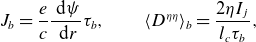 \begin{align} J_b=\frac {e}{c}\frac {\textrm { d} \psi }{\textrm { d} r}\tau _b, \qquad \langle D^{\eta \eta }\rangle _b=\frac {2 \eta I_j}{l_c \tau _{b}}, \end{align}
with $I_j$
defined in the first (2.26), and bounce time
$I_j$
defined in the first (2.26), and bounce time $\tau _b$
together with bounce-averaged radial drift velocity
$\tau _b$
together with bounce-averaged radial drift velocity $\langle v_g^r\rangle _b$
are given by (3.56) with the omission of class index
$\langle v_g^r\rangle _b$
are given by (3.56) with the omission of class index $k$
.
$k$
.
It should be noted that, due to the use of field aligned (Clebsch-like) spatial variables, both, $\langle v_g^r\rangle _b$
and
$\langle v_g^r\rangle _b$
and $\langle v_g^{\vartheta _0}\rangle _b$
can be evaluated here along the field lines (see (Shaing Reference Shaing2015; Calvo et al. Reference Calvo, Parra, Velasco and Alonso2017; d’Herbemont et al. Reference d’Herbemont, Parra, Calvo and Velasco2022)). On the contrary, for the non-aligned variables (periodic flux coordinates) tangential components of the bounce-averaged drift should be evaluated over the real bounce orbit with finite Larmor radius, which is in contrast to
$\langle v_g^{\vartheta _0}\rangle _b$
can be evaluated here along the field lines (see (Shaing Reference Shaing2015; Calvo et al. Reference Calvo, Parra, Velasco and Alonso2017; d’Herbemont et al. Reference d’Herbemont, Parra, Calvo and Velasco2022)). On the contrary, for the non-aligned variables (periodic flux coordinates) tangential components of the bounce-averaged drift should be evaluated over the real bounce orbit with finite Larmor radius, which is in contrast to $\langle v_g^r\rangle _b$
where this results only in a
$\langle v_g^r\rangle _b$
where this results only in a $\rho _L$
correction to (3.56). Such an evaluation is required to retain in the resulting precession frequency the effect of magnetic shear which is of the order one if
$\rho _L$
correction to (3.56). Such an evaluation is required to retain in the resulting precession frequency the effect of magnetic shear which is of the order one if $\Omega _E \lesssim \Omega _B$
(see (Shaing Reference Shaing2015; Albert et al. Reference Albert, Heyn, Kapper, Kasilov, Kernbichler and Martitsch2016; Martitsch et al. Reference Martitsch2016)). A way equivalent to bounce averaging velocity components is to use equation (3.48) of Morozov & Solov’ev (Reference Morozov and Solov’ev1966) resulting in
$\Omega _E \lesssim \Omega _B$
(see (Shaing Reference Shaing2015; Albert et al. Reference Albert, Heyn, Kapper, Kasilov, Kernbichler and Martitsch2016; Martitsch et al. Reference Martitsch2016)). A way equivalent to bounce averaging velocity components is to use equation (3.48) of Morozov & Solov’ev (Reference Morozov and Solov’ev1966) resulting in $\langle v_g^r\rangle _b = J_b^{-1}\partial J_\parallel /\partial \vartheta _0$
and
$\langle v_g^r\rangle _b = J_b^{-1}\partial J_\parallel /\partial \vartheta _0$
and $\langle v_g^{\vartheta _0}\rangle _b = - J_b^{-1}\partial J_\parallel /\partial r$
, where
$\langle v_g^{\vartheta _0}\rangle _b = - J_b^{-1}\partial J_\parallel /\partial r$
, where $J_\parallel = m\oint \textrm {d} l\, v_\parallel$
is the parallel adiabatic invariant computed along the field line, which makes the Liouville theorem
$J_\parallel = m\oint \textrm {d} l\, v_\parallel$
is the parallel adiabatic invariant computed along the field line, which makes the Liouville theorem $\partial (J_b \langle v_g^r\rangle _b)/\partial r + \partial (J_b \langle v_g^{\vartheta _0}\rangle _b)/\partial \vartheta _0 = 0$
obvious.
$\partial (J_b \langle v_g^r\rangle _b)/\partial r + \partial (J_b \langle v_g^{\vartheta _0}\rangle _b)/\partial \vartheta _0 = 0$
obvious.
Equation (5.1) means that off-set effect is generally non-local, i.e. radial transport due to entrapping of passing particles at some given surface is produced in some radial range $\delta r_c$
(radial correlation length) which in the
$\delta r_c$
(radial correlation length) which in the $1/\nu$
regime is of the order
$1/\nu$
regime is of the order $\delta r_c \sim \tau _d \langle v_g^r\rangle _b$
, where
$\delta r_c \sim \tau _d \langle v_g^r\rangle _b$
, where $\tau _d \sim \varepsilon _M/\nu$
is the de-trapping time, and, at lower collisionalities, where
$\tau _d \sim \varepsilon _M/\nu$
is the de-trapping time, and, at lower collisionalities, where $\langle v_g^{\vartheta _0}\rangle _b \gt 1/\tau _d$
and mild electric fields,
$\langle v_g^{\vartheta _0}\rangle _b \gt 1/\tau _d$
and mild electric fields, $\Omega _E \leqslant \Omega _B$
, is of the size of radial deviation of precessing trapped orbit which does not scale with Larmor radius and is fully determined by the magnetic field geometry. Thus, local ansatz (2.1) has a limited validity in the latter case where transport coefficients and bootstrap current need a non-local treatment, e.g. by Monte Carlo methods (Sasinowski & Boozer Reference Sasinowski and Boozer1995; Satake, Kanno & Sugama Reference Satake, Kanno and Sugama2008) (an exception is weakly perturbed tokamak equilibria where a quasi-local ansatz (Martitsch et al. Reference Martitsch2016) can be used retaining the boundary layer effects). Of course,
$\Omega _E \leqslant \Omega _B$
, is of the size of radial deviation of precessing trapped orbit which does not scale with Larmor radius and is fully determined by the magnetic field geometry. Thus, local ansatz (2.1) has a limited validity in the latter case where transport coefficients and bootstrap current need a non-local treatment, e.g. by Monte Carlo methods (Sasinowski & Boozer Reference Sasinowski and Boozer1995; Satake, Kanno & Sugama Reference Satake, Kanno and Sugama2008) (an exception is weakly perturbed tokamak equilibria where a quasi-local ansatz (Martitsch et al. Reference Martitsch2016) can be used retaining the boundary layer effects). Of course, $\delta r_c$
must be small compared with the plasma radius for the magnetic fields intended for the reactor, however, it is not necessarily small compared with the radial variation scale of the off-set which is quite sensitive to small modulations of the field and
$\delta r_c$
must be small compared with the plasma radius for the magnetic fields intended for the reactor, however, it is not necessarily small compared with the radial variation scale of the off-set which is quite sensitive to small modulations of the field and $\iota$
changes. One consequence of this non-locality is discussed in more details in § 6.
$\iota$
changes. One consequence of this non-locality is discussed in more details in § 6.
Equation (5.1) should be solved as is if the off-set is produced in the wide poloidal range containing the trapped–passing boundary layer, which is the case of almost aligned maxima discussed in §§ 3.3, 3.5 and 4.3. However, in a more typical case with a distinct global maximum (or two global maxima, which are also possible in stellarator symmetry), the width of the off-set region $\delta \vartheta$
is small (this is a typical width of a single strap in figures 21–24). Therefore, convective term with
$\delta \vartheta$
is small (this is a typical width of a single strap in figures 21–24). Therefore, convective term with $\langle v_g^{\vartheta _0}\rangle _b$
dominates over
$\langle v_g^{\vartheta _0}\rangle _b$
dominates over $\langle v_g^r\rangle _b$
which, therefore, can be ignored in (5.1) together with the dependence on
$\langle v_g^r\rangle _b$
which, therefore, can be ignored in (5.1) together with the dependence on $\vartheta _0$
of
$\vartheta _0$
of $\langle v_g^{\vartheta _0}\rangle _b \equiv \Omega ^\vartheta$
,
$\langle v_g^{\vartheta _0}\rangle _b \equiv \Omega ^\vartheta$
, $J_b$
and
$J_b$
and $D^{J_\perp J_\perp }$
, which should be taken at the global maximum point
$D^{J_\perp J_\perp }$
, which should be taken at the global maximum point $\vartheta _0=\vartheta _{\textrm{max}}$
, thus reducing (5.1) to
$\vartheta _0=\vartheta _{\textrm{max}}$
, thus reducing (5.1) to
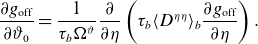 \begin{align} \frac {\partial g_{\text{off}}}{\partial \vartheta _0} = \frac {1}{\tau _b \Omega ^\vartheta } \frac {\partial }{\partial \eta }\left (\tau _b \langle D^{\eta \eta }\rangle _b \frac {\partial g_{\text{off}}}{\partial \eta }\right ). \end{align}
This can be done because $g_{\text{off}}$
is localized in
$g_{\text{off}}$
is localized in $\vartheta _0$
due to essentially trivial boundary conditions over
$\vartheta _0$
due to essentially trivial boundary conditions over $\eta$
at
$\eta$
at $|\vartheta _0-\vartheta _{\textrm{max}}| \gg \delta \vartheta$
. Therefore, solution to (5.3) in the infinite domain
$|\vartheta _0-\vartheta _{\textrm{max}}| \gg \delta \vartheta$
. Therefore, solution to (5.3) in the infinite domain $-\infty \lt \vartheta _0\lt \infty$
is sufficient to generalize the results of
$-\infty \lt \vartheta _0\lt \infty$
is sufficient to generalize the results of $g_{\text{off}}$
computations in the
$g_{\text{off}}$
computations in the $1/\nu$
regime for the case of finite precession frequencies (finite radial electric fields).
$1/\nu$
regime for the case of finite precession frequencies (finite radial electric fields).
For further estimates, we assume a fast precession case, $\Omega ^\vartheta \tau _d \gg \delta \vartheta$
(with
$\Omega ^\vartheta \tau _d \gg \delta \vartheta$
(with $\Omega ^\vartheta \tau _b \ll \delta \vartheta$
staying fulfilled, which is possible at low collisionalities where
$\Omega ^\vartheta \tau _b \ll \delta \vartheta$
staying fulfilled, which is possible at low collisionalities where $\tau _b \ll \tau _d$
), which would be the condition of the
$\tau _b \ll \tau _d$
), which would be the condition of the $\sqrt {\nu }$
transport regime (Galeev & Sagdeev Reference Galeev and Sagdeev1979) in case
$\sqrt {\nu }$
transport regime (Galeev & Sagdeev Reference Galeev and Sagdeev1979) in case $\delta \vartheta \sim 1$
but is established here for smaller precession frequencies due to
$\delta \vartheta \sim 1$
but is established here for smaller precession frequencies due to $\delta \vartheta \ll 1$
. In this case, solution is localized in
$\delta \vartheta \ll 1$
. In this case, solution is localized in $\eta$
near the matching boundary
$\eta$
near the matching boundary $\eta _m$
, and we can ignore class transitions which occur in the well trapped particle domain and also set
$\eta _m$
, and we can ignore class transitions which occur in the well trapped particle domain and also set $\eta =\eta _m$
in all the coefficients. Introducing the dimensionless variables as follows:
$\eta =\eta _m$
in all the coefficients. Introducing the dimensionless variables as follows:
 \begin{align} y=\frac {\vartheta -\vartheta _{\textrm{max}}}{\delta \vartheta } \textrm { sign}(\Omega ^\vartheta ), \qquad x = \left (\frac {|\Omega ^\vartheta |}{\delta \vartheta \langle D^{\eta \eta }\rangle _b}\right )^{1/2}(\eta -\eta _m), \end{align}
equation (5.3) is reduced to
 \begin{align} \frac {\partial g_{\text{off}}}{\partial y}=\frac {\partial ^2 g_{\text{off}}}{\partial x^2}, \end{align}
where $0 \lt x \lt \infty$
,
$0 \lt x \lt \infty$
, $-\infty \lt y \lt \infty$
, and the boundary conditions are
$-\infty \lt y \lt \infty$
, and the boundary conditions are $g_{\text{off}}(0,y)=g_{\text{off}}^{1/\nu }(\vartheta _{\textrm{max}} + y\,\delta \vartheta \,\textrm { sign}(\Omega ^\vartheta ),\eta _m)$
and
$g_{\text{off}}(0,y)=g_{\text{off}}^{1/\nu }(\vartheta _{\textrm{max}} + y\,\delta \vartheta \,\textrm { sign}(\Omega ^\vartheta ),\eta _m)$
and $g_{\text{off}}(x,-\infty )=0$
, so that solution is localized in the range
$g_{\text{off}}(x,-\infty )=0$
, so that solution is localized in the range $|y|\lesssim 1$
. Since the solution is also localized in the range
$|y|\lesssim 1$
. Since the solution is also localized in the range $x \lesssim 1$
, the second of (5.4) results in the localization range
$x \lesssim 1$
, the second of (5.4) results in the localization range $\eta -\eta _m \lt \delta _E \Delta \eta _{tr}$
, where
$\eta -\eta _m \lt \delta _E \Delta \eta _{tr}$
, where $\Delta \eta _{tr} \sim \varepsilon _t^{1/2} \eta _b$
is the width of trapped particle domain and
$\Delta \eta _{tr} \sim \varepsilon _t^{1/2} \eta _b$
is the width of trapped particle domain and $\delta _E \ll 1$
is the attenuation factor due to the precession (we assume here
$\delta _E \ll 1$
is the attenuation factor due to the precession (we assume here $\varepsilon _M \sim \varepsilon _t$
for simplicity). This reduction of the
$\varepsilon _M \sim \varepsilon _t$
for simplicity). This reduction of the $\eta$
integration range of
$\eta$
integration range of $g_{\text{off}} s_{(1)}$
effectively contributing to the Ware-pinch coefficient (2.11) respectively reduces its value by
$g_{\text{off}} s_{(1)}$
effectively contributing to the Ware-pinch coefficient (2.11) respectively reduces its value by $\delta _E$
as compared with the
$\delta _E$
as compared with the $1/\nu$
regime. Explicitly, this factor is
$1/\nu$
regime. Explicitly, this factor is
 \begin{align} \delta _E \sim \left (\frac {v\delta \vartheta }{l_c|\Omega ^\vartheta |}\right )^{1/2} \sim \left (\frac {v \nu _\ast }{N R|\Omega ^\vartheta |}\right )^{1/2}, \end{align}
where $N \sim 1/\delta \vartheta$
is the number of toroidal turns within a given off-set pattern. The overall trend of the Ware-pinch off-set with the reduction of
$N \sim 1/\delta \vartheta$
is the number of toroidal turns within a given off-set pattern. The overall trend of the Ware-pinch off-set with the reduction of $\nu _\ast$
is obtained with the account of switching off-set patterns and thus increasing
$\nu _\ast$
is obtained with the account of switching off-set patterns and thus increasing $N$
in (5.6) according to the first (4.6). Thus, the normalized maximum off-set (4.12) is reduced from its value in
$N$
in (5.6) according to the first (4.6). Thus, the normalized maximum off-set (4.12) is reduced from its value in $1/\nu$
regime to
$1/\nu$
regime to
 \begin{align} \frac {\lambda _{\text{off}}^{\textrm{max}}}{\lambda _{bB}^{\text{tok}}}\sim \iota \delta _E \sim \iota \varepsilon _t^{-3/20} \nu _\ast ^{3/5} \left (\frac {v}{R|\Omega ^\vartheta |}\right )^{1/2}, \end{align}
i.e. $\lambda _{bB}$
converges with decreasing collisionality to the Shaing–Callen limit. It should be noted that bootstrap resonances should still be removed from the asymptotic
$\lambda _{bB}$
converges with decreasing collisionality to the Shaing–Callen limit. It should be noted that bootstrap resonances should still be removed from the asymptotic $\lambda _{bB}$
for the same reason as discussed in § 4.4. In this case, in addition to pitch-angle scattering limiting the effective orbit length contributing to the resonance in the power low spectral decay region, also the precession de-correlates the resonant particles, effectively removing them from that region.
$\lambda _{bB}$
for the same reason as discussed in § 4.4. In this case, in addition to pitch-angle scattering limiting the effective orbit length contributing to the resonance in the power low spectral decay region, also the precession de-correlates the resonant particles, effectively removing them from that region.
In case of nearly aligned maxima, poloidal width of the off-set region in (5.6) is not small anymore, $\delta \vartheta \sim 1$
or, equivalently,
$\delta \vartheta \sim 1$
or, equivalently, $N\sim 1$
. Thus, using the
$N\sim 1$
. Thus, using the $1/\nu$
regime estimate (4.22) we obtain the scaling for normalized off-set due to violation of ripple equivalence as
$1/\nu$
regime estimate (4.22) we obtain the scaling for normalized off-set due to violation of ripple equivalence as
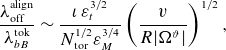 \begin{align} \frac {\lambda _{\text{off}}^{\text{align}}}{\lambda _{bB}^{\text{tok}}}\sim \frac {\iota \; \varepsilon _t^{3/2}}{N_{\text{tor}}^{1/2}\varepsilon _M^{3/4}} \left (\frac {v}{R|\Omega ^\vartheta |}\right )^{1/2}, \end{align}
which means that the off-set does not vanish but saturates with reducing collisionality at a rather high level due to the ratio of bounce frequency to the precession frequency in the last factor.
To verify the off-set attenuation model in case of a single off-set pattern with fixed $N$
in (5.6), we apply this model to DKES results in figure 4 of Helander et al. (Reference Helander, Geiger and Maassberg2011) where the dominant pattern appears to be unchanged in the whole range of
$N$
in (5.6), we apply this model to DKES results in figure 4 of Helander et al. (Reference Helander, Geiger and Maassberg2011) where the dominant pattern appears to be unchanged in the whole range of $\nu _\ast$
. The normalized bootstrap coefficient
$\nu _\ast$
. The normalized bootstrap coefficient $D_{31}^\ast \equiv \lambda _{bB}/\lambda _{bB}^{\text{tok}}$
in this figure, where the precession is purely due to the
$D_{31}^\ast \equiv \lambda _{bB}/\lambda _{bB}^{\text{tok}}$
in this figure, where the precession is purely due to the ${\textbf {E}}\times {\textbf {B}}$
drift,
${\textbf {E}}\times {\textbf {B}}$
drift, $\Omega ^\vartheta = \Omega _E \propto E_r$
, is represented using the scaling of attenuation factor (5.6) with collisionality and radial electric field
$\Omega ^\vartheta = \Omega _E \propto E_r$
, is represented using the scaling of attenuation factor (5.6) with collisionality and radial electric field $\delta _E \propto (\nu _\ast /E_r)^{1/2}$
as follows:
$\delta _E \propto (\nu _\ast /E_r)^{1/2}$
as follows:
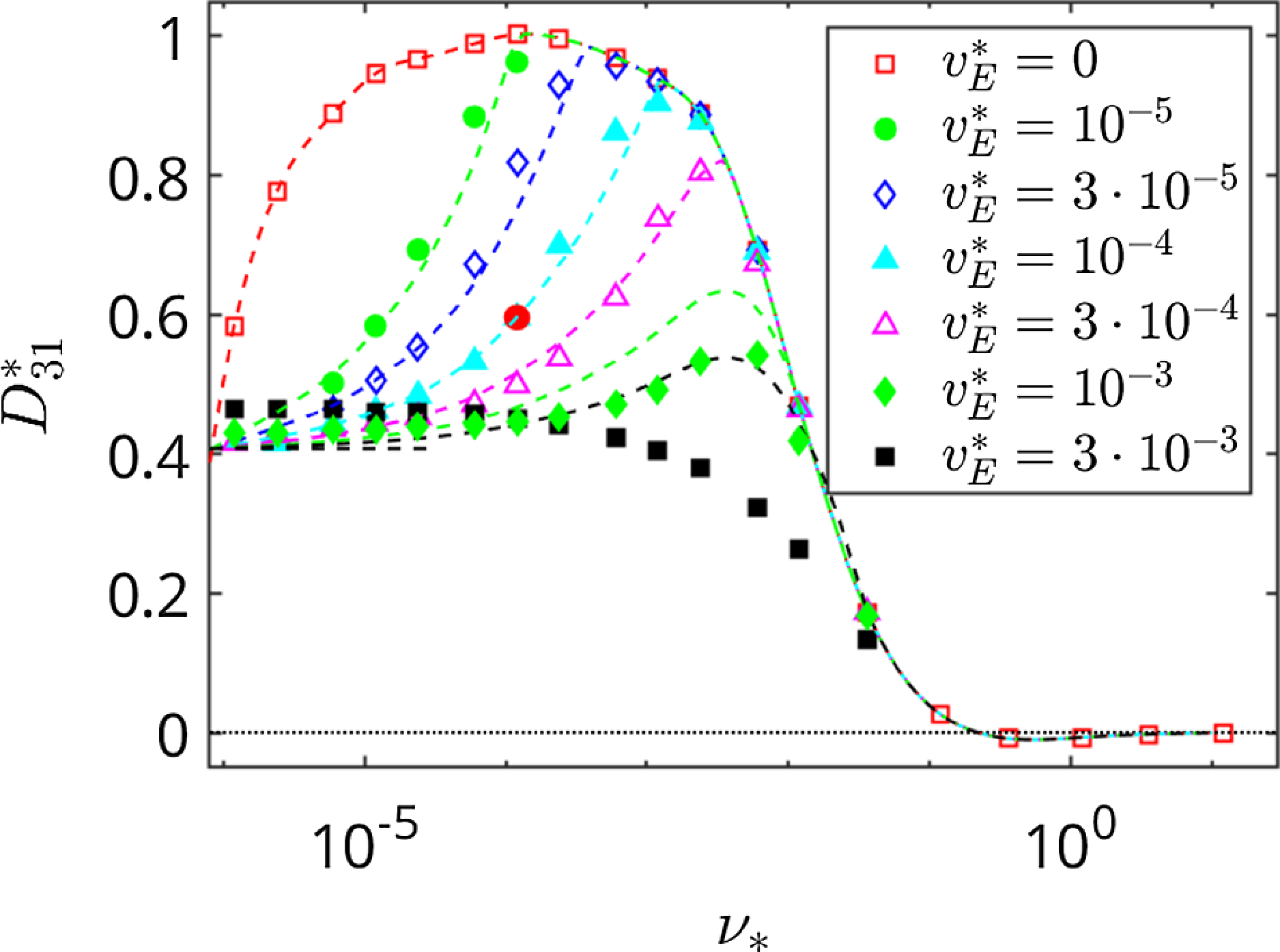
Figure 31. Attenuation test for the case in figure 4 of Helander et al. (Reference Helander, Geiger and Maassberg2011). Normalized electric field values (Mach numbers $v_E^\ast =cE_r/(vB)$
) are defined in the legend. Dashed lines show the result of scaling in (5.9) with the reference point shown by a red circle.
$v_E^\ast =cE_r/(vB)$
) are defined in the legend. Dashed lines show the result of scaling in (5.9) with the reference point shown by a red circle.
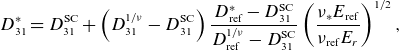 \begin{align} D^\ast _{31} = D_{31}^{\text{SC}}+\left (D_{31}^{1/\nu }- D_{\textrm {31}}^{\text{SC}}\right ) \frac {D^\ast _{\text{ref}}-D_{\textrm {31}}^{\text{SC}}}{D_{\text{ref}}^{1/\nu }-D_{\textrm{31}}^{\text{SC}}} \left (\frac {\nu _\ast E_{\text{ref}}}{\nu _{\text{ref}} E_r}\right )^{1/2}, \end{align}
where $D_{31}^{\text{SC}}$
is the Shaing–Callen asymptotic value of
$D_{31}^{\text{SC}}$
is the Shaing–Callen asymptotic value of $D^\ast _{31}$
,
$D^\ast _{31}$
, $D_{31}^{1/\nu }$
is the actual value in the
$D_{31}^{1/\nu }$
is the actual value in the $1/\nu$
regime,
$1/\nu$
regime, $\nu _{\text{ref}}$
and
$\nu _{\text{ref}}$
and $E_{\text{ref}}$
are the values of
$E_{\text{ref}}$
are the values of $\nu _\ast$
and
$\nu _\ast$
and $E_r$
for a single reference point in the plot and
$E_r$
for a single reference point in the plot and $D_{\text{ref}}^\ast$
and
$D_{\text{ref}}^\ast$
and $D_{\text{ref}}^{1/\nu }$
are the values of
$D_{\text{ref}}^{1/\nu }$
are the values of $D^\ast _{31}$
for
$D^\ast _{31}$
for $(\nu _\ast, E_r)=(\nu _{\text{ref}},E_{\text{ref}})$
and
$(\nu _\ast, E_r)=(\nu _{\text{ref}},E_{\text{ref}})$
and $(\nu _\ast, E_r)=(\nu _{\text{ref}},0)$
, respectively. As one can see in figure 31, scaling (5.9) well represents the results with mild electric field but fails for two largest values of
$(\nu _\ast, E_r)=(\nu _{\text{ref}},0)$
, respectively. As one can see in figure 31, scaling (5.9) well represents the results with mild electric field but fails for two largest values of $v_E^\ast$
where the (tokamak like) boundary layer off-set (Helander et al. Reference Helander, Geiger and Maassberg2011) becomes important (see also figure 19) and where the condition
$v_E^\ast$
where the (tokamak like) boundary layer off-set (Helander et al. Reference Helander, Geiger and Maassberg2011) becomes important (see also figure 19) and where the condition $\Omega _E \tau _b /\delta \vartheta \ll 1$
becomes violated.
$\Omega _E \tau _b /\delta \vartheta \ll 1$
becomes violated.
6. Off-set in the direct problem, bootstrap effect at the magnetic axis
We discuss now the off-set in the direct (bootstrap) problem qualitatively. Since the off-set in the Ware-pinch problem is driven by the asymmetry of the entrapping of passing particles, off-set in the bootstrap problem is driven by the asymmetry in the inverse process of trapped particle detrapping. Similarly, there are two (same) reasons for this asymmetry. First is the asymmetry of local maxima limiting ripple domains which leads to the detrapping in the direction of the lower maximum. The second one is connected with the violation of ripple equivalence, $A_j = 1$
, and, consequently, to the asymmetry of entrapping and further detrapping in the neighboring ripples. We estimate now only the first, simpler effect.
$A_j = 1$
, and, consequently, to the asymmetry of entrapping and further detrapping in the neighboring ripples. We estimate now only the first, simpler effect.
For the equilibrium (Maxwellian) particle distribution which is constant on the flux surface, the detrapping process is balanced by entrapping of passing particles leading to zero phase space fluxes (detailed equilibrium) and, respectively, to zero parallel current. In the presence of radial gradient, the distribution function of trapped particles is not constant on the flux surface anymore. It is larger in the region with positive bounce-averaged radial drift, and smaller where it is negative. In stellarator symmetry, it is obvious that particles are detrapped in those regions in opposite directions, thus leading to the overall shift of passing particle distribution and, respectively, to the parallel current. Destroyed symmetry of the ripple wells is described by the source term $s_{(1)}$
, (2.4), which generates ‘anti-particles’ in the wells with
$s_{(1)}$
, (2.4), which generates ‘anti-particles’ in the wells with $\langle v_g^r\rangle _b \gt 0$
and ‘particles’ where
$\langle v_g^r\rangle _b \gt 0$
and ‘particles’ where $\langle v_g^r\rangle _b \lt 0$
. In the asymptotic
$\langle v_g^r\rangle _b \lt 0$
. In the asymptotic $1/\nu$
regime, these particles and anti-particles produced by the source term
$1/\nu$
regime, these particles and anti-particles produced by the source term $s_{(1)}$
within ripple wells can leave these wells only through boundary layers between classes, where they are re-distributed and annihilated. As we saw in §§ 2.2.1 and 2.3.1, parallel flows within these boundary layers make a contribution of the order one to the equilibrium Pfirsch–Schlüter current. This changes at finite collisionality where ‘relevant ripples’ appear with both limiting local maxima entering the trapped–passing boundary layer. Re-distribution of particles and anti-particles between ‘relevant’ ripples occurs then through the trapped–passing boundary layer (this layer is empty in the asymptotic
$s_{(1)}$
within ripple wells can leave these wells only through boundary layers between classes, where they are re-distributed and annihilated. As we saw in §§ 2.2.1 and 2.3.1, parallel flows within these boundary layers make a contribution of the order one to the equilibrium Pfirsch–Schlüter current. This changes at finite collisionality where ‘relevant ripples’ appear with both limiting local maxima entering the trapped–passing boundary layer. Re-distribution of particles and anti-particles between ‘relevant’ ripples occurs then through the trapped–passing boundary layer (this layer is empty in the asymptotic $1/\nu$
regime) causing the parallel flow there and respective asymmetry of the distribution function over the pitch parameter
$1/\nu$
regime) causing the parallel flow there and respective asymmetry of the distribution function over the pitch parameter $\lambda$
. Such an odd distribution in the boundary layer,
$\lambda$
. Such an odd distribution in the boundary layer, $g^{\text{odd}}$
, serves as a boundary condition which shifts from zero the odd part of the distribution function in the whole passing particle domain thus generating a bootstrap current.
$g^{\text{odd}}$
, serves as a boundary condition which shifts from zero the odd part of the distribution function in the whole passing particle domain thus generating a bootstrap current.
We can estimate $g^{\text{odd}}$
in the boundary layer using the argument at the end of § 2.2.1 as
$g^{\text{odd}}$
in the boundary layer using the argument at the end of § 2.2.1 as $g^{\text{odd}} \sim H_j(\eta _{\textrm{loc}})/\delta \eta _{\text{ref}}$
, where
$g^{\text{odd}} \sim H_j(\eta _{\textrm{loc}})/\delta \eta _{\text{ref}}$
, where $H_j(\eta _{\textrm{loc}})$
is the collisional flux through class boundary
$H_j(\eta _{\textrm{loc}})$
is the collisional flux through class boundary $\eta =\eta _{\textrm{loc}}\equiv \max (\eta _j,\eta _{j+1})$
of the relevant ripple (which corresponds to the off-set domain in the adjoint problem) with
$\eta =\eta _{\textrm{loc}}\equiv \max (\eta _j,\eta _{j+1})$
of the relevant ripple (which corresponds to the off-set domain in the adjoint problem) with
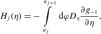 \begin{align} H_j(\eta )=-\int \limits _{\varphi _j}^{\varphi _{j+1}}\textrm { d}\varphi D_\eta \frac {\partial g_{-1}}{\partial \eta }, \end{align}
and $g_{-1}$
being the leading-order solution of direct problem (2.27), and where
$g_{-1}$
being the leading-order solution of direct problem (2.27), and where $\delta \eta _{\text{ref}}$
is the width of the trapped–passing boundary layer in the “main region”. Since the odd part of passing particle distribution driven by
$\delta \eta _{\text{ref}}$
is the width of the trapped–passing boundary layer in the “main region”. Since the odd part of passing particle distribution driven by $g^{\text{odd}}$
at the trapped–passing boundary is independent of
$g^{\text{odd}}$
at the trapped–passing boundary is independent of $\eta$
and is, therefore, equal to
$\eta$
and is, therefore, equal to $g^{\text{odd}}$
, we can estimate the parallel current density off-set using (2.38) as
$g^{\text{odd}}$
, we can estimate the parallel current density off-set using (2.38) as $j_\parallel ^{\text{off}} \approx C_\parallel g^{\text{odd}}$
, and the respective off-set of the normalized bootstrap coefficient in (2.42) as
$j_\parallel ^{\text{off}} \approx C_\parallel g^{\text{odd}}$
, and the respective off-set of the normalized bootstrap coefficient in (2.42) as $\lambda _{\text{off}} \sim g^{\text{odd}}/\rho _L \sim H_j(\eta _{\textrm{loc}})/(\rho _L \delta \eta _{\text{ref}})$
. Naturally, the same result is obtained for the off-set (3.54) in the adjoint problem using for
$\lambda _{\text{off}} \sim g^{\text{odd}}/\rho _L \sim H_j(\eta _{\textrm{loc}})/(\rho _L \delta \eta _{\text{ref}})$
. Naturally, the same result is obtained for the off-set (3.54) in the adjoint problem using for $w^{(j)}_{\text{off}}$
the second equality (3.55) and for
$w^{(j)}_{\text{off}}$
the second equality (3.55) and for $g_{\text{off}}^{(j)}$
(3.28) where
$g_{\text{off}}^{(j)}$
(3.28) where $\alpha _j^\pm \sim 1$
in case of the maximum off-set, and constant (3.18) is
$\alpha _j^\pm \sim 1$
in case of the maximum off-set, and constant (3.18) is
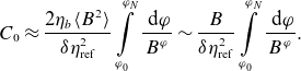 \begin{align} C_0 \approx \frac {2\eta _b \langle B^2\rangle }{\delta \eta _{\text{ref}}^2}\int \limits _{\varphi _0}^{\varphi _N}\frac {\textrm { d}\varphi }{B^\varphi } \sim \frac {B}{\delta \eta _{\text{ref}}^2}\int \limits _{\varphi _0}^{\varphi _N}\frac {\textrm { d}\varphi }{B^\varphi }. \end{align}
Note that effect of particle precession reducing the off-set in the adjoint problem is also the same in the direct problem where it causes re-distribution of trapped “particles” and “anti-particles” between trapping domains via the rotation within the flux surface thus reducing the collisional fluxes into class boundaries as compared with their maximum $1/\nu$
values
$1/\nu$
values $H_j(\eta _{\textrm{loc}})$
.
$H_j(\eta _{\textrm{loc}})$
.
Recalling now definitions (2.26) and (2.4) of the normalized collisional velocity space flux $H_j$
(see also (3.55) and (3.57)) we can approximately relate
$H_j$
(see also (3.55) and (3.57)) we can approximately relate $H_j$
to the radial correlation length in the off-set well
$H_j$
to the radial correlation length in the off-set well $\delta r_{cj} \sim \tau _{dj} \langle v_g^r\rangle _{bj}$
as follows,
$\delta r_{cj} \sim \tau _{dj} \langle v_g^r\rangle _{bj}$
as follows, $H_j \sim \tau _{bj} \langle v_g^r\rangle _{bj} \Delta \eta _j \sim \delta r_{cj} \delta \eta _j^2/\Delta \eta _j$
where
$H_j \sim \tau _{bj} \langle v_g^r\rangle _{bj} \Delta \eta _j \sim \delta r_{cj} \delta \eta _j^2/\Delta \eta _j$
where $\tau _{bj}$
and
$\tau _{bj}$
and $\langle v_g^r\rangle _{bj}$
are bounce time and bounce-averaged velocity (3.56),
$\langle v_g^r\rangle _{bj}$
are bounce time and bounce-averaged velocity (3.56), $\tau _{dj} \sim \tau _{bj} (\Delta \eta _j/\delta \eta _j)^2$
is the detrapping time,
$\tau _{dj} \sim \tau _{bj} (\Delta \eta _j/\delta \eta _j)^2$
is the detrapping time, $\Delta \eta _j\sim \varepsilon _M\eta _b$
is the off-set well depth and
$\Delta \eta _j\sim \varepsilon _M\eta _b$
is the off-set well depth and $\delta \eta _j$
is boundary layer width in the off-set domain (see (3.26) and (3.20)). Thus,
$\delta \eta _j$
is boundary layer width in the off-set domain (see (3.26) and (3.20)). Thus, $g^{\text{odd}} \sim \delta r_{cj} \delta \eta _j/(A_j \Delta \eta _j)$
with the aspect ratio
$g^{\text{odd}} \sim \delta r_{cj} \delta \eta _j/(A_j \Delta \eta _j)$
with the aspect ratio $A_j=\delta \eta _{\text{ref}}/\delta \eta _j$
, and we can estimate current density as follows:
$A_j=\delta \eta _{\text{ref}}/\delta \eta _j$
, and we can estimate current density as follows:
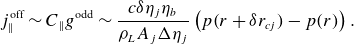 \begin{align} j_\parallel ^{\text{off}} \sim C_\parallel g^{\text{odd}} \sim \frac {c \delta \eta _j\eta _b}{\rho _L A_j \Delta \eta _j}\left (p(r+\delta r_{cj})-p(r)\right ). \end{align}
This formula actually reverses local transport ansatz (2.1) which assumes infinitesimal correlation length, and manifests the fact that variation of the distribution function on a given flux surface (along the field line) from its equilibrium value is because its value in the ripple wells is determined by the values of equilibrium distribution function at the neighboring flux surfaces displaced by the correlation length (strictly speaking, connection of parallel current density to the pressure gradient is non-local, $j_\parallel ^{\text{off}} = \int \textrm { d} r^\prime K(r,r^\prime ) p(r^\prime )$
, with the kernel
$j_\parallel ^{\text{off}} = \int \textrm { d} r^\prime K(r,r^\prime ) p(r^\prime )$
, with the kernel $K(r,r^\prime )$
localized within
$K(r,r^\prime )$
localized within $|r^\prime -r| \lesssim \delta r_{cj}$
). Thus, this variation and resulting parallel current need not disappear at the magnetic axis where
$|r^\prime -r| \lesssim \delta r_{cj}$
). Thus, this variation and resulting parallel current need not disappear at the magnetic axis where $\textrm { d} p/\textrm { d} r = 0$
. Expanding
$\textrm { d} p/\textrm { d} r = 0$
. Expanding $p(r+\delta r_{cj})$
to the next order, we obtain parallel current on axis as
$p(r+\delta r_{cj})$
to the next order, we obtain parallel current on axis as
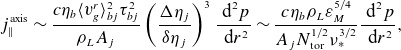 \begin{align} j_\parallel ^{\text{axis}} \sim \frac {c \eta _b \langle v_g^r\rangle _{bj}^2 \tau _{bj}^2}{\rho _L A_j} \left (\frac {\Delta \eta _j}{\delta \eta _j}\right )^{3}\frac {\textrm { d}^2 p}{\textrm { d} r^2} \sim \frac {c \eta _b \rho _L \varepsilon _M^{5/4}}{A_j N_{\text{tor}}^{1/2}\nu _\ast ^{3/2}} \frac {\textrm { d}^2 p}{\textrm { d} r^2}, \end{align}
where we estimated $\langle v_g^r\rangle _{bj} \sim v \rho _L/R$
,
$\langle v_g^r\rangle _{bj} \sim v \rho _L/R$
, $\tau _{bj} \sim R/(v N_{\text{tor}} \varepsilon _M^{1/2})$
,
$\tau _{bj} \sim R/(v N_{\text{tor}} \varepsilon _M^{1/2})$
, $\Delta \eta _j \sim \eta _b\varepsilon _M$
and
$\Delta \eta _j \sim \eta _b\varepsilon _M$
and $\delta \eta _j \sim \eta _b \left (\nu _\ast /N_{\text{tor}}\right )^{1/2}\varepsilon _M^{1/4}$
, with
$\delta \eta _j \sim \eta _b \left (\nu _\ast /N_{\text{tor}}\right )^{1/2}\varepsilon _M^{1/4}$
, with $N_{\textrm {tor}}$
being the number of ripples. Further denoting
$N_{\textrm {tor}}$
being the number of ripples. Further denoting $\textrm { d}^2 p / \textrm { d} r^2 = p / L^2_{pa}$
and normalizing (6.4) to a typical tokamak bootstrap current value
$\textrm { d}^2 p / \textrm { d} r^2 = p / L^2_{pa}$
and normalizing (6.4) to a typical tokamak bootstrap current value $j_b^{\text{tok}} \sim c \eta _b \iota ^{-1}\varepsilon _t^{-1/2}\textrm { d} p /\textrm { d} r = c \eta _b p /(\iota \varepsilon _t^{1/2} L_p)$
, we obtain
$j_b^{\text{tok}} \sim c \eta _b \iota ^{-1}\varepsilon _t^{-1/2}\textrm { d} p /\textrm { d} r = c \eta _b p /(\iota \varepsilon _t^{1/2} L_p)$
, we obtain
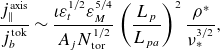 \begin{align} \frac {j_\parallel ^{\text{axis}}}{j_b^{\text{tok}}} \sim \frac {\iota \varepsilon _t^{1/2} \varepsilon _M^{5/4}}{A_j N_{\text{tor}}^{1/2}} \left (\frac {L_p}{L_{pa}}\right )^2 \frac {\rho ^\ast }{\nu _\ast ^{3/2}}, \end{align}
where $\rho ^\ast =\rho _L / L_p$
. Although this expression contains a small parameter
$\rho ^\ast =\rho _L / L_p$
. Although this expression contains a small parameter $\rho ^\ast$
in the numerator, it has another small parameter
$\rho ^\ast$
in the numerator, it has another small parameter $\nu _\ast ^{3/2}$
in the denominator so that current on axis is not vanishingly small. Estimating for parameters of the tokamak ASDEX Upgrade in the presence of the helical core with
$\nu _\ast ^{3/2}$
in the denominator so that current on axis is not vanishingly small. Estimating for parameters of the tokamak ASDEX Upgrade in the presence of the helical core with $\varepsilon _M \sim 0.01$
,
$\varepsilon _M \sim 0.01$
, $\iota \sim 0.5$
,
$\iota \sim 0.5$
, $\varepsilon _t \sim 0.25$
,
$\varepsilon _t \sim 0.25$
, $A_j = 1$
,
$A_j = 1$
, $N_{\textrm{tor}} = 2$
and central density
$N_{\textrm{tor}} = 2$
and central density $n_e = 3\cdot 10^{13}$
cm
$n_e = 3\cdot 10^{13}$
cm $^{-3}$
and temperature
$^{-3}$
and temperature $T_e = 5$
KeV resulting in
$T_e = 5$
KeV resulting in $\rho ^\ast =\rho _e^\ast \sim 2\cdot 10^{-4}$
and
$\rho ^\ast =\rho _e^\ast \sim 2\cdot 10^{-4}$
and $\nu _\ast \sim 3.5\cdot 10^{-3}$
, we get
$\nu _\ast \sim 3.5\cdot 10^{-3}$
, we get $\rho ^\ast \nu _\ast ^{-3/2} \approx 1$
so that
$\rho ^\ast \nu _\ast ^{-3/2} \approx 1$
so that $j_\parallel ^{\text{axis}}/j_b^{\text{tok}} \sim 5\cdot 10^{-4} (L_p/L_{pa})^2$
. Thus, for peaked
$j_\parallel ^{\text{axis}}/j_b^{\text{tok}} \sim 5\cdot 10^{-4} (L_p/L_{pa})^2$
. Thus, for peaked $T_e$
profiles (e.g. in the presence of central electron cyclotron heating) peaking factor
$T_e$
profiles (e.g. in the presence of central electron cyclotron heating) peaking factor $L_p/L_{pa} \sim 40$
is needed to make these currents comparable. Of course, in order to achieve
$L_p/L_{pa} \sim 40$
is needed to make these currents comparable. Of course, in order to achieve $j_\parallel ^{\text{axis}}$
, special conditions on the magnetic geometry are required in order to create, in particular, difference in correlation length
$j_\parallel ^{\text{axis}}$
, special conditions on the magnetic geometry are required in order to create, in particular, difference in correlation length $\delta r_j$
in different ripples.
$\delta r_j$
in different ripples.
Note that we have retained in the estimates (6.4) and (6.5) only the off-set effect but ignored the usual bootstrap mechanism where radial correlation length $\tau _{cj}$
corresponds to the banana width which is much smaller for electrons than
$\tau _{cj}$
corresponds to the banana width which is much smaller for electrons than $\tau _{cj}$
resulting from the
$\tau _{cj}$
resulting from the $1/\nu$
transport. However, this usual mechanism is not small for the ions whose radial orbit extent and, respectively, radial correlation length is much larger (with the orbits near the axis comprising a variety of classes even in an axisymmetric tokamak (Shaing, Ida & Sabbagh Reference Shaing, Ida and Sabbagh2015; Buchholz et al. Reference Buchholz, Kasilov, Kernbichler, Grabenwarter, Savchenko and Albert2022)), and, more importantly, who retain due to their high mass nearly all the momentum within the species during Coulomb collisions. For the axisymmetric devices, this mechanism generates the parallel ion flow (generally different from the
$1/\nu$
transport. However, this usual mechanism is not small for the ions whose radial orbit extent and, respectively, radial correlation length is much larger (with the orbits near the axis comprising a variety of classes even in an axisymmetric tokamak (Shaing, Ida & Sabbagh Reference Shaing, Ida and Sabbagh2015; Buchholz et al. Reference Buchholz, Kasilov, Kernbichler, Grabenwarter, Savchenko and Albert2022)), and, more importantly, who retain due to their high mass nearly all the momentum within the species during Coulomb collisions. For the axisymmetric devices, this mechanism generates the parallel ion flow (generally different from the $E\times B$
flow) but not the current since this flow is fully compensated by the electron flow driven by the collisional friction. However, if the toroidal ripple is present, it brakes the electrons leading to some steady current on axis if the ion flow is finite there. The latter is affected by ripple too via the neoclassical toroidal viscous torque (Shaing Reference Shaing2015; Albert et al. Reference Albert, Heyn, Kapper, Kasilov, Kernbichler and Martitsch2016; Martitsch et al. Reference Martitsch2016) which tends to bring the toroidal rotation velocity towards the (finite) intrinsic velocity driven by the ion temperature gradient. Due to the finite radial orbit width, finite gradients at surrounding flux surfaces result in finite ion rotation on axis which finally leads to a finite equilibrium current there. Generally, once the axial symmetry of the tokamak magnetic field is violated, there appear various mechanisms resulting in finite non-inductive toroidal current on axis which is necessary for the steady state tokamak operation, see, e.g. Weening & Boozer (Reference Weening and Boozer1992). At the same time, mechanisms discussed here are rather weak for that purpose which is better achieved with help of stellarator–tokamak hybrids (Ku & Boozer Reference Ku and Boozer2009; Henneberg & Plunk Reference Henneberg and Plunk2024; Liang et al. Reference Liang, Zhou, Dong, Zhu, Yu, Zhao and Dong2025).
$E\times B$
flow) but not the current since this flow is fully compensated by the electron flow driven by the collisional friction. However, if the toroidal ripple is present, it brakes the electrons leading to some steady current on axis if the ion flow is finite there. The latter is affected by ripple too via the neoclassical toroidal viscous torque (Shaing Reference Shaing2015; Albert et al. Reference Albert, Heyn, Kapper, Kasilov, Kernbichler and Martitsch2016; Martitsch et al. Reference Martitsch2016) which tends to bring the toroidal rotation velocity towards the (finite) intrinsic velocity driven by the ion temperature gradient. Due to the finite radial orbit width, finite gradients at surrounding flux surfaces result in finite ion rotation on axis which finally leads to a finite equilibrium current there. Generally, once the axial symmetry of the tokamak magnetic field is violated, there appear various mechanisms resulting in finite non-inductive toroidal current on axis which is necessary for the steady state tokamak operation, see, e.g. Weening & Boozer (Reference Weening and Boozer1992). At the same time, mechanisms discussed here are rather weak for that purpose which is better achieved with help of stellarator–tokamak hybrids (Ku & Boozer Reference Ku and Boozer2009; Henneberg & Plunk Reference Henneberg and Plunk2024; Liang et al. Reference Liang, Zhou, Dong, Zhu, Yu, Zhao and Dong2025).
7. Conclusion
To sum up, we can conclude that the bootstrap current in arbitrary three-dimensional toroidal fields does not converge to the asymptotic Shaing–Callen limit in the $1/\nu$
transport regime. The collisional current off-set being the difference between the actual bootstrap current and its collisionless asymptotic stays of the order of the bootstrap current in the equivalent tokamak and only oscillates aperiodically with changing
$1/\nu$
transport regime. The collisional current off-set being the difference between the actual bootstrap current and its collisionless asymptotic stays of the order of the bootstrap current in the equivalent tokamak and only oscillates aperiodically with changing $\log \nu _\ast$
. Moreover, for a set of configurations with aligned local magnetic field maxima (such that the global maximum is achieved at the flux surface on a line rather than at one or few points) the bootstrap current off-set diverges as
$\log \nu _\ast$
. Moreover, for a set of configurations with aligned local magnetic field maxima (such that the global maximum is achieved at the flux surface on a line rather than at one or few points) the bootstrap current off-set diverges as $\nu _\ast ^{-1/2}$
, as long as the condition of equivalent ripples (3.31) is not fulfilled (this condition is naturally fulfilled in axisymmetric and exactly quasi-symmetric fields). In turn, in the presence of orbit precession, in particular, due to a finite radial electric field, the off-set current converges to zero with reducing collisionality as
$\nu _\ast ^{-1/2}$
, as long as the condition of equivalent ripples (3.31) is not fulfilled (this condition is naturally fulfilled in axisymmetric and exactly quasi-symmetric fields). In turn, in the presence of orbit precession, in particular, due to a finite radial electric field, the off-set current converges to zero with reducing collisionality as $\nu _\ast ^{3/5} |\Omega ^\vartheta |^{-1/2}$
, which is in agreement with the results of numerical modeling by various codes (Beidler et al. Reference Beidler2011). Also, in the case of aligned maxima, the off-set does converge – not to zero but to a finite value which exceeds the equivalent tokamak current by a large factor
$\nu _\ast ^{3/5} |\Omega ^\vartheta |^{-1/2}$
, which is in agreement with the results of numerical modeling by various codes (Beidler et al. Reference Beidler2011). Also, in the case of aligned maxima, the off-set does converge – not to zero but to a finite value which exceeds the equivalent tokamak current by a large factor $\sim (v/R\Omega ^\vartheta )^{1/2} \sim \left (v_E^\ast \right )^{-1/2}$
, where
$\sim (v/R\Omega ^\vartheta )^{1/2} \sim \left (v_E^\ast \right )^{-1/2}$
, where $v_E^\ast = c E/(v B) \ll 1$
is the perpendicular Mach number.
$v_E^\ast = c E/(v B) \ll 1$
is the perpendicular Mach number.
The missing convergence of bootstrap current in the $1/\nu$
regime to the analytical collisionless asymptotic value is the consequence of two competing limits present in the problem. Namely, analytical derivations assume explicitly or implicitly that the field line is closed after a finite number of toroidal turns so that the mean free path strongly exceeds the period of the field line closure. As a consequence, the trapped–passing boundary layer width in velocity space
$1/\nu$
regime to the analytical collisionless asymptotic value is the consequence of two competing limits present in the problem. Namely, analytical derivations assume explicitly or implicitly that the field line is closed after a finite number of toroidal turns so that the mean free path strongly exceeds the period of the field line closure. As a consequence, the trapped–passing boundary layer width in velocity space $\delta \eta _{\text{ref}}$
is assumed infinitesimal such that all class-transition boundary layers centered around
$\delta \eta _{\text{ref}}$
is assumed infinitesimal such that all class-transition boundary layers centered around $\eta =\eta _c=1/B_{\textrm{loc}}$
coming from local field maxima
$\eta =\eta _c=1/B_{\textrm{loc}}$
coming from local field maxima $B_{\textrm{loc}}$
which are below the global maximum
$B_{\textrm{loc}}$
which are below the global maximum $B_{\textrm{max}}$
are clearly separated from the trapped–passing boundary layer centered at
$B_{\textrm{max}}$
are clearly separated from the trapped–passing boundary layer centered at $\eta =\eta _b=1/B_{\textrm{max}}$
. Obviously, this assumption cannot be fulfilled at irrational surfaces where the field line closure period is indeed infinite but the mean free path length stays finite, and where class-transition boundary layers inevitably interact with the trapped–passing boundary layer, leading to the bootstrap current off-set. This contradiction between two limits is manifested in the fractal spatial structure of the collisionless solutions for the distribution function, which is the fractal within the irrational flux surface in the adjoint approach (Helander et al. Reference Helander, Geiger and Maassberg2011) and has a fractal dependence on radius (leading to bootstrap resonances) also in the direct approach (Shaing & Callen Reference Shaing and Callen1983; Boozer & Gardner Reference Boozer and Gardner1990).
$\eta =\eta _b=1/B_{\textrm{max}}$
. Obviously, this assumption cannot be fulfilled at irrational surfaces where the field line closure period is indeed infinite but the mean free path length stays finite, and where class-transition boundary layers inevitably interact with the trapped–passing boundary layer, leading to the bootstrap current off-set. This contradiction between two limits is manifested in the fractal spatial structure of the collisionless solutions for the distribution function, which is the fractal within the irrational flux surface in the adjoint approach (Helander et al. Reference Helander, Geiger and Maassberg2011) and has a fractal dependence on radius (leading to bootstrap resonances) also in the direct approach (Shaing & Callen Reference Shaing and Callen1983; Boozer & Gardner Reference Boozer and Gardner1990).
The off-set which appears at any collisionality at irrational surfaces (or, equivalently, long enough rational field lines) results from the collisional particle exchange between trapped and passing particle domains in the velocity space. This exchange occurs through the boundary layer which, in usual configurations with global magnetic field maximum achieved in one or few points, is localized at the flux surface in some vicinity (contact region or ‘hot spot’) around this maximum such that field line returns to this vicinity after $N \propto \nu _\ast ^{-1/5} \ll 1$
toroidal turns. The off-set of the distribution function formed between two return points is the largest from all configurations,
$N \propto \nu _\ast ^{-1/5} \ll 1$
toroidal turns. The off-set of the distribution function formed between two return points is the largest from all configurations, $g_{\text{off}} \propto \nu _\ast ^{-3/5}$
, but it does not lead to the divergence of bootstrap current because the normalized integral of bounce-averaged velocity over the long off-set domain,
$g_{\text{off}} \propto \nu _\ast ^{-3/5}$
, but it does not lead to the divergence of bootstrap current because the normalized integral of bounce-averaged velocity over the long off-set domain, $w_{\text{off}} \propto \nu _\ast ^{3/5} \ll 1$
is the smallest and balances the former in resulting bootstrap coefficient
$w_{\text{off}} \propto \nu _\ast ^{3/5} \ll 1$
is the smallest and balances the former in resulting bootstrap coefficient $\lambda _{\text{off}} \propto g_{\text{off}} w_{\text{off}}$
. This compensation disappears in case of nearly aligned maxima, where boundary layer contact regions turn into stripes with much larger area than ‘hot spot’ in the usual case. These contact regions cut the field lines into much shorter off-set domains with the length about a single toroidal period, such that
$\lambda _{\text{off}} \propto g_{\text{off}} w_{\text{off}}$
. This compensation disappears in case of nearly aligned maxima, where boundary layer contact regions turn into stripes with much larger area than ‘hot spot’ in the usual case. These contact regions cut the field lines into much shorter off-set domains with the length about a single toroidal period, such that $w_{\text{off}}$
does not scale with collisionality anymore, but the distribution function still does,
$w_{\text{off}}$
does not scale with collisionality anymore, but the distribution function still does, $g_{\text{off}} \propto \nu _\ast ^{-1/2}$
. Although this scaling is weaker than in the usual case, missing compensation leads to
$g_{\text{off}} \propto \nu _\ast ^{-1/2}$
. Although this scaling is weaker than in the usual case, missing compensation leads to $\nu _\ast ^{-1/2}$
divergence of the resulting bootstrap current. This diverging part is respectively reduced if bounce-averaged drift is minimized for trapped particles, which is naturally the case in quasi-symmetric configurations.
$\nu _\ast ^{-1/2}$
divergence of the resulting bootstrap current. This diverging part is respectively reduced if bounce-averaged drift is minimized for trapped particles, which is naturally the case in quasi-symmetric configurations.
For the analysis of boundary layer effects and resulting off-set of bootstrap current we have developed a simplified propagator method, and obtained with its help, besides the condition of equivalent ripples (3.31) formulated earlier in Helander et al. (Reference Helander, Geiger and Maassberg2011) as a property of ideal quasi-isodynamic stellarators leading there to a tokamak-like bootstrap effect, also the expression (3.53) for the off-set of the distribution function in the case of imperfectly aligned local maxima and a slightly violated ripple equivalence condition (3.53) together with the respective estimate (4.22) of the resulting off-set of bootstrap coefficient in the case of the devices with non-optimized bounce-averaged radial drift of trapped particles. Actually, the case of nearly aligned maxima is the most interesting from the point of view of good fusion alpha particle confinement. This is naturally the case in quasi-symmetric configurations and in quasi-isodynamic configurations with poloidally closed of contours of $B$
. As can be seen from condition (4.22), the way to avoid the off-set of bootstrap current in such configurations is to align the maxima accurately and to realize ripple equivalence condition (3.31). The latter condition is almost the same as the condition of being tied to the flux surface contours of the parallel adiabatic invariant
$B$
. As can be seen from condition (4.22), the way to avoid the off-set of bootstrap current in such configurations is to align the maxima accurately and to realize ripple equivalence condition (3.31). The latter condition is almost the same as the condition of being tied to the flux surface contours of the parallel adiabatic invariant $J_\parallel$
for barely passing particles which, once realized in the case of perfectly aligned maxima, would prevent collisionless trapped–passing particle transitions and resulting stochastic transport. The essential difference of the respective integral
$J_\parallel$
for barely passing particles which, once realized in the case of perfectly aligned maxima, would prevent collisionless trapped–passing particle transitions and resulting stochastic transport. The essential difference of the respective integral $I_j$
from
$I_j$
from $J_\parallel =m\oint \textrm {d} l\,v_\parallel$
is only in an extra
$J_\parallel =m\oint \textrm {d} l\,v_\parallel$
is only in an extra $1/B$
factor in the sub-integrand. Both conditions are naturally satisfied if quasi-symmetry conditions are realized exactly, which, however, cannot be achieved at all flux surfaces (Garren & Boozer Reference Garren and Boozer1991). More generally, these conditions are fulfilled simultaneously for perfectly omnigeneous fields (Cary & Shasharina Reference Cary and Shasharina1997; Helander & Nührenberg, Reference Helander and Nührenberg2009) being also an idealization (Cary & Shasharina Reference Cary and Shasharina1997).
$1/B$
factor in the sub-integrand. Both conditions are naturally satisfied if quasi-symmetry conditions are realized exactly, which, however, cannot be achieved at all flux surfaces (Garren & Boozer Reference Garren and Boozer1991). More generally, these conditions are fulfilled simultaneously for perfectly omnigeneous fields (Cary & Shasharina Reference Cary and Shasharina1997; Helander & Nührenberg, Reference Helander and Nührenberg2009) being also an idealization (Cary & Shasharina Reference Cary and Shasharina1997).
As a curious consequence of bootstrap off-set, we have shown in § 6 a possibility of a bootstrap effect at the magnetic axis due to a rather large radial correlation length of the orbits $\delta r_c$
at low plasma collisionalities where it scales in the
$\delta r_c$
at low plasma collisionalities where it scales in the $1/\nu$
regime as
$1/\nu$
regime as $\delta r_c \propto \rho _L / \nu _\ast$
and strongly exceeds the Larmor radius
$\delta r_c \propto \rho _L / \nu _\ast$
and strongly exceeds the Larmor radius $\rho _L$
. Thus, the bootstrap current on axis being vanishingly small in axisymmetric fields where, due to a vanishing gradient and
$\rho _L$
. Thus, the bootstrap current on axis being vanishingly small in axisymmetric fields where, due to a vanishing gradient and $\delta r_c \sim \rho _L$
, it scales as
$\delta r_c \sim \rho _L$
, it scales as $\rho _{Le}^2/L_p^2=(\rho ^\ast _e)^2$
, can have much larger values in the presence of three-dimensional perturbations (essentially, of a field ripple) on axis.
$\rho _{Le}^2/L_p^2=(\rho ^\ast _e)^2$
, can have much larger values in the presence of three-dimensional perturbations (essentially, of a field ripple) on axis.
Since the bootstrap effect is often not desired in stellarators where it modifies the $\iota$
profile and thus affects the position of an island divertor located at the plasma edge, the minimization of the bootstrap coefficient
$\iota$
profile and thus affects the position of an island divertor located at the plasma edge, the minimization of the bootstrap coefficient $\lambda _{bB}$
is usually one of the goals in stellarator optimization. The presence of a bootstrap off-set which is rather sensitive to plasma collisionality and the
$\lambda _{bB}$
is usually one of the goals in stellarator optimization. The presence of a bootstrap off-set which is rather sensitive to plasma collisionality and the $\iota$
value does not make this task simpler, and there is little hope that the off-set effect fully vanishes at finite radial electric fields, thus allowing to use the Shaing–Callen limit alone for the reactor optimization. For typical reactor parameters,
$\iota$
value does not make this task simpler, and there is little hope that the off-set effect fully vanishes at finite radial electric fields, thus allowing to use the Shaing–Callen limit alone for the reactor optimization. For typical reactor parameters, $B=5\cdot 10^4$
G,
$B=5\cdot 10^4$
G, $n_e = 10^{14}$
cm
$n_e = 10^{14}$
cm $^{-3}$
,
$^{-3}$
, $T_{i,e}= 10$
KeV,
$T_{i,e}= 10$
KeV, $L_p=a=300$
cm and
$L_p=a=300$
cm and $\varepsilon _t = a/R =0.1$
, we obtain
$\varepsilon _t = a/R =0.1$
, we obtain $\nu _\ast = \pi R\nu _\perp /v$
and
$\nu _\ast = \pi R\nu _\perp /v$
and $\rho ^\ast = \rho /L_p$
as
$\rho ^\ast = \rho /L_p$
as $\nu _\ast ^e = 2\nu _\ast ^i = 0.001\div 0.1$
for the range contributing 95 % to the convolution (2.9) of bootstrap coefficient
$\nu _\ast ^e = 2\nu _\ast ^i = 0.001\div 0.1$
for the range contributing 95 % to the convolution (2.9) of bootstrap coefficient $\bar D_{31}$
, and as
$\bar D_{31}$
, and as $\rho ^\ast _e \approx 2\cdot 10^{-5}$
and
$\rho ^\ast _e \approx 2\cdot 10^{-5}$
and $\rho ^\ast _i \approx 10^{-3}$
, respectively. Thus, using in (5.6)
$\rho ^\ast _i \approx 10^{-3}$
, respectively. Thus, using in (5.6) $\Omega ^\vartheta =\Omega _E=\rho _e^\ast v/(R\varepsilon _t)$
together with (4.6) we obtain the maximum value of the attenuation factor
$\Omega ^\vartheta =\Omega _E=\rho _e^\ast v/(R\varepsilon _t)$
together with (4.6) we obtain the maximum value of the attenuation factor $\delta _E \sim \left (\varepsilon _t \nu _\ast /(N\rho ^\ast )\right )^{1/2}$
as
$\delta _E \sim \left (\varepsilon _t \nu _\ast /(N\rho ^\ast )\right )^{1/2}$
as $\delta _E^{\textrm{max}} \sim 1$
for the electrons, i.e. attenuation is practically unimportant for them and they mostly stay in the
$\delta _E^{\textrm{max}} \sim 1$
for the electrons, i.e. attenuation is practically unimportant for them and they mostly stay in the $1/\nu$
regime, and
$1/\nu$
regime, and $0.08 \leqslant \delta _E \leqslant 1.4$
for the ions which are, therefore, significantly affected by the precession but still cannot be fully described by the collisionless limit.
$0.08 \leqslant \delta _E \leqslant 1.4$
for the ions which are, therefore, significantly affected by the precession but still cannot be fully described by the collisionless limit.
As follows from § 4.3, the strongest bootstrap current off-set due to nearly aligned maxima appears for the above parameters, $\varepsilon _M \sim \varepsilon _t$
,
$\varepsilon _M \sim \varepsilon _t$
, $\iota = 1$
and
$\iota = 1$
and $N_{\text{tor}}=5$
if the mis-match of maxima is around
$N_{\text{tor}}=5$
if the mis-match of maxima is around $\Delta B/B \sim 2.5\, \%$
for the middle of the collisionality range (around
$\Delta B/B \sim 2.5\, \%$
for the middle of the collisionality range (around $8\, \%$
for the highest collisionality). According to (4.22), bringing this off-set back to the level of bootstrap current in the equivalent tokamak would require to align the maxima better than
$8\, \%$
for the highest collisionality). According to (4.22), bringing this off-set back to the level of bootstrap current in the equivalent tokamak would require to align the maxima better than $\Delta B/B \sim 0.3\, \%$
for the lowest collisionality and to fulfill ripple equivalence condition to within
$\Delta B/B \sim 0.3\, \%$
for the lowest collisionality and to fulfill ripple equivalence condition to within $\Delta A_o \lesssim 50\, \%$
. The latter condition does not appear to be too restrictive and can probably be achieved already when tying to the flux surface
$\Delta A_o \lesssim 50\, \%$
. The latter condition does not appear to be too restrictive and can probably be achieved already when tying to the flux surface $J_\parallel$
contours for barely passing particles.
$J_\parallel$
contours for barely passing particles.
Unfortunately, the off-set in the distribution function cannot be further minimized by better fulfilling the above conditions because there remains a residual off-set containing the term $\propto \log \nu _\ast$
not accounted for in this paper. Nevertheless, the resulting bootstrap current off-set can still be minimized by reducing the integral bounce-averaged drift represented by factors
$\propto \log \nu _\ast$
not accounted for in this paper. Nevertheless, the resulting bootstrap current off-set can still be minimized by reducing the integral bounce-averaged drift represented by factors $I_\mathcal{V}$
, (3.59), which are well defined in the case of aligned maxima by magnetic field geometry alone. Certain minimization of these factors can be achieved at mild collisionalities where off-set wells are relatively short already as a by-product of minimization of
$I_\mathcal{V}$
, (3.59), which are well defined in the case of aligned maxima by magnetic field geometry alone. Certain minimization of these factors can be achieved at mild collisionalities where off-set wells are relatively short already as a by-product of minimization of $1/\nu$
transport coefficients (2.29) via
$1/\nu$
transport coefficients (2.29) via $\varepsilon _{\text{eff}}$
. This appears to be the case in W-7X ‘standard’ configuration where the off-set in
$\varepsilon _{\text{eff}}$
. This appears to be the case in W-7X ‘standard’ configuration where the off-set in $D_{31}^\ast$
shown in figure 3 of (Kernbichler et al. Reference Kernbichler, Kasilov, Kapper, Martitsch, Nemov and Heyn2016) is of the order of the Shaing–Callen value (10 % of the equivalent tokamak value) for collisionalities
$D_{31}^\ast$
shown in figure 3 of (Kernbichler et al. Reference Kernbichler, Kasilov, Kapper, Martitsch, Nemov and Heyn2016) is of the order of the Shaing–Callen value (10 % of the equivalent tokamak value) for collisionalities $\nu ^\ast \gt 10^{-5}$
, and where
$\nu ^\ast \gt 10^{-5}$
, and where $\varepsilon _{\text{eff}}$
is reduced by about an order of magnitude compared with a standard stellarator (see figure 10 in (Beidler et al. Reference Beidler2011)). Strong
$\varepsilon _{\text{eff}}$
is reduced by about an order of magnitude compared with a standard stellarator (see figure 10 in (Beidler et al. Reference Beidler2011)). Strong $D_{31}^\ast$
off-set of the order one shows up there only at very low collisionalities where it is due to the (non-optimized) bounce-averaged drift of long bananas (off-set wells are long).
$D_{31}^\ast$
off-set of the order one shows up there only at very low collisionalities where it is due to the (non-optimized) bounce-averaged drift of long bananas (off-set wells are long).
Of course, the above simple recipes assuming independent minimization of purely geometrical quantities (asymptotic $\lambda _{bB}$
and
$\lambda _{bB}$
and $I_\mathcal{V}$
) do not apply in the general case without strong alignment of field maxima where multiple off-set well types contribute simultaneously with their relative contributions depending on collisionality and precession velocity. Minimization of bootstrap current in such cases requires direct numerical evaluation of all transport coefficients and the resulting plasma parameter profiles at finite plasma collisionality (Geiger et al. Reference Geiger, Beidler, Feng, Maassberg, Marushchenko and Turkin2015). For the evaluation of bootstrap coefficient in such cases, computations of
$I_\mathcal{V}$
) do not apply in the general case without strong alignment of field maxima where multiple off-set well types contribute simultaneously with their relative contributions depending on collisionality and precession velocity. Minimization of bootstrap current in such cases requires direct numerical evaluation of all transport coefficients and the resulting plasma parameter profiles at finite plasma collisionality (Geiger et al. Reference Geiger, Beidler, Feng, Maassberg, Marushchenko and Turkin2015). For the evaluation of bootstrap coefficient in such cases, computations of $\lambda _{bB}$
in the
$\lambda _{bB}$
in the $1/\nu$
regime would be useful if one accounts for the precession by bounce-averaged approach outlined in § 5. A particular tool for this is NEO-2 which has been specially designed for the effective evaluation of bootstrap current. Another option would be a fast neoclassical code MONKES (Escoto et al. Reference Escoto, Velasco, Calvo, Landreman and Parra2024, Reference Escoto, Velasco, Calvo and Sánchez2025) which, similarly to NEO-2, has an efficiently parallelizable algorithm.
$1/\nu$
regime would be useful if one accounts for the precession by bounce-averaged approach outlined in § 5. A particular tool for this is NEO-2 which has been specially designed for the effective evaluation of bootstrap current. Another option would be a fast neoclassical code MONKES (Escoto et al. Reference Escoto, Velasco, Calvo, Landreman and Parra2024, Reference Escoto, Velasco, Calvo and Sánchez2025) which, similarly to NEO-2, has an efficiently parallelizable algorithm.
It should be noted that the two above geometric criteria are naturally met in the case of quasi-poloidal symmetry (Spong et al. Reference Spong2001). For such an exact symmetry, $\lambda _{bB} \propto B_\vartheta = 0$
in the absence of auxiliary current, while
$\lambda _{bB} \propto B_\vartheta = 0$
in the absence of auxiliary current, while $I_\mathcal{V}=0$
for all exact quasi-symmetries which can actually be approached very closely (Landreman & Paul Reference Landreman and Paul2022). More generally, these criteria are met by ideal (omnigeneous) quasi-isodynamic fields (Helander & Nührenberg, Reference Helander and Nührenberg2009; Helander et al. Reference Helander, Geiger and Maassberg2011). Recent realizations of a quasi-isodynamic field which are rather close to such an ideal field (Goodman et al. Reference Goodman, Camacho Mata, Henneberg, Jorge, Landreman, Plunk, Smith, Mackenbach, Beidler and Helander2023, Reference Goodman, Xanthopoulos, Plunk, Smith, Nührenberg, Beidler, Henneberg, Roberg-Clark, Drevlak and Helander2024) do indeed show very low values of the bootstrap coefficient. Note that mis-alignment of maxima in these configurations is clearly below 2.5 %.
$I_\mathcal{V}=0$
for all exact quasi-symmetries which can actually be approached very closely (Landreman & Paul Reference Landreman and Paul2022). More generally, these criteria are met by ideal (omnigeneous) quasi-isodynamic fields (Helander & Nührenberg, Reference Helander and Nührenberg2009; Helander et al. Reference Helander, Geiger and Maassberg2011). Recent realizations of a quasi-isodynamic field which are rather close to such an ideal field (Goodman et al. Reference Goodman, Camacho Mata, Henneberg, Jorge, Landreman, Plunk, Smith, Mackenbach, Beidler and Helander2023, Reference Goodman, Xanthopoulos, Plunk, Smith, Nührenberg, Beidler, Henneberg, Roberg-Clark, Drevlak and Helander2024) do indeed show very low values of the bootstrap coefficient. Note that mis-alignment of maxima in these configurations is clearly below 2.5 %.
Acknowledgements
The authors gratefully acknowledge useful discussions with P. Helander, M.F. Heyn and F.I. Parra, as well as discussions and regular help in the maintenance of NEO-2 code from A.F. Martitsch and R. Buchholz. The authors are also grateful to P. Helander and co-authors for the data for figure 31. We thank A. Hirczy for long-standing support on hardware and software for computations.
Editor Per Helander thanks the referees for their advice in evaluating this article.
Funding
This work has been carried out within the framework of the EUROfusion Consortium, funded by the European Union via the Euratom Research and Training Programme (Grant Agreement No 101052200 – EUROfusion). Views and opinions expressed are, however, those of the author(s) only and do not necessarily reflect those of the European Union or the European Commission. Neither the European Union nor the European Commission can be held responsible for them. We gratefully acknowledge support from NAWI Graz.
Declaration of interests
The authors report no conflict of interest.
Data availability statement
The data that support the findings of this study are openly available in Zenodo at http://doi.org/10.5281/zenodo.14888543, reference number 14888544.
Appendix A. Fourier amplitudes
$\mathcal{V}^s_{mn}$
of high harmonics

Integration by parts can be used to check that Fourier coefficients of the analytical periodic function (whose derivatives of any order are finite) decay with harmonic index $m$
faster than any power
$m$
faster than any power $m^{-k}$
where
$m^{-k}$
where $k$
is an arbitrary positive integer, i.e. their decay is exponential. Power law decay of Fourier amplitude appears if some finite-order derivative turns into infinity at one or few points whose close vicinity mainly determines this amplitude at high
$k$
is an arbitrary positive integer, i.e. their decay is exponential. Power law decay of Fourier amplitude appears if some finite-order derivative turns into infinity at one or few points whose close vicinity mainly determines this amplitude at high $m$
. This is the case of function
$m$
. This is the case of function $\mathcal{V}$
given by (3.60) with
$\mathcal{V}$
given by (3.60) with $\eta _{\text {loc}}^{(j)}$
set to
$\eta _{\text {loc}}^{(j)}$
set to $\eta _b$
, so that first- and higher-order derivatives of
$\eta _b$
, so that first- and higher-order derivatives of $\mathcal{V}$
over angles are infinite at the global maximum point. Using a simple model field
$\mathcal{V}$
over angles are infinite at the global maximum point. Using a simple model field
 \begin{align} B=B_{00}\left (1+\varepsilon _t \cos \vartheta +\varepsilon _h\cos \left (N_{\text{tor}}\varphi \right )\right ), \end{align}
which differs from (2.57) by terms quadratic in $\varepsilon _t$
and
$\varepsilon _t$
and $\varepsilon _M = 2 \varepsilon _h$
and shift of the angles by
$\varepsilon _M = 2 \varepsilon _h$
and shift of the angles by $\pi$
, and ignoring angular dependence of non-singular factors we present the Fourier amplitudes of
$\pi$
, and ignoring angular dependence of non-singular factors we present the Fourier amplitudes of $\mathcal{V}$
as
$\mathcal{V}$
as
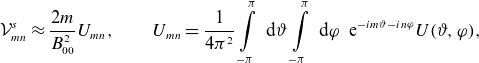 \begin{align} \mathcal{V}_{mn}^s\approx \frac {2 m}{B^2_{00}} U_{mn}, \qquad U_{mn} = \frac {1}{4\pi ^2}\int \limits _{-\pi }^{\pi }\textrm { d}\vartheta \int \limits _{-\pi }^{\pi }\textrm { d}\varphi \; \textrm { e}^{-im\vartheta -in\varphi } U(\vartheta, \varphi ), \end{align}
where coefficients $U_{mn}$
are real due to stellarator symmetry of
$U_{mn}$
are real due to stellarator symmetry of
 \begin{align} U(\vartheta, \varphi ) = \left ( \varepsilon _t\left (1-\cos \vartheta \right ) + \varepsilon _h\left (1-\cos \left (N_{\text{tor}}\varphi \right )\right ) \right )^{3/2}. \end{align}
Integrating in (A.2) by parts over both angles and explicitly computing the resulting second derivative $\partial ^2 U /(\partial \vartheta \partial \varphi )$
we present
$\partial ^2 U /(\partial \vartheta \partial \varphi )$
we present
 \begin{align} U_{mn}=\frac {3\varepsilon _t\varepsilon _h N_{\text{tor}}}{16 mn} \left ( W_{m+1,n+N_{\text{tor}}} + W_{m-1,n-N_{\text{tor}}} - W_{m+1,n-N_{\text{tor}}} - W_{m-1,n+N_{\text{tor}}} \right ), \end{align}
where coefficients
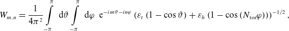 \begin{align} W_{m,n} = \frac {1}{4\pi ^2}\int \limits _{-\pi }^{\pi }\textrm { d}\vartheta \int \limits _{-\pi }^{\pi }\textrm { d}\varphi \; \textrm { e}^{-im\vartheta -in\varphi } \left ( \varepsilon _t\left (1-\cos \vartheta \right ) + \varepsilon _h\left (1-\cos \left (N_{\text{tor}}\varphi \right )\right ) \right )^{-1/2}, \end{align}
differ from zero for $n=k N_{\text {tor}}$
, where
$n=k N_{\text {tor}}$
, where $k$
is an integer. Reducing the integration over
$k$
is an integer. Reducing the integration over $\varphi$
for such
$\varphi$
for such $n$
to a single field period, expanding in the sub-integrand
$n$
to a single field period, expanding in the sub-integrand $(1-\cos \vartheta ) \approx \vartheta ^2/2$
and
$(1-\cos \vartheta ) \approx \vartheta ^2/2$
and $1-\cos \left (N_{\text{tor}}\varphi \right ) \approx N_{\text{tor}}^2\varphi ^2/2$
and then extending the integration over both angles to the infinite limits, which is justified for large
$1-\cos \left (N_{\text{tor}}\varphi \right ) \approx N_{\text{tor}}^2\varphi ^2/2$
and then extending the integration over both angles to the infinite limits, which is justified for large $m$
and
$m$
and $n$
, we get
$n$
, we get
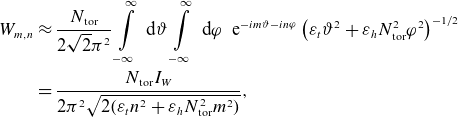 \begin{eqnarray} W_{m,n} \;&\approx &\; \frac {N_{\text{tor}}}{2\sqrt {2}\pi ^2} \int \limits _{-\infty }^{\infty }\textrm { d}\vartheta \int \limits _{-\infty }^{\infty }\textrm { d}\varphi \; \textrm { e}^{-im\vartheta -in\varphi } \left ( \varepsilon _t\vartheta ^2 + \varepsilon _h N_{\text{tor}}^2\varphi ^2 \right )^{-1/2} \nonumber \\ &=&\; \frac {N_{\text{tor}} I_W}{2\pi ^2\sqrt {2(\varepsilon _t n^2 + \varepsilon _h N_{\text{tor}}^2 m^2)}}, \end{eqnarray}
where we changed the integration variables from $(\vartheta, \varphi )$
to polar variables
$(\vartheta, \varphi )$
to polar variables $(\rho, \phi )$
as follows:
$(\rho, \phi )$
as follows:
 \begin{align} \vartheta = \left (m^2+\frac {n^2 \varepsilon _t}{\varepsilon _h N_{\text{tor}}^2}\right )^{-1/2}\rho \cos \phi, \qquad \varphi = \left (n^2+\frac {m^2 \varepsilon _h N_{\text{tor}}^2}{\varepsilon _t}\right )^{-1/2}\rho \sin \phi, \end{align}
in order to get
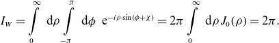 \begin{align} I_W = \int \limits _0^{\infty }\textrm { d} \rho \int \limits _{-\pi }^{\pi }\textrm { d}\phi \; \textrm { e}^{-i\rho \sin (\phi +\chi )} = 2\pi \int \limits _0^{\infty }\textrm { d} \rho J_0(\rho ) =2\pi . \end{align}
Here, $\chi = \text {atan}\left ((\varepsilon _h/\varepsilon _t)^{1/2}m N_{\text {tor}}/n\right )$
and
$\chi = \text {atan}\left ((\varepsilon _h/\varepsilon _t)^{1/2}m N_{\text {tor}}/n\right )$
and $J_0(\rho )$
is Bessel function of the first kind. For large
$J_0(\rho )$
is Bessel function of the first kind. For large $m$
and
$m$
and $n$
finite differences in (A.4) can be approximated by derivatives
$n$
finite differences in (A.4) can be approximated by derivatives
 \begin{align} U_{mn} \approx \frac {3\varepsilon _t\varepsilon _h N_{\text{tor}}^2}{4 mn} \frac {\partial ^2}{\partial m\partial n}W_{m,n} \approx \frac {9 \varepsilon _t^2 \varepsilon _h^2 N_{\text{tor}}^5} {4\pi \sqrt {2}\left (\varepsilon _t n^2 + \varepsilon _h N_{\text{tor}}^2 m^2\right )^{5/2}}. \end{align}
Expressing here modulation amplitudes via second derivatives of the field at the global maximum
 \begin{align} \varepsilon _t = - \frac {1}{B_{00}} \frac {\partial ^2 B}{\partial \vartheta ^2}, \qquad \varepsilon _h N_{\text{tor}}^2 = -\frac {1}{B_{00}} \frac {\partial ^2 B}{\partial \varphi ^2} = - \frac {1}{\beta B_{00}} \frac {\partial ^2 B}{\partial \vartheta ^2},\end{align}
where $\beta$
is defined in (4.1) and approximating
$\beta$
is defined in (4.1) and approximating $\eta _b \approx 1/B_{00}$
we present (A.9) as
$\eta _b \approx 1/B_{00}$
we present (A.9) as
 \begin{align} U_{mn} \approx \frac {9\beta ^{1/2}\eta _b^{3/2}}{4\pi \sqrt {2}}\left |\frac {\partial ^2 B}{\partial \vartheta ^2}\right |^{3/2} \frac {N_{\text {tor}}}{\left (m^2+\beta n^2\right )^{5/2}} \end{align}
which, together with $\eta _b \approx 1/B_{00}$
in the first (A.2), results in (4.11).
$\eta _b \approx 1/B_{00}$
in the first (A.2), results in (4.11).


 Open access