


1. Introduction
The Andes of north-central Chile (or Norte Chico) are characterised by elevations up to 6000 m above sea level (a.s.l.), low humidity and intense solar radiation (Favier and others, Reference Favier, Falvey, Rabatel, Praderio and López2009; MacDonell and others, Reference MacDonell, Kinnard, Mölg, Nicholson and Abermann2013; Lhermitte and others, Reference Lhermitte, Abermann and Kinnard2014). The region extends along the western side of the Andes Cordillera between the southern edge of the Atacama Desert (26° S) and the Aconcagua River basin (33° S). Precipitation in the low-lying valleys is low, increasing from north to south from ∼50 to 300 mm a−1, falling mostly during the winter season (Favier and others, Reference Favier, Falvey, Rabatel, Praderio and López2009) and as snow above ∼2500 m a.s.l. (Schauwecker and others, Reference Schauwecker, Palma, MacDonell, Ayala and Viale2022). There are numerous glaciers and rock glaciers above 3500 m a.s.l., with rock glaciers dominating until 4800 m a.s.l. and debris-free glaciers above that elevation (Barcaza and others, Reference Barcaza2017; DGA, 2022). In the classification proposed by Lliboutry (Reference Lliboutry1998), the glaciers of north-central Chile are located at the edge between the Desert and the Central Andes, both forming what is referred to as the Dry Andes (Barcaza and others, Reference Barcaza2017; Dussaillant and others, Reference Dussaillant2019). Glaciers in these regions have been thinning and retreating over the last century (Masiokas and others, Reference Masiokas2020), with an increasingly negative mass balance in the last two decades (Dussaillant and others, Reference Dussaillant2019; Hugonnet and others, Reference Hugonnet2021). As north-central Chile depends on snow and ice meltwater for agriculture, human consumption, industry and ecosystems (Cortés and others, Reference Cortés2012; Valois and others, Reference Valois, MacDonell, Núñez Cobo and Maureira-Cortés2020; Navarro and others, Reference Navarro, Valois, MacDonell, de Pasquale G and Díaz2023b), the monitoring of the snow cover and glaciers is essential to quantify and project water availability, especially during droughts, and understand changes in precipitation and temperature (Favier and others, Reference Favier, Falvey, Rabatel, Praderio and López2009; Yáñez San Francisco and others, Reference Yáñez San Francisco, Aguilar and MacDonell2023).
Since 2010, central Chile has been affected by a severe drought with average precipitation deficits of 20–40% extending from ∼29° S to 40° S (Garreaud and others, Reference Garreaud2017; Garreaud and others, Reference Garreaud, Boisier, Rondanelli, Montecinos, Sepúlveda and Veloso-Aguila2020). The drought has been termed the Chilean Megadrought and is unprecedented in severity, duration and spatial extent, with cascading effects on vegetation, streamflow levels, wildfires and glacier mass balance (e.g. Garreaud and others, Reference Garreaud2017; Dussaillant and others, Reference Dussaillant2019; McCarthy and others, Reference McCarthy2022). The causes of the Megadrought lie in a particular configuration of the Pacific Ocean driven by a combination of natural variability and anthropogenic forcing (Garreaud and others, Reference Garreaud, Boisier, Rondanelli, Montecinos, Sepúlveda and Veloso-Aguila2020). Climate projections for north-central Chile indicate a decrease in precipitation of up to 40% and an increase in air temperature of up to 5°C by the end of the century under high greenhouse gas emission scenarios (SSP5-8.5) (Salazar and others, Reference Salazar, Thatcher, Goubanova, Bernal, Gutiérrez and Squeo2024). Consequently, mountain water resources are expected to be severely affected by these changes, threatening water security in adjacent lowland areas.
In this study, we focus on Tapado Glacier (30.1422° S, 69.9275° W), a 1.5 km2 glacier located on the southern slope of Cerro Tapado (5536 m a.s.l.), ranging in elevation from ∼4515 to 5535 m a.s.l. The Tapado Glacier is the fifth largest glacier in north-central Chile (DGA, 2022) and has been the focus of several previous studies and monitoring efforts (e.g. CEAZA, 2010, 2015, 2023). The glacier contains several types of surfaces and features, such as supraglacial ponds and ice cliffs over a debris-covered section, a field of large snow and ice penitentes, an icefall with crevasses and seracs and wind-exposed upper areas with little snow accumulation and melt. The ablation and evolution of these features are driven by different processes, such as complex snow accumulation patterns (Réveillet and others, Reference Réveillet, MacDonell, Gascoin, Kinnard, Lhermitte and Schaffer2020; Ayala and others, Reference Ayala, Schauwecker and MacDonell2023), spatially heterogeneous ablation and energy fluxes (Lhermitte and others, Reference Lhermitte, Abermann and Kinnard2014; Sinclair and MacDonell, Reference Sinclair and MacDonell2016) and water production and transfer through several cryo-hydrological compartments, including a thermokarst drainage network and a glacial foreland (Pourrier and others, Reference Pourrier, Jourde, Kinnard, Gascoin and Monnier2014; Navarro and others, Reference Navarro, MacDonell and Valois2023a). The diversity of processes makes Tapado Glacier an ideal test site for understanding how surface type impacts ablation rates, and the physical processes driving glacier mass loss and their impact on hydrology and water resources in semiarid catchments.
The magnitude and relative importance of the processes controlling the mass balance of Tapado Glacier is unknown, mainly due to the lack of specific and quantitative information. In our study, we address this knowledge gap by taking advantage of a compilation of field and remotely sensed datasets to (i) describe and quantify the physical processes driving the mass loss of Tapado Glacier and (ii) compare mass loss rates from previous decades with more recent years, which were obtained during a particularly dry period. Datasets include meteorological data, ablation stake readings, photographs from automatic cameras, Light Detection and Ranging (LiDAR) and Uncrewed Aerial Vehicle (UAV) surveys and satellite products. We expect that our results will shed light on the dynamics of glacier mass loss in the Dry Andes and other arid and semi-arid regions around the world.
2. Study site and relevant processes
Tapado Glacier is located in the upper Elqui River basin (La Laguna basin), east of the city of La Serena in the Coquimbo region, north-central Chile (Fig. 1a). The glacier has an area of 1.5 km2 and consists of a debris-free and a debris-covered section (Fig. 1b and c). The equilibrium line altitude has previously been estimated at ∼5300 m a.s.l. (Kull and others, Reference Kull, Grosjean and Veit2002). The debris-free section has a southerly orientation and extends from the summit of Cerro Tapado (5536 m a.s.l.) to the foot of a glacial cirque at 4600 m a.s.l. It is composed of a dome at the top from which it flows down a steep slope resulting in crevassed areas. Below the glacier dome (at ∼5000 m a.s.l.), a steep area of exposed bedrock partially disrupts the ice flow in the eastern sector of the debris-free glacier, generating a marginal ice cliff 10–20 m tall, from which frequent falls of snow and ice occur. The lower areas of the debris-free section comprise a less steep plateau covered by large ice penitentes (2–3 m), which ends abruptly at a steep edge (CEAZA, 2012). The western section develops into a debris-covered area characterised by a low slope and a rugged surface due to the presence of numerous ice cliffs and supraglacial ponds (Monnier and others, Reference Monnier, Kinnard, Surazakov and Bossy2014). The altitudinal distribution of debris-free and debris-covered areas can be observed in Figure 2. In its terminal part, the debris-covered section is in contact with a rock glacier system with at least four distinct units (Vivero and others, Reference Vivero2021). The group of landforms formed by Tapado Glacier and the surrounding rock glaciers is also referred to as Tapado Glacier complex (Monnier and others, Reference Monnier, Kinnard, Surazakov and Bossy2014; Schaffer and others, Reference Schaffer, MacDonell, Réveillet, Yáñez and Valois2019). Helicopter-borne radar soundings have estimated a maximum ice thickness of 69 m and a total ice volume of 57 × 106 m3 for the debris-free and debris-covered sections (Geoestudios, 2014). Tapado Glacier lost 25.2% of its area between 1956 and 2020 and its mass balance has become increasingly more negative since the year 2000 (Robson and others, Reference Robson, MacDonell, Ayala, Bolch, Nielsen and Vivero2022).
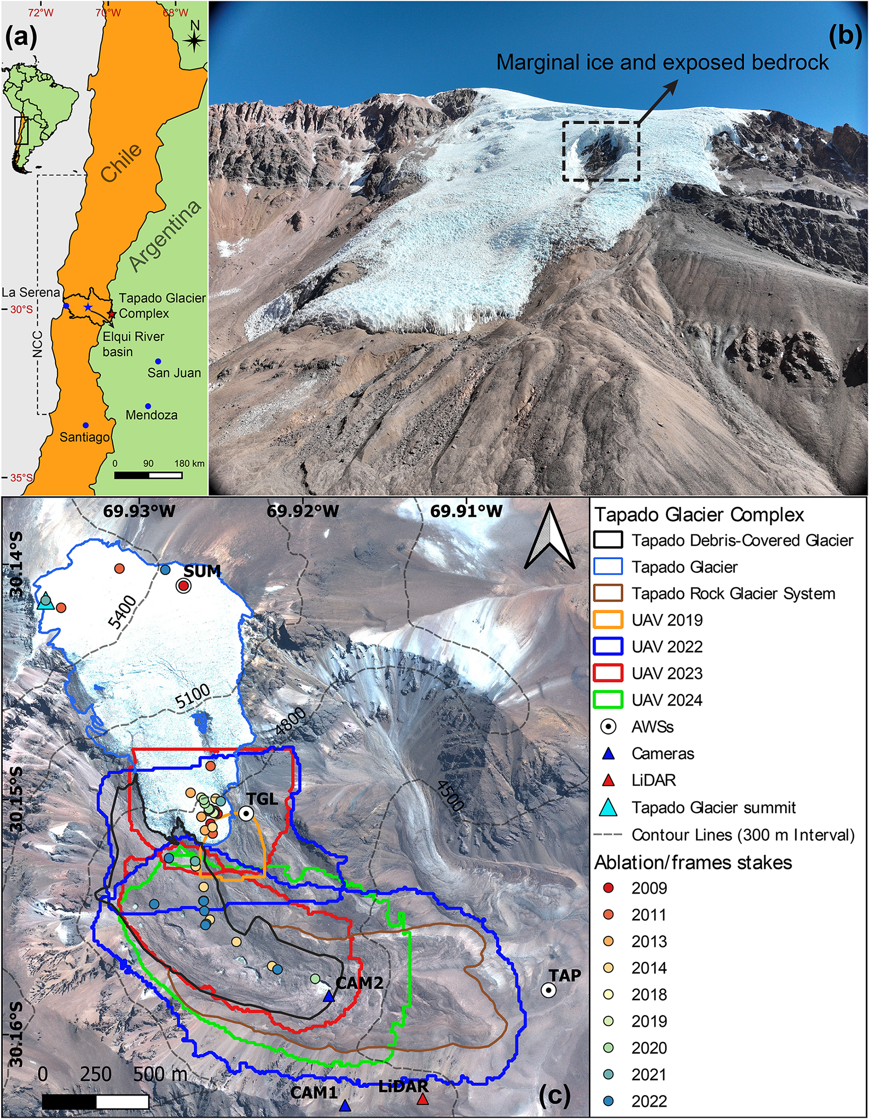
Figure 1. (a) Tapado Glacier in South America and north-central Chile (NCC), (b) Tapado Glacier in summer 2023 (UAV image by Gonzalo Navarro), (c) Tapado glacier complex including Tapado Glacier (debris-free and debris-covered sections) and Tapado rock glacier system. Glacier outlines are delimited based on Robson and others (Reference Robson, MacDonell, Ayala, Bolch, Nielsen and Vivero2022) and using a Pléiades satellite image from March 2020. Field data, including ablation stakes, automatic cameras, meteorological stations and areas surveyed by UAV flights in 2019, 2023 and 2024 are shown.
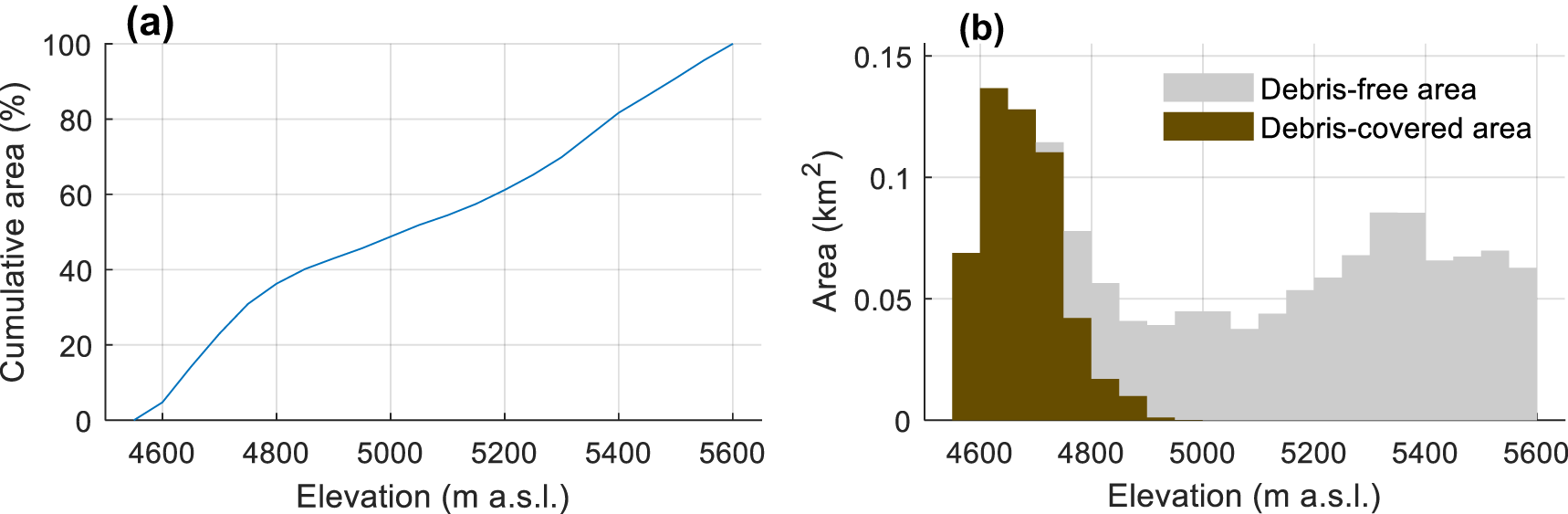
Figure 2. (a) Glacier hypsometry, (b) Altitudinal distribution of glacier debris-free and debris-covered areas. The elevation data correspond to a 2020 DEM derived from Pléiades imagery (see Section 3.3.2).
One of the key processes shaping the mass balance of Tapado Glacier is the interplay between sublimation and melt. Ginot and others (Reference Ginot, Kull, Schotterer, Schwikowski and Gäggeler2006) used chemical records from a 36 m long ice core extracted from the summit of Cerro Tapado (5536 m a.s.l.) to reconstruct glacier mass balance in the period 1962–99. They estimated an average annual net accumulation of 316 mm w.e., with ablation being dominated by sublimation (327 mm w.e. a−1). Melting was less important and varied between 8 and 122 mm w.e. a−1. Subsequent studies have estimated summer sublimation rates varying between 0.6 and 5 mm d−1 over the debris-free section of the glacier using energy balance models forced by in situ meteorological data (CEAZA, 2010, 2012; Ayala and others, Reference Ayala, Pellicciotti, MacDonell, McPhee and Burlando2017; Yáñez San Francisco and others, Reference San Francisco E, MacDonell and Casassa2025). Using distributed snow modelling, Réveillet and others (Reference Réveillet, MacDonell, Gascoin, Kinnard, Lhermitte and Schaffer2020) calculated that sublimation represents more than 50% of the total ablation in the La Laguna basin, while Ayala and others (Reference Ayala, Schauwecker and MacDonell2023) proposed that snowmelt is limited to areas with specific topographic and meteorological conditions that allow large snow accumulation and limited snow removal. Over the debris-free section of Tapado Glacier, the role of the winter snow cover is crucial, protecting the ice surface from the intense solar radiation. Once the snow disappears, the ice melting rates can reach values up to 30 mm w.e. d−1 (Ayala and others, Reference Ayala, Pellicciotti, MacDonell, McPhee and Burlando2017).
Penitentes are one of the most striking consequences of the interplay between sublimation and melt (Nicholson and others, Reference Nicholson, Pȩtlicki, Partan and MacDonell2016; Sinclair and MacDonell, Reference Sinclair and MacDonell2016). Penitentes are spikes of snow and ice formed by differential ablation; while sublimation dominates at their peaks, melt and enhanced ablation occur in the confined troughs between them (Lliboutry, Reference Lliboutry1954; Corripio and others, Reference Corripio, Purves, Rivera, Orlove, Wiegandt and Luckman2008). Penitentes can reach heights of more than 3 m on the tongue of the debris-free section of Tapado Glacier (see Fig. S1). Several studies have investigated different aspects of the penitentes of Tapado Glacier, including their shapes (Nicholson and others, Reference Nicholson, Pȩtlicki, Partan and MacDonell2016), effect on surface albedo measurements (Lhermitte and others, Reference Lhermitte, Abermann and Kinnard2014) and impact on ablation processes (Sinclair and MacDonell, Reference Sinclair and MacDonell2016).
The surface of the debris-covered section of Tapado Glacier exhibits thermokarst depressions, supraglacial ponds, massive ice exposures, closed cracks and chaotic hummocky terrain (Monnier and others, Reference Monnier, Kinnard, Surazakov and Bossy2014; Pourrier and others, Reference Pourrier, Jourde, Kinnard, Gascoin and Monnier2014; Vivero and others, Reference Vivero2021). It has been shown that due to the insulating effect of debris, most ice ablation on debris-covered glaciers occurs at ice cliffs and supraglacial ponds, where the ice is exposed to the atmosphere and the ponds act as recipients of energy that are then transferred to the glacier system (e.g. Miles and others, Reference Miles, Pellicciotti, Willis, Steiner, Buri and Arnold2016). On Tapado Glacier, meltwater from cliffs and ponds percolates to the internal structure of the debris-covered glacier, where it mixes with meltwater from the upper debris-free section and is transferred to a downslope rock glacier through a complex structure of englacial conduits to emerge at a spring in a lower moraine (Pourrier and others, Reference Pourrier, Jourde, Kinnard, Gascoin and Monnier2014; Navarro and others, Reference Navarro, MacDonell and Valois2023a).
3. Data and methods
3.1. Meteorological data
Table 1 presents a summary of the Automatic Weather Stations (AWSs) and the monitored variables that are used in this study. The AWS with the longest record is La Laguna DGA (LAG_DGA), located 13 km west of the glacier, which is operated by the National Water Directory (Dirección General de Aguas, DGA). The other AWSs were installed after 2009, provide hourly data and are maintained by CEAZA (www.ceazamet.cl). Three stations located near or on Tapado Glacier are shown in Figure 1c (SUM, TGL and TAP). Details about SUM and TGL can be found at CEAZA (2012) and Ayala and others (Reference Ayala, Schauwecker and MacDonell2023), respectively.
Table 1. Meteorological stations and variables used in this study. For more details see www.ceazamet.cl. Data from LAG_DGA can be accessed at dga.Mop.Gob.Cl
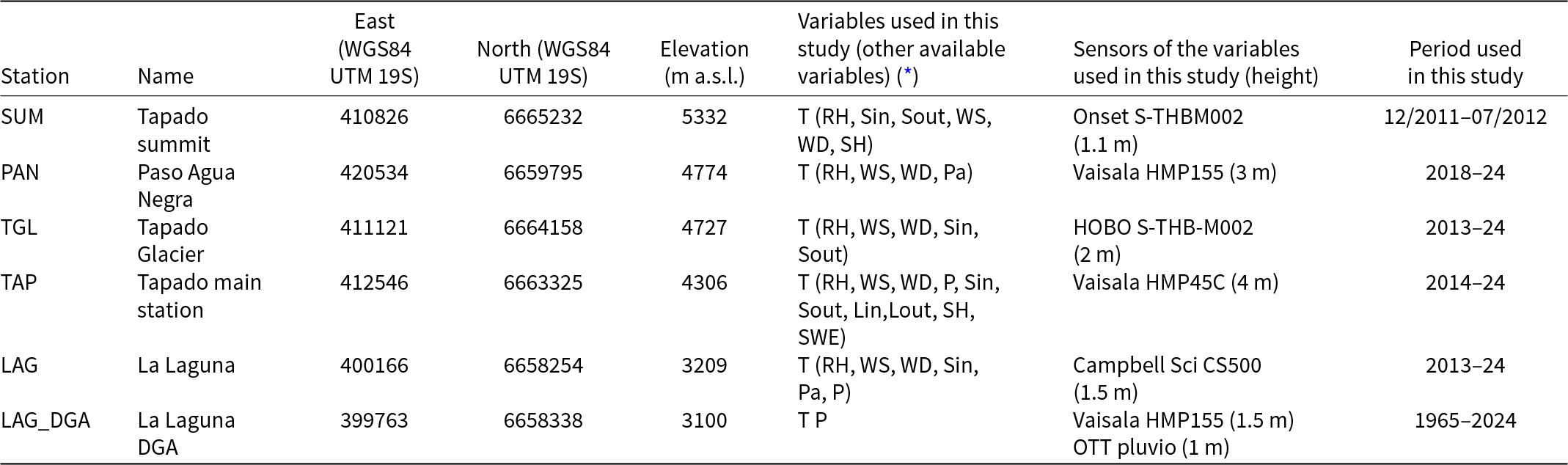
* T: Air temperature, P: Precipitation, RH: Relative humidity, Sin: Incoming shortwave radiation, Sout: Reflected shortwave radiation, WS: Wind speed, WD: Wind direction, Pa: Air pressure, Lin: Incoming longwave radiation, Lout: Outgoing longwave radiation, SH: Snow height, SWE: Snow water equivalent.
In this study, we use precipitation and air temperature records from LAG_DGA to estimate changes and trends in precipitation during the accumulation season (considered here as April to October) and annual mean air temperature during the period 1965–2024. Summer (DJF) mean air temperatures at LAG_DGA and a temperature lapse rate calculated from the remaining stations are used to estimate changes in the summer 0°C isotherm altitude for the period 1974–2024. The trend analysis is carried out using Mann–Kendall and Sen’s slope.
3.2. Field data
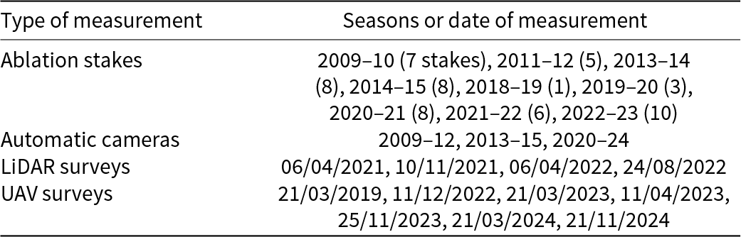
Several glaciological studies have been carried out on Tapado Glacier since 2009 (Table 2) (CEAZA, 2010, 2012, 2015). The data collected range from point-scale direct measurements of winter snow accumulation and ablation to terrestrial LIDAR and UAV surveys. This section summarises the main characteristics of the data collected.
Table 2. Summary of field data collected at Tapado Glacier and presented in this study. See Figure 1 for position of measurements
3.2.1. Direct surface measurements
Direct surface measurements consist of manual readings of ablation stakes drilled into debris-free or debris-covered ice (CEAZA, 2010, 2012, 2015; Ayala and others, Reference Ayala, Schauwecker and MacDonell2023). To account for changes in the irregular terrain defined by the penitentes field, some of the ablation measurements were made using ablation frames. An ablation frame is a 3–4 m horizontal aluminium pipe supported by two vertical tubes drilled into the surface (Nicholson and others, Reference Nicholson, Pȩtlicki, Partan and MacDonell2016). The distance from the horizontal pipe to the glacier surface is then measured every 10–20 cm. In addition, direct measurements of the height of individual penitentes were performed for a few penitentes using snow probes (from one to three measurements per season). In this study, we use the ablation stakes data to calculate cumulative ablation and ablation rates in different glacier sections.
3.2.2. Automatic cameras
In November 2009, an automatic camera focused on the debris-free glacier was placed on a ridge located 1.5 km southeast of Tapado Glacier (CAM1 in Fig. 1c) (CEAZA, 2012). The setup consisted of a Harbortronics autonomous time-lapse camera package containing a CANON EOS digital Rebel XS camera (22.2 × 14.8 mm sensor dimensions), Digisnap electronic trigger, lithium battery and 12-volt solar panel. The camera captured from one to three daily images in the period November 2009 and April 2012 between 10:00 and 14:00 hours. The pictures were stored as CR2 files. This installation was repeated between November 2013 and April 2015 (CEAZA, 2012; Vivero, Reference Vivero2024). After the removal of the camera, a new camera with the same configuration was placed on the debris-covered Tapado Glacier facing the debris-free section and a supraglacial pond (CAM2 in Fig. 1c). In this third collection, the camera captured daily pictures of Tapado Glacier at midday between February 2020 and April 2024. In our study, we use the images taken by the automatic cameras to monitor snowfall and icefall events from the marginal ice surrounding an area of steep exposed bedrock in the debris-free section. We individually examine the pictures in each ablation period (November–April) and register the ones that show evidence of snowfall, icefall or rockfall.
3.2.3. LiDAR surveys
In 2021 and 2022, a total of four terrestrial LiDAR surveys were carried out using a RIEGL VZ-6000 device. This device has a measuring range of up to 6 km and operates at a wavelength of 905 nm, which means the signal avoids absorption by snow or ice surfaces (Prokop, Reference Prokop2008; RIEGL Laser Measurement Systems, 2015). LiDAR point cloud acquisition is a precise technique for obtaining digital terrain models that are often used in cryospheric studies (Buckley and others, Reference Buckley, Schwarz, Terlaky, Howell, Arnott, Bretar, Pierrot-Deseilligny and Vosselman2009). To minimise errors in data acquisition and post-processing, we generated a local reference frame by establishing a joint measurement system between laser scans and Global Navigation Satellite System (GNSS) control points. LiDAR measurements were performed at a frequency of 30 kHz, a vertical angle range of 60° to 120°, a horizontal scan of ∼90° to 210° and a vertical and horizontal angular step resolution of 0.012°. The collected data were processed with the RISCAN PRO software.
The LiDAR surveys were made from a ridge located on the southern basin divide at an approximate distance of 2 km, in front of Tapado Glacier (Fig. 1c). The positioning and alignment of the LiDAR measurements were achieved using three control points corrected by a GNSS base and through the differentiation and adjustment of common stable areas. The surveys resulted in digital elevation models (DEM) of 1 m spatial resolution.
3.2.4. UAV surveys
A set of UAV surveys were carried out over different sections of Tapado Glacier during the period 2019–24 (Fig. 1c and Table 2). In this study, we use the data collected over the lower part of the debris-free section to calculate changes in the elevation of the surface and the size of the snow and ice penitentes (Section 3.3.2). Additionally, the 2023 and 2024 images are used to delineate ice cliffs and supraglacial ponds over the debris-covered glacier (Section 3.3.1).
Tapado penitentes were first surveyed on 21 March 2019 from 12:30 to 13:00 local time. The date and time of the survey provided optimal optical conditions for observing the penitentes from above, with almost no shadows due to the configuration of the sun angle with respect to the geometry of the penitentes. The 2019 survey was carried out using a DJI Phantom 4 Pro quadcopter UAV, which is equipped with a standard single-frequency GNSS system for metric precision positioning. The camera has a resolution of 12.4 MP and an image size of 5472 × 3078 pixels. The flight plan was carried out using PiX4Dcapture with a double grid pattern and a height above take-off of 45 m. The images were collected with a longitudinal and lateral overlap of 75%. The survey consisted of 210 nadir images and covered an area of 0.08 km2 located on the eastern part of the debris-free section.
A DJI Mavic 3E was used for the rest of the surveys, using a 20 MP camera and an image size of 5280 × 3956. The UAV was flown with an 80% latitudinal and longitudinal overlap at a flying height of 60 m above the terrain (based on a 2020 Pléiades DEM of the area), planned and deployed using the DJI Pilot 2 software installed on a DJI Remote Controller Pro. The UAV was equipped with a Real Time Kinematics (RTK) module connected to a DJI RTK Base station which allowed the position of the photographs to be recorded with accuracies of 1.1 cm (horizontal) and 2.6 cm (vertical), relative to the DJI D-RTK 2 mobile station location.
UAV images were processed using Pix4Dmapper commercial software for automatic keypoint feature detection, image matching and fusion using SfM algorithms (Westoby and others, Reference Westoby, Brasington, Glasser, Hambrey and Reynolds2012; Smith and others, Reference Smith, Carrivick and Quincey2016). The initial keypoint processing was performed at full image scale and using an aerial grid model with geometrically verified matching. Camera calibration of internal parameters was performed automatically. Subsequently, we performed a point cloud densification using half image scale with three as the minimum number of matches for each point. From these results, we generated 3D meshes (see Data Availability for data and visualisation) and high-resolution DSM and orthomosaics with a resolution of 2 cm.
The raw point clouds from 2019, 2023 and 2024 were then processed in Pix4Dsurvey to extract the peaks and troughs of the penitentes, similar to estimating tree height from dense point clouds (Zeybek and Şanlıoğlu, Reference Zeybek and Şanlıoğlu İ2019). This procedure includes an initial distant outlier filter and a terrain filter to extract the penitentes from the surrounding bare ground. For this, a ground height threshold of 0.5 m and a sampling distance on the irregular surface of 1.5 m was applied. After the subsequent masking, we applied a low-pass filter to the area covered by the penitentes to segment the trough and tip of each penitente (Fig. S2). The point clouds were analysed in a 2.25 m2 grid and the vertical difference between the tips and troughs of the penitentes was determined.
3.3. Satellite and aerial products
3.3.1. Glacier and supraglacial ponds and ice cliffs delineation
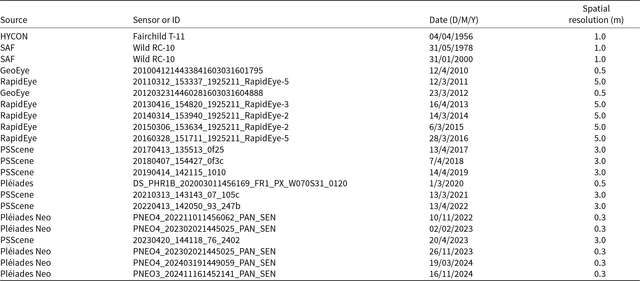
We determine changes in the extent of Tapado Glacier over the period 1956–2024 using a set of satellite and aerial images. Each image was acquired at the end of the austral summer (February–April) and has a spatial resolution of at least 5 m (Table 3). We selected images with the minimum presence of snow, clouds and shadows. Glacier outlines were manually delineated for the debris-free section using the 1956, 1978 and 2000 aerial images and the 2012 GeoEye satellite image. For the remaining images, we used a semi-automated approach based on the ratio of image spectral bands. Previous studies have demonstrated that the red and shortwave infrared (SWIR) bands can be used to map snow and ice (e.g. Paul and others, Reference Paul, Winsvold, Kääb, Nagler and Schwaizer2016). However, as the SWIR bands were not available in all the images in our study, we used the normalised difference water index (NDWI), which is based on the normalised ratio between the green (B_green) and near-infrared (B_NIR) bands. This approach also provides a clear signal for snow and ice areas (e.g. Korzeniowska and others, Reference Korzeniowska, Bühler, Marty and Korup2017), but it does not distinguish between liquid and frozen water, and it can be affected by shadows (Miles and others, Reference Miles, Willis, Arnold, Steiner and Pellicciotti2017). The equation used for the glacier delineation is shown in Equation 1 (Dozier, Reference Dozier1989; McFeeters, Reference McFeeters1996):
 \begin{equation}{\text{NDWI = }}\left( {{\text{B\_green }} - {\text{ B\_NIR}}} \right){\text{/}}\left( {{\text{B\_green + B\_NIR}}} \right)\end{equation}
Table 3. Satellite and aerial images used for glacier and supraglacial ponds and ice cliffs delineation
For each year, we defined a threshold value that distinguishes between a snow or ice surface and bare ground (or debris-covered areas) based on the comparison with the previous and next images and a visual inspection of the true colour image. Changes of <2 pixels between two successive images were not mapped because they were within the error range of the method. Ephemeral snow patches on the upper areas were excluded from the glacier outlines and only became part of the glacier if they persisted for a period of at least 5 years. The error in the values for the glacier area was estimated using the buffer method by Paul (Reference Paul2017). The extent of the debris-covered section and the Tapado rock glacier were delineated using the 2020 Pléiades image. As the changes in the debris-covered lowest boundaries since 1956 have been relatively small, we maintained these boundaries throughout the study period. In contrast, the upper areas of the debris-covered section were re-delineated for 1956, 1978, 2000, 2020 and 2024, accounting for the changes of the debris-free section. The error in the surface area of the debris-covered section is estimated as 5% of the delineated area. In addition, the 2012 image was used to delineate the area covered by the ice penitentes in the lower part of the debris-free section.
The historical set of satellite, aerial and UAV images was also used to manually delineate the ice cliffs and supraglacial ponds over the debris-covered section of Tapado Glacier. For this, we selected six images with the best resolution, colour and contrast available from our dataset. The selected images correspond to the years 2000, 2010, 2012, 2020, 2023 and 2024 (see Table 3). Due to its insufficient contrast, the image of 2000 was used only to map the ponds, but not the ice cliffs. The identification and delimitation of the ponds and cliffs were more difficult in the aerial and satellite images of 2000, 2010 and 2012 compared to the images captured by the UAV flights in 2023 and 2024, which had a very high spatial resolution and quality. Due to these differences, we set a minimum size of 40 m2 for our temporal analysis, as ponds and cliffs below this threshold cannot be delimited with confidence in the older images. We verified that the ponds and cliffs with areas smaller than 40 m2 correspond to <10% of the total pond and cliff area identified in the UAV images. We use the delineation of cliffs and ponds to define the total area where these features have developed in the 2012–24 period. This area was obtained by merging all the available outlines and adding a buffer of 10 m.
3.3.2. Geodetic mass balance and volumetric changes
LiDAR, UAV and tri-stereo satellite imagery (Pléiades and Pléiades Neo) were used for the calculation of DEMs of Difference (DoDs) in the period 2020–24. The LiDAR datasets were provided as gridded rasters at 1 m resolution. The processing of the UAV datasets is described in Section 3.2.3. The satellite imagery was photogrammetrically processed using Catalyst Professional (formally known as PCI Geomatica). Initially, the DEM for the year 2020 was created utilising the rational polynomial coefficients (RPCs) that came with the satellite images. Automatic tie-points were used to solve the relative orientation and perform a bundle adjustment. Subsequently, epipolar images were created, which were used for the extraction of the DEM at a 1 m resolution employing a semi-global matching algorithm. This particular algorithm is recognised for its superiority over normalised cross-correlation (NCC) methods, resulting in cleaner DEMs (Hirschmuller, Reference Hirschmuller2008). The extracted DEM was then used to orthorectify the satellite images and produce an orthomosaic. This methodology was replicated for the subsequent datasets, using the 2020 orthomosaic and DEM as reference surfaces for automatic ground control point location to ensure maximal alignment of the datasets.
Small planimetric co-registration biases were apparent between the different DEM products, as such the co-registration method set out by Nuth and Kääb (Reference Nuth and Kääb2011) was implemented. This method minimises the root mean square slope normalised elevation biases over stable terrain in order to solve co-registration biases between DEMs. It was implemented using the xDEM python package (https://github.com/GlacioHack/xdem). The co-registered DEM pairs were then used to determine both surface elevation changes as well as geodetic mass balance. The latter requires a volume-to-mass conversion factor, which for the ablation season was assumed to be 850 ± 60 kg m−3 (Huss, Reference Huss2013), while for the accumulation period, we used a snow density value of 460 kg m−3, which is the average of several end-of-winter snow pits dug between 2021 and 2023. Given the spatial and temporal variability of snow density throughout the accumulation season, we used an uncertainty of ±120 kg m−3 for each winter balance.
The uncertainty in glacier elevation change was estimated following the methodology of Hugonnet and others (Reference Hugonnet2022), implemented in the xDEM package. This approach accounts for heteroscedasticity (i.e. the variability of elevation errors depending on terrain characteristics) and spatial correlations of errors. Spatial autocorrelation of elevation errors was quantified using empirical variograms derived from stable terrain, which served as a proxy for error structure. Terrain slope and curvature were used as explanatory variables to model the elevation-dependent variability of errors. This resulted in gridded estimates of the uncertainty in the elevation change. The propagated uncertainties were estimated using spatial error propagation, following Hugonnet and others (Reference Hugonnet2022), which accounts for both the heteroscedasticity and spatial correlation of errors. The uncertainty in the geodetic mass balance was then calculated as the root sum of squares of the elevation change error, the assumed uncertainty in the density conversion and a 5% uncertainty in the glacier area, following Farías-Barahona and others (Reference Farías-Barahona2019).
To contrast the recent changes in Tapado Glacier with those reported for previous decades, our analysis included the maps of elevation changes obtained by Robson and others (Reference Robson, MacDonell, Ayala, Bolch, Nielsen and Vivero2022) for the periods 1956–78, 1978–2000, 2000–12, 2012–15, 2012–20 and 2015–20. The maps of elevation changes derived by Robson and others (Reference Robson, MacDonell, Ayala, Bolch, Nielsen and Vivero2022) and their associated uncertainty were clipped to our glacier outlines (Section 3.3.1). Elevation changes for all the periods were converted to mass balance using a density of 850 kg m−3. To account for glacier area changes in the calculation of the geodetic mass balance, the glacier total area is updated roughly every 20 years using the outlines delineated for 1956, 1978, 2000 and 2020.
3.3.3. Albedo changes of the debris-free section
We use the surface reflectance of the Landsat archive to estimate the minimum summer albedo of the debris-free section of Tapado Glacier from 1985. For this, we first homogenised the reflectance of L8 OLI to L7/L5 ETM (Roy and others, Reference Roy2016) for all the images covering the study area acquired between February and May in the period 1985–2024. A maximum of 25% cloud cover was tolerated within the images. Approximately 90% of all images had <10% cloud cover. We later applied a terrain correction to the reflectance (Soenen and others, Reference Soenen, Peddle and Coburn2005) and removed all the values outside the range between 0 and 1. Band reflectance is converted to broadband albedo (Knap and others, Reference Knap, Reijmer and Oerlemans1999). Green band saturation in L5/L7 was taken into account, when it occurs by using different transfer functions from Knap and others (Reference Knap, Reijmer and Oerlemans1999). A minimum albedo map was produced by calculating the minimum albedo at each pixel between February and May of each year. Finally, we obtained an albedo time series for the debris-free section by spatially averaging each annual minimum albedo map, using the outlines corresponding to the minimum extent of the debris-free section (end of summer 2024). The day of year (doy) on which the minimum albedo was extracted at each pixel was also spatially averaged and reported to assess its effect on albedo variability over time.
4. Results
4.1. Climate drivers
The LAG_DGA record shows that precipitation during the accumulation season averaged 133 mm a−1 over the period 1965–2023, with a median value of 102 mm a−1 (Fig. 3a). We observe a relatively large interannual variability of precipitation (coefficient of variation of 1.06) and frequent droughts with periods of almost zero precipitation. Given this large interannual variability, it is difficult to identify a trend in precipitation. Before the onset of the Chilean Megadrought in 2010, we identify two periods of below-average winter precipitation before the year 2000 (1966–74 and 1988–96). Since 2010, winter precipitation has been 43% lower than the 1965–2009 average. Austral winters with more than 300 mm a−1 of precipitation have not been observed since 2002, and summer precipitation is mostly negligible. Since 2009, we identify two extended periods of below-average precipitation, 2009–14 and 2018–23. The dry period from 2009 to 2014 was followed by 3 years of near-average precipitation (2015–17). Although precipitation records at LAG_DGA also show a very dry winter in 2022, snow records at TAP show that snow accumulation in the surroundings of Tapado Glacier was close to average (Fig. S3).
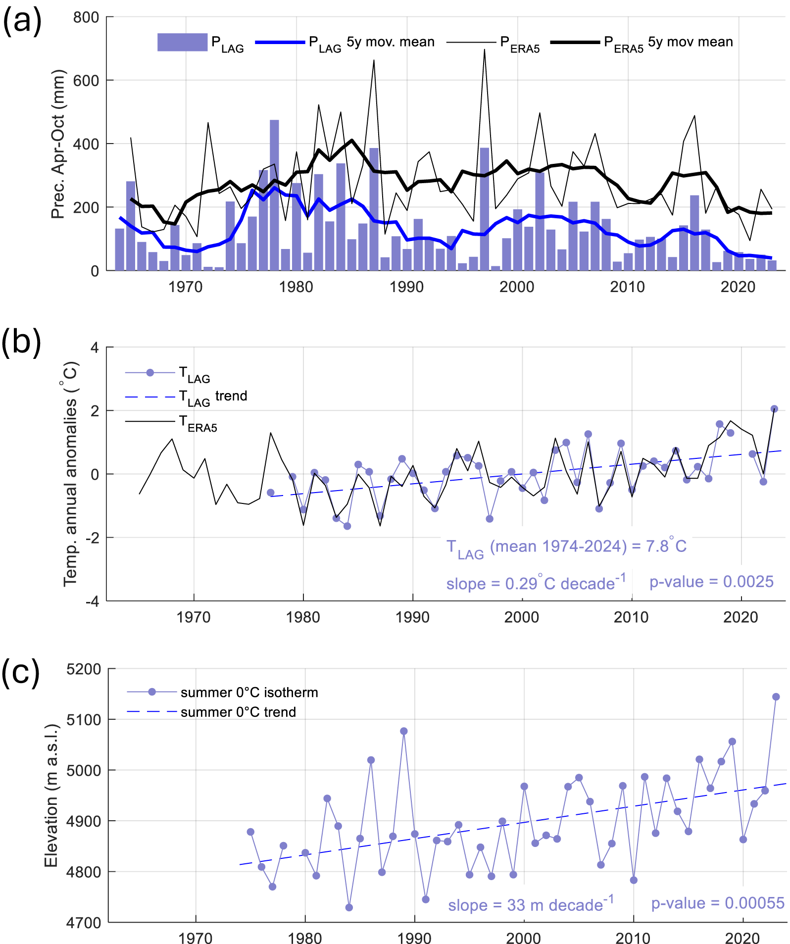
Figure 3. (a) Precipitation during the accumulation season (April to October) as measured by LAG_DGA and estimated by ERA5. (b) Anomaly of annual mean air temperatures at LAG_DGA and from ERA5. (c) Elevation of the summer 0°C isotherm in La Laguna river basin. We indicate the slope of the estimated linear trends at a significance level of 5% and its p-value.
We calculate an annual mean air temperature at LAG_DGA of 7.8°C for the period 1974–2024 with a significantly increasing trend of 0.29°C per decade (Sen’s slope and a Mann–Kendall p-value of 0.0025 at a 5% level), resulting in an increase of 1.5°C over the last 50 years (Fig. 3b). The results for the ERA5 data also show a significant positive trend (0.19°C per decade, 5% level, p-value = 0.0015). In the last decade, the years 2018 and 2023 have registered record-high annual air temperatures. We obtained an average austral summer (DJF) temperature lapse rate of 7.6 ± 0.4°C km−1 (average and interannual standard deviation) across the La Laguna basin. Using this value, we estimate that the summer average 0°C isotherm has significantly increased by 150 m since 1974 (33 m per decade, p-value = 0.00055, Fig. 3c).
4.2. Glacier ablation and mass balance
4.2.1. Direct measurements
We integrated the multi-annual glacier ablation measurements into a single dataset. Figure 4 shows the data organised into four glacier sections distributed along the elevation profile of the glacier: debris-covered, ice penitentes (divided into two elevation ranges: 4700–4770 and 4470–4880 m a.s.l.) and the upper debris-free areas (>4900 m a.s.l.). Results show that over each ablation season, the largest ablation occurred at the ice penitentes section, while lower ablation was measured at the debris-covered and upper debris-free areas (Fig. 4a–d). Similar results are obtained for the ablation rates, which vary from 0 to 30 mm w.e. d−1 in the debris-covered and upper debris-free areas to 10–70 mm w.e. d−1 at the ice penitentes section (Fig. 4e–h and j). As expected from studies in debris-covered glaciers (e.g. Östrem, Reference Östrem1959; Evatt and others, Reference Evatt2015), mid-summer ice ablation rates under debris show an inverse relationship to debris thickness (Fig. 4i).
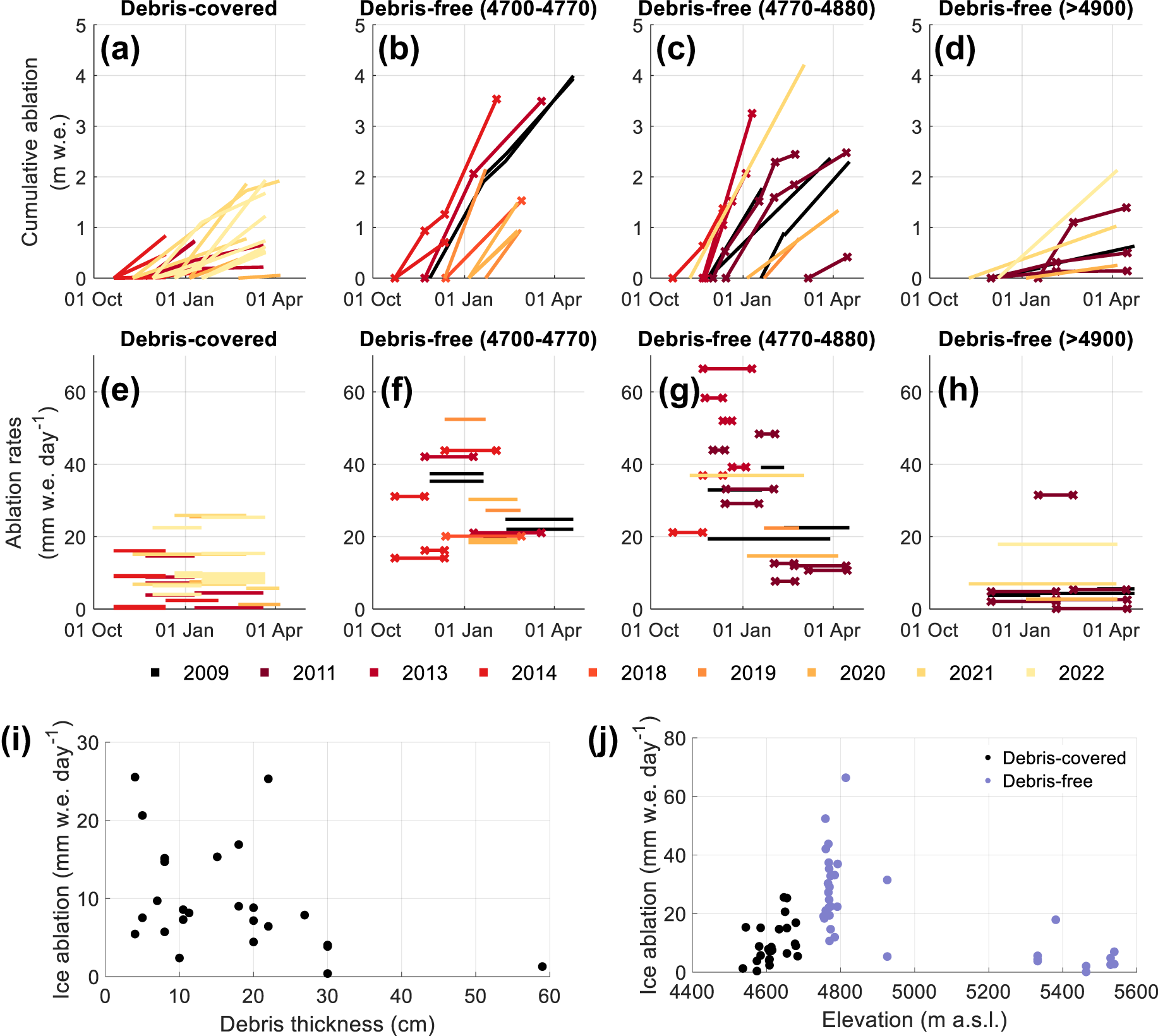
Figure 4. Summary of ablation measurements over different glacier sections since 2009 as a function of the ablation season (from October to May) showing the cumulative ablation (a–d) and ablation rates (e–f). The lines with the markers correspond to measurements at ablation frames. (i) Summer ablation rates at debris-covered sites as a function of debris thickness. (j) Summer ablation rates at debris-covered (red) and debris-free (blue) sites as a function of elevation.
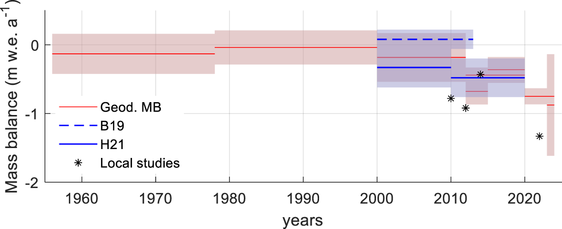
Figure 5. Geodetic mass balance of Tapado Glacier (debris-free and debris-covered sections) for the time periods presented in Table 4. The glacier-wide mass balance (Geod. MB) and its associated uncertainty are shown using red lines and shaded areas, respectively. B19 and H21 correspond to the results for Tapado Glacier in the studies by Braun and others (Reference Braun2019) and Hugonnet and others (Reference Hugonnet2021). The results from local studies using glaciological measurements are presented in black asterisks (Table S2). The results from local studies, B19 and H21 refer only to the debris-free section.
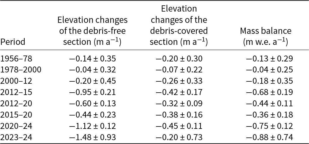
Table 4. Elevation changes and geodetic mass balance of Tapado Glacier
In addition to these point-scale results, we reviewed results for glacier-wide mass balances calculated in other studies, which correspond mostly to reports commissioned by Chilean Governmental agencies (Table S2). These studies made use of the same measurements presented here, but their results were derived using different methods and assumptions, so it is difficult to compare them directly. However, these do provide an approximate range of glacier mass balance variability. Results are reported for summer, winter and annual periods. Summer mass balance varied from −0.8 to −1.7 m w.e. season−1 on the debris-free section and from −0.5 to −0.6 m w.e. season−1 on the debris-covered section. Reported winter mass balance varied from 0.2 to 0.5 m w.e. season−1. In the next section, the available annual values from previous studies are normalised and compared against our geodetic mass balances.
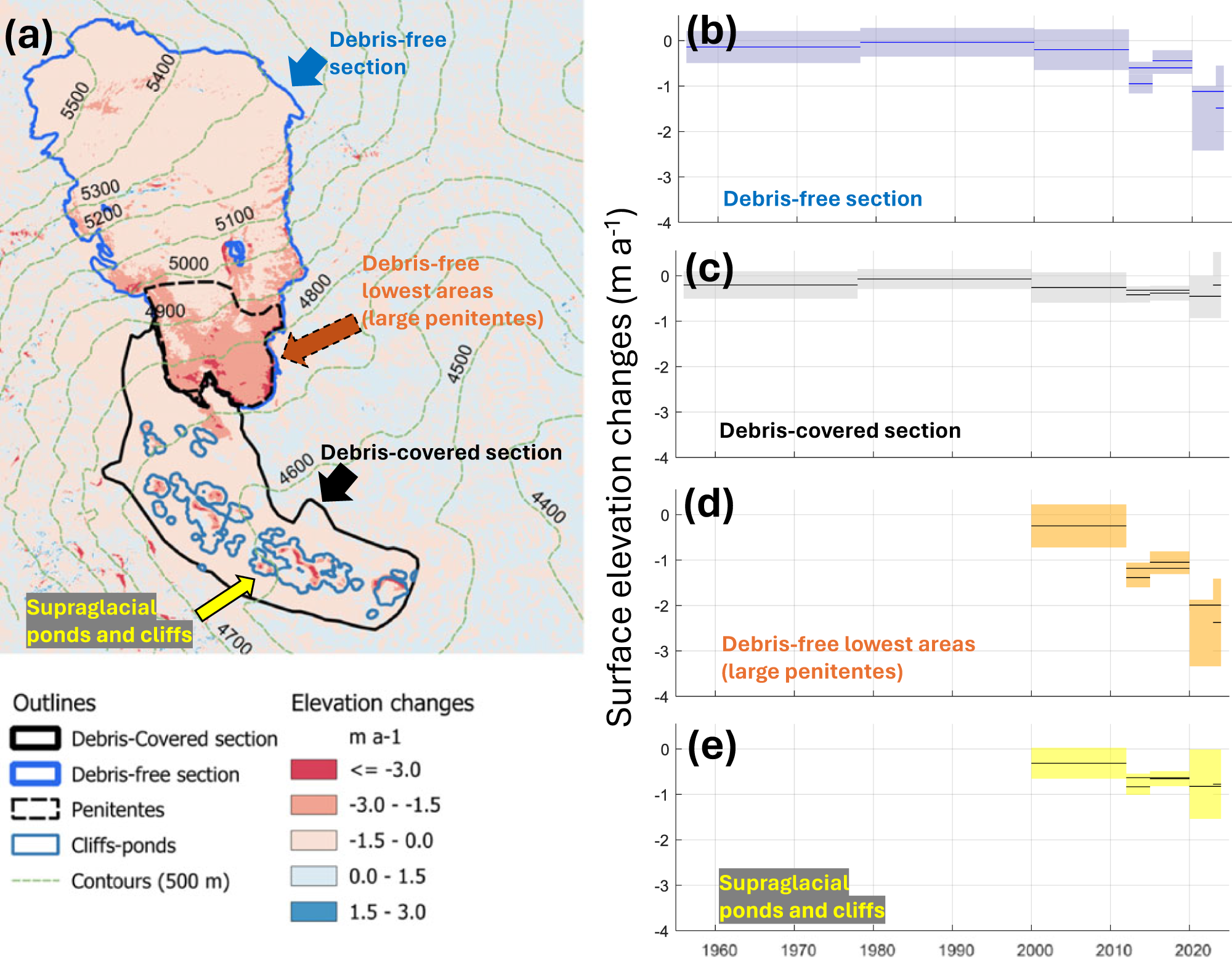
Figure 6. (a) Map of surface elevation changes in 2020–24. The polygons represent the glacier outlines (debris-free and debris-covered sections) and the area of penitentes and supraglacial ponds and cliffs. Surface elevation changes of the glacier sections shown in (a) since 1956: (b) debris-free section, (c) debris-covered section, (d) debris-free lowest areas and (e) supraglacial ponds and cliffs. The data for the periods before 2020 are extracted from Robson and others (Reference Robson, MacDonell, Ayala, Bolch, Nielsen and Vivero2022).
4.2.2. Geodetic mass balances and surface elevation changes
Figure 5 and Table 4 present the geodetic mass balance of Tapado Glacier (debris-free and debris-covered sections) since 1956 and the associated uncertainties. Figure 5 also shows a comparison with local studies and results extracted from the geodetic mass balance by Braun and others (Reference Braun2019) and Hugonnet and others (Reference Hugonnet2021) (Table S2). The results from these studies are for the debris-free section only. Our results indicate that the mass balance of Tapado Glacier varied from slightly negative in 1956–78 (−0.13 ± 0.29 m w.e. a−1) to almost balanced in 1978–2000 (−0.04 ± 0.25 m w.e. a−1). After the year 2000, the mass balance became increasingly more negative, varying from − 0.18± 0.35 m w.e. a−1 in 2000–12, to − 0.44± 0.11 m w.e. a−1 in 2012–20 and − 0.75± 0.12 m w.e. a−1 in 2020–24. Results from Braun and others (Reference Braun2019) suggest a slightly positive mass balance for the debris-free section between 2000 and 2013 (+0.08 m w.e. a−1), but these results might be affected by radar signal penetration (Dussaillant and others, Reference Dussaillant2019). The more negative mass balance of Tapado Glacier in the decade 2010–20 compared to 2000–10 can also be observed in the results from Hugonnet and others (Reference Hugonnet2021). Although there are only four comparable local studies, they also seem to confirm the main temporal patterns found by the geodetic mass balances.
To better visualise the distribution of geodetic change over the Tapado Glacier, we plot the spatially distributed average annual rates of surface elevation change derived from Pléiades and Pléiades Neo imagery for the period 2020–24 in Figure 6a. Surface lowering is observed over almost the entire glacier with values between −1.5 and −3.0 m a−1 over the lower areas of the debris-free section and between 0 and −1.5 m a−1 over the debris-covered section (except for ice cliffs and ponds) and the upper debris-free areas. These spatial patterns are similar to those observed in the glaciological observations (Fig. 4). The lower areas of the debris-free sections correspond to the location of the ice penitentes, whereas the largest lowering values observed over the debris-covered glacier appear to be associated with supraglacial ice cliffs and ponds (Fig. 6a).
To better understand the temporal and spatial patterns of thinning over the different glacier sections, Figure 6b–e show elevation changes for different glacier sections. These sections correspond to the debris-free and debris-covered sections, as well as to the ice penitentes and the area covering the evolution of the supraglacial ice cliffs and ponds over the debris-covered section. Although both the debris-free and debris-covered sections show increasing thinning after the year 2000 (Table 4 and Fig. 6b, c), in recent years the debris-free section presents larger values of thinning (−1.12 ± 0.12 m a−1 in the period 2020–24) than the debris-covered section (−0.45 ± 0.11 m a−1). In the debris-free section, the observed changes are driven by the penitentes area, which shows a strongly negative elevation change, until reaching a value of −1.99 ± 0.12 m a−1 in the period 2020–24. In the debris-covered section, the elevation change of the area containing ice cliffs and ponds has reached a value of −0.82 ± 0.11 m a−1 after 2020. Previous measurements have shown that the emergence velocities in the ablation areas of Tapado Glacier average 0.4 ± 1.1 m per ablation season (4–6 months) (CEAZA, 2012, 2021). These results suggest that surface mass losses at the lower areas of the debris-free section might have been compensated by the ice advection from the upper areas before the megadrought, but that average rates of ablation now exceed ice emergence.
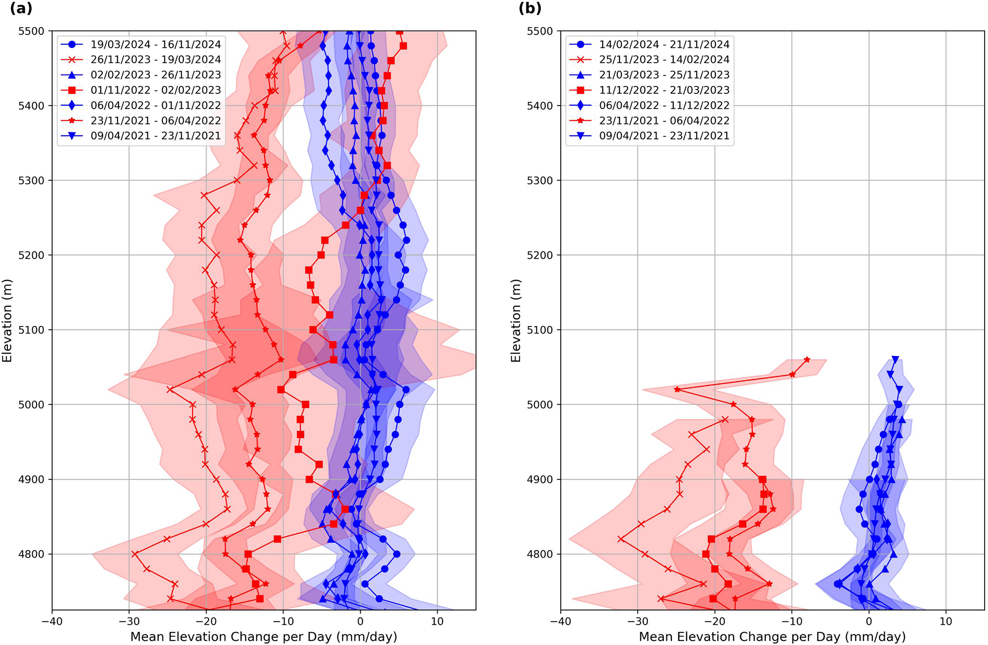
Figure 7. Seasonal profiles of surface elevation change over the debris-free section. (a) shows elevation profiles for the satellite products, while (b) shows the UAV-based elevation profiles. The LiDAR data are included in both plots. The shading for each elevation band represents one standard deviation of elevation change.
Seasonal elevation changes of the debris-free section, derived from the combination of LiDAR, Pléiades and the UAV surveys, show that winter balances have been characterised by almost no net accumulation since 2021 (Fig. 7). Figure 7a presents elevation profiles derived from Pléiades products that covered the entire elevation range of the debris-free section, whereas Figure 7b presents UAV-derived elevation profiles that covered up to ∼5050 m a.s.l. Results from the LiDAR surveys were included in both figures in order to extend the seasonal time series back to 2021. Although UAV-derived profiles do not cover the entire elevation range of the glacier, they allow for more precise estimates. Results show that summer thinning has been negative over the entire analysed elevation range (4700–5500 m a.s.l.) except for summer 2022–23. In general, elevation changes tend to be less negative towards higher elevations, ranging from −10 to −30 mm d−1 at the lower elevations and between −15 and +5 mm d−1. The negative elevation changes in the lower parts of the debris-free section highlight that ice emergence is not able to compensate for the summer melt. Winter elevation profiles do not show a clear relation with elevation and are around zero for all the analysed seasons.
4.3. Areal and morphological changes
4.3.1. Areal changes
We estimate that the debris-free section of Tapado Glacier has lost 35% of its area since 1956 (equivalent to 0.47 km2, Fig. 8 and Table S3). We identify two periods with different rates of area loss. On average the debris-free area was reduced at a rate of 0.004 km2 a−1 (−0.4% a−1) in the period 1956–2000 and 0.017 km2 a−1 (−1.7% a−1) since 2010. The changes are dominated mostly by the retreat of the debris-free lowest areas, but the glacier has also lost a significant part of its upper western section. On these slopes, the ice surface visible in the pre-2010 images may now be covered by debris falling from the upper, steep mountain ridges. The northern part of the glacier appears to have lost a large area, but these changes are difficult to distinguish as they are dominated by snow patches that can last for several years. The glacier outline was particularly challenging to delineate in the image from the year 2000, as it was taken in January and some snow may still remain from the extremely wet winter of 1997. Figure 8 also indicates that the debris-covered section has increased its size from 0.39 km2 in 1956 to 0.53 km2 in 2024 (equivalent to an increase of 36%). Thus, more than one-third of the area lost by the debris-free section since 1956 has been compensated by an increase in the debris-covered areas.
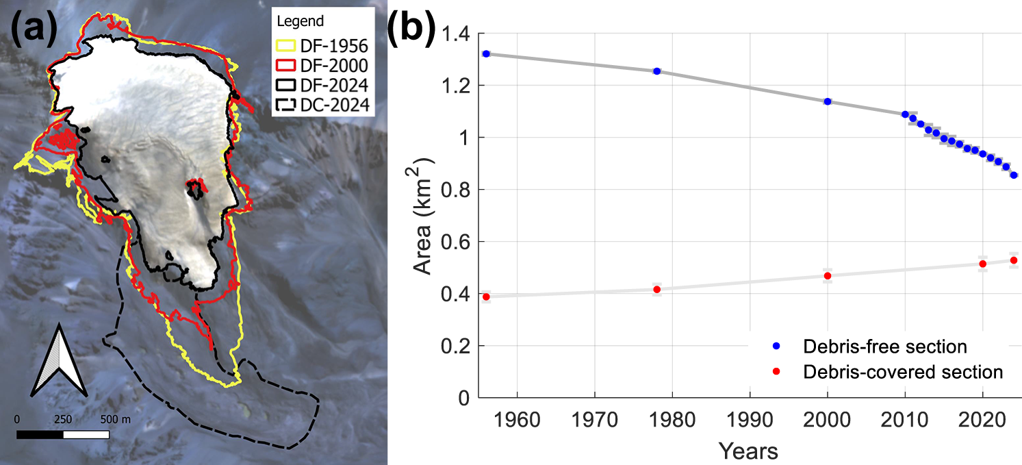
Figure 8. (a) Map with delineated outlines of debris-free Tapado Glacier for the images in 1956, 2000 and 2024 and debris-covered section in 2024, (b) Area changes of the debris-free and debris-covered sections since 1956. The background image in (a) corresponds to a Planet 2024 false colour composite.
4.3.2. Morphological changes
In this section, we present the results of the measurements of penitentes height at the end of the summer season using both manual observations (in the period 2011–22) and the UAV surveys (in the period 2019–24). Although the areas in which these observations were carried out do not overlap completely, they all correspond to the area where the largest ice penitentes develop (between 4700 and 4900 m a.s.l.). The manual measurements show a temporal evolution of penitentes height with two different phases (Fig. 9a). While from 2011–12 to 2014–15, penitentes height showed relatively stable values, with average values varying between 1.7 and 2.0 m, in 2018–19 to 2021–23, the penitentes height showed a steady increase from ∼0.8 m in 2018–19 to 3.0 m in 2021–22 and 2022–23. The elevation of the manual measurements range between 4750 and 4800 m a.s.l. The number of measurements per season varied between one and five.
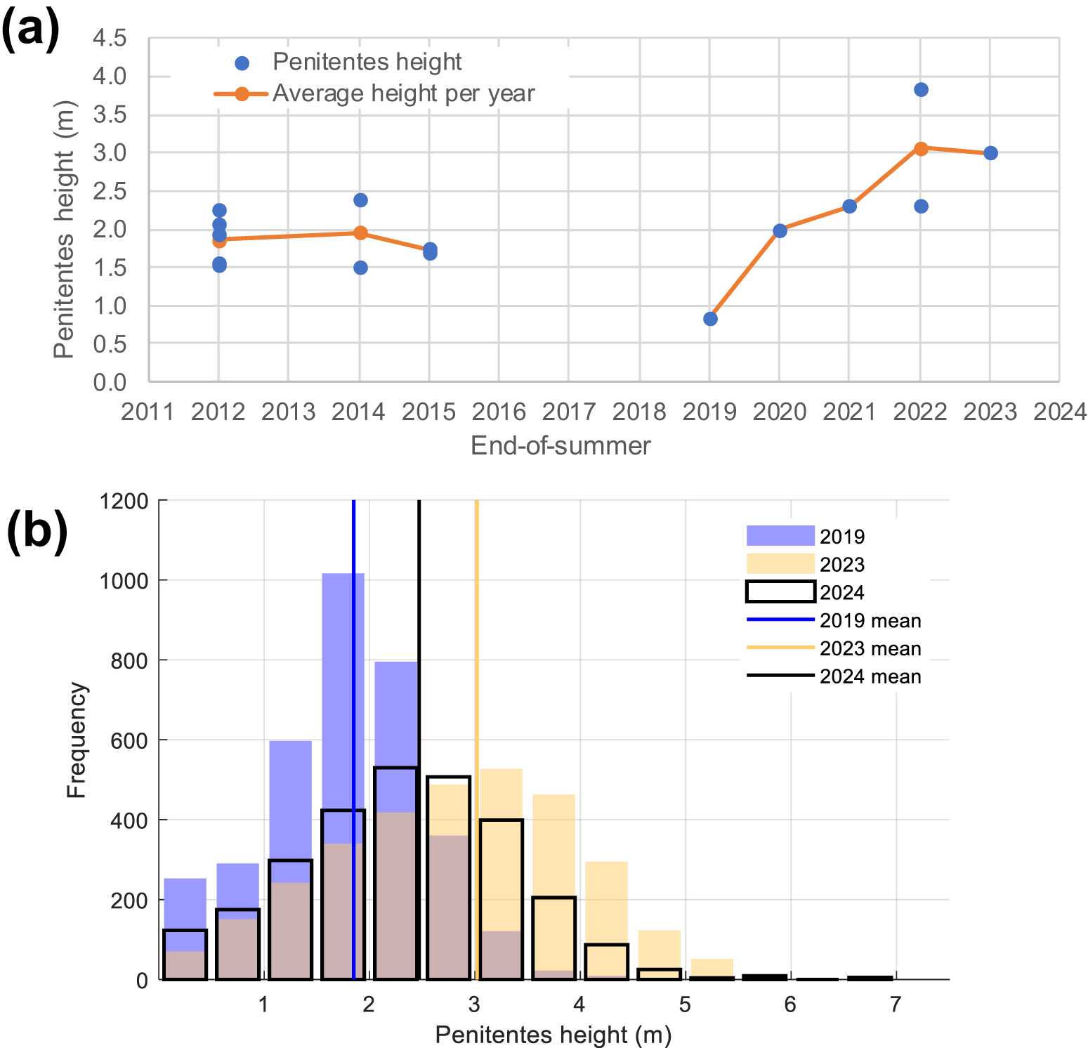
Figure 9. (a) Manual measurements of end-of-season penitentes height. Blue points represent individual measurements and orange points represent the average at each particular year. (b) Histograms of the height of the penitentes in 2019, 2023 and 2024, using the same area covered by the UAV survey in 2019 (see Figure 1c). Vertical lines show the mean of each distribution.
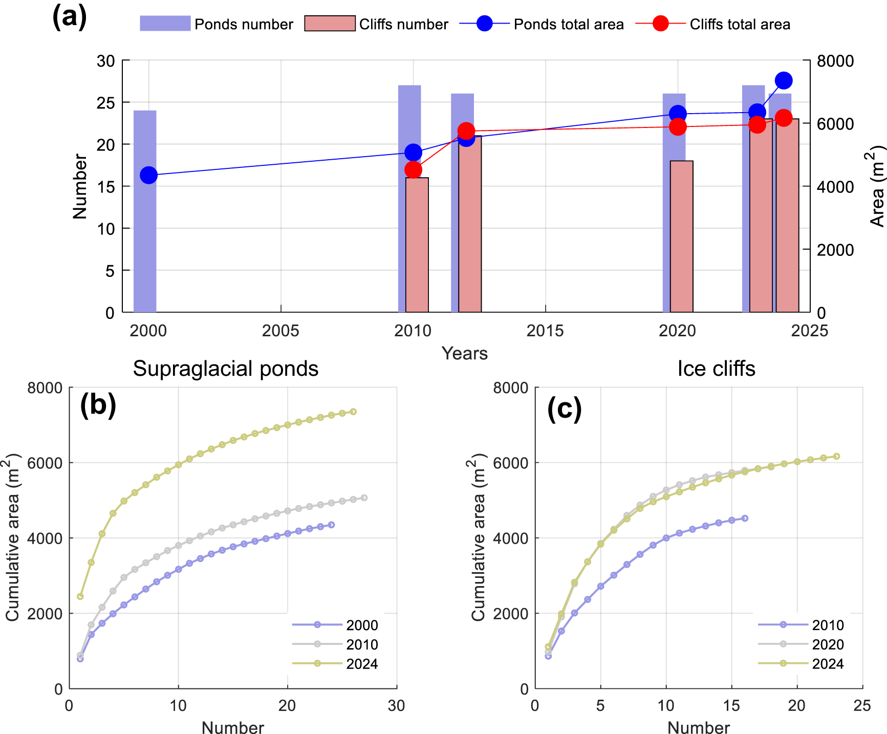
Figure 10. (a) Changes in the number and surface area of supraglacial ponds and ice cliffs larger than 40 m2 on Tapado debris-covered glacier. Cumulative distribution of the area of (b) supraglacial ponds and (c) ice cliffs as a function of their number.
Figure 9b shows the frequency distribution of the height of the penitentes obtained from the post-processing of the point clouds derived from the UAV surveys (Section 3.2.4). Conveniently, the first two surveys took place at the beginning and end of the penitente growth period (2019–23) identified in Figure 9a. We obtain an average penitente height of 1.85 and 3.02 m in 2019 and 2023, respectively. The average penitente height in 2024 was lower (2.47 m) than in 2023. In both 2023 and 2024, penitente heights of more than 5 m were identified, associated with the steep lateral edge of the debris-free glacier.
4.3.3. Supraglacial ponds and ice cliffs
Figure 10 shows the results of the temporal trends of supraglacial ponds and ice cliffs on the Tapado debris-covered glacier. The results of the manual delineation of supraglacial ponds show that the number of ponds on Tapado Glacier has remained relatively constant since 2000, but the total surface area of the ponds has increased by 45% (from ∼4450 to 7880 m2; Fig. 10a). This value is largely explained by the growth of the 10 largest ponds, whose total area doubled (from ∼3000 to 6000 m2) in the period 2000–24 (Fig. 10b). Changes in the number and area of ice cliffs are less clear. We found an increase in total area of 43% (from 4650 to 6660 m2, Fig. 10a), but with a relatively stable number in the period 2012–24. Most of the changes in total area occurred between 2010 and 2012. In contrast to the changes in the supraglacial ponds, the increase in total area of cliffs does not relate to the increase of the largest cliffs (Fig. 10c). However, it should be noticed that the total surface area of each cliff is larger than the measured one, as the latter corresponds to a horizontal projection.
4.3.4. Monitoring of the marginal ice surrounding the exposed bedrock (debris-free section)
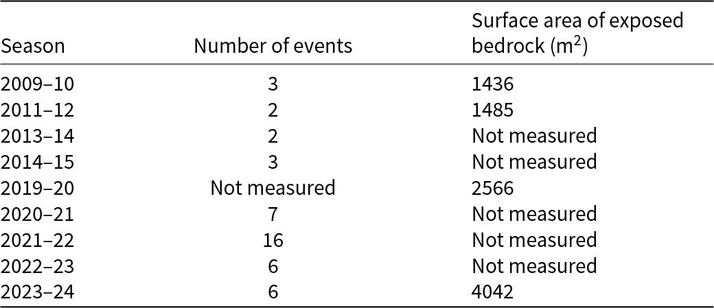
Table 5 shows the results of the visual analysis of the Tapado Glacier photos taken by the automatic cameras (described in Section 3.2.2). The pictures show a series of snow avalanches and serac fall events from the marginal ice surrounding the exposed bedrock in the debris-free section causing rock mobilisation that contribute debris to the lower tongue. In general, the number of these events was lower in the ablation seasons before 2015 (between two and three events per summer) than in the 2020–24 seasons (between six and seven events per summer). The number of events was particularly high during the 2021–22 season, with 16 events being observed. This number decreased to six events per summer in the following seasons. An example of an ice detachment from the ice cliff captured by the automatic camera and a satellite image is shown in Figure S4. The increase in the activity of the marginal ice has been accompanied by an increase in the area of the exposed bedrock. As shown in Table 5, our delineation of the exposed bedrock shows that since 2010 its surface has increased from ∼1400 to 4000 m2 (180% increase). Although there are some signs of its appearance before 2000, the feature cannot be clearly appreciated in the oldest available images.
Table 5. Number of snowfall and icefall events from the marginal ice surrounding the exposed bedrock in the debris-free section during the period December–April
4.3.5. Albedo changes
Albedo from Landsat surface reflectance indicates that the glacier surface has been darkening since ∼2005 (Fig. 11). Excluding the years with some snow cover, the summer minimum albedo was ∼0.4 until 2005. After that, the albedo has decreased to values below 0.2. The occasional summer snow cover is particularly noticeable in the summer after the extremely wet winter of 1997, which is related to the intense 1997–98 El Niño Southern Oscillation (ENSO) event. The year 2012 also appears as an anomaly in the general trend. Only one image was available that year during the time period used for the analysis (February-May). The image date is 2012-05-03 (doy = 124: note the black colour in the colourbar of Fig. 11), so it is affected by the snow deposited by a few snowfall events in April and May (detected also by the LAG_DGA meteorological station).
5. Discussion
5.1. Tapado glacier changes and drivers
Precipitation records from LAG_DGA show a large inter-annual and inter-decadal variability that is consistent with previous studies in the Chilean Central Andes (Masiokas and others, Reference Masiokas2012; González-Reyes and others Reference González-Reyes2017; Garreaud and others, Reference Garreaud, Boisier, Rondanelli, Montecinos, Sepúlveda and Veloso-Aguila2020). These studies have found that the temporal variability is strongly linked to ENSO and other ocean-atmosphere processes of lower frequency, such as the Pacific Decadal Oscillation (PDO) and the Southern Annular Mode (SAM). The precipitation deficits of the Chilean Megadrought (2010 to present) in north-central Chile have been characterised by the southward migration of the South Pacific Subtropical High (Kinnard and others, Reference Kinnard2020) and have been explained by the combination of both natural variability and anthropogenic forcing (Garreaud and others, Reference Garreaud, Boisier, Rondanelli, Montecinos, Sepúlveda and Veloso-Aguila2020). In the LAG_DGA record, the period of the Chilean Megadrought presents a precipitation deficit of 43% compared to the period 1965–2009 (Fig. 3a) and can be roughly divided into two dry periods, one from 2009 to 2014 and a second from 2018 to 2023. However, the exact length of each period depends on the chosen location due to the spatial variability of precipitation in the Elqui River basin. Although the Chilean Megadrought in north-central Chile was interrupted by a period of relatively humid conditions between 2015 and 2017, the downstream areas of Tapado Glacier have been almost constantly under water stress since the beginning of the drought, most likely influenced by hydrological memory and water extractions (Valois and others, Reference Valois, MacDonell, Núñez Cobo and Maureira-Cortés2020; Álamos and others, Reference Álamos, Alvarez-Garretón, Muñoz and González-Reyes2024). We also identified a significant increase in annual air temperature since the 1970’s with an average increase of 0.29°C decade−1. These results are consistent with a generalised air temperature increase that has been observed along the Andes (Burger and others, Reference Burger, Brock and Montecinos2018; Masiokas and others, Reference Masiokas2020; Pabón-Caicedo and others, Reference Pabón-Caicedo2020). Although there are no long-term records of humidity in the Dry Andes, climate reanalysis data show a decrease in humidity since the 1980s (Robson and others, Reference Robson, MacDonell, Ayala, Bolch, Nielsen and Vivero2022).
The mass balance of the Tapado Glacier has become increasingly more negative in recent decades, varying from slightly negative values before 2000 to −0.18 ± 0.35 m w.e. a−1 in 2000–12, −0.44 ± 0.11 m w.e. a−1 in 2012–20 and −0.75 ± 0.12 m w.e. a−1 after 2020. The geodetic mass balance in the period 2020–24 is more negative than in the previous periods and similar to the values estimated for 2012–15, which corresponds to the first dry period of the Chilean Megadrought (Robson and others, Reference Robson, MacDonell, Ayala, Bolch, Nielsen and Vivero2022). We are confident in our glacier mass balance estimates as these are in line with the results from local glaciological studies (CEAZA, 2015, 2021, 2022) and those from Hugonnet and others (Reference Hugonnet2021). Surface lowering maps also suggest that mass loss is mostly driven by the ablation of penitentes covering the lowest debris-free areas and ice cliffs and ponds on the debris-covered section (Fig. 6), which are discussed in Section 5.2. The more negative mass balance obtained for Tapado Glacier in recent decades, especially after 2010, is similar to those obtained for other individual glaciers in the Dry Andes, such as Echaurren Glacier (Masiokas and others, Reference Masiokas2016; Farías-Barahona and others, Reference Farías-Barahona2019), Guanaco Glacier (Kinnard and others, Reference Kinnard2020) and Agua Negra Glacier (Pitte and others, Reference Pitte2022). This trend has also been observed in regional studies (Dussaillant and others, Reference Dussaillant2019; Caro and others, Reference Caro, Condom, Rabatel, Champollion, García and Saavedra2024).
The recent decrease in winter precipitation has resulted in little snow accumulation over the glacier (Fig. 7) and an early exposure of the ice surface, producing a decreasing trend of the annual minimum albedo, typically observed by the end of the ablation season (Fig. 11). The detected decrease in surface albedo has been also observed in other glaciers of the Southern Andes (Shaw and others, Reference Shaw, Ulloa, Farías-Barahona, Fernandez, Lattus and McPhee2021; Podgórski and others, Reference Podgórski, Pętlicki, Fernández, Urrutia and Kinnard2023). Along with the darkening of the glacier surface due to local dust and contamination (Sinclair and MacDonell and others, Reference Sinclair and MacDonell2016; Cordero and others, Reference Cordero2019; Barraza and others, Reference Barraza, Lambert, MacDonell, Sinclair, Fernandoy and Jorquera2021), the debris-free section of Tapado Glacier has considerably shrunk (Fig. 8). We estimate that the area of the debris-free section has reduced by 35% since 1956, which is mostly explained by the retreat of its lowest areas. This reduction has been partly compensated by an upward increase in the debris-covered section. We found that the rate of area loss has increased by more than four times after 2010 compared to the period 1956–2010. In contrast, the decrease in surface albedo started around 2000, before the onset of the Chilean Megadrought (Fig. 11).
According to several authors (e.g. Masiokas and others, Reference Masiokas2016; Kinnard and others, Reference Kinnard2020), glacier mass balance in the Dry Andes is mostly linked to precipitation and humidity variations, with air temperature playing a more relevant role towards the Wet Andes (south of 36° S). We suggest that the accelerated recent changes in mass balance, surface albedo and glacier area have been caused by the combination of the drought and the sustained temperature increase since the 1970s. Although similar dry periods have been observed in the past, they did not occur with such high temperatures, likely explaining the lower retreating rates observed in the past. In addition to the changes in precipitation and air temperature, as shown by Kinnard and others (Reference Kinnard2020) for Guanaco Glacier (to the north of Tapado Glacier), the decrease in humidity might have also played a role in the negative mass balances by increasing sublimation, particularly in the upper glacier areas. However, it is not fully clear exactly how the drying and warming trends, likely causing sublimation and melt to increase, have combined to drive the Tapado Glacier retreat and negative mass balances. In Section 5.2, we discuss how the new datasets presented in this article could shed some new light on the specific processes driving mass loss and the future evolution of Tapado Glacier.
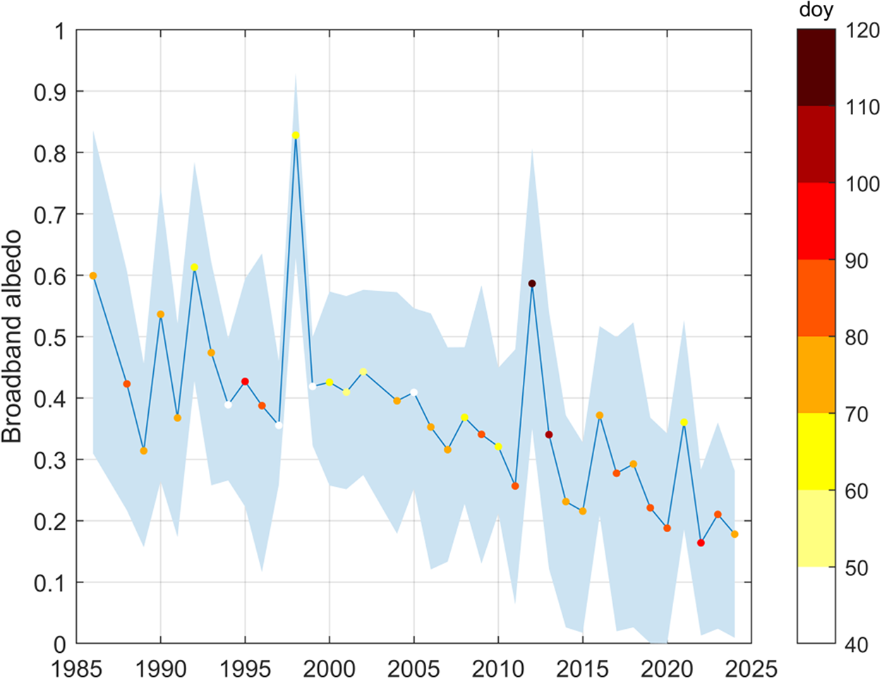
Figure 11. Annual minimum broadband albedo of the debris-free section as obtained from the surface reflectance of the Landsat archive (Knap and others, Reference Knap, Reijmer and Oerlemans1999). The line shows the glacier-wide average and the envelope indicates the 10th and 90th percentile of the spatial variability. Colourbar indicates the mean day of year (doy) of the minimum albedo retrieved at each pixel.
5.2. Processes driving mass loss and future evolution
The results derived from manual measurements and UAV flights, as well as field observations, indicate that the average size of penitentes increased by more than 1 m in the period 2019–23 (Fig. 9 and S1), particularly at the margins of the debris-free section, where they have reached heights of more than 10 m (Fig. 9 and Fig. S1). Manual records before 2015 show that penitentes have reached heights of more than 2 m in the past (Fig. 9a). This suggests that the space between the penitentes was filled by snow accumulation in the more humid winters between 2015 and 2017, which could explain the relatively small size of the penitentes in 2019. An alternative explanation could be an increased ablation at the top of the penitentes caused by, for example, switching from sublimation to melt as the dominant process in the humid winters between 2015 and 2017. Such a process would cause a smaller difference between the ablation rates at the top and at the troughs of the penitentes. That explanation is similar to that proposed to explain the decay of ice sails in the central Karakoram mountain region (Evatt and others, Reference Evatt, Mayer, Mallinson, Abrahams, Heil and Nicholson2017). After the humid winters of 2015–17, the series of dry winters between 2018 and 2022 resulted in little snow accumulation and an extended ablation period to carve penitentes during summer. Furthermore, increasing summer air temperatures have resulted in high rates of surface lowering (Fig. 6b and d). The relatively flat area selected as representative of ice penitentes covers only 16% of the debris-free section (see Fig. 6a), but we estimate that its net mass loss in the period 2020–24 is equivalent to 34.5 ± 2.0% of the section net losses. This estimate was obtained by converting the average elevation changes to surface mass balance using a range of emergence velocities measured over the ice penitentes during previous studies (0.4 ± 1.1 m season−1). Interestingly, results derived from the 2024 UAV flight show that the height of the penitentes decreased compared to that of 2023. Indeed, some of the images captured during the UAV flights show the presence of large debris-filled sections between the penitentes close to the edge of the debris-free ice (Fig. S5). Although this debris may have been brought by meltwater from upper areas, it can be hypothesised that it corresponds to the surface of an upper debris-covered section below the ice surface over which the penitentes have developed until now. Indeed, field observations suggest that this ice surface is constituted by a significant proportion of superimposed ice. If this is the case, penitentes will likely become smaller in size, the ablation rates over this section will decrease and a new debris-covered surface will be exposed.
Ice cliffs and supraglacial ponds drive glacier ablation on debris-covered glaciers, where the ice melt rates are typically low due to the thermal insulation and protection against solar radiation provided by the debris (Miles and others, Reference Miles, Hubbard, Irvine-Fynn, Miles, Quincey and Rowan2020). Indeed, ice cliffs can be considered as hotspots for melt (Barraza and others, Reference Barraza, Lambert, MacDonell, Sinclair, Fernandoy and Jorquera2021; Ferguson and Vieli, Reference Ferguson and Vieli2021). For example, Buri and others (Reference Buri, Miles, Steiner, Ragettli and Pellicciotti2021) found that ice cliffs occupy ∼2% of the surface area of the debris-covered glacier tongues in the Langtang catchment (Nepal) but can represent ∼17% of their ice mass loss. Similarly, we estimate that the net mass loss of the area comprising the location of cliffs and ponds on Tapado Glacier (see Fig. 6a) is equivalent to 82.1 ± 0.4% of the net loss of the debris-covered glacier in the period 2020–24, despite representing only 45% of its area. Ice cliffs can be clearly observed in the map of elevation changes (Fig. 6a) and their total area has increased since 2010, as well as the total area of supraglacial ponds (Fig. 10). However, in contrast to the accelerating ablation rates of penitentes, the ablation rates of the debris-covered section have increased more slowly (Fig. 6c). This stabilisation may be connected to thicker debris produced by its mobilisation (Westoby and others, Reference Westoby2020). The increase in the total area covered by supraglacial ponds could indicate a longer retention time of meltwater within the debris-covered glacier, modifying the role it plays in glacier discharge to the catchment (Pourrier and others, Reference Pourrier, Jourde, Kinnard, Gascoin and Monnier2014). For example, it is possible that a larger proportion of meltwater is evaporating rather than being discharged. Similar increases in the total area of supraglacial ponds have been found in other mountain areas, such as the Everest region (Watson and others, Reference Watson, Quincey, Carrivick and Smith2016).
A different type of change in the driving processes of glacier ablation might be occurring on the upper areas of Tapado Glacier. In those areas, sublimation largely dominates over melt (Ginot and others, Reference Ginot, Kull, Schwikowski, Schotterer and Gäggeler2001), but the decrease in surface albedo and the increase in summer air temperature might be triggering a shift from sublimation to more melt-dominated conditions. Similar processes have been proposed in the Peruvian Andes (Fyffe and others, Reference Fyffe2021). Such a shift would increase the amount of water in the upper areas and affect the structural stability of the glacier, particularly of the marginal ice surrounding the exposed bedrock in the debris-free section (Table 5). Under extremely warm conditions, the chances for destabilisation at the steep bedrock interface could increase as the glacier warms and more meltwater are available in the subglacial system (Bondesan and Francese, Reference Bondesan and Francese2023). The observation of high-resolution images does not indicate changes in the width of crevasses on the upper area, but more detailed analyses including ice dynamics are needed.
The recent changes in Tapado Glacier are characterised by accelerated losses of glacier area and mass. These losses have been driven by dry periods that resulted in minimal snow accumulation during winter, which thus caused a sustained lowering of glacier-wide surface albedo, and increasing air temperatures, which have caused increased ablation rates. However, this phase of accelerated changes is likely to be transient. We suggest that, as the ice volume available for melt reduces, the current transitional phase may end with the glacier eventually reaching more stable conditions. These conditions will likely be characterised by a disconnected debris-covered stagnant ice below a thick debris layer, on which no more ice cliffs or ponds develop, and an upper, high-elevation dome. As the ice thins, it is possible that new areas covered by debris may emerge at previously penitente-covered sections. The end of the Megadrought and the return to more humid conditions, such as those observed in the 1980s, may increase winter accumulation, but the increasing global temperatures are likely to maintain the negative mass balances.
Key limitations of our study are the absence of in situ winter mass balance and the lack of measurements on the ice penitentes during the last few years due to difficulties accessing that area. These issues prevent or make difficult the disaggregation of the surface mass balance into its seasonal components, which are directly connected to climatic variations. In order to simulate the future mass balance and evolution of Tapado Glacier, we recommend the application of modelling strategies that integrate individual parameterisations of the physical processes analysed in this study. Of particular importance are an energy balance model capable of solving sublimation and melt of snow and ice penitentes, a parameterisation of the ice flow and mass transfer from the debris-free section to the debris-covered one and a representation of the ablation at supraglacial ponds and cliffs on the debris-covered section. Ongoing field monitoring of Tapado Glacier mass balance and processes should continue focusing on long-term climate and mass balance variations, as well as on process understanding. An interesting possibility for the upcoming decades is the extraction of an ice core from the summit of Tapado Glacier (such as in the pioneering study from Ginot and others [Reference Ginot, Kull, Schotterer, Schwikowski and Gäggeler2006]) to evaluate the impact of the Chilean Megadrought on the dynamics of accumulation and ablation in the upper glacier areas. A periodic re-assessment of the connectivity between the debris-free and the debris-covered sections is also recommended.
6. Conclusions
Tapado Glacier is one of the largest glaciers in north-central Chile. It plays an important hydrological role for the Elqui River basin and is a key site for the monitoring of climate changes in the Dry Andes as it lies in a transition zone from the Atacama Desert to more Mediterranean-type climates to the south. Glacier mass loss is governed by various processes that control the evolution of different surface types and elements, such as ice penitentes, debris-covered ice, supraglacial ice cliffs and ponds and others. We use remote sensing products and a large dataset of meteorological and glaciological data collected on Tapado Glacier and its surroundings to describe its major changes and the physical processes driving glacier mass loss. We summarise our findings as follows:
- The period 1965–2024 was characterised by a sequence of dry periods with very low precipitation and a significant increase in annual mean air temperature of 0.29°C decade−1, resulting in an increase of 1.5°C in the last 50 years. Winter precipitation since the beginning of the Chilean Megadrought in 2010 has been 43% lower than the 1965–2009 average.
- The observed changes in meteorological variables have led to more negative glacier mass balance, a reduction of the debris-free area and a decrease in surface albedo. The mass balance of the Tapado glacier has become increasingly more negative in recent decades, varying from slightly negative values before 2000 to −0.18 ± 0.35 m w.e. a−1 in 2000–12, −0.44 ± 0.11 m w.e. a−1 in 2012–20 and −0.75 ± 0.12 m w.e. a−1 after 2020. The debris-free area decreased at a rate of 0.004 km2 a−1 (−0.4 % a−1) in the period 1956–2000 and 0.017 km2 a−1 (−1.7 % a−1) since 2010.
- The areas characterised by ice penitentes on the lower debris-free section and supraglacial ice cliffs and ponds over the debris-free section correspond to 26% of the glacier area, but their net mass losses are equivalent to ∼43% of the total net loss in the period 2020–24. Morphological changes on these sections have been particularly large since 2019, with ice penitentes increasing their average size by at least 1 m and supraglacial ponds increasing their area by 43%. The upper surface areas may be shifting from a sublimation- to a melt-dominated environment, adding meltwater to the subglacial system and increasing the fall of snow and ice from the marginal ice surrounding a steep area of exposed bedrock.
We hypothesise that the accelerated changes taking place on Tapado Glacier are likely to be transient and the glacier might reach a new state characterised by less dynamic conditions. In this new state, the glacier would retreat to an upper high-elevation ice dome on the summit of Cerro Tapado, whereas the debris-covered section would evolve into a disconnected mass of stagnant ice covered by thick debris. The diversity of processes controlling the changes and mass loss of the Tapado glacier requires the use of multiple techniques and tools. Detailed modelling of the past and future evolution of the glacier also requires the combination of modules that are usually separate, such as energy balance and debris mobilisation models. The Tapado Glacier clearly exemplifies the accelerated response of the Andean cryosphere to recent climate changes.
Supplementary material
The supplementary material for this article can be found at https://doi.org/10.1017/jog.2025.24.
Acknowledgements
The authors thank a series of projects financed by DGA between 2012 and 2024, the Coquimbo Regional Government (BIP 40000343) and ANID-Centro Regionales (R20F0008). ÁA acknowledges ANID-Fondecyt Postdoc 3190732. MP acknowledges ANID-Fondecyt Regular 1220978. The authors wish to thank the European Space Agency for the free provision of the SPOT, Pléiades and Pléiades Neo imagery through the restrained dataset projects RITM0114011, RITM0088590 and 41743. Over the years, the monitoring of Tapado Glacier has been made possible by the participation of several individuals, including former members of the CEAZA glaciology group, researchers, field assistants, students, local mountain guides, interns, local inhabitants and guests, all of whom are gratefully acknowledged. We thank the editor Dr Evan Miles and two anonymous reviewers for their thoughtful comments that helped to improve the manuscript. The ablation stakes measurements, 3D meshes of the penitentes in 2019 and 2023 and the geodetic mass balance and uncertainties in 2020–24 and 2023–24 are available at 10.5281/zenodo.14755911. A visualization of the 3D meshes of the penitentes is also available at https://skfb.ly/p76Nv and https://skfb.ly/p76Nv. The rest of the datasets are available upon request.


 Open access