


1. Introduction
The importance of the Arctic sea ice cover in the climate system stems primarily from its influence on the Earth’s radiation budget, which it exerts through its relatively large albedo (Kwok & Untersteiner Reference Kwok and Untersteiner2011). Despite its importance, predicting changes in the ice cover accurately, subject to prescribed forcings, still remains challenging. One of the principal challenges associated with making this prediction is related to the dynamics of the ice cover (Rothrock Reference Rothrock1975a ; Kwok & Untersteiner Reference Kwok and Untersteiner2011; Rampal et al. Reference Rampal, Weiss, Dubois and Campin2011; Fox-Kemper et al. Reference Fox-Kemper2021).
The ice cover is not continuous, but is made up of a very large number of floes of different shapes, sizes and thicknesses (Thorndike et al. Reference Thorndike, Rothrock, Maykut and Colony1975; Rothrock & Thorndike Reference Rothrock and Thorndike1984). It can be inferred from field and satellite observations that sea ice behaves differently at different length scales: at the scale of an individual floe it moves like a deformable solid body (Parmerter Reference Parmerter1975; Vella & Wettlaufer Reference Vella and Wettlaufer2008), but at much larger scales it moves like a highly viscous fluid (Reed & Campbell Reference Reed and Campbell1962). This suggests that the following two approaches can be used to study its motion (see Solomon (Reference Solomon1970) for a more general discussion).
-
(i) In the first approach, the motion of individual ice floes is studied by solving Newton’s equations for each floe taking into account any floe–floe interactions. From these solutions, one then extracts statistical information (Thorndike & Colony Reference Thorndike and Colony1982; Colony & Thorndike Reference Colony and Thorndike1984, Reference Colony and Thorndike1985; Thorndike Reference Thorndike1986; Rampal et al. Reference Rampal, Weiss, Marsan and Bourgoin2009; Agarwal & Wettlaufer Reference Agarwal and Wettlaufer2017) that is used to describe the motion of the ice cover at much larger length scales.
-
(ii) In the second, one takes the ice cover to be a continuum and develops rheological models to relate the internal stress field to the other macroscopic variables, including the thickness distribution of ice (Thorndike et al. Reference Thorndike, Rothrock, Maykut and Colony1975; Toppaladoddi & Wettlaufer Reference Toppaladoddi and Wettlaufer2015, Reference Toppaladoddi and Wettlaufer2017; Toppaladoddi, Moon & Wettlaufer Reference Toppaladoddi, Moon and Wettlaufer2023). This is then used in the Cauchy equation, with appropriate boundary conditions, to solve for the velocity field.
A principal aim of both these approaches is to predict the statistical properties of the ice velocity field. Both approaches have their advantages and limitations, but the focus since the Arctic Ice Dynamics Joint Experiment (AIDJEX) expedition in the 1970s has been on developing observationally consistent rheological models (Rothrock Reference Rothrock1975a ; Feltham Reference Feltham2008).
The first attempt to include floe–floe interactions into the dynamics of sea ice was by Sverdrup (Reference Sverdrup1928). He represented the internal ice resistance using a frictional force that was proportional to the floe velocity, but always in the direction opposite to it. However, this formulation is not completely correct as friction can both decelerate and accelerate an object depending on the relative velocity (Reed & Campbell Reference Reed and Campbell1962; Solomon Reference Solomon1970). A more generalised description of the floe–floe interactions was developed by Solomon (Reference Solomon1970) and Timokhov (Reference Timokhov1970), who considered deterministic and stochastic drift of ice, respectively, in one dimension. In a more general approach, the ice cover has been treated as a two-dimensional granular gas to understand the emergence of internal stress from floe–floe collisions (Shen, Hibler & Leppäranta Reference Shen, Hibler and Leppäranta1987) and the motion of ice floes in the marginal ice zone (Feltham Reference Feltham2005).
In order to study the emergence of internal stress from floe–floe collisions and the fracturing of floes, detailed numerical investigations have been performed using the molecular dynamics (Herman Reference Herman2011, Reference Herman2013) and discrete element modelling (Hopkins Reference Hopkins1996; Hopkins & Thorndike Reference Hopkins and Thorndike2006; Herman Reference Herman2016) approaches. Furthermore, new discrete element methods have been developed to: (i) simulate ice dynamics in a Lagrangian frame (Damsgaard, Adcroft & Sergienko Reference Damsgaard, Adcroft and Sergienko2018); (ii) resolve changes in the floe geometry resulting from collisions and mechanical deformation (Manucharyan & Montemuro Reference Manucharyan and Montemuro2022); (iii) capture dynamic sea ice patterns (West et al. Reference West, O’Connor, Parno, Krackow and Polashenski2022); (iv) study pressure ridging (Damsgaard, Sergienko & Adcroft Reference Damsgaard, Sergienko and Adcroft2021); and (v) understand the interactions between sea ice and ocean waves (Herman Reference Herman2017). These new methods use different models to represent floe–floe interactions, including Coulomb friction models (Damsgaard et al. Reference Damsgaard, Adcroft and Sergienko2018; Manucharyan & Montemuro Reference Manucharyan and Montemuro2022).
More recently, the $\mu (I)$
rheology – which was originally developed to model the viscoplastic flows of dense granular materials (da Cruz et al. Reference da Cruz, Emam, Prochnow, Roux and Chevoir2005) – has been used to describe the flow of sea ice in the marginal ice zone. Herman (Reference Herman2022) and de Diego et al. (Reference de Diego, Gupta, Gering, Haris and Stadler2024), assuming sea ice rheology to be the
$\mu (I)$
rheology – which was originally developed to model the viscoplastic flows of dense granular materials (da Cruz et al. Reference da Cruz, Emam, Prochnow, Roux and Chevoir2005) – has been used to describe the flow of sea ice in the marginal ice zone. Herman (Reference Herman2022) and de Diego et al. (Reference de Diego, Gupta, Gering, Haris and Stadler2024), assuming sea ice rheology to be the $\mu (I)$
rheology, have used data from their discrete element simulations to infer the friction coefficient,
$\mu (I)$
rheology, have used data from their discrete element simulations to infer the friction coefficient, $\mu$
, and dilatancy,
$\mu$
, and dilatancy, $\Phi$
, as functions of the inertial number,
$\Phi$
, as functions of the inertial number, $I$
, which is defined as the ratio of inertial to pressure forces (da Cruz et al. Reference da Cruz, Emam, Prochnow, Roux and Chevoir2005). The dimensionless parameter
$I$
, which is defined as the ratio of inertial to pressure forces (da Cruz et al. Reference da Cruz, Emam, Prochnow, Roux and Chevoir2005). The dimensionless parameter $I$
determines the state of the system which can be quasistatic (
$I$
determines the state of the system which can be quasistatic ( $I \leqslant 10^{-3}$
) or collision dominated (
$I \leqslant 10^{-3}$
) or collision dominated ( $I \geqslant 10^{-1}$
), with an intermediate transition regime (
$I \geqslant 10^{-1}$
), with an intermediate transition regime ( $10^{-3} \lt I \lt 10^{-1}$
) (da Cruz et al. Reference da Cruz, Emam, Prochnow, Roux and Chevoir2005).
$10^{-3} \lt I \lt 10^{-1}$
) (da Cruz et al. Reference da Cruz, Emam, Prochnow, Roux and Chevoir2005).
Simulating the dynamics of individual floes using discrete element methods provides the most detailed description of the ice cover; however, this approach becomes computationally prohibitive when extended to large spatial domains (Manucharyan & Montemuro Reference Manucharyan and Montemuro2022). One way to circumvent this computational difficulty is through the use of a continuum description of the ice cover. The collective motion of ice floes on length scales much larger than the floe scale can be approximated as that of a continuum (Thorndike et al. Reference Thorndike, Rothrock, Maykut and Colony1975). In this case, the equations that describe the evolution of the ice cover are the mass balance and Cauchy equations (Untersteiner Reference Untersteiner1986). The principal challenge associated with this approach has been in determining the constitutive equation for the internal stress (Rothrock Reference Rothrock1975a ). This task is made more difficult by the fact that the stress field in the ice cover depends not just on strain and strain rate but also on ice thickness and its distribution (Untersteiner Reference Untersteiner1986). Hence, understanding the coupling between the dynamics and the state of the ice cover, which is quantified by the thickness distribution of sea ice (Thorndike et al. Reference Thorndike, Rothrock, Maykut and Colony1975; Toppaladoddi & Wettlaufer Reference Toppaladoddi and Wettlaufer2015), is necessary.
The internal stress field in the ice cover is a consequence of the mechanical interactions between the constituent ice floes (Evans Reference Evans1970; Rothrock Reference Rothrock1975a ). However, unlike in the kinetic theory of gases, where molecules are assumed to interact only via elastic collisions (Harris Reference Harris1971; Chapman & Cowling Reference Chapman and Cowling1990), there are different modes of interaction – rafting, ridging, shearing and jostling – between ice floes (Parmerter & Coon Reference Parmerter and Coon1972; Rothrock Reference Rothrock1975a ; Parmerter Reference Parmerter1975; Vella & Wettlaufer Reference Vella and Wettlaufer2008). This makes it more challenging to develop a Boltzmann-like theory for the velocity distribution, although the development of such a theory has been attempted in the context of Saturn’s rings (Goldreich & Tremaine Reference Goldreich and Tremaine1978), where the shearing and jostling modes of interaction between ice particles are possible. In addition to the above four modes, the individual ice floes can also fracture due to thermal stresses (Evans & Untersteiner Reference Evans and Untersteiner1971) and due to interactions with ocean waves (Asplin et al. Reference Asplin, Galley, Barber and Prinsenberg2012).
A feature that is common to all these modes of interaction is that they happen over time and length scales much shorter than those that characterise the geophysical-scale evolution of the ice cover (Toppaladoddi & Wettlaufer Reference Toppaladoddi and Wettlaufer2015). This naturally leads to the following questions which any theory of sea ice rheology must address in one form or another. (i) What contributions do these different modes of interaction make to the rheology of the ice cover? (ii) What modes of interaction are important on different time scales? (iii) How are these interactions incorporated into a continuum description of the ice cover? Indeed, we will use these questions to guide us in the development of our own theory. In the development of viscous and plastic rheological models for sea ice, considerable emphasis was placed on the connection between the floe–floe interactions and the continuum behaviour (Rothrock Reference Rothrock1975a ). For this reason, we present a detailed discussion of these models here.
Some of the earliest rheological models proposed to study ice dynamics were the viscous models (Reed & Campbell Reference Reed and Campbell1962; Campbell Reference Campbell1965; Rothrock Reference Rothrock1975a ). Based on their qualitative observations of sea ice motion, Reed & Campbell (Reference Reed and Campbell1962) argued that the floe–floe interactions (shearing and jostling) should transport momentum from the faster moving to slower moving regions of the ice cover. This led them to propose a Newtonian rheology for sea ice. Subsequently, Nye (Reference Nye1973) and Hibler (Reference Hibler1977) provided more detailed arguments for the viscous behaviour to be viewed as the averaged response of the ice cover over long time and large length scales. There are a few variants of the viscous model that have been suggested, but not all are physically consistent (Rothrock Reference Rothrock1975a ).
The viscous model of Rothrock (Reference Rothrock1975a ,Reference Rothrock b ), in combination with a divergence-free velocity field, produces realistic drift of the Arctic ice cover. However, the viscous models of sea ice, in general, suffer from the following two limitations. The first limitation is that there is no theoretical framework to estimate the values of shear and bulk viscosity coefficients; hence they can only be determined empirically (Rothrock Reference Rothrock1975a ). The second is that there is no agreement on what the correct values of the viscosity coefficients are: in previous studies, the value of shear viscosity had to be varied by three orders of magnitude to reproduce numerically the different features of the ice cover (Rothrock Reference Rothrock1975a ,Reference Rothrock b ). These results suggest that the viscosity coefficients depend strongly on the state of the ice cover. However, to our knowledge, there have been no attempts at developing a more systematic theory to connect these rheological properties to the thickness distribution. A more detailed discussion of the viscous models can be found in the review by Rothrock (Reference Rothrock1975a ).
The limitations of the viscous models, along with the difficulty of making stronger connections between them and the modes of floe–floe interactions, might be the key reasons why these models were abandoned and, at the same time, motivated the development of complex rheological models. During the AIDJEX project, a detailed study of the ridging/rafting processes was undertaken (Parmerter & Coon Reference Parmerter and Coon1972; Parmerter Reference Parmerter1975), and this led Coon et al. (Reference Coon, Maykut, Pritchard, Rothrock and Thorndike1974) to develop the elastic–plastic rheological model. In this model, sea ice behaves like an elastic solid when the stress state lies in the interior of the yield curve, which is given by $F(\sigma _I,\sigma _{II}) = 0$
, where
$F(\sigma _I,\sigma _{II}) = 0$
, where $F$
is the yield function and
$F$
is the yield function and $\sigma _I$
and
$\sigma _I$
and $\sigma _{II}$
are the two invariants of the two-dimensional stress tensor
$\sigma _{II}$
are the two invariants of the two-dimensional stress tensor $\boldsymbol{\sigma }$
. When the stress state lies on the yield curve, the deformation rate is given by the plastic flow rule,
$\boldsymbol{\sigma }$
. When the stress state lies on the yield curve, the deformation rate is given by the plastic flow rule,
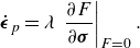 \begin{equation} \dot {\boldsymbol{\epsilon }}_p = \lambda \, \left. \frac {\partial F}{\partial \boldsymbol{\sigma }}\right |_{F = 0}. \end{equation}
Here, $\dot {\boldsymbol{\epsilon }}_p$
is the plastic rate-of-strain tensor and
$\dot {\boldsymbol{\epsilon }}_p$
is the plastic rate-of-strain tensor and $\lambda$
is a scalar that has to be determined as a part of the solution (Coon et al. Reference Coon, Maykut, Pritchard, Rothrock and Thorndike1974). We note that the plastic flow rule (1.1) can be arrived at using a variational argument (Howell, Kozyreff & Ockendon Reference Howell, Kozyreff and Ockendon2009).
$\lambda$
is a scalar that has to be determined as a part of the solution (Coon et al. Reference Coon, Maykut, Pritchard, Rothrock and Thorndike1974). We note that the plastic flow rule (1.1) can be arrived at using a variational argument (Howell, Kozyreff & Ockendon Reference Howell, Kozyreff and Ockendon2009).
The justifications provided for the elastic–plastic model are that (Coon et al. Reference Coon, Maykut, Pritchard, Rothrock and Thorndike1974): (i) during ridging/rafting of ice floes the work done against gravity, assuming no energy loss to friction, appears as the potential energy of the ridged/rafted floes, with the end result being independent of the rate at which ridging/rafting proceeds; and (ii) sea ice shares visual similarity with other materials that have been successfully modelled using plastic rheologies. Furthermore, Coon et al. (Reference Coon, Maykut, Pritchard, Rothrock and Thorndike1974) linked the yield function of the plastic response to the thickness distribution, thus coupling the rheology to the state of the ice cover. These ideas also led to the subsequent development of viscous–plastic (Hibler Reference Hibler1979) and elastic–viscous–plastic (Hunke & Dukowicz Reference Hunke and Dukowicz1997) models, which are some of the more widely used rheological models in current climate models (Keen et al. Reference Keen2021). This is because they are easier to implement numerically than the elastic–plastic model (Hibler Reference Hibler1979; Hunke & Dukowicz Reference Hunke and Dukowicz1997; Feltham Reference Feltham2008). More recently, anisotropic (Wilchinsky & Feltham Reference Wilchinsky and Feltham2004; Tsamados, Feltham & Wilchinsky Reference Tsamados, Feltham and Wilchinsky2013) and brittle (Girard et al. Reference Girard, Bouillon, Weiss, Amitrano, Fichefet and Legat2011; Bouillon & Rampal Reference Bouillon and Rampal2015; Dansereau et al. Reference Dansereau, Weiss, Saramito and Lattes2016; Ólason et al. Reference Ólason, Boutin, Korosov, Rampal, Williams, Kimmritz, Dansereau and Samaké2022) rheological models have been developed to capture some of the observed features in pack ice.
Results from these different rheological models have been compared with observations for fluctuations in sea ice extent (Agarwal & Wettlaufer Reference Agarwal and Wettlaufer2018), trends in sea ice drift and acceleration (Rampal et al. Reference Rampal, Weiss, Dubois and Campin2011) and linear kinematic features in pack ice (Bouchat et al. Reference Bouchat2022; Hutter et al. Reference Hutter2022). These studies show that the rheological models reproduce the observed features with mixed degrees of success.
From this discussion of the literature, it is clear that the focus of the past studies was either on floe-scale dynamics or on the development of rheological models. Although the development of viscous and plastic rheologies were motivated by the need to understand the consequences of floe–floe interactions on the dynamics at the continuum scale, any connection between the dynamics at these extreme scales remains tenuous. To our knowledge, there have been no attempts to systematically bridge the gap between these two scales. Hence, our goal here is to obtain the rheological properties of sea ice starting from the floe-scale dynamics. We achieve this using tools from statistical physics (Harris Reference Harris1971; Chapman & Cowling Reference Chapman and Cowling1990).
We begin by first constructing a mean-field description of the stochastic motion of a single floe. Our picture of the mean-field approximation of floe–floe interactions is analogous to that of a Brownian particle subjected to dry frictional force (Elmer Reference Elmer1997; de Gennes Reference de Gennes2005; Hayakawa Reference Hayakawa2005) in an external force field. The introduction of the dry (or Coulomb) friction, whose direction depends on the sign of the relative velocity of the floe with respect to the mean velocity, addresses the principal shortcoming of Sverdrup’s model (Sverdrup Reference Sverdrup1928). This approach allows us to obtain a generalised Fokker–Planck equation, also called the Kramers–Chandrasekhar equation (Kramers Reference Kramers1940; Chandrasekhar Reference Chandrasekhar1943), for the probability density function (PDF) of velocity fluctuations. We then obtain the continuum equations of motion through a Chapman–Enskog analysis (Lebowitz, Frisch & Helfand Reference Lebowitz, Frisch and Helfand1960; Chapman & Cowling Reference Chapman and Cowling1990) of this equation. In our case, the Newtonian rheology that emerges at large scales is a direct consequence of the dynamics at the floe scale.
The remainder of the paper is organised as follows. We begin in § 2 with the development of the stochastic model for the motion of an ice floe and obtain the kinetic equation for the PDF of its velocity. In § 3, we perform a Chapman–Enskog analysis of the kinetic equation and obtain the continuum equations of motion, including the rheological model that emerges from the floe-scale dynamics. Then, in § 4, we compare some of our results with observations and idealised large-scale simulations of ice drift, and then end with a summary of our study in § 5.
2. Stochastic drift of an ice floe
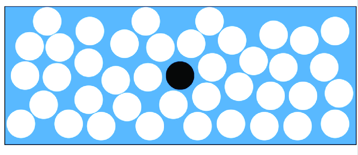
Here we consider the motion of a single floe and develop a mean field theory for its interactions with its neighbouring floes. For simplicity, we consider the ice floe to be a rigid circular disc with thickness $h$
and radius
$h$
and radius $R$
(see figure 1). In the region containing the floe, the ice concentration, which is defined as the fraction of the area of this region covered by ice, is
$R$
(see figure 1). In the region containing the floe, the ice concentration, which is defined as the fraction of the area of this region covered by ice, is $\mathcal{C}$
and the mean thickness of the ice cover is
$\mathcal{C}$
and the mean thickness of the ice cover is $\mathcal{H}$
. Apart from these bulk quantities, we ignore all other details – such as the geometry, thickness and floe size – of the neighbouring floes.
$\mathcal{H}$
. Apart from these bulk quantities, we ignore all other details – such as the geometry, thickness and floe size – of the neighbouring floes.
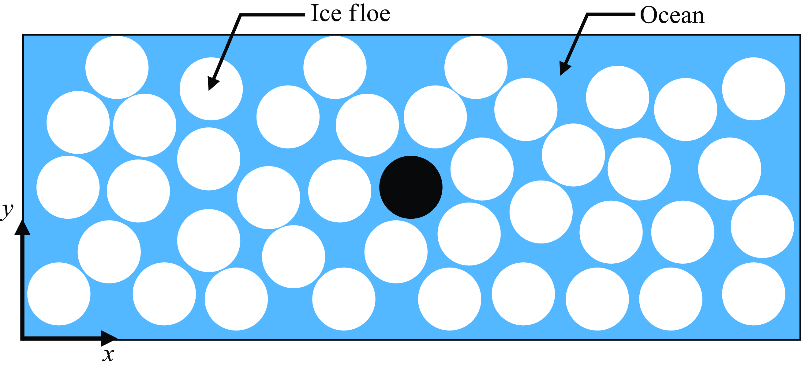
Figure 1. Schematic of the domain considered. The ice floe considered (in black) is assumed to be a circular disc with radius $R$
and thickness
$R$
and thickness $h$
. The ice concentration and the mean thickness in the region containing this floe are taken to be
$h$
. The ice concentration and the mean thickness in the region containing this floe are taken to be $\mathcal{C}$
and
$\mathcal{C}$
and $\mathcal{H}$
, respectively.
$\mathcal{H}$
, respectively.
2.1. Langevin equation
The equations governing the horizontal motion of the floe are
 \begin{equation} \frac {\mathrm{d} \boldsymbol{x}}{\mathrm{d}t} = \boldsymbol{v}, \end{equation}
and
 \begin{equation} \frac {\mathrm{d}}{\mathrm{d}t} \left (m \, \boldsymbol{v}\right ) = \boldsymbol{F}_a + \mathcal{B} \, \boldsymbol{\xi }(t) - \boldsymbol{F}_o + \boldsymbol{F}_G + \boldsymbol{F}_H - 2 \, m \, \Omega _0 \, \boldsymbol{k} \times \boldsymbol{v} - \mathcal{F} \, \boldsymbol{S}(\boldsymbol{v} - {\boldsymbol{u}}^{\infty }). \end{equation}
Here, $\boldsymbol{x} = (x,y)$
is the position vector,
$\boldsymbol{x} = (x,y)$
is the position vector, $\boldsymbol{v} = (u, v)$
is its two-dimensional velocity and
$\boldsymbol{v} = (u, v)$
is its two-dimensional velocity and $m$
is the mass of the ice floe. The wind forcing is separated into mean,
$m$
is the mass of the ice floe. The wind forcing is separated into mean, $\boldsymbol{F}_a(\boldsymbol{x},t)$
, and fluctuations,
$\boldsymbol{F}_a(\boldsymbol{x},t)$
, and fluctuations, $\mathcal{B} \, \boldsymbol{\xi (t)}$
, with
$\mathcal{B} \, \boldsymbol{\xi (t)}$
, with $\mathcal{B}$
being the amplitude of the fluctuations and
$\mathcal{B}$
being the amplitude of the fluctuations and $\boldsymbol{\xi (t)}$
being Gaussian white noise. The ocean drag force is represented by
$\boldsymbol{\xi (t)}$
being Gaussian white noise. The ocean drag force is represented by $\boldsymbol{F}_o(\boldsymbol{x},t)$
, which subsumes the contributions from skin friction and form drag (Steele, Morison & Untersteiner Reference Steele, Morison and Untersteiner1989). Forces due to gradients in the atmospheric pressure and sea surface height are represented by
$\boldsymbol{F}_o(\boldsymbol{x},t)$
, which subsumes the contributions from skin friction and form drag (Steele, Morison & Untersteiner Reference Steele, Morison and Untersteiner1989). Forces due to gradients in the atmospheric pressure and sea surface height are represented by $\boldsymbol{F}_G(\boldsymbol{x},t)$
and
$\boldsymbol{F}_G(\boldsymbol{x},t)$
and $\boldsymbol{F}_H(\boldsymbol{x},t)$
, respectively. The fourth term on the right-hand side of (2.2) represents the Coriolis force with
$\boldsymbol{F}_H(\boldsymbol{x},t)$
, respectively. The fourth term on the right-hand side of (2.2) represents the Coriolis force with $\Omega _0$
being the Coriolis frequency and
$\Omega _0$
being the Coriolis frequency and $\boldsymbol{k}$
the unit vector along the vertical. The last term represents the force on the floe that results from its interactions with the neighbouring floes. We model this force using Coulomb’s dry friction model (Elmer Reference Elmer1997);
$\boldsymbol{k}$
the unit vector along the vertical. The last term represents the force on the floe that results from its interactions with the neighbouring floes. We model this force using Coulomb’s dry friction model (Elmer Reference Elmer1997); $\mathcal{F} \equiv \mathcal{F}[g(\boldsymbol{x}, h, t)]$
represents the magnitude of the frictional force,
$\mathcal{F} \equiv \mathcal{F}[g(\boldsymbol{x}, h, t)]$
represents the magnitude of the frictional force, $g(\boldsymbol{x}, h, t)$
is the sea ice thickness distribution, and
$g(\boldsymbol{x}, h, t)$
is the sea ice thickness distribution, and $\boldsymbol{S}$
is a unit vector given by
$\boldsymbol{S}$
is a unit vector given by
 \begin{equation} \boldsymbol{S}(\boldsymbol{v} - {\boldsymbol{u}}^{\infty }) = \frac {\boldsymbol{v} - {\boldsymbol{u}}^{\infty }}{|\boldsymbol{v} - {\boldsymbol{u}}^{\infty }|}, \end{equation}
where ${\boldsymbol{u}}^{\infty }$
is the mean velocity. The function
${\boldsymbol{u}}^{\infty }$
is the mean velocity. The function $\boldsymbol{S}$
is a generalisation of the sign function for a two-dimensional vector. Introducing the fluctuating velocity as
$\boldsymbol{S}$
is a generalisation of the sign function for a two-dimensional vector. Introducing the fluctuating velocity as $\boldsymbol{v}^{\prime} = \boldsymbol{v} - {\boldsymbol{u}}^{\infty }$
, we write (2.3) as
$\boldsymbol{v}^{\prime} = \boldsymbol{v} - {\boldsymbol{u}}^{\infty }$
, we write (2.3) as
 \begin{equation} \boldsymbol{S}(\boldsymbol{v}^{\prime}) = \frac {\boldsymbol{v}^{\prime}}{|\boldsymbol{v}^{\prime}|}. \end{equation}
Here, we ignore any rotational motion of the floe caused by floe–floe interactions. The magnitude $\mathcal{F}$
represents the minimum force required to set the floe into motion starting from rest, and hence represents the threshold value of the frictional force. To establish the dependence of
$\mathcal{F}$
represents the minimum force required to set the floe into motion starting from rest, and hence represents the threshold value of the frictional force. To establish the dependence of $\mathcal{F}$
on
$\mathcal{F}$
on $g(\boldsymbol{x}, h,t)$
, we follow Hibler (Reference Hibler1979) and use the first two moments of
$g(\boldsymbol{x}, h,t)$
, we follow Hibler (Reference Hibler1979) and use the first two moments of $g(\boldsymbol{x}, h, t)$
, which are
$g(\boldsymbol{x}, h, t)$
, which are $\mathcal{C}$
and
$\mathcal{C}$
and $\mathcal{H}$
. In terms of
$\mathcal{H}$
. In terms of $g(\boldsymbol{x}, h, t)$
, these are given by (Toppaladoddi et al. Reference Toppaladoddi, Moon and Wettlaufer2023)
$g(\boldsymbol{x}, h, t)$
, these are given by (Toppaladoddi et al. Reference Toppaladoddi, Moon and Wettlaufer2023)
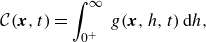 \begin{equation} \mathcal{C}(\boldsymbol{x},t) = \int _{0^+}^{\infty } \, g(\boldsymbol{x}, h, t) \, \mathrm{d}h, \end{equation}
and
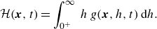 \begin{equation} \mathcal{H}(\boldsymbol{x},t) = \int _{0^+}^{\infty } \, h \, g(\boldsymbol{x}, h, t) \, \mathrm{d}h. \end{equation}
The dependence of $\mathcal{F}$
on
$\mathcal{F}$
on $\mathcal{C}$
and
$\mathcal{C}$
and $\mathcal{H}$
is determined by considering the following:
$\mathcal{H}$
is determined by considering the following:
-
(i) in the limits $\mathcal{C} \rightarrow 0$
and/or
$\mathcal{H} \rightarrow 0$
the interaction term should vanish as the ice cover vanishes;
$\mathcal{C} \rightarrow 0$
and/or
$\mathcal{H} \rightarrow 0$
the interaction term should vanish as the ice cover vanishes; -
(ii) as
$\mathcal{C} \rightarrow 1$
, the threshold force
$\mathcal{F}$
becomes independent of
$\mathcal{C}$
as the number of ice floes that could interact with the chosen floe saturates; -
(iii)
$\mathcal{F}$
should increase with increasing
$\mathcal{H}$
as the resistance offered by the neighbouring floes increases.


A functional form of $\mathcal{F}$
that satisfies these constraints is
$\mathcal{F}$
that satisfies these constraints is
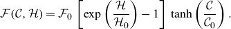 \begin{equation} \mathcal{F}(\mathcal{C}, \mathcal{H}) = \mathcal{F}_0 \, \left [\exp \left (\frac {\mathcal{H}}{\mathcal{H}_0}\right )-1\right ] \, \tanh \left (\frac {\mathcal{C}}{\mathcal{C}_0}\right ). \end{equation}
Here, $\mathcal{F}_0$
depends on ice strength and the amplitude of wind forcing, but for simplicity we assume it to be a constant;
$\mathcal{F}_0$
depends on ice strength and the amplitude of wind forcing, but for simplicity we assume it to be a constant; $\mathcal{H}_0$
is the equilibrium thickness which from observations is 1.5 m (Toppaladoddi & Wettlaufer Reference Toppaladoddi and Wettlaufer2015) and the value
$\mathcal{H}_0$
is the equilibrium thickness which from observations is 1.5 m (Toppaladoddi & Wettlaufer Reference Toppaladoddi and Wettlaufer2015) and the value $\mathcal{C}_0 = 0.3$
is chosen such that
$\mathcal{C}_0 = 0.3$
is chosen such that $\tanh (\mathcal{C}/\mathcal{C}_0 ) = 1$
for
$\tanh (\mathcal{C}/\mathcal{C}_0 ) = 1$
for $\mathcal{C} \geqslant 0.8$
. Figure 2 shows the qualitative behaviour of
$\mathcal{C} \geqslant 0.8$
. Figure 2 shows the qualitative behaviour of $\mathcal{F}$
with varying values of
$\mathcal{F}$
with varying values of $\mathcal{H}$
and
$\mathcal{H}$
and $\mathcal{C}$
. We should emphasise here that this functional form is not unique.
$\mathcal{C}$
. We should emphasise here that this functional form is not unique.
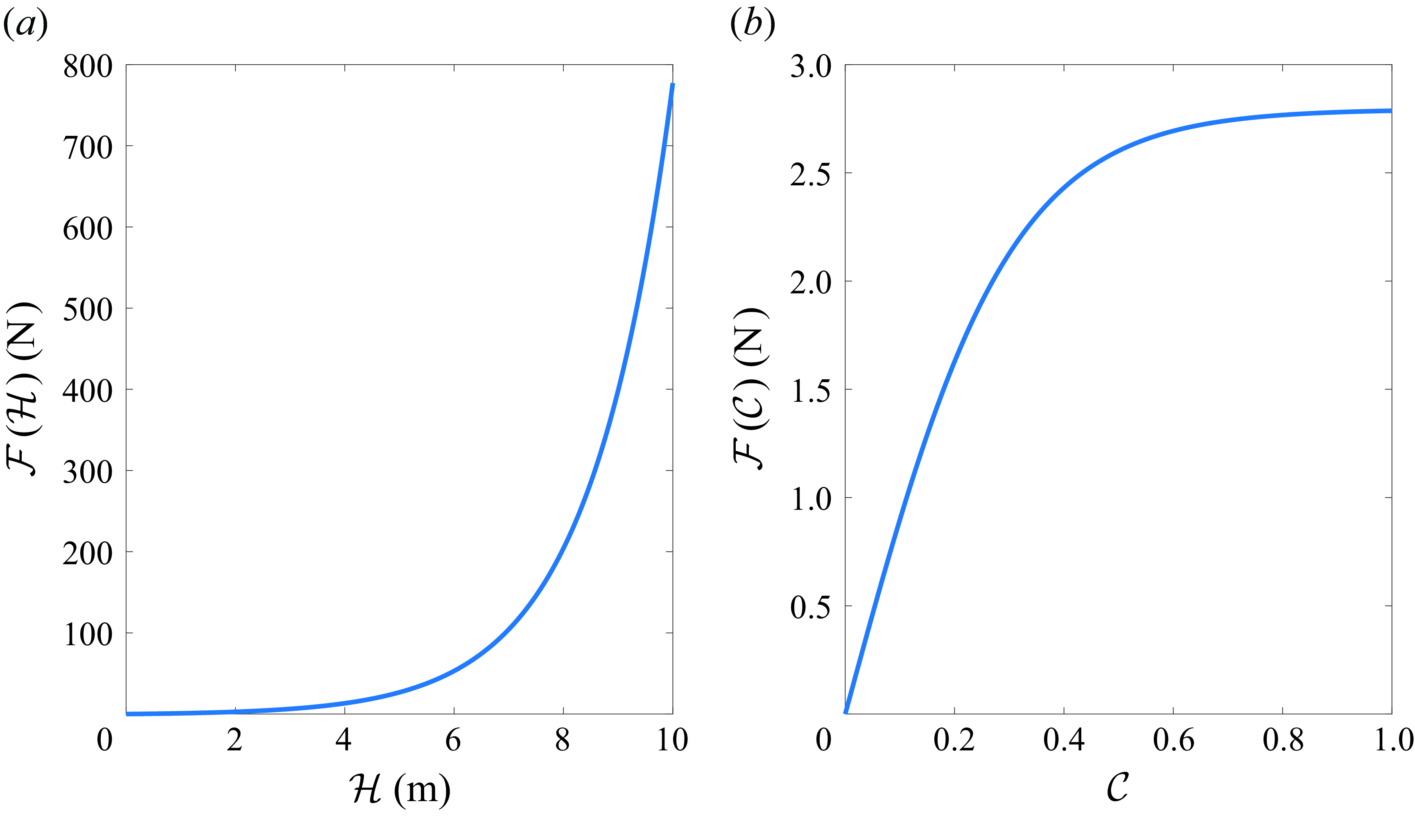
Figure 2. The qualitative behaviour of the threshold force $\mathcal{F}$
with varying values of (a) mean thickness (
$\mathcal{F}$
with varying values of (a) mean thickness ( $\mathcal{H}$
) and (b) concentration (
$\mathcal{H}$
) and (b) concentration ( $\mathcal{C}$
). In (a) the value of
$\mathcal{C}$
). In (a) the value of $\mathcal{C}$
is fixed to
$\mathcal{C}$
is fixed to $0.8$
, and in (b) the value of
$0.8$
, and in (b) the value of $\mathcal{H}$
is fixed to
$\mathcal{H}$
is fixed to $2$
m. The values of the other parameters are
$2$
m. The values of the other parameters are $\mathcal{F}_0 = 1$
N,
$\mathcal{F}_0 = 1$
N, $\mathcal{H}_0 = 1.5$
m and
$\mathcal{H}_0 = 1.5$
m and $\mathcal{C}_0 = 0.3$
.
$\mathcal{C}_0 = 0.3$
.
In introducing the floe–floe interaction term in (2.2), we have made the following assumptions: (i) (inelastic) collisions that involve only jostling and/or shearing between ice floes are important, and (ii) the role of collisions here is to drive the velocity to its mean value, ${\boldsymbol{u}}^{\infty }$
. On shorter time scales the motion of the ice floes is determined by wind forcing (Thorndike & Colony Reference Thorndike and Colony1982), which results in the different modes of interaction between ice floes discussed in § 1. Assumptions (i) and (ii) imply that only the shearing and jostling modes drive the system towards local equilibrium and the other two modes (rafting and ridging) do not. Hence, the rheology of the ice cover for large time and length scales will be determined by the shearing and jostling modes.
${\boldsymbol{u}}^{\infty }$
. On shorter time scales the motion of the ice floes is determined by wind forcing (Thorndike & Colony Reference Thorndike and Colony1982), which results in the different modes of interaction between ice floes discussed in § 1. Assumptions (i) and (ii) imply that only the shearing and jostling modes drive the system towards local equilibrium and the other two modes (rafting and ridging) do not. Hence, the rheology of the ice cover for large time and length scales will be determined by the shearing and jostling modes.
Our model can be justified using the following arguments. If $N (\gg 1)$
is the total number of floes, then any description of a single floe requires us to take into account its interactions with its
$N (\gg 1)$
is the total number of floes, then any description of a single floe requires us to take into account its interactions with its $n (\ll N)$
nearest neighbours. However, the construction of a system of coupled deterministic/stochastic differential equations for these localised interactions would also require us to take into account the interactions of the neighbouring floes with their own nearest neighbours. Hence, any description of the dynamics of a subset of the
$n (\ll N)$
nearest neighbours. However, the construction of a system of coupled deterministic/stochastic differential equations for these localised interactions would also require us to take into account the interactions of the neighbouring floes with their own nearest neighbours. Hence, any description of the dynamics of a subset of the $N$
floes leads to a closure problem, which is similar to the closure problem encountered in the kinetic theory of gases (Grad Reference Grad1958; Harris Reference Harris1971). Consequently, some assumptions would have to be made to truncate the problem. The mathematical form of the interactions in (2.2) represents a mean-field approximation of these interactions. This term embodies the fact that the collisions between the floe and its neighbours are due to the different velocities with which they move. However, if they all were to move with the mean velocity
$N$
floes leads to a closure problem, which is similar to the closure problem encountered in the kinetic theory of gases (Grad Reference Grad1958; Harris Reference Harris1971). Consequently, some assumptions would have to be made to truncate the problem. The mathematical form of the interactions in (2.2) represents a mean-field approximation of these interactions. This term embodies the fact that the collisions between the floe and its neighbours are due to the different velocities with which they move. However, if they all were to move with the mean velocity ${\boldsymbol{u}}^{\infty }$
then they would not collide with each other, in which case
${\boldsymbol{u}}^{\infty }$
then they would not collide with each other, in which case $\boldsymbol{S} = \boldsymbol{0}$
. It is important to highlight that the mathematical representation of the floe–floe interactions in (2.2) permits both acceleration and deceleration of the ice floe depending on the sign of the fluctuation.
$\boldsymbol{S} = \boldsymbol{0}$
. It is important to highlight that the mathematical representation of the floe–floe interactions in (2.2) permits both acceleration and deceleration of the ice floe depending on the sign of the fluctuation.
Assuming $m$
to be a constant, which implies the absence of thermal growth and ridging and rafting of ice floes, (2.2) becomes
$m$
to be a constant, which implies the absence of thermal growth and ridging and rafting of ice floes, (2.2) becomes
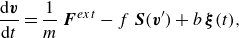 \begin{equation} \frac {\mathrm{d}\boldsymbol{v}}{\mathrm{d}t} = \frac {1}{m} \, {\boldsymbol{F}}^{ext} - f \, \boldsymbol{S}(\boldsymbol{v}^{\prime}) + b \, \boldsymbol{\xi }(t), \end{equation}
where ${\boldsymbol{F}}^{ext} = \boldsymbol{F}_a - \boldsymbol{F}_o + \boldsymbol{F}_G + \boldsymbol{F}_H - 2 \, m \, \Omega _0 \, \boldsymbol{k} \times \boldsymbol{v}$
,
${\boldsymbol{F}}^{ext} = \boldsymbol{F}_a - \boldsymbol{F}_o + \boldsymbol{F}_G + \boldsymbol{F}_H - 2 \, m \, \Omega _0 \, \boldsymbol{k} \times \boldsymbol{v}$
, $b = \mathcal{B}/m$
and
$b = \mathcal{B}/m$
and $f = \mathcal{F}/m$
. We are interested in the statistical properties of
$f = \mathcal{F}/m$
. We are interested in the statistical properties of $\boldsymbol{v}$
; but, unlike for the Langevin equation for the classical Brownian motion problem (Uhlenbeck & Ornstein Reference Uhlenbeck and Ornstein1930; Reif Reference Reif1965), it is difficult to solve (2.8) to obtain the moments of
$\boldsymbol{v}$
; but, unlike for the Langevin equation for the classical Brownian motion problem (Uhlenbeck & Ornstein Reference Uhlenbeck and Ornstein1930; Reif Reference Reif1965), it is difficult to solve (2.8) to obtain the moments of $\boldsymbol{v}$
because of the nonlinear function
$\boldsymbol{v}$
because of the nonlinear function $\boldsymbol{S}$
. For this reason, and for developing a continuum theory, we consider the PDF of
$\boldsymbol{S}$
. For this reason, and for developing a continuum theory, we consider the PDF of $\boldsymbol{v}$
.
$\boldsymbol{v}$
.
2.2. The Kramers-Chandrasekhar Equation (KCE)
The generalised Fokker–Planck equation or the KCE for the PDF, $\tilde {P}(\boldsymbol{x}, \boldsymbol{v},t)$
, corresponding to (2.8) is
$\tilde {P}(\boldsymbol{x}, \boldsymbol{v},t)$
, corresponding to (2.8) is
 \begin{equation} \frac {\partial \tilde {P}}{\partial t} + \boldsymbol{v} \cdot \nabla _{\boldsymbol{x}} \tilde {P} + \frac {{\boldsymbol{F}}^{ext}}{m} \cdot \nabla _{\boldsymbol{v}} \tilde {P} = \nabla _{\boldsymbol{v}} \cdot \{[f \, \boldsymbol{S}(\boldsymbol{v}^{\prime}) ] \, \tilde {P} + D \, \nabla _{\boldsymbol{v}} \tilde {P}\}. \end{equation}
Here, $\tilde {P}(\boldsymbol{x}, \boldsymbol{v},t) \, {\rm d}\boldsymbol{x} \, {\rm d}\boldsymbol{v}$
represents the probability that the floe’s velocity lies in the range
$\tilde {P}(\boldsymbol{x}, \boldsymbol{v},t) \, {\rm d}\boldsymbol{x} \, {\rm d}\boldsymbol{v}$
represents the probability that the floe’s velocity lies in the range $(\boldsymbol{v}, \boldsymbol{v}+{\rm d}\boldsymbol{v})$
and in a region
$(\boldsymbol{v}, \boldsymbol{v}+{\rm d}\boldsymbol{v})$
and in a region $(\boldsymbol{x}, \boldsymbol{x}+{\rm d}\boldsymbol{x})$
at time
$(\boldsymbol{x}, \boldsymbol{x}+{\rm d}\boldsymbol{x})$
at time $t$
,
$t$
, $\nabla _{\boldsymbol{x}}$
and
$\nabla _{\boldsymbol{x}}$
and $\nabla _{\boldsymbol{v}}$
are the gradient operators in physical and velocity spaces, respectively, and
$\nabla _{\boldsymbol{v}}$
are the gradient operators in physical and velocity spaces, respectively, and $D = b^2/2$
is the diffusion coefficient for diffusion of
$D = b^2/2$
is the diffusion coefficient for diffusion of $\tilde {P}$
in velocity space. The procedure for obtaining (2.10) using (2.8) is a standard one and is found elsewhere (Chandrasekhar Reference Chandrasekhar1943; Doering Reference Doering2018). We now introduce
$\tilde {P}$
in velocity space. The procedure for obtaining (2.10) using (2.8) is a standard one and is found elsewhere (Chandrasekhar Reference Chandrasekhar1943; Doering Reference Doering2018). We now introduce $\mathcal{P} = m \, N \, \tilde {P}$
, with
$\mathcal{P} = m \, N \, \tilde {P}$
, with $N$
being the total constant number of floes, such that
$N$
being the total constant number of floes, such that $\mathcal{P} \, {\rm d}\boldsymbol{x} \, {\rm d}\boldsymbol{v}$
gives the mass in the phase-space volume element
$\mathcal{P} \, {\rm d}\boldsymbol{x} \, {\rm d}\boldsymbol{v}$
gives the mass in the phase-space volume element ${\rm d}\boldsymbol{x} \, {\rm d}\boldsymbol{v}$
. To obtain the evolution equation for
${\rm d}\boldsymbol{x} \, {\rm d}\boldsymbol{v}$
. To obtain the evolution equation for $\mathcal{P}$
we multiply (2.9) with
$\mathcal{P}$
we multiply (2.9) with $m \, N$
, which gives
$m \, N$
, which gives
 \begin{equation} \frac {\partial \mathcal{P}}{\partial t} + \boldsymbol{v} \cdot \nabla _{\boldsymbol{x}} \mathcal{P} + \frac {{\boldsymbol{F}}^{ext}}{m} \cdot \nabla _{\boldsymbol{v}} \mathcal{P} = \nabla _{\boldsymbol{v}} \cdot \{ [f \, \boldsymbol{S}(\boldsymbol{v}^{\prime}) ] \, \mathcal{P} + D \, \nabla _{\boldsymbol{v}} \mathcal{P}\}. \end{equation}
Assuming the correlation time scale associated with the velocity fluctuations of the floe to be smaller than $\Omega _0^{-1}$
, we can neglect the Coriolis effect on the velocity fluctuations. This then leads to these fluctuations being isotropic. (We will test the veracity of this assumption by comparing our results with observations.) In addition, although the Coriolis force influences the route to equilibrium, the equilibrium solution itself should be independent of it. This is because the Coriolis force does not contribute to the relaxation of the system like the floe–floe collisions do. The Coriolis effect here is qualitatively similar to the effect of a weak magnetic field acting on a charged Brownian particle; the equilibrium PDF in this case is independent of the magnetic field (Wycoff & Balazs Reference Wycoff and Balazs1987). Hence, following Maxwell (Reference Maxwell1860), we conclude that the equilibrium PDF should be an even function of
$\Omega _0^{-1}$
, we can neglect the Coriolis effect on the velocity fluctuations. This then leads to these fluctuations being isotropic. (We will test the veracity of this assumption by comparing our results with observations.) In addition, although the Coriolis force influences the route to equilibrium, the equilibrium solution itself should be independent of it. This is because the Coriolis force does not contribute to the relaxation of the system like the floe–floe collisions do. The Coriolis effect here is qualitatively similar to the effect of a weak magnetic field acting on a charged Brownian particle; the equilibrium PDF in this case is independent of the magnetic field (Wycoff & Balazs Reference Wycoff and Balazs1987). Hence, following Maxwell (Reference Maxwell1860), we conclude that the equilibrium PDF should be an even function of $ (\boldsymbol{v}-{\boldsymbol{u}}^{\infty } )$
. However, contrary to Maxwell’s assumption (Maxwell Reference Maxwell1860), the fluctuations in
$ (\boldsymbol{v}-{\boldsymbol{u}}^{\infty } )$
. However, contrary to Maxwell’s assumption (Maxwell Reference Maxwell1860), the fluctuations in $u$
and
$u$
and $v$
are not independent because of the coupling through
$v$
are not independent because of the coupling through $\boldsymbol{S}(\boldsymbol{v}^{\prime})$
.
$\boldsymbol{S}(\boldsymbol{v}^{\prime})$
.
The macroscopic variables are now obtained as moments of $\mathcal{P}$
(Harris Reference Harris1971; Chapman & Cowling Reference Chapman and Cowling1990):
$\mathcal{P}$
(Harris Reference Harris1971; Chapman & Cowling Reference Chapman and Cowling1990):
-
(i) mass density,
(2.11)
\begin{equation} \rho (\boldsymbol{x}, t) = \int \! \mathcal{P}(\boldsymbol{x}, \boldsymbol{v},t) \, \mathrm{d}\boldsymbol{v}; \end{equation}
-
(ii) momentum density,
(2.12)
\begin{equation} \rho (\boldsymbol{x},t) \, {\boldsymbol{u}}^{\infty }(\boldsymbol{x},t) = \int \! \boldsymbol{v} \, \mathcal{P}(\boldsymbol{x}, \boldsymbol{v},t) \, \mathrm{d}\boldsymbol{v}; \end{equation}
-
(iii) energy density,
(2.13)
\begin{equation} \rho (\boldsymbol{x}, t) \, \mathcal{E}(\boldsymbol{x}, t) = \tfrac {1}{2} \, \int \! \left (\boldsymbol{v} - {\boldsymbol{u}}^{\infty }\right )^2 \, \mathcal{P}(\boldsymbol{x}, \boldsymbol{v},t) \, \mathrm{d} \boldsymbol{v}. \end{equation}


Here, $\rho$
denotes the mass density per unit area in the chosen region; it is, however, not related to the mass density of the ice floe itself, which has the units of mass per unit volume. In the case of a dilute gas, the kinetic energy associated with the velocity fluctuations (2.13), in/close to equilibrium, is related to the temperature of the gas (Harris Reference Harris1971; Chapman & Cowling Reference Chapman and Cowling1990; Lifshitz & Pitaevskii Reference Lifshitz and Pitaevskii2005). In our case, however, the velocity fluctuations do not have any thermodynamic significance.
$\rho$
denotes the mass density per unit area in the chosen region; it is, however, not related to the mass density of the ice floe itself, which has the units of mass per unit volume. In the case of a dilute gas, the kinetic energy associated with the velocity fluctuations (2.13), in/close to equilibrium, is related to the temperature of the gas (Harris Reference Harris1971; Chapman & Cowling Reference Chapman and Cowling1990; Lifshitz & Pitaevskii Reference Lifshitz and Pitaevskii2005). In our case, however, the velocity fluctuations do not have any thermodynamic significance.
3. The continuum theory
3.1. The macroscopic equations
As the macroscopic variables are obtained as moments of $\mathcal{P}$
((2.11)–(2.13)), the equations that govern their spatiotemporal evolution are obtained as appropriate moments of (2.10). To simplify the analysis, we make a change of variables from
$\mathcal{P}$
((2.11)–(2.13)), the equations that govern their spatiotemporal evolution are obtained as appropriate moments of (2.10). To simplify the analysis, we make a change of variables from $(\boldsymbol{x}_o, \boldsymbol{v}, t_o)$
to
$(\boldsymbol{x}_o, \boldsymbol{v}, t_o)$
to $(\boldsymbol{x}_n,\boldsymbol{v}^{\prime}, t_n)$
, where the subscripts ‘
$(\boldsymbol{x}_n,\boldsymbol{v}^{\prime}, t_n)$
, where the subscripts ‘ $o$
’ and ‘
$o$
’ and ‘ $n$
’ stand for old and new. Using
$n$
’ stand for old and new. Using $\boldsymbol{v} = {\boldsymbol{u}}^{\infty } + \boldsymbol{v}^{\prime}$
, we obtain the transformed differential operators as (Chapman & Cowling Reference Chapman and Cowling1990):
$\boldsymbol{v} = {\boldsymbol{u}}^{\infty } + \boldsymbol{v}^{\prime}$
, we obtain the transformed differential operators as (Chapman & Cowling Reference Chapman and Cowling1990):
-
(i) time derivative,
(3.1)
\begin{equation} \frac {\partial }{\partial t_o} = \frac {\partial }{\partial t_n} - \frac {\partial {\boldsymbol{u}}^{\infty }}{\partial t_n} \cdot \frac {\partial }{\partial \boldsymbol{v}^{\prime}}; \end{equation}
-
(ii) spatial gradient operator,
(3.2)
\begin{equation} \frac {\partial }{\partial \boldsymbol{x}_o} = \frac {\partial }{\partial \boldsymbol{x}_n} - \frac {\partial {\boldsymbol{u}}^{\infty }}{\partial \boldsymbol{x}_n} \cdot \frac {\partial }{\partial \boldsymbol{v}^{\prime}}; \end{equation}
-
(iii) velocity gradient operator,
(3.3)
\begin{equation} \frac {\partial }{\partial \boldsymbol{v}} = \frac {\partial }{\partial \boldsymbol{v}^{\prime}}. \end{equation}


Hence, the transformed KCE is
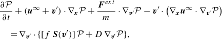 \begin{align} & \frac {\partial \mathcal{P}}{\partial t} + ({\boldsymbol{u}}^{\infty } + \boldsymbol{v}^{\prime}) \cdot \nabla _{\boldsymbol{x}} \mathcal{P} + \frac {{\boldsymbol{F}}^{ext}}{m} \cdot \nabla _{\boldsymbol{v}^{\prime}} \mathcal{P} - \boldsymbol{v}^{\prime} \cdot \left (\nabla _{\boldsymbol{x}} {\boldsymbol{u}}^{\infty } \cdot \nabla _{\boldsymbol{v}^{\prime}} \mathcal{P}\right ) \nonumber\\[8pt]&\quad = \nabla _{\boldsymbol{v}^{\prime}} \cdot \{ [f \, \boldsymbol{S}(\boldsymbol{v}^{\prime}) ] \, \mathcal{P} + D \, \nabla _{\boldsymbol{v}^{\prime}} \mathcal{P}\}, \end{align}
where the subscript ‘ $n$
’ has been dropped. The following macroscopic equations are obtained by multiplying (3.4) by
$n$
’ has been dropped. The following macroscopic equations are obtained by multiplying (3.4) by $1$
,
$1$
, $\boldsymbol{v}^{\prime}$
and
$\boldsymbol{v}^{\prime}$
and $v^{\prime 2}/2$
and integrating with respect to
$v^{\prime 2}/2$
and integrating with respect to $\boldsymbol{v}^{\prime}$
:
$\boldsymbol{v}^{\prime}$
:
-
(i) mass balance equation,
(3.5)
\begin{equation} \frac{\partial \rho}{\partial t} + \nabla_{\boldsymbol{x}} \cdot (\rho \, {\boldsymbol{u}}^{\infty}) = 0; \end{equation}
-
(ii) momentum balance equation,
(3.6)
\begin{equation} \frac{\mathcal{D} {\boldsymbol{u}}^{\infty}}{\mathcal{D}t} = \frac{1}{m} \, \left({\boldsymbol{F}}_a - {\boldsymbol{F}}_o + {\boldsymbol{F}}_G + {\boldsymbol{F}}_H \right) - 2 \, \Omega_0 \, {\boldsymbol{k}} \times {\boldsymbol{u}}^{\infty} + \frac{1}{\rho} \, \nabla_{\boldsymbol{x}} \cdot {\boldsymbol{\sigma}}, \end{equation}
where
(3.7)
\begin{equation} \frac {\mathcal{D}}{\mathcal{D}t} = \frac {\partial }{\partial t} + {\boldsymbol{u}}^{\infty } \cdot \nabla _{\boldsymbol{x}} \end{equation}
is the total derivative, and the stress tensor,
$\boldsymbol{\sigma }$
, is given by(3.8)
\begin{equation} \boldsymbol{\sigma }(\boldsymbol{x}, t) = -\int \, \boldsymbol{v}^{\prime} \, \boldsymbol{v}^{\prime} \, \mathcal{P}(\boldsymbol{x}, \boldsymbol{v}^{\prime}, t) \, \mathrm{d}\boldsymbol{v}^{\prime}, \end{equation}
which has the units of force per unit length;
-
(iii) energy balance equation,
(3.9)
\begin{align} \frac {\mathcal{D}}{\mathcal{D}t} \left (\rho \, \mathcal{E}\right ) + \rho \, \mathcal{E} \, \nabla _{\boldsymbol{x}} \cdot {\boldsymbol{u}}^{\infty } = - \nabla _{\boldsymbol{x}} \cdot \boldsymbol{\mathcal{Q}} - \boldsymbol{\sigma } : \nabla _{\boldsymbol{x}} {\boldsymbol{u}}^{\infty } + 2 \, \left (D - f \, \int \lvert \boldsymbol{v}^{\prime}\rvert \, \mathcal{P} \, \mathrm{d}\boldsymbol{v}^{\prime} \right ),\nonumber\\ \end{align}
where
$\lvert \boldsymbol{v}^{\prime}\rvert$
is the magnitude of
$\boldsymbol{v}^{\prime}$
, and(3.10)
\begin{equation} \mathcal{Q}(\boldsymbol{x}, t) = \tfrac {1}{2} \, \int \boldsymbol{v}^{\prime} \, v^{\prime 2} \, \mathcal{P}(\boldsymbol{x}, \boldsymbol{v}^{\prime}, t) \, \mathrm{d}\boldsymbol{v}^{\prime} \end{equation}
is the ‘heat flux’ vector.


Except for the last term in (3.9), these equations are similar to the ones that have been obtained for a dilute gas (Harris Reference Harris1971; Chapman & Cowling Reference Chapman and Cowling1990) and for non-interacting classical Brownian particles (Lebowitz et al. Reference Lebowitz, Frisch and Helfand1960; de Groot & Mazur Reference de Groot and Mazur2013). This term represents the difference between the energy input from the wind forcing and the frictional loss due to the inelastic collisions between the floe and its neighbours. Energy balance can be achieved by demanding that these two terms balance, but this would imply that the amplitude of fluctuations in wind forcing changes with the state of the ice cover. This is clearly unphysical; hence, these two terms in principle do not balance. Due to the lack of any thermodynamic significance of the velocity fluctuations, we shall not consider the energy balance equation any further.
To complete the momentum balance equation we have to evaluate the integral in (3.8) to determine $\boldsymbol{\sigma }$
, and to do this we need to solve the KCE (2.10).
$\boldsymbol{\sigma }$
, and to do this we need to solve the KCE (2.10).
3.2. Chapman–Enskog analysis
In order to obtain solutions to (2.10) using the Chapman–Enskog method (Lebowitz et al. Reference Lebowitz, Frisch and Helfand1960; Lifshitz & Pitaevskii Reference Lifshitz and Pitaevskii2005; de Groot & Mazur Reference de Groot and Mazur2013), we first make the equation dimensionless by choosing $R$
as the length scale,
$R$
as the length scale, $\Omega _0^{-1}$
as the time scale,
$\Omega _0^{-1}$
as the time scale, $R \, \Omega _0$
as the velocity scale and
$R \, \Omega _0$
as the velocity scale and $m/(\Omega _0^2 \, R^4)$
as the scale for
$m/(\Omega _0^2 \, R^4)$
as the scale for $\mathcal{P}$
. Using these, we get the dimensionless KCE to be
$\mathcal{P}$
. Using these, we get the dimensionless KCE to be
 \begin{equation} \frac {\partial \mathcal{P}_d}{\partial t_d} + \boldsymbol{v}_d \cdot \nabla _{\boldsymbol{x}_d} \mathcal{P}_d + {\boldsymbol{F}}^{ext}_d \cdot \nabla _{\boldsymbol{v}_d} \mathcal{P}_d = \frac {1}{\epsilon } \, \nabla _{\boldsymbol{v}_d} \cdot \left\{\mathcal{M} \, \boldsymbol{S}(\boldsymbol{v}^{\prime}_d) \, \mathcal{P}_d + \nabla _{\boldsymbol{v}_d} \mathcal{P}_d\right\}, \end{equation}
where the subscript $d$
denotes a dimensionless variable,
$d$
denotes a dimensionless variable, $\epsilon = \Omega _0^3 \, R^2/D$
, and
$\epsilon = \Omega _0^3 \, R^2/D$
, and $\mathcal{M} = (f \, R \, \Omega _0)/D$
is the dimensionless threshold force. As
$\mathcal{M} = (f \, R \, \Omega _0)/D$
is the dimensionless threshold force. As $\Omega _0 \sim 10^{-4}$
s
$\Omega _0 \sim 10^{-4}$
s $^{-1}$
,
$^{-1}$
, $R \sim 10^3$
m and
$R \sim 10^3$
m and $D \sim 1$
m
$D \sim 1$
m $^2$
s
$^2$
s $^{-3}$
, we have
$^{-3}$
, we have $\epsilon \ll 1$
. Using this small parameter we now expand
$\epsilon \ll 1$
. Using this small parameter we now expand $\mathcal{P}_d$
in a perturbative series
$\mathcal{P}_d$
in a perturbative series
 \begin{equation} \mathcal{P}_d = \mathcal{P}_d^{(0)} + \epsilon \, \mathcal{P}_d^{(1)} + \epsilon ^2 \, \mathcal{P}_d^{(2)} + \ldots , \end{equation}
where $\mathcal{P}^{(0)}_d$
is the local equilibrium distribution. We demand that
$\mathcal{P}^{(0)}_d$
is the local equilibrium distribution. We demand that
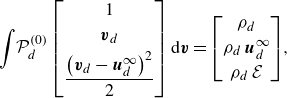 \begin{equation} \int \! \mathcal{P}^{(0)}_d \, { \begin{bmatrix} 1 \\[3pt] \boldsymbol{v}_d \\[3pt] \dfrac {\left (\boldsymbol{v}_d-\boldsymbol{u}^{\infty }_d\right )^2}{2} \end{bmatrix}} \, \mathrm{d}\boldsymbol{v}= { \begin{bmatrix} \rho _d \\[3pt] \rho _d \, \boldsymbol{u}^{\infty }_d \\[3pt] \rho _d \, \mathcal{E} \end{bmatrix}}, \end{equation}
and that the deviations from the local equilibrium distribution do not contribute to the macroscopic variables, i.e.
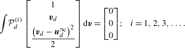 \begin{equation} \int \! \mathcal{P}^{(i)}_d \, { \begin{bmatrix} 1 \\[3pt] \boldsymbol{v}_d \\[3pt] \dfrac {\left (\boldsymbol{v}_d-\boldsymbol{u}^{\infty }_d\right )^2}{2} \end{bmatrix}} \, \mathrm{d}\boldsymbol{v}= { \begin{bmatrix} 0 \\[3pt] 0 \\[3pt] 0 \end{bmatrix}}; \hspace {0.25cm} i = 1, 2, 3, \ldots . \end{equation}
Using the expansion in (3.11) we get
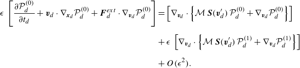 \begin{equation} \begin{aligned} \epsilon \, \left [\frac {\partial \mathcal{P}_d^{(0)}}{\partial t_d} + \boldsymbol{v}_d \cdot \nabla _{\boldsymbol{x}_d} \mathcal{P}_d^{(0)} + \boldsymbol{F}^{ext}_d \cdot \nabla _{\boldsymbol{v}_d} \mathcal{P}_d^{(0)} \right ] &= \left [\nabla _{\boldsymbol{v}_d} \cdot \left\{\mathcal{M} \, \boldsymbol{S}(\boldsymbol{v}^{\prime}_d) \, \mathcal{P}_d^{(0)} + \nabla _{\boldsymbol{v}_d} \mathcal{P}_d^{(0)}\right\}\right ] \\[6pt] &+ \epsilon \, \left [\nabla _{\boldsymbol{v}_d} \cdot \left\{\mathcal{M} \, \boldsymbol{S}(\boldsymbol{v}^{\prime}_d) \, \mathcal{P}_d^{(1)} + \nabla _{\boldsymbol{v}_d} \mathcal{P}_d^{(1)}\right\}\right ] \\[6pt] &+ O(\epsilon ^2). \end{aligned} \end{equation}
3.2.1. Calculation of
$\mathcal{P}_d^{(0)}$

Collecting terms of $O(1)$
gives
$O(1)$
gives
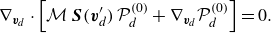 \begin{equation} \nabla _{\boldsymbol{v}_d} \cdot \left [\mathcal{M} \, \boldsymbol{S}(\boldsymbol{v}^{\prime}_d) \, \mathcal{P}_d^{(0)} + \nabla _{\boldsymbol{v}_d} \mathcal{P}_d^{(0)}\right ] = 0. \end{equation}
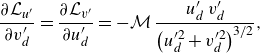
To solve this equation, we introduce the drift vector $\boldsymbol{\mathcal{L}}$
, which is defined as
$\boldsymbol{\mathcal{L}}$
, which is defined as
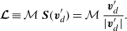 \begin{equation} \boldsymbol{\mathcal{L}} \equiv \mathcal{M} \, \boldsymbol{S}(\boldsymbol{v}^{\prime}_d) = \mathcal{M} \, \frac {\boldsymbol{v}^{\prime}_d}{|\boldsymbol{v}^{\prime}_d|}. \end{equation}
In component form, this is written as
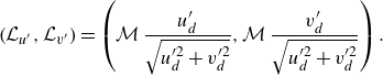 \begin{equation} \left (\mathcal{L}_{u^{\prime}}, \mathcal{L}_{v^{\prime}}\right ) = \left ( \mathcal{M} \, \frac {u^{\prime}_d}{\sqrt {u^{\prime 2}_d + v^{\prime 2}_d}}, \mathcal{M} \, \frac {v^{\prime}_d}{\sqrt {u^{\prime 2}_d + v^{\prime 2}_d}}\right ). \end{equation}
Using $\nabla _{\boldsymbol{v}_d} = \nabla _{\boldsymbol{v}^{\prime}_d}$
it is easily seen from (3.18) that
$\nabla _{\boldsymbol{v}_d} = \nabla _{\boldsymbol{v}^{\prime}_d}$
it is easily seen from (3.18) that
 \begin{equation} \frac {\partial \mathcal{L}_{u^{\prime}}}{\partial v^{\prime}_d} = \frac {\partial \mathcal{L}_{v^{\prime}}}{\partial u^{\prime}_d} = - \mathcal{M} \, \frac {u^{\prime}_d \, v^{\prime}_d}{\left (u^{\prime 2}_d+v^{\prime 2}_d\right )^{3/2}}, \end{equation}
which implies that $\boldsymbol{\mathcal{L}}$
can be expressed as the gradient of a potential, i.e.
$\boldsymbol{\mathcal{L}}$
can be expressed as the gradient of a potential, i.e. $\boldsymbol{\mathcal{L}} = \nabla _{\boldsymbol{v}^{\prime}_d} \Phi$
, and that the total probability flux vanishes everywhere (Risken Reference Risken1996). The required solution is readily found to be
$\boldsymbol{\mathcal{L}} = \nabla _{\boldsymbol{v}^{\prime}_d} \Phi$
, and that the total probability flux vanishes everywhere (Risken Reference Risken1996). The required solution is readily found to be
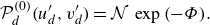 \begin{equation} \mathcal{P}^{(0)}_d\big(u^{\prime}_d,v^{\prime}_d\big) = \mathcal{N} \, \exp {\left (-\Phi \right )}. \end{equation}
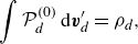
The integration constant $\mathcal{N}$
is determined by requiring that
$\mathcal{N}$
is determined by requiring that
 \begin{equation} \int \mathcal{P}^{(0)}_d \, \mathrm{d}\boldsymbol{v}^{\prime}_d = \rho _d, \end{equation}
where $\rho _d = \rho /(m/R^2)$
is the dimensionless mass density, and
$\rho _d = \rho /(m/R^2)$
is the dimensionless mass density, and
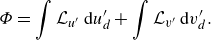 \begin{equation} \Phi = \int \mathcal{L}_{u^{\prime}} \, \mathrm{d}u^{\prime}_d + \int \mathcal{L}_{v^{\prime}} \, \mathrm{d}v^{\prime}_d. \end{equation}
Using (3.18) to evaluate the integrals, we get
 \begin{equation} \Phi = 2 \, \mathcal{M} \, \sqrt {u^{\prime 2}_d + v^{\prime 2}_d}, \end{equation}
which gives
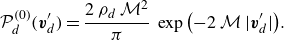 \begin{equation} \mathcal{P}^{(0)}_d(\boldsymbol{v}^{\prime}_d) = \frac {2 \, \rho _d \, \mathcal{M}^2}{\pi } \, \exp {\left (-2 \, \mathcal{M} \, |\boldsymbol{v}^{\prime}_d|\right )}. \end{equation}
The solution $\mathcal{P}^{(0)}_d$
represents the generalised Laplace distribution.
$\mathcal{P}^{(0)}_d$
represents the generalised Laplace distribution.
3.2.2. Calculation of
$\mathcal{P}_d^{(1)}$

Next, at $O(\epsilon )$
we have
$O(\epsilon )$
we have
 \begin{equation} \nabla _{\boldsymbol{v}_d} \cdot \left\{\mathcal{M} \, \boldsymbol{S}(\boldsymbol{v}^{\prime}_d) \, \mathcal{P}_d^{(1)} + \nabla _{\boldsymbol{v}_d} \mathcal{P}_d^{(1)}\right\} = \frac {\partial \mathcal{P}_d^{(0)}}{\partial t_d} + \boldsymbol{v}_d \cdot \nabla _{\boldsymbol{x}_d} \mathcal{P}_d^{(0)} + \boldsymbol{F}^{ext}_d \cdot \nabla _{\boldsymbol{v}_d} \mathcal{P}_d^{(0)}. \end{equation}
Using the solution (3.24) we evaluate the right-hand side of (3.25). To determine the time and spatial derivatives we note that the dependence of $\mathcal{P}^{(0)}_d$
on
$\mathcal{P}^{(0)}_d$
on $t$
and
$t$
and $\boldsymbol{x}$
is through the macroscopic variables. Hence, we get
$\boldsymbol{x}$
is through the macroscopic variables. Hence, we get
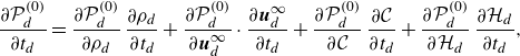 \begin{equation} \frac {\partial \mathcal{P}^{(0)}_d}{\partial t_d} = \frac {\partial \mathcal{P}^{(0)}_d}{\partial \rho _d} \, \frac {\partial \rho _d}{\partial t_d} + \frac {\partial \mathcal{P}^{(0)}_d}{\partial \boldsymbol{u}^{\infty }_d} \cdot \frac {\partial \boldsymbol{u}^{\infty }_d}{\partial t_d} + \frac {\partial \mathcal{P}^{(0)}_d}{\partial \mathcal{C}} \, \frac {\partial \mathcal{C}}{\partial t_d} + \frac {\partial \mathcal{P}^{(0)}_d}{\partial \mathcal{H}_d} \, \frac {\partial \mathcal{H}_d}{\partial t_d}, \end{equation}
and
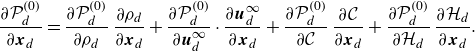 \begin{equation} \frac {\partial \mathcal{P}^{(0)}_d}{\partial \boldsymbol{x}_d} = \frac {\partial \mathcal{P}^{(0)}_d}{\partial \rho _d} \, \frac {\partial \rho _d}{\partial \boldsymbol{x}_d} + \frac {\partial \mathcal{P}^{(0)}_d}{\partial \boldsymbol{u}^{\infty }_d} \cdot \frac {\partial \boldsymbol{u}^{\infty }_d}{\partial \boldsymbol{x}_d} + \frac {\partial \mathcal{P}^{(0)}_d}{\partial \mathcal{C}} \, \frac {\partial \mathcal{C}}{\partial \boldsymbol{x}_d} + \frac {\partial \mathcal{P}^{(0)}_d}{\partial \mathcal{H}_d} \, \frac {\partial \mathcal{H}_d}{\partial \boldsymbol{x}_d}. \end{equation}
In the absence of thermal growth and ridging and rafting, the evolution equations for $\mathcal{C}$
and
$\mathcal{C}$
and $\mathcal{H}_d$
, where
$\mathcal{H}_d$
, where $\mathcal{H}_d = \mathcal{H}/R$
, are given by (cf. Hibler Reference Hibler1979)
$\mathcal{H}_d = \mathcal{H}/R$
, are given by (cf. Hibler Reference Hibler1979)
 \begin{equation} \frac {\partial \mathcal{C}}{\partial t_d} + \boldsymbol{v}_d \cdot \nabla _{\boldsymbol{x}_d} \mathcal{C} = 0, \end{equation}
and
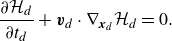 \begin{equation} \frac {\partial \mathcal{H}_d}{\partial t_d} + \boldsymbol{v}_d \cdot \nabla _{\boldsymbol{x}_d} \mathcal{H}_d = 0. \end{equation}
Using (3.5), (3.6), (3.28) and (3.29) to eliminate the time derivatives in (3.26) and combining all the terms on the right-hand side of (3.25) gives
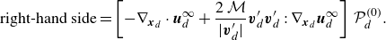 \begin{equation} \mathrm{right\text{-}hand\ side} = \left [-\nabla _{\boldsymbol{x}_d} \cdot \boldsymbol{u}^{\infty }_d + \frac {2 \, \mathcal{M}}{|\boldsymbol{v}^{\prime}_d|} \boldsymbol{v}^{\prime}_d \boldsymbol{v}^{\prime}_d : \nabla _{\boldsymbol{x}_d} \boldsymbol{u}^{\infty }_d\right ] \, \mathcal{P}^{(0)}_d. \end{equation}
In writing (3.30) we have omitted all terms that are linear in $\boldsymbol{v}^{\prime}_d$
because
$\boldsymbol{v}^{\prime}_d$
because
 \begin{equation} \int \! \boldsymbol{v}^{\prime}_d \, \mathcal{P}^{(0)}_d \, \mathrm{d}\boldsymbol{v}^{\prime}_d = 0. \end{equation}
Equation (3.30) suggests the functional form $\mathcal{P}^{(1)}_d = \mathcal{G} \, \mathcal{P}^{(0)}_d$
(Lebowitz et al. Reference Lebowitz, Frisch and Helfand1960; Lifshitz & Pitaevskii Reference Lifshitz and Pitaevskii2005), with
$\mathcal{P}^{(1)}_d = \mathcal{G} \, \mathcal{P}^{(0)}_d$
(Lebowitz et al. Reference Lebowitz, Frisch and Helfand1960; Lifshitz & Pitaevskii Reference Lifshitz and Pitaevskii2005), with
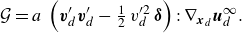 \begin{equation} \mathcal{G} = a \, \left (\boldsymbol{v}^{\prime}_d \boldsymbol{v}^{\prime}_d - \tfrac {1}{2} \, v^{\prime 2}_d \, \boldsymbol{\delta }\right ) : \nabla _{\boldsymbol{x}_d} \boldsymbol{u}^{\infty }_d. \end{equation}
Here, $a$
is a constant and
$a$
is a constant and $\boldsymbol{\delta }$
is the Kronecker delta. This form of
$\boldsymbol{\delta }$
is the Kronecker delta. This form of $\mathcal{P}^{(1)}_d$
also satisfies the constraints imposed in (3.14) (Lifshitz & Pitaevskii Reference Lifshitz and Pitaevskii2005). Using this in the left-hand side of (3.25) gives
$\mathcal{P}^{(1)}_d$
also satisfies the constraints imposed in (3.14) (Lifshitz & Pitaevskii Reference Lifshitz and Pitaevskii2005). Using this in the left-hand side of (3.25) gives
 \begin{equation} \mathrm{left\text{-}hand\ side} = \nabla _{\boldsymbol{v}_d} \cdot \left [\mathcal{P}^{(0)}_d\nabla _{\boldsymbol{v}_d} \mathcal{G}\right ]. \end{equation}
Evaluating the expression (3.33) and comparing it with (3.30), along with the observationally consistent (Agarwal & Wettlaufer Reference Agarwal and Wettlaufer2017) assumption that $\nabla _{\boldsymbol{x}_d} \cdot \boldsymbol{u}^{\infty }_d \approx 0$
, gives
$\nabla _{\boldsymbol{x}_d} \cdot \boldsymbol{u}^{\infty }_d \approx 0$
, gives $a = -1/2$
. Hence, the required solution is
$a = -1/2$
. Hence, the required solution is
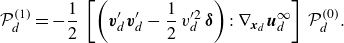 \begin{equation} \mathcal{P}^{(1)}_d = -\frac {1}{2} \, \left [\left (\boldsymbol{v}^{\prime}_d \boldsymbol{v}^{\prime}_d - \frac {1}{2} \, v^{\prime 2}_d \, \boldsymbol{\delta }\right ) : \nabla _{\boldsymbol{x}_d} \boldsymbol{u}^{\infty }_d\right ] \, \mathcal{P}^{(0)}_d. \end{equation}
3.3. The stress tensor
Now, in order to determine the stress tensor we revert to the dimensional forms of (3.24) and (3.34), as this makes it easier to obtain the rheological properties in dimensional form. These expressions are
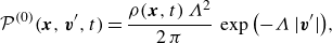 \begin{equation} \mathcal{P}^{(0)}(\boldsymbol{x}, \boldsymbol{v}^{\prime}, t) = \frac {\rho (\boldsymbol{x},t) \, \Lambda ^2}{2 \, \pi } \, \exp {\left (-\Lambda \, |\boldsymbol{v}^{\prime}|\right )}, \end{equation}
with $\Lambda = 2 \,f/D$
, and
$\Lambda = 2 \,f/D$
, and
 \begin{equation} \mathcal{P}^{(1)}(\boldsymbol{x}, \boldsymbol{v}^{\prime}, t) = -\frac {1}{2 \, D} \, \left [\left (\boldsymbol{v}^{\prime} \boldsymbol{v}^{\prime} - \frac {1}{2} \, v^{\prime 2} \, \boldsymbol{\delta }\right ) : \nabla _{\boldsymbol{x}} \boldsymbol{u}^{\infty }\right ] \, \mathcal{P}^{(0)}(\boldsymbol{x}, \boldsymbol{v}^{\prime}, t). \end{equation}
Using (3.8), we have (in index notation)
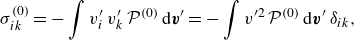 \begin{equation} \sigma ^{(0)}_{ik} = -\int \! \, v^{\prime}_i \, v^{\prime}_k \, \mathcal{P}^{(0)} \, \mathrm{d}\boldsymbol{v}^{\prime} = -\int \! \, v^{\prime 2} \, \mathcal{P}^{(0)} \, \mathrm{d}\boldsymbol{v}^{\prime} \, \delta _{ik}, \end{equation}
which gives
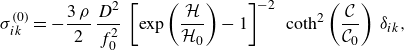 \begin{equation} \sigma ^{(0)}_{ik} = -\frac {3 \, \rho }{2} \, \frac {D^2}{f_0^2} \, \left [\exp \left (\frac {\mathcal{H}}{\mathcal{H}_0}\right ) - 1\right ]^{-2} \, \, \coth ^2\left (\frac {\mathcal{C}}{\mathcal{C}_0}\right ) \, \delta _{ik}, \end{equation}
where $f_0 = \mathcal{F}_0/m$
. This is the isotropic part of the stress tensor. We rewrite this expression as
$f_0 = \mathcal{F}_0/m$
. This is the isotropic part of the stress tensor. We rewrite this expression as
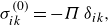 \begin{equation} \sigma ^{(0)}_{ik} = - \Pi \, \delta _{ik}, \end{equation}
where
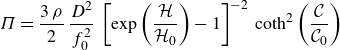 \begin{equation} \Pi = \frac {3 \, \rho }{2} \, \frac {D^2}{f_0^2} \, \left [\exp \left (\frac {\mathcal{H}}{\mathcal{H}_0}\right ) - 1\right ]^{-2} \, \coth ^2\left (\frac {\mathcal{C}}{\mathcal{C}_0}\right ) \end{equation}
is the pressure. Clearly, we have $\Pi \geqslant 0$
.
$\Pi \geqslant 0$
.
The deviatoric part of the stress tensor is given by
 \begin{equation} \sigma ^{(1)}_{ik} = -\int \! \, v^{\prime}_i \, v^{\prime}_k \, \mathcal{P}^{(1)} \, \mathrm{d}\boldsymbol{v}^{\prime} = \frac {1}{2 \, D} \, \frac {\partial u^{\infty }_m}{\partial x_n} \, \int \! \, v^{\prime}_i \, v^{\prime}_k \, \left [v^{\prime}_m \, v^{\prime}_n - \frac {1}{2} \, v^{\prime 2} \, \delta _{mn}\right ] \, \mathcal{P}^{(0)} \, \mathrm{d}\boldsymbol{v}^{\prime}. \end{equation}
Assuming sea ice to be an isotropic material, the integral in the above equation can be expressed in terms of only Kronecker deltas. The combination that on contraction with indices $m$
and
$m$
and $n$
gives zero is (Lifshitz & Pitaevskii Reference Lifshitz and Pitaevskii2005)
$n$
gives zero is (Lifshitz & Pitaevskii Reference Lifshitz and Pitaevskii2005)
 \begin{equation} \int \! \, v^{\prime}_i \, v^{\prime}_k \, \left [v^{\prime}_m \, v^{\prime}_n - \frac {1}{2} \, v^{\prime 2} \, \delta _{mn}\right ] \, \mathcal{P}^{(0)} \, \mathrm{d}\boldsymbol{v}^{\prime} = \mathcal{A} \, \left (\delta _{im} \, \delta _{kn} + \delta _{in} \, \delta _{km} - \delta _{ik} \, \delta _{mn}\right ). \end{equation}
The value of $\mathcal{A}$
is found by contracting indices
$\mathcal{A}$
is found by contracting indices $i$
and
$i$
and $m$
and
$m$
and $k$
and
$k$
and $n$
(Lifshitz & Pitaevskii Reference Lifshitz and Pitaevskii2005), which gives
$n$
(Lifshitz & Pitaevskii Reference Lifshitz and Pitaevskii2005), which gives
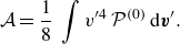 \begin{equation} \mathcal{A} = \frac {1}{8} \, \int \! \, v^{\prime 4} \, \mathcal{P}^{(0)} \, \mathrm{d}\boldsymbol{v}^{\prime}. \end{equation}
Hence,
 \begin{equation} \sigma ^{(1)}_{ik} = \frac {1}{16 \, D} \, \frac {\partial u^{\infty }_m}{\partial x_n} \, \left (\delta _{im} \, \delta _{kn} + \delta _{in} \, \delta _{km} - \delta _{ik} \, \delta _{mn}\right ) \, \int \! \, v^{\prime 4} \, \mathcal{P}^{(0)} \, \mathrm{d}\boldsymbol{v}^{\prime}. \end{equation}
Evaluating the integral finally leads to
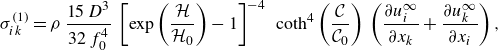 \begin{equation} \sigma ^{(1)}_{ik} = \rho \, \frac {15 \, D^3}{32 \, f_0^4} \, \left [\exp \left (\frac {\mathcal{H}}{\mathcal{H}_0}\right ) - 1\right ]^{-4} \, \, \coth ^4\left (\frac {\mathcal{C}}{\mathcal{C}_0}\right ) \, \left (\frac {\partial u^{\infty }_i}{\partial x_k} + \frac {\partial u^{\infty }_k}{\partial x_i}\right ), \end{equation}
where we have used $\nabla _{\boldsymbol{x}} \cdot \boldsymbol{u}^{\infty } \approx 0$
.
$\nabla _{\boldsymbol{x}} \cdot \boldsymbol{u}^{\infty } \approx 0$
.
The above equation can be written as
 \begin{equation} \sigma ^{(1)}_{ik} = \eta \, \dot {\gamma }_{ik}, \end{equation}
where
 \begin{equation} \eta = \rho \, \frac {15 \, D^3}{16 \, f_0^4} \, \left [\exp \left (\frac {\mathcal{H}}{\mathcal{H}_0}\right ) - 1\right ]^{-4} \, \coth ^4\left (\frac {\mathcal{C}}{\mathcal{C}_0}\right ) \end{equation}
is the dynamic shear viscosity of the ice cover, and
 \begin{equation} \dot {\gamma }_{ik} = \tfrac {1}{2} \, \left (\frac {\partial u^{\infty }_i}{\partial x_k} + \frac {\partial u^{\infty }_k}{\partial x_i}\right ) \end{equation}
is the rate-of-strain tensor. It is apparent that $\eta$
depends strongly on
$\eta$
depends strongly on $\mathcal{H}(\boldsymbol{x}, t)$
and
$\mathcal{H}(\boldsymbol{x}, t)$
and $\mathcal{C}({\boldsymbol{x}, t})$
. The momentum balance equation now becomes
$\mathcal{C}({\boldsymbol{x}, t})$
. The momentum balance equation now becomes
 \begin{equation} \frac {\mathcal{D}\boldsymbol{u}^{\infty }}{\mathcal{D}t} = -\frac {1}{\rho } \, \nabla _{\boldsymbol{x}} \Pi + \frac {1}{m} \, \left (\boldsymbol{F}_a - \boldsymbol{F}_o + \boldsymbol{F}_G + \boldsymbol{F}_H \right ) - 2 \, \Omega _0 \, \boldsymbol{k} \times \boldsymbol{u}^{\infty } + \frac {1}{\rho } \, \nabla _{\boldsymbol{x}} \cdot \left (\eta \, \boldsymbol{\dot {\gamma }}\right ). \end{equation}
This completes the development of our continuum theory.
4. Results
We shall now compare our theoretical results – both at the floe and continuum scales – with observations and simulations. Setting up and solving a canonical problem has, in our case, the disadvantage that there are no appropriate laboratory experiments to compare the results with. For this reason, we have to rely on results from observational data analyses (Rampal et al. Reference Rampal, Weiss, Marsan and Bourgoin2009) and large-scale simulations of sea ice circulation in the Arctic performed using Newtonian rheology (Rothrock Reference Rothrock1975a ).
4.1. Marginal distributions
We begin with the PDFs of velocity fluctuations. The marginal equilibrium distributions, $\mathcal{P}_{u^{\prime}}$
and
$\mathcal{P}_{u^{\prime}}$
and $\mathcal{P}_{v^{\prime}}$
, are obtained from the joint distribution (3.35) using
$\mathcal{P}_{v^{\prime}}$
, are obtained from the joint distribution (3.35) using
 \begin{equation} \mathcal{P}_{u^{\prime}} = \int _{-\infty }^{\infty } \! \mathcal{P}^{(0)}(u^{\prime},v^{\prime}) \, {\rm d}v^{\prime} = \frac {\rho \, \Lambda ^2}{2 \, \pi } \, \int _{-\infty }^{\infty } \! \exp {\left (-\Lambda \, \sqrt {u^{\prime 2} + v^{\prime 2}}\right )} \, \mathrm{d}v^{\prime}, \end{equation}
and
 \begin{equation} \mathcal{P}_{v^{\prime}} = \int _{-\infty }^{\infty } \! \mathcal{P}^{(0)}(u^{\prime},v^{\prime}) \, {\rm d}u^{\prime} = \frac {\rho \, \Lambda ^2}{2 \, \pi } \, \int _{-\infty }^{\infty } \! \exp {\left (-\Lambda \, \sqrt {u^{\prime 2} + v^{\prime 2}}\right )} \, \mathrm{d}u^{\prime}. \end{equation}
The integrals in (4.1) and (4.2) cannot be evaluated to give analytical expressions for $P_{u^{\prime}}$
and
$P_{u^{\prime}}$
and $P_{v^{\prime}}$
, so we determine them numerically. The components
$P_{v^{\prime}}$
, so we determine them numerically. The components $u^{\prime}$
and
$u^{\prime}$
and $v^{\prime}$
enter (3.24) as the fluctuating speed
$v^{\prime}$
enter (3.24) as the fluctuating speed $V^{\prime} = \sqrt {{u^{\prime2}} + {v^{\prime2}}}$
. This makes obtaining the PDF for the fluctuating speed,
$V^{\prime} = \sqrt {{u^{\prime2}} + {v^{\prime2}}}$
. This makes obtaining the PDF for the fluctuating speed, $\mathcal{P}_{V^{\prime}}$
, straightforward, which is found to be
$\mathcal{P}_{V^{\prime}}$
, straightforward, which is found to be
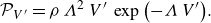 \begin{equation} \mathcal{P}_{V^{\prime}} = \rho \, \Lambda ^2 \, V^{\prime} \, \exp {\left (- \Lambda \, V^{\prime}\right )}. \end{equation}
For the purpose of comparing $\mathcal{P}_{u^{\prime}}$
,
$\mathcal{P}_{u^{\prime}}$
, $\mathcal{P}_{v^{\prime}}$
and
$\mathcal{P}_{v^{\prime}}$
and $\mathcal{P}_{V^{\prime}}$
with observations, we assume that
$\mathcal{P}_{V^{\prime}}$
with observations, we assume that $\rho$
is constant.
$\rho$
is constant.
We use results from the analysis of the International Arctic Buoy Program data by Rampal et al. (Reference Rampal, Weiss, Marsan and Bourgoin2009). A total of 450 drifters deployed between 1979 and 2001 were used, and data from only those buoys whose positions were at least 100 km away from the coasts were chosen. Rampal et al. (Reference Rampal, Weiss, Marsan and Bourgoin2009) chose a two-dimensional Cartesian coordinate system centred at the North Pole, with one of the axes pointing along the Greenwich meridian. For the analysis, the time period for winter was chosen from November to mid-May, and for summer from mid-June to mid-September. Further details on the procedure used to obtain the mean velocity, including the choice of length and time scales for averaging, and the velocity fluctuations can be found in Rampal et al. (Reference Rampal, Weiss, Marsan and Bourgoin2009).
In figure 3 we show the comparison between the theoretical PDF for the fluctuating speed and the observational PDF from Rampal et al. (Reference Rampal, Weiss, Marsan and Bourgoin2009). The functional form of the solution (4.3) is fit to the observational data, and $\rho$
and
$\rho$
and $\Lambda$
, which are the only fitting parameters, are determined from this fit. The values obtained are
$\Lambda$
, which are the only fitting parameters, are determined from this fit. The values obtained are $\rho = 0.94\,\rm g\,cm^{-2}$
and
$\rho = 0.94\,\rm g\,cm^{-2}$
and $\Lambda = 0.24$
(cm s−1)−1. The value of
$\Lambda = 0.24$
(cm s−1)−1. The value of $\rho$
obtained here is substantially smaller than the one used in the simulations of Rothrock (Reference Rothrock1975a
,Reference Rothrock
b
) (
$\rho$
obtained here is substantially smaller than the one used in the simulations of Rothrock (Reference Rothrock1975a
,Reference Rothrock
b
) ( $\rho = 300\,\rm g\,cm^{-2}$
).
$\rho = 300\,\rm g\,cm^{-2}$
).
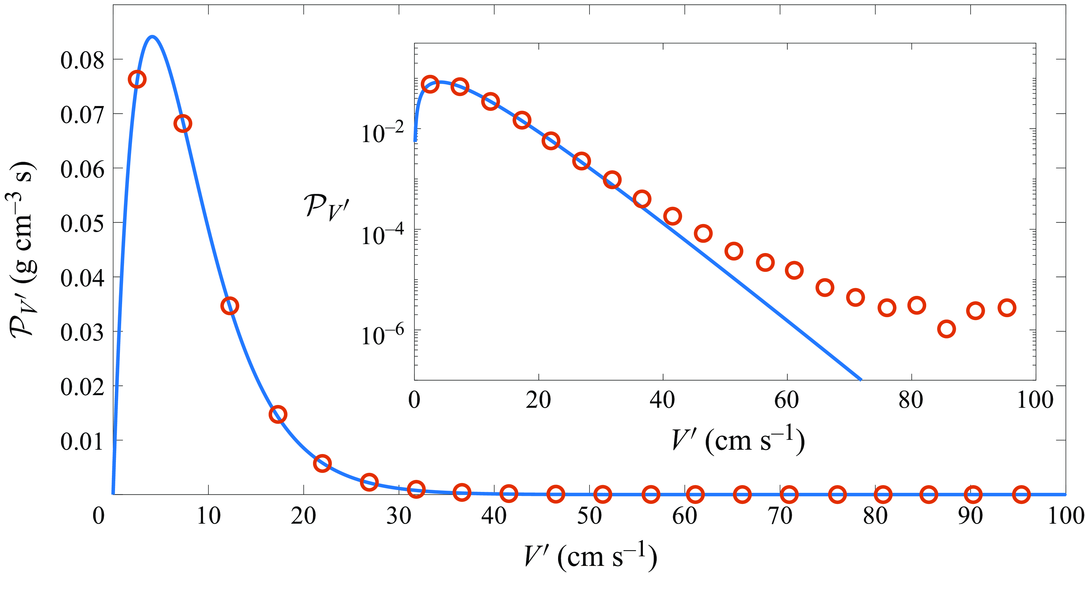
Figure 3. Comparison of our theoretical PDF for the fluctuating speed with observations. Circles are data from figure 10 in Rampal et al. (Reference Rampal, Weiss, Marsan and Bourgoin2009) and the solid curve is the functional form of the solution from theory (4.3). The value of $\rho$
and
$\rho$
and $\Lambda$
obtained from the fit are
$\Lambda$
obtained from the fit are $0.94\,\rm g\,cm^{-2}$
and
$0.94\,\rm g\,cm^{-2}$
and $0.238$
(cm s−1)−1, respectively. The inset shows the same figure in log–linear plot.
$0.238$
(cm s−1)−1, respectively. The inset shows the same figure in log–linear plot.
Using these values of $\rho$
and
$\rho$
and $\Lambda$
we compute the integral in (4.1) numerically to determine
$\Lambda$
we compute the integral in (4.1) numerically to determine $\mathcal{P}_{u^{\prime}}$
. Noting that
$\mathcal{P}_{u^{\prime}}$
. Noting that $\mathcal{P}_{u^{\prime}}$
and
$\mathcal{P}_{u^{\prime}}$
and $\mathcal{P}_{v^{\prime}}$
have the same functional forms (4.1) and (4.2), we compare
$\mathcal{P}_{v^{\prime}}$
have the same functional forms (4.1) and (4.2), we compare $\mathcal{P}_{u^{\prime}}$
with observations and find that
$\mathcal{P}_{u^{\prime}}$
with observations and find that $\mathcal{P}_{u^{\prime}}$
and
$\mathcal{P}_{u^{\prime}}$
and $\mathcal{P}_{v^{\prime}}$
for the velocity components are again Laplace distributions. This is shown in figure 4. As noted by Rampal et al. (Reference Rampal, Weiss, Marsan and Bourgoin2009), it is remarkable that the PDFs for
$\mathcal{P}_{v^{\prime}}$
for the velocity components are again Laplace distributions. This is shown in figure 4. As noted by Rampal et al. (Reference Rampal, Weiss, Marsan and Bourgoin2009), it is remarkable that the PDFs for $u^{\prime}$
and
$u^{\prime}$
and $v^{\prime}$
are approximately the same in each season, showing the fluctuations are isotropic and stationary.
$v^{\prime}$
are approximately the same in each season, showing the fluctuations are isotropic and stationary.
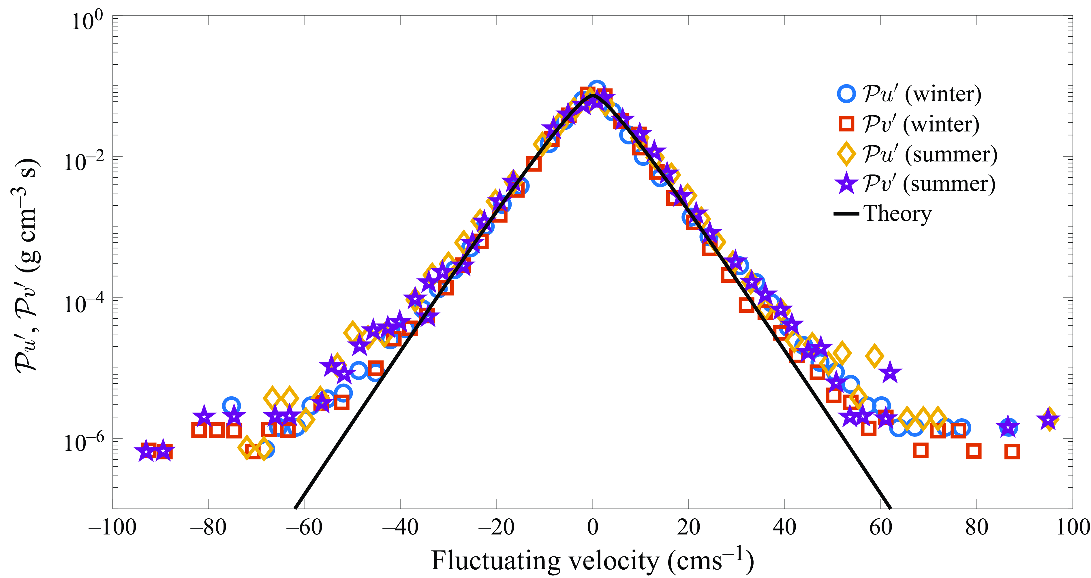
Figure 4. Comparison of our theoretical PDFs for ice velocity fluctuations with observations. Symbols are data from figure 9 in Rampal et al. (Reference Rampal, Weiss, Marsan and Bourgoin2009) and the solid curve is the PDF obtained from (4.1) after numerically evaluating the integral. The value of $\rho$
and
$\rho$
and $\Lambda$
used are
$\Lambda$
used are $0.94\,\rm g\,cm^{-2}$
and
$0.94\,\rm g\,cm^{-2}$
and $0.238$
(cm s
$0.238$
(cm s $^{-1}$
)−1, respectively (see figure 3).
$^{-1}$
)−1, respectively (see figure 3).
The agreement between theory and observations seen in figures 3 and 4 provides confidence in our mean field theory. The modelling of the floe–floe interactions using a Coulomb friction term makes the floe exhibit a stick-slip behaviour in its dynamics (Elmer Reference Elmer1997; de Gennes Reference de Gennes2005). This is similar in some aspects to the ‘crack-slip’ behaviour suggested by Thorndike (Reference Thorndike1986).
While the mean field theory has its advantages, it also has its limitations: the theory cannot explain the flattened tails in the PDF of speed (figure 3) and the marginal distributions (figure 4). One can speculate that this might be due to the advection of floes into a region of lower ice concentration or mean thickness or both. Incorporating such details when comparing results with observations is difficult. One can only infer the value of $f/D$
from the fit, but determining
$f/D$
from the fit, but determining $f$
and
$f$
and $D$
separately would require further analysis of the wind stress and ice field data to determine
$D$
separately would require further analysis of the wind stress and ice field data to determine $\mathcal{C}$
,
$\mathcal{C}$
, $\mathcal{H}$
and
$\mathcal{H}$
and $\mathcal{B}$
, which is beyond the scope of the current work.
$\mathcal{B}$
, which is beyond the scope of the current work.
4.2. Sea ice rheology
Some of the previously developed viscous models of sea ice did not contain a pressure term, with the challenge lying in relating the pressure to the state of the ice cover (Rothrock Reference Rothrock1970). Our approach allows us to determine explicitly the dependence of ice pressure and shear viscosity on the state of the ice cover. Here, we will explore these dependences in more detail.
In the limits $\mathcal{H} \rightarrow 0$
and/or
$\mathcal{H} \rightarrow 0$
and/or $\mathcal{C} \rightarrow 0$
both pressure,
$\mathcal{C} \rightarrow 0$
both pressure, $\Pi$
, and viscosity,
$\Pi$
, and viscosity, $\eta$
, diverge, which is unphysical. This is because the continuum theory is not valid in the limit of vanishing ice cover. However, the motion of isolated ice floes in this limit can still be studied using the kinetic theory developed in § 2. For this reason, we are interested in the dynamics of a near complete ice cover. We take
$\eta$
, diverge, which is unphysical. This is because the continuum theory is not valid in the limit of vanishing ice cover. However, the motion of isolated ice floes in this limit can still be studied using the kinetic theory developed in § 2. For this reason, we are interested in the dynamics of a near complete ice cover. We take $\mathcal{C} \in [0.8, 1 ]$
which gives
$\mathcal{C} \in [0.8, 1 ]$
which gives $\coth (\mathcal{C}/\mathcal{C}_0) = 1$
. Thus, the only relevant variable for the state of the ice cover now is
$\coth (\mathcal{C}/\mathcal{C}_0) = 1$
. Thus, the only relevant variable for the state of the ice cover now is $\mathcal{H}$
.
$\mathcal{H}$
.
4.2.1. Pressure
The pressure field in sea ice is now given by
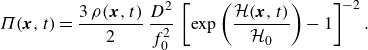 \begin{equation} \Pi (\boldsymbol{x},t) = \frac {3 \, \rho (\boldsymbol{x},t)}{2} \, \frac {D^2}{f_0^2} \, \left [\exp \left (\frac {\mathcal{H}(\boldsymbol{x},t)}{\mathcal{H}_0}\right ) - 1\right ]^{-2}. \end{equation}
It is seen that as $\mathcal{H}$
increases the pressure decreases, but it increases with increasing
$\mathcal{H}$
increases the pressure decreases, but it increases with increasing $\rho$
. This variation of
$\rho$
. This variation of $\Pi$
with
$\Pi$
with $\mathcal{H}$
is counterintuitive, but becomes clearer with the following, rather crude, analogy. In a dilute gas, the pressure in the gas (
$\mathcal{H}$
is counterintuitive, but becomes clearer with the following, rather crude, analogy. In a dilute gas, the pressure in the gas ( $\Pi _g$
) depends on the density (
$\Pi _g$
) depends on the density ( $\rho _g$
) and temperature (
$\rho _g$
) and temperature ( $T_g$
) of the gas as (Harris Reference Harris1971)
$T_g$
) of the gas as (Harris Reference Harris1971)
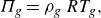 \begin{equation} \Pi _g = \rho _g \, R T_g, \end{equation}
which is the ideal gas law, with the gas constant $R$
. Comparing (4.5) and (4.4) we see that for a fixed
$R$
. Comparing (4.5) and (4.4) we see that for a fixed $D$
,
$D$
, $\mathcal{H}$
determines the mobility of sea ice – the smaller the value of
$\mathcal{H}$
determines the mobility of sea ice – the smaller the value of $\mathcal{H}$
the more mobile the ice floes are and hence larger the pressure will be because of increased number of collisions. Hence,
$\mathcal{H}$
the more mobile the ice floes are and hence larger the pressure will be because of increased number of collisions. Hence, $\mathcal{H}$
determines the pressure in sea ice like
$\mathcal{H}$
determines the pressure in sea ice like $T_g$
determines the pressure in an ideal gas. This analogy is apt only because of similar mechanisms of ‘microscopic’ interactions in a gas and sea ice: (elastic) collisions between molecules in the former and (inelastic) collisions between floes in the latter.
$T_g$
determines the pressure in an ideal gas. This analogy is apt only because of similar mechanisms of ‘microscopic’ interactions in a gas and sea ice: (elastic) collisions between molecules in the former and (inelastic) collisions between floes in the latter.
4.2.2. Shear viscosity
The kinematic viscosity of sea ice, $\nu = \eta /\rho$
, is
$\nu = \eta /\rho$
, is
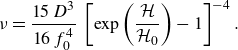 \begin{equation} \nu = \frac {15 \, D^3}{16 \, f_0^4} \, \left [\exp \left (\frac {\mathcal{H}}{\mathcal{H}_0}\right ) - 1\right ]^{-4}. \end{equation}
To highlight the dependence of $\nu$
on
$\nu$
on $\mathcal{H}$
we fix the constants
$\mathcal{H}$
we fix the constants $D = 1$
m
$D = 1$
m $^2$
s
$^2$
s $^{-3}$
and
$^{-3}$
and $f_0 = 1\,{\rm m}\,\rm s^{-2}$
. The variation in
$f_0 = 1\,{\rm m}\,\rm s^{-2}$
. The variation in $\nu$
with
$\nu$
with $\mathcal{H}$
is shown in figure 5. We see that
$\mathcal{H}$
is shown in figure 5. We see that $\nu$
varies by
$\nu$
varies by $O (10^{10} )$
as the mean thickness varies from
$O (10^{10} )$
as the mean thickness varies from $0.1$
to
$0.1$
to $5$
m. This behaviour is again explained using the analogy with a dilute gas, as an increased mobility at smaller
$5$
m. This behaviour is again explained using the analogy with a dilute gas, as an increased mobility at smaller $\mathcal{H}$
means larger momentum transfer between different regions.
$\mathcal{H}$
means larger momentum transfer between different regions.
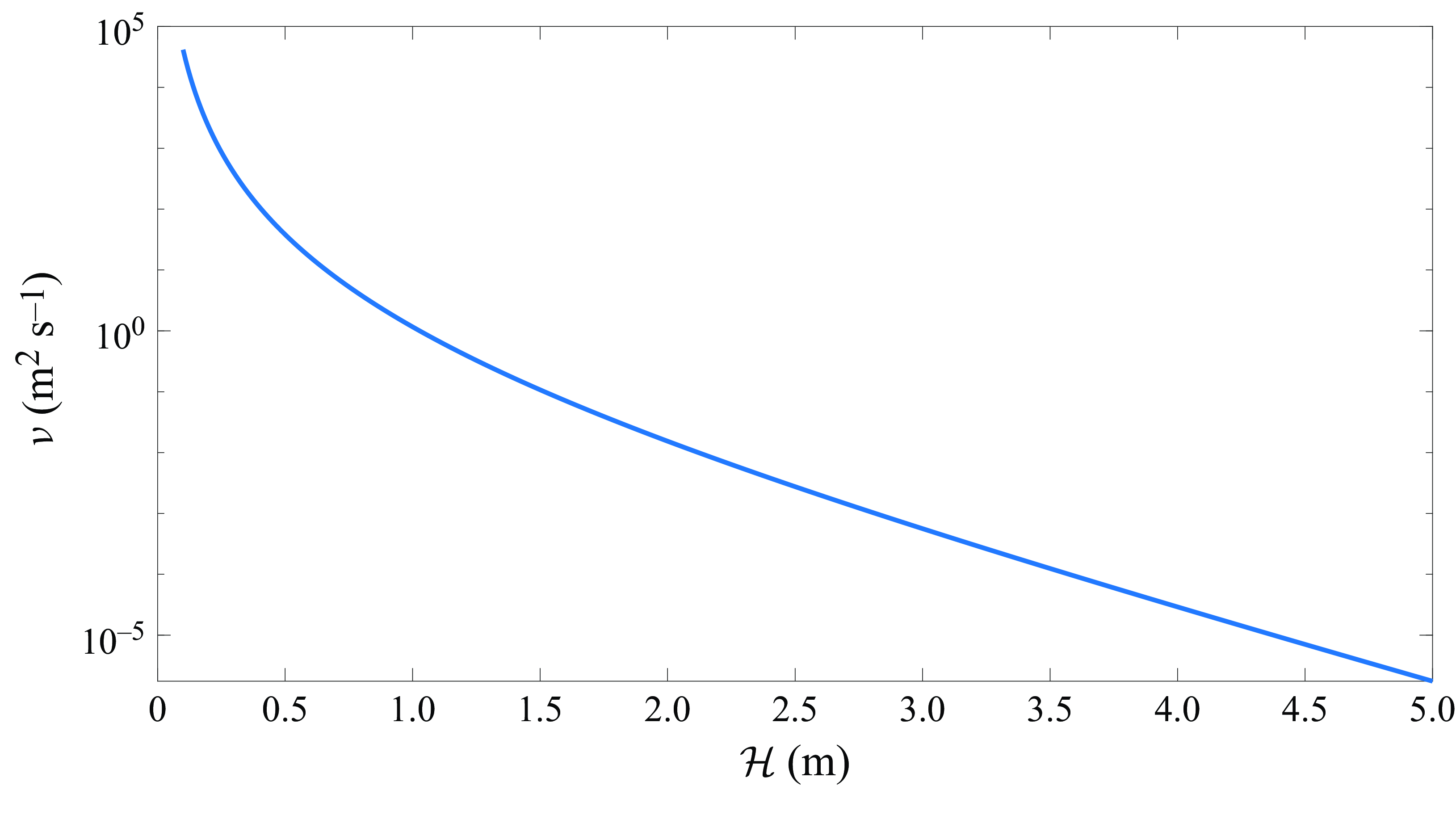
Figure 5. The dependence of kinematic viscosity, $\nu = \eta /\rho$
, on the mean thickness,
$\nu = \eta /\rho$
, on the mean thickness, $\mathcal{H}$
, based on the expression 4.6 for
$\mathcal{H}$
, based on the expression 4.6 for $D = 1$
m
$D = 1$
m $^2$
s
$^2$
s $^{-3}$
and
$^{-3}$
and $f_0 = 1\,\rm m\,s^{-2}$
.
$f_0 = 1\,\rm m\,s^{-2}$
.
In the Arctic basin, the mean thickness is larger closer to the boundaries of the basin because of ridging (Kwok et al. Reference Kwok, Cunningham, Wensnahan, Rigor, Zwally and Yi2009; Kwok & Cunningham Reference Kwok and Cunningham2015). Hence, the result from our theory implies that the viscosity of sea ice increases as one moves from the boundary regions to the interior of the basin. This explains why previous numerical studies found that a large value of shear viscosity, $\eta = 10^{12}\,\rm kg\,s^{-1}$
, was required to generate sufficient stresses in the interior of the basin, but a smaller value of
$\eta = 10^{12}\,\rm kg\,s^{-1}$
, was required to generate sufficient stresses in the interior of the basin, but a smaller value of $\eta = 6 \times 10^9\,\rm kg\,s^{-1}$
was required to observe realistic drift of sea ice and the formation of shear zones near the boundaries (Rothrock Reference Rothrock1975a
,Reference Rothrock
b
). This conflict over the choice of the value of
$\eta = 6 \times 10^9\,\rm kg\,s^{-1}$
was required to observe realistic drift of sea ice and the formation of shear zones near the boundaries (Rothrock Reference Rothrock1975a
,Reference Rothrock
b
). This conflict over the choice of the value of $\eta$
(or
$\eta$
(or $\nu$
) is resolved through its dependence on
$\nu$
) is resolved through its dependence on $\mathcal{H}$
, which has been found here. Hence, our theory is able to provide a qualitative explanation for the behaviour observed in the large-scale simulations, but a more detailed analysis of observational data are required to determine the quantitatively correct values of shear viscosity.
$\mathcal{H}$
, which has been found here. Hence, our theory is able to provide a qualitative explanation for the behaviour observed in the large-scale simulations, but a more detailed analysis of observational data are required to determine the quantitatively correct values of shear viscosity.
5. Summary and discussion
In summary, we have studied the motion of the Arctic sea ice cover at both the floe and continuum scales. We first considered the motion of a single ice floe and developed a mean field theory for its interactions with the neighbouring floes, neglecting phase change and ridging and rafting processes. The only variables used to represent the neighbouring floes were the ice concentration and the mean thickness. We assumed that only jostling and shearing modes of interaction drove the system towards local equilibrium and used a Coulomb friction term (Elmer Reference Elmer1997) to model the force resulting from these interactions. Using the Langevin equation for the floe velocity, we obtained the corresponding KCE for the PDF of the floe’s velocity. A Chapman–Enskog analysis of this equation led to the continuum equations of motion and a viscous rheology that emerged from the floe scale dynamics. The pressure in the ice cover and the shear viscosity were found to depend strongly on the mean thickness.
To compare our theory with observations, we obtained the marginal distributions and the PDF for the fluctuating speed of the floe. The marginal distributions were found to be the Laplace distribution, in good qualitative agreement with observations (Rampal et al. Reference Rampal, Weiss, Marsan and Bourgoin2009). We then placed our viscous model in the context of previous large-scale simulations of the ice cover (Rothrock Reference Rothrock1975a ) and were able to provide an explanation for some of the conflicting aspects of those studies. The qualitative agreement with observations and the large-scale simulations, despite the many simplifying assumptions made, provides confidence that our formulation of the problem is physically sound, and that the theory captures the leading-order physics associated with the motion of the ice cover.
An important aspect of the model that needs highlighting is that the interactions at the floe scale were modelled using a Coulomb friction term which is the simplest representation of plastic behaviour (Mellor Reference Mellor and Untersteiner2013): if the floe comes to rest, then there is a certain minimum force – given by the threshold $\mathcal{F}$
– that needs to be applied to the floe to set it in motion again. However, this plastic-like behaviour at the floe scale still leads to the viscous rheology in the continuum limit. Although the viscous models developed in the past could not determine the dependence of pressure and viscosity on the state of the ice cover, our approach allows us to do this. In building our model we assumed that the ice floes always existed, but this is not always the case. Under the action of wind and ocean stresses the continuous ice cover fractures into floes, and recent theoretical and modelling efforts have focussed on modelling this process (Girard et al. Reference Girard, Bouillon, Weiss, Amitrano, Fichefet and Legat2011; Bouillon & Rampal Reference Bouillon and Rampal2015; Dansereau et al. Reference Dansereau, Weiss, Saramito and Lattes2016). This suggests that the sea ice rheology on shorter time scales is perhaps the brittle rheology, but on much longer time scales it is viscous: the ice cover fractures into floes at shorter time scales (Asplin et al. Reference Asplin, Galley, Barber and Prinsenberg2012) and once the floes are produced the momentum transfer happens through shearing and jostling between the floes, as suggested by Reed & Campbell (Reference Reed and Campbell1962). This description provides a qualitative picture of the response of the ice cover over short and long time scales. However, this picture is not accurate during the early part of the freezing season when smaller floes coagulate to form larger floes and subsequently a continuous ice cover (Weeks & Ackley Reference Weeks and Ackley1986).
$\mathcal{F}$
– that needs to be applied to the floe to set it in motion again. However, this plastic-like behaviour at the floe scale still leads to the viscous rheology in the continuum limit. Although the viscous models developed in the past could not determine the dependence of pressure and viscosity on the state of the ice cover, our approach allows us to do this. In building our model we assumed that the ice floes always existed, but this is not always the case. Under the action of wind and ocean stresses the continuous ice cover fractures into floes, and recent theoretical and modelling efforts have focussed on modelling this process (Girard et al. Reference Girard, Bouillon, Weiss, Amitrano, Fichefet and Legat2011; Bouillon & Rampal Reference Bouillon and Rampal2015; Dansereau et al. Reference Dansereau, Weiss, Saramito and Lattes2016). This suggests that the sea ice rheology on shorter time scales is perhaps the brittle rheology, but on much longer time scales it is viscous: the ice cover fractures into floes at shorter time scales (Asplin et al. Reference Asplin, Galley, Barber and Prinsenberg2012) and once the floes are produced the momentum transfer happens through shearing and jostling between the floes, as suggested by Reed & Campbell (Reference Reed and Campbell1962). This description provides a qualitative picture of the response of the ice cover over short and long time scales. However, this picture is not accurate during the early part of the freezing season when smaller floes coagulate to form larger floes and subsequently a continuous ice cover (Weeks & Ackley Reference Weeks and Ackley1986).
The relative simplicity of our approach has both advantages and limitations. The first advantage is that from a detailed study of the motion of a single floe it is possible to obtain the large-scale behaviour of the ice cover. This provides an answer to one of the longstanding questions of how the rheological properties of a viscous model relate to the variables that quantify the state of the ice cover (Rothrock Reference Rothrock1975a ; Untersteiner Reference Untersteiner1986). The second advantage is that it allows for analytical tractability, which leads to the explicit continuum equations starting from the floe dynamics. The last advantage is that it provides unambiguous results, with only two free parameters, that can be compared with observations. This allows for the improvement of the model with relative ease when compared with most other models that do not have a similar floe-scale picture associated with them. Our theory also provides an observationally consistent framework to study the statistical properties of the ice velocity field, which would help in the development of simplified mathematical models of sea ice motion for incorporation into climate models.
The limitations of the theory are the following. First, the theory does not take into account the thermal growth and mechanical deformations of the ice floe. This is remedied by writing the mass of the ice floe as $m = \rho _i \, \pi \, R^2 \, h$
, where
$m = \rho _i \, \pi \, R^2 \, h$
, where $\rho _i$
is the constant density of the ice floe, and rewriting (2.2) as
$\rho _i$
is the constant density of the ice floe, and rewriting (2.2) as
 \begin{equation} m \, \frac {\mathrm{d} \boldsymbol{v}}{\mathrm{d}t} = - \boldsymbol{v} \, \frac {\mathrm{d}m}{\mathrm{d}t} + \boldsymbol{F}_a + \mathcal{B} \, \boldsymbol{\xi }(t) - \boldsymbol{F}_o + \boldsymbol{F}_G + \boldsymbol{F}_H - 2 \, m \, \Omega _0 \, \boldsymbol{k} \times \boldsymbol{v} - \mathcal{F} \, \boldsymbol{S}(\boldsymbol{v} - \boldsymbol{u}^{\infty }). \end{equation}
The changes in $R(t)$
and
$R(t)$
and $h(t)$
can now be coupled with the momentum equation (5.1). This, however, leads to a six-dimensional Fokker–Planck equation which is challenging to solve – both analytically and numerically. The second limitation is that some of the key parameters in the theory, such as
$h(t)$
can now be coupled with the momentum equation (5.1). This, however, leads to a six-dimensional Fokker–Planck equation which is challenging to solve – both analytically and numerically. The second limitation is that some of the key parameters in the theory, such as $D$
and
$D$
and $f_0$
, cannot be determined without a detailed analysis of observational data.
$f_0$
, cannot be determined without a detailed analysis of observational data.
These limitations, however, are not severe and can be overcome by solving the coupled stochastic differential equations for $\boldsymbol{v}$
and
$\boldsymbol{v}$
and $h$
and by performing a detailed, pan-Arctic analysis of wind stress and thickness distribution data. Our previous work on the thickness distribution of sea ice (Toppaladoddi & Wettlaufer Reference Toppaladoddi and Wettlaufer2015, Reference Toppaladoddi and Wettlaufer2017; Toppaladoddi et al. Reference Toppaladoddi, Moon and Wettlaufer2023) and our current theory provide a physical and mathematical framework to achieve this.
$h$
and by performing a detailed, pan-Arctic analysis of wind stress and thickness distribution data. Our previous work on the thickness distribution of sea ice (Toppaladoddi & Wettlaufer Reference Toppaladoddi and Wettlaufer2015, Reference Toppaladoddi and Wettlaufer2017; Toppaladoddi et al. Reference Toppaladoddi, Moon and Wettlaufer2023) and our current theory provide a physical and mathematical framework to achieve this.
Acknowledgements
The author thanks A.J. Wells for his critical comments on a previous version of the manuscript which were helpful in improving this work, and R.M.L. Evans, S.P. Thampi and K.V. Kumar for helpful discussions.
Declaration of interests
The author reports no conflict of interest.


 Open access