


1. Introduction
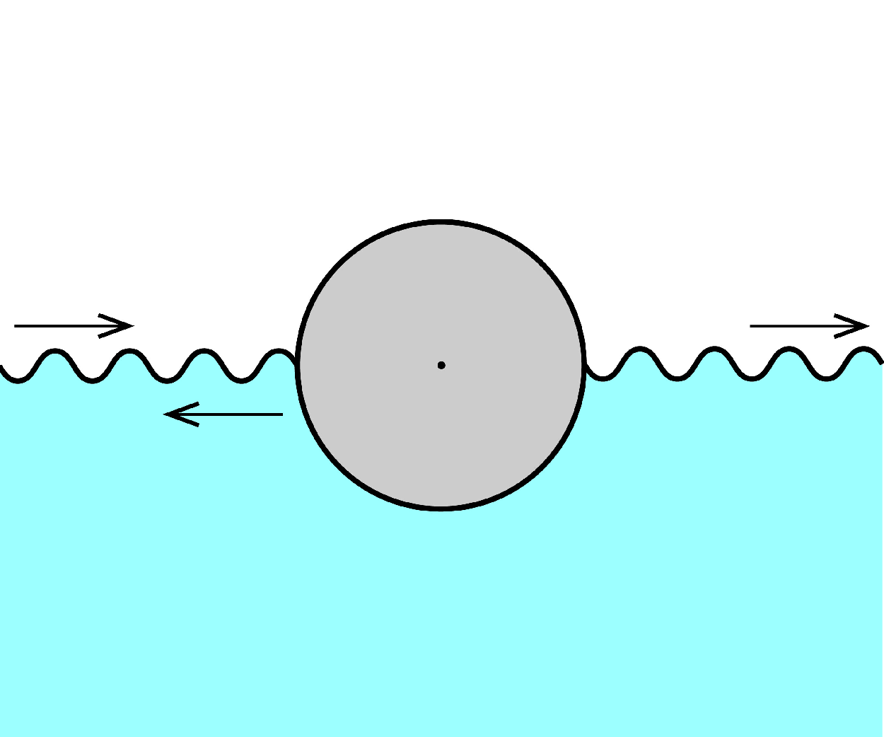
The scattering of surface waves by barriers on liquid surfaces is a classical problem in fluid mechanics, with applications in coastal engineering, fluid containment and wave energy systems. While scattering of gravity waves is typically observed in large-scale systems, scattering of capillary waves can occur in small-scale fluid systems. These systems often involve minimal surface-intersecting structures and have applications in laboratory set-ups, and in the control and containment of capillary liquids, such as the stabilisation of liquid globes by a wire loop (Pettit Reference Pettit2005), helical-wire-stabilised liquid cylinders (Lowry & Thiessen Reference Lowry and Thiessen2007), microstructured surfaces with pillars (Rothstein Reference Rothstein2010) and open capillary channels in biotechnology (Berthier et al. Reference Berthier, Dostie, Lee, Berthier and Theberge2019). Capillary–gravity surface waves arise where both gravity and surface tension influence wave dynamics. While extensive studies have investigated gravity wave scattering, studies of capillary–gravity wave scattering remain limited, either experimental measurements (Park, Liu & Chan Reference Park, Liu and Chan2012; Michel et al. Reference Michel, Pétrélis and Fauve2016; Wang, Liu & Zhang Reference Wang, Liu and Zhang2025) or theoretical analysis (Packham Reference Packham1968; Rhodes-Robinson Reference Rhodes-Robinson1982, Reference Rhodes-Robinson1996; Hocking Reference Hocking1987b ; Mahdmina & Hocking Reference Mahdmina and Hocking1990; Zhang & Thiessen Reference Zhang and Thiessen2013). In this paper, we develop a semi-analytical solution for the scattering of capillary–gravity waves by a fixed, semi-immersed cylindrical barrier (figure 1).
Theoretical analysis of capillary–gravity wave scattering is challenging due to the effect of surface tension, which raises the order of the surface boundary conditions (Hocking Reference Hocking1987a ; Henderson & Miles Reference Henderson and Miles1994) and requires an additional boundary condition at the contact lines – the three-phase junction where solid, liquid and gas meet (Jiang, Perlin & Schultz Reference Jiang, Perlin and Schultz2004; Nicolas Reference Nicolas2005; Kidambi Reference Kidambi2007; Huang et al. Reference Huang, Wolfe, Zhang and Zhong2020; Kim et al. Reference Kim, Moon and Kim2020). Accounting for contact line motion is crucial for accurately modelling the scattering and other capillary phenomena in various fluid configurations, such as sessile drops (Noblin, Buguin & Brochard-Wyart Reference Noblin, Buguin and Brochard-Wyart2004; Vukasinovic, Smith & Glezer Reference Vukasinovic, Smith and Glezer2007; Fayzrakhmanova & Straube Reference Fayzrakhmanova and Straube2009; Sharp Reference Sharp2012), bubbles (Harazi et al. Reference Harazi, Rupin, Stephan, Bossy and Marmottant2019), liquid bridges (Morse, Thiessen & Marston Reference Morse, Thiessen and Marston1996; Marr-Lyon, Thiessen & Marston Reference Marr-Lyon, Thiessen and Marston2001) and rivulets (Davis Reference Davis1980). Prior experimental studies have shown that both fixed and mobile contact lines influence the dynamics, such as selectively exciting standing wave patterns in Faraday wave resonances (Zhang et al. Reference Zhang, Borthwick and Lin2024), shifting the dispersion relation of travelling waves (Monsalve et al. Reference Monsalve, Maurel, Pagneux and Petitjeans2022) and significantly altering surface wave scattering by modifying the contact line conditions (Park et al. Reference Park, Liu and Chan2012; Michel et al. Reference Michel, Pétrélis and Fauve2016; Wang et al. Reference Wang, Liu and Zhang2025). The few previous theoretical analyses of capillary–gravity wave scattering with contact line conditions focused primarily on scattering from vertical cliffs (Rhodes-Robinson Reference Rhodes-Robinson1982), infinitesimally thin barriers (Hocking Reference Hocking1987b ; Rhodes-Robinson Reference Rhodes-Robinson1996; Zhang & Thiessen Reference Zhang and Thiessen2013), vertical cylinders (Mahdmina & Hocking Reference Mahdmina and Hocking1990) and porous plates (Gorgui, Faltas & Ahmed Reference Gorgui, Faltas and Ahmed1993; Rhodes-Robinson Reference Rhodes-Robinson1997; Chakrabarti & Sahoo Reference Chakrabarti and Sahoo1998).
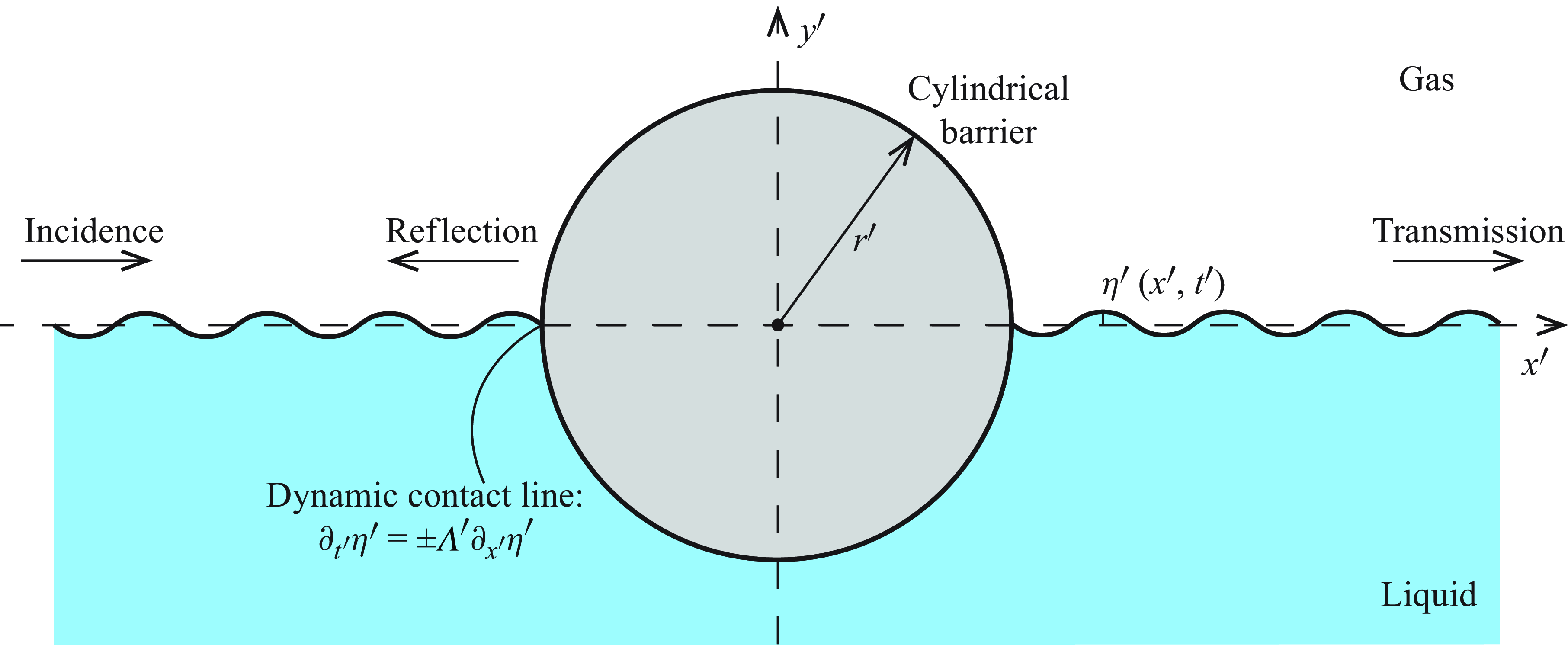
Figure 1. Schematic for capillary–gravity surface waves scattered by a fixed, semi-immersed, horizontal cylindrical barrier on a flat surface with a dynamic contact line given in (2.4).
In the absence of surface tension, the scattering of gravity waves by barriers has been a cornerstone of hydrodynamic research, with foundational studies by Dean (Reference Dean1945) and Ursell (Reference Ursell1947) providing critical insights into wave interactions with submerged and surface-piercing structures. Dean analysed the reflection of surface waves by a submerged plane barrier, while Ursell focused on the effect of a fixed vertical barrier on wave transmission and reflection in deep water, laying the groundwork for subsequent advancements. Built upon these seminal works, several studies were conducted between 1950 and 2000 to deepen the understanding of gravity wave scattering (Mei Reference Mei1989). Wehausen et al. (Reference Wehausen1960) provided a comprehensive review of surface waves, synthesising earlier findings, including those of Dean and Ursell. Classic work such as Newman (Reference Newman1965) analysed the propagation of gravity waves past a step bottom, providing foundational insights that continue to inform modern studies of wave scattering. Further studies, such as Liu & Abbaspour (Reference Liu and Abbaspour1982), employed the boundary integral equation method to investigate the scattering characteristics of gravity waves by vertical and inclined thin breakwaters, focusing on numerical solutions for reflection and transmission coefficients. Similarly, Sahoo, Lee & Chwang (Reference Sahoo, Lee and Chwang2000) examined wave trapping and generation by submerged vertical porous barriers, employing eigenfunction expansion and least-squares methods to analyse reflection coefficients, dynamic pressure distributions and wave amplitudes for various porous-effect parameters.
Recent research has extended these insights to more complex barrier designs, including porous, submerged and resonator-based configurations, with applications in wave energy dissipation and coastal protection. For instance, Chanda & Nandan Bora (Reference Chanda and Nandan Bora2022) investigated flexural–gravity wave interaction with submerged porous barriers under an ice-sheet modelled as a thin elastic plate, highlighting the influence of structural parameters on energy loss and wave forces. Chanda et al. (Reference Chanda, Barman, Sahoo and Meylan2024) explored flexural–gravity wave scattering by porous barriers in various configurations, introducing a scattering matrix to analyse mode conversion, Bragg resonance and energy dissipation. Manam & Kaligatla (Reference Manam and Kaligatla2014) used integral equations to compute reflection coefficients for membrane-coupled wave scattering by barriers with gaps, demonstrating the role of structural parameters in wave reflection. Lorenzo et al. (Reference Lorenzo, Pezzutto, De Lillo, Ventrella, De Vita, Bosia and Onorato2023) reported on a metamaterial-inspired wave attenuation device using submerged cylindrical pendula, showcasing resonance effects and Bragg scattering as mechanisms for significant energy dissipation and reflection. This evolving body of knowledge continues to inform the design of efficient and environmentally sustainable wave mitigation structures.
The study of surface wave scattering by cylindrical structures has been another cornerstone of hydrodynamic research, with applications in offshore engineering and wave energy management. A foundational work by Martin & Dixon (Reference Martin and Dixon1983) introduced a rigorous analytical framework to investigate gravity wave scattering by a semi-immersed fixed circular cylinder, highlighting the significance of diffraction effects and providing insights into reflection, transmission and hydrodynamic forces. Numerous studies have explored more complex systems, including floating cylinders (Porter & Evans Reference Porter and Evans2009), porous media (Zhuang, Zhao & Wan Reference Zhuang, Zhao and Wan2023) and metamaterial-based wave manipulation (Zheng, Liang & Greaves Reference Zheng, Liang and Greaves2024; Zhu et al. Reference Zhu, Zhao, Han, Zi, Hu and Chen2024). Recent advancements in computational methods, including high-fidelity numerical models, have provided insights into nonlinear wave–structure interactions, such as wave attenuation by floating breakwaters (Peng et al. Reference Peng, Lau, Wai and Chow2023). Complementary numerical investigations have further explored novel structural configurations for enhanced wave energy dissipation, analysing performance over a broad range of parameters (Panduranga & Koley Reference Panduranga and Koley2021).
The introduction of surface tension into wave scattering problems has been examined under diverse conditions including capillary–gravity wave scattering by surface tension gradient (Gou, Messiter & Schultz Reference Gou, Messiter and Schultz1993; Chou, Lucas & Stone Reference Chou, Lucas and Stone1995), by a non-uniform current (Trulsen & Mei Reference Trulsen and Mei1993), by surface convection zones (Kistovich & Chashechkin Reference Kistovich and Chashechkin2005), by a completely submerged porous elastic plate (Singh & Gayen Reference Singh and Gayen2022) and by bottom modulations (Mohapatra Reference Mohapatra2016; Meylan & Stepanyants Reference Meylan and Stepanyants2024). In these contexts, no structure intersects the free surface, so contact line effects do not arise. Scattering of capillary–gravity waves by surface-intersecting barriers with contact line effects was foundationally explored by Evans (Reference Evans1968), Packham (Reference Packham1968), Rhodes-Robinson (Reference Rhodes-Robinson1982, Reference Rhodes-Robinson1996), Hocking (Reference Hocking1987b ) and, more recently, Zhang & Thiessen (Reference Zhang and Thiessen2013). Evans and Packham examined the impact of surface tension on wave reflection by a vertical barrier, establishing critical edge conditions that have influenced subsequent studies. Rhodes-Robinson and Hocking independently investigated wave reflection using a linear dynamic contact line model following different approaches. Zhang & Thiessen (Reference Zhang and Thiessen2013) introduced dissipation models for capillary waves scattered through thin barriers, advancing the field’s understanding of capillary wave energy dissipation mechanisms at dynamic contact lines. Another related work by Mahdmina & Hocking (Reference Mahdmina and Hocking1990) analytically examined capillary–gravity wave scattering by a vertical cylinder using the same linear dynamic contact line model adopted here.
There are a few experimental investigations relevant to capillary–gravity wave scattering from barriers, particularly regarding the role of dynamic contact lines. Park et al. (Reference Park, Liu and Chan2012) investigated solitary wave reflection off vertical walls, using particle tracking velocimetry (PTV) to analyse the velocity field near the moving contact line. Their findings revealed complex flow phenomena, including surface rolling, boundary layer flow reversal, and the formation of jets and eddies near the meniscus. Michel et al. (Reference Michel, Pétrélis and Fauve2016) investigated the reflection of capillary–gravity surface waves by a plane vertical barrier, demonstrating that meniscus size significantly affects wave reflection – with a pinned contact line yielding nearly double the reflected energy compared with a fully developed meniscus – and introduced an acousto-optic-inspired acoustic measurement system to accurately measure wave amplitude, frequency and propagation direction. Wang et al. (Reference Wang, Liu and Zhang2025) performed experiments using acoustic measurements to quantify the effects of barrier depth, width and wave frequency on scattering, validating theoretical predictions of contact line dynamics in realistic fluid configurations and revealing the significant meniscus effect in capillary–gravity wave scattering.
Classical no-slip conditions lead to singular stresses, necessitating modified boundary conditions that better represent microscopic physics. Foundational works by Dussan (Reference Dussan1979) and others (Voinov Reference Voinov1976; Tanner Reference Tanner1979; De Gennes Reference de Gennes1985; Cox Reference Cox1986a ,Reference Cox b ) clarified that dynamic contact lines cannot be handled by classical slip-free models. Dynamics of contact lines can be modelled by the interplay between the apparent contact angle and contact-line velocity in the macroscopic regime, governing behaviours independent of microscopic complexities. We adopt a linearised dynamic contact line condition by Hocking (Reference Hocking1987b ) that bridges microscopic considerations with macroscopic wave behaviour by introducing an ‘effective-slip’ model. Hocking’s effective-slip model links the contact line velocity to the deviation of the contact angle from its equilibrium value, scaled by a slip coefficient with units of velocity. This slip coefficient encapsulates the interfacial properties of the solid–liquid boundary. At limiting extremes, a zero slip coefficient enforces ‘fixed’ contact lines, while an infinite slip coefficient ensures ‘free’ contact lines that maintain the contact angle with no energy dissipation. Between these extremes, finite slip coefficients produce boundary work as the contact line moves, converting a portion of wave energy into dissipation (Hocking Reference Hocking1987a ,Reference Hocking b ). The linear dynamic contact line model has been extensively used in analyses of various surface tension phenomena, such as behaviour of surface-wave damping in closed basins (Miles Reference Miles1967; Kidambi Reference Kidambi2009), oscillating droplets on solid plates (Lyubimov, Lyubimova & Shklyaev Reference Lyubimov, Lyubimova and Shklyaev2006) and forced oscillations of a cylindrical droplet bounded in the axial direction by rigid planes (Alabuzhev Reference Alabuzhev2016).
Our work aims to establish a milestone theoretical framework for surface wave scattering in fluid mechanics, by incorporating surface tension and a linear dynamic contact line condition into scattering of the waves by a cylindrical barrier with a non-zero cross-sectional dimension. While Hocking (Reference Hocking1987b ) included surface tension in the scattering but assumed an infinitesimal thin barrier, and Martin & Dixon (Reference Martin and Dixon1983) considered cylindrical barrier geometry but for gravity waves, the integration of both surface tension and cylindrical barrier geometry in our study has constituted a challenging problem in fluid mechanics. In the scattering problem considered by Mahdmina & Hocking (Reference Mahdmina and Hocking1990), a vertical cylinder geometry allows the wave field to be decomposed into an incident field plus a localised scattered field that vanishes at infinity. In our problem, however, a horizontally placed cylindrical barrier extends to infinity, rendering the scattered wave field (both transmitted and reflected components) unbounded, thus posing a more demanding analytical challenge.
Under the assumption of a linearised problem for an inviscid, incompressible and irrotational fluid, we employ techniques such as differential equations, conformal mapping and Fourier transforms to solve the coupled boundary value problems and formulate the entire problem as a compound integral equation problem. The resulting integral equations are simplified using integral equation techniques and numerically discretised via the Nyström method, enabling the computation of transmission and reflection coefficients of the scattered waves.
The paper is organised as follows. The linearised problem is formulated and divided into two boundary value problems (BVPs) in § 2. The two BVPs are solved and converted to coupled integral equations using conformal mapping and Fourier transform in § 3. The integral equations are combined and solved using even-odd separation in § 4. The validation of the model by comparing results with previous work in gravity waves is presented in § 5. The wave phase and spatial symmetry when no dissipation for capillary–gravity waves is addressed in § 6. The capillary–gravity wave scattering by an infinitesimal barrier is solved analytically using Fourier cosine and sine transform (FCT, FST) in § 7. The calculated results for fixed and free contact lines are presented in § 8 for barriers ranging from infinitesimal to having a finite cross-sectional dimension. The contact-line dissipation is addressed in § 9. All results are summarised and discussed in § 10.
2. Formulation: linearised problem and contact line model
The analysis begins by considering an equilibrium configuration where a horizontally placed cylindrical barrier of radius $r'$
is fixed and semi-immersed in an infinitely deep liquid (see figure 1). The infinitely deep liquid refers to the case when the liquid depth is much larger than the wavelength. A Cartesian coordinate system
$r'$
is fixed and semi-immersed in an infinitely deep liquid (see figure 1). The infinitely deep liquid refers to the case when the liquid depth is much larger than the wavelength. A Cartesian coordinate system $(x', y')$
is defined, with the origin located at the centre of the cylindrical barrier. The cylinder is uniformly extended along the third dimension
$(x', y')$
is defined, with the origin located at the centre of the cylindrical barrier. The cylinder is uniformly extended along the third dimension $z'$
, corresponding to the scenario that the cylinder length is much larger than the wavelength. The liquid, characterised by density
$z'$
, corresponding to the scenario that the cylinder length is much larger than the wavelength. The liquid, characterised by density $\rho$
, surface tension
$\rho$
, surface tension $\sigma$
and unperturbed pressure
$\sigma$
and unperturbed pressure $p_0' = P_0' - \rho g y'$
(
$p_0' = P_0' - \rho g y'$
( $P_0'$
is the atmospheric pressure), forms a static contact angle of
$P_0'$
is the atmospheric pressure), forms a static contact angle of $90^{\circ }$
with the barrier. This set-up is used to investigate the scattering of time-harmonic capillary–gravity waves – defined by angular frequency
$90^{\circ }$
with the barrier. This set-up is used to investigate the scattering of time-harmonic capillary–gravity waves – defined by angular frequency $\omega$
and wavenumber
$\omega$
and wavenumber $k$
– incident from
$k$
– incident from $x' \rightarrow -\infty$
.
$x' \rightarrow -\infty$
.
For an inviscid, incompressible and irrotational fluid, the fluid motion is governed by the continuity equation, the Navier–Stokes equation, alongside the kinematic and dynamic conditions at the free surface:
 \begin{align} \boldsymbol{\nabla }' \boldsymbol{\cdot } \boldsymbol{v}' & = 0, \qquad\qquad\qquad\! \forall (x', y') \in \Omega ', \\[-12pt] \nonumber \end{align}
 \begin{align} \partial _{t'} \boldsymbol{v}' + (\boldsymbol{v}' \boldsymbol{\cdot } \boldsymbol{\nabla }') \boldsymbol{v}' & = - \rho ^{-1} \boldsymbol{\nabla }' p', \qquad \forall (x', y') \in \Omega ', \\[-12pt] \nonumber \end{align}
 \begin{align} \partial _{t'} \eta ' + \boldsymbol{v}' \boldsymbol{\cdot } \boldsymbol{\nabla }' \eta ' & = \boldsymbol{\hat {n}}' \boldsymbol{\cdot } \boldsymbol{v}', \qquad\qquad \text{at } |x'| \gt r', y' = \eta ', \\[-12pt] \nonumber \end{align}
 \begin{align} p_0' + p' & = P_0' + \sigma \boldsymbol{\nabla }' \boldsymbol{\cdot } \boldsymbol{\hat {n}}', \quad \text{at } |x'| \gt r', y' = \eta ', \\[12pt] \nonumber \end{align}
where $\boldsymbol{v}' = \boldsymbol{v}'(x', y', t')$
is the velocity field,
$\boldsymbol{v}' = \boldsymbol{v}'(x', y', t')$
is the velocity field, $p' = p'(x', y', t')$
is the perturbed pressure of the wave field,
$p' = p'(x', y', t')$
is the perturbed pressure of the wave field, $\eta ' = \eta '(x', t')$
is the surface elevation with respect to its equilibrium position and
$\eta ' = \eta '(x', t')$
is the surface elevation with respect to its equilibrium position and $\Omega ' = \{(x', y') \in \mathbb{R}^2 \mid y' \lt 0 \text{ and } x^{\prime 2} + y^{\prime 2} \gt r^{\prime 2}\}$
defines the liquid domain. Here,
$\Omega ' = \{(x', y') \in \mathbb{R}^2 \mid y' \lt 0 \text{ and } x^{\prime 2} + y^{\prime 2} \gt r^{\prime 2}\}$
defines the liquid domain. Here, $\boldsymbol{\hat {n}}' = \boldsymbol{\nabla }'(y'-\eta ')/|\boldsymbol{\nabla }'(y'-\eta ')|$
is the normal vector of the free surface pointing outward of the liquid domain and
$\boldsymbol{\hat {n}}' = \boldsymbol{\nabla }'(y'-\eta ')/|\boldsymbol{\nabla }'(y'-\eta ')|$
is the normal vector of the free surface pointing outward of the liquid domain and $\boldsymbol{\nabla }' \boldsymbol{\cdot } \boldsymbol{\hat {n}}'$
represents the curvature of the free surface.
$\boldsymbol{\nabla }' \boldsymbol{\cdot } \boldsymbol{\hat {n}}'$
represents the curvature of the free surface.
Introducing the velocity potential with $\boldsymbol{v}' = \boldsymbol{\nabla }' \phi '$
and considering a linearised problem, (2.1) simplifies to
$\boldsymbol{v}' = \boldsymbol{\nabla }' \phi '$
and considering a linearised problem, (2.1) simplifies to
 \begin{align} \nabla ^{\prime 2} \phi ' & = 0, \qquad\qquad\qquad\quad \forall (x', y') \in \Omega ', \\[-12pt] \nonumber \end{align}
 \begin{align} \partial _{t'} \phi ' & = - p' / \rho , \qquad\qquad\,\,\,\, \forall (x', y') \in \Omega ', \\[-12pt] \nonumber \end{align}
 \begin{align} \partial _{y'} \phi ' & = \partial _{t'} \eta ' , \qquad\qquad\qquad\! \text{at } |x'| \gt r', y' = 0, \\[-12pt] \nonumber \end{align}
 \begin{align} p' & = - \sigma \partial _{x'}^2 \eta ' + \rho g \eta ' , \quad \text{at } |x'| \gt r', y' = 0. \\[12pt] \nonumber \end{align}
To ensure the validity of the linearisation, we assume that the perturbation from the equilibrium configuration is small. Specifically, the surface elevation $\eta '$
must satisfy
$\eta '$
must satisfy $k \eta ' \ll 1$
.
$k \eta ' \ll 1$
.
In addition, the problem has to be solved subject to the non-penetration condition at the barrier:
 \begin{equation} \boldsymbol{\hat {n}}' \boldsymbol{\cdot } \boldsymbol{\nabla }' \phi ' = 0, \qquad \text{at } |x'| \lt r', y' = - \sqrt {r^{\prime 2} - x^{\prime 2}}, \end{equation}
where $\boldsymbol{\hat {n}}'$
represents the normal vector at the cylindrical barrier surface.
$\boldsymbol{\hat {n}}'$
represents the normal vector at the cylindrical barrier surface.
The edge conditions imposed on $\eta '$
at the three-phase junction are given by the linear dynamic contact line condition from Hocking (Reference Hocking1987b
):
$\eta '$
at the three-phase junction are given by the linear dynamic contact line condition from Hocking (Reference Hocking1987b
):
 \begin{equation} \partial _{t'} \eta ' = \pm \Lambda ' \partial _{x'} \eta ', \qquad \text{at } x' = \pm r', \end{equation}
where the slip coefficient $\Lambda '$
has dimensions of velocity and is taken to be a non-negative real-valued constant. The plus and minus signs correspond to the right and left sides of the barrier, respectively.
$\Lambda '$
has dimensions of velocity and is taken to be a non-negative real-valued constant. The plus and minus signs correspond to the right and left sides of the barrier, respectively.
The imposed edge condition given in (2.4) governs the contact line’s behaviour via the slip coefficient $\Lambda '$
. The condition includes two special cases as its extremes: When
$\Lambda '$
. The condition includes two special cases as its extremes: When $\Lambda ' = 0$
, the contact line is effectively fixed (i.e.
$\Lambda ' = 0$
, the contact line is effectively fixed (i.e. $\partial _{t'}\eta ' = 0$
), termed as ‘fixed’ contact lines; conversely, as
$\partial _{t'}\eta ' = 0$
), termed as ‘fixed’ contact lines; conversely, as $\Lambda ' \to \infty$
, the contact line becomes completely free to slide while maintaining a constant contact angle which is
$\Lambda ' \to \infty$
, the contact line becomes completely free to slide while maintaining a constant contact angle which is $90^\circ$
here (i.e.
$90^\circ$
here (i.e. $\partial _{x'} \eta ' = 0$
), termed as ‘free’ contact lines. There is no energy dissipation in these two extremes. Intermediate values of
$\partial _{x'} \eta ' = 0$
), termed as ‘free’ contact lines. There is no energy dissipation in these two extremes. Intermediate values of $\Lambda '$
between
$\Lambda '$
between $0$
and
$0$
and $\infty$
represent dynamic contact lines involving energy dissipation.
$\infty$
represent dynamic contact lines involving energy dissipation.
Additionally, the free surface elevation at the contact line is assumed to be small compared with the barrier radius, specifically, $\eta ' \ll r'$
, ensuring the motion of the contact line along the
$\eta ' \ll r'$
, ensuring the motion of the contact line along the $x$
-axis remains negligible and preserving the validity of the linear dynamic contact line model.
$x$
-axis remains negligible and preserving the validity of the linear dynamic contact line model.
At the free surface of the liquid of infinite depth, the incident surface wave of angular frequency $\omega$
and wavenumber
$\omega$
and wavenumber $k$
has the form of
$k$
has the form of
 \begin{align} \phi '_I ( x', y', t' ) &= \phi _A \textrm{e}^{ k y' } \textrm{e}^{ \textrm{i}( k x' - \omega t' ) } , \\[-12pt] \nonumber \end{align}
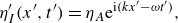 \begin{align} \eta '_I ( x', t' ) &= \eta _A \textrm{e}^{ \textrm{i}( k x' - \omega t' ) } , \\[9pt] \nonumber \end{align}
where amplitude $\phi _A$
and
$\phi _A$
and $\eta _A$
has the linear relation
$\eta _A$
has the linear relation
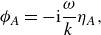 \begin{equation} \phi _A = - \textrm{i}\frac {\omega }{k} \eta _A, \end{equation}
satisfying the kinematic boundary condition (2.2c
), and $\omega$
and
$\omega$
and $k$
have the dispersion relation
$k$
have the dispersion relation
 \begin{equation} \omega ^2 = \frac { \sigma }{ \rho } k^3 + g k = \frac { \sigma }{ \rho } k^3 (1 + B), \end{equation}
satisfying the dynamic boundary conditions (2.2b ) and (2.2d ), where
 \begin{equation} B = \frac {\rho g}{\sigma k^2} \end{equation}
is the Bond number, characterising the relative effect between gravity and surface tension.
At large distances from the barrier, the surface elevation takes the far-field form:
 \begin{align} \eta ' & = \eta '_I + \eta '_R, \quad\quad \text{at } x' \rightarrow -\infty , \end{align}
 \begin{align} \eta ' & = \eta '_T, \qquad\qquad \text{at } x' \rightarrow +\infty , \\[9pt] \nonumber \end{align}
where
 \begin{align} \eta '_R & = R \eta '_I (-x', t') = R \eta _A \textrm{e}^{ \textrm{i}( - k x' - \omega t' ) } , \end{align}
 \begin{align} \eta '_T & = T \eta '_I (+x', t') = T \eta _A \textrm{e}^{ \textrm{i}( k x' - \omega t' ) } . \end{align}
Here, $T$
and
$T$
and $R$
are the complex transmission and reflection coefficients, respectively, which will be determined for their dependence on slip coefficient
$R$
are the complex transmission and reflection coefficients, respectively, which will be determined for their dependence on slip coefficient $\Lambda '$
, Bond number
$\Lambda '$
, Bond number $B$
, wavenumber
$B$
, wavenumber $k$
and barrier radius
$k$
and barrier radius $r'$
.
$r'$
.
For the linearised problem, where the incident wave (2.5) has the form of time harmonic oscillations $\textrm{e}^{-\textrm{i}\omega t'}$
and all governing equations including the dynamic contact line condition (2.4) are homogeneous, the wave fields
$\textrm{e}^{-\textrm{i}\omega t'}$
and all governing equations including the dynamic contact line condition (2.4) are homogeneous, the wave fields $\phi '$
and
$\phi '$
and $\eta '$
naturally adopt the same form of time harmonic oscillations:
$\eta '$
naturally adopt the same form of time harmonic oscillations:
 \begin{align} \phi ' ( x', y', t' ) &= \phi '(x', y') \textrm{e}^{ - \textrm{i}\omega t' } , \end{align}
 \begin{align} \eta ' ( x', t' ) &= \eta '(x') \textrm{e}^{ - \textrm{i}\omega t' } . \end{align}
The original spatiotemporal problem reduces to a purely spatial one for $\phi '(x', y')$
and
$\phi '(x', y')$
and $\eta '(x')$
.
$\eta '(x')$
.
The problem is transformed into a dimensionless form by introducing a new set of variables devoid of units:
 \begin{equation} t = \omega t',\quad (x, y, r) = k (x', y', r'),\quad \eta = \eta ' / \eta _A,\quad \phi = \phi ' / \phi _A,\quad p = p' / (\sigma k^2). \end{equation}
This rescaling simplifies the mathematical expressions and highlights the fundamental dynamics independent of specific scales of time and space. Furthermore, we redefine the slip coefficient $\Lambda '$
in dimensionless terms as
$\Lambda '$
in dimensionless terms as
 \begin{equation} \Lambda = \frac {\Lambda '}{c_p} = \frac {1}{\sqrt {1+B}} \sqrt {\frac {\rho }{\sigma k}} \Lambda ', \end{equation}
where $c_p = \omega /k = \sqrt {(1+B) \sigma k / \rho }$
is the phase speed of the capillary–gravity wave.
$c_p = \omega /k = \sqrt {(1+B) \sigma k / \rho }$
is the phase speed of the capillary–gravity wave.
The smallness conditions $k \eta _A \ll 1$
and
$k \eta _A \ll 1$
and $k \eta _A \ll r$
remain central to the dimensionless formulation. They ensure that the problem is governed by linearised dynamics, simplifying the analysis while maintaining accuracy for small perturbations.
$k \eta _A \ll r$
remain central to the dimensionless formulation. They ensure that the problem is governed by linearised dynamics, simplifying the analysis while maintaining accuracy for small perturbations.
The problem then reduces to solving two coupled BVPs for the velocity potential $\phi (x, y)$
and the surface elevation
$\phi (x, y)$
and the surface elevation $\eta (x)$
. For
$\eta (x)$
. For $\phi$
, following (2.2a
), (2.3) and (2.2c
), we solve:
$\phi$
, following (2.2a
), (2.3) and (2.2c
), we solve:
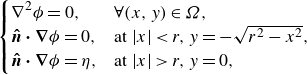 \begin{equation} \begin{cases} \displaystyle \nabla ^2 \phi = 0, & \forall (x, y) \in \Omega , \\ \displaystyle \boldsymbol{\hat {n} \cdot \nabla } \phi = 0, & \text{at } |x| \lt r, y = - \sqrt {r^2 - x^2}, \\ \displaystyle \boldsymbol{\hat {n} \cdot \nabla } \phi = \eta , & \text{at } |x| \gt r, y = 0, \end{cases} \end{equation}
where the domain $\Omega = \{(x, y) \in \mathbb{R}^2 \mid y \lt 0 \text{ and } x^2 + y^2 \gt r^2\}$
and
$\Omega = \{(x, y) \in \mathbb{R}^2 \mid y \lt 0 \text{ and } x^2 + y^2 \gt r^2\}$
and $\boldsymbol{\hat {n}}$
represents the outward normal vector of the domain boundary. For
$\boldsymbol{\hat {n}}$
represents the outward normal vector of the domain boundary. For $\eta$
, following (2.2b
), (2.2d
), (2.4) and (2.7), we solve, on the surface of the incident side (
$\eta$
, following (2.2b
), (2.2d
), (2.4) and (2.7), we solve, on the surface of the incident side ( $x \lt -r$
):
$x \lt -r$
):
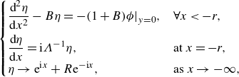 \begin{equation} \begin{cases} \displaystyle \frac {\textrm{d}^2 \eta }{\textrm{d}x^2} - B \eta = - (1+B) \phi \big |_{y=0}, & \forall x \lt -r, \\[8pt] \displaystyle \frac {\textrm{d} \eta }{\textrm{d}x} = \textrm{i}\Lambda ^{-1} \eta , & \text{at } x = -r, \\[3pt] \displaystyle \eta \rightarrow \textrm{e}^{\textrm{i}x} + R \textrm{e}^{-\textrm{i}x}, & \text{as } x \rightarrow -\infty , \end{cases} \end{equation}
and on the surface of the transmitted side ( $x \gt r$
):
$x \gt r$
):
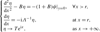 \begin{equation} \begin{cases} \displaystyle \frac {\textrm{d}^2 \eta }{\textrm{d}x^2} - B \eta = - (1+B) \phi \big |_{y=0}, & \forall x \gt r, \\[8pt] \displaystyle \frac {\textrm{d} \eta }{\textrm{d}x} = - \textrm{i}\Lambda ^{-1} \eta , & \text{at } x = r, \\[3pt] \displaystyle \eta \rightarrow T \textrm{e}^{ \textrm{i}x }, & \text{as } x \rightarrow +\infty . \end{cases} \end{equation}
Solving these BVPs allows us to determine the complex transmission ( $T$
) and reflection (
$T$
) and reflection ( $R$
) coefficients. These coefficients are dependent on three key dimensionless parameters: the Bond number
$R$
) coefficients. These coefficients are dependent on three key dimensionless parameters: the Bond number $B$
, the dimensionless radius of the barrier
$B$
, the dimensionless radius of the barrier $r$
and the dimensionless slip coefficient
$r$
and the dimensionless slip coefficient $\Lambda$
. This formulation highlights the interplay between fluid dynamics and the physical geometry of the barrier.
$\Lambda$
. This formulation highlights the interplay between fluid dynamics and the physical geometry of the barrier.
3. Solving boundary value problems
3.1. Expressing $\eta$
in terms of
$\phi$
$\eta$
in terms of
$\phi$


To solve the BVPs for $\eta$
, as specified in (2.12a
) and (2.12b
), we express
$\eta$
, as specified in (2.12a
) and (2.12b
), we express $\eta$
in terms of the boundary condition
$\eta$
in terms of the boundary condition $\phi |_{y=0} = \phi (x, 0)$
. These BVPs are modelled as inhomogeneous second-order linear differential equations (ISOLDEs), which are solved using the method of variation of constants (Hassani Reference Hassani2013). With detailed derivations provided in Appendix A, the solution for
$\phi |_{y=0} = \phi (x, 0)$
. These BVPs are modelled as inhomogeneous second-order linear differential equations (ISOLDEs), which are solved using the method of variation of constants (Hassani Reference Hassani2013). With detailed derivations provided in Appendix A, the solution for $\eta$
is given by
$\eta$
is given by
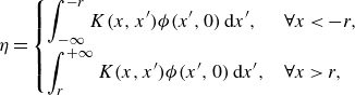 \begin{equation} \eta = \begin{cases} \displaystyle \int ^{- r}_{- \infty } K(x, x') \phi (x', 0) \: \textrm{d} x', & \forall x \lt -r, \\[8pt] \displaystyle \int ^{+ \infty }_{r} K(x, x') \phi (x', 0) \: \textrm{d} x', & \forall x \gt r, \end{cases} \end{equation}
where the dynamic kernel $K(x, x')$
is defined as
$K(x, x')$
is defined as
 \begin{equation} K(x, x') = \frac {1+B}{2\sqrt {B}} \left ( -\textrm{e}^{-2\textrm{i}\zeta } \textrm{e}^{\sqrt {B}(2r - |x + x'|)} + \textrm{e}^{-\sqrt {B}|x - x'|} \right ), \end{equation}
in which the parameter $\zeta$
is defined as
$\zeta$
is defined as
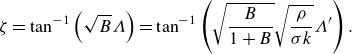 \begin{equation} \zeta = \tan ^{-1} \left ( \sqrt {B}\Lambda \right ) = \tan ^{-1} \left ( \sqrt {\frac {B}{1+B}} \sqrt {\frac {\rho }{\sigma k}} \Lambda ' \right ). \end{equation}
This formulation captures the spatial dependencies within the problem, allowing $\eta$
to be directly related to the boundary values of
$\eta$
to be directly related to the boundary values of $\phi$
.
$\phi$
.
The parameter $\zeta$
in (3.3) is introduced for mathematical convenience, simplifying the exponential expressions in the dynamic kernel
$\zeta$
in (3.3) is introduced for mathematical convenience, simplifying the exponential expressions in the dynamic kernel $K$
in (3.2). This parameter
$K$
in (3.2). This parameter $\zeta$
eventually encodes the dependence of the problem on the slip coefficient
$\zeta$
eventually encodes the dependence of the problem on the slip coefficient $\Lambda '$
. It ranges from
$\Lambda '$
. It ranges from $0$
to
$0$
to $\pi /2$
as the slip coefficient
$\pi /2$
as the slip coefficient $\Lambda '$
varies from
$\Lambda '$
varies from $0$
to
$0$
to $\infty$
, unless the Bond number
$\infty$
, unless the Bond number $B = 0$
. From now on,
$B = 0$
. From now on, $\zeta$
replaces
$\zeta$
replaces $\Lambda$
to act as the dimensionless slip parameter in the dynamic contact line conditions. It is worth pointing out that, with the inverse trigonometric function arctangent in (3.3), this slip parameter
$\Lambda$
to act as the dimensionless slip parameter in the dynamic contact line conditions. It is worth pointing out that, with the inverse trigonometric function arctangent in (3.3), this slip parameter $\zeta$
may be interpreted as an ‘angle’. However, it should not be confused with the contact angle at the edges, whose deviation from the static contact angle is given by
$\zeta$
may be interpreted as an ‘angle’. However, it should not be confused with the contact angle at the edges, whose deviation from the static contact angle is given by $\tan ^{-1} (\partial _{x'}\eta ')$
.
$\tan ^{-1} (\partial _{x'}\eta ')$
.
3.2. Expressing
$\phi$
in terms of
$\eta$


3.2.1. Conformal mapping
In addressing the BVP for $\phi (x, y)$
as defined in (2.11), we employ a conformal mapping technique. This method transforms the liquid domain
$\phi (x, y)$
as defined in (2.11), we employ a conformal mapping technique. This method transforms the liquid domain $\Omega$
into the lower half-space
$\Omega$
into the lower half-space $H = \{(u, v) \in \mathbb{R}^2 \mid v \lt 0\}$
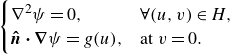
. Specifically, the free surface and the lower half of the cylindrical barrier surface are mapped onto the real axis, as depicted in figure 2. Defining
$H = \{(u, v) \in \mathbb{R}^2 \mid v \lt 0\}$
. Specifically, the free surface and the lower half of the cylindrical barrier surface are mapped onto the real axis, as depicted in figure 2. Defining $z = x + \textrm{i} y$
and
$z = x + \textrm{i} y$
and $w = u + \textrm{i} v$
, the mapping from the
$w = u + \textrm{i} v$
, the mapping from the $z$
-plane to the
$z$
-plane to the $w$
-plane is prescribed by
$w$
-plane is prescribed by
 \begin{equation} w = \frac {z}{r} + \frac {r}{z}, \end{equation}
or, in component form,
 \begin{equation} u = \frac {(x^2 + y^2 + r^2) x}{(x^2 + y^2) r}, \quad v = \frac {(x^2 + y^2 - r^2) y}{(x^2 + y^2) r}. \end{equation}
This conformal mapping, known as the Joukowsky transform and historically used for applications like aerofoil design (Joukowsky Reference Joukowsky1910), is extended here to analyse capillary–gravity wave scattering.
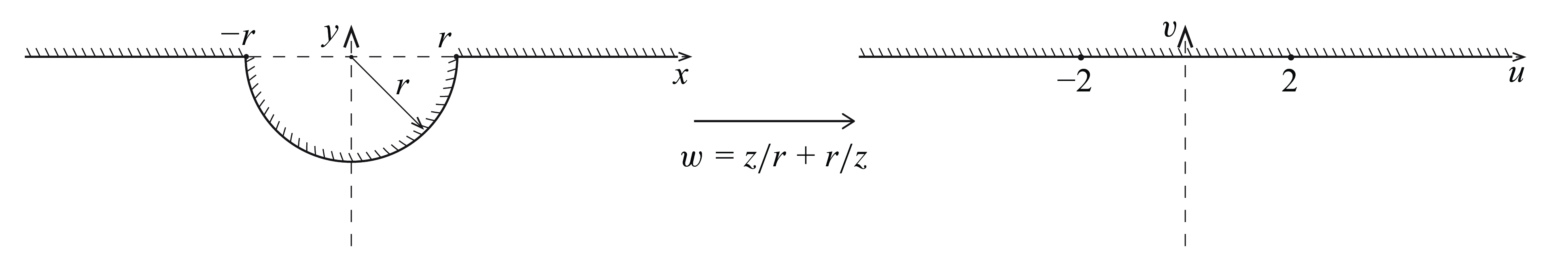
Figure 2. Schematic for the conformal mapping.
In this transformed coordinate system, the free surface is defined by $v = 0, |u| \gt 2$
and the barrier surface by
$v = 0, |u| \gt 2$
and the barrier surface by $v = 0, |u| \lt 2$
. The transformation preserves the Laplace equation; thus, the transformed BVP for
$v = 0, |u| \lt 2$
. The transformation preserves the Laplace equation; thus, the transformed BVP for $\psi$
, related to
$\psi$
, related to $\phi$
by
$\phi$
by $\psi (u, v) = \phi (x, y)$
, is expressed as
$\psi (u, v) = \phi (x, y)$
, is expressed as
 \begin{equation} \begin{cases} \displaystyle \nabla ^2 \psi = 0, & \forall (u, v) \in H, \\ \displaystyle \boldsymbol{\hat {n} \cdot \nabla } \psi = g(u), & \text{at } v = 0. \end{cases} \end{equation}
The boundary function $g(u)$
is defined by
$g(u)$
is defined by
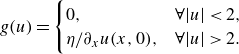 \begin{equation} g(u) = \begin{cases} \displaystyle 0, & \forall |u| \lt 2, \\ \displaystyle \eta / \partial _x u(x, 0), & \forall |u| \gt 2. \end{cases} \end{equation}
3.2.2. Fourier transform
Under normal circumstances, the BVP for $\psi (u, v)$
as outlined in (3.6), being a Laplace equation with Neumann boundary conditions in the lower half-space, should be solvable using the Green’s function approach. However, our situation presents a unique challenge due to the behaviour of the field at infinity (
$\psi (u, v)$
as outlined in (3.6), being a Laplace equation with Neumann boundary conditions in the lower half-space, should be solvable using the Green’s function approach. However, our situation presents a unique challenge due to the behaviour of the field at infinity ( $u \to \pm \infty$
), where it does not vanish. This non-vanishing at infinity is mirrored by the corresponding Green’s function for the Neumann boundary condition in the lower half-space, which similarly does not vanish as
$u \to \pm \infty$
), where it does not vanish. This non-vanishing at infinity is mirrored by the corresponding Green’s function for the Neumann boundary condition in the lower half-space, which similarly does not vanish as $u \to \pm \infty$
. Consequently, the integral involving the Green’s function multiplied by
$u \to \pm \infty$
. Consequently, the integral involving the Green’s function multiplied by $\nabla \psi$
at infinity does not converge, rendering this approach infeasible.
$\nabla \psi$
at infinity does not converge, rendering this approach infeasible.
We opted for a different approach, using the Fourier transform method. This elegant technique circumvents the difficulties associated with the traditional Green’s function method and provides a robust solution to the problem.
We apply the following Fourier transform to (3.6):
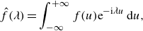 \begin{equation} \hat {f}(\lambda ) = \int _{-\infty }^{+\infty } f(u) \textrm{e}^{-\textrm{i}\lambda u} \: \textrm{d} u, \end{equation}
we obtain
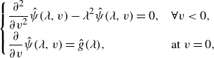 \begin{equation} \begin{cases} \displaystyle \frac {\partial ^2}{\partial v^2} \hat {\psi }(\lambda , v) - \lambda ^2 \hat {\psi }(\lambda , v) = 0, & \forall v \lt 0, \\[6pt] \displaystyle \frac {\partial }{\partial v} \hat {\psi }(\lambda , v) = \hat {g}(\lambda ), & \text{at } v = 0, \end{cases} \end{equation}
where $\hat {\psi }$
and
$\hat {\psi }$
and $\hat {g}$
are the Fourier transform of
$\hat {g}$
are the Fourier transform of $\psi$
and
$\psi$
and $g$
. This simplifies the problem to a homogeneous ordinary differential equation (ODE) with respect to
$g$
. This simplifies the problem to a homogeneous ordinary differential equation (ODE) with respect to $v$
, allowing
$v$
, allowing $\hat {\psi }(\lambda , v)$
to be expressed as
$\hat {\psi }(\lambda , v)$
to be expressed as
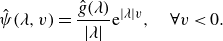 \begin{equation} \hat {\psi }(\lambda , v) = \frac {\hat {g}(\lambda )}{|\lambda |} \textrm{e}^{|\lambda | v}, \quad \forall v \lt 0. \end{equation}
An inverse Fourier transform yields the solution to (3.6):
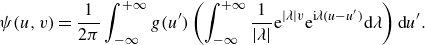 \begin{align} \psi (u, v) &= \frac {1}{2\pi } \int _{-\infty }^{+\infty } g(u') \left ( \int _{-\infty }^{+\infty } \frac {1}{|\lambda |} \textrm{e}^{|\lambda | v} \textrm{e}^{\textrm{i}\lambda (u - u')} \textrm{d} \lambda \right ) \textrm{d} u' . \end{align}
By evaluating at $v = 0$
, with detailed derivations provided in Appendix B, we derive the expression for
$v = 0$
, with detailed derivations provided in Appendix B, we derive the expression for $\phi (x,0) = \psi (u,0)$
, giving
$\phi (x,0) = \psi (u,0)$
, giving
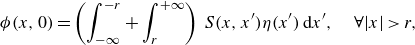 \begin{align} \phi (x, 0) &= \left ( \int _{-\infty }^{-r} + \int _{r}^{+\infty } \right ) \, S (x, x') \eta (x') \: \textrm{d} x' , \quad \forall |x| \gt r, \end{align}
where the geometric kernel $S(x, x')$
is defined as
$S(x, x')$
is defined as
 \begin{equation} S (x, x') = - \pi ^{-1} \left ( \ln { \left | \frac {x}{r} + \frac {r}{x} - \frac {x'}{r} - \frac {r}{x'} \right | } + \gamma \right ), \end{equation}
where $\gamma$
is the Euler–Mascheroni constant (
$\gamma$
is the Euler–Mascheroni constant ( $= 0.57722 \cdots$
).
$= 0.57722 \cdots$
).
We have now solved the BVPs referred to in (2.11)–(2.12b
). Specifically, the solutions for $\eta$
in terms of
$\eta$
in terms of $\phi (x, 0)$
are presented in (3.1), while the solution for
$\phi (x, 0)$
are presented in (3.1), while the solution for $\phi (x, 0)$
in terms of
$\phi (x, 0)$
in terms of $\eta$
is provided in (3.12). By combining (3.1) and (3.12), we can derive a single integral equation for
$\eta$
is provided in (3.12). By combining (3.1) and (3.12), we can derive a single integral equation for $\phi (x, 0)$
. Solving this integral equation will allow us to determine the complex transmission (
$\phi (x, 0)$
. Solving this integral equation will allow us to determine the complex transmission ( $T$
) and reflection (
$T$
) and reflection ( $R$
) coefficients.
$R$
) coefficients.
4. Solving integral equations
Let us denote $f(x) = \phi (x, 0)$
for simplicity. By combining (3.1) and (3.12), we arrive at the following integral equation for
$f(x) = \phi (x, 0)$
for simplicity. By combining (3.1) and (3.12), we arrive at the following integral equation for $f(x)$
, which must also satisfy specific far-field forms as
$f(x)$
, which must also satisfy specific far-field forms as $x \to \pm \infty$
:
$x \to \pm \infty$
:
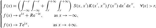 \begin{equation} \begin{cases} \displaystyle f(x) = \left ( \int _{-\infty }^{-r} \int _{-\infty }^{-r} + \int _{r}^{+\infty } \int _{r}^{+\infty } \right ) \, S (x, x') K(x', x'') f(x'') \: \textrm{d} x' \: \textrm{d} x'' , \quad \forall |x| \gt r, \\[8pt] \displaystyle f(x) \rightarrow \textrm{e}^{\textrm{i}x} + R \textrm{e}^{-\textrm{i}x}, \qquad \ \text{as } x \rightarrow -\infty , \\[8pt] \displaystyle f(x) \rightarrow T \textrm{e}^{\textrm{i}x}, \quad \qquad \qquad \text{as } x \rightarrow +\infty . \end{cases} \end{equation}
4.1. Even-odd separation
To solve this problem, we consider two cases where $f$
is either an even or odd function of
$f$
is either an even or odd function of $x$
. Denoting these as
$x$
. Denoting these as $f_e$
and
$f_e$
and $f_o$
respectively, we can express
$f_o$
respectively, we can express $f$
as
$f$
as $f = f_e + f_o$
. The equations for the even solution
$f = f_e + f_o$
. The equations for the even solution $f_e$
and the odd solution
$f_e$
and the odd solution $f_o$
then become
$f_o$
then become
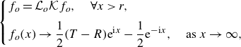
 \begin{align} &\begin{cases} \displaystyle f_e(x) = \int _{r}^{+ \infty } L_e(x, x') \left (\int ^{+ \infty }_{r} K(x', x'') f_e(x'') {\textrm d}x''\right ) \textrm{d}x' , \quad \ \forall x \gt r, \\[9pt] \displaystyle f_e(x) \rightarrow \frac {1}{2} (T+R) \textrm{e}^{\textrm{i}x} + \frac {1}{2} \textrm{e}^{-\textrm{i}x} , \quad \ \text{as } x \rightarrow \infty , \end{cases} \end{align}
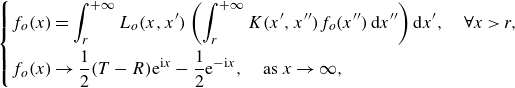 \begin{align} &\begin{cases} \displaystyle f_o(x) = \int _{r}^{+ \infty } L_o(x, x') \left (\int ^{+ \infty }_{r} K(x', x'') f_o(x'') \: \textrm{d} x''\right ) \textrm{d} x' , \quad \forall x \gt r, \\[9pt] \displaystyle f_o(x) \rightarrow \frac {1}{2} (T-R) \textrm{e}^{\textrm{i}x} - \frac {1}{2} \textrm{e}^{-\textrm{i}x} , \quad \text{as } x \rightarrow \infty , \end{cases} \end{align}
where dynamic kernel $K$
is defined in (3.2), and geometric kernel
$K$
is defined in (3.2), and geometric kernel $L_e$
,
$L_e$
, $L_o$
are defined by
$L_o$
are defined by $S$
, given in (3.13):
$S$
, given in (3.13):
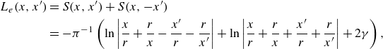 \begin{align} L_e(x,x') &= S (x, x') + S (x, -x') \nonumber \\ &= - \pi ^{-1} \left ( \ln \left | \frac {x}{r} + \frac {r}{x} - \frac {x'}{r} - \frac {r}{x'} \right | + \ln \left | \frac {x}{r} + \frac {r}{x} + \frac {x'}{r} + \frac {r}{x'} \right | + 2 \gamma \right ) , \end{align}
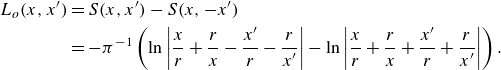 \begin{align} L_o(x,x') &= S (x, x') - S (x, -x') \nonumber \\ &= - \pi ^{-1} \left ( \ln \left | \frac {x}{r} + \frac {r}{x} - \frac {x'}{r} - \frac {r}{x'} \right | - \ln \left | \frac {x}{r} + \frac {r}{x} + \frac {x'}{r} + \frac {r}{x'} \right | \right ) . \end{align}
In the abstract operator language, (4.2a ) can be written as
 \begin{equation} \begin{cases} \displaystyle f_e = \mathcal{L}_e \mathcal{K} f_e, \quad \forall x \gt r, \\[5pt] \displaystyle f_e(x) \rightarrow \frac {1}{2} (T+R) \textrm{e}^{\textrm{i}x} + \frac {1}{2} \textrm{e}^{-\textrm{i}x} , \quad \text{as } x \rightarrow \infty , \end{cases} \end{equation}
where $\mathcal{L}_e$
and
$\mathcal{L}_e$
and $\mathcal{K}$
are the integral operators integrate from
$\mathcal{K}$
are the integral operators integrate from $r$
to
$r$
to $\infty$
with even geometric kernel
$\infty$
with even geometric kernel $L_e$
given in (4.3) and dynamic kernel
$L_e$
given in (4.3) and dynamic kernel $K$
given in (3.2). Then, (4.2b
) can be written as
$K$
given in (3.2). Then, (4.2b
) can be written as
 \begin{equation} \begin{cases} \displaystyle f_o = \mathcal{L}_o \mathcal{K} f_o, \quad \forall x \gt r, \\[5pt] \displaystyle f_o(x) \rightarrow \frac {1}{2} (T-R) \textrm{e}^{\textrm{i}x} - \frac {1}{2} \textrm{e}^{-\textrm{i}x} , \quad \text{as } x \rightarrow \infty , \end{cases} \end{equation}
where $\mathcal{L}_o$
is the integral operator with odd geometric kernel
$\mathcal{L}_o$
is the integral operator with odd geometric kernel $L_o$
given in (4.3).
$L_o$
given in (4.3).
4.2. Deviation from far-field behaviour
If we define $f_e$
and
$f_e$
and $f_o$
in terms of their deviations from far fields by
$f_o$
in terms of their deviations from far fields by $h_e(x)$
and
$h_e(x)$
and $h_o(x)$
:
$h_o(x)$
:
 \begin{align} f_e &= \frac {1}{2} (T+R) \textrm{e}^{\textrm{i}x} + \frac {1}{2} \textrm{e}^{-\textrm{i}x} + h_e(x), \\[-12pt] \nonumber \end{align}
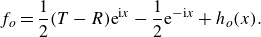 \begin{align} f_o &= \frac {1}{2} (T-R) \textrm{e}^{\textrm{i}x} - \frac {1}{2} \textrm{e}^{-\textrm{i}x} + h_o(x). \end{align}
We then derive equations for the near fields $h_e$
and
$h_e$
and $h_o$
:
$h_o$
:
 \begin{align} &\begin{cases} \displaystyle h_e = \mathcal{L}_e \mathcal{K} h_e + \frac {1}{2} (T+R) (\mathcal{L}_e \mathcal{K} - \mathcal{I}) \textrm{e}^{\textrm{i}x} + \frac {1}{2} (\mathcal{L}_e \mathcal{K} - \mathcal{I}) \textrm{e}^{-\textrm{i}x} , \quad \forall x \gt r, \\[8pt] \displaystyle h_e(x) \rightarrow 0 , \quad \text{as } x \rightarrow \infty , \end{cases} \end{align}
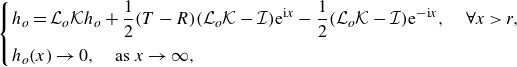 \begin{align} &\begin{cases} \displaystyle h_o = \mathcal{L}_o \mathcal{K} h_o + \frac {1}{2} (T-R) (\mathcal{L}_o \mathcal{K} - \mathcal{I}) \textrm{e}^{\textrm{i}x} - \frac {1}{2} (\mathcal{L}_o \mathcal{K} - \mathcal{I}) \textrm{e}^{-\textrm{i}x} , \quad \forall x \gt r, \\[8pt] \displaystyle h_o(x) \rightarrow 0 , \quad \text{as } x \rightarrow \infty , \end{cases} \end{align}
where $\mathcal{I}$
is the identity operator, which takes a function to the same function. Based on the symmetry of (4.7), we seek solutions of
$\mathcal{I}$
is the identity operator, which takes a function to the same function. Based on the symmetry of (4.7), we seek solutions of $h_e$
and
$h_e$
and $h_o$
in the form:
$h_o$
in the form:
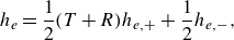 \begin{align} h_e &= \frac {1}{2} (T+R) h_{e, +} + \frac {1}{2} h_{e, -}, \end{align}
 \begin{align} h_o &= \frac {1}{2} (T-R) h_{o, +} - \frac {1}{2} h_{o, -}, \end{align}
where $h_{e, \pm }$
and
$h_{e, \pm }$
and $h_{o, \pm }$
are to be determined. Substituting (4.8) into (4.7) yields
$h_{o, \pm }$
are to be determined. Substituting (4.8) into (4.7) yields
 \begin{align} (T + R) \{ h_{e,+} - \mathcal{L}_e \mathcal{K} h_{e,+} - (\mathcal{L}_e \mathcal{K} - \mathcal{I}) \textrm{e}^{\textrm{i}x} \} &= - \{ h_{e,-} - \mathcal{L}_e \mathcal{K} h_{e,-} - (\mathcal{L}_e \mathcal{K} - \mathcal{I}) \textrm{e}^{- \textrm{i}x} \} , \end{align}
 \begin{align} (T - R) \{ h_{o,+} - \mathcal{L}_o \mathcal{K} h_{o,+} - (\mathcal{L}_o \mathcal{K} - \mathcal{I}) \textrm{e}^{\textrm{i}x} \} &= \{ h_{o,-} - \mathcal{L}_o \mathcal{K} h_{o,-} - (\mathcal{L}_o \mathcal{K} - \mathcal{I}) \textrm{e}^{- \textrm{i}x} \} . \end{align}
A possible solution for $h_{e, \pm }$
and
$h_{e, \pm }$
and $h_{o, \pm }$
that satisfies (4.9) would be letting both sides equal to
$h_{o, \pm }$
that satisfies (4.9) would be letting both sides equal to $0$
:
$0$
:
 \begin{equation} h_{\chi , \pm } = \mathcal{L}_{\chi } \mathcal{K} h_{\chi ,\pm } + (\mathcal{L}_{\chi } \mathcal{K} - \mathcal{I}) \textrm{e}^{\pm \textrm{i}x} , \end{equation}
where $\chi$
takes the values ‘
$\chi$
takes the values ‘ $e$
’ for even and ‘
$e$
’ for even and ‘ $o$
’ for odd. Then,
$o$
’ for odd. Then, $(\mathcal{L}_{\chi } \mathcal{K} - \mathcal{I}) \textrm{e}^{\pm \textrm{i}x}$
can be calculated analytically:
$(\mathcal{L}_{\chi } \mathcal{K} - \mathcal{I}) \textrm{e}^{\pm \textrm{i}x}$
can be calculated analytically:
 \begin{align}& (\mathcal{L}_{\chi } \mathcal{K} - \mathcal{I}) \textrm{e}^{\pm \textrm{i}x} =\int _{r}^{+ \infty } L_{\chi }(x, x') \left ( \int _{r}^{+ \infty } K(x', x'') \textrm{e}^{\pm \textrm{i}x''} \: \textrm{d} x'' \right ) \textrm{d} x' - \textrm{e}^{\pm \textrm{i}x} , \end{align}
 \begin{align} &\,\,= - \textrm{e}^{\pm \textrm{i}x} + \frac {1}{2 \sqrt {B}} \left [ - (\sqrt {B} \pm \textrm{i}) \textrm{e}^{-2\textrm{i}\zeta } + (-\sqrt {B} \pm \textrm{i}) \right ] \textrm{e}^{(\sqrt {B} \pm \textrm{i}) r} I_{1, \chi } + I_{2, \chi , \pm } , \\[6pt] \nonumber \end{align}
where the expressions for $I_1$
and
$I_1$
and $I_2$
are given in Appendix C.
$I_2$
are given in Appendix C.
4.3. Calculating
$T$
and
$R$


Finally, to ensure that the near fields $h_e$
and
$h_e$
and $h_o$
given in (4.7) approach to
$h_o$
given in (4.7) approach to $0$
as
$0$
as $x \rightarrow \infty$
, we have
$x \rightarrow \infty$
, we have
 \begin{align} \frac {1}{2} (T+R) h_{e, +} + \frac {1}{2} h_{e, -} &\rightarrow 0, \quad \text{as } x \rightarrow \infty , \end{align}
 \begin{align} \frac {1}{2} (T-R) h_{o, +} - \frac {1}{2} h_{o, -} &\rightarrow 0, \quad \text{as } x \rightarrow \infty , \end{align}
from which we can infer the coefficients $T$
and
$T$
and $R$
:
$R$
:
 \begin{align} T &= - \frac {1}{2} \left ( C_e - C_o \right ) , \end{align}
 \begin{align} R &= - \frac {1}{2} \left ( C_e + C_o \right ) , \end{align}
where
 \begin{equation} C_e = \lim _{x \rightarrow \infty } \frac {h_{e, -}}{h_{e, +}}, \qquad C_o = \lim _{x \rightarrow \infty } \frac {h_{o, -}}{h_{o, +}} . \end{equation}
Therefore, we have reduced the integral equation problem for $f(x) = \phi (x, 0)$
given in (4.1) to solve the simpler integral equations in (4.10), and substitute into (4.14) to obtain the transmission coefficient
$f(x) = \phi (x, 0)$
given in (4.1) to solve the simpler integral equations in (4.10), and substitute into (4.14) to obtain the transmission coefficient $T$
and reflection coefficient
$T$
and reflection coefficient $R$
. This approach guarantees that the solutions converge to the desired far-field behaviour, ensuring the physical relevance and mathematical consistency of the results.
$R$
. This approach guarantees that the solutions converge to the desired far-field behaviour, ensuring the physical relevance and mathematical consistency of the results.
4.4. Nyström method: numerically solving integral equations
The integral equations in (4.10) share the same form of
 \begin{equation} h = \mathcal{L} \mathcal{K} h + g, \end{equation}
which can be effectively solved numerically using the Nyström method. This approach discretises the integral operators $\mathcal{L}$
and
$\mathcal{L}$
and $\mathcal{K}$
into matrices, transforming the integral equations into matrix equations. Specifically, the discretisation is defined as
$\mathcal{K}$
into matrices, transforming the integral equations into matrix equations. Specifically, the discretisation is defined as
 \begin{equation} \boldsymbol{h}_i = h(x_i), \quad \boldsymbol{g}_i = g(x_i), \quad \unicode{x1D647}_{\chi , ij} = L_\chi (x_i, x_j) \Delta x, \quad \unicode{x1D646}_{ij} = K(x_i, x_j) \Delta x, \end{equation}
where $x_i = r + i\Delta x$
, the step size
$x_i = r + i\Delta x$
, the step size $\Delta x = l / N$
and the integral range
$\Delta x = l / N$
and the integral range $l$
is truncated to ten times the wavelength,
$l$
is truncated to ten times the wavelength, $20\pi$
. The number of representative points,
$20\pi$
. The number of representative points, $N$
, is selected as 2000 to ensure sufficient accuracy.
$N$
, is selected as 2000 to ensure sufficient accuracy.
A convergence test was performed by halving and doubling $N$
for the relevant ranges of Bond number
$N$
for the relevant ranges of Bond number $B$
(
$B$
( $0.01 \leqslant B \leqslant 100$
) and dimensionless radius
$0.01 \leqslant B \leqslant 100$
) and dimensionless radius $r$
(
$r$
( $0.01 \leqslant r \leqslant 10$
), together with the range of slip parameter
$0.01 \leqslant r \leqslant 10$
), together with the range of slip parameter $\zeta$
(
$\zeta$
( $0 \leqslant \zeta \leqslant \pi /2$
). Among the tested combinations, the largest discrepancy of the calculated
$0 \leqslant \zeta \leqslant \pi /2$
). Among the tested combinations, the largest discrepancy of the calculated $T$
and
$T$
and $R$
arose at small values of
$R$
arose at small values of $B=0.01$
and
$B=0.01$
and $r=0.01$
, while
$r=0.01$
, while $\zeta$
has a negligible influence on the overall error. The largest difference of the calculated
$\zeta$
has a negligible influence on the overall error. The largest difference of the calculated $|T|$
between
$|T|$
between $N=1000$
and
$N=1000$
and $N=2000$
reached approximately
$N=2000$
reached approximately $3.6\,\%$
. Increasing to
$3.6\,\%$
. Increasing to $N=4000$
reduced the discrepancy of the calculated
$N=4000$
reduced the discrepancy of the calculated $|T|$
to approximately
$|T|$
to approximately $0.8\,\%$
. These results confirm that
$0.8\,\%$
. These results confirm that $N=2000$
is sufficiently accurate even under the most challenging scenario.
$N=2000$
is sufficiently accurate even under the most challenging scenario.
Special attention is given to the diagonal elements of $\unicode{x1D647}_{\chi , ij}$
due to the weak singularity at
$\unicode{x1D647}_{\chi , ij}$
due to the weak singularity at $x = x'$
, arising from the logarithmic term
$x = x'$
, arising from the logarithmic term $\ln | x/r + r/x - x'/r - r/x' |$
. To address this, the singularity is mitigated using the following approximation:
$\ln | x/r + r/x - x'/r - r/x' |$
. To address this, the singularity is mitigated using the following approximation:
 \begin{equation} \int _{x_i}^{x_i+\Delta x} \ln \left | \frac {x}{r} + \frac {r}{x} - \frac {x_i}{r} - \frac {r}{x_i} \right | \: \textrm{d} x \approx \ln \left ( \left ( \frac {1}{r} - \frac {r}{x_i^2} \right ) \Delta x \right ) - 1. \end{equation}
This procedure allows the integral equation (4.15) to be converted into the matrix equation:
 \begin{equation} \boldsymbol{h} = \unicode{x1D647}\unicode{x1D646} \boldsymbol{h} + \boldsymbol{g}, \end{equation}
which can be solved explicitly as
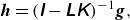 \begin{equation} \boldsymbol{h} = ( \unicode{x1D644} - \unicode{x1D647} \unicode{x1D646} )^{-1} \boldsymbol{g}, \end{equation}
where $\unicode{x1D644}$
denotes the identity matrix.
$\unicode{x1D644}$
denotes the identity matrix.
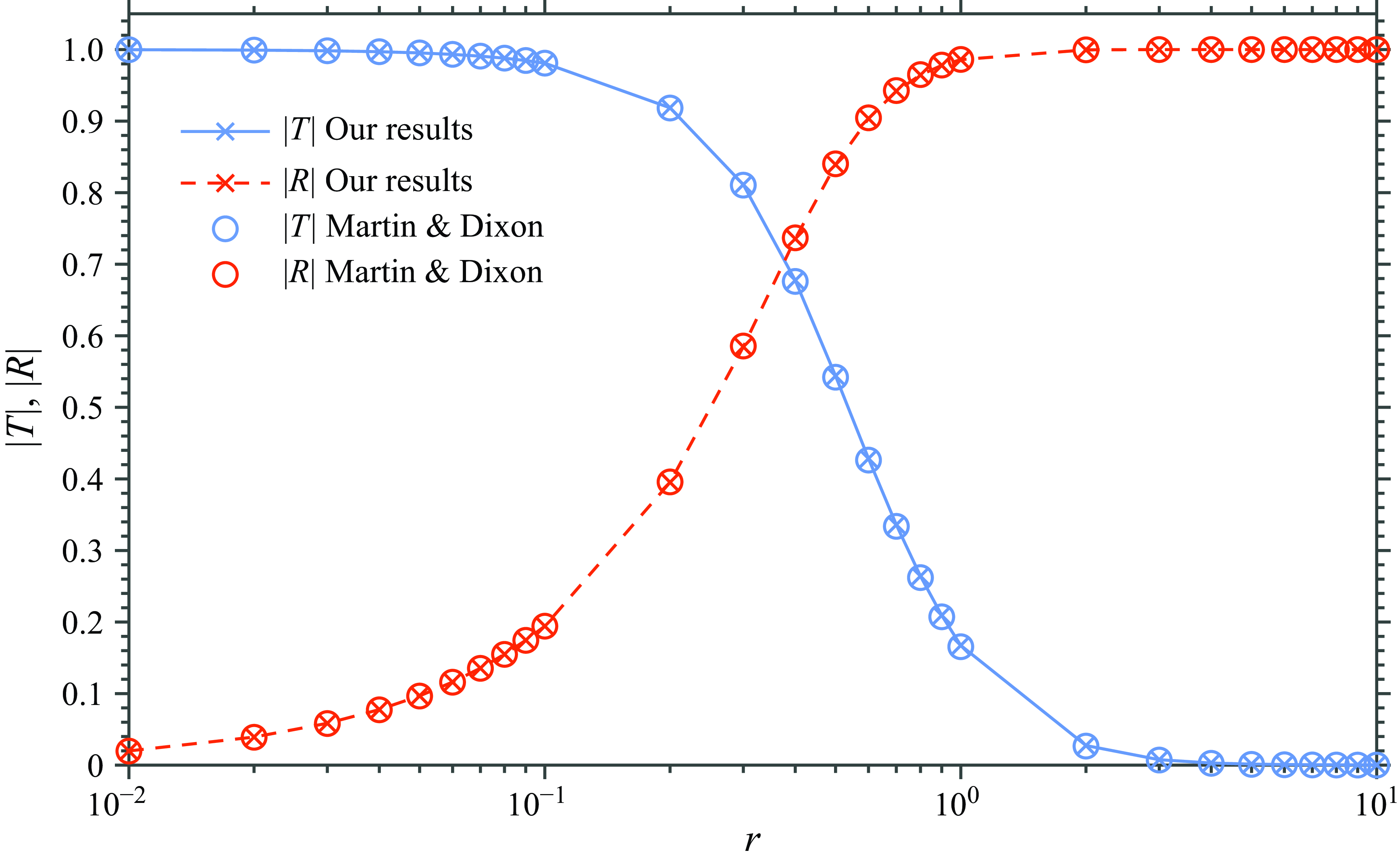
Figure 3. Comparison of results for gravity wave scattering between our semi-analytical results and results from Martin & Dixon (Reference Martin and Dixon1983) for the transmission $|T|$
and reflection
$|T|$
and reflection $|R|$
as a function of the dimensionless barrier radius
$|R|$
as a function of the dimensionless barrier radius $r$
(the dimensional radius
$r$
(the dimensional radius $r'$
multiplied by the wavenumber
$r'$
multiplied by the wavenumber $k$
).
$k$
).
5. Gravity waves: comparison with previous work
For pure gravity waves ( $B = \infty$
), the second-order derivative term
$B = \infty$
), the second-order derivative term ${\textrm d}^2 \eta / {\textrm d}x^2$
in (2.12) becomes negligible. As a result, the BVPs for
${\textrm d}^2 \eta / {\textrm d}x^2$
in (2.12) becomes negligible. As a result, the BVPs for $\eta$
specified in these equations become self-contained solutions:
$\eta$
specified in these equations become self-contained solutions:
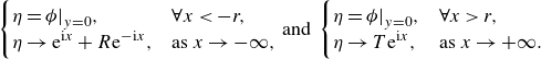 \begin{equation} \begin{cases} \displaystyle \eta = \phi \big |_{y=0}, & \forall x \lt -r, \\ \displaystyle \eta \rightarrow \textrm{e}^{\textrm{i}x} + R \textrm{e}^{-\textrm{i}x}, & \text{as } x \rightarrow -\infty , \end{cases} \text{and } \begin{cases} \displaystyle \eta = \phi \big |_{y=0}, & \forall x \gt r, \\ \displaystyle \eta \rightarrow T \textrm{e}^{ \textrm{i}x }, & \text{as } x \rightarrow +\infty . \end{cases} \end{equation}
In conjunction with the solution to (2.11) provided in (3.12), we formulate the integral equation problem for $f(x) = \phi (x, 0)$
:
$f(x) = \phi (x, 0)$
:
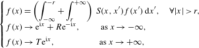 \begin{equation} \begin{cases} \displaystyle f(x) = \left ( \int _{-\infty }^{-r} + \int _{r}^{+\infty } \right ) \, S (x, x') f(x') \: \textrm{d} x' , \quad \forall |x| \gt r, \\[6pt] \displaystyle f(x) \rightarrow \textrm{e}^{\textrm{i}x} + R \textrm{e}^{-\textrm{i}x}, \qquad \ \text{as } x \rightarrow -\infty , \\[4pt] \displaystyle f(x) \rightarrow T \textrm{e}^{\textrm{i}x}, \quad \qquad \qquad \text{as } x \rightarrow +\infty , \end{cases} \end{equation}
where $S$
is defined in (3.13). Following the analyses in §§ 4.1 and 4.2, we derive the equations for
$S$
is defined in (3.13). Following the analyses in §§ 4.1 and 4.2, we derive the equations for $h_{\chi , \pm }$
(where
$h_{\chi , \pm }$
(where $\chi$
represents either even
$\chi$
represents either even $h_{e, \pm }$
or odd
$h_{e, \pm }$
or odd $h_{o, \pm }$
solutions):
$h_{o, \pm }$
solutions):
 \begin{equation} h_{\chi , \pm } = \mathcal{L}_{\chi } h_{\chi ,\pm } + (\mathcal{L}_{\chi } - \mathcal{I}) \textrm{e}^{\pm \textrm{i}x} , \end{equation}
where $\mathcal{L}_{\chi }$
(either
$\mathcal{L}_{\chi }$
(either $\mathcal{L}_{e}$
or
$\mathcal{L}_{e}$
or $\mathcal{L}_{o}$
) shares the kernel definition detailed in (4.3). Equation (5.3) requires numerical resolution, typically using the method outlined in § 4.4. The resulting solutions
$\mathcal{L}_{o}$
) shares the kernel definition detailed in (4.3). Equation (5.3) requires numerical resolution, typically using the method outlined in § 4.4. The resulting solutions $h_{e, \pm }$
and
$h_{e, \pm }$
and $h_{o, \pm }$
are then used to compute the transmission
$h_{o, \pm }$
are then used to compute the transmission $T$
and reflection
$T$
and reflection $R$
coefficients, as defined in (4.14). The term
$R$
coefficients, as defined in (4.14). The term $(\mathcal{L}_{\chi } - \mathcal{I}) \textrm{e}^{\pm \textrm{i}x}$
can be expressed analytically as
$(\mathcal{L}_{\chi } - \mathcal{I}) \textrm{e}^{\pm \textrm{i}x}$
can be expressed analytically as
 \begin{equation} (\mathcal{L}_{\chi } - \mathcal{I}) \textrm{e}^{\pm \textrm{i}x} = I_{2, \chi , \pm } - \textrm{e}^{\pm \textrm{i}x} , \end{equation}
where $I_2$
is evaluated in Appendix C. The semi-analytical results are compared with the multipole method results from Martin & Dixon (Reference Martin and Dixon1983) in figure 3 and table 3 in Appendix F, demonstrating their agreement on the reduction of transmission as the barrier size increases.
$I_2$
is evaluated in Appendix C. The semi-analytical results are compared with the multipole method results from Martin & Dixon (Reference Martin and Dixon1983) in figure 3 and table 3 in Appendix F, demonstrating their agreement on the reduction of transmission as the barrier size increases.
6. Capillary–gravity waves: phase difference and energy conservation at contact line limits
In this section, we analyse the phase difference between the transmission and reflection coefficients, as well as the energy conservation of wave fields in two limiting cases of the contact line conditions: the fixed contact line ( $\Lambda ' = 0$
) and the free contact line (
$\Lambda ' = 0$
) and the free contact line ( $\Lambda ' = \pi /2$
).
$\Lambda ' = \pi /2$
).
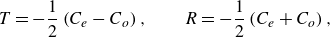 \begin{equation} T = - \frac {1}{2} \left ( C_e - C_o \right ) , \qquad R = - \frac {1}{2} \left ( C_e + C_o \right ) , \end{equation}
where $C_\chi$
(
$C_\chi$
( $\chi$
takes the values ‘
$\chi$
takes the values ‘ $e$
’ for even and ‘
$e$
’ for even and ‘ $o$
’ for odd) is given in (4.14c
) as
$o$
’ for odd) is given in (4.14c
) as
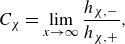 \begin{equation} C_\chi = \lim _{x \rightarrow \infty } \frac {h_{\chi , -}}{h_{\chi , +}}, \end{equation}
and $h_{\chi , \pm }$
satisfies (4.10):
$h_{\chi , \pm }$
satisfies (4.10):
 \begin{equation} h_{\chi , \pm } = \mathcal{L}_{\chi } \mathcal{K} h_{\chi ,\pm } + (\mathcal{L}_{\chi } \mathcal{K} - \mathcal{I}) \textrm{e}^{\pm \textrm{i}x}, \end{equation}
with the dynamic kernel $K$
given in (3.2) and (3.3).
$K$
given in (3.2) and (3.3).
For the two limiting cases of contact lines, the dynamic kernel $K$
in (3.2) and (3.3) reduces to
$K$
in (3.2) and (3.3) reduces to
 \begin{align} &\text{Fixed contact lines}\,(\Lambda = 0): &K(x,x') &= \frac {1+B}{2\sqrt {B}} \left ( - \textrm{e}^{\sqrt {B}(2r - |x + x'|)} + \textrm{e}^{-\sqrt {B}|x - x'|} \right ), \end{align}
 \begin{align} &\text{Free contact lines}\,(\Lambda \to \infty ): &K(x,x') &= \frac {1+B}{2\sqrt {B}} \left ( \textrm{e}^{\sqrt {B}(2r - |x + x'|)} + \textrm{e}^{-\sqrt {B}|x - x'|} \right ). \end{align}
As such, $K$
is real values in both cases. Since the geometric kernels
$K$
is real values in both cases. Since the geometric kernels $L_\chi$
in (4.3) are also real from the outset, it follows that the complex conjugate of (6.3) is
$L_\chi$
in (4.3) are also real from the outset, it follows that the complex conjugate of (6.3) is
 \begin{equation} h^*_{\chi , \pm } = \mathcal{L}_{\chi } \mathcal{K} h^*_{\chi ,\pm } + (\mathcal{L}_{\chi } \mathcal{K} - \mathcal{I}) \textrm{e}^{\mp \textrm{i}x} . \end{equation}
By comparing (6.3) with its complex conjugate (6.5), we find the symmetry:
 \begin{equation} h^*_{\chi , \pm } = h_{\chi , \mp }. \end{equation}
Using the symmetry $h^*_{\chi , -} = h_{\chi , +}$
, (6.2) reduces to
$h^*_{\chi , -} = h_{\chi , +}$
, (6.2) reduces to
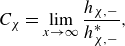 \begin{equation} C_\chi = \lim _{x \rightarrow \infty } \frac {h_{\chi , -}}{h^*_{\chi , -}}, \end{equation}
which implies an unitary modular, $|C_\chi |=1$
. We introduce a phase
$|C_\chi |=1$
. We introduce a phase $\phi _\chi$
to rewrite
$\phi _\chi$
to rewrite $C_\chi$
as
$C_\chi$
as
 \begin{equation} C_\chi = \textrm{e}^{2 \textrm{i}\phi _\chi }, \end{equation}
and define the sum and difference between the phases of $C_e$
and
$C_e$
and $C_o$
:
$C_o$
:
 \begin{equation} \phi _{\textit{s}} = \phi _e + \phi _o,\,\,\, \phi _{\textit{d}} = \phi _e - \phi _o. \end{equation}
Substituting (6.8) into (6.1) yields the transmission coefficient $T$
and reflection coefficient
$T$
and reflection coefficient $R$
expressed as
$R$
expressed as
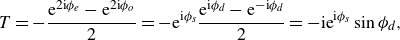 \begin{align} T &= - \frac {\textrm{e}^{2 \textrm{i}\phi _e} - \textrm{e}^{2 \textrm{i}\phi _o}}{2} = - \textrm{e}^{ \textrm{i}\phi _{\textit{s}}} \frac {\textrm{e}^{ \textrm{i}\phi _{\textit{d}} } - \textrm{e}^{- \textrm{i}\phi _{\textit{d}} }}{2} = - \textrm{ie}^{ \textrm{i}\phi _{\textit{s}}} \sin \phi _{\textit{d}} , \end{align}
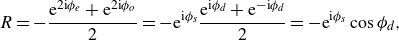 \begin{align} R &= - \frac {\textrm{e}^{2 \textrm{i}\phi _e} + \textrm{e}^{2 \textrm{i}\phi _o}}{2} = - \textrm{e}^{ \textrm{i}\phi _{\textit{s}}} \frac {\textrm{e}^{ \textrm{i}\phi _{\textit{d}} } + \textrm{e}^{- \textrm{i}\phi _{\textit{d}} }}{2} = - \textrm{e}^{ \textrm{i}\phi _{\textit{s}}} \cos \phi _{\textit{d}} , \\[6pt] \nonumber \end{align}
in which $\phi _d$
determines the magnitudes of
$\phi _d$
determines the magnitudes of $T$
and
$T$
and $R$
, and
$R$
, and $\phi _s$
determines the phases of
$\phi _s$
determines the phases of $T$
and
$T$
and $R$
. Recall that
$R$
. Recall that $\phi _d$
and
$\phi _d$
and $\phi _s$
are associated with the near fields
$\phi _s$
are associated with the near fields $h_e$
and
$h_e$
and $h_o$
.
$h_o$
.
It then follows from (6.9) that
 \begin{equation} |T|^2 + |R|^2 = 1, \end{equation}
as no energy dissipation occurs in either the fixed or free contact line conditions.
It also follows from (6.9) that, although the phases of $T$
and
$T$
and $R$
individually depend on
$R$
individually depend on $\phi _s$
associated with the near fields, the phase difference between
$\phi _s$
associated with the near fields, the phase difference between $T$
and
$T$
and $R$
does not rely on the near-field behaviours. The imaginary unit in (6.9a
) reveals that the phase of the transmission coefficient
$R$
does not rely on the near-field behaviours. The imaginary unit in (6.9a
) reveals that the phase of the transmission coefficient $T$
has a
$T$
has a $\pi /2$
phase difference compared with the reflection coefficient
$\pi /2$
phase difference compared with the reflection coefficient $R$
in (6.9b
):
$R$
in (6.9b
):
 \begin{equation} |\text{arg} \ T - \text{arg} \ R| = \frac {\pi }{2}. \end{equation}
7. Capillary–gravity waves: analytical solution for an infinitesimal barrier
For the infinitesimal barrier case, the radius of the cylindrical barrier is assumed to satisfy $r \rightarrow 0$
, implying that the barrier is much smaller than the characteristic wavelength of the incident waves. To maintain consistency with the linearised theory, this further requires that the surface displacement is sufficiently small, such that
$r \rightarrow 0$
, implying that the barrier is much smaller than the characteristic wavelength of the incident waves. To maintain consistency with the linearised theory, this further requires that the surface displacement is sufficiently small, such that $k \eta _A \ll r \ll 1$
. Under these assumptions, the liquid domain simplifies to the lower half-space
$k \eta _A \ll r \ll 1$
. Under these assumptions, the liquid domain simplifies to the lower half-space $H$
. Consequently, the BVP for
$H$
. Consequently, the BVP for $\phi$
, initially defined in (2.11), now transforms into
$\phi$
, initially defined in (2.11), now transforms into
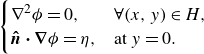 \begin{equation} \begin{cases} \displaystyle \nabla ^2 \phi = 0, & \forall (x, y) \in H, \\ \displaystyle \boldsymbol{\hat {n}} \boldsymbol{\cdot } \boldsymbol{\nabla } \phi = \eta , & \text{at } y = 0. \end{cases} \end{equation}
Similarly, the BVPs for $\eta$
(2.12) modify as follows:
$\eta$
(2.12) modify as follows:
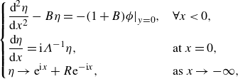 \begin{equation} \begin{cases} \displaystyle \frac {\textrm{d}^2 \eta }{\textrm{d}x^2} - B \eta = - (1+B) \phi \big |_{y=0}, & \forall x \lt 0, \\[8pt] \displaystyle \frac {\textrm{d} \eta }{\textrm{d}x} = \textrm{i}\Lambda ^{-1} \eta , & \text{at } x = 0, \\[5pt] \displaystyle \eta \rightarrow \textrm{e}^{\textrm{i}x} + R \textrm{e}^{-\textrm{i}x}, & \text{as } x \rightarrow -\infty , \end{cases} \end{equation}
and
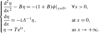 \begin{equation} \begin{cases} \displaystyle \frac {\textrm{d}^2 \eta }{\textrm{d}x^2} - B \eta = - (1+B) \phi \big |_{y=0}, & \forall x \gt 0, \\[8pt] \displaystyle \frac {\textrm{d} \eta }{\textrm{d}x} = - \textrm{i}\Lambda ^{-1} \eta , & \text{at } x = 0, \\[5pt] \displaystyle \eta \rightarrow T \textrm{e}^{ \textrm{i}x }, & \text{as } x \rightarrow +\infty . \end{cases} \end{equation}
Given that $H$
itself is the liquid domain, no transformation into a lower half-space is required. Thus, the conformal mapping
$H$
itself is the liquid domain, no transformation into a lower half-space is required. Thus, the conformal mapping $w = z/r + r/z$
in § 3.2.1 simplifies to the identity
$w = z/r + r/z$
in § 3.2.1 simplifies to the identity $w = z$
. Employing a similar approach as in § 3.2.2, we formulate the integral equation problem for
$w = z$
. Employing a similar approach as in § 3.2.2, we formulate the integral equation problem for $f(x) = \phi (x, 0)$
:
$f(x) = \phi (x, 0)$
:
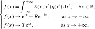 \begin{equation} \begin{cases} \displaystyle f(x) = \int _{-\infty }^{+\infty } S (x, x') \eta (x') \: \textrm{d} x' , \quad \forall x \in \mathbb{R}, \\[3pt] \displaystyle f(x) \rightarrow \textrm{e}^{\textrm{i}x} + R \textrm{e}^{-\textrm{i}x}, \qquad \ \text{as } x \rightarrow -\infty , \\[3pt] \displaystyle f(x) \rightarrow T \textrm{e}^{\textrm{i}x}, \quad \qquad \qquad \text{as } x \rightarrow +\infty , \end{cases} \end{equation}
where $S$
is defined by
$S$
is defined by
 \begin{equation} S (x, x') = - \pi ^{-1} \left ( \ln { \left | x - x' \right | } + \gamma \right ). \end{equation}
Following the analysis in §§ 4.1 and 4.2, we derive the equations for $h_{\chi , \pm }$
:
$h_{\chi , \pm }$
:
 \begin{equation} h_{\chi , \pm } = \mathcal{L}_{\chi } \mathcal{K} h_{\chi ,\pm } + (\mathcal{L}_{\chi } \mathcal{K} - \mathcal{I}) \textrm{e}^{\pm \textrm{i}x} , \end{equation}
where the kernels for $\mathcal{L}_{\chi }$
are redefined as follows:
$\mathcal{L}_{\chi }$
are redefined as follows:
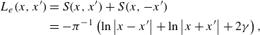 \begin{align} L_e(x,x') & = S (x, x') + S (x, -x') \nonumber \\ &= - \pi ^{-1} \left ( \ln \left | x - x' \right | + \ln \left | x + x' \right | + 2 \gamma \right ) , \end{align}
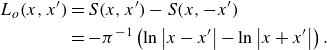 \begin{align} L_o(x,x') &= S (x, x') - S (x, -x') \nonumber \\ &= - \pi ^{-1} \left ( \ln \left | x - x' \right | - \ln \left | x + x' \right | \right ) . \\[6pt] \nonumber \end{align}
and the kernel for $\mathcal{K}$
updates to
$\mathcal{K}$
updates to
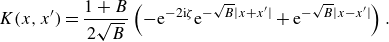 \begin{equation} K(x, x') = \frac {1+B}{2\sqrt {B}} \left ( -\textrm{e}^{-2\textrm{i}\zeta } \textrm{e}^{- \sqrt {B}|x + x'|} + \textrm{e}^{-\sqrt {B}|x - x'|} \right ). \end{equation}
The solution to (7.5) can be obtained using Fourier cosine and sine transforms. The detailed derivation and mathematical techniques are provided in Appendix D. The derived solutions for $h_{e, \pm }$
and
$h_{e, \pm }$
and $h_{o, \pm }$
facilitate the calculation of transmission
$h_{o, \pm }$
facilitate the calculation of transmission $T$
and reflection
$T$
and reflection $R$
coefficients, as delineated in (4.14). These coefficients are expressed as
$R$
coefficients, as delineated in (4.14). These coefficients are expressed as
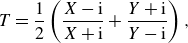 \begin{align} T &= \frac {1}{2} \left ( \frac {X-\textrm{i}}{X+\textrm{i}} + \frac {Y+\textrm{i}}{Y-\textrm{i}} \right ) , \end{align}
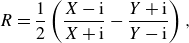 \begin{align} R &= \frac {1}{2} \left ( \frac {X-\textrm{i}}{X+\textrm{i}} - \frac {Y+\textrm{i}}{Y-\textrm{i}} \right ) , \end{align}
where
 \begin{align}&\,\,\, X = \frac {1}{\pi } \left (\frac {3 + 2B}{\sqrt {3 + 4B}} \tan ^{-1}\left (\sqrt {3 + 4B}\right ) + \frac {1}{2} \ln (1 + B)\right ) + \textrm{i}\frac {(3 + B) \tan \zeta }{2 \sqrt {B}} , \end{align}
 \begin{align}& Y = \frac {1}{\pi } \left (\frac {3 + 6B + 2B^2}{\sqrt {3 + 4B}} \tan ^{-1}\left (\sqrt {3 + 4B}\right ) - \frac {1}{2} \ln (1 + B)\right ) - \textrm{i}\frac {(3 + B) \sqrt {B}}{2 \tan \zeta } . \end{align}
This solution expresses $T$
and
$T$
and $R$
as functions of the dimensionless Bond number
$R$
as functions of the dimensionless Bond number $B$
defined in (2.6) and dimensionless slip parameter
$B$
defined in (2.6) and dimensionless slip parameter $\zeta$
defined in (3.3).
$\zeta$
defined in (3.3).
In Hocking’s work (Hocking Reference Hocking1987b
) considering scattering from an infinitesimally thin barrier of a finite immersed depth, an analytical solution arises in the limit of a zero immersed depth $d \rightarrow 0$
. In contrast, our solution is derived from a cylindrical barrier geometry, reducing to an infinitesimal barrier as the radius
$d \rightarrow 0$
. In contrast, our solution is derived from a cylindrical barrier geometry, reducing to an infinitesimal barrier as the radius $r \rightarrow 0$
. In Appendix E, we show that the two solutions are equivalent even though they approach an infinitesimal barrier in different ways. Our theory underscores a generalisation from an idealised infinitesimally thin barrier to a cylindrical barrier of practical applicability.
$r \rightarrow 0$
. In Appendix E, we show that the two solutions are equivalent even though they approach an infinitesimal barrier in different ways. Our theory underscores a generalisation from an idealised infinitesimally thin barrier to a cylindrical barrier of practical applicability.
7.1. Fixed contact line
For the case of infinitesimal barrier ( $r \rightarrow 0$
) with a fixed contact line (
$r \rightarrow 0$
) with a fixed contact line ( $\zeta = 0$
), (7.8) reduce to
$\zeta = 0$
), (7.8) reduce to
 \begin{align}&\,\, T = \frac {1}{2} \left ( \frac {X-\textrm{i}}{X+\textrm{i}} + 1 \right ) =\frac {X}{X+\textrm{i}}, \end{align}
 \begin{align}& R = \frac {1}{2} \left ( \frac {X-\textrm{i}}{X+\textrm{i}} - 1 \right ) = - \frac {\textrm{i}}{X+\textrm{i}} , \end{align}
where
 \begin{equation} X = \frac {1}{\pi } \left (\frac {3 + 2B}{\sqrt {3 + 4B}} \tan ^{-1}\left (\sqrt {3 + 4B}\right ) + \frac {1}{2} \ln (1 + B)\right ) . \end{equation}
Here, $R$
and
$R$
and $T$
satisfies the
$T$
satisfies the $90^\circ$
phase difference revealed in the prior section.
$90^\circ$
phase difference revealed in the prior section.
It follows from (7.9) that
 \begin{equation} R = T - 1, \end{equation}
implying that the diffracted field, $\phi _D = \phi - \phi _I$
, is symmetric about the barrier, that is,
$\phi _D = \phi - \phi _I$
, is symmetric about the barrier, that is,
 \begin{equation} \phi _D(x, y) = \phi _D(-x, y). \end{equation}
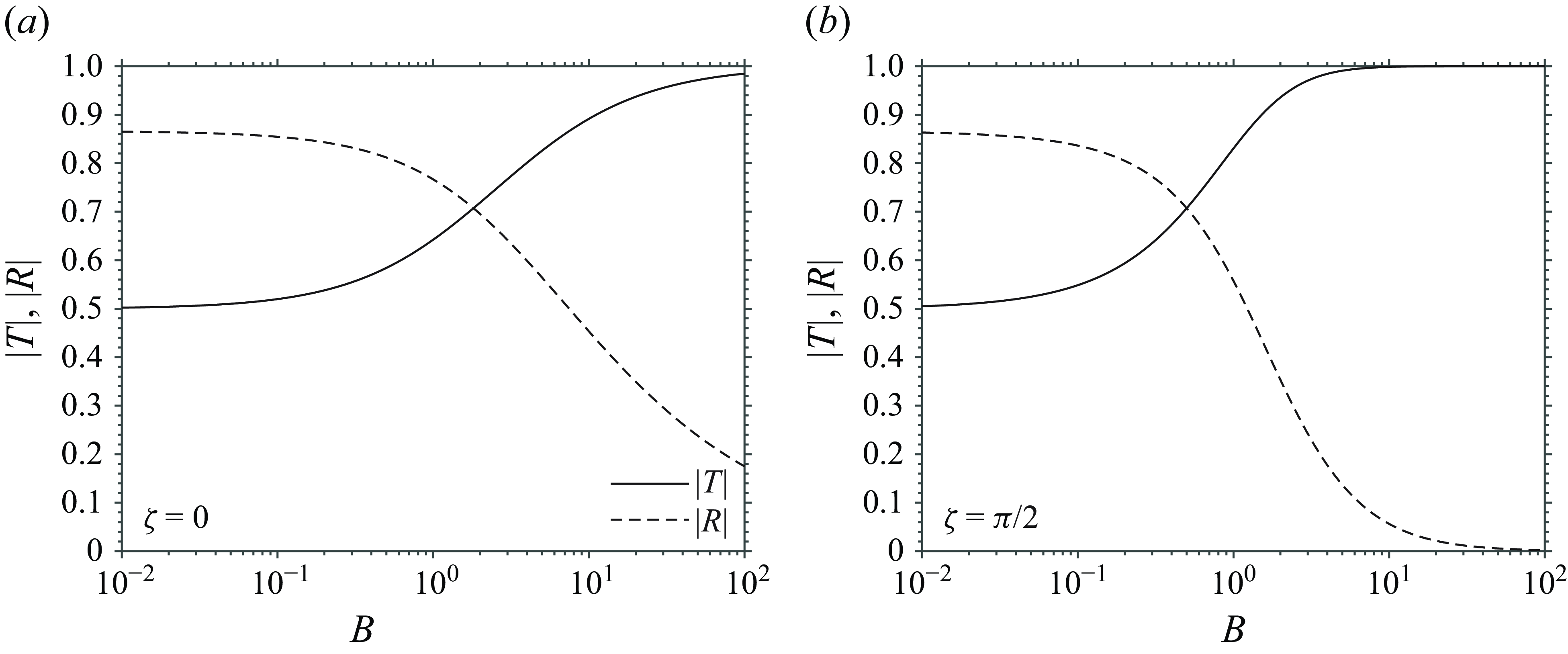
Figure 4. Transmission $|T|$
and reflection
$|T|$
and reflection $|R|$
as functions of the Bond number
$|R|$
as functions of the Bond number $B$
(defined in (2.6)) when scattered by an infinitesimal barrier
$B$
(defined in (2.6)) when scattered by an infinitesimal barrier $r=0$
: (a) fixed and (b) free contact lines, following from (7.9) and (7.12), respectively. The dimensionless slip parameter
$r=0$
: (a) fixed and (b) free contact lines, following from (7.9) and (7.12), respectively. The dimensionless slip parameter $\zeta$
is defined in (3.3).
$\zeta$
is defined in (3.3).
7.2. Free contact line
For the case of infinitesimal barrier ( $r \rightarrow 0$
) with a free contact line (
$r \rightarrow 0$
) with a free contact line ( $\zeta = \pi /2$
), (7.8) reduce to
$\zeta = \pi /2$
), (7.8) reduce to
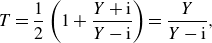 \begin{align} T &= \frac {1}{2} \left ( 1 + \frac {Y+\textrm{i}}{Y-\textrm{i}} \right ) = \frac {Y}{Y-\textrm{i}}, \end{align}
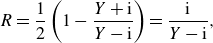 \begin{align} R &= \frac {1}{2} \left ( 1 - \frac {Y+\textrm{i}}{Y-\textrm{i}} \right ) = \frac {\textrm{i}}{Y-\textrm{i}} , \end{align}
where
 \begin{equation} Y = \frac {1}{\pi } \left (\frac {3 + 6B + 2B^2}{\sqrt {3 + 4B}} \tan ^{-1}\left (\sqrt {3 + 4B}\right ) - \frac {1}{2} \ln (1 + B)\right ) , \end{equation}
Again, $R$
and
$R$
and $T$
satisfies the
$T$
satisfies the $90^\circ$
phase difference revealed in the prior section.
$90^\circ$
phase difference revealed in the prior section.
It follows from (7.12) that
 \begin{equation} -R = T - 1 , \end{equation}
implying that the diffracted field, $\phi _D = \phi - \phi _I$
, is anti-symmetric about the barrier, that is,
$\phi _D = \phi - \phi _I$
, is anti-symmetric about the barrier, that is,
 \begin{equation} \phi _D(x, y) = - \phi _D(-x, y). \end{equation}
8. From an infinitesimal barrier to a barrier with a finite cross-section: no dissipation
The transmission properties of surface waves interacting with an infinitesimal barrier, as calculated from the closed-form solution (7.9) and (7.12), are shown in figure 4, revealing distinct behaviours depending on the Bond number. Figure 4(a) presents the magnitudes of transmission $|T|$
and reflection
$|T|$
and reflection $|R|$
as functions of the Bond number
$|R|$
as functions of the Bond number $B$
with a fixed contact line (
$B$
with a fixed contact line ( $\zeta = 0$
). In the capillary limit (
$\zeta = 0$
). In the capillary limit ( $B \ll 1$
), the transmission coefficient asymptotically approaches
$B \ll 1$
), the transmission coefficient asymptotically approaches $|T| = 0.5$
, indicating that only 25 % of the capillary wave energy is transmitted, while the remaining 75 % energy driven by surface tension is reflected by the fixed contact lines. As the system transitions to the gravity-dominated regime (
$|T| = 0.5$
, indicating that only 25 % of the capillary wave energy is transmitted, while the remaining 75 % energy driven by surface tension is reflected by the fixed contact lines. As the system transitions to the gravity-dominated regime ( $B \gg 1$
), the influence of the contact line diminishes and the transmission approaches
$B \gg 1$
), the influence of the contact line diminishes and the transmission approaches $|T| = 1$
. In this regime, the barrier no longer significantly affects the wave, allowing the full wave energy to pass through.
$|T| = 1$
. In this regime, the barrier no longer significantly affects the wave, allowing the full wave energy to pass through.
Figure 4(b) shows the results for a free contact line ( $\zeta = \pi /2$
). The behaviour in the capillary and gravity limits (
$\zeta = \pi /2$
). The behaviour in the capillary and gravity limits ( $B \ll 1$
and
$B \ll 1$
and $B \gg 1$
) are similar to the fixed contact line case, with the transmission coefficient approaching
$B \gg 1$
) are similar to the fixed contact line case, with the transmission coefficient approaching $|T| = 0.5$
and 1, respectively. However, in the intermediate Bond number range, the free contact lines allow for the transmission greater than that of the fixed contact lines, as depicted by a comparison between figures 4(a) and 4(b). Such a transmission difference between the two cases follows from different coupling of the energy from the incident side to the transmitted side, as evident in the symmetry difference of the diffracted fields between the two cases, as noted earlier in (7.11) versus (7.14).
$|T| = 0.5$
and 1, respectively. However, in the intermediate Bond number range, the free contact lines allow for the transmission greater than that of the fixed contact lines, as depicted by a comparison between figures 4(a) and 4(b). Such a transmission difference between the two cases follows from different coupling of the energy from the incident side to the transmitted side, as evident in the symmetry difference of the diffracted fields between the two cases, as noted earlier in (7.11) versus (7.14).
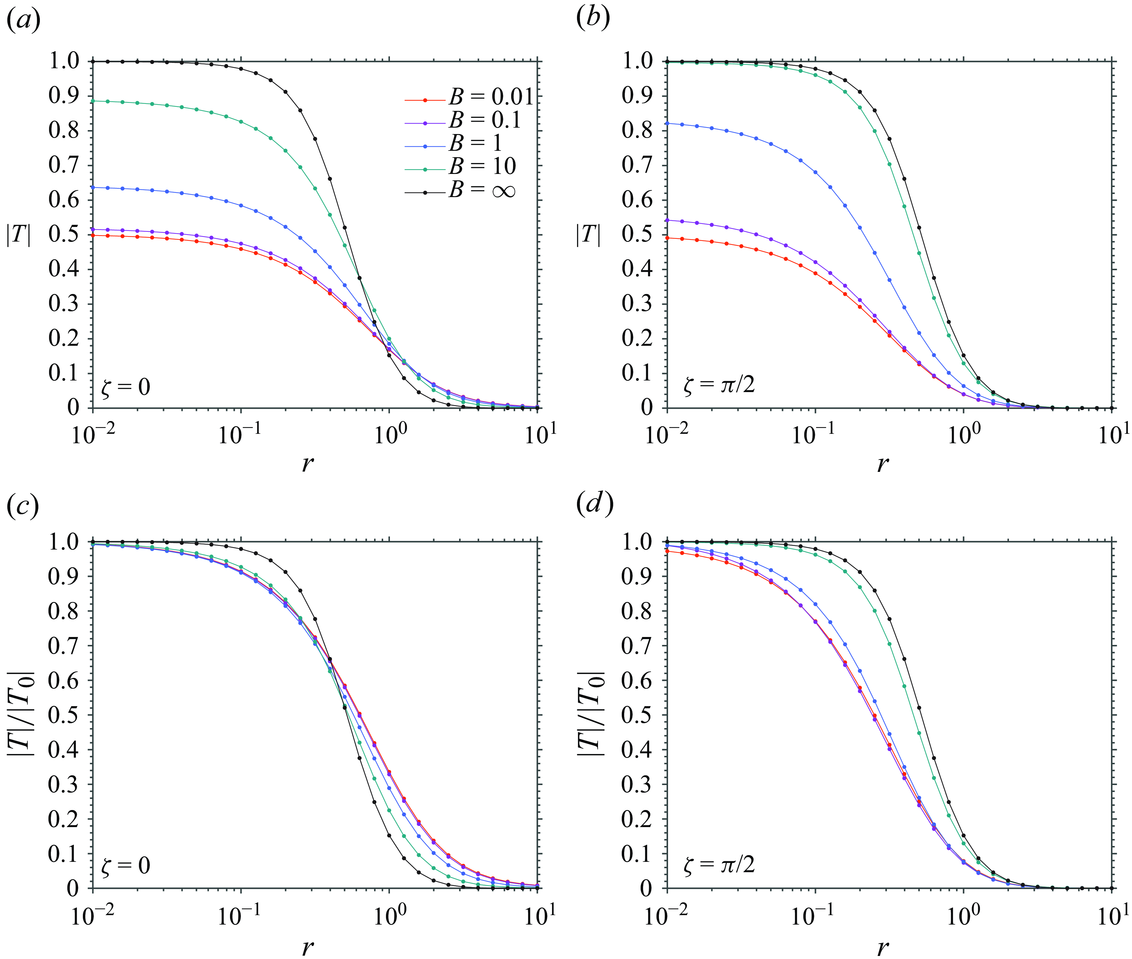
Figure 5. (a) and (b) Transmission coefficient $|T|$
as a function of the dimensionless barrier radius
$|T|$
as a function of the dimensionless barrier radius $r$
for different Bond number values for fixed and free contact lines,
$r$
for different Bond number values for fixed and free contact lines, $\zeta = 0$
and
$\zeta = 0$
and $\pi /2$
, respectively. Panels (c) and (d) are the same as panels (a) and (b), respectively, but with the transmission coefficient
$\pi /2$
, respectively. Panels (c) and (d) are the same as panels (a) and (b), respectively, but with the transmission coefficient $|T|$
normalised by the transmission in the infinitesimal barrier limit
$|T|$
normalised by the transmission in the infinitesimal barrier limit $|T_0|$
.
$|T_0|$
.
As the barrier is increased from zero size to a finite cylindrical geometry, the transmission depends on the Bond number and barrier size. For a range of Bond number $B$
values, the transmission coefficient is calculated from the semi-analytical method using (4.14a
) and illustrated in figures 5(a) and 5(b) for dependence on the dimensionless barrier radius (
$B$
values, the transmission coefficient is calculated from the semi-analytical method using (4.14a
) and illustrated in figures 5(a) and 5(b) for dependence on the dimensionless barrier radius ( $r=kr'$
). In the limit of small barrier sizes (
$r=kr'$
). In the limit of small barrier sizes ( $r \ll 1$
), the transmission
$r \ll 1$
), the transmission $|T|$
approaches values ranging from 0.5 to 1 when varying the Bond number from the capillary-dominant regime (
$|T|$
approaches values ranging from 0.5 to 1 when varying the Bond number from the capillary-dominant regime ( $B \ll 1$
) to gravity-dominant regime (
$B \ll 1$
) to gravity-dominant regime ( $B \gg 1$
), as noted earlier in figure 4. As the barrier radius becomes larger (
$B \gg 1$
), as noted earlier in figure 4. As the barrier radius becomes larger ( $r \gg 1$
), the transmission coefficient across different Bond number values uniformly decreases due to the barrier’s finite cross-section. Compared with the fixed contact line, the overall transmission
$r \gg 1$
), the transmission coefficient across different Bond number values uniformly decreases due to the barrier’s finite cross-section. Compared with the fixed contact line, the overall transmission $|T|$
is higher for all
$|T|$
is higher for all $B$
under the free contact line.
$B$
under the free contact line.
There is an interplay of Bond number and barrier size. For the fixed contact lines (figure 5
a), the transmission showcases a contrast when the radius $r$
crosses around 1: at small
$r$
crosses around 1: at small $r$
, higher
$r$
, higher $B$
leads to higher transmission, but at large
$B$
leads to higher transmission, but at large $r$
, lower
$r$
, lower $B$
results in higher transmission. In contrast, for the free contact lines (figure 5
b), the barrier size effect appears uniform across different
$B$
results in higher transmission. In contrast, for the free contact lines (figure 5
b), the barrier size effect appears uniform across different $B$
: the higher the
$B$
: the higher the $B$
, the higher the transmission. If we normalise the transmission
$B$
, the higher the transmission. If we normalise the transmission $|T|$
by the infinitesimal-barrier limit
$|T|$
by the infinitesimal-barrier limit $|T_0|$
(from the closed-form solution (7.8a
)), the ratio
$|T_0|$
(from the closed-form solution (7.8a
)), the ratio $|T| / |T_0|$
highlights the size effect across different Bond numbers.
$|T| / |T_0|$
highlights the size effect across different Bond numbers.
The influence of barrier size as examined by the normalised transmission $|T|/|T_0|$
is now shown in figures 5(c) and 5(d). The results show that for small barrier radii (
$|T|/|T_0|$
is now shown in figures 5(c) and 5(d). The results show that for small barrier radii ( $r\lt 0.1$
), the effect of barrier size is minimal, reducing transmission by no more than 10 %. However, as the barrier radius becomes comparable to the wavelength (
$r\lt 0.1$
), the effect of barrier size is minimal, reducing transmission by no more than 10 %. However, as the barrier radius becomes comparable to the wavelength ( $0.1 \lt r \lt 1$
), transmission decreases substantially, pointing to a more significant interaction between the wave and the barrier. For large barriers (
$0.1 \lt r \lt 1$
), transmission decreases substantially, pointing to a more significant interaction between the wave and the barrier. For large barriers ( $r \gt 1$
), transmission is reduced to less than 20 %, indicating a dramatic size effect. These findings demonstrate a clear size-dependent transmission behaviour, regardless of the Bond number. All key observations in this section have been summarised in table 1.
$r \gt 1$
), transmission is reduced to less than 20 %, indicating a dramatic size effect. These findings demonstrate a clear size-dependent transmission behaviour, regardless of the Bond number. All key observations in this section have been summarised in table 1.
Table 1. Summary of transmission behaviours for various Bond numbers ( $B$
) and barrier radii (
$B$
) and barrier radii ( $r$
) at the cases of fixed and free contact lines. The dimensionless slip parameter
$r$
) at the cases of fixed and free contact lines. The dimensionless slip parameter $\zeta$
is defined in (3.3).
$\zeta$
is defined in (3.3).
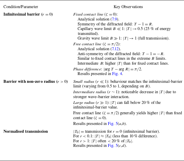
9. Dissipation due to dynamic contact lines
For general contact line dynamics with a finite slip coefficient $\Lambda '$
, energy dissipation occurs near the contact lines due to the slipping motion. In our model, which analyses the scattering of capillary–gravity waves by a fixed, semi-immersed cylindrical barrier with dynamic contact lines, this dissipation depends on the dimensionless barrier radius
$\Lambda '$
, energy dissipation occurs near the contact lines due to the slipping motion. In our model, which analyses the scattering of capillary–gravity waves by a fixed, semi-immersed cylindrical barrier with dynamic contact lines, this dissipation depends on the dimensionless barrier radius $r$
, the Bond number
$r$
, the Bond number $B$
and the slip parameter
$B$
and the slip parameter $\zeta$
. We are interested in finding the slip coefficient values where the dissipation is most effective.
$\zeta$
. We are interested in finding the slip coefficient values where the dissipation is most effective.

Figure 6. Intensity plots of (a) energy dissipation $1 - |T|^2 - |R|^2$
, (b) phase difference
$1 - |T|^2 - |R|^2$
, (b) phase difference $\arg T - \arg R$
, (c) transmission
$\arg T - \arg R$
, (c) transmission $|T|$
and (d) reflection
$|T|$
and (d) reflection $|R|$
in the parameter space of the Bond number
$|R|$
in the parameter space of the Bond number $B$
and the slip parameter
$B$
and the slip parameter $\zeta$
(defined in (3.3)) for scattering in the infinitesimal barrier limit, following from (7.8). The black dashed line represents the slip coefficient values where maximum dissipation occurs at given
$\zeta$
(defined in (3.3)) for scattering in the infinitesimal barrier limit, following from (7.8). The black dashed line represents the slip coefficient values where maximum dissipation occurs at given $B$
, and is compared with the white dash-dotted line and the white dotted line, representing the slip coefficient equal to the phase speed of capillary waves from (9.1) and the phase speed of capillary–gravity waves from (9.2), respectively. The black solid line indicates the ridge of dissipation, representing the path of the least descent for the dissipation in the parameter space of
$B$
, and is compared with the white dash-dotted line and the white dotted line, representing the slip coefficient equal to the phase speed of capillary waves from (9.1) and the phase speed of capillary–gravity waves from (9.2), respectively. The black solid line indicates the ridge of dissipation, representing the path of the least descent for the dissipation in the parameter space of $B$
and
$B$
and $\zeta$
, and coincides with the white dashed line from (9.3).
$\zeta$
, and coincides with the white dashed line from (9.3).
For an infinitesimal barrier ( $r \ll 1$
), the results are presented in the parameter space of
$r \ll 1$
), the results are presented in the parameter space of $B$
and
$B$
and $\zeta$
(figure 6) in terms of partition of energy dissipation
$\zeta$
(figure 6) in terms of partition of energy dissipation $E_s = 1 - |T|^2 - |R|^2$
, phase relation
$E_s = 1 - |T|^2 - |R|^2$
, phase relation $\arg T - \arg R$
, transmission
$\arg T - \arg R$
, transmission $|T|$
and reflection
$|T|$
and reflection $|R|$
, calculated from (7.8). In figure 6, the slip coefficient for maximum dissipation at a given Bond number
$|R|$
, calculated from (7.8). In figure 6, the slip coefficient for maximum dissipation at a given Bond number $B$
is shown by the black dashed line. We also include two reference lines: the condition where the slip coefficient
$B$
is shown by the black dashed line. We also include two reference lines: the condition where the slip coefficient $\Lambda '$
equals the phase speed of pure capillary waves (white dash-dotted line),
$\Lambda '$
equals the phase speed of pure capillary waves (white dash-dotted line),
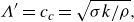 \begin{equation} \Lambda ' = c_c = \sqrt {\sigma k / \rho }, \end{equation}
corresponding to
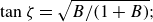 \begin{equation} \tan \zeta = \sqrt {B/(1+B)}; \end{equation}
and the condition where the slip coefficient $\Lambda '$
equals phase speed of capillary–gravity waves (white dotted line),
$\Lambda '$
equals phase speed of capillary–gravity waves (white dotted line),
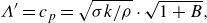 \begin{equation} \Lambda ' = c_p = \sqrt {\sigma k / \rho } \cdot \sqrt {1+B}, \end{equation}
corresponding to
 \begin{equation} \tan \zeta = \sqrt {B}. \end{equation}
For small $B$
, the two reference lines align closely with the calculated maximum dissipation line. However, as
$B$
, the two reference lines align closely with the calculated maximum dissipation line. However, as $B$
increases, the maximum dissipation line deviates from both reference lines, but remains closer to the
$B$
increases, the maximum dissipation line deviates from both reference lines, but remains closer to the $\Lambda ' = c_c$
line. This behaviour can be interpreted by wave impedance matching with the impedance of the contact line motion. The results suggest that the incident energy is more effectively coupled to the contact line boundary when
$\Lambda ' = c_c$
line. This behaviour can be interpreted by wave impedance matching with the impedance of the contact line motion. The results suggest that the incident energy is more effectively coupled to the contact line boundary when $\Lambda '$
is closer to the phase speed of the pure capillary wave (
$\Lambda '$
is closer to the phase speed of the pure capillary wave ( $c_c$
) than the capillary–gravity wave (
$c_c$
) than the capillary–gravity wave ( $c_p$
). This proximity to
$c_p$
). This proximity to $\Lambda ' = c_c$
reflects the dominant role of surface tension effects in determining energy dissipation at any Bond numbers. The results extend a finding of Zhang & Thiessen (Reference Zhang and Thiessen2013) that, in the limit of pure capillary waves (
$\Lambda ' = c_c$
reflects the dominant role of surface tension effects in determining energy dissipation at any Bond numbers. The results extend a finding of Zhang & Thiessen (Reference Zhang and Thiessen2013) that, in the limit of pure capillary waves ( $B \rightarrow 0$
) and infinitesimal barrier (
$B \rightarrow 0$
) and infinitesimal barrier ( $r\rightarrow 0$
), maximum dissipation occurs when the slip coefficient
$r\rightarrow 0$
), maximum dissipation occurs when the slip coefficient $\Lambda '$
equals the phase speed of the incident capillary waves. Extending this analysis, we examine energy dissipation beyond pure capillary waves, incorporating an arbitrary Bond number
$\Lambda '$
equals the phase speed of the incident capillary waves. Extending this analysis, we examine energy dissipation beyond pure capillary waves, incorporating an arbitrary Bond number $B$
.
$B$
.
Also shown in figure 6(a) is the ridge of dissipation (black solid line), following from the minima of the magnitude of the gradients of the dissipation in the parameter space. The line represents the path of least descent for dissipation in the parameter space. Intriguingly, it is observed that this dissipation ridge line fits with the relation (white dashed line)
 \begin{equation} \Lambda ' = \sqrt {\sigma k / \rho } \cdot \sqrt {(1+B)/(1-B)}, \end{equation}
corresponding to
 \begin{equation} \tan \zeta = \sqrt {B/(1-B)}. \end{equation}
The physical interpretation of this coincidence remains unclear and warrants further investigation. The phase difference $\arg T - \arg R$
depicted in figure 6(b), generally differing from
$\arg T - \arg R$
depicted in figure 6(b), generally differing from $90^\circ$
with the dissipation, crosses
$90^\circ$
with the dissipation, crosses $90^\circ$
around the ridge of the dissipation.
$90^\circ$
around the ridge of the dissipation.

Figure 7. Intensity plots of (a) $1 - |T|^2 - |R|^2$
, (b)
$1 - |T|^2 - |R|^2$
, (b) $\arg T - \arg R$
, (c)
$\arg T - \arg R$
, (c) $|T|$
and (d)
$|T|$
and (d) $|R|$
in the parameter space of the dimensionless barrier radius
$|R|$
in the parameter space of the dimensionless barrier radius $r$
and slip parameter
$r$
and slip parameter $\zeta$
for a Bond number
$\zeta$
for a Bond number $B = 1$
. The dashed lines correspond to (a) a maximum
$B = 1$
. The dashed lines correspond to (a) a maximum $1 - |T|^2 - |R|^2$
, (b) a
$1 - |T|^2 - |R|^2$
, (b) a $90^\circ$
phase difference, (c) a minimum
$90^\circ$
phase difference, (c) a minimum $|T|$
and (d) a minimum
$|T|$
and (d) a minimum $|R|$
at given
$|R|$
at given $B$
.
$B$
.
As the barrier size increases from zero to a finite value, the calculated results of the dissipation partition $E_s$
, phase difference
$E_s$
, phase difference $\arg T - \arg R$
, transmission
$\arg T - \arg R$
, transmission $|T|$
and reflection
$|T|$
and reflection $|R|$
are presented in figure 7 in the parameter space of
$|R|$
are presented in figure 7 in the parameter space of $r$
and
$r$
and $\zeta$
for a Bond number
$\zeta$
for a Bond number $B = 1$
, a typical value when surface tension and gravity effects are comparable. The results of the dissipation partition in figure 7(a) show that contact line dissipation remains significant even as the barrier size increases. The slip parameter
$B = 1$
, a typical value when surface tension and gravity effects are comparable. The results of the dissipation partition in figure 7(a) show that contact line dissipation remains significant even as the barrier size increases. The slip parameter $\zeta$
corresponding to maximum dissipation for a given
$\zeta$
corresponding to maximum dissipation for a given $r$
stays near
$r$
stays near $0.2\pi$
across the range of
$0.2\pi$
across the range of $r$
, where the dissipation remains approximately
$r$
, where the dissipation remains approximately $80\,\%$
. Increasing the barrier size has little effect on the overall energy dissipation, as the dissipation is due to the contact lines and is largely independent of the barrier size. Nevertheless, the phase difference is sensitive to the size, as depicted in figure 7(b).
$80\,\%$
. Increasing the barrier size has little effect on the overall energy dissipation, as the dissipation is due to the contact lines and is largely independent of the barrier size. Nevertheless, the phase difference is sensitive to the size, as depicted in figure 7(b).
Even though the barrier size has little effect on the overall energy dissipation, the transmission and reflection individually have a strong dependence on the size. The transmission shown in figure 7(c) highlights a significant reduction as the barrier radius increases, particularly for $r \gt 1$
, where the barrier size becomes comparable to the wavelength for the transmission to diminish to nearly negligible levels. This sharp decrease underscores the dominance of reflection and/or dissipation when the barrier size exceeds the wavelength scale. Also shown is the slip parameter
$r \gt 1$
, where the barrier size becomes comparable to the wavelength for the transmission to diminish to nearly negligible levels. This sharp decrease underscores the dominance of reflection and/or dissipation when the barrier size exceeds the wavelength scale. Also shown is the slip parameter $\zeta$
for the minimum transmission for a given
$\zeta$
for the minimum transmission for a given $r$
(white dashed line), which changes from
$r$
(white dashed line), which changes from $0.17 \pi$
to
$0.17 \pi$
to $0.5 \pi$
, with particularly rapid variation near
$0.5 \pi$
, with particularly rapid variation near $r = 1$
.
$r = 1$
.
The reflection, depicted in figure 7(d), generally increases with increasing size $r$
. The value of
$r$
. The value of $\zeta$
corresponding to minimum reflection for a given
$\zeta$
corresponding to minimum reflection for a given $r$
gradually shifts from
$r$
gradually shifts from $0.25 \pi$
to
$0.25 \pi$
to $0.18 \pi$
. This indicates that the reflection is less sensitive to changes in barrier size compared with transmission, which could imply a relatively stable reflection behaviour over a range of barrier sizes.
$0.18 \pi$
. This indicates that the reflection is less sensitive to changes in barrier size compared with transmission, which could imply a relatively stable reflection behaviour over a range of barrier sizes.
Overall, results from figure 7 suggest that while the transmission is heavily affected by increasing barrier size, dissipation and reflection exhibit more complex but less drastic changes. The interplay between $r$
and
$r$
and $\zeta$
across the different plots provides a comprehensive view of the wave dynamics influenced by the barrier. All key observations in this section have been summarised in table 2.
$\zeta$
across the different plots provides a comprehensive view of the wave dynamics influenced by the barrier. All key observations in this section have been summarised in table 2.
Table 2. Summary of dissipation properties and wave transmission/reflection for dynamic contact lines. Parameters: Bond number $B$
, slip parameter
$B$
, slip parameter $\zeta$
and barrier radius
$\zeta$
and barrier radius $r$
.
$r$
.
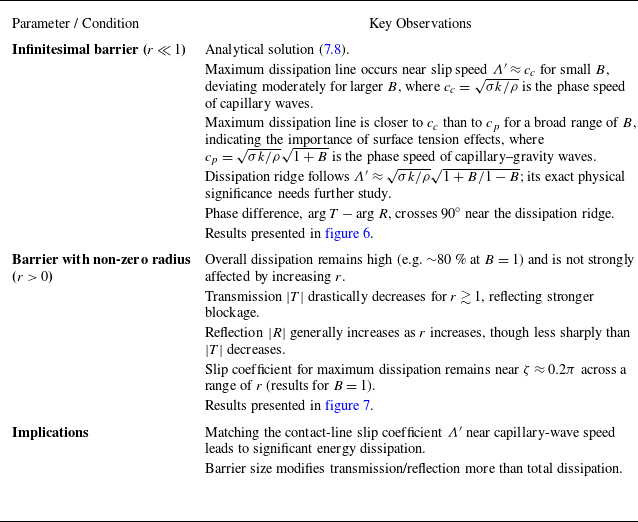
10. Summary and discussion
This study develops a comprehensive semi-analytical framework to investigate the scattering of capillary–gravity waves by a fixed, semi-immersed cylindrical barrier while incorporating the dynamic contact line condition. The formulation begins with the linearised potential flow assumption, leveraging an effective-slip model to connect the contact line velocity and the deviation of the contact angle from its equilibrium state. This approach extends classical theories of pure gravity wave scattering by a thin barrier to include the effect of surface tension, dynamic contact lines and a cylindrical barrier geometry with non-zero cross-section, thereby providing a more complete representation of realistic wave–barrier interactions.
Two coupled boundary value problems regarding the velocity potential and surface elevation, formulated from the governing equations and boundary conditions, are solved using techniques such as differential equations, conformal mapping and Fourier transforms. These problems are combined into a compound integral equation, which is simplified using advanced integral equation techniques and then numerically solved via discretisation with the Nyström method. Numerous integrals were analytically resolved using specialised techniques to streamline the formulation.
Benchmarking against prior pure-gravity results validates the consistency and accuracy of the theoretical framework. Under the limiting cases of fixed and free contact line conditions, our analysis of capillary–gravity wave scattering revisits the fundamental energy-conserving behaviours and reveals a $90^\circ$
phase difference between the transmission and reflection coefficients,
$90^\circ$
phase difference between the transmission and reflection coefficients, $T$
and
$T$
and $R$
.
$R$
.
A key theoretical contribution of our analysis of capillary–gravity wave scattering is the closed-form solution (7.8) derived for an infinitesimal barrier using Fourier cosine and sine transforms, along with advanced integral equation techniques. This solution reveals that the diffracted field is symmetric or anti-symmetric between the incident and transmitted sides under fixed or free contact line conditions of no dissipation, respectively. The analysis for no dissipation also characterises reduced transmission ( $|T_0|$
) varying from 1 to 0.5 as the waves transition from gravity waves to capillary waves. This analytical result then serves as a baseline for illustrating how scattering characteristics evolve from an infinitesimal barrier radius to larger barrier radii using the ratio
$|T_0|$
) varying from 1 to 0.5 as the waves transition from gravity waves to capillary waves. This analytical result then serves as a baseline for illustrating how scattering characteristics evolve from an infinitesimal barrier radius to larger barrier radii using the ratio $|T|/|T_0|$
, providing insights into the transition from nearly unimpeded wave propagation (
$|T|/|T_0|$
, providing insights into the transition from nearly unimpeded wave propagation ( $|T|/|T_0|=1$
) to regimes where the barrier significantly alters the transmission.
$|T|/|T_0|=1$
) to regimes where the barrier significantly alters the transmission.
Our analysis of energy dissipation due to dynamic contact lines reveals the effects of barrier radius, Bond number and slip coefficient in capillary–gravity wave scattering. For an infinitesimal barrier, the maximum dissipation occurs when the slip coefficient approximates the phase speed of capillary waves given by (9.1), supporting previous findings for impedance matching between pure capillary waves and contact line motions while extending the analysis to arbitrary Bond numbers. In the parameter space of Bond number and slip parameter, the dissipation ridge, representing the path of least descent, was found to coincide with a special relation given in (9.3), where the phase difference crosses 90 $^\circ$
, suggesting certain physics behind that requires further investigation. For a barrier with a non-zero radius, dissipation remains significant and is largely independent of barrier size, maintaining approximately
$^\circ$
, suggesting certain physics behind that requires further investigation. For a barrier with a non-zero radius, dissipation remains significant and is largely independent of barrier size, maintaining approximately $80\,\%$
as the maximum dissipation across all barrier sizes. Transmission decreases sharply as the barrier size becomes comparable to the wavelength, while reflection increases moderately with barrier size, showing less sensitivity to barrier size than transmission. These findings broaden the theoretical understanding of fluid–structure interactions under the influence of surface tension and dynamic contact line conditions.
$80\,\%$
as the maximum dissipation across all barrier sizes. Transmission decreases sharply as the barrier size becomes comparable to the wavelength, while reflection increases moderately with barrier size, showing less sensitivity to barrier size than transmission. These findings broaden the theoretical understanding of fluid–structure interactions under the influence of surface tension and dynamic contact line conditions.
Despite these insights, our framework has several limitations. First, we adopt a linearised potential flow model, so strong nonlinear effects – such as wave breaking, steepening or large-amplitude deformations – fall outside the scope of our analysis. Viscous mechanisms are treated only implicitly through an effective-slip parameter, and meniscus phenomena near the contact line are not captured in detail. Moreover, the barrier is assumed to be semi-immersed in infinite (or effectively deep) water, which simplifies the geometry to a simply connected domain amenable to standard conformal mapping. Relaxing these assumptions to account for fully submerged barriers, finite-depth conditions or more general body shapes requires additional mathematical or numerical developments.
Several directions arise naturally for future work:
(a) Barrier position relative to the free surface
What if the cylindrical barrier is not semi-immersed (e.g. its centre lies above or below the mean water level)? As long as the barrier does not create a hole in the fluid domain, transformations such as circle–line or more general Möbius maps can still flatten the geometry to the lower half-plane. In contrast, a fully submerged cylinder yields a multiply connected domain, requiring mappings onto an annulus or strip (e.g. Nehari Reference Nehari1952; Ahlfors Reference Ahlfors1979; Hassani Reference Hassani2013; Carathéodory Reference Carathéodory2021). These more advanced conformal mapping procedures remain theoretically feasible but are mathematically more involved.
(b) Other body shapes
Although linear theory suppresses many geometric details, the circular cylinder case is particularly convenient due to the classical Joukowski transform. For arbitrary shapes, one loses that closed-form map, but the Riemann mapping theorem still guarantees the existence of a conformal mapping to the lower half-plane, assuming the fluid region is simply connected. Schwarz–Christoffel transformations (Henrici Reference Henrici1993; Driscoll Reference Driscoll2002), successive Möbius mappings (Nehari Reference Nehari1952) or numerical schemes (Driscoll Reference Driscoll2002; Papamichael & Stylianopoulos Reference Papamichael and Stylianopoulos2010) can be employed to solve the linear boundary value problem in a suitably transformed domain.
(c) Finite water depth
Lastly, our model currently assumes infinite (or effectively deep) water depth, which is reasonable in many practical scenarios where wave motion near the free surface is only weakly influenced by a distant seabed. When the depth is not large relative to the wavelength, the finite-depth setting must be considered. Conceptually, one replaces the open half-plane below the free surface with a finite strip bounded by the free surface on top and the bottom boundary beneath. This strip minus the (semi-)cylindrical region remains simply connected, so a suitable mapping still exists, although hyperbolic functions typically arise to satisfy bottom boundary conditions (Fetter & Walecka Reference Fetter and Walecka2003; Mei, Stiassnie & Yue Reference Mei, Stiassnie and Yue2005). Extending the present formulation to finite-depth or shallow-water regimes would enable a richer study of capillary–gravity wave scattering across a broader range of physical contexts.
(d) Meniscus effects
All of the above cases assume that the free surface remains flat except for wave-induced deformations, effectively taking a $90^\circ$
static contact angle and thus avoiding a meniscus at the barrier. If this contact angle deviates from
$90^\circ$
static contact angle and thus avoiding a meniscus at the barrier. If this contact angle deviates from $90^\circ$
, a static meniscus forms near the barrier, complicating the dynamic boundary condition and altering the fluid domain itself. Even within linear theory, the local curvature induced by the meniscus modifies the boundary condition on the free surface, no longer allowing straightforward conformal mapping to a half-plane minus a semicircle. Analytical expressions for menisci can become cumbersome (Gennes et al. Reference Gennes, Brochard-Wyart and Quéré2004; Landau & Lifshitz Reference Landau and Lifshitz2013) and numerical or alternative analytical approaches are often required to treat these geometries accurately. Accounting for meniscus effects in scattering problems represents a significant challenge and a fruitful direction for future study.
$90^\circ$
, a static meniscus forms near the barrier, complicating the dynamic boundary condition and altering the fluid domain itself. Even within linear theory, the local curvature induced by the meniscus modifies the boundary condition on the free surface, no longer allowing straightforward conformal mapping to a half-plane minus a semicircle. Analytical expressions for menisci can become cumbersome (Gennes et al. Reference Gennes, Brochard-Wyart and Quéré2004; Landau & Lifshitz Reference Landau and Lifshitz2013) and numerical or alternative analytical approaches are often required to treat these geometries accurately. Accounting for meniscus effects in scattering problems represents a significant challenge and a fruitful direction for future study.
(e) Nonlinear contact line dynamics
Real contact line behaviour is often governed by hysteresis and nonlinear dependencies between contact line speed and contact angle (Eggers Reference Eggers2005; Amberg Reference Amberg2022; Butt et al. Reference Butt2022; Eral et al. Reference Eral, ’t Mannetje and Oh2013). Such phenomena may entail time-dependent evolutions and energy losses that do not reduce to a simple linear slip parameter. Incorporating these nonlinearities would require a departure from the monochromatic assumption, likely involving unsteady simulations or multi-mode projection methods (Bongarzone, Viola & Gallaire Reference Bongarzone, Viola and Gallaire2021). Although challenging, this effort would significantly enhance the realism and predictive capabilities of wave–barrier interaction studies.
Combined with experimental validation and numerical simulations, the research could pave the way for advanced control techniques, improved energy absorption systems, and innovative fluid management strategies in both industrial and research settings. At large scales, our theoretical insights can inform the design of coastal defences, guiding strategies to reduce wave energy transport and improve stability. At smaller scales, such as in microfluidic devices, manipulating contact line dynamics and barrier geometry can enable precise control of capillary flows and energy partitioning. Understanding and tuning dissipation – interpreted as an impedance-matching condition – can lead to more efficient energy harvesting and fluid control.
Funding
This work was supported by the National Science Foundation (Grant No. 2306106).
Declaration of interests
The authors report no conflict of interest.
Appendix A. Solution to the BVPs for
$\boldsymbol{\eta}$

In this appendix, we will solve the inhomogeneous second-order linear differential equation (ISOLDE) for $\eta$
given in (2.12) using the method of variation of constants (Hassani Reference Hassani2013). The ISOLDE is given by
$\eta$
given in (2.12) using the method of variation of constants (Hassani Reference Hassani2013). The ISOLDE is given by
 \begin{equation} \frac {\textit{d}^2 \eta }{\textrm{d} x^2} - B \eta = - (1+B) \phi (x, 0). \end{equation}
The corresponding inhomogeneous second-order linear differential equation (HSOLDE),
 \begin{equation} \frac {\textit{d} ^2 \eta }{\textrm{d} x^2} - B \eta = 0, \end{equation}
has two solutions:
 \begin{equation} \eta _1 = \textrm{e}^{\sqrt {B} x}, \quad \eta _2 = \textrm{e}^{-\sqrt {B} x}. \end{equation}
The particular solution to (A1) can be obtained through variation of constants from $\eta _1, \eta _2$
:
$\eta _1, \eta _2$
:
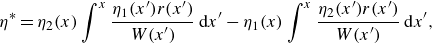 \begin{equation} \eta ^* = \eta _2(x) \int ^x \frac {\eta _1(x') r(x')}{W(x')}\:\textrm{d}x' - \eta _1(x) \int ^x \frac {\eta _2(x') r(x')}{W(x')}\:\textrm{d}x', \end{equation}
where $r(x) = - (1+B) \phi (x, 0)$
is the source term in (A1), and
$r(x) = - (1+B) \phi (x, 0)$
is the source term in (A1), and $W(x) = \eta _1 \eta _2' - \eta _1' \eta _2 = - 2 \sqrt {B}$
is the Wronskian of
$W(x) = \eta _1 \eta _2' - \eta _1' \eta _2 = - 2 \sqrt {B}$
is the Wronskian of $\eta _1$
and
$\eta _1$
and $\eta _2$
. Substituting expressions for
$\eta _2$
. Substituting expressions for $\eta _1, \eta _2, r, W$
into (A4), we have
$\eta _1, \eta _2, r, W$
into (A4), we have
 \begin{equation} \eta * = \frac {1+B}{2\sqrt {B}} \left ( \textrm{e}^{-\sqrt {B} x} \int ^x \phi (x', 0) \textrm{e}^{\sqrt {B} x'} \:\textrm{d}x' - \textrm{e}^{\sqrt {B} x} \int ^x \phi (x', 0) \textrm{e}^{-\sqrt {B} x'} \:\textrm{d}x' \right ). \end{equation}
Therefore, the general solution to (A1) can be given by
 \begin{equation} \eta = c_1 \eta _1 + c_2 \eta _2 + \eta ^*, \end{equation}
where $c_1, c_2$
are arbitrary constants. For
$c_1, c_2$
are arbitrary constants. For $x \gt r$
, we have the boundary conditions specified in (2.12b
), given by
$x \gt r$
, we have the boundary conditions specified in (2.12b
), given by
 \begin{align}& \frac {\textrm{d} \eta }{\textrm{d} x} = - \textrm{i}\Lambda ^{-1} \eta , \quad \text{at } x = r, \end{align}
 \begin{align}& \eta \rightarrow T \textrm{e}^{ \textrm{i}x },\quad \text{as } x \rightarrow +\infty , \end{align}
where the condition at infinity can be further simplified as
 \begin{align}& \frac {\textrm{d} \eta }{\textrm{d} x} = - \textrm{i}\Lambda ^{-1} \eta ,\quad \text{at } x = r, \\[-24pt] \nonumber \end{align}
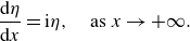 \begin{align}&\,\, \frac {\textrm{d} \eta }{\textrm{d} x} = \textrm{i} \eta ,\quad \text{as } x \rightarrow +\infty . \end{align}
From (A6), we have the form for $\eta$
and
$\eta$
and $\textrm{d} \eta / \textrm{d} x$
:
$\textrm{d} \eta / \textrm{d} x$
:
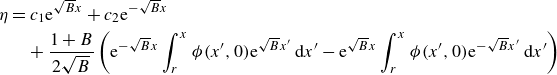 \begin{align} \eta &= c_1 \textrm{e}^{\sqrt {B} x} + c_2 \textrm{e}^{-\sqrt {B} x} \nonumber \\ &\quad + \frac {1+B}{2\sqrt {B}} \left ( \textrm{e}^{-\sqrt {B} x} \int _r^x \phi (x', 0) \textrm{e}^{\sqrt {B} x'} \:\textrm{d}x' - \textrm{e}^{\sqrt {B} x} \int _r^x \phi (x', 0) \textrm{e}^{-\sqrt {B} x'} \:\textrm{d}x' \right ) \end{align}
and
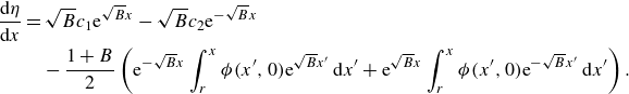 \begin{align} \frac {\textrm{d} \eta }{\textrm{d} x} &= \sqrt {B} c_1 \textrm{e}^{\sqrt {B} x} - \sqrt {B} c_2 \textrm{e}^{-\sqrt {B} x} \nonumber \\ &\quad - \frac {1+B}{2} \left ( \textrm{e}^{-\sqrt {B} x} \int _r^x \phi (x', 0) \textrm{e}^{\sqrt {B} x'} \:\textrm{d}x' + \textrm{e}^{\sqrt {B} x} \int _r^x \phi (x', 0) \textrm{e}^{-\sqrt {B} x'} \:\textrm{d}x' \right ). \end{align}
Substituting (A9) to (A8), we get
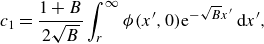 \begin{align}& c_1 = \frac {1+B}{2\sqrt {B}} \int _r^\infty \phi (x', 0) \textrm{e}^{-\sqrt {B} x'} \:\textrm{d}x', \end{align}
 \begin{align}&\qquad\quad c_2 = \frac {\sqrt {B} \Lambda + \textrm{i}}{\sqrt {B} \Lambda - \textrm{i}} \textrm{e}^{2 \sqrt {B} r} c_1. \end{align}
Therefore, if we define the slip parameter:
 \begin{equation} \zeta = \tan ^{-1} \left (\sqrt {B} \Lambda \right ), \end{equation} $c_2$
becomes
$c_2$
becomes
 \begin{align} c_2 &= \frac {\tan \zeta + \textrm{i}}{\tan \zeta - \textrm{i}} \textrm{e}^{2 \sqrt {B} r} c_1 \nonumber \\ &= \textrm{e}^{2\textrm{i} (\frac {\pi }{2} - \zeta )} \textrm{e}^{2 \sqrt {B} r} c_1 \nonumber \\ &= - \frac {1+B}{2\sqrt {B}} \textrm{e}^{-2\textrm{i} \zeta } \textrm{e}^{2 \sqrt {B} r} \int _r^\infty \phi (x', 0) \textrm{e}^{-\sqrt {B} x'} \:\textrm{d}x'. \end{align}
Substituting $c_1, c_2$
to (A9a
):
$c_1, c_2$
to (A9a
):
 \begin{align} \eta &= \frac {1+B}{2\sqrt {B}} \left ( \textrm{e}^{\sqrt {B} x} \int _r^\infty \phi (x', 0) \textrm{e}^{-\sqrt {B} x'} \:\textrm{d}x' - \textrm{e}^{-2\textrm{i} \zeta } \textrm{e}^{2 \sqrt {B} (2r-x)} \int _r^\infty \phi (x', 0) \textrm{e}^{-\sqrt {B} x'} \:\textrm{d}x' \right . \nonumber \\ &\quad \left . + \textrm{e}^{-\sqrt {B} x} \int _r^x \phi (x', 0) \textrm{e}^{\sqrt {B} x'} \:\textrm{d}x' - \textrm{e}^{\sqrt {B} x} \int _r^x \phi (x', 0) \textrm{e}^{-\sqrt {B} x'} \:\textrm{d}x' \right ) \nonumber \\ &= \frac {1+B}{2\sqrt {B}} \left ( \int _r^x \phi (x', 0) \textrm{e}^{\sqrt {B} (x'-x)} \:\textrm{d}x' + \int _x^\infty \phi (x', 0) \textrm{e}^{\sqrt {B} (x-x')} \:\textrm{d}x' \right . \nonumber \\ & \quad \left . - \textrm{e}^{-2\textrm{i} \zeta } \int _r^\infty \phi (x', 0) \textrm{e}^{\sqrt {B} (2r-(x+x'))} \:\textrm{d}x' \right ) \nonumber \\ &= \int _r^\infty \frac {1+B}{2\sqrt {B}} \left ( - \textrm{e}^{-2\textrm{i} \zeta } \textrm{e}^{\sqrt {B} (2r-(x+x'))} +\textrm{e}^{-\sqrt {B} |x-x'|} \right ) \phi (x', 0) \:\textrm{d}x'. \end{align}
For $x \lt -r$
, following the same approach, we have
$x \lt -r$
, following the same approach, we have
 \begin{equation} \eta = \int _{-\infty }^{-r} \frac {1+B}{2\sqrt {B}} \left ( - \textrm{e}^{-2\textrm{i} \zeta } \textrm{e}^{\sqrt {B} (2r+(x+x'))} +\textrm{e}^{-\sqrt {B} |x-x'|} \right ) \phi (x', 0) \:\textrm{d}x'. \end{equation}
Combining (A13) and (A14), we have the solution for $\eta$
in general:
$\eta$
in general:
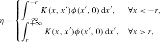 \begin{equation} \eta = \begin{cases} \displaystyle \int ^{- r}_{- \infty } K(x, x') \phi (x', 0) \: \textrm{d} x', & \forall x \lt -r, \\ \displaystyle \int ^{+ \infty }_{r} K(x, x') \phi (x', 0) \: \textrm{d} x', & \forall x \gt r, \end{cases} \end{equation}
where the dynamic kernel $K(x, x')$
is defined as
$K(x, x')$
is defined as
 \begin{equation} K(x, x') = \frac {1+B}{2\sqrt {B}} \left ( -\textrm{e}^{-2\textrm{i}\zeta } \textrm{e}^{\sqrt {B}(2r - |x + x'|)} + \textrm{e}^{-\sqrt {B}|x - x'|} \right ). \end{equation}
Appendix B. Mathematical details in expressing
$\boldsymbol{\phi}\boldsymbol{(x,0)}$

This appendix provides the detailed steps required to derive $\phi (x,0)$
in terms of
$\phi (x,0)$
in terms of $\eta (x)$
, transitioning from (3.11) to (3.12).
$\eta (x)$
, transitioning from (3.11) to (3.12).
Recall (3.11):
 \begin{equation} \psi (u, v) = \frac {1}{2\pi } \int _{-\infty }^{+\infty } g(u') \left (\,\int _{-\infty }^{+\infty } \frac {1}{|\lambda |} \textrm{e}^{|\lambda | v} \,\textrm{e}^{\textrm{i}\lambda (u - u')} \,\textrm{d}\lambda \right ) \textrm{d}u'. \end{equation}
Evaluating at $v=0$
gives
$v=0$
gives
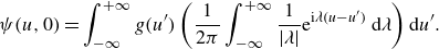 \begin{align} \psi (u, 0) &= \int _{-\infty }^{+\infty } g(u') \left ( \frac {1}{2\pi } \int _{-\infty }^{+\infty } \frac {1}{|\lambda |} \textrm{e}^{\textrm{i}\lambda (u - u')} \,\textrm{d}\lambda \right ) \textrm{d}u'. \end{align}
Recognise that the expression in parentheses is the inverse Fourier transform of $1/|\lambda |$
, namely
$1/|\lambda |$
, namely
 \begin{equation} \frac {1}{2\pi } \int _{-\infty }^{+\infty } \frac {1}{|\lambda |} \,\textrm{e}^{\textrm{i}\lambda (u - u')} \,\textrm{d}\lambda \;=\; \mathcal{F}^{-1}\!\Bigl [\frac {1}{|\lambda |}\Bigr ](u - u') \;=\; -\,\frac {1}{\pi }\,\bigl (\ln |u - u'|\,+\,\gamma \bigr ), \end{equation}
where $\gamma$
is the Euler–Mascheroni constant. Substituting this back into (B2) gives
$\gamma$
is the Euler–Mascheroni constant. Substituting this back into (B2) gives
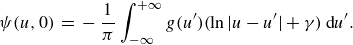 \begin{equation} \psi (u, 0) \;=\; -\,\frac {1}{\pi } \int _{-\infty }^{+\infty } g(u') \bigl (\ln |u - u'| + \gamma \bigr )\,\textrm{d}u'. \end{equation}
Since $\psi (u, v) = \phi (x, y)$
under the conformal mapping, we obtain
$\psi (u, v) = \phi (x, y)$
under the conformal mapping, we obtain
 \begin{equation} \phi (x, 0) \;=\; \psi \bigl (u(x,0),\,v(x,0)\bigr ) \;=\; \psi \bigl (u(x,0),\,0\bigr ). \end{equation}
From the conformal mapping in component form in (3.5), we have
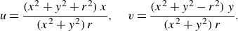 \begin{equation} u = \frac {(x^2 + y^2 + r^2)\,x}{(x^2 + y^2)\,r}, \quad v = \frac {(x^2 + y^2 - r^2)\,y}{(x^2 + y^2)\,r}. \end{equation}
Thus, for $y=0$
,
$y=0$
,
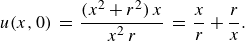 \begin{equation} u(x,0) \;=\; \frac {(x^2 + r^2)\,x}{x^2\,r} \;=\; \frac {x}{r} + \frac {r}{x}. \end{equation}
Next, recall the relation between the boundary function $g(u)$
and the free-surface elevation
$g(u)$
and the free-surface elevation $\eta (x)$
from (3.7):
$\eta (x)$
from (3.7):
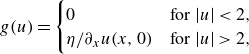 \begin{equation} g(u) = \begin{cases} \displaystyle 0 & \mbox{for } |u| \lt 2, \\ \displaystyle \eta / \partial _x u(x, 0) & \mbox{for } |u| \gt 2, \end{cases} \end{equation}
which implies
 \begin{equation} g(u)\:\textrm{d}u \;=\; \eta (x)\:\textrm{d}x \quad \text{for } |u| \gt 2 \;\;\text{(equivalently, } |x| \gt r\text{).} \end{equation}
Hence, we obtain
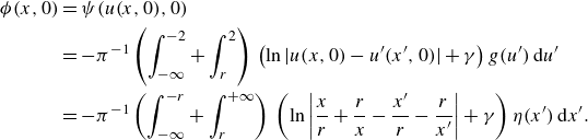 \begin{align} \phi (x, 0) &= \psi (u(x,0), 0) \nonumber \\ &= - \pi ^{-1} \left ( \int _{-\infty }^{-2} + \int _{r}^{2} \right ) \, \left ( \ln {|u(x,0) - u'(x',0)|} + \gamma \right ) g(u') \: \textrm{d} u' \nonumber \\ &= - \pi ^{-1} \left ( \int _{-\infty }^{-r} + \int _{r}^{+\infty } \right ) \, \left ( \ln { \left | \frac {x}{r} + \frac {r}{x} - \frac {x'}{r} - \frac {r}{x'} \right | } + \gamma \right ) \eta (x') \: \textrm{d} x' . \end{align}
Therefore, for $|x|\gt r$
, we arrive at the final expression (3.12):
$|x|\gt r$
, we arrive at the final expression (3.12):
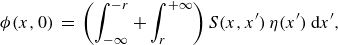 \begin{equation} \phi (x, 0) \;=\; \left ( \int _{-\infty }^{-r} + \int _{r}^{+\infty } \right ) S(x, x')\,\eta (x')\,\textrm{d}x', \end{equation}
where the geometric kernel $S(x, x')$
is given by
$S(x, x')$
is given by
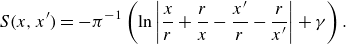 \begin{equation} S (x, x') = - \pi ^{-1} \left ( \ln { \left | \frac {x}{r} + \frac {r}{x} - \frac {x'}{r} - \frac {r}{x'} \right | } + \gamma \right ). \end{equation}
Hence, $\phi (x,0)$
is expressed solely in terms of
$\phi (x,0)$
is expressed solely in terms of $\eta (x)$
through the integral kernel
$\eta (x)$
through the integral kernel $S(x,x')$
.
$S(x,x')$
.
Appendix C. Analytical calculation of
$\boldsymbol{(}\boldsymbol{\mathcal{L}}_{\boldsymbol{\chi}} \boldsymbol{\mathcal{K}} \boldsymbol{-} \boldsymbol{\mathcal{I}}\boldsymbol{)} \textbf{e}^{\boldsymbol{\pm} \textbf{i}\boldsymbol{x}}$

In this appendix, we will analytically calculate $(\mathcal{L}_{\chi } \mathcal{K} - \mathcal{I}) \textrm{e}^{\pm \textrm{i}x}$
that was proposed in (4.11), where
$(\mathcal{L}_{\chi } \mathcal{K} - \mathcal{I}) \textrm{e}^{\pm \textrm{i}x}$
that was proposed in (4.11), where $\chi$
takes the values ‘
$\chi$
takes the values ‘ $e$
’ for even and ‘
$e$
’ for even and ‘ $o$
’ for odd,
$o$
’ for odd, $\mathcal{L}_e$
,
$\mathcal{L}_e$
, $\mathcal{L}_o$
and
$\mathcal{L}_o$
and $\mathcal{K}$
are the integral operators integrated from
$\mathcal{K}$
are the integral operators integrated from $r$
to
$r$
to $\infty$
with kernels
$\infty$
with kernels $L_e$
,
$L_e$
, $L_o$
and
$L_o$
and $K$
given by
$K$
given by
 \begin{align}&\qquad\qquad\quad L_e(x,x') = S(x, x') + S(x, -x') , \end{align}
 \begin{align}&\qquad\qquad\quad L_o(x,x') = S(x, x') - S(x, -x') , \end{align}
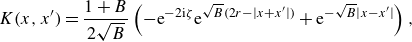 \begin{align}& K(x,x') = \frac {1+B}{2\sqrt {B}} \left ( -\textrm{e}^{-2\textrm{i}\zeta } \textrm{e}^{\sqrt {B}(2r - |x + x'|)} + \textrm{e}^{-\sqrt {B}|x - x'|} \right ) , \end{align}
where
 \begin{equation} S(x, x') = - \pi ^{-1} \left ( \ln \left | \frac {x}{r} + \frac {r}{x} - \frac {x'}{r} - \frac {r}{x'} \right | + \gamma \right ) . \end{equation}
The expression $(\mathcal{L}_{\chi } \mathcal{K} - \mathcal{I}) \textrm{e}^{\pm \textrm{i}x}$
can be written in integral form:
$(\mathcal{L}_{\chi } \mathcal{K} - \mathcal{I}) \textrm{e}^{\pm \textrm{i}x}$
can be written in integral form:
 \begin{align} (\mathcal{L}_{\chi } \mathcal{K} - \mathcal{I}) \textrm{e}^{\pm \textrm{i}x} &= \int _{r}^{+ \infty } L_{\chi }(x, x') \left ( \int _{r}^{+ \infty } K(x', x'') \textrm{e}^{\pm \textrm{i}x''} \: \textrm{d} x'' \right ) \textrm{d} x' - \textrm{e}^{\pm \textrm{i}x} . \end{align}
First, we calculate $\int _{r}^{+ \infty } K(x', x'') \textrm{e}^{\pm \textrm{i}x''} \textrm{d} x''$
:
$\int _{r}^{+ \infty } K(x', x'') \textrm{e}^{\pm \textrm{i}x''} \textrm{d} x''$
:
 \begin{align} \int _{r}^{+ \infty }\!\!\! K(x'\!, x'') \textrm{e}^{\pm \textrm{i}x''} \textrm{d} x'' &= \!\int _{r}^{+ \infty } \frac {1+B}{2\sqrt {B}} \left ( -\textrm{e}^{-2\textrm{i}\zeta } \textrm{e}^{\sqrt {B}(2r - |x' + x''|)} + \textrm{e}^{-\sqrt {B}|x' - x''|} \right ) \textrm{e}^{\pm \textrm{i}x''} \!\textrm{d} x'' \nonumber \\ &= \frac {1}{2 \sqrt {B}} \left [ \!- \!\left(\!\sqrt {B} \pm \textrm{i}\right) \textrm{e}^{-2\textrm{i}\zeta }\! + \left(\!-\sqrt {B} \pm \textrm{i}\right)\! \right ] \textrm{e}^{(\sqrt {B} \pm \textrm{i}) r} \textrm{e}^{- \sqrt {B} x'} \!\! + \textrm{e}^{\pm \textrm{i}x'} . \end{align}
Substituting (C3) into (C2), we have
 \begin{equation} (\mathcal{L}_{\chi } \mathcal{K} - \mathcal{I}) \textrm{e}^{\pm \textrm{i}x} = - \textrm{e}^{\pm \textrm{i}x} + \frac {1}{2 \sqrt {B}} \left [\! - \!\left(\!\sqrt {B} \pm \textrm{i}\right) \textrm{e}^{-2\textrm{i}\zeta } \!+ \left(\!-\sqrt {B} \pm \textrm{i}\right)\! \right ] \textrm{e}^{(\sqrt {B} \pm \textrm{i}) r} I_{1, \chi }\! +\! I_{2, \chi , \pm } , \end{equation}
where
 \begin{align}& I_{1, \chi } = \int _{r}^{+ \infty } L_{\chi }(x, x') \textrm{e}^{- \sqrt {B} x'} \textrm{d} x' , \end{align}
 \begin{align}& I_{2, \chi , \pm } = \int _{r}^{+ \infty } L_{\chi }(x, x') \textrm{e}^{\pm \textrm{i}x'} \textrm{d} x' . \end{align}
Since $L_e = S(x, x') + S(x, -x')$
and
$L_e = S(x, x') + S(x, -x')$
and $L_e = S(x, x') - S(x, -x')$
, first we calculate
$L_e = S(x, x') - S(x, -x')$
, first we calculate
 \begin{align} \int _{r}^{+ \infty } S(x, x') \textrm{e}^{- \sqrt {B} x'} \textrm{d} x' &= - \pi ^{-1} \int _{r}^{+ \infty } \left ( \ln { \left | \frac {x}{r} + \frac {r}{x} - \frac {x'}{r} - \frac {r}{x'} \right | } + \gamma \right ) \textrm{e}^{- \sqrt {B} x'} \textrm{d} x' \nonumber \\ &= \frac {1}{\pi \sqrt {B}} \left ( \textrm{e}^{-\frac {\sqrt {B} r^2}{x}} \operatorname {Ei}\left ( -\frac {\sqrt {B} r (x-r)}{x} \right ) \right . \nonumber \\ &\quad + \textrm{e}^{-\sqrt {B} x} \operatorname {Ei}(\sqrt {B}(x-r)) \nonumber \\ &\quad \left . -\operatorname {Ei}(-\sqrt {B} r) - \ln { \left | \frac {x}{r} + \frac {r}{x} - 2 \right | } \textrm{e}^{-\sqrt {B} r} - \gamma \textrm{e}^{-\sqrt {B} r} \vphantom{\frac {\sqrt {B} r (x-r)}{x}}\right ) . \end{align}
Since $S(x, -x') = S(-x, x')$
, we have
$S(x, -x') = S(-x, x')$
, we have
 \begin{align} \int _{r}^{+ \infty } S(x, -x') \textrm{e}^{- \sqrt {B} x'} \textrm{d} x' &= \int _{r}^{+ \infty } S(-x, x') \textrm{e}^{- \sqrt {B} x'} \textrm{d} x' \nonumber \\ &=\frac {1}{\pi \sqrt {B}} \left ( \textrm{e}^{\frac {\sqrt {B} r^2}{x}} \operatorname {Ei}\left ( -\frac {\sqrt {B} r (x+r)}{x} \right ) \right . \nonumber \\ &\quad + \textrm{e}^{\sqrt {B} x} \operatorname {Ei}(-\sqrt {B}(x+r)) \nonumber \\ & \quad \left . -\operatorname {Ei}(-\sqrt {B} r) - \ln { \left | \frac {x}{r} + \frac {r}{x} + 2 \right | } \textrm{e}^{-\sqrt {B} r} - \gamma \textrm{e}^{-\sqrt {B} r} \vphantom{\frac {\sqrt {B} r (x-r)}{x}}\right ) . \end{align}
Now, we calculate $I_1$
:
$I_1$
:
 \begin{align} I_{1, e} &= \int _{r}^{+ \infty } L_{e}(x, x') \textrm{e}^{- \sqrt {B} x'} \textrm{d} x' \nonumber \\ &= \int _{r}^{+ \infty } S(x, x') \textrm{e}^{- \sqrt {B} x'} \textrm{d} x' + \int _{r}^{+ \infty } S(x, -x') \textrm{e}^{- \sqrt {B} x'} \textrm{d} x' \nonumber \\ &= \frac {1}{\pi \sqrt {B}} \left ( \textrm{e}^{-\frac {\sqrt {B} r^2}{x}} \operatorname {Ei}\left ( -\frac {\sqrt {B} r (x-r)}{x} \right ) + \textrm{e}^{\frac {\sqrt {B} r^2}{x}} \operatorname {Ei}\left ( -\frac {\sqrt {B} r (x+r)}{x} \right ) \right .\nonumber \\ &\quad + \textrm{e}^{-\sqrt {B} x} \operatorname {Ei}(\sqrt {B}(x-r)) + \textrm{e}^{\sqrt {B} x} \operatorname {Ei}(-\sqrt {B}(x+r)) \nonumber \\ &\quad \left . - 2 \operatorname {Ei}(-\sqrt {B} r) - 2 \ln { \left ( \frac {x}{r} - \frac {r}{x} \right ) } \textrm{e}^{-\sqrt {B} r} - 2 \gamma \textrm{e}^{-\sqrt {B} r} \right ) , \end{align}
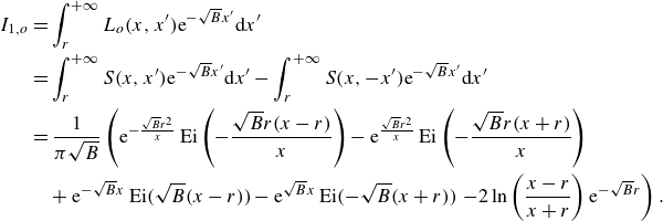 \begin{align} I_{1, o} &= \int _{r}^{+ \infty } L_{o}(x, x') \textrm{e}^{- \sqrt {B} x'} \textrm{d} x' \nonumber \\ &= \int _{r}^{+ \infty } S(x, x') \textrm{e}^{- \sqrt {B} x'} \textrm{d} x' - \int _{r}^{+ \infty } S(x, -x') \textrm{e}^{- \sqrt {B} x'} \textrm{d} x' \nonumber \\ &= \frac {1}{\pi \sqrt {B}} \left ( \textrm{e}^{-\frac {\sqrt {B} r^2}{x}} \operatorname {Ei}\left ( -\frac {\sqrt {B} r (x-r)}{x} \right ) - \textrm{e}^{\frac {\sqrt {B} r^2}{x}} \operatorname {Ei}\left ( -\frac {\sqrt {B} r (x+r)}{x} \right ) \right . \nonumber \\ &\quad + \textrm{e}^{-\sqrt {B} x} \operatorname {Ei}(\sqrt {B}(x-r)) - \textrm{e}^{\sqrt {B} x} \operatorname {Ei}(-\sqrt {B}(x+r)) \left . - 2 \ln { \left ( \frac {x - r}{x + r} \right ) }\, \textrm{e}^{-\sqrt {B} r} \right ) . \end{align}
Some care is needed in the calculation of $I_2$
. Since
$I_2$
. Since $\textrm{e}^{\pm \textrm{i}x}$
is
$\textrm{e}^{\pm \textrm{i}x}$
is $O(1)$
and
$O(1)$
and $L_\chi$
is
$L_\chi$
is $O(\ln x)$
at
$O(\ln x)$
at $x \rightarrow \infty$
,
$x \rightarrow \infty$
, $I_2$
is not converged in the range
$I_2$
is not converged in the range $[r, \infty ]$
. Some mathematical technique is used to calculate the principal value of
$[r, \infty ]$
. Some mathematical technique is used to calculate the principal value of $I_2$
, as shown below:
$I_2$
, as shown below:
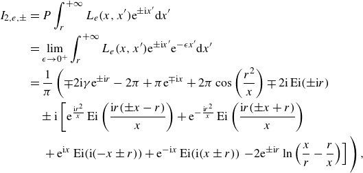 \begin{align} I_{2, e, \pm } &= P \int _{r}^{+ \infty } L_{e}(x, x') \textrm{e}^{\pm \textrm{i}x'} \textrm{d} x' \nonumber \\ &= \lim _{\epsilon \rightarrow 0^+} \int _{r}^{+ \infty } L_{e}(x, x') \textrm{e}^{\pm \textrm{i}x'} \textrm{e}^{- \epsilon x'} \textrm{d} x' \nonumber \\ &=\frac {1}{\pi } \left ( \mp 2\textrm{i}\gamma \textrm{e}^{\pm \textrm{i}r} - 2\pi + \pi \textrm{e}^{\mp \textrm{i}x} + 2\pi \cos \left (\frac {r^2}{x}\right ) \mp 2\textrm{i}\operatorname {Ei}(\pm \textrm{i}r) \right . \nonumber \\ &\quad \pm \textrm{i}\left [ \textrm{e}^{\frac {\textrm{i}r^2}{x}} \operatorname {Ei}\left (\frac {\textrm{i}r(\pm x-r)}{x}\right ) + \textrm{e}^{-\frac {\textrm{i}r^2}{x}} \operatorname {Ei}\left (\frac {\textrm{i}r(\pm x+r)}{x}\right ) \right . \nonumber \\ &\quad \ + \textrm{e}^{\textrm{i}x} \operatorname {Ei}(\textrm{i}(-x\pm r)) + \textrm{e}^{-\textrm{i}x} \operatorname {Ei}(\textrm{i}(x\pm r)) \left . \left . - 2\textrm{e}^{\pm \textrm{i}r} \ln \left (\frac {x}{r}-\frac {r}{x}\right )\right ] \vphantom{\frac {\sqrt {B} r (x-r)}{x}} \right ) , \end{align}
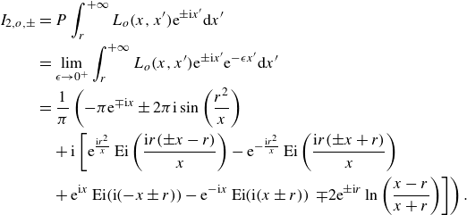 \begin{align} I_{2, o, \pm } &= P \int _{r}^{+ \infty } L_{o}(x, x') \textrm{e}^{\pm \textrm{i}x'} \textrm{d} x' \nonumber \\ &= \lim _{\epsilon \rightarrow 0^+} \int _{r}^{+ \infty } L_{o}(x, x') \textrm{e}^{\pm \textrm{i}x'} \textrm{e}^{- \epsilon x'} \textrm{d} x' \nonumber \\ &= \frac {1}{\pi } \left ( - \pi \textrm{e}^{\mp \textrm{i}x} \pm 2\pi \textrm{i}\sin \left (\frac {r^2}{x}\right ) \right .\nonumber \\ &\quad + \textrm{i}\left [ \textrm{e}^{\frac {\textrm{i}r^2}{x}} \operatorname {Ei}\left (\frac {\textrm{i}r(\pm x-r)}{x}\right ) - \textrm{e}^{-\frac {\textrm{i}r^2}{x}} \operatorname {Ei}\left (\frac {\textrm{i}r(\pm x+r)}{x}\right ) \right .\nonumber \\ &\quad + \textrm{e}^{\textrm{i}x} \operatorname {Ei}(\textrm{i}(-x\pm r)) - \textrm{e}^{- \textrm{i}x} \operatorname {Ei}(\textrm{i}(x\pm r)) \left . \left . \mp 2\textrm{e}^{\pm \textrm{i}r} \ln \left (\frac {x-r}{x+r}\right )\right ] \right ) . \\[9pt] \nonumber \end{align}
Now, we have the analytical expression for $(\mathcal{L}_{\chi } \mathcal{K} - \mathcal{I}) \textrm{e}^{\pm \textrm{i}x}$
, recalling (C4):
$(\mathcal{L}_{\chi } \mathcal{K} - \mathcal{I}) \textrm{e}^{\pm \textrm{i}x}$
, recalling (C4):
 \begin{equation} (\mathcal{L}_{\chi } \mathcal{K} - \mathcal{I}) \textrm{e}^{\pm \textrm{i}x} = - \textrm{e}^{\pm \textrm{i}x} + \frac {1}{2 \sqrt {B}} \left [ \!- (\sqrt {B} \pm \textrm{i}) \textrm{e}^{-2\textrm{i}\zeta } \!+ (-\sqrt {B} \pm \textrm{i}) \right ] \textrm{e}^{(\sqrt {B} \pm \textrm{i}) r} I_{1, \chi }\! + I_{2, \chi , \pm } , \end{equation}

Appendix D. Analytical solution for T, R in scattering by an infinitesimal barrier
In this appendix, we will solve integral equations proposed in (7.5):
 \begin{equation} h_{\chi , \pm } = \mathcal{L}_{\chi } \mathcal{K} h_{\chi ,\pm } + g_{\chi , \pm } , \end{equation}
where $\chi$
takes the values ‘
$\chi$
takes the values ‘ $e$
’ for even and ‘
$e$
’ for even and ‘ $o$
’ for odd,
$o$
’ for odd, $\mathcal{L}_e$
,
$\mathcal{L}_e$
, $\mathcal{L}_o$
and
$\mathcal{L}_o$
and $\mathcal{K}$
are the integral operators integrate from
$\mathcal{K}$
are the integral operators integrate from $0$
to
$0$
to $\infty$
with kernels
$\infty$
with kernels $L_e$
,
$L_e$
, $L_o$
and
$L_o$
and $K$
given by
$K$
given by
 \begin{align}&\quad L_e(x,x') = - \pi ^{-1} \left ( \ln \left | x - x' \right | + \ln \left ( x + x' \right ) + 2 \gamma \right ) , \end{align}
 \begin{align}&\qquad L_o(x,x') = - \pi ^{-1} \left ( \ln \left | x - x' \right | - \ln \left ( x + x' \right ) \right ) , \end{align}
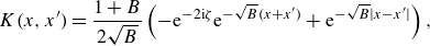 \begin{align}& K(x,x') = \frac {1+B}{2\sqrt {B}} \left ( -\textrm{e}^{-2\textrm{i}\zeta } \textrm{e}^{- \sqrt {B} (x + x')} + \textrm{e}^{-\sqrt {B}|x - x'|} \right ) , \end{align}
and $g_{\chi , \pm } = (\mathcal{L}_{\chi } \mathcal{K} - \mathcal{I}) \textrm{e}^{\pm \textrm{i}x}$
can be calculated analytically through similar methods as in Appendix C:
$g_{\chi , \pm } = (\mathcal{L}_{\chi } \mathcal{K} - \mathcal{I}) \textrm{e}^{\pm \textrm{i}x}$
can be calculated analytically through similar methods as in Appendix C:
 \begin{align} g_{e, \pm } &= (\mathcal{L}_{e} \mathcal{K} - \mathcal{I}) \textrm{e}^{\pm \textrm{i}x} \nonumber \\ &=\int _{0}^{+ \infty } L_{e}(x, x') \left ( \int _{0}^{+ \infty } K(x', x'') \textrm{e}^{\pm \textrm{i}x''} \textrm{d} x'' \right ) \textrm{d} x' - \textrm{e}^{\pm \textrm{i}x} \nonumber \\ &= \mp 2 \textrm{i}\sin x \pm \frac {\textrm{i}}{\pi } \left [ \textrm{e}^{\textrm{i}x} \operatorname {Ei}(- \textrm{i}x) + \textrm{e}^{- \textrm{i}x} \operatorname {Ei}(\textrm{i}x) - 2 (\gamma + \ln |x|) \right ] \nonumber \\ &\quad + \frac {- (\sqrt {B} \pm \textrm{i}) \textrm{e}^{- 2 \textrm{i}\zeta } + (- \sqrt {B} \pm \textrm{i})}{2 \pi B} \nonumber \\ &\quad \times \left [ \textrm{e}^{\sqrt {B} x} \operatorname {Ei}(- \sqrt {B} x) + \textrm{e}^{- \sqrt {B} x} \operatorname {Ei}(\sqrt {B} x) - 2 (\gamma + \ln |x|) \right ], \end{align}
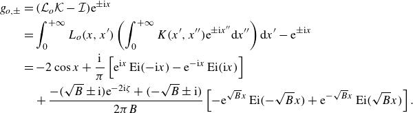 \begin{align} g_{o, \pm } &= (\mathcal{L}_{o} \mathcal{K} - \mathcal{I}) \textrm{e}^{\pm \textrm{i}x} \nonumber \\ &=\int _{0}^{+ \infty } L_{o}(x, x') \left ( \int _{0}^{+ \infty } K(x', x'') \textrm{e}^{\pm \textrm{i}x''} \textrm{d} x'' \right ) \textrm{d} x' - \textrm{e}^{\pm \textrm{i}x} \nonumber \\ &= - 2 \cos x + \frac {\textrm{i}}{\pi } \left [ \textrm{e}^{\textrm{i}x} \operatorname {Ei}(- \textrm{i}x) - \textrm{e}^{- \textrm{i}x} \operatorname {Ei}(\textrm{i}x) \right ] \nonumber \\ &\quad + \frac {- (\sqrt {B} \pm \textrm{i}) \textrm{e}^{- 2 \textrm{i}\zeta } + (- \sqrt {B} \pm \textrm{i})}{2 \pi B} \left [ - \textrm{e}^{\sqrt {B} x} \operatorname {Ei}(- \sqrt {B} x) + \textrm{e}^{- \sqrt {B} x} \operatorname {Ei}(\sqrt {B} x) \right ]. \end{align}
First, we solve for $h_e$
. We apply a Fourier cosine transform (FCT)
$h_e$
. We apply a Fourier cosine transform (FCT)
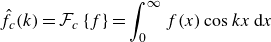 \begin{equation} \hat {f}_c(k) = \mathcal{F}_c\left \{ f \right \} = \int _0^\infty f(x) \cos kx \: \textrm{d} x \end{equation}
to (D1), and we obtain
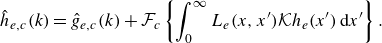 \begin{equation} \hat {h}_{e,c}(k) = \hat {g}_{e,c}(k) + \mathcal{F}_c\left \{\int _0^\infty L_e(x, x') \mathcal{K} h_e(x') \,\textrm{d}x' \right \} . \end{equation}
The second term on the right side can be expanded as
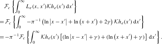 \begin{align} &\quad \mathcal{F}_c\left \{\int _0^\infty L_e(x, x')\mathcal{K} h_e(x') \: \textrm{d} x' \right \} \nonumber \\ &= \mathcal{F}_c\left \{ \int _0^\infty - \pi ^{-1} \left ( \ln \left | x - x' \right | + \ln \left ( x + x' \right ) + 2 \gamma \right ) \mathcal{K} h_e(x') \: \textrm{d} x' \right \} \nonumber \\ &= - \pi ^{-1} \mathcal{F}_c\left \{ \int _0^\infty \mathcal{K} h_e(x') \left [ ( \ln \left | x - x' \right | + \gamma ) + ( \ln \left ( x + x' \right ) + \gamma ) \right ] \: \textrm{d} x'\right \} . \end{align}
For FCT, we have the convolution theorem:
 \begin{equation} 2 \mathcal{F}_c\left \{ f \right \} \mathcal{F}_c\left \{ g \right \} = \mathcal{F}_c\left \{ \int _0^\infty f(x') \left [ g(x + x') + g(|x - x'|) \right ] \: \textrm{d} x' \right \}. \end{equation}
Therefore,
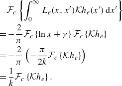 \begin{align} &\quad \mathcal{F}_c\left \{\int _0^\infty L_e(x, x') \mathcal{K} h_e(x') \: \textrm{d} x' \right \} \nonumber \\ &= - \frac {2}{\pi } \mathcal{F}_c\left \{ \ln x + \gamma \right \} \mathcal{F}_c\left \{ \mathcal{K} h_e \right \} \nonumber \\ &= - \frac {2}{\pi } \left ( - \frac {\pi }{2k} \mathcal{F}_c\left \{ \mathcal{K} h_e \right \} \right ) \nonumber \\ &= \frac {1}{k} \mathcal{F}_c\left \{ \mathcal{K} h_e \right \} . \end{align}
The FCT of $\mathcal{K} h_e$
can be calculated by
$\mathcal{K} h_e$
can be calculated by
 \begin{align} &\mathcal{F}_c\left \{ \mathcal{K} h_e \right \} = \mathcal{F}_c\left \{ \int _0^\infty \frac {1+B}{2\sqrt {B}} \left ( -\textrm{e}^{-2\textrm{i}\zeta } \textrm{e}^{- \sqrt {B} (x + x')} + \textrm{e}^{-\sqrt {B}|x - x'|} \right ) h_e(x') \: \textrm{d} x' \right \} \nonumber \\ &= \frac {1+B}{2\sqrt {B}} \left ( \mathcal{F}_c\left \{ \int _0^\infty \left ( \textrm{e}^{- \sqrt {B} (x + x')} + \textrm{e}^{-\sqrt {B}|x - x'|} \right ) h_e(x') \: \textrm{d} x' \right \} \right .\nonumber \\ &\quad \left . - (1 + \textrm{e}^{-2 \textrm{i}\zeta }) \mathcal{F}_c\left \{ \int _0^\infty \textrm{e}^{- \sqrt {B} (x + x')} h_e(x') \: \textrm{d} x' \right \} \right ) \nonumber \\ &= \frac {1+B}{2\sqrt {B}} \left ( 2 \mathcal{F}_c\left \{ \textrm{e}^{- \sqrt {B} x} \right \} \hat {h}_{e,c}(k) - (1 + \textrm{e}^{-2 \textrm{i}\zeta }) \mathcal{F}_c\left \{ \textrm{e}^{- \sqrt {B} x} \right \} \int _0^\infty \textrm{e}^{- \sqrt {B} x'} h_e(x') \: \textrm{d} x' \right ) \nonumber \\ &= \frac {1+B}{2\sqrt {B}} \left ( 2 \frac {\sqrt {B}}{B + k^2} \hat {h}_{e,c}(k) - (1 + \textrm{e}^{-2 \textrm{i}\zeta }) \frac {\sqrt {B}}{B + k^2} \int _0^\infty \textrm{e}^{- \sqrt {B} x'} h_e(x') \: \textrm{d} x' \right ) \nonumber \\ &= \frac {1+B}{B+k^2} \left ( \hat {h}_{e,c}(k) - \frac {1 + \textrm{e}^{-2 \textrm{i}\zeta }}{2} \int _0^\infty \textrm{e}^{- \sqrt {B} x'} h_e(x') \: \textrm{d} x' \right ) . \end{align}
Substituting all these back into (D6), we have
 \begin{equation} \hat {h}_{e,c}(k) = \hat {g}_{e,c}(k) + \frac {1+B}{k(B+k^2)} \left ( \hat {h}_{e,c}(k) - \frac {1 + \textrm{e}^{-2 \textrm{i}\zeta }}{2} \int _0^\infty \textrm{e}^{- \sqrt {B} x'} h_e(x') \: \textrm{d} x' \right ) . \end{equation}
We want to express the integral on the right side in the $k$
-domain, we can write
$k$
-domain, we can write $h$
with an inverse FCT:
$h$
with an inverse FCT:
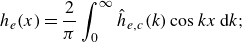 \begin{equation} h_e(x) = \frac {2}{\pi } \int _0^\infty \hat {h}_{e,c}(k) \cos kx \: \textrm{d} k; \end{equation}
therefore, the integral in (D11) can be written as
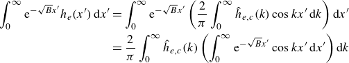 \begin{align*} \int _0^\infty \textrm{e}^{- \sqrt {B} x'} h_e(x') \: \textrm{d} x' &= \int _0^\infty \textrm{e}^{- \sqrt {B} x'} \left ( \frac {2}{\pi } \int _0^\infty \hat {h}_{e,c}(k) \cos kx' \: \textrm{d} k \right ) \textrm{d} x' \nonumber \\&= \frac {2}{\pi } \int _0^\infty \hat {h}_{e,c}(k) \left ( \int _0^\infty \textrm{e}^{- \sqrt {B} x'} \cos kx' \: \textrm{d} x' \right ) \textrm{d} k \end{align*}
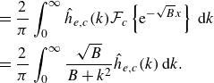 \begin{align} &= \frac {2}{\pi } \int _0^\infty \hat {h}_{e,c}(k) \mathcal{F}_c\left \{ \textrm{e}^{- \sqrt {B} x} \right \} \: \textrm{d} k \nonumber \\&= \frac {2}{\pi } \int _0^\infty \frac {\sqrt {B}}{B+k^2} \hat {h}_{e,c}(k) \: \textrm{d} k . \end{align}
Substituting back to (D11), we obtain
 \begin{equation} \hat {h}_{e,c}(k) = \hat {g}_{e,c}(k) + \frac {1+B}{k(B+k^2)} \left ( \hat {h}_{e,c}(k) - \frac {1 + \textrm{e}^{-2 \textrm{i}\zeta }}{\pi } \int _0^\infty \frac {\sqrt {B}}{B+k^2} \hat {h}_{e,c}(k) \: \textrm{d} k \right ) , \end{equation}
which can be rearranged as
 \begin{equation} \hat {h}_{e,c}(k) = c \delta (k-1) + k (B+k^2) \hat {w}_c(k) \hat {g}_{e,c}(k) - \alpha \hat {w}_c(k) \int _0^\infty \frac {\hat {h}_{e,c}(k)}{B+k^2} \: \textrm{d} k , \end{equation}
where $c$
is a constant to be determined, and
$c$
is a constant to be determined, and
 \begin{align}&\quad \alpha = \pi ^{-1} \sqrt {B} (1+B) (1 + \textrm{e}^{-2 \textrm{i}\zeta }) , \end{align}
 \begin{align}& \hat {w}_c(k) = (k-1)^{-1}(k^2 + k + 1 + B)^{-1} . \end{align}
(D15a
) can be solved by dividing $B + k^2$
on both sides and integrating with respect to
$B + k^2$
on both sides and integrating with respect to $k$
from
$k$
from $0$
to
$0$
to $\infty$
:
$\infty$
:
 \begin{equation} \int _0^\infty \frac {\hat {h}_{e,c}(k)}{B+k^2} \: \textrm{d} k = \frac {c}{B+1} + \int _0^\infty k \hat {w}_c(k) \hat {g}_{e,c}(k) \: \textrm{d} k - \alpha \int _0^\infty \frac {\hat {w}_c(k)}{B+k^2} \: \textrm{d} k \cdot \int _0^\infty \frac {\hat {h}_{e,c}(k)}{B+k^2} \: \textrm{d} k . \end{equation}
Rearranging, we have
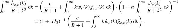 \begin{align} \int _0^\infty \frac {\hat {h}_{e,c}(k)}{B+k^2} \: \textrm{d} k &= \left ( \frac {c}{B+1} + \int _0^\infty k \hat {w}_c(k) \hat {g}_{e,c}(k) \: \textrm{d} k \right ) \cdot \left ( 1 + \alpha \int _0^\infty \frac {\hat {w}_c(k)}{B+k^2} \: \textrm{d} k \right )^{-1} \nonumber \\ &= \left ( 1 + \alpha I_3 \right )^{-1} \left ( \frac {c}{B+1} + \int _0^\infty k \hat {w}_c(k) \hat {g}_{e,c}(k) \: \textrm{d} k \right ) , \end{align}
where
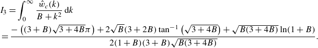 \begin{align} &I_3 = \int _0^\infty \frac {\hat {w}_c(k)}{B+k^2} \: \textrm{d} k \nonumber \\ &= \frac {-\left ((3 + B) \sqrt {3 + 4B} \pi \right ) + 2 \sqrt {B} (3 + 2 B) \tan ^{-1}\left (\sqrt {3 + 4 B}\right ) + \sqrt {B (3 + 4 B)} \ln (1 + B)}{2 (1 + B) (3 + B) \sqrt {B (3 + 4 B)}} . \end{align}
Thus,
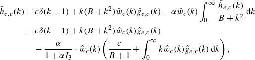 \begin{align} \hat {h}_{e,c}(k) &= c \delta (k-1) + k (B+k^2) \hat {w}_c(k) \hat {g}_{e,c}(k) - \alpha \hat {w}_c(k) \int _0^\infty \frac {\hat {h}_{e,c}(k)}{B+k^2} \: \textrm{d} k \nonumber \\ &= c \delta (k-1) + k (B+k^2) \hat {w}_c(k) \hat {g}_{e,c}(k) \nonumber \\ &\quad - \frac {\alpha }{1 + \alpha I_3} \cdot \hat {w}_c(k) \left ( \frac {c}{B+1} + \int _0^\infty k \hat {w}_c(k) \hat {g}_{e,c}(k) \: \textrm{d} k \right ) , \end{align}
where $\hat {g}_{e,c}$
can be calculated by
$\hat {g}_{e,c}$
can be calculated by
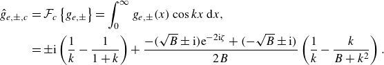 \begin{align} \hat {g}_{e,\pm ,c} &= \mathcal{F}_c\left \{ g_{e, \pm } \right \} = \int _0^\infty g_{e,\pm }(x) \cos kx \: \textrm{d} x , \nonumber \\ &= \pm \textrm{i}\left ( \frac {1}{k} - \frac {1}{1 + k} \right ) + \frac { - (\sqrt {B} \pm \textrm{i}) \textrm{e}^{-2\textrm{i}\zeta } + (-\sqrt {B} \pm \textrm{i}) }{2 B} \left ( \frac {1}{k} - \frac {k}{B + k^2} \right ) . \end{align}
Notice that on the positive $k$
-axis, only the singularity terms in
$k$
-axis, only the singularity terms in $h_c$
correspond to the terms in
$h_c$
correspond to the terms in $h$
that propagate as
$h$
that propagate as $x \rightarrow \infty$
. In this instance, there are two singularity terms on the positive
$x \rightarrow \infty$
. In this instance, there are two singularity terms on the positive $k$
-axis in
$k$
-axis in $h_{e,c}$
:
$h_{e,c}$
: $(k-1)^{-1}$
and
$(k-1)^{-1}$
and $\delta (k-1)$
, which correspond to
$\delta (k-1)$
, which correspond to $\sin x$
and
$\sin x$
and $\cos x$
, respectively, at
$\cos x$
, respectively, at $x \rightarrow \infty$
in
$x \rightarrow \infty$
in $h_e$
. Since the equations for calculating
$h_e$
. Since the equations for calculating $T$
and
$T$
and $R$
((4.14a
) and (4.14b
)) only require the ratio
$R$
((4.14a
) and (4.14b
)) only require the ratio $h_{e, -}/h_{e, +}$
, it is sufficient to calculate this ratio using the coefficients of the
$h_{e, -}/h_{e, +}$
, it is sufficient to calculate this ratio using the coefficients of the $(k-1)^{-1}$
terms for
$(k-1)^{-1}$
terms for $\hat {h}_{e,-,c}$
and
$\hat {h}_{e,-,c}$
and $\hat {h}_{e,+,c}$
. It can also be shown (albeit through another lengthy derivation) that the coefficient of
$\hat {h}_{e,+,c}$
. It can also be shown (albeit through another lengthy derivation) that the coefficient of $\delta (k-1)$
is equal to the coefficient of
$\delta (k-1)$
is equal to the coefficient of $(k-1)^{-1}$
; we omit that proof for brevity. By substituting the expressions for
$(k-1)^{-1}$
; we omit that proof for brevity. By substituting the expressions for $\alpha$
,
$\alpha$
, $\hat {w}_{c}$
and
$\hat {w}_{c}$
and $\hat {g}_{e,c}$
into (D18) and extracting the coefficients of the
$\hat {g}_{e,c}$
into (D18) and extracting the coefficients of the $(k-1)^{-1}$
terms, we obtain the following expression for
$(k-1)^{-1}$
terms, we obtain the following expression for $C_e$
:
$C_e$
:
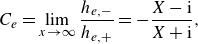 \begin{equation} C_e = \lim _{x\rightarrow \infty }\frac {h_{e, -}}{h_{e, +}} = - \frac {X - \textrm{i}}{X + \textrm{i}} , \end{equation}
where
 \begin{equation} X = \frac {1}{\pi } \left ( \frac {3+2B}{\sqrt {3+4B}} \tan ^{-1} \sqrt {3+4B} + \frac {1}{2} \ln (1+B) \right ) + \textrm{i}\frac {(3+B) \tan \zeta }{2\sqrt {B}} . \end{equation}
Similarly, $h_o$
can be analysed by applying a Fourier sine transform (FST) as follows:
$h_o$
can be analysed by applying a Fourier sine transform (FST) as follows:
 \begin{equation} \hat {f}_s(k) = \mathcal{F}_s\left \{ f \right \} = \int _0^\infty f(x) \sin kx \: \textrm{d} x , \end{equation}
to (D1). The approach remains consistent, albeit the convolution theorem for FST differs:
 \begin{equation} 2 \mathcal{F}_s\left \{ f \right \} \mathcal{F}_c\left \{ g \right \} = \mathcal{F}_s\left \{ \int _0^\infty f(x') \left [ g(|x - x'|) - g(x + x') \right ] \: \textrm{d} x' \right \}. \end{equation}
The details are omitted. The calculated expression for $C_o$
is
$C_o$
is
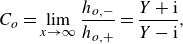 \begin{equation} C_o = \lim _{x\rightarrow \infty } \frac {h_{o, -}}{h_{o, +}} = \frac {Y + \textrm{i}}{Y - \textrm{i}} , \end{equation}
where
 \begin{equation} Y = \frac {1}{\pi } \left ( \frac {3+6B+2B^2}{\sqrt {3+4B}} \tan ^{-1} \sqrt {3+4B} - \frac {1}{2} \ln (1+B) \right ) - \textrm{i}\frac {(3+B) \sqrt {B}}{2 \tan \zeta } . \end{equation}
From (4.14a
) and (4.14b
), we have the theoretical results for the transmission $T$
and the reflection
$T$
and the reflection $R$
coefficients of the infinitesimal barrier (
$R$
coefficients of the infinitesimal barrier ( $r \ll 1$
) case:
$r \ll 1$
) case:
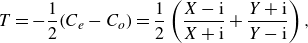 \begin{align} T &= -\frac {1}{2} (C_e - C_o) = \frac {1}{2} \left ( \frac {X-\textrm{i}}{X+\textrm{i}} + \frac {Y+\textrm{i}}{Y-\textrm{i}} \right ) , \end{align}
 \begin{align} R &= -\frac {1}{2} (C_e + C_o) = \frac {1}{2} \left ( \frac {X-\textrm{i}}{X+\textrm{i}} - \frac {Y+\textrm{i}}{Y-\textrm{i}} \right ) . \end{align}
These expressions are consistent with expressions from Hocking (Reference Hocking1987b ), see Appendix E for details.
Appendix E. Expressions for T, R in infinitesimal barrier case (Hocking Reference Hocking1987b )
Hocking (Reference Hocking1987b
) considered scattering of capillary–gravity waves from an infinitesimally thin barrier of a finite immersed depth. In the limit of a zero depth, an analytical results followed from Hocking (Reference Hocking1987b
) for the transmission and reflection coefficients, $T$
and
$T$
and $R$
. Here, we show that these results agree with our analytical solutions of
$R$
. Here, we show that these results agree with our analytical solutions of $T$
and
$T$
and $R$
, (7.8), derived for a cylindrical barrier of a zero cross-section.
$R$
, (7.8), derived for a cylindrical barrier of a zero cross-section.
The coefficients $T$
and
$T$
and $R$
by Hocking (Reference Hocking1987b
) were derived in terms of the inverse Bond number
$R$
by Hocking (Reference Hocking1987b
) were derived in terms of the inverse Bond number
 \begin{equation} K = \frac {\sigma k^2}{\rho g}, \end{equation}
and a dimensionless slip coefficient
 \begin{equation} \lambda = \sqrt {\frac {k}{g}} \Lambda '. \end{equation}
In terms of $K$
and
$K$
and $\lambda$
, the coefficients were given as
$\lambda$
, the coefficients were given as
 \begin{align} T &= \frac {\textrm{i}(\alpha - \beta )}{(1-\textrm{i}\alpha ) (1-\textrm{i}\beta )}, \end{align}
 \begin{align} R &= \frac {1 + \alpha \beta }{(1-\textrm{i}\alpha ) (1-\textrm{i}\beta )}, \end{align}
where
 \begin{align} \alpha &= \frac {2 K}{(1+3K)(J_1(K)-\textrm{i}\lambda (1+K)^{-1/2})}, \end{align}
 \begin{align} \beta &= J_2(K)+\textrm{i}(1+3K)(1+K)^{1/2}/2K\lambda , \end{align}
and
 \begin{align}& J_1(K) = \frac {2K}{\pi (1+3K)} \left \{ \frac {1}{2}\ln \frac {K+1}{K} + \frac {3K+2}{K^{1/2}(3K+4)^{1/2}}\tan ^{-1} \left ( \frac {3K+4}{K} \right )^{1/2} \right \} , \end{align}
 \begin{align}&\quad J_2(K) = \frac {1}{\pi K} \left \{ -\frac {K}{2} \ln \frac {K+1}{K} + \frac {3K^2+6K+2}{K^{1/2}(3K+4)^{1/2}}\tan ^{-1} \left ( \frac {3K+4}{K} \right )^{1/2} \right \}, \end{align}
in which a missing factor of $1/\pi$
in the original expression for
$1/\pi$
in the original expression for $J_1(K)$
has been included, as identified by Zhang & Thiessen (Reference Zhang and Thiessen2013).
$J_1(K)$
has been included, as identified by Zhang & Thiessen (Reference Zhang and Thiessen2013).
Hocking’s parameters $K$
and
$K$
and $\lambda$
relate to our Bond number
$\lambda$
relate to our Bond number $B$
and slip parameter
$B$
and slip parameter $\zeta$
via
$\zeta$
via
 \begin{equation} K = \frac {1}{B}, \quad \lambda = \frac {\sqrt {1+B}}{B} \tan \zeta . \end{equation}
Substituting (E4) into (E3c)–(E3f), the $\alpha$
and
$\alpha$
and $\beta$
reduce to functions of the Bond number
$\beta$
reduce to functions of the Bond number $B$
and
$B$
and $\zeta$
as
$\zeta$
as
 \begin{align} \alpha &= \left \{ \frac {1}{\pi } \left ( \frac {3+2B}{\sqrt {3+4B}} \tan ^{-1} \sqrt {3+4B} + \frac {1}{2} \ln (1+B) \right ) - \textrm{i}\frac {(3+B) \tan \zeta }{2\sqrt {B}} \right \}^{-1} , \end{align}
 \begin{align} \beta &= \frac {1}{\pi } \left ( \frac {3+6B+2B^2}{\sqrt {3+4B}} \tan ^{-1} \sqrt {3+4B} - \frac {1}{2} \ln (1+B) \right ) + \textrm{i}\frac {(3+B) \sqrt {B}}{2 \tan \zeta } . \end{align}
Comparing them with our expressions of $X$
and
$X$
and $Y$
in (7.8), we identify that
$Y$
in (7.8), we identify that
 \begin{equation} \alpha = \frac {1}{X^*}, \quad \beta = Y^*, \end{equation}
where the asterisks denote complex conjugates. By substituting (E7) into (E3a
) and (E3b
), Hocking’s $T$
and
$T$
and $R$
reduce to
$R$
reduce to
 \begin{align} T & = \frac {\textrm{i}(1-X^*Y^*)}{(X^*-\textrm{i})(1-\textrm{i}Y^*)} = \left [\frac {XY-1}{(X+\textrm{i})(Y-\textrm{i})} \right ]^* = \frac {1}{2} \left ( \frac {X-\textrm{i}}{X+\textrm{i}} + \frac {Y+\textrm{i}}{Y-\textrm{i}} \right )^*, \end{align}
 \begin{align} R & = \frac {X^* + Y^*}{(X^*-\textrm{i}) (1-\textrm{i}Y^*)} = \left [ \frac {-\textrm{i}(X + Y)}{(X+\textrm{i}) (Y-\textrm{i})} \right ]^* = \frac {1}{2} \left ( \frac {X-\textrm{i}}{X+\textrm{i}} - \frac {Y+\textrm{i}}{Y-\textrm{i}} \right )^*. \end{align}
These expressions for $T$
and
$T$
and $R$
are the complex conjugates of the expressions given in (7.8). Since Hocking (Reference Hocking1987b
) uses the time convention
$R$
are the complex conjugates of the expressions given in (7.8). Since Hocking (Reference Hocking1987b
) uses the time convention $\exp (\textrm{i}\omega t)$
, while we use
$\exp (\textrm{i}\omega t)$
, while we use $\exp (-\textrm{i}\omega t)$
, Hocking’s coefficients
$\exp (-\textrm{i}\omega t)$
, Hocking’s coefficients $T$
and
$T$
and $R$
are defined as the complex conjugates of our expressions. By using the complex conjugates, the two analyses agree with each other in this limiting case of an infinitesimal barrier.
$R$
are defined as the complex conjugates of our expressions. By using the complex conjugates, the two analyses agree with each other in this limiting case of an infinitesimal barrier.
Appendix F. Table for gravity waves scattering comparison
See table 3 attached.
Table 3. Comparison of our calculated results and results from Martin & Dixon (Reference Martin and Dixon1983) for gravity wave scattering, with Martin & Dixon’s at the top of each cell and ours at the bottom.


 Open access