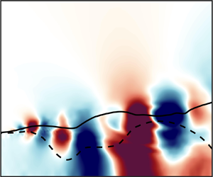
Hostname: page-component-745bb68f8f-cphqk Total loading time: 0 Render date: 2025-01-26T23:39:25.456Z Has data issue: false hasContentIssue false

Spectral proper orthogonal decomposition of harmonically forced turbulent flows

Published online by Cambridge University Press:  29 April 2024

Liam Heidt*
Affiliation:
Graduate Aerospace Laboratories of the California Institute of Technology, California Institute of Technology, Pasadena, CA 91101, USA
Tim Colonius
Affiliation:
Department of Mechanical and Civil Engineering, California Institute of Technology, Pasadena, CA 91101, USA
*
Email address for correspondence: lheidt@caltech.edu

Abstract

Many turbulent flows exhibit time-periodic statistics. These include turbomachinery flows, flows with external harmonic forcing and the wakes of bluff bodies. Many existing techniques for identifying turbulent coherent structures, however, assume the statistics are statistically stationary. In this paper, we leverage cyclostationary analysis, an extension of the statistically stationary framework to processes with periodically varying statistics, to generalize the spectral proper orthogonal decomposition (SPOD) to the cyclostationary case. The resulting properties of the cyclostationary SPOD (CS-SPOD for short) are explored, a theoretical connection between CS-SPOD and the harmonic resolvent analysis is provided, simplifications for the low and high forcing frequency limits are discussed, and an efficient algorithm to compute CS-SPOD with SPOD-like cost is presented. We illustrate the utility of CS-SPOD using two example problems: a modified complex linearized Ginzburg–Landau model and a high-Reynolds-number turbulent jet.

Type
JFM Papers
Copyright
© The Author(s), 2024. Published by Cambridge University Press

1. Introduction

Periodic and quasi-periodic forced turbulent flows are ubiquitous in engineering and nature. Such flows include those in turbomachinery, weather and climate, flow control with harmonic actuation, or any other flow that exhibits periodic/quasi-periodic modulation of the turbulence/statistics. In cases where the forcing is slow compared to the turbulence time scales, the statistics may be modelled as quasi-stationary (comprising a series of stationary states). However, in many cases, the forcing is at frequencies commensurate with the turbulence, and the turbulence structure is not only modulated by, but also altered by, the forcing. In such, a key goal is to identify coherent structures that can be compared with and contrasted to their occurrence in similar but unforced flows.

The most commonly used technique to identify coherent structures in turbulence is proper orthogonal decomposition (Lumley Reference Lumley1967, Reference Lumley1970; Aubry et al. Reference Aubry, Holmes, Lumley and Stone1988; Sirovich Reference Sirovich1989; Aubry Reference Aubry1991), which represents flow data as mutually orthogonal modes whose amplitudes optimally reconstruct the correlation tensor. When applied in its typical space-only form, the modes are not coherent in time, leading many researchers to apply dynamic mode decomposition and its variants (Rowley et al. Reference Rowley, Mezić, Bagheri, Schlatter and Henningson2009; Schmid Reference Schmid2010; Schmid et al. Reference Schmid, Li, Juniper and Pust2011). However, for statistically stationary flows, spectral proper orthogonal decomposition (SPOD) (Lumley Reference Lumley1967, Reference Lumley1970; Citriniti & George Reference Citriniti and George2000; Picard & Delville Reference Picard and Delville2000; Towne, Schmidt & Colonius Reference Towne, Schmidt and Colonius2018) leads to an optimal reconstruction of the space–time statistics and results in modes that oscillate at a single frequency. A fundamental assumption required in both space-only proper orthogonal decomposition (POD) and SPOD is statistical stationarity, meaning that the statistics are time invariant. This assumption is appropriate for many unforced flows. However, when forced, this fundamental assumption is no longer valid as the flow and its statistics are now correlated to the forcing. To clarify, by forcing, we mean any system that exhibits a periodic modulation of the statistics (including by actuators, vortex-shedding in bluff body flows, rotation in turbomachinery, etc.). Several works have developed extensions to SPOD to study forced turbulent flows. Franceschini et al. (Reference Franceschini, Sipp, Marquet, Moulin and Dandois2022) studied flows where a high-frequency turbulent component develops on a low-frequency periodic motion. Subsequently, a quasi-steady assumption is made and conditionally fixed coherent structures at each phase are determined. Glezer, Kadioglu & Pearlstein (Reference Glezer, Kadioglu and Pearlstein1989) developed an extended POD method for flows with periodic statistics by summing an ensemble of time series. However, since this method is based on POD, it still contains the shortcomings present in POD. Heidt et al. (Reference Heidt, Colonius, Nekkanti, Schmdit, Maia and Jordan2021) applied SPOD to the residual component of the triply decomposed fields (Hussain & Reynolds Reference Hussain and Reynolds1970, Reference Hussain and Reynolds1972) to isolate the impact of the forcing on the turbulence but still required a stationary assumption. Clearly, SPOD and the aforementioned extensions are not sufficient to study forced turbulent flows. This motivates an extension of SPOD to these flows, which is the primary focus of this paper which we achieve by leveraging cyclostationary analysis.

Cyclostationary analysis is an extension to statistically stationary analysis to processes with periodic statistics that have been applied in a range of fields (Gardner Reference Gardner2018), from economics to physics and mechanics. Initially developed by Gudzenko (Reference Gudzenko1959), Lebedev (Reference Lebedev1959) and Gladyshev (Reference Gladyshev1963), it was then extensively studied and popularized by Hurd (Reference Hurd1969) and Gardner (Reference Gardner1972). The theory of second-order cyclostationary processes was further developed by Boyles & Gardner (Reference Boyles and Gardner1983) and Gardner (Reference Gardner1986b), while Brown (Reference Brown1987) and Gardner (Reference Gardner1986c) furthered the theory of complex-valued processes. Cyclostationary analysis provides a robust statistical theory to study these processes, and tools analogous to those used to study stationary processes (e.g. the mean, cross-correlation, cross-spectral density, etc.) have been developed which naturally collapse back to their stationary counterparts when analysing a stationary process.

Kim, North & Huang (Reference Kim, North and Huang1996) developed cyclostationary empirical orthogonal-functions (CSEOFs) that essentially extends SPOD to cyclostationary processes for one-dimensional data. Kim & North (Reference Kim and North1997) modified this technique to include multi-dimensional data by reducing the computational cost through several approximations. However, due to a lack of clarity in the literature regarding the derivation, properties, interpretation and computation of these techniques, their use has been limited. Furthermore, despite the aforementioned approximations, both formulations are computationally intractable for high-dimensional data. In this paper, we extend SPOD to flows with time-periodic statistics through an extension to the exact form of CSEOFs (Kim et al. Reference Kim, North and Huang1996) to include large multi-dimensional data. We hereafter refer to this method as cyclostationary SPOD (CS-SPOD for short).

Methods used to model coherent structures are also considered. Specifically, we consider resolvent analysis (also known as input/output analysis), where one seeks forcing modes that give rise to the most amplified response modes with respect to their energetic gain. When applied to turbulent fluid flows, the nonlinear modal interactions are regarded as forcing terms to the linearized time-averaged turbulent mean (McKeon & Sharma Reference McKeon and Sharma2010). Resolvent analysis has been used to study a wide range of transitional and turbulent flows (Cossu, Pujals & Depardon Reference Cossu, Pujals and Depardon2009; McKeon & Sharma Reference McKeon and Sharma2010; Meliga, Pujals & Serre Reference Meliga, Pujals and Serre2012; Sharma & McKeon Reference Sharma and McKeon2013; Oberleithner, Paschereit & Wygnanski Reference Oberleithner, Paschereit and Wygnanski2014; Jeun, Nichols & Jovanović Reference Jeun, Nichols and Jovanović2016; Schmidt et al. Reference Schmidt, Towne, Rigas, Colonius and Brès2018), amongst others. Towne et al. (Reference Towne, Schmidt and Colonius2018) provided a theoretical connection between SPOD and resolvent, showing that resolvent output modes equal SPOD modes when the resolvent forcing modes are mutually uncorrelated. This provides a theoretical basis to use resolvent analysis to develop models of the space–time statistics of a turbulent flow (Moarref et al. Reference Moarref, Sharma, Tropp and McKeon2013; Towne, Lozano-Durán & Yang Reference Towne, Lozano-Durán and Yang2020; Amaral et al. Reference Amaral, Cavalieri, Martini, Jordan and Towne2021) and the development of various methods (Morra et al. Reference Morra, Semeraro, Henningson and Cossu2019; Pickering et al. Reference Pickering, Rigas, Schmidt, Sipp and Colonius2021a) to help whiten the forcing coefficients, thereby improving these models. Resolvent analysis was extended to flows with a time-periodic mean flow by Padovan, Otto & Rowley (Reference Padovan, Otto and Rowley2020) and Padovan & Rowley (Reference Padovan and Rowley2022), and is termed harmonic resolvent analysis. This leads to a system of frequency-coupled equations that provide the ability to study the first-order triadic interactions present in these time-periodic flows. Analogous to the relationship between SPOD and resolvent analysis, in the present paper, we establish a theoretical connection between CS-SPOD and harmonic resolvent analysis.

The remainder of the paper is organized as follows. Section 2 introduces the theory of cyclostationary processes and reviews an algorithm to compute their statistics. In § 3, CS-SPOD is derived, its properties explored and an efficient computational algorithm is proposed. After validating the method in § 4, we demonstrate the utility of CS-SPOD in § 5. In § 6, we explore the relationship between CS-SPOD and the harmonic resolvent analysis. Finally, in § 7, we investigate low- and high-frequency forcing limits. Section 8 concludes the manuscript and summarizes the main points.

2. Cyclostationary theory

This section provides an overview of the theory of cyclostationary analysis and the tools used to study them, with a focus on fluid dynamics. Comprehensive reviews can be found from Gardner, Napolitano & Paura (Reference Gardner, Napolitano and Paura2006), Antoni (Reference Antoni2009) and Napolitano (Reference Napolitano2019).

A complex-valued scalar process $q(t)$ at time $t$ is cyclostationary in the wide sense if its mean and autocorrelation functions are periodic with period $T_0$ (Gardner Reference Gardner1986b), giving

(2.1a)$$\begin{gather} E\{q(t)\} = E\{q(t + T_0)\}, \end{gather}$$
(2.1b)$$\begin{gather}R(t, \tau) = R(t + T_0, \tau), \end{gather}$$

where $E\{{\cdot }\}$ is the expectation operator, $R$ is the autocorrelation function and $\tau$ is a time delay. Since the mean and autocorrelation are time periodic, they can be expressed as a Fourier series

(2.2a)$$\begin{gather} E\{q(t)\} = \sum_{k_\alpha={-}\infty}^\infty \hat{q}_{k_\alpha \alpha_0} \,{\rm e}^{{\rm i}2{\rm \pi} (k_\alpha \alpha_0) t}, \end{gather}$$
(2.2b)$$\begin{gather}R(t, \tau) \equiv E\{q(t + \tau/2) q^*(t - \tau/2)\} = \sum_{k_\alpha={-}\infty}^\infty \hat{R}_{k_\alpha \alpha_0}(\tau) \,{\rm e}^{{\rm i}2{\rm \pi} (k_\alpha \alpha_0)t} , \end{gather}$$

where $k_\alpha \in \mathbb {Z}$ and the Fourier series coefficients are given by

(2.3a)$$\begin{gather} \hat{q}_{k_\alpha \alpha_0} \equiv \frac{1}{T_0} \int_{{-}T_0/2}^{T_0/2} E\{q(t)\} \,{\rm e}^{-{\rm i}2{\rm \pi} (k_\alpha \alpha_0) t} \,{\rm d}t, \end{gather}$$
(2.3b)$$\begin{gather}\hat{R}_{k_\alpha \alpha_0}(\tau) \equiv \frac{1}{T_0} \int_{{-}T_0/2}^{T_0/2} R(t, \tau) \,{\rm e}^{-{\rm i}2{\rm \pi} (k_\alpha \alpha_0) t} \,{\rm d}t, \end{gather}$$

where $\alpha _0 = 1/T_0$ is the fundamental cycle frequency and $({\cdot })^*$ is the complex conjugate. The Fourier coefficients $\hat {R}_{k_\alpha \alpha _0}(\tau )$ are known as the cyclic autocorrelation functions of $q(t)$ at cycle frequency $k_\alpha \alpha _0$. If a process contains non-zero $\hat {q}_{k_\alpha \alpha _0}$ and/or $\hat {R}_{k_\alpha \alpha _0}(\tau )$, it is said to exhibit first- and second-order cyclostationarity at cycle frequency $k_\alpha \alpha _0$, respectively. Wide-sense stationary processes are the special case where $\hat {R}_{k_\alpha \alpha _0}(\tau ) \ne 0$ for $k_\alpha = 0$ only.

If the process $q(t)$ contains a deterministic periodic component at cycle frequency $k_\alpha \alpha _0$, it would exhibit both first-order and second-order (and any higher order) cyclostationarity at cycle frequency $k_\alpha \alpha _0$. Thus, a deterministic component results in a pure first-order component and an impure (i.e. made up from components of a lower-order) second-order (or higher) component (Antoni et al. Reference Antoni, Bonnardot, Raad and El Badaoui2004). Antoni et al. (Reference Antoni, Bonnardot, Raad and El Badaoui2004) and Antoni (Reference Antoni2009) showed that in physical systems, it is crucial to analyse the first- and second-order components separately, where the second-order component $q^{\prime \prime }(t)$ is defined as

(2.4)\begin{equation} q^{\prime\prime}(t) \equiv q(t) - E\{q(t)\}, \end{equation}

such that $q(t) = E\{q(t)\} + q^{\prime \prime }(t)$ and the mean $E\{q(t)\} = E\{q(t + T_0)\}$ is $T_0$ periodic. This approach makes physical sense considering that the first-order component is the deterministic tonal component that originates from the forcing, while the second-order component is a stochastic component that represents the underlying turbulence that is modified by the forcing. The sequential approach is analogous to the triple decomposition (Hussain & Reynolds Reference Hussain and Reynolds1970, Reference Hussain and Reynolds1972) where the underlying flow is separated into the first-order (phase-averaged) and second-order (turbulent/residual) components. First-order and second-order cyclostationarity then refer to a modulation of the first-order and second-order components, respectively.

In this manuscript, we assume that all processes analysed using second-order analysis tools are zero-mean processes (or have had their first-order component removed). Thus, by stating that a process exhibits second-order cyclostationarity at cycle frequency $k_\alpha \alpha _0$, we mean that the process exhibits pure second-order cyclostationarity at $k_\alpha \alpha _0$.

We must clarify one point of terminology. Considering stationary processes are a subset of cyclostationary processes, all stationary processes are also cyclostationary. We use the most restrictive description, i.e. stationary processes are referred to as stationary and not cyclostationary. By stating that a process exhibits cyclostationarity, we imply that at least one cycle frequency $k_\alpha \alpha _0$, $k_\alpha \ne 0$ exists.

2.1. Second-order cyclostationary analysis tools

In fluid dynamics, we are frequently interested in the correlation between two quantities. Thus, we will now consider the complex-valued vector-valued process $\boldsymbol {q}(\boldsymbol {x}, t)$ at time $t$ and independent variables (or spatial locations) $\boldsymbol {x}$ instead of the scalar process $q(t)$. Two processes are jointly cyclostationary if their cross-correlation function can be expressed as a Fourier series, such that

(2.5)\begin{align} \boldsymbol{R}(\boldsymbol{x}, \boldsymbol{x}^\prime, t, \tau) &\equiv E\{\boldsymbol{q}(\boldsymbol{x}, t+\tau/2)\boldsymbol{q}^*(\boldsymbol{x}^\prime, t - \tau/2)\}\nonumber\\ & =\sum_{k_\alpha={-}\infty}^\infty \hat{\boldsymbol{R}}_{k_\alpha \alpha_0}(\boldsymbol{x}, \boldsymbol{x}^\prime, \tau) \,{\rm e}^{{\rm i}2{\rm \pi}(k_\alpha \alpha_0) t}, \end{align}

where the Fourier series coefficients are given by

(2.6)\begin{equation} \hat{\boldsymbol{R}}_{k_\alpha \alpha_0}(\boldsymbol{x}, \boldsymbol{x}^\prime, \tau) \equiv \frac{1}{T_0} \int_{{-}T_0/2}^{T_0/2} \boldsymbol{R}(\boldsymbol{x}, \boldsymbol{x}^\prime, t, \tau) \,{\rm e}^{-{\rm i}2{\rm \pi} (k_\alpha \alpha_0) t} \,{\rm d}t, \end{equation}

and are known as the cyclic cross-correlation functions between $\boldsymbol {q}(\boldsymbol {x})$ and $\boldsymbol {q}(\boldsymbol {x}^\prime )$ at cycle frequency $k_\alpha \alpha _0$. If the only non-zero cycle frequency is $k_\alpha \alpha _0 = 0$, then $\boldsymbol {q}(\boldsymbol {x})$ and $\boldsymbol {q}(\boldsymbol {x}^\prime )$ are jointly wide-sense stationary. Similar to the common assumption in stationary analysis, we assume that all processes are separately and jointly cyclostationary.

A cyclostationary process can be analysed in the dual-frequency domain via the cyclic cross-spectral density (CCSD). The CCSD is the generalization of the cross-spectral density (CSD) for cyclostationary processes and is related to the cyclic cross-correlation function via the cyclic Wiener–Khinchin relation (Gardner & Robinson Reference Gardner and Robinson1989)

(2.7)\begin{equation} {\boldsymbol{S}}_{k_\alpha \alpha_0}(\boldsymbol{x}, \boldsymbol{x}^\prime, f) = \int_{-\infty}^\infty \hat{\boldsymbol{R}}_{k_\alpha \alpha_0}(\boldsymbol{x}, \boldsymbol{x}^\prime, \tau) \,{\rm e}^{-{\rm i}2{\rm \pi} f\tau} \,{\rm d}\tau. \end{equation}

The CCSD can also be written as

(2.8) \begin{align} & {\boldsymbol{S}}_{k_\alpha \alpha_0}(\boldsymbol{x}, \boldsymbol{x}^\prime, f) \nonumber\\ &\quad \equiv \lim_{\Delta f \rightarrow 0} \lim_{T \rightarrow \infty} \frac{1}{T} \int_{{-}T/2}^{T/2} \Delta f \,E\left\{\hat{\boldsymbol{q}}_{1/\Delta f} \left(\boldsymbol{x}, t, f + \frac{1}{2} k_\alpha \alpha_0\right) \hat{\boldsymbol{q}}^*_{1/\Delta f} \left(\boldsymbol{x}^\prime, t, f - \frac{1}{2} k_\alpha \alpha_0\right) \right\}\,{\rm d}t, \end{align}

where $\hat {\boldsymbol {q}}_{W} (\boldsymbol {x}, t, f) \equiv \int _{t - {W}/{2}}^{t + {W}/{2}} \boldsymbol {q}(\boldsymbol {x}, t^\prime ) \,{\rm e}^{-{\rm i}2{\rm \pi} f t^\prime } \,{\rm d}t^\prime$ is the short-time Fourier transform of $\boldsymbol {q}(\boldsymbol {x}, t)$, $f$ is the spectral frequency and $k_\alpha \alpha _0$ is the cycle frequency. This shows that the CCSD represents the time-averaged statistical correlation (with zero lag) of two spectral components at frequencies $f + \frac {1}{2} k_\alpha \alpha _0$ and $f - \frac {1}{2} k_\alpha \alpha _0$ as the bandwidth approaches zero (Napolitano Reference Napolitano2019). Formally, the CCSD is defined as in (2.8) and then the Fourier transform version (2.7) is proved, which is then known as the Gardner relation or as the cyclic Wiener–Khinchin relation (Napolitano Reference Napolitano2019). For $k_\alpha = 0$, the CCSD naturally reduces to the CSD, i.e. $\boldsymbol {S}_0(\boldsymbol {x}, \boldsymbol {x}^\prime, f)$. Correlation between spectral components in cyclostationary processes is critical in the derivation of CS-SPOD, and for stationary processes, the lack of correlation between spectral components is why SPOD can analyse each frequency independently.

The Wigner–Ville (WV) spectrum (Martin Reference Martin1982; Martin & Flandrin Reference Martin and Flandrin1985; Antoni Reference Antoni2007) shows the spectral information of the process as a function of time (or phase) and, for a cyclostationary process, is given by

(2.9)\begin{equation} \boldsymbol{WV}(\boldsymbol{x}, \boldsymbol{x}^\prime, t, f) = \sum_{k_\alpha={-}\infty}^\infty \boldsymbol{S}_{k_\alpha \alpha_0}(\boldsymbol{x}, \boldsymbol{x}^\prime, f)\,{\rm e}^{{\rm i}2{\rm \pi} (k_\alpha \alpha_0) t}. \end{equation}

The WV spectrum of the cyclic power-spectral density is determined by setting $\boldsymbol {x} = \boldsymbol {x}^\prime$, giving $\boldsymbol {WV}(\boldsymbol {x}, t, f) = \sum _{k_\alpha =-\infty }^\infty \boldsymbol {S}_{k_\alpha \alpha _0}(\boldsymbol {x}, f)\,{\rm e}^{{\rm i}2{\rm \pi} (k_\alpha \alpha _0) t}$. While non-physical, the WV spectrum may contain negative energy densities due to the negative interaction terms in the WV spectrum (Flandrin Reference Flandrin1998; Antoni Reference Antoni2007). However, Antoni (Reference Antoni2007) showed this could be arbitrarily reduced with increasing sampling time. The CCSD and WV spectrum can be integrated with respect to frequency (Gardner Reference Gardner1994; Randall, Antoni & Chobsaard Reference Randall, Antoni and Chobsaard2001), which results in the instantaneous variance and the cyclic distribution of the instantaneous variance, respectively

(2.10a)$$\begin{gather} \boldsymbol{m}(\boldsymbol{x}, t) = E\{\boldsymbol{q}(\boldsymbol{x}, t)\boldsymbol{q}^*(\boldsymbol{x}, t)\} = \int_{-\infty}^\infty \boldsymbol{WV}(\boldsymbol{x}, t, f) \,{\rm d}f, \end{gather}$$
(2.10b)$$\begin{gather}\hat{\boldsymbol{m}}_{k_\alpha \alpha_0}(\boldsymbol{x}) = \int_{-\infty}^\infty \boldsymbol{S}_{k_\alpha \alpha_0}(\boldsymbol{x}, f) \,{\rm d}f, \end{gather}$$

where ${\boldsymbol {m}}(\boldsymbol {x}, t)$ is the mean-variance of the process and $\hat {\boldsymbol {m}}_{k_\alpha \alpha _0}(\boldsymbol {x})$ quantifies the mean-variance contribution from each cycle frequency $k_\alpha \alpha _0$.

So far, we have assumed that the cycle frequencies are known, but this may not always be the case. To determine the cycle frequencies present in the system, all possible cycle frequencies $\alpha$ are explored by rewriting the CCSD as

(2.11)\begin{align} & {\boldsymbol{S}}(\boldsymbol{x}, \boldsymbol{x}^\prime, \alpha, f) \nonumber\\ &\quad \equiv \lim_{\Delta f \rightarrow 0} \lim_{T \rightarrow \infty} \frac{1}{T} \int_{{-}T/2}^{T/2} \Delta f\, E\left\{\hat{\boldsymbol{q}}_{1/\Delta f} \left(\boldsymbol{x}, t, f + \frac{\alpha}{2}\right) \hat{\boldsymbol{q}}^*_{1/\Delta f} \left(\boldsymbol{x}^\prime, t, f - \frac{\alpha}{2}\right) \right\}\,{\rm d}t. \end{align}

A process exhibits cyclostationarity at cycle frequency $\alpha$ when ${\boldsymbol {S}}(\boldsymbol {x}, \boldsymbol {x}^\prime, \alpha, f) \ne 0$. For cyclostationary processes, because the cross-correlation function is periodic, the spectral correlation becomes discrete in $\alpha$ such that

(2.12)\begin{equation} \boldsymbol{S}(\boldsymbol{x}, \boldsymbol{x}^\prime, \alpha, f) = \sum_{k_\alpha={-}\infty}^\infty \boldsymbol{S}_{k_\alpha \alpha_0}(\boldsymbol{x}, \boldsymbol{x}^\prime, f) \delta (\alpha - k_\alpha \alpha_0), \end{equation}

where $\delta$ is the Kronecker delta. The cyclic distribution of the instantaneous variance is rewritten as

(2.13)\begin{equation} \hat{\boldsymbol{m}}(\boldsymbol{x}, \alpha) = \int_{-\infty}^\infty \boldsymbol{S}(\boldsymbol{x}, \alpha, f) \,{\rm d}f, \end{equation}

which similarly becomes discrete for a cyclostationary process.

2.2. Cycloergodicity

In fluid dynamics, it is laborious to require multiple realizations of a single process, and we often invoke ergodicity in stationary processes to equate the ensemble average with a long-time average of a single realization. We can similarly leverage the concept of cycloergodicity as described by Boyles & Gardner (Reference Boyles and Gardner1983), allowing us to replace the expectation operator with a suitable time average, specifically, the cycle-averaging operator (Braun Reference Braun1975)

(2.14)\begin{equation} \tilde{\boldsymbol{q}}(\boldsymbol{x}, t) = E\{\boldsymbol{q}(\boldsymbol{x}, t)\} = \lim_{P \rightarrow \infty} \frac{1}{P} \sum_{p = 0}^P \boldsymbol{q}(\boldsymbol{x}, t + pT_0), \end{equation}

where $\tilde {\boldsymbol {q}}(\boldsymbol {x}, t)$ is the mean. The cycle-averaging operator is used when the data are phase-locked to the forcing (i.e. sampled at an integer number of samples per cycle) and is identical to the phase-average used in the triple decomposition (Hussain & Reynolds Reference Hussain and Reynolds1970; Reynolds & Hussain Reference Reynolds and Hussain1972). As the cycle-averaging operator is periodic, it can be expressed as a Poisson sum

(2.15)\begin{equation} \tilde{\boldsymbol{q}}(\boldsymbol{x}, t) = E\{\boldsymbol{q}(\boldsymbol{x}, t)\} = \sum_{k_\alpha={-}\infty}^\infty {\rm e}^{{\rm i}2{\rm \pi} (k_\alpha \alpha_0) t} \lim_{s\rightarrow \infty} \frac{1}{s}\int_{{-}s/2}^{s/2} \boldsymbol{q}(\boldsymbol{x}, t^\prime)\,{\rm e}^{-{\rm i}2{\rm \pi} (k_\alpha \alpha_0) t^\prime} \,{\rm d}t^\prime. \end{equation}

This definition is employed for non-phase-locked data or to filter out first-order components that are assumed to be statistical noise (Sonnenberger, Graichen & Erk Reference Sonnenberger, Graichen and Erk2000; Franceschini et al. Reference Franceschini, Sipp, Marquet, Moulin and Dandois2022) and is identical to the harmonic-averaging procedure used by Mezić (Reference Mezić2013) and Arbabi & Mezić (Reference Arbabi and Mezić2017) when restricted to a temporally periodic average.

2.3. Computing the CCSD

There are practical considerations and nuances to computing the CCSD from discrete data that we discuss in this section. Let the vector q$_k \in \mathbb {C}^N$ represent a flow snapshot, i.e. the instantaneous state of the process $\boldsymbol {q}(\boldsymbol {x}, t)$ at time $t_k$ on a set of points in a spatial domain $\varOmega$. The length of the vector $N$ is equal to the number of spatial points multiplied by the number of state variables. We assume that these data are available for $M$ equispaced snapshots, with $t_{k+1} = t_k + \Delta t$. In addition, we assume that these data are phase-locked, meaning that there are an integer number of time steps in the fundamental period, $T_0$, and define $N_\theta =T_0/\Delta t$. This restriction simplifies and reduces the computational expense of the calculations but can in principle be relaxed by using the Poisson sum time-average as in (2.15) and the non-computationally efficient form of CS-SPOD shown in . Alternatively, non-phased-locked data can be temporally interpolated to be phase-locked. Adopting similar notation to Towne et al. (Reference Towne, Schmidt and Colonius2018), we estimate the CCSD tensor $\boldsymbol {S}(\boldsymbol {x}, \boldsymbol {x}^\prime, \alpha, f)$, which represents the spectral correlation between $\boldsymbol {q}(\boldsymbol {x}, t)$ and $\boldsymbol {q}(\boldsymbol {x}^\prime, t)$ at cycle frequency $\alpha$ and spectral frequency $f$. For a cyclostationary process, $\boldsymbol {S}(\boldsymbol {x}, \boldsymbol {x}^\prime, \alpha, f)$ is non-zero for $\alpha = k_\alpha \alpha _0$ only, and therefore is written as $\boldsymbol {S}_{k_\alpha \alpha _0}(\boldsymbol {x}, \boldsymbol {x}^\prime, f)$ or equivalently $\boldsymbol {S}_{k_\alpha /T_0}(\boldsymbol {x}, \boldsymbol {x}^\prime, f)$. The space–time data can now be represented as the data matrix Q and time vector T:

(2.16) $$\begin{gather} \textbf{Q} = [\textbf{q}_1, \textbf{q}_2, \ldots, \textbf{q}_M] \in \mathbb{C}^{N\times M}, \end{gather}$$
(2.17)$$\begin{gather}\textbf{T} = [t_1, t_2, \ldots, t_M] \in \mathbb{R}^{M}. \end{gather}$$

Although we have a formula for the CCSD as seen in (2.8) and (2.11), this does not result in a consistent estimator of the CCSD, as the variance of the estimate of the CCSD does not tend to zero as the amount of available data becomes large (Jenkins Reference Jenkins1968; Antoni Reference Antoni2007; Napolitano Reference Napolitano2019). Instead, this results in an estimate where the variance in the estimate is equal to the squared value of the estimate itself. A consistent estimate of the CCSD can be obtained by employing an appropriate averaging technique. The most common technique is the time-averaging Welch method (Welch Reference Welch1967) due to its high computational efficiency. The Welch method averages a number of CCSDs to obtain a consistent estimate of the CCSD. From (2.11), we see that to compute the CCSD, the Welch procedure is performed on two frequency-shifted versions of the data, given by

(2.18a) \begin{align} \textbf{Q}_{{\pm} \alpha/2} &= \textbf{Q} \,{\rm e}^{-{\rm i} 2{\rm \pi} ({\pm} \alpha/2) \textbf{T}} = [{\textbf{q}}_{1, \pm \alpha/2},{\textbf{q}}_{2, \pm \alpha/2}, \ldots, {\textbf{q}}_{M, \pm \alpha/2} ], \end{align}
(2.18b) \begin{align} &= [{\textbf{q}}_{1} \,{\rm e}^{-{\rm i} 2{\rm \pi} ({\pm} \alpha/2) t_1}, {\textbf{q}}_{2} \,{\rm e}^{-{\rm i} 2{\rm \pi} ({\pm} \alpha/2) t_2}, \ldots, {\textbf{q}}_{M} \,{\rm e}^{-{\rm i} 2{\rm \pi} ({\pm} \alpha/2) t_M}], \end{align}

where ${\textbf{q}}_{k, \pm \alpha /2}$ are the $\pm \frac {1}{2}\alpha$ frequency-shifted data matrices corresponding to the $k$th snapshot, i.e. ${\textbf{q}}_{k, \pm \alpha /2} = {\textbf{q}}_{k} \,{\rm e}^{-{\rm i} 2{\rm \pi} (\pm \alpha /2) t_k}$. Next, we split the two frequency-shifted data matrices into a number of, possibly overlapping, blocks. Each block is written as

(2.19) \begin{equation} \textbf{Q}^{(n)}_{{\pm} \alpha/2} = [\textbf{q}_{1,\pm \alpha/2}^{(n)},\textbf{q}_{2,\pm \alpha/2}^{(n)}, \ldots, \textbf{q}_{N_f,\pm \alpha/2}^{(n)} ] \in \mathbb{C}^{N\times N_f}, \end{equation}

where $N_f$ is the number of snapshots in each block and the $k$th entry of the $n$th block is $\textbf{q}^{(n)}_{k,\pm \alpha /2} = \textbf{q}_{k+(n-1)(N_f - N_0), \pm \alpha /2}$. The total number of blocks, $N_b$, is given by $N_b = \lfloor {(M - N_0)}/{(N_f - N_0)}\rfloor$, where $\lfloor {\cdot } \rfloor$ represents the floor operator and $N_0$ is the number of snapshots that each block overlaps. The cycloergodicity hypothesis states that each of these blocks is considered to be a single realization in an ensemble of realizations of this cyclostationary flow. Subsequently, the discrete Fourier transform (DFT) of each block for both frequency-shifted matrices is computed using a window $w$, giving

(2.20) \begin{equation} \hat{\textbf{Q}}^{(n)}_{{\pm} \alpha/2} = [\hat{\textbf{q}}_{ 1, \pm \alpha/2}^{(n)},\hat{\textbf{q}}_{2, \pm \alpha/2}^{(n)}, \ldots, \hat{\textbf{q}}_{N_f, \pm \alpha/2}^{(n)} ], \end{equation}

where

(2.21) \begin{equation} \hat{\textbf{q}}_{k, \pm \alpha/2}^{(n)} = \frac{1}{\sqrt{N_f}} \sum_{j = 1}^{N_f} {w_j}{\textbf{q}}_{j, \pm \alpha/2}^{(n)} \,{\rm e}^{-{\rm i}2{\rm \pi} (k-1)[(j - 1)/N_f]} \end{equation}

for $k = 1, \ldots, N_f$ and $n = 1, \ldots, N_b$, where $\hat {\textbf{q}}^{(n)}_{k, \pm \alpha /2}$ is the $k$th Fourier component of the $n$th block of the $\pm \alpha /2$ frequency-shifted data matrix, i.e. $f_{k, \pm \alpha _0/2}$. The nodal values $w_j$ of a window function are used to mitigate spectral and cyclic leakage arising from the non-periodicity of the data within each block. Due to the $\pm \alpha /2$ frequency-shifting applied, the $k$th discrete frequencies of the $\pm \alpha /2$ frequency-shifted data matrices represent a frequency of

(2.22) \begin{equation} f_{k, \pm \alpha/2} = f_{k} \pm \frac{\alpha}{2} = \begin{cases} \dfrac{k-1}{N_f\Delta t} & \text{for } k \leq N_f/2, \\ \dfrac{k-1 - N_f}{N_f \Delta t} & \text{for } k > N_f/2, \end{cases} \pm \frac{\alpha}{2}. \end{equation}

This shows that the frequency components $f_k + \alpha /2$ and $f_k - \alpha /2$, as required by (2.11), have the same index $k$ in the shifted frequency vectors $f_{k, \pm \alpha /2}$. The CCSD tensor $\boldsymbol {S}(\boldsymbol {x}, \boldsymbol {x}^\prime, \alpha, f)$ is then estimated at cycle frequency $\alpha$ and spectral frequency $f_k$ by

(2.23) \begin{equation} \textbf{S}_{f_k, \alpha} = \frac{\Delta t}{s N_b} \sum_{n =1}^{N_b} \hat{\textbf{q}}^{(n)}_{k, \alpha/2} (\hat{\textbf{q}}^{(n)}_{k, -\alpha/2})^*, \end{equation}

where $s = \sum _{j = 1}^{N_f}w_j^2$ is the normalization constant that accounts for the difference in power between the windowed and non-windowed signal. This is written compactly by arranging the Fourier coefficients at the same index $k$ into new frequency-data matrices

(2.24) \begin{equation} \hat{\textbf{Q}}_{f_k, \pm \alpha/2} = \sqrt{\kappa} [\hat{\textbf{q}}_{k, \pm \alpha/2}^{(1)}, \hat{\textbf{q}}_{k, \pm \alpha/2}^{(2)}, \ldots, \hat{\textbf{q}}_{k, \pm \alpha/2}^{(N_b-1)}, \hat{\textbf{q}}_{k, \pm \alpha/2}^{(N_b)}] \in \mathbb{C}^{N\times N_b}, \end{equation}

where $\kappa = {\Delta t}/{s N_b}$. Then, $\boldsymbol {S}_{f_k, \alpha }$ is estimated by

(2.25)\begin{equation} \textbf{S}_{f_k, \alpha} = \hat{\textbf{Q}}_{f_k, \alpha/2} (\hat{\textbf{Q}}_{f_k, -\alpha/2})^*. \end{equation}

This estimate converges, i.e. the bias and variance become zero, as $N_b$ and $N_f$ are increased together (Welch Reference Welch1967; Antoni Reference Antoni2007; Bendat & Piersol Reference Bendat and Piersol2011). The algorithm to compute the CCSD from data snapshots is outlined in , from which all other second-order cyclostationary analysis tools can be computed. For efficient memory management, variables assigned with ‘$\leftarrow$’ can be deleted after each iteration in their respective loop. Similar to the Welch estimate of the CSD, the estimate of the CCSD suffers from the standard bias-variance trade-off, and caution should be taken to ensure sufficiently converged statistics. In the CCSD, a phenomenon similar to spectral leakage is present and is called cyclic leakage (Gardner Reference Gardner1986a) that results in erroneous cycle frequencies. Using $67\,\%$ overlap when using a Hanning or Hamming window results in excellent cyclic leakage minimization and variance reduction (Antoni Reference Antoni2007). To reduce the variance sufficiently, $T\Delta f \gg 1$ is required (Antoni Reference Antoni2009). If one does not know the cycle frequencies a priori, one must search over all possible cycle frequencies with a resolution $\Delta \alpha = 1/T$ (Gardner Reference Gardner1986a) to ensure all cycle frequencies are captured.

Algorithm 1 Algorithm to compute the CCSD.

3. Cyclostationary SPOD

3.1. Derivation

The objective of CS-SPOD is to find deterministic functions that best approximate, on average, a zero-mean stochastic process. For clarity, we derive CS-SPOD using an approach and notation analogous to the SPOD derivation presented by Towne et al. (Reference Towne, Schmidt and Colonius2018) and refer the reader to Brereton & Kodal (Reference Brereton and Kodal1992), Towne et al. (Reference Towne, Schmidt and Colonius2018) and Schmidt & Colonius (Reference Schmidt and Colonius2020) for detailed discussions on POD and SPOD. Like SPOD, we seek deterministic modes that depend on both space and time such that we can optimally decompose the space–time statistics of the flow. Thus, we assume that each realization of the stochastic process belongs to a Hilbert space with an inner product

(3.1)\begin{equation} \langle \boldsymbol{q}_1, \boldsymbol{q}_2 \rangle_{x,t} = \int_{-\infty}^\infty \int_{\varOmega} \boldsymbol{q}_2^*(\boldsymbol{x}, t) \boldsymbol{W}(\boldsymbol{x}) \boldsymbol{q}_1(\boldsymbol{x}, t) \,\mathrm{d}\kern 0.06em \boldsymbol{x} \,\mathrm{d}t, \end{equation}

where $\boldsymbol {q}_1(\boldsymbol {x}, t),\ \boldsymbol {q}_2(\boldsymbol {x}, t)$ are two realizations of the flow, $\boldsymbol {W}(\boldsymbol {x})$ is a positive-definite weighting tensor (while we have chosen a time-independent weighting tensor since this simplifies the derivations and is appropriate for the example cases shown, a time-periodic weighting tensor could also be employed), and $\varOmega$ denotes the spatial domain of interest. We then seek to maximize

(3.2)\begin{equation} \lambda = \frac{E\{|\langle \boldsymbol{q}(\boldsymbol{x}, t), \boldsymbol{\phi}(\boldsymbol{x}, t)\rangle_{x,t}|^2\}}{\langle \boldsymbol{\phi}(\boldsymbol{x}, t), \boldsymbol{\phi}(\boldsymbol{x}, t)\rangle_{x,t}}, \end{equation}

which leads to

(3.3)\begin{equation} \int_{-\infty}^\infty \int_{\varOmega} \boldsymbol{R}(\boldsymbol{x}, \boldsymbol{x}^\prime, t, t^\prime) \boldsymbol{W}(\boldsymbol{x}^\prime) \boldsymbol{\phi}(\boldsymbol{x}^\prime, t^\prime) \,\mathrm{d}\kern 0.06em \boldsymbol{x}^\prime \,\mathrm{d}t^\prime = \lambda \boldsymbol{\phi}(\boldsymbol{x}, t), \end{equation}

where $\boldsymbol {R}(\boldsymbol {x}, \boldsymbol {x}^\prime, t, t^\prime ) \equiv E\{\boldsymbol {q}(\boldsymbol {x}, t)\boldsymbol {q}^*(\boldsymbol {x}^\prime, t^\prime )\}$ is the two-point space–time correlation tensor. Until this stage, no assumptions about the flow have been made and it is therefore identical to the derivation of SPOD (Lumley Reference Lumley1967, Reference Lumley1970; Towne et al. Reference Towne, Schmidt and Colonius2018).

Since cyclostationary flows persist indefinitely, they have infinite energy in the space–time norm, as shown in (3.1). Consequently, the eigenmodes of (3.3) do not possess any of the useful quantities relied upon in POD or SPOD. To solve this, a new eigenvalue decomposition is obtained in the spectral domain from which modes with the desired properties are determined. We employ a solution ansatz of

(3.4)\begin{equation} \boldsymbol{\phi}(\boldsymbol{x}, t) = \sum_{k_f ={-}\infty}^\infty \boldsymbol{\psi}(\boldsymbol{x}, \gamma + k_f\alpha_0) \,{\rm e}^{{\rm i}2{\rm \pi} (\gamma + k_f\alpha_0)t}. \end{equation}

The set of frequencies present in the solution ansatz $\boldsymbol {\phi }(\boldsymbol {x}, t)$ is called the $\gamma$ set of solution frequencies $\mathcal {\varOmega }_{\gamma } = \{\ldots,\ \gamma - 2\alpha _0,\ \gamma - \alpha _0, \gamma,\ \gamma + \alpha _0,\ \gamma + 2\alpha _0,\ \ldots \}$.

In Appendix A, we then use theory from § 2 to derive the infinite-dimensional CS-SPOD eigenvalue problem, written compactly as

(3.5)\begin{equation} \int_{\varOmega} {{\boldsymbol{\mathsf{S}}}}(\boldsymbol{x}, \boldsymbol{x}^\prime, \gamma) \boldsymbol{\mathsf{W}}(\boldsymbol{x}^\prime) \boldsymbol{\varPsi}(\boldsymbol{x}^\prime, \gamma)\, \mathrm{d}\kern 0.06em \boldsymbol{x}^\prime = \lambda(\gamma) \boldsymbol{\varPsi}(\boldsymbol{x}, \gamma), \end{equation}

where

(3.6a) \begin{align} &{{\boldsymbol{\mathsf{S}}}}(\boldsymbol{x}, \boldsymbol{x}^\prime, \gamma) \nonumber\\ &\ =\begin{bmatrix} \ddots & \ddots & \ddots & \ddots & \ddots \\ \ddots & \boldsymbol{S}_0(\boldsymbol{x}, \boldsymbol{x}^\prime, \gamma - \alpha_0) & \boldsymbol{S}_{-\alpha_0}\left(\boldsymbol{x}, \boldsymbol{x}^\prime, \gamma - \dfrac{\alpha_0}{2} \right) & \boldsymbol{S}_{{-}2\alpha_0}(\boldsymbol{x}, \boldsymbol{x}^\prime,\gamma) & \ddots\\ \ddots & \boldsymbol{S}_{\alpha_0}\left(\boldsymbol{x}, \boldsymbol{x}^\prime,\gamma- \dfrac{\alpha_0}{2}\right) & \boldsymbol{S}_0(\boldsymbol{x}, \boldsymbol{x}^\prime,\gamma) & \boldsymbol{S}_{-\alpha_0}\left(\boldsymbol{x}, \boldsymbol{x}^\prime,\gamma+ \dfrac{\alpha_0}{2} \right) & \ddots\\ \ddots & \boldsymbol{S}_{2\alpha_0}(\boldsymbol{x}, \boldsymbol{x}^\prime,\gamma) & \boldsymbol{S}_{\alpha_0}\left(\boldsymbol{x}, \boldsymbol{x}^\prime,\gamma+ \dfrac{\alpha_0}{2} \right) & \boldsymbol{S}_0(\boldsymbol{x}, \boldsymbol{x}^\prime,\gamma+ \alpha_0) & \ddots\\ \ddots & \ddots & \ddots & \ddots & \ddots \end{bmatrix},\nonumber\\ \end{align}
(3.6b,c)\begin{gather} {{\boldsymbol{\mathsf{W}}}}(\boldsymbol{x}) =\begin{bmatrix} \ddots & & & & \\ & \hspace{-2mm}\boldsymbol{W}(\boldsymbol{x}) & & & \\ & & \hspace{-2mm}\boldsymbol{W}(\boldsymbol{x}) & & \\ & & & \hspace{-2mm}\boldsymbol{W}(\boldsymbol{x}) & \\ & & & & \hspace{-2mm}\ddots \end{bmatrix},\quad \boldsymbol{\varPsi}(\boldsymbol{x}, \gamma) =\begin{bmatrix} \vdots\\ \boldsymbol{\psi}(\boldsymbol{x},\gamma- \alpha_{0})\\ \boldsymbol{\psi}(\boldsymbol{x},\gamma)\\ \boldsymbol{\psi}(\boldsymbol{x},\gamma+ \alpha_{0})\\ \vdots \end{bmatrix}. \end{gather}

Here, ${{\boldsymbol{\mathsf{S}}}}(\boldsymbol {x}, \boldsymbol {x}^\prime, \gamma )$ is the CS-SPOD decomposition tensor, ${{\boldsymbol{\mathsf{W}}}}(\boldsymbol {x})$ is the concatenated weight tensor and $\boldsymbol {\varPsi }(\boldsymbol {x}, \gamma )$ are the CS-SPOD eigenvectors. This frequency-domain version $\boldsymbol {\varPsi }(\boldsymbol {x}, \gamma )$ of the CS-SPOD eigenvectors can be converted to the time-domain version $\boldsymbol {\phi }(\boldsymbol {x}, t)$ using (3.4). In essence, we convert the original problem into the frequency domain and then solve for the Fourier series coefficients $\boldsymbol {\psi }(\boldsymbol {x}, f)$ at each $f \in \mathcal {\varOmega }_{\gamma }$.

This coupling of frequencies in CS-SPOD occurs because frequency components separated by $k_\alpha \alpha _0$ are correlated to each other, as shown in (2.8). In contrast, stationary processes do not exhibit correlation between frequencies, and thus each frequency can be solved independently via SPOD. Due to this coupling, CS-SPOD performed at $\gamma$ and $\gamma + \alpha _0$ solve the same problem, i.e. giving $\mathcal {\varOmega }_{\gamma } = \mathcal {\varOmega }_{\gamma +z \alpha _0}$, where $z \in \mathbb {Z}$. This means that CS-SPOD only contains unique solutions for the frequency sets corresponding to $\gamma \in \varGamma$, where $\varGamma = [-\alpha _0/2,\ \alpha _0/2)$.

In practice, the infinite-dimensional problem can not be solved. Instead, we must restrict the cycle frequencies considered and the frequencies present in the solution ansatz to some limit. We restrict the solution ansatz to

(3.7)\begin{equation} \boldsymbol{\phi}(\boldsymbol{x}, t) = \sum_{k_f ={-}K_f}^{K_f} \boldsymbol{\psi}(\boldsymbol{x}, \gamma + k_f\alpha_0) \,{\rm e}^{{\rm i}2{\rm \pi} (\gamma + k_f\alpha_0)t} \end{equation}

and the cycle frequencies to

(3.8)\begin{equation} \boldsymbol{R}(\boldsymbol{x}, \boldsymbol{x}^\prime, t, \tau) = \sum_{k_\alpha ={-}K_\alpha}^{K_\alpha} \widetilde{\boldsymbol{R}}_{k_\alpha \alpha_0}(\boldsymbol{x}, \boldsymbol{x}^\prime, \tau) \,{\rm e}^{{\rm i}2{\rm \pi} (k_\alpha \alpha_0) t}, \end{equation}

where $K_f \in \mathbb {Z}^+$ and $K_\alpha \in \mathbb {Z}^+$. This gives a final solution frequency set of $\mathcal {\varOmega }_{\gamma } = \{-K_f\alpha _0 + \gamma, (-K_f+1)\alpha _0 + \gamma,\ \ldots, \gamma,\ \ldots, (K_f-1)\alpha _0+ \gamma, K_f\alpha _0+ \gamma \}$. In addition, the flow may only exhibit cyclostationarity at $K_\alpha$ harmonics of the fundamental cycle frequency. We employ identical notation to restrict the harmonics used to compute various second-order tools, such as the WV spectrum. These limits result in $2 K_f+1$ coupled equations, resulting in a $2K_f+1 \times 2K_f+1$ block eigensystem that is $2 K_\alpha +1$ banded-block-diagonal. In practice, $K_f$ should be chosen such that $\mathcal {\varOmega }_{\gamma }$ encompasses all frequencies of interest/importance, $K_\alpha$ should be chosen to encompass all the cycle frequencies present in the flow and $K_\alpha \le K_f$. An example for $K_f = 2, K_\alpha = 1$ is (for compactness, we have dropped the explicit dependence on $\boldsymbol {x}$ in this equation)

(3.9) \begin{align} {{\boldsymbol{\mathsf{S}}}}(\gamma) =\begin{bmatrix} \boldsymbol{S}_{0}(\gamma - 2\alpha_0) & \boldsymbol{S}_{-\alpha_0}\left(\gamma - \dfrac{3}{2}\alpha_0\right) & 0 & 0 & 0\\ \boldsymbol{S}_{\alpha_0}\left(\gamma - \dfrac{3}{2} \alpha_0\right) & \boldsymbol{S}_{0}(\gamma - \alpha_0) & \boldsymbol{S}_{-\alpha_0}\left(\gamma - \dfrac{1}{2} \alpha_0\right) & 0 & 0 \\ 0 & \boldsymbol{S}_{\alpha_0}\left(\gamma - \dfrac{1}{2} \alpha_0\right) & \boldsymbol{S}_{0}(\gamma ) & \boldsymbol{S}_{-\alpha_0}\left( \gamma + \dfrac{1}{2} \alpha_0\right) & 0 \\ 0 & 0 & \boldsymbol{S}_{\alpha_0}\left(\gamma + \dfrac{1}{2} \alpha_0\right) & \boldsymbol{S}_{0}(\gamma + \alpha_0) & \boldsymbol{S}_{-\alpha_0}\left(\gamma + \dfrac{3}{2} \alpha_0\right)\\ 0 & 0 & 0 & \boldsymbol{S}_{\alpha_0}\left(\gamma + \dfrac{3}{2}\alpha_0\right) & \boldsymbol{S}_{0}(\gamma + 2\alpha_{0}) \end{bmatrix}. \end{align}

In the limiting case that $K_\alpha = 0$, we obtain a block-diagonal CS-SPOD decomposition matrix where each diagonal block is the standard SPOD eigenvalue problem.

3.2. CS-SPOD properties

Since ${{\boldsymbol{\mathsf{S}}}}(\boldsymbol {x}, \boldsymbol {x}^\prime, \gamma )$ is compact and finite, Hilbert–Schmidt theory guarantees a number of properties analogous to those for POD and SPOD (Lumley Reference Lumley1967, Reference Lumley1970; Towne et al. Reference Towne, Schmidt and Colonius2018). There is a countably infinite set of eigenfunctions $\boldsymbol {\varPsi }_{\!j}(\boldsymbol {x}, \gamma )$ at each unique frequency set $\mathcal {\varOmega }_{\gamma }$ that is orthogonal to all other modes at the same frequency set $\mathcal {\varOmega }_{\gamma }$ in the spatial inner norm $\langle \boldsymbol {q}_1, \boldsymbol {q}_2 \rangle _x = \int _{\varOmega } \boldsymbol {q}_2^*(\boldsymbol {x}, t) \boldsymbol {W}(\boldsymbol {x}) \boldsymbol {q}_1(\boldsymbol {x}, t) \mathrm {d}\kern 0.06em \boldsymbol {x}$, i.e. $\langle \boldsymbol {\varPsi }_{\!j}(\boldsymbol {x}, \gamma ), \boldsymbol {\varPsi }_{\!k}(\boldsymbol {x}, \gamma ) \rangle _x = \delta _{j,k}$. The following concatenated vector of each flow realization at the solution frequencies is optimally expanded as

(3.10a,b)\begin{equation} \hat{\boldsymbol{Q}}(\boldsymbol{x}, \gamma) = \begin{bmatrix} \vdots\\ \hat{\boldsymbol{q}}(\boldsymbol{x}, \gamma - \alpha_0)\\ \hat{\boldsymbol{q}}(\boldsymbol{x}, \gamma)\\ \hat{\boldsymbol{q}}(\boldsymbol{x}, \gamma + \alpha_0)\\ \vdots \end{bmatrix}, \quad \hat{\boldsymbol{Q}}(\boldsymbol{x}, \gamma) = \sum_{j = 1}^\infty a_j(\gamma) \boldsymbol{\varPsi}_{\!j}(\boldsymbol{x}, \gamma), \end{equation}

where $\hat {\boldsymbol {q}}(\boldsymbol {x}, f)$ is the temporal Fourier decomposition of each flow realization $\boldsymbol {q}(\boldsymbol {x}, t)$ at frequency $f$ and $a_j(\gamma ) = \langle \hat {\boldsymbol {Q}}(\boldsymbol {x}, \gamma ), \boldsymbol {\varPsi }_{\!j}(\boldsymbol {x}, \gamma )\rangle _{x}$ are the expansion coefficients, which are uncorrelated, i.e. $E\{a_j(\gamma ) a^*_k(\gamma )\} = \lambda _j(\gamma )\delta _{j, k}$.

Here, ${{\boldsymbol{\mathsf{S}}}}(\boldsymbol {x}, \boldsymbol {x}^\prime, \gamma )$ is positive semi-definite, meaning that ${{\boldsymbol{\mathsf{S}}}}(\boldsymbol {x}, \boldsymbol {x}^\prime, \gamma )$ has the following unique diagonal representation:

(3.11)\begin{equation} {{\boldsymbol{\mathsf{S}}}}(\boldsymbol{x}, \boldsymbol{x}^\prime, \gamma) = \sum_{j = 1}^\infty \lambda_j(\gamma) \boldsymbol{\varPsi}_{\!j}(\boldsymbol{x}, \gamma) \boldsymbol{\varPsi}^*_{j}(\boldsymbol{x}^\prime, \gamma), \end{equation}

in which the CS-SPOD modes are its principal components. This shows that CS-SPOD determines the modes that optimally reconstruct the second-order statistics, one frequency set $\mathcal {\varOmega }_{\gamma }$ at a time.

CS-SPOD modes are optimal in terms of their total energy reconstruction of ${{\boldsymbol{\mathsf{S}}}}(\boldsymbol {x}, \boldsymbol {x}^\prime, \gamma )$ only. Thus, although each of the CCSDs present in ${{\boldsymbol{\mathsf{S}}}}(\boldsymbol {x}, \boldsymbol {x}^\prime, \gamma )$ have a diagonal representation, the individual components of $\boldsymbol {\varPsi }_{\!j}(\boldsymbol {x}, \gamma )$ are, in general, not orthogonal in the space norm, i.e. $\langle \boldsymbol {\psi }_j(\boldsymbol {x}, f), \boldsymbol {\psi }_k(\boldsymbol {x}, f) \rangle _x \ne \delta _{j,k}$. One exception is for stationary processes where the correlation between different frequency components is zero, resulting in a block-diagonal matrix where $\boldsymbol {\varPsi }_{\!j}(\boldsymbol {x}, \gamma )$ contains just a single non-zero $\boldsymbol {\psi }_j(\boldsymbol {x}, f)$ component, with $\langle \boldsymbol {\psi }_j(\boldsymbol {x}, f), \boldsymbol {\psi }_k(\boldsymbol {x}, f) \rangle _x = \delta _{j,k}$.

Transforming the eigenvectors $\boldsymbol {\varPsi }_{\!j}(\boldsymbol {x}, \gamma )$ back into the time domain, noting the ansatz defined in (3.4), gives $\boldsymbol {\phi }_{\gamma, j}(\boldsymbol {x}, t) = \sum _{k_f = -\infty }^\infty \boldsymbol {\psi }_j(\boldsymbol {x}, \gamma + k_f\alpha _0)\,{\rm e}^{{\rm i}2{\rm \pi} (\gamma + k_f\alpha _0) t}$, which are orthogonal in the space–time inner product integrated over a complete period. Thus, every mode occurring at each frequency set $\mathcal {\varOmega }_{\gamma }$ can be viewed as a unique space–time mode.

The two-point space–time correlation tensor can be written as

(3.12)\begin{equation} \boldsymbol{R}(\boldsymbol{x}, \boldsymbol{x}^\prime, t, t^\prime) = \int_{-\alpha_0/2}^{\alpha_0/2} \sum_{j = 1}^\infty \lambda_j(\gamma) \boldsymbol{\phi}_{\gamma, j}(\boldsymbol{x}, t) \boldsymbol{\phi}^*_{\gamma, j}(\boldsymbol{x}^\prime, t^\prime) \,{\rm d}\gamma. \end{equation}

Substituting in the frequency expansion of $\boldsymbol {\phi }_{\gamma, j}(\boldsymbol {x}, t)$ and applying $t^\prime = t - \tau$ gives

(3.13)\begin{align} \boldsymbol{R}(\boldsymbol{x}, \boldsymbol{x}^\prime, t, \tau) &= \int_{-\alpha_0/2}^{\alpha_0/2} \sum_{j = 1}^\infty \lambda_j(\gamma)\nonumber\\ &\quad \times \sum_{k_f={-}\infty}^\infty \sum_{k_f^\prime={-}\infty}^\infty \boldsymbol{\psi}_{j}(\boldsymbol{x}, \gamma + k_f\alpha_0) \boldsymbol{\psi}^*_{j}(\boldsymbol{x}^\prime, \gamma + k_f^\prime\alpha_0) \,{\rm e}^{{\rm i}2{\rm \pi} (k_f - k_f^\prime) \alpha_0 t} \,{\rm e}^{{\rm i}2{\rm \pi} (\gamma + k_f^\prime \alpha_0) \tau} \,{\rm d}\gamma, \end{align}

resulting in a reconstruction that is time-periodic due to ${\rm e}^{{\rm i}2{\rm \pi} (k_f - k_f^\prime ) \alpha _0 t}$, which is why the ansatz defined by (3.4) was chosen.

In summary, for cyclostationary flows, CS-SPOD leads to modes that oscillate at a set of frequencies ($\mathcal {\varOmega }_{\gamma }$) and optimally represent the second-order space–time flow statistics.

3.3. Computing CS-SPOD modes in practice

We now detail how to compute CS-SPOD modes from data along with a technique to reduce the cost and memory requirements to levels similar to those of SPOD. A MATLAB implementation of the presented algorithms is available at https://github.com/CyclostationarySPOD/CSSPOD. Since the dimension of the CCSD is $N\times N$, the overall eigensystem $\boldsymbol{\mathsf{S}}_{\gamma _{k}}$ (which is the discrete approximation of ${{\boldsymbol{\mathsf{S}}}}(\boldsymbol {x}, \boldsymbol {x}^\prime, \gamma )$) becomes $(2K_f+1)N \times (2K_f+1)N$ in size. For common fluid dynamics problems, this can become a dense matrix ${O}(10^6-10^9) \times {O}(10^6-10^9)$ in size, which is computationally intractable to store in memory, let alone compute its eigendecomposition. This is also the dimension of the inversion required in the CSEOF methods by Kim et al. (Reference Kim, North and Huang1996) and Kim & North (Reference Kim and North1997). Thus, we derive a method-of-snapshots approach similar to the technique employed in POD (Sirovich Reference Sirovich1987) and SPOD (Citriniti & George Reference Citriniti and George2000; Towne et al. Reference Towne, Schmidt and Colonius2018) that reduces the size of the eigenvalue problem from $(2K_f+1)N \times (2K_f+1)N$ to $(2K_f+1)N_b \times (2K_f+1)N_b$. Since $N_b << N$, the method-of-snapshots technique makes the eigenvalue problem computationally tractable.

To determine CS-SPOD with a finite amount of discrete data, we substitute in the Welch computational procedure for the CCSD into each term of the frequency-limited version of (3.6a). We numerically evaluate this as

(3.14a,b) \begin{equation} \boldsymbol{\mathsf{S}}_{\gamma_{k}} = \widetilde{\boldsymbol{\mathsf{Q}}}_{\gamma_{k}} \widetilde{\boldsymbol{\mathsf{Q}}}^*_{\gamma_{k}}, \quad \widetilde{\boldsymbol{\mathsf{Q}}}_{\gamma_{k}} = \begin{bmatrix} \hat{\textbf{Q}}_{\gamma_{k}, - K_f\alpha_0}\\ \vdots \\ \hat{\textbf{Q}}_{\gamma_{k}, 0}\\ \vdots \\ \hat{\textbf{Q}}_{\gamma_{k}, K_f\alpha_0} \end{bmatrix}, \end{equation}

where

(3.15) \begin{equation} \hat{\textbf{Q}}_{\gamma_{k}, k_f\alpha_0} = \sqrt{\kappa} [\hat{\textbf{q}}_{k, k_f\alpha_0}^{(1)}, \hat{\textbf{q}}_{k, k_f\alpha_0}^{(2)}, \ldots, \hat{\textbf{q}}_{k, k_f\alpha_0}^{(N_b-1)}, \hat{\textbf{q}}_{k, k_f\alpha_0}^{(N_b)}] \in \mathbb{C}^{N\times N_b}. \end{equation}

Here, $\widetilde {\boldsymbol{\mathsf{Q}}}_{\gamma _{k}}$ is called the concatenated frequency-data matrix at the discrete $\mathcal {\varOmega }_{\gamma _{k}}$ set of solution frequencies and $\hat {\textbf{q}}_{k, k_f\alpha _0}^{(n)}$ is the $k$th DFT component of the $n$th block of the $k_f\alpha _0$ frequency-shifted data matrix. As stated previously, the solution frequency sets are only unique for $\gamma \in \varGamma$, thus the corresponding DFT frequencies are

(3.16)\begin{equation} \gamma_{k} = \begin{cases} \dfrac{k-1}{N_f\Delta t} & \text{for } k \leq \left\lfloor\dfrac{\alpha_0 N_f \Delta t}{2}\right\rfloor + 1,\\ \dfrac{k-1 - N_f}{N_f \Delta t} & \text{for } N_f - \left\lceil\dfrac{\alpha_0 N_f \Delta t}{2}\right\rceil + 1 < k \le N_f, \end{cases} \end{equation}

which forms the elements $\gamma _{k} \in \varGamma _{k}$. Expanding (3.14) gives

(3.17) \begin{align} &\boldsymbol{\mathsf{S}}_{\gamma_{k}} =\begin{bmatrix} \hat{\textbf{Q}}_{\gamma_{k}, - K_f\alpha_0}\hat{\textbf{Q}}_{\gamma_{k}, - K_f\alpha_0}^* & \cdots & \hat{\textbf{Q}}_{\gamma_{k}, - K_f\alpha_0}\hat{\textbf{Q}}_{\gamma_{k}, 0}^* & \cdots & \hat{\textbf{Q}}_{\gamma_{k}, - K_f\alpha_0}\hat{\textbf{Q}}_{\gamma_{k}, K_f\alpha_0}^* \\ \vdots & \vdots & \vdots & \vdots & \vdots \\ \hat{\textbf{Q}}_{\gamma_{k}, 0}\hat{\textbf{Q}}_{\gamma_{k}, - K_f\alpha_0}^* & \cdots & \hat{\textbf{Q}}_{\gamma_{k}, 0}\hat{\textbf{Q}}_{\gamma_{k}, 0}^* & \cdots & \hat{\textbf{Q}}_{\gamma_{k}, 0}\hat{\textbf{Q}}_{\gamma_{k}, K_f\alpha_0}^* \\ \vdots & \vdots & \vdots & \vdots & \vdots \\ \hat{\textbf{Q}}_{\gamma_{k}, K_f\alpha_0}\hat{\textbf{Q}}_{\gamma_{k}, - K_f\alpha_0}^* & \cdots & \hat{\textbf{Q}}_{\gamma_{k}, K_f\alpha_0}\hat{\textbf{Q}}_{\gamma_{k}, 0}^* & \cdots & \hat{\textbf{Q}}_{\gamma_{k}, K_f\alpha_0}\hat{\textbf{Q}}_{\gamma_{k}, K_f\alpha_0}^* \end{bmatrix}. \end{align}

This expression shows that $\boldsymbol{\mathsf{S}}_{\gamma _{k}}$ contains off-diagonal terms that represent spectral correlations that are not present in the process (i.e. are not cycle frequencies considered in (3.8)). However, as $N_b$ and $N$ are increased together, this system converges and becomes a consistent estimate of (3.6a). Thus, all terms that represent spectral correlations not present in (3.8) converge to zero. Furthermore, the estimate is numerically positive semi-definite resulting in CS-SPOD modes that will inherit the desired properties. We note that for the numerical computation, one can not choose $K_\alpha$; instead, only $K_f$ is chosen and $K_\alpha = K_f$.

Equation (3.14) shows that the final eigenvalue problem can be compactly written as

(3.18a)$$\begin{gather} \boldsymbol{\mathsf{S}}_{\gamma_{k}} \boldsymbol{\mathsf{W}} \boldsymbol{\Psi}_{\gamma_{k}} = \boldsymbol{\Lambda}_{\gamma_{k}} \boldsymbol{\Psi}_{\gamma_{k}}, \end{gather}$$
(3.18b)$$\begin{gather}\widetilde{\boldsymbol{\mathsf{Q}}}_{\gamma_{k}} \widetilde{\boldsymbol{\mathsf{Q}}}_{\gamma_{k}}^* \boldsymbol{\mathsf{W}} \boldsymbol{\Psi}_{\gamma_{k}} = \boldsymbol{\Lambda}_{\gamma_{k}} \boldsymbol{\Psi}_{\gamma_{k}}. \end{gather}$$

The spatial inner weight

(3.19)\begin{equation} \langle \boldsymbol{q}_1, \boldsymbol{q}_2 \rangle_x = \int_{\varOmega} \boldsymbol{q}_2^*(\boldsymbol{x}, t) \boldsymbol{W}(\boldsymbol{x}) \boldsymbol{q}_1(\boldsymbol{x}, t) \,\mathrm{d}\kern 0.06em \boldsymbol{x} \end{equation}

is approximated as $\langle \boldsymbol {q}_1, \boldsymbol {q}_2 \rangle _x = \textbf{q}_2^* \textbf{W} \textbf{q}_1$, where $\textbf{W} \in \mathbb {C}^{N\times N}$ is a positive-definite Hermitian matrix that accounts for both the weight and the numerical quadrature of the integral on the discrete grid and $\boldsymbol{\mathsf{W}} \in \mathbb {C}^{(2K_f+1)N \times (2K_f+1)N}$ is the block-diagonal matrix of $\textbf{W}$ (similar to (3.6b)). The CS-SPOD modes are then given by the columns of $\boldsymbol {\Psi }_{\gamma _{k}}$ and are ranked by their corresponding eigenvalues given by the diagonal matrix $\boldsymbol {\Lambda }_{\gamma _{k}}$. These discrete CS-SPOD modes hold analogous properties to all those previously discussed, including that they are discretely orthogonal $\boldsymbol {\Psi }^*_{\gamma _{k}} \textbf{W} \boldsymbol {\Psi }_{\!\gamma _{k}} = {{\boldsymbol{\mathsf{I}}}}$ and optimally decompose the estimated CS-SPOD decomposition matrix $\boldsymbol{\mathsf{S}}_{\gamma _{k}} = \boldsymbol {\Psi }_{\!\gamma _{k}} \boldsymbol {\Lambda }_{\gamma _{k}} \boldsymbol {\Psi }^*_{\gamma _{k}}$ (i.e. the second-order statistics).

At most, $\min (N, N_b )$ number of non-zero eigenvalues can be obtained. Thus, it is possible to show that the following $N_b \times N_b$ eigenvalue problem

(3.20) \begin{equation} \widetilde{\boldsymbol{\mathsf{Q}}}_{\gamma_{k}}^* \boldsymbol{\mathsf{W}} \widetilde{\boldsymbol{\mathsf{Q}}}_{\gamma_{k}} \boldsymbol{\Theta}_{\gamma_{k}} = \tilde{\boldsymbol{\Lambda}}_{\gamma_{k}} \boldsymbol{\Theta}_{\gamma_{k}} \end{equation}

contains the same non-zero eigenvalues as (3.18). This approach is known as the method-of-snapshots (Sirovich Reference Sirovich1987). The corresponding eigenvectors are exactly recovered as

(3.21) \begin{equation} \widetilde{\boldsymbol{\Psi}}_{\!\gamma_{k}} = \widetilde{\boldsymbol{\mathsf{Q}}}_{\gamma_{k}} \boldsymbol{\Theta}_{\gamma_{k}} \tilde{\boldsymbol{\Lambda}}_{\gamma_{k}}^{{-}1/2}. \end{equation}

Other than the simple weighting matrix $\boldsymbol{\mathsf{W}}$, only the concatenated data matrix $\widetilde {\boldsymbol{\mathsf{Q}}}_{\gamma _{k}}$ must be determined, which is easily achieved by computing each term ($\hat {\textbf{Q}}_{\gamma _{k}, k_f\alpha _0}$) in $\widetilde {\boldsymbol{\mathsf{Q}}}_{\gamma _{k}}$ using . Once $\widetilde {\boldsymbol{\mathsf{Q}}}_{\gamma _{k}}$ is determined, one computes $\widetilde {\boldsymbol{\mathsf{Q}}}_{\gamma _{k}}^* \boldsymbol{\mathsf{W}} \widetilde {\boldsymbol{\mathsf{Q}}}_{\gamma _{k}}$ and then performs the eigenvalue decomposition. Typically, only the first few modes are of physical interest, which allows us to employ a truncated decomposition where we determine a limited number of the most energetic CS-SPOD modes using randomized linear algebra methods (Martinsson & Tropp Reference Martinsson and Tropp2020). The total energy can be efficiently evaluated by taking the trace of $\widetilde {\boldsymbol{\mathsf{Q}}}_{\gamma _{k}}^* \boldsymbol{\mathsf{W}} \widetilde {\boldsymbol{\mathsf{Q}}}_{\gamma _{k}}$. In Appendix B, we show a practical but computationally inefficient implementation of CS-SPOD. The algorithm requires computing $2K_f+1$ CCSDs, and thus the cost is approximately $2K_f + 1$ times that of the SPOD. The memory requirement scales similarly. This can be prohibitive when analysing large data sets.

However, significant savings are realized since all the terms in $\widetilde {\boldsymbol{\mathsf{Q}}}_{\gamma _{k}}$ are in the form of $\hat {\textbf{Q}}_{\gamma _{k}, k_f\alpha _0}$, which represent the $k$th frequency component of the temporal Fourier transform of the $k_f\alpha _0$ frequency-shifted data matrix. The temporal Fourier transform of the $n$th realization of the $k_f\alpha _0$ frequency-shifted data is given by

(3.22a)\begin{align} \hat{\textbf{q}}_{k, k_f\alpha_0}^{(n)} &= \frac{1}{\sqrt{N_f}} \sum_{j = 1}^{N_f}w_j{\textbf{q}}_{j, k_f\alpha_0}^{(n)}\,{\rm e}^{-{\rm i}2{\rm \pi} (k-1)[{(j - 1)}/{N_f}]}, \end{align}
(3.22b)\begin{align} &= \frac{1}{\sqrt{N_f}} \sum_{j = 1}^{N_f}w_j{\boldsymbol{q}}_{j}^{(n)} \,{\rm e}^{-{\rm i} 2{\rm \pi} (k_f\alpha_0)[{(j-1) + (n-1)(N_f - N_0)}]\Delta t} \,{\rm e}^{-{\rm i}2{\rm \pi} (k-1)[{(j - 1)}/{N_f}]}, \end{align}

where ${\rm e}^{-{\rm i} 2{\rm \pi} (k_f\alpha _0)[{(j-1) + (n-1)(N_f - N_0)}]\Delta t}$ is the frequency-shifting operation. We separate these components into a phase-shifting component and a zero-phase-shift frequency-shifting component, by

(3.23a)$$\begin{gather} \hat{\textbf{q}}_{k, k_f\alpha_0}^{(n)} = {\rm e}^{-{\rm i} 2{\rm \pi} (k_f\alpha_0) \Delta t[{(n-1)(N_f - N_0)}]} \frac{1}{\sqrt{N_f}} \sum_{j = 1}^{N_f}w_j{\textbf{q}}_{j}^{(n)} \,{\rm e}^{-{\rm i}2{\rm \pi} (k_f\alpha_0\Delta t N_f + k-1)[{(j - 1)}/{N_f}]}, \end{gather}$$
(3.23b)$$\begin{gather}\hat{\textbf{q}}_{k, k_f\alpha_0}^{(n)} = {\rm e}^{-{\rm i} 2{\rm \pi} (k_f\alpha_0) \Delta t[{(n-1)(N_f - N_0)}]} \hat{\textbf{q}}_{\ell(k, k_f)}^{(n)}, \end{gather}$$

where $\ell (k, k_f)$ is the $\ell$th frequency that is a function of $k, k_f$ and will be defined in (3.26). This shows that the $f_k$ discrete frequency of the $k_f\alpha _0$-frequency-shifted data matrix ($\hat {\textbf{Q}}_{f_k,k_f\alpha _0}$) can be exactly computed as a phase-shifted version of the $\,f_{\ell (k, k_f)}$ discrete frequency component of the non-frequency-shifted data matrix ($\hat {\textbf{Q}}_{f_{\ell (k, k_f)}, 0}$). To employ this method, $k_f\alpha _0\Delta t N_f \in \mathbb {Z}$. Since $\alpha _0 \Delta T = 1/N_\theta$, where $N_\theta$ is the number of snapshots per fundamental period, this gives ${k_f N_f}/{N_\theta } \in \mathbb {Z}$, which requires $N_f = c N_\theta$, where $c \in \mathbb {Z}^+$ (i.e. there is a restriction on the length of each realization). This ensures that the change in frequency due to the frequency-shifting operator is equal to an integer change in the index of the frequency vector. With this restriction, the frequency spectrum of the DFT of an $N_f$ length record is

(3.24)\begin{equation} f_{k} = \begin{cases} \dfrac{(k-1)\alpha_0}{c } & \text{for } k \leq \frac{N_f}{2}, \\ \dfrac{(k-1 - N_f)\alpha_0}{c } & \text{for } k > \frac{N_f}{2}, \\ \end{cases} \end{equation}

and the unique frequency sets become

(3.25)\begin{equation} \gamma_{k} = \begin{cases} \dfrac{(k-1)\alpha_0}{c } & \text{for } k \leq \left\lfloor\dfrac{c }{2}\right\rfloor + 1,\\ \dfrac{(k-1 - N_f)\alpha_0}{c } & \text{for } N_f - \left\lceil\dfrac{c }{2} \right\rceil + 1 < k \le N_f. \end{cases} \end{equation}

This demonstrates that a frequency shift of $k_f\alpha _0$ corresponds to an integer change in the frequency index, i.e. the $k$th frequency component of the $k_f\alpha _0$-frequency-shifted data matrix corresponds to the phase-shifted version of the $\ell (k, k_f)$th frequency component ($\,f_{\ell (k, k_f)}$) of the non-frequency-shifted data matrix, i.e. $f_{k, k_f\alpha _0} = f_{\ell (k, k_f)}$, where

(3.26)\begin{equation} \ell(k, k_f) = \begin{cases} \begin{cases} k + k_f c & \text{for } k_f \ge 0 \\ k + k_f c + N_{f} & \text{for } k_f < 0 \end{cases} & \text{for } k \leq \left\lfloor\dfrac{c }{2}\right\rfloor + 1, \\ \begin{cases} k + k_f c - N_{f} & \text{for } k_f > 0 \\ k + k_f c & \text{for } k_f \le 0 \end{cases}& \text{for } N_f - \left\lceil\dfrac{c }{2} \right\rceil + 1 < k \le N_f. \end{cases} \end{equation}

This means that all the data required for CS-SPOD (for all frequency sets $\mathcal {\varOmega }_{\gamma _{k}}$) are contained within the Fourier transform of the original data matrix.

incorporates these savings and requires only a single DFT of the data matrix, making it similar in computational cost and memory requirement to SPOD. The memory usage to compute CS-SPOD for complex input data is $\approx ({1}/{(1 - N_0/N_f)} + 1)\times \text {mem}(\textbf{Q})$, which is the memory required to store the, possibly overlapping, block-data matrix and the original data matrix. Additional memory is required to store the temporary matrix $\widetilde {\boldsymbol{\mathsf{Q}}}_{\gamma _{k}}$, although the size of this matrix is minimal as typically $2K_f + 1 << N_f$. In extreme cases where only a single snapshot can be loaded at a time, a streaming CS-SPOD algorithm could be developed analogous to the streaming SPOD method by Schmidt & Towne (Reference Schmidt and Towne2019).

Algorithm 2 Efficient algorithm to compute CS-SPOD.

4. Validation of our CCSD and CS-SPOD algorithms

We validate our implementation of the CCSD and CS-SPOD using a model problem that has an analytical solution. Let $n(x, t)$ be a zero-mean, complex-valued, stationary random process with uniformly distributed phase (between $0$ and $2{\rm \pi}$), normally distributed unit variance and a covariance kernel $c(x, x^\prime ) = E\{n(x, t)n^*(x^\prime, t)\}$ of

(4.1)\begin{equation} c(x, x^\prime) = \frac{1}{\sqrt{2{\rm \pi}}\sigma_\eta} \exp\left[ -\frac{1}{2} \left(\frac{x - x^\prime}{\sigma_\eta} \right)^2\right] \exp\left[ -{\rm i}2{\rm \pi} \frac{x - x^\prime}{\lambda_\eta}\right], \end{equation}

where $\sigma _\eta = 4$ is the standard deviation of the envelope, $\lambda _\eta = 20$ is the wavelength of the filter and $x_0 = 1.5$ is the centre off-set distance. A domain $x \in [-10, 10]$ is employed and is discretized using 2001 equispaced grid points resulting in a grid spacing of $\Delta x = 0.01$. This covariance kernel is identical to the one used by Towne et al. (Reference Towne, Schmidt and Colonius2018) as its structure is qualitatively similar to statistics present in real flows (e.g. a turbulent jet). The filtered process $\tilde {n}(x, t)$ is defined as the convolution between a filter $f_\ell (x, t)$ and $n(x, t)$, given by

(4.2)\begin{equation} \tilde{n}(x, t) = f_\ell(x, t) \circledast n(x, t). \end{equation}

The filter employed is a fifth-order finite-impulse-response filter with a cutoff frequency $f_{co}$ that varies as a function of the spatial location $f_{co} = 0.2|x - x_0|/\max (x) + 0.2$. This results in a filter exhibiting a more rapid spectral decay at $x_0$ and a flatter spectrum moving away from this location.

We sinusoidally modulate $\tilde {n}(x, t)$ to create a cyclostationary process

(4.3)\begin{equation} g(x, t) = \tilde{n}(x, t)\text{cos}(2{\rm \pi} f_0 t + \theta_0), \end{equation}

where $f_0 = 0.5$ is the modulation frequency and $\theta _0 = \frac {1}{3}2{\rm \pi}$ is a phase offset. Using the theory developed in § 2, the CCSD of $g(x, t)$ is analytically determined as

(4.4) \begin{equation} S_{g}(x, x^\prime, \alpha, f)=\begin{cases} \tfrac{1}{4}\,{\rm e}^{{\pm} {\rm i}2\theta_0}S_{\tilde{n}}(x, x^\prime, 0 , f) & \text{for } \alpha ={\pm} 2f_0, \\ \tfrac{1}{4} S_{\tilde{n}}(x, x^\prime, 0, f + f_0) + \frac{1}{4} S_{\tilde{n}}(x, x^\prime, 0, f - f_0) & \text{for } \alpha = 0,\\ 0 & \text{otherwise}, \end{cases} \end{equation}

where $S_{\tilde {n}}(x, x^\prime, 0, f)$ is the CCSD of $\tilde {n}(x, t)$ at cycle frequency $\alpha = 0$ (thus equalling the CSD). The fundamental and only non-zero cycle frequency present is $\alpha _0= \pm 2f_0$, indicating that this process exhibits cyclostationarity. The CSD of $\tilde {n}(x, t)$ is given by

(4.5)\begin{equation} S_{\tilde{n}}(x, x^\prime, 0, f) = c(x, x^\prime) F_\ell(x, f) F_\ell^*(x^\prime, f), \end{equation}

where $F_\ell (x, f)$ is the temporal Fourier transform of the filter $f_\ell (x, t)$. All estimates of the CCSD and CS-SPOD are performed using a Hamming window with $N_f = 10N_\theta$ and an overlap of $67\,\%$. Snapshots are saved in time with $\Delta t = 0.04$, resulting in $N_\theta = 25$ time steps per period of the fundamental cycle frequency, $T_0 = 1/\alpha _0 = 1/(2f_0)$. Data are saved for $t_{end} = 2000T_0$, resulting in 50 000 snapshots and 593 blocks (realizations) of the process.

Sample paths of the process at $x = 0$, as a function of the phase of the fundamental cycle frequency, are shown in figure 1(a). As theoretically predicted, we observe a modulation in the amplitude of the process as a function of the phase. This modulation is observed in figure 1(b), where we plot the analytical WV spectrum computed using (2.9) and (4.4) at $x = x^\prime = 0$. This shows the sinusoidal modulation of the PSD as a function of the phase, a maximum in the PSD at $\theta = {\rm \pi}/3$ due to the phase offset applied and a decay in the amplitude of the spectrum with increasing $|\,f|$ due to the applied filter. In figure 2, we compare the magnitude of the analytical and numerical CCSD at $f = 0.1$ and $\alpha =0, \pm 2f_0$. Here, we observe the aforementioned key structures of the covariance kernel along with the excellent agreement between the numerical and analytical CCDSs, which would further improve with an increasing number of realizations, thereby validating our CCSD implementation ().

Figure 1. (a) Model problem sample paths at $x = 0$ as a function of the phase $\theta$ where the red line shows a single representative trajectory for clarity. (b) Analytical WV spectrum of the model problem at $x = x^{\prime} = 0$ as a function of phase $\theta$.

Figure 2. Magnitude of the analytically (a,c) and numerically (b,d) generated CCSD of the model problem at $f = 0.1$.

Next, we validate our efficient algorithm to compute CS-SPOD () and determine its convergence with increasing data by comparing the numerical results to the analytical results. The analytical solution is determined by forming the CS-SPOD eigensystem defined via (3.6a) through evaluating the analytical CCSDs (given by (4.4)) and then numerically evaluating the final eigenvalue problem. To encompass the range of relevant frequencies, we use $K_f = 10$ (i.e. cyclic frequencies up to $10\alpha _0$), resulting in $\mathcal {\varOmega }_{\gamma } = \{-10, -9, \ldots, 9, 10\} + \gamma$. Figure 3(a) shows a comparison of the analytical and numerical CS-SPOD eigenspectra (averaged over 10 000 realizations of the process), at $\gamma = 0.2$ for $t_{end} = 100T_0,\ 400T_0$ and $2000T_0$, which corresponds to 27, 117 and 593 blocks, respectively. As the duration of the process increases, we observe an increasingly converged estimate of the eigenspectrum. This is reflected in the percentage error between the averaged numerical eigenvalues and the analytical eigenvalues of the three most dominant CS-SPOD modes, which we show in figure 3(b). We see that these eigenvalues linearly converge to the true value as the duration of the process increases, which is theoretically expected due to the linear reduction in the variance of the Welch estimate of the CCSD with increasing realizations (Antoni Reference Antoni2007). Overall, we obtain a consistent estimate of the CS-SPOD eigenvalues and conclude that our implementation of CS-SPOD is correct.

Figure 3. (a) Plot of the analytical and numerical CS-SPOD eigenspectrum of the model problem at $\gamma = 0.2$ for multiple signal durations. (b) Convergence of CS-SPOD eigenvalues of the model problem at $\gamma = 0.2$ as a function of the total signal duration.

5. Example problems

5.1. Application to a modified linearized complex Ginzburg–Landau equation

Our first example is the simple and well-understood linearized complex Ginzburg–Landau equation, which has been used as a model for a convectively unstable flow that exhibits non-modal growth (Chomaz, Huerre & Redekopp Reference Chomaz, Huerre and Redekopp1988; Hunt & Crighton Reference Hunt and Crighton1991; Cossu & Chomaz Reference Cossu and Chomaz1997). It can be written in the form of a generic linear forced system

(5.1)\begin{equation} \frac{\partial q(x, t)}{\partial t} - L(x, t) q(x, t) = f(x, t), \end{equation}

where $q(x, t)$ and $f(x, t)$ represent the state and forcing, respectively, with $|q(x\rightarrow \pm \infty, t)| \rightarrow 0$, and $L(x, t)$ is the linear operator

(5.2)\begin{equation} L(x, t) ={-}\nu_1\frac{\partial}{\partial x} + \nu_2 \frac{\partial^2}{\partial x^2} - \mu(x, t). \end{equation}

We use the commonly used form $\mu (x) = \mu _0 - c_{\mu }^2 + \mu _2 ({x^2}/{2})$ (Hunt & Crighton Reference Hunt and Crighton1991; Bagheri et al. Reference Bagheri, Henningson, Hoepffner and Schmid2009; Chen & Rowley Reference Chen and Rowley2011; Towne et al. Reference Towne, Schmidt and Colonius2018). All constants in (5.1) and (5.2), except for $\mu _0$, use the values of Bagheri et al. (Reference Bagheri, Henningson, Hoepffner and Schmid2009).

Similar to Franceschini et al. (Reference Franceschini, Sipp, Marquet, Moulin and Dandois2022), we construct periodic dynamics by using $\mu _0 = \bar {\mu }_0 + A_{\mu _0} \sin (2{\rm \pi} f_0 t)$, where $\bar {\mu }_0$ is the average value of $\mu _0$, $A_{\mu _0}$ is the amplitude of the periodic modulation of $\mu _0$ and $f_0$ is the frequency of the periodic modulation. For $A_{\mu _0} = 0$, the system has time-invariant dynamics, while for $|A_{\mu _0}| > 0$, the system has time-periodic dynamics, resulting in a stationary and cyclostationary response, respectively. By varying $A_{\mu _0}$, we modify the degree to which the system is cyclostationary. We choose $f_0 = 0.1$, which is substantial compared with the frequencies of interest (${\approx }[-0.5, 0.5]$), meaning that the quasi-steady approach of Franceschini et al. (Reference Franceschini, Sipp, Marquet, Moulin and Dandois2022) cannot be employed. Like Towne et al. (Reference Towne, Schmidt and Colonius2018), we use $\bar {\mu }_0 = 0.23$, which for $A_{\mu _0} = 0$, strongly amplifies external noise due to the non-normality of $L(x, t)$ and results in a degree of low-rankness typically present in turbulent flows. As per Franceschini et al. (Reference Franceschini, Sipp, Marquet, Moulin and Dandois2022), we confirm the stability of the system using Floquet analysis (results not shown). To demonstrate the utility of CS-SPOD and to facilitate its interpretation, we compare CS-SPOD performed at several levels of cyclostationarity $A_{\mu _0} = 0.0$, 0.2 and 0.4.

A pseudo-spectral approach using Hermite polynomials is employed to discretize the equations (Bagheri et al. Reference Bagheri, Henningson, Hoepffner and Schmid2009; Chen & Rowley Reference Chen and Rowley2011), where the collocation points $[x_1, x_2,\ldots,x_{N_H}]$ correspond to the first $N_H$ Hermite polynomials with scaling factor ${\rm Re}\{(-\mu _2/(2\nu _2))^\frac {1}{4}\}$. Following Bagheri et al. (Reference Bagheri, Henningson, Hoepffner and Schmid2009) and Towne et al. (Reference Towne, Schmidt and Colonius2018), we use $N_H = 221$, leading to a computational domain $x \in [-85.19, 85.19]$, which is large enough to mimic an infinite domain. The boundary conditions are implicitly satisfied by the Hermite polynomials (Bagheri et al. Reference Bagheri, Henningson, Hoepffner and Schmid2009). For CS-SPOD, the value of the weighting matrix at $x_i$ is determined as the distance between the midpoints of the neighbouring grid points. Temporal integration is performed using the embedded fifth-order Dormand–Prince Runge–Kutta method (Dormand & Prince Reference Dormand and Prince1980; Shampine & Reichelt Reference Shampine and Reichelt1997). After the initial transients have decayed, a total of 40 000 solution snapshots are saved with $\Delta t = 0.5$, giving a Nyquist frequency of $f_{\text {Nyquist}} = 1$.

To mimic a turbulent system, similar to Towne et al. (Reference Towne, Schmidt and Colonius2018), we force our system using spatially correlated band-limited noise, $f(x, t)$. This is performed by constructing spatially correlated noise with the following covariance kernel:

(5.3)\begin{equation} g(x, x^\prime) = \frac{1}{\sqrt{2{\rm \pi}}\sigma_\eta} \exp\left[ -\frac{1}{2} \left(\frac{x - x^\prime}{\sigma_\eta} \right)^2\right] \exp\left[ -{\rm i}2{\rm \pi} \frac{x - x^\prime}{\lambda_\eta}\right], \end{equation}

where $\sigma _\eta$ is the standard deviation of the envelope and $\lambda _\eta$ is the wavelength of the filter, such that the covariance $c(x, x^\prime ) = E\{\,f(x, t)f^*(x^\prime, t)\} = g(x, x^\prime )$. Spatial correlation is introduced by multiplying white noise by the Cholesky decomposition of the covariance kernel. The white noise has a uniformly distributed phase, normally distributed amplitude with unit variance and is generated as by Towne et al. (Reference Towne, Schmidt and Colonius2018). The forcing is spatially restricted to an interior portion of the domain via the window $\exp [-(x/L)^p]$, where $L = 60$, $p = 10$. The spatially correlated noise is low-pass filtered using a tenth-order finite-impulse-response filter with a cutoff frequency equal to $0.6f_{Nyquist}$. This results in a stationary forcing that is approximately constant in amplitude up to the cutoff frequency ($-$6 dB in amplitude at the cutoff frequency) but has non-zero spatial correlation as defined by (5.3). The forcing is then linearly interpolated to the temporal locations required by the temporal integration. To compute the WV spectrum, SPOD and CS-SPOD, we employed a window length $N_f = 10N_\theta$ and an overlap $67\,\%$, resulting in $N_b = 595$ (realizations) of the process and a frequency discretization of $\Delta f= 0.01$.

In analysing the data, we must first determine those frequencies, if any, where the system exhibits cyclostationarity. To do this, we compute the CCSD and search over all possible values of $\alpha$ in the range $\alpha \in [-1, 1]$, noting the $\alpha$ discretization required as discussed in § 2 to ensure no possible cycle frequencies are missed. Figure 4 shows the CCSD and integrated CCSD for the three values of $A_{\mu _0}$ at $x = x^\prime =0$, and confirms that the system is cyclostationary when $A_{\mu _0} > 0$ as high values of the CCSD and the integrated CCSD are seen at $\alpha = 0$, the modulation frequency ($\,f_0$) and an increasing number of harmonics as $A_{\mu _0}$ is further increased. This demonstrates that $\alpha _0 = f_0$.

Figure 4. The CCSD (top) and integrated CCSD (bottom) of the Ginzburg–Landau system at $x = 0$: (a) $A_{\mu _0} = 0$; (b) $A_{\mu _0} = 0.2$ and (c) $A_{\mu _0} = 0.4$.

We show 100 realizations of the process for each $A_{\mu _0}$ along with the WV spectrum at $x = x^\prime = 0$ as a function of the phase of $\alpha _0$ in figure 5. The WV spectrum is computed using $K_\alpha = 5$ to encompass all cycle frequencies present. Figure 5(a) shows that the statistics are almost constant as a function of phase for $A_{\mu _0} = 0$, which is expected given the time-invariant dynamics. The small degree of modulation observed is due to statistical uncertainty. In figure 5(b,c), we observe increasing levels of modulation in the statistics as $A_{\mu _0}$ increases. Furthermore, the peak value of the spectrum also increases due to the increasing non-normality of the system with increasing $\mu _0$. Given that the largest value of $\mu _0$ occurs at $\theta = 0.5{\rm \pi}$ and the peak of the WV spectrum occurs at $\theta \approx 0.95{\rm \pi}$, there is a phase delay of $\approx 0.45{\rm \pi}$ between when the dynamics of the system are the least stable and when the perturbations are, on average, the largest.

Figure 5. Example Ginzburg–Landau sample paths (top) at $x = 0$, where the red line shows a single representative trajectory for clarity and WV spectrum at $x= 0$ (bottom): (a) $A_{\mu _0} = 0$; (b) $A_{\mu _0} = 0.2$ and(c) $A_{\mu _0} = 0.4$.

Based on the preceding analysis and to ensure we encompass all frequencies of interest, we compute CS-SPOD using $K_f = 5$, resulting in a frequency range of $\mathcal {\varOmega }_{\gamma } = [-0.5, 0.5] + \gamma$. We first consider the stationary process with $A_{\mu _0} = 0.0$. Although CS-SPOD modes are theoretically equivalent to SPOD for the stationary case, finite data length leads to differences.

Figure 6 shows the SPOD eigenspectrum for $A_{\mu _0} = 0.0$. Note that the spectrum is not symmetric in $f$ because the Ginzburg–Landau system is complex. We superpose on the SPOD spectra the set of frequencies $f \in \mathcal {\varOmega }_{\gamma }$ for $\gamma = 0.05$, and mark and rank the six intersections with the highest energy. Based on the plot, we should find that the four most dominant CS-SPOD modes correspond to the dominant SPOD mode at a frequency of $\gamma - \alpha _0, \gamma, \gamma + \alpha _0$ and $\gamma + 2\alpha _0$, respectively. Similarly, the fifth and sixth CS-SPOD modes should correspond to the first subdominant SPOD modes at a frequency of $\gamma$ and $\gamma + \alpha _0$, respectively. Figure 7 makes comparisons between SPOD and CS-SPOD (performed assuming a fundamental cycle frequency of $\alpha _0 = f_0$) for the energy and eigenfunctions for each of these six modes. While the results are quite similar in each case, there are differences associated with statistics convergence, and this, as expected, occurs when there is a small energy separation between two distinct modes (e.g. modes 5 and 6).

Figure 6. The SPOD eigenspectrum of the Ginzburg–Landau system with $A_{\mu _0} = 0.0$, showing the three most energetic modes at each discrete frequency $f$. Every other eigenvalue has been omitted to improve readability. The six highest-energy modes occurring at the frequencies present in the CS-SPOD solution frequencies at $\gamma = 0.05$, i.e. $f \in \mathcal {\varOmega }_{\gamma }$, are depicted with the red dots.

Figure 7. Comparison of (a) SPOD and (b) CS-SPOD modes of the Ginzburg–Landau system with ${A_\mu = 0}$. From top to bottom are the six most dominant CS-SPOD modes and the six points identified in figure 6. The contour limits of the CS-SPOD eigenfunctions are set equal to the corresponding SPOD mode $\pm \|{\rm Re}\{\boldsymbol {\phi }_j(\boldsymbol {x}, t)\}\|_\infty$.

In figure 8(a), we now compare the CS-SPOD eigenspectrum for all $\gamma _{k} \in \varGamma _{k}$ for the three different values of $A_{\mu _0}$. As $A_{\mu _0}$ increases, so does the energy, as the disturbances are increasingly amplified by the increasing non-normality of the linear operator at phases corresponding to positive $A_{\mu _0} \sin (2{\rm \pi} f_0t)$, consistent with the trend shown previously in figure 5. A large energy separation between the dominant and sub-dominant CS-SPOD modes is observed, which increases for greater $A_{\mu _0}$, indicating that the process is increasingly low rank. In figure 8(b), for $\gamma = 0.05$, we show the fraction of the total energy ($\lambda _T = \sum _{j} \lambda _j$) that the first $J$ CS-SPOD or SPOD modes recover. As theoretically expected for $A_{\mu _0} =0$, CS-SPOD and SPOD result in an almost identical energy distribution. In contrast, with increasing $A_{\mu _0}$, CS-SPOD captures an increasingly greater amount of energy than SPOD. For example, at $A_{\mu _0} = 0.4$, the first CS-SPOD mode captures $64\,\%$ of the total energy, while the first SPOD mode captures just $45\,\%$. Furthermore, the first three CS-SPOD modes capture $92\,\%$ of the total energy, while seven SPOD modes are required to capture a similar amount of energy. As theoretically expected, the energy captured by SPOD does not exceed the energy captured by CS-SPOD (since SPOD modes are a subset of CS-SPOD modes). Thus, as the statistics become increasingly cyclostationary (i.e. more phase-dependent), CS-SPOD is able to capture an increasingly larger fraction of the phase-dependent statistics present in the process, which SPOD, due to the fundamentally flawed assumption of statistical stationarity, is unable to achieve. Due to the increased complexity of CS-SPOD modes, since they contain several frequency components, it is expected that they capture more energy. However, the critical difference is that SPOD is unable to capture the phase-dependent structure of the statistics (regardless of the number of modes employed).

Figure 8. (a) The CS-SPOD energy spectrum of the Ginzburg–Landau systems. (b) Total fractional energy captured by a truncated set of CS-SPOD and SPOD modes of the Ginzburg–Landau systems at $\gamma = 0.05$.

We now investigate how $A_{\mu _0}$ modifies the dominant CS-SPOD modes, at $\gamma = 0.05$, by showing the real component and the magnitude of the temporal evolution of the modes $\boldsymbol {\phi }_j(\boldsymbol {x}, t)$ in figures 9 and 10, respectively. We note that due to the multiple frequency components ($\mathcal {\varOmega }_{\gamma }$) present in $\boldsymbol {\phi }_j(\boldsymbol {x}, t)$, $\boldsymbol {\phi }_j(\boldsymbol {x}, t)$ can, unlike SPOD, no longer be completely represented by a single snapshot and instead must be displayed as a function of time. Similarly, the amplitude of the mode is periodic in time with period $T_0 = 1/\alpha _0$, unlike SPOD where the amplitude is constant in time. Thus, the amplitude is displayed as a function of phase $\theta$. Similar results are observed for other values of $\gamma$ not shown here. Overall, across all values of $A_{\mu _0}$, the real component of the CS-SPOD modes show a similar structure. However, as $A_{\mu _0}$ is increased, an additional modulation is seen that results in increasingly time/phase-dependent magnitudes.

Figure 9. Real component of the three dominant CS-SPOD modes of the Ginzburg–Landau systems at $\gamma = 0.05$. The contour limits for each CS-SPOD mode are $\pm \|{\rm Re}\{\boldsymbol {\phi }_j(\boldsymbol {x}, t)\}\|_\infty$.

Figure 10. Magnitude of the three dominant CS-SPOD modes of the Ginzburg–Landau systems at $\gamma = 0.05$. The contour limits for each CS-SPOD mode are $[0, \|\boldsymbol {\phi }_j(\boldsymbol {x}, \theta )\|_\infty ]$.

Finally, in figure 11, we investigate which frequency components are the most energetic via the fractional energy of each frequency component $f \in \mathcal {\varOmega }_{\gamma }$ for each CS-SPOD mode, defined as $E_{f, j} \equiv \boldsymbol {\psi }_j(\boldsymbol {x}, f)^* \boldsymbol {W}(\boldsymbol {x}) \boldsymbol {\psi }_j(\boldsymbol {x}, f)$, where $\sum _{f \in \mathcal {\varOmega }_{\gamma }} E_{f, j} = 1$. As $A_{\mu _0}$ increases, the CS-SPOD modes are constructed from an increasing number of non-zero-energy frequency components and at higher energy levels. For example, at $\gamma = 0.05$, the dominant frequency component, $f = 0.05$, contains $\approx$100 %, 83 % and 64 % of the total energy of the corresponding CS-SPOD mode for $A_{\mu _0} = 0$, 0.2 and 0.4, respectively. This occurs because of the increasing amount of correlation present between different frequency components as $A_{\mu _0}$ increases. Alternatively, this phenomenon can be understood as the following; as $A_{\mu _0}$ increases, the statistics become more time dependent, and thus, the amount of interaction between frequency components in $\mathcal {\varOmega }_{\gamma }$ increases such that the summation of these frequency components result in CS-SPOD modes that capture the time-periodic modulation experienced by the flow.

Figure 11. Fractional CS-SPOD modal energy by frequency, $E_{f, j}$, of the Ginzburg–Landau systems at $\gamma = 0.05$.

5.2. Forced turbulent jet

We now consider a forced turbulent, isothermal, subsonic jet for which data are available from a previous study (Heidt et al. Reference Heidt, Colonius, Nekkanti, Schmdit, Maia and Jordan2021). The large eddy simulation (LES) was computed using the Charles solver by Cascade Technologies using a set-up similar to previous, experimentally validated, simulations of turbulent jets (Brès et al. Reference Brès, Ham, Nichols and Lele2017, Reference Brès, Jordan, Jaunet, Le Rallic, Cavalieri, Towne, Lele, Colonius and Schmidt2018). The jet has a Mach number of $M_j = U_j/c_j =0.4$ and a Reynolds number of $Re_j = {\rho _j U_j D}/{\mu _j} = 4.5\times 10^5$, where $\rho$ is the density, $\mu$ is the viscosity, $U$ is the velocity, $c$ is the speed of sound, $D$ is the nozzle diameter, and the subscripts j and $\infty$ represent the jet and free stream conditions, respectively. Frequencies are reported with respect to the Strouhal number $St = fD/U_j$, where $f$ is the frequency.

A schematic of the simulation set-up is shown in figure 12. An axisymmetric acoustic forcing is applied at a frequency $St_f = f_fD/U_j=0.3$ and amplitude $a_0/U_j = 0.1$. This forcing was chosen to roughly model the forced jet experiments of Crow & Champagne (Reference Crow and Champagne1971), and we chose $St_f=0.3$ to match what they observed as the frequency that led to the largest amplification by the flow (i.e. the jet preferred mode). We intentionally used a high amplitude of forcing as we wanted to clearly establish cyclostationarity in the resulting turbulence. The forcing is applied in an annular region surrounding the jet up to $r/D = 5$. The acoustic forcing inlet co-flow is defined by

(5.4a)$$\begin{gather} c(r)= 0.5 [1 - \text{erf}(2 (r - 5)) ], \end{gather}$$
(5.4b)$$\begin{gather}u_f(r, t) = c(r) \sin (2 {\rm \pi}f_f t), \end{gather}$$
(5.4c)$$\begin{gather}u_x(r, t) = u_{\infty} + a_0 u_f(r, t), \end{gather}$$
(5.4d)$$\begin{gather}u_r(r, t) = u_\phi(r, t) = 0, \end{gather}$$
(5.4e)$$\begin{gather}\rho(r, t) = \rho_\infty + \rho_\infty (u_x(r, t) - u_\infty)/a_\infty, \end{gather}$$
(5.4f)$$\begin{gather}p(r, t) = p_\infty + a_\infty\rho_\infty (u_x(r, t) - u_\infty). \end{gather}$$

Figure 12. Schematic of the forced Mach 0.4 turbulent jet, adapted from Brès et al. (Reference Brès, Jordan, Jaunet, Le Rallic, Cavalieri, Towne, Lele, Colonius and Schmidt2018): (a) Overall domain and (b) nozzle region.

The simulation was run, post-transient, with a time step of $\Delta t D/c_\infty = 0.001$, for $480$ periods of the forcing frequency (or a total time of $t_{sim}D/c_\infty \approx 4000$), during which ${N_\theta = 48}$ snapshots were saved over each cycle of the forcing. For the subsequent analyses, the unstructured LES data were interpolated onto a structured cylindrical grid spanning $x/D \in [0, 30]$, $r/D \in [0, 6]$ and $\phi \in [0, 2{\rm \pi} ]$ with 656, 138 and 128 points in the axial, radial and circumferential dimensions. For the stochastic estimates, we use a window length $N_f = 12N_\theta$ and an overlap of $67\,\%$, resulting in $N_b = 118$ blocks and a non-dimensional frequency discretization of $\Delta St \approx 0.025$.

In figure 13, we plot the instantaneous and phase-averaged (2.14) velocity at four phases of one forcing cycle. Though not shown, we verified that the phase-averaged field is axisymmetric, consistent with the axisymmetric jet forcing. In the phase-averaged field, a large modulation in the axial velocity of the jet is observed with a vortex roll-up occurring around $x/D = 2.0$. The fundamental frequency fluctuation is primarily located in the potential core region and drives the large-scale periodic modulation. In figure 14, we extract the first four frequency components ($St = 0,\ 0.3,\ 0.6,\ 0.9$) of the phase-averaged field. The total fluctuation level, i.e. $2\times {\rm Re} \{\hat {u}_{x, f}/U_j \}$, for each non-zero frequency is $\approx$40 %, 15 % and 8 % thereby indicating that a substantial, nonlinear periodic modulation of the mean occurs. Harmonic generation similarly peaks near $x=2$ where the strong roll-up is occurring.

Figure 13. Top of each pair of images is $\tilde {u}_x(\theta )/U_j$ of the forced Mach 0.4 turbulent jet at $\theta = 0,\ {\rm \pi}/2,\ {\rm \pi},\ 3{\rm \pi} /2$. Bottom of each pair of images is ${u_x^{\prime \prime }(t)}/U_j$ at a time instant corresponding to a forcing phase of ${\theta = 0},\ {{\rm \pi} /2},\ {\rm \pi},\ {3{\rm \pi} /2}$.

Figure 14. ${\rm Re}\{\hat {u}_{x, St}/U_j \}$ of the forced Mach 0.4 turbulent jet at $St = 0$, 0.3, 0.6 and 0.9.

Next, we analyse the second-order stochastic component to determine the cycle frequencies present to apply CS-SPOD. Similar to the previous example, to determine what cycle frequencies are present in the flow, we interrogate the CCSD and integrated CCSD for $\alpha = [-3, 3]$ (not shown), again noting the $\alpha$ discretization required as discussed in § 2. We confirm that the only cycle frequencies present are harmonics of the forcing frequency (i.e. $\mathbb {Z} f_f$).

Figures 15(a,b) show the CCSD and corresponding WV spectrum, respectively, of the axisymmetric component of the axial velocity at $x/D = 5, r/D = 0.75$. For clarity, the CCSD is only shown for $\alpha /\alpha _0 \in \mathbb {Z}$ since all other values of $\alpha$ are $\approx 0$ (to within statistical convergence). A large modulation occurs for $\alpha /\alpha _0 = 0, \pm 1, \pm 2$. The WV spectrum shows this large modulation of the statistics, where the phase of the high-energy regions corresponds to when the high-velocity regions pass. Overall, it is clear that the forced turbulent jet exhibits cyclostationarity at frequencies equal to the harmonics of the forcing frequency.

Figure 15. (a) Absolute value of the CCSD of $u_x^{\prime \prime }/U_j$ of the forced Mach 0.4 turbulent jet at $x/D = 7$, $r/D = 0.75$. (b) The WV spectrum of $u_x^{\prime \prime }/U_j$ of the forced Mach 0.4 turbulent jet at $x/D = 7$, $r/D = 0.75$.

Finally, we demonstrate the utility of CS-SPOD on a forced turbulent jet. Recalling that both SPOD and CS-SPOD modes are decoupled among the azimuthal modes of the jet (owing to the statistical axisymmetry of the flow), we focus for brevity only on the axisymmetric $m=0$ component of the fluctuations. We seek modes that are orthogonal in the Chu-compressible energy norm (Chu Reference Chu1965) that have been applied in previous SPOD studies (Schmidt et al. Reference Schmidt, Towne, Rigas, Colonius and Brès2018):

(5.5) \begin{align} \langle\textbf{q}_{j}, \textbf{q}_{k}\rangle_{E}&=\iiint \textbf{q}_{k}^{*}\,\operatorname{diag}\left(\frac{\hat{T}_0}{\gamma_g \hat{\rho}_0 M^{2}}, \hat{\rho}_0, \hat{\rho}_0, \hat{\rho}_0, \frac{\hat{\rho}_0}{\gamma_g(\gamma_g-1) \hat{T}_0 M^{2}}\right) \textbf{q}_{j} r \,\mathrm{d}\kern 0.06em x \,\mathrm{d} r \,\mathrm{d} \phi\nonumber\\ & = \textbf{q}_k^* \textbf{W} \textbf{q}_j, \end{align}

where $M$ is the Mach number, $\gamma _g$ is the ratio of specific heats, $\hat {\rho }_0$ and $\hat {T}_0$ are the zero-frequency mean density and temperature components, and the matrix $\textbf{W}$ takes into account the energy and domain quadrature weights. To compute CS-SPOD, we choose $K_f = 10$, resulting in a non-dimensional solution frequency set of $\mathcal {\varOmega }_{\gamma _{St}} = [-3, 3] + \gamma _{St}$, which encompasses all frequencies of interest.

We show the CS-SPOD eigenspectrum of the turbulent jet in figure 16(a). A large difference in the energy between the 1st and 2nd, and 2nd and 3rd modes, at each $\gamma _{St}$, across almost all $\gamma _{St}$ is seen. This shows that the jet is low-rank. Since CS-SPOD solves for multiple frequencies at a time, the energy separation will be smaller than with SPOD, in particular, with a flatter spectrum. The spectrum peaks at $\gamma _{St} = 0.025$ and decays as $|\gamma _{St}| \rightarrow 0.15$ which, because the smallest $|St| \in \mathcal {\varOmega }_{\gamma _{St}}$ occurs at $|\gamma _{St}|$, occurs due to the decaying energy spectrum typically present in a turbulent jet. This low-rank behaviour, which is expected based on previous literature on natural turbulent jets (e.g. Schmidt et al. Reference Schmidt, Towne, Rigas, Colonius and Brès2018), is observed in figure 16(b) where we show the fraction of the total energy captured by the first $J$ SPOD and CS-SPOD modes. The first CS-SPOD mode, at $\gamma _{St} = 0.15$, captures $10\,\%$ of the total energy present in the flow at the set of frequencies $\mathcal {\varOmega }_{\gamma _{St}}$, two modes capture $15.2\,\%$, ten modes capture $38\,\%$ and 50 modes capture $84.5\,\%$. Surprisingly, in contrast to the Ginsburg–Landau model, the energy separation between the most energetic CS-SPOD and SPOD modes is not large despite the high level of modulation present. However, despite this small difference, a large variation in the structure and temporal evolution of the most energetic SPOD and CS-SPOD modes is seen, which we explore next.

Figure 16. (a) The CS-SPOD energy spectrum of the forced Mach 0.4 turbulent jet. (b) Total fractional energy captured by a truncated set of CS-SPOD (blue) and SPOD (black) modes of the forced Mach 0.4 turbulent jet at $\gamma _{St} = 0.15$. The difference in the fractional energy captured by CS-SPOD and SPOD modes is also shown (red).

We show the real component and absolute value of the pressure component of the most energetic SPOD and CS-SPOD mode at $\gamma _{St} = 0.15$ in figure 17. The solid and dashed lines in these figures correspond to the contour lines of $\tilde {u}_x(\theta )/U_j = 0.25$, 0.75. SPOD modes are only shown at a single time instance due to their time-invariant evolution, while CS-SPOD modes are shown at several time instances to show their temporal evolution. The most dominant SPOD mode is focused downstream at $x/D \approx [6, 12]$, has a frequency $St = 0.15$ and has a structure typical of the so-termed ‘Orr modes’ previously observed in unforced turbulent jets (Schmidt et al. Reference Schmidt, Towne, Rigas, Colonius and Brès2018; Pickering et al. Reference Pickering, Rigas, Nogueira, Cavalieri, Schmidt and Colonius2020). By construction, the amplitude of the SPOD mode remains constant over time, and the region of maximum amplitude corresponds to $x/D \approx [6, 12]$ and $r/D \approx [0,1]$. The real component of the most energetic CS-SPOD mode has a structure similar to the respective SPOD mode but with an additional modulation localized to the shear layer in regions of high velocity. This is also observed in the amplitude contours, where the amplitude of the mode substantially varies as a function of phase in a region similar to the amplitude profile of SPOD, but the high-amplitude regions always follow the high-velocity regions of the jet. The CS-SPOD modes follow this region since it is where the greatest amount of shear occurs along with the vortex roll-up (as seen in figures 13 and 14).

Figure 17. Comparison of the (a) real component and (b) magnitude of the pressure component of the dominant CS-SPOD mode to the dominant SPOD mode of the forced Mach 0.4 turbulent jet at $\gamma _{St} = 0.15$. All contours are set to $\pm 0.75\|{\rm Re}\{\phi _{p,1}({x}, {r}, t)\}\|_\infty$ and $[0, 0.75\|\phi _{p, 1}({x}, {r}, \theta )\|_\infty ]$ for the real and magnitude contours, respectively. The solid and dashed lines correspond to contour lines of $\tilde {u}_x(\theta )/U_j = 0.25$, 0.75, respectively.

Figure 18 shows the same CS-SPOD mode in a zoomed-in region near the nozzle exit, plotted with lower contour levels since the fluctuation levels are smaller there. At $t = 0$ (i.e. $\theta = 0$), a short wavelength Kelvin–Helmholtz (KH) mode that is located between the $25\,\%$ and $75\,\%$ velocity lines in the $x/D = [0,\ 1]$ region is seen. The KH mode is angled towards the centreline due to the modulation of the mean flow. Next, at $t = T_0/4$, the KH mode has propagated slightly downstream and has become significantly weaker due to the much thinner shear layer at this phase of the motion. From $t = T_0/4$ to $t = 3T_0/4$, the KH mode increases in strength as it continues to propagate downstream due to the increasing thickness of the boundary layer. The KH mode also rotates due to the roll-up induced by the forcing, as seen in figure 13. At $t = 3T_0/4$, the KH mode is substantially stronger than at $t = T_0/4$, is a lower-frequency structure located around the $x/D = [0.6,\ 1]$ region and is angled away from the centreline. A corresponding interrogation of the SPOD mode shows no near-nozzle KH activity at this frequency, highlighting the ability of CS-SPOD to reveal potentially important dynamical effects that are slaved to the forcing frequency.

Figure 18. Real component of the pressure of the dominant CS-SPOD mode of the forced Mach 0.4 turbulent jet at $\gamma _{St} = 0.15$ (zoomed into $x/D = [0,\ 2]$, $r/D = [0,\ 2]$). All contours are set to $\pm 0.25\|{\rm Re}\{\phi _{p, 1}(x= [0,\ 2], r = [0,\ 2], t) \}\|_\infty$. The solid and dashed lines correspond to contour lines of $\tilde {u}_x(\theta )/U_j = 0.25$, 0.75, respectively.

Figure 19(a) shows the normalized energy as a function of phase of the three dominant modes at $\gamma _{St} = 0.15$, defined as the spatial norm of the modes at each $\theta$. The energy, despite the large phase-dependent modulation seen in figure 17, varies by just $\pm$2 % as a function of phase. This demonstrates that, despite the strong phase-dependent structure of the mode and of the statistics present in the jet, on average, over the flow, the total energy contained within these modes is not strongly phase-dependent. Finally, in figure 19(b), we show the fractional energy of each frequency component $St \in \mathcal {\varOmega }_{\gamma _{St}}$ of the CS-SPOD modes. The large amount of frequency interaction previously observed is visible, where for $j = 1$, the eight highest energy frequency components are $\pm$0.15, $\pm$0.45, $\pm$0.75, $\pm$1.05 which contain 45.6 %, 3.6 %, 0.52 %, 0.15 % of the energy, respectively. Thus, a large amount of interaction occurs between the frequency components in $\mathcal {\varOmega }_{\gamma _{St}}$, which results in the large periodicity observed. It is important to note that although a frequency component may only contain a small fraction of the total energy in a CS-SPOD mode, in many cases, it is still a physically important feature, such as the modulated KH mode discussed previously, and thus should be carefully studied.

Figure 19. (a) Normalized energy of the dominant CS-SPOD modes of the forced Mach 0.4 turbulent jet over the phase of the external forcing at $\gamma _{St} = 0.15$. (b) Fractional CS-SPOD modal energy by frequency, $E_{f, j}$, of the forced Mach 0.4 turbulent jet at $\gamma _{St} = 0.15$, shown in $\text {log}_{10}$ scale.

Overall, we see that the forcing clearly results in a large modulation of the KH and Orr modes present, an effect that SPOD is unable to capture. Thus, the utility of CS-SPOD to describe the coherent structures in a forced turbulent jet is demonstrated.

6. Harmonic resolvent analysis and its relationship to CS-SPOD

Harmonic resolvent analysis (Padovan & Rowley Reference Padovan and Rowley2022) extends resolvent analysis to time-periodic mean flows. Starting with the nonlinear governing equations

(6.1)\begin{equation} \frac{\partial \boldsymbol{g}(t)}{\partial t} = \boldsymbol{H}(\boldsymbol{g}(t)), \end{equation}

where $\boldsymbol {H}$ is the time-independent continuity, momentum and energy equations and $\boldsymbol {g}(t) \in \mathbb {C}^N$ is the state vector of flow variables, we decompose the state as $\boldsymbol {g}(\boldsymbol {x}, t) = \tilde {\boldsymbol {g}}(\boldsymbol {x}, t) + \boldsymbol {g}^{\prime \prime }(\boldsymbol {x}, t)$, where $\tilde {\boldsymbol {g}}(t) = \tilde {\boldsymbol {g}}(t + T_0)$ is the $T_0$ periodic mean flow component (first-order component) and $\boldsymbol {g}^{\prime \prime }(t)$ is the turbulent component (second-order component). Since $\tilde {\boldsymbol {g}}(t)$ is periodic, it can be expressed as a Fourier series, giving $\tilde {\boldsymbol {g}}(t) = \sum _{k_\alpha = -\infty }^\infty \hat {\tilde {\boldsymbol {g}}}_{k_\alpha \alpha _0} \,{\rm e}^{{\rm i}2{\rm \pi} (k_\alpha \alpha _0) t}$, where $\hat {\tilde {\boldsymbol {g}}}_{k_\alpha \alpha _0}$ are the Fourier series components of the meanflow and $T_0$ is the period of oscillation of the mean flow. The cycle frequencies, which in the context of linear analysis must be the frequencies present in the mean flow, are $k_\alpha \alpha _0$. By substituting this decomposition into (6.1), we obtain

(6.2)\begin{equation} \frac{\partial\boldsymbol{g}^{\prime\prime}(t)}{\partial t} = {D}_{\boldsymbol{g}} (\boldsymbol{H}(\tilde{\boldsymbol{g}}(t)) \boldsymbol{g}^{\prime\prime}(t)+ \textbf{f}^{\prime\prime}(t), \end{equation}

where $\textbf{f}^{\prime \prime }(t)$ contains higher-order terms in $\boldsymbol {g}^{\prime \prime }(t)$. The Jacobian $\boldsymbol {A}(t) = {D}_{\boldsymbol {g}} (\boldsymbol {H}(\tilde {\boldsymbol {g}}(t))$ is also a periodic function in time, which, following the discussion of Padovan & Rowley (Reference Padovan and Rowley2022), we assume is a differentiable function of time thereby guaranteeing a unique solution of (6.2). Subsequently, it is also expanded as a Fourier series $\boldsymbol {A}(t) = \sum _{k_\alpha = -\infty }^\infty \hat {\boldsymbol {A}}_{k_\alpha \alpha _0} \,{\rm e}^{{\rm i}2{\rm \pi} (k_\alpha \alpha _0) t}$. Inserting this expansion into (6.2), Fourier transforming in time and then separating by frequency gives

(6.3)\begin{equation} {\rm i}2{\rm \pi} (\gamma + k_f\alpha_0) \hat{\boldsymbol{g}}_{\gamma + k_f\alpha_0} = \sum_{k_\alpha ={-}\infty}^\infty \hat{\boldsymbol{A}}_{k_\alpha \alpha_0} \hat{\boldsymbol{g}}_{\gamma + (k_f - k_\alpha)\alpha_0}+ \hat{\textbf{f}}_{\gamma + k_f\alpha_0}, \end{equation}

where $\hat {\boldsymbol {g}}_{f}$ and $\hat {\textbf{f}}_{f}$ are the $f$-frequency components of $\boldsymbol {g}^{\prime \prime }(t)$ and $\textbf{f}^{\prime \prime }(t)$, respectively. Equation (6.3) represents a system of coupled equations where perturbations at frequency $f$ are coupled to perturbations at frequency $f + k_\alpha \alpha _0$ through the $k_\alpha \alpha _0$ frequency component of the mean flow. In general, this results in an infinite-dimensional problem similar to the infinite-dimensional CS-SPOD eigenvalue problem. The final problem is compactly written as

(6.4)\begin{equation} ({\rm i}2{\rm \pi}\gamma{{\boldsymbol{\mathsf{I}}}} - \hat{{{\boldsymbol{\mathsf{T}}}}})\hat{{{\boldsymbol{\mathsf{G}}}}} = \hat{{{\boldsymbol{\mathsf{F}}}}}, \end{equation}

where

(6.5a)$$\begin{gather} \hat{{{\boldsymbol{\mathsf{T}}}}} =\begin{bmatrix} \ddots & \ddots & \ddots & \ddots & \\ \ddots & \hat{\boldsymbol{R}}_{- \alpha_0} & \hat{\boldsymbol{A}}_{-\alpha_0} & \hat{\boldsymbol{A}}_{{-}2\alpha_0} & \ddots & \\ \ddots & \hat{\boldsymbol{A}}_{\alpha_0} & \hat{\boldsymbol{R}}_{0} & \hat{\boldsymbol{A}}_{-\alpha_0} & \ddots\\ \ddots & \hat{\boldsymbol{A}}_{2\alpha_0} & \hat{\boldsymbol{A}}_{\alpha_0} & \hat{\boldsymbol{R}}_{\alpha_0} & \ddots \\ & \ddots & \ddots & \ddots & \ddots \end{bmatrix}, \end{gather}$$
(6.5b,c)$$\begin{gather}\hat{{{\boldsymbol{\mathsf{G}}}}}= \begin{bmatrix} \vdots\\ \hat{\boldsymbol{g}}_{\gamma- \alpha_{0}}\\ \hat{\boldsymbol{g}}_{\gamma}\\ \hat{\boldsymbol{g}}_{\gamma+ \alpha_{0}}\\ \vdots \end{bmatrix}, \quad \hat{{{\boldsymbol{\mathsf{F}}}}}= \begin{bmatrix} \vdots\\ \hat{\boldsymbol{f}}_{\!\gamma- \alpha_{0}}\\ \hat{\boldsymbol{f}}_{\!\gamma}\\ \hat{\boldsymbol{f}}_{\!\gamma+ \alpha_{0}}\\ \vdots \end{bmatrix}, \end{gather}$$

$\hat {\boldsymbol {R}}_{k \alpha _0} = (-{\rm i} 2{\rm \pi} k\alpha _0 \boldsymbol {I} + \hat {\boldsymbol {A}}_{0}) \in \mathbb {C}^{N\times N}$ and $\boldsymbol {I}$ is the identity operator. The harmonic resolvent operator is then defined as $\hat {{{\boldsymbol{\mathsf{H}}}}} = ({\rm i}2{\rm \pi} \gamma {{\boldsymbol{\mathsf{I}}}} - \hat {{{\boldsymbol{\mathsf{T}}}}})^{-1}$. If the flow is time invariant, then all off-diagonal blocks are zero, i.e. there is no cross-frequency coupling, and the system becomes block-diagonal where each diagonal block is the standard resolvent problem at frequency $\gamma + k\alpha _{0}$, $k \in \mathbb {Z}$. As detailed by Padovan & Rowley (Reference Padovan and Rowley2022), the singularity in the harmonic resolvent operator must be removed to avoid numerical difficulties.

In practice, identically to CS-SPOD, we restrict the number of linked problems and the base flow frequencies considered. Thus, we seek time-periodic perturbations of $\boldsymbol {g}^{\prime \prime }(t) = \sum _{k_f = -K_f}^{K_f} \hat {\boldsymbol {g}}_{\gamma + k_f\alpha _0} \,{\rm e}^{{\rm i}2{\rm \pi} (\gamma + k_f\alpha _0) t}$, where $K_f \in \mathbb {Z}^+$. This results in a solution frequency set of $\mathcal {\varOmega }_{\gamma } = \{-K_f\alpha _0 + \gamma,\ (-K_f+1)\alpha _0 + \gamma, \ldots, \gamma, \ldots, (K_f-1)\alpha _0+ \gamma,\ K_f\alpha _0+ \gamma \}$. We also limit the mean flow frequencies to $\tilde {\boldsymbol {g}}(t) = \sum _{k_\alpha = -K_\alpha }^{K_\alpha } \hat {\tilde {\boldsymbol {g}}}_{k_\alpha \alpha _0} \,{\rm e}^{{\rm i}2{\rm \pi} (k_\alpha \alpha _0) t}$, with $K_\alpha \le K_f$.

Similar to CS-SPOD, harmonic resolvent analysis is periodic in $\gamma$ and thus we must only solve over the range $\gamma \in \varGamma$, where $\varGamma = [-\alpha _0/2,\ \alpha _0/2)$. We then seek the forcing mode $\hat {{{\boldsymbol{\mathsf{F}}}}}$ that results in the most energetic response $\hat {{{\boldsymbol{\mathsf{G}}}}}$, expressed as the following optimization problem:

(6.6)\begin{equation} \sigma^2=\frac{\langle{\hat{{{\boldsymbol{\mathsf{G}}}}}}, {\hat{{{\boldsymbol{\mathsf{G}}}}}}\rangle_{G}}{\langle\hat{{{{\boldsymbol{\mathsf{F}}}}}}, \hat{{{{\boldsymbol{\mathsf{F}}}}}}\rangle_{F}}, \end{equation}

where $\langle {\hat {{{\boldsymbol{\mathsf{G}}}}}}_{j}, {\hat {{{\boldsymbol{\mathsf{G}}}}}_{k}}\rangle _{G}$ and $\langle \hat {{{{\boldsymbol{\mathsf{F}}}}}}_{j}, \hat {{{{\boldsymbol{\mathsf{F}}}}}}_{k}\rangle _{F}$ are inner products on the output and input spaces, respectively, and are given by

(6.7a)$$\begin{gather} \langle{\hat{{{\boldsymbol{\mathsf{G}}}}}}_{j}, {\hat{{{\boldsymbol{\mathsf{G}}}}}_{k}}\rangle_{G} = \int_{\varOmega} \hat{{{\boldsymbol{\mathsf{G}}}}}^*_{k}(\boldsymbol{x}, f) {{\boldsymbol{\mathsf{W}}}}_{G}(\boldsymbol{x}) \hat{{{\boldsymbol{\mathsf{G}}}}}_{j}(\boldsymbol{x}, f) \,\mathrm{d}\kern 0.06em \boldsymbol{x}, \end{gather}$$
(6.7b)$$\begin{gather}\langle{\hat{{{\boldsymbol{\mathsf{F}}}}}}_{j}, {\hat{{{\boldsymbol{\mathsf{F}}}}}_{k}}\rangle_{F} = \int_{\varOmega} \hat{{{\boldsymbol{\mathsf{F}}}}}^*_{k}(\boldsymbol{x}, f) {{\boldsymbol{\mathsf{W}}}}_{F}(\boldsymbol{x}) \hat{{{\boldsymbol{\mathsf{F}}}}}_{j}(\boldsymbol{x}, f) \,\mathrm{d}\kern 0.06em \boldsymbol{x}. \end{gather}$$

The solution to this optimization problem is given by the singular value decomposition of the weighted harmonic resolvent operator

(6.8)\begin{equation} \widetilde{{{\boldsymbol{\mathsf{H}}}}} = {{\boldsymbol{\mathsf{W}}}}_{G}^{1/2} \hat{{{\boldsymbol{\mathsf{H}}}}} {{\boldsymbol{\mathsf{W}}}}_{F}^{{-}1/2} = \widetilde{{{\boldsymbol{\mathsf{U}}}}} \boldsymbol{\varSigma} \widetilde{{{\boldsymbol{\mathsf{V}}}}}^*, \end{equation}

where the diagonal matrix $\boldsymbol {\Sigma } = \text {diag}[\sigma _1^2, \sigma _2^2, \ldots ]$ contains the ranked gains and the columns of $\hat {{{\boldsymbol{\mathsf{V}}}}} = {{\boldsymbol{\mathsf{W}}}}_{F}^{-1/2} \widetilde {{{\boldsymbol{\mathsf{V}}}}}$ and $\hat {{{\boldsymbol{\mathsf{U}}}}}= {{\boldsymbol{\mathsf{W}}}}_{G}^{1/2} \widetilde {{{\boldsymbol{\mathsf{U}}}}}$ contain the forcing and response modes, respectively. These modes have an analogous structure to $\hat {{{\boldsymbol{\mathsf{F}}}}}$ or $\hat {{{\boldsymbol{\mathsf{G}}}}}$, and the $j$th forcing and response modes ($\hat {{{\boldsymbol{\mathsf{V}}}}}_{j}$, $\hat {{{\boldsymbol{\mathsf{U}}}}}_{j}$) can be reconstructed in the time domain as

(6.9a)$$\begin{gather} {{\boldsymbol{\mathsf{V}}}}_j = {{\boldsymbol{\mathsf{V}}}}_j(\boldsymbol{x}, t) = \sum_{k_f ={-}K_f}^{K_f} \hat{\boldsymbol{v}}_{j, \gamma+ k_f\alpha_0} \,{\rm e}^{{\rm i}2{\rm \pi} (\gamma+ k_f\alpha_0) t}, \end{gather}$$
(6.9b)$$\begin{gather}{{\boldsymbol{\mathsf{U}}}}_j = {{\boldsymbol{\mathsf{U}}}}_j(\boldsymbol{x}, t) = \sum_{k_f ={-}K_f}^{K_f} \hat{\boldsymbol{u}}_{j, \gamma+ k_f\alpha_0} \,{\rm e}^{{\rm i}2{\rm \pi} (\gamma+ k_f\alpha_0) t}, \end{gather}$$

respectively. These modes are orthonormal in their respective spatial norms $\langle \hat {{{\boldsymbol{\mathsf{V}}}}}_{j},\hat {{{\boldsymbol{\mathsf{V}}}}}_{k}\rangle _{F} = \langle {\hat {{{\boldsymbol{\mathsf{U}}}}}_{j}}, {\hat {{{\boldsymbol{\mathsf{U}}}}}_{k}}\rangle _{G} = \delta _{j,k}$ and the temporal modes are orthogonal in their respective space–time norms when integrated over a complete period. The decomposition is complete, allowing the output to be expanded as

(6.10)\begin{equation} \hat{{{\boldsymbol{\mathsf{G}}}}}(\boldsymbol{x}, \gamma)= \sum_{j = 1}^\infty \hat{{{\boldsymbol{\mathsf{U}}}}}_j(\boldsymbol{x}, \gamma) \sigma_j(\gamma) \beta_j(\gamma), \end{equation}

where

(6.11)\begin{equation} \beta_j(\gamma) = \langle \hat{{{\boldsymbol{\mathsf{F}}}}}(\boldsymbol{x}, \gamma), \hat{{{\boldsymbol{\mathsf{V}}}}}_j(\boldsymbol{x}, \gamma)\rangle_{F}. \end{equation}

A connection between harmonic resolvent analysis and CS-SPOD is obtained using an approach similar to that of Towne et al. (Reference Towne, Schmidt and Colonius2018) and is analogous to the relationship between resolvent analysis and SPOD. The derivation is shown in Appendix C. We show that CS-SPOD and harmonic resolvent analysis modes are equal if and only if the harmonic resolvent-mode expansion coefficients are uncorrelated. Furthermore, we show that the CS-SPOD eigenvalues and harmonic resolvent analysis gains are equal ($\sigma _j^2 = \lambda _j$) if the forcing is unit-amplitude white noise.

As described by Towne et al. (Reference Towne, Schmidt and Colonius2018), while the nonlinear forcing terms in a real flow are unlikely to be white, this approximation has been shown to be reasonable in some flows, and has been employed to construct low-order models (Farrell & Ioannou Reference Farrell and Ioannou1993, Reference Farrell and Ioannou2001) and resolvent-based models (Jovanovic & Bamieh Reference Jovanovic and Bamieh2001; Bagheri et al. Reference Bagheri, Henningson, Hoepffner and Schmid2009; Sipp et al. Reference Sipp, Marquet, Meliga and Barbagallo2010; Towne, Bres & Lele Reference Towne, Bres and Lele2017; Pickering et al. Reference Pickering, Towne, Jordan and Colonius2021b) which consider resolvent modes to be approximations of SPOD modes. We expect similar models could be created for cyclostationary flows using harmonic resolvent analysis modes as approximations of CS-SPOD modes. Furthermore, a comparison of CS-SPOD modes and harmonic resolvent analysis modes can also show us how correlated the forcing modes are (and where).

We demonstrate this result by comparing the CS-SPOD and harmonic resolvent analysis results for the modified forced Ginzburg–Landau for $A_{\mu } = 0.4$. For both CS-SPOD and harmonic resolvent analysis, we employ $K_f = 5$ resulting in a frequency range of $\mathcal {\varOmega }_{\gamma } = [-0.5, 0.5] + \gamma$. To compute CS-SPOD, we force the system with unit variance band-limited white noise. This is constructed similarly to the spatially correlated case previously considered in § 5.1 without the step to introduce the spatial correlation. We employ identical computational parameters to those used in § 5.1.

Since the forcing is white, CS-SPOD modes and harmonic resolvent analysis modes are theoretically identical. Furthermore, since the inner product has unit weight, the CS-SPOD eigenvalues equal the harmonic resolvent analysis gains. Figure 20 shows the first six CS-SPOD eigenvalues and harmonic resolvent gains. Overall, excellent agreement is observed between the CS-SPOD eigenvalues and harmonic resolvent gains. The small amount of jitter present in the CS-SPOD eigenvalues is due to statistical uncertainty. The minor overshoot or undershoot is associated with spectral and cycle leakage, which can be reduced by increasing the frequency resolution of the estimate. As with any spectral estimate, increasing the length of the blocks reduces the number of blocks leading to the well-known bias-variance tradeoff. Improved control over the bias-variance tradeoff in SPOD was achieved using multi-taper methods (Schmidt Reference Schmidt2022) and could similarly be used for CS-SPOD.

Figure 20. Comparison of the first six harmonic resolvent gains $\sigma _j^2$ and CS-SPOD eigenvalues $\lambda _j$ as a function of $\gamma$ for the white noise forced Ginzburg–Landau system with $A_{\mu } = 0.4$.

Figure 21 shows the magnitude of the time evolution of the three most energetic CS-SPOD and harmonic resolvent modes at $\gamma = 0.05$, which we see are almost indistinguishable. The similarity between the CS-SPOD and harmonic resolvent modes is quantified using the projection $\xi _{jk}(\gamma ) = \langle \boldsymbol {\varPsi }_{j}(\gamma ), \hat {{{\boldsymbol{\mathsf{U}}}}}_k(\gamma ) \rangle _x$ and the harmonic resolvent-mode expansion-coefficient CSD $S_{\beta _j \beta _k}(\gamma )$. To compute $S_{\beta _j \beta _k}(\gamma )$, we take two inner products with respect to $\hat {{{\boldsymbol{\mathsf{U}}}}}_j(\gamma )$ and $\hat {{{\boldsymbol{\mathsf{U}}}}}_k(\gamma )$, and then divide by $\sigma _j(\gamma )$ and $\sigma _k(\gamma )$, obtaining

(6.12)\begin{equation} S_{\beta_j \beta_k}(\gamma) = \sum_{n = 1}^\infty \frac{\lambda_n(\gamma)}{\sigma_j(\gamma) \sigma_k(\gamma)} \xi_{nj}(\gamma)\xi^*_{nk}(\gamma). \end{equation}

Figure 21. Comparison of (a) the magnitude of the three most energetic CS-SPOD and (b) harmonic resolvent analysis modes at $\gamma = 0.05$ of the white noise forced Ginzburg–Landau system with $A_\mu = 0.4$. The contour limits of the CS-SPOD modes are set equal to the corresponding harmonic resolvent modes $[0, \|{{\boldsymbol{\mathsf{U}}}}_j(\boldsymbol {x}, \theta )\|_\infty ]$.

The projection $\xi _{jk}$ and ${|S_{\beta _j \beta _k}|}/{|S_{\beta _j \beta _k}|_\infty }$ are shown in figure 22 for $\gamma = 0.05$. Here, $|S_{\beta _j \beta _k}|$ is, by construction, diagonal and this should result in a diagonal $\xi _{jk}$. This is verified for the first eight modes, but for increasingly subdominant modes, off-diagonal terms become increasingly apparent, which is owing to a lack of full statistical convergence.

Figure 22. (a) The CS-SPOD and harmonic resolvent analysis mode projection coefficient $\xi _{jk}$ and (b) magnitude of the normalized harmonic resolvent-mode expansion-coefficient CSD ${|S_{\beta _j \beta _k}|}/|S_{\beta _j \beta _k}|_{\infty} $ of the white noise forced Ginzburg–Landau system at $\gamma = 0.05$.

Finally, to demonstrate the necessity of using harmonic resolvent and CS-SPOD to model and educe structures for time-periodic mean flows, we compare our results with a naive application of SPOD and (standard) resolvent analysis to the time-periodic GL system. Figure 23 compares the (standard) resolvent gains and SPOD eigenvalues for $A_{\mu }=0$, 0.2 and 0.4. When $A_{\mu } = 0$, the system is stationary, and the resolvent gains and SPOD energies agree (as expected), but there are significant and growing discrepancies as $A_{\mu } \ne 0$ is increased and the base flow is increasingly oscillatory. This shows that once the statistically stationary or constant mean flow assumptions are violated, the relationship between SPOD and resolvent analysis does not hold even if the forcing is white (as seen due to the difference between the SPOD eigenspectrum and resolvent analysis gains for $A_\mu > 0$). Thus, for systems with periodic statistics, CS-SPOD and harmonic resolvent analysis must be used to analyse these flows.

Figure 23. Comparison of the first three resolvent analysis gains $\sigma _j^2$ and SPOD eigenvalues $\lambda _j$ as a function of frequency $f$ for the white noise forced Ginzburg–Landau system with $A_{\mu } = 0.0, 0.2$ and $0.4$. For clarity, every second SPOD eigenvalue has been omitted.

7. Low-frequency and high-frequency forcing limits

In many flows, the frequency of the forcing may be either low or high with respect to the dynamics of interest. In both cases, simplifications can be made to the analysis.

For low-frequency forcing, CS-SPOD and harmonic resolvent analysis tend towards systems that link all frequency components together, thereby making the analysis of the resulting system impractical. However, in many cases, we are interested in frequencies that are much higher than the forcing frequency. Franceschini et al. (Reference Franceschini, Sipp, Marquet, Moulin and Dandois2022) showed that high-frequency structures evolving on a low-frequency periodic motion could be analysed using a quasi-steady approach which they named phase-conditioned localized SPOD (PCL-SPOD) and quasi-steady (QS) resolvent analysis. These methods require $f \gg f_0$ and that at each fixed time (or phase) $t$, the cross-correlation tensor, around that phase, only depends on the time lag $\tau$. At each phase, all standard SPOD and resolvent analysis properties are satisfied in PCL-SPOD and QS resolvent analysis, and we refer the reader to Franceschini et al. (Reference Franceschini, Sipp, Marquet, Moulin and Dandois2022) for a detailed discussion. Although PCL-SPOD was developed without reference to cyclostationary theory and computational methods, by employing a similar derivation to Franceschini et al. (Reference Franceschini, Sipp, Marquet, Moulin and Dandois2022), PCL-SPOD can be written as

(7.1)\begin{equation} \int_{\varOmega} \boldsymbol{WV}(\boldsymbol{x}, \boldsymbol{x}^\prime, f, t) \boldsymbol{W}(\boldsymbol{x}^\prime) \boldsymbol{\psi}(\boldsymbol{x}^\prime, f, t)\, \mathrm{d}\kern 0.06em \boldsymbol{x}^\prime = \lambda(f, t) \boldsymbol{\psi}(\boldsymbol{x}, f, t), \end{equation}

where $\boldsymbol {WV}(\boldsymbol {x}, \boldsymbol {x}^\prime, f, t)$ is the WV spectrum and $\boldsymbol {\psi }(\boldsymbol {x}, f, t)$ are the PCL-SPOD eigenvectors that only contain a single frequency component $f$ and are independent over time. This is analytically identical to the PCL-SPOD shown by Franceschini et al. (Reference Franceschini, Sipp, Marquet, Moulin and Dandois2022), but is numerically determined using a different computational procedure. QS resolvent analysis is similarly written as

(7.2)\begin{equation} ({\rm i}2{\rm \pi} f{{\boldsymbol{\mathsf{I}}}} - \boldsymbol{A}(t))\hat{\boldsymbol{g}}(f, t) = \hat{\boldsymbol{\boldsymbol{\eta}}}(f, t), \end{equation}

where $\boldsymbol {R}(f, t) = ({\rm i}2{\rm \pi} f{{\boldsymbol{\mathsf{I}}}} - \boldsymbol {A}(t))$ is the QS resolvent operator, and the solution at each time instance $t$ (or equivalently phase $\theta$) is independent of the solution at any other time instance. For each frequency $f$ and time $t$, we then seek to solve the forcing mode $\hat {\boldsymbol {\boldsymbol {\eta }}}(f, t)$ that results in the most energetic response $\hat {\boldsymbol {g}}(f, t)$, which is determined via the singular value decomposition of the weighted QS resolvent operator

(7.3)\begin{equation} {{\boldsymbol{\mathsf{W}}}}_{g}^{1/2} \boldsymbol{R}(f, t) {{\boldsymbol{\mathsf{W}}}}_{\eta}^{{-}1/2} = \widetilde{{{\boldsymbol{\mathsf{U}}}}}_{\dagger} \boldsymbol{\varSigma}_{\dagger} \widetilde{{{\boldsymbol{\mathsf{V}}}}}^{*}_{\dagger} , \end{equation}

where ${{\boldsymbol{\mathsf{W}}}}_{\eta }$ and ${{\boldsymbol{\mathsf{W}}}}_{g}$ are the norms on the input and output space, respectively, and are defined similarly to (6.7). The diagonal matrix $\boldsymbol {\varSigma }_{\dagger} = \text {diag}[\sigma _1^2, \sigma _2^2, \ldots ]$ contains the ranked gains, and the columns of $\hat {{{\boldsymbol{\mathsf{V}}}}}_{\dagger} = {{\boldsymbol{\mathsf{W}}}}_{\eta }^{-1/2} \widetilde {{{\boldsymbol{\mathsf{V}}}}}_{\dagger}$ and $\hat {{{\boldsymbol{\mathsf{U}}}}}_{\dagger} = {{\boldsymbol{\mathsf{W}}}}_{g}^{1/2} \widetilde {{{\boldsymbol{\mathsf{U}}}}}_{\dagger}$ contain the forcing and response modes, respectively.

Using (2.9), and a procedure similar to that of regular SPOD, we compute PCL-SPOD of the Ginzburg–Landau systems with white-noise forcing for several different forcing frequencies $f_0 = 0.01$, 0.04 and $0.1$ at $A_{\mu } = 0.2$. Due to the substantially lower forcing frequency, $2\times 10^5$ snapshots are saved instead of $4\times 10^4$. We then compare the PCL-SPOD and QS resolvent results in figure 24 where we see excellent agreement for small $f_0$. We see that as $f_0$ increases, the PCL-SPOD and QS resolvent results increasingly deviate as the two aforementioned assumptions are increasingly violated.

Figure 24. Contours of the gain and weighted mode shapes of the white-noise forced Ginzburg–Landau system with $A_\mu = 0.2$, and $f_0 = 0.01$, 0.04 and $0.1$. (a) Contours of QS resolvent gain $\sigma _1(f, \theta )^2$ and PCL-SPOD energy $\lambda _1(f, \theta )$ as a function of frequency $f$ and phase $\theta$. (b) Weighted mode shapes in $\theta -x$ space of the dominant QS resolvent $\sigma _1(f, \theta )|\hat {{{\boldsymbol{\mathsf{U}}}}}_{{\dagger} 1}(\boldsymbol {x}, f, \theta )|$ and PCL-SPOD $\sqrt {\lambda _1(f, \theta )}|\boldsymbol {\psi }_1(\boldsymbol {x}, f,\theta )|$ modes at $f = 0.1$.

Many physical systems exhibit some form of spectral peak. If the forcing frequency is sufficiently large, such that the energy contained at $f + k\alpha _0, k \in \mathbb {Z}\ \&\ k \ne 0$ is substantially lower than at $f$, one can see that the CS-SPOD and harmonic resolvent systems (given by (3.5), (6.4), respectively) can be approximated by the block diagonal term that corresponds to $f$ (i.e. the most energetic component in $\mathcal {\varOmega }_{\gamma }$). Furthermore, for many systems, the impact of a high-frequency forcing on the low-frequency dynamics is not direct, instead, the low-frequencies are modified as a result of nonlinear interaction that modifies the mean flow. Thus, for a large forcing frequency, CS-SPOD and harmonic resolvent analysis approach SPOD and standard resolvent analysis, respectively. In figure 25, we show the SPOD and CS-SPOD eigenspectrum of the white-noise forced Ginzburg–Landau system at $A_{\mu } = 0.8$ for $f_0 = 0.1$, 0.2, 0.4. To assess the convergence of CS-SPOD to SPOD for large forcing frequencies, the CS-SPOD modes have been mapped to the SPOD mode of greatest alignment (computing over the same set of frequencies $\mathcal {\varOmega }_{\gamma }$). This is similar to what was performed in § 5.1 during the comparison between SPOD and CS-SPOD modes. We see that as the forcing frequency increases, the CS-SPOD and SPOD eigenvalues begin to converge in the region where the energy at $f + k\alpha _0 \ll f, k \in \mathbb {Z}\ \&\ k \ne 0$.

Figure 25. Comparison of the dominant SPOD and CS-SPOD eigenvalues $\lambda _1$ as a function of frequency $f$ for the white-noise forced Ginzburg–Landau system at $A_{\mu } = 0.8$ for $f_0 = 0.1$, 0.2, 0.4. The SPOD eigenvalues for $A_{\mu } = 0$ are overlaid to show the impact of the forcing on the spectrum.

8. Conclusions

In this paper, we have proposed CS-SPOD for the extraction of the most energetic coherent structures from complex turbulent flows whose statistics vary time periodically (i.e. flows that have cyclostationary statistics). This is achieved by an extension of the one-dimensional technique developed by Kim et al. (Reference Kim, North and Huang1996) to large high-dimensional data through the use of the method-of-snapshots to make the algorithm computationally feasible for large data. The orthogonality/optimality properties of the modes generated by CS-SPOD are shown, where, similar to SPOD analysis of stationary flows, CS-SPOD determines the set of orthogonal modes that optimally reconstruct the statistics of these flows in terms of the space–time norm.

In contrast to SPOD, where the modes oscillate at a single frequency and have a constant amplitude in time, CS-SPOD modes oscillate at a set of frequencies separated by the fundamental cycle frequency (typically the modulation frequency), have a periodic amplitude in time and optimally reconstruct the second-order statistics. We show that CS-SPOD naturally becomes SPOD when analysing a statistically stationary process, allowing the CS-SPOD results to be interpreted in a familiar manner. Furthermore, we develop an efficient computational algorithm to compute CS-SPOD with a computational cost and memory requirement similar to SPOD, thus allowing CS-SPOD to be computed on a wide range of problems. A MATLAB implementation of the presented algorithms is available at https://github.com/CyclostationarySPOD/CSSPOD. Lastly, similar to the relationship that exists between SPOD and standard resolvent analysis (Towne et al. Reference Towne, Schmidt and Colonius2018), CS-SPOD modes are identical to harmonic resolvent modes in the case where the harmonic resolvent-mode expansion coefficients are uncorrelated. We also discuss simplifications that can be made when forcing at a low or high frequency.

We applied the CS-SPOD algorithm to two datasets. The first is data from a modified linearized complex Ginzburg–Landau equation with time-periodic dynamics, which represents a simple model of a flow exhibiting non-modal growth. As the amplitude of the imposed time periodicity is increased, CS-SPOD yields modes that are increasingly phase dependent. We demonstrated the inability of SPOD to capture these dynamics, which is shown through both an analysis of the temporal evolution of the modes and by the ability of CS-SPOD to capture substantially more energy than SPOD. In addition, we show that when the system is forced with unit-variance white noise, the CS-SPOD modes from the data were identical (up to statistical convergence) with modes computed by harmonic resolvent analysis. For cyclostationary processes, we show that (standard) resolvent analysis cannot predict the time-averaged statistics even when the white-forcing conditions are met. This shows that CS-SPOD and harmonic resolvent analysis should be used to correctly analyse and/or model flows with cyclostationary statistics.

We next considered a forced, turbulent high-Reynolds-number jet, demonstrating CS-SPOD on a turbulent flow for the first time. We identified coherent structures that differed in important ways from their SPOD-identified cousins in natural jets. In particular, CS-SPOD clarifies how the dynamics of the coherent structures are altered by the forcing. For example, the axisymmetric CS-SPOD structure at a low Strouhal number featured finer-scale axisymmetric KH roll-up in the near-nozzle region that is absent in natural jets at a high Reynolds number. This roll-up waxed and waned at those phases of the forcing cycle where the initial shear layer was thinned and thickened, respectively.

Overall, our results show that CS-SPOD successfully extends SPOD to flows with cyclostationary statistics. This allows us to study a wide range of flows with time-periodic statistics, such as turbomachinery, weather and climate, flow control with harmonic actuation, and wake flows rendered cyclostationary through the (arbitrary) choice of a phase reference for the dominant shedding frequency. Although we focused on strictly cyclostationary processes, further generalizations are possible to almost periodic flows and flows forced with several non-commensurate cyclic frequencies. Furthermore, for many systems, cyclostationarity could be approximated to investigate the flow. For example, in cases where the flow exhibits a secondary slow-time scale modulation, such as a bluff body wake which generally exhibits a low-frequency meandering on top of the more pronounced vortex-shedding modulation, one could likely still apply CS-SPOD by assuming that the flow is not substantially modified by the low-frequency meandering and instead is primarily governed by the vortex-shedding frequency.

Funding

The authors gratefully acknowledge support from the United States Office of Naval Research under contract N00014-20-1-2311 with Dr S. Martens as program manager and the Federal Aviation Administration under grant 13-C-AJFE-UI. This work was supported in part by high-performance computer time and resources from the DoD High Performance Computing Modernization Program. This work used Stampede2 at Texas Advanced Computing Center through allocation CTS120005 from the Advanced Cyberinfrastructure Coordination Ecosystem: Services & Support (ACCESS) program, which is supported by National Science Foundation grants nos 2138259, 2138286, 2138307, 2137603 and 2138296.

Declaration of interests

The authors report no conflict of interest.

Appendix A

To derive the eigenvalue problem given by (3.5), we rewrite $\boldsymbol {R}(\boldsymbol {x}, \boldsymbol {x}^\prime, t, t^\prime ) \rightarrow \boldsymbol {R}(\boldsymbol {x}, \boldsymbol {x}^\prime, t, \tau ) \equiv E\{\textbf{q}(\boldsymbol {x}, t + \tau /2 )\textbf{q}^*(\boldsymbol {x}^\prime, t - \tau /2)\}$, where $\tau = t - t^\prime$. Recalling that for a cyclostationary process, the two-point space–time correlation density is a periodic function in time and can be expressed as a Fourier series

(A1)\begin{equation} \boldsymbol{R}(\boldsymbol{x}, \boldsymbol{x}^\prime, t, \tau) = \sum_{k_\alpha ={-}\infty}^\infty \widetilde{\boldsymbol{R}}_{k_\alpha \alpha_0}(\boldsymbol{x}, \boldsymbol{x}^\prime, \tau) \,{\rm e}^{{\rm i}2{\rm \pi} (k_\alpha \alpha_0) t}, \end{equation}

where $\widetilde {\boldsymbol {R}}_{k_\alpha \alpha _0}(\boldsymbol {x}, \boldsymbol {x}^\prime, \tau )$ are the cyclic autocorrelation functions of $\boldsymbol {R}(\boldsymbol {x}, \boldsymbol {x}^\prime, t, \tau )$ at cycle frequency $k_\alpha \alpha _0$. One can also decompose the two-point space–time correlation density as the following phase-shifted Fourier series

(A2)\begin{equation} \boldsymbol{R}(\boldsymbol{x}, \boldsymbol{x}^\prime, t, \tau) = \sum_{k_\alpha ={-}\infty}^\infty \hat{\boldsymbol{R}}_{k_\alpha\alpha_0}(\boldsymbol{x}, \boldsymbol{x}^\prime, \tau)\,{\rm e}^{-{\rm i}{\rm \pi} (k_\alpha \alpha_0) \tau} \,{\rm e}^{{\rm i}2{\rm \pi} (k_\alpha \alpha_0) t}, \end{equation}

where the two Fourier coefficients are related by

(A3)\begin{equation} \widetilde{\boldsymbol{R}}_{k_\alpha\alpha_0}(\boldsymbol{x}, \boldsymbol{x}^\prime, \tau)\,{\rm e}^{{\rm i}{\rm \pi} (k_\alpha\alpha_0) \tau} = \hat{\boldsymbol{R}}_{k_\alpha\alpha_0}(\boldsymbol{x}, \boldsymbol{x}^\prime, \tau). \end{equation}

Although somewhat unusual, this simply applies a phase shift to the resulting Fourier series coefficients that, after Fourier transforming, shifts the centre frequency of the CCSD. This is identical to the phase shift that relates the symmetric and asymmetric definitions of the cyclic cross-correlation functions and CCSD. Due to this, one can derive CS-SPOD using the symmetric definitions and a phase shift or using the asymmetric definition. We choose the former as it results in a simpler derivation later. This phase shift is required to ensure the resulting eigensystem is Hermitian and positive semi-definite. Substituting the cyclic Wiener–Khinchin relation from (2.7) into (A2) and then into the Fredholm eigenvalue problem (3.3) results in

(A4)\begin{align} &\int_{-\infty}^\infty \int_{\varOmega} \int_{-\infty}^{\infty} \sum_{k_\alpha ={-}\infty}^\infty \boldsymbol{S}_{k_\alpha \alpha_0}(\boldsymbol{x}, \boldsymbol{x}^\prime, f ) \,{\rm e}^{{\rm i} 2{\rm \pi} (k_\alpha \alpha_0) t} \,{\rm e}^{{\rm i} 2{\rm \pi} (f - \frac{1}{2} k_\alpha\alpha_0) \tau}\boldsymbol{W}(\boldsymbol{x}^\prime)\boldsymbol{\phi}(\boldsymbol{x}^\prime, t^\prime)\, \mathrm{d}f \,\mathrm{d}\kern 0.06em \boldsymbol{x}^\prime \,\mathrm{d}t^\prime \nonumber\\ &\quad = \lambda \boldsymbol{\phi}(\boldsymbol{x}, t). \end{align}

Since $\tau = t - t^\prime$, this leads to the following simplifications:

(A5)\begin{align} &\int_{-\infty}^\infty \int_{\varOmega} \sum_{k_\alpha ={-}\infty}^\infty \boldsymbol{S}_{k_\alpha \alpha_0}(\boldsymbol{x}, \boldsymbol{x}^\prime, f ) \,{\rm e}^{{\rm i} 2{\rm \pi} (k_\alpha \alpha_0) t} \,{\rm e}^{{\rm i} 2{\rm \pi} (f - \frac{1}{2} k_\alpha \alpha_0) t} \boldsymbol{W}(\boldsymbol{x}^\prime) \nonumber\\ &\quad \times \int_{-\infty}^{\infty} [\boldsymbol{\phi}(\boldsymbol{x}^\prime, t^\prime) \,{\rm e}^{-{\rm i} 2{\rm \pi} (f - \frac{1}{2}k_\alpha \alpha_0) t^\prime} \,\mathrm{d}t^\prime ] \,\mathrm{d}f \,{\rm d}\kern 0.06em x^\prime = \lambda \boldsymbol{\phi}(\boldsymbol{x}, t), \end{align}
(A6)\begin{align} &\int_{-\infty}^\infty \int_{\varOmega} \sum_{k_\alpha ={-}\infty}^\infty \boldsymbol{S}_{k_\alpha\alpha_0}(\boldsymbol{x}, \boldsymbol{x}^\prime, f ) \,{\rm e}^{{\rm i} 2{\rm \pi} (f + \tfrac{1}{2} k_\alpha \alpha_0)t} \boldsymbol{W}(\boldsymbol{x}^\prime) \hat{\boldsymbol{\phi}}\left(\boldsymbol{x}^\prime, f - \tfrac{1}{2}k_\alpha\alpha_0\right)\mathrm{d}f \,\mathrm{d}\kern 0.06em \boldsymbol{x}^\prime =\lambda \boldsymbol{\phi}(\boldsymbol{x}, t), \end{align}

where $\hat {\boldsymbol {\phi }}(\boldsymbol {x}^\prime, f)$ is the temporal Fourier transform of $\boldsymbol {\phi }(\boldsymbol {x}^\prime, t^\prime )$. Similar to SPOD, we must choose a solution ansatz. In SPOD, we can solve a single frequency at a time as there is no correlation between different frequency components. However, since cyclostationary processes have spectral components that are correlated, we are unable to solve for each frequency component separately. Instead, we solve multiple coupled frequencies together by choosing our solution ansatz as

(A7)\begin{equation} \boldsymbol{\phi}(\boldsymbol{x}, t) = \sum_{k_f ={-}\infty}^\infty \boldsymbol{\psi}(\boldsymbol{x}, \gamma + k_f\alpha_0) \,{\rm e}^{{\rm i}2{\rm \pi} (\gamma + k_f\alpha_0)t}, \end{equation}

giving

(A8)\begin{equation} \hat{\boldsymbol{\phi}}(\boldsymbol{x}, f) = \sum_{k_f ={-}\infty}^\infty \boldsymbol{\psi}(\boldsymbol{x}, \gamma + k_f\alpha_0) \delta(f - (\gamma + k_f\alpha_0)). \end{equation}

The frequency-shifted version of $\hat {\boldsymbol {\phi }}(\boldsymbol {x}, f)$ is given by

(A9) \begin{equation} \hat{\boldsymbol{\phi}}(\boldsymbol{x}, f - \tfrac{1}{2} k_\alpha \alpha_0) = \sum_{k_f ={-}\infty}^\infty \boldsymbol{\psi}(\boldsymbol{x}, \gamma + k_f\alpha_0) \delta(f - (\gamma + (k_f + \tfrac{1}{2}k_\alpha)\alpha_0)). \end{equation}

Substituting these expressions into (A6) and integrating with respect to $f$ results in

(A10) \begin{align} &\int_{\varOmega} \sum_{k_\alpha ={-}\infty}^\infty \sum_{k_f^\prime ={-}\infty}^\infty \boldsymbol{S}_{k_\alpha \alpha_0}(\boldsymbol{x}, \boldsymbol{x}^\prime, \gamma + (k_f^\prime +\tfrac{1}{2}k_\alpha)\alpha_0 ) {\rm e}^{{\rm i} 2{\rm \pi} (\gamma + (k_\alpha+k_f^\prime) \alpha_0) t} \boldsymbol{W}(\boldsymbol{x}^\prime)\nonumber\\ &\quad \times \boldsymbol{\psi}(\boldsymbol{x}, \gamma + k_f^\prime\alpha_0) \,\mathrm{d}\kern 0.06em \boldsymbol{x}^\prime = \lambda \sum_{k_f ={-}\infty}^\infty \boldsymbol{\psi}(\boldsymbol{x}, \gamma + k_f\alpha_0) \,{\rm e}^{{\rm i}2{\rm \pi} (\gamma + k_f\alpha_0)t}. \end{align}

For this equation to hold over all time, we perform a harmonic balance where each frequency component must hold separately. This gives $\gamma + (k_f^\prime + k_\alpha )\alpha _0 = \gamma + k_f\alpha _0 \rightarrow k_f^\prime + k_\alpha = k_f$. An equation for each frequency component of our ansatz is formed as

(A11) \begin{align} &\int_{\varOmega} \sum_{k_\alpha ={-}\infty}^\infty \sum_{k_f^\prime ={-}\infty}^\infty \boldsymbol{S}_{k_\alpha \alpha_0}(\boldsymbol{x}, \boldsymbol{x}^\prime, \gamma + (k_f^\prime +\tfrac{1}{2}k_\alpha )\alpha_0 ) \boldsymbol{W}(\boldsymbol{x}^\prime) \boldsymbol{\psi}(\boldsymbol{x}, \gamma + k_f^\prime\alpha_0) \,\mathrm{d}\kern 0.06em \boldsymbol{x} ^\prime \delta_{k_f^\prime + k_\alpha, k_f} \nonumber\\ &\quad = \lambda \boldsymbol{\psi}(\boldsymbol{x}, \gamma + k_f\alpha_0). \end{align}

Substituting $k_\alpha = k_f - k_f^\prime$, this expression simplifies to

(A12)\begin{align} &\int_{\varOmega} \sum_{k_f^\prime ={-}\infty}^\infty \boldsymbol{S}_{(k_f - k_f^\prime)\alpha_0}(\boldsymbol{x}, \boldsymbol{x}^\prime, \gamma + \tfrac{1}{2}(k_f + k_f^\prime)\alpha_0) \boldsymbol{W}(\boldsymbol{x}^\prime) \boldsymbol{\psi}(\boldsymbol{x}, \gamma + k_f^\prime\alpha_0) \,\mathrm{d}\kern 0.06em \boldsymbol{x}^\prime\nonumber\\ & \quad= \lambda \boldsymbol{\psi}(\boldsymbol{x}, \gamma + k_f\alpha_0). \end{align}

Expanding (A12) gives the final CS-SPOD eigenvalue problem (3.5).

Appendix B

Algorithm 3 Inefficient algorithm to compute CS-SPOD.

Appendix C

To derive the relationship between CS-SPOD and harmonic resolvent analysis, we note that in § 2, it was shown that $\boldsymbol {S}(\boldsymbol {x}, \boldsymbol {x}^\prime, \alpha, f)$ can be compactly written as

(C1)\begin{equation} \boldsymbol{S}(\boldsymbol{x}, \boldsymbol{x}^\prime, \alpha, f) = E\{ \hat{\boldsymbol{q}}(\boldsymbol{x}, f - \alpha/2) \hat{\boldsymbol{q}}^*(\boldsymbol{x}^\prime, f + \alpha/2)\}, \end{equation}

where $\hat {\boldsymbol {q}}(\boldsymbol {x}, f)$ is the short-time Fourier transform of $\boldsymbol {q}(\boldsymbol {x}, t)$. Similarly, the CS-SPOD decomposition tensor for the process $\boldsymbol {q}(\boldsymbol {x}, t)$ can be written as

(C2)\begin{equation} {{\boldsymbol{\mathsf{S}}}}(\boldsymbol{x}, \boldsymbol{x}^\prime, \gamma) = E\{ \hat{{{\boldsymbol{\mathsf{Q}}}}}(\boldsymbol{x}, \gamma) \hat{{{\boldsymbol{\mathsf{Q}}}}}^*(\boldsymbol{x}^\prime, \gamma)\}. \end{equation}

To develop a relationship between CS-SPOD and harmonic resolvent analysis, we equate the CS-SPOD and harmonic resolvent expansions of the CS-SPOD decomposition matrix and set all norms to be equal, i.e. $\langle {\cdot }\rangle = \langle {\cdot }\rangle _{G} = \langle {\cdot } \rangle _{F} = \langle {\cdot } \rangle _{x}$, giving

(C3a)\begin{align} {{\boldsymbol{\mathsf{S}}}}(\boldsymbol{x}, \boldsymbol{x}^\prime, \gamma) &= \sum_{j = 1}^\infty \lambda_j(\gamma) \boldsymbol{\varPsi}_{\!j}(\boldsymbol{x}, \gamma) \boldsymbol{\varPsi}^*_{j}(\boldsymbol{x}^\prime, \gamma), \end{align}
(C3b)\begin{align} & =\sum_{j=1}^{\infty} \sum_{k=1}^{\infty}\hat{{{\boldsymbol{\mathsf{U}}}}}_j(\boldsymbol{x}, \gamma)\hat{{{\boldsymbol{\mathsf{U}}}}}_k^*(\boldsymbol{x}^{\prime}, \gamma) \sigma_j(\gamma) \sigma_k(\gamma) S_{\beta_j \beta_k}(\gamma), \end{align}

where $S_{\beta _j \beta _k}(\gamma ) = E\{\beta _j(\gamma ) \beta ^*_k(\gamma ) \}$ is the scalar CSD between the $j$th and $k$th expansion coefficients. Identical to Towne et al. (Reference Towne, Schmidt and Colonius2018), the output harmonic resolvent modes and singular values were moved outside of the expectation operator since they are deterministic quantities. Conversely, the expansion coefficients depend on the forcing $\hat {{{\boldsymbol{\mathsf{F}}}}}(\boldsymbol {x}, \gamma )$, which is stochastic due to the random nature of turbulent flows and thus is described by the CSD. In the case of a stationary process, ${{\boldsymbol{\mathsf{S}}}}(\boldsymbol {x}, \boldsymbol {x}^\prime, \gamma )$ is block-diagonal, meaning that $\boldsymbol {\varPsi }_{\!j}(\boldsymbol {x}, \gamma )$ and $\hat {{{\boldsymbol{\mathsf{U}}}}}_j(\boldsymbol {x}, \gamma )$ contain only a single non-zero frequency component per mode, and this relationship simplifies to that of Towne et al. (Reference Towne, Schmidt and Colonius2018). For uncorrelated expansion coefficients $S_{\beta _j \beta _k}(\gamma ) = \mu _j(\gamma )\delta _{j, k}$, the relationship simplifies to

(C4a)\begin{align} {{\boldsymbol{\mathsf{S}}}}(\boldsymbol{x}, \boldsymbol{x}^\prime, \gamma) &= \sum_{j = 1}^\infty \lambda_j(\gamma) \boldsymbol{\varPsi}_{\!j}(\boldsymbol{x}, \gamma) \boldsymbol{\varPsi}^*_{j}(\boldsymbol{x}^\prime, \gamma), \end{align}
(C4b)\begin{align} & =\sum_{j=1}^{\infty}\hat{{{\boldsymbol{\mathsf{U}}}}}_j(\boldsymbol{x}, \gamma)\hat{{{\boldsymbol{\mathsf{U}}}}}_j^*(\boldsymbol{x}^{\prime}, \gamma) \sigma_j^2(\gamma) \mu_j(\gamma). \end{align}

Since orthogonal diagonalizations are unique, this shows that CS-SPOD modes and harmonic resolvent modes are identical, and the $k$th most energetic CS-SPOD mode corresponds to the resolvent mode with the $k$th greatest $\sigma _j^2(\gamma ) \mu _j(\gamma )$. If $\mu _j = 1$ for all $j$, then $\sigma _j^2(\gamma ) = \lambda _j(\gamma )$ and $\boldsymbol {\varPsi }_{\!j}(\boldsymbol {x}, \gamma ) = \hat {{{\boldsymbol{\mathsf{U}}}}}_j(\boldsymbol {x}, \gamma )$ showing that the ranked CS-SPOD eigenvalues equal the ranked harmonic resolvent gains. To determine the conditions when the expansion coefficients are uncorrelated, we perform identical manipulation to Towne et al. (Reference Towne, Schmidt and Colonius2018), and show that

(C5)\begin{equation} S_{\beta_j \beta_k}(\gamma) = \langle \langle {{\boldsymbol{\mathsf{S}}}}_{F F}(\boldsymbol{x}, \boldsymbol{x}^\prime, \gamma), \hat{{{\boldsymbol{\mathsf{V}}}}}_j(\boldsymbol{x}^\prime, \gamma)\rangle^* , \hat{{{\boldsymbol{\mathsf{V}}}}}_k(\boldsymbol{x}, \gamma)\rangle^*, \end{equation}

where ${{\boldsymbol{\mathsf{S}}}}_{F F}(\boldsymbol {x}, \boldsymbol {x}^\prime, \gamma ) = E\{ \hat {{{\boldsymbol{\mathsf{F}}}}}(\boldsymbol {x}, \gamma ) \hat {{{\boldsymbol{\mathsf{F}}}}}^*(\boldsymbol {x}^\prime, \gamma )\}$ is the CS-SPOD decomposition tensor of $\hat {{{\boldsymbol{\mathsf{F}}}}}(\boldsymbol {x}, \gamma )$. Since harmonic resolvent modes are orthogonal, if $\langle {{\boldsymbol{\mathsf{S}}}}_{F F}(\boldsymbol {x}, \boldsymbol {x}^\prime, \gamma ), \hat {{{\boldsymbol{\mathsf{V}}}}}_j(\boldsymbol {x}^\prime, \gamma )\rangle ^* = \mu _j(\gamma ) \hat {{{\boldsymbol{\mathsf{V}}}}}_j(\boldsymbol {x}, \gamma )$, then $S_{\beta _j \beta _k}(\gamma ) = \mu _j(\gamma ) \delta _{j, k}$. This can be written as

(C6)\begin{equation} \int_{\varOmega} {{\boldsymbol{\mathsf{S}}}}_{F F}(\boldsymbol{x}, \boldsymbol{x}^\prime, \gamma) {{\boldsymbol{\mathsf{W}}}}(\boldsymbol{x}^\prime) \hat{{{\boldsymbol{\mathsf{V}}}}}_j(\boldsymbol{x}^\prime, \gamma) \,\mathrm{d}\kern 0.06em \boldsymbol{x}^\prime = \mu_j(\gamma) \hat{{{\boldsymbol{\mathsf{V}}}}}_j(\boldsymbol{x}, \gamma), \end{equation}

which is identical to the CS-SPOD of the input. One can then show that the expansion coefficients are uncorrelated if and only if the harmonic resolvent input modes correspond exactly with the CS-SPOD modes of the input. Thus, we conclude that the relationship between CS-SPOD and harmonic resolvent analysis is identical to that of SPOD and resolvent analysis.

We can then specialize for $\mu _j = 1$, giving

(C7)\begin{equation} {{\boldsymbol{\mathsf{S}}}}_{F F}(\boldsymbol{x}, \boldsymbol{x}^\prime, \gamma) {{\boldsymbol{\mathsf{W}}}}(\boldsymbol{x}^\prime) = {{\boldsymbol{\mathsf{I}}}} \delta(\boldsymbol{x} - \boldsymbol{x}^\prime), \end{equation}

which for ${{\boldsymbol{\mathsf{W}}}}(\boldsymbol {x}^\prime ) = {{\boldsymbol{\mathsf{I}}}}$, results in ${{\boldsymbol{\mathsf{S}}}}_{F F}(\boldsymbol {x}, \boldsymbol {x}^\prime, \gamma ) = {{\boldsymbol{\mathsf{I}}}} \delta (\boldsymbol {x} - \boldsymbol {x}^\prime )$, i.e. the forcing is unit-amplitude white noise. This results in identical harmonic resolvent and CS-SPOD modes along with equal energies/gains, i.e. $\sigma _j^2 = \lambda _j$.

References

Amaral, F.R., Cavalieri, A.V.G., Martini, E., Jordan, P. & Towne, A. 2021 Resolvent-based estimation of turbulent channel flow using wall measurements. J. Fluid Mech. 927, A17.CrossRefGoogle Scholar
Antoni, J. 2007 Cyclic spectral analysis in practice. Mech. Syst. Signal Process. 21 (2), 597630.CrossRefGoogle Scholar
Antoni, J. 2009 Cyclostationarity by examples. Mech. Syst. Signal Process. 23 (4), 9871036.CrossRefGoogle Scholar
Antoni, J., Bonnardot, F., Raad, A. & El Badaoui, M. 2004 Cyclostationary modelling of rotating machine vibration signals. Mech. Syst. Signal Process. 18 (6), 12851314.CrossRefGoogle Scholar
Arbabi, H. & Mezić, I. 2017 Study of dynamics in post-transient flows using Koopman mode decomposition. Phys. Rev. Fluids 2 (12), 124402.CrossRefGoogle Scholar
Aubry, N. 1991 On the hidden beauty of the proper orthogonal decomposition. Theor. Comput. Fluid Dyn. 2 (5–6), 339352.CrossRefGoogle Scholar
Aubry, N., Holmes, P., Lumley, J.L. & Stone, E. 1988 The dynamics of coherent structures in the wall region of a turbulent boundary layer. J. Fluid Mech. 192, 115173.CrossRefGoogle Scholar
Bagheri, S., Henningson, D.S., Hoepffner, J. & Schmid, P.J. 2009 Input–output analysis and control design applied to a linear model of spatially developing flows. Appl. Mech. Rev. 62 (2), 020803.CrossRefGoogle Scholar
Bendat, J.S. & Piersol, A.G. 2011 Random Data: Analysis and Measurement Procedures. Wiley.Google Scholar
Boyles, R. & Gardner, W. 1983 Cycloergodic properties of discrete-parameter nonstationary stochastic processes. IEEE Trans. Inf. theory 29 (1), 105114.CrossRefGoogle Scholar
Braun, S. 1975 The extraction of periodic waveforms by time domain averaging. Acta Acust. United Acust. 32 (2), 6977.Google Scholar
Brereton, G.J. & Kodal, A. 1992 A frequency-domain filtering technique for triple decomposition of unsteady turbulent flow. J. Fluids Engng 114 (1), 4551.CrossRefGoogle Scholar
Brès, G.A., Ham, F.E., Nichols, J.W. & Lele, S.K. 2017 Unstructured large-eddy simulations of supersonic jets. AIAA J. 55 (4), 11641184.CrossRefGoogle Scholar
Brès, G.A., Jordan, P., Jaunet, V., Le Rallic, M., Cavalieri, A.V.G., Towne, A., Lele, S.K., Colonius, T. & Schmidt, O.T. 2018 Importance of the nozzle-exit boundary-layer state in subsonic turbulent jets. J. Fluid Mech. 851, 83124.CrossRefGoogle Scholar
Brown, W.A. III 1987 On the Theory of Cyclostationary Signals. University of California.Google Scholar
Chen, K.K. & Rowley, C.W. 2011 $H_2$ optimal actuator and sensor placement in the linearised complex Ginzburg–Landau system. J. Fluid Mech. 681, 241260.CrossRefGoogle Scholar
Chomaz, J.M., Huerre, P. & Redekopp, L.G. 1988 Bifurcations to local and global modes in spatially developing flows. Phys. Rev. Lett. 60 (1), 25.CrossRefGoogle ScholarPubMed
Chu, B.-T. 1965 On the energy transfer to small disturbances in fluid flow (part I). Acta Mech. 1 (3), 215234.CrossRefGoogle Scholar
Citriniti, J.H. & George, W.K. 2000 Reconstruction of the global velocity field in the axisymmetric mixing layer utilizing the proper orthogonal decomposition. J. Fluid Mech. 418, 137166.CrossRefGoogle Scholar
Cossu, C. & Chomaz, J.M. 1997 Global measures of local convective instabilities. Phys. Rev. Lett. 78 (23), 4387.CrossRefGoogle Scholar
Cossu, C., Pujals, G. & Depardon, S. 2009 Optimal transient growth and very large–scale structures in turbulent boundary layers. J. Fluid Mech. 619, 7994.CrossRefGoogle Scholar
Crow, S.C. & Champagne, F.H. 1971 Orderly structure in jet turbulence. J. Fluid Mech. 48 (3), 547591.CrossRefGoogle Scholar
Dormand, J.R. & Prince, P.J. 1980 A family of embedded Runge–Kutta formulae. J. Comput. Appl. Math. 6 (1), 1926.CrossRefGoogle Scholar
Farrell, B.F. & Ioannou, P.J. 1993 Stochastic forcing of the linearized Navier–Stokes equations. Phys. Fluids A: Fluid Dyn. 5 (11), 26002609.CrossRefGoogle Scholar
Farrell, B.F. & Ioannou, P.J. 2001 Accurate low-dimensional approximation of the linear dynamics of fluid flow. J. Atmos. Sci. 58 (18), 27712789.2.0.CO;2>CrossRefGoogle Scholar
Flandrin, P. 1998 Time-Frequency/Time-Scale Analysis. Academic.Google Scholar
Franceschini, L., Sipp, D., Marquet, O., Moulin, J. & Dandois, J. 2022 Identification and reconstruction of high-frequency fluctuations evolving on a low-frequency periodic limit cycle: application to turbulent cylinder flow. J. Fluid Mech. 942, A28.CrossRefGoogle Scholar
Gardner, W. 1986 a Measurement of spectral correlation. IEEE Trans. Acoust. 34 (5), 11111123.CrossRefGoogle Scholar
Gardner, W.A. 1986 b Introduction to Random Processes with Applications to Signals and Systems, p. 447. MacMillan.Google Scholar
Gardner, W.A. 1986 c The spectral correlation theory of cyclostationary time-series. Signal Process. 11 (1), 1336.CrossRefGoogle Scholar
Gardner, W.A. 1972 Representation and estimation of cyclostationary processes. Tech. Rep. AFOSR-TR-72-2378. Massachusetts University Amherst Engineering Research Institute.Google Scholar
Gardner, W.A. 1994 An introduction to cyclostationary signals. In Cyclostationarity in Communications and Signal Processing, pp. 1–90. IEEE.Google Scholar
Gardner, W.A. 2018 Statistically inferred time warping: extending the cyclostationarity paradigm from regular to irregular statistical cyclicity in scientific data. EURASIP J. Adv. Signal Process. 2018 (1), 125.Google Scholar
Gardner, W.A., Napolitano, A. & Paura, L. 2006 Cyclostationarity: half A century of research. Signal Process. 86 (4), 639697.CrossRefGoogle Scholar
Gardner, W.A. & Robinson, E.A. 1989 Statistical Spectral Analysis—A Nonprobabilistic Theory. Prentice Hall.CrossRefGoogle Scholar
Gladyshev, E.G. 1963 Periodically and almost-periodically correlated random processes with a continuous time parameter. Theory Probab. Appl. 8 (2), 173177.CrossRefGoogle Scholar
Glezer, A., Kadioglu, Z. & Pearlstein, A.J. 1989 Development of an extended proper orthogonal decomposition and its application to a time periodically forced plane mixing layer. Phys. Fluids A: Fluid Dyn. 1 (8), 13631373.CrossRefGoogle Scholar
Gudzenko, L.I. 1959 On periodic nonstationary processes. Radio Engng Electron. Phys. (USSR) 4 (6), 220224.Google Scholar
Heidt, L., Colonius, T., Nekkanti, A., Schmdit, O., Maia, I. & Jordan, P. 2021 Analysis of forced subsonic jets using spectral proper orthogonal decomposition and resolvent analysis. In AIAA Aviation 2021 Forum, p. 2108.Google Scholar
Hunt, R.E. & Crighton, D.G. 1991 Instability of flows in spatially developing media. Proc. R. Soc. Lond. A 435 (1893), 109128.Google Scholar
Hurd, H.L. 1969 An investigation of periodically correlated stochastic processes. PhD thesis. Duke University, Durham, North Carolina, USA.Google Scholar
Hussain, A.K.M.F. & Reynolds, W.C. 1970 The mechanics of an organized wave in turbulent shear flow. J. Fluid Mech. 41 (2), 241258.CrossRefGoogle Scholar
Hussain, A.K.M.F. & Reynolds, W.C. 1972 The mechanics of an organized wave in turbulent shear flow. Part 2. Experimental results. J. Fluid Mech. 54 (2), 241261.CrossRefGoogle Scholar
Jenkins, G.M. 1968 Spectral Analysis and its Applications. Holden-Day.Google Scholar
Jeun, J., Nichols, J.W. & Jovanović, M.R. 2016 Input-output analysis of high-speed axisymmetric isothermal jet noise. Phys. Fluids 28 (4), 047101.CrossRefGoogle Scholar
Jovanovic, M. & Bamieh, B. 2001 Modeling flow statistics using the linearized Navier–Stokes equations. In Proceedings of the 40th IEEE Conference on Decision and Control (Cat. No. 01CH37228), vol. 5, pp. 4944–4949. IEEE.Google Scholar
Kim, K.-Y. & North, G.R. 1997 EOFs of harmonizable cyclostationary processes. J. Atmos. Sci. 54 (19), 24162427.2.0.CO;2>CrossRefGoogle Scholar
Kim, K.-Y., North, G.R. & Huang, J. 1996 EOFs of one-dimensional cyclostationary time series: computations, examples, and stochastic modeling. J. Atmos. Sci. 53 (7), 10071017.2.0.CO;2>CrossRefGoogle Scholar
Lebedev, V.L. 1959 On random processes having nonstationarity of periodic character. Nauchn. Dokl. Vysshch. Shchk. Ser. Radiotekh. Elektron. 2, 3234.Google Scholar
Lumley, J.L. 1967 The structure of inhomogeneous turbulent flows. In Atmospheric Turbulence and Radio Propagation, pp. 166–178.Google Scholar
Lumley, J.L. 1970 Stochastic tools in turbulence. J. Fluid Mech. 67, 413415.CrossRefGoogle Scholar
Martin, W. 1982 Time-frequency analysis of random signals. In ICASSP’82. IEEE International Conference on Acoustics, Speech, and Signal Processing, vol. 7, pp. 1325–1328. IEEE.Google Scholar
Martin, W. & Flandrin, P. 1985 Wigner-Ville spectral analysis of nonstationary processes. IEEE Trans. Acoust. 33 (6), 14611470.CrossRefGoogle Scholar
Martinsson, P.-G. & Tropp, J.A. 2020 Randomized numerical linear algebra: foundations and algorithms. Acta Numer. 29, 403572.CrossRefGoogle Scholar
McKeon, B.J. & Sharma, A.S. 2010 A critical-layer framework for turbulent pipe flow. J. Fluid Mech. 658, 336382.CrossRefGoogle Scholar
Meliga, P., Pujals, G. & Serre, E. 2012 Sensitivity of 2-D turbulent flow past a D-shaped cylinder using global stability. Phys. Fluids 24 (6), 061701.CrossRefGoogle Scholar
Mezić, I. 2013 Analysis of fluid flows via spectral properties of the Koopman operator. Annu. Rev. Fluid Mech. 45, 357378.CrossRefGoogle Scholar
Moarref, R., Sharma, A.S., Tropp, J.A. & McKeon, B.J. 2013 Model-based scaling of the streamwise energy density in high-Reynolds-number turbulent channels. J. Fluid Mech. 734, 275316.CrossRefGoogle Scholar
Morra, P., Semeraro, O., Henningson, D.S. & Cossu, C. 2019 On the relevance of Reynolds stresses in resolvent analyses of turbulent wall-bounded flows. J. Fluid Mech. 867, 969984.CrossRefGoogle Scholar
Napolitano, A. 2019 Cyclostationary Processes and Time Series: Theory, Applications, and Generalizations. Academic.Google Scholar
Oberleithner, K., Paschereit, C.O. & Wygnanski, I. 2014 On the impact of swirl on the growth of coherent structures. J. Fluid Mech. 741, 156199.CrossRefGoogle Scholar
Padovan, A., Otto, S.E. & Rowley, C.W. 2020 Analysis of amplification mechanisms and cross-frequency interactions in nonlinear flows via the harmonic resolvent. J. Fluid Mech. 900, A14.CrossRefGoogle Scholar
Padovan, A. & Rowley, C.W. 2022 Analysis of the dynamics of subharmonic flow structures via the harmonic resolvent: application to vortex pairing in an axisymmetric jet. Phys. Rev. Fluids 7 (7), 073903.CrossRefGoogle Scholar
Picard, C. & Delville, J. 2000 Pressure velocity coupling in a subsonic round jet. Intl J. Heat Fluid Flow 21 (3), 359364.CrossRefGoogle Scholar
Pickering, E., Rigas, G., Nogueira, P.A.S., Cavalieri, A.V.G., Schmidt, O.T. & Colonius, T. 2020 Lift-up, Kelvin–Helmholtz and ORR mechanisms in turbulent jets. J. Fluid Mech. 896, A2.CrossRefGoogle Scholar
Pickering, E., Rigas, G., Schmidt, O.T., Sipp, D. & Colonius, T. 2021 a Optimal eddy viscosity for resolvent-based models of coherent structures in turbulent jets. J. Fluid Mech. 917, A29.CrossRefGoogle Scholar
Pickering, E., Towne, A., Jordan, P. & Colonius, T. 2021 b Resolvent-based modeling of turbulent jet noise. J. Acoust. Soc. Am. 150 (4), 21242433.CrossRefGoogle ScholarPubMed
Randall, R.B., Antoni, J. & Chobsaard, S. 2001 The relationship between spectral correlation and envelope analysis in the diagnostics of bearing faults and other cyclostationary machine signals. Mech. Syst. Signal Process. 15 (5), 945962.CrossRefGoogle Scholar
Reynolds, W.C. & Hussain, A.K.M.F. 1972 The mechanics of an organized wave in turbulent shear flow. Part 3. Theoretical models and comparisons with experiments. J. Fluid Mech. 54 (2), 263288.CrossRefGoogle Scholar
Rowley, C.W., Mezić, I., Bagheri, S., Schlatter, P. & Henningson, D.S. 2009 Spectral analysis of nonlinear flows. J. Fluid Mech. 641, 115127.CrossRefGoogle Scholar
Schmid, P.J. 2010 Dynamic mode decomposition of numerical and experimental data. J. Fluid Mech. 656, 528.CrossRefGoogle Scholar
Schmid, P.J., Li, L., Juniper, M.P. & Pust, O. 2011 Applications of the dynamic mode decomposition. Theor. Comput. Fluid Dyn. 25 (1), 249259.CrossRefGoogle Scholar
Schmidt, O.T. 2022 Spectral proper orthogonal decomposition using multitaper estimates. Theor. Comput. Fluid Dyn. 36 (5), 741754.CrossRefGoogle Scholar
Schmidt, O.T. & Colonius, T. 2020 Guide to spectral proper orthogonal decomposition. AIAA J. 58 (3), 10231033.CrossRefGoogle Scholar
Schmidt, O.T. & Towne, A. 2019 An efficient streaming algorithm for spectral proper orthogonal decomposition. Comput. Phys. Commun. 237, 98109.CrossRefGoogle Scholar
Schmidt, O.T., Towne, A., Rigas, G., Colonius, T. & Brès, G.A. 2018 Spectral analysis of jet turbulence. J. Fluid Mech. 855, 953982.CrossRefGoogle Scholar
Shampine, L.F. & Reichelt, M.W. 1997 The MATLAB ODE suite. SIAM J. Sci. Comput. 18 (1), 122.CrossRefGoogle Scholar
Sharma, A.S. & McKeon, B.J. 2013 On coherent structure in wall turbulence. J. Fluid Mech. 728, 196238.CrossRefGoogle Scholar
Sipp, D., Marquet, O., Meliga, P. & Barbagallo, A. 2010 Dynamics and control of global instabilities in open-flows: a linearized approach. Appl. Mech. Rev. 63 (3), 030801.CrossRefGoogle Scholar
Sirovich, L. 1987 Turbulence and the dynamics of coherent structures. I. Coherent structures. Q. Appl. Maths 45 (3), 561571.CrossRefGoogle Scholar
Sirovich, L. 1989 Chaotic dynamics of coherent structures. Physica D 37 (1–3), 126145.CrossRefGoogle Scholar
Sonnenberger, R., Graichen, K. & Erk, P. 2000 Fourier averaging: a phase-averaging method for periodic flow. Exp. Fluids 28 (3), 217224.CrossRefGoogle Scholar
Towne, A., Bres, G.A. & Lele, S.K. 2017 A statistical jet-noise model based on the resolvent framework. In 23rd AIAA/CEAS Aeroacoustics Conference, p. 3706.Google Scholar
Towne, A., Lozano-Durán, A. & Yang, X. 2020 Resolvent-based estimation of space–time flow statistics. J. Fluid Mech. 883, A17.CrossRefGoogle Scholar
Towne, A., Schmidt, O.T. & Colonius, T. 2018 Spectral proper orthogonal decomposition and its relationship to dynamic mode decomposition and resolvent analysis. J. Fluid Mech. 847, 821867.CrossRefGoogle Scholar
Welch, P. 1967 The use of fast fourier transform for the estimation of power spectra: a method based on time averaging over short, modified periodograms. IEEE Trans. Audio Electroacoust. 15 (2), 7073.CrossRefGoogle Scholar
Figure 0

Algorithm 1 Algorithm to compute the CCSD.

Figure 1

Algorithm 2 Efficient algorithm to compute CS-SPOD.

Figure 2

Figure 1. (a) Model problem sample paths at $x = 0$ as a function of the phase $\theta$ where the red line shows a single representative trajectory for clarity. (b) Analytical WV spectrum of the model problem at $x = x^{\prime} = 0$ as a function of phase $\theta$.

Figure 3

Figure 2. Magnitude of the analytically (a,c) and numerically (b,d) generated CCSD of the model problem at $f = 0.1$.

Figure 4

Figure 3. (a) Plot of the analytical and numerical CS-SPOD eigenspectrum of the model problem at $\gamma = 0.2$ for multiple signal durations. (b) Convergence of CS-SPOD eigenvalues of the model problem at $\gamma = 0.2$ as a function of the total signal duration.

Figure 5

Figure 4. The CCSD (top) and integrated CCSD (bottom) of the Ginzburg–Landau system at $x = 0$: (a) $A_{\mu _0} = 0$; (b) $A_{\mu _0} = 0.2$ and (c) $A_{\mu _0} = 0.4$.

Figure 6

Figure 5. Example Ginzburg–Landau sample paths (top) at $x = 0$, where the red line shows a single representative trajectory for clarity and WV spectrum at $x= 0$ (bottom): (a) $A_{\mu _0} = 0$; (b) $A_{\mu _0} = 0.2$ and(c) $A_{\mu _0} = 0.4$.

Figure 7

Figure 6. The SPOD eigenspectrum of the Ginzburg–Landau system with $A_{\mu _0} = 0.0$, showing the three most energetic modes at each discrete frequency $f$. Every other eigenvalue has been omitted to improve readability. The six highest-energy modes occurring at the frequencies present in the CS-SPOD solution frequencies at $\gamma = 0.05$, i.e. $f \in \mathcal {\varOmega }_{\gamma }$, are depicted with the red dots.

Figure 8

Figure 7. Comparison of (a) SPOD and (b) CS-SPOD modes of the Ginzburg–Landau system with ${A_\mu = 0}$. From top to bottom are the six most dominant CS-SPOD modes and the six points identified in figure 6. The contour limits of the CS-SPOD eigenfunctions are set equal to the corresponding SPOD mode $\pm \|{\rm Re}\{\boldsymbol {\phi }_j(\boldsymbol {x}, t)\}\|_\infty$.

Figure 9

Figure 8. (a) The CS-SPOD energy spectrum of the Ginzburg–Landau systems. (b) Total fractional energy captured by a truncated set of CS-SPOD and SPOD modes of the Ginzburg–Landau systems at $\gamma = 0.05$.

Figure 10

Figure 9. Real component of the three dominant CS-SPOD modes of the Ginzburg–Landau systems at $\gamma = 0.05$. The contour limits for each CS-SPOD mode are $\pm \|{\rm Re}\{\boldsymbol {\phi }_j(\boldsymbol {x}, t)\}\|_\infty$.

Figure 11

Figure 10. Magnitude of the three dominant CS-SPOD modes of the Ginzburg–Landau systems at $\gamma = 0.05$. The contour limits for each CS-SPOD mode are $[0, \|\boldsymbol {\phi }_j(\boldsymbol {x}, \theta )\|_\infty ]$.

Figure 12

Figure 11. Fractional CS-SPOD modal energy by frequency, $E_{f, j}$, of the Ginzburg–Landau systems at $\gamma = 0.05$.

Figure 13

Figure 12. Schematic of the forced Mach 0.4 turbulent jet, adapted from Brès et al. (2018): (a) Overall domain and (b) nozzle region.

Figure 14

Figure 13. Top of each pair of images is $\tilde {u}_x(\theta )/U_j$ of the forced Mach 0.4 turbulent jet at $\theta = 0,\ {\rm \pi}/2,\ {\rm \pi},\ 3{\rm \pi} /2$. Bottom of each pair of images is ${u_x^{\prime \prime }(t)}/U_j$ at a time instant corresponding to a forcing phase of ${\theta = 0},\ {{\rm \pi} /2},\ {\rm \pi},\ {3{\rm \pi} /2}$.

Figure 15

Figure 14. ${\rm Re}\{\hat {u}_{x, St}/U_j \}$ of the forced Mach 0.4 turbulent jet at $St = 0$, 0.3, 0.6 and 0.9.

Figure 16

Figure 15. (a) Absolute value of the CCSD of $u_x^{\prime \prime }/U_j$ of the forced Mach 0.4 turbulent jet at $x/D = 7$, $r/D = 0.75$. (b) The WV spectrum of $u_x^{\prime \prime }/U_j$ of the forced Mach 0.4 turbulent jet at $x/D = 7$, $r/D = 0.75$.

Figure 17

Figure 16. (a) The CS-SPOD energy spectrum of the forced Mach 0.4 turbulent jet. (b) Total fractional energy captured by a truncated set of CS-SPOD (blue) and SPOD (black) modes of the forced Mach 0.4 turbulent jet at $\gamma _{St} = 0.15$. The difference in the fractional energy captured by CS-SPOD and SPOD modes is also shown (red).

Figure 18

Figure 17. Comparison of the (a) real component and (b) magnitude of the pressure component of the dominant CS-SPOD mode to the dominant SPOD mode of the forced Mach 0.4 turbulent jet at $\gamma _{St} = 0.15$. All contours are set to $\pm 0.75\|{\rm Re}\{\phi _{p,1}({x}, {r}, t)\}\|_\infty$ and $[0, 0.75\|\phi _{p, 1}({x}, {r}, \theta )\|_\infty ]$ for the real and magnitude contours, respectively. The solid and dashed lines correspond to contour lines of $\tilde {u}_x(\theta )/U_j = 0.25$, 0.75, respectively.

Figure 19

Figure 18. Real component of the pressure of the dominant CS-SPOD mode of the forced Mach 0.4 turbulent jet at $\gamma _{St} = 0.15$ (zoomed into $x/D = [0,\ 2]$, $r/D = [0,\ 2]$). All contours are set to $\pm 0.25\|{\rm Re}\{\phi _{p, 1}(x= [0,\ 2], r = [0,\ 2], t) \}\|_\infty$. The solid and dashed lines correspond to contour lines of $\tilde {u}_x(\theta )/U_j = 0.25$, 0.75, respectively.

Figure 20

Figure 19. (a) Normalized energy of the dominant CS-SPOD modes of the forced Mach 0.4 turbulent jet over the phase of the external forcing at $\gamma _{St} = 0.15$. (b) Fractional CS-SPOD modal energy by frequency, $E_{f, j}$, of the forced Mach 0.4 turbulent jet at $\gamma _{St} = 0.15$, shown in $\text {log}_{10}$ scale.

Figure 21

Figure 20. Comparison of the first six harmonic resolvent gains $\sigma _j^2$ and CS-SPOD eigenvalues $\lambda _j$ as a function of $\gamma$ for the white noise forced Ginzburg–Landau system with $A_{\mu } = 0.4$.

Figure 22

Figure 21. Comparison of (a) the magnitude of the three most energetic CS-SPOD and (b) harmonic resolvent analysis modes at $\gamma = 0.05$ of the white noise forced Ginzburg–Landau system with $A_\mu = 0.4$. The contour limits of the CS-SPOD modes are set equal to the corresponding harmonic resolvent modes $[0, \|{{\boldsymbol{\mathsf{U}}}}_j(\boldsymbol {x}, \theta )\|_\infty ]$.

Figure 23

Figure 22. (a) The CS-SPOD and harmonic resolvent analysis mode projection coefficient $\xi _{jk}$ and (b) magnitude of the normalized harmonic resolvent-mode expansion-coefficient CSD ${|S_{\beta _j \beta _k}|}/|S_{\beta _j \beta _k}|_{\infty} $ of the white noise forced Ginzburg–Landau system at $\gamma = 0.05$.

Figure 24

Figure 23. Comparison of the first three resolvent analysis gains $\sigma _j^2$ and SPOD eigenvalues $\lambda _j$ as a function of frequency $f$ for the white noise forced Ginzburg–Landau system with $A_{\mu } = 0.0, 0.2$ and $0.4$. For clarity, every second SPOD eigenvalue has been omitted.

Figure 25

Figure 24. Contours of the gain and weighted mode shapes of the white-noise forced Ginzburg–Landau system with $A_\mu = 0.2$, and $f_0 = 0.01$, 0.04 and $0.1$. (a) Contours of QS resolvent gain $\sigma _1(f, \theta )^2$ and PCL-SPOD energy $\lambda _1(f, \theta )$ as a function of frequency $f$ and phase $\theta$. (b) Weighted mode shapes in $\theta -x$ space of the dominant QS resolvent $\sigma _1(f, \theta )|\hat {{{\boldsymbol{\mathsf{U}}}}}_{{\dagger} 1}(\boldsymbol {x}, f, \theta )|$ and PCL-SPOD $\sqrt {\lambda _1(f, \theta )}|\boldsymbol {\psi }_1(\boldsymbol {x}, f,\theta )|$ modes at $f = 0.1$.

Figure 26

Figure 25. Comparison of the dominant SPOD and CS-SPOD eigenvalues $\lambda _1$ as a function of frequency $f$ for the white-noise forced Ginzburg–Landau system at $A_{\mu } = 0.8$ for $f_0 = 0.1$, 0.2, 0.4. The SPOD eigenvalues for $A_{\mu } = 0$ are overlaid to show the impact of the forcing on the spectrum.

Figure 27

Algorithm 3 Inefficient algorithm to compute CS-SPOD.