


1. Introduction
Turbulence stresses in wall-bounded flows are inherently linked to the generation of skin-friction drag and this prompts a significant interest in understanding their correlation with wall-based quantities (Renard & Deck Reference Renard and Deck2016). In particular, the correlation between off-the-wall velocity fluctuations and wall-pressure fluctuations ( $p_w$
) is of significance in the context of using the latter as input to real-time flow control systems. That is, wall-based sensing requires the formulation of transfer functions, so that temporal dynamics of velocity structures can be inferred from non-intrusive wall-based measurements (e.g. Encinar & Jiménez Reference Encinar and Jiménez2019; Sasaki et al. Reference Sasaki, Vinuesa, Cavalieri, Schlatter and Henningson2019).
$p_w$
) is of significance in the context of using the latter as input to real-time flow control systems. That is, wall-based sensing requires the formulation of transfer functions, so that temporal dynamics of velocity structures can be inferred from non-intrusive wall-based measurements (e.g. Encinar & Jiménez Reference Encinar and Jiménez2019; Sasaki et al. Reference Sasaki, Vinuesa, Cavalieri, Schlatter and Henningson2019).
Studies on wall-pressure fluctuations of turbulent wall-bounded flows have focused on, amidst other aspects, the scaling of the pressure intensity and spectral signature. Scaling trends are a function of the friction Reynolds number, $Re_\tau \equiv \delta U_\tau /\nu$
, where
$Re_\tau \equiv \delta U_\tau /\nu$
, where $\delta$
is the boundary layer thickness (in our work, equal to the pipe radius,
$\delta$
is the boundary layer thickness (in our work, equal to the pipe radius, $R$
),
$R$
), $U_\tau \equiv \sqrt {\tau _w/\rho }$
is the friction velocity (with
$U_\tau \equiv \sqrt {\tau _w/\rho }$
is the friction velocity (with $\tau _w$
being the wall-shear stress and
$\tau _w$
being the wall-shear stress and $\rho$
being the fluid density) and
$\rho$
being the fluid density) and $\nu$
is the fluid kinematic viscosity. Most notably, Farabee & Casarella (Reference Farabee and Casarella1991), Tsuji et al. (Reference Tsuji, Fransson, Alfredsson and Johansson2007) and Klewicki, Priyadarshana & Metzger (Reference Klewicki, Priyadarshana and Metzger2008) revealed a characteristic inner-spectral peak in the wall-pressure spectra at a frequency of
$\nu$
is the fluid kinematic viscosity. Most notably, Farabee & Casarella (Reference Farabee and Casarella1991), Tsuji et al. (Reference Tsuji, Fransson, Alfredsson and Johansson2007) and Klewicki, Priyadarshana & Metzger (Reference Klewicki, Priyadarshana and Metzger2008) revealed a characteristic inner-spectral peak in the wall-pressure spectra at a frequency of $f^+_p \approx 0.04$
. Note that throughout the manuscript, quantities with a superscript ‘+’ denote a normalisation with the viscous length or time scale. The amplitude of said peak increases in magnitude with an increase in
$f^+_p \approx 0.04$
. Note that throughout the manuscript, quantities with a superscript ‘+’ denote a normalisation with the viscous length or time scale. The amplitude of said peak increases in magnitude with an increase in $Re_\tau$
, as does the large-scale energy content. Efforts with direct numerical simulation (DNS) have confirmed these trends (e.g. Jiménez & Hoyas Reference Jiménez and Hoyas2008; Panton, Lee & Moser Reference Panton, Lee and Moser2017; Yu, Ceci & Pirozzoli Reference Yu, Ceci and Pirozzoli2022) and illustrated how, when considering spatial spectra, the inner-spectral peak resides at
$Re_\tau$
, as does the large-scale energy content. Efforts with direct numerical simulation (DNS) have confirmed these trends (e.g. Jiménez & Hoyas Reference Jiménez and Hoyas2008; Panton, Lee & Moser Reference Panton, Lee and Moser2017; Yu, Ceci & Pirozzoli Reference Yu, Ceci and Pirozzoli2022) and illustrated how, when considering spatial spectra, the inner-spectral peak resides at $\lambda _{x,p}^+ \approx 250$
(thus,
$\lambda _{x,p}^+ \approx 250$
(thus, $f^+_p$
and
$f^+_p$
and $\lambda _{x,p}^+$
are related at the peak-scale through a streamwise convection velocity of
$\lambda _{x,p}^+$
are related at the peak-scale through a streamwise convection velocity of $U_c^+ \approx 10$
).
$U_c^+ \approx 10$
).
Relations between velocity structures and wall-pressure events have also been investigated. For instance, Thomas & Bull (Reference Thomas and Bull1983) revealed characteristic wall-pressure signatures associated with burst-sweep events in a turbulent boundary layer (TBL) flow, which are exclusively confined to the near-wall region. Gibeau & Ghaemi (Reference Gibeau and Ghaemi2021) reported a low but significant scale-dependent coherence between wall-pressure, and streamwise ( $u$
) and wall-normal (
$u$
) and wall-normal ( $v$
) velocity fluctuations in a TBL flow at low frequencies (in the remainder of our manuscript, lower-case quantities denote the fluctuations, while upper case ones signify time-averaged quantities). They ascribed this stochastic coupling to the passage of large-scale motions (LSMs). Recently, Deshpande et al. (Reference Deshpande, Vinuesa, Klewicki and Marusic2025) assessed the growth of broadband energy in the wall-pressure spectrum by considering how the energy in velocity fluctuations, associated with active (producing turbulence kinetic energy) and inactive motions, scales with
$v$
) velocity fluctuations in a TBL flow at low frequencies (in the remainder of our manuscript, lower-case quantities denote the fluctuations, while upper case ones signify time-averaged quantities). They ascribed this stochastic coupling to the passage of large-scale motions (LSMs). Recently, Deshpande et al. (Reference Deshpande, Vinuesa, Klewicki and Marusic2025) assessed the growth of broadband energy in the wall-pressure spectrum by considering how the energy in velocity fluctuations, associated with active (producing turbulence kinetic energy) and inactive motions, scales with $Re_\tau$
and how this energy contributes to the energisation of the intermediate and large pressure scales. Linking the wall-pressure field to the turbulence dynamics of LSMs is highly relevant for real-time flow control, because LSMs are a feasible target for an experimental implementation of control – because of their relatively long length and time scales – at application-level conditions of wall-turbulence (Abbassi et al. Reference Abbassi, Baars, Hutchins and Marusic2017; Dacome et al. Reference Dacome, Mörsch, Kotsonis and Baars2024a
). At practically relevant values of
$Re_\tau$
and how this energy contributes to the energisation of the intermediate and large pressure scales. Linking the wall-pressure field to the turbulence dynamics of LSMs is highly relevant for real-time flow control, because LSMs are a feasible target for an experimental implementation of control – because of their relatively long length and time scales – at application-level conditions of wall-turbulence (Abbassi et al. Reference Abbassi, Baars, Hutchins and Marusic2017; Dacome et al. Reference Dacome, Mörsch, Kotsonis and Baars2024a
). At practically relevant values of $Re_\tau$
, LSMs in the logarithmic region become energetically dominant over small scales (Hutchins & Marusic Reference Hutchins and Marusic2007) and form the bulk of the turbulence kinetic energy production (Smits, McKeon & Marusic Reference Smits, McKeon and Marusic2011). Moreover, a larger fraction of the turbulent velocity scales becomes strongly correlated across the wall-normal direction, and leaves a distinct imprint on the dynamics of near-wall turbulence and wall-pressure fluctuations (e.g. Marusic, Mathis & Hutchins Reference Marusic, Mathis and Hutchins2010; Tsuji, Marusic & Johansson Reference Tsuji, Marusic and Johansson2015).
$Re_\tau$
, LSMs in the logarithmic region become energetically dominant over small scales (Hutchins & Marusic Reference Hutchins and Marusic2007) and form the bulk of the turbulence kinetic energy production (Smits, McKeon & Marusic Reference Smits, McKeon and Marusic2011). Moreover, a larger fraction of the turbulent velocity scales becomes strongly correlated across the wall-normal direction, and leaves a distinct imprint on the dynamics of near-wall turbulence and wall-pressure fluctuations (e.g. Marusic, Mathis & Hutchins Reference Marusic, Mathis and Hutchins2010; Tsuji, Marusic & Johansson Reference Tsuji, Marusic and Johansson2015).
Statistical analyses are typically adopted to quantify coherence aspects of velocity structures. It has been found that the minimum streamwise wavelength, $\lambda _{x,{min}}$
, for which
$\lambda _{x,{min}}$
, for which $u$
fluctuations are coherent between a location
$u$
fluctuations are coherent between a location $y$
in the logarithmic region and a location in the near-wall region, follows
$y$
in the logarithmic region and a location in the near-wall region, follows $\lambda _{x,{min}}/y \approx 14$
(a scaling with the distance-from-the-wall). Furthermore, this scale threshold remains constant across different values of
$\lambda _{x,{min}}/y \approx 14$
(a scaling with the distance-from-the-wall). Furthermore, this scale threshold remains constant across different values of $Re_\tau$
and is thus Reynolds-number invariant (Baars, Hutchins & Marusic Reference Baars, Hutchins and Marusic2017; Baidya et al. Reference Baidya2019). For the coherence between velocity fluctuations and wall-pressure fluctuations instead, Baars, Dacome & Lee (Reference Baars, Dacome and Lee2024) revealed a similar scaling but now with a scale threshold of
$Re_\tau$
and is thus Reynolds-number invariant (Baars, Hutchins & Marusic Reference Baars, Hutchins and Marusic2017; Baidya et al. Reference Baidya2019). For the coherence between velocity fluctuations and wall-pressure fluctuations instead, Baars, Dacome & Lee (Reference Baars, Dacome and Lee2024) revealed a similar scaling but now with a scale threshold of $\lambda _{x,{min}}/y \approx 3$
(when considering
$\lambda _{x,{min}}/y \approx 3$
(when considering $u$
fluctuations) and
$u$
fluctuations) and $\lambda _{x,{min}}/y \approx 1$
(when considering
$\lambda _{x,{min}}/y \approx 1$
(when considering $v$
fluctuations). Again, this scaling is invariant with
$v$
fluctuations). Again, this scaling is invariant with $Re_\tau$
, at least over the range of Reynolds numbers investigated with the DNS data of turbulent channel flow (
$Re_\tau$
, at least over the range of Reynolds numbers investigated with the DNS data of turbulent channel flow ( $Re_\tau \approx 550$
to 5200, from Lee & Moser Reference Lee and Moser2015). It was also shown how the wall-pressure-squared signal contains a higher coherence with large-scale-filtered
$Re_\tau \approx 550$
to 5200, from Lee & Moser Reference Lee and Moser2015). It was also shown how the wall-pressure-squared signal contains a higher coherence with large-scale-filtered $u$
fluctuations, suggesting that the quadratic operator introduces large-scale energy content. This finding complied with an earlier conclusion of Naguib, Wark & Juckenhöfel (Reference Naguib, Wark and Juckenhöfel2001), stating that the accuracy of stochastically estimating streamwise velocity fluctuations, from the unsteady wall-pressure, increases when incorporating a quadratic term.
$u$
fluctuations, suggesting that the quadratic operator introduces large-scale energy content. This finding complied with an earlier conclusion of Naguib, Wark & Juckenhöfel (Reference Naguib, Wark and Juckenhöfel2001), stating that the accuracy of stochastically estimating streamwise velocity fluctuations, from the unsteady wall-pressure, increases when incorporating a quadratic term.
The objective of our current work is to assess the scaling of the statistical correlation between wall-pressure and various components of the turbulent velocity in the logarithmic region of a fully developed turbulent pipe flow. A unique experimental dataset was acquired with synchronised time series of wall-pressure and velocity, at $Re_\tau$
values ranging from ones that are typical of high-fidelity DNS, up to ones close to
$Re_\tau$
values ranging from ones that are typical of high-fidelity DNS, up to ones close to $Re_\tau = 50\,\rm k$
. We will address how the wall-pressure–velocity coherence adheres to a Reynolds-number-independent scaling for an unprecedented range of
$Re_\tau = 50\,\rm k$
. We will address how the wall-pressure–velocity coherence adheres to a Reynolds-number-independent scaling for an unprecedented range of $Re_\tau$
, and how current data compare with those available from the open literature. To this end, § 2 covers the experimental facility and measurement approach, and is followed by a description of the wall-pressure statistics in § 3. Subsequently, results for coherence of wall-pressure (and wall-pressure-squared), and streamwise velocity (§ 4) and wall-normal velocity (§ 5) are presented. Lastly, § 6 builds upon the coherence results by analysing the accuracy of off-the-wall velocity estimates obtained solely from wall-pressure input data.
$Re_\tau$
, and how current data compare with those available from the open literature. To this end, § 2 covers the experimental facility and measurement approach, and is followed by a description of the wall-pressure statistics in § 3. Subsequently, results for coherence of wall-pressure (and wall-pressure-squared), and streamwise velocity (§ 4) and wall-normal velocity (§ 5) are presented. Lastly, § 6 builds upon the coherence results by analysing the accuracy of off-the-wall velocity estimates obtained solely from wall-pressure input data.
2. Experimental methodology
2.1. Experimental facility
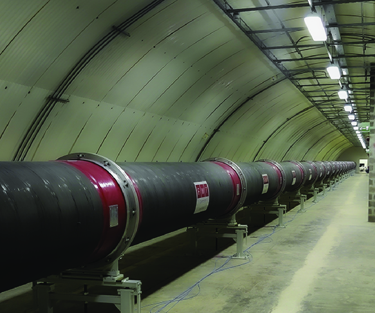
An experimental campaign was carried out at the Centre for International Cooperation in Long-Pipe Experiments (CICLoPE, see figure 1
a,b). The laboratory is realised inside a mountain to keep stable environmental conditions and to minimise background noise, while sound-absorbing material ensures minimal acoustic interference in the test section. The closed-loop facility comprises a 111.15 m-long circular pipe with a radius of $R = D/2 = 0.4505\,\rm m$
. The primary streamwise location for measurements (where the flow is fully developed) is at
$R = D/2 = 0.4505\,\rm m$
. The primary streamwise location for measurements (where the flow is fully developed) is at $x^\prime = 110.1\,\textrm { m} = 244.4R$
downstream of the pipe inlet. For the experiments reported, the pipe flow was operated at seven centreline velocities, with a maximum of
$x^\prime = 110.1\,\textrm { m} = 244.4R$
downstream of the pipe inlet. For the experiments reported, the pipe flow was operated at seven centreline velocities, with a maximum of $U_{{ CL}} = 44.60\,\textrm { m}\,{\rm s^-{^1}}$
(corresponding to
$U_{{ CL}} = 44.60\,\textrm { m}\,{\rm s^-{^1}}$
(corresponding to $Re_\tau \equiv U_\tau R/\nu = 47\,015$
). Test conditions are elaborated upon in § 2.3. For presenting results, a Cartesian coordinate system is adopted with its origin at the primary streamwise location for measurements (at the centre of sensor
$Re_\tau \equiv U_\tau R/\nu = 47\,015$
). Test conditions are elaborated upon in § 2.3. For presenting results, a Cartesian coordinate system is adopted with its origin at the primary streamwise location for measurements (at the centre of sensor $\mathcal{M}_1$
, indicated in figure 1
c). Here, the
$\mathcal{M}_1$
, indicated in figure 1
c). Here, the $x$
-axis denotes the streamwise direction (positive in the downstream direction) and the
$x$
-axis denotes the streamwise direction (positive in the downstream direction) and the $y$
-axis denotes the wall-normal direction (
$y$
-axis denotes the wall-normal direction ( $y = 0$
at the wall and positive towards the centreline of the pipe). A comprehensive description of all design details of the facility can be found in the literature (Talamelli et al. Reference Talamelli, Persiani, Fransson, Alfredsson, Johansson, Nagib, Rüedi, Sreenivasan and Monkewitz2009; Bellani & Talamelli Reference Bellani and Talamelli2016).
$y = 0$
at the wall and positive towards the centreline of the pipe). A comprehensive description of all design details of the facility can be found in the literature (Talamelli et al. Reference Talamelli, Persiani, Fransson, Alfredsson, Johansson, Nagib, Rüedi, Sreenivasan and Monkewitz2009; Bellani & Talamelli Reference Bellani and Talamelli2016).
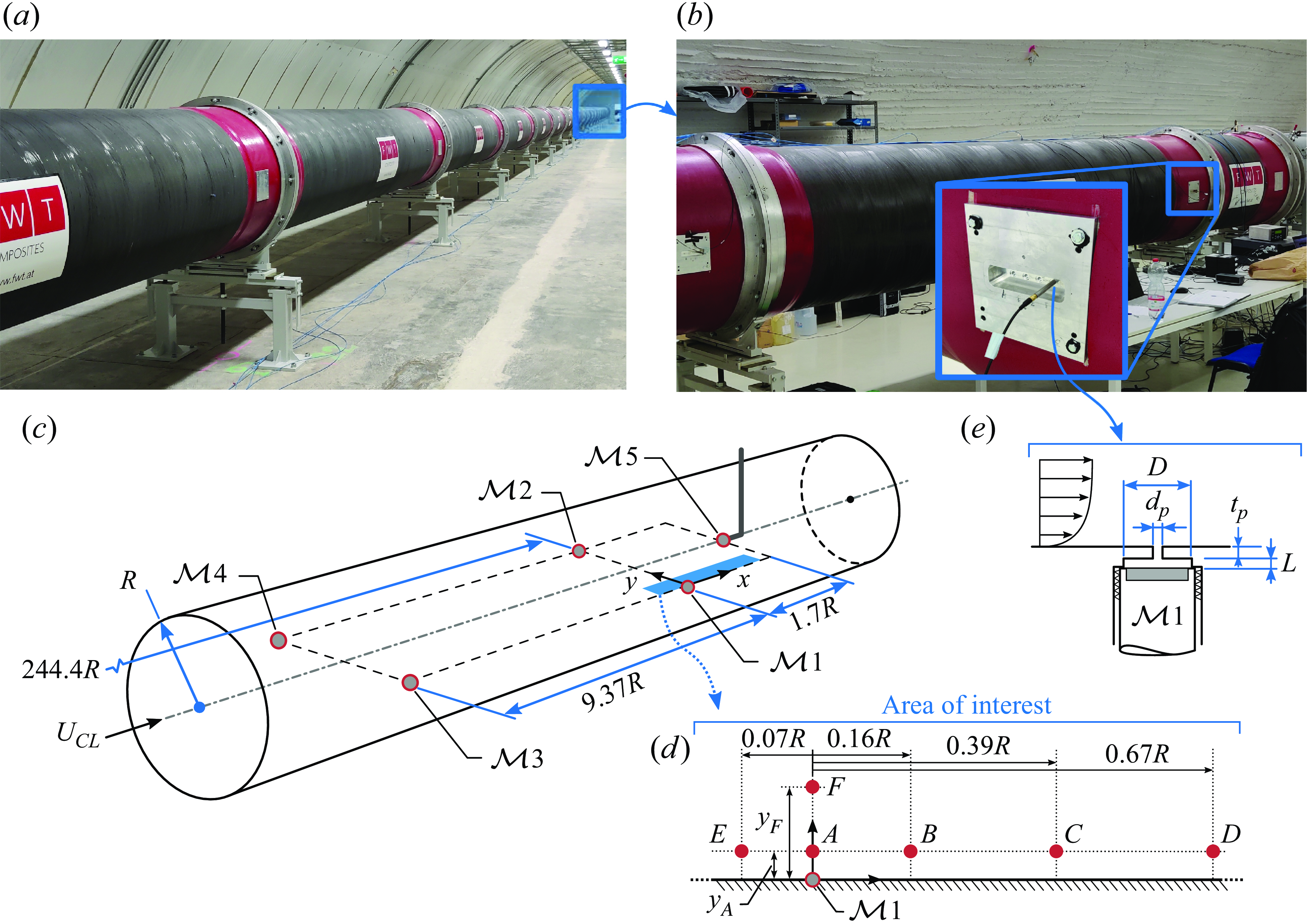
Figure 1. (a) Photograph of the CICLoPE laboratory, with (b) the test section at the downstream end of the long-pipe facility. (c) Schematic of the microphone sensor placement ( $\mathcal{M}1$
to
$\mathcal{M}1$
to $\mathcal{M}4$
were mounted in the pipe wall and
$\mathcal{M}4$
were mounted in the pipe wall and $\mathcal{M}5$
was mounted along the pipe centreline). (d) Illustration of the points in the area of interest where acquisitions with single-wire and x-wire probes were performed. (e) Schematic of the pinhole–sub-surface cavity, used to mount the microphones in the pipe wall.
$\mathcal{M}5$
was mounted along the pipe centreline). (d) Illustration of the points in the area of interest where acquisitions with single-wire and x-wire probes were performed. (e) Schematic of the pinhole–sub-surface cavity, used to mount the microphones in the pipe wall.
2.2. Measurement instrumentation
Time-resolved pressure sensors were integrated in the wall of the pipe, each within its own cavity communicating with the flow through a pinhole orifice. Figure 1(e) provides a schematic of the axisymmetric geometry of the pinhole and its corresponding sub-surface cavity, comprising a pinhole orifice diameter of ${d}_p = 0.3\,\rm mm$
, a pinhole depth of
${d}_p = 0.3\,\rm mm$
, a pinhole depth of $t_p = 1.1\,\rm mm$
, an effective cavity diameter of
$t_p = 1.1\,\rm mm$
, an effective cavity diameter of $D = 4.6\,\rm mm$
and a cavity length of
$D = 4.6\,\rm mm$
and a cavity length of $L = 0.2\,\rm mm$
. The size of the pinhole orifice ensures a sufficient spatial measurement resolution for the purpose of coherence analysis (§ 2.3). However, because of the sub-surface-cavity geometry, a Kelvin–Helmholtz resonance occurs. This resonance phenomenon was quantified by means of an acoustic characterisation experiment, following an identical procedure (in the exact same facility) as the one described by Baars et al. (Reference Baars, Dacome and Lee2024, pp. 30–32). Similar procedures can be found in other works (e.g. Gravante et al. Reference Gravante, Naguib, Wark and Nagib1998; Tsuji et al. Reference Tsuji, Fransson, Alfredsson and Johansson2007; Gibeau & Ghaemi Reference Gibeau and Ghaemi2021). In short, pressures at the orifice inlet (
$L = 0.2\,\rm mm$
. The size of the pinhole orifice ensures a sufficient spatial measurement resolution for the purpose of coherence analysis (§ 2.3). However, because of the sub-surface-cavity geometry, a Kelvin–Helmholtz resonance occurs. This resonance phenomenon was quantified by means of an acoustic characterisation experiment, following an identical procedure (in the exact same facility) as the one described by Baars et al. (Reference Baars, Dacome and Lee2024, pp. 30–32). Similar procedures can be found in other works (e.g. Gravante et al. Reference Gravante, Naguib, Wark and Nagib1998; Tsuji et al. Reference Tsuji, Fransson, Alfredsson and Johansson2007; Gibeau & Ghaemi Reference Gibeau and Ghaemi2021). In short, pressures at the orifice inlet ( $p_i$
) and within the cavity (
$p_i$
) and within the cavity ( $p_c$
) were measured simultaneously, in quiescent flow conditions, under a broadband acoustic excitation in an anechoic facility. A linear transfer kernel was constructed, relating cavity to inlet pressure in the frequency domain:
$p_c$
) were measured simultaneously, in quiescent flow conditions, under a broadband acoustic excitation in an anechoic facility. A linear transfer kernel was constructed, relating cavity to inlet pressure in the frequency domain: $H_r^{{ exp}} (f) = \langle \widetilde {P}_c(f) \widetilde {P}^*_i(f) \rangle / \langle \vert \widetilde {P}_i(f) \vert ^2 \rangle$
. Here, the angled brackets
$H_r^{{ exp}} (f) = \langle \widetilde {P}_c(f) \widetilde {P}^*_i(f) \rangle / \langle \vert \widetilde {P}_i(f) \vert ^2 \rangle$
. Here, the angled brackets $\langle \ldots \rangle$
indicate ensemble averaging, the
$\langle \ldots \rangle$
indicate ensemble averaging, the $*$
denotes the complex conjugate and capitalised variables with a tilde indicate the Fourier transformed quantity, e.g.
$*$
denotes the complex conjugate and capitalised variables with a tilde indicate the Fourier transformed quantity, e.g. $\widetilde {P}_c(f) = \mathcal{F} [p_c(t)]$
. Subsequently, a second-order model was fit to the gain of this transfer kernel and is denoted as
$\widetilde {P}_c(f) = \mathcal{F} [p_c(t)]$
. Subsequently, a second-order model was fit to the gain of this transfer kernel and is denoted as $\vert H_r(f)\vert$
. This procedure enabled the identification of the resonance frequency of the pinhole–sub-surface cavity at
$\vert H_r(f)\vert$
. This procedure enabled the identification of the resonance frequency of the pinhole–sub-surface cavity at $f_r = 4{}350\,\rm Hz$
. Implications of the resonance phenomenon on the wall-pressure measurements and coherence analyses are discussed later in § 3.
$f_r = 4{}350\,\rm Hz$
. Implications of the resonance phenomenon on the wall-pressure measurements and coherence analyses are discussed later in § 3.
Regarding the pressure sensors themselves, GRAS 46BE 1/4 in. CCP free-field microphones were employed. These have an adequate dynamic range (35–160 dB, with a reference pressure of $p_{{ ref}} = 20$ $\unicode{x03BC}$
Pa) with an accuracy of
$\unicode{x03BC}$
Pa) with an accuracy of $\pm 1$
dB within the range of 10 Hz to 40 kHz. Data were acquired with two NI9234 analogue-input boards, comprising a 24-bit A/D conversion resolution. A total of five microphones were employed (labelled
$\pm 1$
dB within the range of 10 Hz to 40 kHz. Data were acquired with two NI9234 analogue-input boards, comprising a 24-bit A/D conversion resolution. A total of five microphones were employed (labelled $\mathcal{M}1$
to
$\mathcal{M}1$
to $\mathcal{M}5$
in figure 1
c): four were integrated in the pipe for wall-pressure measurements (
$\mathcal{M}5$
in figure 1
c): four were integrated in the pipe for wall-pressure measurements ( $\mathcal{M}1$
to
$\mathcal{M}1$
to $\mathcal{M}4$
) and one was mounted on a streamlined holder along the pipe centreline for monitoring the acoustic noise of the facility (
$\mathcal{M}4$
) and one was mounted on a streamlined holder along the pipe centreline for monitoring the acoustic noise of the facility ( $\mathcal{M}5$
). Microphone
$\mathcal{M}5$
). Microphone $\mathcal{M}5$
was equipped with a GRAS RA0020 nose cone to reduce stagnation-driven turbulence pressure fluctuations on the otherwise flow-exposed diaphragm. The wall-mounted microphones were arranged in two streamwise pairs, separated by a distance of 4.22 m (
$\mathcal{M}5$
was equipped with a GRAS RA0020 nose cone to reduce stagnation-driven turbulence pressure fluctuations on the otherwise flow-exposed diaphragm. The wall-mounted microphones were arranged in two streamwise pairs, separated by a distance of 4.22 m ( $\Delta x = 9.37R$
). Microphones in one pair were located in azimuthally opposite positions to facilitate the removal of facility (acoustic) noise.
$\Delta x = 9.37R$
). Microphones in one pair were located in azimuthally opposite positions to facilitate the removal of facility (acoustic) noise.
Time series of streamwise velocity at two wall-normal locations in the logarithmic region ( $y_{A} = 0.011$
m
$y_{A} = 0.011$
m $= 0.025R$
and
$= 0.025R$
and $y_{F} = 0.061$
m
$y_{F} = 0.061$
m $= 0.135R$
), and at five streamwise locations (points
$= 0.135R$
), and at five streamwise locations (points $A$
to
$A$
to $E$
in figure 1
d), were acquired using hot-wire anemometry (HWA). Synchronised measurements were performed of all microphones’ signal at once, while velocity could only be measured at a single
$E$
in figure 1
d), were acquired using hot-wire anemometry (HWA). Synchronised measurements were performed of all microphones’ signal at once, while velocity could only be measured at a single $y$
-location for a given run. Each measurement was performed with an acquisition frequency of
$y$
-location for a given run. Each measurement was performed with an acquisition frequency of $f_s = 51.2\,\rm kHz$
, for an uninterrupted duration of
$f_s = 51.2\,\rm kHz$
, for an uninterrupted duration of $T_a = 480\,\rm s$
(relatively long time series were acquired to ensure sufficient convergence of the spectral statistics at the lowest frequencies of interest). A Dantec Streamline 90C10 CTA module was used, with a Dantec 55P15 single-wire boundary layer probe. Additionally, time series of the wall-normal velocity component were acquired using a Dantec 55P61 miniature x-wire probe at one point in the logarithmic region (point
$T_a = 480\,\rm s$
(relatively long time series were acquired to ensure sufficient convergence of the spectral statistics at the lowest frequencies of interest). A Dantec Streamline 90C10 CTA module was used, with a Dantec 55P15 single-wire boundary layer probe. Additionally, time series of the wall-normal velocity component were acquired using a Dantec 55P61 miniature x-wire probe at one point in the logarithmic region (point $A$
in figure 1
d). All Pt-plated tungsten wires of the single-wire and x-wire probes comprised sensing lengths of
$A$
in figure 1
d). All Pt-plated tungsten wires of the single-wire and x-wire probes comprised sensing lengths of $l_{{ hw}}=1.25\,\rm mm$
and nominal diameters of
$l_{{ hw}}=1.25\,\rm mm$
and nominal diameters of $d_{{ hw}}=5\,\unicode{x03BC}\rm m$
(thus,
$d_{{ hw}}=5\,\unicode{x03BC}\rm m$
(thus, $l_{{ hw}}/d_{{ hw}} \approx 250$
). Hot-wire probes were calibrated ex situ by employing a planar calibration jet. The single-wire probe was calibrated by fitting a fifth-order polynomial function to 11 calibration points of velocity versus measured voltage,
$l_{{ hw}}/d_{{ hw}} \approx 250$
). Hot-wire probes were calibrated ex situ by employing a planar calibration jet. The single-wire probe was calibrated by fitting a fifth-order polynomial function to 11 calibration points of velocity versus measured voltage, $U = f(E)$
. For the x-wire instead, seven velocity settings and 13 angular positions were set to generate a two-dimensional look-up table (Burattini & Antonia Reference Burattini and Antonia2004) relating the two velocity components to the measured voltages of each wire:
$U = f(E)$
. For the x-wire instead, seven velocity settings and 13 angular positions were set to generate a two-dimensional look-up table (Burattini & Antonia Reference Burattini and Antonia2004) relating the two velocity components to the measured voltages of each wire: $ (U_1,U_2) = f (E_1,E_2)$
. During the measurements, the probe was oriented in such a way that it measured the streamwise (
$ (U_1,U_2) = f (E_1,E_2)$
. During the measurements, the probe was oriented in such a way that it measured the streamwise ( $u$
) and wall-normal (
$u$
) and wall-normal ( $v$
) velocity components simultaneously. More details of similar HWA measurements in the CICLoPE facility can be found in the works by Örlü et al. (Reference Örlü, Fiorini, Segalini, Bellani, Talamelli and Alfredsson2017) and Zheng et al. (Reference Zheng2022).
$v$
) velocity components simultaneously. More details of similar HWA measurements in the CICLoPE facility can be found in the works by Örlü et al. (Reference Örlü, Fiorini, Segalini, Bellani, Talamelli and Alfredsson2017) and Zheng et al. (Reference Zheng2022).
2.3. Experimental conditions and measurement resolution
Seven experimental conditions were considered for measurements of the fluctuating wall-pressure and velocity in the CICLoPE long-pipe facility. Flow parameters of all test cases are reported in table 1. With the aid of a heat exchanger, the facility was operated at constant temperature and the angular velocities of the two co-axial fans were set to generate centreline velocities in the range $3.837\,\textrm { m}\,{\rm s^-{^1}} \leqslant U_{\textit{CL}} \leqslant 44.60\,\textrm { m}\,{\rm s^-{^1}}$
(measured with a Pitot-static probe). Corresponding values of the wall-shear stress,
$3.837\,\textrm { m}\,{\rm s^-{^1}} \leqslant U_{\textit{CL}} \leqslant 44.60\,\textrm { m}\,{\rm s^-{^1}}$
(measured with a Pitot-static probe). Corresponding values of the wall-shear stress, $\tau _w$
, were inferred from static pressure drop measurements (following Fiorini Reference Fiorini2017). Values for the air density were indirectly measured with the air flow temperature and barometric pressure, so that values for the friction velocity,
$\tau _w$
, were inferred from static pressure drop measurements (following Fiorini Reference Fiorini2017). Values for the air density were indirectly measured with the air flow temperature and barometric pressure, so that values for the friction velocity, $U_\tau$
, could be computed. For the experiments reported in this work, friction Reynolds numbers were in the range
$U_\tau$
, could be computed. For the experiments reported in this work, friction Reynolds numbers were in the range $4794 \lesssim Re_\tau \lesssim 47\,015$
.
$4794 \lesssim Re_\tau \lesssim 47\,015$
.
Table 1. Flow parameters corresponding to the seven test conditions in the CICLoPE long-pipe facility, alongside non-dimensional parameters of the instrumentation’s geometry and acquisition details.
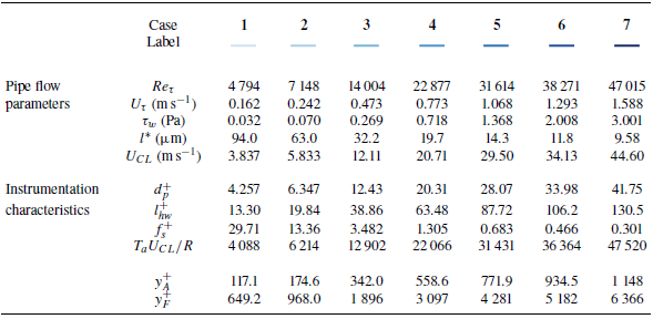
Spatial and temporal resolutions need to be considered for both the fluctuating wall-pressure and velocity measurements. For the measurement of wall-pressure, the pinhole orifice diameter dictates the spatial resolution, while for the measurement of velocity, the hot-wire sensing length is determining the spatial resolution. The temporal resolution was limited by the acquisition frequency. All three parameters relevant for the measurement resolutions ( $d_p$
,
$d_p$
, $l_{hw}$
and
$l_{hw}$
and $f_s$
) are listed in table 1 after normalisation with the viscous scales.
$f_s$
) are listed in table 1 after normalisation with the viscous scales.
For fully resolved wall-pressure measurements, the pinhole orifice diameter must be $d_p^+ \lt 20$
(Gravante et al. Reference Gravante, Naguib, Wark and Nagib1998). Hence, the pinhole diameter is not sufficiently small to claim fully resolved wall-pressure measurements for test cases 4 to 7 (the relatively large values of
$d_p^+ \lt 20$
(Gravante et al. Reference Gravante, Naguib, Wark and Nagib1998). Hence, the pinhole diameter is not sufficiently small to claim fully resolved wall-pressure measurements for test cases 4 to 7 (the relatively large values of $d_p^+$
result in an attenuation of small-scale energy). However, this work does not revolve around conducting fully resolved measurements, but rather focuses on the correlation between velocity fluctuations in the logarithmic region and wall-pressure. As reviewed in § 1, the scales of interest for the correlation analyses reside at streamwise wavelengths of
$d_p^+$
result in an attenuation of small-scale energy). However, this work does not revolve around conducting fully resolved measurements, but rather focuses on the correlation between velocity fluctuations in the logarithmic region and wall-pressure. As reviewed in § 1, the scales of interest for the correlation analyses reside at streamwise wavelengths of $\lambda _x/y \gtrsim 3$
(when considering
$\lambda _x/y \gtrsim 3$
(when considering $u$
fluctuations) and
$u$
fluctuations) and $\lambda _x/y \gtrsim 1$
(when considering
$\lambda _x/y \gtrsim 1$
(when considering $v$
fluctuations). Smaller streamwise scales in both the pressure and pressure-squared time series are not relevant, as they do not correlate with the ones in the turbulent velocity signals. Consequently, for all
$v$
fluctuations). Smaller streamwise scales in both the pressure and pressure-squared time series are not relevant, as they do not correlate with the ones in the turbulent velocity signals. Consequently, for all $Re_\tau$
test cases, a minimum streamwise wavelength that needs to be resolved for the coherence analyses is given by
$Re_\tau$
test cases, a minimum streamwise wavelength that needs to be resolved for the coherence analyses is given by $\lambda _{x,{res}}/y_A = 1$
(recall that
$\lambda _{x,{res}}/y_A = 1$
(recall that $y_A$
is the lowest wall-normal position being considered), resulting in a streamwise wavelength of
$y_A$
is the lowest wall-normal position being considered), resulting in a streamwise wavelength of $\lambda _{x,{res}} = y_A = 11\,\rm mm$
. The pinhole orifice diameter of
$\lambda _{x,{res}} = y_A = 11\,\rm mm$
. The pinhole orifice diameter of ${d}_p = 0.3\,\rm mm$
is a factor of 36.6 smaller and, thus, sufficient for capturing the streamwise wavelengths of interest.
${d}_p = 0.3\,\rm mm$
is a factor of 36.6 smaller and, thus, sufficient for capturing the streamwise wavelengths of interest.
When considering the spatial resolution of the HWA measurements, a similar reasoning can be applied. Statistically, the velocity structures of relevance to the wall-pressure–velocity correlations adhere to a self-similar scaling in all three dimensions. Baidya et al. (Reference Baidya2019) showed that the aspect ratio of coherent velocity structures is 7 : 1, in terms of their characteristic streamwise-to-spanwise length scales. Hence, the smallest structures of relevance have spanwise wavelengths of $\lambda _{z,{res}} = \lambda _{x,{res}}/7 \approx 1.6\,\rm mm$
. For the HWA measurements with the x-wire probe, the spanwise separation between both sensing wires is
$\lambda _{z,{res}} = \lambda _{x,{res}}/7 \approx 1.6\,\rm mm$
. For the HWA measurements with the x-wire probe, the spanwise separation between both sensing wires is ${\sim} 1.0\,\rm mm$
, which is sufficient to resolve the scales of interest. In the
${\sim} 1.0\,\rm mm$
, which is sufficient to resolve the scales of interest. In the $y$
-direction, the sensing length of the x-wire probe is also adequate, given the strong wall-normal coherence of the velocity structures. For the single-wire probe, its spanwise sensing length of
$y$
-direction, the sensing length of the x-wire probe is also adequate, given the strong wall-normal coherence of the velocity structures. For the single-wire probe, its spanwise sensing length of $l_{{ HW}} = 1.25\,\rm mm$
is more than sufficient given that the
$l_{{ HW}} = 1.25\,\rm mm$
is more than sufficient given that the $u$
fluctuations of interest are three times larger than the
$u$
fluctuations of interest are three times larger than the $v$
fluctuations of interest.
$v$
fluctuations of interest.
Regarding the temporal measurement resolution, this is set by the data acquisition rate. For the highest $Re_\tau$
test case (number 7), the acquisition time step is largest in terms of viscous time scales and equals
$Re_\tau$
test case (number 7), the acquisition time step is largest in terms of viscous time scales and equals $\Delta T^+ = 1/f_s^+ \approx 3.3$
. Even though Hutchins et al. (Reference Hutchins, Nickels, Marusic and Chong2009) indicate a required time step
$\Delta T^+ = 1/f_s^+ \approx 3.3$
. Even though Hutchins et al. (Reference Hutchins, Nickels, Marusic and Chong2009) indicate a required time step $\Delta T^+$
of unity or less for fully resolved measurements, the current acquisition rate is more than sufficient given the interest in much lower frequencies (larger spatial scales) than those corresponding to the dissipative regime.
$\Delta T^+$
of unity or less for fully resolved measurements, the current acquisition rate is more than sufficient given the interest in much lower frequencies (larger spatial scales) than those corresponding to the dissipative regime.
2.4. Post-processing of wall-pressure signals
Even though the CICLoPE laboratory has been designed to minimise noise in the test section, the facility is non-anechoic and acoustic pressure fluctuations do contaminate the measured wall-pressure signals. A superposition of facility noise onto the time series of the hydrodynamic wall-pressure affects the wall-pressure statistics. Furthermore, the correlation analyses are affected since, by construction, facility noise and velocity fluctuations are uncorrelated. Therefore, a normalised correlation (with the additive facility noise present) is lower than the true value (Saccenti, Hendriks & Smilde Reference Saccenti, Hendriks and Smilde2020).
Given the need to remove facility noise, a post-processing procedure is applied based on harmonic proper orthogonal decomposition (hPOD, reviewed by Tinney, Shipman & Panickar Reference Tinney, Shipman and Panickar2020). First, POD kernels are constructed from cross-spectral densities of, in this case, the various pressure signals. Then, the solution of an eigenvalue problem yields the frequency-dependent mode shapes and eigenvalues. By only retaining modes of the measured pressure time series, in which the spectral signature of facility noise is absent, hydrodynamic wall-pressure signals are inferred. All details of the noise-removal procedure are described in Appendix A.
3. Wall-pressure statistics in the CICLoPE facility
Statistics of the wall-pressure fluctuations are presented to demonstrate the validity of our data for the correlation analyses presented in §§ 4 and 5.
Probability density functions (p.d.f.s) of the wall-pressure time series are shown in figures 2(a) and 2(b), with a linear and logarithmic scale on the ordinate axes, respectively. For both figures, the amplitude axes are scaled with the wall-pressure intensity (root-mean-square), denoted as $p^\prime _w$
. Superimposed are several p.d.f.s from the literature: a p.d.f. corresponding to an atmospheric boundary layer flow at
$p^\prime _w$
. Superimposed are several p.d.f.s from the literature: a p.d.f. corresponding to an atmospheric boundary layer flow at $Re_\tau \approx 1 \times 10^6 \pm 2\times 10^5$
(Klewicki et al. Reference Klewicki, Priyadarshana and Metzger2008) and a band representing the spread of p.d.f.s corresponding to zero-pressure-gradient TBL flow at
$Re_\tau \approx 1 \times 10^6 \pm 2\times 10^5$
(Klewicki et al. Reference Klewicki, Priyadarshana and Metzger2008) and a band representing the spread of p.d.f.s corresponding to zero-pressure-gradient TBL flow at $1313 \lesssim Re_\tau \lesssim 3826$
(Tsuji et al. Reference Tsuji, Fransson, Alfredsson and Johansson2007). All p.d.f.s of the current datasets show negligible disparity between the test cases and are consistent with the distributions from the literature. Minor deviations appear in the tails of the p.d.f.s (figure 2
b), yet comparable with the degree of deviation in the work by Tsuji et al. (Reference Tsuji, Fransson, Alfredsson and Johansson2007) and without a noticeable monotonic trend with an increase in
$1313 \lesssim Re_\tau \lesssim 3826$
(Tsuji et al. Reference Tsuji, Fransson, Alfredsson and Johansson2007). All p.d.f.s of the current datasets show negligible disparity between the test cases and are consistent with the distributions from the literature. Minor deviations appear in the tails of the p.d.f.s (figure 2
b), yet comparable with the degree of deviation in the work by Tsuji et al. (Reference Tsuji, Fransson, Alfredsson and Johansson2007) and without a noticeable monotonic trend with an increase in $Re_\tau$
.
$Re_\tau$
.
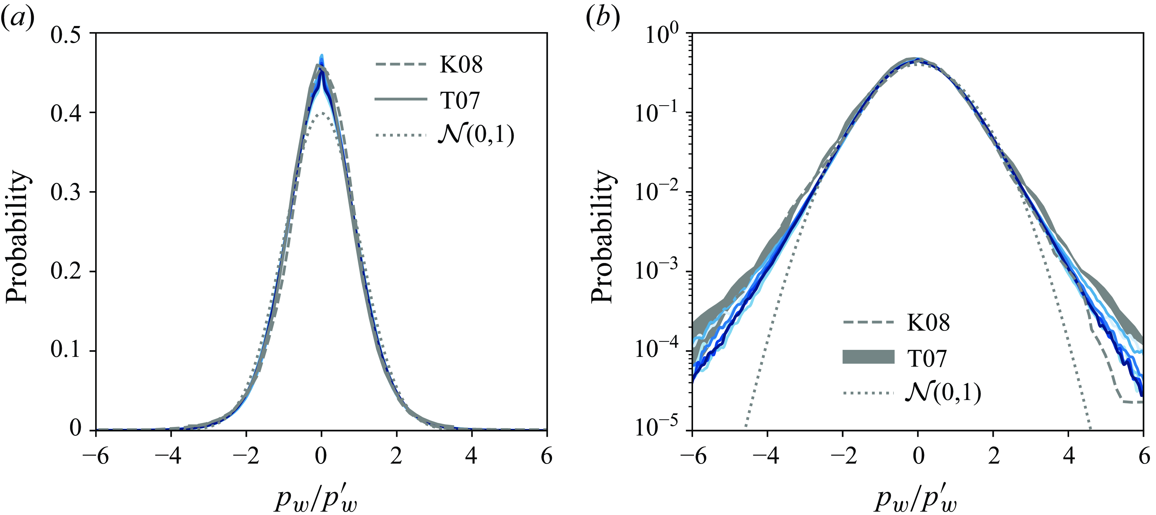
Figure 2. Probability density functions of the wall-pressure fluctuations in the CICLoPE facility for all $Re_\tau$
test cases considered (see table 1). Current data are compared with a p.d.f. obtained from atmospheric boundary layer data at
$Re_\tau$
test cases considered (see table 1). Current data are compared with a p.d.f. obtained from atmospheric boundary layer data at $Re_\tau \approx 10^6$
(Klewicki et al. Reference Klewicki, Priyadarshana and Metzger2008), label K08), and a band representing the spread of p.d.f.s obtained from zero-pressure-gradient TBL data at
$Re_\tau \approx 10^6$
(Klewicki et al. Reference Klewicki, Priyadarshana and Metzger2008), label K08), and a band representing the spread of p.d.f.s obtained from zero-pressure-gradient TBL data at $1{}313 \lesssim Re_\tau \lesssim 3{}826$
(Tsuji et al. Reference Tsuji, Fransson, Alfredsson and Johansson2007, label T07). A standard
$1{}313 \lesssim Re_\tau \lesssim 3{}826$
(Tsuji et al. Reference Tsuji, Fransson, Alfredsson and Johansson2007, label T07). A standard $\mathcal{N}(0,1)$
Gaussian distribution is added for reference. Probability density functions are plotted with (a) a linear scale and (b) a logarithmic scale on the ordinate axes. Data employed for plotting panels (a) and (b) are available in the supplementary material.
$\mathcal{N}(0,1)$
Gaussian distribution is added for reference. Probability density functions are plotted with (a) a linear scale and (b) a logarithmic scale on the ordinate axes. Data employed for plotting panels (a) and (b) are available in the supplementary material.

Figure 3. (a,b) Pre-multiplied energy spectra of wall-pressure fluctuations, for all $Re_\tau$
test cases considered (an increase in colour intensity corresponds to an increase in
$Re_\tau$
test cases considered (an increase in colour intensity corresponds to an increase in $Re_\tau$
following test cases
$Re_\tau$
following test cases $1\rightarrow 7$
, listed in table 1), as a function of (a) the viscous scaled wavelength and (b) the outer-scaled wavelength. Note that the temporal spectra are plotted as spatial spectra by converting frequency into wavelength, using
$1\rightarrow 7$
, listed in table 1), as a function of (a) the viscous scaled wavelength and (b) the outer-scaled wavelength. Note that the temporal spectra are plotted as spatial spectra by converting frequency into wavelength, using $\lambda _x \equiv U_c/f$
with
$\lambda _x \equiv U_c/f$
with $U_c^+ = 10$
. Vertical dashed lines in panel (b) indicate the minimum wavelength in our dataset for which wall-pressure–velocity correlations become appreciable when considering
$U_c^+ = 10$
. Vertical dashed lines in panel (b) indicate the minimum wavelength in our dataset for which wall-pressure–velocity correlations become appreciable when considering $u$
fluctuations (
$u$
fluctuations ( $\lambda _x/y_A = 3$
) and
$\lambda _x/y_A = 3$
) and $v$
fluctuations (
$v$
fluctuations ( $\lambda _x/y_A = 1$
). (c,d) Gain of transfer kernel
$\lambda _x/y_A = 1$
). (c,d) Gain of transfer kernel $H_r$
that characterises the pinhole–sub-surface cavity as described in § 2.2, including in (c) the gain of the raw kernel,
$H_r$
that characterises the pinhole–sub-surface cavity as described in § 2.2, including in (c) the gain of the raw kernel, $H_r^{\textit{exp}}$
(light grey line). Data employed for plotting panels (a) and (b) are available in the supplementary material.
$H_r^{\textit{exp}}$
(light grey line). Data employed for plotting panels (a) and (b) are available in the supplementary material.
Pre-multiplied energy spectra of wall-pressure fluctuations are shown in figures 3(a) and 3(b) for all values of $Re_\tau$
, with an inner-scaled and outer-scaled streamwise wavelength on the abscissa, respectively. Here, the streamwise wavelength is obtained by applying Taylor’s hypothesis:
$Re_\tau$
, with an inner-scaled and outer-scaled streamwise wavelength on the abscissa, respectively. Here, the streamwise wavelength is obtained by applying Taylor’s hypothesis: $\lambda _x \equiv U_c/f$
, where
$\lambda _x \equiv U_c/f$
, where $f$
is the frequency and
$f$
is the frequency and $U_c$
is the convection velocity taken as
$U_c$
is the convection velocity taken as $U_c^+ = 10$
. Despite the convection velocity of the wall-pressure field being scale-dependent (e.g. Luhar, Sharma & McKeon Reference Luhar, Sharma and McKeon2014) and the temporal-to-spatial conversion of near-wall fluctuations in velocity/pressure not abiding by Taylor’s hypothesis (Dennis & Nickels Reference Dennis and Nickels2008; del Á lamo & Jiménez Reference del Álamo and Jiménez2009), the conversion is kept equal across all test cases. In essence, we compare temporal spectra (since
$U_c^+ = 10$
. Despite the convection velocity of the wall-pressure field being scale-dependent (e.g. Luhar, Sharma & McKeon Reference Luhar, Sharma and McKeon2014) and the temporal-to-spatial conversion of near-wall fluctuations in velocity/pressure not abiding by Taylor’s hypothesis (Dennis & Nickels Reference Dennis and Nickels2008; del Á lamo & Jiménez Reference del Álamo and Jiménez2009), the conversion is kept equal across all test cases. In essence, we compare temporal spectra (since $\lambda _x^+ = 10U^2_\tau /\nu /f = 10/f^+$
). Still the temporal-to-spatial conversion was applied because §§ 4 and 5 consider all coherence spectra as a function of wavelength for ease of comparison to the only data available (those from spatial DNS of turbulent channel flow).
$\lambda _x^+ = 10U^2_\tau /\nu /f = 10/f^+$
). Still the temporal-to-spatial conversion was applied because §§ 4 and 5 consider all coherence spectra as a function of wavelength for ease of comparison to the only data available (those from spatial DNS of turbulent channel flow).
Before commenting on the wall-pressure spectra, note that figures 3(c) and 3(d) present the gain of the transfer kernel that characterises the pinhole–sub-surface cavity (described in § 2.2). Because the transfer kernel is a function of frequency and the frequency-to-wavelength conversion includes the friction velocity of each test case, seven identical kernels are shown (but shifted along $\lambda _x$
). For reference, the raw experimental kernel,
$\lambda _x$
). For reference, the raw experimental kernel, $H_r^{{ exp}}$
, is shown in figure 3(c) for the highest
$H_r^{{ exp}}$
, is shown in figure 3(c) for the highest $Re_\tau$
test case with a thick grey line, while the other kernels correspond to the fitted kernel of the second-order model,
$Re_\tau$
test case with a thick grey line, while the other kernels correspond to the fitted kernel of the second-order model, $H_r$
. Noticeably, resonance occurs at scales where the wall-pressure spectra are energetic. It is thus necessary to correct the spectra for the amplification/attenuation effect. Current wall-pressure spectra were corrected before plotting, by dividing the spectra with the frequency-dependent model kernel (
$H_r$
. Noticeably, resonance occurs at scales where the wall-pressure spectra are energetic. It is thus necessary to correct the spectra for the amplification/attenuation effect. Current wall-pressure spectra were corrected before plotting, by dividing the spectra with the frequency-dependent model kernel ( $\phi _{pp}(f) = \phi _{pp,f}(f)/\vert H_r(f)\vert ^2$
, with
$\phi _{pp}(f) = \phi _{pp,f}(f)/\vert H_r(f)\vert ^2$
, with $\phi _{pp,f}$
being the spectrum after removing facility noise from the raw measurements of wall-pressure following Appendix A). The resonance-correction works theoretically, but practically the kernel (which was found with the aid of a flow-off experiment) changes when wall-bounded turbulence grazes the pinhole orifice (see Dacome et al. Reference Dacome, Mörsch, Kotsonis and Baars2024b
), making the correction imperfect. In practice, this results in an erroneous ‘wiggle’ in various spectra and is most noticeable in the spectrum of test case 7.
$\phi _{pp,f}$
being the spectrum after removing facility noise from the raw measurements of wall-pressure following Appendix A). The resonance-correction works theoretically, but practically the kernel (which was found with the aid of a flow-off experiment) changes when wall-bounded turbulence grazes the pinhole orifice (see Dacome et al. Reference Dacome, Mörsch, Kotsonis and Baars2024b
), making the correction imperfect. In practice, this results in an erroneous ‘wiggle’ in various spectra and is most noticeable in the spectrum of test case 7.
Close inspection of the wall-pressure spectra reveals expected Reynolds-number trends. At first, the location of the inner-spectral peak at $\lambda _{x,p}^+ \approx 250$
(figure 3
a) agrees well with previous findings (Farabee & Casarella Reference Farabee and Casarella1991; Tsuji et al. Reference Tsuji, Fransson, Alfredsson and Johansson2007; Klewicki et al. Reference Klewicki, Priyadarshana and Metzger2008; Panton et al. Reference Panton, Lee and Moser2017). A slight increase in the inner-spectral peak magnitude, with an increase in
$\lambda _{x,p}^+ \approx 250$
(figure 3
a) agrees well with previous findings (Farabee & Casarella Reference Farabee and Casarella1991; Tsuji et al. Reference Tsuji, Fransson, Alfredsson and Johansson2007; Klewicki et al. Reference Klewicki, Priyadarshana and Metzger2008; Panton et al. Reference Panton, Lee and Moser2017). A slight increase in the inner-spectral peak magnitude, with an increase in $Re_\tau$
, is also noticeable for test cases 4 to 7 (expected per the trends in Tsuji et al. Reference Tsuji, Fransson, Alfredsson and Johansson2007; Panton et al. Reference Panton, Lee and Moser2017; Yu et al. Reference Yu, Ceci and Pirozzoli2022). The large-scale energy content also progressively increases with
$Re_\tau$
, is also noticeable for test cases 4 to 7 (expected per the trends in Tsuji et al. Reference Tsuji, Fransson, Alfredsson and Johansson2007; Panton et al. Reference Panton, Lee and Moser2017; Yu et al. Reference Yu, Ceci and Pirozzoli2022). The large-scale energy content also progressively increases with $Re_\tau$
and exhibits a collapse in outer-scaling, for the range
$Re_\tau$
and exhibits a collapse in outer-scaling, for the range $\lambda _x/R \gtrsim 0.2$
(figure 3
b). This trend is in line with the findings reported in DNS studies at lower
$\lambda _x/R \gtrsim 0.2$
(figure 3
b). This trend is in line with the findings reported in DNS studies at lower $Re_\tau$
(Panton et al. Reference Panton, Lee and Moser2017; Yu et al. Reference Yu, Ceci and Pirozzoli2022). It also conforms to the work by Deshpande et al. (Reference Deshpande, Vinuesa, Klewicki and Marusic2025), who reason that the intermediate and large scales of the wall-pressure spectra grow with
$Re_\tau$
(Panton et al. Reference Panton, Lee and Moser2017; Yu et al. Reference Yu, Ceci and Pirozzoli2022). It also conforms to the work by Deshpande et al. (Reference Deshpande, Vinuesa, Klewicki and Marusic2025), who reason that the intermediate and large scales of the wall-pressure spectra grow with $Re_\tau$
due to the contributions of both the active and inactive motions in the grazing flow. Spectra corresponding to test cases 1 and 2 are outliers in that their broadband peak-magnitudes are relatively high. We postulate that this is due to an incomplete removal of facility noise, as any remaining signature of facility noise is more pronounced in the spectra of lower
$Re_\tau$
due to the contributions of both the active and inactive motions in the grazing flow. Spectra corresponding to test cases 1 and 2 are outliers in that their broadband peak-magnitudes are relatively high. We postulate that this is due to an incomplete removal of facility noise, as any remaining signature of facility noise is more pronounced in the spectra of lower $Re_\tau$
test cases. That is, the degree of facility noise was quantified with a signal-to-noise ratio (SNR), defined as the intensity ratio of turbulence-induced wall-pressure fluctuations, relative to those induced by facility noise:
$Re_\tau$
test cases. That is, the degree of facility noise was quantified with a signal-to-noise ratio (SNR), defined as the intensity ratio of turbulence-induced wall-pressure fluctuations, relative to those induced by facility noise: $ { SNR} = p^\prime _w/(p^\prime _{w,r} - p^\prime _w)$
. Here,
$ { SNR} = p^\prime _w/(p^\prime _{w,r} - p^\prime _w)$
. Here, $p^\prime _{w,r}$
is the pressure intensity (root-mean-square) of the raw, measured wall-pressure. SNRs in our dataset increase monotonically with
$p^\prime _{w,r}$
is the pressure intensity (root-mean-square) of the raw, measured wall-pressure. SNRs in our dataset increase monotonically with $Re_\tau$
, in the interval
$Re_\tau$
, in the interval $0.08 \leqslant { SNR} \leqslant 0.25$
. Additive facility noise is thus more noticeable in the spectra at lower
$0.08 \leqslant { SNR} \leqslant 0.25$
. Additive facility noise is thus more noticeable in the spectra at lower $Re_\tau$
. For the remainder of the paper, it is important to recall from § 2.3 that for the correlation analysis, the scales of interest reside at streamwise wavelengths beyond
$Re_\tau$
. For the remainder of the paper, it is important to recall from § 2.3 that for the correlation analysis, the scales of interest reside at streamwise wavelengths beyond $\lambda _x/y \approx 3$
(when considering
$\lambda _x/y \approx 3$
(when considering $u$
fluctuations) and
$u$
fluctuations) and $\lambda _x/y \approx 1$
(when considering
$\lambda _x/y \approx 1$
(when considering $v$
fluctuations). Both of these limits are indicated in figure 3(b); within the scale-range of interest, the spectra are not affected by the kernel-correction and only the two lowest test cases seem affected by additive (acoustics-driven) noise.
$v$
fluctuations). Both of these limits are indicated in figure 3(b); within the scale-range of interest, the spectra are not affected by the kernel-correction and only the two lowest test cases seem affected by additive (acoustics-driven) noise.

Figure 4. Wall-pressure intensity inferred from integrating the wall-pressure spectra. Current results are compared with several datasets available from the literature. Data are taken from the DNS studies of Panton et al. (Reference Panton, Lee and Moser2017) (P17-DNS, $\bullet$
, ZPG-TBL), Choi & Moin (Reference Choi and Moin1990) (CM90-DNS,
$\bullet$
, ZPG-TBL), Choi & Moin (Reference Choi and Moin1990) (CM90-DNS, $\blacktriangledown$
, TCF) and Yu et al. (Reference Yu, Ceci and Pirozzoli2022) (YU-DNS,
$\blacktriangledown$
, TCF) and Yu et al. (Reference Yu, Ceci and Pirozzoli2022) (YU-DNS, $\blacksquare$
, pipe flow). Furthermore, data are collected from experimental studies of ZPG-TBL flows: Blake (Reference Blake1970) (B70,
$\blacksquare$
, pipe flow). Furthermore, data are collected from experimental studies of ZPG-TBL flows: Blake (Reference Blake1970) (B70, $\triangle$
), Bull & Thomas (Reference Bull and Thomas1976) (BT76,
$\triangle$
), Bull & Thomas (Reference Bull and Thomas1976) (BT76, $\triangleleft$
), Farabee & Casarella (Reference Farabee and Casarella1991) (FC91,
$\triangleleft$
), Farabee & Casarella (Reference Farabee and Casarella1991) (FC91, $\triangleright$
), Horne (Reference Horne1989) (H89,
$\triangleright$
), Horne (Reference Horne1989) (H89, $\square$
), Klewicki et al. (Reference Klewicki, Priyadarshana and Metzger2008) (K08,
$\square$
), Klewicki et al. (Reference Klewicki, Priyadarshana and Metzger2008) (K08,
![]() ), McGrath & Simpson (Reference McGrath and Simpson1987) (MS87,
), McGrath & Simpson (Reference McGrath and Simpson1987) (MS87,
![]() ), Schewe (Reference Schewe1983) (S83,
), Schewe (Reference Schewe1983) (S83,
![]() ) and Tsuji et al. (Reference Tsuji, Fransson, Alfredsson and Johansson2007) (T07,
) and Tsuji et al. (Reference Tsuji, Fransson, Alfredsson and Johansson2007) (T07, $\circ$
), and of experimental studies of pipe flows: Lauchle & Daniels (Reference Lauchle and Daniels1987) (LD87,
$\circ$
), and of experimental studies of pipe flows: Lauchle & Daniels (Reference Lauchle and Daniels1987) (LD87,
![]() ) and Morrison (Reference Morrison2007) (M07,
) and Morrison (Reference Morrison2007) (M07,
![]() ). Solid and dashed lines are the formulations presented by Klewicki et al. (Reference Klewicki, Priyadarshana and Metzger2008), in which the pressure variance increases logarithmically with increasing
). Solid and dashed lines are the formulations presented by Klewicki et al. (Reference Klewicki, Priyadarshana and Metzger2008), in which the pressure variance increases logarithmically with increasing $Re_\tau$
. Data employed for plotting the wall-pressure intensity corresponding to the present work are available in the supplementary material.
$Re_\tau$
. Data employed for plotting the wall-pressure intensity corresponding to the present work are available in the supplementary material.
As a final wall-pressure statistic, we consider the wall-pressure intensities, resulting from the integration of the energy spectra. Here, the root-mean-square intensity is considered and inner-normalised following $p^{\prime +}_w = p^{\prime }_w/\tau _w$
. Wall-pressure intensities are plotted in figure 4 and compared with a variety of datasets from the literature. Data from channel flow DNS are added (Panton et al. Reference Panton, Lee and Moser2017), together with the various datasets assembled by Klewicki et al. (Reference Klewicki, Priyadarshana and Metzger2008) (and named in the caption) that include both numerical and experimental studies, comprising zero-pressure-gradient turbulent boundary layer (ZPG-TBL), turbulent channel (TCF) and pipe flows. Our current data confirm the trend of increasing pressure intensity with
$p^{\prime +}_w = p^{\prime }_w/\tau _w$
. Wall-pressure intensities are plotted in figure 4 and compared with a variety of datasets from the literature. Data from channel flow DNS are added (Panton et al. Reference Panton, Lee and Moser2017), together with the various datasets assembled by Klewicki et al. (Reference Klewicki, Priyadarshana and Metzger2008) (and named in the caption) that include both numerical and experimental studies, comprising zero-pressure-gradient turbulent boundary layer (ZPG-TBL), turbulent channel (TCF) and pipe flows. Our current data confirm the trend of increasing pressure intensity with $Re_\tau$
and closely follow the empirical relation of Klewicki et al. (Reference Klewicki, Priyadarshana and Metzger2008). Only the data point of test case 1 (at
$Re_\tau$
and closely follow the empirical relation of Klewicki et al. (Reference Klewicki, Priyadarshana and Metzger2008). Only the data point of test case 1 (at $Re_\tau \approx 4{}794$
) is an outlier, which is ascribed to the imperfect facility noise-filtering causing an overestimation of the wall-pressure intensity.
$Re_\tau \approx 4{}794$
) is an outlier, which is ascribed to the imperfect facility noise-filtering causing an overestimation of the wall-pressure intensity.
4. Coherence between streamwise velocity and wall-pressure fluctuations
To analyse the scale-dependent coupling between the fluctuations in streamwise velocity ( $u$
) and wall-pressure (
$u$
) and wall-pressure ( $p_w$
), the linear coherence spectrum (LCS) is employed. The LCS describes the stochastic coupling, on a per-scale basis, as the degree of phase-consistency. The LCS is defined as the magnitude-squared of the cross-spectrum between
$p_w$
), the linear coherence spectrum (LCS) is employed. The LCS describes the stochastic coupling, on a per-scale basis, as the degree of phase-consistency. The LCS is defined as the magnitude-squared of the cross-spectrum between $u$
and
$u$
and $p_w$
, normalised with the two auto-spectra of
$p_w$
, normalised with the two auto-spectra of $u$
and
$u$
and $p_w$
:
$p_w$
:
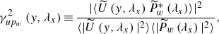 \begin{equation} \gamma _{up_w}^2\left (y,\lambda _x\right) \equiv \frac {\vert \langle \widetilde {U}\left (y,\lambda _x\right) \widetilde {P}^*_w\left (\lambda _x\right) \rangle \vert ^2}{\langle \vert \widetilde {U}\left (y,\lambda _x\right) \vert ^2 \rangle \langle \vert \widetilde {P}_w\left (\lambda _x\right)\vert ^2 \rangle }, \end{equation}
where the angled brackets $\langle \ldots \rangle$
indicate ensemble averaging, the
$\langle \ldots \rangle$
indicate ensemble averaging, the $*$
denotes the complex conjugate and capitalised variables with a tilde indicate the Fourier transformed quantity, e.g.
$*$
denotes the complex conjugate and capitalised variables with a tilde indicate the Fourier transformed quantity, e.g. $\widetilde {P}_w(f) = \mathcal{F} [p_w(t)]$
. Because in the remainder of the manuscript we present scale-dependent data as a function of streamwise wavelength, the argument in (4.1) is taken as
$\widetilde {P}_w(f) = \mathcal{F} [p_w(t)]$
. Because in the remainder of the manuscript we present scale-dependent data as a function of streamwise wavelength, the argument in (4.1) is taken as $\lambda _x$
and is, as for the energy spectra in § 3, obtained by applying Taylor’s hypothesis:
$\lambda _x$
and is, as for the energy spectra in § 3, obtained by applying Taylor’s hypothesis: $\lambda _x \equiv U_c/f$
, with
$\lambda _x \equiv U_c/f$
, with $U_c^+ = 10$
.
$U_c^+ = 10$
.
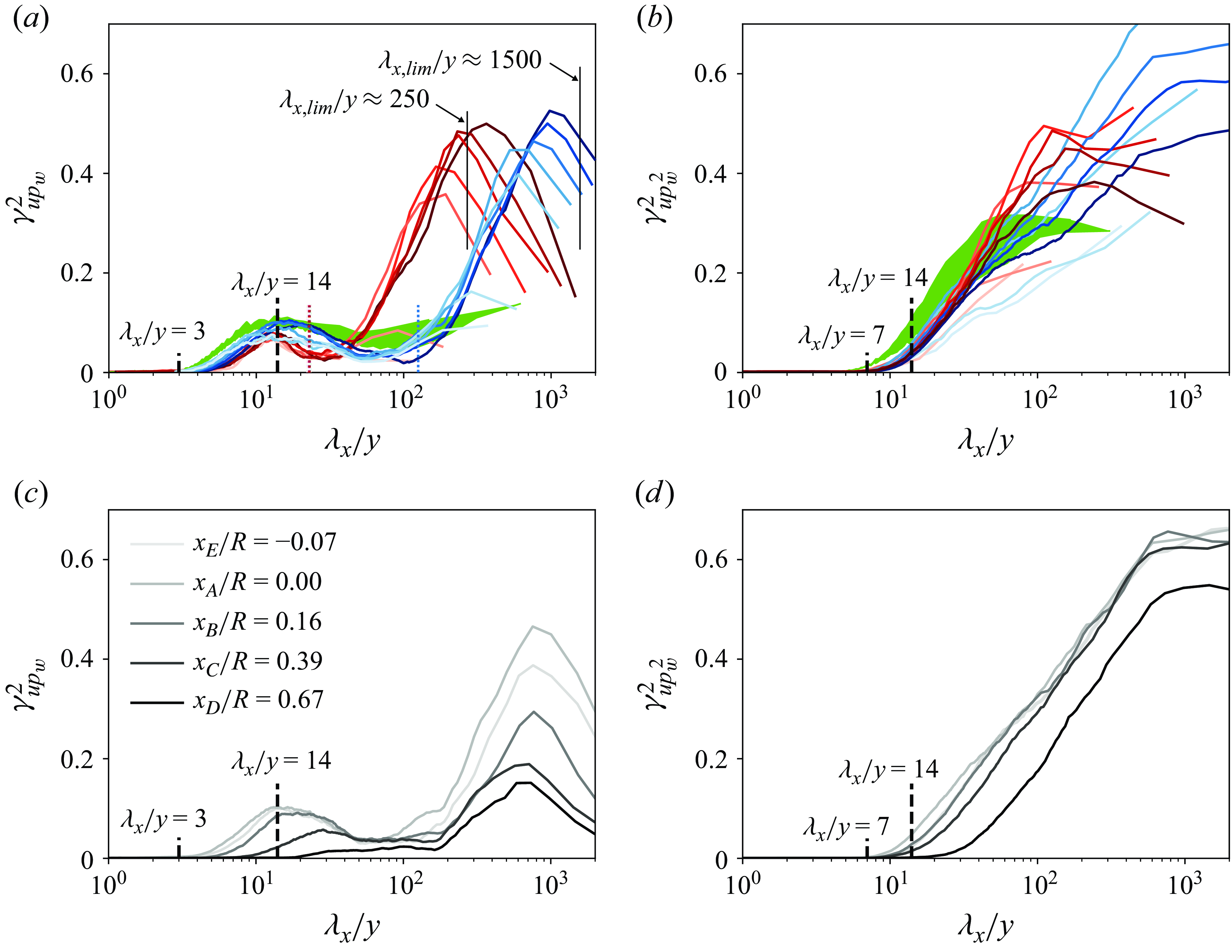
Figure 5. (a) Coherence spectra for the fluctuations in streamwise velocity and wall-pressure, and (b) the streamwise velocity and wall-pressure-squared. Two sets of coherence spectra are shown, corresponding to velocity fluctuations measured at point $A$
(blue colour scale) and point
$A$
(blue colour scale) and point $F$
(red colour scale); an increase in colour intensity corresponds to an increase in
$F$
(red colour scale); an increase in colour intensity corresponds to an increase in $Re_\tau$
following test cases
$Re_\tau$
following test cases $1\rightarrow 7$
, listed in table 1. Reference data are shown with a light grey shaded area, associated with the spread of coherence spectra from spatial DNS data at
$1\rightarrow 7$
, listed in table 1. Reference data are shown with a light grey shaded area, associated with the spread of coherence spectra from spatial DNS data at $Re_\tau = 5{}200$
(Baars et al. Reference Baars, Dacome and Lee2024). (c) Coherence spectra for the fluctuations in streamwise velocity and wall-pressure, and (d) the streamwise velocity and wall-pressure-squared, for test case 3 (
$Re_\tau = 5{}200$
(Baars et al. Reference Baars, Dacome and Lee2024). (c) Coherence spectra for the fluctuations in streamwise velocity and wall-pressure, and (d) the streamwise velocity and wall-pressure-squared, for test case 3 ( $Re_\tau \approx 14\,004$
), and for velocity fluctuations measured at points E, A–D spanning a range of streamwise locations,
$Re_\tau \approx 14\,004$
), and for velocity fluctuations measured at points E, A–D spanning a range of streamwise locations, $-0.07 \leqslant x/R \leqslant 0.67$
. Note that all current coherence spectra are generated from temporal data and plotted as spatial spectra by converting frequency into wavelength using
$-0.07 \leqslant x/R \leqslant 0.67$
. Note that all current coherence spectra are generated from temporal data and plotted as spatial spectra by converting frequency into wavelength using $\lambda _x \equiv U_c/f$
with
$\lambda _x \equiv U_c/f$
with $U_c^+ = 10$
. Data employed for plotting panels (a) and (b) are available in the supplementary material.
$U_c^+ = 10$
. Data employed for plotting panels (a) and (b) are available in the supplementary material.
Figures 5(a) and 5(b) present the LCS for $u$
and
$u$
and $p_w$
, for two positions of the velocity measurement (points
$p_w$
, for two positions of the velocity measurement (points $A$
and
$A$
and $F$
in figure 1
d) and for all values of
$F$
in figure 1
d) and for all values of $Re_\tau$
. In presenting the scale-dependent spectra, we resort to scaling
$Re_\tau$
. In presenting the scale-dependent spectra, we resort to scaling $\lambda _x$
with the distance-from-the-wall, so that the abscissae are in terms of
$\lambda _x$
with the distance-from-the-wall, so that the abscissae are in terms of $\lambda _x/y$
with
$\lambda _x/y$
with $y = \{y_{A},y_{F}\}$
for these graphs. With negligible coherence reported at small wavelengths, a steady rise in the LCS can be observed in figure 5(a) for increasing
$y = \{y_{A},y_{F}\}$
for these graphs. With negligible coherence reported at small wavelengths, a steady rise in the LCS can be observed in figure 5(a) for increasing $\lambda _x/y$
until a local maximum is reached at
$\lambda _x/y$
until a local maximum is reached at $(\lambda _x/y,\gamma _{up_w}^2) \approx (14,0.1)$
. Given that the current data span nearly a decade in
$(\lambda _x/y,\gamma _{up_w}^2) \approx (14,0.1)$
. Given that the current data span nearly a decade in $Re_\tau$
, we can conclude that the region of coherence centred at
$Re_\tau$
, we can conclude that the region of coherence centred at $\lambda _x/y \approx 14$
is Reynolds-number invariant. Only the two LCS corresponding to test cases 1 and 2 have a slightly lower value near
$\lambda _x/y \approx 14$
is Reynolds-number invariant. Only the two LCS corresponding to test cases 1 and 2 have a slightly lower value near $\lambda _x/y = 14$
. This is ascribed to the incomplete removal of facility noise in the wall-pressure spectra of these two test cases (recall the discussion in § 3), and the fact that additive noise in the spectra causes an attenuation of the LCS. Only a slight discrepancy in the
$\lambda _x/y = 14$
. This is ascribed to the incomplete removal of facility noise in the wall-pressure spectra of these two test cases (recall the discussion in § 3), and the fact that additive noise in the spectra causes an attenuation of the LCS. Only a slight discrepancy in the $\lambda _x/y$
locations of the local maxima in coherence appears between the sets of coherence spectra corresponding to point A (blue colour scale) and point B (red colour scale). The differences in the
$\lambda _x/y$
locations of the local maxima in coherence appears between the sets of coherence spectra corresponding to point A (blue colour scale) and point B (red colour scale). The differences in the $\lambda _x/y$
locations of the local maxima are marginal in comparison to the difference in wall-normal position (
$\lambda _x/y$
locations of the local maxima are marginal in comparison to the difference in wall-normal position ( $y_F \approx 6y_A$
). In fact, there is no evidence that the locations of the maxima depend on the wall-normal location being considered, as the coherence spectra from DNS data – corresponding to various wall-normal locations being considered – show excellent collapse when
$y_F \approx 6y_A$
). In fact, there is no evidence that the locations of the maxima depend on the wall-normal location being considered, as the coherence spectra from DNS data – corresponding to various wall-normal locations being considered – show excellent collapse when $\lambda _x$
is scaled with the distance-from-the-wall (Baars et al. Reference Baars, Dacome and Lee2024).
$\lambda _x$
is scaled with the distance-from-the-wall (Baars et al. Reference Baars, Dacome and Lee2024).
A second region of significant coherence appears at large wavelengths. This region manifests itself by a Reynolds-number-invariant rise in coherence (from approximately the wavelengths indicated with the vertical dotted lines in figure 5
a), up to wavelengths where the velocity fluctuations continue to be energetically relevant. To illustrate this, an amplitude threshold of the pre-multiplied streamwise energy spectra is taken as $k^+_x\phi ^+_{uu} = 0.2$
at the large-scale end. Energy levels only drop below this threshold for outer-scaled wavelengths of
$k^+_x\phi ^+_{uu} = 0.2$
at the large-scale end. Energy levels only drop below this threshold for outer-scaled wavelengths of $\lambda _{x,{lim}}/R \gtrsim 35$
. This limit is included in figure 5(a) for reference and corresponds to
$\lambda _{x,{lim}}/R \gtrsim 35$
. This limit is included in figure 5(a) for reference and corresponds to $\lambda _{x,{lim}}/y \approx \{250,1{}500\}$
for
$\lambda _{x,{lim}}/y \approx \{250,1{}500\}$
for $y = \{y_A,y_F\}$
, respectively.
$y = \{y_A,y_F\}$
, respectively.
This large-scale region of strong coherence between $u$
fluctuations in the logarithmic region and the wall-pressure field is presumably related to global velocity modes (Bullock, Cooper & Abernathy Reference Bullock, Cooper and Abernathy1978; del Á lamo &Jiménez Reference del Álamo and Jiménez2003). These global modes are ‘inactive’ in the view of Townsend’s attached-eddy hypothesis (Townsend Reference Townsend1976) (thus, large-scale eddies that do not contribute to the Reynolds shear stress
$u$
fluctuations in the logarithmic region and the wall-pressure field is presumably related to global velocity modes (Bullock, Cooper & Abernathy Reference Bullock, Cooper and Abernathy1978; del Á lamo &Jiménez Reference del Álamo and Jiménez2003). These global modes are ‘inactive’ in the view of Townsend’s attached-eddy hypothesis (Townsend Reference Townsend1976) (thus, large-scale eddies that do not contribute to the Reynolds shear stress $uv$
). Inactive motions are coupled to the very large scales in the pressure spectrum (
$uv$
). Inactive motions are coupled to the very large scales in the pressure spectrum ( $TU_\infty /\delta \gt 7$
, with
$TU_\infty /\delta \gt 7$
, with $T$
being their characteristic period and
$T$
being their characteristic period and $\delta$
the boundary layer thickness) (as shown explicitly by Deshpande et al. Reference Deshpande, Vinuesa, Klewicki and Marusic2025), while the active motions contribute directly to the intermediate scales (
$\delta$
the boundary layer thickness) (as shown explicitly by Deshpande et al. Reference Deshpande, Vinuesa, Klewicki and Marusic2025), while the active motions contribute directly to the intermediate scales ( $0.8\lt TU_\infty /\delta \lt 7$
). The limit of
$0.8\lt TU_\infty /\delta \lt 7$
). The limit of $TU_\infty /R=7$
is identified in figure 5(a), for the measurements corresponding to point
$TU_\infty /R=7$
is identified in figure 5(a), for the measurements corresponding to point $y_A$
and point
$y_A$
and point $y_F$
, by means of the blue and red vertical dotted lines at the corresponding
$y_F$
, by means of the blue and red vertical dotted lines at the corresponding $\lambda _x/y$
values, respectively.
$\lambda _x/y$
values, respectively.
Before further discussing the trends of the coherence spectra, we proceed with inspecting the coherence involving the quadratic term of the wall-pressure. The inclusion of this term was deemed important for stochastically estimating off-the-wall velocities from wall-pressure data. The quadratic term of the wall-pressure is taken as $p_w^2 = [p_w^2]_{r} - \overline { [p_w^2]_{r}}$
, with
$p_w^2 = [p_w^2]_{r} - \overline { [p_w^2]_{r}}$
, with $ [p_w^2]_{r}$
denoting the time series of the wall-pressure-squared prior to the subtraction of its mean. Different to the behaviour displayed by the linear term of wall-pressure, the LCS for
$ [p_w^2]_{r}$
denoting the time series of the wall-pressure-squared prior to the subtraction of its mean. Different to the behaviour displayed by the linear term of wall-pressure, the LCS for $u$
and
$u$
and $p_w^2$
rises starting from
$p_w^2$
rises starting from $\lambda _x/y \approx 7$
(see figure 5
b). Again, a Reynolds-number-invariant trend appears in the rise of coherence around scales of
$\lambda _x/y \approx 7$
(see figure 5
b). Again, a Reynolds-number-invariant trend appears in the rise of coherence around scales of $\lambda _x/y = 14$
and beyond, with once more the LCS of test cases 1 and 2 comprising a lower magnitude due to the incomplete removal of facility noise from the wall-pressure spectra. To further conclude the Reynolds-number-invariant trends observed in figure 5(a,b), the current experimental coherence spectra generated from temporal data are compared with the coherence spectra presented by Baars et al. (Reference Baars, Dacome and Lee2024), generated from spatial DNS data of turbulent channel flow. These reference data are shown with the light grey shaded area, indicating the spread of coherence spectra at
$\lambda _x/y = 14$
and beyond, with once more the LCS of test cases 1 and 2 comprising a lower magnitude due to the incomplete removal of facility noise from the wall-pressure spectra. To further conclude the Reynolds-number-invariant trends observed in figure 5(a,b), the current experimental coherence spectra generated from temporal data are compared with the coherence spectra presented by Baars et al. (Reference Baars, Dacome and Lee2024), generated from spatial DNS data of turbulent channel flow. These reference data are shown with the light grey shaded area, indicating the spread of coherence spectra at $Re_\tau = 5{}200$
when considering a range of wall-normal positions across the logarithmic region (
$Re_\tau = 5{}200$
when considering a range of wall-normal positions across the logarithmic region ( $80 \lesssim y^+ \lesssim 0.15Re_\tau$
, see figure 6 of Baars et al. Reference Baars, Dacome and Lee2024). Moreover, Baars et al. (Reference Baars, Dacome and Lee2024) also revealed a Reynolds-number-invariant trend for these DNS data, spanning
$80 \lesssim y^+ \lesssim 0.15Re_\tau$
, see figure 6 of Baars et al. Reference Baars, Dacome and Lee2024). Moreover, Baars et al. (Reference Baars, Dacome and Lee2024) also revealed a Reynolds-number-invariant trend for these DNS data, spanning $550\lesssim Re_\tau \lesssim \approx 5200$
. It must be noted that even though these DNS data are associated with turbulent channel flow, it was shown that coherence spectra from a relatively low-Reynolds-number TBL flow (
$550\lesssim Re_\tau \lesssim \approx 5200$
. It must be noted that even though these DNS data are associated with turbulent channel flow, it was shown that coherence spectra from a relatively low-Reynolds-number TBL flow ( $Re_\tau \approx 2280$
) were also in agreement with these channel flow data. Therefore, with the current LCS for pipe flow collapsing for the full range of
$Re_\tau \approx 2280$
) were also in agreement with these channel flow data. Therefore, with the current LCS for pipe flow collapsing for the full range of $Re_\tau$
, for both wall-normal positions,
$Re_\tau$
, for both wall-normal positions, $y = \{y_{A},y_{F}\}$
(while agreeing with the reference data), it can be concluded that the coherence is statistically similar across several canonical flow geometries.
$y = \{y_{A},y_{F}\}$
(while agreeing with the reference data), it can be concluded that the coherence is statistically similar across several canonical flow geometries.
Universal trends in the coherence spectra are reflective of how coherent velocity fluctuations are interlinked to the wall-pressure. The scales around which $\gamma ^2_{up_w}$
and
$\gamma ^2_{up_w}$
and $\gamma ^2_{up^2_w}$
become non-zero (
$\gamma ^2_{up^2_w}$
become non-zero ( $\lambda _x/y \approx 3$
and
$\lambda _x/y \approx 3$
and $\lambda _x/y \approx 7$
, respectively), as well as the logarithmic growth of coherence (most noticeable in figure 5(b), where
$\lambda _x/y \approx 7$
, respectively), as well as the logarithmic growth of coherence (most noticeable in figure 5(b), where $\gamma ^2_{up^2_w} \propto \ln (\lambda _x/y)$
) follow a pattern presented in the work by Baars et al. (Reference Baars, Hutchins and Marusic2017). They considered the coherence between the near-wall velocity fluctuations and those in the logarithmic region. The logarithmic growth of coherence, which occurs over the inertial range of wavelengths, was interpreted as the range of scales that contains turbulence energy that is statistically self-similar (following a hierarchical structure of wall-attached eddies).
$\gamma ^2_{up^2_w} \propto \ln (\lambda _x/y)$
) follow a pattern presented in the work by Baars et al. (Reference Baars, Hutchins and Marusic2017). They considered the coherence between the near-wall velocity fluctuations and those in the logarithmic region. The logarithmic growth of coherence, which occurs over the inertial range of wavelengths, was interpreted as the range of scales that contains turbulence energy that is statistically self-similar (following a hierarchical structure of wall-attached eddies).

Figure 6. (a) Normalised wall-pressure time series of microphone $\mathcal{M}1$
, for test case 3 (
$\mathcal{M}1$
, for test case 3 ( $Re_\tau \approx 14\,004$
), its Hilbert transform and the corresponding de-meaned wall-pressure-squared. (b) Coherence spectra for the fluctuations in streamwise velocity and wall-pressure-squared (dashed lines, identical to the coherence spectra in figure 5
b), compared with the coherence spectra for fluctuations in the streamwise velocity at point
$Re_\tau \approx 14\,004$
), its Hilbert transform and the corresponding de-meaned wall-pressure-squared. (b) Coherence spectra for the fluctuations in streamwise velocity and wall-pressure-squared (dashed lines, identical to the coherence spectra in figure 5
b), compared with the coherence spectra for fluctuations in the streamwise velocity at point $y_A$
and the Hilbert transform of the wall-pressure (solid lines).
$y_A$
and the Hilbert transform of the wall-pressure (solid lines).
An increase in large-scale coherence for the wall-pressure-squared term suggests that large-scale $u$
fluctuations modify (modulate) the wall-pressure field following nonlinear dynamics. To analyse this phenomenon, a Hilbert transform is used to retrieve an ‘envelope’ of the wall-pressure time series. Figure 6(a) presents the normalised wall-pressure time series (
$u$
fluctuations modify (modulate) the wall-pressure field following nonlinear dynamics. To analyse this phenomenon, a Hilbert transform is used to retrieve an ‘envelope’ of the wall-pressure time series. Figure 6(a) presents the normalised wall-pressure time series ( $\widetilde {p}_w = p_w/p^{\prime }_w$
) at
$\widetilde {p}_w = p_w/p^{\prime }_w$
) at $Re_\tau \approx 14\,004$
for microphone
$Re_\tau \approx 14\,004$
for microphone $\mathcal{M}1$
, over a short time interval, together with the magnitude of its Hilbert transform,
$\mathcal{M}1$
, over a short time interval, together with the magnitude of its Hilbert transform, $\vert H(\widetilde {p}_w) \vert$
, and the de-meaned wall-pressure-squared time series. By visual inspection, these last two time series have similar large-scale energy content. Figure 6(b) quantifies this further by overlaying the LCS for
$\vert H(\widetilde {p}_w) \vert$
, and the de-meaned wall-pressure-squared time series. By visual inspection, these last two time series have similar large-scale energy content. Figure 6(b) quantifies this further by overlaying the LCS for $u$
and
$u$
and $\vert H(\widetilde {p}_w)\vert$
, and the LCS for
$\vert H(\widetilde {p}_w)\vert$
, and the LCS for $u$
and
$u$
and $p_w^2$
. A remarkable collapse is observed for the two sets of LCS spectra, for all
$p_w^2$
. A remarkable collapse is observed for the two sets of LCS spectra, for all $Re_\tau$
cases considered. Hence, the large-scale variations in the wall-pressure intensity are directly linked to the passage of streamwise velocity fluctuations modulating the near-wall intensity (Tsuji et al. Reference Tsuji, Marusic and Johansson2015).
$Re_\tau$
cases considered. Hence, the large-scale variations in the wall-pressure intensity are directly linked to the passage of streamwise velocity fluctuations modulating the near-wall intensity (Tsuji et al. Reference Tsuji, Marusic and Johansson2015).
Gaining knowledge on how the coherence decays as a function of the streamwise separation between the velocity measurement and the wall-pressure sensor is highly relevant for real-time flow control (e.g. when sensors and actuators are separated to allow for control actions while the flow convects downstream). For our current data, the $\gamma ^2_{up_w}$
and
$\gamma ^2_{up_w}$
and $\gamma ^2_{up^2_w}$
coherence spectra are considered as a function of the streamwise distance of the velocity measurement (relative to the wall-pressure sensor at
$\gamma ^2_{up^2_w}$
coherence spectra are considered as a function of the streamwise distance of the velocity measurement (relative to the wall-pressure sensor at $x = 0$
) for test case 3 corresponding to
$x = 0$
) for test case 3 corresponding to $Re_\tau \approx 14\,004$
. Coherence spectra are shown in figures 5(c) and 5(d), for
$Re_\tau \approx 14\,004$
. Coherence spectra are shown in figures 5(c) and 5(d), for $\gamma ^2_{up_w}$
and
$\gamma ^2_{up_w}$
and $\gamma ^2_{up^2_w}$
, respectively. When increasing the streamwise distance,
$\gamma ^2_{up^2_w}$
, respectively. When increasing the streamwise distance, $\gamma ^2_{up_w}$
decays with the coherence decreasing faster at smaller scales, as is expected. Similar conclusions were drawn for all other
$\gamma ^2_{up_w}$
decays with the coherence decreasing faster at smaller scales, as is expected. Similar conclusions were drawn for all other $Re_\tau$
test cases. When inspecting the decay in
$Re_\tau$
test cases. When inspecting the decay in $\gamma _{up_w^2}^2$
(figure 5
d), it becomes clear that the coherence with the quadratic wall-pressure term remains considerably larger than with the linear term. This means that the mechanism of large-scale modulation of the smaller-scale wall-pressure fluctuations (by the large-scale
$\gamma _{up_w^2}^2$
(figure 5
d), it becomes clear that the coherence with the quadratic wall-pressure term remains considerably larger than with the linear term. This means that the mechanism of large-scale modulation of the smaller-scale wall-pressure fluctuations (by the large-scale $u$
fluctuations) is dominant over the direct (linear) imprint of
$u$
fluctuations) is dominant over the direct (linear) imprint of $u$
fluctuations on the wall-pressure.
$u$
fluctuations on the wall-pressure.
5. Coherence between wall-normal velocity and wall-pressure fluctuations
To further characterise the dynamics between fluctuations in velocity and wall-pressure, the foregoing presents a similar analysis as described in § 4, but instead of considering the $u$
fluctuations, we concentrate on the
$u$
fluctuations, we concentrate on the $v$
fluctuations. Coherence spectra for
$v$
fluctuations. Coherence spectra for $v$
and
$v$
and $p_w$
(figure 7
a) exhibit local maxima around
$p_w$
(figure 7
a) exhibit local maxima around $\lambda _x/y \approx 10$
(instead of
$\lambda _x/y \approx 10$
(instead of $\lambda _x/y \approx 8$
, as indicated by Baars et al. Reference Baars, Dacome and Lee2024) and
$\lambda _x/y \approx 8$
, as indicated by Baars et al. Reference Baars, Dacome and Lee2024) and $\gamma _{vp_w}^2\approx 0.15$
, a magnitude which is roughly 50 % higher than local maxima in the LCS for
$\gamma _{vp_w}^2\approx 0.15$
, a magnitude which is roughly 50 % higher than local maxima in the LCS for $u$
and
$u$
and $p_w$
. Squaring the wall-pressure fluctuations brings higher levels of
$p_w$
. Squaring the wall-pressure fluctuations brings higher levels of $\gamma _{vp_w^2}^2$
(see figure 7
b), starting to rise at
$\gamma _{vp_w^2}^2$
(see figure 7
b), starting to rise at $\lambda _x/y \approx 3$
. A similar Reynolds-number independence is observed as was seen in the coherence analyses with the
$\lambda _x/y \approx 3$
. A similar Reynolds-number independence is observed as was seen in the coherence analyses with the $u$
fluctuations.
$u$
fluctuations.
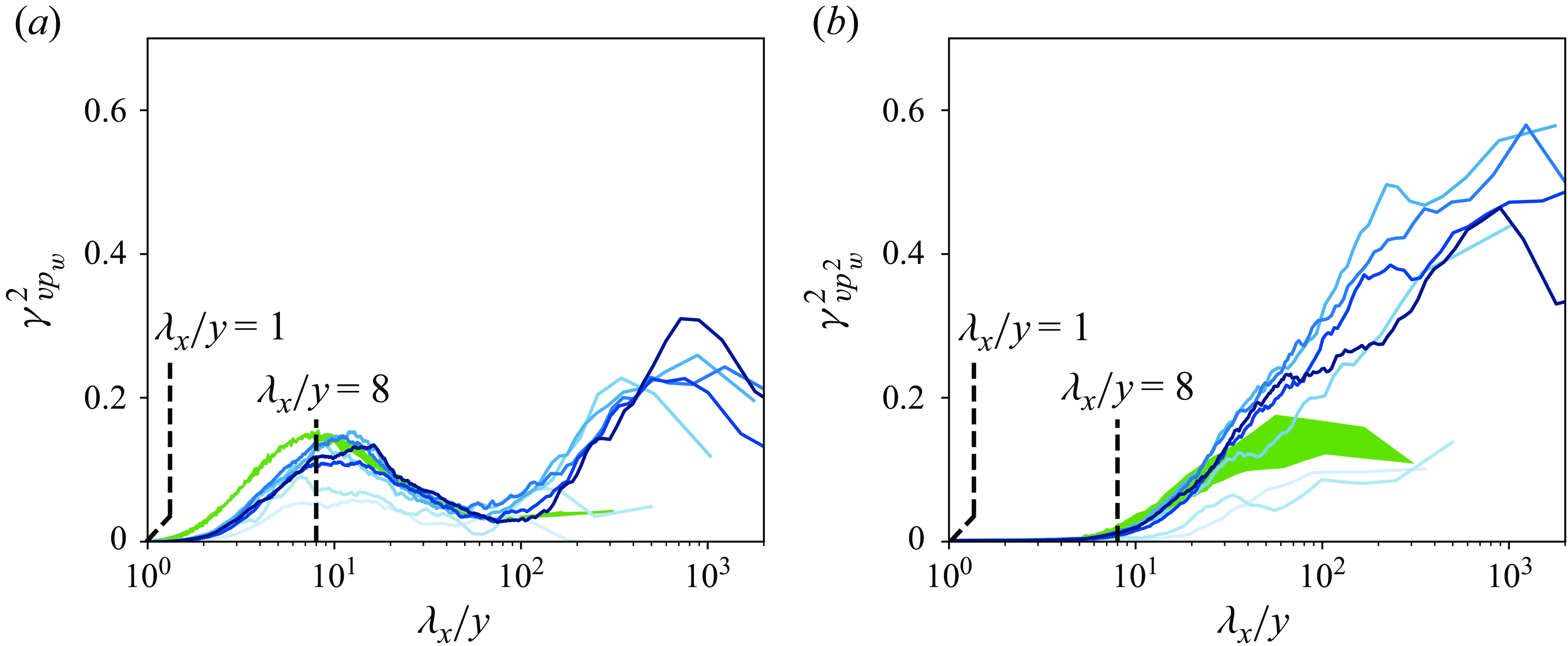
Figure 7. (a) Coherence spectra for the fluctuations in wall-normal velocity and wall-pressure, and (b) the wall-normal velocity and wall-pressure-squared. Two sets of coherence spectra are shown, corresponding to velocity fluctuations measured at point $A$
; an increase in colour intensity corresponds to an increase in
$A$
; an increase in colour intensity corresponds to an increase in $Re_\tau$
following test cases
$Re_\tau$
following test cases $1\rightarrow 7$
, listed in table 1. The light grey shaded area is associated with the spread of coherence spectra from DNS data, as reported by Baars et al. (Reference Baars, Dacome and Lee2024). Note that all current coherence spectra are generated from temporal data and plotted as spatial spectra by converting frequency into wavelength using
$1\rightarrow 7$
, listed in table 1. The light grey shaded area is associated with the spread of coherence spectra from DNS data, as reported by Baars et al. (Reference Baars, Dacome and Lee2024). Note that all current coherence spectra are generated from temporal data and plotted as spatial spectra by converting frequency into wavelength using $\lambda _x \equiv U_c/f$
with
$\lambda _x \equiv U_c/f$
with $U_c^+ = 10$
. Data employed for plotting panels (a) and (b) are available in the supplementary material.
$U_c^+ = 10$
. Data employed for plotting panels (a) and (b) are available in the supplementary material.
Higher coherence between wall-normal velocity and wall-pressure fluctuations complies with earlier findings (e.g. Gibeau & Ghaemi Reference Gibeau and Ghaemi2021). In fact, given the non-permeability boundary condition, fluid motions directed towards the wall (with a negative $v$
-component) will stagnate and thus give rise to a positive fluctuation in wall-pressure. Conversely,
$v$
-component) will stagnate and thus give rise to a positive fluctuation in wall-pressure. Conversely, $v \gt 0$
fluctuations will tend to lower the unsteady wall-pressure. In general, the higher correlation between
$v \gt 0$
fluctuations will tend to lower the unsteady wall-pressure. In general, the higher correlation between $v$
and
$v$
and $p_w$
can be ascribed to the Orr mechanism (see Jiménez Reference Jiménez2013; Luhar et al. Reference Luhar, Sharma and McKeon2014, among others). Therefore, there exists a rather strong coupling between
$p_w$
can be ascribed to the Orr mechanism (see Jiménez Reference Jiménez2013; Luhar et al. Reference Luhar, Sharma and McKeon2014, among others). Therefore, there exists a rather strong coupling between $v$
and
$v$
and $p_w$
. Note, however, that our current work is motivated by using wall-pressure information to, eventually, predict the off-the-wall velocity fluctuations. Using pressure information to predict wall-normal velocity fluctuations for real-time control is not as effective as when considering streamwise velocity fluctuations, because the streamwise ones provide a stronger contribution to wall-shear stress generating mechanisms (e.g. Deck et al. Reference Deck, Renhard, Laraufie and Weiss2014, among others). Furthermore,
$p_w$
. Note, however, that our current work is motivated by using wall-pressure information to, eventually, predict the off-the-wall velocity fluctuations. Using pressure information to predict wall-normal velocity fluctuations for real-time control is not as effective as when considering streamwise velocity fluctuations, because the streamwise ones provide a stronger contribution to wall-shear stress generating mechanisms (e.g. Deck et al. Reference Deck, Renhard, Laraufie and Weiss2014, among others). Furthermore, $v$
fluctuations have a considerably shorter characteristic wavelength than
$v$
fluctuations have a considerably shorter characteristic wavelength than $u$
fluctuations (
$u$
fluctuations ( $\lambda _x^+ \approx 250$
for the former and
$\lambda _x^+ \approx 250$
for the former and $\lambda _x^+ \approx 1000$
for the latter). This not only requires faster processing for real-time operations, but would also constrain the sensor-actuator spacing due to the faster de-correlation of the
$\lambda _x^+ \approx 1000$
for the latter). This not only requires faster processing for real-time operations, but would also constrain the sensor-actuator spacing due to the faster de-correlation of the $v$
fluctuations in the streamwise direction.
$v$
fluctuations in the streamwise direction.
6. Stochastic estimation of streamwise velocity fluctuations
For real-time control purposes, wall-pressure sensing can be employed to generate an estimate of the fluctuating velocities in the logarithmic region of a wall-bounded turbulent flow. To this end, the foregoing will examine the accuracy of the prediction of $u$
fluctuations, performed with Linear and Quadratic Stochastic Estimation methods (LSE and QSE, respectively). These methods solely employ the time series of wall-pressure and wall-pressure-squared, as the input quantities.
$u$
fluctuations, performed with Linear and Quadratic Stochastic Estimation methods (LSE and QSE, respectively). These methods solely employ the time series of wall-pressure and wall-pressure-squared, as the input quantities.
Estimates of the $u$
fluctuations in the logarithmic region at position
$u$
fluctuations in the logarithmic region at position $y_e$
can be formed through a convolution of time-domain kernels. Estimates of unconditional time series of off-the-wall velocity fluctuations, with the LSE and QSE procedures, follow from the formulations:
$y_e$
can be formed through a convolution of time-domain kernels. Estimates of unconditional time series of off-the-wall velocity fluctuations, with the LSE and QSE procedures, follow from the formulations:
 \begin{eqnarray} \widehat {u}_{\textit{LSE}}\left (y_e,t\right) &=& \left (h_l \circledast p_w \right)\left (t\right), \\[-27pt] \nonumber \end{eqnarray}
 \begin{eqnarray} \widehat {u}_{\textit{QSE}}\left (y_e,t\right) &=& \left (h_l \circledast p_w \right)\left (t\right) + \left (h_q \circledast p^2_w \right)\left (t\right), \end{eqnarray}
where the (stochastic) temporal kernels of the linear term ( $h_l$
) and quadratic term (
$h_l$
) and quadratic term ( $h_q$
) are the inverse Fourier transforms of the complex, frequency-domain kernels, e.g.
$h_q$
) are the inverse Fourier transforms of the complex, frequency-domain kernels, e.g. $h_l (y_e,t) = \mathcal{F}^{-1} [H_L (y_e,f)]$
and similar for
$h_l (y_e,t) = \mathcal{F}^{-1} [H_L (y_e,f)]$
and similar for $h_q$
. The linear kernel equals the cross-spectrum between
$h_q$
. The linear kernel equals the cross-spectrum between $u$
and
$u$
and $p_w$
, divided by the auto-spectra of
$p_w$
, divided by the auto-spectra of $p_w$
(the input quantity during the estimation method),
$p_w$
(the input quantity during the estimation method),
 \begin{equation} H_L\left (y_e,f\right) = \frac {\langle \widetilde {U}\left (y_e,f\right) \widetilde {P}^*_w\left (f\right) \rangle }{\langle \vert \widetilde {P}_w\left (f\right) \vert ^2 \rangle }, \end{equation}
whereas the quadratic kernel includes the wall-pressure-squared term, $p_w^2$
, instead of the linear one,
$p_w^2$
, instead of the linear one,
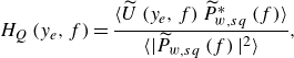 \begin{equation} H_Q\left (y_e,f\right) = \frac {\langle \widetilde {U}\left (y_e,f\right) \widetilde {P}^*_{w,sq}\left (f\right) \rangle }{\langle \vert \widetilde {P}_{w,sq}\left (f\right) \vert ^2 \rangle }, \end{equation}
with $\widetilde {P}_{w,sq} (f) = \mathcal{F} [p^2_w(t)]$
. Given our current dataset, two estimation locations are considered (
$\widetilde {P}_{w,sq} (f) = \mathcal{F} [p^2_w(t)]$
. Given our current dataset, two estimation locations are considered ( $y_e = y_A$
and
$y_e = y_A$
and $y_e = y_F$
). Further details of the stochastic estimation procedures can be found elsewhere (Naguib et al. Reference Naguib, Wark and Juckenhöfel2001; Baars et al. Reference Baars, Dacome and Lee2024).
$y_e = y_F$
). Further details of the stochastic estimation procedures can be found elsewhere (Naguib et al. Reference Naguib, Wark and Juckenhöfel2001; Baars et al. Reference Baars, Dacome and Lee2024).
To evaluate the accuracy of the estimation with respect to the reference time series, $u(y_0,t)$
, the Pearson correlation coefficient is employed. It is defined as the ratio of the covariance of two input signals to the product of the standard deviation of the two. Figure 8(b) presents values of
$u(y_0,t)$
, the Pearson correlation coefficient is employed. It is defined as the ratio of the covariance of two input signals to the product of the standard deviation of the two. Figure 8(b) presents values of $\rho [u_W(y,t),\widehat {u}_{{ QSE}}(y,t)]= \mathrm{cov} [u_W(y,t),\widehat {u}_{{ QSE}}(y,t)]/(u_W^{\prime} \widehat{u}^{\kern1pt \prime}_{{ QSE}})$
: the correlation coefficient between the reference time series
$\rho [u_W(y,t),\widehat {u}_{{ QSE}}(y,t)]= \mathrm{cov} [u_W(y,t),\widehat {u}_{{ QSE}}(y,t)]/(u_W^{\prime} \widehat{u}^{\kern1pt \prime}_{{ QSE}})$
: the correlation coefficient between the reference time series $u_W(y,t)$
at points
$u_W(y,t)$
at points $A$
and
$A$
and $F$
(see figure 1
b) to the QSE-based time series,
$F$
(see figure 1
b) to the QSE-based time series, $\widehat {u}_{{ QSE}}(y,t)$
. Here, the time series
$\widehat {u}_{{ QSE}}(y,t)$
. Here, the time series $u_W(y,t)$
is not equal to
$u_W(y,t)$
is not equal to $u(y,t)$
, because
$u(y,t)$
, because $u_W$
only retains wall-attached eddies. Effectively,
$u_W$
only retains wall-attached eddies. Effectively, $u_W$
is a large-scale pass-filtered signal of
$u_W$
is a large-scale pass-filtered signal of $u$
, with its Reynolds number-invariant kernel characterised by a definitive cutoff at
$u$
, with its Reynolds number-invariant kernel characterised by a definitive cutoff at $\lambda _x/y = 14$
(Baars et al. Reference Baars, Hutchins and Marusic2017).
$\lambda _x/y = 14$
(Baars et al. Reference Baars, Hutchins and Marusic2017).
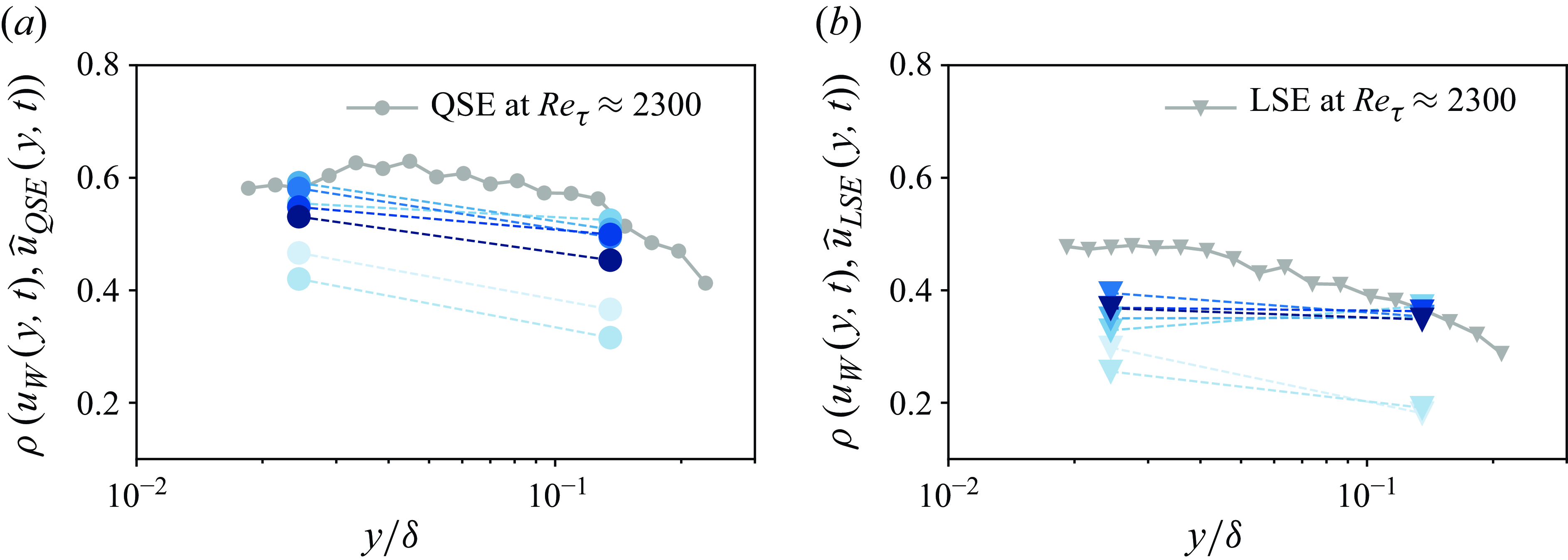
Figure 8. (a) Correlation coefficient computed with the QSE-based streamwise velocity fluctuations in the logarithmic region, $\widehat {u}_{{ QSE}}$
, and the reference time series,
$\widehat {u}_{{ QSE}}$
, and the reference time series, $u_W$
. (b) Correlation coefficient computed with the LSE-based streamwise velocity fluctuations in the logarithmic region,
$u_W$
. (b) Correlation coefficient computed with the LSE-based streamwise velocity fluctuations in the logarithmic region, $\widehat {u}_{{ LSE}}$
, and the reference time series,
$\widehat {u}_{{ LSE}}$
, and the reference time series, $u_W$
. Reference data are taken from Baars et al. (Reference Baars, Dacome and Lee2024) at
$u_W$
. Reference data are taken from Baars et al. (Reference Baars, Dacome and Lee2024) at $Re_\tau \approx 2300$
.
$Re_\tau \approx 2300$
.
With the exception of the data at the two lowest $Re_\tau$
test cases 1 and 2 – whose time series are still affected by imperfect noise filtering (see § 2.4) – we observe collapse for all
$Re_\tau$
test cases 1 and 2 – whose time series are still affected by imperfect noise filtering (see § 2.4) – we observe collapse for all $Re_\tau$
test cases considered. A slight attenuation of
$Re_\tau$
test cases considered. A slight attenuation of $\rho$
is observed with respect to the reference data, which is attributed to a systematic error (Saccenti et al. Reference Saccenti, Hendriks and Smilde2020) caused by additive facility noise. Furthermore, the data are in good agreement with the reference data from Baars et al. (Reference Baars, Dacome and Lee2024) at
$\rho$
is observed with respect to the reference data, which is attributed to a systematic error (Saccenti et al. Reference Saccenti, Hendriks and Smilde2020) caused by additive facility noise. Furthermore, the data are in good agreement with the reference data from Baars et al. (Reference Baars, Dacome and Lee2024) at $Re_\tau \approx 2300$
. This result solidifies the conclusion of Reynolds-number-independent estimation accuracy of wall-attached velocity fluctuations, based on wall-pressure sensing alone. As expected, a lower correlation coefficient appears in figure 8(b), where the estimation is performed with only the linear term of wall-pressure (thus, using the LSE method). The performance of the statistical estimator now decays by approximately 20 % with respect to QSE-based estimation, across the given range of wall-normal distances.
$Re_\tau \approx 2300$
. This result solidifies the conclusion of Reynolds-number-independent estimation accuracy of wall-attached velocity fluctuations, based on wall-pressure sensing alone. As expected, a lower correlation coefficient appears in figure 8(b), where the estimation is performed with only the linear term of wall-pressure (thus, using the LSE method). The performance of the statistical estimator now decays by approximately 20 % with respect to QSE-based estimation, across the given range of wall-normal distances.
7. Conclusions
Statistical correlations of hydrodynamic wall-pressure and velocity fluctuations in the logarithmic region of a turbulent pipe flow were experimentally investigated. With a unique dataset acquired in the CICLoPE long-pipe facility, spanning a large range of friction Reynolds numbers ( $4{}794 \lesssim Re_\tau \lesssim 47\,015$
), this study reveals definitive Reynolds number trends of the scale-dependent wall-pressure–velocity coherence. For the linear coherence between the
$4{}794 \lesssim Re_\tau \lesssim 47\,015$
), this study reveals definitive Reynolds number trends of the scale-dependent wall-pressure–velocity coherence. For the linear coherence between the $u$
velocity (and
$u$
velocity (and $v$
velocity) and wall-pressure, a Reynolds-number-independent scaling of the coherence spectra appears at the intermediate scale range when scaled with distance-from-the-wall. This trend is also statistically similar across several wall-bounded flows when compared with the data available from the open literature. When the squared wall-pressure fluctuations are considered instead of the linear wall-pressure, the coherence spectra for the wall-pressure and velocity fluctuations are higher in amplitude at the (very) large-scale end of the spectra. Physically, this link between wall-pressure-squared and velocity typifies a modulation effect as squaring the wall-pressure introduces low-frequency content that is reflective of how the higher-frequency wall-pressure intensity varies. Current findings of the coherence spectra bear relevance to stochastic estimation schemes, in which wall-pressure can be considered as an input to estimate off-the-wall velocity fluctuations. With the aid of a quadratic stochastic estimation method, it was shown that for each
$v$
velocity) and wall-pressure, a Reynolds-number-independent scaling of the coherence spectra appears at the intermediate scale range when scaled with distance-from-the-wall. This trend is also statistically similar across several wall-bounded flows when compared with the data available from the open literature. When the squared wall-pressure fluctuations are considered instead of the linear wall-pressure, the coherence spectra for the wall-pressure and velocity fluctuations are higher in amplitude at the (very) large-scale end of the spectra. Physically, this link between wall-pressure-squared and velocity typifies a modulation effect as squaring the wall-pressure introduces low-frequency content that is reflective of how the higher-frequency wall-pressure intensity varies. Current findings of the coherence spectra bear relevance to stochastic estimation schemes, in which wall-pressure can be considered as an input to estimate off-the-wall velocity fluctuations. With the aid of a quadratic stochastic estimation method, it was shown that for each $Re_\tau$
investigated, the estimated time series and a true temporal measurement of velocity inside the turbulent pipe flow yielded a normalised correlation coefficient of up to
$Re_\tau$
investigated, the estimated time series and a true temporal measurement of velocity inside the turbulent pipe flow yielded a normalised correlation coefficient of up to $\rho \approx 0.6$
(while this was below 0.4 for a linear stochastic estimation method excluding the wall-pressure-squared term). This demonstrates that (sparse) wall-pressure sensing can be employed for meaningful estimation of off-the-wall velocity fluctuations. Additionally, wall-pressure as an input for estimation schemes is scalable to application-level conditions.
$\rho \approx 0.6$
(while this was below 0.4 for a linear stochastic estimation method excluding the wall-pressure-squared term). This demonstrates that (sparse) wall-pressure sensing can be employed for meaningful estimation of off-the-wall velocity fluctuations. Additionally, wall-pressure as an input for estimation schemes is scalable to application-level conditions.
Supplementary materials
Supplementary materials are available at https://doi.org/10.1017/jfm.2025.400.
Acknowledgements
We thank the Dipartimento di Ingegneria Industriale (DIN Department) of the University of Bologna for granting a Young Visiting Fellowship, enabling an on-site visit for G.D. and W.J.B. We also acknowledge the technical staff in Forlì for the support during the experiments.
Funding
The work of the UniBo team was carried out within the MOST – Sustainable Mobility National Research Center – and received funding from the European Union Next-GenerationEU [PIANO NAZIONALE DI RIPRESA E RESILIENZA (PNRR) – MISSIONE 4 COMPONENTE 2, INVESTIMENTO 1.4 – D.D. 1033 17/06/2022, CN00000023].
Declaration of interests
The authors report no conflict of interest.
Appendix A. Removing facility noise from the experimental wall-pressure signals
Wall-pressure measurements by means of microphones, mounted within sub-surface cavities communicating with the flow through a pinhole orifice, result in signal contamination from two main sources: (1) acoustic noise from the flow facility and (2) acoustic resonance as a consequence of the pinhole–sub-surface-cavity geometry. While a correction for the latter can directly be implemented in the frequency domain and takes the form of a division of the spectrum by the gain-squared of a correction kernel (as done in § 3), the former requires a more elaborate procedure. In particular, when considering a raw pressure time series of one of the microphones in figure 1(c), it is necessary to disambiguate hydrodynamic wall-pressure signatures from those induced by acoustic phenomena. In the case of turbulence-induced fluctuations, especially wall-pressure, they possess negligible streamwise and spanwise (azimuthal) coherence when considering relatively large sensor separations. Acoustic pressure fluctuations, however, convect from sensor to sensor retaining high correlation between detection stations, both in the streamwise and spanwise directions of the flow.
With the experimental setup illustrated in § 2, the acoustic waves produced by the operation of the CICLoPE facility will be detected by all microphones embedded with the aid of the pinhole–sub-surface cavity, $\mathcal{M}1$
to
$\mathcal{M}1$
to $\mathcal{M}4$
, and the microphone mounted along the centreline of the pipe,
$\mathcal{M}4$
, and the microphone mounted along the centreline of the pipe, $\mathcal{M}5$
. However, the pressure time series measured by
$\mathcal{M}5$
. However, the pressure time series measured by $\mathcal{M}5$
will not contain hydrodynamic wall-pressure fluctuations. Removing facility noise requires the identification of spatial modes that are correlated among the spatially separated sensors and whose signatures are also detected by the centreline microphone. Harmonic proper orthogonal decomposition (hPOD) is suitable to identity these modes as, compared with conventional POD, the spatial decomposition is performed in the spectral domain, which accounts for phase-shifts of pressure signatures between sensors (see Tinney et al. Reference Tinney, Shipman and Panickar2020). During hPOD, a signal is decomposed into complex-valued and frequency-dependent eigenvalues and eigenmodes. These eigenvalues and eigenmodes follow from solving an eigenvalue problem with the harmonic complex-valued kernel. This kernel, denoted as
$\mathcal{M}5$
will not contain hydrodynamic wall-pressure fluctuations. Removing facility noise requires the identification of spatial modes that are correlated among the spatially separated sensors and whose signatures are also detected by the centreline microphone. Harmonic proper orthogonal decomposition (hPOD) is suitable to identity these modes as, compared with conventional POD, the spatial decomposition is performed in the spectral domain, which accounts for phase-shifts of pressure signatures between sensors (see Tinney et al. Reference Tinney, Shipman and Panickar2020). During hPOD, a signal is decomposed into complex-valued and frequency-dependent eigenvalues and eigenmodes. These eigenvalues and eigenmodes follow from solving an eigenvalue problem with the harmonic complex-valued kernel. This kernel, denoted as $\check {R}$
, contains the spectral cross-correlation of all possible combinations of two pressure signals, with entries of the matrix being constructed according to
$\check {R}$
, contains the spectral cross-correlation of all possible combinations of two pressure signals, with entries of the matrix being constructed according to
 \begin{equation} \check {R}_{ij}\left ({\boldsymbol x},{\boldsymbol x}^{\prime};f\right) = \langle \widetilde {P}_{w,r;i}\left ({\boldsymbol x};f\right) \widetilde {P}^*_{w,r;j}\left ({\boldsymbol x};f\right) \rangle, \end{equation}
with $\widetilde {P}_{w,r;i} ({\boldsymbol x};f) = \mathcal{F} [p_{w,r;i}({\boldsymbol x},t)]$
, and subscripts
$\widetilde {P}_{w,r;i} ({\boldsymbol x};f) = \mathcal{F} [p_{w,r;i}({\boldsymbol x},t)]$
, and subscripts $i$
and
$i$
and $j$
denoting the different time series of the raw measured pressure. Position vector
$j$
denoting the different time series of the raw measured pressure. Position vector ${\boldsymbol x}$
contains the sensor coordinates (e.g.
${\boldsymbol x}$
contains the sensor coordinates (e.g. ${\boldsymbol x}_{\mathcal{M}1}$
is the position vector of microphone
${\boldsymbol x}_{\mathcal{M}1}$
is the position vector of microphone $\mathcal{M}1$
). Spectral eigenvalues are denoted as
$\mathcal{M}1$
). Spectral eigenvalues are denoted as $\Lambda ^{(n)}(f)$
; for each mode number
$\Lambda ^{(n)}(f)$
; for each mode number $n$
(a total of
$n$
(a total of $n = 1 \ldots N_m$
modes, with
$n = 1 \ldots N_m$
modes, with $N_m = 5$
being equal to the number of sensors), this frequency-dependent eigenvalue has
$N_m = 5$
being equal to the number of sensors), this frequency-dependent eigenvalue has $N_f$
entries. Here,
$N_f$
entries. Here, $N_f$
is the temporal FFT ensemble size considered (
$N_f$
is the temporal FFT ensemble size considered ( $N_f = 2^{15}$
, resulting in a frequency resolution of
$N_f = 2^{15}$
, resulting in a frequency resolution of $f = 1.56\,\rm Hz$
). Harmonic eigenmodes are space- and frequency-dependent and denoted as
$f = 1.56\,\rm Hz$
). Harmonic eigenmodes are space- and frequency-dependent and denoted as $\Phi ^{(n)} ({\boldsymbol x},f)$
; for each mode number
$\Phi ^{(n)} ({\boldsymbol x},f)$
; for each mode number $n$
, the modes have dimensions of
$n$
, the modes have dimensions of $N_m \times N_f$
. Finally, the original pressure signal can be reconstructed (in the frequency domain) using the summation of all modes,
$N_m \times N_f$
. Finally, the original pressure signal can be reconstructed (in the frequency domain) using the summation of all modes,
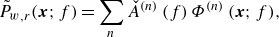 \begin{equation} \tilde {P}_{w,r}({\boldsymbol x};f) = \sum _{n}{\check {A}^{(n)}\left (f\right)\Phi ^{\left (n\right)}\left ({\boldsymbol x};f\right)}, \end{equation}
with $\check {A}^{(n)}(f)=\int \widetilde {P}_{w,r}({\boldsymbol x};f)\Phi ^{(n)}({\boldsymbol x};f)\mathrm{d}{\boldsymbol x}$
being the frequency-dependent complex random expansion coefficients.
$\check {A}^{(n)}(f)=\int \widetilde {P}_{w,r}({\boldsymbol x};f)\Phi ^{(n)}({\boldsymbol x};f)\mathrm{d}{\boldsymbol x}$
being the frequency-dependent complex random expansion coefficients.
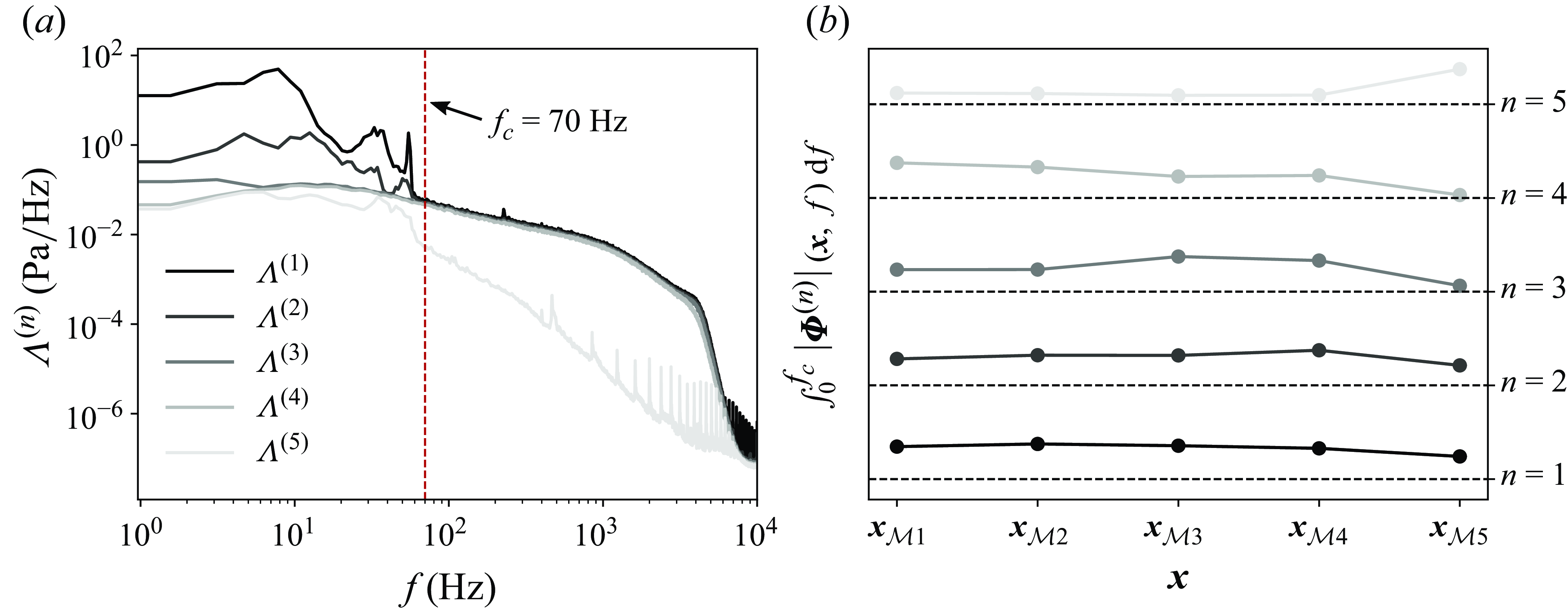
Figure 9. (a) Spectra of the eigenvalue obtained from the complex-valued $\check {R}$
kernel, for test case 3 (
$\check {R}$
kernel, for test case 3 ( $Re_\tau \approx 14\,004$
). (b) Normalised magnitude of the complex modes
$Re_\tau \approx 14\,004$
). (b) Normalised magnitude of the complex modes $\Phi ^{(n)}$
, for
$\Phi ^{(n)}$
, for $n = 1 \ldots 5$
, integrated over the range
$n = 1 \ldots 5$
, integrated over the range $0 \lt f \lesssim 70\,\rm Hz$
. Each curve is offset by one unit vertically for graphical readability.
$0 \lt f \lesssim 70\,\rm Hz$
. Each curve is offset by one unit vertically for graphical readability.
For one of the current datasets (test case 3, $Re_\tau \approx 14\,004$
), the five frequency-dependent eigenvalues are shown in figure 9(a). The first two eigenvalues contain clear signatures of facility noise, especially at the low frequencies. The spectra of the first four eigenvalues show a broadband distribution in the mid-to-high frequency band, whereas the fifth eigenvalue only has significant energy in the low-frequency band at
$Re_\tau \approx 14\,004$
), the five frequency-dependent eigenvalues are shown in figure 9(a). The first two eigenvalues contain clear signatures of facility noise, especially at the low frequencies. The spectra of the first four eigenvalues show a broadband distribution in the mid-to-high frequency band, whereas the fifth eigenvalue only has significant energy in the low-frequency band at $f \lesssim 60\,\rm Hz$
. To determine which mode set to retain for filtering the wall-pressure time series, the spatial distribution of eigenmodes is also examined. In particular, by construction of the experiment, the ideal set of modes to retain consists of those that exhibit no activity at the centreline microphone,
$f \lesssim 60\,\rm Hz$
. To determine which mode set to retain for filtering the wall-pressure time series, the spatial distribution of eigenmodes is also examined. In particular, by construction of the experiment, the ideal set of modes to retain consists of those that exhibit no activity at the centreline microphone, $\mathcal{M}5$
. To aid in the selection of modes, we only consider frequencies in the range
$\mathcal{M}5$
. To aid in the selection of modes, we only consider frequencies in the range $0 \lt f \lt f_c$
, with
$0 \lt f \lt f_c$
, with $f_c = 70\,\rm Hz$
, as the facility noise is concentrated in this band. The magnitude of the eigenmodes, integrated over the aforementioned frequency range, is displayed in figure 9(b). Upon inspection of the five curves, it is clear that modes 3 and 4 are those encompassing negligible activity at the position of the centreline microphone,
$f_c = 70\,\rm Hz$
, as the facility noise is concentrated in this band. The magnitude of the eigenmodes, integrated over the aforementioned frequency range, is displayed in figure 9(b). Upon inspection of the five curves, it is clear that modes 3 and 4 are those encompassing negligible activity at the position of the centreline microphone, ${\boldsymbol x}_{\mathcal{M}5}$
. Based on this, it was decided to reconstruct the wall-pressure time series with modes 3 and 4 only. Therefore, the filtered wall-pressure time series can be computed as the inverse Fourier transform of the frequency-dependent lower-order:
${\boldsymbol x}_{\mathcal{M}5}$
. Based on this, it was decided to reconstruct the wall-pressure time series with modes 3 and 4 only. Therefore, the filtered wall-pressure time series can be computed as the inverse Fourier transform of the frequency-dependent lower-order:
 \begin{equation} \widetilde {P}_{w,f}\left ({\boldsymbol x};f\right) = \sum _{n=\{3,4\}}{\check {A}^{\left (n\right)}\left (f\right)\Phi ^{\left (n\right)}\left ({\boldsymbol x};f\right)}\,\,\,\rightarrow \,\,\,p_{w,f}\left (x,t\right) = \mathcal{F}^{-1}\left [\widetilde {P}_{w,f}({\boldsymbol x};f)\right]. \end{equation}
For the other friction Reynolds numbers considered in this study (see table 1), a similar procedure was applied. Similar conclusions could be drawn in regards to the selection of modes to retain for filtering, with the only minor difference lying in the selection of the upper frequency bound for acoustic contamination, $f_c$
. For increasing Reynolds numbers,
$f_c$
. For increasing Reynolds numbers, $f_c$
increases; physically, this is caused by a larger blade passing frequency of the axial fans operating the pipe flow facility.
$f_c$
increases; physically, this is caused by a larger blade passing frequency of the axial fans operating the pipe flow facility.


 Open access