


1. Introduction
Taylor–Couette (TC) flows typically refer to the fluid motion that occurs between two concentric, coaxial cylinders. Early investigations of these flows aimed to measure fluid viscosity (Mallock Reference Mallock1889, Reference Mallock1896; Couette Reference Couette1890). Associated flow phenomena have attracted considerable attention following the work by Taylor (Reference Taylor1923), which established the critical conditions for the emergence of axial vortices, known as Taylor vortices. Over time, various studies have extensively explored distinct flow patterns and dynamics. The most common geometry involves the inner cylinder rotating while the outer cylinder remains stationary, with several geometric parameters influencing the flow conditions.
The TC flows demonstrate various distinct behaviours influenced by the relative rotation speeds of the cylinders and the fluid properties (Andereck, Liu & Swinney Reference Andereck, Liu and Swinney1986). These flows are instrumental in understanding fundamental phenomena, including the transition from the laminar to the turbulent regime, the emergence of instabilities, and the interactions among various flow regimes (Coles Reference Coles1965; Hristova et al. Reference Hristova, Roch, Schmid and Tuckerman2002; Dou, Khoo & Yeo Reference Dou, Khoo and Yeo2008). At comparatively low rotation rates, the fluid undergoes concentric motions. However, the flow becomes unstable above a critical rotation rate, developing secondary flows and coherent patterns. These vortices result from the interplay between centrifugal forces from the rotation and viscous forces. Andereck et al. (Reference Andereck, Liu and Swinney1986) described various flow regimes present in TC flows, highlighting that standard flow transitions are initiated through bifurcations, leading to distinct flow patterns. Beyond certain critical conditions, flow patterns manifest, with counter-rotating stationary vortices (Taylor vortices) emerging from the primary bifurcations. Secondary bifurcations give rise to time-periodic structures, such as wavy vortex flow, wherein the Taylor vortices oscillate periodically along the axial direction (Strogatz Reference Strogatz2000). Also, particle migration and preferential concentration in TC flow systems have significant implications in engineering, such as particle segregation and filtration (Wereley & Lueptow Reference Wereley and Lueptow1999; Climent, Simonnet & Magnaudet Reference Climent, Simonnet and Magnaudet2007). The TC flows also provide insights into the rheological properties of complex fluids, including polymers (Watanabe, Sumio & Ogata Reference Watanabe, Sumio and Ogata2005; Nicolas & Morozov Reference Nicolas and Morozov2012), suspensions (Majji & Morris Reference Majji and Morris2018; Baroudi et al. Reference Baroudi, Majji, Peluso and Morris2023) and colloids (Yuan & Ronis Reference Yuan and Ronis1993; Ortiz-Ambriz et al. Reference Ortiz-Ambriz, Gerloff, Klapp, Ortín and Tierno2018).
Recently, Wiswell et al. (Reference Wiswell, Snow, Tricouros, Smits and Van Buren2023) examined the influence of gap ratios, identifying shared features with the classical findings of Taylor (Reference Taylor1936). Jeganathan, Alba & Ostilla-Mónico (Reference Jeganathan, Alba and Ostilla-Mónico2023) investigated quasi-axisymmetric structures and the role of the Coriolis parameter, contrasting the two-way coupling in TC flows with the one-way coupling in Rayleigh–Bénard convection. Oishi & Baxter (Reference Oishi and Baxter2023) used a generalised quasi-linear approximation to analyse spiral turbulence (Coles Reference Coles1965), highlighting its connection to the non-normality of the linear operator. Kang et al. (Reference Kang, Yoshikawa, Ntarmouchant, Prigent and Mutabazi2023) demonstrated that large radial temperature gradients destabilise convective cells, inducing a travelling wave pattern through subcritical bifurcation. Also, Crowley et al. (Reference Crowley, Pughe-Sanford, Toler, Grigoriev and Schatz2023) introduced a refined method for examining turbulent intervals, with findings consistent across simulations and experiments, while Alam & Ghosh (Reference Alam and Ghosh2023) proposed a unified scaling for dimensionless torque in neutrally buoyant suspensions of counter-rotating TC flows.
Several studies have examined TC flows in non-circular geometries, uncovering distinct stability characteristics. DiPrima & Stuart (Reference DiPrima and Stuart1972a ,Reference DiPrima and Stuart b ) analysed eccentric configurations using a bi-polar coordinate system, assessing the influence of eccentricity and clearance ratio on flow stability. Esser & Grossmann (Reference Esser and Grossmann1996) derived an analytical stability criterion for TC flows across various radius and speed ratios, while Shu et al. (Reference Shu, Wang, Chew and Zhao2004) demonstrated that eccentricity stabilises Taylor vortices when only the inner cylinder rotates. Oikawa, Karasudani & Funakoshi (Reference Oikawa, Karasudani and Funakoshi1989) employed a Chebyshev–Fourier approach to study the stability of eccentric TC flow, and Mittal, Sidharth & Verma (Reference Mittal, Sidharth and Verma2014) used a finite element framework for global stability analysis. Investigations into combined axial flow and eccentricity effects include the work of Leclercq, Pier & Scott (Reference Leclercq, Pier and Scott2013, Reference Leclercq, Pier and Scott2014), who identified a transition from toroidal Taylor vortices to helical structures at higher eccentricities. Kobine, Mullin & Price (Reference Kobine, Mullin and Price1995) explored TC flow in a stadium-shaped geometry, while Luo et al. (Reference Luo, Zhang, Wang, Cheng and Lyu2023, Reference Luo, Zhang, Cheng and Lyu2024) studied TC flows with three-lobe multi-wedge clearance, noting delayed transition due to separation bubbles, and the emergence of unique vortical structures. Also, several studies have addressed the stability of TC systems under heating and gravitational effects (e.g. Eagles & Soundalgekar Reference Eagles and Soundalgekar1997; Kedia, Hunt & Colonius Reference Kedia, Hunt and Colonius1998; White & Muller Reference White and Muller2000; Al-Mubaiyedh, Sureshkumar & Khomami Reference Al-Mubaiyedh, Sureshkumar and Khomami2002; Jenny & Nsom Reference Jenny and Nsom2007).
Early numerical studies by Lewis (Reference Lewis1979) demonstrated that increasing the gap between cylinders in square enclosures weakens corner eddies. Mullin & Lorenzen (Reference Mullin and Lorenzen1985) examined transitions between four-cell and six-cell states, identifying geometric asymmetries that led to time-dependent behaviour, distinguishing square-enclosed TC flow from its circular counterpart. Kobine & Mullin (Reference Kobine and Mullin1994) and Kobine et al. (Reference Kobine, Mullin and Price1995) extended this analysis to finite length effects, showing that anomalous 40-cell states remained disconnected from the primary flow up to 2.7 times the critical Reynolds number, with stability primarily dictated by end cells rather than cylinder length. Their findings highlighted the sensitivity of TC flows to both geometry and boundary effects. The present study builds on these insights by investigating vortex interactions and turbulence modulation within a square enclosure, providing a detailed analysis under various scenarios.

Figure 1. Basic schematic illustrating possible types of vortices in the TC system with square enclosure: (a) Taylor vortices driven by centrifugal instability, (b) Görtler vortices induced by curvature effects near the concave boundaries, (c) separation regions forming near the enclosure walls, and (d) Moffatt vortices appearing at the corners due to secondary flow effects. The cross-section A–A’ indicates the spatial distribution of these vortices along the radial and vertical directions.
In general, TC flow in non-canonical systems typically features various types of vortices. Taylor vortices, which are prevalent in both steady and periodic flow regimes, arise from centrifugal instabilities. Görtler vortices, occurring at relatively high Reynolds numbers, are often linked to the route to turbulence (Floryan Reference Floryan1991; Saric et al. Reference Saric1994). These vortices develop due to the convex curvature of the inner surface of the cylinder, and are observed primarily in the radial outflow region between Taylor cells. Similarly, vortices may also form as a result of flow separation near the venturi-like cross-section, or at the corner region of the square enclosure. In the presence of sharp corners, the formation of Moffatt vortices is also likely. While there may be additional paths of eddy formation within the flow field that have yet to be analysed, Moffatt vortices – which form in corners – are the exception among these four types. Figure 1 shows a basic schematic illustrating these distinct vortex types.
Various complex interactions may occur in TC flows within square enclosures, potentially expanding upon the insights from Mullin & Lorenzen (Reference Mullin and Lorenzen1985). Their experiments primarily targeted lower Reynolds numbers and used variable height configurations to study aspect ratio effects. At higher Reynolds numbers, new flow structures emerge, leading to a critical area for further research. Also, the influence of the gap size between the rotating cylinders on flow instability and vortex dynamics remains underexplored. A linear stability analysis of this geometry could offer insights into transition mechanisms, particularly at higher Reynolds numbers, uncovering new flow behaviours.
In this study, we explore various turbulence conditions, with emphasis on the dynamics of turbulent Taylor vortices. Specifically, the dominant coherent motions and the modulation of the inner–outer wall gap were examined with various gap ratios and Reynolds numbers spanning an order of magnitude. Although the parameter space is vast, the selected conditions provide a critical understanding of the flow dynamics under these distinct conditions. The experimental set-up is described in § 2, the results are provided in § 3, a discussion is given in § 4, and key conclusions are summarised in § 5. Also, a linear stability analysis using a meshless numerical approach (Shahane, Radhakrishnan & Vanka Reference Shahane, Radhakrishnan and Vanka2021; Unnikrishnan et al. Reference Unnikrishnan, Narayanan and Vanka2024b ), is included in Appendix B.
2. Experimental set-up
Three distinct TC systems, each with outer square enclosures, were constructed using 4.8 mm thick transparent acrylic sheets. The systems shared a concentric rotating inner cylinder with diameter $d=80$
mm and height
$d=80$
mm and height $H=450$
mm, while the square cross-section enclosures had sides 90 mm, 100 mm and 120 mm. These values resulted in minimum gaps between the outer enclosure and inner cylinder
$H=450$
mm, while the square cross-section enclosures had sides 90 mm, 100 mm and 120 mm. These values resulted in minimum gaps between the outer enclosure and inner cylinder $\varDelta =5$
, 10 and 20 mm, or gap ratios
$\varDelta =5$
, 10 and 20 mm, or gap ratios $\varDelta /d=1/16$
, 1/8 and 1/4. The associated slenderness ratio, defined as the ratio of the tank’s height to the minimum gap between the cylinder and the square walls, was
$\varDelta /d=1/16$
, 1/8 and 1/4. The associated slenderness ratio, defined as the ratio of the tank’s height to the minimum gap between the cylinder and the square walls, was $H/\varDelta =90$
, 45 and 22.5. A higher slenderness ratio is preferable as it reduces the impact of end effects of the tank on the flow features within the observation area. The inner cylinder was affixed to a steel shaft with diameter 5 mm, which in turn was connected to a stepper motor mounted coaxially. This motor was installed atop the stationary square tank. A small clearance of 2 mm between the rotating cylinder and square tank was left at the bottom and top to prevent contact and potential wear.
$H/\varDelta =90$
, 45 and 22.5. A higher slenderness ratio is preferable as it reduces the impact of end effects of the tank on the flow features within the observation area. The inner cylinder was affixed to a steel shaft with diameter 5 mm, which in turn was connected to a stepper motor mounted coaxially. This motor was installed atop the stationary square tank. A small clearance of 2 mm between the rotating cylinder and square tank was left at the bottom and top to prevent contact and potential wear.
Characterisation of the flow within the TC systems was conducted by varying the angular velocity of the inner cylinder, with $\Omega$
ranging from
$\Omega$
ranging from $2\unicode{x03C0} /5$
to
$2\unicode{x03C0} /5$
to $2\unicode{x03C0}\ \text{rad}\ \text{s}^{-1}$
(12, 24, 36, 48 and 60 revolutions per minute, rpm). This range enabled the exploration of Reynolds numbers based on the minimum gap, spanning an order of magnitude from
$2\unicode{x03C0}\ \text{rad}\ \text{s}^{-1}$
(12, 24, 36, 48 and 60 revolutions per minute, rpm). This range enabled the exploration of Reynolds numbers based on the minimum gap, spanning an order of magnitude from $Re_{\varDelta } = [\Omega r_0] \times \varDelta / \nu = 230$
to
$Re_{\varDelta } = [\Omega r_0] \times \varDelta / \nu = 230$
to $4.6 \times 10^3$
, capturing the shear-dominated dynamics within the gap region. Given the azimuthal variability in the gap, leading to changes in mean shear and pressure gradient, we also consider the Reynolds number based on the inner radius. This alternative definition has been used in studies with similar outer square cross-section configurations, such as Mullin & Lorenzen (Reference Mullin and Lorenzen1985) and Kobine & Mullin (Reference Kobine and Mullin1994), to investigate low-dimensional bifurcation phenomena. In alignment with these studies, we report Reynolds numbers based on the inner radius, spanning
$4.6 \times 10^3$
, capturing the shear-dominated dynamics within the gap region. Given the azimuthal variability in the gap, leading to changes in mean shear and pressure gradient, we also consider the Reynolds number based on the inner radius. This alternative definition has been used in studies with similar outer square cross-section configurations, such as Mullin & Lorenzen (Reference Mullin and Lorenzen1985) and Kobine & Mullin (Reference Kobine and Mullin1994), to investigate low-dimensional bifurcation phenomena. In alignment with these studies, we report Reynolds numbers based on the inner radius, spanning $Re = [\Omega r_0] \times r_0 / \nu = 1.8 \times 10^3$
to
$Re = [\Omega r_0] \times r_0 / \nu = 1.8 \times 10^3$
to $9.1 \times 10^3$
. To mitigate the formation of bubbles caused by dissolved oxygen in the water, the fluid was preheated prior to being introduced into the square cylinder. The tank was then allowed to cool overnight, ensuring that the fluid reached ambient temperature 25
$9.1 \times 10^3$
. To mitigate the formation of bubbles caused by dissolved oxygen in the water, the fluid was preheated prior to being introduced into the square cylinder. The tank was then allowed to cool overnight, ensuring that the fluid reached ambient temperature 25 $^\circ$
C before conducting the experiments.
$^\circ$
C before conducting the experiments.
The experiments used a Nema 23 stepper motor with maximum holding torque 3 Nm and 200 steps per revolution, yielding resolution 1.8 $^\circ$
per step. This motor was driven by an Arduino board paired with a DM566T stepper driver module. A 10 min period was allotted for the flow to stabilise before initiating measurements, with a tachometer employed to verify the motor’s speed, ensuring the specified rpm setting. Flow field characterisation around the mid-height of the system was achieved through particle image velocimetry, using a 2 MP CMOS camera. The field of view was centred vertically on the cylinder and aligned with the radial section corresponding to the minimum radial gap. For cases with
$^\circ$
per step. This motor was driven by an Arduino board paired with a DM566T stepper driver module. A 10 min period was allotted for the flow to stabilise before initiating measurements, with a tachometer employed to verify the motor’s speed, ensuring the specified rpm setting. Flow field characterisation around the mid-height of the system was achieved through particle image velocimetry, using a 2 MP CMOS camera. The field of view was centred vertically on the cylinder and aligned with the radial section corresponding to the minimum radial gap. For cases with $\varDelta /d=1/4, 1/8$
, the field of view spanned vertically approximately 70 mm, and for
$\varDelta /d=1/4, 1/8$
, the field of view spanned vertically approximately 70 mm, and for $\varDelta /d=1/16$
, it covered around 40 mm. Data were captured over duration 100 s, adjusting frame rate between 100 Hz and 300 Hz.
$\varDelta /d=1/16$
, it covered around 40 mm. Data were captured over duration 100 s, adjusting frame rate between 100 Hz and 300 Hz.
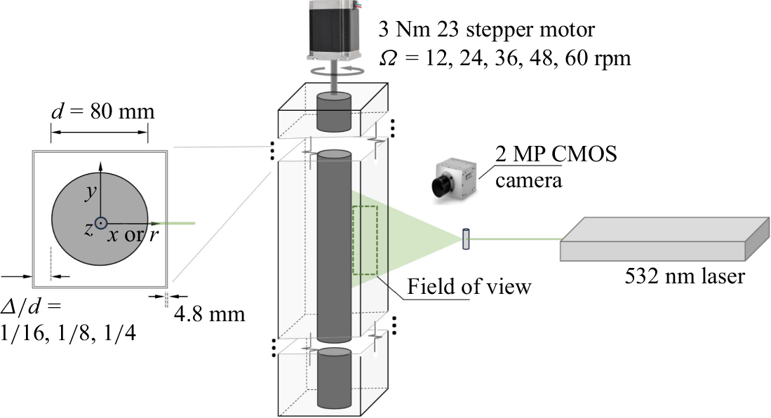
Figure 2. Schematic of the TC system with outer square cylinder illustrating the parameter range for the gap $\varDelta /d$
, and rotational velocity of the inner cylinder
$\varDelta /d$
, and rotational velocity of the inner cylinder $\Omega _i$
.
$\Omega _i$
.
3. Results
Characterising vortices in the turbulent regime is challenging due to the coexistence of vortices with varying strengths and scales. There are various vortex identification techniques (e.g. Jeong & Hussain Reference Jeong and Hussain1995; Dubief & Delcayre Reference Dubief and Delcayre2000; Chu & Laurien Reference Chu and Laurien2016). Here, we use the approach proposed by Graftieaux, Michard & Grosjean (Reference Graftieaux, Michard and Grosjean2001), who introduced the function $\Gamma _1$
for vortex centre identification. For an axisymmetric vortex,
$\Gamma _1$
for vortex centre identification. For an axisymmetric vortex, $\Gamma _1$
is bounded by 1 and peaks at the vortex centre, given by
$\Gamma _1$
is bounded by 1 and peaks at the vortex centre, given by
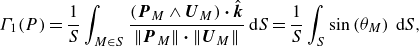 \begin{equation} \Gamma _1(P)=\frac {1}{S} \int _{M \in S} \frac {\left (\boldsymbol{P}_M \wedge \boldsymbol{U}_M\right ) \boldsymbol{\cdot} \hat{\boldsymbol{k}}}{\|\boldsymbol{P}_M\| \boldsymbol{\cdot} \left \|\boldsymbol{U}_M\right \|}\, \mathrm{d} S=\frac {1}{S} \int _S \sin \left (\theta _M\right )\, \mathrm{d} S, \end{equation}
where $P$
represents the point under examination,
$P$
represents the point under examination, $M$
is any point within the two-dimensional region
$M$
is any point within the two-dimensional region $S$
surrounding
$S$
surrounding $P$
,
$P$
, $\hat{\boldsymbol{k}}$
is the unit vector perpendicular to
$\hat{\boldsymbol{k}}$
is the unit vector perpendicular to $S$
, and
$S$
, and $\theta _M$
is the angle between the position vector
$\theta _M$
is the angle between the position vector $\boldsymbol{P}_M$
and the velocity vector
$\boldsymbol{P}_M$
and the velocity vector $\boldsymbol{U}_M$
at
$\boldsymbol{U}_M$
at ${M}$
.
${M}$
.
To analyse vortex dynamics, we first tracked the motion of identified vortex centres across consecutive frames within a radius of three times the vector resolution. Connecting these centres across frames yielded distinct vortex trajectories. A Gaussian filter spanning five frames (0.05 s) was applied to enhance clarity and reduce noise.
Figure 3 illustrates the vertical motion projections of a dominant vortex for various gap sizes $\varDelta /d$
and Reynolds numbers
$\varDelta /d$
and Reynolds numbers $Re$
. This figure highlights the influence of
$Re$
. This figure highlights the influence of $Re$
on vortex oscillatory motions. At lower Reynolds numbers (figure 3
a), vortex motion remains relatively steady with minor fluctuations. As
$Re$
on vortex oscillatory motions. At lower Reynolds numbers (figure 3
a), vortex motion remains relatively steady with minor fluctuations. As $Re$
increases to
$Re$
increases to $6 \times 10^3$
(figure 3
b), vertical motions become more pronounced, indicating unsteady loading from turbulence. At
$6 \times 10^3$
(figure 3
b), vertical motions become more pronounced, indicating unsteady loading from turbulence. At $Re = 10^4$
(figure 3
c), the vortex motion exhibits significant fluctuations, particularly in smaller gaps (
$Re = 10^4$
(figure 3
c), the vortex motion exhibits significant fluctuations, particularly in smaller gaps ( $\varDelta /d=1/8$
and
$\varDelta /d=1/8$
and $1/16$
), where irregular and rapid position changes suggest enhanced turbulence and vortex interactions. Vortex motion remains more regular and stable in larger gaps, even at higher Reynolds numbers. For additional insight, Appendix A presents related figures for cases sharing the same
$1/16$
), where irregular and rapid position changes suggest enhanced turbulence and vortex interactions. Vortex motion remains more regular and stable in larger gaps, even at higher Reynolds numbers. For additional insight, Appendix A presents related figures for cases sharing the same $Re_{\varDelta }$
. Interestingly, vortex motion exhibits distinct behaviour when compared at the same
$Re_{\varDelta }$
. Interestingly, vortex motion exhibits distinct behaviour when compared at the same $Re_{\varDelta }$
with different minimum gap sizes
$Re_{\varDelta }$
with different minimum gap sizes $\varDelta /d$
, suggesting that the strong variability in the mean shear gradient – resulting from azimuthal gap variations – plays a key role in shaping vortex dynamics.
$\varDelta /d$
, suggesting that the strong variability in the mean shear gradient – resulting from azimuthal gap variations – plays a key role in shaping vortex dynamics.
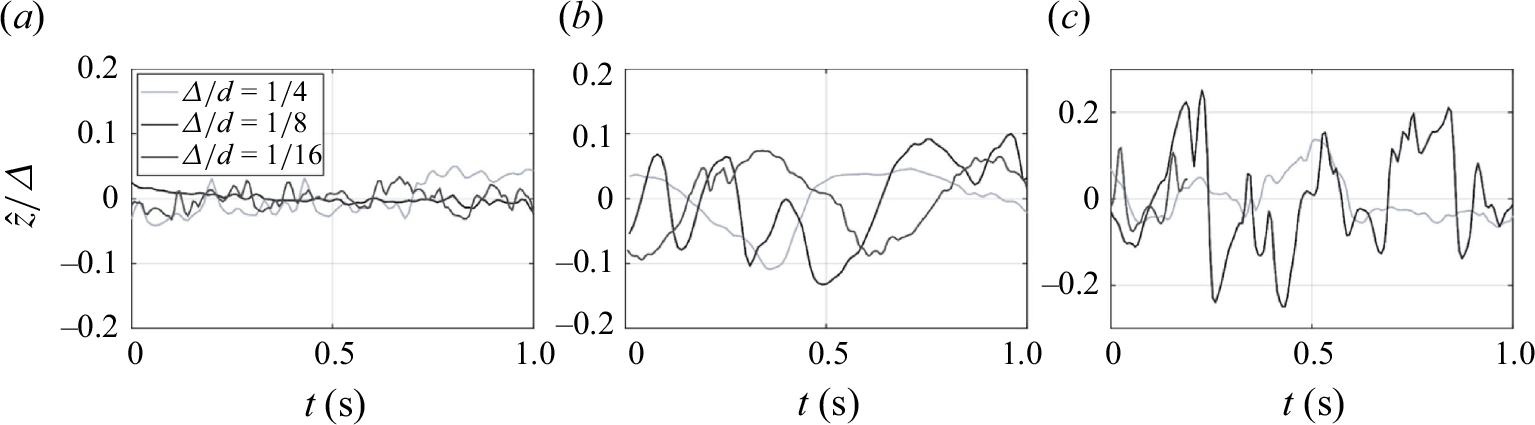
Figure 3. Vertical motions of a dominant vortex in the $\varDelta /d=1/4$
, 1/8 and 1/16 scenarios under approximate
$\varDelta /d=1/4$
, 1/8 and 1/16 scenarios under approximate $Re$
values (a)
$Re$
values (a) $2\times 10^3$
, (b)
$2\times 10^3$
, (b) $6\times 10^3$
and (c)
$6\times 10^3$
and (c) $10^4$
. Refer to the figure 20 in Appendix A for cases with shared
$10^4$
. Refer to the figure 20 in Appendix A for cases with shared $Re_{\varDelta }$
.
$Re_{\varDelta }$
.
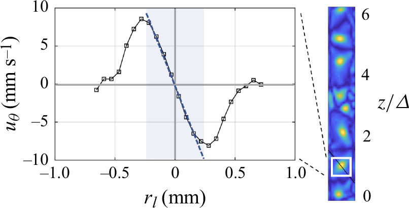
Figure 4. Instantaneous tangential velocity profile about the centre of a vortex from the $\Gamma$
function contour in the
$\Gamma$
function contour in the $\varDelta /d = 1/8$
case at
$\varDelta /d = 1/8$
case at $Re \approx 2\times 10^3$
. The light blue contour highlights the vortex core.
$Re \approx 2\times 10^3$
. The light blue contour highlights the vortex core.
Vortex characterisation was performed using a conventional approach that defines the vortex core as a region with solid body rotation (Hamed, Jin & Chamorro Reference Hamed, Jin and Chamorro2015). After identifying vortex centres using the $\Gamma _1$
function, the asymmetry of each vortex was assessed by analysing its major and minor axes. This analysis was conducted using the eigenvectors of the covariance matrix, computed from the positions of points where
$\Gamma _1$
function, the asymmetry of each vortex was assessed by analysing its major and minor axes. This analysis was conducted using the eigenvectors of the covariance matrix, computed from the positions of points where $\Gamma _1$
exceeded a predefined threshold, to establish the vortex axes. To refine the analysis, the velocity data were interpolated along these axes using spline interpolation, allowing for a detailed examination of the velocity distribution around the vortex centres. Figure 4 presents the tangential velocity profile along a radial line across the centre of a vortex for a configuration with gap width
$\Gamma _1$
exceeded a predefined threshold, to establish the vortex axes. To refine the analysis, the velocity data were interpolated along these axes using spline interpolation, allowing for a detailed examination of the velocity distribution around the vortex centres. Figure 4 presents the tangential velocity profile along a radial line across the centre of a vortex for a configuration with gap width $\varDelta /d=1/8$
at
$\varDelta /d=1/8$
at $Re=2\times 10^3$
. The light blue contour delineates the vortex core, illustrating the tangential velocity variation, and confirming the assumption of solid body rotation within the core region.
$Re=2\times 10^3$
. The light blue contour delineates the vortex core, illustrating the tangential velocity variation, and confirming the assumption of solid body rotation within the core region.
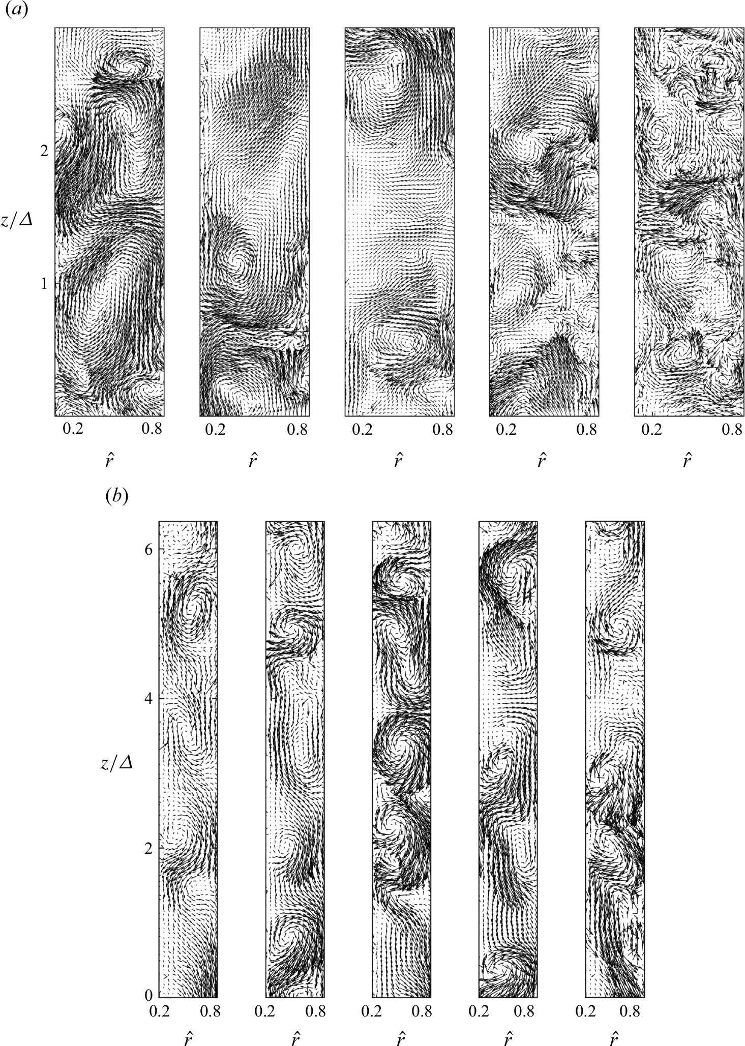
Figure 5. Instantaneous in-plane flow field for gap sizes (a) $\varDelta /d=1/4$
and (b)
$\varDelta /d=1/4$
and (b) $\varDelta /d=1/16$
, with increasing Reynolds number from left to right (
$\varDelta /d=1/16$
, with increasing Reynolds number from left to right ( $Re=2\times 10^3$
,
$Re=2\times 10^3$
, $4\times 10^3$
,
$4\times 10^3$
, $6\times 10^3$
,
$6\times 10^3$
, $8\times 10^3$
,
$8\times 10^3$
, $10^4$
).
$10^4$
).
Instantaneous velocity fields presented in figure 5 reveal distinct flow patterns that vary significantly in the different scenarios. From here on, the normalised radial coordinate is defined as $\hat {r} = (r - r_i)/\varDelta$
, where
$\hat {r} = (r - r_i)/\varDelta$
, where $\hat {r} = 0$
corresponds to the cylinder surface, and
$\hat {r} = 0$
corresponds to the cylinder surface, and $\hat {r} = 1$
represents the outer rectangular enclosure, all referred to the minimum gap. At a lower Reynolds number, the velocity fields exhibit well-defined Taylor vortices for narrower gaps, consistent with the classical flow structure of TC systems. As the gap size increases, smaller vortices emerge alongside the dominant Taylor cells, causing their deformation, and amplifying velocity fluctuations.
$\hat {r} = 1$
represents the outer rectangular enclosure, all referred to the minimum gap. At a lower Reynolds number, the velocity fields exhibit well-defined Taylor vortices for narrower gaps, consistent with the classical flow structure of TC systems. As the gap size increases, smaller vortices emerge alongside the dominant Taylor cells, causing their deformation, and amplifying velocity fluctuations.
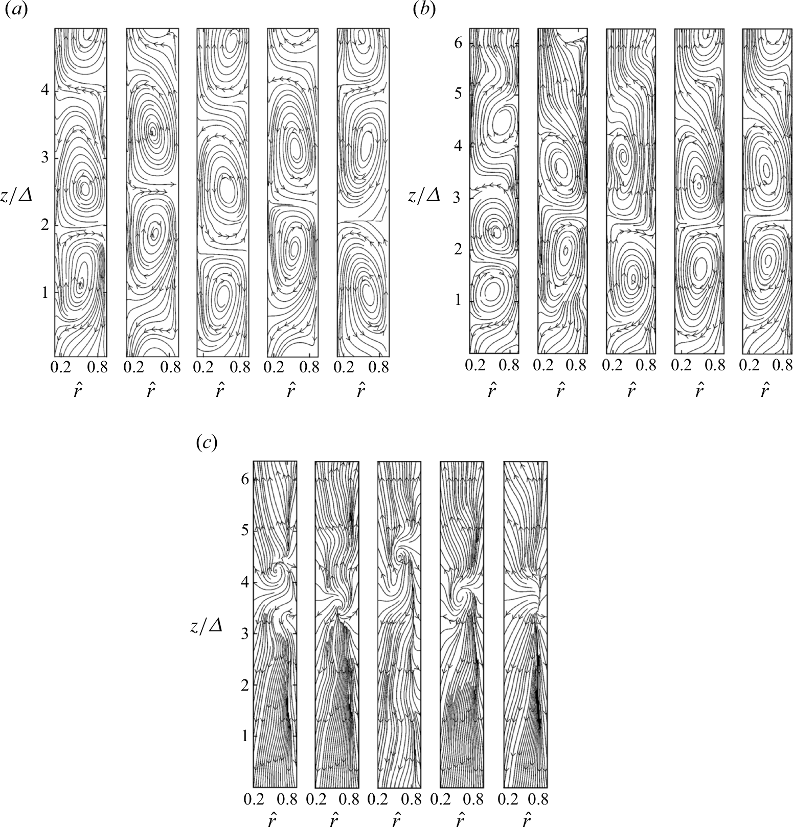
Figure 6. In-plane streamlines for gap sizes (a) $\varDelta /d=1/4$
, (b)
$\varDelta /d=1/4$
, (b) $\varDelta /d=1/8$
and (c)
$\varDelta /d=1/8$
and (c) $\varDelta /d=1/16$
, progressing from left to right with
$\varDelta /d=1/16$
, progressing from left to right with $Re=2\times 10^3$
,
$Re=2\times 10^3$
, $4\times 10^3$
,
$4\times 10^3$
, $6\times 10^3$
,
$6\times 10^3$
, $8\times 10^3$
,
$8\times 10^3$
, $10^4$
.
$10^4$
.
The in-plane streamlines presented in figure 6 provide further insight into the bulk flow structures across different gap sizes. In general, for the largest gap case ( $\varDelta /d=1/4$
), the mean flow exhibits Taylor vortices with a skewed-oval shape, likely due to the influence of the square enclosure imposing geometric constraints on the vortex formation. While the overall structure remains consistent, the aspect ratio of these Taylor cells appears to be influenced by the proximity of the outer square walls. In the intermediate gap scenario (
$\varDelta /d=1/4$
), the mean flow exhibits Taylor vortices with a skewed-oval shape, likely due to the influence of the square enclosure imposing geometric constraints on the vortex formation. While the overall structure remains consistent, the aspect ratio of these Taylor cells appears to be influenced by the proximity of the outer square walls. In the intermediate gap scenario ( $\varDelta /d=1/8$
), the Taylor vortices retain their fundamental structure, but their count within a given axial span varies with Reynolds number. The spatial extent of these mean flow Taylor cells scales with the gap size, with each counter-rotating vortex pair spanning approximately 3–4 times the gap width
$\varDelta /d=1/8$
), the Taylor vortices retain their fundamental structure, but their count within a given axial span varies with Reynolds number. The spatial extent of these mean flow Taylor cells scales with the gap size, with each counter-rotating vortex pair spanning approximately 3–4 times the gap width $\varDelta$
. At higher Reynolds numbers, subtle modulations in the streamlines suggest the increasing presence of smaller-scale vortices, which interact with the dominant Taylor cells, leading to the emergence of wave-like distortions. These perturbations indicate a transition towards a more dynamically modulated flow, where smaller vortices begin to influence the large-scale structures.
$\varDelta$
. At higher Reynolds numbers, subtle modulations in the streamlines suggest the increasing presence of smaller-scale vortices, which interact with the dominant Taylor cells, leading to the emergence of wave-like distortions. These perturbations indicate a transition towards a more dynamically modulated flow, where smaller vortices begin to influence the large-scale structures.
For the smallest gap case ( $\varDelta /d=1/16$
), figure 6(c) reveals a markedly different behaviour. The Taylor cell structures become increasingly irregular and less dominant across the vertical span, suggesting a loss of coherence in their organisation. This behaviour likely arises due to the strongest mean shear gradient imposed by the narrow gap, which amplifies small-scale fluctuations and suppresses the formation of well-defined Taylor vortices. As
$\varDelta /d=1/16$
), figure 6(c) reveals a markedly different behaviour. The Taylor cell structures become increasingly irregular and less dominant across the vertical span, suggesting a loss of coherence in their organisation. This behaviour likely arises due to the strongest mean shear gradient imposed by the narrow gap, which amplifies small-scale fluctuations and suppresses the formation of well-defined Taylor vortices. As $Re$
increases, these irregular structures are further disrupted by turbulence, reinforcing the trend towards more disorganised, less stable flow patterns.
$Re$
increases, these irregular structures are further disrupted by turbulence, reinforcing the trend towards more disorganised, less stable flow patterns.

Figure 7. Space–time features of the radial velocity parallel to the system axis at $\hat {r}=0.5$
for Reynolds numbers
$\hat {r}=0.5$
for Reynolds numbers $Re=2\times 10^3$
,
$Re=2\times 10^3$
, $4\times 10^3$
and
$4\times 10^3$
and $8\times 10^3$
, and gaps
$8\times 10^3$
, and gaps $\varDelta /d=1/4$
, 1/8 and 1/16. The white-dashed boxes at
$\varDelta /d=1/4$
, 1/8 and 1/16. The white-dashed boxes at $\varDelta /d = 1/4$
and 1/8 for
$\varDelta /d = 1/4$
and 1/8 for $Re=2\times 10^3$
highlight vortex break-up and reconnection instance later described in figures 8 and 9.
$Re=2\times 10^3$
highlight vortex break-up and reconnection instance later described in figures 8 and 9.
The space–time evolution of the radial velocity at $\hat {r}=0.5$
, parallel to the axis, is shown in figure 7 for selected cases. This visualisation highlights the temporal persistence and regularity of Taylor vortices and their dependence on both
$\hat {r}=0.5$
, parallel to the axis, is shown in figure 7 for selected cases. This visualisation highlights the temporal persistence and regularity of Taylor vortices and their dependence on both $Re$
and
$Re$
and $\varDelta$
. The degree of regularity in Taylor cell structures reduces with increasing
$\varDelta$
. The degree of regularity in Taylor cell structures reduces with increasing $Re$
and decreasing gap size, highlighting the limitations of characterising the flow using either
$Re$
and decreasing gap size, highlighting the limitations of characterising the flow using either $Re$
or
$Re$
or $Re_{\varDelta }$
alone. Specifically, while
$Re_{\varDelta }$
alone. Specifically, while $Re$
does not explicitly account for the influence of gap size,
$Re$
does not explicitly account for the influence of gap size, $Re_{\varDelta }$
does not fully capture the continuous variation in the mean shear gradient across different configurations. Appendix A further illustrates key differences at shared
$Re_{\varDelta }$
does not fully capture the continuous variation in the mean shear gradient across different configurations. Appendix A further illustrates key differences at shared $Re_{\varDelta }$
values. Also, figure 7 reveals several key dynamic processes, including vortex breakdown and reconnection, deformation, variations in vortex lifespan, turbulence-induced fluctuations, and axial variability across different time scales. The emergence of irregular motions at higher
$Re_{\varDelta }$
values. Also, figure 7 reveals several key dynamic processes, including vortex breakdown and reconnection, deformation, variations in vortex lifespan, turbulence-induced fluctuations, and axial variability across different time scales. The emergence of irregular motions at higher $Re$
and smaller
$Re$
and smaller $\varDelta$
further reinforces the role of geometric confinement and shear-induced instabilities in modulating the flow.
$\varDelta$
further reinforces the role of geometric confinement and shear-induced instabilities in modulating the flow.
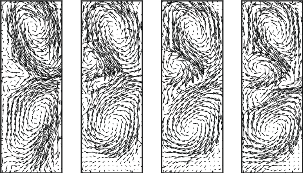
Of particular relevance are vortex oscillations, which are examined next to elucidate the underlying mechanisms governing these behaviours. Figure 8 presents a few consecutive images capturing the interactions between Görtler and Taylor vortices with both opposite and identical rotational senses. In general, counter-rotating vortices tend to elongate and eventually break up, whereas co-rotating vortices exhibit a tendency to merge, though this process remains inconsistent. Görtler vortices typically form in pairs along the surface of the inner circular cylinder, particularly at the radial outflow boundaries between Taylor cells. These outflows facilitate the transport of vortices towards the outer square enclosure, where they may evolve into new Taylor cells by extracting energy from the surrounding flow.
Regarding vortex formation mechanisms, Görtler vortices initially remain stable when positioned between counter-rotating Taylor cells. However, this stability is susceptible to minor perturbations that induce shear forces, leading to uneven stretching, splitting, and potential merging of the vortices. Extended sequences indicate that vortices in contact generally exhibit opposite rotation. However, perturbations can occasionally facilitate interactions between Görtler vortices and Taylor cells rotating in the same direction, potentially leading to vortex merging. While Görtler vortices may contribute to the formation of new Taylor cells, Taylor cells tend to maintain their structure at lower Reynolds numbers due to their inherent stability. For a broader discussion on vortex interactions, see Dritschel (Reference Dritschel1995) and Saffman & Baker (Reference Saffman and Baker1979). Also, supplementary movie 1 provides a visualisation of interactions where new Taylor cells emerge from Görtler vortices.
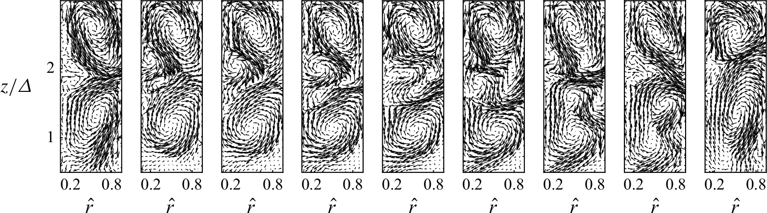
Figure 8. Consecutive instantaneous in-plane velocity vectors indicating the mechanism of formation of Taylor cells from the Görtler cells to replace the existing Taylor vortices. The total time representing this series of frames is approximately 6 s. The case presented here is for the gap $\varDelta /d=1/4$
and
$\varDelta /d=1/4$
and $Re = 2\times 10^3$
.
$Re = 2\times 10^3$
.
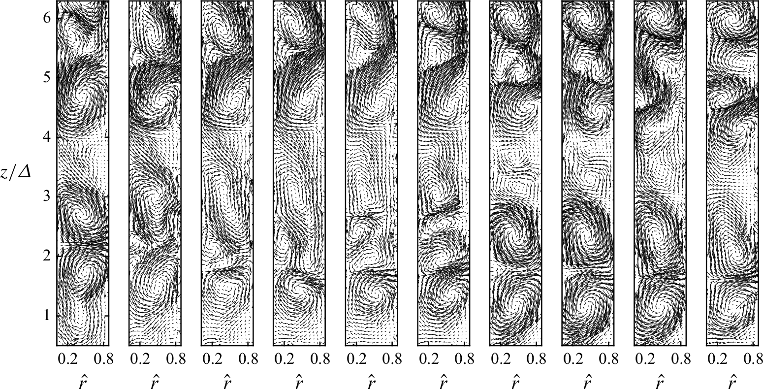
Figure 9. Consecutive instantaneous in-plane velocity vectors indicating the mechanism of formation of a new set of Taylor cells from the Görtler cells. The total time representing this series is approximately 5 s. The case presented here is for the gap $\varDelta /d=1/8$
and
$\varDelta /d=1/8$
and $Re = 2\times 10^3$
.
$Re = 2\times 10^3$
.
Another distinctive mechanism is observed in the sequential images of figure 9 ( $\varDelta /d=1/8$
,
$\varDelta /d=1/8$
, $Re = 2\times 10^3$
), which captures a switching process between two distinct sets of cell structures. In this process, Görtler vortices evolve into a new set of Taylor cells without merging with the pre-existing ones. As a result, the number of Taylor cells increases in the vertical direction while maintaining a constrained axial length, forming smaller-scale Taylor vortices. This behaviour suggests the coexistence of multiple Taylor cell scales within the system. Similar switching dynamics and the presence of multiple Taylor cells were previously documented by Mullin & Lorenzen (Reference Mullin and Lorenzen1985), reinforcing the complex interplay of vortex interactions in TC flows. A complementary visualisation of this phenomenon is provided in supplementary movie 2.
$Re = 2\times 10^3$
), which captures a switching process between two distinct sets of cell structures. In this process, Görtler vortices evolve into a new set of Taylor cells without merging with the pre-existing ones. As a result, the number of Taylor cells increases in the vertical direction while maintaining a constrained axial length, forming smaller-scale Taylor vortices. This behaviour suggests the coexistence of multiple Taylor cell scales within the system. Similar switching dynamics and the presence of multiple Taylor cells were previously documented by Mullin & Lorenzen (Reference Mullin and Lorenzen1985), reinforcing the complex interplay of vortex interactions in TC flows. A complementary visualisation of this phenomenon is provided in supplementary movie 2.
The distinct vortex dynamics in these systems lead to energy redistribution across different scales, which is examined through spectral distributions. Figure 10 presents the compensated spectra of the axial velocity component at radial position $\hat {r} = 0.5$
, for
$\hat {r} = 0.5$
, for $Re = 8\times 10^3$
and
$Re = 8\times 10^3$
and $10^4$
. The spectra are averaged along the axial direction and are compared across three different gap ratios,
$10^4$
. The spectra are averaged along the axial direction and are compared across three different gap ratios, $\varDelta /d = 1/4$
, 1/8 and 1.16. In figure 10(a), at
$\varDelta /d = 1/4$
, 1/8 and 1.16. In figure 10(a), at $Re = 8\times 10^3$
, the compensated spectra show that the energy distribution across scales is influenced by the gap ratio. The
$Re = 8\times 10^3$
, the compensated spectra show that the energy distribution across scales is influenced by the gap ratio. The $\varDelta /d =1/4$
case exhibits a broader peak at lower frequencies, approximately associated with integral scales, indicating the presence of larger coherent structures. The
$\varDelta /d =1/4$
case exhibits a broader peak at lower frequencies, approximately associated with integral scales, indicating the presence of larger coherent structures. The $\varDelta /d = 1/8$
and
$\varDelta /d = 1/8$
and $1/16$
cases show a shift of energy towards higher frequencies, suggesting the dominance of smaller-scale structures induced by the restricted space. In figure 10(b), at
$1/16$
cases show a shift of energy towards higher frequencies, suggesting the dominance of smaller-scale structures induced by the restricted space. In figure 10(b), at $Re = 10^4$
, the energy distribution across all scales increases, as evidenced by the higher peaks in the spectra compared to the
$Re = 10^4$
, the energy distribution across all scales increases, as evidenced by the higher peaks in the spectra compared to the $Re = 8\times 10^3$
case. This increase in energy at higher frequencies indicates enhanced turbulence levels. The
$Re = 8\times 10^3$
case. This increase in energy at higher frequencies indicates enhanced turbulence levels. The $\varDelta /d = 1/4$
gap again shows a prominent peak at lower frequencies, but the spectra for
$\varDelta /d = 1/4$
gap again shows a prominent peak at lower frequencies, but the spectra for $\varDelta /d = 1/8$
and
$\varDelta /d = 1/8$
and $1/16$
now display a more pronounced energy presence at even higher frequencies.
$1/16$
now display a more pronounced energy presence at even higher frequencies.
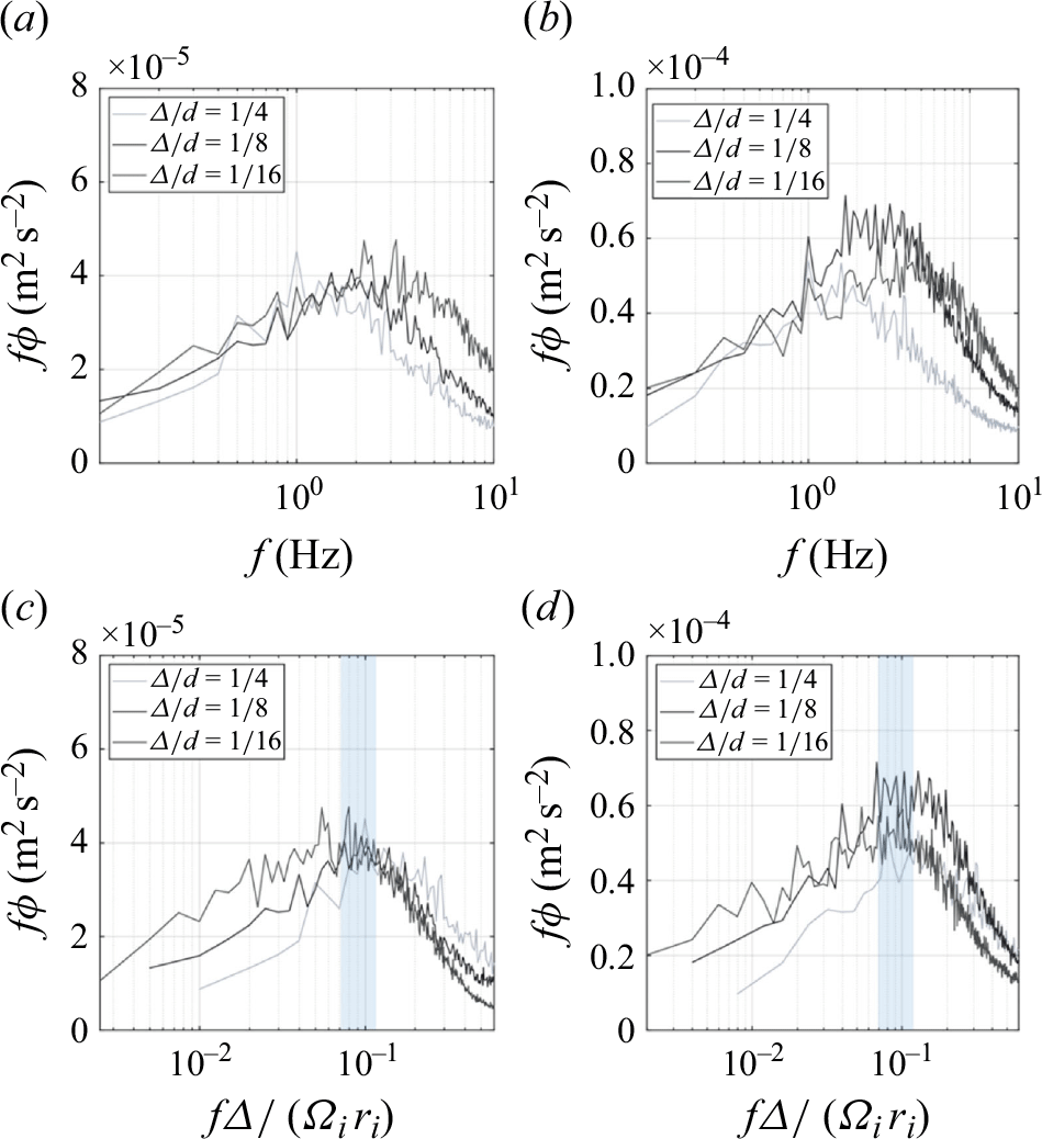
Figure 10. Compensated spectra of the axial velocity component, averaged along the axial direction at $\hat {r} = 0.5$
for various gap ratios
$\hat {r} = 0.5$
for various gap ratios $\varDelta /d=1/4$
,
$\varDelta /d=1/4$
, $1/8$
and
$1/8$
and $1/16$
: (a)
$1/16$
: (a) $Re = 8\times 10^3$
, (b)
$Re = 8\times 10^3$
, (b) $Re = 10^4$
, (c) counterpart of
$Re = 10^4$
, (c) counterpart of $Re = 8\times 10^3$
with reduced frequency, (d) counterpart of
$Re = 8\times 10^3$
with reduced frequency, (d) counterpart of $Re = 10^4$
with reduced frequency.
$Re = 10^4$
with reduced frequency.
It is worth highlighting a tendency to maintain energy at lower frequencies due to the dominance of larger vortices, which is evidenced by the comparatively similar spectral distribution at scales larger than $f\approx 2$
Hz for the
$f\approx 2$
Hz for the $Re=8\times 10^3$
case, and
$Re=8\times 10^3$
case, and $f\approx 1$
Hz for the
$f\approx 1$
Hz for the $Re=10^4$
case. In contrast, smaller gaps and higher Reynolds numbers shift the energy towards higher frequencies, indicating the breakdown of larger structures into smaller motions. Also, spectral distributions with the reduced frequency
$Re=10^4$
case. In contrast, smaller gaps and higher Reynolds numbers shift the energy towards higher frequencies, indicating the breakdown of larger structures into smaller motions. Also, spectral distributions with the reduced frequency $f\varDelta /\Omega _i r_i$
in figure 10(c,d) for
$f\varDelta /\Omega _i r_i$
in figure 10(c,d) for $Re=8\times 10^3$
and
$Re=8\times 10^3$
and $10^4$
indicate that representative large scales are approximately encapsulated by
$10^4$
indicate that representative large scales are approximately encapsulated by $f_I\varDelta /\Omega _i r_i \sim 1/10$
. This indicates that the characteristic frequency associated with that integral-type motion (
$f_I\varDelta /\Omega _i r_i \sim 1/10$
. This indicates that the characteristic frequency associated with that integral-type motion ( $f_I$
) scales approximately linearly with the angular velocity
$f_I$
) scales approximately linearly with the angular velocity $\Omega _i r_i$
, and is inversely proportional to the gap
$\Omega _i r_i$
, and is inversely proportional to the gap $\varDelta$
.
$\varDelta$
.
To further investigate the underlying flow structures and their interactions, we employ proper orthogonal decomposition (POD) to extract the dominant coherent structures from the velocity field. While previous analyses of instantaneous velocity fields and vortex tracking have provided qualitative insights into vortex formation, interactions and transitions, they do not quantitatively decompose the energy content across scales. The POD allows us to systematically identify the most energetic modes, offering a clearer understanding of how Taylor and Görtler vortices evolve and interact at different Reynolds numbers and gap sizes.
The POD is a well-established modal analysis technique for identifying dominant spatial structures. Here, we apply the snapshot POD method introduced by Sirovich (Reference Sirovich1987), which is particularly suited for analysing large datasets efficiently. The POD technique decomposes the velocity field $\boldsymbol {u}(r,z,t)$
into deterministic, spatially correlated modes
$\boldsymbol {u}(r,z,t)$
into deterministic, spatially correlated modes $\varphi ^{n}(r,z)$
(POD modes) and their corresponding time-dependent coefficients
$\varphi ^{n}(r,z)$
(POD modes) and their corresponding time-dependent coefficients $a^{n}(t)$
(Vanderwel et al. Reference Vanderwel, Stroh, Kriegseis, Frohnapfel and Ganapathisubramani2019):
$a^{n}(t)$
(Vanderwel et al. Reference Vanderwel, Stroh, Kriegseis, Frohnapfel and Ganapathisubramani2019):
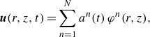 \begin{equation} \boldsymbol {u}(r,z,t) = \sum _{n=1}^{N} a^{n}(t)\,\varphi ^{n}(r,z), \end{equation}
where $N$
is the number of snapshots, and
$N$
is the number of snapshots, and $u$
represents the matrix of velocity fluctuations.
$u$
represents the matrix of velocity fluctuations.
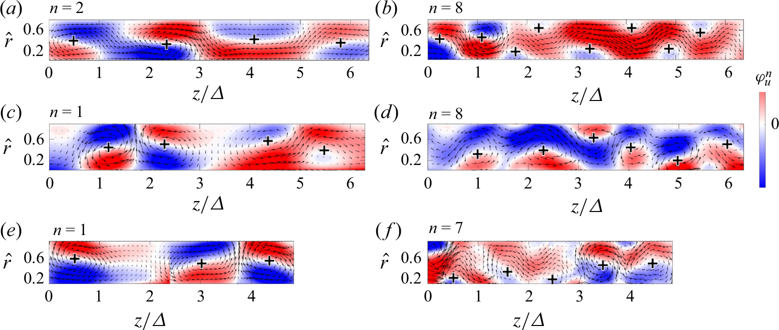
Figure 11. The POD modes with the largest Taylor vortices for $\varDelta /d$
values (a) 1/16, (c) 1/8 and (e) 1/4, alongside POD modes identifying Görtler vortices for
$\varDelta /d$
values (a) 1/16, (c) 1/8 and (e) 1/4, alongside POD modes identifying Görtler vortices for $\varDelta /d$
values (b) 1/16, (d) 1/8 and (f) 1/4. Here,
$\varDelta /d$
values (b) 1/16, (d) 1/8 and (f) 1/4. Here, $Re = 2 \times 10^3$
.
$Re = 2 \times 10^3$
.
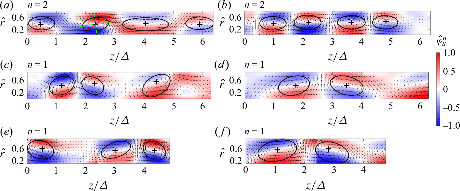
Figure 12. Comparison of the most dominant POD modes between $Re=2\times 10^3$
for
$Re=2\times 10^3$
for $\varDelta /d $
values (a) 1/16, (c) 1/8 and (e) 1/4, and
$\varDelta /d $
values (a) 1/16, (c) 1/8 and (e) 1/4, and $Re=10^4$
for
$Re=10^4$
for $\varDelta /d $
values (b) 1/16, (d) 1/8 and (f) 1/4. The elliptical regions highlight the identified core areas of Taylor cells in each case.
$\varDelta /d $
values (b) 1/16, (d) 1/8 and (f) 1/4. The elliptical regions highlight the identified core areas of Taylor cells in each case.
The normalised POD modes for $\varDelta /d=1/16$
, 1/8 and 1/4 at
$\varDelta /d=1/16$
, 1/8 and 1/4 at $Re = 2 \times 10^3$
are presented in figure 11, with superimposed velocity vectors to visualise vortical structures. The vortex core locations are marked by ‘
$Re = 2 \times 10^3$
are presented in figure 11, with superimposed velocity vectors to visualise vortical structures. The vortex core locations are marked by ‘ $+$
’ symbols. The first two POD modes successfully capture the dominant Taylor cells, as seen in figure 11(a,c,e), whereas weaker Görtler vortices appear only in the higher modes (figure 11
b,d,f). Note that POD is unable to isolate Görtler vortices because of the dominance of Taylor cells. A blend of Taylor and Görtler vortices is observed in the higher-order POD modes, highlighting their interaction. This interaction can be seen at
$+$
’ symbols. The first two POD modes successfully capture the dominant Taylor cells, as seen in figure 11(a,c,e), whereas weaker Görtler vortices appear only in the higher modes (figure 11
b,d,f). Note that POD is unable to isolate Görtler vortices because of the dominance of Taylor cells. A blend of Taylor and Görtler vortices is observed in the higher-order POD modes, highlighting their interaction. This interaction can be seen at $z/\varDelta = 1.7$
in figure 11(b),
$z/\varDelta = 1.7$
in figure 11(b), $z/\varDelta = 1$
and 5 in figure 11(d), and
$z/\varDelta = 1$
and 5 in figure 11(d), and $z/\varDelta = 0.5$
and 2.5 in figure 11(f). In these regions, Görtler vortices grow from the surface, breaking down a single large-scale Taylor cell into smaller cells, consistent with interactions shown in figures 8 and 9. For complementary insight, refer to the supplementary movies.
$z/\varDelta = 0.5$
and 2.5 in figure 11(f). In these regions, Görtler vortices grow from the surface, breaking down a single large-scale Taylor cell into smaller cells, consistent with interactions shown in figures 8 and 9. For complementary insight, refer to the supplementary movies.
Figure 12 illustrates the POD modes containing the largest Taylor cell for the lowest and highest $Re$
at different gap sizes, demonstrating the effect of these factors on the dominant Taylor cell dimension. Here, the vortex core areas are identified by their maximum tangential velocity magnitude (see figure 4). The normalised tangential velocity profiles along the major and minor axes of the POD modes in figure 13 further highlight the effects of gap size and
$Re$
at different gap sizes, demonstrating the effect of these factors on the dominant Taylor cell dimension. Here, the vortex core areas are identified by their maximum tangential velocity magnitude (see figure 4). The normalised tangential velocity profiles along the major and minor axes of the POD modes in figure 13 further highlight the effects of gap size and $Re$
. At low
$Re$
. At low $Re$
, figure 13(a) shows the longest major axis for the smallest gap. At higher
$Re$
, figure 13(a) shows the longest major axis for the smallest gap. At higher $Re$
, this trend reverses. Figure 13(c) shows that the major axis length increases with increasing gap size at
$Re$
, this trend reverses. Figure 13(c) shows that the major axis length increases with increasing gap size at $Re = 10^4$
. The minor axis length also increases with gap size for all
$Re = 10^4$
. The minor axis length also increases with gap size for all $Re$
values, though with less significant changes compared to the major axis (figure 13
b,d), indicating that radial expansion is limited mainly by the gap size.
$Re$
values, though with less significant changes compared to the major axis (figure 13
b,d), indicating that radial expansion is limited mainly by the gap size.
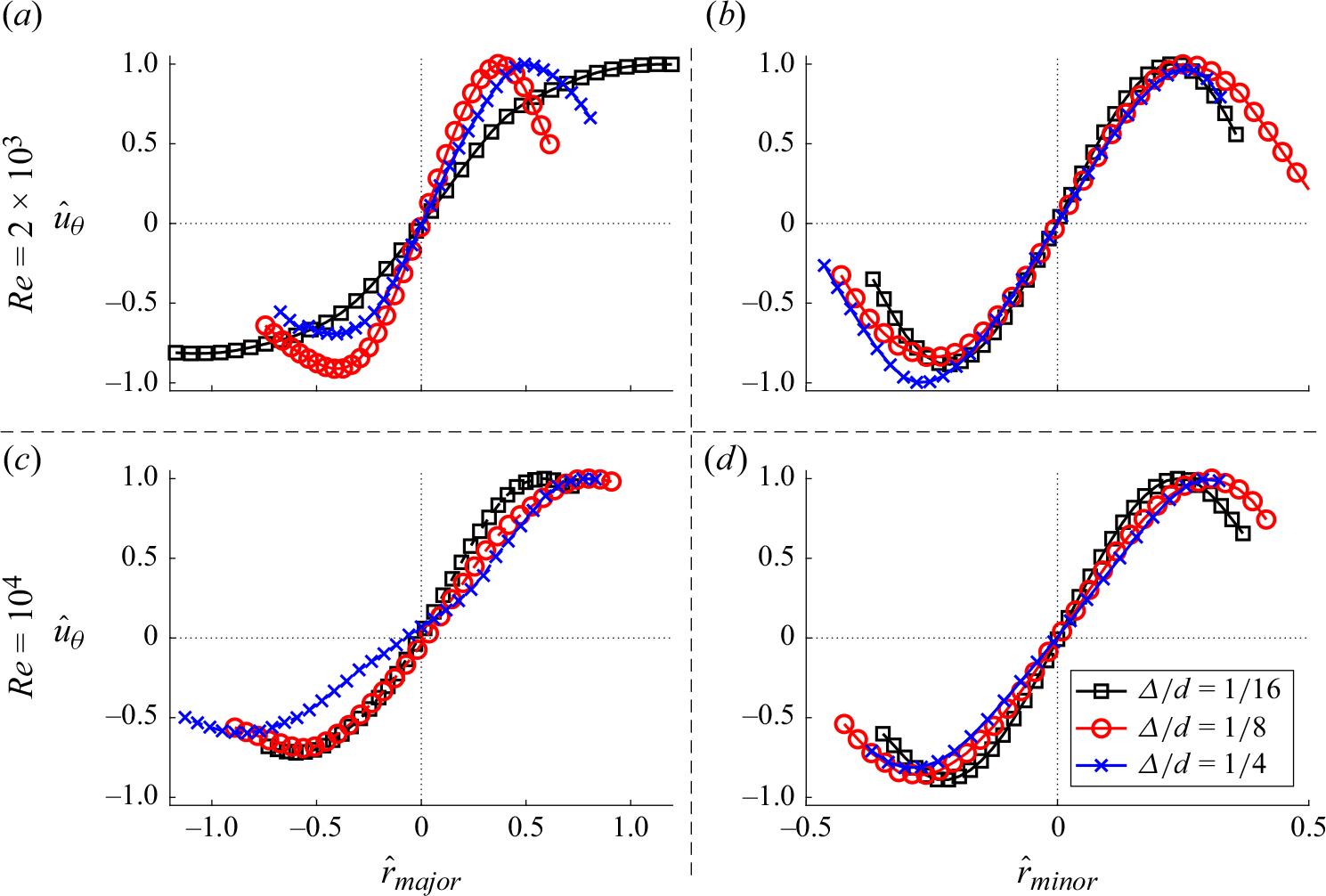
Figure 13. Profiles of tangential velocity for Taylor cells in the most dominant POD mode along the major and minor axes for $\varDelta /d =1/16$
, 1/8 and 1/4 at
$\varDelta /d =1/16$
, 1/8 and 1/4 at $Re = 2 \times 10^3$
and
$Re = 2 \times 10^3$
and $10^4$
.
$10^4$
.
While POD effectively identifies dominant energy structures, it faces limitations in distinguishing large-scale Taylor cells from smaller-scale Görtler vortices due to its lack of frequency and wavenumber resolution. As demonstrated in figures 11 and 12, the POD modes exhibit a combined structure that is predominantly influenced by Taylor cells, making it challenging to isolate and capture smaller-scale features such as Görtler vortices.
To address such limitations, we applied spectral POD (SPOD) to two selected cases, demonstrating how SPOD effectively captures both spatial and temporal coherence. Unlike traditional POD, SPOD integrates the benefits of dynamic mode decomposition (DMD) and space-only POD, enabling finer separation of coherent structures. This method retains the energy ranking and orthogonality features of POD-based approaches, as introduced by Lumley (Reference Lumley1970). By producing optimal, averaged DMD modes, SPOD offers a more detailed view of structure interactions across scales (Tu et al. Reference Tu, Rowley, Luchtenburg, Brunton and Kutz2014). The SPOD implementation follows the methodology by Sieber, Paschereit & Oberleithner (Reference Sieber, Paschereit and Oberleithner2016).
The first step of SPOD is to apply Welch’s method, which divides a single time series of $N_T$
snapshots into overlapping segments of
$N_T$
snapshots into overlapping segments of $N_{FFT}$
snapshots to capture statistical variability. Here,
$N_{FFT}$
snapshots to capture statistical variability. Here, $N_{FFT}$
is set to 512, providing frequency resolution 0.2 Hz. A discrete Fourier transform is applied to each segment
$N_{FFT}$
is set to 512, providing frequency resolution 0.2 Hz. A discrete Fourier transform is applied to each segment $q^k(T_j)$
, yielding the Fourier coefficient
$q^k(T_j)$
, yielding the Fourier coefficient $\hat {q}^k(f_m)$
:
$\hat {q}^k(f_m)$
:
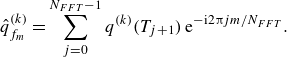 \begin{equation} \hat {q}^{(k)}_{f_{m}}=\sum _{j=0}^{N_{{FFT}}-1} q^{(k)}(T_{j+1})\,{\rm e}^{-{\rm i}2 \unicode{x03C0} j m / N_{{FFT}}}. \end{equation}
For each frequency $f_{m}$
, we construct
$f_{m}$
, we construct $\hat {Q}_{f_{m}}= [\hat {q}_{f_{m}}^{(1)} , \hat {q}_{f_{m}}^{(2)} , \ldots , \hat {q}_{f_{m}}^{(N_r)} ]$
,
$\hat {Q}_{f_{m}}= [\hat {q}_{f_{m}}^{(1)} , \hat {q}_{f_{m}}^{(2)} , \ldots , \hat {q}_{f_{m}}^{(N_r)} ]$
, $\hat {Q} \in \mathbb{C}^{M \times N_r}$
, where
$\hat {Q} \in \mathbb{C}^{M \times N_r}$
, where $M$
is the number of spatial points, and
$M$
is the number of spatial points, and $N_r$
is the number of realisations. Singular value decomposition is applied to
$N_r$
is the number of realisations. Singular value decomposition is applied to $\hat {Q}$
, as in traditional POD. For more SPOD details, see Schmidt & Colonius (Reference Schmidt and Colonius2020).
$\hat {Q}$
, as in traditional POD. For more SPOD details, see Schmidt & Colonius (Reference Schmidt and Colonius2020).
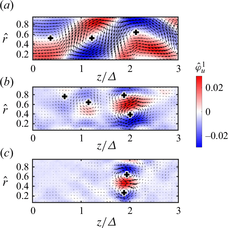
Figure 14. The first SPOD modes for $Re = 2 \times 10^3$
and
$Re = 2 \times 10^3$
and $\varDelta /d = 1/4$
at frequencies (a)
$\varDelta /d = 1/4$
at frequencies (a) $f = 0$
Hz, (b)
$f = 0$
Hz, (b) $f = 0.4$
Hz, and (c)
$f = 0.4$
Hz, and (c) $f = 0.6$
Hz.
$f = 0.6$
Hz.
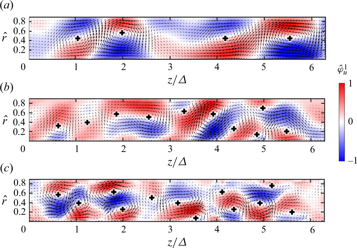
Figure 15. The first SPOD modes for $Re = 2\times 10^3$
and
$Re = 2\times 10^3$
and $\varDelta /d=1/8$
, for (a)
$\varDelta /d=1/8$
, for (a) $f = 0$
Hz, (b)
$f = 0$
Hz, (b) $f = 0.4$
Hz, and (c)
$f = 0.4$
Hz, and (c) $f = 0.6$
Hz.
$f = 0.6$
Hz.
The first SPOD modes for the two selected cases $\varDelta /d = 1/4$
and
$\varDelta /d = 1/4$
and $1/8$
at
$1/8$
at $Re = 2000$
are shown in figures 14 and 15, illustrating three mode frequencies:
$Re = 2000$
are shown in figures 14 and 15, illustrating three mode frequencies: $f = 0$
, 0.4 and 0.6 Hz. With the additional frequency information, SPOD effectively separates different scales of coherent structures. The zero-frequency mode captures the largest-scale Taylor vortices in both cases (figures 14(a) and 15(a)). However, differences appear in the higher-frequency modes. For the largest gap,
$f = 0$
, 0.4 and 0.6 Hz. With the additional frequency information, SPOD effectively separates different scales of coherent structures. The zero-frequency mode captures the largest-scale Taylor vortices in both cases (figures 14(a) and 15(a)). However, differences appear in the higher-frequency modes. For the largest gap, $\varDelta /d = 1/4$
(figure 14), higher-frequency modes reveal multiple Görtler vortices emerging near the wall with its vortex centre forming between the Taylor cells, whereas in the
$\varDelta /d = 1/4$
(figure 14), higher-frequency modes reveal multiple Görtler vortices emerging near the wall with its vortex centre forming between the Taylor cells, whereas in the $\varDelta /d = 1/8$
case (figure 15), the Görtler cells coexist with smaller Taylor vortices, evidencing the role of the gap size.
$\varDelta /d = 1/8$
case (figure 15), the Görtler cells coexist with smaller Taylor vortices, evidencing the role of the gap size.
The SPOD energy spectrum shown in figure 16 demonstrates a scaling behaviour across frequencies, indicating energy exchange between Taylor and Görtler vortices through the mechanism shown in figure 9. This mechanism is visualised in supplementary movie 2. For both cases, scaling extends from the lowest frequencies to a saturation frequency $f \approx 2$
Hz, aligning with the Kolmogorov inertial subrange, implying a cascade process. The larger gap case exhibits two scaling regimes:
$f \approx 2$
Hz, aligning with the Kolmogorov inertial subrange, implying a cascade process. The larger gap case exhibits two scaling regimes: $\beta \approx -5/3$
for the low-frequency range, and
$\beta \approx -5/3$
for the low-frequency range, and $\beta \approx -3$
for smaller structures. In contrast, the
$\beta \approx -3$
for smaller structures. In contrast, the $\varDelta /d=1/8$
case shows the latter scaling. The
$\varDelta /d=1/8$
case shows the latter scaling. The $-3$
scaling is likely related to the anisotropic energy transfer mechanism in rotating turbulence demonstrated in Zakharov, L’vov & Falkovich (Reference Zakharov, L’vov and Falkovich2012), and the difference in SPOD spectrum further highlights the influence of gap size on vortex dynamics and energy distribution.
$-3$
scaling is likely related to the anisotropic energy transfer mechanism in rotating turbulence demonstrated in Zakharov, L’vov & Falkovich (Reference Zakharov, L’vov and Falkovich2012), and the difference in SPOD spectrum further highlights the influence of gap size on vortex dynamics and energy distribution.
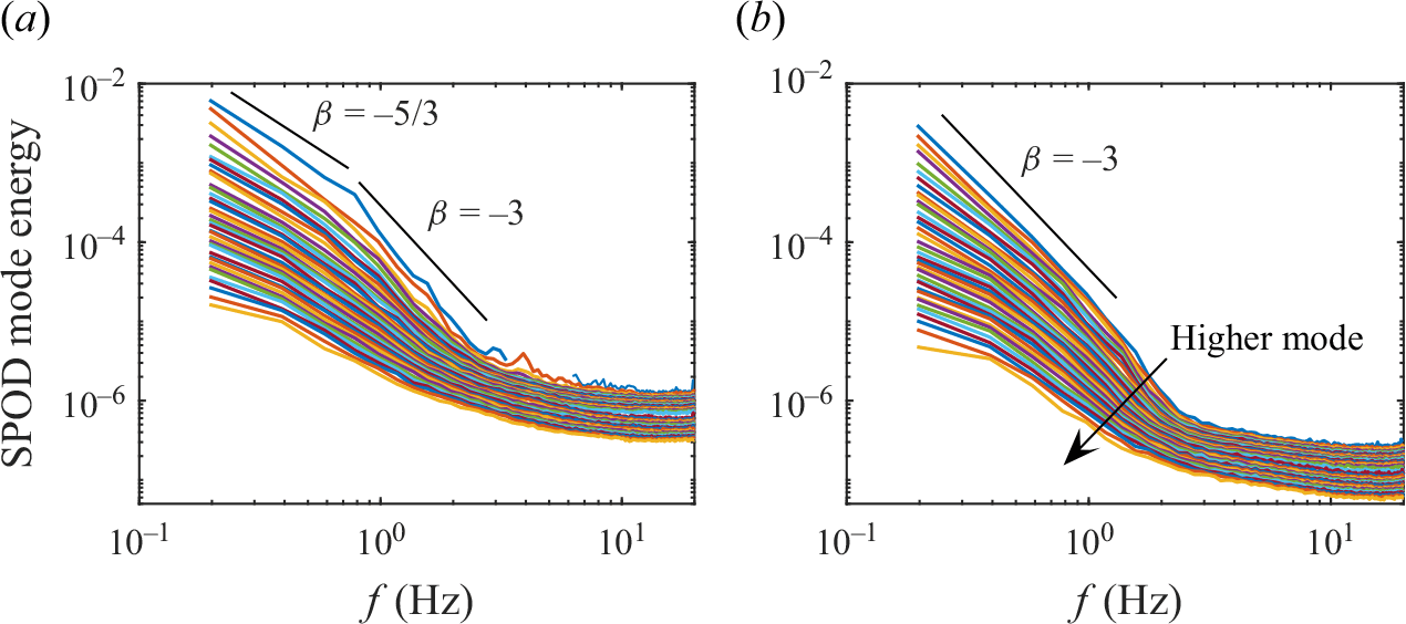
Figure 16. The SPOD energy spectrum for (a) $Re = 2\times 10^3$
and
$Re = 2\times 10^3$
and $\varDelta /d = 1/4$
, and (b)
$\varDelta /d = 1/4$
, and (b) $Re = 2\times 10^3$
and
$Re = 2\times 10^3$
and $\varDelta /d = 1/8$
.
$\varDelta /d = 1/8$
.
4. Discussion
This study provides new insights into the dynamics of TC flows within square enclosures, particularly regarding the influence of geometry and gap size on vortex evolution. Unlike circular TC systems, the square enclosure introduces additional constraints and flow interactions that alter the development and stability of vortices.
A key finding is the role of the square enclosure in modifying the mean velocity gradient, particularly near the corners, where Moffatt vortices are expected to develop. These vortices, interacting with Taylor and Görtler structures, could introduce additional complexity to the flow dynamics. However, confirming their exact influence requires further investigation.
A central challenge in characterising these flows is selecting an appropriate Reynolds number definition. While the conventional Reynolds number based on the inner cylinder radius $Re = \Omega r_0^2 / \nu$
is useful for comparing with classical TC studies, it does not account for variations in shear across the domain. Conversely, the shear-based Reynolds number
$Re = \Omega r_0^2 / \nu$
is useful for comparing with classical TC studies, it does not account for variations in shear across the domain. Conversely, the shear-based Reynolds number $Re_{\varDelta } = \Omega r_0 \varDelta / \nu$
captures the influence of the minimum gap. However, it does not incorporate the strong azimuthal variability of the mean shear gradient induced by the square enclosure. This variability results in alternating regions of favourable and adverse pressure gradients, affecting vortex stability and interactions in a manner not captured by either Reynolds number alone.
$Re_{\varDelta } = \Omega r_0 \varDelta / \nu$
captures the influence of the minimum gap. However, it does not incorporate the strong azimuthal variability of the mean shear gradient induced by the square enclosure. This variability results in alternating regions of favourable and adverse pressure gradients, affecting vortex stability and interactions in a manner not captured by either Reynolds number alone.
In the turbulence regime studied, a critical observation is the modulation of Taylor vortices by Görtler vortices, particularly in wider gaps. These interactions suggest a mechanism for energy transfer between scales, where Görtler vortices may bridge the gap between large-scale Taylor vortices and smaller-scale turbulent eddies. High-resolution simulations or targeted experiments could further elucidate this mechanism, and quantify its contribution to energy redistribution.
The study also shows the significance of radial outflow boundaries in shaping vortex interactions. The interaction of radial flows with the square enclosure leads to periodic vortex formation and decay, a behaviour less pronounced in circular geometries. This phenomenon has practical implications for applications requiring controlled turbulence, such as mixing and transport systems. The modulation of Taylor and Görtler vortices by the square geometry presents opportunities for flow manipulation, which could be explored further in polygonal enclosures with different aspect ratios.
The linear stability analysis presented in Appendix B provides additional context for the observed flow behaviour. The primary instability remains a Taylor vortex mode similar to that in circular enclosures, but lower-growth-rate corner modes emerge due to the square geometry. These modes, influenced by the separation regions at the enclosure’s corners, may interact with other instability mechanisms and contribute to a bypass transition to turbulence (Schmid & Henningson Reference Schmid and Henningson2001). The variation in cross-sectional area across the square geometry introduces pressure gradients that alternate between favourable and adverse regions, affecting flow stability. The critical Reynolds number ( $Re_c$
) for the square enclosure is lower than that for a circular system. For example, at radius ratio 0.5, the circular case has critical Reynolds number
$Re_c$
) for the square enclosure is lower than that for a circular system. For example, at radius ratio 0.5, the circular case has critical Reynolds number $Re_c=68.19$
with axial wavenumber
$Re_c=68.19$
with axial wavenumber $\alpha _c = 3.16$
(Fasel & Booz Reference Fasel and Booz1984), whereas the square system yields a lower
$\alpha _c = 3.16$
(Fasel & Booz Reference Fasel and Booz1984), whereas the square system yields a lower $Re_c=56.7$
at
$Re_c=56.7$
at $\alpha _c = 2.62$
.
$\alpha _c = 2.62$
.
Before the onset of fully developed turbulence, the flow undergoes successive bifurcations. Higher-order instabilities, such as wavy Taylor vortices, are observed in narrow-gap TC systems ( $d/(d + \varDelta ) \gt 0.75$
). Although the present stability analysis (Appendix B) focuses primarily on the first instability modes, the presence of secondary bifurcations suggests a structured transition to turbulence. In circular TC flows, azimuthal disturbances influence these transitions, while in square enclosures, the discrete symmetry imposes constraints on their development. Further work is required to characterise the role of these intermediate flow states and their impact on the transition process.
$d/(d + \varDelta ) \gt 0.75$
). Although the present stability analysis (Appendix B) focuses primarily on the first instability modes, the presence of secondary bifurcations suggests a structured transition to turbulence. In circular TC flows, azimuthal disturbances influence these transitions, while in square enclosures, the discrete symmetry imposes constraints on their development. Further work is required to characterise the role of these intermediate flow states and their impact on the transition process.
The findings presented here highlight the complex interplay between geometry, instability mechanisms and turbulence dynamics in square TC systems. Future work should focus on extending experimental and computational efforts to capture finer details of vortex interactions, particularly in the presence of dynamically evolving Görtler structures. Investigating alternative polygonal enclosures, such as hexagonal or octagonal cross-sections, may offer further insights into the role of boundary constraints on vortex evolution. Also, real-time flow control strategies could be explored to manipulate vortex interactions and modulate the transition to turbulence, opening new avenues for flow engineering applications.
5. Conclusions
We explored the dynamics of Taylor–Couette (TC) flows within square enclosures, focusing primarily on the characteristics of dominant turbulent motions and the effects of varying gap sizes and Reynolds numbers on vortex formation and flow patterns.
Vortex formation and dynamics were examined using various identification methods and modal analysis techniques, including POD and SPOD. Vortices with opposite rotations tended to strengthen and elongate each other, often leading to break-up, while vortices with the same rotation generally merged, although some dissipated due to nearby influences. The interactions between vortical structures are confirmed by the SPOD spectrum, which exhibits scaling within the frequency range $f = 0{-}2$
Hz, indicating the presence of a cascade process. The space–time evolution of radial velocity at
$f = 0{-}2$
Hz, indicating the presence of a cascade process. The space–time evolution of radial velocity at $\hat {r}=0.5$
highlighted the persistence and variability of Taylor vortices, with larger gaps and lower Reynolds numbers exhibiting more persistent structures, whereas higher Reynolds numbers and smaller gaps displayed increased turbulence and irregular motions. The compensated spectra of the axial velocity component revealed distinct flow dynamics. At
$\hat {r}=0.5$
highlighted the persistence and variability of Taylor vortices, with larger gaps and lower Reynolds numbers exhibiting more persistent structures, whereas higher Reynolds numbers and smaller gaps displayed increased turbulence and irregular motions. The compensated spectra of the axial velocity component revealed distinct flow dynamics. At $Re = 2\times 10^3$
, the energy distribution indicated a nearly laminar flow, whereas higher Reynolds numbers showed a broadband energy distribution with increased energy across all measured scales. A consistent shift of the compensated spectral peak to higher frequencies with increasing Reynolds number was observed across all gap sizes. The study also highlights the role of Görtler vortices in forming new Taylor cells, particularly in the presence of radial outflow boundaries. These interactions led to the formation of smaller-scale vortices, indicating a complex interplay of vortex structures within the flow.
$Re = 2\times 10^3$
, the energy distribution indicated a nearly laminar flow, whereas higher Reynolds numbers showed a broadband energy distribution with increased energy across all measured scales. A consistent shift of the compensated spectral peak to higher frequencies with increasing Reynolds number was observed across all gap sizes. The study also highlights the role of Görtler vortices in forming new Taylor cells, particularly in the presence of radial outflow boundaries. These interactions led to the formation of smaller-scale vortices, indicating a complex interplay of vortex structures within the flow.
The POD mode shapes are used to characterise how variations in $Re$
and gap size influence the largest Taylor vortices, highlighting that the radial expansion of these vortices is constrained primarily by the gap size. It is worth highlighting the role of
$Re$
and gap size influence the largest Taylor vortices, highlighting that the radial expansion of these vortices is constrained primarily by the gap size. It is worth highlighting the role of $Re$
and gap size in the spectral distribution of velocity fluctuations. For a given
$Re$
and gap size in the spectral distribution of velocity fluctuations. For a given $Re$
, the energy distribution of larger motions exhibited a similar pattern across varying gaps. However, there was a monotonic increase in energy at higher frequencies beyond the integral-type frequency
$Re$
, the energy distribution of larger motions exhibited a similar pattern across varying gaps. However, there was a monotonic increase in energy at higher frequencies beyond the integral-type frequency $f_I$
. The reduced form of this frequency,
$f_I$
. The reduced form of this frequency, $f\varDelta /\Omega _i r_i$
, was approximately 1/10. SPOD further revealed the impact of gap size on the spectral scaling regimes, with the larger gap size displaying two distinct scaling behaviours, while the smaller gap size exhibited a single scaling regime.
$f\varDelta /\Omega _i r_i$
, was approximately 1/10. SPOD further revealed the impact of gap size on the spectral scaling regimes, with the larger gap size displaying two distinct scaling behaviours, while the smaller gap size exhibited a single scaling regime.
Finally, the linear stability analysis described in Appendix B identified the primary instability mechanism linked to interactions between Taylor vortices. Eigenvalue spectra for different gap sizes highlighted the critical Reynolds numbers and wavenumbers where instability occurs, providing insights into the initial vortex onset. Laboratory experiments, conducted over Reynolds numbers ranging from $2\times 10^3$
to
$2\times 10^3$
to $10^4$
, and gap sizes
$10^4$
, and gap sizes $\varDelta /d=1/16$
, 1/8 and 1/4, revealed that lower Reynolds numbers exhibited well-defined Taylor vortices. As the Reynolds number increased, the flow transitioned to a turbulent state characterised by multi-scale vortices. The interactions between Taylor and Görtler vortices significantly influenced the flow dynamics, especially at higher Reynolds numbers.
$\varDelta /d=1/16$
, 1/8 and 1/4, revealed that lower Reynolds numbers exhibited well-defined Taylor vortices. As the Reynolds number increased, the flow transitioned to a turbulent state characterised by multi-scale vortices. The interactions between Taylor and Görtler vortices significantly influenced the flow dynamics, especially at higher Reynolds numbers.
Supplementary movies
Supplementary movies are available at https://doi.org/10.1017/jfm.2025.10251.
Acknowledgement
V.N. expresses his gratitude to the United States India Education Foundation (USIEF) for the Fulbright–Nehru fellowship, which enabled his participation in the study.
Declaration of interests
The authors report no conflict of interest.
Appendix A. Comparison of selected cases sharing $\boldsymbol{Re}_{\boldsymbol{\varDelta }}$

In classical TC flow, the gap between concentric cylinders serves as a natural length scale over which shear develops. However, in the present configuration with a square outer cylinder, this length scale is not well defined, as the gap $\varDelta$
varies with the angular position
$\varDelta$
varies with the angular position $\theta$
, as shown in figure 17. This variation imposes continuous changes in the mean shear gradient, with alternating regions of favourable and adverse pressure gradients. Consequently, selecting a single characteristic gap length – whether the minimum, maximum, or an average – is insufficient to fully capture the flow dynamics. To illustrate this, we compare selected cases that share the Reynolds number based on the minimum gap,
$\theta$
, as shown in figure 17. This variation imposes continuous changes in the mean shear gradient, with alternating regions of favourable and adverse pressure gradients. Consequently, selecting a single characteristic gap length – whether the minimum, maximum, or an average – is insufficient to fully capture the flow dynamics. To illustrate this, we compare selected cases that share the Reynolds number based on the minimum gap, $Re_{\varDelta }$
.
$Re_{\varDelta }$
.
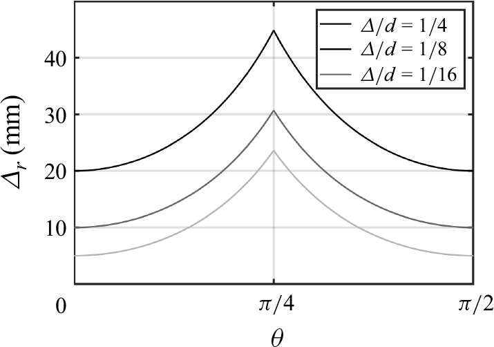
Figure 17. Variation of the (radial) gap over a quarter of the domain as a function of $\theta$
, where
$\theta$
, where $\theta = 0$
corresponds to the minimum gap.
$\theta = 0$
corresponds to the minimum gap.
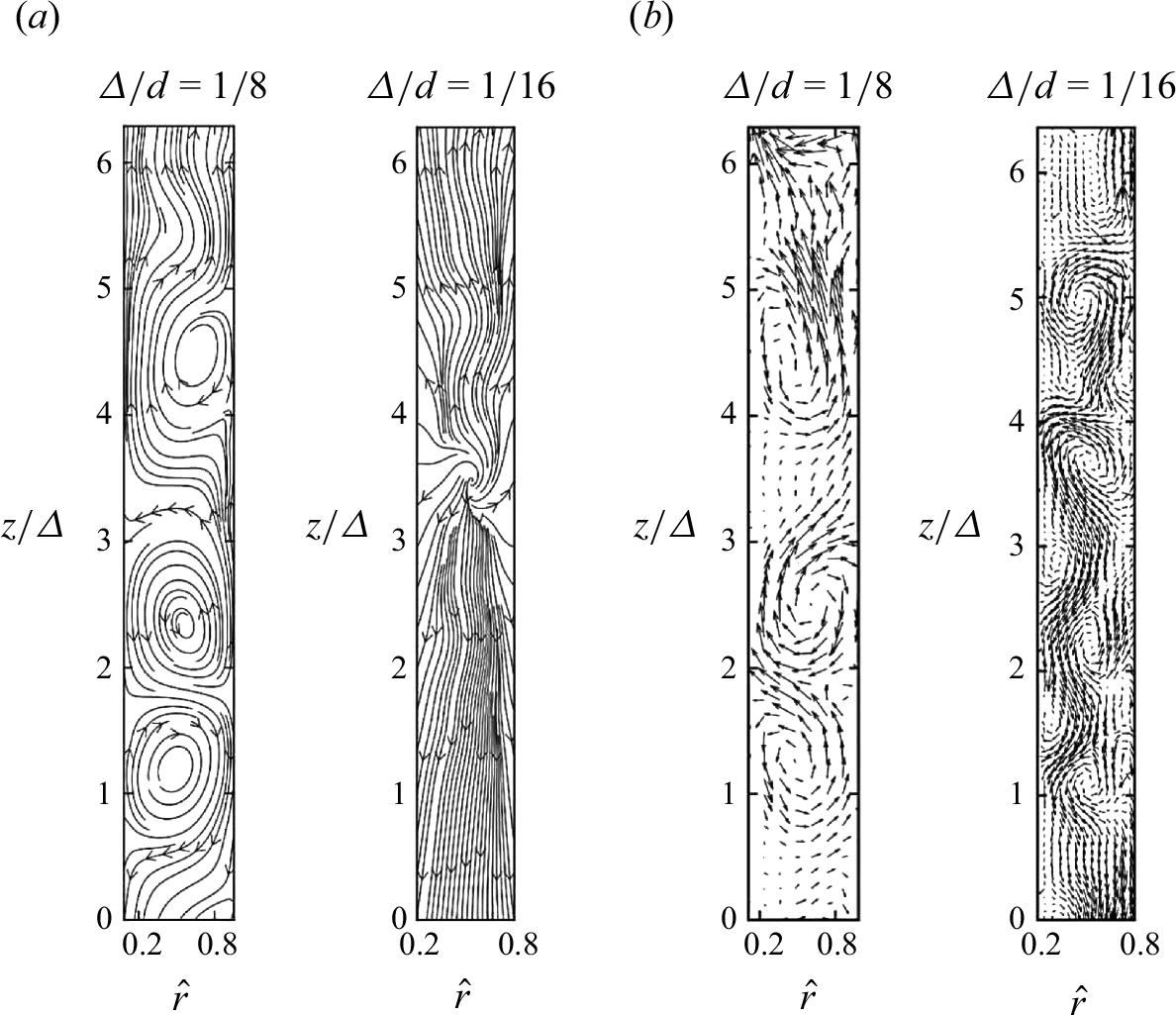
Figure 18. (a) Streamlines and (b) instantaneous velocity vectors at shared $Re_{\varDelta } \approx 460$
for the
$Re_{\varDelta } \approx 460$
for the $\varDelta /d=1/8$
and 1/16 systems.
$\varDelta /d=1/8$
and 1/16 systems.
Among the cases examined, a shear Reynolds number $Re_{\varDelta } \approx 460$
is shared between
$Re_{\varDelta } \approx 460$
is shared between $\varDelta /d = 1/16$
and
$\varDelta /d = 1/16$
and $\varDelta /d = 1/8$
. The mean velocity profiles in figure 18(a) show a well-defined Taylor cell structure for
$\varDelta /d = 1/8$
. The mean velocity profiles in figure 18(a) show a well-defined Taylor cell structure for $\varDelta /d = 1/8$
, whereas the velocity profile for
$\varDelta /d = 1/8$
, whereas the velocity profile for $\varDelta /d = 1/16$
appears irregular. The instantaneous velocity fields in figure 18(b) confirm the presence of Taylor cell structures in both cases, though they exhibit irregular temporal behaviour in the
$\varDelta /d = 1/16$
appears irregular. The instantaneous velocity fields in figure 18(b) confirm the presence of Taylor cell structures in both cases, though they exhibit irregular temporal behaviour in the $\varDelta /d = 1/16$
case, leading to their absence in the time-averaged velocity field.
$\varDelta /d = 1/16$
case, leading to their absence in the time-averaged velocity field.
Further insight is provided in figure 17, which shows that the ratio of maximum to minimum gap width is approximately 4.72 for $\varDelta /d = 1/16$
, 3.07 for
$\varDelta /d = 1/16$
, 3.07 for $\varDelta /d = 1/8$
, and 2.24 for
$\varDelta /d = 1/8$
, and 2.24 for $\varDelta /d = 1/4$
. This trend suggests that as the gap narrows, the flow experiences stronger adverse pressure gradients. At sufficiently small gap ratios, these pressure effects may outweigh centrifugal instabilities, suppressing coherent Taylor cell formation. Identifying a critical gap ratio beyond which adverse pressure gradients dominate centrifugal effects would be an important avenue for future research. Also, investigating the temporal dynamics of the irregular motion at
$\varDelta /d = 1/4$
. This trend suggests that as the gap narrows, the flow experiences stronger adverse pressure gradients. At sufficiently small gap ratios, these pressure effects may outweigh centrifugal instabilities, suppressing coherent Taylor cell formation. Identifying a critical gap ratio beyond which adverse pressure gradients dominate centrifugal effects would be an important avenue for future research. Also, investigating the temporal dynamics of the irregular motion at $\varDelta /d = 1/16$
could provide further insight into the mechanisms governing Taylor cell breakdown in highly confined flows.
$\varDelta /d = 1/16$
could provide further insight into the mechanisms governing Taylor cell breakdown in highly confined flows.
Another shear Reynolds number, $Re_{\varDelta } = 917$
, shared among
$Re_{\varDelta } = 917$
, shared among $ \varDelta /d = 1/16$
,
$ \varDelta /d = 1/16$
, $1/8$
and
$1/8$
and $1/4$
, exhibits similar trends. The mean and instantaneous velocity profiles for these cases, shown in figure 19, align with observations from the lower
$1/4$
, exhibits similar trends. The mean and instantaneous velocity profiles for these cases, shown in figure 19, align with observations from the lower $Re_{\varDelta }$
case. While Taylor cells are clearly present in the instantaneous velocity fields, their absence in the mean velocity profile for
$Re_{\varDelta }$
case. While Taylor cells are clearly present in the instantaneous velocity fields, their absence in the mean velocity profile for $ \varDelta /d = 1/16$
suggests that adverse pressure gradients may be disrupting their long-term stability.
$ \varDelta /d = 1/16$
suggests that adverse pressure gradients may be disrupting their long-term stability.
Unlike the lower $Re_{\varDelta }$
case, the Taylor cell size, when non-dimensionalised by the minimum gap, remains comparable in the mean velocity profiles for
$Re_{\varDelta }$
case, the Taylor cell size, when non-dimensionalised by the minimum gap, remains comparable in the mean velocity profiles for $ \varDelta /d = 1/4$
and
$ \varDelta /d = 1/4$
and $1/8$
. Finally, the dominant vortex motion, as illustrated in figure 20(a), highlights the distinct influence of the gap size
$1/8$
. Finally, the dominant vortex motion, as illustrated in figure 20(a), highlights the distinct influence of the gap size $\varDelta$
at given
$\varDelta$
at given $Re_{\varDelta }$
.
$Re_{\varDelta }$
.

Figure 19. (a) Streamlines and (b) instantaneous velocity vectors at shared $Re_{\varDelta } \approx 920$
for the
$Re_{\varDelta } \approx 920$
for the $\varDelta /d=1/4$
, 1/8 and 1/16 systems.
$\varDelta /d=1/4$
, 1/8 and 1/16 systems.
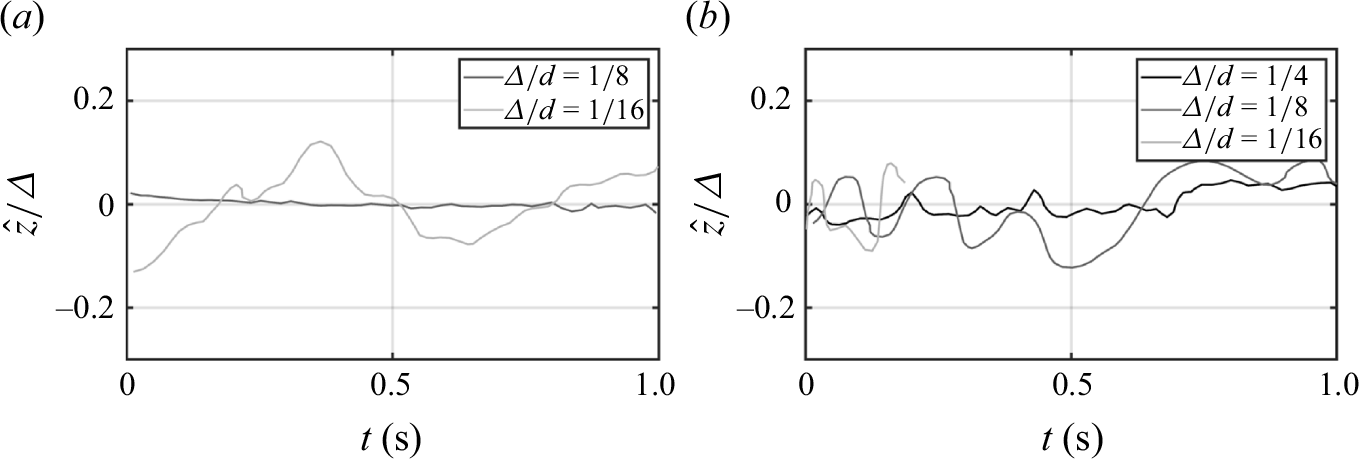
Figure 20. Vertical motions of a dominant vortex for (a) $Re_{\varDelta } \approx 460$
and (b)
$Re_{\varDelta } \approx 460$
and (b) $Re_{\varDelta } \approx 920$
for different
$Re_{\varDelta } \approx 920$
for different $\varDelta /d$
.
$\varDelta /d$
.
Appendix B. Linear stability analysis
Here, we explore the unstable modes in the linear transition regime of the flow. A meshless approach (Shahane et al. Reference Shahane, Radhakrishnan and Vanka2021) is used to compute the two-dimensional base flow, which is then analysed using global linear stability methods (Unnikrishnan et al. Reference Unnikrishnan, Narayanan and Vanka2024b ).
Let the field variables be of the form $\boldsymbol{q} = \boldsymbol{Q} + \boldsymbol{q}'$
, where
$\boldsymbol{q} = \boldsymbol{Q} + \boldsymbol{q}'$
, where $\boldsymbol{Q} = [U,V,W,P]^{\rm T}$
represents the base flow field,
$\boldsymbol{Q} = [U,V,W,P]^{\rm T}$
represents the base flow field, $\boldsymbol{q} = [u, v, w, p]^{\rm T}$
represents the instantaneous counterpart, and
$\boldsymbol{q} = [u, v, w, p]^{\rm T}$
represents the instantaneous counterpart, and $\boldsymbol{q}' = [u', v', w', p']^{\rm }T$
represents the perturbations. Subtracting the mean continuity and momentum equations from their instantaneous counterparts, and linearising them, provides the basis for the linear stability equations, written in Cartesian coordinates as follows:
$\boldsymbol{q}' = [u', v', w', p']^{\rm }T$
represents the perturbations. Subtracting the mean continuity and momentum equations from their instantaneous counterparts, and linearising them, provides the basis for the linear stability equations, written in Cartesian coordinates as follows:
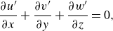 \begin{align}&\qquad\qquad\qquad\qquad\qquad\qquad \frac {\partial u'}{\partial x}+\frac {\partial v'}{\partial y}+\frac {\partial w'}{\partial z} = 0, \end{align}
 \begin{align}& \frac {\partial u'}{\partial t} + u'\frac {\partial U}{\partial x} + U\frac {\partial u'}{\partial x} + v'\frac {\partial U}{\partial y} + V\frac {\partial u'}{\partial y} + w'\frac {\partial U}{\partial z} = -\frac {\partial p'}{\partial x} + \frac {1}{Re}\left (\frac {\partial ^2 u'}{\partial x^2} + \frac {\partial ^2 u'}{\partial y^2} + \frac {\partial ^2 u'}{\partial z^2}\right )\!, \end{align}
 \begin{align}& \frac {\partial v'}{\partial t} + u'\frac {\partial V}{\partial x} + U\frac {\partial v'}{\partial x} + v'\frac {\partial V}{\partial y} + V\frac {\partial v'}{\partial y} + w'\frac {\partial V}{\partial z} = -\frac {\partial p'}{\partial y} + \frac {1}{Re}\left (\frac {\partial ^2 v'}{\partial x^2} + \frac {\partial ^2 v'}{\partial y^2} + \frac {\partial ^2 v'}{\partial z^2}\right ), \end{align}
 \begin{align}&\qquad\qquad \frac {\partial w'}{\partial t} + U\frac {\partial w'}{\partial x} + V\frac {\partial w'}{\partial y} = -\frac {\partial p'}{\partial z} + \frac {1}{Re}\left (\frac {\partial ^2 w'}{\partial x^2} + \frac {\partial ^2 w'}{\partial y^2} + \frac {\partial ^2 w'}{\partial z^2}\right ). \end{align}
Here, $(u,v,w)$
corresponds to the
$(u,v,w)$
corresponds to the $(x,y,z)$
coordinates (figure 2). We also use
$(x,y,z)$
coordinates (figure 2). We also use $(u_{r},u_{\theta },u_z)$
corresponding to the
$(u_{r},u_{\theta },u_z)$
corresponding to the $(r,\theta ,z)$
coordinates. A normal mode analysis is performed, assuming perturbations of the form
$(r,\theta ,z)$
coordinates. A normal mode analysis is performed, assuming perturbations of the form
 \begin{align} \boldsymbol{q}' = \hat {\boldsymbol{q}}(x,y) \exp {{\rm i} (\alpha z - \omega t)}, \end{align}
where $\alpha$
is the wavenumber, and
$\alpha$
is the wavenumber, and $\omega$
is a complex number,
$\omega$
is a complex number, $\omega _r + {\rm i} \omega _i$
. The real part (
$\omega _r + {\rm i} \omega _i$
. The real part ( $\omega _r$
) represents the frequency of the wave, and the imaginary part (
$\omega _r$
) represents the frequency of the wave, and the imaginary part ( $\omega _i$
) represents the temporal growth rate. The hat symbol indicates the Fourier amplitude of the normal mode corresponding to each of the field variables. The velocity components
$\omega _i$
) represents the temporal growth rate. The hat symbol indicates the Fourier amplitude of the normal mode corresponding to each of the field variables. The velocity components $U$
and
$U$
and $V$
are computed using the meshless method with a semi-implicit algorithm (Unnikrishnan et al. Reference Unnikrishnan, Shahane, Narayanan and Vanka2022). The axial velocity component of the base flow (
$V$
are computed using the meshless method with a semi-implicit algorithm (Unnikrishnan et al. Reference Unnikrishnan, Shahane, Narayanan and Vanka2022). The axial velocity component of the base flow ( $W$
) is zero. Also, the gradients of base velocity in the axial direction,
$W$
) is zero. Also, the gradients of base velocity in the axial direction, $\partial U/\partial z,\ \partial V/\partial z$
, are also zero. Substituting the normal mode form into the equations, we obtain
$\partial U/\partial z,\ \partial V/\partial z$
, are also zero. Substituting the normal mode form into the equations, we obtain
 \begin{align}& {\rm i} {\omega } \hat {u} = {\rm D}_x \hat {p} + (\mathcal{L} + {\rm D}_x U) \hat {u} + ({\rm D}_y U) \hat {v}, \\[-12pt]\nonumber \end{align}
 \begin{align}& {\rm i} {\omega } \hat {v} = {\rm D}_y \hat {p} + ({\rm D}_x V) \hat {u} + (\mathcal{L} + {\rm D}_y V) \hat {v}, \\[-12pt]\nonumber \end{align}
 \begin{align}&\qquad\qquad\,\, {\rm i} {\omega } \tilde {w} = \alpha \hat {p} + \mathcal{L} \tilde {w}, \\[-12pt]\nonumber \end{align}
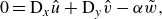 \begin{align}&\qquad\quad\, 0 = {\rm D}_x \hat {u} + {\rm D}_y \hat {v} - \alpha \tilde {w}, \end{align}
where $\mathcal{L} \equiv (U {\rm D}_x + V {\rm D}_y ) - ({1}/{Re}) ({\rm D}_x^2 + {\rm D}_y^2 - \alpha ^2 )$
,
$\mathcal{L} \equiv (U {\rm D}_x + V {\rm D}_y ) - ({1}/{Re}) ({\rm D}_x^2 + {\rm D}_y^2 - \alpha ^2 )$
, $\tilde {w} = {\rm i} \hat {w}$
, and
$\tilde {w} = {\rm i} \hat {w}$
, and ${\rm D}$
denotes the derivative in the directions mentioned by the subscript.
${\rm D}$
denotes the derivative in the directions mentioned by the subscript.
This linear system of equations can be written in matrix-vector form as
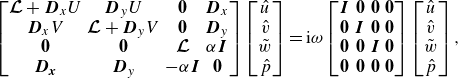 \begin{align}& \begin{bmatrix} \boldsymbol{\mathcal{L}}+\boldsymbol{D}_xU & \boldsymbol{D}_yU & \boldsymbol{0} & \boldsymbol{D}_x \\ \boldsymbol{D}_xV & \boldsymbol{\mathcal{L}}+\boldsymbol{D}_yV & \boldsymbol{0} & \boldsymbol{D}_y \\ \boldsymbol{0} & \boldsymbol{0} & \boldsymbol{\mathcal{L}} & \alpha \boldsymbol{I} \\ \boldsymbol{D_x} & \boldsymbol{D}_y & -\alpha \boldsymbol{I} & \boldsymbol{0} \end{bmatrix} \begin{bmatrix} \hat {u} \\ \hat {v} \\ \tilde {w} \\ \hat {p} \end{bmatrix} = {\rm i} \omega \begin{bmatrix} \boldsymbol{I} & \boldsymbol{0} & \boldsymbol{0} & \boldsymbol{0} \\ \boldsymbol{0} & \boldsymbol{I} & \boldsymbol{0} & \boldsymbol{0} \\ \boldsymbol{0} & \boldsymbol{0} & \boldsymbol{I} & \boldsymbol{0} \\ \boldsymbol{0} & \boldsymbol{0} & \boldsymbol{0} & \boldsymbol{0} \end{bmatrix} \begin{bmatrix} \hat {u} \\ \hat {v} \\ \tilde {w} \\ \hat {p} \end{bmatrix}, \end{align}
 \begin{align}&\qquad\qquad\qquad\qquad\qquad\qquad\quad \boldsymbol {A}\hat{\boldsymbol{q}} = {\rm i} \omega \boldsymbol {B}\hat{\boldsymbol{q}}, \end{align}
where A and B are linear operators on $\hat{\boldsymbol{q}}$
, and
$\hat{\boldsymbol{q}}$
, and ${\rm i} \omega$
is the eigenvalue corresponding to the eigenvector
${\rm i} \omega$
is the eigenvalue corresponding to the eigenvector $\hat{\boldsymbol{q}} = [\hat {u}, \hat {v}, \tilde {w}, \hat {p}]^{\rm T}$
.
$\hat{\boldsymbol{q}} = [\hat {u}, \hat {v}, \tilde {w}, \hat {p}]^{\rm T}$
.
Impermeability and no-slip conditions are used at the walls ( $u=v=w=0$
). These boundary conditions are imposed by adjusting the coefficients of the
$u=v=w=0$
). These boundary conditions are imposed by adjusting the coefficients of the $\boldsymbol{A}$
and
$\boldsymbol{A}$
and $\boldsymbol{B}$
matrices corresponding to the boundary points. Compatibility equations derived from linearised Navier–Stokes equations are collocated at the wall (Theofilis Reference Theofilis2003). These conditions are given by
$\boldsymbol{B}$
matrices corresponding to the boundary points. Compatibility equations derived from linearised Navier–Stokes equations are collocated at the wall (Theofilis Reference Theofilis2003). These conditions are given by
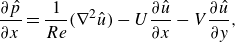 \begin{align}& \frac {\partial \hat {p}}{\partial x} = \frac {1}{Re}(\nabla ^2 \hat {u}) - U \frac {\partial \hat {u}}{\partial x} - V \frac {\partial \hat {u}}{\partial y}, \end{align}
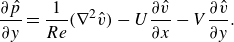 \begin{align}& \frac {\partial \hat {p}}{\partial y} = \frac {1}{Re}(\nabla ^2 \hat {v}) - U \frac {\partial \hat {v}}{\partial x} - V \frac {\partial \hat {v}}{\partial y}. \end{align}
The governing equations are invariant under complex conjugation, so only positive values of $\alpha$
need to be investigated. Here, we focus on the temporal growth, i.e.
$\alpha$
need to be investigated. Here, we focus on the temporal growth, i.e. $\alpha$
is a real number. The problem is also invariant to axial reflection, resulting in pairs of eigenvalues symmetric about the imaginary axis. The temporal modes
$\alpha$
is a real number. The problem is also invariant to axial reflection, resulting in pairs of eigenvalues symmetric about the imaginary axis. The temporal modes $\omega$
are sought for given
$\omega$
are sought for given $(\alpha , Re, \varDelta /d)$
, where
$(\alpha , Re, \varDelta /d)$
, where $\varDelta$
is the minimum radial gap between cylinders, and
$\varDelta$
is the minimum radial gap between cylinders, and $d$
is the diameter of the inner cylinder. This requires varying the parameters
$d$
is the diameter of the inner cylinder. This requires varying the parameters $(\alpha , Re)$
in an
$(\alpha , Re)$
in an $\mathcal{R}^2$
space for a given
$\mathcal{R}^2$
space for a given $\varDelta /d$
, with separate solutions of the eigenvalue problem for each case.
$\varDelta /d$
, with separate solutions of the eigenvalue problem for each case.
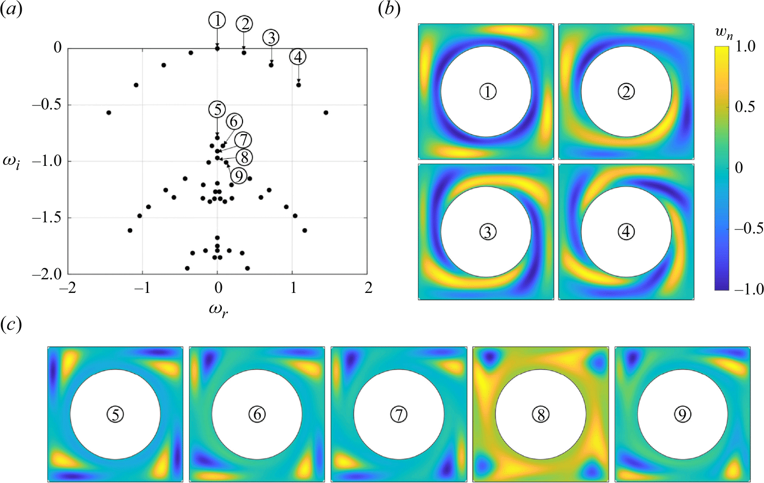
Figure 21. First modes at the critical Reynolds number $Re_c=116.4$
and critical wavenumber
$Re_c=116.4$
and critical wavenumber $\alpha =4.82$
for
$\alpha =4.82$
for $\varDelta /d=1/4$
mm. (a) Eigenvalue spectrum of complex frequencies
$\varDelta /d=1/4$
mm. (a) Eigenvalue spectrum of complex frequencies $\omega = \omega _r + {\rm i} \omega _i$
, with the imaginary axis corresponding to the growth rate of the mode, and the real axis representing frequency. (b) Eigenmodes governed by the cylinder rotation represented with contours of normalised axial velocity. (c) Corner modes governed by the secondary flow (separation region) at the corners of the square outer cylinder.
$\omega = \omega _r + {\rm i} \omega _i$
, with the imaginary axis corresponding to the growth rate of the mode, and the real axis representing frequency. (b) Eigenmodes governed by the cylinder rotation represented with contours of normalised axial velocity. (c) Corner modes governed by the secondary flow (separation region) at the corners of the square outer cylinder.
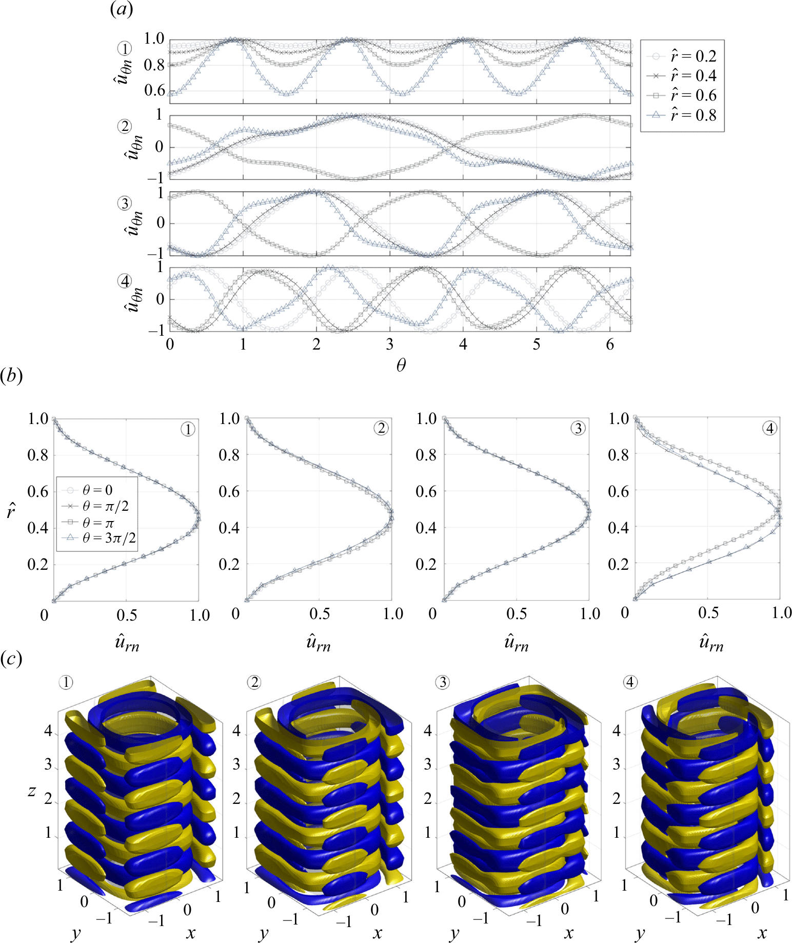
Figure 22. (a) Normalised tangential velocity $\hat {u}_{\theta n}$
at multiple radial locations. (b) Radial velocity
$\hat {u}_{\theta n}$
at multiple radial locations. (b) Radial velocity $\hat {u}_{r n}$
at multiple angular locations. (c) Isosurfaces of axial velocity at
$\hat {u}_{r n}$
at multiple angular locations. (c) Isosurfaces of axial velocity at $w_n = \pm 0.2$
, at the critical Reynolds number for
$w_n = \pm 0.2$
, at the critical Reynolds number for $\varDelta /d=1/4$
.
$\varDelta /d=1/4$
.
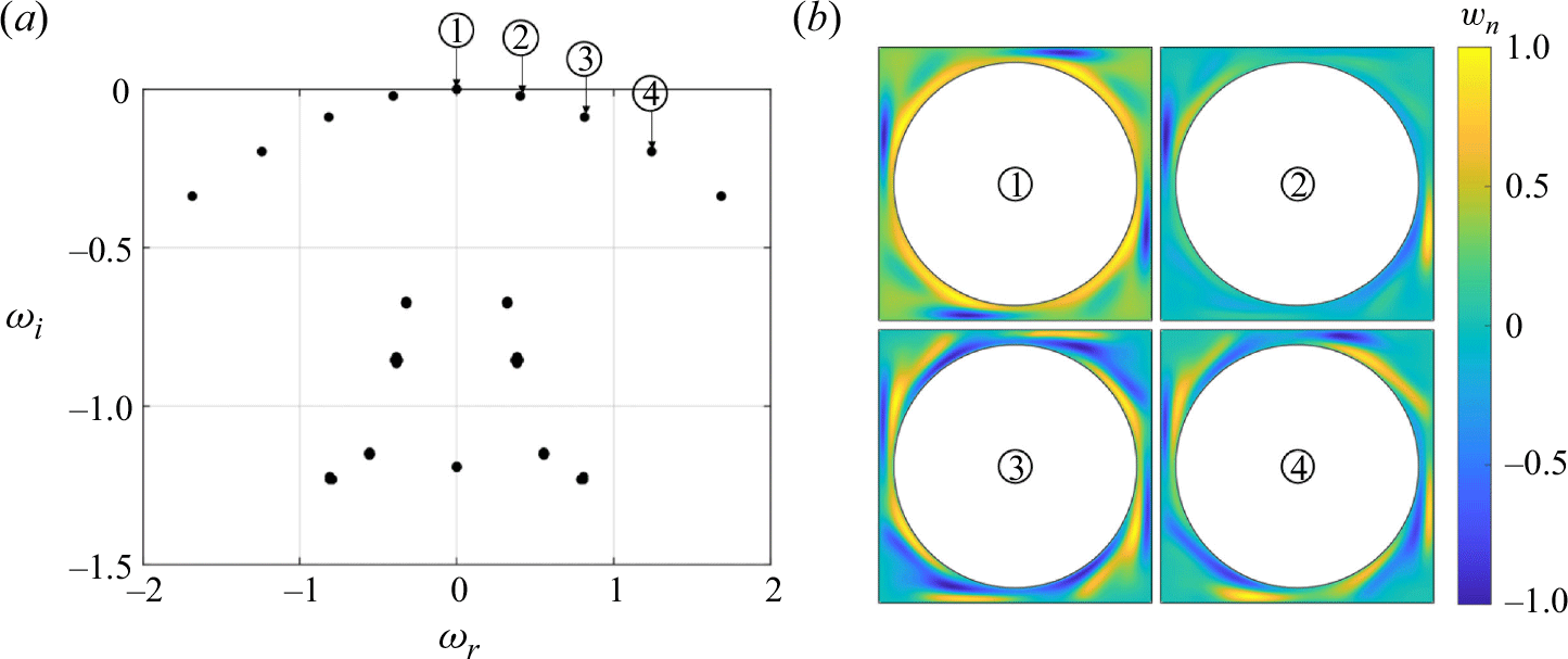
Figure 23. Eigenvalue spectrum and mode shapes for $\varDelta /d=1/16$
mm at the critical Reynolds number
$\varDelta /d=1/16$
mm at the critical Reynolds number $Re_c=586.7$
and critical wavenumber
$Re_c=586.7$
and critical wavenumber $\alpha _c=15.3$
. (a) Eigenvalue spectrum of complex frequencies
$\alpha _c=15.3$
. (a) Eigenvalue spectrum of complex frequencies $\omega = \omega _r + {\rm i} \omega _i$
, with the imaginary axis corresponding to the growth rate of the mode, and the real axis representing frequency. (b) Eigenmodes represented by contours of normalised axial velocity.
$\omega = \omega _r + {\rm i} \omega _i$
, with the imaginary axis corresponding to the growth rate of the mode, and the real axis representing frequency. (b) Eigenmodes represented by contours of normalised axial velocity.
The eigenvalue spectrum corresponding to the $\varDelta /d=1/4$
case at critical Reynolds number
$\varDelta /d=1/4$
case at critical Reynolds number $Re_c=116.4$
and critical axial wavenumber
$Re_c=116.4$
and critical axial wavenumber $\alpha _c = 4.82$
is illustrated in figure 21 along with the mode shapes of the first four modes. These modes, represented by normalised axial velocity, exhibit a rotational symmetry (figure 21
b). The first mode, which is the most unstable mode, is a Taylor-vortex-type mode that fills the gaps and corners, expanding and contracting with the available space. The radial and tangential velocity profiles at multiple radial and angular locations are shown in figure 22. The first mode closely resembles the axisymmetric mode from the canonical case, although there is a difference in the tangential velocity profile along the azimuthal direction with wave-like features.
$\alpha _c = 4.82$
is illustrated in figure 21 along with the mode shapes of the first four modes. These modes, represented by normalised axial velocity, exhibit a rotational symmetry (figure 21
b). The first mode, which is the most unstable mode, is a Taylor-vortex-type mode that fills the gaps and corners, expanding and contracting with the available space. The radial and tangential velocity profiles at multiple radial and angular locations are shown in figure 22. The first mode closely resembles the axisymmetric mode from the canonical case, although there is a difference in the tangential velocity profile along the azimuthal direction with wave-like features.
Figure 23 shows the modes present in the minimum gap case $\varDelta /d=1/16$
. The critical Reynolds number was
$\varDelta /d=1/16$
. The critical Reynolds number was $Re_c = 586.7$
at a critical axial wavenumber
$Re_c = 586.7$
at a critical axial wavenumber $\alpha _c = 15.3$
. The variation of the area from corner to corner of the square significantly affects the magnitude of the axial velocity. Similar to the
$\alpha _c = 15.3$
. The variation of the area from corner to corner of the square significantly affects the magnitude of the axial velocity. Similar to the $\varDelta /d=1/4$
case, the
$\varDelta /d=1/4$
case, the $\varDelta /d=1/16$
case also exhibits modes with azimuthal wavenumbers of integer values for the first four modes (figures 21and 23) at radial locations close to the cylinder. This spectrum closely resembles that of the simple TC flow between concentric cylinders.
$\varDelta /d=1/16$
case also exhibits modes with azimuthal wavenumbers of integer values for the first four modes (figures 21and 23) at radial locations close to the cylinder. This spectrum closely resembles that of the simple TC flow between concentric cylinders.
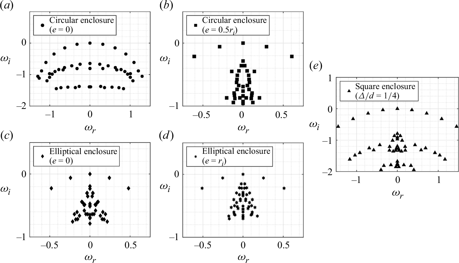
Figure 24. Eigenvalue spectrum at critical Reynolds number for the Couette flow between (a) concentric cylinders, (b) eccentric circular cylinders with eccentricity $e = 0.5$
, (c) an elliptical enclosure and concentrically placed inner circular cylinder, (d) an elliptical enclosure and an eccentrically placed inner cylinder of eccentricity
$e = 0.5$
, (c) an elliptical enclosure and concentrically placed inner circular cylinder, (d) an elliptical enclosure and an eccentrically placed inner cylinder of eccentricity $e = 0.5r_i$
, and (e) a circular cylinder and square enclosure. (Refer to Unnikrishnan et al. (Reference Unnikrishnan, Narayanan and Vanka2024b
) for details about the circular and elliptical enclosures.) All the cases have outer cylinder kept stationary.
$e = 0.5r_i$
, and (e) a circular cylinder and square enclosure. (Refer to Unnikrishnan et al. (Reference Unnikrishnan, Narayanan and Vanka2024b
) for details about the circular and elliptical enclosures.) All the cases have outer cylinder kept stationary.
The most unstable modes, marked as modes 1 to 4 on the spectrum, belong to the inverted U-shaped spectrum curve and are identified as wall modes governed by the rotation of the cylinder. The other modes present in the inner part of the spectrum are observed to be corner modes, governed by secondary flow or flow close to the outer cylinder. This new spectral branch was previously observed in the stability analysis of TC flows in circular and elliptical enclosure (Unnikrishnan et al. Reference Unnikrishnan, Narayanan and Vanka2024b ). From figure 24, it could be deduced that the introduction of eccentric placement of the inner cylinder or the ellipticity of the outer cylinder brings about a major change in the spectral branches in comparison to the Couette flow between concentric cylinders. These changes introduce a secondary flow within the domain in the form of a recirculation region. With eccentricity and ellipticity, an adverse pressure gradient is induced between the cylinders in the flow direction, creating the recirculation region. The square enclosure introduces a similar separation region at the corners. It seems that the symmetric nature of the flow within a square enclosure produces a similar spectrum compared to the spectrum of modes for Couette flow between concentric cylinders – however, with the additional modes generated by the separation region similar to the spectrum for eccentric and elliptical cases. A closer look is required to understand this spectral branch, which will be studied in future work. These different sets of modes are similar to the presence of different lines (wall modes and centre modes) in the eigenvalue spectrum from the stability analysis of Hagen–Poiseuille flow (Schmid & Henningson Reference Schmid and Henningson2001).
Appendix C. Meshless interpolation
Meshless methods do not involve element or node connectivity. Such a method represents a complex geometry only by a set of scattered points, and interpolates variables using radial basis functions (RBF). The absence of a shape parameter makes the polyharmonic spline (PHS) attractive for interpolation (Flyer et al. Reference Flyer, Fornberg, Bayona and Barnett2016; Bayona et al. Reference Bayona, Flyer, Fornberg and Barnett2017). This method does not require control volumes and element connectivity; its accuracy is not adversely affected by the skewness of the grid (Shahane & Vanka Reference Shahane and Vanka2023). Further, the PHS-RBF is appended with a polynomial, which controls the order of interpolation accuracy and the spatial derivatives (Shahane et al. Reference Shahane, Radhakrishnan and Vanka2021). A cloud-based interpolation is used with the PHS-RBF (Bartwal et al. Reference Bartwal, Shahane, Roy and Vanka2022; Unnikrishnan et al. Reference Unnikrishnan, Shahane, Narayanan and Vanka2022; Unnikrishnan et al. Reference Unnikrishnan, Narayanan, Chamorro and Vanka2024a
) for the present analysis. An arbitrary variable $s(\boldsymbol{x})$
is interpolated as
$s(\boldsymbol{x})$
is interpolated as
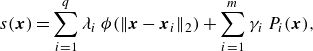 \begin{equation} s(\boldsymbol{x}) = \sum _{i=1}^{q} \lambda _i\, \phi (\|\boldsymbol{x} - \boldsymbol{x}_i\|_2) + \sum _{i=1}^{m} \gamma _i\, P_i (\boldsymbol{x}), \end{equation}
where $\phi (r)=r^{2a+1},\ a \in \mathbb{N}$
, is the PHS-RBF,
$\phi (r)=r^{2a+1},\ a \in \mathbb{N}$
, is the PHS-RBF, $m$
is the number of monomials (
$m$
is the number of monomials ( $P_i$
) up to maximum degree
$P_i$
) up to maximum degree $l$
, and
$l$
, and $(\lambda _i, \gamma _i)$
are
$(\lambda _i, \gamma _i)$
are $q+m$
coefficients. We use
$q+m$
coefficients. We use $a =1$
, and
$a =1$
, and $q$
equations are obtained by collocating (C1) over the
$q$
equations are obtained by collocating (C1) over the $q$
cloud points. The power of the PHS function is found to have only a weak effect on the accuracy of interpolation. The
$q$
cloud points. The power of the PHS function is found to have only a weak effect on the accuracy of interpolation. The $m$
additional equations required to close the linear system are imposed as constraints on the polynomials (Flyer et al. Reference Flyer, Fornberg, Bayona and Barnett2016):
$m$
additional equations required to close the linear system are imposed as constraints on the polynomials (Flyer et al. Reference Flyer, Fornberg, Bayona and Barnett2016):
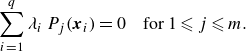 \begin{equation} \sum _{i=1}^{q} \lambda _i\, P_j(\boldsymbol{x}_i) =0 \quad \text{for } 1 \leqslant j \leqslant m. \end{equation}
In a matrix–vector form, we can write these equations as
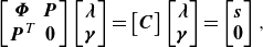 \begin{equation} \begin{bmatrix} \boldsymbol{\Phi } & \boldsymbol{P} \\ \boldsymbol{P}^T & \boldsymbol{0} \\ \end{bmatrix} \begin{bmatrix} \boldsymbol{\lambda } \\ \boldsymbol{\gamma } \\ \end{bmatrix} = \begin{bmatrix} \boldsymbol{C} \end{bmatrix} \begin{bmatrix} \boldsymbol{\lambda } \\ \boldsymbol{\gamma } \\ \end{bmatrix} = \begin{bmatrix} \boldsymbol{s} \\ \boldsymbol{0} \\ \end{bmatrix}, \end{equation}
where transpose is denoted by the superscript ${\rm T}$
,
${\rm T}$
, $\boldsymbol{\lambda } = [\lambda _1,\ldots ,\lambda _q]^{\rm T}$
,
$\boldsymbol{\lambda } = [\lambda _1,\ldots ,\lambda _q]^{\rm T}$
, $\boldsymbol{\gamma } = [\gamma _1,\ldots ,\gamma _m]^{\rm T}$
,
$\boldsymbol{\gamma } = [\gamma _1,\ldots ,\gamma _m]^{\rm T}$
, $\boldsymbol{s} = [s(\boldsymbol{x}_1),\ldots ,s(\boldsymbol{x}_q)]^{\rm T}$
, and
$\boldsymbol{s} = [s(\boldsymbol{x}_1),\ldots ,s(\boldsymbol{x}_q)]^{\rm T}$
, and $\boldsymbol{0}$
is the vector of zeros. Dimensions of the submatrices
$\boldsymbol{0}$
is the vector of zeros. Dimensions of the submatrices $\boldsymbol{\Phi }$
and
$\boldsymbol{\Phi }$
and $\boldsymbol{P}$
are
$\boldsymbol{P}$
are $q\times q$
and
$q\times q$
and $q\times m$
, respectively.
$q\times m$
, respectively.
In two-dimensional problems with appended polynomial of degree 2, there are $m=6$
polynomial terms, given as
$m=6$
polynomial terms, given as $[1, x, y, x^2, xy, y^2]$
. For our computations, we have used appended polynomials of degree 5. The accuracy of the first derivative is the same as the polynomial degree, and the accuracy of the second derivative is 1 less than the polynomial degree (Shahane et al. Reference Shahane, Radhakrishnan and Vanka2021). With the fifth degree of appended polynomial, the first derivative has order of accuracy 5, and the second derivative has order of accuracy 4. The differential operators (
$[1, x, y, x^2, xy, y^2]$
. For our computations, we have used appended polynomials of degree 5. The accuracy of the first derivative is the same as the polynomial degree, and the accuracy of the second derivative is 1 less than the polynomial degree (Shahane et al. Reference Shahane, Radhakrishnan and Vanka2021). With the fifth degree of appended polynomial, the first derivative has order of accuracy 5, and the second derivative has order of accuracy 4. The differential operators ( $\mathcal{D}$
) can be obtained by differentiating the RBF and the polynomials:
$\mathcal{D}$
) can be obtained by differentiating the RBF and the polynomials:
 \begin{equation} \mathcal{D} [s(\boldsymbol{x})] = \sum _{i=1}^{q} \lambda _i\, \mathcal{D} [\phi (\boldsymbol{\|\boldsymbol{x} - \boldsymbol{x}_i\|_2})] + \sum _{i=1}^{m} \gamma _i\, \mathcal{D}[P_i (\boldsymbol{x})]. \end{equation}
Equation (C4) applied to all the points in the cloud leads to a rectangular matrix–vector system given by
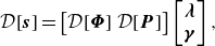 \begin{equation} \mathcal{D}[\boldsymbol{s}] = \begin{bmatrix} \mathcal{D}[\boldsymbol{\Phi }] & \mathcal{D}[\boldsymbol{P}] \\ \end{bmatrix} \begin{bmatrix} \boldsymbol{\lambda } \\ \boldsymbol{\gamma } \\ \end{bmatrix}, \end{equation}
where $\mathcal{D}[\boldsymbol{\Phi }]$
and
$\mathcal{D}[\boldsymbol{\Phi }]$
and $\mathcal{D}[\boldsymbol{P}]$
are matrices of sizes
$\mathcal{D}[\boldsymbol{P}]$
are matrices of sizes $q\times q$
and
$q\times q$
and $q\times m$
, respectively. Substituting (C3) in (C5) results in
$q\times m$
, respectively. Substituting (C3) in (C5) results in
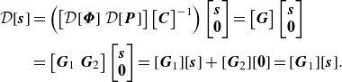 \begin{equation} \begin{aligned} \mathcal{D}[\boldsymbol{s}] &= \left (\begin{bmatrix} \mathcal{D}[\boldsymbol{\Phi }] & \mathcal{D}[\boldsymbol{P}] \\ \end{bmatrix} \begin{bmatrix} \boldsymbol{C} \end{bmatrix} ^{-1}\right ) \begin{bmatrix} \boldsymbol{s} \\ \boldsymbol{0} \\ \end{bmatrix} = \begin{bmatrix} \boldsymbol{G} \end{bmatrix} \begin{bmatrix} \boldsymbol{s} \\ \boldsymbol{0} \\ \end{bmatrix}\\ &= \begin{bmatrix} \boldsymbol{G}_1 & \boldsymbol{G}_2 \end{bmatrix} \begin{bmatrix} \boldsymbol{s} \\ \boldsymbol{0} \\ \end{bmatrix} = [\boldsymbol{G}_1] [\boldsymbol{s}] + [\boldsymbol{G}_2] [\boldsymbol{0}] = [\boldsymbol{G}_1] [\boldsymbol{s}]. \end{aligned} \end{equation}
From (C6), any differential operator $\mathcal{D}$
is approximated by a matrix
$\mathcal{D}$
is approximated by a matrix $\boldsymbol{G}_1$
that multiplies the discrete values of the variable
$\boldsymbol{G}_1$
that multiplies the discrete values of the variable $s$
. By substituting the expressions for the operators in (B1), we can now generate the complete
$s$
. By substituting the expressions for the operators in (B1), we can now generate the complete $\boldsymbol{A}$
and
$\boldsymbol{A}$
and $\boldsymbol{B}$
matrices for given values of wavenumber
$\boldsymbol{B}$
matrices for given values of wavenumber $\alpha$
and
$\alpha$
and $Re$
.
$Re$
.


 Open access