


1. Introduction
One of the most celebrated instabilities in fluid dynamics is the Benjamin–Feir instability, where a Stokes wavetrain, travelling uniformly in finite depth, undergoes a transition from stability to instability as the depth of the fluid increases. The original papers (Benjamin Reference Benjamin1967; Benjamin & Feir Reference Benjamin and Feir1967) have attracted significant attention in the years since their first publication. Nevertheless it continues to fascinate, and there is still much to learn about its implications. One such phenomenon, known now as frequency downshifting, emerged in experiments following up on the Benjamin–Feir result. These experimental investigations of monochromatic wavetrains (e.g. Lake et al. Reference Lake, Yuen, Rungaldier and Ferguson1977; Melville Reference Melville1982; Su et al. Reference Su, Bergin, Marler and Myrick1982; Huang, Long & Shen Reference Huang, Long and Shen1996) demonstrated that energy is exchanged from the primary wave mode to other sideband frequencies. As this process begins to arrest, these experiments observed that the dominant peak of the wave power occurred not at the original carrier-wave frequency, but one of a lower frequency, namely that the frequency peak had moved down the spectrum to lower frequencies (and thus the nomenclature). In this paper we focus on modulation and dynamics of water waves near the Benjamin–Feir transition, and find that the frequency downshifting phenomenon emerges naturally via phase dynamics.
The conventional explanation as to how this phenomenon emerges is via dissipative effects, such as wind forcing or inherent viscous effects, and these explanations have been supported by numerical simulations (Lo & Mei Reference Lo and Mei1985; Hara & Mei Reference Hara and Mei1991; Dias & Kharif Reference Dias and Kharif1999; Carter & Govan Reference Carter and Govan2016; Carter, Henderson & Butterfield Reference Carter, Henderson and Butterfield2019). It was thought that permanent frequency downshifting was not possible in purely conservative systems (Lo & Mei Reference Lo and Mei1985; Hara & Mei Reference Hara and Mei1991; Dias & Kharif Reference Dias and Kharif1999). However, as with all nonlinear paradigms, more than one mechanism can lead to the same phenomenon. There is a growing consensus that frequency downshifting can indeed be observed without energy dissipation or forcing (Onorato et al. Reference Onorato, Osborne, Serio, Resio, Pushkarev, Zakharov and Brandini2002; Dysthe et al. Reference Dysthe, Trulsen, Krogstad and Socquet-Juglard2003; Janssen Reference Janssen2003; Chalikov Reference Chalikov2007, Reference Chalikov2012; Shugan et al. Reference Shugan, Kuznetsov, Saprykina, Hwung, Yang and Chen2019). Whilst some of these alternative mechanisms have been observed numerically, an open question remains as to the theoretical explanation for downshifting to occur without dissipation.
In this paper we propose a new mechanism for frequency downshifting for inviscid and irrotational water waves without dissipation. The theory is based on asymptotically valid modulation equations, building on classical Whitham modulation theory and its generalisations. Whitham modulation theory has a distinct advantage over nonlinear Schrödinger equation models (e.g. Hasimoto & Ono Reference Hasimoto and Ono1972; Johnson Reference Johnson1977; Kakutani & Michihiro Reference Kakutani and Michihiro1983) in that it is precisely the wavenumber and frequency that are modulated, thereby generating equations that inherently contain jumps in frequency. In the conservative setting, it is singularities that provide the mechanism for downshifting. The primary singularity is coalescence of two characteristics in the Whitham modulation equations at the Benjamin–Feir transition (Whitham Reference Whitham1967).
One has to go beyond Whitham (Reference Whitham1967) as higher-order modulation equations are required in order to capture the nonlinear implications of the double characteristic, which is what we achieve here within this paper. Our strategy is to re-scale and re-modulate to obtain new asymptotically valid modulation equations near the Benjamin–Feir threshold. In Bridges & Ratliff (Reference Bridges and Ratliff2017, Reference Bridges and Ratliff2021) a general theory for the re-modulation of Whitham theory in the neighbourhood of coalescing characteristics is constructed. There it is found that the conservation of wave action in Whitham theory is instead replaced by a two-way Boussinesq equation for the modulation wavenumber, with the modulation frequency coming in via the equation for conservation of waves. However, this theory needs modification as a secondary singularity arises at the Benjamin–Feir transition, changing the nonlinearity in the two-way Boussinesq equation from quadratic to cubic. The resulting modulation equation, first derived in Ratliff (Reference Ratliff2017), is
 \begin{equation} \alpha _1U_{\textit{TT}} +\alpha _2(U^3)_{\textit{XX}}+\alpha _3(2UU_T+U_X\partial _X^{-1}U_T)_X + \alpha _4 U_{\textit{XXXX}} = 0\,, \end{equation}
where $U$
characterises the local wavenumber,
$U$
characterises the local wavenumber, $T,X$
are slow time and space scales and
$T,X$
are slow time and space scales and $\alpha _1,\ldots ,\alpha _4$
are real-valued parameters. It is the key equation in this paper, as it is asymptotically valid and contains travelling fronts which connect two wavenumber states thereby capturing the frequency downshifting via conservation of waves. The properties and analysis of (1.1) are given in § 4.
$\alpha _1,\ldots ,\alpha _4$
are real-valued parameters. It is the key equation in this paper, as it is asymptotically valid and contains travelling fronts which connect two wavenumber states thereby capturing the frequency downshifting via conservation of waves. The properties and analysis of (1.1) are given in § 4.
There are several steps in the analysis leading from the generic Whitham theory to (1.1). The first step is to introduce a general form for the secondary modulation of the Stokes wave and mean flow. The form of the phase, wavenumber and frequency modulation is cast in vector form as
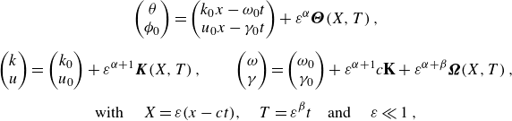 \begin{equation} \begin{gathered} \begin{pmatrix} \theta \\ \phi _0 \end{pmatrix} = \begin{pmatrix} k_0x-\omega _0t\\ u_0x-\gamma _0t \end{pmatrix} +\varepsilon ^\alpha \boldsymbol{\Theta }(X,T)\,, \\[5pt] \begin{pmatrix} k\\ u \end{pmatrix} = \begin{pmatrix} k_0\\ u_0 \end{pmatrix}+\varepsilon ^{\alpha +1}\boldsymbol{K}(X,T)\,,\qquad \begin{pmatrix} \omega \\ \gamma \end{pmatrix} = \begin{pmatrix} \omega _0\\ \gamma _0 \end{pmatrix}+\varepsilon ^{\alpha +1} c \textbf{K}+\varepsilon ^{\alpha +\beta }\boldsymbol{\Omega }(X,T)\,,\\[5pt] \textrm {with } \quad X = \varepsilon (x-ct), \quad T = \varepsilon ^\beta t \quad \textrm {and } \quad \varepsilon \ll 1\,, \end{gathered} \end{equation}
where $k_0,\omega _0$
are the wavenumber and frequency of the Stokes wave and
$k_0,\omega _0$
are the wavenumber and frequency of the Stokes wave and $u_0,\gamma _0$
are the bulk velocity and Bernoulli constant of the mean flow. The speed
$u_0,\gamma _0$
are the bulk velocity and Bernoulli constant of the mean flow. The speed $c$
is a characteristic speed obtained from the generic Whitham modulation equations using the standard approach (Whitham Reference Whitham2011). The quantity
$c$
is a characteristic speed obtained from the generic Whitham modulation equations using the standard approach (Whitham Reference Whitham2011). The quantity $\theta$
is the phase of the wave, and
$\theta$
is the phase of the wave, and $\phi _0$
is referred to as the pseudo-phase of the mean flow, due to its resemblance to a wave phase and playing a similar role in the Whitham modulation equation. The exponents
$\phi _0$
is referred to as the pseudo-phase of the mean flow, due to its resemblance to a wave phase and playing a similar role in the Whitham modulation equation. The exponents $\alpha$
and
$\alpha$
and $\beta$
are determined by ensuring that the equations are asymptotically valid, and that the modulation wavenumber and frequencies are in balance:
$\beta$
are determined by ensuring that the equations are asymptotically valid, and that the modulation wavenumber and frequencies are in balance:
 \begin{align} {\boldsymbol{\Theta }}_X = {\boldsymbol{K}} \quad \textrm {and} \quad {\boldsymbol{\Theta }}_T = -\boldsymbol{\Omega }\,. \end{align}
We will look at two cases of the re-modulation. The first is with scales $\alpha =1$
and
$\alpha =1$
and $\beta =3$
. These values are relevant in the hyperbolic region, where all four characteristics in Whitham (Reference Whitham1967) are real, and
$\beta =3$
. These values are relevant in the hyperbolic region, where all four characteristics in Whitham (Reference Whitham1967) are real, and
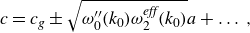 \begin{align} c = c_g \pm \sqrt {\omega^{\prime\prime}_0(k_0) \omega _2^{\textit{eff}}(k_0)} a+\ldots \,, \end{align}
with $\omega^{\prime\prime}_0\omega _2^{\textit{eff}}\gt 0$
, where
$\omega^{\prime\prime}_0\omega _2^{\textit{eff}}\gt 0$
, where $a$
denotes the wave amplitude and
$a$
denotes the wave amplitude and $\omega _2^{\textit{eff}}$
is the (Stokes) frequency correction to the Stokes wave, including mean flow. In this region we find that re-modulation leads to Korteweg de-Vries (KdV) dynamics, with the modulation equation taking the universal form (Ratliff Reference Ratliff2021)
$\omega _2^{\textit{eff}}$
is the (Stokes) frequency correction to the Stokes wave, including mean flow. In this region we find that re-modulation leads to Korteweg de-Vries (KdV) dynamics, with the modulation equation taking the universal form (Ratliff Reference Ratliff2021)
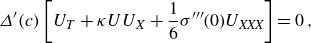 \begin{equation} \varDelta ^{\prime}(c) \left [U_T+\kappa UU_X+\frac {1}{6}\sigma^{\prime\prime\prime}(0)U_{\textit{XXX}}\right ] = 0\,, \end{equation}
with $U$
characterising the evolution of the vector-valued wavenumber via
$U$
characterising the evolution of the vector-valued wavenumber via ${\boldsymbol{K}} = \zeta U(X,T)$
and
${\boldsymbol{K}} = \zeta U(X,T)$
and $\zeta$
is the right eigenvector of the Whitham modulation equations. Thus, the re-modulation slaves the slow evolution of the wave and mean flow to one another within the water-wave problem. The new modulation dynamics is characterised by properties of the wavetrain via the characteristic polynomial of the Whitham modulation equations
$\zeta$
is the right eigenvector of the Whitham modulation equations. Thus, the re-modulation slaves the slow evolution of the wave and mean flow to one another within the water-wave problem. The new modulation dynamics is characterised by properties of the wavetrain via the characteristic polynomial of the Whitham modulation equations $\varDelta (c)$
and the Bloch spectrum of the wave
$\varDelta (c)$
and the Bloch spectrum of the wave $\sigma (\nu )$
(Doelman et al. Reference Doelman, Sandstede, Scheel and Schneider2009). The coefficient of the quadratic nonlinearity is
$\sigma (\nu )$
(Doelman et al. Reference Doelman, Sandstede, Scheel and Schneider2009). The coefficient of the quadratic nonlinearity is
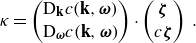
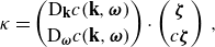 \begin{align} \kappa = \begin{pmatrix} \textrm {D}_{\textbf{k}} c(\textbf{k},\boldsymbol{\omega })\\[3pt] \textrm {D}_{\boldsymbol{\omega }} c(\textbf{k},\boldsymbol{\omega }) \end{pmatrix} \cdot \begin{pmatrix} \boldsymbol{\zeta }\\[3pt] c \boldsymbol{\zeta } \end{pmatrix}\,, \end{align}
where $c(\textbf{k},\boldsymbol{\omega })$
is a modulation (characteristic) speed and
$c(\textbf{k},\boldsymbol{\omega })$
is a modulation (characteristic) speed and $\textrm {D}$
denotes a directional (Gateaux) derivative, which can be interpreted as the linearised version of Lax’s genuine nonlinearity criterion for the Whitham modulation equations (Ratliff Reference Ratliff2021). The analysis leading to this equation, as well as the definitions of
$\textrm {D}$
denotes a directional (Gateaux) derivative, which can be interpreted as the linearised version of Lax’s genuine nonlinearity criterion for the Whitham modulation equations (Ratliff Reference Ratliff2021). The analysis leading to this equation, as well as the definitions of $\varDelta (c)$
and Bloch spectrum
$\varDelta (c)$
and Bloch spectrum $\sigma (\nu )$
, are given in § 3.
$\sigma (\nu )$
, are given in § 3.
It is important to note that the KdV equation (1.5) is not the famous KdV equation in shallow-water hydrodynamics (Korteweg & De Vries Reference Korteweg and De Vries1895)! It is a KdV equation describing perturbations of the Stokes wave and the mean flow, and not just long-wave perturbations to the free surface and velocity (i.e. just the mean flow in the absence of a background wave). This KdV equation is of interest here because in the limit to the Benjamin–Feir transition, the coefficient $\kappa$
of the quadratic nonlinearity goes to zero, signalling the change from quadratic to cubic nonlinearity. This KdV equation may also have independent interest in giving an alternative explanation for the appearance of dark solitary waves in shallow-water hydrodynamics (cf. Bridges & Donaldson Reference Bridges and Donaldson2006).
$\kappa$
of the quadratic nonlinearity goes to zero, signalling the change from quadratic to cubic nonlinearity. This KdV equation may also have independent interest in giving an alternative explanation for the appearance of dark solitary waves in shallow-water hydrodynamics (cf. Bridges & Donaldson Reference Bridges and Donaldson2006).
In summary, the argument for frequency downshifting takes three steps. Firstly, generic Whitham modulation theory gives the characteristics with two of these changing type from hyperbolic to elliptic at the Benjamin–Feir transition. Secondly, re-modulation in the hyperbolic region generates KdV dynamics on top of the Stokes wave and mean flow. Taking the limit to the Benjamin–Feir transition then leads to a third modulation equation (1.1) for the wavenumber, and its jump solutions generate frequency downshifting (or, in principle, upshifting). Whilst this paper will focus on the water-wave problem as the key application of the above abstract theory, the theory is more general as it applies to a basic periodic wavetrain of any amplitude, as long as it has at least two phases. The secondary modulation then is applicable. This form of frequency downshifting is universal in that the theory is formulated independent of any particular equation, as long as it is conservative and generated by a Lagrangian. However, in this paper the focus is on the Benjamin–Feir transition.
An outline of the paper is as follows. In § 2 the theory for re-modulation is set up and those aspects of Whitham (Reference Whitham1967) that feed into the higher-order modulation equations are highlighted. Then in § 3 the KdV equation on a Stokes wave (1.5) is derived and analysed. It is valid everywhere in the hyperbolic region of generic Whitham theory, and we are interested in its behaviour near the hyperbolic–elliptic transition which signals the onset of Benjamin–Feir instability. In § 3 we also introduce the concept of Bloch spectrum which arises in the derivation of the dispersive term both in (1.5) and in (1.1). In § 4 the key properties of (1.1) are highlighted, and the analysis leading to jumps in wavenumber and frequency is given. Further support for the new theory of frequency downshifting is presented in § 5 using energy arguments, and in § 6 by direct simulation of the Benney–Roskes equation. We find that the downshifted wavetrain is the state with the lower energy, providing an energetic argument for why downshifting is observed and persistent even in conservative systems. In the concluding remarks section we summarise the main result, and indicate some generalisations.
2. Stokes waves, modulation and characteristics
In this section, we set up the basic state and its properties. The basic state is a Stokes wave on finite depth coupled to mean flow. The starting point for the analysis is the inviscid, irrotational model for gravity waves in finite depth $h_0$
and constant density. The governing equations for the velocity potential
$h_0$
and constant density. The governing equations for the velocity potential $\phi (x,y,t)$
and the free surface deflection
$\phi (x,y,t)$
and the free surface deflection $\eta (x,t)$
on the domain
$\eta (x,t)$
on the domain $(x,y,t) \in {\mathbb{R}}\times [-h_0,\eta ]\times [0,\infty )$
are
$(x,y,t) \in {\mathbb{R}}\times [-h_0,\eta ]\times [0,\infty )$
are
 \begin{align} \phi _{\textit{xx}}+\phi _{\textit{yy}} &= 0\,,\quad \mbox{for}\ y \in (-h_0,\eta )\,, \end{align}
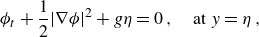
 \begin{align} \phi _y(x,-h_0,t) &= 0\,, \end{align}
 \begin{align} \eta _t+\phi _x\eta _x &= \phi _y\,,\quad \mbox{at}\ y = \eta \,, \end{align}
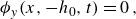
 \begin{align} \phi _t+\frac{1}{2}|\nabla \phi |^2+g \eta &= 0\,, \quad \mbox{at}\ y = \eta \,, \end{align}
where $g$
is the acceleration due to gravity. These equations are conservative and can be obtained from the first variation of a Lagrangian:
$g$
is the acceleration due to gravity. These equations are conservative and can be obtained from the first variation of a Lagrangian:
 \begin{equation} \delta L =0\,,\quad \mbox{with } \quad L= \int \int \left (\int _{-h_0}^\eta \phi _t+\frac{1}{2}|\nabla \phi |^2+g y\ {\textrm d}y\right )\ {\textrm d}x\,{\textrm d}t. \end{equation}
The evaluation of $\delta L=0$
is given in § 13.2 of Whitham (Reference Whitham2011). Now consider a Stokes expansion for the velocity potential and free surface:
$\delta L=0$
is given in § 13.2 of Whitham (Reference Whitham2011). Now consider a Stokes expansion for the velocity potential and free surface:
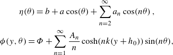 \begin{align} \begin{gathered} \eta (\theta ) = b+a \cos (\theta )+\sum _{n=2}^\infty a_n\cos (n \theta )\,, \\ \phi (y,\theta ) = \varPhi +\sum _{n=1}^\infty \frac {A_n}{n}\cosh (nk(y+h_0) )\sin (n\theta ), \end{gathered} \end{align}
with phases $\theta$
and
$\theta$
and $\varPhi$
given by
$\varPhi$
given by
 \begin{align} \theta = kx-\omega t\quad \mbox{and}\quad \varPhi = ux-\gamma t\,. \end{align}
The constants $k,\,\omega$
(representing the wavenumber and frequency) and
$k,\,\omega$
(representing the wavenumber and frequency) and $u,\,\gamma$
(representing the horizontal fluid velocity and Bernoulli head) parametrise the wave and the mean flow, respectively. The parameters
$u,\,\gamma$
(representing the horizontal fluid velocity and Bernoulli head) parametrise the wave and the mean flow, respectively. The parameters $a$
and
$a$
and $b$
parametrise the amplitudes of the surface Stokes wave and mean fluid deflection from rest (i.e.
$b$
parametrise the amplitudes of the surface Stokes wave and mean fluid deflection from rest (i.e. $\eta =0$
), respectively.
$\eta =0$
), respectively.
The quantity $\theta$
is the usual phase of the wavetrain, whereas
$\theta$
is the usual phase of the wavetrain, whereas $\varPhi$
is called a pseudo-phase, although mathematically it is equivalent to the wave phase (cf. § 3.1 in Bridges & Ratliff (Reference Bridges and Ratliff2021)). The pseudo-phase arises from an affine symmetry in
$\varPhi$
is called a pseudo-phase, although mathematically it is equivalent to the wave phase (cf. § 3.1 in Bridges & Ratliff (Reference Bridges and Ratliff2021)). The pseudo-phase arises from an affine symmetry in $\phi$
present in the Lagrangian. The above solution, therefore, can be treated as a relative equilibrium with two phases – one associated with the translation invariance in phase of the Lagrangian, and the other due to the affine symmetry of the velocity potential. The presence of these mean flow effects facilitates the inclusion of the bulk mode
$\phi$
present in the Lagrangian. The above solution, therefore, can be treated as a relative equilibrium with two phases – one associated with the translation invariance in phase of the Lagrangian, and the other due to the affine symmetry of the velocity potential. The presence of these mean flow effects facilitates the inclusion of the bulk mode $b$
in the expansion of
$b$
in the expansion of $\eta$
, which alters the mean (i.e. period-averaged) fluid depth to
$\eta$
, which alters the mean (i.e. period-averaged) fluid depth to $h_0+b$
in response to mean-flow effects primarily driven by
$h_0+b$
in response to mean-flow effects primarily driven by $u$
and
$u$
and $\gamma$
. This therefore leads to two ‘triads’ in the modulation theory –
$\gamma$
. This therefore leads to two ‘triads’ in the modulation theory – $(k,\omega ,a)$
characterising the surface Stokes wave and
$(k,\omega ,a)$
characterising the surface Stokes wave and $(u,\gamma ,b)$
for the mean-flow effects. As we will see within this paper, the two triads couple, and it is this coupling that drives the dynamics which leads to downshifting in the vicinity of the Benjamin–Feir instability.
$(u,\gamma ,b)$
for the mean-flow effects. As we will see within this paper, the two triads couple, and it is this coupling that drives the dynamics which leads to downshifting in the vicinity of the Benjamin–Feir instability.
Substitution of the above wave–mean-flow solution into the Lagrangian, averaging over one period of the wave and solving the resulting system of equations for the Fourier coefficients $a_n$
and
$a_n$
and $A_n$
, one is able to obtain the following averaged Lagrangian, to leading order in
$A_n$
, one is able to obtain the following averaged Lagrangian, to leading order in $E$
and
$E$
and $b$
:
$b$
:
 \begin{align} {\mathscr{L}} = \left (\frac {u^{2}}{2}-\gamma \right )(h_0+b)+\frac{1}{2}g b^{2}+D(k,u,\omega ) E+\mu E \ b +\frac{1}{2}\tau E^{2} +{\mathcal{O}} \big(b^{2},E^{3}, E^{2} b\big)\,.\nonumber\\ \end{align}
The two small parameters are the energy density $E = ({1}/{2})g a^{2}$
and mean deflection
$E = ({1}/{2})g a^{2}$
and mean deflection $b$
from the quiescent position
$b$
from the quiescent position $\eta = 0$
. This reduced Lagrangian is derived in Whitham (Reference Whitham1967) and has been confirmed in Bridges & Ratliff (Reference Bridges and Ratliff2022).
$\eta = 0$
. This reduced Lagrangian is derived in Whitham (Reference Whitham1967) and has been confirmed in Bridges & Ratliff (Reference Bridges and Ratliff2022).
The function $D$
is the right-moving linear dispersion relation with a mean flow component
$D$
is the right-moving linear dispersion relation with a mean flow component
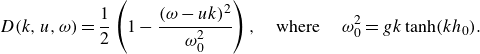 \begin{align} D(k,u,\omega ) = \frac{1}{2}\left (1-\frac {(\omega -u k)^{2}}{\omega _0^{2}} \right ), \quad \textrm {where } \quad \omega _0^{2} = gk \tanh (kh_0). \end{align}
It has a root at $\omega = uk+\omega _0(k)$
. The constants
$\omega = uk+\omega _0(k)$
. The constants $\mu$
and
$\mu$
and $\tau$
in (2.5) are
$\tau$
in (2.5) are
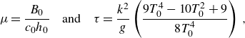 \begin{equation} \mu = \frac {B_0}{c_0h_0} \quad \mbox{and}\quad \tau = \frac {k^{2}}{g}\left (\frac {9T_0^4-10T_0^{2}+9}{8T_0^4}\right )\,, \end{equation}
with
 \begin{align} B_0 = c_g-\frac {c_0}{2}, \quad c_g = u+\omega^{\prime}_0(k),\quad c_0 = \frac {\omega _0}{k} \quad \mbox{and } \quad T_0 = \tanh (kh_0). \end{align}
Primes represent derivatives with respect to the wavenumber $k$
. Variations of the Lagrangian (2.5) with respect to
$k$
. Variations of the Lagrangian (2.5) with respect to $E$
and
$E$
and $b$
, when set to zero, yield the weakly nonlinear dispersion relations
$b$
, when set to zero, yield the weakly nonlinear dispersion relations
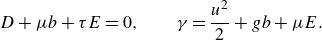 \begin{equation} D+\mu b+\tau E = 0, \qquad \gamma = \frac {u^{2}}{2} +g b+ \mu E .\end{equation}
In the absence of mean variations (i.e. $b=0$
), the first can be solved to find the conventional low-amplitude Stokes expansion of the frequency:
$b=0$
), the first can be solved to find the conventional low-amplitude Stokes expansion of the frequency:
 \begin{align} \omega = uk+{\omega _0}(k) +\omega _2^{0} E+{\mathcal{O}}(E^2), \end{align}
where the Stokes frequency correction in the absence of bulk/mean-flow variations, $\omega _2^0$
, is given by
$\omega _2^0$
, is given by
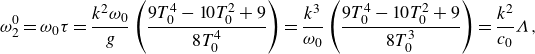 \begin{align} \omega _2^0 = \omega _0 \tau = \frac {k^{2} \omega _0}{g}\left (\frac {9T_0^4-10T_0^{2}+9}{8T_0^4}\right ) = \frac {k^{3}}{\omega _0}\left (\frac {9T_0^4-10T_0^{2}+9}{8T_0^{3}}\right ) = \frac {k^{2}}{c_0}\varLambda , \end{align}
where the expression $\varLambda$
is precisely
$\varLambda$
is precisely $D_0$
in Whitham (Reference Whitham1967), but the notation has been altered to prevent confusion. The dependence of
$D_0$
in Whitham (Reference Whitham1967), but the notation has been altered to prevent confusion. The dependence of $\omega _2^0$
on
$\omega _2^0$
on $k$
is important and will be retained here as derivatives of
$k$
is important and will be retained here as derivatives of $\omega _2^0$
with respect to these parameters appear in the analysis, at leading order. Therefore, it is convenient to establish
$\omega _2^0$
with respect to these parameters appear in the analysis, at leading order. Therefore, it is convenient to establish $\tau = \omega _0^{-1} \omega _2^0$
, and thus we may write the coupled system (2.9) as
$\tau = \omega _0^{-1} \omega _2^0$
, and thus we may write the coupled system (2.9) as
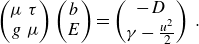 \begin{equation} \begin{pmatrix} \mu & \tau \\ g & \mu \end{pmatrix} \begin{pmatrix} b\\ E \end{pmatrix} = \begin{pmatrix} -D\\ \gamma -\frac {u^{2}}{2} \end{pmatrix}\,. \end{equation}
Henceforth, all expressions and coefficients within the paper, unless explicitly stated otherwise, will be evaluated at $\omega = uk+\omega _0(k)$
. It is assumed henceforth that these equations are non-degenerate:
$\omega = uk+\omega _0(k)$
. It is assumed henceforth that these equations are non-degenerate:
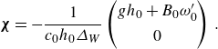
 \begin{align} \varDelta_{W} = \mu ^{2}-g \tau =\frac {B_0^{2}}{c_0^{2}h_0^{2}}-\frac {g \omega _2^0}{\omega _0} \neq 0\,. \end{align}
Indeed, this expression is negative-definite for gravity waves (but may change sign in other water-wave problems, such as when surface tension or variable density is present). This equation clearly demonstrates that the energy density $E$
and bulk variation
$E$
and bulk variation $b$
are truly independent, and not constrained as previously suggested in § 16.9 of Whitham (Reference Whitham2011). The independence of
$b$
are truly independent, and not constrained as previously suggested in § 16.9 of Whitham (Reference Whitham2011). The independence of $b$
and
$b$
and $E$
play an important role in the phase modulation of the Stokes waves, when
$E$
play an important role in the phase modulation of the Stokes waves, when $E$
and
$E$
and $b$
are slowly varying functions. The precise leading-order effect of the mean velocity field on the wave component is given in Appendix A. Further, this system prescribes
$b$
are slowly varying functions. The precise leading-order effect of the mean velocity field on the wave component is given in Appendix A. Further, this system prescribes $E$
and
$E$
and $b$
as functions of the wave and mean-flow parameters
$b$
as functions of the wave and mean-flow parameters $k,\,\omega ,\,u$
and
$k,\,\omega ,\,u$
and $\gamma$
, which are required for the phase dynamical reduction.
$\gamma$
, which are required for the phase dynamical reduction.
2.1. Modulating wave and mean flow
In classical Whitham modulation theory (Whitham Reference Whitham1967), applied to the wave mean-flow problem, the key parameters
 \begin{equation} {\boldsymbol{\Theta }} = \begin{pmatrix} \theta \\ \Phi \end{pmatrix}\,, \quad \textbf{k} = \begin{pmatrix} k\\u \end{pmatrix}\,, \quad \boldsymbol{\omega } = \begin{pmatrix} \omega \\ \gamma \end{pmatrix} \end{equation}
are allowed to be slowly varying functions:
 \begin{equation} \begin{gathered} {\boldsymbol{\theta }} \to {\boldsymbol{\theta }} +\varepsilon ^{-1}{\boldsymbol{\Theta }}(X,T)\,, \quad \textbf{k} \to \textbf{k}+{\boldsymbol{K}}(X,T)\,, \quad \boldsymbol{\omega } \to \boldsymbol{\omega }+ \boldsymbol{\Omega }(X,T)\,,\\[4pt] \textrm {where }\quad X = \varepsilon (x-ct), \quad T = \varepsilon t \quad \textrm {and } \quad \varepsilon \ll 1. \end{gathered} \end{equation}
The coupled Whitham modulation equations are then
 \begin{equation} \textbf{K}_T = \boldsymbol{\Omega }_X \quad \mbox{and}\quad \frac {\partial \ }{\partial T} \textbf{A}(\boldsymbol{\omega } + \boldsymbol{\Omega },\textbf{k}+\textbf{K}) + \frac {\partial \ }{\partial X} \textbf{B}(\boldsymbol{\omega } + \boldsymbol{\Omega },\textbf{k}+\textbf{K}) = 0 \end{equation}
(cf. equation (1.14) of Bridges & Ratliff (Reference Bridges and Ratliff2021)), where the first equation is the so-called ‘conservation of waves’ and the second is the conservation of wave action for each phase. As such, $\textbf{A}$
and
$\textbf{A}$
and $\textbf{B}$
are denoted as the vector-valued wave action and wave action flux, respectively:
$\textbf{B}$
are denoted as the vector-valued wave action and wave action flux, respectively:
 \begin{equation} \textbf{A} = -{\textrm {D}}_{\boldsymbol{\omega }}{\mathscr{L}} \quad \textrm{and}\quad \textbf{B} = {\textrm {D}}_{\textbf{k}}{\mathscr{L}}\,. \end{equation}
Differentiating ${\mathscr{L}}$
in (2.5) and substituting into (2.17) gives the components of the wave action conservation law:
${\mathscr{L}}$
in (2.5) and substituting into (2.17) gives the components of the wave action conservation law:
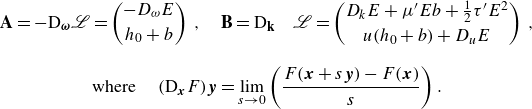 \begin{equation} \begin{gathered} \textbf{A} = -\textrm {D}_{\boldsymbol{\omega }}{\mathscr{L}} = \begin{pmatrix} -D_\omega E\\[3pt] h_0+b \end{pmatrix}\,, \quad \textbf{B} =\textrm {D}_{\textbf{k}}\quad {\mathscr{L}} = \begin{pmatrix} D_k E+\mu^{\prime} Eb+\frac{1}{2}\tau^{\prime} E^{2}\\[3pt] u(h_0+b)+D_u E \end{pmatrix}\,, \\[8pt] \textrm {where } \quad (\textrm {D}_{\boldsymbol{x}}F)\boldsymbol{y} = \lim _{s\to 0} \left(\frac {F(\boldsymbol{x}+s\boldsymbol{y})-F(\boldsymbol{ x})}{s} \right). \end{gathered} \end{equation}
To compute characteristics, we will need the linearisation of (2.16). Differentiating (2.16) with respect to $\boldsymbol{\Omega }$
and
$\boldsymbol{\Omega }$
and $\textbf{K}$
, linearising and introducing the characteristic form
$\textbf{K}$
, linearising and introducing the characteristic form
 \begin{align} \boldsymbol{\Omega }(X,T) = \widehat {\boldsymbol{\Omega }}\textrm {e}^{\texttt {i}(X+cT)}\quad \mbox{and}\quad \textbf{K}(X,T) = \widehat {\textbf{K}}\textrm {e}^{\texttt {i}(X+cT)} \end{align}
results in an eigenvalue problem for the characteristics $c$
:
$c$
:
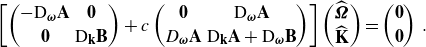 \begin{equation} \left [ \begin{pmatrix} -\textrm {D}_{\boldsymbol{\omega }}\textbf{A} & \textbf{0} \\[2pt] \textbf{0} & \textrm {D}_{\textbf{k}}\textbf{B} \end{pmatrix} +c \begin{pmatrix} \textbf{0} & \textrm {D}_{\boldsymbol{\omega }}\textbf{A} \\[2pt] D_{\boldsymbol{\omega }}\textbf{A} & \textrm {D}_{\textbf{k}}\textbf{A}+\textrm {D}_{\boldsymbol{\omega }}\textbf{B} \end{pmatrix}\right ] \begin{pmatrix} \widehat {\boldsymbol{\Omega }}\\[2pt] \widehat {\textbf{K}}\end{pmatrix} = \begin{pmatrix} \textbf{0}\\[2pt] \textbf{0}\end{pmatrix}\,. \end{equation}
This equation is an example of the general form of the equation for characteristics in multiphase Whitham modulation theory (cf. equation (1.18) in Bridges & Ratliff (Reference Bridges and Ratliff2021)). It is assumed in this construction that $D_{\boldsymbol{\omega }}\textbf{A}$
is invertible, and the first equation in (2.20) has been multiplied by this matrix.
$D_{\boldsymbol{\omega }}\textbf{A}$
is invertible, and the first equation in (2.20) has been multiplied by this matrix.
Combining the two equations in (2.20) by eliminating $\widehat {\boldsymbol{\Omega }}$
, and defining
$\widehat {\boldsymbol{\Omega }}$
, and defining $\boldsymbol{\zeta }=\widehat {\textbf{K}}$
, reduces this equation to the matrix pencil:
$\boldsymbol{\zeta }=\widehat {\textbf{K}}$
, reduces this equation to the matrix pencil:
 \begin{equation} \textbf{E}(c)\boldsymbol{\zeta } = 0\,,\quad \boldsymbol{\zeta } = \begin{pmatrix}\zeta _1\\ \zeta _2\end{pmatrix}\,. \end{equation}
The roots of $\textrm {det}(\textbf{E}(c))=0$
are the characteristics of the modulation equations for the Stokes wave mean-flow interaction. The general form of the
$\textrm {det}(\textbf{E}(c))=0$
are the characteristics of the modulation equations for the Stokes wave mean-flow interaction. The general form of the $2\times 2$
matrix
$2\times 2$
matrix $E(c)$
is
$E(c)$
is
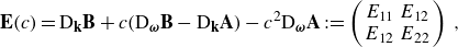 \begin{align} \textbf{E}(c) = \textrm {D}_{\textbf{k}}\textbf{B}+c(\textrm {D}_{\boldsymbol{\omega }}\textbf{B}-\textrm {D}_{\textbf{k}}\textbf{A})-c^{2}\textrm {D}_{\boldsymbol{\omega }}\textbf{A} := \left (\begin{array}{cc} E_{11} & E_{12}\\ E_{12}&E_{22} \end{array}\right )\,, \end{align}
and explicit expressions for the entries $E_{11},E_{12}$
and
$E_{11},E_{12}$
and $E_{22}$
for the water-wave problem are given in Appendix B.
$E_{22}$
for the water-wave problem are given in Appendix B.
From this pencil, we find the characteristic polynomial for the Stokes wave mean-flow modulation is
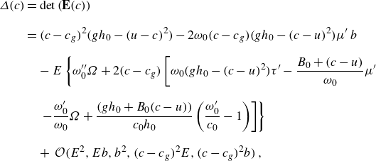 \begin{align} \varDelta (c) & = \textrm {det}\left ( \textbf{E}(c)\right ) \nonumber\\[8pt] & = (c-c_g)^{2}\big(gh_0-(u-c)^{2}\big)-2\omega _0(c-c_g) \big(gh_0-(c-u)^{2}\big)\mu^{\prime}\, b \nonumber\\[8pt] & \quad -E \left \lbrace \omega^{\prime\prime}_0\Omega +2(c-c_g) \left [\omega _0(gh_0-(c-u)^{2})\tau^{\prime}-\frac {B_0+(c-u)}{\omega _0}\mu^{\prime}\right . \right . \nonumber\\[8pt] & \quad \left .\left .-\frac {\omega^{\prime}_0}{\omega _0}\Omega +\frac {\left (g h_0+ B_0(c-u)\right )}{c_0h_0} \left(\frac {\omega^{\prime}_0}{c_0}-1\right)\right ]\right \rbrace \nonumber\\[8pt] & \quad +\, {\mathcal{O}}\big(E^{2},Eb,b^{2},(c-c_{g})^{2}E,(c-c_{g})^{2}b\big)\,, \end{align}
where
 \begin{equation} \Omega (c;k,u) = \omega _2^0\big(gh_0-(c-u)^{2}\big)-\frac {k}{c_0 h_0}\big(B_0^{2}+2B_0(c-u)+gh_0\big)\,. \end{equation}
This polynomial has four roots, admitting four characteristics, and we will find explicit expressions for them in the small amplitude limit $E\ll 1$
. Two of these characteristics are associated with the group velocity of the wave, whereas the final two are related to the linear long-wave speeds. It is the former that we are interested in, as these are the ones which correspond to the Benjamin–Feir instability. The two characteristics of (2.23) that are associated with the group velocity, for small amplitude, are found to be
$E\ll 1$
. Two of these characteristics are associated with the group velocity of the wave, whereas the final two are related to the linear long-wave speeds. It is the former that we are interested in, as these are the ones which correspond to the Benjamin–Feir instability. The two characteristics of (2.23) that are associated with the group velocity, for small amplitude, are found to be
 \begin{equation} c = u+\omega^{\prime}_0 \pm \sqrt {\omega^{\prime\prime}_0 \omega _2^{\textit{eff}}E}+C_2E+\omega _0\mu^{\prime} b +{\mathcal{O}}\big(E^{3/2},Eb,b^{2}\big), \end{equation}
where
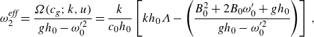 \begin{align} \omega _2^{\textit{eff}} =\frac {\Omega (c_g;k,u)}{gh_0-\omega _0^{\prime 2}} = \frac {k}{c_0 h_0}\left [k h_0 \Lambda -\left (\frac {B_0^{2}+2B_0 \omega^{\prime}_0 +g h_0}{g h_0 -\omega _0^{\prime 2}} \right )\right ]\,, \end{align}
and we have defined for brevity
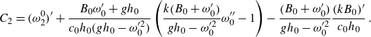 \begin{align} C_2 &= \big(\omega _2^0\big)^{\prime} +\frac {B_0\omega^{\prime}_0+gh_0}{c_0h_0\big(gh_0-\omega _0^{\prime 2}\big)}\left (\frac {k\big(B_0+\omega^{\prime}_0\big)}{gh_0-\omega _0^{\prime 2}} \omega^{\prime\prime}_0-1\right )-\frac {\big(B_0+\omega^{\prime}_0\big)}{gh_0-\omega _0^{\prime 2}}\frac {(kB_0)^{\prime}}{c_0h_0}\,. \end{align}
This expression for $\omega _2^{\textit{eff}}$
is what is called
$\omega _2^{\textit{eff}}$
is what is called $\Omega _2(k)$
in § 16.11 in Whitham (Reference Whitham2011). However, the way it has emerged in this analysis is surprising, as the assumptions are different. In Whitham’s analysis, one must either identify several terms in the analysis and modulation equations to neglect on consistency or size arguments (as in Whitham (Reference Whitham1967)) or appeal to the flux induced by the waves via an argument proposed by Longuet-Higgins in order to arrive at the correct frequency expression (as done in Whitham (Reference Whitham2011)), which essentially constrains the mean induced by the waves
$\Omega _2(k)$
in § 16.11 in Whitham (Reference Whitham2011). However, the way it has emerged in this analysis is surprising, as the assumptions are different. In Whitham’s analysis, one must either identify several terms in the analysis and modulation equations to neglect on consistency or size arguments (as in Whitham (Reference Whitham1967)) or appeal to the flux induced by the waves via an argument proposed by Longuet-Higgins in order to arrive at the correct frequency expression (as done in Whitham (Reference Whitham2011)), which essentially constrains the mean induced by the waves $b$
to be related to the energy density
$b$
to be related to the energy density $E$
. The relative equilibrium approach here, which maintains the independence of
$E$
. The relative equilibrium approach here, which maintains the independence of $b$
and
$b$
and $E$
, does not require this additional information and suggests that the result in Whitham is in fact a consequence of the symmetries of the Lagrangian and thus inherent to the problem itself.
$E$
, does not require this additional information and suggests that the result in Whitham is in fact a consequence of the symmetries of the Lagrangian and thus inherent to the problem itself.
We also need the eigenvector of $\textbf{E}(c)$
when
$\textbf{E}(c)$
when $c$
is a characteristic, in the asymptotic limit
$c$
is a characteristic, in the asymptotic limit $E\to 0$
. In the neighbourhood of the double characteristic, the unfolding of the critical point is of
$E\to 0$
. In the neighbourhood of the double characteristic, the unfolding of the critical point is of ${\mathcal{O}} ({E^{1/2}})$
. In the equation
${\mathcal{O}} ({E^{1/2}})$
. In the equation $\textbf{E}(c){\boldsymbol{\zeta }}=0$
the characteristic (2.25) is substituted in for
$\textbf{E}(c){\boldsymbol{\zeta }}=0$
the characteristic (2.25) is substituted in for $c$
and
$c$
and $\boldsymbol{\zeta }$
is expanded in powers of
$\boldsymbol{\zeta }$
is expanded in powers of $E^{1/2}$
. The details of this expansion can be found in (B2) of Appendix B. Evaluating this eigenvector at the Benjamin–Feir transition
$E^{1/2}$
. The details of this expansion can be found in (B2) of Appendix B. Evaluating this eigenvector at the Benjamin–Feir transition $kh_0 1.363$
, it becomes
$kh_0 1.363$
, it becomes
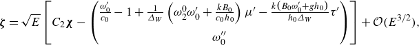 \begin{align} {\boldsymbol{\zeta }}=\sqrt {E}\left [C_2{\boldsymbol{\chi }}-\begin{pmatrix} \frac {\omega^{\prime}_0}{c_0}-1+\frac {1}{\varDelta_W}\left (\omega _2^0\omega^{\prime}_0+\frac {kB_0}{c_0h_0}\right )\mu ^{\prime}-\frac {k\big(B_0\omega^{\prime}_0 + gh_0\big)}{h_0\varDelta_W}\tau ^{\prime}\\[10pt] \omega^{\prime\prime}_0 \end{pmatrix} \right ]+ {\mathcal{O}}\big(E^{3/2}\big), \end{align}
with
 \begin{align} {\boldsymbol{\chi }} = -\frac {1}{c_0h_0\varDelta_W} \begin{pmatrix} gh_0+B_0\omega^{\prime}_0\\[5pt] 0 \end{pmatrix}\,. \end{align}
This eigenvector evaluated at the transition value simplifies to
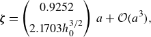 \begin{align} {\boldsymbol{\zeta }} = \begin{pmatrix} 0.9252 \\[4pt] 2.1703h_0^{3/2} \end{pmatrix}\, a + {\mathcal{O}}(a^{3}), \end{align}
since $E=({1}/{2}) g a^{2}$
.
$E=({1}/{2}) g a^{2}$
.
2.2. Bloch spectrum
As can be see from (1.1) and (1.5), a key component of the phase dynamical construction associated with the coefficient of dispersion in the problem is the Bloch spectrum $\sigma (\nu )$
, with
$\sigma (\nu )$
, with $\nu$
the spatial Floquet exponent/Bloch wavenumber, for the Stokes wave solution. The Bloch spectrum consists of the eigenvalues of the linearisation of the full water-wave problem about the Stokes wave and has a central place in understanding the stability of Stokes waves in finite depth (Deconinck & Oliveras Reference Deconinck and Oliveras2011; Berti et al. Reference Berti, Maspero and Ventura2023; Creedon & Deconinck Reference Creedon and Deconinck2023; Berti et al. Reference Berti, Maspero and Ventura2024), and so it is unsurprising that it features as a component of the phase dynamics reduction. In this paper only third-order dispersive effects are required in the asymptotic analysis because only the third-order Taylor coefficient of the Bloch spectrum about the zero Bloch wavenumber is required. In this section we identify an appropriate choice for the Bloch spectrum that is both analytically tractable and representative of the problem.
$\nu$
the spatial Floquet exponent/Bloch wavenumber, for the Stokes wave solution. The Bloch spectrum consists of the eigenvalues of the linearisation of the full water-wave problem about the Stokes wave and has a central place in understanding the stability of Stokes waves in finite depth (Deconinck & Oliveras Reference Deconinck and Oliveras2011; Berti et al. Reference Berti, Maspero and Ventura2023; Creedon & Deconinck Reference Creedon and Deconinck2023; Berti et al. Reference Berti, Maspero and Ventura2024), and so it is unsurprising that it features as a component of the phase dynamics reduction. In this paper only third-order dispersive effects are required in the asymptotic analysis because only the third-order Taylor coefficient of the Bloch spectrum about the zero Bloch wavenumber is required. In this section we identify an appropriate choice for the Bloch spectrum that is both analytically tractable and representative of the problem.
Due to the low-amplitude nature of the Stokes waves within this paper, it would be fair to expect the spectrum that arises from such problems to be akin to the spectrum of nonlinear Schrödinger-type models:
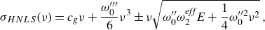 \begin{equation} \sigma _{HNLS}(\nu ) =c_g \nu + \frac {\omega^{\prime\prime\prime}_0}{6}\nu ^{3} \pm \nu \sqrt {\omega^{\prime\prime}_0\omega _2^{\textit{eff}}E+\frac {1}{4}\omega _0^{\prime \prime 2}\nu ^{2}}\,, \end{equation}
where the subscript $HNLS$
indicates that this is the exact spectrum for the nonlinear Schrödinger equation with higher-order dispersion terms (Ratliff Reference Ratliff2021). To leading order in
$HNLS$
indicates that this is the exact spectrum for the nonlinear Schrödinger equation with higher-order dispersion terms (Ratliff Reference Ratliff2021). To leading order in $E$
and without higher-order dispersive effects, this expansion has been shown the same in the full water-wave problem in the vicinity of the Benjamin–Feir instability (Bridges & Mielke Reference Bridges and Mielke1995). However, the mean-flow effects in nonlinear Schrödinger models are treated adiabatically and as such may not be captured fully in this Bloch spectrum. To remedy this we compare this nonlinear Schrödinger Bloch spectrum with a model where the mean flow is non-adiabatic, which within this paper is the one obtained from the Benney–Roskes equation, given by (Benney & Roskes Reference Benney and Roskes1969)
$E$
and without higher-order dispersive effects, this expansion has been shown the same in the full water-wave problem in the vicinity of the Benjamin–Feir instability (Bridges & Mielke Reference Bridges and Mielke1995). However, the mean-flow effects in nonlinear Schrödinger models are treated adiabatically and as such may not be captured fully in this Bloch spectrum. To remedy this we compare this nonlinear Schrödinger Bloch spectrum with a model where the mean flow is non-adiabatic, which within this paper is the one obtained from the Benney–Roskes equation, given by (Benney & Roskes Reference Benney and Roskes1969)
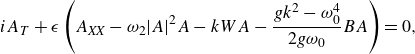 \begin{gather} iA_T+\epsilon \left (A_{\textit{XX}}-\omega _2|A|^{2}A-k WA-\frac {gk^{2}-\omega _0^4}{2g\omega _0}BA\right ) = 0, \end{gather}
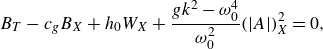 \begin{gather} B_T-c_gB_X+h_0W_X+\frac {gk^{2}-\omega _0^4}{\omega _0^{2}}(|A|)_X^{2} = 0, \end{gather}
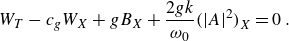 \begin{gather} W_T-c_gW_X+gB_X+\frac {2gk}{\omega _0}\big(|A|^{2}\big)_X = 0\,. \end{gather}
In this equation, $A$
is the complex amplitude of the wave,
$A$
is the complex amplitude of the wave, $B$
is the mean level variation and
$B$
is the mean level variation and $W$
is the mean velocity. The small parameter
$W$
is the mean velocity. The small parameter $\epsilon$
(which differs from
$\epsilon$
(which differs from $\varepsilon$
in the modulation theory) gives the order of magnitude of the wave amplitude. It is equivalent to the smallness of the parameter
$\varepsilon$
in the modulation theory) gives the order of magnitude of the wave amplitude. It is equivalent to the smallness of the parameter $a$
and thus allows one to relate the Bloch spectrum of the Benney–Roskes system to the modulation theory of this paper. Whilst the full closed-form expression for the spectrum is complicated, we only require its long-wave expansion, which in terms of the Stokes wave parameters reads
$a$
and thus allows one to relate the Bloch spectrum of the Benney–Roskes system to the modulation theory of this paper. Whilst the full closed-form expression for the spectrum is complicated, we only require its long-wave expansion, which in terms of the Stokes wave parameters reads
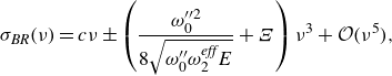 \begin{align} \sigma _{\textit{BR}}(\nu ) = c \nu \pm \left (\frac {\omega _0^{\prime \prime 2}}{8 \sqrt {\omega^{\prime\prime}_0 \omega _2^{\textit{eff}}E}}+\Xi \right ) \nu ^{3} +{\mathcal{O}}(\nu ^5), \end{align}
where the characteristic $c$
is defined as in (2.25) and
$c$
is defined as in (2.25) and
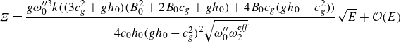 \begin{align} \Xi = \frac {g\omega _0^{\prime \prime 3}k\big(\big(3c_g^{2} + g h_0\big)\big(B_0^{2} + 2 B_0c_g + g h_0\big) + 4 B_0 c_g \big(gh_0-c_g^{2}\big)\big)}{4c_0h_0\big(gh_0-c_g^{2}\big)^{2}\sqrt {\omega^{\prime\prime}_0\omega _2^{\textit{eff}}}}\sqrt {E}+ {\mathcal{O}}(E) \end{align}
characterises the additional dispersive effects due to the mean flow. We note that this spectrum only differs from the long-wave expansion of the classical nonlinear Schrödinger equation at ${\mathcal{O}}(\sqrt {E})$
, but does not alter the Benjamin–Feir instability boundary. As such, we postulate that we may augment the above spectrum with the third-order dispersive term in (2.31). (Formally, this can be done by following asymptotic procedures such as in Slunyaev (Reference Slunyaev2005) or Kakutani & Michihiro (Reference Kakutani and Michihiro1983), noting that the mean-flow effects on the stability have already been accounted for.) This gives the Bloch spectrum that we utilise within this paper:
${\mathcal{O}}(\sqrt {E})$
, but does not alter the Benjamin–Feir instability boundary. As such, we postulate that we may augment the above spectrum with the third-order dispersive term in (2.31). (Formally, this can be done by following asymptotic procedures such as in Slunyaev (Reference Slunyaev2005) or Kakutani & Michihiro (Reference Kakutani and Michihiro1983), noting that the mean-flow effects on the stability have already been accounted for.) This gives the Bloch spectrum that we utilise within this paper:
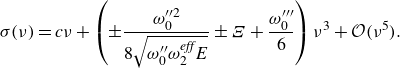 \begin{equation} \sigma (\nu ) = c \nu +\left (\pm \frac {\omega _0^{\prime \prime 2}}{8 \sqrt {\omega^{\prime\prime}_0 \omega _2^{\textit{eff}}E}} \pm \Xi +\frac {\omega^{\prime\prime\prime}_0}{6}\right ) \nu ^{3}+ {\mathcal{O}}(\nu ^5). \end{equation}
3. Phase modulation in the hyperbolic region
The hyperbolic region is the region in which Stokes waves coupled to mean flow exist and the Whitham modulation equations, linearised about the Stokes wave (2.20), have four real characteristics. Everywhere in this region the modulation can be re-scaled as in (1.2) to derive the KdV equation (1.5). This KdV equation is in a characteristic moving frame with the speed determined by a characteristic from the generic Whitham theory. The theory for this re-modulation follows Ratliff & Bridges (Reference Ratliff and Bridges2016a
) and Ratliff (Reference Ratliff2019, Reference Ratliff2021). The form for the re-modulation is (1.2) with $\alpha =1$
and
$\alpha =1$
and $\beta =3$
. The velocity potential and free surface are expressed as
$\beta =3$
. The velocity potential and free surface are expressed as
 \begin{align} Z(x,y,t) = \widehat {Z}\big({\boldsymbol{\theta }}+\varepsilon {\boldsymbol{\Theta }}(X,T);\textbf{k}+\varepsilon ^{2}\textbf{K}(X,T),\boldsymbol{\omega } + \varepsilon ^{2} c\textbf{K} +\varepsilon ^{3}\boldsymbol{\Omega }\big) +\varepsilon ^4 W(X,T,\varepsilon ), \end{align}
where $Z(x,y,t)=(\phi (x,y,t),\eta (x,t))$
,
$Z(x,y,t)=(\phi (x,y,t),\eta (x,t))$
, $\widehat {Z}({\boldsymbol{\theta }};\textbf{k},\boldsymbol{\omega })$
is the Stokes wave plus mean flow and
$\widehat {Z}({\boldsymbol{\theta }};\textbf{k},\boldsymbol{\omega })$
is the Stokes wave plus mean flow and $c$
is one of the wave characteristics in the hyperbolic region:
$c$
is one of the wave characteristics in the hyperbolic region:
 \begin{equation} c = c_g \pm \sqrt {\omega^{\prime\prime}_0(k_0) \omega _2^{\textit{eff}}(k_0)} a+\cdots \quad \mbox{with } \quad \omega^{\prime\prime}_0(k_0) \omega _2^{\textit{eff}}(k_0)\gt 0\,. \end{equation}
The modulation equations are then obtained by substitution of the above Stokes wave solution with these perturbed wave quantities into the water-wave equations and solving the resulting system at each order of the small parameter $\varepsilon$
. The strategy is given in Ratliff & Bridges (Reference Ratliff and Bridges2016a
) and Ratliff (Reference Ratliff2019) and so we skip details. The resulting KdV equation has the form given in (1.5), which we repeat here as we evaluate the key coefficients:
$\varepsilon$
. The strategy is given in Ratliff & Bridges (Reference Ratliff and Bridges2016a
) and Ratliff (Reference Ratliff2019) and so we skip details. The resulting KdV equation has the form given in (1.5), which we repeat here as we evaluate the key coefficients:
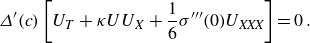 \begin{equation} \varDelta^{\prime}(c) \left [U_T+\kappa UU_X+\frac {1}{6}\sigma^{\prime\prime\prime}(0)U_{\textit{XXX}}\right ] = 0\,. \end{equation}
The function $U(X,T)$
in (3.3) is obtained by projection of
$U(X,T)$
in (3.3) is obtained by projection of $\textbf{K}(X,T)$
in the direction of the eigenvector
$\textbf{K}(X,T)$
in the direction of the eigenvector ${\boldsymbol{\zeta }}$
of
${\boldsymbol{\zeta }}$
of $\textbf{E}(c){\boldsymbol{\zeta }}=0$
with
$\textbf{E}(c){\boldsymbol{\zeta }}=0$
with $\textbf{E}(c)$
defined in (2.21) with its argument evaluated at (3.2):
$\textbf{E}(c)$
defined in (2.21) with its argument evaluated at (3.2):
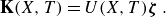 \begin{equation} \textbf{K}(X,T) = U(X,T){\boldsymbol{\zeta }}\,. \end{equation}
It is important to note that this KdV equation is not the classical KdV equation in shallow water, which can also be derived using phase dynamics (Bridges Reference Bridges2014), but the coefficients and implications are different. This is because in addition to perturbing the mean-free-surface level and horizontal velocity that the classical KdV would suggest, it additionally alters the wavenumber, frequency and amplitude of the surface Stokes wavetrain with non-zero amplitude. Indeed, the solitary wave solution of (1.5) is in fact a dark solitary wave (bi-asymptotic to a Stokes travelling wave). Hence the hyperbolic region is not only filled with modulationally stable Stokes waves, it is also filled with dark solitary waves, each moving at its local characteristic speed (3.2).
The coefficient $\varDelta (c)$
is defined in (2.23), and its derivative is found to be
$\varDelta (c)$
is defined in (2.23), and its derivative is found to be
 \begin{equation} \varDelta^{\prime}(c) = \pm 2\big(g h_0-\omega _0^{\prime 2}\big)\sqrt {\omega^{\prime\prime}_0 \omega _2^{\textit{eff}}E}+ {\mathcal{O}}\big(E^{3/2}\big). \end{equation}
The second important term is the dispersive term $\sigma^{\prime\prime\prime}(0)$
in the KdV equation, which is obtained from the Bloch spectrum. The Bloch spectrum is the temporal eigenvalue
$\sigma^{\prime\prime\prime}(0)$
in the KdV equation, which is obtained from the Bloch spectrum. The Bloch spectrum is the temporal eigenvalue $\sigma (\nu )$
of the linearisation of the full equations considered as a function of the spatial Floquet exponent (see also § 2.2). Using the spectrum (2.37), we can readily obtain
$\sigma (\nu )$
of the linearisation of the full equations considered as a function of the spatial Floquet exponent (see also § 2.2). Using the spectrum (2.37), we can readily obtain
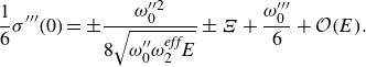 \begin{align} \frac {1}{6} \sigma^{\prime\prime\prime}(0) = \pm \frac {\omega _0^{\prime \prime 2}}{8 \sqrt {\omega^{\prime\prime}_0 \omega _2^{\textit{eff}}E}}\pm \Xi +\frac {\omega^{\prime\prime\prime}_0}{6}+ {\mathcal{O}}(E). \end{align}
Note that although this expression appears to be singular at the Benjamin–Feir transition $\omega^{\prime\prime}_0\omega _2^{\textit{eff}} = 0$
the singularity is of the same order as the zero of
$\omega^{\prime\prime}_0\omega _2^{\textit{eff}} = 0$
the singularity is of the same order as the zero of $\varDelta^{\prime}(c)$
at this point, meaning the dispersive term in the KdV equation is finite and non-zero at this transition.
$\varDelta^{\prime}(c)$
at this point, meaning the dispersive term in the KdV equation is finite and non-zero at this transition.
The third coefficient of interest is the coefficient $\kappa$
of the nonlinearity:
$\kappa$
of the nonlinearity:
 \begin{align} \kappa = \begin{pmatrix} \textrm {D}_{\textbf{k}} c(\textbf{k},\boldsymbol{\omega })\\[2pt] \textrm {D}_{\boldsymbol{\omega }} c(\textbf{k},\boldsymbol{\omega }) \end{pmatrix} \cdot \begin{pmatrix} {\boldsymbol{\zeta }}\\[2pt] c {\boldsymbol{\zeta }} \end{pmatrix}\,. \end{align}
This latter expression is related to the concept of genuine nonlinearity of the Whitham modulation equations, in the sense of Lax (cf. Lax Reference Lax1973; Ratliff Reference Ratliff2021). Evaluation of this coefficient for the water-wave problem is straightforward but lengthy. Using the expressions (2.25) and (B2) we can show that
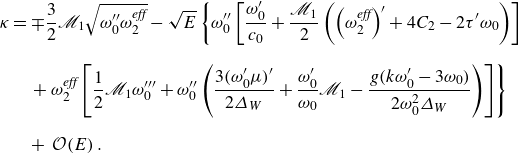 \begin{align} \kappa &= \mp \frac {3}{2}{\mathscr{M}}_{1}\sqrt {\omega^{\prime\prime}_0 \omega _2^{\textit{eff}}}-\sqrt {E}\left \lbrace \omega^{\prime\prime}_0 \left [\frac {\omega^{\prime}_0}{c_0}+\frac {\mathscr{M}_{1}}{2}\left (\left(\omega _2^{\textit{eff}}\right)^{\prime}+4C_2-2\tau^{\prime}\omega _0\right )\right ]\right . \nonumber\\[8pt] & \quad \left . +\, \omega _2^{\textit{eff}}\left [\frac{1}{2}{\mathscr{M}}_{1}\omega^{\prime\prime\prime}_0 +\omega^{\prime\prime}_0\left (\frac {3(\omega^{\prime}_0\mu )^{\prime}}{2\varDelta_W}+\frac {\omega^{\prime}_0}{\omega _0}{\mathscr{M}}_{1}-\frac {g(k\omega^{\prime}_0-3\omega _0)}{2\omega _0^2\varDelta_W}\right )\right ]\right \rbrace \nonumber\\[8pt] &\quad +\, \mathcal{O}(E)\,.\end{align}
The coefficient ${\mathscr{M}_{1}}$
is given in equation (A2) of Appendix A where it is associated with the change of wave properties due to mean velocity changes. The coefficient of the nonlinearity
${\mathscr{M}_{1}}$
is given in equation (A2) of Appendix A where it is associated with the change of wave properties due to mean velocity changes. The coefficient of the nonlinearity $\kappa$
is finite at the Benjamin–Feir transition, and so once multiplied by (3.5) the quadratic term in the KdV equation will vanish. This is important at the Benjamin–Feir transition, and is the reason that the nonlinearity within the phase dynamical description goes from purely quadratic as in (1.5) to involving the cubic and mixed quadratic terms seen in (1.1).
$\kappa$
is finite at the Benjamin–Feir transition, and so once multiplied by (3.5) the quadratic term in the KdV equation will vanish. This is important at the Benjamin–Feir transition, and is the reason that the nonlinearity within the phase dynamical description goes from purely quadratic as in (1.5) to involving the cubic and mixed quadratic terms seen in (1.1).
In summary, in the Benjamin–Feir stable region, the KdV equation which emerges, for the faster of the two characteristic speeds, is
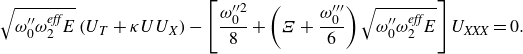 \begin{equation} \sqrt {\omega^{\prime\prime}_0 \omega _2^{\textit{eff}}E}\,(U_T+\kappa UU_X)-\left [\frac {\omega _0^{\prime \prime 2}}{8}+\left (\Xi +\frac {\omega^{\prime\prime\prime}_0}{6}\right )\sqrt {\omega^{\prime\prime}_0 \omega _2^{\textit{eff}} E}\right ]U_{\textit{XXX}} = 0. \end{equation}
This KdV equation is asymptotically correct to order $E$
. However the KdV equation does not support heteroclinic connections, thereby precluding jumps in frequency and wavenumber. This is known for two reasons. The first is by considering solutions of permanent form. By utilising the Hamiltonian structure of the KdV equation, one finds the heteroclinic connection of permanent form must satisfy
$E$
. However the KdV equation does not support heteroclinic connections, thereby precluding jumps in frequency and wavenumber. This is known for two reasons. The first is by considering solutions of permanent form. By utilising the Hamiltonian structure of the KdV equation, one finds the heteroclinic connection of permanent form must satisfy
 \begin{align} \alpha U_{\xi }^{2}+\beta U^{3}-VU^{2}+IU \equiv \alpha U_{\xi }^{2}+ {\mathcal{V}}(U) = 0 \end{align}
for coefficients $\alpha ,\,\beta$
, wave speed
$\alpha ,\,\beta$
, wave speed $V$
, travelling coordinate
$V$
, travelling coordinate $\xi =X-VT$
and integration constant
$\xi =X-VT$
and integration constant $I$
. Unlike heteroclinic connections (which require one simple and one repeated root), heteroclinic connections require two saddle notes to exist in the above dynamical system, equivalent to
$I$
. Unlike heteroclinic connections (which require one simple and one repeated root), heteroclinic connections require two saddle notes to exist in the above dynamical system, equivalent to ${\mathcal{V}}$
possessing two double roots (Kamchatnov et al. Reference Kamchatnov, Kuo, Lin, Horng, Gou, Clift, El and Grimshaw2012), which is impossible for a cubic polynomial. Any step-like solution that is not of permanent form is known to disintegrate into a train of solitary waves in the long-time limit (Hruslov Reference Hruslov1976; Venakides Reference Venakides1986). Hence, in the strictly hyperbolic (modulationally stable) regime there cannot be a permanent change in wavenumber.
${\mathcal{V}}$
possessing two double roots (Kamchatnov et al. Reference Kamchatnov, Kuo, Lin, Horng, Gou, Clift, El and Grimshaw2012), which is impossible for a cubic polynomial. Any step-like solution that is not of permanent form is known to disintegrate into a train of solitary waves in the long-time limit (Hruslov Reference Hruslov1976; Venakides Reference Venakides1986). Hence, in the strictly hyperbolic (modulationally stable) regime there cannot be a permanent change in wavenumber.
As noted above, it is apparent from the expressions for the coefficients that the first two terms of this KdV equation are zero whenever $\omega _2^{\textit{eff}} = 0$
, occurring exactly at the Benjamin–Feir transition, which signifies a change in scale. This inevitably leads to at least cubic nonlinearities emerging, although quadratic nonlinearities of mixed type (i.e. involving spatial and temporal derivatives) are a priori also anticipated. This theory is developed in the next section, resulting in a modified version of the two-way Boussinesq equation. This new modulation equation will have the necessary nonlinearities and dispersion to support a heteroclinic connection that will lead to downshifting of the Stokes waves.
$\omega _2^{\textit{eff}} = 0$
, occurring exactly at the Benjamin–Feir transition, which signifies a change in scale. This inevitably leads to at least cubic nonlinearities emerging, although quadratic nonlinearities of mixed type (i.e. involving spatial and temporal derivatives) are a priori also anticipated. This theory is developed in the next section, resulting in a modified version of the two-way Boussinesq equation. This new modulation equation will have the necessary nonlinearities and dispersion to support a heteroclinic connection that will lead to downshifting of the Stokes waves.
4. Phase modulation near the Benjamin–Feir transition
In approaching the Benjamin–Feir transition, two singularities arise. Firstly, two characteristics coalesce as noted in § 2 and secondly, the coefficient of the quadratic nonlinearity vanishes as noted in § 3. In light of this we utilise time scaling typically used to derive two-way Boussinesq equations, used to rebalance the time portion of the dynamics (Ratliff & Bridges Reference Ratliff and Bridges2016b
), in tandem with scalings used to obtain the modified KdV equation where cubic terms resolve vanishing quadratic nonlinearities (Gear & Grimshaw Reference Gear and Grimshaw1983; Ratliff Reference Ratliff2021). Therefore, in the re-modulation the coalescing characteristics change in light of the above observations, the first resulting in the small time exponent changing from $\beta =3$
to
$\beta =3$
to $\beta =2$
and the second a change of perturbation scales from
$\beta =2$
and the second a change of perturbation scales from $\alpha = 1$
to
$\alpha = 1$
to $\alpha = 0$
. With the loss of quadratic nonlinearity and emergence of cubic nonlinearity new terms appear in the equation as shown in (1.1) rewritten here in a different form:
$\alpha = 0$
. With the loss of quadratic nonlinearity and emergence of cubic nonlinearity new terms appear in the equation as shown in (1.1) rewritten here in a different form:
 \begin{equation} \alpha _1U_{\textit{TT}} + \big(\alpha _2U^{3} + \alpha _4 U_{\textit{XX}}\big)_{\textit{XX}} +\alpha _3\big(2UU_T+U_X\partial _X^{-1}U_T\big)_X =0\,. \end{equation}
The first three terms are the two-way Boussinesq equation with a cubic nonlinearity. The latter term, multiplied by $\alpha _3$
, is required to balance the cubic nonlinearity. With
$\alpha _3$
, is required to balance the cubic nonlinearity. With $U$
of order
$U$
of order $\varepsilon$
,
$\varepsilon$
, $X$
of order
$X$
of order $\varepsilon$
and
$\varepsilon$
and $T$
of order
$T$
of order $\varepsilon ^{2}$
, the three nonlinear terms are in balance:
$\varepsilon ^{2}$
, the three nonlinear terms are in balance:
 \begin{align} \big(U^{3}\big)_{\textit{XX}} \sim \varepsilon ^5\,,\quad (UU_T)_X \sim \varepsilon ^5\quad \mbox{and } \quad \big(U_X\partial _X^{-1}U_T\big)_X \sim \varepsilon ^5. \end{align}
A detailed derivation of this equation is given in § 4.5.3 of Ratliff (Reference Ratliff2017) for the case of the laboratory frame, but can be extended to the case of the characteristic moving frame using recent works by the authors (most notably, Bridges & Ratliff Reference Bridges and Ratliff2017; Ratliff Reference Ratliff2021). The dependent variable $U$
is again obtained as a projection of the wavenumber onto the eigenvector,
$U$
is again obtained as a projection of the wavenumber onto the eigenvector, $\textbf{K}=U{\boldsymbol{\zeta }}$
, as in (3.4), although here the eigenvector is that associated with coalesced characteristics.
$\textbf{K}=U{\boldsymbol{\zeta }}$
, as in (3.4), although here the eigenvector is that associated with coalesced characteristics.
General expressions for the parameters in (4.1) are given in terms of the averaged Lagrangian in equation (4.27) of Ratliff (Reference Ratliff2017); however, the more accessible way to compute this number is to use the connection of the coefficients to the Bloch spectrum and expansions of the flux vector as in Ratliff (Reference Ratliff2021). The evaluations of the coefficients for the water-wave problem at the Benjamin–Feir transition are lengthy, and results are summarised here. The dispersion coefficient is
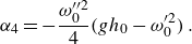 \begin{align} \alpha _4 = -\frac {\omega _0^{\prime \prime 2}}{4}\big(gh_0-\omega _0^{\prime 2}\big)\,. \end{align}
The time derivative term, which goes from a first-order derivative to a second-order derivative at the Benjamin–Feir transition, has coefficient
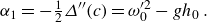 \begin{align} \alpha _1 = -\tfrac{1}{2}\varDelta^{\prime\prime}(c) = \omega _0^{\prime 2}-gh_0\,. \end{align}
The most complicated coefficient is that multiplying the cubic nonlinearity. Evaluating the formula on the weakly nonlinear Stokes wave gives
 \begin{align} \alpha _2 = \frac{1}{2}\left [\varDelta^{\prime\prime} \kappa ^{2}+\kappa \left [ \begin{pmatrix} \textrm {D}_{\textbf{k}} \varDelta^{\prime}\\ \textrm {D}_{\boldsymbol{\omega }} \varDelta^{\prime} \end{pmatrix} \cdot \begin{pmatrix} {\boldsymbol{\zeta }}\\ c {\boldsymbol{\zeta }} \end{pmatrix}\right ] \right ] = -\frac {\kappa \omega^{\prime\prime}_0}{12\varDelta_W}\left(\left(\omega _2^{\textit{eff}}\right)^{\prime}+4C_2\right)\varDelta^{\prime\prime}\,. \end{align}
At the Benjamin–Feir transition, $\kappa$
reduces to
$\kappa$
reduces to
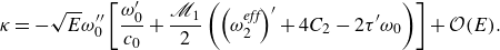 \begin{align} \kappa = -\sqrt {E} \omega^{\prime\prime}_0\left [\frac {\omega^{\prime}_0}{c_0}+\frac {{\mathscr{M}}_{1}}{2}\left (\left(\omega _2^{\textit{eff}}\right)^{\prime}+4C_2-2\tau^{\prime} \omega _0\right )\right ]+{\mathcal{O}}(E). \end{align}
The last coefficient to compute is for the quadratic terms, which emerge due to the simultaneous vanishing of the time and nonlinear terms in the KdV term. This has the coefficient
 \begin{align} \alpha _3 = \varDelta^{\prime\prime} \kappa .\end{align}
Overall, this gives the modified two-way Boussinesq equation as
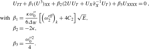 \begin{equation} \begin{array}{rl} &U_{\textit{TT}}+\beta _1(U^{3})_{\textit{XX}}+\beta _2\big(2UU_T+U_X\partial _X^{-1}U_T\big)+\beta _3 U_{\textit{XXXX}} = 0\,,\\[8pt] \textrm {with } &\beta _1 = \dfrac {\kappa \omega^{\prime\prime}_0}{6\varDelta_W}\left [\left(\omega _2^{\textit{eff}}\right)_k+4C_2\right ]\sqrt {E},\\[8pt] &\beta _2 = -2\kappa ,\\[8pt] &\beta _3 = \dfrac {\omega _0^{\prime \prime 2}}{4}. \end{array} \end{equation}
The remaining depth and amplitude effects, to leading order, can be removed with the rescaling
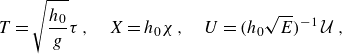 \begin{align} T = \sqrt {\frac {h_0}{g}}\tau \,, \quad X = h_0 \chi \,, \quad U = \big(h_0 \sqrt {E}\big)^{-1}\, {\mathcal{U}}\,, \end{align}
reducing the phase dynamical equation at the Benjamin–Feir transition point to simply
 \begin{equation} {\mathcal{U}}_{\tau \tau }-\left(0.1195{\mathcal{U}}^{3}-0.02247\, {\mathcal{U}}_{\chi \chi }\right)_{\chi \chi }+5.2256 \left(2\,{\mathcal{U}}{\mathcal{U}}_\tau +{\mathcal{U}}_\chi \partial _\chi ^{-1}{\mathcal{U}}_\tau \right)_\chi = 0\,. \end{equation}
It is this equation that we analyse in order to determine the evolution of the wave and mean flow at the Benjamin–Feir transition, and the downshift phenomenon.
4.1. Heteroclinic connections representing frequency downshifting
We now solve (4.10), postulating travelling wave solutions of the form
 \begin{align} {\mathcal{U}}(X,T) = R(\xi )\,,\quad \mbox{with } \quad \xi = X - V T\,, \end{align}
parametrised by $V$
, where
$V$
, where $V$
is the speed of the travelling front. To capture permanent downshifting of the Stokes waves we prescribe the boundary conditions
$V$
is the speed of the travelling front. To capture permanent downshifting of the Stokes waves we prescribe the boundary conditions
 \begin{align} \lim _{\xi \to \infty }R(\xi ) = K_1\,, \quad \lim _{\xi \to -\infty } = K_2\,, \qquad K_2\neq K_1\,. \end{align}
These boundary conditions correspond to a pair of asymptotic wavenumbers for the perturbed Stokes waves of the form $k_{1,2} = k_0+\varepsilon \zeta _1 K_{1,2}$
, connecting initial state
$k_{1,2} = k_0+\varepsilon \zeta _1 K_{1,2}$
, connecting initial state $k_1$
(assuming
$k_1$
(assuming $V\gt 0$
without loss of generality) to
$V\gt 0$
without loss of generality) to $k_2$
. These assumptions transform (4.10) into an ordinary differential equation, which may be integrated to form a system possessing a quartic potential, with the travelling front now represented by a heteroclinic connection.
$k_2$
. These assumptions transform (4.10) into an ordinary differential equation, which may be integrated to form a system possessing a quartic potential, with the travelling front now represented by a heteroclinic connection.
The boundary conditions impose that the quartic potential of the ordinary differential equation must possess two repeated roots at $K_1$
and
$K_1$
and $K_2$
, and so the system for the frequency downshifting solution takes the form
$K_2$
, and so the system for the frequency downshifting solution takes the form
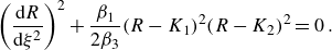 \begin{equation} \left (\frac {{\textrm d}R}{{\textrm d} \xi ^{2}}\right )^{2} +\frac {\beta _1}{2\beta _3}(R-K_1)^{2}(R-K_2)^{2} = 0\,. \end{equation}
A comparison between (4.10) and the above gives that the far-field states take one of the following pairs of values:
 \begin{align} K_{1,2} = \frac {V}{2\beta _1} \left (\beta _2 \pm \sqrt {3\beta _2^{2}-4\beta _1}\right ) = \left (-21.8564 \pm 37.9667\right ) V .\end{align}
The square root exceeding the leading factor ensures the conjugate states lie on opposite sides of the Benjamin–Feir threshold, and thus connect a Stokes wave which is modulationally unstable to one which is modulationally stable. This is a valuable insight, as this suggests that a transition which leads to $K_2\gt K_1$
would be inadmissible owing to the fact that the state it is attempting to connect to is an unstable wavetrain, rather than a uniform wavetrain. Thus, it follows that one should choose
$K_2\gt K_1$
would be inadmissible owing to the fact that the state it is attempting to connect to is an unstable wavetrain, rather than a uniform wavetrain. Thus, it follows that one should choose $K_2\lt 0$
and
$K_2\lt 0$
and $K_1\gt 0$
on physical grounds to avoid such a scenario. There is an alternative reasoning based on energetics that may also be employed, which is described below in § 5.
$K_1\gt 0$
on physical grounds to avoid such a scenario. There is an alternative reasoning based on energetics that may also be employed, which is described below in § 5.
Moreover, a secondary insight is that the speed of this transition between bi-asymptotic states is linked to the size of the wavenumber transition, suggesting that larger deviations from the carrier wave will be resolved much more rapidly, in line with what one would expect experimentally. With these boundary conditions and reasoning, this double root corresponds to the jump profile
 \begin{equation} R(\xi ) = \frac{1}{2} \ \left [K_1+K_2+(K_1-K_2)\tanh (0.7814\,(K_2-K_1)\xi ) \right ]\,. \end{equation}
The solution family presented here affords novel insight into the frequency downshifting phenomenon from a conservative but dispersive point of view. On the other hand, it is useful to discuss its limitations. Primarily, the solution here presents the connection between two bi-asymptotic states but is unlikely to accurately describe the evolution of the wave as it transitions between them. This is due to the fact that a great number of the higher harmonics and their sidebands contribute to the energy transfer within the wavetrain. This is apparent in the original experiments of Lake et al. (Reference Lake, Yuen, Rungaldier and Ferguson1977), where there is a devolution from sideband and harmonic dynamics to a much broader spectral wave evolution.
5. Energetics of frequency downshifting
This analysis of the previous section highlights that two heteroclinic connections are supported by this system, which initially suggests both upshifting and downshifting are permissible. Here we provide some discussion as to how this can be interpreted energetically, leading us to conclude that frequency downshifting arises instead of upshifting. In this discussion, we denote the connection where $k_2\lt k_0$
as the lower sideband solution and
$k_2\lt k_0$
as the lower sideband solution and $k_1\gt k_0$
as the upper sideband. These correspond to the bi-asymptotic states of
$k_1\gt k_0$
as the upper sideband. These correspond to the bi-asymptotic states of $U$
characterised by
$U$
characterised by $K_2\lt 0\lt K_1$
, respectively.
$K_2\lt 0\lt K_1$
, respectively.
We begin our discussion with the energy density of the wave, $E$
, under the action of the jump solution (4.15). By comparing lower and upper sideband wavenumbers we are able to show from (A1) that the energy density of the sidebands is related to the energy density of the carrier wave,
$E$
, under the action of the jump solution (4.15). By comparing lower and upper sideband wavenumbers we are able to show from (A1) that the energy density of the sidebands is related to the energy density of the carrier wave, $E_0$
, to leading order via
$E_0$
, to leading order via
 \begin{align} E_{1,2} = E_0-\varepsilon \sqrt {E}\,\omega^{\prime\prime}_0{\mathscr{M}}_{1}K_{1,2}+{\mathcal{O}}\big(\varepsilon ^{2} \sqrt {E},\varepsilon E\big)\,. \end{align}
Thus, it is clear that $E_1\lt E_0\lt E_2$
and so more energy is passed to the lower sideband than to the upper sideband under the jump mechanism. This is in line with experimental (e.g. Lake et al. Reference Lake, Yuen, Rungaldier and Ferguson1977; Melville Reference Melville1982) and theoretical (e.g. Bryant Reference Bryant1982) observations. The primary driver of this energy exchange is the mean-flow effect, suggesting the mechanism for the sideband asymmetry is indeed a mean-flow aspect of the problem rather than the wave. Additionally, the energy of the lower sideband as
$E_1\lt E_0\lt E_2$
and so more energy is passed to the lower sideband than to the upper sideband under the jump mechanism. This is in line with experimental (e.g. Lake et al. Reference Lake, Yuen, Rungaldier and Ferguson1977; Melville Reference Melville1982) and theoretical (e.g. Bryant Reference Bryant1982) observations. The primary driver of this energy exchange is the mean-flow effect, suggesting the mechanism for the sideband asymmetry is indeed a mean-flow aspect of the problem rather than the wave. Additionally, the energy of the lower sideband as $T\to \infty$
under this mechanism exceeds that of the carrier wave, as also seen in the aforementioned studies. These facts together suggest that there is an overall shift in energy downwards in the spectrum over long time, and thus the spectral peak moves from the carrier wavenumber to that of the lower sideband.
$T\to \infty$
under this mechanism exceeds that of the carrier wave, as also seen in the aforementioned studies. These facts together suggest that there is an overall shift in energy downwards in the spectrum over long time, and thus the spectral peak moves from the carrier wavenumber to that of the lower sideband.
The energy density alone does not, however, indicate whether the upshift or downshift is ultimately selected by the system but can be resolved by looking at the total wave energy. Recall the definition of wave energy for the water-wave problem (Whitham Reference Whitham2011):
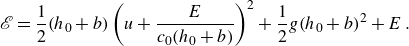 \begin{align} {\mathscr{E}} = \frac{1}{2}(h_0+b)\left (u+\frac {E}{c_0(h_0+b)}\right )^{2}+\frac{1}{2}g (h_0+b)^{2}+E\,. \end{align}
Let us denote the wave energy of the carrier wave by ${\mathscr{E}}_{0}$
. Then to leading order the energy of the upper and lower sidebands is
${\mathscr{E}}_{0}$
. Then to leading order the energy of the upper and lower sidebands is
 \begin{align} {\mathscr{E}}_{1,2} = {\mathscr{E}}_{0} -\varepsilon \sqrt {E}\omega^{\prime\prime}_0K_{1,2} \left [gh_0{\mathscr{M}}_{2}+{\mathscr{M}}_{1}\right ]+{\mathcal{O}}\big(\varepsilon E, \varepsilon ^{2} \sqrt {E},\varepsilon b\big)\,, \end{align}
with ${\mathscr{M}}_{2}$
defined in (A2) of Appendix A. It follows from evaluating the above at the Benjamin–Feir stability transition that
${\mathscr{M}}_{2}$
defined in (A2) of Appendix A. It follows from evaluating the above at the Benjamin–Feir stability transition that ${\mathscr{E}}_{2}\lt {\mathscr{E}}_{0}\lt {\mathscr{E}}_{1}$
and therefore indicates that the downshifting is the most energetically viable state of the three. This affords a concrete explanation as to why downshifting may occur in the absence of viscosity: by downshifting, the Stokes wave is able to lower its wave energy and restabilise itself.
${\mathscr{E}}_{2}\lt {\mathscr{E}}_{0}\lt {\mathscr{E}}_{1}$
and therefore indicates that the downshifting is the most energetically viable state of the three. This affords a concrete explanation as to why downshifting may occur in the absence of viscosity: by downshifting, the Stokes wave is able to lower its wave energy and restabilise itself.
5.1. Commentary on recurrence of the Stokes wave solution
In the majority of previous studies into the phenomena of frequency downshifting, it is argued that the shift in spectral peak to lower frequency/wavenumber is a transient process and the system undergoes Fermi–Pasta–Ulam–Tsingou recurrence. This was primarily reported in Yuen & Lake (Reference Yuen and Lake1982) and Bryant (Reference Bryant1982) with the notion being refined in Lo & Mei (Reference Lo and Mei1985) and Hara & Mei (Reference Hara and Mei1991), which was obtained by perturbing the carrier wave by the most (and only) unstable wave mode in the nonlinear Schrödinger or Dysthe equation. However, once further sideband modes became unstable recurrence behaviour was lost completely and much more complicated dynamics occurs (see the commentary of § 6 of Lo & Mei (Reference Lo and Mei1985) for their discussion on the matter). It transpires that this is also true if waves other than integer harmonics are initially excited within the system, where the wave–wave interactions cease to be closed, as in Zakharov equations (Onorato et al. Reference Onorato, Osborne, Serio, Resio, Pushkarev, Zakharov and Brandini2002; Janssen Reference Janssen2003). We note that the heteroclinic connection we have proposed does not necessarily link a wave to its harmonic and thus we do not expect our interactions to be closed in the same way within our numerical procedures in § 6). This explains why, in the simulations within our paper regarding the presence of the heteroclinic wavenumber connection (4.15), we do not observe any recurrence behaviour within the simulations.
On the other hand, it is the case that the phase dynamics, in the neighbourhood of the Benjamin–Feir transition, can capture recurrence behaviour. Primarily, oscillating solutions (corresponding to a back-and-forth transition between and initial and sideband wavenumber) can be obtained when the quartic potential associated with the travelling wave solutions of (4.10) has simple roots (Johnson Reference Johnson2009; Kamchatnov et al. Reference Kamchatnov, Kuo, Lin, Horng, Gou, Clift, El and Grimshaw2012). As with the Gardner and mKdV equations, these can be either cnoidal or dnoidal solutions depending on which roots possess a valid connecting trajectory. It is more likely to be the former of these families responsible for the recurrence observed elsewhere, as the energy exchanges between modes are observed to have deeper troughs and sharper peaks; see, for example, figure 3 in Yuen & Ferguson Jr (Reference Yuen and Ferguson1978) or figure 13(a) in Lo & Mei (Reference Lo and Mei1985).
The use of pseudo-spectral methods within this paper (and thus periodic boundary conditions) raises the question of numerical feasibility of the phase dynamical solution outlined in § 4.1, as this would not be permissible in these numerical treatments as its boundary conditions would violate the periodicity required for spectral methods. This periodicity is not present experimentally, since this corresponds to an annular set-up, and instead the energy is absorbed at the end of the tank and not redistributed within the wavetrain at later times. Thus, it is no surprise that pseudo-spectral numerical and Fourier-based approaches have thus far failed to explain conservative permanent frequency downshifts observed in experiments. Moreover, the mechanism for dissipation, thought to be wavebreaking, is not observed until the wave steepness exceeds a certain threshold and the dissipative picture fails to adequately explain the presence of permanent downshifts in less steep waves.
An intermediary between these periodic solutions and the jump profile is the tabletop solitary wave solution, arising when the potential possesses a double root and the remaining two roots are close to equal. In the context of phase dynamics, it represents a temporary shift in the wavenumber of a similar form to the jump solution discussed in § 4.1 that eventually undergoes an inverse jump transition to the original wavenumber. Such solutions respect the periodicity requirement so long as the width of the tabletop solitary wave is less than the spatial domain. As such, one may repeat the travelling wave analysis for one repeated root and two that are $2 \delta$
apart:
$2 \delta$
apart:
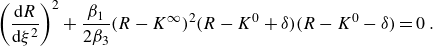 \begin{equation} \left (\frac {{\textrm d}R}{{\textrm d} \xi ^{2}}\right )^{2} +\frac {\beta _1}{2\beta _3}(R-K^\infty )^{2}(R-K^0+\delta )(R-K^0-\delta ) = 0\,. \end{equation}
Here $K^\infty$
represents the far-field value of the solution and
$K^\infty$
represents the far-field value of the solution and $K^0$
denotes the limiting value of the temporary wavenumber transition. The temporary downshifting solution corresponds to the case in which
$K^0$
denotes the limiting value of the temporary wavenumber transition. The temporary downshifting solution corresponds to the case in which $K^0\lt K^\infty$
, to which we restrict our discussion. Comparisons with (4.10) give that these take one of the following pairs of values:
$K^0\lt K^\infty$
, to which we restrict our discussion. Comparisons with (4.10) give that these take one of the following pairs of values:
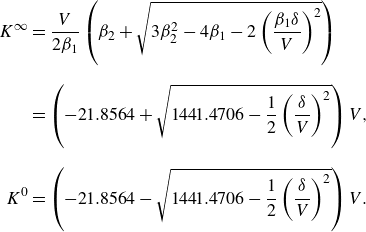 \begin{align} K^\infty &= \frac {V}{2\beta _1} \left (\beta _2 + \sqrt {3\beta _2^{2}-4\beta _1-2 \left (\frac {\beta _1\delta }{V}\right )^{2}}\right ) \nonumber\\[8pt] &= \left (-21.8564 + \sqrt {1441.4706 - \frac{1}{2}\left (\frac {\delta }{V}\right )^{2}}\right ) V, \nonumber\\[8pt] K^0 &= \left (-21.8564 - \sqrt {1441.4706 - \frac{1}{2}\left (\frac {\delta }{V}\right )^{2}}\right ) V. \end{align}
Thus, one may obtain the positive-polarity solitary wave solution (Kamchatnov et al. Reference Kamchatnov, Kuo, Lin, Horng, Gou, Clift, El and Grimshaw2012):
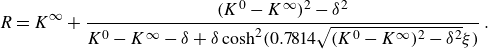 \begin{equation} R = K^\infty +\frac {(K^0-K^\infty )^{2}-\delta ^{2}}{K^0 -K^\infty -\delta +\delta \cosh ^{2}(0.7814\sqrt {(K^0-K^\infty )^{2}-\delta ^{2}}\xi )}\,. \end{equation}
As the parameter $\delta \lt 0$
approaches zero, the solitary wave becomes the previously mentioned tabletop solitary wave with amplitude close to
$\delta \lt 0$
approaches zero, the solitary wave becomes the previously mentioned tabletop solitary wave with amplitude close to $K^0-K^\infty$
. This profile can be tested in numerical simulations in order to deduce its stability and robustness in the water-wave problem via the use of reduced modelling. Such discussion can be found in section § 6.
$K^0-K^\infty$
. This profile can be tested in numerical simulations in order to deduce its stability and robustness in the water-wave problem via the use of reduced modelling. Such discussion can be found in section § 6.
6. Numerical validation of the phase dynamics solutions
In order to verify the theoretical conclusions, arrived at from the phase dynamics analysis, we resort to a numerical investigation of a system representative of the water-wave problem. We use the simplest water-wave model which contains the essential wave dynamics coupled to the mean flow, namely the Benney–Roskes system in (2.32)–(2.34). The Benney–Roskes system possesses the same characteristic features, elliptic–hyperbolic transition and phase dynamical picture as the full water-wave problem in the case where $\mu ,\,\tau$
in (2.5) are held fixed. Towards this end, we expect the tabletop solitary wave solution (5.6) to remain close to an exact solution within the Benney–Roskes system.
$\mu ,\,\tau$
in (2.5) are held fixed. Towards this end, we expect the tabletop solitary wave solution (5.6) to remain close to an exact solution within the Benney–Roskes system.
To initialise the simulations, we use the solution (5.6) in dimensional form and construct $A,B$
and
$A,B$
and $W$
according to (A3) (accounting for the fact that the smallness of
$W$
according to (A3) (accounting for the fact that the smallness of $a$
and
$a$
and $b$
has been factored out via
$b$
has been factored out via $\epsilon$
). In terms of the Benney–Roskes variables, the initial condition is constructed as
$\epsilon$
). In terms of the Benney–Roskes variables, the initial condition is constructed as
 \begin{align} A = \sqrt {|A_0|^{2}-0.9171 \tilde {\varepsilon } U}\,, \qquad B = B_0+0.8220\tilde {\varepsilon } U\,,\qquad W = W_0+ 3.4527 \tilde {\varepsilon } U\,, \end{align}
where $U$
is taken to be the tabletop solution. The small parameter
$U$
is taken to be the tabletop solution. The small parameter $\tilde {\varepsilon } = \varepsilon /\epsilon$
is a reduced small parameter which accounts for the small scale for which the Benney–Roskes system is operational,
$\tilde {\varepsilon } = \varepsilon /\epsilon$
is a reduced small parameter which accounts for the small scale for which the Benney–Roskes system is operational, $\epsilon$
. For simplicity we choose
$\epsilon$
. For simplicity we choose $|A_0|^{2} = 1$
and
$|A_0|^{2} = 1$
and $B_0 = W_0 = 0$
. This tabletop solution’s width (via choice of
$B_0 = W_0 = 0$
. This tabletop solution’s width (via choice of $\delta$
) is chosen so that the added perturbation contributes no additional mass to the Stokes wave to leading order on a principal domain of length
$\delta$
) is chosen so that the added perturbation contributes no additional mass to the Stokes wave to leading order on a principal domain of length $L$
(typically, 80 wavelengths to ensure the tabletop is sufficiently flat), so that
$L$
(typically, 80 wavelengths to ensure the tabletop is sufficiently flat), so that
 \begin{align} \int _{-L/2}^{L/2}U(\xi ,T) \, {\textrm d}\xi = 0. \end{align}
We then inflate our computational domain by some factor of order 10, depending on the simulation time and distance from the Benjamin–Feir threshold, to ensure recursion does not occur in our numerical solution as discussed in § 5.1. Later wavenumber properties are then computed on the principal domain of length $L$
. We choose the reference wavenumber
$L$
. We choose the reference wavenumber $k_0$
to be unity and control the distance to the Benjamin–Feir threshold via the choice of
$k_0$
to be unity and control the distance to the Benjamin–Feir threshold via the choice of $h_0\in [1.3, 1.3626]$
to ensure hyperbolicity of the underlying dynamics but to remain close to the modulation instability threshold. The smallness parameter of the Stokes waves is chosen as
$h_0\in [1.3, 1.3626]$
to ensure hyperbolicity of the underlying dynamics but to remain close to the modulation instability threshold. The smallness parameter of the Stokes waves is chosen as $\epsilon \sim 10^{-1}$
to align with typical experimental values for the steepness, and we note that this latter choice impacts simulation times due to its presence within the amplitude’s evolution. We set
$\epsilon \sim 10^{-1}$
to align with typical experimental values for the steepness, and we note that this latter choice impacts simulation times due to its presence within the amplitude’s evolution. We set $\varepsilon \sim \epsilon ^{2}$
so that
$\varepsilon \sim \epsilon ^{2}$
so that $\tilde {\varepsilon } \sim \epsilon$
in order to remain in the domain of asymptotic validity of the phase dynamics. For the time integration, we simulate in a periodic domain using an exponential time differencing scheme with Runge–Kutta timestepping of order 4 (Cox & Matthews Reference Cox and Matthews2002) with the stability modifications outlined within Kassam & Trefethen (Reference Kassam and Trefethen2005). This numerical scheme has been verified in a number of ways, including verification that the system conserves mass to
$\tilde {\varepsilon } \sim \epsilon$
in order to remain in the domain of asymptotic validity of the phase dynamics. For the time integration, we simulate in a periodic domain using an exponential time differencing scheme with Runge–Kutta timestepping of order 4 (Cox & Matthews Reference Cox and Matthews2002) with the stability modifications outlined within Kassam & Trefethen (Reference Kassam and Trefethen2005). This numerical scheme has been verified in a number of ways, including verification that the system conserves mass to $10^{-3}\,\%$
accuracy, that it admits the expected soliton solution when restricted to only the envelope equation (2.32) with
$10^{-3}\,\%$
accuracy, that it admits the expected soliton solution when restricted to only the envelope equation (2.32) with $W=B=0$
and that when restricted to the shallow-water components (2.33) and (2.34) with
$W=B=0$
and that when restricted to the shallow-water components (2.33) and (2.34) with $A=0$
the solution generates two profiles which move at the characteristic speeds
$A=0$
the solution generates two profiles which move at the characteristic speeds $ -c_g \pm \sqrt {g h_0}$
. Momentum is not conserved in the Benney–Roskes system, as we discuss later within this section in relation to downshifting.
$ -c_g \pm \sqrt {g h_0}$
. Momentum is not conserved in the Benney–Roskes system, as we discuss later within this section in relation to downshifting.


A representative example of the outcome of these simulations appears in figure 1. What is observed is that the initial tabletop lump splits into four components, two associated with the long-wave speed of the shallow-water component and two associated with the wave’s group velocity. The latter two components emerge much later than the former as one would expect, and the amplitudes of these modes differ owing to the higher-order terms present in the phase dynamical ansatz. All profiles maintain their general form within the simulation times, although one should note that the profiles associated with the group velocity can develop dispersive shocks at their leading edge if the initial data are large enough. Whilst this is likely indicative that the initial condition is outside the remit of the validity of the phase dynamics, this shock formation does not significantly impact the observations related to the wavenumber discussed below. In fact, this appears to be more reflective of the experimental observations of downshifting observed by Lake et al. (Reference Lake, Yuen, Rungaldier and Ferguson1977), where the transition occurred via a modulation–demodulation cycle.
We may also visualise the impact of these results on the original Stokes wave, which is done by reconstructing the free surface according to
 \begin{align} \eta = \epsilon A {\textrm e}^{1 k_0 X/\varepsilon }+\text{c.c.} +\varepsilon ^{2} B+\cdots , \end{align}
where we have focused on the leading-order wave–mean-flow effects in this reconstruction. These can be seen in figure 2, which highlights that the amplitude increase comes together with a drop in the mean fluid depth. Further, one can observe the presence of a slight change in wavenumber either side of the transition. This confirms the theoretical observations of this paper that a downshift in wavenumber comes with an amplitude increase and mean fluid level decrease (cf. (A3)).
We may also use these simulations to investigate the behaviour of the wavenumber of the Stokes wave. In the framework of the Benney–Roskes system, this relates to the full surface wave’s wavenumber $k$
via
$k$
via
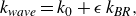 \begin{align} k_{\textit{wave}} = k_0+\epsilon \, k_{\textit{BR}}, \end{align}
where $k_{\textit{BR}}$
denotes the wavenumber extracted from the simulation. There are two key approaches we take to extract this perturbative wavenumber within the simulations. Our first approach is to extract the local wavenumber behaviour of the wave amplitude via the definition
$k_{\textit{BR}}$
denotes the wavenumber extracted from the simulation. There are two key approaches we take to extract this perturbative wavenumber within the simulations. Our first approach is to extract the local wavenumber behaviour of the wave amplitude via the definition
 \begin{equation} k_{\textit{BR}} = k_{local}(X,T) = \textrm {Im} \left [\partial _X\ln \left (\frac {A}{|A|}\right )\right ]\,, \end{equation}
where $\textrm {Im}$
indicates that the imaginary part is taken. An example of this extracted local wavenumber for a simulation appears in figure 3. We observe that there are three significant contributors to the local wavenumber change, two from the group velocity modes and one from the long-wave mode. This latter mode emerges first and corresponds to an increase in wavenumber, and although this is not associated with the wavenumber transitions we intend to study it is not unexpected as this will correspond to another seemingly linear phase dynamic (cf. § 3). Of the two modes associated with the group velocity, the larger-amplitude right-moving mode is responsible for the decrease in wavenumber and is significantly larger than the increase in local wavenumber of the other mode.
$\textrm {Im}$
indicates that the imaginary part is taken. An example of this extracted local wavenumber for a simulation appears in figure 3. We observe that there are three significant contributors to the local wavenumber change, two from the group velocity modes and one from the long-wave mode. This latter mode emerges first and corresponds to an increase in wavenumber, and although this is not associated with the wavenumber transitions we intend to study it is not unexpected as this will correspond to another seemingly linear phase dynamic (cf. § 3). Of the two modes associated with the group velocity, the larger-amplitude right-moving mode is responsible for the decrease in wavenumber and is significantly larger than the increase in local wavenumber of the other mode.
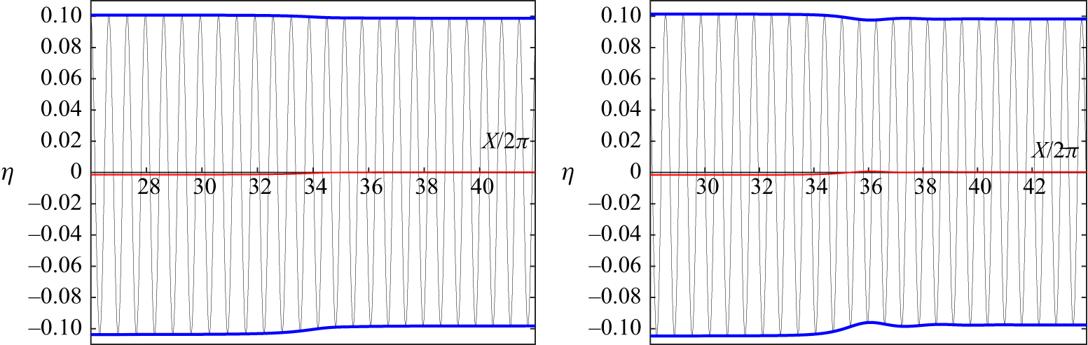
Figure 2. Visualisation of the free surface $\eta$
reconstructed from the numerical solution of the Benney–Roskes system at the final simulation time for the simulations of figure 1.
$\eta$
reconstructed from the numerical solution of the Benney–Roskes system at the final simulation time for the simulations of figure 1.


The second approach we take to determine wavenumber behaviour, particularly the emergent wavenumber behaviour for the entire wavetrain solution, is to study the spectral mean, following Carter et al. (Reference Carter, Henderson and Butterfield2019). It is defined by
 \begin{equation} k_{\textit{BR}} = k_m(T) = \frac {i\int AA^*_X-A^*A_X \, {\textrm d}X }{2\int |A|^{2} \, {\textrm d}X} \equiv \frac {\int k |\hat {A}|^{2} \, {\textrm d}k}{\int |\hat {A}|^{2} \, {\textrm d}k}, \end{equation}
where $\hat {A}(k,T)$
is the Fourier transform of the wave amplitude
$\hat {A}(k,T)$
is the Fourier transform of the wave amplitude $A$
. Whilst the momentum
$A$
. Whilst the momentum ${\mathscr{P}} = \int k|\hat {A}|^{2} \, {\textrm d}k$
is conserved in the dynamics of the nonlinear Schrödinger equation, it is not necessarily conserved under Benney–Roskes dynamics as
${\mathscr{P}} = \int k|\hat {A}|^{2} \, {\textrm d}k$
is conserved in the dynamics of the nonlinear Schrödinger equation, it is not necessarily conserved under Benney–Roskes dynamics as
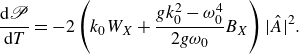 \begin{equation} \frac {{\textrm d} {\mathscr{P}}}{{\textrm d}T} = -2\left (k_0 W_X+\frac {gk_0^{2}-\omega _0^4}{2g\omega _0}B_X \right ) |\hat {A}|^{2} .\end{equation}
It is worth noting that the right-hand side of the above expression is not sign definite, and so upshifting of the spectral mean is also permitted. We also note that the (total) wave mass (i.e. the denominator of (6.6)) is conserved under both the nonlinear Schrödinger dynamics and the Benney–Roskes dynamics, but the mass on the domain that we examine, namely the original domain of length $L$
, the mass will decrease as the long-wave modes leave this portion of the domain. This causes the mass in this domain of interest to decrease but it does so almost negligibly. This lack of conservation of spectral mean permits the spectral mean to change over the wavetrain’s evolution, and we find that it decreases as depicted in figure 4. It depicts what is typical of a simulation with the prescribed set-up: the wavenumber drops significantly as the long-wave modes propagate out from the initial tabletop and subsequently out of the domain of interest, before slowly increasing (i.e. a minor upshift, as permitted by (6.7)) to a negative asymptotic value. This value is reasonably close to the arithmetic mean of the local wavenumbers of each tabletop solution, suggesting that the spectral mean is the result of these wavenumber shifts. It confirms, however, that the tabletop solution is the source of the negative spectral mean value and that it remains stable over the course of its propagation.
$L$
, the mass will decrease as the long-wave modes leave this portion of the domain. This causes the mass in this domain of interest to decrease but it does so almost negligibly. This lack of conservation of spectral mean permits the spectral mean to change over the wavetrain’s evolution, and we find that it decreases as depicted in figure 4. It depicts what is typical of a simulation with the prescribed set-up: the wavenumber drops significantly as the long-wave modes propagate out from the initial tabletop and subsequently out of the domain of interest, before slowly increasing (i.e. a minor upshift, as permitted by (6.7)) to a negative asymptotic value. This value is reasonably close to the arithmetic mean of the local wavenumbers of each tabletop solution, suggesting that the spectral mean is the result of these wavenumber shifts. It confirms, however, that the tabletop solution is the source of the negative spectral mean value and that it remains stable over the course of its propagation.
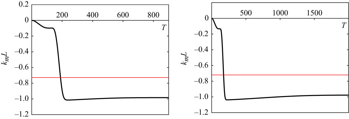
Figure 4. Spectral mean of the wavenumbers associated with the profiles in figure 1 as a function of time. The red line denotes the arithmetic mean of the long-time local wavenumber plateau values.
What the Benney–Roskes system also allows us to do is to explore the elliptic (i.e. modulationally unstable) regime, unlike the phase dynamical description. What we do find, despite the phase dynamical description being invalid here, is that the same trend of frequency downshifting persists and in its initial stages follows the hyperbolic regime with an example appearing in figure 5. As the modulation instability sets in, it works to improve the downshift substantially and decreases the wavenumber much further than the modulationally stable wavetrain close to threshold. We also observe that the transfer of energy in the power spectrum biases lower wavenumbers in line with the the observations from experiments (Lake et al. Reference Lake, Yuen, Rungaldier and Ferguson1977; Melville Reference Melville1982; Su et al. Reference Su, Bergin, Marler and Myrick1982). We re-emphasise that there are no dissipative effects here – this bias towards lower wavenumbers in the numerical simulation is entirely mean-flow-driven. It does, however, remain an open question whether the wave profiles within these simulations become steep enough to break and thus for dissipation to play a role in this regime, but these simulations show that this is not required for the downshifting phenomena in the modulationally unstable regime. What we do not see in this case is recurrence or restabilisation, instead seeing the formation of a soliton train which initially forms at the edges of the splitting tabletop solitary wave and expands over the simulation time.
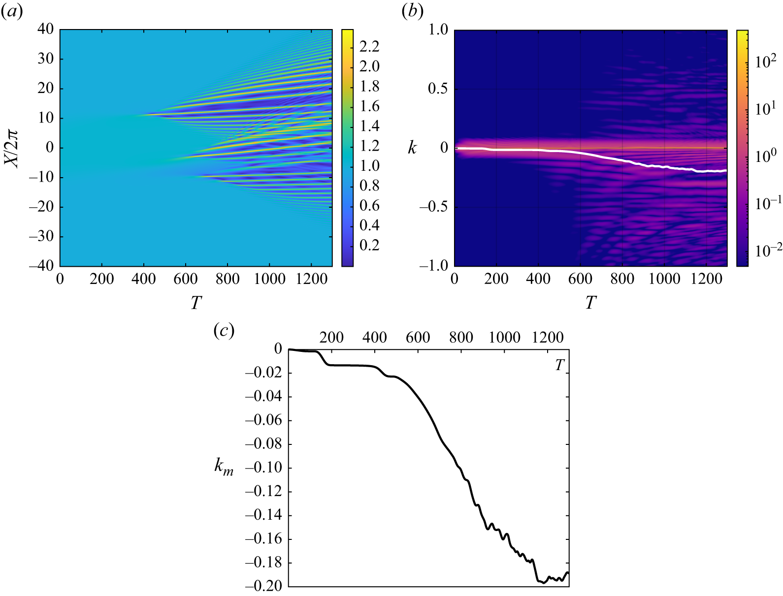
Figure 5. A numerical simulation for $k_0h_0 = 1.4$
, showing the amplitude (a), power spectral density (b) and spectral mean wavenumber (c). The spectral mean wavenumber is marked with a white line on the power spectral density in (b).
$k_0h_0 = 1.4$
, showing the amplitude (a), power spectral density (b) and spectral mean wavenumber (c). The spectral mean wavenumber is marked with a white line on the power spectral density in (b).
7. Concluding remarks
This paper has introduced a mechanism for water waves to undergo a permanent frequency downshift without dissipative effects. Mathematically, it is due to a local loss of genuine nonlinearity arising at the Benjamin–Feir transition that introduces higher-order effects that support front profiles for the wavenumber’s evolution. Energetically, it occurs because of a decrease in energy which restabilises the Stokes wave. This energetic perspective helps to reinforce the observations that the energy exchange to the lower sideband is much higher than that to upper sidebands. This paper highlights that these effects are due to mean-flow effects present in the problem. As a consequence, one of the key conclusions of this paper is that the interplay between wave motion and mean flow is important and should be more carefully considered in the water-wave problem. Our study here suggests that slaving the mean-flow effects to the wave motion, either as part of a reduction to nonlinear Schrödinger (Ablowitz & Segur Reference Ablowitz and Segur1981; Johnson Reference Johnson1997) or the earlier treatments of the water-wave problem from a modulation perspective (Whitham Reference Whitham1967, Reference Whitham2011), omits important aspects of the dynamics of Stokes waves.
This paper has demonstrated numerically that downshifting is the wave’s preferred outcome in the neighbourhood (and in the case of the elliptic regime, the presence of) modulation instability. It has shown this preference for downshifting via a reduction of the full water-wave problem that accounts for both wave and mean-flow evolution in space and time, the Benney–Roskes system, revealing behaviour absent from amplitude-only models and again emphasising that these outcomes must be attributed to the wave–mean-flow interplay of the problem. The numerical results also underscore that it is possible to have this downshift be permanent and not part of a recurrence cycle, as previously argued to be the only possibility in conservative systems (Lo & Mei Reference Lo and Mei1985). Whilst this is a simulation of an approximation of the full water-wave problem, it provides an important first step in the verification of this phenomenon in the full water-wave problem. The requirement of spatiotemporal evolution to observe the downshifting phenomenon suggests that solvers that seek minimiser (such as the scheme of Ablowitz, Fokas & Musslimani (Reference Ablowitz, Fokas and Musslimani2006)) may not be the appropriate way to validate this phenomenon, and instead one should utilise either conformal (Dyachenko, Zakharov & Kuznetsov Reference Dyachenko, Zakharov and Kuznetsov1996; Choi & Camassa Reference Choi and Camassa1999) or canonical (Craig & Sulem Reference Craig and Sulem1993) formulations to explore the phenomenon within the full Euler equations.
We re-emphasise that, whilst the explanation for downshifting without reliance on dissipation is an important step forward in our understanding of the phenomenon, dissipation remains one possible (and provably successful) mechanism for decreases in spectral peaks (Carter et al. Reference Carter, Henderson and Butterfield2019). Particularly, the dissipative description is valid deep into the elliptic regime, well outside of the transition regime to which the phase dynamical description of this paper is applicable. An important future avenue for study will be to compare the interplay of these effects and in which regimes one effect may dominate over the other and to the degree to which it does so.
It is worth noting that this study of mean-flow-driven downshifting highlights that upshifting of the Stokes wave is also a possibility, highlighted by the form of the heteroclinic connection as well as the connection to the Benney–Roskes equation. Particularly, (6.7) demonstrates that the spectral mean may increase in some instances, as has been reported experimentally (Ma et al. Reference Ma, Dong, Perlin, Ma and Wang2012). The energetic arguments of § 5, which suggest long-term downshifting, only hold in the hyperbolic case and cease to be valid in the elliptic regime. This suggests upshifting is only possible once the Benjamin–Feir instability is operational, but this should be verified as part of further studies into this phenomenon.
The assumption of gravity waves is important here, as it ensures that $\omega^{\prime\prime}_0 \neq 0$
for any choice of
$\omega^{\prime\prime}_0 \neq 0$
for any choice of $k$
and thus ensures the non-degeneracy of the phase dynamics. The inclusion of capillary effects introduces a new modulation stability boundary at points where
$k$
and thus ensures the non-degeneracy of the phase dynamics. The inclusion of capillary effects introduces a new modulation stability boundary at points where $\omega^{\prime\prime}_0 = 0$
, and such points cause every coefficient in (3.9) to become zero. To rebalance the phase dynamics in this case, one must include higher-order dispersive effects in addition to the considerations made for the scenario of this paper. The result is a fully extended version of the two-way Boussinesq equation which supports localised solutions as well as fronts.
$\omega^{\prime\prime}_0 = 0$
, and such points cause every coefficient in (3.9) to become zero. To rebalance the phase dynamics in this case, one must include higher-order dispersive effects in addition to the considerations made for the scenario of this paper. The result is a fully extended version of the two-way Boussinesq equation which supports localised solutions as well as fronts.
The mechanism proposed here is universal in that it does not rely on a particular governing equation, just on the fact that the equations are generated by a Lagrangian and there exists a multi-parameter family of periodic or multi-periodic travelling waves, with parameter values at which two characteristics coalesce, and furthermore the nonlinearity in the re-modulation is cubic. Indeed, generalisations of the water-wave problem (inclusion of surface tension, variable density, electromagnetic fields, etc.), at both finite amplitude and weakly nonlinear limit, would be settings where the above scenario is likely to occur.
Although downshifting has been shown to be the only energetically viable result in the gravity water-wave problem at the threshold of modulation instability, upshifts are also theoretically possible in other physical systems. For example, Whistler waves in the magnetosphere may undergo a downshift or an upshift depending on whether they are travelling parallel or orthogonal to the background magnetic field (Omura, Katoh & Summers Reference Omura, Katoh and Summers2008; Omura Reference Omura2021; Ratliff & Allanson Reference Ratliff and Allanson2023). The analysis performed here is likely to explain when this is permissible and will be due to how the amplitude varies with the mean-flow element (which for plasmas takes the role of velocity and number density perturbations), in comparison with the principal change in the wavenumber and frequency.
Acknowledgements
D.J.R. would like to thank the participants of the Dispersive Hydrodynamics programme, especially P. Sprenger and P. Milewski, for their invaluable discussions throughout the development of this work.
Funding
The authors would like to thank the Isaac Newton Institute for Mathematical Sciences for support and hospitality during the programme Dispersive Hydrodynamics when work on this paper was undertaken. This work was supported by EPSRC grant number EP/R014604/1.
Declaration of interest
The authors report no conflict of interest.
Appendix A. Effect of mean velocity on the amplitudes $\boldsymbol\rm{a}$
and
$\boldsymbol\rm{b}$
$\boldsymbol\rm{a}$
and
$\boldsymbol\rm{b}$


The perturbative impact on the amplitude and mean flow of the Stokes wave, in the neighbourhood of fixed values $(a_0,b_0)$
, is given in this appendix. Using the definitions (2.12), (2.25) and (B2), we can show that the leading-order contributions to their change is
$(a_0,b_0)$
, is given in this appendix. Using the definitions (2.12), (2.25) and (B2), we can show that the leading-order contributions to their change is
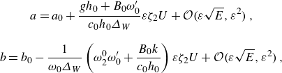 \begin{equation} \begin{gathered} a = a_0+\frac {gh_0+B_0\omega^{\prime}_0}{c_0h_0\varDelta_W}\varepsilon \zeta _2U+{\mathcal{O}}\big(\varepsilon \sqrt {E},\varepsilon ^{2}\big)\,, \\[8pt] b = b_0-\frac {1}{\omega _0\varDelta_W}\left (\omega _2^0\omega^{\prime}_0+\frac {B_0k}{c_0h_0}\right )\varepsilon \zeta _2 U+{\mathcal{O}}\big(\varepsilon \sqrt {E},\varepsilon ^{2}\big)\,, \end{gathered} \end{equation}
where $\zeta _2$
is the second component of the eigenvector
$\zeta _2$
is the second component of the eigenvector ${\boldsymbol{\zeta }}$
in (2.21). This expansion highlights that the primary effect on the Stokes waves arises from the mean-flow element of the problem, evident from the appearance of
${\boldsymbol{\zeta }}$
in (2.21). This expansion highlights that the primary effect on the Stokes waves arises from the mean-flow element of the problem, evident from the appearance of $\zeta _2$
, as opposed to being driven by the wave itself. The expressions preceding the perturbation
$\zeta _2$
, as opposed to being driven by the wave itself. The expressions preceding the perturbation $U$
represent recurring factors within the analysis, and so it is convenient to define the two quantities
$U$
represent recurring factors within the analysis, and so it is convenient to define the two quantities
 \begin{equation} {\mathscr{M}}_{1} = \frac {gh_0+B_0\omega^{\prime}_0}{c_0h_0\varDelta_W}\lt 0\,, \qquad {\mathscr{M}}_{2} = -\frac {1}{\omega _0\varDelta_W}\left (\omega _2^0\omega^{\prime}_0+\frac {B_0k}{c_0h_0}\right )\gt 0\,. \end{equation}
These quantities arise due to the variations of the wave amplitude and bulk flow due to the mean-flow effects and are important in characterising the impact of these effects on the dynamics of the wave. Evaluating these perturbations to the wave amplitude and bulk flow at the Benjamin–Feir transition, one finds
 \begin{equation} a = a_0-0.9171 \varepsilon U+{\mathcal{O}}\big(\varepsilon \sqrt {E},\varepsilon ^{2}\big), \qquad b = b_0+0.8220 \varepsilon U+{\mathcal{O}}\big(\varepsilon \sqrt {E},\varepsilon ^{2}\big). \end{equation}
As $\zeta _1\gt 0$
at the transition, one can infer that increases in the wavenumber, corresponding to positive
$\zeta _1\gt 0$
at the transition, one can infer that increases in the wavenumber, corresponding to positive $U$
, result in a decrease of amplitude and a rise (drop) in mean level, and vice versa. This is in line with the experimental observations of Lake et al. (Reference Lake, Yuen, Rungaldier and Ferguson1977). We may also use this information to infer the stability of the Stokes wave by assessing how the non-dimensional depth
$U$
, result in a decrease of amplitude and a rise (drop) in mean level, and vice versa. This is in line with the experimental observations of Lake et al. (Reference Lake, Yuen, Rungaldier and Ferguson1977). We may also use this information to infer the stability of the Stokes wave by assessing how the non-dimensional depth $kh$
changes near this transition. To leading order, this is
$kh$
changes near this transition. To leading order, this is
 \begin{align} kh = kh_0+2.0829\varepsilon U+{\mathcal{O}}\big(\varepsilon \sqrt {E},b,\varepsilon ^{2}\big)\,. \end{align}
As expected, the states which increase the wavenumber also increase $kh$
, but do so at a faster rate than the changes in the mean level that would otherwise balance it out.
$kh$
, but do so at a faster rate than the changes in the mean level that would otherwise balance it out.
Appendix B. Explicit expressions for matrix pencil entries
Explicit expressions for the entries of the matrix pencil $\textbf{E}(c)$
defined in (2.21) are given here:
$\textbf{E}(c)$
defined in (2.21) are given here:
 \begin{align} E_{11} & = \frac {g(c-c_g)^{2}}{\omega _0^{2}\varDelta_{W}} +\left [\frac {\omega^{\prime\prime}_0}{\omega _0}+\frac {c-c_g}{\omega _0}\left (\frac {(c-c_g-2\omega^{\prime}_0)}{\omega _0}+\frac {2}{c_0h_0\varDelta_W} (B_0\mu^{\prime}-g\tau^{\prime} )\right )\right ]E \nonumber\\[8pt] & \quad -\, \frac {2g(c-c_g)}{\omega _0\varDelta_W}\mu ^{\prime}kb, \nonumber\\[8pt] E_{12} &= -\frac {(c-c_g)(g h_0+B_0 (c-u))}{c_0^{2}kh_0\varDelta_{W}} \nonumber\\[8pt] & \quad +\left [\!\frac {c-c_g-\omega^{\prime}_0+c_0}{c_0^{2} k}+\frac {(gh_0+B_0(c-u) )}{c_0h_0\varDelta_W}\tau ^{\prime}-\frac {1}{\varDelta_W}\left (\frac { kB_0}{c_0h_0}+\omega _2^0 (c-u) \right )\mu ^{\prime} \!\right ]E \nonumber\\[8pt] & \quad +\, \frac {(gh_0+B_0(c-u) )}{c_0h_0\varDelta_W}\mu ^{\prime} b, \nonumber\\[8pt] E_{22} & = \frac {gh_0+2B_0(c-u)+B_0^{2}}{c_0^{2}h_0\varDelta_{W}}-\frac {\omega _2(gh_0-(c-u)^{2})}{\omega _0\varDelta_{W}}+b-\frac {E}{c_{0}^{2}}. \end{align}
This matrix has a right eigenvector associated with the characteristic (2.25) defined by $\textbf{E}(c){\boldsymbol{\zeta }}=0$
. It can be expanded for small amplitude to give
$\textbf{E}(c){\boldsymbol{\zeta }}=0$
. It can be expanded for small amplitude to give
 \begin{align} &{\boldsymbol{\zeta }} = \begin{pmatrix} \zeta _1\\[3pt] \zeta _2 \end{pmatrix} = \pm \sqrt {\omega^{\prime\prime}_0 \omega _2^{\textit{eff}}} \boldsymbol{\chi }\nonumber\\[8pt] & +\, \sqrt {E}\!\left [ \! C_2\boldsymbol{\chi }- \!\begin{pmatrix} \dfrac {B_0 \omega^{\prime\prime}_0 \omega _2^{\textit{eff}}}{c_0h_0\varDelta_W}+\dfrac {\omega^{\prime}_0}{c_0}-1+\dfrac {1}{\varDelta_W}\left (\omega _2^0\omega^{\prime}_0+\dfrac {kB_0}{c_0h_0}\right )\mu ^{\prime}-\dfrac {k(B_0\omega^{\prime}_0 + gh_0)}{h_0\varDelta_W}\tau ^{\prime}\\[14pt] \omega^{\prime\prime}_0 \left (1+\frac {g \omega _2^{\textit{eff}}}{\omega _0\varDelta_W} \!\right ) \end{pmatrix} \!\right ]\nonumber\\[8pt] & \pm\, E \left [C_3 \boldsymbol{\chi } +\sqrt {\omega^{\prime\prime}_0 \omega _2}\left ( \begin{pmatrix} \frac {1}{c_0}\\[5pt] 0 \end{pmatrix}+\frac {2C_2}{\varDelta_W} \begin{pmatrix} \mu \\[5pt] -\frac {g}{\omega _0} \end{pmatrix} \right )\right ] + \mathcal{O}\big(E^{3/2}\big),\end{align}
with
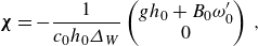 \begin{align} {\boldsymbol{\chi }} = -\frac {1}{c_0h_0\varDelta_W} \begin{pmatrix} gh_0+B_0\omega^{\prime}_0\\ 0 \end{pmatrix}\,, \end{align}
where $C_3$
is a further term in the amplitude expansion of the characteristic. It is not given here as it does not contribute to the analysis at the orders considered.
$C_3$
is a further term in the amplitude expansion of the characteristic. It is not given here as it does not contribute to the analysis at the orders considered.


 Open access