


1. Introduction
Ventilated partial- and super-cavitation (VPC and VSC, respectively) are characterised by gas cavities formed by injecting non-condensable gas behind a ‘cavitator’ (Logvinovich Reference Logvinovich1969). This technique has gained significant attention due to its potential application for drag reduction on ship hulls by forming an air cavity and reducing the near-wall density (Ceccio Reference Ceccio2010). Ventilated supercavities have also found applications in hydraulic engineering (Chanson Reference Chanson2010) and process industries (Rigby, Evans & Jameson Reference Rigby, Evans and Jameson1997) to mitigate deleterious effects of natural cavitation, such as wear, erosion and failure, all resulting from violent cloud implosion (Brennen Reference Brennen1995). The stability of ventilated cavities is crucial, as unstable ventilated cavities can get detached abruptly, leading to a sudden increase in drag forces. Insufficient ventilation may lead to cavity collapse, while excessive ventilation could result in cavity oscillation, both undesired and often detrimental (Ceccio Reference Ceccio2010). Hence, it is necessary to understand the exact flow conditions that govern the stability of ventilated cavities. Ventilated cavities are governed by incoming flow pressure ( $P_{0}$
) and velocity (
$P_{0}$
) and velocity ( $U_{0}$
), input gas injection rate (
$U_{0}$
), input gas injection rate ( $\dot Q_{in}$
), cavity pressure (
$\dot Q_{in}$
), cavity pressure ( $P_{c}$
) and cavitator geometry (area
$P_{c}$
) and cavitator geometry (area $A=WH$
, length scale
$A=WH$
, length scale $H$
). See figure 1 for the definitions of parameters. These parameters can be expressed as non-dimensional cavitation number (
$H$
). See figure 1 for the definitions of parameters. These parameters can be expressed as non-dimensional cavitation number ( $\sigma _{c}$
), Froude number (
$\sigma _{c}$
), Froude number ( $\textit{Fr}$
) and ventilation coefficient (
$\textit{Fr}$
) and ventilation coefficient ( $C_{qs}$
), defined as follows:
$C_{qs}$
), defined as follows:
 \begin{align} \sigma _{c} = \frac {P_{0}-P_{c}}{\frac {1}{2} \rho U_{0}^{2}}, \hspace {7mm} Fr = \frac {U_{0}}{\sqrt {gH}}, \hspace {7mm} C_{qs} = \frac {\dot Q_{in}}{U_{0}A}. \end{align}
Here $\rho$
and g are mass density and acceleration due to gravity, respectively. Ventilated cavities behind bluff bodies are formed when a part of the injected gas (
$\rho$
and g are mass density and acceleration due to gravity, respectively. Ventilated cavities behind bluff bodies are formed when a part of the injected gas ( $\dot Q_{in}$
) gets entrained in the separated flow (behind the cavitator), while the remainder of the gas is ejected (
$\dot Q_{in}$
) gets entrained in the separated flow (behind the cavitator), while the remainder of the gas is ejected ( $\dot Q_{out}$
) from the cavity closure region. The entrained gas, i.e. the gas that is dragged into the cavity, results in the growth of the cavity. Here, closure refers to the way a cavity closes itself and dictates the amount of gas ejected out of the cavity. The cavity closure also influences the cavity geometry (length, thickness and gas distribution), and, most importantly, the stability of the cavity. Hence, a thorough understanding of the cavity closure is imperative.
$\dot Q_{out}$
) from the cavity closure region. The entrained gas, i.e. the gas that is dragged into the cavity, results in the growth of the cavity. Here, closure refers to the way a cavity closes itself and dictates the amount of gas ejected out of the cavity. The cavity closure also influences the cavity geometry (length, thickness and gas distribution), and, most importantly, the stability of the cavity. Hence, a thorough understanding of the cavity closure is imperative.
Ventilated cavities, especially in three-dimensional axisymmetric cavitators, have been investigated extensively in the past. It was shown that at a high $\textit{Fr}$
, the cavity closure is characterised by a re-entrant jet (Epshteyn Reference Epshteyn1961; Logvinovich Reference Logvinovich1969; Karn, Arndt & Hong Reference Karn, Arndt and Hong2016). However, at low
$\textit{Fr}$
, the cavity closure is characterised by a re-entrant jet (Epshteyn Reference Epshteyn1961; Logvinovich Reference Logvinovich1969; Karn, Arndt & Hong Reference Karn, Arndt and Hong2016). However, at low $\textit{Fr}$
, buoyancy effects result in lift generation and the formation of two vortex tubes at the closure (Semenenko Reference Semenenko2001). Karn et al. (Reference Karn, Arndt and Hong2016) explained these observations based on the pressure difference across the cavity closure (
$\textit{Fr}$
, buoyancy effects result in lift generation and the formation of two vortex tubes at the closure (Semenenko Reference Semenenko2001). Karn et al. (Reference Karn, Arndt and Hong2016) explained these observations based on the pressure difference across the cavity closure ( $\Delta \tilde {P}$
): a higher
$\Delta \tilde {P}$
): a higher $\Delta \tilde {P}$
gave rise to a re-entrant jet similar to natural partial cavities (Knapp Reference Knapp1958; Callenaere et al. Reference Callenaere, Franc, Michel and Riondet2001), while a lower
$\Delta \tilde {P}$
gave rise to a re-entrant jet similar to natural partial cavities (Knapp Reference Knapp1958; Callenaere et al. Reference Callenaere, Franc, Michel and Riondet2001), while a lower $\Delta \tilde {P}$
resulted in vortex tube closure. At significantly high ventilation inputs, oscillating cavities called pulsating cavities (PCs) were identified (Silberman & Song Reference Silberman and Song1961; Skidmore Reference Skidmore2016). For the three-dimensional fence-type cavitator (Barbaca, Pearce & Brandner Reference Barbaca, Pearce and Brandner2017), similar observations were made: cavities with re-entrant flow were seen at higher
$\Delta \tilde {P}$
resulted in vortex tube closure. At significantly high ventilation inputs, oscillating cavities called pulsating cavities (PCs) were identified (Silberman & Song Reference Silberman and Song1961; Skidmore Reference Skidmore2016). For the three-dimensional fence-type cavitator (Barbaca, Pearce & Brandner Reference Barbaca, Pearce and Brandner2017), similar observations were made: cavities with re-entrant flow were seen at higher $\textit{Fr}$
, while at lower
$\textit{Fr}$
, while at lower $\textit{Fr}$
the cavity was seen to split into two separate branches with re-entrant flow on each branch. All the cavities in this study had a re-entrant flow closure, possibly due to the high Froude number (
$\textit{Fr}$
the cavity was seen to split into two separate branches with re-entrant flow on each branch. All the cavities in this study had a re-entrant flow closure, possibly due to the high Froude number ( $\textit{Fr}$
) employed in that study. Ventilated cavities behind a two-dimensional cavitator have received relatively less attention in the literature despite their wide application for partial cavity drag reduction on ships (Mäkiharju et al. Reference Mäkiharju, Elbing, Wiggins, Schinasi, Vanden-Broeck, Perlin, Dowling and Ceccio2013a
; Barbaca, Pearce & Brandner Reference Barbaca, Pearce and Brandner2018). In a wall-bounded two-dimensional cavitator, Qin et al. (Reference Qin, Wu, Wu and Hong2019) observed a twin-branch cavity, analogous to vortex tube closure. Qin et al. (Reference Qin, Wu, Wu and Hong2019) also reported supercavities with dispersed bubbles at the closure, and cavities with re-entrant jet closure were not observed, likely due to the low Froude number (
$\textit{Fr}$
) employed in that study. Ventilated cavities behind a two-dimensional cavitator have received relatively less attention in the literature despite their wide application for partial cavity drag reduction on ships (Mäkiharju et al. Reference Mäkiharju, Elbing, Wiggins, Schinasi, Vanden-Broeck, Perlin, Dowling and Ceccio2013a
; Barbaca, Pearce & Brandner Reference Barbaca, Pearce and Brandner2018). In a wall-bounded two-dimensional cavitator, Qin et al. (Reference Qin, Wu, Wu and Hong2019) observed a twin-branch cavity, analogous to vortex tube closure. Qin et al. (Reference Qin, Wu, Wu and Hong2019) also reported supercavities with dispersed bubbles at the closure, and cavities with re-entrant jet closure were not observed, likely due to the low Froude number ( $\textit{Fr}\lt 6$
) considered in their study. In summary, distinct closure types are observed for different cavitator geometries.
$\textit{Fr}\lt 6$
) considered in their study. In summary, distinct closure types are observed for different cavitator geometries.
Ventilated cavities in the wake of two-dimensional bluff bodies remain sparsely explored. Ventilated and natural cavitation behind bluff bodies are influenced by the near- and far-wake flow. Single-phase wake flows behind bluff bodies have been studied by several researchers (Roshko Reference Roshko1955; Gerrard Reference Gerrard1966; Balachandar, Mittal & Najjar Reference Balachandar, Mittal and Najjar1997). One of the main features of non-cavitating/single-phase wake flows is wake formation length which depends on the object size and confinement, if present. To this end, natural cavitation in wake flows has also been studied by Young & Holl (Reference Young and Holl1966), Ramamurthy & Bhaskaran (Reference Ramamurthy and Bhaskaran1978), Belahadji, Franc & Michel (Reference Belahadji, Franc and Michel1995) and more recently by Brandao, Bhatt & Mahesh (Reference Brandao, Bhatt and Mahesh2019), Wu et al. (Reference Wu, Deijlen, Bhatt, Ganesh and Ceccio2021). Some of the main findings of all these studies are the dependence of natural cavities on the wake properties such as formation length, vorticity accumulation, and compressibility of the liquid–vapour mixture. Ventilated supercavities in the wake of two-dimensional bluff bodies were studied by Butuzov (Reference Butuzov1967), Laali & Michel (Reference Laali and Michel1984), Michel (Reference Michel1984) with an emphasis on cavity pulsation. For instance, Michel (Reference Michel1984) reported long PCs with wavelengths of the order of the wedge base height.
The cavity closure influences the gas entrainment/ejection rate into/out of the cavity. Understanding the gas entrainment and ejection mechanisms is important to establish and maintain ventilated cavities efficiently. Spurk & Konig (Reference Spurk and Konig2002) postulated that the injected gas is carried to the closure by a growing internal boundary layer at the gas–liquid interface, where it is ejected out in the form of toroidal vortices. For wall-bounded cavitators, Qin et al. (Reference Qin, Wu, Wu and Hong2019) proposed that the recirculation region interface is responsible for entraining the gas bubbles into the separated shear layer, which are then carried away downstream. This was verified experimentally by Wu et al. (Reference Wu, Liu, Shao and Hong2019a ) in a study on the gas flow inside the ventilated cavity using particle image velocimetry (PIV). Although the gas entrainment mechanisms were found to be identical for different cavity closures, the gas leakage mechanisms were seen to be different. Various gas ejection mechanisms are identified in ventilated cavities: (i) gas ejection due to a re-entrant jet (Spurk & Konig Reference Spurk and Konig2002; Kinzel & Maughmer Reference Kinzel, Maughmer and Duque2010; Barbaca et al. Reference Barbaca, Pearce and Brandner2017), (ii) vortex tube gas leakage (Cox & Clayden Reference Cox and Clayden1955; Semenenko Reference Semenenko2001), (iii) pulsation of cavities (Michel Reference Michel1984; Karn et al. Reference Karn, Arndt and Hong2016; Skidmore Reference Skidmore2016) and (iv) surface waves pinching the cavity (Zverkhovskyi Reference Zverkhovskyi2014). Furthermore, Qin et al. (Reference Qin, Wu, Wu and Hong2019) observed the role of capillary wave pinch-off in gas ejection in twin-branched cavities.
Despite qualitative observations, studies dedicated to the quantification of gas ejection rates out of cavities ( $\dot {Q}_{out}$
) for different cavity closures are scarce. Quantifying gas ejection rates is essential in formulating empirical models, validating numerical models, and furthering our understanding of the underlying flow physics at cavity closures. This also enables better prediction of gas ventilation demands under different flow conditions (
$\dot {Q}_{out}$
) for different cavity closures are scarce. Quantifying gas ejection rates is essential in formulating empirical models, validating numerical models, and furthering our understanding of the underlying flow physics at cavity closures. This also enables better prediction of gas ventilation demands under different flow conditions ( $\textit{Fr}$
and
$\textit{Fr}$
and $C_{qs}$
). Recently, Shao et al. (Reference Shao, Li, Yoon and Hong2022) used digital inline holography (DIH) to quantify the instantaneous
$C_{qs}$
). Recently, Shao et al. (Reference Shao, Li, Yoon and Hong2022) used digital inline holography (DIH) to quantify the instantaneous $\dot {Q}_{out}$
for stable cavity closure types. While stable cavity types have received adequate attention in the literature, transitional cavity closure types during the formation of a supercavity remain unexplored despite their wide engineering implications. The ventilation demands to establish and maintain VCs can be estimated more accurately by studying the gas ejection of these transitional VCs. Furthermore, hysteresis in VC formation plays a significant role in determining the accurate ventilation demands, i.e. for a given ventilation (
$\dot {Q}_{out}$
for stable cavity closure types. While stable cavity types have received adequate attention in the literature, transitional cavity closure types during the formation of a supercavity remain unexplored despite their wide engineering implications. The ventilation demands to establish and maintain VCs can be estimated more accurately by studying the gas ejection of these transitional VCs. Furthermore, hysteresis in VC formation plays a significant role in determining the accurate ventilation demands, i.e. for a given ventilation ( $C_{qs}$
), a ventilated cavity can assume a different length and closure depending upon how the ventilation condition was reached (Kawakami & Arndt Reference Kawakami and Arndt2011; Mäkiharju et al. 2013a; Karn et al. Reference Karn, Arndt and Hong2016). Ventilation hysteresis is widely reported in ventilated cavities, but the exact physical mechanism responsible for it remains unclear. The characterisation and implication of ventilation hysteresis are essential to devise control strategies for efficient drag-reduction and aeration systems.
$C_{qs}$
), a ventilated cavity can assume a different length and closure depending upon how the ventilation condition was reached (Kawakami & Arndt Reference Kawakami and Arndt2011; Mäkiharju et al. 2013a; Karn et al. Reference Karn, Arndt and Hong2016). Ventilation hysteresis is widely reported in ventilated cavities, but the exact physical mechanism responsible for it remains unclear. The characterisation and implication of ventilation hysteresis are essential to devise control strategies for efficient drag-reduction and aeration systems.
The lack of quantitative insights in ventilated cavities can be attributed to the challenges brought about by turbulence, frothiness and optical opaqueness of the flow. Wosnik & Arndt (Reference Wosnik and Arndt2013) attempted to estimate the void fraction and velocity fields in the frothy mixture of the VCs with laser-illuminated bubble images; however, the uncertainty in the measurements was high. Furthermore, PIV has been successful in only the clear part of supercavities, providing limited insights into the gas ejection mechanisms (Wang et al. Reference Wang, Huang, Zhang, Wang and Zhao2018; Wu et al. Reference Wu, Liu, Shao and Hong2019b ; Yoon et al. Reference Yoon, Qin, Shao and Hong2020). Holography is limited to the far-field, where individual ejected gas bubbles can be imaged (Shao et al. Reference Shao, Li, Yoon and Hong2022). Thus, conventional optical-based measurement techniques are untenable, especially at the liquid–gas–liquid interface and cavity closure region. High-fidelity numerical simulations such as direct numerical simulation are limited to low Reynolds numbers (Liu, Xiao & Shen Reference Liu, Xiao and Shen2023) due to the large density ratios and turbulent motions, with a wide range of scales in the flow (Madabhushi & Mahesh Reference Madabhushi and Mahesh2023). These shortcomings can be overcome by whole-field radiation-based measurement techniques such as time-resolved X-ray densitometry (Aliseda & Heindel Reference Aliseda and Heindel2021; Mäkiharju et al. Reference Mäkiharju, Gabillet, Paik, Chang, Perlin and Ceccio2013b ), wherein gas–liquid interfaces and the cavity closure region can be resolved reliably. Such time-resolved void fraction measurements can provide quantitative information in gas entrainment and leakage dynamics apart from time-averaged gas distribution in ventilated cavities. The void fraction fields are also indispensable for quantifying the compressibility effects in ventilated cavity flows, deemed crucial in natural cavitation flows (Ganesh, Makiharju & Ceccio Reference Ganesh, Mäkiharju and Ceccio2016; Gawandalkar & Poelma Reference Gawandalkar and Poelma2024). Further, void fraction profiles in ventilated cavities can be useful for validating numerical models aimed at accurately simulating complex ventilated cavity flows.
In this paper, we study the effect of gas entrainment in the wake of a two-dimensional wedge by systematically varying the flow inertia ( $\textit{Fr}$
) and gas injection rate (
$\textit{Fr}$
) and gas injection rate ( $C_{qs}$
). We identify four different types of ventilated cavities based on the closure topology, and determine the associated flow conditions on a regime map. The effect of
$C_{qs}$
). We identify four different types of ventilated cavities based on the closure topology, and determine the associated flow conditions on a regime map. The effect of $\textit{Fr}$
and
$\textit{Fr}$
and $C_{qs}$
on the cavity closure type, cavity geometry and gas ejection mechanism is studied in detail using two-dimensional time-resolved X-ray densitometry and high-speed imaging. The transitional cavity closures and the resulting gas ejection rates out of the cavity are quantified during the formation process using a simple gas balance based on a control volume approach. The ventilation hysteresis in the formation of supercavities is investigated systematically using two different ventilation strategies. We observe a substantial difference between the gas flux required to form and maintain a supercavity. Finally, a relationship between cavity closure and the resulting gas ejection rates influenced by the wake–gas interaction is proposed. The rest of the paper is organised into five additional sections. The experimental methodology is described in
$C_{qs}$
on the cavity closure type, cavity geometry and gas ejection mechanism is studied in detail using two-dimensional time-resolved X-ray densitometry and high-speed imaging. The transitional cavity closures and the resulting gas ejection rates out of the cavity are quantified during the formation process using a simple gas balance based on a control volume approach. The ventilation hysteresis in the formation of supercavities is investigated systematically using two different ventilation strategies. We observe a substantial difference between the gas flux required to form and maintain a supercavity. Finally, a relationship between cavity closure and the resulting gas ejection rates influenced by the wake–gas interaction is proposed. The rest of the paper is organised into five additional sections. The experimental methodology is described in $\S$
2. The fixed-length and transitional ventilated cavities are treated separately; the characteristics of ventilated cavities are described in detail in
$\S$
2. The fixed-length and transitional ventilated cavities are treated separately; the characteristics of ventilated cavities are described in detail in $\S$
3, while transitional cavities during the formation of supercavities are examined in
$\S$
3, while transitional cavities during the formation of supercavities are examined in $\S$
4. Ventilation hysteresis in supercavity formation is discussed in
$\S$
4. Ventilation hysteresis in supercavity formation is discussed in $\S$
5, followed by conclusions that are summarised in
$\S$
5, followed by conclusions that are summarised in $\S$
6.
$\S$
6.
2. Experimental methodology
2.1. Flow set-up
The experiments were performed at the University of Michigan in the 9 inch ( $\approx210$
mm) recirculating water tunnel with a reduced square test section of cross-section 76 mm
$\approx210$
mm) recirculating water tunnel with a reduced square test section of cross-section 76 mm $\times$
76 mm, as discussed by Ganesh et al. (Reference Ganesh, Mäkiharju and Ceccio2016). The inflow velocity in the test section (
$\times$
76 mm, as discussed by Ganesh et al. (Reference Ganesh, Mäkiharju and Ceccio2016). The inflow velocity in the test section ( $U_{0}$
) was measured based on the pressure drop across the contraction (
$U_{0}$
) was measured based on the pressure drop across the contraction ( $\Delta P = P_{1} - P_{0}$
, see figure 1
a) using a differential pressure transducer (Omega Engineering PX20-030A5V). Inflow static pressure (
$\Delta P = P_{1} - P_{0}$
, see figure 1
a) using a differential pressure transducer (Omega Engineering PX20-030A5V). Inflow static pressure ( $P_0$
) was measured using an Omega Engineering PX409030DWU10V, 0–208 kPa transducer. The experiments were performed at ambient system pressure, i.e. without any vacuum. Dissolved gas content was controlled using a deaeration system. The flow velocity (
$P_0$
) was measured using an Omega Engineering PX409030DWU10V, 0–208 kPa transducer. The experiments were performed at ambient system pressure, i.e. without any vacuum. Dissolved gas content was controlled using a deaeration system. The flow velocity ( $U_{0}$
) was varied from 0.84 m s
$U_{0}$
) was varied from 0.84 m s $^{-1}$
to 6.2 m s
$^{-1}$
to 6.2 m s $^{-1}$
, corresponding to
$^{-1}$
, corresponding to $\textit{Fr}$
of 2–14 (see table 1 for definitions of parameters).
$\textit{Fr}$
of 2–14 (see table 1 for definitions of parameters).
Table 1. Experimental parameters. Here, $f$
,
$f$
, $\rho$
,
$\rho$
, $\nu$
and
$\nu$
and $g$
refer to the shedding frequency, mass density, kinematic viscosity of water and acceleration due to gravity, respectively.
$g$
refer to the shedding frequency, mass density, kinematic viscosity of water and acceleration due to gravity, respectively.
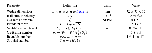
Figure 1. (a) A schematic of the experimental flow facility with gas ventilation line shown in red: A, pressure vessel; B, valve; C, voltage regulated mass flow controller; D, three-way valve. The yellow region indicates the field of view (FOV) for high-speed optical imaging, while the grey (FOV-1) and blue (FOV-2) regions indicate the FOV of X-ray imaging. The pressure is measured at $P_{0}, P_{1}$
and
$P_{0}, P_{1}$
and $P_{c}$
. (b) A schematic of the wedge with ventilation holes. (c) A schematic of the ventilated cavity. Note that the red arrow shows the direction of the gas flow, while the blue arrow shows the direction of the bulk flow.
$P_{c}$
. (b) A schematic of the wedge with ventilation holes. (c) A schematic of the ventilated cavity. Note that the red arrow shows the direction of the gas flow, while the blue arrow shows the direction of the bulk flow.
The ventilated partial cavity was generated behind a two-dimensional wedge by injecting non-condensable gas in its wake as shown in figure 1(c). The wedge had a height ( $H$
) of 19 mm and an angle of 15
$H$
) of 19 mm and an angle of 15 $^{\circ }$
, and was seal-secured tightly by the test-section windows, resulting in a blockage (
$^{\circ }$
, and was seal-secured tightly by the test-section windows, resulting in a blockage ( $\xi$
) of 25 %. The wedge had an internal borehole leading to multiple ventilation ports of 1 mm diameter each on the wedge base, as detailed in Wu et al. (Reference Wu, Deijlen, Bhatt, Ganesh and Ceccio2021). The borehole was connected to the external compressed air supply via pneumatic fittings as shown in figure 1(b). The gas ventilation line is schematically illustrated in figure 1(a). The non-condensable gas was fed through a pressure vessel to maintain the required stagnation pressure (
$\xi$
) of 25 %. The wedge had an internal borehole leading to multiple ventilation ports of 1 mm diameter each on the wedge base, as detailed in Wu et al. (Reference Wu, Deijlen, Bhatt, Ganesh and Ceccio2021). The borehole was connected to the external compressed air supply via pneumatic fittings as shown in figure 1(b). The gas ventilation line is schematically illustrated in figure 1(a). The non-condensable gas was fed through a pressure vessel to maintain the required stagnation pressure ( $\sim$
400 kPa) to mitigate choking in the ventilation lines. The mass flow rate (
$\sim$
400 kPa) to mitigate choking in the ventilation lines. The mass flow rate ( $\dot {Q}_{in}$
) was controlled using two flow controllers: Omega FMA series 0–15 and 0–50 standard litres per minute (SLPM). The gas injection rate was measured in SLPM due to a lack of pressure measurements near the injection ports. The injected gas flow rate was expressed as the non-dimensional ventilation coefficient
$\dot {Q}_{in}$
) was controlled using two flow controllers: Omega FMA series 0–15 and 0–50 standard litres per minute (SLPM). The gas injection rate was measured in SLPM due to a lack of pressure measurements near the injection ports. The injected gas flow rate was expressed as the non-dimensional ventilation coefficient $C_{qs}$
(see table 1 for definition) and was varied from 0.02 to 0.12 for a given base pressure. The pressure inside the cavity (
$C_{qs}$
(see table 1 for definition) and was varied from 0.02 to 0.12 for a given base pressure. The pressure inside the cavity ( $P_{c}$
) was measured from the side window of the test section at
$P_{c}$
) was measured from the side window of the test section at $x \approx 1H$
, along the wedge centreline, using an Omega Engineering PX409030DWU10V, 0–208 kPa transducer (see figure 1
a). The measured cavity pressure, incoming pressure (
$x \approx 1H$
, along the wedge centreline, using an Omega Engineering PX409030DWU10V, 0–208 kPa transducer (see figure 1
a). The measured cavity pressure, incoming pressure ( $P_{0}$
) and dynamic pressure of the incoming flow (
$P_{0}$
) and dynamic pressure of the incoming flow ( $ ({1}/{2})\rho U_{0}^2$
) were used to define the cavitation number expressed as
$ ({1}/{2})\rho U_{0}^2$
) were used to define the cavitation number expressed as $\sigma _{c}$
(see table 1 for definition). Note that cavitation number is used extensively in natural cavitating flows to indicate the closeness of cavity pressure to the vapour pressure (Brennen Reference Brennen1995).
$\sigma _{c}$
(see table 1 for definition). Note that cavitation number is used extensively in natural cavitating flows to indicate the closeness of cavity pressure to the vapour pressure (Brennen Reference Brennen1995).
2.2. Flow visualisation
Visual observation and qualitative analyses of ventilated partial cavities were performed via front-illuminated high-speed cinematography using a single Phantom Cinemag 2 v710 camera placed perpendicular to the FOV. The FOV was centred along the test-section axis and spans 13.6 $H$
$H$ $\times$
8.4
$\times$
8.4 $H$
in the
$H$
in the $x{-}y$
plane with the origin (
$x{-}y$
plane with the origin ( $x$
,
$x$
, $y$
,
$y$
, $z$
= 0) defined at the centre of the wedge base. See the yellow region in figure 1(a) for the FOV. In a separate set of experiments, auxiliary high-speed visualisations were also performed to image a top-view of the cavity in the
$z$
= 0) defined at the centre of the wedge base. See the yellow region in figure 1(a) for the FOV. In a separate set of experiments, auxiliary high-speed visualisations were also performed to image a top-view of the cavity in the $x{-}z$
plane with similar settings. The camera was equipped with a 105 mm Nikkor lens set to
$x{-}z$
plane with similar settings. The camera was equipped with a 105 mm Nikkor lens set to $f^{\#}$
= 5.6 to allow sufficient contrast in images. The images were acquired at 500–2000 Hz for
$f^{\#}$
= 5.6 to allow sufficient contrast in images. The images were acquired at 500–2000 Hz for $\sim$
11–44 s, depending on the nature of the experiment. Time-resolved, spanwise-averaged void fraction fields of ventilated cavities were measured using a high-speed two-dimensional X-ray densitometry system described in detail in Mäkiharju et al. (Reference Mäkiharju, Gabillet, Paik, Chang, Perlin and Ceccio2013b
). The current and the voltage of the X-ray source were set to 140 mA and 60 kV, respectively, resulting in a measurement time of 1.6 s. The FOV-1, corresponding to X-ray densitometry, spanned 8.2
$\sim$
11–44 s, depending on the nature of the experiment. Time-resolved, spanwise-averaged void fraction fields of ventilated cavities were measured using a high-speed two-dimensional X-ray densitometry system described in detail in Mäkiharju et al. (Reference Mäkiharju, Gabillet, Paik, Chang, Perlin and Ceccio2013b
). The current and the voltage of the X-ray source were set to 140 mA and 60 kV, respectively, resulting in a measurement time of 1.6 s. The FOV-1, corresponding to X-ray densitometry, spanned 8.2 $H$
$H$ $\times$
4
$\times$
4 $H$
in the
$H$
in the $x{-}y$
plane (see grey region in figure 1
a). An obstruction in the line of sight of X-rays resulted in a small disc-shaped, non-physical artefact in the void fraction fields, located at
$x{-}y$
plane (see grey region in figure 1
a). An obstruction in the line of sight of X-rays resulted in a small disc-shaped, non-physical artefact in the void fraction fields, located at $x/H \approx$
0.78,
$x/H \approx$
0.78, $y/H \approx$
–0.52: see, for instance, the black disc in figure 4(c). In order to make an estimate of the uncertainty level in void fraction measurements, we examined the void fractions in the ambient liquid. This region contains pure liquid with gas fraction,
$y/H \approx$
–0.52: see, for instance, the black disc in figure 4(c). In order to make an estimate of the uncertainty level in void fraction measurements, we examined the void fractions in the ambient liquid. This region contains pure liquid with gas fraction, $\alpha = 0$
. The measured instantaneous void fraction in the pure liquid phase is
$\alpha = 0$
. The measured instantaneous void fraction in the pure liquid phase is ${\lt}0.02 \pm 0.02$
, while in the pure gas phase, it is
${\lt}0.02 \pm 0.02$
, while in the pure gas phase, it is ${\gt}0.97 \pm 0.02$
. A more elaborate discussion on uncertainty and its sources is detailed in Mäkiharju et al. (Reference Mäkiharju, Gabillet, Paik, Chang, Perlin and Ceccio2013b
). The instantaneous void fractions were estimated with a spatial resolution of 0.16 mm (
${\gt}0.97 \pm 0.02$
. A more elaborate discussion on uncertainty and its sources is detailed in Mäkiharju et al. (Reference Mäkiharju, Gabillet, Paik, Chang, Perlin and Ceccio2013b
). The instantaneous void fractions were estimated with a spatial resolution of 0.16 mm ( $0.0084H$
) and a temporal resolution of 0.001 s. For long cavities with closure in the region beyond the X-ray measurement domain (FOV-1), only qualitative X-ray visualisation (i.e. no quantitative void fraction field measurements) could be performed from
$0.0084H$
) and a temporal resolution of 0.001 s. For long cavities with closure in the region beyond the X-ray measurement domain (FOV-1), only qualitative X-ray visualisation (i.e. no quantitative void fraction field measurements) could be performed from $x$
= 14
$x$
= 14 $H$
to 22
$H$
to 22 $H$
. This alternate FOV is shown by the blue region marked ‘FOV-2’ in figure 1(a). The thicker and denser polyvinyl chloride (PVC) walls of the test facility led to a substantial reduction in signal-to-noise ratio (SNR) and an increase in measurement uncertainty precluding the quantification of void fractions; the measured void fraction of pure liquid in this configuration is approximately 0.097
$H$
. This alternate FOV is shown by the blue region marked ‘FOV-2’ in figure 1(a). The thicker and denser polyvinyl chloride (PVC) walls of the test facility led to a substantial reduction in signal-to-noise ratio (SNR) and an increase in measurement uncertainty precluding the quantification of void fractions; the measured void fraction of pure liquid in this configuration is approximately 0.097 $\pm$
0.17. Hence, X-ray measurements in this region were used only for qualitative visualisation of closures region of long cavities (supercavities at high
$\pm$
0.17. Hence, X-ray measurements in this region were used only for qualitative visualisation of closures region of long cavities (supercavities at high $\textit{Fr}$
). The image acquisition (high-speed photography and X-ray imaging) was time-synchronised with gas ventilation input (
$\textit{Fr}$
). The image acquisition (high-speed photography and X-ray imaging) was time-synchronised with gas ventilation input ( $\dot {Q}$
) and pressure transducers (
$\dot {Q}$
) and pressure transducers ( $P_{1}$
,
$P_{1}$
, $P_{0}$
,
$P_{0}$
, $P_{c}$
) using a digital pulse generator (DG535, Stanford Research Systems).
$P_{c}$
) using a digital pulse generator (DG535, Stanford Research Systems).
2.3. Experimental procedure
The experiments were performed for a range of $U_{0}$
(
$U_{0}$
( $\textit{Fr}$
) and over 100 different ventilation inputs (
$\textit{Fr}$
) and over 100 different ventilation inputs ( $C_{qs}$
). Since the aim of this study was also to examine the formation dynamics of a ventilated cavity, we performed two different types of experiments. In the first set of experiments, the gas was injected from no injection (
$C_{qs}$
). Since the aim of this study was also to examine the formation dynamics of a ventilated cavity, we performed two different types of experiments. In the first set of experiments, the gas was injected from no injection ( $C_{qs} \sim$
0) to the desired
$C_{qs} \sim$
0) to the desired $C_{qs}$
with a prescribed error function such that
$C_{qs}$
with a prescribed error function such that ${\rm d}{C_{qs}}/{\rm d}t \gt 0$
or
${\rm d}{C_{qs}}/{\rm d}t \gt 0$
or $\dot {C}_{qs}\gt 0$
. This ventilation strategy is referred to as ‘L-H’, as the ventilation is increased from zero to a given
$\dot {C}_{qs}\gt 0$
. This ventilation strategy is referred to as ‘L-H’, as the ventilation is increased from zero to a given $C_{qs}$
(see red profile in figure 2) in approximately 5 s and kept constant for at least 10 s depending on the nature of the experiment. In the second set of experiments, a fully developed supercavity was used as an initial condition, and the gas injection rate was reduced with an error function to achieve the desired
$C_{qs}$
(see red profile in figure 2) in approximately 5 s and kept constant for at least 10 s depending on the nature of the experiment. In the second set of experiments, a fully developed supercavity was used as an initial condition, and the gas injection rate was reduced with an error function to achieve the desired $C_{qs}$
, i.e.
$C_{qs}$
, i.e. $ \dot {C}_{qs}\lt 0$
(see black profile in figure 2). This ventilation strategy is referred to as ‘H-L’ as the ventilation rate is reduced. High
$ \dot {C}_{qs}\lt 0$
(see black profile in figure 2). This ventilation strategy is referred to as ‘H-L’ as the ventilation rate is reduced. High $C_{qs}$
were maintained for at least 5 s to ensure that the supercavity closure is fully developed before reducing it to the final low
$C_{qs}$
were maintained for at least 5 s to ensure that the supercavity closure is fully developed before reducing it to the final low $C_{qs}$
, which is kept constant for at least 15 s. Thus, for both strategies, upon establishing a cavity, measurements were performed after waiting for sufficient time to ensure that the cavity length did not change. See the grey region in figure 2. Note that the effect of the rate of increase of
$C_{qs}$
, which is kept constant for at least 15 s. Thus, for both strategies, upon establishing a cavity, measurements were performed after waiting for sufficient time to ensure that the cavity length did not change. See the grey region in figure 2. Note that the effect of the rate of increase of $C_{qs}$
is beyond the scope of the current study. The ventilation was increased/decreased smoothly with an error function to mitigate the sharp overshoot in
$C_{qs}$
is beyond the scope of the current study. The ventilation was increased/decreased smoothly with an error function to mitigate the sharp overshoot in $\dot {Q}_{in}$
inherent to the first-order step response of the mass flow controller. This allowed precise control of the volume of gas injected in the flow. After each measurement, the flow loop was carefully deaerated to ensure that there was no incoming free gas. The flow parameters of the experimental campaign are listed in table 1.
$\dot {Q}_{in}$
inherent to the first-order step response of the mass flow controller. This allowed precise control of the volume of gas injected in the flow. After each measurement, the flow loop was carefully deaerated to ensure that there was no incoming free gas. The flow parameters of the experimental campaign are listed in table 1.
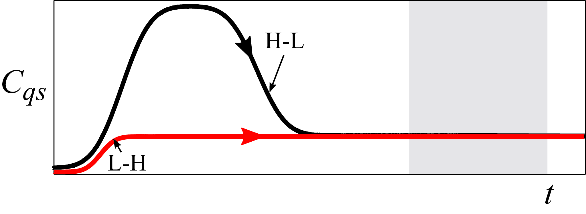
Figure 2. Schematic gas injection profiles in time: red indicates a typical L-H profile, while black indicates a typical H-L profile. The grey region denotes the measurement time interval.
3. Characteristics of ventilated cavities
The defining characteristics of ventilated cavities classified based on the closure region are discussed in this section along with their occurrence on a regime map. In addition, cavities observed during the transition from one type to another, designated as transitional cavities, are discussed in § 4.
3.1. Cavity classification
Four types of ventilated cavities are identified based on the cavity closure region for the range of $C_{qs}$
and
$C_{qs}$
and $\textit{Fr}$
considered. They are classified as foamy cavities (FCs), twin-branched cavities (TBCs), re-entrant jet cavities (REJCs) and long cavities (LCs). The classification is based on the visual interpretation of optical images and X-ray-based void fraction fields.
$\textit{Fr}$
considered. They are classified as foamy cavities (FCs), twin-branched cavities (TBCs), re-entrant jet cavities (REJCs) and long cavities (LCs). The classification is based on the visual interpretation of optical images and X-ray-based void fraction fields.
3.1.1. Foamy cavities
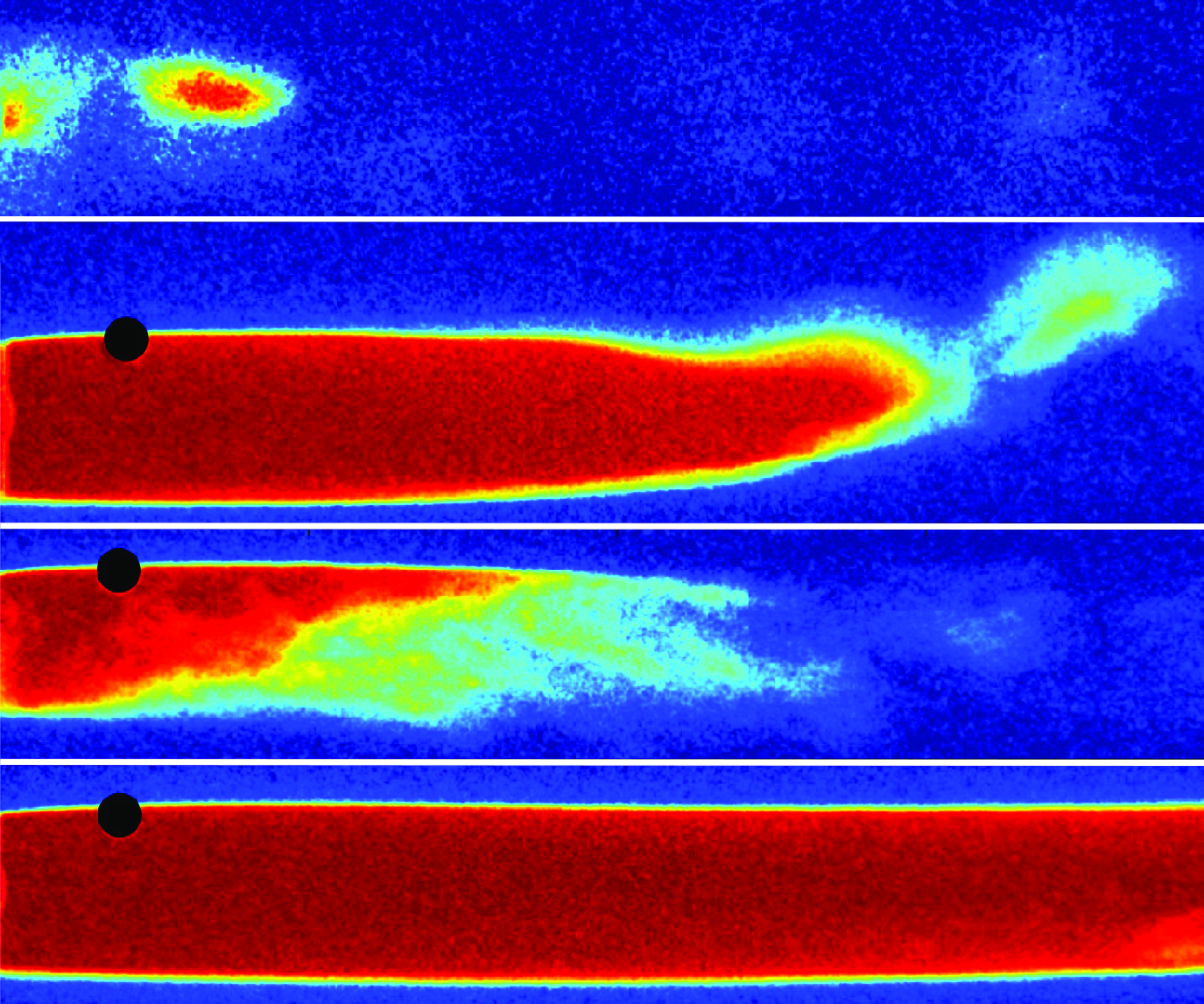
These cavities were observed for $C_{qs}\lt 0.043$
and all the considered
$C_{qs}\lt 0.043$
and all the considered $\textit{Fr}$
(
$\textit{Fr}$
( $\sim$
2–13.9). Figure 3(a) shows a snapshot from high-speed imaging of an FC observed at
$\sim$
2–13.9). Figure 3(a) shows a snapshot from high-speed imaging of an FC observed at $\textit{Fr}=13.9$
and
$\textit{Fr}=13.9$
and $C_{qs}$
= 0.0205. Figure 3(b) shows the corresponding instantaneous void fraction field measured using time-resolved X-ray densitometry in a separate experiment. The cavity is characterised by the presence of injected gas as dispersed gas bubbles in the near wake of the wedge. Foamy cavities do not have a well-defined closure region and are characterised by gas ejection via vortex shedding in the wake of the wedge. Visual observation reveals that cavities are nominally two-dimensional in the near-wake region similar to natural cavities reported by Wu et al. (Reference Wu, Deijlen, Bhatt, Ganesh and Ceccio2021) in the same geometry. Such cavities have also been observed in other cavitator geometries such as backward-facing steps (Qin et al. Reference Qin, Wu, Wu and Hong2019), disc cavitators (Karn et al. Reference Karn, Arndt and Hong2016) and three-dimensional fences (Barbaca et al. Reference Barbaca, Pearce and Brandner2017). In the near-wake region, optical imaging shows the presence of large gas content. However, X-ray visualisation clarifies that this apparent gas content is a mere imaging artefact, arising from the glaring caused by reflection (specular) due to the test section and surrounding gas. This highlights the advantages of radiation-based flow visualisation techniques in studying bubbly flows complementary to optical imaging.
$C_{qs}$
= 0.0205. Figure 3(b) shows the corresponding instantaneous void fraction field measured using time-resolved X-ray densitometry in a separate experiment. The cavity is characterised by the presence of injected gas as dispersed gas bubbles in the near wake of the wedge. Foamy cavities do not have a well-defined closure region and are characterised by gas ejection via vortex shedding in the wake of the wedge. Visual observation reveals that cavities are nominally two-dimensional in the near-wake region similar to natural cavities reported by Wu et al. (Reference Wu, Deijlen, Bhatt, Ganesh and Ceccio2021) in the same geometry. Such cavities have also been observed in other cavitator geometries such as backward-facing steps (Qin et al. Reference Qin, Wu, Wu and Hong2019), disc cavitators (Karn et al. Reference Karn, Arndt and Hong2016) and three-dimensional fences (Barbaca et al. Reference Barbaca, Pearce and Brandner2017). In the near-wake region, optical imaging shows the presence of large gas content. However, X-ray visualisation clarifies that this apparent gas content is a mere imaging artefact, arising from the glaring caused by reflection (specular) due to the test section and surrounding gas. This highlights the advantages of radiation-based flow visualisation techniques in studying bubbly flows complementary to optical imaging.
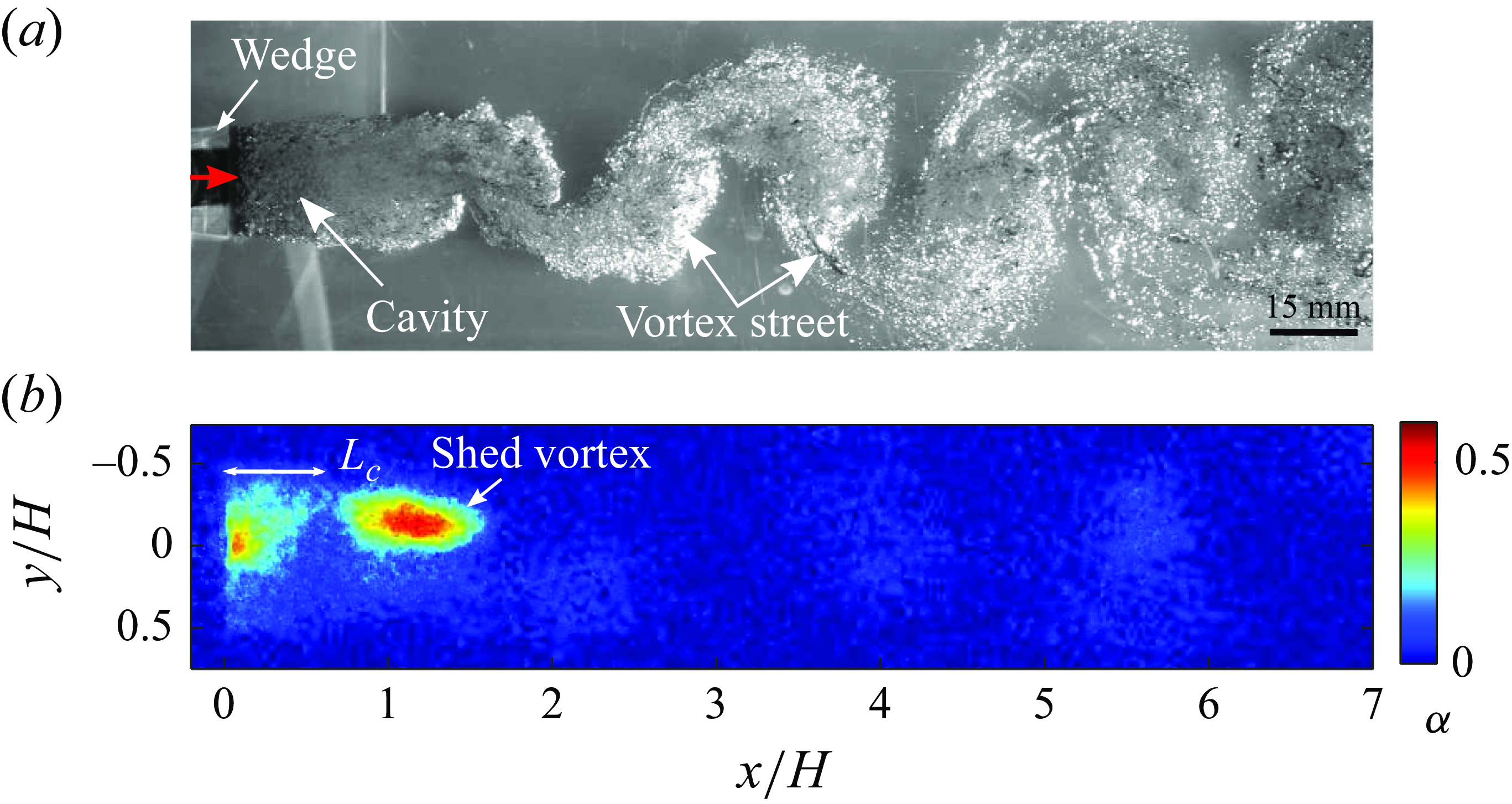
Figure 3. A side view ( $x{-}y$
) of an FC at
$x{-}y$
) of an FC at $\textit{Fr}=13.9$
,
$\textit{Fr}=13.9$
, $C_{qs}$
= 0.0205. (a) A snapshot from high-speed optical imaging. The red arrow shows the direction of the ventilation and the bulk flow. (b) A snapshot from highspeed X-ray imaging at the same flow condition. Here,
$C_{qs}$
= 0.0205. (a) A snapshot from high-speed optical imaging. The red arrow shows the direction of the ventilation and the bulk flow. (b) A snapshot from highspeed X-ray imaging at the same flow condition. Here, $L_c$
indicates cavity length. The geometric magnification in X-ray images is not identical to optical images due to the difference in FOVs. The same holds true for figures 4, 5 and 6 presented later. The colourbar shows spanwise-averaged void fractions.
$L_c$
indicates cavity length. The geometric magnification in X-ray images is not identical to optical images due to the difference in FOVs. The same holds true for figures 4, 5 and 6 presented later. The colourbar shows spanwise-averaged void fractions.
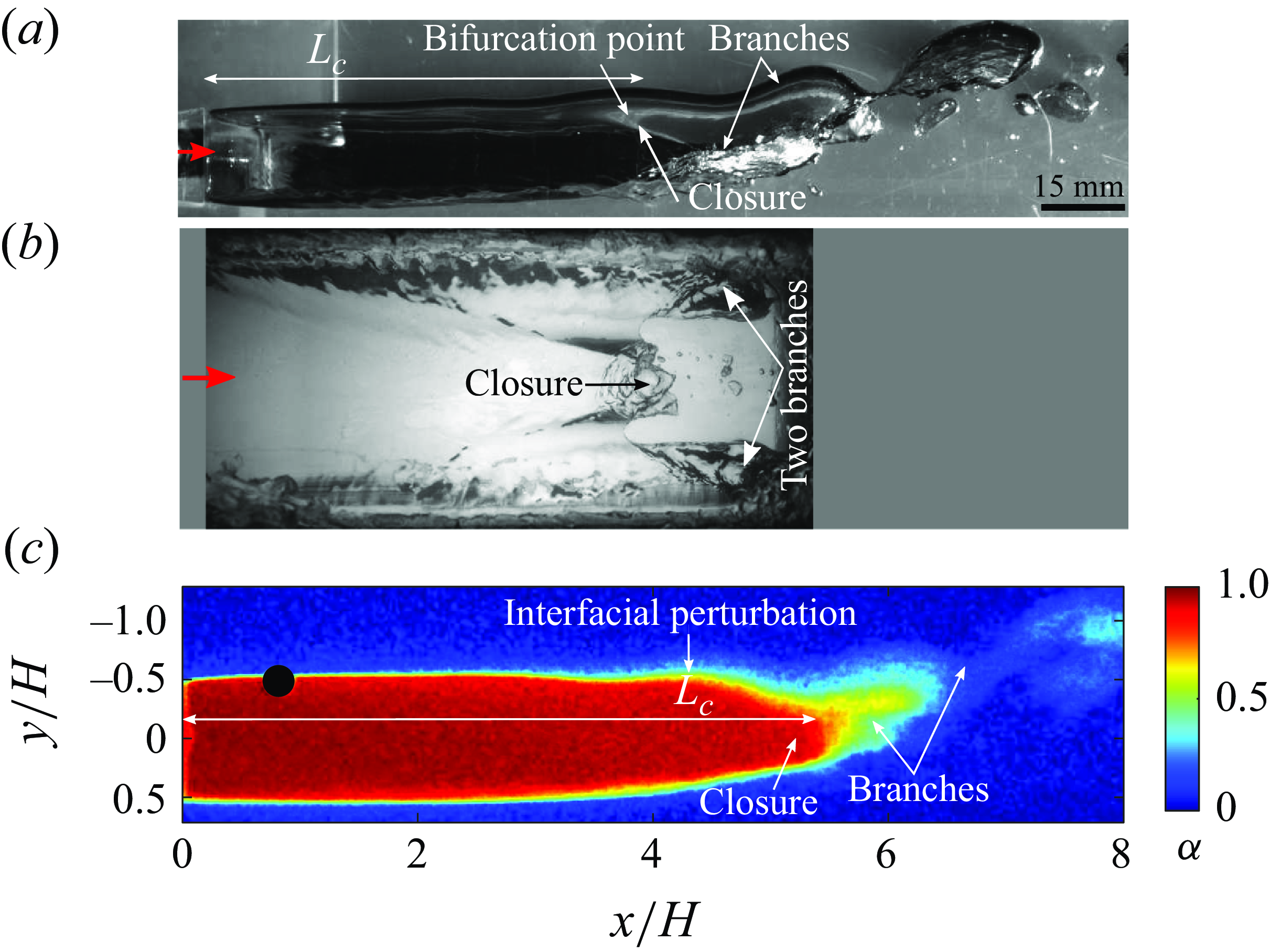
Figure 4. Twin-branched cavity at $\textit{Fr}$
= 2.08,
$\textit{Fr}$
= 2.08, $C_{qs}$
= 0.058. (a) A snapshot from high-speed optical imaging in the
$C_{qs}$
= 0.058. (a) A snapshot from high-speed optical imaging in the $x{-}y$
plane. (b) The top view (
$x{-}y$
plane. (b) The top view ( $x{-}z$
plane), dark-grey masked region indicates lack of optical access inherent to test section. (c) The instantaneous void fraction field of a TBC in the
$x{-}z$
plane), dark-grey masked region indicates lack of optical access inherent to test section. (c) The instantaneous void fraction field of a TBC in the $x{-}y$
plane.
$x{-}y$
plane.
3.1.2. Twin-branched cavities
For $2.08 \leqslant Fr \leqslant 4.17$
and
$2.08 \leqslant Fr \leqslant 4.17$
and $C_{qs} \gt 0.043$
, an attached cavity with a weak re-entrant flow near its closure (see flow structure near region marked ‘closure’ in figure 4
b) and two prominent branches (legs) alongside the walls are observed as shown in figure 4. A prominent travelling perturbation is seen on the upper cavity interface (see figure 4
c). Twin-branched cavities are filled with gas (
$C_{qs} \gt 0.043$
, an attached cavity with a weak re-entrant flow near its closure (see flow structure near region marked ‘closure’ in figure 4
b) and two prominent branches (legs) alongside the walls are observed as shown in figure 4. A prominent travelling perturbation is seen on the upper cavity interface (see figure 4
c). Twin-branched cavities are filled with gas ( $\alpha \sim 1$
) as seen in X-ray-based void fraction measurements shown in figure 4(c). The cavities at these flow conditions exhibit a prominent camber due to buoyancy effects. The resulting upward curvature of the upper cavity interface leads to lift generation and formation of trailing vortices (Semenenko Reference Semenenko2001), observed as two branches (see figure 4
b). Similar cavities were observed behind a two-dimensional wall-bounded cavitator by Barbaca et al. (Reference Barbaca, Pearce and Brandner2017) and Qin et al. (Reference Qin, Wu, Wu and Hong2019). These cavities show a close resemblance to the twin-vortex-tube-type ventilated cavities reported in three-dimensional axisymmetric cavitators (Semenenko Reference Semenenko2001; Kawakami & Arndt Reference Kawakami and Arndt2011). With an increase in
$\alpha \sim 1$
) as seen in X-ray-based void fraction measurements shown in figure 4(c). The cavities at these flow conditions exhibit a prominent camber due to buoyancy effects. The resulting upward curvature of the upper cavity interface leads to lift generation and formation of trailing vortices (Semenenko Reference Semenenko2001), observed as two branches (see figure 4
b). Similar cavities were observed behind a two-dimensional wall-bounded cavitator by Barbaca et al. (Reference Barbaca, Pearce and Brandner2017) and Qin et al. (Reference Qin, Wu, Wu and Hong2019). These cavities show a close resemblance to the twin-vortex-tube-type ventilated cavities reported in three-dimensional axisymmetric cavitators (Semenenko Reference Semenenko2001; Kawakami & Arndt Reference Kawakami and Arndt2011). With an increase in $\textit{Fr}$
, the upward camber of the cavity decreases due to the increased effect of fluid inertia relative to gravity. Twin-branched cavities are nominally two-dimensional along their axis until the bifurcation point slightly upstream of the closure where the cavity is divided into two branches, resulting in three-dimensional cavity closure, as shown in figure 4. The body and the branches of the supercavity are distinguished in X-ray visualisations by a high-void-fraction region (
$\textit{Fr}$
, the upward camber of the cavity decreases due to the increased effect of fluid inertia relative to gravity. Twin-branched cavities are nominally two-dimensional along their axis until the bifurcation point slightly upstream of the closure where the cavity is divided into two branches, resulting in three-dimensional cavity closure, as shown in figure 4. The body and the branches of the supercavity are distinguished in X-ray visualisations by a high-void-fraction region ( $\alpha \sim$
0.90) spanning
$\alpha \sim$
0.90) spanning $x \simeq 0{-}5H$
and a low-void-fraction region (
$x \simeq 0{-}5H$
and a low-void-fraction region ( $\alpha \sim$
0.4–0.6) spanning
$\alpha \sim$
0.4–0.6) spanning $x \simeq 5{-}6.5H$
, respectively. It is imperative to note that gas-filled branches exhibit low void fraction due to the spanwise-averaging of the three-dimensional flow features inherent to 2-D densitometry, discussed in Gawandalkar (Reference Gawandalkar2024). Hence, X-ray-based void fraction measurements near the closure region of TBCs is qualitative, aiding in flow visualisation, not a quantitative measurement of void fraction and gas ejection.
$x \simeq 5{-}6.5H$
, respectively. It is imperative to note that gas-filled branches exhibit low void fraction due to the spanwise-averaging of the three-dimensional flow features inherent to 2-D densitometry, discussed in Gawandalkar (Reference Gawandalkar2024). Hence, X-ray-based void fraction measurements near the closure region of TBCs is qualitative, aiding in flow visualisation, not a quantitative measurement of void fraction and gas ejection.
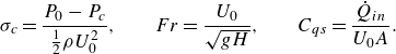
3.1.3. Re-entrant jet cavities
A third type of cavity, characterised by a strong re-entrant flow originating at the cavity closure and spanning the entire cavity length, was observed at higher flow velocity ( $5.79 \leqslant Fr \leqslant 13.9$
) and intermediate ventilation rate (
$5.79 \leqslant Fr \leqslant 13.9$
) and intermediate ventilation rate ( $0.045 \leqslant C_{qs} \leqslant 0.065$
). These are termed REJCs and an example is shown in figure 5. The REJCs are marked by Von Kármán vortex streets downstream of the closure. It should be noted that the presence of a liquid re-entrant flow is in the context of the cavity topology resulting from the accumulation of gas near the top interface. This results in an altered interaction of the shear layers when compared with a non-cavitating wake flow. The gas in the cavity can be identified by a relatively clear part (see also the labelled region in figure 5
a), while the re-entrant flow is seen by the frothy liquid inside the cavity (see labelled region in figure 5
a). Gas ejection caused by the liquid flow downstream of the identified closure region is shown in figure 5(a). The measured density field shows that the re-entering liquid flow is confined to the lower half of the cavity, while the gas accumulates in the upper half (see figure 5
b). The REJCs are nominally two-dimensional with a highly frothy and turbulent cavity closure. These cavities are slightly asymmetric about the wedge centreline (
$0.045 \leqslant C_{qs} \leqslant 0.065$
). These are termed REJCs and an example is shown in figure 5. The REJCs are marked by Von Kármán vortex streets downstream of the closure. It should be noted that the presence of a liquid re-entrant flow is in the context of the cavity topology resulting from the accumulation of gas near the top interface. This results in an altered interaction of the shear layers when compared with a non-cavitating wake flow. The gas in the cavity can be identified by a relatively clear part (see also the labelled region in figure 5
a), while the re-entrant flow is seen by the frothy liquid inside the cavity (see labelled region in figure 5
a). Gas ejection caused by the liquid flow downstream of the identified closure region is shown in figure 5(a). The measured density field shows that the re-entering liquid flow is confined to the lower half of the cavity, while the gas accumulates in the upper half (see figure 5
b). The REJCs are nominally two-dimensional with a highly frothy and turbulent cavity closure. These cavities are slightly asymmetric about the wedge centreline ( $y$
= 0). Despite this asymmetry, REJC shapes do not have a strong dependence on
$y$
= 0). Despite this asymmetry, REJC shapes do not have a strong dependence on $\textit{Fr}$
. Such cavities resemble those reported by Kawakami & Arndt (Reference Kawakami and Arndt2011); Barbaca et al. (Reference Barbaca, Pearce and Brandner2017) behind a three-dimensional cavitator. However, these cavities are different from REJCs reported by Semenenko (Reference Semenenko2001); Karn et al. (Reference Karn, Arndt and Hong2016), where the re-entrant jet was substantially shorter than the cavity length and was confined to the cavity closure region.
$\textit{Fr}$
. Such cavities resemble those reported by Kawakami & Arndt (Reference Kawakami and Arndt2011); Barbaca et al. (Reference Barbaca, Pearce and Brandner2017) behind a three-dimensional cavitator. However, these cavities are different from REJCs reported by Semenenko (Reference Semenenko2001); Karn et al. (Reference Karn, Arndt and Hong2016), where the re-entrant jet was substantially shorter than the cavity length and was confined to the cavity closure region.
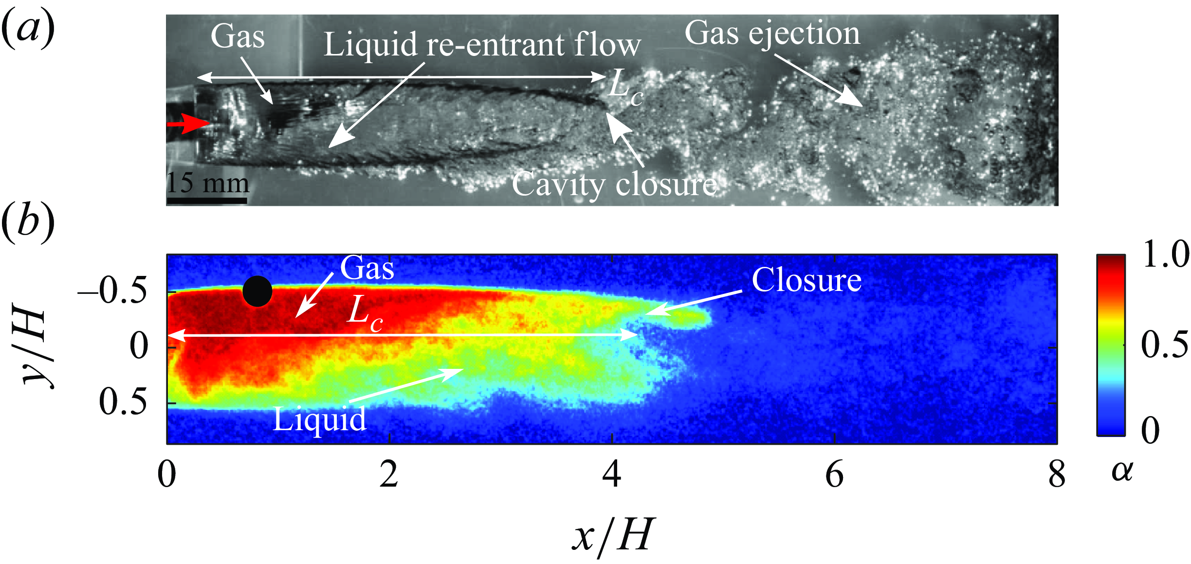
Figure 5. A side view ( $x{-}y$
) of an REJC at
$x{-}y$
) of an REJC at $\textit{Fr}$
= 5.79,
$\textit{Fr}$
= 5.79, $C_{qs}$
= 0.054: (a) optical imaging, (b) an instantaneous void fraction field.
$C_{qs}$
= 0.054: (a) optical imaging, (b) an instantaneous void fraction field.
3.1.4. Long cavities
Long cavities exist for $5.79 \leqslant Fr \leqslant 13.9$
and
$5.79 \leqslant Fr \leqslant 13.9$
and $C_{qs}\geqslant 0.07$
. The LCs span beyond the optical FOV (see figure 6). Thus, the complete cavity could not be visualised with high-speed imaging and the closure of the cavity could not be measured quantitatively using X-ray densitometry. However, qualitative X-ray-based visualisation was performed to study cavity closure dynamics. Typically, the length of these cavities is more than 12
$C_{qs}\geqslant 0.07$
. The LCs span beyond the optical FOV (see figure 6). Thus, the complete cavity could not be visualised with high-speed imaging and the closure of the cavity could not be measured quantitatively using X-ray densitometry. However, qualitative X-ray-based visualisation was performed to study cavity closure dynamics. Typically, the length of these cavities is more than 12 $H$
. The observable portion of these cavities was two-dimensional and filled with gas, as evident from the instantaneous void fraction distributions in figure 6(b). There is no observable effect of gravity on their shape. These cavities have small-scale instabilities on the cavity interface, as indicated in figure 6(a). Long cavities exhibit oscillations in the
$H$
. The observable portion of these cavities was two-dimensional and filled with gas, as evident from the instantaneous void fraction distributions in figure 6(b). There is no observable effect of gravity on their shape. These cavities have small-scale instabilities on the cavity interface, as indicated in figure 6(a). Long cavities exhibit oscillations in the $x{-}y$
plane similar to PCs reported by Silberman & Song (Reference Silberman and Song1961), Michel (Reference Michel1984), Skidmore (Reference Skidmore2016).
$x{-}y$
plane similar to PCs reported by Silberman & Song (Reference Silberman and Song1961), Michel (Reference Michel1984), Skidmore (Reference Skidmore2016).
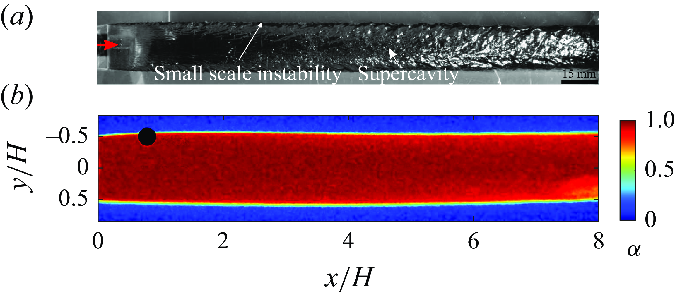
Figure 6. The side view ( $x{-}y$
) of an LC at
$x{-}y$
) of an LC at $\textit{Fr}$
= 10.42,
$\textit{Fr}$
= 10.42, $C_{qs}$
= 0.090.
$C_{qs}$
= 0.090.
3.2. Cavity closure regime map
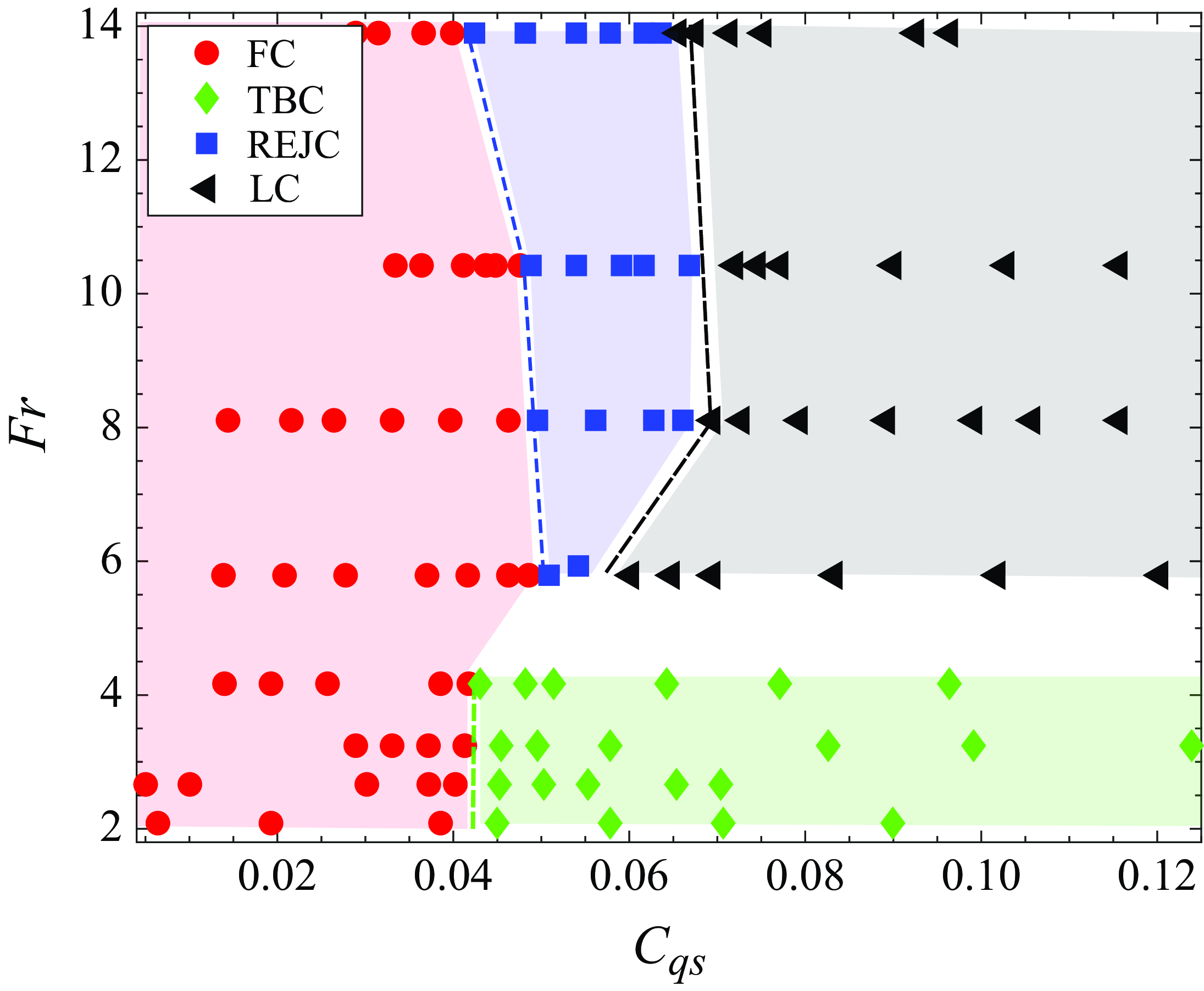
Figure 7. The regime map ( $\textit{Fr}$
–
$\textit{Fr}$
– $C_{qs}$
) shows different types of observed ventilated partial/supercavities indicated by different colours: red, FC; green, TBC blue, REJC black, LC. The dashed lines show the demarcation from one regime to another, i.e. green dashed line,
$C_{qs}$
) shows different types of observed ventilated partial/supercavities indicated by different colours: red, FC; green, TBC blue, REJC black, LC. The dashed lines show the demarcation from one regime to another, i.e. green dashed line, $C^{tr}_{qs,fc-tbc}$
; blue dashed line,
$C^{tr}_{qs,fc-tbc}$
; blue dashed line, $C^{tr}_{qs, fc-rejc}$
; black dashed line,
$C^{tr}_{qs, fc-rejc}$
; black dashed line, $C^{tr}_{qs, rejc-lc}$
.
$C^{tr}_{qs, rejc-lc}$
.
The observed cavity closure types and transition regions between them are identified on a regime map defined by the Froude number ( $\textit{Fr}$
) and ventilation coefficient (
$\textit{Fr}$
) and ventilation coefficient ( $C_{qs}$
) as shown in figure 7. The regime map is specific to the 2-D wedges as the exact regime map is dependent on the cavitator geometry, shown previously by Karn et al. (Reference Karn, Arndt and Hong2016), Qin et al. (Reference Qin, Wu, Wu and Hong2019). However, similar trends in regimes can be expected for other bluff body cavitators. The regime map was generated by fixing
$C_{qs}$
) as shown in figure 7. The regime map is specific to the 2-D wedges as the exact regime map is dependent on the cavitator geometry, shown previously by Karn et al. (Reference Karn, Arndt and Hong2016), Qin et al. (Reference Qin, Wu, Wu and Hong2019). However, similar trends in regimes can be expected for other bluff body cavitators. The regime map was generated by fixing $U_{0}$
(
$U_{0}$
( $\textit{Fr}$
), followed by increasing the gas injection to achieve a
$\textit{Fr}$
), followed by increasing the gas injection to achieve a $C_{qs}$
following the L-H ventilation strategy explained in § 2.3 (red profile in figure 2). Note that every data point is an independent experiment, i.e. with a ventilation profile starting from
$C_{qs}$
following the L-H ventilation strategy explained in § 2.3 (red profile in figure 2). Note that every data point is an independent experiment, i.e. with a ventilation profile starting from $C_{qs}$
= 0. For
$C_{qs}$
= 0. For $\textit{Fr} \gtrsim 5$
, the effect of gas buoyancy was observed to be less pronounced, and thus cavity types observed for
$\textit{Fr} \gtrsim 5$
, the effect of gas buoyancy was observed to be less pronounced, and thus cavity types observed for $\textit{Fr} \lesssim 5$
and
$\textit{Fr} \lesssim 5$
and $\textit{Fr} \gtrsim 5$
were different. The FCs (red region) and TBCs (green region) were observed for
$\textit{Fr} \gtrsim 5$
were different. The FCs (red region) and TBCs (green region) were observed for $\textit{Fr} \lesssim 5$
, meaning the TBC is the only supercavity observed at low
$\textit{Fr} \lesssim 5$
, meaning the TBC is the only supercavity observed at low $\textit{Fr}$
. The FC (red region), REJC (blue region) and LC (grey region) were observed for
$\textit{Fr}$
. The FC (red region), REJC (blue region) and LC (grey region) were observed for $\textit{Fr} \gtrsim 5$
. Thus two types of supercavities were observed at high
$\textit{Fr} \gtrsim 5$
. Thus two types of supercavities were observed at high $\textit{Fr}$
, namely the REJC and LC. The transition between the regimes occurs at a critical Froude number of
$\textit{Fr}$
, namely the REJC and LC. The transition between the regimes occurs at a critical Froude number of $\sim$
5 and near the dashed lines shown in figure 7.
$\sim$
5 and near the dashed lines shown in figure 7.
3.3. Cavity pressure
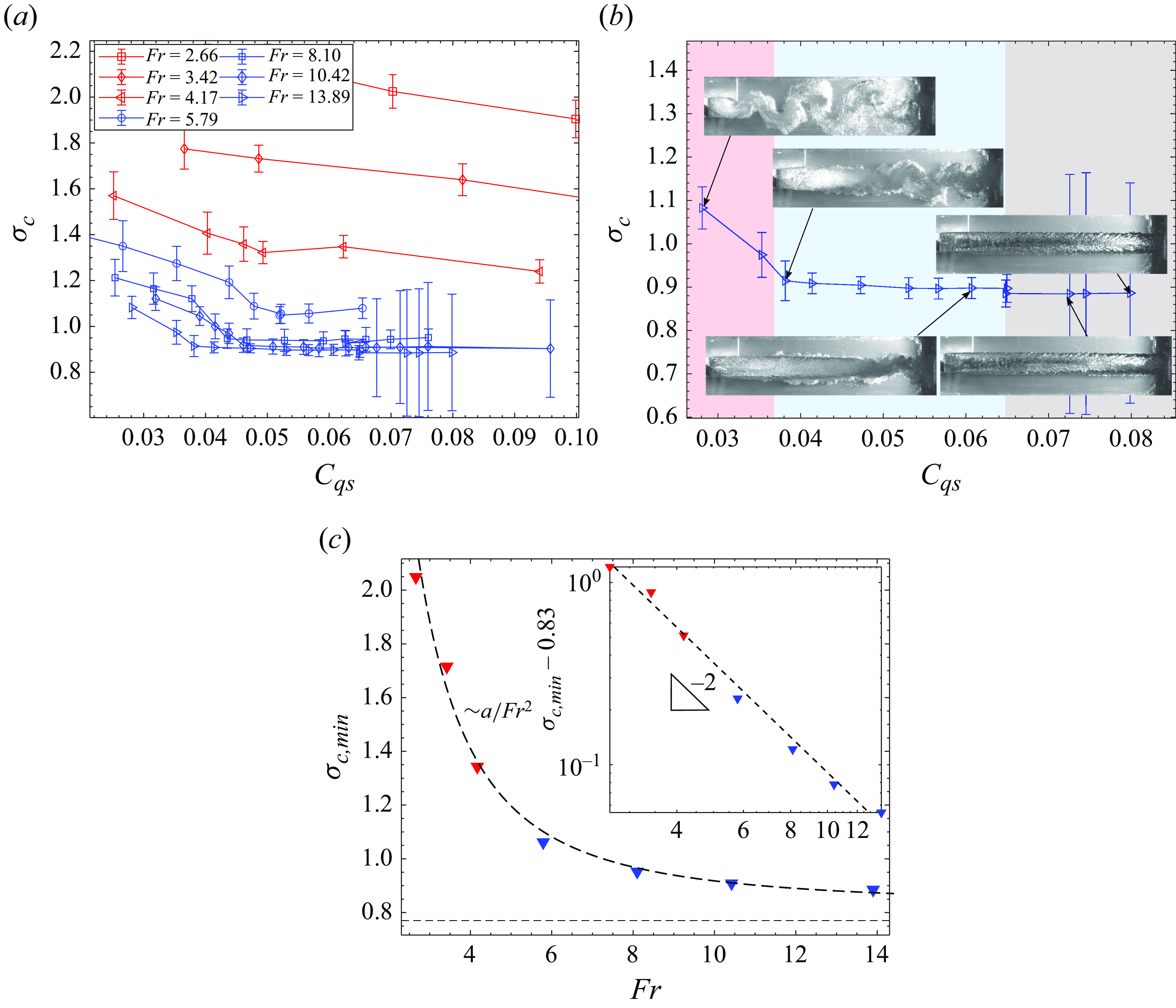
Figure 8. (a) Cavitation number ( $\sigma _{c}$
) based on measured cavity pressure as a function of ventilation coefficient (
$\sigma _{c}$
) based on measured cavity pressure as a function of ventilation coefficient ( $C_{qs}$
) at different
$C_{qs}$
) at different $\textit{Fr}$
(red markers show low-
$\textit{Fr}$
(red markers show low- $\textit{Fr}$
cases, while blue markers show high-
$\textit{Fr}$
cases, while blue markers show high- $\textit{Fr}$
cases). (b) Plot of
$\textit{Fr}$
cases). (b) Plot of $\sigma _{c}$
at
$\sigma _{c}$
at $\textit{Fr} = 13.89$
showing different ventilated cavity regimes. The red, blue and grey regions correspond to FC, REJC and LC closures, respectively. (c) Minimum
$\textit{Fr} = 13.89$
showing different ventilated cavity regimes. The red, blue and grey regions correspond to FC, REJC and LC closures, respectively. (c) Minimum $\sigma _{c}$
as a function of
$\sigma _{c}$
as a function of $\textit{Fr}$
. The black dashed curve shows a fit of the form
$\textit{Fr}$
. The black dashed curve shows a fit of the form $a\ Fr^{-2}$
, where a is a constant. The inset shows the same plot on an adjusted logarithmic scale. The grey dashed line shows
$a\ Fr^{-2}$
, where a is a constant. The inset shows the same plot on an adjusted logarithmic scale. The grey dashed line shows $\sigma _{c}=0.77$
computed with the Bernoulli equation.
$\sigma _{c}=0.77$
computed with the Bernoulli equation.
The pressure in the ventilated cavity is measured on the wedge centreline near the base, marked $P_{c}$
in figure 1(a). The measured pressures (
$P_{c}$
in figure 1(a). The measured pressures ( $P_{c}$
and
$P_{c}$
and $P_{0}$
) are used to compute the cavitation number or cavity underpressure coefficient (
$P_{0}$
) are used to compute the cavitation number or cavity underpressure coefficient ( $\sigma _{c}$
). Figure 8(a) shows the variation of
$\sigma _{c}$
). Figure 8(a) shows the variation of $\sigma _{c}$
with
$\sigma _{c}$
with $C_{qs}$
for a range of
$C_{qs}$
for a range of $\textit{Fr}$
considered in this study: the low-
$\textit{Fr}$
considered in this study: the low- $\textit{Fr}$
cases are shown by red markers, while the high-
$\textit{Fr}$
cases are shown by red markers, while the high- $\textit{Fr}$
cases are shown by blue markers. This demarcation in low versus high
$\textit{Fr}$
cases are shown by blue markers. This demarcation in low versus high $\textit{Fr}$
reflects the observations in the regime map (figure 7), which show a change in cavity closure type near
$\textit{Fr}$
reflects the observations in the regime map (figure 7), which show a change in cavity closure type near $\textit{Fr}$
= 5. At low
$\textit{Fr}$
= 5. At low $\textit{Fr}$
(
$\textit{Fr}$
( ${\approx}2.08{-}4.17$
), the cavity pressure could only be measured for TBCs, as FCs at low
${\approx}2.08{-}4.17$
), the cavity pressure could only be measured for TBCs, as FCs at low $\textit{Fr}$
were short, barring reliable measurement at the
$\textit{Fr}$
were short, barring reliable measurement at the $P_{c}$
location. Cavity underpressure coefficient (
$P_{c}$
location. Cavity underpressure coefficient ( $\sigma _c$
) is seen to be the highest at the lowest
$\sigma _c$
) is seen to be the highest at the lowest $\textit{Fr}$
consistent with the observations of Laali & Michel (Reference Laali and Michel1984). For FCs, the cavity pressure oscillates about a mean due to the periodic vortex street; however, for TBCs and REJCs, the cavity pressure remains fairly constant. For LCs, pressure oscillations are the largest due to the cavity pulsation in the
$\textit{Fr}$
consistent with the observations of Laali & Michel (Reference Laali and Michel1984). For FCs, the cavity pressure oscillates about a mean due to the periodic vortex street; however, for TBCs and REJCs, the cavity pressure remains fairly constant. For LCs, pressure oscillations are the largest due to the cavity pulsation in the $x{-}y$
plane. These pulsations are evident from the large standard deviations in
$x{-}y$
plane. These pulsations are evident from the large standard deviations in $\sigma _{c}$
for LCs as shown in figure 8(a,b). At lower
$\sigma _{c}$
for LCs as shown in figure 8(a,b). At lower $\textit{Fr}$
, once the TBC is formed,
$\textit{Fr}$
, once the TBC is formed, $\sigma _{c}$
does not change significantly for increasing
$\sigma _{c}$
does not change significantly for increasing $C_{qs}$
as shown in figure 8(a). Figure 8(b) shows the variation of
$C_{qs}$
as shown in figure 8(a). Figure 8(b) shows the variation of $\sigma _{c}$
with
$\sigma _{c}$
with $C_{qs}$
along with flow visualisations for a fixed Froude number (
$C_{qs}$
along with flow visualisations for a fixed Froude number ( $\textit{Fr} = 13.89$
):
$\textit{Fr} = 13.89$
): $\sigma _{c}$
decreases with an increase in ventilation (
$\sigma _{c}$
decreases with an increase in ventilation ( $C_{qs}$
) in the FC regime. With a further increase in
$C_{qs}$
) in the FC regime. With a further increase in $C_{qs}$
,
$C_{qs}$
, $\sigma _{c}$
decreases minimally in the REJC regime until it reaches the asymptotic minimum (
$\sigma _{c}$
decreases minimally in the REJC regime until it reaches the asymptotic minimum ( $\sigma _{c, min}$
) when the formation of the LC occurs. Upon the formation of LCs,
$\sigma _{c, min}$
) when the formation of the LC occurs. Upon the formation of LCs, $\sigma _{c}$
stays near constant at
$\sigma _{c}$
stays near constant at $\sigma _{c, min}$
with increasing
$\sigma _{c, min}$
with increasing $C_{qs}$
. This is possibly because of the blocked flow condition caused by the geometric confinement offered by the cavitator and the cavity, consistent with Silberman & Song (Reference Silberman and Song1961), Michel (Reference Michel1984), Kawakami & Arndt (Reference Kawakami and Arndt2011). Karn et al. (Reference Karn, Arndt and Hong2016) have shown comprehensively that the regime map is blockage dependent. The blockage effects are known to set the lower limit on the achievable cavity underpressure coefficient or cavitation number (Brennen Reference Brennen1969); figure 8(c) shows the minimum cavitation number,
$C_{qs}$
. This is possibly because of the blocked flow condition caused by the geometric confinement offered by the cavitator and the cavity, consistent with Silberman & Song (Reference Silberman and Song1961), Michel (Reference Michel1984), Kawakami & Arndt (Reference Kawakami and Arndt2011). Karn et al. (Reference Karn, Arndt and Hong2016) have shown comprehensively that the regime map is blockage dependent. The blockage effects are known to set the lower limit on the achievable cavity underpressure coefficient or cavitation number (Brennen Reference Brennen1969); figure 8(c) shows the minimum cavitation number, $\sigma _{c, min}$
, attained at a given
$\sigma _{c, min}$
, attained at a given $\textit{Fr}$
. The variation of
$\textit{Fr}$
. The variation of $\sigma _{c, min}$
with
$\sigma _{c, min}$
with $\textit{Fr}$
shows a power-law behaviour (power of
$\textit{Fr}$
shows a power-law behaviour (power of $-2$
) suggesting that
$-2$
) suggesting that $\sigma _{c, min}$
scales with the incoming dynamic pressure (
$\sigma _{c, min}$
scales with the incoming dynamic pressure ( ${\sim}\rho U_{0}^2$
) set by blockage. For LCs (high
${\sim}\rho U_{0}^2$
) set by blockage. For LCs (high $\textit{Fr}$
and
$\textit{Fr}$
and $C_{qs}$
), the streamlines near the wedge base tend to straighten towards being parallel to the incoming flow (see figure 6
b) and the pressure in the cavity approaches a minimum. With streamlines parallel to the tunnel walls, the liquid pressure outside of the air cavity,
$C_{qs}$
), the streamlines near the wedge base tend to straighten towards being parallel to the incoming flow (see figure 6
b) and the pressure in the cavity approaches a minimum. With streamlines parallel to the tunnel walls, the liquid pressure outside of the air cavity, $P_\ell$
, can be estimated from the Bernoulli equation using the wedge’s solid blockage percentage,
$P_\ell$
, can be estimated from the Bernoulli equation using the wedge’s solid blockage percentage, $\xi$
. The pressure is given as
$\xi$
. The pressure is given as $P_\ell = P_0 + 1/2\rho _\ell U_0^2 [1 - (1-\xi )^{-2} ]$
. Here,
$P_\ell = P_0 + 1/2\rho _\ell U_0^2 [1 - (1-\xi )^{-2} ]$
. Here, $\xi = 0.25$
leads to (
$\xi = 0.25$
leads to ( $P_0-P_\ell )/(1/2\rho U_0^2)\approx 0.77$
. This value is indicated by the horizontal black dashed line in figure 8(c). Thus, as the cavity interface becomes straighter,
$P_0-P_\ell )/(1/2\rho U_0^2)\approx 0.77$
. This value is indicated by the horizontal black dashed line in figure 8(c). Thus, as the cavity interface becomes straighter, $P_c$
approaches the theoretical
$P_c$
approaches the theoretical $P_\ell$
, consistent with our experimental observations.
$P_\ell$
, consistent with our experimental observations.
3.4. Cavity geometry
The time-averaged void fraction fields of the cavity, along with optical high-speed visualisations, are used to study various geometrical aspects of the cavity, such as length and shape. The lower- and higher- $\textit{Fr}$
cases are discussed separately for clarity.
$\textit{Fr}$
cases are discussed separately for clarity.
3.4.1. Average void fraction distribution
Figure 9. Time-averaged void fraction fields of cavities in the four regimes: (a) FC, $\textit{Fr}$
= 13.9,
$\textit{Fr}$
= 13.9, $C_{qs}$
= 0.0205; (b) TBC,
$C_{qs}$
= 0.0205; (b) TBC, $\textit{Fr}$
= 2.08,
$\textit{Fr}$
= 2.08, $C_{qs}$
= 0.058; (c) REJC,
$C_{qs}$
= 0.058; (c) REJC, $\textit{Fr}$
= 5.79,
$\textit{Fr}$
= 5.79, $C_{qs}$
= 0.054; (d) LC,
$C_{qs}$
= 0.054; (d) LC, $\textit{Fr}$
= 10.42,
$\textit{Fr}$
= 10.42, $C_{qs}$
= 0.090. The cavity length (
$C_{qs}$
= 0.090. The cavity length ( $L_{c}$
) is marked on (a–c). Note that (
$L_{c}$
) is marked on (a–c). Note that ( $a$
) uses different limits of the colourbar.
$a$
) uses different limits of the colourbar.
Figure 9 shows the time-averaged and spanwise integrated void fraction, $\overline {\alpha }$
, for the ventilated cavities under consideration. For FCs, the maximum of time-averaged void fractions is
$\overline {\alpha }$
, for the ventilated cavities under consideration. For FCs, the maximum of time-averaged void fractions is $\sim$
0.4 as cavities are composed of dispersed bubbles in the near wake, as shown in figure 9(a). The gas-filled vortex streets observed in FCs appear as lobes with an average void fraction of
$\sim$
0.4 as cavities are composed of dispersed bubbles in the near wake, as shown in figure 9(a). The gas-filled vortex streets observed in FCs appear as lobes with an average void fraction of $\sim$
0.2 and the time-averaged void fraction is symmetric about the
$\sim$
0.2 and the time-averaged void fraction is symmetric about the $x$
-axis. Twin-branched cavities exhibit (see figure 9
b) a void fraction distribution asymmetric about the
$x$
-axis. Twin-branched cavities exhibit (see figure 9
b) a void fraction distribution asymmetric about the $x$
-axis due to the upward camber as a result of buoyancy, and are composed predominantly of air. The value of
$x$
-axis due to the upward camber as a result of buoyancy, and are composed predominantly of air. The value of $\overline {\alpha }$
in the closure region ranges from approximately
$\overline {\alpha }$
in the closure region ranges from approximately $0.1$
to
$0.1$
to $0.6$
and this variation is due to the averaging of the three-dimensional, time-varying closure geometry as shown in figure 4(b). Figure 9(c) shows the void fraction distribution of REJCs. There is a clear separation of gas and bubbly re-entrant flow inside the cavity due to the buoyancy effects as seen by a sharp gas–liquid interface. The gas ejected via spanwise vortices near the closure appears as lobes, asymmetric at approximately
$0.6$
and this variation is due to the averaging of the three-dimensional, time-varying closure geometry as shown in figure 4(b). Figure 9(c) shows the void fraction distribution of REJCs. There is a clear separation of gas and bubbly re-entrant flow inside the cavity due to the buoyancy effects as seen by a sharp gas–liquid interface. The gas ejected via spanwise vortices near the closure appears as lobes, asymmetric at approximately $y=0$
. The cavity shape exhibits asymmetry at approximately
$y=0$
. The cavity shape exhibits asymmetry at approximately $y=0$
, with a downward curvature of the upper cavity interface. The downward curvature of the cavity interface relaxes as cavity length increases to form an LC. The LCs are also predominantly composed of air like TBCs. The streamlines of LCs appear relatively straighter, with the shape of the cavity almost symmetric at approximately
$y=0$
, with a downward curvature of the upper cavity interface. The downward curvature of the cavity interface relaxes as cavity length increases to form an LC. The LCs are also predominantly composed of air like TBCs. The streamlines of LCs appear relatively straighter, with the shape of the cavity almost symmetric at approximately $y=0$
, as shown in figure 9(d). The void fractions at the closure of LCs could not be measured due to the limitations imposed by the FOV.
$y=0$
, as shown in figure 9(d). The void fractions at the closure of LCs could not be measured due to the limitations imposed by the FOV.
3.4.2. Cavity length
Since each type of supercavity considered in this study had different closure mechanisms, the criteria used for identifying averaged cavity length ( $L_{c}$
) depended upon the flow features exhibited by the closure region. The cavity length is defined as the distance of the two-dimensional closure region from the wedge base for FCs, REJCs and LCs (see
$L_{c}$
) depended upon the flow features exhibited by the closure region. The cavity length is defined as the distance of the two-dimensional closure region from the wedge base for FCs, REJCs and LCs (see $L_{c}$
indicated in figure 9) along the wedge axis. Due to the dynamics of gas entrainment and ejection in the cavity, the cavity length varied with time. Thus, the cavity length reported is a time-averaged measure, and the variation in the cavity length is expressed as one standard deviation. For an FC, the cavity length is defined by the length of the bubbly mixture attached to the wedge base, excluding the region of gas ejection from vortex shedding as shown in figure 9(a). For a TBC, the cavity length is defined from the wedge base to the bifurcation point along the midspan of the cavity (see figure 9
b). The bifurcation point is elucidated using
$L_{c}$
indicated in figure 9) along the wedge axis. Due to the dynamics of gas entrainment and ejection in the cavity, the cavity length varied with time. Thus, the cavity length reported is a time-averaged measure, and the variation in the cavity length is expressed as one standard deviation. For an FC, the cavity length is defined by the length of the bubbly mixture attached to the wedge base, excluding the region of gas ejection from vortex shedding as shown in figure 9(a). For a TBC, the cavity length is defined from the wedge base to the bifurcation point along the midspan of the cavity (see figure 9
b). The bifurcation point is elucidated using $\overline {\alpha }(x, y)$
, where an isocontour of
$\overline {\alpha }(x, y)$
, where an isocontour of $\overline {\alpha }=0.90$
distinguishes the 2-D cavity body from 3-D features. For an REJC, the cavity length is difficult to define; for consistency, it is taken as the distance from the wedge base to the mean location of the minimum averaged void fraction in the closure region as shown in figure 9(c).
$\overline {\alpha }=0.90$
distinguishes the 2-D cavity body from 3-D features. For an REJC, the cavity length is difficult to define; for consistency, it is taken as the distance from the wedge base to the mean location of the minimum averaged void fraction in the closure region as shown in figure 9(c).
Non-dimensional cavity length ( $L_{c}/H$
) variation with
$L_{c}/H$
) variation with $C_{qs}$
for
$C_{qs}$
for $\textit{Fr} \leqslant 4.17$
and
$\textit{Fr} \leqslant 4.17$
and $\textit{Fr} \geqslant 5.8$
is shown in figures 10(a) and 10(b), respectively. Figure 10(c) shows the variation of (
$\textit{Fr} \geqslant 5.8$
is shown in figures 10(a) and 10(b), respectively. Figure 10(c) shows the variation of ( $L_{c}/H$
) with cavitation number (
$L_{c}/H$
) with cavitation number ( $\sigma _{c}$
) for supercavities. For a fixed
$\sigma _{c}$
) for supercavities. For a fixed $\textit{Fr}$
, the length of the FCs increases monotonically with
$\textit{Fr}$
, the length of the FCs increases monotonically with $C_{qs}$
. Here,
$C_{qs}$
. Here, $L_{c}/H$
increases abruptly when an FC transitions to a TBC, and with a further increase in
$L_{c}/H$
increases abruptly when an FC transitions to a TBC, and with a further increase in $C_{qs}$
at a fixed
$C_{qs}$
at a fixed $\textit{Fr}$
,
$\textit{Fr}$
, $L_{c}/H$
remains unchanged (see figure 10
a). The observed trend is accompanied by the thickening of the two branches and a higher gas ejection rate needed to maintain the same cavity length. At
$L_{c}/H$
remains unchanged (see figure 10
a). The observed trend is accompanied by the thickening of the two branches and a higher gas ejection rate needed to maintain the same cavity length. At $\textit{Fr} \geqslant 5.8$
, the length of FCs again increases monotonically with
$\textit{Fr} \geqslant 5.8$
, the length of FCs again increases monotonically with $C_{qs}$
similar to the low-
$C_{qs}$
similar to the low- $\textit{Fr}$
case (figure 10
b). A sharp change in cavity length, from
$\textit{Fr}$
case (figure 10
b). A sharp change in cavity length, from $L_{c}/H \approx$
2 to 4, with an increase in
$L_{c}/H \approx$
2 to 4, with an increase in $C_{qs}$
is observed as the cavity regime changes from FC to REJC. As
$C_{qs}$
is observed as the cavity regime changes from FC to REJC. As $C_{qs}$
is increased further, REJCs (figure 10
b) increase in length, and are seen to span over
$C_{qs}$
is increased further, REJCs (figure 10
b) increase in length, and are seen to span over $4H$
to
$4H$
to $8H$
for all
$8H$
for all $\textit{Fr}$
considered. Note that the length of the cavity is the same as the length of the re-entrant jet for REJCs. With further increase in
$\textit{Fr}$
considered. Note that the length of the cavity is the same as the length of the re-entrant jet for REJCs. With further increase in $C_{qs}$
(
$C_{qs}$
( $\gtrsim$
0.07), abrupt growth of REJCs results in the formation of LCs that grow out of the FOV. It was not possible to quantitatively measure the length of LCs due to limited optical and X-ray densitometry access. However, qualitative visualisation of closure using X-ray imaging allowed the estimation of cavity length for LCs for
$\gtrsim$
0.07), abrupt growth of REJCs results in the formation of LCs that grow out of the FOV. It was not possible to quantitatively measure the length of LCs due to limited optical and X-ray densitometry access. However, qualitative visualisation of closure using X-ray imaging allowed the estimation of cavity length for LCs for $\textit{Fr} \approx$
5.79 shown in figure 10(b).
$\textit{Fr} \approx$
5.79 shown in figure 10(b).
The supercavity (TBC and LC) lengths attain a maximum for a given $\textit{Fr}$
consistent with the observation of Qin et al. (Reference Qin, Wu, Wu and Hong2019) in two-dimensional cavitators. Furthermore, the measured maximum cavity length (for a fixed
$\textit{Fr}$
consistent with the observation of Qin et al. (Reference Qin, Wu, Wu and Hong2019) in two-dimensional cavitators. Furthermore, the measured maximum cavity length (for a fixed $\textit{Fr}$
) appears to have a power-law relationship with the cavitation number,
$\textit{Fr}$
) appears to have a power-law relationship with the cavitation number, $\sigma _{c}$
, as shown in figure 10(c) and reported previously by Franc & Michel (Reference Franc and Michel2005), Terentiev, Kirschner & Uhlman (Reference Terentiev, Kirschner and Uhlman2011). Interestingly, REJCs do not fall on the power law, suggesting a different scaling law governing their lengths. It is suspected that significant gas leakage caused by re-entrant flow results in stunted cavity lengths. This will be addressed in § 4.2. The maximum thickness of cavities shows a minor dependence on
$\sigma _{c}$
, as shown in figure 10(c) and reported previously by Franc & Michel (Reference Franc and Michel2005), Terentiev, Kirschner & Uhlman (Reference Terentiev, Kirschner and Uhlman2011). Interestingly, REJCs do not fall on the power law, suggesting a different scaling law governing their lengths. It is suspected that significant gas leakage caused by re-entrant flow results in stunted cavity lengths. This will be addressed in § 4.2. The maximum thickness of cavities shows a minor dependence on $C_{qs}$
: it varies from
$C_{qs}$
: it varies from $1$
to
$1$
to $1.1 H$
for FCs, while it is close to
$1.1 H$
for FCs, while it is close to $1.18H$
for all other supercavities observed in this study. This is in agreement with Wu et al. (Reference Wu, Deijlen, Bhatt, Ganesh and Ceccio2021) who reported the geometric features of natural cavities in the same flow geometry.
$1.18H$
for all other supercavities observed in this study. This is in agreement with Wu et al. (Reference Wu, Deijlen, Bhatt, Ganesh and Ceccio2021) who reported the geometric features of natural cavities in the same flow geometry.
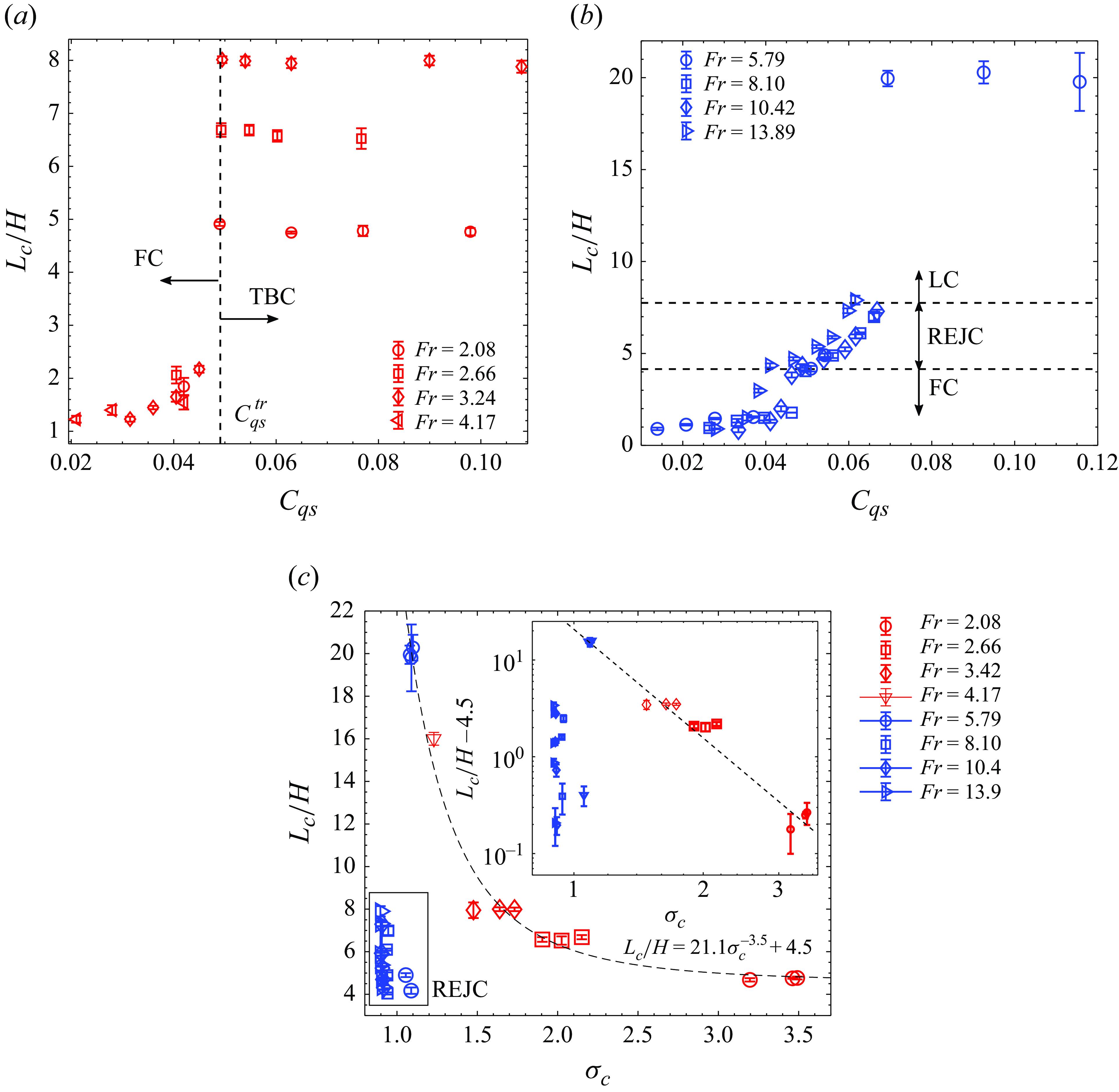
Figure 10. The length ( $L_{c}$
) of ventilated cavities, normalised by wedge height (
$L_{c}$
) of ventilated cavities, normalised by wedge height ( $H$
) at different
$H$
) at different $\textit{Fr}$
as a function of ventilation coefficient (
$\textit{Fr}$
as a function of ventilation coefficient ( $C_{qs}$
): (a) cavities at low
$C_{qs}$
): (a) cavities at low $\textit{Fr}$
(
$\textit{Fr}$
( $\lt$
5), (b) cavities at higher
$\lt$
5), (b) cavities at higher $\textit{Fr}$
(
$\textit{Fr}$
( $\gt$
5). (c) Supercavity length variation with cavitation number (
$\gt$
5). (c) Supercavity length variation with cavitation number ( $\sigma _{c}$
) (the low-
$\sigma _{c}$
) (the low- $\textit{Fr}$
cases are shown by red markers, while the high-
$\textit{Fr}$
cases are shown by red markers, while the high- $\textit{Fr}$
cases are shown by blue markers). The black dashed curve shows a power-law fit. The inset shows the same plot on an adjusted logarithmic scale.
$\textit{Fr}$
cases are shown by blue markers). The black dashed curve shows a power-law fit. The inset shows the same plot on an adjusted logarithmic scale.
3.5. Dynamics at cavity closure and gas ejection mechanisms
3.5.1. Foamy cavities
Foamy cavities do not have a well-defined closure, akin to natural open cavities defined by Laberteaux & Ceccio (Reference Laberteaux and Ceccio2001). These are wake-dominated cavities wherein the entrained gas is ejected out periodically via an alternating Von Kármán vortex street. This is shown by void fraction time-series in figure 11 (shown in supplementary movie 1 available at https://doi.org/10.1017/jfm.2025.10266). The gas ejection frequency, expressed as Strouhal number ( $St_{H}$
), is estimated to be
$St_{H}$
), is estimated to be ${\sim}0.31$
. This is higher than the Strouhal number 0.25 reported for a non-cavitating wedge of comparable blockage ratio and wedge-angle (Ramamurthy & Bhaskaran Reference Ramamurthy and Bhaskaran1978; Wu et al. Reference Wu, Deijlen, Bhatt, Ganesh and Ceccio2021). This increase in Strouhal number, also observed in natural cavitating wakes (Young & Holl Reference Young and Holl1966), can be attributed to vorticity dilatation due to the presence of cavitating structure (Belahadji et al. Reference Belahadji, Franc and Michel1995; Brandao et al. Reference Brandao, Bhatt and Mahesh2019) and mixture compressibility effects (Wu et al. Reference Wu, Deijlen, Bhatt, Ganesh and Ceccio2021).
${\sim}0.31$
. This is higher than the Strouhal number 0.25 reported for a non-cavitating wedge of comparable blockage ratio and wedge-angle (Ramamurthy & Bhaskaran Reference Ramamurthy and Bhaskaran1978; Wu et al. Reference Wu, Deijlen, Bhatt, Ganesh and Ceccio2021). This increase in Strouhal number, also observed in natural cavitating wakes (Young & Holl Reference Young and Holl1966), can be attributed to vorticity dilatation due to the presence of cavitating structure (Belahadji et al. Reference Belahadji, Franc and Michel1995; Brandao et al. Reference Brandao, Bhatt and Mahesh2019) and mixture compressibility effects (Wu et al. Reference Wu, Deijlen, Bhatt, Ganesh and Ceccio2021).
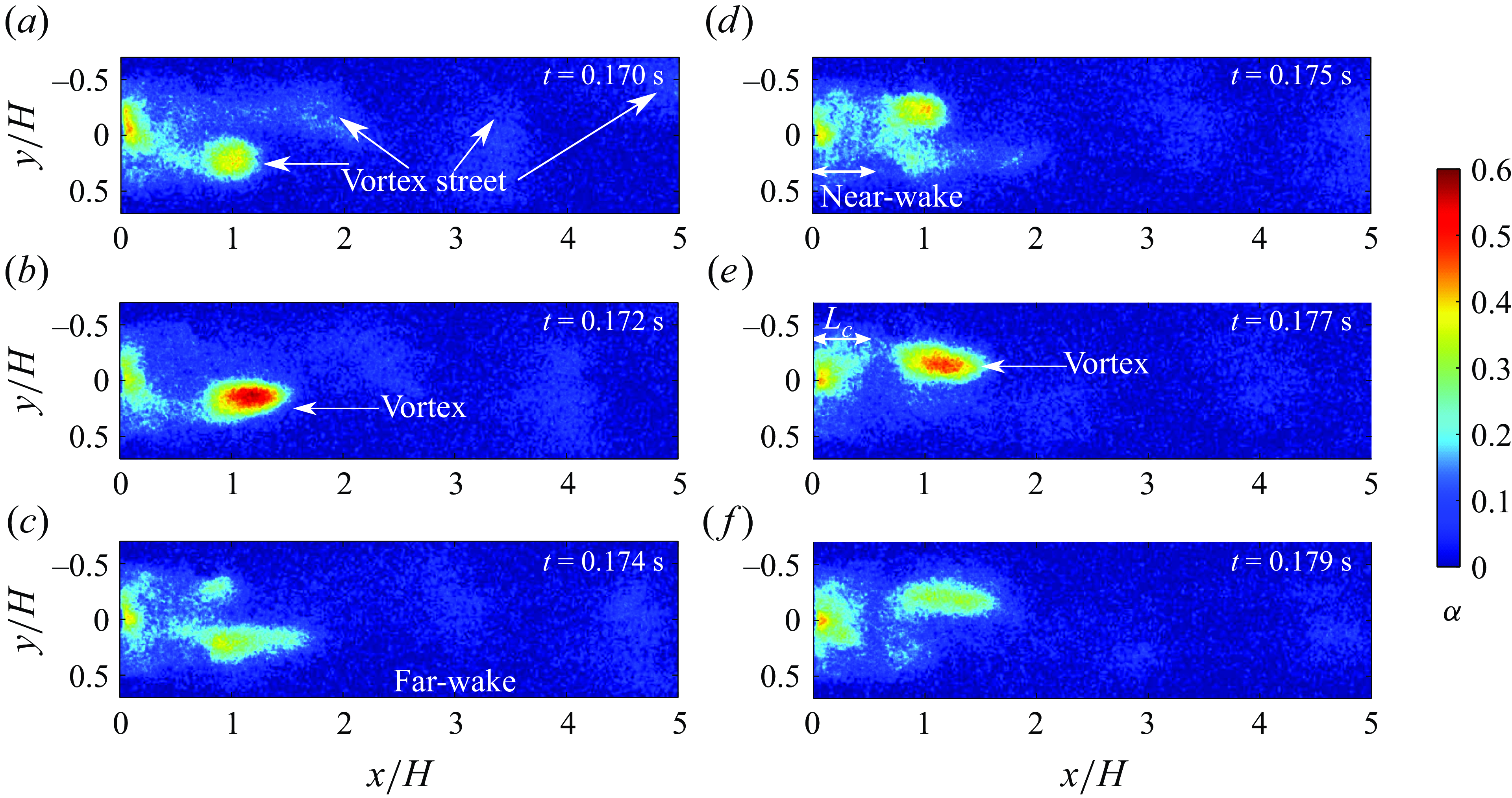
Figure 11. Instantaneous void fraction fields for an FC at $\textit{Fr}$
= 13.9,
$\textit{Fr}$
= 13.9, $C_{qs}$
= 0.0205, showing periodic gas ejection via a Von Kármán vortex street (time increases from (a) to (f)).
$C_{qs}$
= 0.0205, showing periodic gas ejection via a Von Kármán vortex street (time increases from (a) to (f)).
3.5.2. Twin-branched cavities
Twin-branched cavities are nominally two-dimensional until their bifurcation point but have a well-defined three-dimensional closure. The closure of these cavities is characterised by two branches along the walls as shown in figures 4 and 12. The cavity closure is marked by a weak re-entrant flow along the centreline of the cavity in the $x{-}z$
plane shown in figure 4(b).
$x{-}z$
plane shown in figure 4(b).
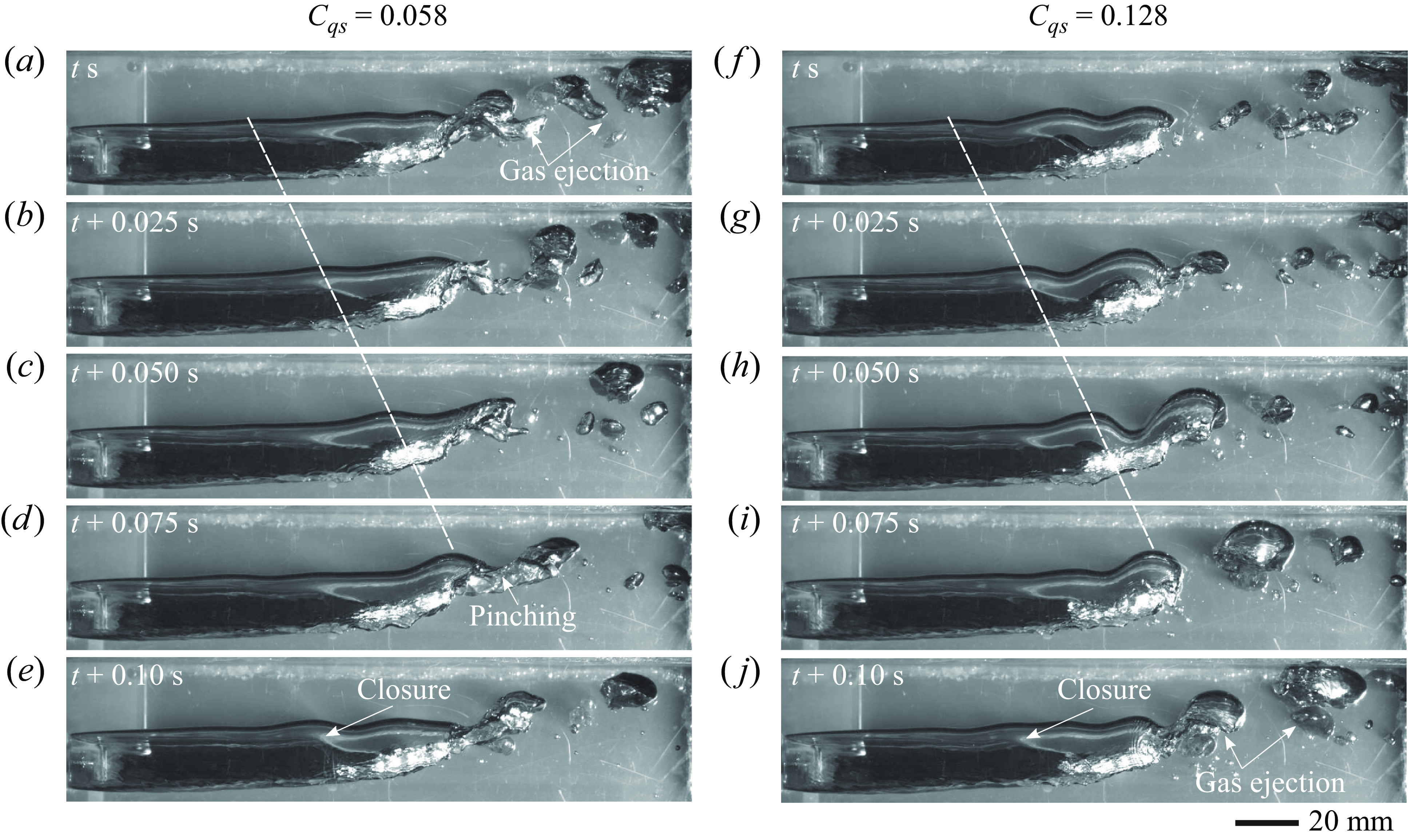
Figure 12. High-speed visualisation of TBC closure at $\textit{Fr}$
= 2.08 for two different cases of ventilation: (a–e)
$\textit{Fr}$
= 2.08 for two different cases of ventilation: (a–e) $C_{qs}$
= 0.058, (f–j)
$C_{qs}$
= 0.058, (f–j) $C_{qs}$
= 0.128. The white dashed line shows a convecting perturbation on the upper cavity interface responsible for cavity pinching.
$C_{qs}$
= 0.128. The white dashed line shows a convecting perturbation on the upper cavity interface responsible for cavity pinching.
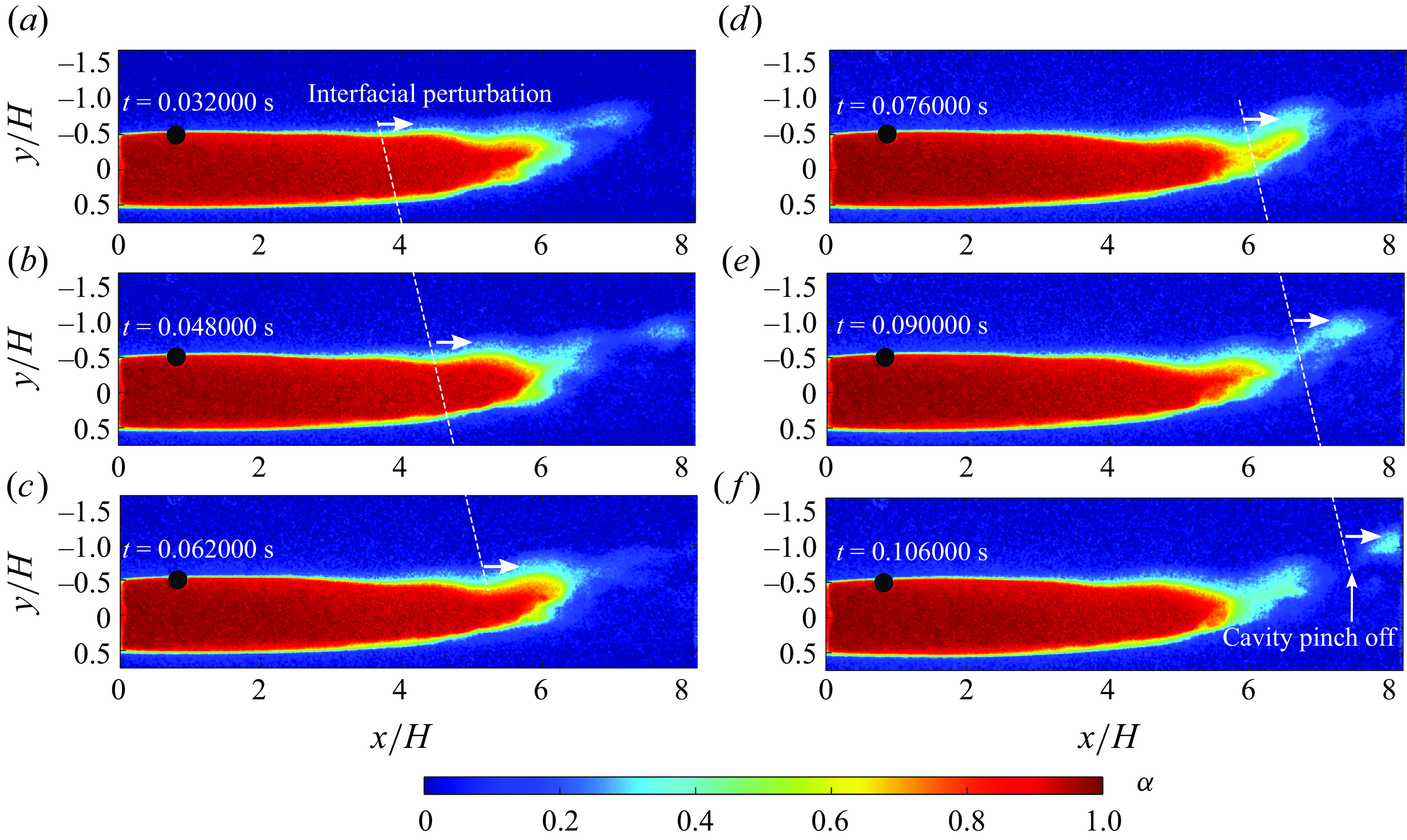
Figure 13. Instantaneous gas ejection in TBC closure at $\textit{Fr}$
= 2.08,
$\textit{Fr}$
= 2.08, $C_{qs}$
= 0.058. The white arrows show the travelling front of the interfacial perturbation eventually pinching the cavity-off. The white dashed line indicates the convection of a trough region of the perturbation.
$C_{qs}$
= 0.058. The white arrows show the travelling front of the interfacial perturbation eventually pinching the cavity-off. The white dashed line indicates the convection of a trough region of the perturbation.
Based on high-speed videos, two gas ejection mechanisms can be identified. Firstly, the gas ejection appears to be due to a re-entrant flow in the narrow midtail region, where gas is ejected intermittently in small parcels as shown in the region marked by ‘closure’ in figure 4(a,b). See supplementary movie 2 for the visualisation of cavity span ( $x{-}z$
plane). Secondly, gas ejection is observed at the downstream tips of the two branches via travelling disturbance on the interface and oscillations shown in figure 12 and supplementary movie 3. Figure 13(a–f) and supplementary movie 4 show X-ray-based visualisations of gas ejection from interface oscillation in TBCs. The white arrow shows the propagation of the disturbance along the interface.
$x{-}z$
plane). Secondly, gas ejection is observed at the downstream tips of the two branches via travelling disturbance on the interface and oscillations shown in figure 12 and supplementary movie 3. Figure 13(a–f) and supplementary movie 4 show X-ray-based visualisations of gas ejection from interface oscillation in TBCs. The white arrow shows the propagation of the disturbance along the interface.
As the travelling disturbance propagates downstream along the cavity interface shown in figure 13(a–e), it pinches the cavity at the twin branches in combination with in-plane oscillations leading to a gas ejection. Since the length of the cavity does not change with increasing $C_{qs}$
for a given
$C_{qs}$
for a given $\textit{Fr}$
(see figure 10
a), larger gas ejection must occur at higher
$\textit{Fr}$
(see figure 10
a), larger gas ejection must occur at higher $C_{qs}$
. The larger gas ejection at
$C_{qs}$
. The larger gas ejection at $C_{qs}=0.128$
appears as larger slugs as shown in figure 12(f–j). It is observed that the amplitude of the instability is higher for larger ventilation (
$C_{qs}=0.128$
appears as larger slugs as shown in figure 12(f–j). It is observed that the amplitude of the instability is higher for larger ventilation ( $C_{qs}$
) for a given
$C_{qs}$
) for a given $\textit{Fr}$
, suggesting a higher degree of pulsation at higher
$\textit{Fr}$
, suggesting a higher degree of pulsation at higher $C_{qs}$
. The convecting wavefront is marked by a white dashed line in figure 12 for
$C_{qs}$
. The convecting wavefront is marked by a white dashed line in figure 12 for $C_{qs}$
= 0.058 (a–e) and 0.128 (f–j). The slopes of the white dashed lines can be used to approximate the propagation speed of the perturbation and appear to be near identical, despite a significant difference in
$C_{qs}$
= 0.058 (a–e) and 0.128 (f–j). The slopes of the white dashed lines can be used to approximate the propagation speed of the perturbation and appear to be near identical, despite a significant difference in $C_{qs}$
. For a given
$C_{qs}$
. For a given $\textit{Fr}$
, the propagation velocity is close to the velocity of the upper cavity interface (
$\textit{Fr}$
, the propagation velocity is close to the velocity of the upper cavity interface ( $\mathcal{O}(U_{0})$
) for the considered range of
$\mathcal{O}(U_{0})$
) for the considered range of $C_{qs}$
(
$C_{qs}$
( $\approx$
0.058–0.128). We hypothesis that it is an inertial wave/disturbance possibly triggered by the combination of Kelvin–Helmholtz instability due to the shear at the cavity interface and Rayleigh–Taylor instability due to the density difference at the upper cavity interface (Jiang & Cheng Reference Jiang and Cheng2019). The propagation speed of instability (
$\approx$
0.058–0.128). We hypothesis that it is an inertial wave/disturbance possibly triggered by the combination of Kelvin–Helmholtz instability due to the shear at the cavity interface and Rayleigh–Taylor instability due to the density difference at the upper cavity interface (Jiang & Cheng Reference Jiang and Cheng2019). The propagation speed of instability ( $c_{r, tbc}$
) at the interface of two fluids in the absence of a bounding wall, estimated using linear stability analysis, is given by
$c_{r, tbc}$
) at the interface of two fluids in the absence of a bounding wall, estimated using linear stability analysis, is given by $c_{r, tbc} = (\rho _{g}U_{g} + \rho _{l}U_{l})/({\rho _{g}+ \rho _{l}}) \approx U_{l} \approx U_{0}$
(Drazin Reference Drazin2002), where subscripts
$c_{r, tbc} = (\rho _{g}U_{g} + \rho _{l}U_{l})/({\rho _{g}+ \rho _{l}}) \approx U_{l} \approx U_{0}$
(Drazin Reference Drazin2002), where subscripts $l$
,
$l$
, $g$
correspond to liquid and gas phases, respectively. For
$g$
correspond to liquid and gas phases, respectively. For $\rho _{g} \ll \rho _{l}$
,
$\rho _{g} \ll \rho _{l}$
, $c_{r, tbc}$
reduces to
$c_{r, tbc}$
reduces to $ U_{l}$
due to the large density difference across the cavity interface. This is consistent with our experimental observations, i.e. the propagation velocity of the perturbation is of the order of inflow velocity.
$ U_{l}$
due to the large density difference across the cavity interface. This is consistent with our experimental observations, i.e. the propagation velocity of the perturbation is of the order of inflow velocity.
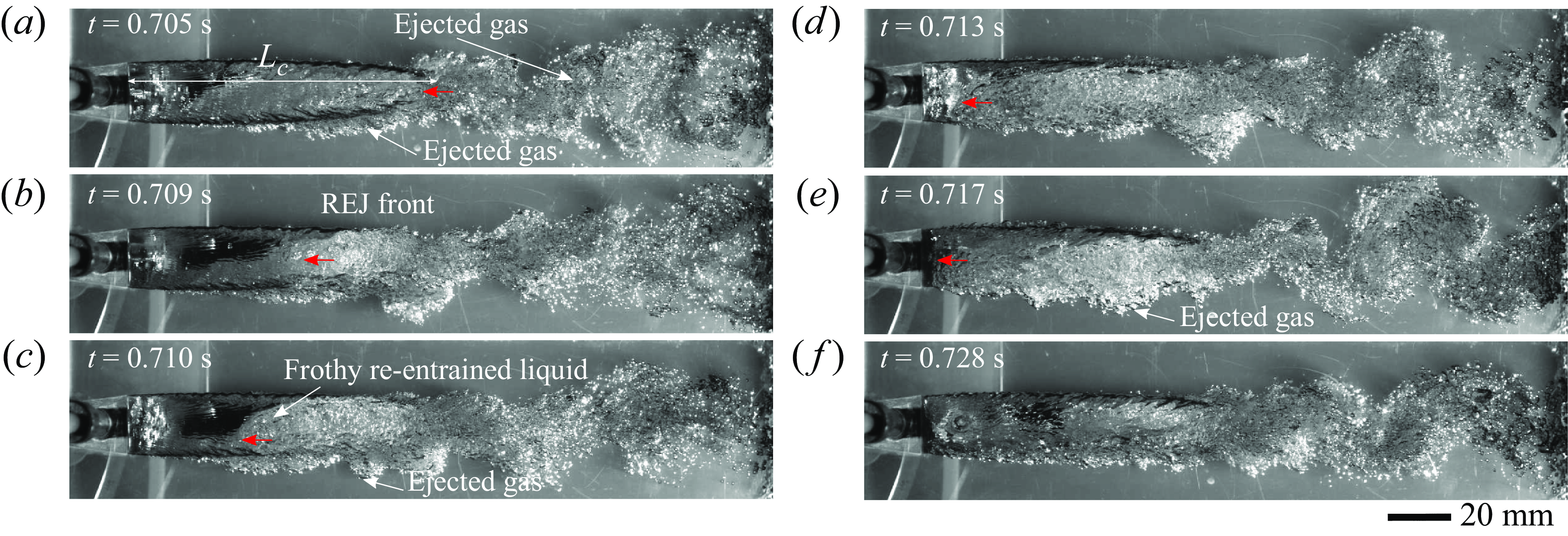
Figure 14. High-speed visualisation of REJC dynamics at $\textit{Fr} = 5.79$
,
$\textit{Fr} = 5.79$
, $C_{qs} = 0.054$
. The red arrows in (a–e) indicate the re-entrant flow. The Von Kármán vortex street can be clearly seen in the wake of the cavity.
$C_{qs} = 0.054$
. The red arrows in (a–e) indicate the re-entrant flow. The Von Kármán vortex street can be clearly seen in the wake of the cavity.
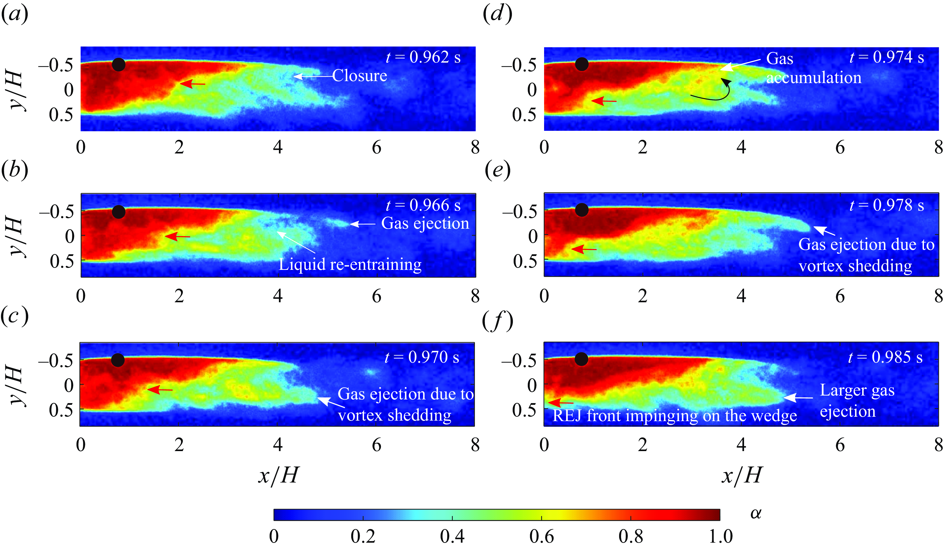
Figure 15. Instantaneous void fraction fields for an REJC at $\textit{Fr}$
= 5.79,
$\textit{Fr}$
= 5.79, $C_{qs}$
= 0.054 showing gas accumulation and ejection. Red arrows indicate the re-entrant flow front propagating upstream.
$C_{qs}$
= 0.054 showing gas accumulation and ejection. Red arrows indicate the re-entrant flow front propagating upstream.
3.5.3. Re-entrant jet cavities
A time-series obtained from high-speed videography of an REJC is shown in figure 14. A re-entrant flow, visualised by a frothy mixture along with the flow front indicated by a red arrow, can be seen propagating upstream in figure 14(a–e). As the re-entrant flow reaches the base of the wedge, it appears to be redirected to the cavity interfaces. This is illustrated in supplementary movie 5. A clearly defined Von Kármán vortex street can be seen in the cavity wake (see figure 14
d,e), suggesting (i) vortex shedding and gas ejection are coupled, (ii) strong wake–gas interaction in such cavities. As the re-entrant jet front propagates upstream, it displaces gas at the bottom of the cavity as seen in figure 14(c,e). While the gas can be seen advecting away from the cavity, the gas volume cannot be quantified from the high-speed imaging. Time-resolved void fraction measurements of an REJC for the same condition show the internal cavity flow structures in figure 15 and supplementary movie 6. Note that the X-ray densitometry measurements are separate experimental trials from the high-speed optical measurements. The gas accumulation in the upper half of the cavity is evident from the red regions (high void fraction, $\alpha \simeq 1$
) in figure 15. Supplementary movie 6 shows that a part of injected gas reaches near the closure and accumulates in the upper part of the cavity, as also indicated by figure 15(d). The other part of the injected gas is ejected from the lower half of the supercavity via a quasiperiodic vortex. This quasiperiodicity in lower vortex shedding is suspected to be induced by the presence of bubbly re-entrant flow in the lower portion of the supercavity. The accumulated gas in the upper portion of the cavity is ejected out at the top interface in the form of a periodic vortex. The gas ejection via the spanwise vortices in the form of the wake is shown in figure 15(b–e). The re-entrant flow is visualised by a low-void-fraction (
$\alpha \simeq 1$
) in figure 15. Supplementary movie 6 shows that a part of injected gas reaches near the closure and accumulates in the upper part of the cavity, as also indicated by figure 15(d). The other part of the injected gas is ejected from the lower half of the supercavity via a quasiperiodic vortex. This quasiperiodicity in lower vortex shedding is suspected to be induced by the presence of bubbly re-entrant flow in the lower portion of the supercavity. The accumulated gas in the upper portion of the cavity is ejected out at the top interface in the form of a periodic vortex. The gas ejection via the spanwise vortices in the form of the wake is shown in figure 15(b–e). The re-entrant flow is visualised by a low-void-fraction ( $\sim$
0.5) region in the lower part of the cavity. The re-entrant jet is formed near the closure, propagates towards the wedge base and becomes confined to the bottom part of the cavity due to the effects of gravity (see figure 15). Here the red arrows indicate the re-entrant flow front. Figure 15(f) shows that the propagating re-entrant flow displaces the gas, resulting in an additional gas ejection. This re-entrant flow cycle continues to sustain a nearly fixed-length REJC. The detailed analyses of the re-entrant jet dynamics showing bimodal gas ejection is included in Appendix A.
$\sim$
0.5) region in the lower part of the cavity. The re-entrant jet is formed near the closure, propagates towards the wedge base and becomes confined to the bottom part of the cavity due to the effects of gravity (see figure 15). Here the red arrows indicate the re-entrant flow front. Figure 15(f) shows that the propagating re-entrant flow displaces the gas, resulting in an additional gas ejection. This re-entrant flow cycle continues to sustain a nearly fixed-length REJC. The detailed analyses of the re-entrant jet dynamics showing bimodal gas ejection is included in Appendix A.
3.5.4. Long cavities
Closure of LCs could not be observed using high-speed images as it spanned beyond the FOV. Nevertheless, X-ray-based flow visualisation was performed through the thicker and denser PVC walls of the test facility at FOV-2, as shown in figure 1. This led to a low SNR in the void fraction, allowing only qualitative cavity visualisation. From these qualitative visualisations, the following observations were made: LCs do not exhibit a re-entrant flow-like closure. The gas appears to be ejected near the cavity closure via an interfacial perturbation and pulsations shown in figure 16(a) and supplementary movie 7. The perturbation is seen to be convecting on the cavity interface with a velocity close to inflow velocity ( $U_{0}$
). Such cavity pulsations have been observed by Michel (Reference Michel1984) in LCs at large
$U_{0}$
). Such cavity pulsations have been observed by Michel (Reference Michel1984) in LCs at large $C_{qs}$
. The gas pocket shed off at the closure shown by the
$C_{qs}$
. The gas pocket shed off at the closure shown by the $x{-}t$
diagram in figure 16(b) is periodic with a non-dimensional frequency (
$x{-}t$
diagram in figure 16(b) is periodic with a non-dimensional frequency ( $St_{H}$
) of approximately 0.19. This is in close agreement with Shao et al. (Reference Shao, Li, Yoon and Hong2022), who reported an average
$St_{H}$
) of approximately 0.19. This is in close agreement with Shao et al. (Reference Shao, Li, Yoon and Hong2022), who reported an average $St$
of 0.20 for oscillatory cavities in an axisymmetric cavitator. It is observed that with an even further increase in
$St$
of 0.20 for oscillatory cavities in an axisymmetric cavitator. It is observed that with an even further increase in $C_{qs}$
, the cavity lengths do not increase substantially, rather, the amplitude of oscillation increases. Future studies are planned to investigate LCs in detail.
$C_{qs}$
, the cavity lengths do not increase substantially, rather, the amplitude of oscillation increases. Future studies are planned to investigate LCs in detail.
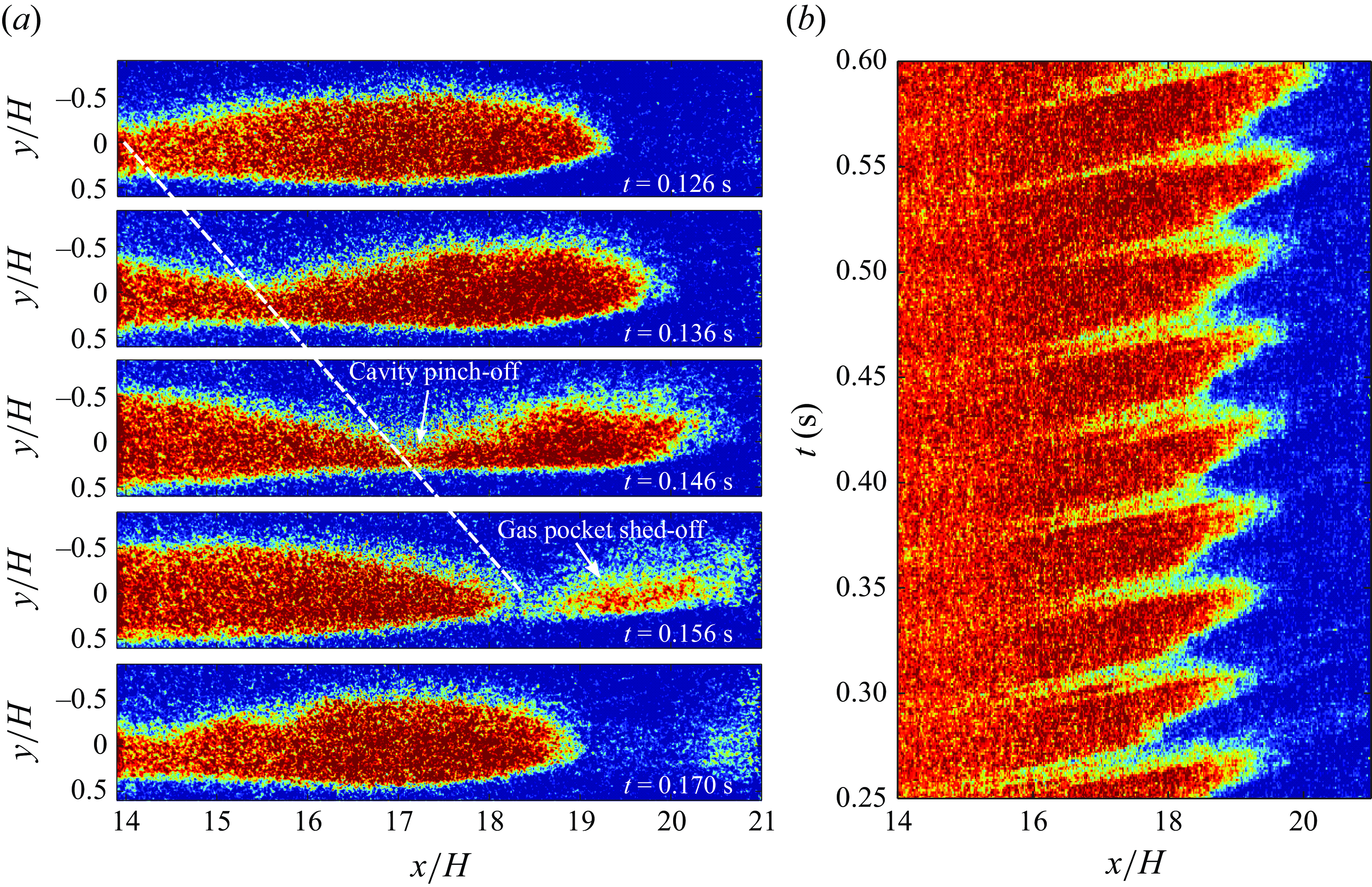
Figure 16. (a) X-ray visualisation of cavity closure corresponding to the LC regime at $\textit{Fr} = 5.79$
,
$\textit{Fr} = 5.79$
, $C_{qs} = 0.069$
. X-ray images were acquired through the thicker and denser PVC walls of the test section, leading to highly reduced SNR. As such, the void fraction cannot be accurately estimated. However, the shape of the cavity can be visualised well. The white dashed line shows the travelling perturbation front leading to the gas pocket shed off at the closure. (b) The
$C_{qs} = 0.069$
. X-ray images were acquired through the thicker and denser PVC walls of the test section, leading to highly reduced SNR. As such, the void fraction cannot be accurately estimated. However, the shape of the cavity can be visualised well. The white dashed line shows the travelling perturbation front leading to the gas pocket shed off at the closure. (b) The $x{-}t$
diagram at
$x{-}t$
diagram at $y/H \approx 0$
for LC closure showing nine gas shedding cycles.
$y/H \approx 0$
for LC closure showing nine gas shedding cycles.
3.6. Compressibility effects
In natural cavitating flows, the compressibility of the medium plays a significant role in dictating cavity dynamics (Ganesh et al. Reference Ganesh, Mäkiharju and Ceccio2016; Wu et al. Reference Wu, Deijlen, Bhatt, Ganesh and Ceccio2021). Moderately high vapour fractions ( $\sim$
0.4–0.7) in combination with low pressure in the vapour cavity (of the order of vapour pressure) reduces the speed of sound in this bubbly mixture to
$\sim$
0.4–0.7) in combination with low pressure in the vapour cavity (of the order of vapour pressure) reduces the speed of sound in this bubbly mixture to $\mathcal{O}(1)$
ms
$\mathcal{O}(1)$
ms $^{-1}$
. This can result in high cavity Mach numbers, giving rise to the propagating bubbly/condensation shock fronts as observed experimentally by Ganesh et al. (Reference Ganesh, Mäkiharju and Ceccio2016), Gawandalkar & Poelma (Reference Gawandalkar and Poelma2024) and numerically by Budich, Schmidt & Adams (Reference Budich, Schmidt and Adams2018). In ventilated cavities, the void fraction can attain values close to 0.5 leading to lower speed of sound, and hence a high Mach number. Hence, the effects of compressibility bear significant industrial implications and need to be examined for ventilated cavities. The direct void fraction (
$^{-1}$
. This can result in high cavity Mach numbers, giving rise to the propagating bubbly/condensation shock fronts as observed experimentally by Ganesh et al. (Reference Ganesh, Mäkiharju and Ceccio2016), Gawandalkar & Poelma (Reference Gawandalkar and Poelma2024) and numerically by Budich, Schmidt & Adams (Reference Budich, Schmidt and Adams2018). In ventilated cavities, the void fraction can attain values close to 0.5 leading to lower speed of sound, and hence a high Mach number. Hence, the effects of compressibility bear significant industrial implications and need to be examined for ventilated cavities. The direct void fraction ( $\alpha$
) and pressure measurements (
$\alpha$
) and pressure measurements ( $P_{c}$
) allow us to estimate the speed of sound in the binary mixture within the cavity (
$P_{c}$
) allow us to estimate the speed of sound in the binary mixture within the cavity ( $c_{m}$
), using (3.1) (Brennen Reference Brennen1995), where
$c_{m}$
), using (3.1) (Brennen Reference Brennen1995), where $k$
is the polytropic constant of the mixture. In (3.1) it is assumed that the cavity is composed of liquid (subscript
$k$
is the polytropic constant of the mixture. In (3.1) it is assumed that the cavity is composed of liquid (subscript $l$
) and gas (subscript
$l$
) and gas (subscript $g$
) with negligible surface tension effects, bubble dynamics, and mass transfer between phases. The Mach number,
$g$
) with negligible surface tension effects, bubble dynamics, and mass transfer between phases. The Mach number, $Ma$
, is then estimated with (3.2), where the velocity scale
$Ma$
, is then estimated with (3.2), where the velocity scale $u$
is either the inflow velocity (
$u$
is either the inflow velocity ( $U_{0}$
) or the velocity of the re-entrant jet front (
$U_{0}$
) or the velocity of the re-entrant jet front ( $\overline {u_{rej}}$
):
$\overline {u_{rej}}$
):
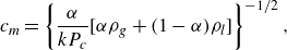 \begin{align}& c_{m} = \left \{ \frac {\alpha _{}}{kP_{c}} [\alpha _{} \rho _{g} + (1-\alpha _{}) \rho _{l} ]\right \} ^ {-{1}/{2}}, \end{align}
 \begin{align}&\qquad\qquad\quad Ma = \frac {u}{c_{m}}. \end{align}
The TBC and LC are filled with air ( $\alpha \sim 1$
) as seen by the void fraction distribution shown in figure 9(b,d). Hence, the speed of sound is expected to be high in these cavities, resulting in low Mach numbers at
$\alpha \sim 1$
) as seen by the void fraction distribution shown in figure 9(b,d). Hence, the speed of sound is expected to be high in these cavities, resulting in low Mach numbers at $u$
. These cavities are omitted from the analyses. Further, using
$u$
. These cavities are omitted from the analyses. Further, using $U_{0}$
as a velocity scale to estimate
$U_{0}$
as a velocity scale to estimate $Ma$
provides us with the maximum achievable values of
$Ma$
provides us with the maximum achievable values of $Ma$
for the cavity. The time-averaged void fraction fields are used to estimate the local
$Ma$
for the cavity. The time-averaged void fraction fields are used to estimate the local $Ma$
for FCs and REJCs in figure 17(a,b). It is seen that the Mach number is consistently lower than 0.3. The estimated Mach number of re-entrant flow front (
$Ma$
for FCs and REJCs in figure 17(a,b). It is seen that the Mach number is consistently lower than 0.3. The estimated Mach number of re-entrant flow front ( $Ma_{rej}$
, based on
$Ma_{rej}$
, based on $\overline {u}_{rej}$
) is shown in figure 17(c). It increases with
$\overline {u}_{rej}$
) is shown in figure 17(c). It increases with $\textit{Fr}$
, yet remains lower than 0.1. This suggests that the effect of compressibility is negligible for the ventilated cavities under consideration. Although the void fractions are sufficiently low, the pressure in the cavities is sufficiently high to maintain the speed of sound as high as 25 ms
$\textit{Fr}$
, yet remains lower than 0.1. This suggests that the effect of compressibility is negligible for the ventilated cavities under consideration. Although the void fractions are sufficiently low, the pressure in the cavities is sufficiently high to maintain the speed of sound as high as 25 ms $^{-1}$
. This is in contrast with natural cavities, where the speed of sound (
$^{-1}$
. This is in contrast with natural cavities, where the speed of sound ( $c_{m}$
) drops to a few ms
$c_{m}$
) drops to a few ms $^{-1}$
owing to low cavity pressures close to vapour pressures of a few kPa demonstrated by Gawandalkar & Poelma (Reference Gawandalkar and Poelma2024). Hence, the bubbly shock fronts observed in natural cavitation flow are not observed in ventilated cavities under consideration.
$^{-1}$
owing to low cavity pressures close to vapour pressures of a few kPa demonstrated by Gawandalkar & Poelma (Reference Gawandalkar and Poelma2024). Hence, the bubbly shock fronts observed in natural cavitation flow are not observed in ventilated cavities under consideration.
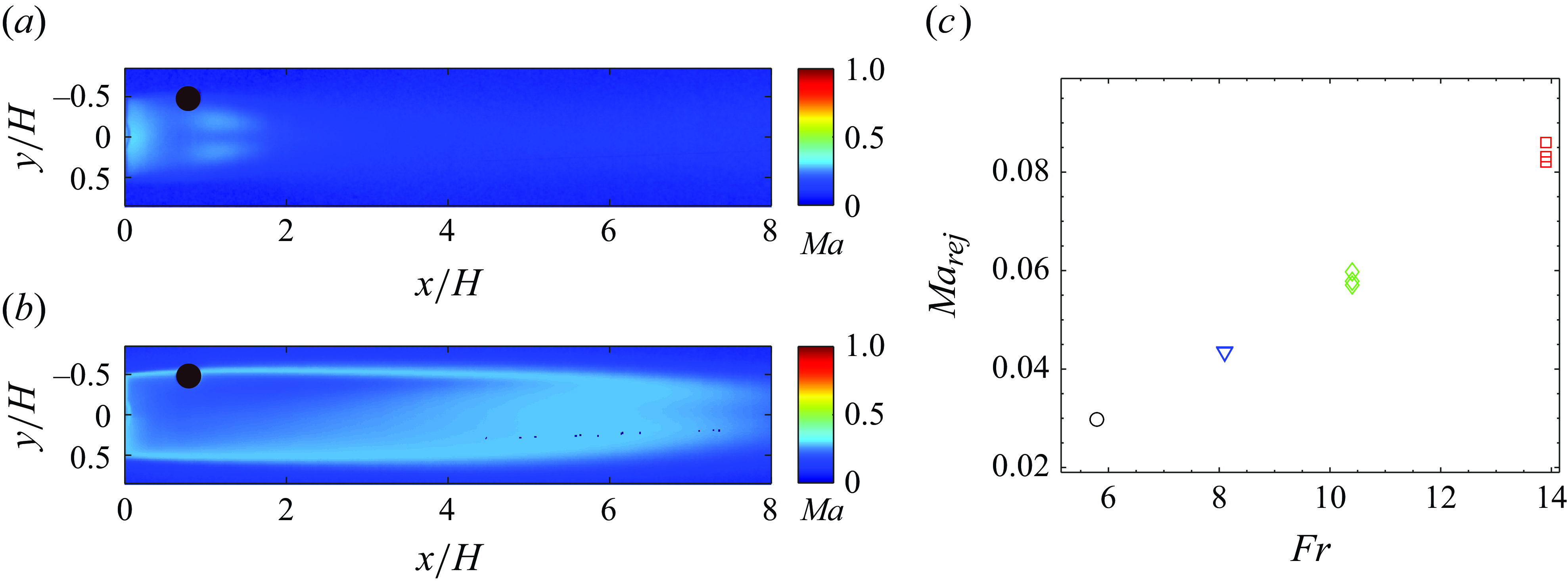
Figure 17. Mach number ( $Ma$
) based on averaged void fraction fields (
$Ma$
) based on averaged void fraction fields ( $\overline {\alpha }$
) and incoming velocity (
$\overline {\alpha }$
) and incoming velocity ( $U_{0}$
) at (a)
$U_{0}$
) at (a) $\textit{Fr}=13.89$
,
$\textit{Fr}=13.89$
, $C_{qs}= 0.029$
, (b)
$C_{qs}= 0.029$
, (b) $\textit{Fr}=13.89$
,
$\textit{Fr}=13.89$
, $C_{qs}= 0.0617$
. (c) Mach number of the re-entrant jet front at different
$C_{qs}= 0.0617$
. (c) Mach number of the re-entrant jet front at different $\textit{Fr}$
and
$\textit{Fr}$
and $C_{qs}$
.
$C_{qs}$
.
4. Formation of supercavities
During the formation of supercavities, cavity length undergoes an abrupt increase at $C^{tr}_{qs} \sim C_{qs}^{tr} (C_{qs, fc-tbc}^{tr}, C_{qs, fc-rejc}^{tr}, C_{qs, rejc-lc}^{tr})$
as shown by the regime map in figure 7 and cavity length variation in figure 10(a,b). This abrupt increase in length is also accompanied by a change in cavity closure type. Such cavities observed during the formation process are referred to as transitional cavities, and the corresponding closures as transitional closures. Transitional cavity closures dictate the ventilation demands and the stability of the fully formed supercavities. Hence, the formation of supercavities, with an emphasis on transitional closure region, is discussed in this section.
$C^{tr}_{qs} \sim C_{qs}^{tr} (C_{qs, fc-tbc}^{tr}, C_{qs, fc-rejc}^{tr}, C_{qs, rejc-lc}^{tr})$
as shown by the regime map in figure 7 and cavity length variation in figure 10(a,b). This abrupt increase in length is also accompanied by a change in cavity closure type. Such cavities observed during the formation process are referred to as transitional cavities, and the corresponding closures as transitional closures. Transitional cavity closures dictate the ventilation demands and the stability of the fully formed supercavities. Hence, the formation of supercavities, with an emphasis on transitional closure region, is discussed in this section.
The formation of supercavities (TBCs and LCs) was studied with an L-H ventilation strategy shown by a red $C_{qs}$
profile in figure 2. Using time-synchronous measurements of void fraction fields (
$C_{qs}$
profile in figure 2. Using time-synchronous measurements of void fraction fields ( $\alpha (x, y, t)$
) and the ventilation input (
$\alpha (x, y, t)$
) and the ventilation input ( $\dot {Q}_{in}(t)$
), change in cavity volume (
$\dot {Q}_{in}(t)$
), change in cavity volume ( $V_{g,c}(t)$
) was estimated to quantify gas leakage (
$V_{g,c}(t)$
) was estimated to quantify gas leakage ( $\dot {Q}_{out}(t)$
). In a control volume around the cavity, the mass balance of gas inside the cavity is given by (4.1), where
$\dot {Q}_{out}(t)$
). In a control volume around the cavity, the mass balance of gas inside the cavity is given by (4.1), where $\rho _{c}$
is the mass density,
$\rho _{c}$
is the mass density, $V_{c}$
is the cavity volume and
$V_{c}$
is the cavity volume and $\dot {Q}$
is the volumetric gas flux. The subscript
$\dot {Q}$
is the volumetric gas flux. The subscript $g$
denotes the gas phase, while
$g$
denotes the gas phase, while $in$
and
$in$
and $out$
denote gas injection and ejection, respectively:
$out$
denote gas injection and ejection, respectively:
 \begin{equation} \frac {\partial \rho _{g,c}V_{g,c}}{\partial {t}} = \rho _{g} \dot {Q}_{g,in} - \rho _{g} \dot {Q}_{g,out}. \end{equation}
Equaton (4.1) can be rearranged to estimate the ratio of ejected to injected gas from the cavity expressed as $\Theta _{f}$
, computed as per (4.2). The
$\Theta _{f}$
, computed as per (4.2). The $\Theta _{f}$
is directly proportional to the gas ejection rate out of the cavity and inversely proportional to the gas entrainment rate inside the cavity:
$\Theta _{f}$
is directly proportional to the gas ejection rate out of the cavity and inversely proportional to the gas entrainment rate inside the cavity:
 \begin{equation} \Theta _{f} = \frac {\dot {Q}_{g,out}}{\dot {Q}_{g,in}} (t) = 1 - \frac {1}{\dot {Q}_{g,in}(t)} \frac {\partial \alpha (x,y,t) V_{c}(t)}{t}. \end{equation}
In 4.2, $\dot {Q}_{g,in}(t)$
is the prescribed injection profile, and
$\dot {Q}_{g,in}(t)$
is the prescribed injection profile, and $V_{c}(t)=\iint _{{CV}}W {{\rm d}x} {{\rm d}y}$
is the estimated cavity volume from the X-ray-based void fraction fields. The control volume is a rectangle between
$V_{c}(t)=\iint _{{CV}}W {{\rm d}x} {{\rm d}y}$
is the estimated cavity volume from the X-ray-based void fraction fields. The control volume is a rectangle between $y/H=-0.65$
and
$y/H=-0.65$
and $0.65$
for the full extent of the X-ray FOV. Note that
$0.65$
for the full extent of the X-ray FOV. Note that $\Theta _{f}$
estimation is limited to snapshots where the entire cavity is within the X-ray FOV. The estimated instantaneous cavity volume (
$\Theta _{f}$
estimation is limited to snapshots where the entire cavity is within the X-ray FOV. The estimated instantaneous cavity volume ( $V_{c}(t)$
) is smoothed using a cubic smoothing spline with
$V_{c}(t)$
) is smoothed using a cubic smoothing spline with $p=0.99$
(De Boor Reference De Boor1978). Quasistable cavities are expected to satisfy
$p=0.99$
(De Boor Reference De Boor1978). Quasistable cavities are expected to satisfy $\Theta _{f}\approx 1$
, i.e. gas injection is in equilibrium with gas ejection. The formation of TBCs at
$\Theta _{f}\approx 1$
, i.e. gas injection is in equilibrium with gas ejection. The formation of TBCs at $\textit{Fr} \approx$
2.08, 4.17 and LCs at
$\textit{Fr} \approx$
2.08, 4.17 and LCs at $\textit{Fr} \approx 10.42$
are discussed separately in §§ 4.1 and 4.2, respectively.
$\textit{Fr} \approx 10.42$
are discussed separately in §§ 4.1 and 4.2, respectively.
4.1. Formation of TBCs
Figure 18. (a–h) X-ray densitometry snapshots of TBC formation at $\textit{Fr}= 2.08$
and final
$\textit{Fr}= 2.08$
and final $C_{qs} = 0.075$
. (i) The temporal variation of the ventilation coefficient,
$C_{qs} = 0.075$
. (i) The temporal variation of the ventilation coefficient, $C_{qs}$
(solid line), and instantaneous ejection ratio,
$C_{qs}$
(solid line), and instantaneous ejection ratio, $\Theta _{f}$
(dotted line). The grey region indicates the transitional closure region.
$\Theta _{f}$
(dotted line). The grey region indicates the transitional closure region.
Figure 18 shows the formation of a TBC based on time-resolved X-ray measurements at $\textit{Fr} = 2.08$
,
$\textit{Fr} = 2.08$
, $C_{qs}=0.075$
. Initially, small bubbles accumulate near the top of the wedge as shown in figure 18(a,b). The gas ejection ratio,
$C_{qs}=0.075$
. Initially, small bubbles accumulate near the top of the wedge as shown in figure 18(a,b). The gas ejection ratio, $\Theta _{f}$
, decreases with increasing
$\Theta _{f}$
, decreases with increasing $C_{qs}$
and the cavity begins to expand towards the bottom of the wedge, as shown in figure 18(b–d). The decrease in
$C_{qs}$
and the cavity begins to expand towards the bottom of the wedge, as shown in figure 18(b–d). The decrease in $\Theta _{f}$
can be attributed to the formation of transitional closure leading to the increased gas entrainment to form a supercavity. As the cavity height increases to reach near-wedge height (
$\Theta _{f}$
can be attributed to the formation of transitional closure leading to the increased gas entrainment to form a supercavity. As the cavity height increases to reach near-wedge height ( $H$
), it rapidly increases in length due to the formed closure with no observable re-entrant flow (figure 18
c–e). This coincides with
$H$
), it rapidly increases in length due to the formed closure with no observable re-entrant flow (figure 18
c–e). This coincides with $\Theta _{f}$
attaining a near-constant value of 0.2 as shown in the grey region in figure 18(i). It is important to note that the cavity is nominally two-dimensional during the growth or transition phase. During cavity growth,
$\Theta _{f}$
attaining a near-constant value of 0.2 as shown in the grey region in figure 18(i). It is important to note that the cavity is nominally two-dimensional during the growth or transition phase. During cavity growth, $\Theta _{f}$
exhibits slight oscillatory behaviour due to the gas ejection, via cavity pinching at the closure. Figure 18(e–g) shows the formation of cavity branches along the wall, a characteristic of TBCs discussed earlier. Although oscillatory,
$\Theta _{f}$
exhibits slight oscillatory behaviour due to the gas ejection, via cavity pinching at the closure. Figure 18(e–g) shows the formation of cavity branches along the wall, a characteristic of TBCs discussed earlier. Although oscillatory, $\Theta _{f}$
increases in figures 18(e) to 18(g) from 0.2 to 1. This suggests that the cavity is approaching a fully developed state, i.e.
$\Theta _{f}$
increases in figures 18(e) to 18(g) from 0.2 to 1. This suggests that the cavity is approaching a fully developed state, i.e. $\dot {Q}_{g,in}$
is in equilibrium with
$\dot {Q}_{g,in}$
is in equilibrium with $ \dot {Q}_{g,out}$
. The cavity at such low
$ \dot {Q}_{g,out}$
. The cavity at such low $\textit{Fr}$
exhibits a significant degree of camber and the closure is marked by an interfacial perturbation responsible for gas ejection. The cavity formation dynamics is shown in supplementary movie 8.
$\textit{Fr}$
exhibits a significant degree of camber and the closure is marked by an interfacial perturbation responsible for gas ejection. The cavity formation dynamics is shown in supplementary movie 8.
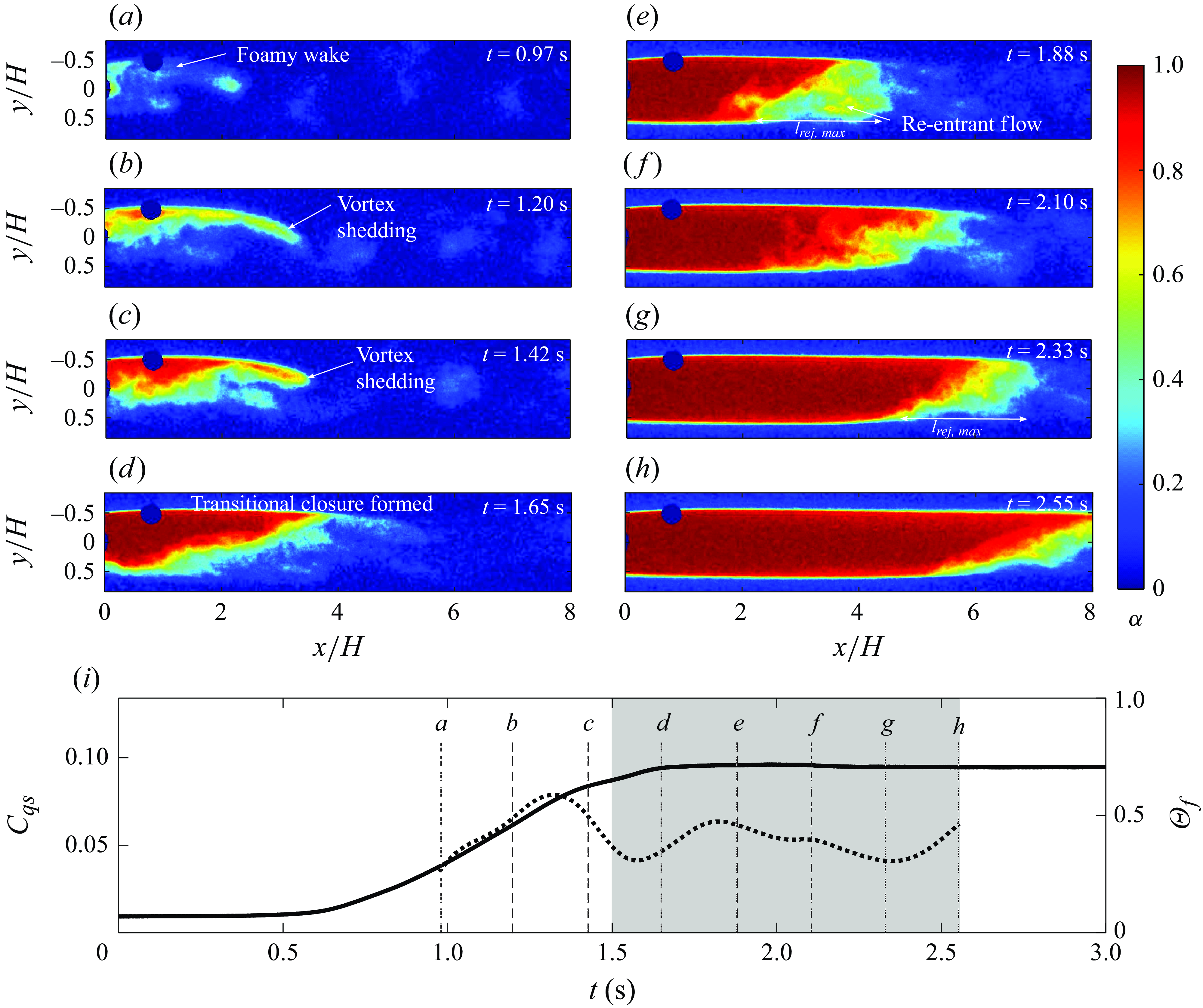
Figure 19. (a)–(h) X-ray densitometry snapshots of TBC formation at $\textit{Fr}= 4.17$
and
$\textit{Fr}= 4.17$
and $C_{qs} = 0.096$
. (i) The time-dependent ventilation coefficient,
$C_{qs} = 0.096$
. (i) The time-dependent ventilation coefficient, $C_{qs}$
(solid line), and instantaneous ejection ratio,
$C_{qs}$
(solid line), and instantaneous ejection ratio, $\Theta _{f}$
(dotted line).
$\Theta _{f}$
(dotted line).
Figure 19 shows the formation of a TBC at $\textit{Fr} = 4.2$
and
$\textit{Fr} = 4.2$
and $C_{qs}=0.096$
. The formation dynamics is different due to the increased effect of flow inertia. Initially, there is a dispersed, foamy wake behind the wedge, and gas ejection due to the vortex shedding is seen in figure 19(a–c), similar to figure 18(a,b). With an increase in injection rate (
$C_{qs}=0.096$
. The formation dynamics is different due to the increased effect of flow inertia. Initially, there is a dispersed, foamy wake behind the wedge, and gas ejection due to the vortex shedding is seen in figure 19(a–c), similar to figure 18(a,b). With an increase in injection rate ( $Q_{g,in}$
),
$Q_{g,in}$
), $\Theta _{f}$
, although oscillatory, decreases to approximately 0.4 near point d in figure 19(i), suggesting increased gas entrainment. The observed oscillation in
$\Theta _{f}$
, although oscillatory, decreases to approximately 0.4 near point d in figure 19(i), suggesting increased gas entrainment. The observed oscillation in $\Theta _{f}$
is attributed to gas ejection by spanwise vortex streets, as shown in figure 19(b,c). The aforementioned features are visualised in supplementary movie 9. The decrease in
$\Theta _{f}$
is attributed to gas ejection by spanwise vortex streets, as shown in figure 19(b,c). The aforementioned features are visualised in supplementary movie 9. The decrease in $\Theta _{f}$
in figure 19(d–h) coincides with the formation of transitional closure and relatively rapid gas accumulation near the top of the wedge, increasing the cavity length. Interestingly, during the cavity growth (after the formation of transitional closure),
$\Theta _{f}$
in figure 19(d–h) coincides with the formation of transitional closure and relatively rapid gas accumulation near the top of the wedge, increasing the cavity length. Interestingly, during the cavity growth (after the formation of transitional closure), $\Theta _{f}$
remains almost constant at approximately 0.4, shown by the grey region in figure 19(i). This behaviour is similar to the previous case of
$\Theta _{f}$
remains almost constant at approximately 0.4, shown by the grey region in figure 19(i). This behaviour is similar to the previous case of $\textit{Fr}$
= 2.08, where
$\textit{Fr}$
= 2.08, where $\Theta _{f}$
maintained a near-constant value 0.2. As the cavity grows, the upper cavity interface curves downwards as evident in figure 19(d). This downward curvature near the cavity closure is in contrast to the upward curvature seen at the lower-
$\Theta _{f}$
maintained a near-constant value 0.2. As the cavity grows, the upper cavity interface curves downwards as evident in figure 19(d). This downward curvature near the cavity closure is in contrast to the upward curvature seen at the lower- $\textit{Fr}$
case shown in figure 18. The downward curvature is accompanied by a fixed-length re-entrant flow (
$\textit{Fr}$
case shown in figure 18. The downward curvature is accompanied by a fixed-length re-entrant flow ( $l_{rej,max}$
) at the cavity closure as visualised in figure 19(e–h) by the low void fraction region (
$l_{rej,max}$
) at the cavity closure as visualised in figure 19(e–h) by the low void fraction region ( $\alpha \approx$
0.5) in the lower half of the cavity. As the cavity grows in length, the re-entrant flow front recedes further away from the wedge base as shown in figure 19(d–h). The transitional cavities are nominally two-dimensional in contrast to fully formed TBCs with three-dimensional closure. Furthermore, the structure of the transitional closure is seen to be dependent on the flow inertia (
$\alpha \approx$
0.5) in the lower half of the cavity. As the cavity grows in length, the re-entrant flow front recedes further away from the wedge base as shown in figure 19(d–h). The transitional cavities are nominally two-dimensional in contrast to fully formed TBCs with three-dimensional closure. Furthermore, the structure of the transitional closure is seen to be dependent on the flow inertia ( $\textit{Fr}$
,
$\textit{Fr}$
, $Re_{H}$
), addressed in § 4.3.
$Re_{H}$
), addressed in § 4.3.
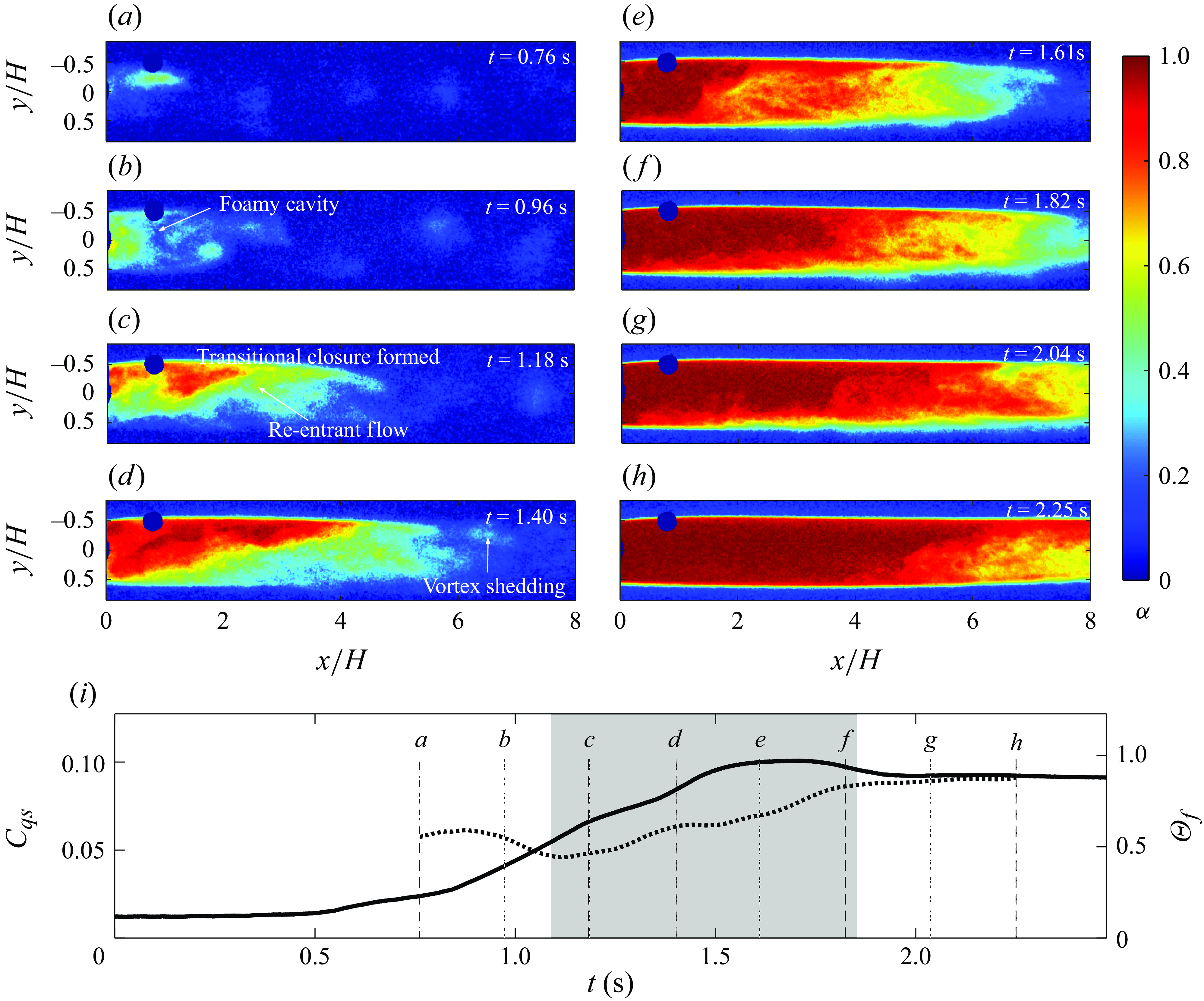
Figure 20. (a–h) X-ray densitometry snapshots of LC formation at $\textit{Fr}= 10.4$
and
$\textit{Fr}= 10.4$
and $C_{qs} = 0.090$
. (i) Temporal variation of the ventilation coefficient,
$C_{qs} = 0.090$
. (i) Temporal variation of the ventilation coefficient, $C_{qs}$
(solid line), and instantaneous ejection ratio,
$C_{qs}$
(solid line), and instantaneous ejection ratio, $\Theta _{f}$
(dotted line). The grey region indicates the transitional closure region.
$\Theta _{f}$
(dotted line). The grey region indicates the transitional closure region.
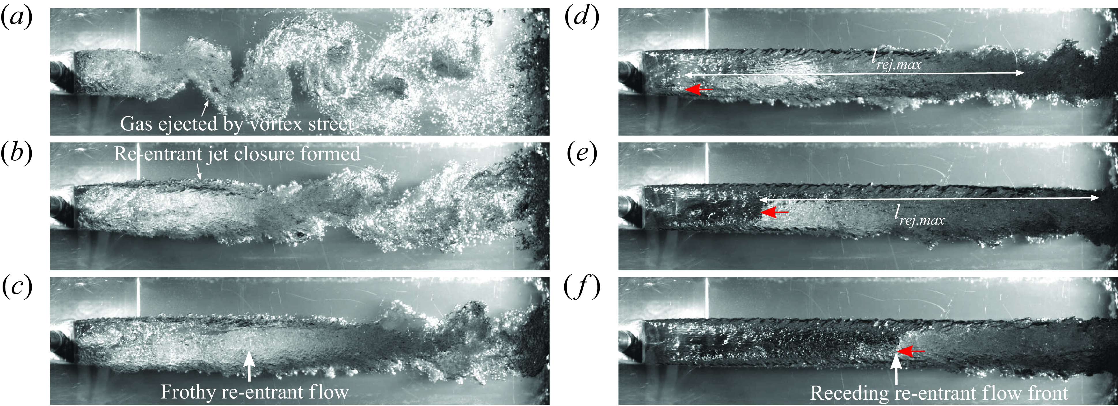
Figure 21. High-speed visualisation of LC formation (gas entrainment, liquid re-entrainment and gas ejection) at $\textit{Fr}$
= 10.4,
$\textit{Fr}$
= 10.4, $C_{qs}$
= 0.090. The red arrow indicates the re-entrant flow front as the cavity length increases.
$C_{qs}$
= 0.090. The red arrow indicates the re-entrant flow front as the cavity length increases.
4.2. Formation of LCs
Figure 20 shows the formation of LCs at $\textit{Fr}= 10.4$
and
$\textit{Fr}= 10.4$
and $C_{qs} = 0.090$
. The corresponding high-speed visualisations having a larger FOV shown in figure 21 facilitate a complete observation of flow structures at the closure region. As gas injection begins, an FC is formed, as shown in figure 20(a,b). As
$C_{qs} = 0.090$
. The corresponding high-speed visualisations having a larger FOV shown in figure 21 facilitate a complete observation of flow structures at the closure region. As gas injection begins, an FC is formed, as shown in figure 20(a,b). As $C_{qs}$
is increased, transitional closure is formed and supercavity formation begins near point cin figure 20(i). Thus FCs transitions to REJCs upon the formation of transitional closure with a re-entrant flow at point c. The value of
$C_{qs}$
is increased, transitional closure is formed and supercavity formation begins near point cin figure 20(i). Thus FCs transitions to REJCs upon the formation of transitional closure with a re-entrant flow at point c. The value of $\Theta _{f}$
reaches a minimum of 0.45, suggesting increased entrainment of injected gas in the wake, leading to an increase in cavity length as shown in figure 20(i). This results in a supercavity with a re-entrant flow spanning the entire cavity length (i.e. more than
$\Theta _{f}$
reaches a minimum of 0.45, suggesting increased entrainment of injected gas in the wake, leading to an increase in cavity length as shown in figure 20(i). This results in a supercavity with a re-entrant flow spanning the entire cavity length (i.e. more than $4H$
) and impinging on the wedge base at point din figure 20(i). The gas is ejected via re-entering liquid flow and spanwise vortices visualised by Von Kármán vortex streets in figure 21(b,c). Figure 20(e–h) shows that with a further increase in
$4H$
) and impinging on the wedge base at point din figure 20(i). The gas is ejected via re-entering liquid flow and spanwise vortices visualised by Von Kármán vortex streets in figure 21(b,c). Figure 20(e–h) shows that with a further increase in $C_{qs}$
, the re-entrant flow has assumed its maximum length similar to the
$C_{qs}$
, the re-entrant flow has assumed its maximum length similar to the $\textit{Fr} \approx 4.17$
case. As the REJC begins to transition to the LC, the re-entrant flow front can no longer impinge on the wedge base. Instead, it recedes away from the wedge base as the cavity length increases, as also reported by Barbaca et al. (Reference Barbaca, Pearce and Brandner2017). The transition of REJC to LC is shown by supplementary movie 10, and in figure 21(d–f), where the receding re-entrant flow front is indicated by a red arrow. During the transition, the length of the re-entrant flow remains constant (
$\textit{Fr} \approx 4.17$
case. As the REJC begins to transition to the LC, the re-entrant flow front can no longer impinge on the wedge base. Instead, it recedes away from the wedge base as the cavity length increases, as also reported by Barbaca et al. (Reference Barbaca, Pearce and Brandner2017). The transition of REJC to LC is shown by supplementary movie 10, and in figure 21(d–f), where the receding re-entrant flow front is indicated by a red arrow. During the transition, the length of the re-entrant flow remains constant ( $l_{rej, max}/H \approx 8.5$
) as its front recedes further away from the wedge base with the increase in cavity length. Interestingly, as the cavity length increases (after the formation of closure at point cin figure 20(i),
$l_{rej, max}/H \approx 8.5$
) as its front recedes further away from the wedge base with the increase in cavity length. Interestingly, as the cavity length increases (after the formation of closure at point cin figure 20(i), $\Theta _{f}$
does not maintain a constant value, rather it increases from 0.45 to 0.85 (see the grey region in figure 20
i), suggesting larger gas ejection rates in comparison with previous cases of low
$\Theta _{f}$
does not maintain a constant value, rather it increases from 0.45 to 0.85 (see the grey region in figure 20
i), suggesting larger gas ejection rates in comparison with previous cases of low $\textit{Fr}$
.
$\textit{Fr}$
.
The different trends in $\Theta _{f}$
with
$\Theta _{f}$
with $\textit{Fr}$
can be explained by the distinct closure types transitional cavities attain during the formation of TBCs and LCs: during the formation of a TBC, the transitional cavity has interfacial perturbations propagating towards the closure region or a mild re-entrant flow with vortex shedding, resulting in a smaller gas ejection rate. However, during the formation of an LC, the closure has a prominent re-entrant flow entering the cavity, resulting in a larger gas ejection. A prominent re-entrant flow at the closure seems to contribute to a significantly larger gas ejection than the interfacial perturbation or vortex shedding. This larger gas ejection rate likely leads to reduced gas entrainment, and hence stunted length of REJCs in figure 10(c). This is in line with the DIH measurements of Shao et al. (Reference Shao, Li, Yoon and Hong2022), who reported a large instantaneous gas ejection rate for cavities with re-entrant jet closure. This is further corroborated by the higher collapse rate of established supercavities at higher
$\textit{Fr}$
can be explained by the distinct closure types transitional cavities attain during the formation of TBCs and LCs: during the formation of a TBC, the transitional cavity has interfacial perturbations propagating towards the closure region or a mild re-entrant flow with vortex shedding, resulting in a smaller gas ejection rate. However, during the formation of an LC, the closure has a prominent re-entrant flow entering the cavity, resulting in a larger gas ejection. A prominent re-entrant flow at the closure seems to contribute to a significantly larger gas ejection than the interfacial perturbation or vortex shedding. This larger gas ejection rate likely leads to reduced gas entrainment, and hence stunted length of REJCs in figure 10(c). This is in line with the DIH measurements of Shao et al. (Reference Shao, Li, Yoon and Hong2022), who reported a large instantaneous gas ejection rate for cavities with re-entrant jet closure. This is further corroborated by the higher collapse rate of established supercavities at higher $\textit{Fr}$
cases having a prominent re-entrant flow at the closure (not shown here). The dynamics of re-entrant flow at the cavity closure with increasing
$\textit{Fr}$
cases having a prominent re-entrant flow at the closure (not shown here). The dynamics of re-entrant flow at the cavity closure with increasing $\textit{Fr}$
is discussed in the next subsection.
$\textit{Fr}$
is discussed in the next subsection.
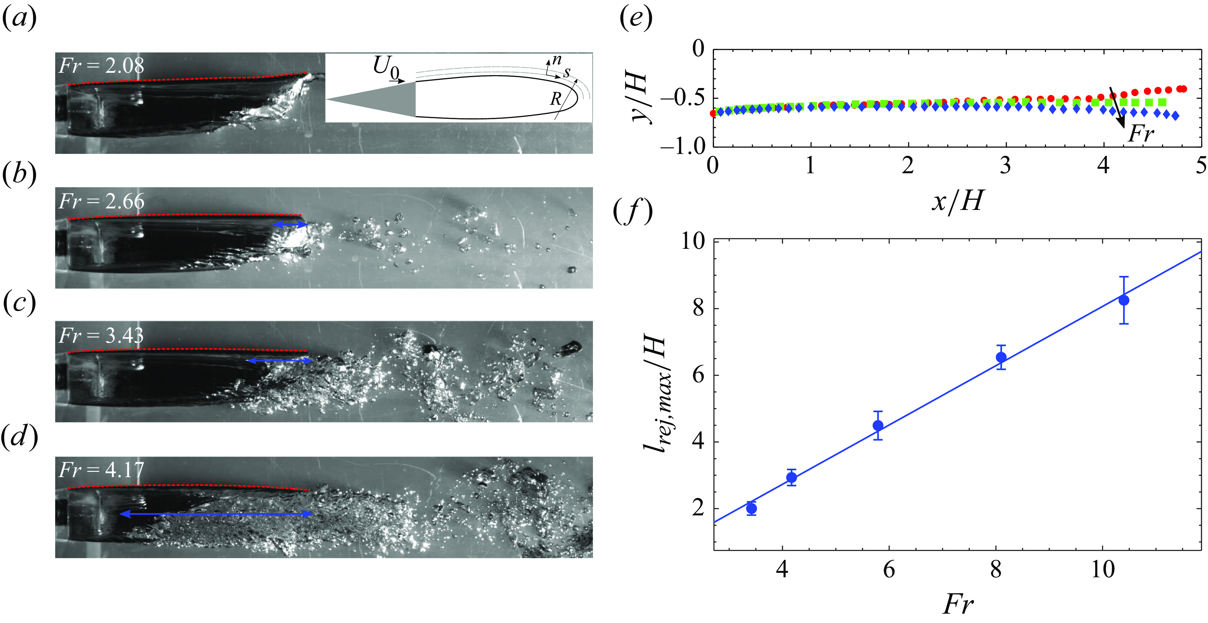
Figure 22. (a–d) Transitional cavity closure at a fixed cavity length seen at low- $\textit{Fr}$
range during the transition from FC to TBC. The blue markings show the length of the re-entrant flow, while the red dashed lines show the upper cavity interface. (e) The upper cavity interface as a function of
$\textit{Fr}$
range during the transition from FC to TBC. The blue markings show the length of the re-entrant flow, while the red dashed lines show the upper cavity interface. (e) The upper cavity interface as a function of $\textit{Fr}$
shows that the cavity interface curves downwards with an increase in
$\textit{Fr}$
shows that the cavity interface curves downwards with an increase in $\textit{Fr}$
. (f) The maximum re-entrant flow length (
$\textit{Fr}$
. (f) The maximum re-entrant flow length ( $l_{rej, max}/H$
) as a function of
$l_{rej, max}/H$
) as a function of $\textit{Fr}$
. The solid blue line is a linear fit:
$\textit{Fr}$
. The solid blue line is a linear fit: $0.85Fr-0.73$
.
$0.85Fr-0.73$
.
4.3. Effect of flow inertia on REJC closure
During the supercavity formation process, the length of the re-entrant flow attains a maximum, constant value, denoted by $l_{rej, max}$
(see blue arrows in figure 22
b–d). After
$l_{rej, max}$
(see blue arrows in figure 22
b–d). After $l_{rej, max}$
is attained, the re-entrant flow front cannot reach the wedge base, i.e.
$l_{rej, max}$
is attained, the re-entrant flow front cannot reach the wedge base, i.e. $l_{rej, max}$
is shorter than the cavity length. The existence of constant length re-entrant flow at the cavity closure during the supercavity formation is observed for
$l_{rej, max}$
is shorter than the cavity length. The existence of constant length re-entrant flow at the cavity closure during the supercavity formation is observed for $\textit{Fr} \geqslant$
3.43. It can be used as a proxy for the intensity of the re-entrant flow driven by a pressure gradient (Barbaca et al. Reference Barbaca, Pearce and Brandner2017). The
$\textit{Fr} \geqslant$
3.43. It can be used as a proxy for the intensity of the re-entrant flow driven by a pressure gradient (Barbaca et al. Reference Barbaca, Pearce and Brandner2017). The $l_{rej, max}$
is plotted for a range of
$l_{rej, max}$
is plotted for a range of $\textit{Fr}$
for a fixed cavity length in figure 22(f). It is seen to scale linearly with
$\textit{Fr}$
for a fixed cavity length in figure 22(f). It is seen to scale linearly with $\textit{Fr}$
:
$\textit{Fr}$
: $l_{rej, max}/H \sim 0.85 Fr - 0.73$
, suggesting that the re-entrant flow is getting stronger with flow inertia. Furthermore,
$l_{rej, max}/H \sim 0.85 Fr - 0.73$
, suggesting that the re-entrant flow is getting stronger with flow inertia. Furthermore, $l_{rej, max}$
is seen to be independent of the ventilation coefficient,
$l_{rej, max}$
is seen to be independent of the ventilation coefficient, $C_{qs}$
, for a given
$C_{qs}$
, for a given $\textit{Fr}$
(not shown here). This is in agreement with Barbaca et al. (Reference Barbaca, Pearce and Brandner2017, Reference Barbaca, Pearce, Ganesh, Ceccio and Brandner2019) who showed a similar behaviour of re-entrant jet length in natural and ventilated cavity flows behind a fence. It is worth noting that the increase in
$\textit{Fr}$
(not shown here). This is in agreement with Barbaca et al. (Reference Barbaca, Pearce and Brandner2017, Reference Barbaca, Pearce, Ganesh, Ceccio and Brandner2019) who showed a similar behaviour of re-entrant jet length in natural and ventilated cavity flows behind a fence. It is worth noting that the increase in $\textit{Fr}$
is accompanied by a stronger curvature of the upper cavity interface, resulting in a smaller radius of curvature
$\textit{Fr}$
is accompanied by a stronger curvature of the upper cavity interface, resulting in a smaller radius of curvature $R$
(see figure 22
e and inset in figure 22
a). For instance,
$R$
(see figure 22
e and inset in figure 22
a). For instance, $\textit{Fr}=2.08$
shows a slight upward curvature, while as
$\textit{Fr}=2.08$
shows a slight upward curvature, while as $\textit{Fr}$
increases, stronger downward curvature is exhibited by the upper cavity interface as shown in figure 22(e). This results in a smaller radius of curvature leading to a stronger adverse pressure gradient at the cavity closure as demonstrated by the 1-D Euler’s equation in streamline coordinate systems (4.3). Here,
$\textit{Fr}$
increases, stronger downward curvature is exhibited by the upper cavity interface as shown in figure 22(e). This results in a smaller radius of curvature leading to a stronger adverse pressure gradient at the cavity closure as demonstrated by the 1-D Euler’s equation in streamline coordinate systems (4.3). Here, $n$
is a direction normal to the radius of curvature in a streamline coordinate system, and
$n$
is a direction normal to the radius of curvature in a streamline coordinate system, and $R$
is the radius of curvature of the cavity closure (see inset in figure 22
a). A strong pressure gradient at the closure drives upstream, re-entrant flow from the closure region as also observed in natural cavitating flows (Callenaere et al. Reference Callenaere, Franc, Michel and Riondet2001; Gawandalkar & Poelma Reference Gawandalkar and Poelma2022):
$R$
is the radius of curvature of the cavity closure (see inset in figure 22
a). A strong pressure gradient at the closure drives upstream, re-entrant flow from the closure region as also observed in natural cavitating flows (Callenaere et al. Reference Callenaere, Franc, Michel and Riondet2001; Gawandalkar & Poelma Reference Gawandalkar and Poelma2022):
 \begin{equation} \frac {\partial p }{\partial n} \sim \rho \frac {U_{0}^{2}}{R}. \end{equation}
Furthermore, $l_{rej, max}/H$
possibly dictates the gas ejection out of the cavity when REJCs transition to LCs. Consequently, if the ventilation input can overcome the gas ejection due to the re-entering flow, the REJC transitions to an LC. This is verified quantitatively using a simple gas ejection model based on empirical relations obtained in this study as detailed in Appendix B. It is also recognised that above the critical Froude number of 5.7, the Reynolds number (
$l_{rej, max}/H$
possibly dictates the gas ejection out of the cavity when REJCs transition to LCs. Consequently, if the ventilation input can overcome the gas ejection due to the re-entering flow, the REJC transitions to an LC. This is verified quantitatively using a simple gas ejection model based on empirical relations obtained in this study as detailed in Appendix B. It is also recognised that above the critical Froude number of 5.7, the Reynolds number ( $Re_{H}$
) of the flow is a more suitable parameter than
$Re_{H}$
) of the flow is a more suitable parameter than $\textit{Fr}$
. However, the effect of
$\textit{Fr}$
. However, the effect of $Re_{H}$
and
$Re_{H}$
and $\textit{Fr}$
are coupled in this study and will be segregated in future experiments with different wedge geometries.
$\textit{Fr}$
are coupled in this study and will be segregated in future experiments with different wedge geometries.
5. Ventilation hysteresis
Differences between ventilated cavities established using the H-L ventilation strategy and the L-H ventilation strategy discussed so far are presented in this section.
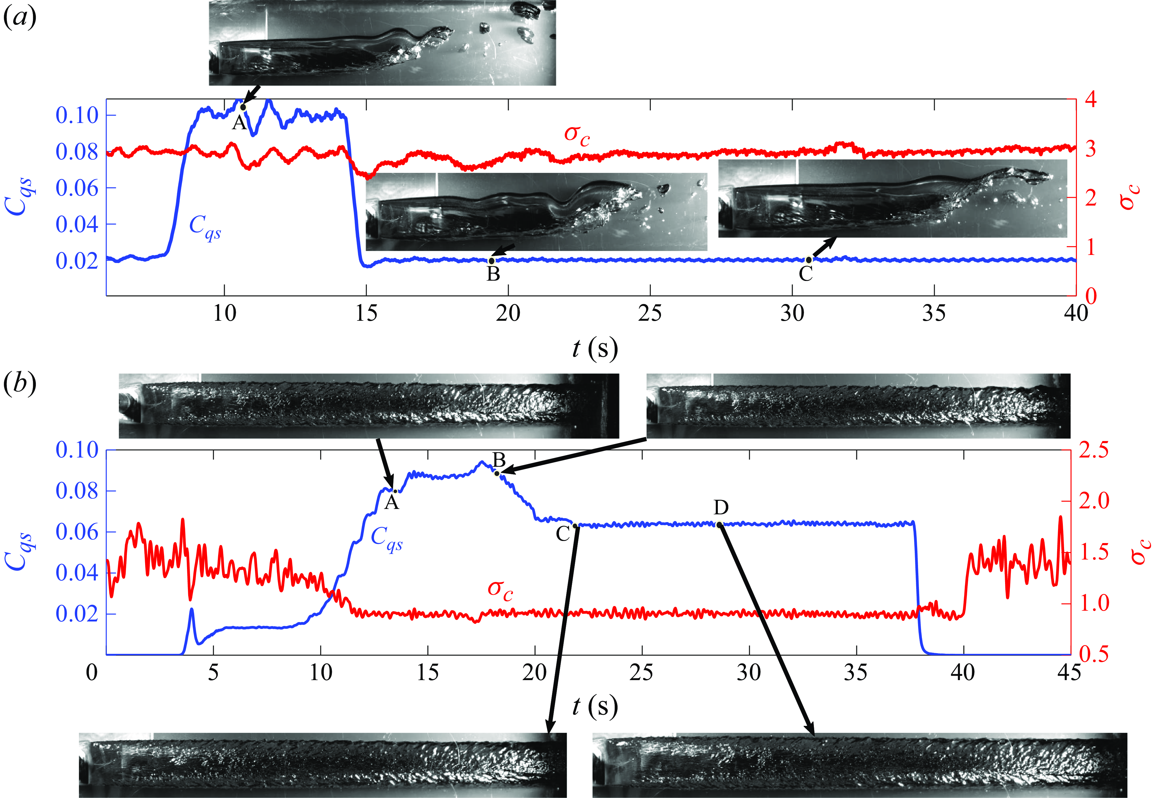
Figure 23. Time signals of $C_{qs}$
and
$C_{qs}$
and $\sigma _{c}$
showing ventilation hysteresis using H-L ventilation strategy for (a)
$\sigma _{c}$
showing ventilation hysteresis using H-L ventilation strategy for (a) $\textit{Fr}$
= 2.08: TBC is formed at A and can be maintained upon
$\textit{Fr}$
= 2.08: TBC is formed at A and can be maintained upon $C_{qs}$
reduction at B and C. (b)
$C_{qs}$
reduction at B and C. (b) $\textit{Fr}$
= 10.41: LC is formed at A and B, and can still be maintained upon
$\textit{Fr}$
= 10.41: LC is formed at A and B, and can still be maintained upon $C_{qs}$
reduction at C and D. The corresponding high–speed optical visualisations of the supercavity are shown.
$C_{qs}$
reduction at C and D. The corresponding high–speed optical visualisations of the supercavity are shown.
5.1. Supercavities formation with H-L ventilation strategy
Figures 23(a) and (b) show a representative case of supercavities formed with H-L ventilation strategy for TBC and LC, respectively. The temporal variation of $C_{qs}$
is shown in blue, and the cavity pressure variation expressed as
$C_{qs}$
is shown in blue, and the cavity pressure variation expressed as $\sigma _{c}$
is shown in red. In all cases considered, it is ensured that the cavity closure is fully developed, i.e. TBC at
$\sigma _{c}$
is shown in red. In all cases considered, it is ensured that the cavity closure is fully developed, i.e. TBC at $\textit{Fr} \approx$
2.08 and LC at
$\textit{Fr} \approx$
2.08 and LC at $\textit{Fr} \approx$
10.4, before reducing the ventilation coefficient to a prescribed
$\textit{Fr} \approx$
10.4, before reducing the ventilation coefficient to a prescribed $C_{qs}$
value.
$C_{qs}$
value.
At $\textit{Fr} \approx 2.08$
, the
$\textit{Fr} \approx 2.08$
, the $C_{qs}$
is initially set to 0.1 to ensure that the TBC is completely formed, as shown by point A in figure 23(a). Points B and C represent the region of reduced
$C_{qs}$
is initially set to 0.1 to ensure that the TBC is completely formed, as shown by point A in figure 23(a). Points B and C represent the region of reduced $C_{qs} \approx$
0.019. Interestingly, it is observed that the TBC persists at a much lower
$C_{qs} \approx$
0.019. Interestingly, it is observed that the TBC persists at a much lower $C_{qs}$
with the H-L strategy compared with the L-H strategy . At such a flow condition (
$C_{qs}$
with the H-L strategy compared with the L-H strategy . At such a flow condition ( $\textit{Fr}$
= 2.08,
$\textit{Fr}$
= 2.08, $C_{qs}$
= 0.019), FCs were observed in the L-H ventilation strategy as shown in figure 7.
$C_{qs}$
= 0.019), FCs were observed in the L-H ventilation strategy as shown in figure 7.
At a higher $\textit{Fr}$
(
$\textit{Fr}$
( $\approx$
10.4),
$\approx$
10.4), $C_{qs}$
is initially increased to 0.088 such that an LC is formed as shown by points A and B in figure 23(b). The reduction of
$C_{qs}$
is initially increased to 0.088 such that an LC is formed as shown by points A and B in figure 23(b). The reduction of $C_{qs}$
to 0.062 resulted in the persistence of the LC as shown by points C and D in figure 23(b). At the same flow conditions, REJCs were observed using the L-H strategy in the regime map of figure 7. It is observed that upon formation of a supercavity (TBC and LC), the cavitation number (
$C_{qs}$
to 0.062 resulted in the persistence of the LC as shown by points C and D in figure 23(b). At the same flow conditions, REJCs were observed using the L-H strategy in the regime map of figure 7. It is observed that upon formation of a supercavity (TBC and LC), the cavitation number ( $\sigma _{c}$
) remains relatively unchanged, with the reduction of the ventilation coefficient (
$\sigma _{c}$
) remains relatively unchanged, with the reduction of the ventilation coefficient ( $C_{qs}$
), as shown by the red line in figure 23. This corroborates our earlier observation that upon the formation of closure,
$C_{qs}$
), as shown by the red line in figure 23. This corroborates our earlier observation that upon the formation of closure, $\sigma _{c}$
does not vary with increasing
$\sigma _{c}$
does not vary with increasing $C_{qs}$
for fixed-length cavities (see figure 8
a). It is also consistent with the previous observations of Arndt et al. (Reference Arndt, Hambleton, Kawakami and Amromin2009) and Karn et al. (Reference Karn, Arndt and Hong2016) in other cavitator geometries. It is worthwhile to note that the previous studies of Karn et al. (Reference Karn, Arndt and Hong2016) observed a change in cavity closure with the reduction in
$C_{qs}$
for fixed-length cavities (see figure 8
a). It is also consistent with the previous observations of Arndt et al. (Reference Arndt, Hambleton, Kawakami and Amromin2009) and Karn et al. (Reference Karn, Arndt and Hong2016) in other cavitator geometries. It is worthwhile to note that the previous studies of Karn et al. (Reference Karn, Arndt and Hong2016) observed a change in cavity closure with the reduction in $C_{qs}$
, with no effect on cavity length (
$C_{qs}$
, with no effect on cavity length ( $L_{c}$
) and cavitation number (
$L_{c}$
) and cavitation number ( $\sigma _{c}$
). In this study, a change in the closure is not observed for TBCs; however, the closure of LCs is out of the optical FOV and needs further investigation. Nevertheless, qualitative observation with X-ray imaging in FOV-2 hints that closure remains unchanged. Furthermore, we observe that in-plane cavity oscillations are ‘damped-down’ upon
$\sigma _{c}$
). In this study, a change in the closure is not observed for TBCs; however, the closure of LCs is out of the optical FOV and needs further investigation. Nevertheless, qualitative observation with X-ray imaging in FOV-2 hints that closure remains unchanged. Furthermore, we observe that in-plane cavity oscillations are ‘damped-down’ upon $C_{qs}$
reduction.
$C_{qs}$
reduction.
5.2. Regime map with H-L ventilation strategy
A systematic variation of $\textit{Fr}$
and
$\textit{Fr}$
and $C_{qs}$
using H-L ventilation strategy resulted in the second regime map shown in figure 24(a). This regime map differs significantly from that based on the L-H ventilation strategy shown in figure 7. At low
$C_{qs}$
using H-L ventilation strategy resulted in the second regime map shown in figure 24(a). This regime map differs significantly from that based on the L-H ventilation strategy shown in figure 7. At low $\textit{Fr}$
, it is seen that the transition boundary from FC to TBC, denoted by the interface between the green and red regions in figure 24(a), increases monotonically with
$\textit{Fr}$
, it is seen that the transition boundary from FC to TBC, denoted by the interface between the green and red regions in figure 24(a), increases monotonically with $\textit{Fr}$
as opposed to a constant
$\textit{Fr}$
as opposed to a constant $C_{qs}$
= 0.043 in the regime map based on the L-H strategy. At higher
$C_{qs}$
= 0.043 in the regime map based on the L-H strategy. At higher $\textit{Fr}$
, the transition boundary between FC to LC, denoted as the interface between the black and red regions in figure 24(a), is similar to the FC to REJC transition in the L-H regime map (blue dotted line in figure 7). With the H-L ventilation strategy, LCs persist at comparable
$\textit{Fr}$
, the transition boundary between FC to LC, denoted as the interface between the black and red regions in figure 24(a), is similar to the FC to REJC transition in the L-H regime map (blue dotted line in figure 7). With the H-L ventilation strategy, LCs persist at comparable $C_{qs}$
where REJCs were observed for the L-H ventilation strategy. Further, they transition directly to FCs upon
$C_{qs}$
where REJCs were observed for the L-H ventilation strategy. Further, they transition directly to FCs upon $C_{qs}$
reduction. Thus, for a given
$C_{qs}$
reduction. Thus, for a given $\textit{Fr}$
and
$\textit{Fr}$
and $C_{qs}$
, the cavity closure, pressure and geometry depend on the ventilation strategy, in fact, ventilation history. Most importantly, from the regime maps, it is clear that the ventilation required to maintain a supercavity (
$C_{qs}$
, the cavity closure, pressure and geometry depend on the ventilation strategy, in fact, ventilation history. Most importantly, from the regime maps, it is clear that the ventilation required to maintain a supercavity ( $C_{qs,m}$
) is significantly different than the ventilation required to form a cavity (
$C_{qs,m}$
) is significantly different than the ventilation required to form a cavity ( $C_{qs,f}$
) as demonstrated in figure 24(b).
$C_{qs,f}$
) as demonstrated in figure 24(b).
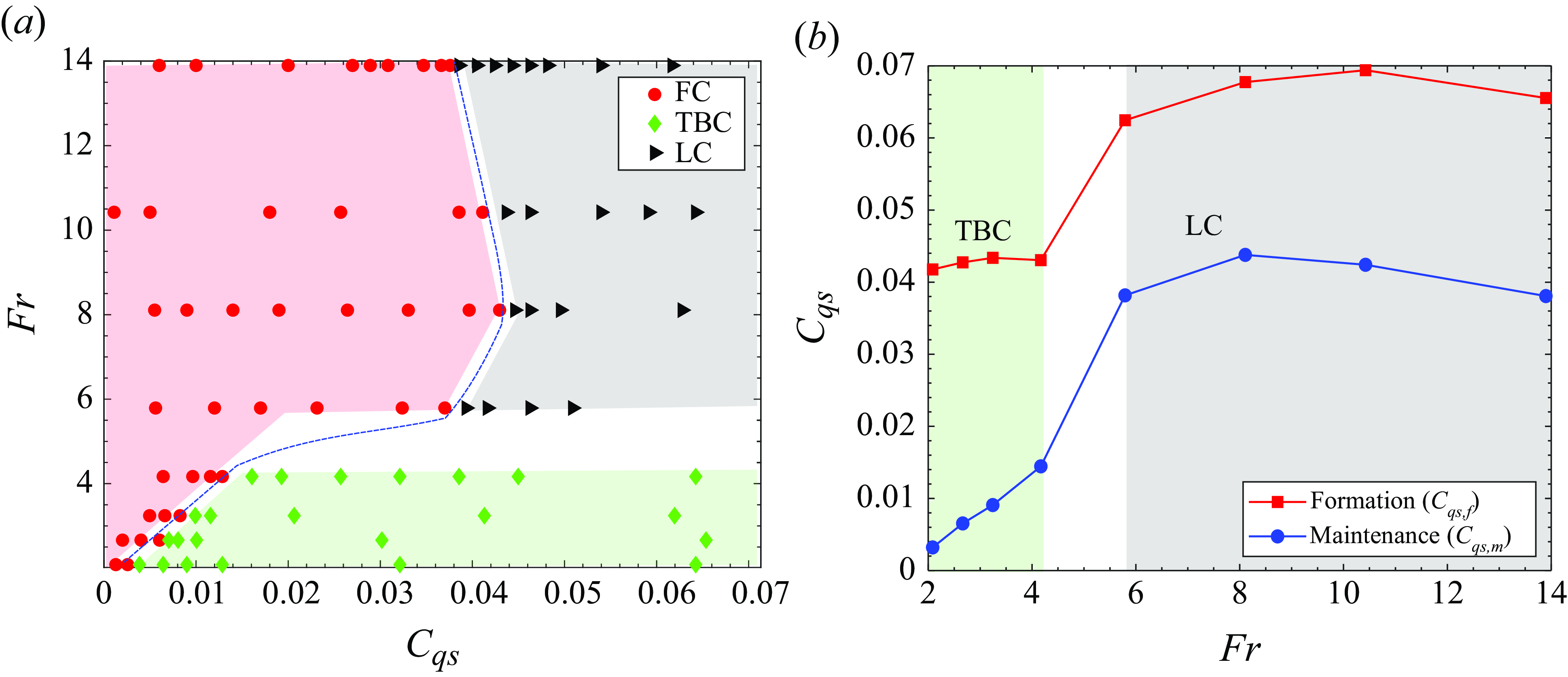
Figure 24. (a) Cavity regime map resulting from decreasing ventilation from a fully developed supercavity initial condition (H-L ventilation strategy). The blue dashed line shows the $C_{qs}$
limit where the supercavities are no longer maintained. (b) Ventilation coefficient required to form and maintain cavities at different
$C_{qs}$
limit where the supercavities are no longer maintained. (b) Ventilation coefficient required to form and maintain cavities at different $\textit{Fr}$
. The formation line (red) is the minimum
$\textit{Fr}$
. The formation line (red) is the minimum $C_{qs}$
required to establish a given cavity closure (TBC for
$C_{qs}$
required to establish a given cavity closure (TBC for $\textit{Fr} \lesssim 4.2$
, LC for
$\textit{Fr} \lesssim 4.2$
, LC for $\textit{Fr} \gtrsim 5.7$
). The maintenance line (blue) is the minimum
$\textit{Fr} \gtrsim 5.7$
). The maintenance line (blue) is the minimum $C_{qs}$
required to maintain a given closure, below which the cavity rapidly transitions to an FC.
$C_{qs}$
required to maintain a given closure, below which the cavity rapidly transitions to an FC.
5.3. Formation and maintenance gas fluxes
The minimum amount of gas needed to maintain a supercavity of a given length at a given $\textit{Fr}$
using the H-L injection strategy can now be estimated as shown in figure 24(b). Red lines represent the gas flux needed to form a supercavity of a given length, and blue lines represent the gas flux needed to maintain the established supercavity of the same length. It is evident from figure 24(b) that more gas is needed to form a supercavity when compared with maintenance for all the
$\textit{Fr}$
using the H-L injection strategy can now be estimated as shown in figure 24(b). Red lines represent the gas flux needed to form a supercavity of a given length, and blue lines represent the gas flux needed to maintain the established supercavity of the same length. It is evident from figure 24(b) that more gas is needed to form a supercavity when compared with maintenance for all the $\textit{Fr}$
under consideration. A similar observation has been made in ventilated cavities generated behind a two-dimensional backward-facing step (Arndt et al. Reference Arndt, Hambleton, Kawakami and Amromin2009; Mäkiharju et al. Reference Mäkiharju, Elbing, Wiggins, Schinasi, Vanden-Broeck, Perlin, Dowling and Ceccio2013a
).
$\textit{Fr}$
under consideration. A similar observation has been made in ventilated cavities generated behind a two-dimensional backward-facing step (Arndt et al. Reference Arndt, Hambleton, Kawakami and Amromin2009; Mäkiharju et al. Reference Mäkiharju, Elbing, Wiggins, Schinasi, Vanden-Broeck, Perlin, Dowling and Ceccio2013a
).
The physical mechanism responsible for the observed difference in ventilation demands can be explained with the help of cavity formation dynamics, especially the cavity closure type, and the resulting gas ejection rates during the formation process. In both L-H and H-L strategies, FCs are identified at low $C_{qs}$
, characterised by dispersed bubbles in the near-wake region with no observable closure. Thus the role of the near-wake flow and its interaction with the gas injection process is dominant at low ventilation rates (
$C_{qs}$
, characterised by dispersed bubbles in the near-wake region with no observable closure. Thus the role of the near-wake flow and its interaction with the gas injection process is dominant at low ventilation rates ( $C_{qs}$
) for both strategies. At higher
$C_{qs}$
) for both strategies. At higher $C_{qs}$
, LCs or TBCs are observed for both strategies, depending on the Froude number. The LCs and TBCs, both, have a disturbance propagating on the interface resulting in gas ejection. This is in contrast to the near-wake flow dominance at low
$C_{qs}$
, LCs or TBCs are observed for both strategies, depending on the Froude number. The LCs and TBCs, both, have a disturbance propagating on the interface resulting in gas ejection. This is in contrast to the near-wake flow dominance at low $C_{qs}$
and, hence, other mechanisms become important at high injection rates, suggesting no influence of the wake flow at higher cavity lengths.
$C_{qs}$
and, hence, other mechanisms become important at high injection rates, suggesting no influence of the wake flow at higher cavity lengths.
The existence of REJCs only during the L-H strategy is again due to the stronger influence of the wake flow during the formation process, but not during the maintenance of supercavities. During formation, the separated shear layers have a significant influence on the injected gas (Gerrard Reference Gerrard1966), and this results in the formation of closure dynamics representative of REJCs. As a result, the wake flow influences the ventilation demands for the L-H strategy due to increased gas ejection caused by the re-entrant flow. Therefore, higher ventilation ( $C_{qs}$
) is required to overcome this increased gas ejection to form an LC leading to increased
$C_{qs}$
) is required to overcome this increased gas ejection to form an LC leading to increased $C_{qs, f}$
.
$C_{qs, f}$
.
During maintenance, the established supercavity (LC and TBC) is used as an initial condition before reducing $C_{qs}$
to a prescribed value. The closure observed for LCs and TBCs does not exhibit wake characteristics. Instead, an interfacial disturbance near the closure is identified, which allows relatively less gas ejection. To this end, the maximum supercavity length, and hence the cavity volume, is set by the Froude number. A minimum volume of gas is required to feed the cavity volume to maintain it. Consequently, for a given
$C_{qs}$
to a prescribed value. The closure observed for LCs and TBCs does not exhibit wake characteristics. Instead, an interfacial disturbance near the closure is identified, which allows relatively less gas ejection. To this end, the maximum supercavity length, and hence the cavity volume, is set by the Froude number. A minimum volume of gas is required to feed the cavity volume to maintain it. Consequently, for a given $C_{qs}$
, the cavity receives more gas flux than it requires to maintain itself. This allows
$C_{qs}$
, the cavity receives more gas flux than it requires to maintain itself. This allows $C_{qs}$
to be decreased to
$C_{qs}$
to be decreased to $C_{qs, m}$
while maintaining supercavities, i.e. TBC and LC. Due to a lack of quantitative X-ray-based measurements at the closure of LCs, the exact dynamics at its closure could not be examined. Quantification of cavity lengths across the entire
$C_{qs, m}$
while maintaining supercavities, i.e. TBC and LC. Due to a lack of quantitative X-ray-based measurements at the closure of LCs, the exact dynamics at its closure could not be examined. Quantification of cavity lengths across the entire $\textit{Fr}$
range is expected to provide more insights into this behaviour. This is being investigated in a follow-up work.
$\textit{Fr}$
range is expected to provide more insights into this behaviour. This is being investigated in a follow-up work.
6. Summary and conclusions
Ventilated cavities in the wake of a two-dimensional bluff body are studied with time-resolved X-ray densitometry over a wide range of flow velocities, i.e. Froude number ( $\textit{Fr} \approx 2{-}13.9$
) and Reynolds Number (
$\textit{Fr} \approx 2{-}13.9$
) and Reynolds Number ( $Re_{H} \approx 1.6 {-} 11 \times 10^{4}$
), and gas injection rate (
$Re_{H} \approx 1.6 {-} 11 \times 10^{4}$
), and gas injection rate ( $C_{qs} \approx$
0.03–0.13). The ventilated cavities are created by systematically varying
$C_{qs} \approx$
0.03–0.13). The ventilated cavities are created by systematically varying $\textit{Fr}$
and
$\textit{Fr}$
and $C_{qs}$
. This led to a regime map (
$C_{qs}$
. This led to a regime map ( $\textit{Fr}$
vs
$\textit{Fr}$
vs $C_{qs}$
) where four types of fixed-length cavities are identified, each having a unique cavity closure type.
$C_{qs}$
) where four types of fixed-length cavities are identified, each having a unique cavity closure type.
An FC, resembling an open cavity without a well-defined closure, was observed at low $C_{qs}$
, irrespective of the
$C_{qs}$
, irrespective of the $\textit{Fr}$
considered. In this regime, the gas entrained in the near wake of the wedge is ejected out periodically by the Von Kármán vortex street. The TBCs, REJCs and LCs, on the other hand, are supercavities having developed closures. A TBC is formed at low
$\textit{Fr}$
considered. In this regime, the gas entrained in the near wake of the wedge is ejected out periodically by the Von Kármán vortex street. The TBCs, REJCs and LCs, on the other hand, are supercavities having developed closures. A TBC is formed at low $\textit{Fr}$
and higher
$\textit{Fr}$
and higher $C_{qs}$
with a three-dimensional closure consisting of two branches along the walls. The gas is ejected primarily by a propagating interfacial disturbance at the upper cavity interface that pinches the cavity at the branches. The closure is marked by in-plane oscillations.
$C_{qs}$
with a three-dimensional closure consisting of two branches along the walls. The gas is ejected primarily by a propagating interfacial disturbance at the upper cavity interface that pinches the cavity at the branches. The closure is marked by in-plane oscillations.
Re-entrant jet cavities are observed at an intermediate $C_{qs}$
when
$C_{qs}$
when $\textit{Fr} \geqslant$
5.8. The REJCs have a strong liquid re-entrant flow entering the cavity due to a higher pressure gradient at the closure. The re-entrant flow in these cavities is seen to span the entire cavity length. The gas ejection is brought about by periodic spanwise vortex shedding and a strong periodic re-entrant flow displacing the entrained gas. The re-entrant flow-front velocity in the laboratory frame of reference is measured to be
$\textit{Fr} \geqslant$
5.8. The REJCs have a strong liquid re-entrant flow entering the cavity due to a higher pressure gradient at the closure. The re-entrant flow in these cavities is seen to span the entire cavity length. The gas ejection is brought about by periodic spanwise vortex shedding and a strong periodic re-entrant flow displacing the entrained gas. The re-entrant flow-front velocity in the laboratory frame of reference is measured to be ${\sim}0.3U_{0}$
, for all
${\sim}0.3U_{0}$
, for all $\textit{Fr}$
and
$\textit{Fr}$
and $C_{qs}$
. For a given
$C_{qs}$
. For a given $\textit{Fr}$
, the length of REJCs increases monotonically with increasing
$\textit{Fr}$
, the length of REJCs increases monotonically with increasing $C_{qs}$
. With a further increase in ventilation, for
$C_{qs}$
. With a further increase in ventilation, for $\textit{Fr} \geqslant$
5.8, LCs are observed. Long cavities are characterised by interfacial perturbations leading to periodic gas ejection, similar to those observed by Michel (Reference Michel1984). Long-cavity closure could not be measured quantitatively due to the limitation imposed by the experimental set-up. Nevertheless, LCs are suspected to have a two-dimensional closure from our qualitative flow visualisations, as also reported by Michel (Reference Michel1984). Long cavities deserve a thorough quantitative investigation and are considered for future investigation.
$\textit{Fr} \geqslant$
5.8, LCs are observed. Long cavities are characterised by interfacial perturbations leading to periodic gas ejection, similar to those observed by Michel (Reference Michel1984). Long-cavity closure could not be measured quantitatively due to the limitation imposed by the experimental set-up. Nevertheless, LCs are suspected to have a two-dimensional closure from our qualitative flow visualisations, as also reported by Michel (Reference Michel1984). Long cavities deserve a thorough quantitative investigation and are considered for future investigation.
In addition to the topological features reported, several observations from the study are summarised. The cavity closure and the resulting gas ejection rate are seen to influence the cavity length and the pressure within the cavity. Furthermore, an observed change in cavity closure is accompanied by an abrupt increase in cavity length. It is also observed that the cavity length is not unique to a flow condition given by $\textit{Fr}$
and
$\textit{Fr}$
and $C_{qs}$
; a cavity of a given
$C_{qs}$
; a cavity of a given $L_{c}$
can have different closures. Cavity pressure, expressed as cavitation number (
$L_{c}$
can have different closures. Cavity pressure, expressed as cavitation number ( $\sigma _{c}$
), determines the observed closure for a given cavity length. Additionally, despite low void fractions (
$\sigma _{c}$
), determines the observed closure for a given cavity length. Additionally, despite low void fractions ( $\sim$
0.5) in the cavity, no significant effect of water–air mixture compressibility was observed on the cavity dynamics. This is primarily due to high cavity pressures. The supercavity lengths, when plotted as a function of (
$\sim$
0.5) in the cavity, no significant effect of water–air mixture compressibility was observed on the cavity dynamics. This is primarily due to high cavity pressures. The supercavity lengths, when plotted as a function of ( $\sigma _{c}$
), appear to follow a power-law relationship except for REJCs. This is likely linked to the re-entering flow displacing larger amounts of gas, resulting in a larger gas ejection or low gas entrainment to form the cavity. The TBCs and LCs exhibit a maximum cavity length for a given
$\sigma _{c}$
), appear to follow a power-law relationship except for REJCs. This is likely linked to the re-entering flow displacing larger amounts of gas, resulting in a larger gas ejection or low gas entrainment to form the cavity. The TBCs and LCs exhibit a maximum cavity length for a given $\textit{Fr}$
, implying limited permissible gas entrainment in the wake. Qualitatively, we observed that stable cavities after assuming the maximum length, start to oscillate more in the
$\textit{Fr}$
, implying limited permissible gas entrainment in the wake. Qualitatively, we observed that stable cavities after assuming the maximum length, start to oscillate more in the $x{-}y$
plane with an increase in
$x{-}y$
plane with an increase in $C_{qs}$
to eject the excess gas.
$C_{qs}$
to eject the excess gas.
Based on simple gas balance analysis, it is observed that upon the formation of transitional closure, the gas ejection rates decrease rather abruptly, leading to an abrupt increase in cavity length. The supercavity formation process differs at low and high $\textit{Fr}$
. Specifically, the normalised gas ejection during the formation at low
$\textit{Fr}$
. Specifically, the normalised gas ejection during the formation at low $\textit{Fr}$
is seen to be less than the gas ejection at high
$\textit{Fr}$
is seen to be less than the gas ejection at high $\textit{Fr}$
. This is due to the different cavity closures attained by the cavity and the resulting wake dynamics. At low
$\textit{Fr}$
. This is due to the different cavity closures attained by the cavity and the resulting wake dynamics. At low $\textit{Fr}$
, the gas is ejected out via spanwise vortices or a propagating interfacial disturbance. However, at higher
$\textit{Fr}$
, the gas is ejected out via spanwise vortices or a propagating interfacial disturbance. However, at higher $\textit{Fr}$
, gas is ejected out via spanwise vortices and primarily via a re-entrant flow. A prominent re-entrant flow at the closure results in higher gas leakage rates than vortex or interfacial perturbations propagating towards the closure region. A fixed-length, re-entrant flow is seen at the closure of transitional cavities as the supercavities are being formed at
$\textit{Fr}$
, gas is ejected out via spanwise vortices and primarily via a re-entrant flow. A prominent re-entrant flow at the closure results in higher gas leakage rates than vortex or interfacial perturbations propagating towards the closure region. A fixed-length, re-entrant flow is seen at the closure of transitional cavities as the supercavities are being formed at $\textit{Fr} \geqslant 3.43$
. The length of this re-entrant flow increases with increasing flow inertia, which in turn dictates the gas ejection and the observed transition from REJCs to LCs.
$\textit{Fr} \geqslant 3.43$
. The length of this re-entrant flow increases with increasing flow inertia, which in turn dictates the gas ejection and the observed transition from REJCs to LCs.
It is observed that cavity closure exhibits ventilation hysteresis, i.e. for a given $\textit{Fr}$
, cavity closure depends on the ventilation history. The transitional cavity closure and the resulting gas leakage during the cavity formation provide us with insights into observed ventilation hysteresis. The ventilated cavities at low
$\textit{Fr}$
, cavity closure depends on the ventilation history. The transitional cavity closure and the resulting gas leakage during the cavity formation provide us with insights into observed ventilation hysteresis. The ventilated cavities at low $C_{qs}$
are seen to be dominated by the interaction of wake flow with gas injection. However, at higher
$C_{qs}$
are seen to be dominated by the interaction of wake flow with gas injection. However, at higher $C_{qs}$
, supercavities (TBCs and LCs) exhibit no influence of wake interaction, instead, they have interfacial perturbations propagating towards the closure region and oscillations. For a given
$C_{qs}$
, supercavities (TBCs and LCs) exhibit no influence of wake interaction, instead, they have interfacial perturbations propagating towards the closure region and oscillations. For a given $C_{qs}$
, a stronger wake interaction results in a higher gas ejection rate in REJCs in comparison with closure in TBCs and LCs marked by interfacial perturbation. Due to the different gas ejection characteristics at different closures, ventilation demands are dependent on the closure history. This explains why supercavities can be maintained/sustained at almost half the gas flux required to form/establish the supercavity.
$C_{qs}$
, a stronger wake interaction results in a higher gas ejection rate in REJCs in comparison with closure in TBCs and LCs marked by interfacial perturbation. Due to the different gas ejection characteristics at different closures, ventilation demands are dependent on the closure history. This explains why supercavities can be maintained/sustained at almost half the gas flux required to form/establish the supercavity.
The findings of the present study suggest that the ventilation strategy is paramount for the efficient formation and maintenance of ventilated supercavities. This understanding of ventilated cavity closures can be used to design a control strategy to form a stable cavity of a given length with minimum gas injection. Furthermore, it allows the maintenance of the cavities at lower ventilation demands, making partial/super cavity drag reduction and aeration more efficient and sustainable. The rate of increase/decrease of gas ventilation in the ventilation strategy could play a significant role in closure formation. Hence, it is possible that a higher ramp rate can be used to achieve a ventilated cavity more efficiently, i.e. with less volume of gas. However, this is beyond the scope of the current investigation and will be investigated in the future. Furthermore, we recognise that $Re_{H}$
is a more relevant parameter to characterise the ventilated cavities at higher
$Re_{H}$
is a more relevant parameter to characterise the ventilated cavities at higher $\textit{Fr}$
(
$\textit{Fr}$
( $\geqslant$
5.7). Hence, the effect of
$\geqslant$
5.7). Hence, the effect of $\textit{Fr}$
and
$\textit{Fr}$
and $Re_{H}$
can be segregated with different wedges and experiments across different scales.
$Re_{H}$
can be segregated with different wedges and experiments across different scales.
Supplementary movies
Supplementary movies are available at https://doi.org/10.1017/jfm.2025.10266.
Acknowledgements
U.U.G. would like to thank TU Delft for supporting his stay at the University of Michigan, Ann Arbor for the duration of the experiments.
Funding
U.U.G. and C.P. are funded by the ERC Consolidator grant no. 725183 ‘OpaqueFlows’. N.A.L., P.J., S.L.C. and H.G. are supported by the Office of Naval Research, under program managers Dr K.H. Kim and Dr J. Young, grant no. N00014-21-1-2456.
Declaration of interest
The authors report no conflict of interest.
Appendix A. Spectral Analysis of REJCs
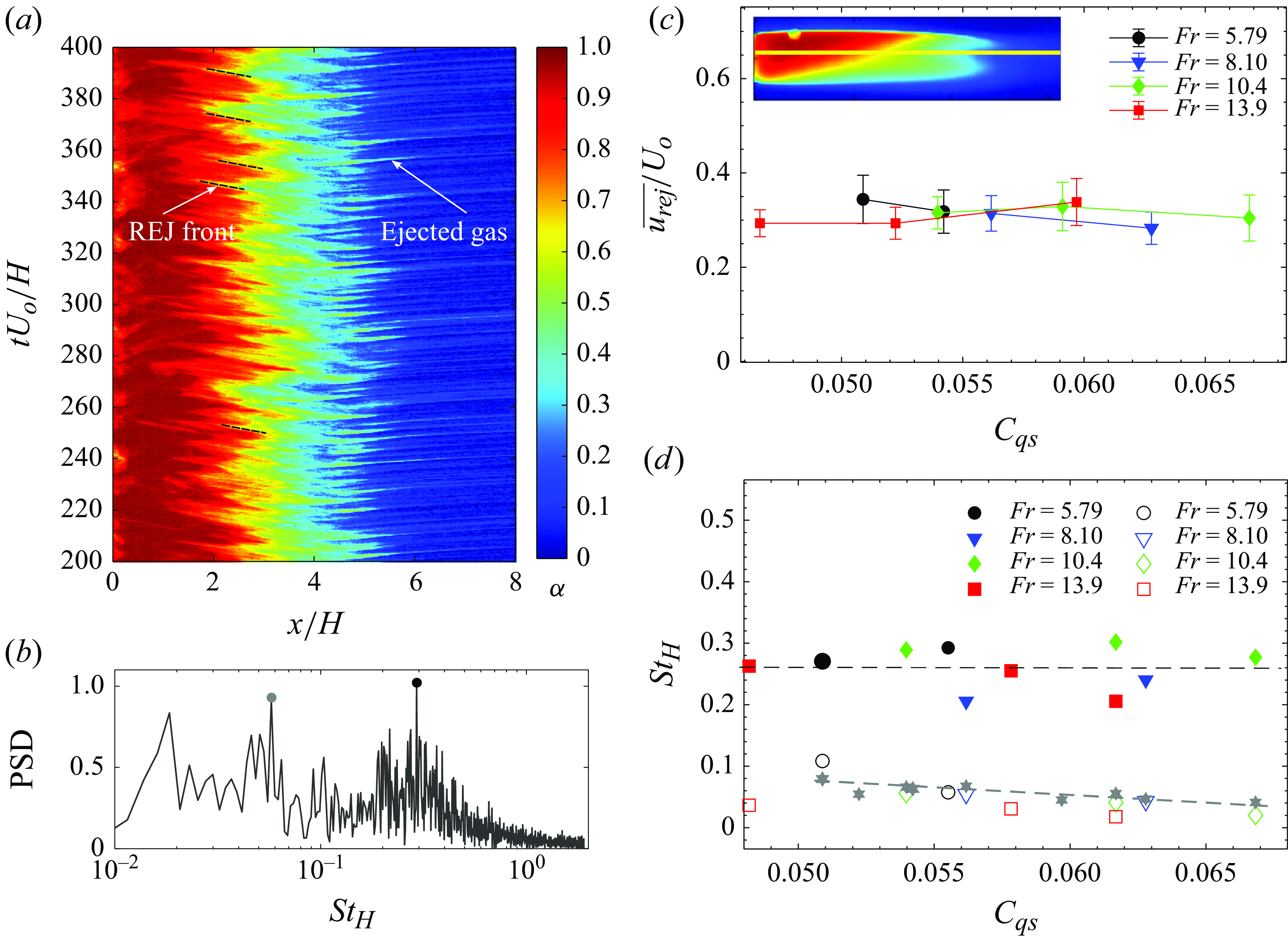
Figure 25. (a) A sample $x{-}t$
diagram showing the evolution of the void fraction for an REJC at
$x{-}t$
diagram showing the evolution of the void fraction for an REJC at $\textit{Fr} = 5.79$
,
$\textit{Fr} = 5.79$
, $C_{qs} = 0.054$
. Examples of the re-entrant flow fronts are indicated by black dashed lines. (b) Power spectral density (PSD) of the void fraction computed from the
$C_{qs} = 0.054$
. Examples of the re-entrant flow fronts are indicated by black dashed lines. (b) Power spectral density (PSD) of the void fraction computed from the $x{-}t$
plot at
$x{-}t$
plot at $X/H \approx$
5, showing two distinct shedding frequencies,
$X/H \approx$
5, showing two distinct shedding frequencies, $St_{H}$
. (c) Re-entrant flow velocity in the laboratory frame of reference estimated from the
$St_{H}$
. (c) Re-entrant flow velocity in the laboratory frame of reference estimated from the $x{-}t$
diagram normalised with inflow velocity (
$x{-}t$
diagram normalised with inflow velocity ( $U_{o}$
) for a range of
$U_{o}$
) for a range of $\textit{Fr}$
and
$\textit{Fr}$
and $C_{qs}$
. (d) Non-dimensional shedding frequency (
$C_{qs}$
. (d) Non-dimensional shedding frequency ( $St_{H}$
) for a range of
$St_{H}$
) for a range of $\textit{Fr}$
and
$\textit{Fr}$
and $C_{qs}$
. Solid markers show the gas ejection frequency due to vortex shedding. Open markers show the gas ejection frequency due to the re-entrant jet impingement. Grey markers (
$C_{qs}$
. Solid markers show the gas ejection frequency due to vortex shedding. Open markers show the gas ejection frequency due to the re-entrant jet impingement. Grey markers ( $\ast$
) show
$\ast$
) show $St$
based on measured kinematics of the re-entrant flow (
$St$
based on measured kinematics of the re-entrant flow ( $L_{c}$
and
$L_{c}$
and $\overline {u_{rej}}$
). The grey dashed line fit to grey markers is given as
$\overline {u_{rej}}$
). The grey dashed line fit to grey markers is given as $St_{H,rej} = 0.2-2.375C_{qs, in}$
.
$St_{H,rej} = 0.2-2.375C_{qs, in}$
.
The characteristics of the re-entrant flow can be estimated from a space–time ( $x{-}t$
) diagram of time-resolved void fraction fields. The
$x{-}t$
) diagram of time-resolved void fraction fields. The $x{-}t$
plot in figure 25(a) shows the void fraction time evolution along the yellow line (
$x{-}t$
plot in figure 25(a) shows the void fraction time evolution along the yellow line ( $y/H \approx- 0.27$
) shown in the inset of figure 25(c). The black dotted lines visualise the liquid REJ fronts inside the cavity, and the ejected gas is indicated by the white arrow in the
$y/H \approx- 0.27$
) shown in the inset of figure 25(c). The black dotted lines visualise the liquid REJ fronts inside the cavity, and the ejected gas is indicated by the white arrow in the $x{-}t$
plot. The velocity of the re-entrant jet front and the convection of the ejected gas are estimated from
$x{-}t$
plot. The velocity of the re-entrant jet front and the convection of the ejected gas are estimated from $x{-}t$
diagrams. The measured REJ front velocity
$x{-}t$
diagrams. The measured REJ front velocity $u_{rej}$
, when normalised with the inflow velocity (
$u_{rej}$
, when normalised with the inflow velocity ( $U_{0}$
), is constant (
$U_{0}$
), is constant ( $\overline {u_{rej}}/U_0 \approx 0.3$
) irrespective of
$\overline {u_{rej}}/U_0 \approx 0.3$
) irrespective of $C_{qs}$
and
$C_{qs}$
and $\textit{Fr}$
as shown in figure 25(c). Strouhal number (
$\textit{Fr}$
as shown in figure 25(c). Strouhal number ( $St_{H} = fH/U_0$
) of the gas ejection frequency,
$St_{H} = fH/U_0$
) of the gas ejection frequency, $f$
, estimated via afast Fourier transform (FFT) of the time signal extracted from the
$f$
, estimated via afast Fourier transform (FFT) of the time signal extracted from the $x{-}t$
plot, is shown in figure 25(d). The FFT was performed on the time signal of the void fraction at a probing point in the wake (
$x{-}t$
plot, is shown in figure 25(d). The FFT was performed on the time signal of the void fraction at a probing point in the wake ( $X/H \approx$
5). Two distinct (dominant) peaks were observed in the spectral density (see figure 25
b) corresponding to two distinct gas ejection mechanisms. These peaks are indicated by grey and black circular markers: gas ejection due to vortex shedding occurs at a roughly constant non-dimensional frequency (
$X/H \approx$
5). Two distinct (dominant) peaks were observed in the spectral density (see figure 25
b) corresponding to two distinct gas ejection mechanisms. These peaks are indicated by grey and black circular markers: gas ejection due to vortex shedding occurs at a roughly constant non-dimensional frequency ( $St_{H,v}\approx 0.27$
). See the frequency peak indicated by the black circular marker in the PSD in figure 25(b). The gas ejection associated with the re-entrant jet displacing the gas occurs at a lower frequency (
$St_{H,v}\approx 0.27$
). See the frequency peak indicated by the black circular marker in the PSD in figure 25(b). The gas ejection associated with the re-entrant jet displacing the gas occurs at a lower frequency ( $St_{H,rej} \lesssim 0.1$
). See the frequency peak indicated by the grey circular marker in the PSD in figure 25(b). The
$St_{H,rej} \lesssim 0.1$
). See the frequency peak indicated by the grey circular marker in the PSD in figure 25(b). The $St$
based on the time taken by the re-entrant jet to impinge on the wedge base (using
$St$
based on the time taken by the re-entrant jet to impinge on the wedge base (using $1/t = \overline {u}_{rej}/L_{c}$
) matches the shedding frequency estimated from the FFT of re-entrant flow-induced gas ejection very well, as shown by the grey filled-star markers in figure 25(d). This suggests a correlation between the re-entrant jet and gas ejection. Additionally, it is observed that
$1/t = \overline {u}_{rej}/L_{c}$
) matches the shedding frequency estimated from the FFT of re-entrant flow-induced gas ejection very well, as shown by the grey filled-star markers in figure 25(d). This suggests a correlation between the re-entrant jet and gas ejection. Additionally, it is observed that $St_{H,rej}$
decreases linearly:
$St_{H,rej}$
decreases linearly: $St_{H,rej} = 0.2-2.375C_{qs, in}$
as
$St_{H,rej} = 0.2-2.375C_{qs, in}$
as $C_{qs}$
increases as shown by a grey dashed line in figure 25(d). This empirical relation is invoked in Appendix B for constructing a simple model for gas ejection.
$C_{qs}$
increases as shown by a grey dashed line in figure 25(d). This empirical relation is invoked in Appendix B for constructing a simple model for gas ejection.
Appendix B. Gas ejection model for transition of REJC to LC
The gas ejection rate due to periodically re-entering liquid flow ( $\dot Q_{out, rej}$
) can be approximated as
$\dot Q_{out, rej}$
) can be approximated as $V_{rej}f_{rej}$
, where
$V_{rej}f_{rej}$
, where $V_{rej}$
and
$V_{rej}$
and $f_{rej}$
are the volume and the frequency of the re-entering flow. The
$f_{rej}$
are the volume and the frequency of the re-entering flow. The $V_{rej}$
can then be approximated as
$V_{rej}$
can then be approximated as $l_{rej}HW/2$
due to the triangular shape of the averaged re-entering flow (see figure 9
c and inset in figure 26
a). The gas ejection can now be expressed as
$l_{rej}HW/2$
due to the triangular shape of the averaged re-entering flow (see figure 9
c and inset in figure 26
a). The gas ejection can now be expressed as $C_{qs, out, rej}$
as per (B1) and rearranged to obtain (B2) using
$C_{qs, out, rej}$
as per (B1) and rearranged to obtain (B2) using $\overline {u_{rej}}/U_0 \approx 0.3$
. Finally, we arrive at (B3) using empirical relations obtained experimentally for
$\overline {u_{rej}}/U_0 \approx 0.3$
. Finally, we arrive at (B3) using empirical relations obtained experimentally for $l_{rej, max}(Fr)/H$
,
$l_{rej, max}(Fr)/H$
, $St_{H,rej}(C_{qs,in})$
in figure 25(d) and figure 22(e), respectively. All the symbols have been explained previously.
$St_{H,rej}(C_{qs,in})$
in figure 25(d) and figure 22(e), respectively. All the symbols have been explained previously.
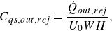 \begin{align}&\qquad\qquad\quad C_{qs, out, rej} = \frac {\dot Q_{out, rej}}{U_{0}WH},\\[-10pt]\nonumber \end{align}
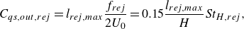 \begin{align}&\quad C_{qs, out, rej} = l_{rej, max} \frac { f_{rej} }{2U_{0}} = 0.15\frac {l_{rej, max}}{H} St_{H,rej},\\[-10pt]\nonumber \end{align}
 \begin{align}& C_{qs, out, rej} = 0.15(0.86 Fr-0.73)(0.2-2.38 C_{qs, in}). \end{align}
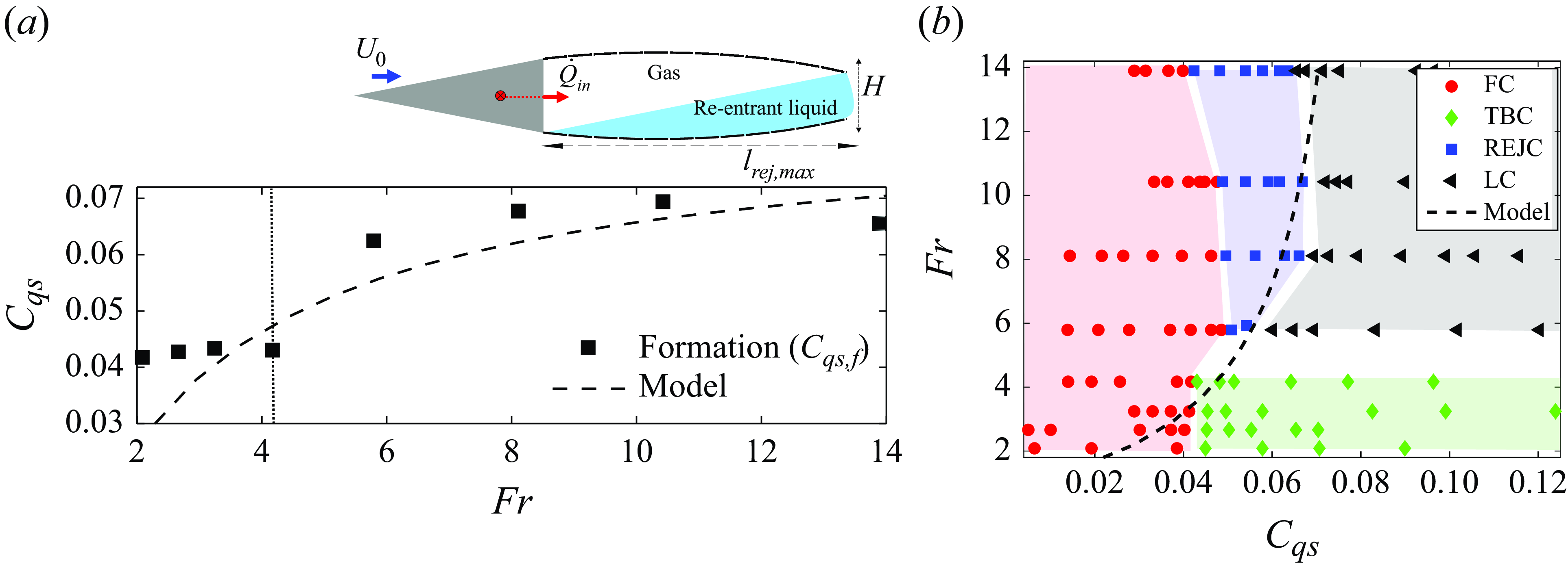
Figure 26. (a)Plot of $C_{qs,f}$
in comparison with the model prediction as a function of
$C_{qs,f}$
in comparison with the model prediction as a function of $\textit{Fr}$
(the black vertical dotted line indicates the
$\textit{Fr}$
(the black vertical dotted line indicates the $\textit{Fr}$
limit where re-entrant flow dictates transition to a supercavity). The inset shows the schematic of the re-entrant flow. (b) Model prediction (
$\textit{Fr}$
limit where re-entrant flow dictates transition to a supercavity). The inset shows the schematic of the re-entrant flow. (b) Model prediction ( $ C_{qs} = C_{qs, out, rej}$
) in the regime map of figure 7.
$ C_{qs} = C_{qs, out, rej}$
) in the regime map of figure 7.
The locus of $C_{qs, in}$
for which
$C_{qs, in}$
for which $C_{qs, in} \gt C_{qs, out, rej}$
is shown by the black dashed line in figure 26. It agrees well with
$C_{qs, in} \gt C_{qs, out, rej}$
is shown by the black dashed line in figure 26. It agrees well with $C_{qs, f}$
at higher
$C_{qs, f}$
at higher $\textit{Fr}$
(
$\textit{Fr}$
( $\gt$
4.17), suggesting that gas ejection, i.e. displaced due to re-entrant flow, accounts for the majority of the gas ejection, preventing the ventilated cavity from growing longer to an LC. Thus, if
$\gt$
4.17), suggesting that gas ejection, i.e. displaced due to re-entrant flow, accounts for the majority of the gas ejection, preventing the ventilated cavity from growing longer to an LC. Thus, if $C_{qs, in} \gt C_{qs, out, rej}$
, the cavity will experience net growth to an LC from an REJC as it can overcome the gas ejection due to the re-entering liquid flow. Furthermore, at low
$C_{qs, in} \gt C_{qs, out, rej}$
, the cavity will experience net growth to an LC from an REJC as it can overcome the gas ejection due to the re-entering liquid flow. Furthermore, at low $\textit{Fr}$
(
$\textit{Fr}$
( ${\lt } 4.17$
), the predicted ejection due to the re-entrant flow is less than the measured ejection (
${\lt } 4.17$
), the predicted ejection due to the re-entrant flow is less than the measured ejection ( $C_{qs,f}$
). This suggests that the re-entrant flow in such cavities is mild and does not account for the majority of gas leakage. Instead, interfacial perturbation and the spanwise vortex ejection cause the majority of the gas leakage, consistent with our experimental observations.
$C_{qs,f}$
). This suggests that the re-entrant flow in such cavities is mild and does not account for the majority of gas leakage. Instead, interfacial perturbation and the spanwise vortex ejection cause the majority of the gas leakage, consistent with our experimental observations.


 Open access