


1. Introduction
1.1. Two-fluid–structure interaction
The fluid–structure interaction problem involving single-phase flow past a stationary circular cylinder has remained one of the central problems in fluid dynamics for an extended period (Strouhal Reference Strouhal1878; von Kármán & Rubach Reference von Kármán and Rubach1912; Roshko Reference Roshko1955; Williamson Reference Williamson1996). In the case of isothermal Newtonian fluids, the flow characteristics arising from this problem are governed by a single control parameter – the Reynolds number
 $ Re =\mathcal {O}{ (\text {inertial forces} )}/\mathcal {O}{ (\text {viscous forces} )}$
. The continuing research on vortex-induced vibrations (Williamson & Govardhan Reference Williamson and Govardhan2004) in such bluff-body flows, caused by periodic shedding of vortices, has paved the way for innovative energy harvesting applications (Lee et al. Reference Lee, Qi, Zhou and Lua2019; Joy et al. Reference Joy, Joshi, Narendran and Ghoshal2023).
$ Re =\mathcal {O}{ (\text {inertial forces} )}/\mathcal {O}{ (\text {viscous forces} )}$
. The continuing research on vortex-induced vibrations (Williamson & Govardhan Reference Williamson and Govardhan2004) in such bluff-body flows, caused by periodic shedding of vortices, has paved the way for innovative energy harvesting applications (Lee et al. Reference Lee, Qi, Zhou and Lua2019; Joy et al. Reference Joy, Joshi, Narendran and Ghoshal2023).
Over time, numerous physics-rich variants of this canonical flow problem have surfaced. Examples include flow around an oscillating cylinder (Hourigan Reference Hourigan2021), flow past a fixed cylinder with a superhydrophobic surface (Sooraj et al. Reference Sooraj, Ramagya, Khan, Sharma and Agrawal2020), confined viscoelastic flow across twin cylinders (Hopkins, Haward & Shen Reference Hopkins, Haward and Shen2021) and many more. In a similar fashion, in our study, we focus on a spin-off of this classical fluid–structure interaction problem. We perform simulations of a two-fluid–structure interaction (tFSI) problem involving liquid–gas flow over a stationary cylinder. The cylinder is completely immersed in the flowing liquid phase and is positioned in close proximity to the horizontal liquid–gas interface. The introduction of a free surface in the form of a liquid–gas interface brings about several intriguing effects via the interaction between disturbance flow originating from the presence of a circular cylinder, buoyancy, viscosity contrast and surface tension. Thus, unlike the traditional flow past a cylinder arrangement, the present tFSI problem is characterised by a multi-dimensional control parameter space. Furthermore, the current flow configuration is also representative of a typical arrangement encountered in offshore structures (Reichl, Hourigan & Thompson Reference Reichl, Hourigan and Thompson2005; Zhao et al. Reference Zhao, Wang, Zhu, Ping, Bao, Zhou, Cao and Cui2021).
In one of the first experimental studies, Sheridan, Lin & Rockwell (Reference Sheridan, Lin and Rockwell1997) investigated the dynamics of uniform flow around a stationary cylinder positioned beneath a free surface that separates air and water. Their study specifically examined flows with
 $Re \sim \mathcal {O}{ (1000 )}$
. In addition to
$Re \sim \mathcal {O}{ (1000 )}$
. In addition to
 $ Re$
, they introduced the Froude number
$ Re$
, they introduced the Froude number
 $Fr^{2} = \mathcal {O}{ (\text {inertial forces} )}/\mathcal {O}{ (\text {gravitational forces} )}$
and the submergence depth
$Fr^{2} = \mathcal {O}{ (\text {inertial forces} )}/\mathcal {O}{ (\text {gravitational forces} )}$
and the submergence depth
 $h/D$
, representing the gap between the cylinder, with a diameter of
$h/D$
, representing the gap between the cylinder, with a diameter of
 $D$
, and the free surface at height
$D$
, and the free surface at height
 $h$
. Parameters
$h$
. Parameters
 $ Fr$
and
$ Fr$
and
 $h/D$
are relevant for quantifying the dynamics of the free surface and its interaction with the cylinder wake. Their particle image velocimetry uncovered two distinct features within the wake region when the air–water interface was almost undistorted (low
$h/D$
are relevant for quantifying the dynamics of the free surface and its interaction with the cylinder wake. Their particle image velocimetry uncovered two distinct features within the wake region when the air–water interface was almost undistorted (low
 $ Fr$
values) and located close to the cylinder surface. First, a stable jet-like flow emanated from the gap between the top of the cylinder and the free surface. Second, a noticeable downward bending of the mixing layer occurred at the bottom of the cylinder. Additionally, specific
$ Fr$
values) and located close to the cylinder surface. First, a stable jet-like flow emanated from the gap between the top of the cylinder and the free surface. Second, a noticeable downward bending of the mixing layer occurred at the bottom of the cylinder. Additionally, specific
 $\{Fr, h/D\}$
combinations were found to induce the appearance of a wavy air–water interface and small-scale wave breaking. Nevertheless, the core of their discussion primarily centred on the direct observations of vorticity dynamics in the immediate vicinity of the cylinder, spanning approximately three times the cylinder diameter in the downstream direction.
$\{Fr, h/D\}$
combinations were found to induce the appearance of a wavy air–water interface and small-scale wave breaking. Nevertheless, the core of their discussion primarily centred on the direct observations of vorticity dynamics in the immediate vicinity of the cylinder, spanning approximately three times the cylinder diameter in the downstream direction.
Subsequently, several groups performed two-dimensional numerical studies of flow set-ups involving circular (Reichl et al. Reference Reichl, Hourigan and Thompson2005; Colagrossi et al. Reference Colagrossi, Nikolov, Durante, Marrone and Souto-Iglesias2019; González-Gutierrez et al. Reference González-Gutierrez, Gimenez and Ferrer2019; Wang et al. Reference Wang, Mao, Song and Tian2021; De Vita et al. Reference De Vita, De Lillo, Verzicco and Onorato2021; Lin & Yao Reference Lin and Yao2023), elliptic (Subburaj, Khandelwal & Vengadesan Reference Subburaj, Khandelwal and Vengadesan2018) and square (Karmakar & Saha Reference Karmakar and Saha2020) cylinders for relatively low Reynolds numbers
 $ (Re \leqslant 250 )$
. Notably, these two-dimensional simulations exhibit flow features that are qualitatively similar to those observed in the experiments of Sheridan et al. (Reference Sheridan, Lin and Rockwell1997). Using volume-of-fluid simulations, Reichl et al. (Reference Reichl, Hourigan and Thompson2005) mapped the no-shedding and shedding wake states for different combinations of
$ (Re \leqslant 250 )$
. Notably, these two-dimensional simulations exhibit flow features that are qualitatively similar to those observed in the experiments of Sheridan et al. (Reference Sheridan, Lin and Rockwell1997). Using volume-of-fluid simulations, Reichl et al. (Reference Reichl, Hourigan and Thompson2005) mapped the no-shedding and shedding wake states for different combinations of
 $ Fr$
and
$ Fr$
and
 $h/D$
. The presence of the nearby free surface at the lower
$h/D$
. The presence of the nearby free surface at the lower
 $ Fr$
and
$ Fr$
and
 $h/D$
values dampens the negative vorticity originating from the upper half of the cylinder due to the reduced flow in the gap between the cylinder and the free surface. The resulting negative vorticity rapidly dissipates in the wake region, leading to the absence of vortex shedding. Furthermore, when the free surface begins to deform at relatively larger values of
$h/D$
values dampens the negative vorticity originating from the upper half of the cylinder due to the reduced flow in the gap between the cylinder and the free surface. The resulting negative vorticity rapidly dissipates in the wake region, leading to the absence of vortex shedding. Furthermore, when the free surface begins to deform at relatively larger values of
 $ Fr$
, interfacial circulation counteracts the negative vorticity in the liquid phase. This, once again, leads to a cylinder wake devoid of alternating vortices.
$ Fr$
, interfacial circulation counteracts the negative vorticity in the liquid phase. This, once again, leads to a cylinder wake devoid of alternating vortices.
Reichl et al. (Reference Reichl, Hourigan and Thompson2005) also observed the development of curved areas on the free surface near the cylinder despite the
 $ Fr$
values being well below unity, i.e. subcritical flow. Upon examining the local Froude number in the gap above the cylinder surface, they found the flow nearing the critical condition with the local Froude number approaching unity. This observation explains the deviation of the free surface from the flat state, which was also evident in the experiments of Sheridan et al. (Reference Sheridan, Lin and Rockwell1997). A detailed discussion about the onset of vortex shedding and free-surface deformation was presented by González-Gutierrez et al. (Reference González-Gutierrez, Gimenez and Ferrer2019) using global stability analysis. It was shown that for elevated Froude numbers
$ Fr$
values being well below unity, i.e. subcritical flow. Upon examining the local Froude number in the gap above the cylinder surface, they found the flow nearing the critical condition with the local Froude number approaching unity. This observation explains the deviation of the free surface from the flat state, which was also evident in the experiments of Sheridan et al. (Reference Sheridan, Lin and Rockwell1997). A detailed discussion about the onset of vortex shedding and free-surface deformation was presented by González-Gutierrez et al. (Reference González-Gutierrez, Gimenez and Ferrer2019) using global stability analysis. It was shown that for elevated Froude numbers
 $ (2 \leqslant Fr \leqslant 2.5 )$
, the presence of a nearby free surface makes the flow more susceptible to instability, thereby bringing down the critical Reynolds number compared with the traditional single-phase flow across a circular cylinder. Conversely, this trend is reversed for
$ (2 \leqslant Fr \leqslant 2.5 )$
, the presence of a nearby free surface makes the flow more susceptible to instability, thereby bringing down the critical Reynolds number compared with the traditional single-phase flow across a circular cylinder. Conversely, this trend is reversed for
 $ {Fr}$
values below unity.
$ {Fr}$
values below unity.
Besides flow states with and without vortex streets, Sheridan et al. (Reference Sheridan, Lin and Rockwell1997) and Reichl et al. (Reference Reichl, Hourigan and Thompson2005) noted the existence of a metastable wake state in their studies, wherein the liquid jet emerging from the gap between the cylinder and the free surface undergoes oscillations. Later, Colagrossi et al. (Reference Colagrossi, Nikolov, Durante, Marrone and Souto-Iglesias2019) monitored the variation of the lift force experienced by the cylinder in the metastable state for substantially longer times. The time history indicated irregular oscillations in the lift force with a complete absence of vortex shedding during certain time intervals. Moreover, Colagrossi et al. (Reference Colagrossi, Nikolov, Durante, Marrone and Souto-Iglesias2019) showed that such a lift force signal contains one dominant frequency associated with the vortex shedding and an additional order-of-magnitude-smaller frequency associated with the oscillations of the jet. Interestingly, such metastable states also involve the entrainment of air (or gas) bubbles, as seen in Reichl et al. (Reference Reichl, Hourigan and Thompson2005) and Colagrossi et al. (Reference Colagrossi, Nikolov, Durante, Marrone and Souto-Iglesias2019). Bubble formation through free-surface breakup was also observed by Subburaj et al. (Reference Subburaj, Khandelwal and Vengadesan2018) for an elliptic cylinder and González-Gutierrez et al. (Reference González-Gutierrez, Gimenez and Ferrer2019) for a circular cylinder. However, prior numerical studies did not account for surface tension in their simulations, which may alter the interface dynamics.
Only recently, Guo et al. (Reference Guo, Ji, Han, Liu, Wu and Kuai2023) incorporated surface tension in free-surface simulations. Their work focused on a rotating cylinder near the free surface for
 $ {Fr}$
values up to
$ {Fr}$
values up to
 $0.5$
, wherein they reported the entrainment of air bubbles in the cylinder wake. These entrained air bubbles were found to vary from one to two orders of magnitude smaller than the cylinder diameter. In the present work, we explore flow physics using a more realistic set-up involving surface tension. Particularly for high
$0.5$
, wherein they reported the entrainment of air bubbles in the cylinder wake. These entrained air bubbles were found to vary from one to two orders of magnitude smaller than the cylinder diameter. In the present work, we explore flow physics using a more realistic set-up involving surface tension. Particularly for high
 $ {Fr}\ ({\geqslant }1 )$
cases investigated in our study, where the liquid–gas interface starts to deform significantly and break, the inclusion of surface tension is crucial. The presence of surface tension introduces the Weber number
$ {Fr}\ ({\geqslant }1 )$
cases investigated in our study, where the liquid–gas interface starts to deform significantly and break, the inclusion of surface tension is crucial. The presence of surface tension introduces the Weber number
 $ {We} = \mathcal {O}{ (\text {inertial forces} )}/\mathcal {O}{ (\text {surface tension forces} )}$
and Bond number
$ {We} = \mathcal {O}{ (\text {inertial forces} )}/\mathcal {O}{ (\text {surface tension forces} )}$
and Bond number
 $ {Bo} = \mathcal {O}{ (\text {gravitational forces} )}/\mathcal {O}{ (\text {surface tension forces} )}$
, providing a complete description of the current tFSI problem, along with the parameters
$ {Bo} = \mathcal {O}{ (\text {gravitational forces} )}/\mathcal {O}{ (\text {surface tension forces} )}$
, providing a complete description of the current tFSI problem, along with the parameters
 $h/D$
and
$h/D$
and
 $ {Re}$
. Also, note that
$ {Re}$
. Also, note that
 $ {Fr}^{2} = {We}/ {Bo}$
.
$ {Fr}^{2} = {We}/ {Bo}$
.
Apart from low-Reynolds-number free-surface flows across cylinders, there have also been some recent efforts to realise high-Reynolds-number scenarios in numerical studies. Zhao et al. (Reference Zhao, Wang, Zhu, Ping, Bao, Zhou, Cao and Cui2021) utilised large-eddy simulations for Re and Fr values in a range similar to that investigated by Sheridan et al. (Reference Sheridan, Lin and Rockwell1997). They noted that at sufficiently high enough Fr, the mean free-surface elevation in the downstream region of the cylinder becomes significant, reaching
 $10\,\%$
of the cylinder diameter for
$10\,\%$
of the cylinder diameter for
 $ {Fr} =0.6$
in their study. Later, Alzabari, Wilson & Ouro (Reference Alzabari, Wilson and Ouro2023) conducted large-eddy simulations to gain insights into vortex shedding behind a circular cylinder in shallow-water flows. Here, the interaction between ground vortices and those shed from the cylinder becomes important, leading to modifications in turbulent mixing and downstream free-surface dynamics.
$ {Fr} =0.6$
in their study. Later, Alzabari, Wilson & Ouro (Reference Alzabari, Wilson and Ouro2023) conducted large-eddy simulations to gain insights into vortex shedding behind a circular cylinder in shallow-water flows. Here, the interaction between ground vortices and those shed from the cylinder becomes important, leading to modifications in turbulent mixing and downstream free-surface dynamics.
In addition to rigid cylinders of various shapes, free-surface flows past spheres (Sareen et al. Reference Sareen, Zhao, Sheridan, Hourigan and Thompson2018; Chizfahm et al. Reference Chizfahm, Joshi and Jaiman2021; Rajamuni et al. Reference Rajamuni, Hourigan and Thompson2021; De Vita et al. Reference De Vita, De Lillo, Verzicco and Onorato2021; Hunt et al. Reference Hunt, Zhao, Silver, Yan, Bazilevs and Harris2023), flat plates (Hofman Reference Hofman1993; Díaz-Ojeda et al. Reference Díaz-Ojeda, Huera-Huarte and González-Gutiérrez2019; Hu et al. Reference Hu, Liu, Zhao and Hu2023), hydrofoils (Iafrati & Campana Reference Iafrati and Campana2005) and transom sterns (Hendrickson et al. Reference Hendrickson, Weymouth, Yu and Yue2019; Yang et al. Reference Yang, Hu, Liu, Gao and Hu2023) are also focus points of ongoing work.
Our previous discussion on existing research showcases a growing interest in free-surface/two-phase flows across bluff bodies. However, it is apparent that earlier low-Reynolds-number numerical simulations on free-surface flow around a submerged cylinder primarily concentrated on structural loads and vorticity dynamics near the cylinder and weakly deformed interface. Moreover, occasional breakup events in these studies lacked the restoring force exerted by surface tension, i.e.
 $ {We} =\infty$
. The present study focuses on the following key aspects to expand upon previous research: (a) incorporating finite surface tension into the numerical formulation and quantifying its influence on interfacial phenomena; (b) systematically mapping various regimes of interface dynamics and associated wake structures for different values of the parameters set
$ {We} =\infty$
. The present study focuses on the following key aspects to expand upon previous research: (a) incorporating finite surface tension into the numerical formulation and quantifying its influence on interfacial phenomena; (b) systematically mapping various regimes of interface dynamics and associated wake structures for different values of the parameters set
 $\{h/D$
, Re, We, Bo}; (c) presenting a unified discussion on the hydrodynamic lift force experienced by the cylinder, considering its interplay with the shape and deformability of the adjacent liquid–gas interface; (d) characterising the wave patterns that emerge on the liquid–gas surface due to the presence of the cylinder; and (e) examining the mechanisms responsible for gas entrainment in the cylinder’s wake, alongside a detailed analysis of the Lagrangian statistics associated with the entrained gas bubbles.
$\{h/D$
, Re, We, Bo}; (c) presenting a unified discussion on the hydrodynamic lift force experienced by the cylinder, considering its interplay with the shape and deformability of the adjacent liquid–gas interface; (d) characterising the wave patterns that emerge on the liquid–gas surface due to the presence of the cylinder; and (e) examining the mechanisms responsible for gas entrainment in the cylinder’s wake, alongside a detailed analysis of the Lagrangian statistics associated with the entrained gas bubbles.
The structure of the rest of the article is organised as follows. Next, in § 2, we introduce our flow set-up, computational framework and parametric details. Following this, in § 3, we analyse our numerical findings and discuss the underlying physics of the present tFSI problem. First, we examine the overall trends in the dynamics of the liquid–gas interface and vorticity field alongside the hydrodynamic lift force acting on the rigid cylinder. Subsequently, we take a closer look at interesting flow features in our parameter space, such as wave formation and bubble entrainment. We also comment on the bubble entrainment phenomenon in a three-dimensional setting by considering an extreme scenario with the lowest submergence depth in our parameter space. Finally, we wrap up our discussion with concluding remarks in § 4. A rigorous discussion on the benchmarking and grid convergence of our two-dimensional flow solver is provided in Appendix A.
2. Methods
The discussion of numerical techniques in this section pertains exclusively to the two-dimensional simulation results presented in §§ 3.1–3.5. The numerical framework for the three-dimensional case in § 3.6 will be detailed later within that subsection, alongside the results.
2.1. Flow domain
The diagram showcasing the geometry of our flow domain is illustrated in figure 1. We consider a square domain of size
 $L$
, partially filled with a liquid of density
$L$
, partially filled with a liquid of density
 $\rho _{1}$
and dynamic viscosity
$\rho _{1}$
and dynamic viscosity
 $\mu _{1}$
. The remainder of the domain contains a gas of density
$\mu _{1}$
. The remainder of the domain contains a gas of density
 $\rho _{2}$
and dynamic viscosity
$\rho _{2}$
and dynamic viscosity
 $\mu _{2}$
. The box size
$\mu _{2}$
. The box size
 $L$
and property ratios (
$L$
and property ratios (
 $\rho _{1}/\rho _{2}$
and
$\rho _{1}/\rho _{2}$
and
 $\mu _{1}/\mu _{2}$
) are provided later in this section. The interface (free surface) separating liquid and gas phases has surface tension
$\mu _{1}/\mu _{2}$
) are provided later in this section. The interface (free surface) separating liquid and gas phases has surface tension
 $\sigma$
. The base state of the system corresponds to a steady uniform flow in the positive
$\sigma$
. The base state of the system corresponds to a steady uniform flow in the positive
 $x$
direction with a velocity magnitude
$x$
direction with a velocity magnitude
 $U$
. Note that the uniform flow within the liquid phase also drags the gas phase with it, giving rise to a flowing gas layer adjacent to the liquid–gas interface, i.e. the two-phase mixing layer.
$U$
. Note that the uniform flow within the liquid phase also drags the gas phase with it, giving rise to a flowing gas layer adjacent to the liquid–gas interface, i.e. the two-phase mixing layer.

Figure 1. Computational set-up for free-surface flow past a stationary circular cylinder. The incoming unidirectional uniform base flow impacts the cylinder, inducing flow disturbances in the downstream region. Consequently, these disturbances may perturb the flat liquid–gas interface and the flowing gas layer in the interfacial region.
The base flow entering the computational domain is disturbed by the rigid circular cylinder of diameter
 $D$
, as shown in figure 1. Our objective is to examine the flow perturbations resulting from the interaction between the flowing liquid and cylinder and their impact on the dynamics of the liquid–gas interface. The cylinder is located at a distance
$D$
, as shown in figure 1. Our objective is to examine the flow perturbations resulting from the interaction between the flowing liquid and cylinder and their impact on the dynamics of the liquid–gas interface. The cylinder is located at a distance
 $10D$
from the inlet and
$10D$
from the inlet and
 $h$
from the initially flat liquid–gas interface. The top and bottom boundaries of our computational domain are treated as stress-free walls, i.e. the free-slip condition. The inlet boundary condition is applied to the left edge of the domain, allowing only the influx of the liquid phase with a prescribed velocity
$h$
from the initially flat liquid–gas interface. The top and bottom boundaries of our computational domain are treated as stress-free walls, i.e. the free-slip condition. The inlet boundary condition is applied to the left edge of the domain, allowing only the influx of the liquid phase with a prescribed velocity
 $U$
(Karmakar & Saha Reference Karmakar and Saha2020; Guo et al. Reference Guo, Ji, Han, Liu, Wu and Kuai2023), while the interface elevation is fixed at a height
$U$
(Karmakar & Saha Reference Karmakar and Saha2020; Guo et al. Reference Guo, Ji, Han, Liu, Wu and Kuai2023), while the interface elevation is fixed at a height
 $h$
(see figure 1). This approach effectively models free-surface flow experiments commonly conducted in water tunnels (Sareen et al. Reference Sareen, Zhao, Sheridan, Hourigan and Thompson2018; Hunt et al. Reference Hunt, Zhao, Silver, Yan, Bazilevs and Harris2023). At the right edge of the domain, an outflow boundary condition is implemented. This involves prescribing a Neumann boundary condition (zero normal gradient) for both the velocity
$h$
(see figure 1). This approach effectively models free-surface flow experiments commonly conducted in water tunnels (Sareen et al. Reference Sareen, Zhao, Sheridan, Hourigan and Thompson2018; Hunt et al. Reference Hunt, Zhao, Silver, Yan, Bazilevs and Harris2023). At the right edge of the domain, an outflow boundary condition is implemented. This involves prescribing a Neumann boundary condition (zero normal gradient) for both the velocity
 $\boldsymbol {u}$
and the volume fraction field
$\boldsymbol {u}$
and the volume fraction field
 $C$
, along with a Dirichlet boundary condition (set to zero) for the pressure
$C$
, along with a Dirichlet boundary condition (set to zero) for the pressure
 $p$
. Note that the present implementation of the outflow boundary condition is realised by reshaping gravity as an interfacial force (Wroniszewski, Verschaeve & Pedersen Reference Wroniszewski, Verschaeve and Pedersen2014; Popinet Reference Popinet2018).
$p$
. Note that the present implementation of the outflow boundary condition is realised by reshaping gravity as an interfacial force (Wroniszewski, Verschaeve & Pedersen Reference Wroniszewski, Verschaeve and Pedersen2014; Popinet Reference Popinet2018).
The validation study presented in Appendix A demonstrates that the implemented outflow boundary condition yields results consistent with those of a previously published numerical study that utilises a sponge region at the outlet. In our subsequent discussion in § 3, we adopt a computational domain that is twice the size of the one used in the validation study, minimising numerical artifacts associated with the outflow boundary condition. Additionally, we exclude the downstream region within
 $20D$
from the outlet from our analysis. As an additional verification, we also confirmed the consistency of our results using an alternative formulation that employs a coarser mesh at the outlet to artificially under-resolve flow structures, effectively functioning as a sponge region.
$20D$
from the outlet from our analysis. As an additional verification, we also confirmed the consistency of our results using an alternative formulation that employs a coarser mesh at the outlet to artificially under-resolve flow structures, effectively functioning as a sponge region.
2.2. Conservation laws and computational implementation
Typically, computer simulations of multi-fluid problems involve independently solving the Navier–Stokes equations for each fluid component. The solutions acquired for individual fluid components must be matched at all fluid–fluid interfaces using the appropriate kinematic and dynamic boundary conditions. In our study, we incorporate the one-fluid formulation (Juric & Tryggvason Reference Juric and Tryggvason1998; Trujillo Reference Trujillo2021), which employs only one set of conservation laws for the entire computational domain in figure 1. The one-fluid approach is facilitated by reshaping surface tension as a body force (Brackbill, Kothe & Zemach Reference Brackbill, Kothe and Zemach1992), which vanishes in regions away from the fluid–fluid interface and thereby implicitly capturing the Laplace pressure jump across the interface. Following this, we obtain the flow continuity equation
 \begin{eqnarray} \nabla {\cdot }\boldsymbol {u}=0 \end{eqnarray}
and the momentum conservation equation
 \begin{eqnarray} \rho \left (\frac {\partial \boldsymbol {u}}{\partial t}+\boldsymbol {u}{\cdot }\nabla \boldsymbol {u}\right )=-\nabla p + \nabla {\cdot }\left [\mu \left (\nabla \boldsymbol {u}+\left (\nabla \boldsymbol {u}\right )^{T}\right )\right ] + \rho \boldsymbol {g}+\sigma \kappa \delta _{s}\boldsymbol {n}, \end{eqnarray}
where
 $\boldsymbol {u}$
,
$\boldsymbol {u}$
,
 $t$
,
$t$
,
 $p$
,
$p$
,
 $\boldsymbol {g} =\langle 0, g \rangle$
,
$\boldsymbol {g} =\langle 0, g \rangle$
,
 $\kappa =\nabla {\cdot }\boldsymbol {n}$
,
$\kappa =\nabla {\cdot }\boldsymbol {n}$
,
 $\delta _{s}$
and
$\delta _{s}$
and
 $\boldsymbol {n}$
denote the velocity vector, time, pressure, vector for the gravitational acceleration (see figure 1), interface curvature, interface delta function and interface normal, respectively.
$\boldsymbol {n}$
denote the velocity vector, time, pressure, vector for the gravitational acceleration (see figure 1), interface curvature, interface delta function and interface normal, respectively.
In addition to the time evolution of the flow field, we also need to track the movement of the liquid–gas interface shown in figure 1. To accomplish this, we rely on the volume-of-fluid (VOF) framework (Hirt & Nichols Reference Hirt and Nichols1981). The VOF method utilises the volume fraction field
 $C{ (\boldsymbol {x},t )}$
to detect liquid and gas phases in figure 1:
$C{ (\boldsymbol {x},t )}$
to detect liquid and gas phases in figure 1:
 $C{=}1$
for liquid and
$C{=}1$
for liquid and
 $0$
for gas. After each simulation time step,
$0$
for gas. After each simulation time step,
 $C$
is transported using the background flow field
$C$
is transported using the background flow field
 $\boldsymbol {u}$
obtained from (2.1)–(2.2):
$\boldsymbol {u}$
obtained from (2.1)–(2.2):
 \begin{eqnarray} \frac {\partial C}{\partial t}+\boldsymbol {u}{\cdot }\nabla C=0. \end{eqnarray}
Moreover, the fluid density
 $\rho$
in (2.2) is calculated using the weighted average,
$\rho$
in (2.2) is calculated using the weighted average,
 $\rho {=}C\rho _{1}{+}{ (1{-}C )}\rho _{2}$
, whereas the dynamic viscosity
$\rho {=}C\rho _{1}{+}{ (1{-}C )}\rho _{2}$
, whereas the dynamic viscosity
 $\mu$
follows the harmonic mean,
$\mu$
follows the harmonic mean,
 $\mu ^{-1}{=}C\mu ^{-1}_{1}{+}{ (1{-}C )}\mu ^{-1}_{2}$
. In the context of the current liquid–gas system with significant viscosity contrast, opting for the harmonic mean is more suitable (Tryggvason, Scardovelli & Zaleski Reference Tryggvason, Scardovelli and Zaleski2011; Fudge, Cimpeanu & Castrejón-Pita Reference Fudge, Cimpeanu and Castrejón-Pita2021). For interested readers, we highlight that other equally effective interface capturing methods are also available, such as level set (Gibou, Fedkiw & Osher Reference Gibou, Fedkiw and Osher2018) and phase field (Patel & Stark Reference Patel and Stark2023) techniques.
$\mu ^{-1}{=}C\mu ^{-1}_{1}{+}{ (1{-}C )}\mu ^{-1}_{2}$
. In the context of the current liquid–gas system with significant viscosity contrast, opting for the harmonic mean is more suitable (Tryggvason, Scardovelli & Zaleski Reference Tryggvason, Scardovelli and Zaleski2011; Fudge, Cimpeanu & Castrejón-Pita Reference Fudge, Cimpeanu and Castrejón-Pita2021). For interested readers, we highlight that other equally effective interface capturing methods are also available, such as level set (Gibou, Fedkiw & Osher Reference Gibou, Fedkiw and Osher2018) and phase field (Patel & Stark Reference Patel and Stark2023) techniques.
To incorporate (2.1)–(2.3) into our numerical simulations, we employ the open-source finite-volume flow solver Basilisk (Popinet & Collaborators Reference Popinet2013–2024). Basilisk utilises the classical time-splitting projection method (Chorin Reference Chorin1969) along with II-order schemes for the spatial gradients. Furthermore, the viscous term in the momentum conservation (2.2) is computed implicitly, and the II-order Bell–Colella–Glaz unsplit upwind scheme (Bell, Colella & Glaz Reference Bell, Colella and Glaz1989) is incorporated for the velocity advection term
 $\boldsymbol {u}^{n+({1}/{2})}{\cdot }\nabla \boldsymbol {u}^{n+ ({1}/{2})}$
, where the superscript
$\boldsymbol {u}^{n+({1}/{2})}{\cdot }\nabla \boldsymbol {u}^{n+ ({1}/{2})}$
, where the superscript
 $n+({1}/{2})$
indicates the temporal discretisation (Popinet Reference Popinet2009). The interface curvature
$n+({1}/{2})$
indicates the temporal discretisation (Popinet Reference Popinet2009). The interface curvature
 $\kappa$
required for the surface tension body force in (2.2) is obtained using the height function approach (Popinet Reference Popinet2009). Also, the well-balanced implementation of the surface tension force (Popinet Reference Popinet2018) ensures the mitigation of spurious currents in our simulations. Finally, the advection of the volume fraction field
$\kappa$
required for the surface tension body force in (2.2) is obtained using the height function approach (Popinet Reference Popinet2009). Also, the well-balanced implementation of the surface tension force (Popinet Reference Popinet2018) ensures the mitigation of spurious currents in our simulations. Finally, the advection of the volume fraction field
 $C$
in (2.3) is performed using a piecewise-linear geometrical VOF scheme (Scardovelli & Zaleski Reference Scardovelli and Zaleski1999).
$C$
in (2.3) is performed using a piecewise-linear geometrical VOF scheme (Scardovelli & Zaleski Reference Scardovelli and Zaleski1999).
The last aspect we need to address in our framework is the treatment of the curved immersed boundary corresponding to the stationary solid cylinder shown in figure 1. This is not straightforward since all variables in (2.1)–(2.3) are defined on a Cartesian grid. One of the popular approaches is to represent immersed boundaries using Lagrangian markers and then couple them with the background Cartesian grid (Patel & Stark Reference Patel and Stark2021; Zhu et al. Reference Zhu, Chen, Chong, Lohse and Verzicco2024). While this method is particularly effective for scenarios involving moving immersed boundaries, for our current set-up with a stationary body, we follow the VOF-based cut-cell method (Popinet Reference Popinet2003).
This approach introduces an auxiliary volume fraction field
 $\alpha { (\boldsymbol {x} )}$
to distinguish between solid and fluid regions:
$\alpha { (\boldsymbol {x} )}$
to distinguish between solid and fluid regions:
 $\alpha {=}0$
for solid and
$\alpha {=}0$
for solid and
 $1$
for fluid. For mixed control volumes with
$1$
for fluid. For mixed control volumes with
 $0 \lt \alpha \lt 1$
, i.e. the cut cells, computations of gradients and fluxes are adjusted to account for the presence of the solid boundary within the control volume (Johansen & Colella Reference Johansen and Colella1998; Popinet Reference Popinet2003), thereby enforcing the no-slip boundary condition on the surface of the cylinder. The discrete representation of the solid–fluid boundary within control volumes is achieved through piecewise linear reconstruction. Note that the liquid–gas interface remains separate from the cylinder for all the cases investigated in the present work. Thus, modelling of three-phase (solid–liquid–gas) contact line dynamics is not required. Nonetheless, these specific cases are intriguing and will be investigated separately in the subsequent part of this study.
$0 \lt \alpha \lt 1$
, i.e. the cut cells, computations of gradients and fluxes are adjusted to account for the presence of the solid boundary within the control volume (Johansen & Colella Reference Johansen and Colella1998; Popinet Reference Popinet2003), thereby enforcing the no-slip boundary condition on the surface of the cylinder. The discrete representation of the solid–fluid boundary within control volumes is achieved through piecewise linear reconstruction. Note that the liquid–gas interface remains separate from the cylinder for all the cases investigated in the present work. Thus, modelling of three-phase (solid–liquid–gas) contact line dynamics is not required. Nonetheless, these specific cases are intriguing and will be investigated separately in the subsequent part of this study.
2.3. Simulation parameters
In § 1, we outlined the qualitative definitions of the relevant non-dimensional governing parameters for the problem set-up in figure 1. Here, we provide the mathematical form of these non-dimensional numbers and discuss their numerical values employed in our simulations. In our non-dimensional framework, we select the cylinder diameter
 $D$
and the magnitude of the incoming flow velocity
$D$
and the magnitude of the incoming flow velocity
 $U$
as the length and velocity scales, respectively, which yields
$U$
as the length and velocity scales, respectively, which yields
 \begin{eqnarray} {Re} = \displaystyle {\frac {\rho _{1}UD}{\mu _{1}}},\quad {We}=\displaystyle {\frac {\rho _{1}U^{2}D}{\sigma }}\quad \text {and}\quad {Bo}=\displaystyle {\frac {\rho _{1}gD^{2}}{\sigma }}. \end{eqnarray}
Again, it is worth highlighting that by setting
 $ {We}$
and
$ {We}$
and
 $ {Bo}$
, we automatically fix the Froude number
$ {Bo}$
, we automatically fix the Froude number
 $ {Fr}$
since
$ {Fr}$
since
 $ {Fr}^{2}= {We}/ {Bo}=U^{2}/gD$
. Note that combinations of any two competing forces from the set of four existing forces in the system – advection, viscous, gravity and surface tension – give rise to six distinct dimensionless numbers. From these, we choose Re, We and Bo as our independent parameters. The remaining three dimensionless numbers are then determined automatically based on the selected values of Re, We and Bo.
$ {Fr}^{2}= {We}/ {Bo}=U^{2}/gD$
. Note that combinations of any two competing forces from the set of four existing forces in the system – advection, viscous, gravity and surface tension – give rise to six distinct dimensionless numbers. From these, we choose Re, We and Bo as our independent parameters. The remaining three dimensionless numbers are then determined automatically based on the selected values of Re, We and Bo.
The density and viscosity ratios between the liquid and gas phases are kept constant for all numerical simulations discussed in § 3. The most ubiquitous liquid–gas combination involving water and air exhibits
 $\rho _{1}/\rho _{2}\sim \mathcal {O}{ (1000 )}$
. Employing such a high density ratio adds to the computational burden. To alleviate this, we follow Reichl et al. (Reference Reichl, Hourigan and Thompson2005) and set
$\rho _{1}/\rho _{2}\sim \mathcal {O}{ (1000 )}$
. Employing such a high density ratio adds to the computational burden. To alleviate this, we follow Reichl et al. (Reference Reichl, Hourigan and Thompson2005) and set
 $\rho _{1}/\rho _{2}=\mu _{1}/\mu _{2}=100$
in our parametric study. These ratios are large enough to capture the dynamics of a representative liquid–gas system. In our initial investigation on the classification of interface topology, we set
$\rho _{1}/\rho _{2}=\mu _{1}/\mu _{2}=100$
in our parametric study. These ratios are large enough to capture the dynamics of a representative liquid–gas system. In our initial investigation on the classification of interface topology, we set
 $ {Re}=150$
and
$ {Re}=150$
and
 $ {We}=1000$
, while
$ {We}=1000$
, while
 $ {Bo}$
ranges from
$ {Bo}$
ranges from
 $100$
to
$100$
to
 $5000$
. Subsequently, at
$5000$
. Subsequently, at
 $\ {Bo}=1000$
, we discuss additional cases with the Reynolds and Weber numbers in the ranges
$\ {Bo}=1000$
, we discuss additional cases with the Reynolds and Weber numbers in the ranges
 $50 \leqslant {Re} \leqslant 150$
and
$50 \leqslant {Re} \leqslant 150$
and
 $700 \leqslant {We} \leqslant 1100$
. The present values of
$700 \leqslant {We} \leqslant 1100$
. The present values of
 $ {Re}$
in our simulations are well below
$ {Re}$
in our simulations are well below
 $ {Re}^{\star } \approx 190$
, which dictates the transition from two- to three-dimensional flow (Barkley & Henderson Reference Barkley and Henderson1996; Williamson Reference Williamson1996). Moreover, for
$ {Re}^{\star } \approx 190$
, which dictates the transition from two- to three-dimensional flow (Barkley & Henderson Reference Barkley and Henderson1996; Williamson Reference Williamson1996). Moreover, for
 $ {We}=1000$
and
$ {We}=1000$
and
 $ {Bo}=100$
, we get
$ {Bo}=100$
, we get
 $ {Fr} \approx 3.15$
as the upper bound of the
$ {Fr} \approx 3.15$
as the upper bound of the
 $ {Fr}$
range in our simulations, which aligns well with
$ {Fr}$
range in our simulations, which aligns well with
 $ {Fr}$
ranges in previous studies involving tFSI (González-Gutierrez et al. Reference González-Gutierrez, Gimenez and Ferrer2019; Hendrickson et al. Reference Hendrickson, Weymouth, Yu and Yue2019) and free-surface flows (Yu & Tryggvason Reference Yu and Tryggvason1990; Yu et al. Reference Yu, Hendrickson, Campbell and Yue2019; Hendrickson, Yu & Yue Reference Hendrickson, Yu and Yue2022). Lastly, the submergence depth
$ {Fr}$
ranges in previous studies involving tFSI (González-Gutierrez et al. Reference González-Gutierrez, Gimenez and Ferrer2019; Hendrickson et al. Reference Hendrickson, Weymouth, Yu and Yue2019) and free-surface flows (Yu & Tryggvason Reference Yu and Tryggvason1990; Yu et al. Reference Yu, Hendrickson, Campbell and Yue2019; Hendrickson, Yu & Yue Reference Hendrickson, Yu and Yue2022). Lastly, the submergence depth
 $h$
in our parameter space varies from
$h$
in our parameter space varies from
 $D$
to
$D$
to
 $2.5D$
in increments of
$2.5D$
in increments of
 $0.25D$
.
$0.25D$
.
In all two-dimensional simulations discussed in § 3, the domain size
 $L$
in figure 1 is set to
$L$
in figure 1 is set to
 $80D$
. To efficiently capture the interface and flow features throughout the entire downstream domain, which spans
$80D$
. To efficiently capture the interface and flow features throughout the entire downstream domain, which spans
 $70D$
, we utilise the Basilisk library’s built-in adaptive mesh refinement functionality (Popinet Reference Popinet2009; van Hooft et al. Reference van Hooft, Popinet, van Heerwaarden, van der Linden, de Roode and van de Wiel2018). The maximum and minimum mesh refinement levels are set to
$70D$
, we utilise the Basilisk library’s built-in adaptive mesh refinement functionality (Popinet Reference Popinet2009; van Hooft et al. Reference van Hooft, Popinet, van Heerwaarden, van der Linden, de Roode and van de Wiel2018). The maximum and minimum mesh refinement levels are set to
 $\mathcal {L}_{h}{=}13$
and
$\mathcal {L}_{h}{=}13$
and
 $\mathcal {L}_{l}=6$
, respectively, corresponding to
$\mathcal {L}_{l}=6$
, respectively, corresponding to
 ${\approx }102$
uniform grid cells per cylinder diameter
${\approx }102$
uniform grid cells per cylinder diameter
 $D$
when the mesh is fully refined. A more in-depth discussion of our mesh refinement strategy, as well as the validation study and grid convergence analysis, can be found in Appendix A.
$D$
when the mesh is fully refined. A more in-depth discussion of our mesh refinement strategy, as well as the validation study and grid convergence analysis, can be found in Appendix A.
3. Results and discussion
3.1. Emergent interface dynamics and associated wake structures
We begin our discussion by first classifying distinct free-surface/interface features observed in our simulations. Figure 2 shows the state diagram summarising the emergent interface dynamics for several combinations of the submergence depth
 $h/D$
and the Bond (
$h/D$
and the Bond (
 $Bo$
) number. The Reynolds (
$Bo$
) number. The Reynolds (
 $Re$
) and Weber (
$Re$
) and Weber (
 $We$
) numbers are fixed at
$We$
) numbers are fixed at
 $150$
and
$150$
and
 $1000$
, respectively, for all the cases. At the extreme ends of our
$1000$
, respectively, for all the cases. At the extreme ends of our
 $ {Bo}$
range, the liquid–gas interface either develops travelling interfacial waves (low
$ {Bo}$
range, the liquid–gas interface either develops travelling interfacial waves (low
 $ {Bo}$
) or undergoes mild deformation (high
$ {Bo}$
) or undergoes mild deformation (high
 $ {Bo}$
and
$ {Bo}$
and
 $h/D$
). For intermediate values of
$h/D$
). For intermediate values of
 $ {Bo}$
, we observe the entrainment of gas bubbles in the liquid phase. The formation of gas bubbles in the entrainment state occurs via the breakup of the liquid–gas interface, which is driven by the unsteady wake flow. It is evident that a significant portion of our phase space in figure 2 is dominated by the gas entrainment regime. To our knowledge, the systematic mapping and identification of various interface regimes in figure 2 is being reported for the first time. Earlier two-dimensional numerical studies (Reichl et al. Reference Reichl, Hourigan and Thompson2005; Subburaj et al. Reference Subburaj, Khandelwal and Vengadesan2018; Karmakar & Saha Reference Karmakar and Saha2020) involving various cylinder shapes mainly operated within the reduced deformation regime in figure 2.
$ {Bo}$
, we observe the entrainment of gas bubbles in the liquid phase. The formation of gas bubbles in the entrainment state occurs via the breakup of the liquid–gas interface, which is driven by the unsteady wake flow. It is evident that a significant portion of our phase space in figure 2 is dominated by the gas entrainment regime. To our knowledge, the systematic mapping and identification of various interface regimes in figure 2 is being reported for the first time. Earlier two-dimensional numerical studies (Reichl et al. Reference Reichl, Hourigan and Thompson2005; Subburaj et al. Reference Subburaj, Khandelwal and Vengadesan2018; Karmakar & Saha Reference Karmakar and Saha2020) involving various cylinder shapes mainly operated within the reduced deformation regime in figure 2.

Figure 2. Flow disturbances resulting from the rigid cylinder drive the interface dynamics towards one or a combination of the following states: (
 $1$
) interfacial waves, (
$1$
) interfacial waves, (
 $2$
) gas entrainment and (
$2$
) gas entrainment and (
 $3$
) reduced deformation. The transition between these emerging states is regulated by the submergence depth
$3$
) reduced deformation. The transition between these emerging states is regulated by the submergence depth
 $h/D$
and the Bond number
$h/D$
and the Bond number
 $ {Bo}$
. The remaining flow parameters are the Reynolds number
$ {Bo}$
. The remaining flow parameters are the Reynolds number
 $ {Re}=150$
and the Weber number
$ {Re}=150$
and the Weber number
 $ {We}=1000$
. Instantaneous flow structures and interface shapes corresponding to various (
$ {We}=1000$
. Instantaneous flow structures and interface shapes corresponding to various (
 $ {Bo}$
,
$ {Bo}$
,
 $h/D$
) combinations highlighted by red squares are shown in figure 3.
$h/D$
) combinations highlighted by red squares are shown in figure 3.
Notably, the emergence of interfacial waves without breakup is rarely seen in our parameter space, as it appears within a narrow band of
 $2 \leqslant h/D \leqslant 2.5$
and
$2 \leqslant h/D \leqslant 2.5$
and
 $100 \leqslant {Bo} \leqslant 150$
. A gradual reduction in the submergence depth makes the interface more susceptible to flow disturbances in the downstream region. Specifically, for a Bond number of
$100 \leqslant {Bo} \leqslant 150$
. A gradual reduction in the submergence depth makes the interface more susceptible to flow disturbances in the downstream region. Specifically, for a Bond number of
 $ {Bo}=100$
, the wave-like interfacial structures begin to break at a critical submergence depth of
$ {Bo}=100$
, the wave-like interfacial structures begin to break at a critical submergence depth of
 $h/D=1.75$
, giving rise to a mixed regime characterised by the blend of interfacial waves and gas entrainment (see figure 2). At
$h/D=1.75$
, giving rise to a mixed regime characterised by the blend of interfacial waves and gas entrainment (see figure 2). At
 $ {Bo} =200$
, we observe a sudden transition that eliminates the pure interfacial wave regime. At the same time, the mixed (waves
$ {Bo} =200$
, we observe a sudden transition that eliminates the pure interfacial wave regime. At the same time, the mixed (waves
 $+$
entrainment) regime also shrinks in the phase space, and the pure gas entrainment regime appears. Subsequently, the gas entrainment regime sustains for
$+$
entrainment) regime also shrinks in the phase space, and the pure gas entrainment regime appears. Subsequently, the gas entrainment regime sustains for
 $200 \lt {Bo} \lt 2000$
, irrespective of the submergence depth. For
$200 \lt {Bo} \lt 2000$
, irrespective of the submergence depth. For
 $ {Bo} \geqslant 2000$
, the liquid–gas interface starts to stabilise, as indicated by the onset of the reduced deformation regime in figure 2. At
$ {Bo} \geqslant 2000$
, the liquid–gas interface starts to stabilise, as indicated by the onset of the reduced deformation regime in figure 2. At
 $ {Bo}=5000$
, the entrainment of gas bubbles takes place only when the interface is relatively close to the cylinder. The transitions across different regimes in figure 2 are relatively sharp at lower Bond numbers (
$ {Bo}=5000$
, the entrainment of gas bubbles takes place only when the interface is relatively close to the cylinder. The transitions across different regimes in figure 2 are relatively sharp at lower Bond numbers (
 $ {Bo}\sim \mathcal {O}{ (100 )}$
) compared with higher values (
$ {Bo}\sim \mathcal {O}{ (100 )}$
) compared with higher values (
 $ {Bo}\sim \mathcal {O}{ (1000 )}$
).
$ {Bo}\sim \mathcal {O}{ (1000 )}$
).
Having introduced the state diagram in figure 2, we now present snapshots of the liquid–gas interface and vorticity field. Figure 3 illustrates a few such plots representing various interface regimes outlined in figure 2. The
 ${ ( {Bo}, h/D )}={ (100, 2.5 )}$
combination in figure 3(a
${ ( {Bo}, h/D )}={ (100, 2.5 )}$
combination in figure 3(a
 $_{1}$
) corresponds to the interfacial wave regime (see figure 2). As the incoming flow approaches and moves past the cylinder, it deflects the liquid–gas interface, as indicated by the bulging of the interface near the cylinder. However, the shedding of vortices is reminiscent of traditional single-phase flows past a cylinder. Therefore, the nearby interface has little to no influence on the flow separation phenomenon. Subsequently, in the wake region starting five diameters away from the cylinder, vortex pairs detached from unstable shear layers begin to diffuse in the cross-stream direction. This exposes the interface to the suction flow induced by a pair of clockwise (blue) and anticlockwise (red) Strouhal vortices, pulling the interface into the liquid phase. Ultimately, a sawtooth-shaped wavy interface becomes apparent.
$_{1}$
) corresponds to the interfacial wave regime (see figure 2). As the incoming flow approaches and moves past the cylinder, it deflects the liquid–gas interface, as indicated by the bulging of the interface near the cylinder. However, the shedding of vortices is reminiscent of traditional single-phase flows past a cylinder. Therefore, the nearby interface has little to no influence on the flow separation phenomenon. Subsequently, in the wake region starting five diameters away from the cylinder, vortex pairs detached from unstable shear layers begin to diffuse in the cross-stream direction. This exposes the interface to the suction flow induced by a pair of clockwise (blue) and anticlockwise (red) Strouhal vortices, pulling the interface into the liquid phase. Ultimately, a sawtooth-shaped wavy interface becomes apparent.

Figure 3. Instantaneous liquid–gas interface and wake structure represented by vorticity (
 $\omega$
) contours (
$\omega$
) contours (
 $-3\leqslant \omega D/U\leqslant 3$
) across various submergence depth
$-3\leqslant \omega D/U\leqslant 3$
) across various submergence depth
 $h/D$
and Bond (
$h/D$
and Bond (
 $Bo$
) number combinations from figure 2. The interface regime associated with each (
$Bo$
) number combinations from figure 2. The interface regime associated with each (
 $ {Bo}$
,
$ {Bo}$
,
 $h/D$
) combination (see figure 2) is labelled in the lower-left corner. (
a
2,b
2,c
2,
$h/D$
) combination (see figure 2) is labelled in the lower-left corner. (
a
2,b
2,c
2,
 $ {d}_{2}$
) Zoomed-in views of the piecewise continuous representation of liquid–gas interfaces in (
$ {d}_{2}$
) Zoomed-in views of the piecewise continuous representation of liquid–gas interfaces in (
 $ {a}_{1}$
,b
1,c
1,
$ {a}_{1}$
,b
1,c
1,
 $ {d}_{1}$
). The remaining flow parameters are the Reynolds number
$ {d}_{1}$
). The remaining flow parameters are the Reynolds number
 $ {Re}=150$
and the Weber number
$ {Re}=150$
and the Weber number
 $ {We}=1000$
. Note that Cartesian coordinates are in units of the cylinder diameter
$ {We}=1000$
. Note that Cartesian coordinates are in units of the cylinder diameter
 $D$
. The width of the red-coloured stripe in (b
$D$
. The width of the red-coloured stripe in (b
 $_{2}$
,c
2,d
$_{2}$
,c
2,d
 $_{2}$
) represents the size of the finest control volume in our quadtree-based simulations.
$_{2}$
) represents the size of the finest control volume in our quadtree-based simulations.
A magnified view of an interface segment is shown in figure 3(a
 $_{2}$
). The penetration depth of the interface tip into the flowing liquid is close to the cylinder radius when measured relative to the undisturbed interface. Moreover, the wavelength of these pointed regions on the wavy interface follows the size of vortex pairs in the streamwise direction, repeating approximately every five diameters in figure 3(a
$_{2}$
). The penetration depth of the interface tip into the flowing liquid is close to the cylinder radius when measured relative to the undisturbed interface. Moreover, the wavelength of these pointed regions on the wavy interface follows the size of vortex pairs in the streamwise direction, repeating approximately every five diameters in figure 3(a
 $_{1}$
). The presence of the liquid–gas interface hinders the vorticity diffusion in far-downstream regions. Over time, clockwise vortices spread out at the top (near the interface) and exhibit a tail-like structure at the bottom. On the other hand, anticlockwise vortices expand in the gap between the tails of two neighbouring vortices (refer to the wake structure between streamwise coordinates
$_{1}$
). The presence of the liquid–gas interface hinders the vorticity diffusion in far-downstream regions. Over time, clockwise vortices spread out at the top (near the interface) and exhibit a tail-like structure at the bottom. On the other hand, anticlockwise vortices expand in the gap between the tails of two neighbouring vortices (refer to the wake structure between streamwise coordinates
 $25$
and
$25$
and
 $50$
in figure 3
a
$50$
in figure 3
a
 $_{1}$
). In our discussions, we deliberately refrain from analysing flow structures between streamwise coordinates
$_{1}$
). In our discussions, we deliberately refrain from analysing flow structures between streamwise coordinates
 $50$
and
$50$
and
 $70$
to avoid potential numerical artifacts stemming from boundary conditions.
$70$
to avoid potential numerical artifacts stemming from boundary conditions.
Figure 3(b
 $_{1}$
) shows an example of the regime consisting of a combination of interfacial waves and gas entrainment. It has the same Bond number,
$_{1}$
) shows an example of the regime consisting of a combination of interfacial waves and gas entrainment. It has the same Bond number,
 $ {Bo}=100$
, as that in figure 3(a
$ {Bo}=100$
, as that in figure 3(a
 $_{1}$
), but with a lower submergence depth of
$_{1}$
), but with a lower submergence depth of
 $h/D=1.25$
(one-half of the previous case). For the current parameters, the bulging of the liquid–gas interface near the cylinder is more prominent due to the amplification of flow disturbances experienced by the interface (compare figures 3
a
$h/D=1.25$
(one-half of the previous case). For the current parameters, the bulging of the liquid–gas interface near the cylinder is more prominent due to the amplification of flow disturbances experienced by the interface (compare figures 3
a
 $_{1}$
and 3
b
$_{1}$
and 3
b
 $_{1}$
). Furthermore, the vorticity-driven suction of the interface is also enhanced, resulting in a wavy liquid–gas interface with increased curvature. At the same time, unlike the previous case in figure 3(a
$_{1}$
). Furthermore, the vorticity-driven suction of the interface is also enhanced, resulting in a wavy liquid–gas interface with increased curvature. At the same time, unlike the previous case in figure 3(a
 $_{1}$
), the local pointed regions on the wavy interface are unstable and undergo breakup. A close-up view of gas bubbles formed through the breakup process is shown in figure 3(b
$_{1}$
), the local pointed regions on the wavy interface are unstable and undergo breakup. A close-up view of gas bubbles formed through the breakup process is shown in figure 3(b
 $_{2}$
), wherein two different size groups of the entrained gas bubbles are noticeable. Relatively large bubbles have sizes slightly below the cylinder radius. However, for the remaining bubbles, the scale separation between their sizes and the cylinder is more extreme.
$_{2}$
), wherein two different size groups of the entrained gas bubbles are noticeable. Relatively large bubbles have sizes slightly below the cylinder radius. However, for the remaining bubbles, the scale separation between their sizes and the cylinder is more extreme.
Following the birth of gas bubbles, a portion of them is transported away from the interface into the flowing liquid with the help of Strouhal vortices, as seen near the bottom-right corner in figure 3(b
 $_{1}$
). Given the size of these bubbles, their buoyancy lacks the necessary strength to assist them in escaping Strouhal vortices. In contrast to interfacial waves observed in figure 3(a
$_{1}$
). Given the size of these bubbles, their buoyancy lacks the necessary strength to assist them in escaping Strouhal vortices. In contrast to interfacial waves observed in figure 3(a
 $_{1}$
), the emerging deformation pattern along the liquid–gas interface in figure 3(b
$_{1}$
), the emerging deformation pattern along the liquid–gas interface in figure 3(b
 $_{1}$
) is non-uniform. More importantly, we observe entirely different wake structures in figures 3(a
$_{1}$
) is non-uniform. More importantly, we observe entirely different wake structures in figures 3(a
 $_{1}$
) and 3(b
$_{1}$
) and 3(b
 $_{1}$
). In the present case, vortices emerging from shear layers quickly approach the interface. For example, in figure 3(b
$_{1}$
). In the present case, vortices emerging from shear layers quickly approach the interface. For example, in figure 3(b
 $_{1}$
), notice the clockwise vortex hitting the interface in the downstream location 10 diameters away from the cylinder. Subsequently, the suction effect resulting from Strouhal vortices bends the interface downward (towards the liquid phase), which in turn pushes Strouhal vortices in the negative
$_{1}$
), notice the clockwise vortex hitting the interface in the downstream location 10 diameters away from the cylinder. Subsequently, the suction effect resulting from Strouhal vortices bends the interface downward (towards the liquid phase), which in turn pushes Strouhal vortices in the negative
 $y$
direction, consequently leading to a tilted vortex street (refer to the wake structure between streamwise coordinates
$y$
direction, consequently leading to a tilted vortex street (refer to the wake structure between streamwise coordinates
 $5$
and
$5$
and
 $30$
in figure 3
b
$30$
in figure 3
b
 $_{1}$
). Also, observe the rotation of vortex pairs as they get advected by the background flow in the streamwise direction. Eventually, the strength of Strouhal vortices decays as they travel further downstream, allowing the interface to regain the elevation via buoyancy and surface tension.
$_{1}$
). Also, observe the rotation of vortex pairs as they get advected by the background flow in the streamwise direction. Eventually, the strength of Strouhal vortices decays as they travel further downstream, allowing the interface to regain the elevation via buoyancy and surface tension.
The influence of gravity becomes more substantial with a gradual increment in the Bond number. For large enough Bond numbers, the stabilising gravitational force dominates over the suction effect generated by wake vortices, suppressing the interface from distorting in the faraway wake regions and eliminating the emergence of interfacial waves. However, depending on the value of the Bond number, the interface in the immediate vicinity of the cylinder may still deform and eventually break. This leads to the gas entrainment regime indicated in figure 2. Figure 3(c
 $_{1}$
) demonstrates one such gas entrainment state for
$_{1}$
) demonstrates one such gas entrainment state for
 ${ ( {Bo}, h/D )}={ (1000, 2.5 )}$
. The value of
${ ( {Bo}, h/D )}={ (1000, 2.5 )}$
. The value of
 $h/D$
is identical to that in figure 3(a
$h/D$
is identical to that in figure 3(a
 $_{1}$
), but the current
$_{1}$
), but the current
 $ {Bo}$
is 10 times larger. The stabilisation of the interface is evident in figure 3(c
$ {Bo}$
is 10 times larger. The stabilisation of the interface is evident in figure 3(c
 $_{1}$
), as it retains its original elevation corresponding to
$_{1}$
), as it retains its original elevation corresponding to
 $h/D=2.5$
in locations away from the cylinder. On the contrary, flow disturbances prevail near the cylinder and lead to gas entrainment.
$h/D=2.5$
in locations away from the cylinder. On the contrary, flow disturbances prevail near the cylinder and lead to gas entrainment.
In figure 3(c
 $_{1}$
), the build-up of the anticlockwise vorticity beneath the curved liquid–gas interface is evident within the gas entrainment zone. The accumulated vorticity near the deformed interface subsequently disperses along the adjacent undisturbed interface in the downstream area. Figure 3(c
$_{1}$
), the build-up of the anticlockwise vorticity beneath the curved liquid–gas interface is evident within the gas entrainment zone. The accumulated vorticity near the deformed interface subsequently disperses along the adjacent undisturbed interface in the downstream area. Figure 3(c
 $_{2}$
) provides an enlarged view of the entrained bubbles. The multi-scale nature of gas bubbles is apparent, similar to our earlier observation in figure 3(b
$_{2}$
) provides an enlarged view of the entrained bubbles. The multi-scale nature of gas bubbles is apparent, similar to our earlier observation in figure 3(b
 $_{2}$
). Remarkably, there are no traces of gas bubbles in the wake region covering the vortex street (see figure 3
c
$_{2}$
). Remarkably, there are no traces of gas bubbles in the wake region covering the vortex street (see figure 3
c
 $_{1}$
). The entrainment process in figure 3(c
$_{1}$
). The entrainment process in figure 3(c
 $_{1}$
) occurs sufficiently away from wake vortices. Thus, newly formed gas bubbles are able to rise freely with the help of buoyancy and eventually merge with the free surface, resulting in a wake devoid of gas bubbles. Lastly, we observe oblique Strouhal vortices in distant wake locations starting
$_{1}$
) occurs sufficiently away from wake vortices. Thus, newly formed gas bubbles are able to rise freely with the help of buoyancy and eventually merge with the free surface, resulting in a wake devoid of gas bubbles. Lastly, we observe oblique Strouhal vortices in distant wake locations starting
 $25$
diameters away from the cylinder (see figure 3
c
$25$
diameters away from the cylinder (see figure 3
c
 $_{1}$
).
$_{1}$
).
Flow features within the gas entrainment regime alter dramatically with the reduction in the submergence depth. One such representative case is demonstrated in figure 3(d
 $_{1}$
) for
$_{1}$
) for
 ${ ( {Bo}, h/D )}={ (2000, 1 )}$
. Note that
${ ( {Bo}, h/D )}={ (2000, 1 )}$
. Note that
 $h/D=1$
is the lowest submergence depth in our parameter space. Unlike the previous gas entrainment example, the shedding of periodic vortices is suppressed, and we no longer observe the von Kármán-like vortex street. Instead, the wake region is dominated by the shear flow, as indicated by the gradually thinning anticlockwise vorticity layer in the liquid phase (see figure 3
d
$h/D=1$
is the lowest submergence depth in our parameter space. Unlike the previous gas entrainment example, the shedding of periodic vortices is suppressed, and we no longer observe the von Kármán-like vortex street. Instead, the wake region is dominated by the shear flow, as indicated by the gradually thinning anticlockwise vorticity layer in the liquid phase (see figure 3
d
 $_{1}$
). At the cylinder top, the incoming flow within the liquid phase separates from the liquid–gas interface, forming a detached shear layer characterised by anticlockwise vorticity. This layer, in conjunction with the clockwise vorticity layer attached to the cylinder, forms a downward jet-like flow between the cylinder’s top surface and the interface. Simultaneously, the shear layer at the lower surface of the cylinder also aligns itself with the emerging jet-like flow, as visible in figure 3(d
$_{1}$
). At the cylinder top, the incoming flow within the liquid phase separates from the liquid–gas interface, forming a detached shear layer characterised by anticlockwise vorticity. This layer, in conjunction with the clockwise vorticity layer attached to the cylinder, forms a downward jet-like flow between the cylinder’s top surface and the interface. Simultaneously, the shear layer at the lower surface of the cylinder also aligns itself with the emerging jet-like flow, as visible in figure 3(d
 $_{1}$
). The detached anticlockwise vorticity layer near the interface dominates the clockwise vorticity layer at the upper surface of the cylinder, ultimately merging with the shear layer at the bottom of the cylinder in the downstream region. Notably, the lateral extension of the top and bottom shear layers attached to the cylinder spans multiple diameters in the wake region.
$_{1}$
). The detached anticlockwise vorticity layer near the interface dominates the clockwise vorticity layer at the upper surface of the cylinder, ultimately merging with the shear layer at the bottom of the cylinder in the downstream region. Notably, the lateral extension of the top and bottom shear layers attached to the cylinder spans multiple diameters in the wake region.
At lower submergence depths, the gas entrainment zone relocates closer to the cylinder in the upstream direction (compare figures 3
c
 $_{1}$
–c
$_{1}$
–c
 $_{2}$
and 3
d
$_{2}$
and 3
d
 $_{1}$
–d
$_{1}$
–d
 $_{2}$
). In addition, the breakup mechanism leading to the entrainment of gas bubbles also alters significantly with the variation in the submergence depth. A more elaborated discussion on the gas entrainment phenomenon follows later in this section. We point out that Sheridan et al. (Reference Sheridan, Lin and Rockwell1997) also reported the development of a jet-like flow in their experimental work, albeit in a flow set-up with
$_{2}$
). In addition, the breakup mechanism leading to the entrainment of gas bubbles also alters significantly with the variation in the submergence depth. A more elaborated discussion on the gas entrainment phenomenon follows later in this section. We point out that Sheridan et al. (Reference Sheridan, Lin and Rockwell1997) also reported the development of a jet-like flow in their experimental work, albeit in a flow set-up with
 $\ {Re}\sim \mathcal {O}{ (1000 )}$
(see § 1 for a summary of Sheridan et al. (Reference Sheridan, Lin and Rockwell1997)).
$\ {Re}\sim \mathcal {O}{ (1000 )}$
(see § 1 for a summary of Sheridan et al. (Reference Sheridan, Lin and Rockwell1997)).
The last three snapshots in figure 3 correspond to the highest Bond number value of
 $ {Bo}=5000$
in our investigation. The interface dynamics and the vortex shedding from shear layers remain decoupled for
$ {Bo}=5000$
in our investigation. The interface dynamics and the vortex shedding from shear layers remain decoupled for
 $h/D=2.5$
in figure 3(e). Unlike
$h/D=2.5$
in figure 3(e). Unlike
 $ {Bo}=100$
and
$ {Bo}=100$
and
 $1000$
cases with the same submergence depth (see figure 3
a
$1000$
cases with the same submergence depth (see figure 3
a
 $_{1}$
,c
$_{1}$
,c
 $_{1}$
), the liquid–gas interface does not deform when the liquid moves past the cylinder. We also do not observe any pronounced interfacial perturbations in farther wake regions, which is consistent with the previous
$_{1}$
), the liquid–gas interface does not deform when the liquid moves past the cylinder. We also do not observe any pronounced interfacial perturbations in farther wake regions, which is consistent with the previous
 $ {Bo}=1000$
case in figure 3(c
$ {Bo}=1000$
case in figure 3(c
 $_{1}$
) with a similar
$_{1}$
) with a similar
 $h/D$
value. However, contrary to this
$h/D$
value. However, contrary to this
 $ {Bo}=1000$
example, at
$ {Bo}=1000$
example, at
 $ {Bo}=5000$
we see pairs of alternating Strouhal vortices that are nearly symmetric with respect to the centreline passing through the cylinder, reminiscent of the traditional von Kármán vortex street (see wake structures in figure 3
c
$ {Bo}=5000$
we see pairs of alternating Strouhal vortices that are nearly symmetric with respect to the centreline passing through the cylinder, reminiscent of the traditional von Kármán vortex street (see wake structures in figure 3
c
 $_{1}$
,e). We suspect that the production of interfacial vorticity near the gas entrainment zone perturbs newly shed Strouhal vortices. In figure 3(c
$_{1}$
,e). We suspect that the production of interfacial vorticity near the gas entrainment zone perturbs newly shed Strouhal vortices. In figure 3(c
 $_{1}$
), one can notice the interfacial vorticity connecting with the vortex street near the wake location approximately 10 diameters away from the cylinder, followed by the tilting of wake vortices in further downstream locations. Conversely, at
$_{1}$
), one can notice the interfacial vorticity connecting with the vortex street near the wake location approximately 10 diameters away from the cylinder, followed by the tilting of wake vortices in further downstream locations. Conversely, at
 $ {Bo}=5000$
, the lack of interface deformation and breakup inhibits the generation of interfacial vorticity, and therefore wake vortices remain undisturbed in figure 3(e).
$ {Bo}=5000$
, the lack of interface deformation and breakup inhibits the generation of interfacial vorticity, and therefore wake vortices remain undisturbed in figure 3(e).
Upon lowering the submergence depth to
 $h/D=1.5$
while keeping
$h/D=1.5$
while keeping
 $ {Bo}$
fixed at
$ {Bo}$
fixed at
 $5000$
, the wake structure alters in distant wake locations. The cross-stream diffusion of Strouhal vortices gets hindered by the nearby liquid–gas interface. As a result, the vortex street transitions into a pair of parallel shear layers with opposite vorticity, as evident in figure 3(f). There are also additional subtle changes in the dynamics. First, the liquid–gas interface near the rear part of the cylinder undergoes mild distortion, generating interfacial vorticity in the liquid phase. Second, occasional breakup events occur in the region where the interface is distorted, forming liquid droplets, which then drift inside the gas boundary layer. Notice very small dot-like droplets in figure 3(f) between locations
$5000$
, the wake structure alters in distant wake locations. The cross-stream diffusion of Strouhal vortices gets hindered by the nearby liquid–gas interface. As a result, the vortex street transitions into a pair of parallel shear layers with opposite vorticity, as evident in figure 3(f). There are also additional subtle changes in the dynamics. First, the liquid–gas interface near the rear part of the cylinder undergoes mild distortion, generating interfacial vorticity in the liquid phase. Second, occasional breakup events occur in the region where the interface is distorted, forming liquid droplets, which then drift inside the gas boundary layer. Notice very small dot-like droplets in figure 3(f) between locations
 $15$
and
$15$
and
 $45$
diameters away from the cylinder (readers are advised to magnify the figure in the online version to see this clearly). However, there is no entrainment of gas bubbles. Third, the interaction of clockwise Strouhal vortices with the interface creates localised vorticity concentration spots within the gas boundary layer, giving rise to enhanced velocity gradients, visible as dark-red hot spots in figure 3(f).
$45$
diameters away from the cylinder (readers are advised to magnify the figure in the online version to see this clearly). However, there is no entrainment of gas bubbles. Third, the interaction of clockwise Strouhal vortices with the interface creates localised vorticity concentration spots within the gas boundary layer, giving rise to enhanced velocity gradients, visible as dark-red hot spots in figure 3(f).
We continue our discussion at the same
 $ {Bo}$
and place the interface at height
$ {Bo}$
and place the interface at height
 $h/D=1$
. The resulting interface features for this parameter combination are characterised by the gas entrainment state. Our numerical result in figure 3(g) shows small-scale gas bubbles dispersed in the wake region, and the presence of liquid droplets in the gas boundary layer is also visible. The bubbles and droplets formed via the interface breakup appear to be of similar size. More importantly, the wake structure in the present case modifies dramatically compared with a typical von Kármán wake. Overall, it represents an intermediate state between complete and no vortex shedding cases observed in previous (
$h/D=1$
. The resulting interface features for this parameter combination are characterised by the gas entrainment state. Our numerical result in figure 3(g) shows small-scale gas bubbles dispersed in the wake region, and the presence of liquid droplets in the gas boundary layer is also visible. The bubbles and droplets formed via the interface breakup appear to be of similar size. More importantly, the wake structure in the present case modifies dramatically compared with a typical von Kármán wake. Overall, it represents an intermediate state between complete and no vortex shedding cases observed in previous (
 $ {Bo}$
,
$ {Bo}$
,
 $h/d$
) combinations, e.g. see figures 3(e) and 3(d
$h/d$
) combinations, e.g. see figures 3(e) and 3(d
 $_{1}$
). It is evident from figure 3(g) that clockwise Strouhal vortices emerging from the top shear layer rapidly vanish in the wake region, leading to a partial vortex shedding state wherein the downstream region contains only anticlockwise Strouhal vortices. As the newly shed anticlockwise Strouhal vortex is advected downstream, it merges with the previously shed vortex, forming a larger circulating region. Prior numerical studies have also reported a qualitatively similar wake state with partial shedding (Reichl et al. Reference Reichl, Hourigan and Thompson2005; Subburaj et al. Reference Subburaj, Khandelwal and Vengadesan2018; Karmakar & Saha Reference Karmakar and Saha2020). As pointed out by Reichl et al. (Reference Reichl, Hourigan and Thompson2005), the weakening or annihilation of clockwise Strouhal vortices is enabled by the nearby opposite interfacial vorticity originating through deformation of the interface. In addition to the present case, clearer evidence showcasing such cross-annihilation of vorticity can be observed in figure 3(d
$_{1}$
). It is evident from figure 3(g) that clockwise Strouhal vortices emerging from the top shear layer rapidly vanish in the wake region, leading to a partial vortex shedding state wherein the downstream region contains only anticlockwise Strouhal vortices. As the newly shed anticlockwise Strouhal vortex is advected downstream, it merges with the previously shed vortex, forming a larger circulating region. Prior numerical studies have also reported a qualitatively similar wake state with partial shedding (Reichl et al. Reference Reichl, Hourigan and Thompson2005; Subburaj et al. Reference Subburaj, Khandelwal and Vengadesan2018; Karmakar & Saha Reference Karmakar and Saha2020). As pointed out by Reichl et al. (Reference Reichl, Hourigan and Thompson2005), the weakening or annihilation of clockwise Strouhal vortices is enabled by the nearby opposite interfacial vorticity originating through deformation of the interface. In addition to the present case, clearer evidence showcasing such cross-annihilation of vorticity can be observed in figure 3(d
 $_{1}$
), where the clockwise vorticity layer at the top of the cylinder is dominated by the adjacent shear layers with opposite vorticity. In addition to cross-annihilation, the transport of vorticity flux across the liquid–gas interface also contributes to the dissipation of Strouhal vortices residing in the interfacial region (Rood Reference Rood1994; Lundgren & Koumoutsakos Reference Lundgren and Koumoutsakos1999).
$_{1}$
), where the clockwise vorticity layer at the top of the cylinder is dominated by the adjacent shear layers with opposite vorticity. In addition to cross-annihilation, the transport of vorticity flux across the liquid–gas interface also contributes to the dissipation of Strouhal vortices residing in the interfacial region (Rood Reference Rood1994; Lundgren & Koumoutsakos Reference Lundgren and Koumoutsakos1999).
3.2. Implications of the liquid–gas interface on hydrodynamic lift
Following our earlier qualitative discussion on interface and wake dynamics, we now focus on quantifying various aspects of flow physics. A key response parameter in fluid–structure interaction problems is the hydrodynamic load exerted by the fluid moving past the body under a given flow condition. We are particularly interested in the hydrodynamic lift force experienced by the cylinder, expressed in its non-dimensional form as
 $C_{l}=2F_{y}/\rho _{1}U^{2}D$
, where
$C_{l}=2F_{y}/\rho _{1}U^{2}D$
, where
 $F_{y}$
represents the vertical hydrodynamic load (excluding buoyancy) exerted on the cylinder. For a stationary cylinder placed deep within a flowing liquid, the lift force follows a cyclic pattern due to the periodic shedding of symmetric vortices, causing the net lift force to vanish over one shedding cycle. However, as shown in figure 3, the presence of a deformable boundary in the form of a liquid–gas interface can significantly alter the flow dynamics, potentially affecting the fluid forces acting on the stationary cylinder. For instance, the biased nature of the lift force signal from our validation study in Appendix A already hints at the influence of the liquid–gas interface.
$F_{y}$
represents the vertical hydrodynamic load (excluding buoyancy) exerted on the cylinder. For a stationary cylinder placed deep within a flowing liquid, the lift force follows a cyclic pattern due to the periodic shedding of symmetric vortices, causing the net lift force to vanish over one shedding cycle. However, as shown in figure 3, the presence of a deformable boundary in the form of a liquid–gas interface can significantly alter the flow dynamics, potentially affecting the fluid forces acting on the stationary cylinder. For instance, the biased nature of the lift force signal from our validation study in Appendix A already hints at the influence of the liquid–gas interface.
In figure 4, we present various measurements characterising the lift force signal to systematically illustrate the impact of the liquid–gas interface on hydrodynamic lift. The primary plot in figure 4(a) shows the variation in mean (
 $\overline {C}_{l}$
) and root-mean-square (RMS;
$\overline {C}_{l}$
) and root-mean-square (RMS;
 $C^{RMS}_{l}$
) values of the lift signal for different submergence depths
$C^{RMS}_{l}$
) values of the lift signal for different submergence depths
 $h/D$
at a constant Bond number
$h/D$
at a constant Bond number
 $ {Bo}=100$
. These
$ {Bo}=100$
. These
 $ ( {Bo}, h/D )$
combinations are situated on the extreme left of our state diagram, where the phase space is characterised by the presence of interfacial waves, either with or without gas entrainment (see figure 2). As shown in figure 4(a), the net lift force on the cylinder is marginal since
$ ( {Bo}, h/D )$
combinations are situated on the extreme left of our state diagram, where the phase space is characterised by the presence of interfacial waves, either with or without gas entrainment (see figure 2). As shown in figure 4(a), the net lift force on the cylinder is marginal since
 $\overline {C}_{l}$
remains close to zero across all
$\overline {C}_{l}$
remains close to zero across all
 $h/D$
values, similar to the behaviour seen in laminar single-phase flows over a fixed cylinder with
$h/D$
values, similar to the behaviour seen in laminar single-phase flows over a fixed cylinder with
 $\overline {C}_{l}\rightarrow 0$
. However, the fluctuations around the mean lift force (
$\overline {C}_{l}\rightarrow 0$
. However, the fluctuations around the mean lift force (
 $C^{RMS}_{l}$
) decay as the submergence depth is reduced. Likewise, the non-dimensional frequency
$C^{RMS}_{l}$
) decay as the submergence depth is reduced. Likewise, the non-dimensional frequency
 $fD/U$
of the fluctuating lift force shows a decreasing trend as the interface gets closer to the cylinder, as plotted in the inset of figure 4(a). Overall, under low-
$fD/U$
of the fluctuating lift force shows a decreasing trend as the interface gets closer to the cylinder, as plotted in the inset of figure 4(a). Overall, under low-
 $ {Bo}$
conditions,
$ {Bo}$
conditions,
 $C^{RMS}_{l}$
and
$C^{RMS}_{l}$
and
 $fD/U$
show significant differences compared with the single-phase flow observations reported in table 1.
$fD/U$
show significant differences compared with the single-phase flow observations reported in table 1.

Figure 4. Effect of the submergence depth
 $h/D$
and the Bond number (
$h/D$
and the Bond number (
 $Bo$
) on the hydrodynamic lift force experienced by the cylinder at constant Reynolds (
$Bo$
) on the hydrodynamic lift force experienced by the cylinder at constant Reynolds (
 $Re$
) and Weber (
$Re$
) and Weber (
 $We$
) numbers of
$We$
) numbers of
 $150$
and
$150$
and
 $1000$
, respectively. The labels
$1000$
, respectively. The labels
 $C_{l}$
,
$C_{l}$
,
 $\overline {C}_{l}$
,
$\overline {C}_{l}$
,
 $C^{RMS}_{l}$
and
$C^{RMS}_{l}$
and
 $fD/U$
denote the instantaneous non-dimensional lift force, the time-averaged value of
$fD/U$
denote the instantaneous non-dimensional lift force, the time-averaged value of
 $C_{l}$
, the RMS of the
$C_{l}$
, the RMS of the
 $C_{l}$
time series relative to
$C_{l}$
time series relative to
 $\overline {C}_{l}$
and the non-dimensional primary frequency of cyclic fluctuations in
$\overline {C}_{l}$
and the non-dimensional primary frequency of cyclic fluctuations in
 $C_{l}$
, respectively. The inset in (c) displays the interface shapes at the moment of peak downward lift for
$C_{l}$
, respectively. The inset in (c) displays the interface shapes at the moment of peak downward lift for
 $ {Bo}=2000$
and
$ {Bo}=2000$
and
 $5000$
with
$5000$
with
 $h/D=1.5$
.
$h/D=1.5$
.
Table 1. Root-mean-square lift coefficient
 $C^{RMS}_{l}$
and dimensionless frequency
$C^{RMS}_{l}$
and dimensionless frequency
 $fD/U$
of the lift force signal in conventional single-phase flow around a stationary circular cylinder at a Reynolds number
$fD/U$
of the lift force signal in conventional single-phase flow around a stationary circular cylinder at a Reynolds number
 $ {Re}=150$
.
$ {Re}=150$
.

The decline in
 $C^{RMS}_{l}$
and
$C^{RMS}_{l}$
and
 $fD/U$
with
$fD/U$
with
 $h/D$
in figure 4(a) can be explained using the argument put forward by Green & Gerrard (Reference Green and Gerrard1993), which has also been previously employed by Reichl et al. (Reference Reichl, Hourigan and Thompson2005) and Karmakar & Saha (Reference Karmakar and Saha2020). Prior to the shedding of a Strouhal vortex, the tail of the shear layer takes the form of a vorticity blob, which gradually grows as fluid continues to accumulate. Eventually, this blob of vorticity detaches from the shear layer, and a vortex emerges. Green & Gerrard (Reference Green and Gerrard1993) pointed out that the frequency of vortex shedding is linked to the time required for the build-up of the vorticity blob, which is regulated by the flow speed near the back of the cylinder. In figure 3(a
$h/D$
in figure 4(a) can be explained using the argument put forward by Green & Gerrard (Reference Green and Gerrard1993), which has also been previously employed by Reichl et al. (Reference Reichl, Hourigan and Thompson2005) and Karmakar & Saha (Reference Karmakar and Saha2020). Prior to the shedding of a Strouhal vortex, the tail of the shear layer takes the form of a vorticity blob, which gradually grows as fluid continues to accumulate. Eventually, this blob of vorticity detaches from the shear layer, and a vortex emerges. Green & Gerrard (Reference Green and Gerrard1993) pointed out that the frequency of vortex shedding is linked to the time required for the build-up of the vorticity blob, which is regulated by the flow speed near the back of the cylinder. In figure 3(a
 $_{1}$
,b
$_{1}$
,b
 $_{1}$
), we already noted that the incoming flow pushes the liquid–gas interface away from the cylinder, causing the gap between the cylinder and the interface to expand. This expansion of the gap, which is more pronounced at lower
$_{1}$
), we already noted that the incoming flow pushes the liquid–gas interface away from the cylinder, causing the gap between the cylinder and the interface to expand. This expansion of the gap, which is more pronounced at lower
 $h/d$
values, relaxes the incoming flow. In other words, the average streamwise velocity within the gap decreases. Such alterations in fluid transport around the cylinder delay the formation of Strouhal vortices and affect their strength, which is reflected through a reduction in
$h/d$
values, relaxes the incoming flow. In other words, the average streamwise velocity within the gap decreases. Such alterations in fluid transport around the cylinder delay the formation of Strouhal vortices and affect their strength, which is reflected through a reduction in
 $C^{RMS}_{l}$
and
$C^{RMS}_{l}$
and
 $fD/U$
observed in figure 4(a).
$fD/U$
observed in figure 4(a).
Figure 4(b) summarises the lift force statistics for data points along the right edge of the state diagram at
 $ {Bo}=5000$
(see figure 2). Unlike the previous case at
$ {Bo}=5000$
(see figure 2). Unlike the previous case at
 $ {Bo}=100$
, most
$ {Bo}=100$
, most
 $ ( {Bo}, h/D )$
combinations in figure 4(b) fall within a regime where interface deformation is minimal. This substantial reduction in deformability alters the lift force characteristics significantly. Firstly, the mean lift force
$ ( {Bo}, h/D )$
combinations in figure 4(b) fall within a regime where interface deformation is minimal. This substantial reduction in deformability alters the lift force characteristics significantly. Firstly, the mean lift force
 $\overline {C}_{l}$
in figure 4(b) remains non-zero, with
$\overline {C}_{l}$
in figure 4(b) remains non-zero, with
 $\overline {C}_{l}$
increasing sharply as
$\overline {C}_{l}$
increasing sharply as
 $h/D$
decreases, leading to a considerable net lift force in the negative
$h/D$
decreases, leading to a considerable net lift force in the negative
 $y$
direction. Additionally,
$y$
direction. Additionally,
 $C^{RMS}_{l}$
and
$C^{RMS}_{l}$
and
 $fD/U$
both intensify when transitioning from
$fD/U$
both intensify when transitioning from
 $ {Bo}=100$
to
$ {Bo}=100$
to
 $ {Bo}=5000$
at a given
$ {Bo}=5000$
at a given
 $h/D$
. In figure 4(b),
$h/D$
. In figure 4(b),
 $C^{RMS}_{l}$
and
$C^{RMS}_{l}$
and
 $fD/U$
increase as the interface height decreases, peaking at
$fD/U$
increase as the interface height decreases, peaking at
 $h/d=1.5$
before rapidly declining for
$h/d=1.5$
before rapidly declining for
 $h/D$
values below
$h/D$
values below
 $1.5$
. Interestingly, this also coincides with the regime transition at
$1.5$
. Interestingly, this also coincides with the regime transition at
 $h/D=1.5$
for
$h/D=1.5$
for
 $ {Bo}=5000$
in figure 2. Overall,
$ {Bo}=5000$
in figure 2. Overall,
 $C^{RMS}_{l}$
and
$C^{RMS}_{l}$
and
 $fD/U$
across all submergence depths in figure 4(b) surpass the corresponding values in table 1 for the single-phase configuration. These patterns can be reasoned using our earlier qualitative insights derived from the observations of Green & Gerrard (Reference Green and Gerrard1993). However, here, we adopt a quantitative approach to substantiate the validity of our argument.
$fD/U$
across all submergence depths in figure 4(b) surpass the corresponding values in table 1 for the single-phase configuration. These patterns can be reasoned using our earlier qualitative insights derived from the observations of Green & Gerrard (Reference Green and Gerrard1993). However, here, we adopt a quantitative approach to substantiate the validity of our argument.
Figures 5(a
 $_{1}$
) and 5(a
$_{1}$
) and 5(a
 $_{2}$
) present the time series of the average streamwise gap velocity
$_{2}$
) present the time series of the average streamwise gap velocity
 \begin{eqnarray} \frac {U_{g}(t)}{U}{=}\frac {1}{h(t)-D{/}2}\int \limits ^{y{=}h(t)}_{y{=}D/2}\frac {\left .u_{x}(y,t)\right |_{x{=}0}}{U}{\textrm d}y \end{eqnarray}
from our simulations for submergence depths
 $h/D=1.5$
and
$h/D=1.5$
and
 $1$
, where
$1$
, where
 $u_{x}$
denotes the
$u_{x}$
denotes the
 $x$
component of the flow field. Both
$x$
component of the flow field. Both
 $U_{g}/U$
time series show cyclic fluctuations around mean values of
$U_{g}/U$
time series show cyclic fluctuations around mean values of
 $\overline {U}_{g}/U=1.24$
and
$\overline {U}_{g}/U=1.24$
and
 $1.14$
for
$1.14$
for
 $h/D=1.5$
and
$h/D=1.5$
and
 $1$
, respectively. In comparison, for single-phase flow with virtual heights (no actual interface)
$1$
, respectively. In comparison, for single-phase flow with virtual heights (no actual interface)
 $h/D=1.5$
and
$h/D=1.5$
and
 $1$
,
$1$
,
 $\overline {U}_{g}/U$
values are
$\overline {U}_{g}/U$
values are
 $1.11$
and
$1.11$
and
 $1.07$
. This suggests that as
$1.07$
. This suggests that as
 $h/D$
decreases, the gap above the cylinder also narrows due to weak deformation of the liquid–gas interface, leading to a significant increase in
$h/D$
decreases, the gap above the cylinder also narrows due to weak deformation of the liquid–gas interface, leading to a significant increase in
 $\overline {U}_{g}/U$
compared with its single-phase counterpart (approximately
$\overline {U}_{g}/U$
compared with its single-phase counterpart (approximately
 $12\,\%$
for
$12\,\%$
for
 $h/D=1.5$
and
$h/D=1.5$
and
 $7\,\%$
for
$7\,\%$
for
 $h/D=1$
). This increase amplifies the magnitude
$h/D=1$
). This increase amplifies the magnitude
 $C^{RMS}_{l}$
and frequency
$C^{RMS}_{l}$
and frequency
 $fD/U$
of lift force fluctuations compared with the single-phase flow scenario, as evident from figure 4(b) and table 1. Furthermore, the higher
$fD/U$
of lift force fluctuations compared with the single-phase flow scenario, as evident from figure 4(b) and table 1. Furthermore, the higher
 $\overline {U}_{g}/U$
at
$\overline {U}_{g}/U$
at
 $h/D=1.5$
compared with
$h/D=1.5$
compared with
 $h/D=1$
explains the larger values of
$h/D=1$
explains the larger values of
 $C^{RMS}_{l}$
and
$C^{RMS}_{l}$
and
 $fD/U$
at
$fD/U$
at
 $h/D=1.5$
. Lastly, upon performing a similar exercise for the combination
$h/D=1.5$
. Lastly, upon performing a similar exercise for the combination
 ${ ( {Bo}, h/D )}={ (100, 1.25 )}$
in figure 4(a), we obtain
${ ( {Bo}, h/D )}={ (100, 1.25 )}$
in figure 4(a), we obtain
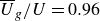 $\overline {U}_{g}/U=0.96$
, further corroborating our claim surrounding the work of Green & Gerrard (Reference Green and Gerrard1993).
$\overline {U}_{g}/U=0.96$
, further corroborating our claim surrounding the work of Green & Gerrard (Reference Green and Gerrard1993).

Figure 5. Temporal evolution of the average streamwise gap velocity
 $U_{g}/U$
, the non-dimensional lift force
$U_{g}/U$
, the non-dimensional lift force
 $C_{l}$
and the front stagnation angle
$C_{l}$
and the front stagnation angle
 $\theta$
, which varies clockwise with
$\theta$
, which varies clockwise with
 $\theta =0$
located at the front of the cylinder on the horizontal centreline. Velocity
$\theta =0$
located at the front of the cylinder on the horizontal centreline. Velocity
 $U_{g}$
is calculated using the velocity profile along the vertical centreline between the top of the cylinder and the liquid–gas interface. In (a),
$U_{g}$
is calculated using the velocity profile along the vertical centreline between the top of the cylinder and the liquid–gas interface. In (a),
 $\overline {U}_{g}$
denotes the temporal mean of
$\overline {U}_{g}$
denotes the temporal mean of
 $U_{g}$
. The Reynolds and Weber numbers are set to
$U_{g}$
. The Reynolds and Weber numbers are set to
 $ {Re}=150$
and
$ {Re}=150$
and
 $ {We}=1000$
. The remaining parameters are indicated in individual plots.
$ {We}=1000$
. The remaining parameters are indicated in individual plots.
Following our discussion on lift force fluctuations, we now discuss the origin of the non-zero mean lift force
 $\overline {C}_{l}$
seen in figure 4(b). In single-phase flows, the incoming fluid halts at the front of the cylinder, creating a stagnation point. Once the system reaches a dynamic steady state through periodic vortex shedding, this stagnation point oscillates slightly. For instance, at
$\overline {C}_{l}$
seen in figure 4(b). In single-phase flows, the incoming fluid halts at the front of the cylinder, creating a stagnation point. Once the system reaches a dynamic steady state through periodic vortex shedding, this stagnation point oscillates slightly. For instance, at
 $ {Re}=150$
, the stagnation point oscillates
$ {Re}=150$
, the stagnation point oscillates
 ${\approx }1.8^{\circ }$
to either side of the horizontal centreline passing through the cylinder. These oscillations are symmetric, and thus, over one vortex shedding cycle, the combined effect of stagnation pressure and low wake pressure results in a net drag force acting along the positive
${\approx }1.8^{\circ }$
to either side of the horizontal centreline passing through the cylinder. These oscillations are symmetric, and thus, over one vortex shedding cycle, the combined effect of stagnation pressure and low wake pressure results in a net drag force acting along the positive
 $x$
direction while
$x$
direction while
 $\overline {C}_{l}\rightarrow 0$
. However, this symmetry breaks down when a liquid–gas interface is introduced. Figures 5(b
$\overline {C}_{l}\rightarrow 0$
. However, this symmetry breaks down when a liquid–gas interface is introduced. Figures 5(b
 $_{1}$
) and 5(b
$_{1}$
) and 5(b
 $_{2}$
) show the evolution of the instantaneous lift force
$_{2}$
) show the evolution of the instantaneous lift force
 ${C}_{l}$
and the stagnation angle
${C}_{l}$
and the stagnation angle
 $\theta$
for
$\theta$
for
 $h/D=1.5$
and
$h/D=1.5$
and
 $1$
at
$1$
at
 $ {Bo}=5000$
. Here, the stagnation point no longer oscillates symmetrically but instead concentrates in the upper left quadrant of the cylinder. Consequently, the vertical component of the force from the stagnation pressure does not vanish over one shedding cycle, contributing to a sustained non-zero mean lift force. Essentially, the displacement of the stagnation point due to the liquid–gas interface introduces bias in the lift force signal, making
$ {Bo}=5000$
. Here, the stagnation point no longer oscillates symmetrically but instead concentrates in the upper left quadrant of the cylinder. Consequently, the vertical component of the force from the stagnation pressure does not vanish over one shedding cycle, contributing to a sustained non-zero mean lift force. Essentially, the displacement of the stagnation point due to the liquid–gas interface introduces bias in the lift force signal, making
 $\overline {C}_{l}$
non-zero. As
$\overline {C}_{l}$
non-zero. As
 $h/D$
decreases, the stagnation point shifts further into the upper left quadrant, moving away from the horizontal centreline, which increases
$h/D$
decreases, the stagnation point shifts further into the upper left quadrant, moving away from the horizontal centreline, which increases
 $\overline {C}_{l}$
even more (see figures 4
b and 5
b
$\overline {C}_{l}$
even more (see figures 4
b and 5
b
 $_{2}$
).
$_{2}$
).
Figure 4(c) shows the variation in the mean lift force
 $\overline {C}_{l}$
for multiple Bond numbers and submergence depths. At
$\overline {C}_{l}$
for multiple Bond numbers and submergence depths. At
 $h/D=2.5$
, the difference in
$h/D=2.5$
, the difference in
 $\overline {C}_{l}$
across various
$\overline {C}_{l}$
across various
 $ {Bo}$
values is marginal. Notably, they all fall within the reduced deformation regime indicated in figure 2. However, as
$ {Bo}$
values is marginal. Notably, they all fall within the reduced deformation regime indicated in figure 2. However, as
 $h/D$
decreases, the
$h/D$
decreases, the
 $\overline {C}_{l}$
values for different Bond numbers start to diverge. This branching occurs within the
$\overline {C}_{l}$
values for different Bond numbers start to diverge. This branching occurs within the
 $h/D$
range marked by the red zone in figure 4(c), and it corresponds to the regime transition as
$h/D$
range marked by the red zone in figure 4(c), and it corresponds to the regime transition as
 $ {Bo}$
varies for a specific
$ {Bo}$
varies for a specific
 $h/D$
(see figure 2). For instance, while switching from
$h/D$
(see figure 2). For instance, while switching from
 $h/D=2.5$
to
$h/D=2.5$
to
 $2.25$
,
$2.25$
,
 $ {Bo}=2000$
transitions from the reduced deformation to the gas entrainment regime, while remaining
$ {Bo}=2000$
transitions from the reduced deformation to the gas entrainment regime, while remaining
 $ {Bo}$
values still exhibit reduced deformation of the interface (see figure 2). This transition at
$ {Bo}$
values still exhibit reduced deformation of the interface (see figure 2). This transition at
 $h/D=2.25$
is reflected in figure 4(c) by the increased
$h/D=2.25$
is reflected in figure 4(c) by the increased
 $\overline {C}_{l}$
for
$\overline {C}_{l}$
for
 $ {Bo}=2000$
compared with other Bond numbers. Similar branching patterns are observed for
$ {Bo}=2000$
compared with other Bond numbers. Similar branching patterns are observed for
 $h/D=1.75$
and
$h/D=1.75$
and
 $1.5$
as
$1.5$
as
 $ {Bo}=3000$
and
$ {Bo}=3000$
and
 $4000$
transition to the gas entrainment state. At
$4000$
transition to the gas entrainment state. At
 $h/D=1.5$
, a significant spread in
$h/D=1.5$
, a significant spread in
 $\overline {C}_{l}$
is visible, with more deformable interfaces (lower Bond numbers) producing higher lift forces. To understand this, we examine the instantaneous interface shapes for
$\overline {C}_{l}$
is visible, with more deformable interfaces (lower Bond numbers) producing higher lift forces. To understand this, we examine the instantaneous interface shapes for
 $ {Bo}=2000$
and
$ {Bo}=2000$
and
 $5000$
in figure 4(c). It is observed that at
$5000$
in figure 4(c). It is observed that at
 $ {Bo}=2000$
, the interface deformation near the back of the cylinder reorients the flow towards the cylinder in the negative
$ {Bo}=2000$
, the interface deformation near the back of the cylinder reorients the flow towards the cylinder in the negative
 $y$
direction, thereby generating a higher downward lift force compared with the weakly deformed interface at
$y$
direction, thereby generating a higher downward lift force compared with the weakly deformed interface at
 $ {Bo}=5000$
. As
$ {Bo}=5000$
. As
 $h/D$
decreases below
$h/D$
decreases below
 $1.5$
, the trend reverses within the blue zone on the left in figure 4(c), where all
$1.5$
, the trend reverses within the blue zone on the left in figure 4(c), where all
 $ {Bo}$
curves start to converge. Note that for
$ {Bo}$
curves start to converge. Note that for
 $h/D\lt 1.5$
, all
$h/D\lt 1.5$
, all
 $ {Bo}$
values in figure 4(c) belong to the gas entrainment state. At
$ {Bo}$
values in figure 4(c) belong to the gas entrainment state. At
 $h/D=1$
, all
$h/D=1$
, all
 $ {Bo}$
points nearly collapse with similar
$ {Bo}$
points nearly collapse with similar
 $\overline {C}_{l}$
values, except for
$\overline {C}_{l}$
values, except for
 $ {Bo}=2000$
, indicating a minimal impact of interface deformability. Overall, the net lift force
$ {Bo}=2000$
, indicating a minimal impact of interface deformability. Overall, the net lift force
 $\overline {C}_{l}$
(approximately) exhibits a quadratic variation with the submergence depth
$\overline {C}_{l}$
(approximately) exhibits a quadratic variation with the submergence depth
 $h/D$
(see the black curve in figure 4
c).
$h/D$
(see the black curve in figure 4
c).
Previously, we noted that at
 $ {Bo}=2000$
, vortex shedding ceases when the liquid–gas interface is lowered to the submergence depth
$ {Bo}=2000$
, vortex shedding ceases when the liquid–gas interface is lowered to the submergence depth
 $h/D=1$
(see figure 3
d
$h/D=1$
(see figure 3
d
 $_{1}$
). This is also evident through the temporal variation of the lift force in figure 4(d), as cyclic fluctuations in
$_{1}$
). This is also evident through the temporal variation of the lift force in figure 4(d), as cyclic fluctuations in
 ${C}_{l}$
disappear, and
${C}_{l}$
disappear, and
 ${C}_{l}$
remains nearly constant over time. However, when
${C}_{l}$
remains nearly constant over time. However, when
 $ {Bo}$
is increased to
$ {Bo}$
is increased to
 $3000$
, cyclic fluctuations in
$3000$
, cyclic fluctuations in
 ${C}_{l}$
reappear, as shown in figure 4(d). This particular combination of
${C}_{l}$
reappear, as shown in figure 4(d). This particular combination of
 $ {Bo}=3000$
and
$ {Bo}=3000$
and
 $h/D=1$
exhibits partial vortex shedding similar to that shown in figure 3(g). Another peculiar characteristic of this case is the variability in the peak-to-peak amplitude of the lift force signal over time (see
$h/D=1$
exhibits partial vortex shedding similar to that shown in figure 3(g). Another peculiar characteristic of this case is the variability in the peak-to-peak amplitude of the lift force signal over time (see
 $ {Bo}=3000$
curve in figure 4
d), hinting at the presence of two distinct time scales in the system. The smaller of the two time scales is related to cyclic fluctuations in the lift force, which stems from the periodic shedding of vortices. The second time scale is linked to relatively gradual temporal changes in the peak-to-peak amplitude of lift force cycles. For the physical interpretation of the second time scale, we look at velocity magnitude contours in figure 6(a
$ {Bo}=3000$
curve in figure 4
d), hinting at the presence of two distinct time scales in the system. The smaller of the two time scales is related to cyclic fluctuations in the lift force, which stems from the periodic shedding of vortices. The second time scale is linked to relatively gradual temporal changes in the peak-to-peak amplitude of lift force cycles. For the physical interpretation of the second time scale, we look at velocity magnitude contours in figure 6(a
 $_{1}$
,a
$_{1}$
,a
 $_{2}$
) corresponding to two different time instances marked by black circles in figure 4(d). As illustrated in figure 6(a
$_{2}$
) corresponding to two different time instances marked by black circles in figure 4(d). As illustrated in figure 6(a
 $_{1}$
), the jet emerging through the gap above the cylinder separates from the liquid–gas interface near the back of the cylinder. On the contrary, at a later time in figure 6(a
$_{1}$
), the jet emerging through the gap above the cylinder separates from the liquid–gas interface near the back of the cylinder. On the contrary, at a later time in figure 6(a
 $_{2}$
), it remains attached to the interface. These temporal changes in the orientation of the jet affect the lift force acting on the cylinder and introduce a new time scale associated with jet oscillations. Such metastable states were initially observed in the experiments by Sheridan, Lin & Rockwell (Reference Sheridan, Lin and Rockwell1995; 1Reference Sheridan, Lin and Rockwell1997), which we introduced earlier in § 1.
$_{2}$
), it remains attached to the interface. These temporal changes in the orientation of the jet affect the lift force acting on the cylinder and introduce a new time scale associated with jet oscillations. Such metastable states were initially observed in the experiments by Sheridan, Lin & Rockwell (Reference Sheridan, Lin and Rockwell1995; 1Reference Sheridan, Lin and Rockwell1997), which we introduced earlier in § 1.

Figure 6. (a
 $_{1}$
,a
$_{1}$
,a
 $_{2}$
) Instantaneous snapshots of velocity magnitude
$_{2}$
) Instantaneous snapshots of velocity magnitude
 $|\boldsymbol {u}|$
within the liquid phase. Intensified colour indicates heightened velocity, with dark red representing the highest velocity within the domain. (b) Discrete Fourier transform of the lift force signal. The simulation parameters are {Re, We, Bo,
$|\boldsymbol {u}|$
within the liquid phase. Intensified colour indicates heightened velocity, with dark red representing the highest velocity within the domain. (b) Discrete Fourier transform of the lift force signal. The simulation parameters are {Re, We, Bo,
 $h/D$
} = {
$h/D$
} = {
 $150, 1000, 3000, 1$
}.
$150, 1000, 3000, 1$
}.
To better quantify the metastable dynamics observed at
 $ {Bo}=3000$
and
$ {Bo}=3000$
and
 $h/d=1$
, we analyse the amplitude–frequency spectrum of the lift force signal using the Fourier transform, as shown in figure 6(b). The spectrum reveals a dominant frequency
$h/d=1$
, we analyse the amplitude–frequency spectrum of the lift force signal using the Fourier transform, as shown in figure 6(b). The spectrum reveals a dominant frequency
 $f_{1}D/U=0.212$
, which is consistent with the frequency range reported for other combinations of
$f_{1}D/U=0.212$
, which is consistent with the frequency range reported for other combinations of
 $ {Bo}$
and
$ {Bo}$
and
 $h/D$
in figure 4(a,b), indicating its connection to the vortex shedding. In the lower-frequency range, there is a notable amplitude peak at
$h/D$
in figure 4(a,b), indicating its connection to the vortex shedding. In the lower-frequency range, there is a notable amplitude peak at
 $f_{2}D/U=0.0254$
, which likely represents the signature of the metastable jet. Earlier, Sheridan et al. (Reference Sheridan, Lin and Rockwell1995) qualitatively estimated
$f_{2}D/U=0.0254$
, which likely represents the signature of the metastable jet. Earlier, Sheridan et al. (Reference Sheridan, Lin and Rockwell1995) qualitatively estimated
 $f_{2}/f_{1}\sim \mathcal {O}{ (10^{-2} )}$
in their experiments at high Reynolds numbers. In contrast, numerical simulations by Reichl et al. (Reference Reichl, Hourigan and Thompson2005) and Colagrossi et al. (Reference Colagrossi, Nikolov, Durante, Marrone and Souto-Iglesias2019), conducted at lower Reynolds numbers and without surface tension, reported
$f_{2}/f_{1}\sim \mathcal {O}{ (10^{-2} )}$
in their experiments at high Reynolds numbers. In contrast, numerical simulations by Reichl et al. (Reference Reichl, Hourigan and Thompson2005) and Colagrossi et al. (Reference Colagrossi, Nikolov, Durante, Marrone and Souto-Iglesias2019), conducted at lower Reynolds numbers and without surface tension, reported
 $f_{2}/f_{1}\sim \mathcal {O}{ (10^{-1} )}$
. Our simulation, which includes surface tension, also yields
$f_{2}/f_{1}\sim \mathcal {O}{ (10^{-1} )}$
. Our simulation, which includes surface tension, also yields
 $f_{2}/f_{1}\sim \mathcal {O}{ (10^{-1} )}$
, aligning with the findings of Reichl et al. (Reference Reichl, Hourigan and Thompson2005) and Colagrossi et al. (Reference Colagrossi, Nikolov, Durante, Marrone and Souto-Iglesias2019). The parameters
$f_{2}/f_{1}\sim \mathcal {O}{ (10^{-1} )}$
, aligning with the findings of Reichl et al. (Reference Reichl, Hourigan and Thompson2005) and Colagrossi et al. (Reference Colagrossi, Nikolov, Durante, Marrone and Souto-Iglesias2019). The parameters
 $ {Re}$
,
$ {Re}$
,
 $ {Fr}$
and
$ {Fr}$
and
 $h/D$
in the present case closely match those in their simulations. To resolve the discrepancy in reported
$h/D$
in the present case closely match those in their simulations. To resolve the discrepancy in reported
 $f_{2}/f_{1}$
values, further work needs to be done in the high-Reynolds-number range, although this is beyond the scope of the present article. We note that although high-Reynolds-number simulations are expensive, experimental set-ups are prone to contamination of the liquid–gas interface, which can dramatically influence the dynamics, as pointed out by Reichl et al. (Reference Reichl, Hourigan and Thompson2005). Recently, Zhao et al. (Reference Zhao, Wang, Zhu, Ping, Bao, Zhou, Cao and Cui2021) performed simulations in the turbulent regime but without considering surface tension.
$f_{2}/f_{1}$
values, further work needs to be done in the high-Reynolds-number range, although this is beyond the scope of the present article. We note that although high-Reynolds-number simulations are expensive, experimental set-ups are prone to contamination of the liquid–gas interface, which can dramatically influence the dynamics, as pointed out by Reichl et al. (Reference Reichl, Hourigan and Thompson2005). Recently, Zhao et al. (Reference Zhao, Wang, Zhu, Ping, Bao, Zhou, Cao and Cui2021) performed simulations in the turbulent regime but without considering surface tension.
3.3.
Interfacial waves at
 $ {Bo}=100$

The remainder of our discussion in this article focuses on specific features of the liquid–gas interface observed in our parameter space. In this subsection, we analyse interfacial waves at a fixed Bond number
 $ {Bo}=100$
for two submergence depths:
$ {Bo}=100$
for two submergence depths:
 $h/D=2.5$
and
$h/D=2.5$
and
 $1.25$
, as marked in figure 2. Apart from the intensity of interfacial disturbances, a notable distinction between these cases is the breakup of the interface, observed only at
$1.25$
, as marked in figure 2. Apart from the intensity of interfacial disturbances, a notable distinction between these cases is the breakup of the interface, observed only at
 $h/D=1.25$
(see snapshots in figure 3).
$h/D=1.25$
(see snapshots in figure 3).
Figure 7 illustrates the colour-coded variation of interface elevation
 $y/D$
in space and time relative to the unperturbed interface height
$y/D$
in space and time relative to the unperturbed interface height
 $h/D$
. Starting at the location
$h/D$
. Starting at the location
 $x/D=0$
above the cylinder, the interface undergoes static deformation with relative elevation
$x/D=0$
above the cylinder, the interface undergoes static deformation with relative elevation
 $(y-h)/D$
approaching the size of the cylinder for both
$(y-h)/D$
approaching the size of the cylinder for both
 $h/D$
values. As we enter the wake region, beginning around
$h/D$
values. As we enter the wake region, beginning around
 $x/D=5$
, the interface deformation becomes time-dependent regardless of
$x/D=5$
, the interface deformation becomes time-dependent regardless of
 $h/D$
when recorded at a given
$h/D$
when recorded at a given
 $x/D$
. However, the temporal deformation pattern varies depending on the value of
$x/D$
. However, the temporal deformation pattern varies depending on the value of
 $h/D$
. For instance, at
$h/D$
. For instance, at
 $x/D=10$
, the interface oscillates on either side of the unperturbed height for
$x/D=10$
, the interface oscillates on either side of the unperturbed height for
 $h/D=1.25$
, whereas for
$h/D=1.25$
, whereas for
 $h/D=2.5$
, it always fluctuates above the unperturbed height. The transition from static to time-varying deformation arises due to the influence of periodically shed Strouhal vortices. Further downstream, both cases exhibit interface oscillations below their original elevation
$h/D=2.5$
, it always fluctuates above the unperturbed height. The transition from static to time-varying deformation arises due to the influence of periodically shed Strouhal vortices. Further downstream, both cases exhibit interface oscillations below their original elevation
 $h/D$
, which is indicated by the extended blue region spanning several diameters in figure 7. As Strouhal vortices weaken, the interface attempts to regain the original elevation. However, the recoil from buoyancy and surface tension leads to an overshoot in elevation before reaching the equilibrium, reminiscent of the damped oscillations of a standing gravity or capillary wave (Prosperetti Reference Prosperetti1981). The overshoot is evident through the red-coloured band between
$h/D$
, which is indicated by the extended blue region spanning several diameters in figure 7. As Strouhal vortices weaken, the interface attempts to regain the original elevation. However, the recoil from buoyancy and surface tension leads to an overshoot in elevation before reaching the equilibrium, reminiscent of the damped oscillations of a standing gravity or capillary wave (Prosperetti Reference Prosperetti1981). The overshoot is evident through the red-coloured band between
 $x/D=35$
and
$x/D=35$
and
 $45$
. At any given time, on a length scale approaching the extent of the vortex street (filtering out small-scale features), we can notice one large-scale interfacial wave represented by two peaks situated near
$45$
. At any given time, on a length scale approaching the extent of the vortex street (filtering out small-scale features), we can notice one large-scale interfacial wave represented by two peaks situated near
 $x/D=0$
and
$x/D=0$
and
 $45$
(red zones in figure 7), and a valley in between (blue zone). This is also visible through snapshots in figure 3. As we refine this coarse-grained description by adopting a length scale comparable to or smaller than the cylinder diameter, small-scale deformation waves become apparent, which ride on the large-scale wave.
$45$
(red zones in figure 7), and a valley in between (blue zone). This is also visible through snapshots in figure 3. As we refine this coarse-grained description by adopting a length scale comparable to or smaller than the cylinder diameter, small-scale deformation waves become apparent, which ride on the large-scale wave.

Figure 7. Spatio-temporal evolution of interfacial perturbations for submergence depths (a)
 $h/D=2.5$
and (b)
$h/D=2.5$
and (b)
 $h/D=1.25$
at a Bond number
$h/D=1.25$
at a Bond number
 $ {Bo}=100$
. These (
$ {Bo}=100$
. These (
 $ {Bo}$
,
$ {Bo}$
,
 $h/D$
) coordinates belong to the interfacial wave regime, where gas entrainment is observed at
$h/D$
) coordinates belong to the interfacial wave regime, where gas entrainment is observed at
 $h/D{=}1.25$
and absent at
$h/D{=}1.25$
and absent at
 $h/D{=}2.5$
(see figure 2). The Reynolds and Weber numbers are fixed at
$h/D{=}2.5$
(see figure 2). The Reynolds and Weber numbers are fixed at
 $ {Re}=150$
and
$ {Re}=150$
and
 $ {We}=1000$
.
$ {We}=1000$
.
Another interesting point to note from figure 7 is the orientation of the emerging pattern. The orientation of various contour levels corresponding to different elevations provides a measure of the phase speed
 $c$
. Based on this, the inverse slope of the yellow line in figure 7(a) yields
$c$
. Based on this, the inverse slope of the yellow line in figure 7(a) yields
 $c=\Delta x/ \Delta t=0.92U$
, indicating a lag between the motion of the bulk liquid and interfacial waves. A similar phase speed is also observed at a lower submergence depth in figure 7(b). However, in the mid-downstream area, high-amplitude deformations with negative relative elevation move at a different phase speed of
$c=\Delta x/ \Delta t=0.92U$
, indicating a lag between the motion of the bulk liquid and interfacial waves. A similar phase speed is also observed at a lower submergence depth in figure 7(b). However, in the mid-downstream area, high-amplitude deformations with negative relative elevation move at a different phase speed of
 $c=0.82U$
, as suggested by the magenta line in figure 7(b). From snapshots in figure 3(a,b), we estimate the wavelength of the deformation pattern to be
$c=0.82U$
, as suggested by the magenta line in figure 7(b). From snapshots in figure 3(a,b), we estimate the wavelength of the deformation pattern to be
 $\lambda \approx 5D$
in both cases.
$\lambda \approx 5D$
in both cases.
Following the linear theory of travelling capillary–gravity waves (Lighthill Reference Lighthill1978), the phase speed
 $c^{r}$
of a capillary–gravity wave relative to still liquid is given by
$c^{r}$
of a capillary–gravity wave relative to still liquid is given by
 \begin{eqnarray} \left (\frac {c^{r}}{U}\right )^{2}{=}\underbrace {\left (\frac {2\pi }{ {We}}\right )\left (\frac {D}{\lambda }\right )}_{\substack { \text {surface-tension-} \\ \text {driven}}}{+}\underbrace {\left (\frac { {Bo}}{2\pi {We}}\right )\left (\frac {\lambda }{D}\right )}_{\substack { \text {gravity-driven}}}, \end{eqnarray}
where
 $\lambda$
denotes the wavelength (note that
$\lambda$
denotes the wavelength (note that
 $ {Bo}/ {We}=1/ {Fr}^{2}$
). Using the phase speed relation (3.2), we derive the minimum phase speed of a realisable capillary–gravity wave relative to still liquid:
$ {Bo}/ {We}=1/ {Fr}^{2}$
). Using the phase speed relation (3.2), we derive the minimum phase speed of a realisable capillary–gravity wave relative to still liquid:
 $c^{r}_{m}/U= (4 {Bo}/ {We}^{2} )^{1/4}$
. Given
$c^{r}_{m}/U= (4 {Bo}/ {We}^{2} )^{1/4}$
. Given
 $ {Bo}=100$
and
$ {Bo}=100$
and
 $ {We}=1000$
, we obtain
$ {We}=1000$
, we obtain
 $c^{r}_{m}=0.14U$
, which is about
$c^{r}_{m}=0.14U$
, which is about
 $1.75$
times the relative phase speed
$1.75$
times the relative phase speed
 $U-c$
shown by the yellow line in figure 7, potentially hinting at a markedly different nature of the present interfacial waves. The relative phase speed associated with the magenta line in figure 7(b) is above the threshold phase speed
$U-c$
shown by the yellow line in figure 7, potentially hinting at a markedly different nature of the present interfacial waves. The relative phase speed associated with the magenta line in figure 7(b) is above the threshold phase speed
 $c^{r}_{m}$
, although it occurs far from the region of wave onset. Note that
$c^{r}_{m}$
, although it occurs far from the region of wave onset. Note that
 $c^{r}$
and
$c^{r}$
and
 $c^{r}_{m}$
are derived under the assumption that the circular cylinder is absent and are valid solely for sinusoidal waveforms.
$c^{r}_{m}$
are derived under the assumption that the circular cylinder is absent and are valid solely for sinusoidal waveforms.
We also compare the observed interfacial waves with the classical Kelvin–Helmholtz (KH) instability, neglecting the effects of gravity and surface tension. According to linear theory, the wave propagation speed for KH instability is
 $c_{\text {KH}}=(\rho _{1}U_{1} +\rho _{2}U_{2})/(\rho _{1}+\rho _{2})$
(Drazin Reference Drazin2002), where the subscripts
$c_{\text {KH}}=(\rho _{1}U_{1} +\rho _{2}U_{2})/(\rho _{1}+\rho _{2})$
(Drazin Reference Drazin2002), where the subscripts
 $1$
and
$1$
and
 $2$
denote the liquid and gas phases, respectively, as shown in figure 1. By substituting
$2$
denote the liquid and gas phases, respectively, as shown in figure 1. By substituting
 $U_{1}=U$
and
$U_{1}=U$
and
 $U_{2}=0$
, we find
$U_{2}=0$
, we find
 $c_{\text {KH}}=0.99U$
, which reasonably approximates the wave speed corresponding to the yellow line in figure 7. It should be noted that
$c_{\text {KH}}=0.99U$
, which reasonably approximates the wave speed corresponding to the yellow line in figure 7. It should be noted that
 $c_{\text {KH}}$
does not account for the influence of the cylinder on KH instability, and the mixing layer in the interfacial region is absent. A refined version of the KH wave speed, referred to as the Dimotakis speed (Dimotakis Reference Dimotakis1986) and commonly used in previous studies (Orazzo, Coppola & de Luca Reference Orazzo, Coppola and de Luca2011; Hoepffner, Blumenthal & Zaleski Reference Hoepffner, Blumenthal and Zaleski2011; Odier et al. Reference Odier, Balarac, Corre and Moureau2015; Ling et al. Reference Ling, Fuster, Zaleski and Tryggvason2017), is expressed as
$c_{\text {KH}}$
does not account for the influence of the cylinder on KH instability, and the mixing layer in the interfacial region is absent. A refined version of the KH wave speed, referred to as the Dimotakis speed (Dimotakis Reference Dimotakis1986) and commonly used in previous studies (Orazzo, Coppola & de Luca Reference Orazzo, Coppola and de Luca2011; Hoepffner, Blumenthal & Zaleski Reference Hoepffner, Blumenthal and Zaleski2011; Odier et al. Reference Odier, Balarac, Corre and Moureau2015; Ling et al. Reference Ling, Fuster, Zaleski and Tryggvason2017), is expressed as
 $c_{\text {Dimotakis}}=(\sqrt {\rho _{1}}U_{1}+\sqrt {\rho _{2}}U_{2})/(\sqrt {\rho _{1}}+\sqrt {\rho _{2}})$
. The estimate
$c_{\text {Dimotakis}}=(\sqrt {\rho _{1}}U_{1}+\sqrt {\rho _{2}}U_{2})/(\sqrt {\rho _{1}}+\sqrt {\rho _{2}})$
. The estimate
 $c_{\text {Dimotakis}}=0.9U$
for the present case aligns well with the range of phase speeds indicated by the yellow and magenta lines in figure 7.
$c_{\text {Dimotakis}}=0.9U$
for the present case aligns well with the range of phase speeds indicated by the yellow and magenta lines in figure 7.
To further our analysis, we investigate the temporal variations in the interface height at the streamwise positions
 $x/D=10$
and
$x/D=10$
and
 $22.5$
. Table 2 reports the dominant frequencies associated with the cyclic fluctuations in interface elevation for submergence depths
$22.5$
. Table 2 reports the dominant frequencies associated with the cyclic fluctuations in interface elevation for submergence depths
 $h/D=2.5$
and
$h/D=2.5$
and
 $1.25$
, which align closely with the vortex shedding frequencies. This correspondence suggests that the the emergence of interfacial waves observed in figure 3(a
$1.25$
, which align closely with the vortex shedding frequencies. This correspondence suggests that the the emergence of interfacial waves observed in figure 3(a
 $_{1}$
,b
$_{1}$
,b
 $_{1}$
) is indeed driven by periodic shedding of Strouhal vortices. Therefore, we refer to these waves as Strouhal waves.
$_{1}$
) is indeed driven by periodic shedding of Strouhal vortices. Therefore, we refer to these waves as Strouhal waves.
Table 2. Dimensionless frequency
 $fD/U$
corresponding to interface oscillations and vortex shedding in the interfacial wave regime at
$fD/U$
corresponding to interface oscillations and vortex shedding in the interfacial wave regime at
 $ {Re}=150$
,
$ {Re}=150$
,
 $ {We}=1000$
and
$ {We}=1000$
and
 $ {Bo}=100$
.
$ {Bo}=100$
.

3.4.
Gas entrainment at
$ {Bo}=1000$

In the present subsection, we focus on the gas entrainment regime observed at
 $ {Bo}=1000$
in figure 2. Before proceeding, we recommend that readers review the brief note in Appendix B on interface breakup and coalescence dynamics in simulations.
$ {Bo}=1000$
in figure 2. Before proceeding, we recommend that readers review the brief note in Appendix B on interface breakup and coalescence dynamics in simulations.
We analyse various statistics related to entrained gas bubbles and liquid droplets formed through bubble collapse, such as their total counts, positions and size distributions. Nevertheless, computing these quantities is not trivial since the liquid–gas interface is captured implicitly with the help of the volume fraction field
 $C$
. To detect bubbles and droplets, existing algorithms in the literature (Herrmann Reference Herrmann2010; Chan et al. Reference Chan, Johnson, Moin and Urzay2021; Gao et al. Reference Gao, Deane, Liu and Shen2021) scan through the domain and first identify a grid point with
$C$
. To detect bubbles and droplets, existing algorithms in the literature (Herrmann Reference Herrmann2010; Chan et al. Reference Chan, Johnson, Moin and Urzay2021; Gao et al. Reference Gao, Deane, Liu and Shen2021) scan through the domain and first identify a grid point with
 $C=0$
(for bubble detection) or
$C=0$
(for bubble detection) or
 $1$
(for droplet detection). They then successively search for neighbouring grid points with the same value of
$1$
(for droplet detection). They then successively search for neighbouring grid points with the same value of
 $C$
until the boundary of the bubble or droplet is detected. This completes the detection of one bubble or droplet. To identify remaining bubbles or droplets, the same two steps are repeated in a loop by excluding grid points belonging to already detected bubbles or droplets.
$C$
until the boundary of the bubble or droplet is detected. This completes the detection of one bubble or droplet. To identify remaining bubbles or droplets, the same two steps are repeated in a loop by excluding grid points belonging to already detected bubbles or droplets.
In our two-dimensional simulations, bubble and droplet statistics are gathered in the post-processing stage using a non-iterative detection algorithm implemented within Matlab
 $^{\circledR }$
. For a given volume fraction field snapshot, Matlab
$^{\circledR }$
. For a given volume fraction field snapshot, Matlab
 $^{\circledR }$
facilitates the extraction of the coordinates tied to isolines of different contour levels. Using this, we are able to obtain the coordinates of
$^{\circledR }$
facilitates the extraction of the coordinates tied to isolines of different contour levels. Using this, we are able to obtain the coordinates of
 $C=0.5$
isolines in the domain, effectively converting our Eulerian interface representation into an equivalent Lagrangian description. In the resulting family of isolines, one of the isolines corresponds to an open curve representing the primary liquid–gas interface, which we eliminate from our subsequent calculations. The remaining isolines are closed curves representing either bubbles or droplets. To bifurcate them into bubbles and droplets, we examine the value of
$C=0.5$
isolines in the domain, effectively converting our Eulerian interface representation into an equivalent Lagrangian description. In the resulting family of isolines, one of the isolines corresponds to an open curve representing the primary liquid–gas interface, which we eliminate from our subsequent calculations. The remaining isolines are closed curves representing either bubbles or droplets. To bifurcate them into bubbles and droplets, we examine the value of
 $C$
at grid cells close to the centroid of each curve. Finally, using the coordinates of individual curves, Matlab
$C$
at grid cells close to the centroid of each curve. Finally, using the coordinates of individual curves, Matlab
 $^{\circledR }$
readily provides the area enclosed by them, from which we derive the diameter
$^{\circledR }$
readily provides the area enclosed by them, from which we derive the diameter
 $d$
of an equivalent circle with the same area, giving us the measure of the size of individual bubbles and droplets. Note that we only focus on the detection of bubbles and droplets; we do not track individual bubbles and droplets as time elapses. Lastly, all the statistics in our subsequent discussion are derived by monitoring bubbles and droplets in a subdomain ranging from
$d$
of an equivalent circle with the same area, giving us the measure of the size of individual bubbles and droplets. Note that we only focus on the detection of bubbles and droplets; we do not track individual bubbles and droplets as time elapses. Lastly, all the statistics in our subsequent discussion are derived by monitoring bubbles and droplets in a subdomain ranging from
 $-D$
to
$-D$
to
 $8D$
in the
$8D$
in the
 $x$
direction and
$x$
direction and
 $-5D$
to
$-5D$
to
 $5D$
in the
$5D$
in the
 $y$
direction.
$y$
direction.
We first examine the number of bubbles and droplets at a given time instance, denoted as
 $\mathcal {N}$
, in the wake region (note that
$\mathcal {N}$
, in the wake region (note that
 $\mathcal {N}$
does not represent the instantaneous count of freshly formed bubbles or droplets). Two such time series are demonstrated in figure 8(a
$\mathcal {N}$
does not represent the instantaneous count of freshly formed bubbles or droplets). Two such time series are demonstrated in figure 8(a
 $_{1}$
,a
$_{1}$
,a
 $_{2}$
) for submergence depths
$_{2}$
) for submergence depths
 $h/D=2.5$
and
$h/D=2.5$
and
 $1$
. A notable spike in bubble count is observed around
$1$
. A notable spike in bubble count is observed around
 $tU/D=25$
and
$tU/D=25$
and
 $30$
for
$30$
for
 $h/D=2.5$
and
$h/D=2.5$
and
 $1$
, respectively. As the flow around the cylinder develops with time, we see oscillations in the instantaneous bubble count for
$1$
, respectively. As the flow around the cylinder develops with time, we see oscillations in the instantaneous bubble count for
 $h/D=2.5$
. On the other hand, the variation of
$h/D=2.5$
. On the other hand, the variation of
 $\mathcal {N}$
with time remains relatively uniform for
$\mathcal {N}$
with time remains relatively uniform for
 $h/D=1$
. These trends can be attributed to corresponding wake states, characterised by periodic and no vortex shedding at
$h/D=1$
. These trends can be attributed to corresponding wake states, characterised by periodic and no vortex shedding at
 $h/D=2.5$
and
$h/D=2.5$
and
 $1$
, respectively. The average bubble count
$1$
, respectively. The average bubble count
 $\overline {\mathcal {N}}$
amplifies by a factor of
$\overline {\mathcal {N}}$
amplifies by a factor of
 ${\approx }4$
when the interface is shifted from
${\approx }4$
when the interface is shifted from
 $h/D=2.5$
to
$h/D=2.5$
to
 $1$
, indicating a substantial rise in gas entrainment. Conversely, the droplet production appears to be only marginally affected by the change in
$1$
, indicating a substantial rise in gas entrainment. Conversely, the droplet production appears to be only marginally affected by the change in
 $h/D$
, as both cases in figure 8(a
$h/D$
, as both cases in figure 8(a
 $_{1}$
,a
$_{1}$
,a
 $_{2}$
) have nearly identical average droplet counts
$_{2}$
) have nearly identical average droplet counts
 $\overline {\mathcal {N}}$
.
$\overline {\mathcal {N}}$
.

Figure 8. (a
 $_{1}$
,a
$_{1}$
,a
 $_{2}$
) Temporal variation of the number of bubbles and droplets
$_{2}$
) Temporal variation of the number of bubbles and droplets
 $\mathcal {N}$
in the wake region. Here
$\mathcal {N}$
in the wake region. Here
 $\overline {\mathcal {N}}$
is the temporal mean of
$\overline {\mathcal {N}}$
is the temporal mean of
 $\mathcal {N}$
. (b
$\mathcal {N}$
. (b
 $_{1}$
,b
$_{1}$
,b
 $_{2}$
) Collection of bubble coordinates recorded over the time interval
$_{2}$
) Collection of bubble coordinates recorded over the time interval
 $20\leqslant tU/D \leqslant 100$
. High-density regions with tightly clustered bubble coordinates are marked in red, whereas those with low bubble density are shown in blue. (c
$20\leqslant tU/D \leqslant 100$
. High-density regions with tightly clustered bubble coordinates are marked in red, whereas those with low bubble density are shown in blue. (c
 $_{1}$
,c
$_{1}$
,c
 $_{2}$
) Multi-scale bubble-size distributions resulting from the gas entrainment phenomenon. The black curves with green shaded areas show bubble-size distributions fitted to the histograms. Here
$_{2}$
) Multi-scale bubble-size distributions resulting from the gas entrainment phenomenon. The black curves with green shaded areas show bubble-size distributions fitted to the histograms. Here
 $\sum \mathcal {N}$
denotes the total bubble count over the time interval
$\sum \mathcal {N}$
denotes the total bubble count over the time interval
 $20\leqslant tU/D\leqslant 100$
, and
$20\leqslant tU/D\leqslant 100$
, and
 $d$
is the equivalent bubble diameter, as explained in the main text. The Reynolds and Weber numbers are fixed at
$d$
is the equivalent bubble diameter, as explained in the main text. The Reynolds and Weber numbers are fixed at
 $ {Re}=150$
and
$ {Re}=150$
and
 $ {We}=1000$
. The remaining parameters are indicated in individual plots.
$ {We}=1000$
. The remaining parameters are indicated in individual plots.
To visualise the gas entrainment process over the time interval
 $20\leqslant tU/D\leqslant 100$
, we plot the bubble coordinates identified by our detection algorithm and colour-code them based on their clustering in the flow domain (see Eilers & Goeman (Reference Eilers and Goeman2004) for details). The red colour implies dense clusters of bubbles, and vice versa for blue. This provides a spatial distribution of bubbles, analogous to a joint probability distribution in physical space, as shown in figure 8(b
$20\leqslant tU/D\leqslant 100$
, we plot the bubble coordinates identified by our detection algorithm and colour-code them based on their clustering in the flow domain (see Eilers & Goeman (Reference Eilers and Goeman2004) for details). The red colour implies dense clusters of bubbles, and vice versa for blue. This provides a spatial distribution of bubbles, analogous to a joint probability distribution in physical space, as shown in figure 8(b
 $_{1}$
,b
$_{1}$
,b
 $_{2}$
) for submergence depths
$_{2}$
) for submergence depths
 $h/D=2.5$
and
$h/D=2.5$
and
 $1$
. Interestingly, one can also notice the travel paths of different bubbles through trajectories emerging from coordinates. At
$1$
. Interestingly, one can also notice the travel paths of different bubbles through trajectories emerging from coordinates. At
 $h/D=2.5$
, bubbles are concentrated in a narrow region near the liquid–gas interface. Most gas bubbles are produced where the coordinates are marked in red and yellow in figure 8(b
$h/D=2.5$
, bubbles are concentrated in a narrow region near the liquid–gas interface. Most gas bubbles are produced where the coordinates are marked in red and yellow in figure 8(b
 $_{1}$
). Some newly produced bubbles travel downstream parallel to the interface, while others rise to the interface due to buoyancy and collapse, which is evident through trajectories terminating near the interface. When the submergence depth is reduced to
$_{1}$
). Some newly produced bubbles travel downstream parallel to the interface, while others rise to the interface due to buoyancy and collapse, which is evident through trajectories terminating near the interface. When the submergence depth is reduced to
 $h/D=1$
, there is a significant spread in bubble distribution in the wake region, spanning about a couple of diameters in the
$h/D=1$
, there is a significant spread in bubble distribution in the wake region, spanning about a couple of diameters in the
 $y$
direction. The area with high bubble density (red-coloured coordinates) expands and shifts its orientation compared to the
$y$
direction. The area with high bubble density (red-coloured coordinates) expands and shifts its orientation compared to the
 $h/D=2.5$
case, suggesting a different nature of the interface breakup process, which will be explored further in our subsequent discussion. The merging of gas bubbles with the free surface (i.e. bursting bubbles) still persists at
$h/D=2.5$
case, suggesting a different nature of the interface breakup process, which will be explored further in our subsequent discussion. The merging of gas bubbles with the free surface (i.e. bursting bubbles) still persists at
 $h/D=1$
, but more bubbles are transported to distant wake regions than at
$h/D=1$
, but more bubbles are transported to distant wake regions than at
 $h/D=2.5$
(mainly during the early stages).
$h/D=2.5$
(mainly during the early stages).
To complete the basic statistical description of the gas entrainment process, we examine the bubble-size distributions shown in figure 8(c
 $_{1}$
,c
$_{1}$
,c
 $_{2}$
) for submergence depths of
$_{2}$
) for submergence depths of
 $h/D=2.5$
and
$h/D=2.5$
and
 $1$
. These distributions are based on bubbles observed over the time interval
$1$
. These distributions are based on bubbles observed over the time interval
 $20\leqslant tU/D\leqslant 100$
. The entrainment of gas bubbles begins at
$20\leqslant tU/D\leqslant 100$
. The entrainment of gas bubbles begins at
 $tU/D\approx 4$
and
$tU/D\approx 4$
and
 ${\approx }14$
for
${\approx }14$
for
 $h/D=1$
and
$h/D=1$
and
 $2.5$
, respectively. In the initial stages of entrainment, large gas bubbles may form, particularly at lower
$2.5$
, respectively. In the initial stages of entrainment, large gas bubbles may form, particularly at lower
 $h/D$
values, resulting in outliers. To circumvent these anomalies, we begin our observations at
$h/D$
values, resulting in outliers. To circumvent these anomalies, we begin our observations at
 $tU/D=20$
for both cases. The size distributions show two preferred bubble sizes for each submergence depth, indicated by two peaks on either side of the equivalent bubble diameter
$tU/D=20$
for both cases. The size distributions show two preferred bubble sizes for each submergence depth, indicated by two peaks on either side of the equivalent bubble diameter
 $d/D= 0.05$
in figure 8(c
$d/D= 0.05$
in figure 8(c
 $_{1}$
,c
$_{1}$
,c
 $_{2}$
). The upper bound of the bubble-size distribution is
$_{2}$
). The upper bound of the bubble-size distribution is
 $d/D=0.3$
, regardless of
$d/D=0.3$
, regardless of
 $h/D$
. While gas entrainment at
$h/D$
. While gas entrainment at
 $h/D=1$
results in a higher bubble count (see figure 8
a
$h/D=1$
results in a higher bubble count (see figure 8
a
 $_{1}$
,a
$_{1}$
,a
 $_{2}$
), entrainment at
$_{2}$
), entrainment at
 $h/D=2.5$
tends to produce larger bubbles (
$h/D=2.5$
tends to produce larger bubbles (
 $d/D\geqslant 0.1$
) more frequently. For bubble sizes below
$d/D\geqslant 0.1$
) more frequently. For bubble sizes below
 $d/D=0.05$
, there is no significant difference in size distributions between
$d/D=0.05$
, there is no significant difference in size distributions between
 $h/D=2.5$
and
$h/D=2.5$
and
 $1$
.
$1$
.
While the multi-scale nature of the bubble-size distributions in figure 8(c
 $_{1}$
,c
$_{1}$
,c
 $_{2}$
) is intriguing, understanding its origin is equally crucial. To explore this, we examine the breakup dynamics of the liquid–gas interface at different submergence depths. Figure 9 shows the formation of the initial interfacial wave at a submergence depth of
$_{2}$
) is intriguing, understanding its origin is equally crucial. To explore this, we examine the breakup dynamics of the liquid–gas interface at different submergence depths. Figure 9 shows the formation of the initial interfacial wave at a submergence depth of
 $h/D=2.5$
. As the flow around the cylinder develops, it draws the interface towards the cylinder and creates a valley, as seen in figure 9(a). Subsequently, this valley shifts in the downstream direction due to the background flow (see figure 9
b), giving rise to a wave crest in figure 9(c–e). When the wave crest reaches a certain height, it bends downward due to gravity (figure 9
f–h) and eventually impacts the liquid–gas interface. Similar features have been observed in previous two- and three-dimensional numerical studies on deep-water waves (Deike, Popinet & Melville Reference Deike, Popinet and Melville2015; Mostert, Popinet & Deike Reference Mostert, Popinet and Deike2022). Interfacial waves similar to that in figure 9 are named plunging waves.
$h/D=2.5$
. As the flow around the cylinder develops, it draws the interface towards the cylinder and creates a valley, as seen in figure 9(a). Subsequently, this valley shifts in the downstream direction due to the background flow (see figure 9
b), giving rise to a wave crest in figure 9(c–e). When the wave crest reaches a certain height, it bends downward due to gravity (figure 9
f–h) and eventually impacts the liquid–gas interface. Similar features have been observed in previous two- and three-dimensional numerical studies on deep-water waves (Deike, Popinet & Melville Reference Deike, Popinet and Melville2015; Mostert, Popinet & Deike Reference Mostert, Popinet and Deike2022). Interfacial waves similar to that in figure 9 are named plunging waves.

Figure 9. Formation of a plunging wave at the onset of gas entrainment. The simulation parameters are {Re, We, Bo,
 $h/D$
} = {
$h/D$
} = {
 $150, 1000, 1000, 2.5$
}. Note that Cartesian coordinates are in units of the cylinder diameter
$150, 1000, 1000, 2.5$
}. Note that Cartesian coordinates are in units of the cylinder diameter
 $D$
.
$D$
.
Figure 10 illustrates the changes in the vertical position of the crest and valley of the plunging wave depicted in figure 9. Just before the wave breaks, its vertical span, from valley to crest, approaches the cylinder’s diameter. Reducing the Bond number to
 $500$
creates relatively tall plunging waves, and vice versa for a lower Weber number of
$500$
creates relatively tall plunging waves, and vice versa for a lower Weber number of
 $700$
. We notice that the formation of similar plunging breakers occurs frequently for the submergence depth of
$700$
. We notice that the formation of similar plunging breakers occurs frequently for the submergence depth of
 $h/D=2.5$
. Figure 11(a
$h/D=2.5$
. Figure 11(a
 $_{1}$
–a
$_{1}$
–a
 $_{4}$
) shows one such sequence of a plunging breaker at a later time, leading to the entrainment of a gas bubble. Typically, bubbles entrained by plunging breakers are larger than
$_{4}$
) shows one such sequence of a plunging breaker at a later time, leading to the entrainment of a gas bubble. Typically, bubbles entrained by plunging breakers are larger than
 $d/D=0.05$
, which explains the presence of larger bubbles in the bubble-size distribution for
$d/D=0.05$
, which explains the presence of larger bubbles in the bubble-size distribution for
 $h/D=2.5$
in figure 8(c
$h/D=2.5$
in figure 8(c
 $_{1}$
). Moreover, bubble coalescence also contributes to the appearance of larger bubbles in the size distribution.
$_{1}$
). Moreover, bubble coalescence also contributes to the appearance of larger bubbles in the size distribution.

Figure 10. Temporal evolution of the interface position
 $y_{\text {int}}$
in the vertical direction at the valley (
$y_{\text {int}}$
in the vertical direction at the valley (
 $\text {min}(y_{\text {int}}-h)$
) and crest (
$\text {min}(y_{\text {int}}-h)$
) and crest (
 $\text {max}(y_{\text {int}}-h)$
) of a plunging wave for different {
$\text {max}(y_{\text {int}}-h)$
) of a plunging wave for different {
 $ {Bo}$
,
$ {Bo}$
,
 $ {We}$
} combinations. The formation of a plunging wave starts with the appearance of the valley, followed by the development of the crest as the interface rises above the initial height
$ {We}$
} combinations. The formation of a plunging wave starts with the appearance of the valley, followed by the development of the crest as the interface rises above the initial height
 $h$
. The inset shows a plunging wave just before the breaking point for
$h$
. The inset shows a plunging wave just before the breaking point for
 $ {Bo}=500$
and
$ {Bo}=500$
and
 $ {We}=1000$
.
$ {We}=1000$
.
In addition to plunging breakers, we also observe surfing breakers, as shown in figure 11(b
 $_{1}$
–b
$_{1}$
–b
 $_{4}$
). Surfing breakers are characterised by a finger-like wavefront gliding along the primary liquid–gas interface with a thin gas layer in between. This gas layer continuously releases air bubbles from its tail due to the movement of the wavefront and bulk liquid, introducing smaller bubbles with sizes
$_{4}$
). Surfing breakers are characterised by a finger-like wavefront gliding along the primary liquid–gas interface with a thin gas layer in between. This gas layer continuously releases air bubbles from its tail due to the movement of the wavefront and bulk liquid, introducing smaller bubbles with sizes
 $d/D\lt 0.05$
in the bubble-size distribution for
$d/D\lt 0.05$
in the bubble-size distribution for
 $h/D=2.5$
. Additionally, the breakup of larger bubbles due to flow disturbances generates more small bubbles, as seen in figure 11(c
$h/D=2.5$
. Additionally, the breakup of larger bubbles due to flow disturbances generates more small bubbles, as seen in figure 11(c
 $_{1}$
–c
$_{1}$
–c
 $_{4}$
). Our findings on various breakup mechanisms and their effects on the bubble-size distribution are qualitatively similar to those reported by Chan et al. (Reference Chan, Mirjalili, Jain, Urzay, Mani and Moin2019) for the production of multi-scale gas bubbles in turbulent breaking waves. Finally, the sequences in figure 11(d
$_{4}$
). Our findings on various breakup mechanisms and their effects on the bubble-size distribution are qualitatively similar to those reported by Chan et al. (Reference Chan, Mirjalili, Jain, Urzay, Mani and Moin2019) for the production of multi-scale gas bubbles in turbulent breaking waves. Finally, the sequences in figure 11(d
 $_{1}$
–d
$_{1}$
–d
 $_{2}$
) show how droplets are formed due to the bubble collapse. The formation of such film droplets is also observed in experiments on bursting bubbles (Lhuissier & Villermaux Reference Lhuissier and Villermaux2012; Shaw & Deike Reference Shaw and Deike2024).
$_{2}$
) show how droplets are formed due to the bubble collapse. The formation of such film droplets is also observed in experiments on bursting bubbles (Lhuissier & Villermaux Reference Lhuissier and Villermaux2012; Shaw & Deike Reference Shaw and Deike2024).

Figure 11. (a1-4
–c1-4
) Various interface breakup mechanisms associated with the production of multi-scale gas bubbles in the gas entrainment regime. (d1-4
) Birth of film droplets via the collapse of an entrained gas bubble. The simulation parameters are {Re, We, Bo,
 $h/D$
} = {
$h/D$
} = {
 $150, 1000, 1000, 2.5$
}.
$150, 1000, 1000, 2.5$
}.
Contrary to
 $h/D=2.5$
, the entrainment of gas bubbles at
$h/D=2.5$
, the entrainment of gas bubbles at
 $h/D=1$
is driven by a different mechanism. As shown in figure 12, there is no vortex shedding at
$h/D=1$
is driven by a different mechanism. As shown in figure 12, there is no vortex shedding at
 $h/D=1$
. Instead, shear layers formed due to the cylinder, although stable, tilt downward in the direction of the jet-like flow coming out of the gap above the cylinder. Subsequently, the flow within the gap drags the interface with it and forms a gas finger shown in figure 12 (also refer to figure 3
d
$h/D=1$
. Instead, shear layers formed due to the cylinder, although stable, tilt downward in the direction of the jet-like flow coming out of the gap above the cylinder. Subsequently, the flow within the gap drags the interface with it and forms a gas finger shown in figure 12 (also refer to figure 3
d
 $_{1}$
,d
$_{1}$
,d
 $_{2}$
with similar dynamics). This gas finger continuously emits bubbles from its end via the interface breakup and creates a train of small bubbles with sizes typically less than
$_{2}$
with similar dynamics). This gas finger continuously emits bubbles from its end via the interface breakup and creates a train of small bubbles with sizes typically less than
 $d/D=0.05$
. The train of newly formed bubbles travels along the path indicated by the brown arrows. During their transport, these bubbles frequently coalesce with other bubbles, forming larger ones. Eventually, fairly large bubbles deviate from their initial path and begin to rise vertically, as indicated by the grey arrows. The life cycle of a bubble ends when it collapses at the free surface. Thus, the bubble-size distribution for
$d/D=0.05$
. The train of newly formed bubbles travels along the path indicated by the brown arrows. During their transport, these bubbles frequently coalesce with other bubbles, forming larger ones. Eventually, fairly large bubbles deviate from their initial path and begin to rise vertically, as indicated by the grey arrows. The life cycle of a bubble ends when it collapses at the free surface. Thus, the bubble-size distribution for
 $h/d=1$
is regulated by the number of coalescence cascades each bubble undergoes. Relatively large bubbles can appear only through coalescence events. On the other hand, some bubbles do not coalesce and remain small. Such small bubbles drift in the background flow. For instance, notice gas bubbles between
$h/d=1$
is regulated by the number of coalescence cascades each bubble undergoes. Relatively large bubbles can appear only through coalescence events. On the other hand, some bubbles do not coalesce and remain small. Such small bubbles drift in the background flow. For instance, notice gas bubbles between
 $x/D=5$
and
$x/D=5$
and
 $7$
in figure 12, which are trapped in the circulation formed by the incoming flow and backflow.
$7$
in figure 12, which are trapped in the circulation formed by the incoming flow and backflow.

Figure 12. Instantaneous snapshot of the primary liquid–gas interface, entrained gas bubbles, film droplets and shear layers (vorticity isolines in red and blue) arising from the cylinder. The inset provides a close-up view of the gas finger. The simulation parameters are indicated in the plot.
We note that Colagrossi et al. (Reference Colagrossi, Nikolov, Durante, Marrone and Souto-Iglesias2019) previously reported the entrainment of gas bubbles at
 $h/D=0.9$
,
$h/D=0.9$
,
 $ {We}=\infty$
,
$ {We}=\infty$
,
 $ {Fr}=0.55$
and
$ {Fr}=0.55$
and
 $ {Re}=180$
. However, their work did not provide detailed bubble statistics or explore the entrainment mechanism, as their main objective was a numerical comparison of various flow solvers. To further our analysis of gas entrainment at
$ {Re}=180$
. However, their work did not provide detailed bubble statistics or explore the entrainment mechanism, as their main objective was a numerical comparison of various flow solvers. To further our analysis of gas entrainment at
 $h/D=1$
, we also explore a three-dimensional case in § 3.6.
$h/D=1$
, we also explore a three-dimensional case in § 3.6.
3.5.
Influence of
$ { We}$
and
$Re$
on gas entrainment


In this subsection, we briefly discuss the effects of the Weber (
 $We$
) and Reynolds (
$We$
) and Reynolds (
 $Re$
) numbers on gas entrainment, specifically within the ranges
$Re$
) numbers on gas entrainment, specifically within the ranges
 $700\leqslant {We}\leqslant 1100$
and
$700\leqslant {We}\leqslant 1100$
and
 $50\leqslant {Re}\leqslant 150$
. In principle, for any fixed value of the Reynolds number, the Weber number can be independently adjusted by modifying the surface tension
$50\leqslant {Re}\leqslant 150$
. In principle, for any fixed value of the Reynolds number, the Weber number can be independently adjusted by modifying the surface tension
 $\sigma$
, for instance, using surfactants. We use the time-averaged bubble count
$\sigma$
, for instance, using surfactants. We use the time-averaged bubble count
 $\overline {\mathcal {N}}$
and size
$\overline {\mathcal {N}}$
and size
 $\overline {d}/D$
as indicators of gas entrainment intensity. At a Bond number of
$\overline {d}/D$
as indicators of gas entrainment intensity. At a Bond number of
 $ {Bo}=1000$
and a submergence depth of
$ {Bo}=1000$
and a submergence depth of
 $h/D=2.5$
, decreasing the Weber number gradually reduces the formation of gas bubbles, with
$h/D=2.5$
, decreasing the Weber number gradually reduces the formation of gas bubbles, with
 $\overline {\mathcal {N}}$
approaching zero (see figure 13
a
$\overline {\mathcal {N}}$
approaching zero (see figure 13
a
 $_{1}$
). Meanwhile, the time-averaged bubble size
$_{1}$
). Meanwhile, the time-averaged bubble size
 $\overline {d}/D$
fluctuates with
$\overline {d}/D$
fluctuates with
 $ {We}$
but remains within the
$ {We}$
but remains within the
 $\pm 10\,\%$
bound when measured relative to any fixed
$\pm 10\,\%$
bound when measured relative to any fixed
 $ {We}$
. This indicates that changes in
$ {We}$
. This indicates that changes in
 $\overline {\mathcal {N}}$
alone provide a qualitative estimate of the entrained gas volume. Additionally, at
$\overline {\mathcal {N}}$
alone provide a qualitative estimate of the entrained gas volume. Additionally, at
 $ {We}=700$
, gas bubble production becomes intermittent, resulting in a cylinder wake devoid of gas bubbles (
$ {We}=700$
, gas bubble production becomes intermittent, resulting in a cylinder wake devoid of gas bubbles (
 $\mathcal {N}=0$
) during specific time intervals. This is evident from the time series in the inset of figure 13(a
$\mathcal {N}=0$
) during specific time intervals. This is evident from the time series in the inset of figure 13(a
 $_{1}$
).
$_{1}$
).

Figure 13. Impact of the Reynolds (
 $Re$
) and Weber (
$Re$
) and Weber (
 $We$
) numbers on the time-averaged bubble count
$We$
) numbers on the time-averaged bubble count
 $\overline {\mathcal {N}}$
and size
$\overline {\mathcal {N}}$
and size
 $\overline {d}/D$
in the gas entrainment regime for submergence depths
$\overline {d}/D$
in the gas entrainment regime for submergence depths
 $h/D=2.5$
and
$h/D=2.5$
and
 $1$
. The Bond number is fixed at
$1$
. The Bond number is fixed at
 $ {Bo}=1000$
. The time averaging is performed over the interval
$ {Bo}=1000$
. The time averaging is performed over the interval
 $20\leqslant tU/D\leqslant 100$
. The black vertical bars indicate
$20\leqslant tU/D\leqslant 100$
. The black vertical bars indicate
 ${\pm }10\,\%$
variations in
${\pm }10\,\%$
variations in
 $\overline {d}/D$
. Insets in (a
1,a
2) and (b
1) show the time series of the number of bubbles
$\overline {d}/D$
. Insets in (a
1,a
2) and (b
1) show the time series of the number of bubbles
 $\mathcal {N}$
in the wake region for
$\mathcal {N}$
in the wake region for
 $ {We}=700$
and
$ {We}=700$
and
 $ {Re}=50$
, respectively. The top inset in (b
$ {Re}=50$
, respectively. The top inset in (b
 $_{2}$
) illustrates an instantaneous snapshot of the primary liquid–gas interface, entrained gas bubbles and shear layers arising from the cylinder at
$_{2}$
) illustrates an instantaneous snapshot of the primary liquid–gas interface, entrained gas bubbles and shear layers arising from the cylinder at
 $ {Re}=50$
. The bottom inset in (b
$ {Re}=50$
. The bottom inset in (b
 $_{2}$
) provides a zoomed-in view of the gas finger shown in the top inset.
$_{2}$
) provides a zoomed-in view of the gas finger shown in the top inset.
When the submergence depth is reduced to
 $h/D=1$
in figure 13(a
$h/D=1$
in figure 13(a
 $_{2}$
), the behaviour of
$_{2}$
), the behaviour of
 $\overline {\mathcal {N}}$
becomes irregular. For instance, increasing
$\overline {\mathcal {N}}$
becomes irregular. For instance, increasing
 $ {We}$
from
$ {We}$
from
 $1000$
to
$1000$
to
 $1100$
causes
$1100$
causes
 $\overline {\mathcal {N}}$
to drop. However, this reduction is compensated by a corresponding increase in
$\overline {\mathcal {N}}$
to drop. However, this reduction is compensated by a corresponding increase in
 $\overline {d}/D$
. Similarly, a slight rise in
$\overline {d}/D$
. Similarly, a slight rise in
 $\overline {\mathcal {N}}$
from
$\overline {\mathcal {N}}$
from
 $ {We}=800$
to
$ {We}=800$
to
 $700$
is balanced by a corresponding reduction in
$700$
is balanced by a corresponding reduction in
 $\overline {d}/D$
. Compared to the
$\overline {d}/D$
. Compared to the
 $h/D=2.5$
case shown in figure 13(a
$h/D=2.5$
case shown in figure 13(a
 $_{1}$
), surface tension is less effective in suppressing the wake bubble count at
$_{1}$
), surface tension is less effective in suppressing the wake bubble count at
 $h/D=1$
. At the same time,
$h/D=1$
. At the same time,
 $\overline {d}/D$
drops by
$\overline {d}/D$
drops by
 ${\approx }28\,\%$
when switching from
${\approx }28\,\%$
when switching from
 $ {We}=1100$
to
$ {We}=1100$
to
 $700$
. We hypothesise that a broader range of Weber numbers may need to be explored in figure 13(a
$700$
. We hypothesise that a broader range of Weber numbers may need to be explored in figure 13(a
 $_{2}$
) to identify a clear trend in the variation of
$_{2}$
) to identify a clear trend in the variation of
 $\overline {\mathcal {N}}$
at
$\overline {\mathcal {N}}$
at
 $h/D=1$
. This is because the influence of flow disturbances on the free surface is already more pronounced for the small gap ratio of
$h/D=1$
. This is because the influence of flow disturbances on the free surface is already more pronounced for the small gap ratio of
 $h/D=1$
compared with the
$h/D=1$
compared with the
 $h/D=2.5$
case shown in figure 13(a
$h/D=2.5$
case shown in figure 13(a
 $_{1}$
). As a result, the effect of change in surface tension on
$_{1}$
). As a result, the effect of change in surface tension on
 $\overline {\mathcal {N}}$
may not be immediately apparent and could lead to a non-monotonic trend with only minor variations in
$\overline {\mathcal {N}}$
may not be immediately apparent and could lead to a non-monotonic trend with only minor variations in
 $\overline {\mathcal {N}}$
. Previously, in figure 8(a
$\overline {\mathcal {N}}$
. Previously, in figure 8(a
 $_{2}$
) for
$_{2}$
) for
 $ {We}=1000$
, we noted a spike in the bubble count
$ {We}=1000$
, we noted a spike in the bubble count
 $\mathcal {N}$
at the start of gas entrainment. Conversely, at
$\mathcal {N}$
at the start of gas entrainment. Conversely, at
 $ {We}=700$
, surface tension stabilises the onset of gas entrainment, leading to a smoother start without any notable spike, as indicated by the time series in the inset of figure 13(a
$ {We}=700$
, surface tension stabilises the onset of gas entrainment, leading to a smoother start without any notable spike, as indicated by the time series in the inset of figure 13(a
 $_{2}$
).
$_{2}$
).
Figure 13(b
 $_{1}$
) illustrates the effect
$_{1}$
) illustrates the effect
 $ {Re}$
on gas entrainment with parameters {We, Bo,
$ {Re}$
on gas entrainment with parameters {We, Bo,
 $h/D$
} = {
$h/D$
} = {
 $1000, 1000, 2.5$
}. The time-averaged bubble count
$1000, 1000, 2.5$
}. The time-averaged bubble count
 $\overline {\mathcal {N}}$
and size
$\overline {\mathcal {N}}$
and size
 $\overline {d}/D$
show marginal variation in the range
$\overline {d}/D$
show marginal variation in the range
 $100\leqslant {Re}\leqslant 150$
but drops sharply for
$100\leqslant {Re}\leqslant 150$
but drops sharply for
 $ {Re}\lt 100$
. At the lowest
$ {Re}\lt 100$
. At the lowest
 $ {Re}$
of
$ {Re}$
of
 $50$
, several changes in dynamics are observed. First, the entrainment of gas bubbles occurs in a sporadic fashion, as shown in the inset of figure 13(b
$50$
, several changes in dynamics are observed. First, the entrainment of gas bubbles occurs in a sporadic fashion, as shown in the inset of figure 13(b
 $_{1}$
). Second, an instantaneous snapshot of the wake structure in figure 14 reveals the absence of vortex shedding. Third and most importantly, we see the emergence of an interfacial wave in the wake region (see figure 14), differing from the localised deformation seen at higher Reynolds numbers (e.g. see figure 3
c
$_{1}$
). Second, an instantaneous snapshot of the wake structure in figure 14 reveals the absence of vortex shedding. Third and most importantly, we see the emergence of an interfacial wave in the wake region (see figure 14), differing from the localised deformation seen at higher Reynolds numbers (e.g. see figure 3
c
 $_{1}$
). This wave pattern at
$_{1}$
). This wave pattern at
 $ {Re}=50$
is static relative to the background flow, but the wave crest near
$ {Re}=50$
is static relative to the background flow, but the wave crest near
 $x/D=5$
in figure 14 is unstable and undergoes occasional small-scale wave breaking, entraining gas bubbles for short intervals (see inset in figure 13
b
$x/D=5$
in figure 14 is unstable and undergoes occasional small-scale wave breaking, entraining gas bubbles for short intervals (see inset in figure 13
b
 $_{1}$
).
$_{1}$
).

Figure 14. Instantaneous snapshot of the liquid–gas interface and the vorticity field at
 $tU/D=200$
for {Re, We, Bo,
$tU/D=200$
for {Re, We, Bo,
 $h/D$
} = {
$h/D$
} = {
 $50, 1000, 1000, 2.5$
}. Note that Cartesian coordinates are in units of the cylinder diameter
$50, 1000, 1000, 2.5$
}. Note that Cartesian coordinates are in units of the cylinder diameter
 $D$
.
$D$
.
To characterise the interfacial wave in figure 14, we again use Lighthill’s linear theory of travelling capillary–gravity waves (Lighthill Reference Lighthill1978) as a reference (equation (3.2)). Given
 $ {We}= {Bo}=1000$
, the influence of the surface-tension-driven component in (3.2) is negligible. Substituting
$ {We}= {Bo}=1000$
, the influence of the surface-tension-driven component in (3.2) is negligible. Substituting
 $c^{r}={-}U$
in (3.2) results in a gravity wave characterised by
$c^{r}={-}U$
in (3.2) results in a gravity wave characterised by
 $\lambda /D=2\pi$
, which aligns with the spacing between the initial two wave crests in figure 14. Moving further from the cylinder, the distance between consecutive wave crests decreases by about
$\lambda /D=2\pi$
, which aligns with the spacing between the initial two wave crests in figure 14. Moving further from the cylinder, the distance between consecutive wave crests decreases by about
 $0.5D$
. Similar to our findings, Sheridan et al. (Reference Sheridan, Lin and Rockwell1995; Reference Sheridan, Lin and Rockwell1997) also reported the excitation of stationary interfacial waves caused by the presence of the cylinder in their experiments.
$0.5D$
. Similar to our findings, Sheridan et al. (Reference Sheridan, Lin and Rockwell1995; Reference Sheridan, Lin and Rockwell1997) also reported the excitation of stationary interfacial waves caused by the presence of the cylinder in their experiments.
Finally, in figure 13(b
 $_{2}$
), we examine a submergence depth of
$_{2}$
), we examine a submergence depth of
 $h/D=1$
. The time-averaged bubble sizes
$h/D=1$
. The time-averaged bubble sizes
 $\overline {d}/D$
are in the similar range as previous combinations of {
$\overline {d}/D$
are in the similar range as previous combinations of {
 $ {Re}$
,
$ {Re}$
,
 $ {We}$
,
$ {We}$
,
 $h/D$
}. For
$h/D$
}. For
 $100\leqslant {Re}\leqslant 150$
, the time-averaged bubble count
$100\leqslant {Re}\leqslant 150$
, the time-averaged bubble count
 $\overline {\mathcal {N}}$
almost reaches a plateau. Interestingly, for
$\overline {\mathcal {N}}$
almost reaches a plateau. Interestingly, for
 $ {Re}\lt 100$
, we observe the amplification in
$ {Re}\lt 100$
, we observe the amplification in
 $\overline {\mathcal {N}}$
, in contrast to
$\overline {\mathcal {N}}$
, in contrast to
 $h/D=2.5$
in figure 13(b
$h/D=2.5$
in figure 13(b
 $_{1}$
). To understand this, we recall our discussion on the mechanism responsible for the entrainment of gas bubbles at
$_{1}$
). To understand this, we recall our discussion on the mechanism responsible for the entrainment of gas bubbles at
 $h/D=1$
, where it was noted that the production of gas bubbles is driven by the breakup of the gas finger (see figure 12). Lowering the Reynolds number increases the thickness of vorticity layers on the cylinder surface, promoting the formation of a very long gas finger due to shear flow in the gap, as shown in the insets of figure 13(b
$h/D=1$
, where it was noted that the production of gas bubbles is driven by the breakup of the gas finger (see figure 12). Lowering the Reynolds number increases the thickness of vorticity layers on the cylinder surface, promoting the formation of a very long gas finger due to shear flow in the gap, as shown in the insets of figure 13(b
 $_{2}$
) for
$_{2}$
) for
 $ {Re}=50$
. In this case, the gas finger is as long as the cylinder diameter
$ {Re}=50$
. In this case, the gas finger is as long as the cylinder diameter
 $D$
. Also, compare the relative sizes of gas fingers and vorticity layers close to the cylinder at
$D$
. Also, compare the relative sizes of gas fingers and vorticity layers close to the cylinder at
 $ {Re}=50$
in figure 13(b
$ {Re}=50$
in figure 13(b
 $_{2}$
) and at
$_{2}$
) and at
 $ {Re}=150$
in figure 12. The tail of the longer gas finger at
$ {Re}=150$
in figure 12. The tail of the longer gas finger at
 $ {Re}=50$
is more unstable than the shorter finger at
$ {Re}=50$
is more unstable than the shorter finger at
 $ {Re}=150$
, leading to more frequent interface breakups. Consequently, this results in more gas bubbles being entrained over time at lower Reynolds numbers.
$ {Re}=150$
, leading to more frequent interface breakups. Consequently, this results in more gas bubbles being entrained over time at lower Reynolds numbers.
3.6. Gas entrainment in a three-dimensional flow set-up
In this final subsection, we provide an outlook on bubble production through gas entrainment in a three-dimensional configuration. For the range of Reynolds numbers investigated in this study, the occurrence of three-dimensional flow structures is unlikely (Barkley & Henderson Reference Barkley and Henderson1996; Williamson Reference Williamson1996). However, the role of dimensionality in interfacial phenomena involving topological changes, such as breakup events, cannot be determined a priori. If dimensional effects prevail to a greater extent, they may substantially influence the trends associated with various statistical properties of the entrained gas bubbles. Thus, to build further on our two-dimensional findings in the last two subsections, we demonstrate a three-dimensional case with parameters
 $ {Re}=150$
,
$ {Re}=150$
,
 $ {We}=1000$
,
$ {We}=1000$
,
 $ {Bo}=1000$
and
$ {Bo}=1000$
and
 $h/d=1$
. This particular parameter combination represents one of the extreme scenarios since it produces a relatively large quantity of gas bubbles through entrainment, as seen in figures 8 and 13. Notably, for
$h/d=1$
. This particular parameter combination represents one of the extreme scenarios since it produces a relatively large quantity of gas bubbles through entrainment, as seen in figures 8 and 13. Notably, for
 $h/D=2.5$
, entrained gas bubbles penetrate to a shallower depth in the liquid phase compared with
$h/D=2.5$
, entrained gas bubbles penetrate to a shallower depth in the liquid phase compared with
 $h/D=1$
and instead merge with the free surface relatively quickly (see figure 8
b
$h/D=1$
and instead merge with the free surface relatively quickly (see figure 8
b
 $_{1}$
,b
$_{1}$
,b
 $_{2}$
). Consequently, the impact of dimensionality on gas entrainment is expected to be short-lived for
$_{2}$
). Consequently, the impact of dimensionality on gas entrainment is expected to be short-lived for
 $h/D=2.5$
.
$h/D=2.5$
.
The current version of Basilisk (Reference Popinet2013–2024) does not support the use of the cut-cell module (see § 2) for three-dimensional multi-processor simulations involving immersed boundaries. Thus, we utilise the Computational Air-Sea Tank (CAS-Tank) solver, developed by Yang, Lu & Wang (Reference Yang, Lu and Wang2021), to simulate three-dimensional liquid–gas flow. Similar to the Basilisk library, CAS-Tank employs the VOF method for capturing the liquid–gas interface. Additionally, CAS-Tank incorporates the level-set function to compute geometrical parameters such as interface normal and curvature. The coupling between VOF and level set is achieved using the methodology proposed by Sussman & Puckett (Reference Sussman and Puckett2000). Moreover, the numerical stability of CAS-Tank is enhanced by implementing the mass–momentum consistent scheme introduced by Nangia et al. (Reference Nangia, Griffith, Patankar and Bhalla2019). For those interested in recent studies on free-surface flows using CAS-Tank, we refer the reader to Li, Yang & Zhang (Reference Li, Yang and Zhang2024) and Lu et al. (Reference Lu, Yang, He and Shen2024). Finally, the no-slip boundary condition at the curved liquid–cylinder boundary is enforced using the level-set-based sharp interface representation of the solid cylinder. See Cui et al. (Reference Cui, Yang, Jiang, Huang and Shen2017) for further details.
The size of the computational domain is set to
 $45D$
,
$45D$
,
 $30D$
and
$30D$
and
 $3D$
in the
$3D$
in the
 $x$
(streamwise),
$x$
(streamwise),
 $y$
(transverse) and
$y$
(transverse) and
 $z$
(spanwise) directions, respectively. The current domain size in the
$z$
(spanwise) directions, respectively. The current domain size in the
 $x$
and
$x$
and
 $y$
directions yields the same lift force as the previously used larger domain of
$y$
directions yields the same lift force as the previously used larger domain of
 $80D\times 80D$
in two-dimensional simulations. From figure 12, it is evident that interface breakup and bubble formation occur near the cylinder, while the downstream liquid–gas interface further from the cylinder remains undisturbed. Furthermore, no vortex shedding is observed for the current parameters. Based on these observations from a previous two-dimensional simulation, we employ a combination of uniform and non-uniform Cartesian grids in our three-dimensional simulation. A refined uniform grid with a resolution of
$80D\times 80D$
in two-dimensional simulations. From figure 12, it is evident that interface breakup and bubble formation occur near the cylinder, while the downstream liquid–gas interface further from the cylinder remains undisturbed. Furthermore, no vortex shedding is observed for the current parameters. Based on these observations from a previous two-dimensional simulation, we employ a combination of uniform and non-uniform Cartesian grids in our three-dimensional simulation. A refined uniform grid with a resolution of
 $0.025D$
(
$0.025D$
(
 $40$
grid cells per
$40$
grid cells per
 $D$
) is applied within the subdomain extending in the ranges
$D$
) is applied within the subdomain extending in the ranges
 $-1.5\leqslant x/D\leqslant 8.5$
,
$-1.5\leqslant x/D\leqslant 8.5$
,
 $-3\leqslant y/D\leqslant 3$
and
$-3\leqslant y/D\leqslant 3$
and
 $-1.5\leqslant z/D\leqslant 1.5$
(the origin is positioned at the cylinder’s centre). Beyond this subdomain, the grid gradually coarsens towards the domain boundaries, reaching a maximum grid size of
$-1.5\leqslant z/D\leqslant 1.5$
(the origin is positioned at the cylinder’s centre). Beyond this subdomain, the grid gradually coarsens towards the domain boundaries, reaching a maximum grid size of
 $0.18D$
at the edges. Using a two-dimensional simulation, it has been verified that further refining the uniform mesh resolution to
$0.18D$
at the edges. Using a two-dimensional simulation, it has been verified that further refining the uniform mesh resolution to
 $0.0166D$
(
$0.0166D$
(
 $60$
grid cells per
$60$
grid cells per
 $D$
) does not alter the breakup dynamics or the lift force. Lastly, a periodic boundary condition is applied in the spanwise direction, while the boundary conditions in the remaining directions are consistent with those used in the two-dimensional set-up.
$D$
) does not alter the breakup dynamics or the lift force. Lastly, a periodic boundary condition is applied in the spanwise direction, while the boundary conditions in the remaining directions are consistent with those used in the two-dimensional set-up.
Resolving three-dimensional flow and interface features at a moderate resolution within a small subdomain around the cylinder already leads to a substantial number of grid cells (
 $55.728\times 10^{6}$
grid cells in the present case), demanding considerable computational resources. Unlike prior two-dimensional simulations, conducting an extensive parametric study in a three-dimensional set-up is not a viable option. Therefore, as an extension of our two-dimensional observations, we present only one model case where the system’s three-dimensional nature is crucial to interface dynamics.
$55.728\times 10^{6}$
grid cells in the present case), demanding considerable computational resources. Unlike prior two-dimensional simulations, conducting an extensive parametric study in a three-dimensional set-up is not a viable option. Therefore, as an extension of our two-dimensional observations, we present only one model case where the system’s three-dimensional nature is crucial to interface dynamics.
Figure 15(a) provides an instantaneous snapshot of the vorticity field along with gas bubbles in the wake of the cylinder. Similar to the two-dimensional case shown in figure 12, one can observe tilted vorticity layers emerging from the cylinder’s surface. The vorticity layer formed due to the flow separation at the deformed liquid–gas interface is also visible in figure 15(a). This interfacial vorticity enters the wake region and spreads horizontally, forming what can be described as a vorticity carpet. Additionally, the interfacial vorticity plays a role in the cross-annihilation of the vorticity layer at the top of the cylinder and prevents vortex shedding, which is identical to our observation in figure 3(d
 $_{1}$
). Although a similar vorticity annihilation mechanism is also present in figure 12, we have not shown the interfacial vorticity there to maintain a clear visualisation of gas bubbles. The qualitative similarities in flow structures between two- and three-dimensional set-ups are further substantiated by the lift coefficient
$_{1}$
). Although a similar vorticity annihilation mechanism is also present in figure 12, we have not shown the interfacial vorticity there to maintain a clear visualisation of gas bubbles. The qualitative similarities in flow structures between two- and three-dimensional set-ups are further substantiated by the lift coefficient
 $C_{l}$
with values of
$C_{l}$
with values of
 ${-}0.355$
and
${-}0.355$
and
 ${-}0.3452$
for the two- and three-dimensional cases, respectively.
${-}0.3452$
for the two- and three-dimensional cases, respectively.

Figure 15. (a) Volume rendering of the vorticity field surrounding the cylinder and entrained gas bubbles in a three-dimensional flow setting. (b) Production of EGRs by interface breakup and the subsequent fragmentation of EGRs into bubbles in the wake region. The simulation parameters are {Re, We, Bo,
 $h/D$
} = {
$h/D$
} = {
 $150, 1000, 1000, 1$
}.
$150, 1000, 1000, 1$
}.
In a three-dimensional set-up, liquid flow in the gap above the cylinder generates a gas finger (see figure 15), similar to the two-dimensional result shown in figure 12. However, three-dimensional effects become apparent during the entrainment process. The breakup of the gas finger in figure 15(b
 $_{1}$
,b
$_{1}$
,b
 $_{2}$
) leads to the formation of cylindrical gas rolls (labelled as entrained gas roll(EGR)), unlike the planar bubbles observed in figure 12. The successive breakup of the gas finger creates a train of EGRs, analogous to the train of planar bubbles seen in figure 12. These EGRs subsequently undergo fragmentation due to background flow disturbances. A partially fragmented gas roll, EGR1, is highlighted in figure 15(b
$_{2}$
) leads to the formation of cylindrical gas rolls (labelled as entrained gas roll(EGR)), unlike the planar bubbles observed in figure 12. The successive breakup of the gas finger creates a train of EGRs, analogous to the train of planar bubbles seen in figure 12. These EGRs subsequently undergo fragmentation due to background flow disturbances. A partially fragmented gas roll, EGR1, is highlighted in figure 15(b
 $_{1}$
). Later, in figure 15(b
$_{1}$
). Later, in figure 15(b
 $_{2}$
), EGR1 undergoes complete fragmentation, leaving no remnants. Simultaneously, the fragmentation of the next gas roll in the sequence begins, as indicated by the partially fragmented EGR2 in figure 15(b
$_{2}$
), EGR1 undergoes complete fragmentation, leaving no remnants. Simultaneously, the fragmentation of the next gas roll in the sequence begins, as indicated by the partially fragmented EGR2 in figure 15(b
 $_{2}$
). The ongoing fragmentation of EGRs results in a swarm of rising bubbles in the wake region. Thus, it is clear that the breakup mechanisms differ significantly between two- and three-dimensional flows.
$_{2}$
). The ongoing fragmentation of EGRs results in a swarm of rising bubbles in the wake region. Thus, it is clear that the breakup mechanisms differ significantly between two- and three-dimensional flows.
We also collect bubble statistics using the detection algorithm developed by Herrmann (Reference Herrmann2010). A brief discussion on the implementation of the bubble detection method within the CAS-Tank solver can be found in Appendix C. Figure 16 shows the distribution of entrained rolls and bubbles in the wake. Unlike the two-dimensional result shown in figure 8(b
 $_{2}$
), the high-concentration regions in figure 16(a
$_{2}$
), the high-concentration regions in figure 16(a
 $_{1}$
) are positioned away from the location where the gas finger breaks. This shift is due to the fragmentation of EGRs into multiple bubbles, which occurs a few diameters away from the gas finger. The spread of entrained bubbles in the
$_{1}$
) are positioned away from the location where the gas finger breaks. This shift is due to the fragmentation of EGRs into multiple bubbles, which occurs a few diameters away from the gas finger. The spread of entrained bubbles in the
 $y$
direction in figure 16(a
$y$
direction in figure 16(a
 $_{1}$
), which is about twice the cylinder diameter, remains consistent with the two-dimensional case shown in figure 8(b
$_{1}$
), which is about twice the cylinder diameter, remains consistent with the two-dimensional case shown in figure 8(b
 $_{2}$
). Observing the bubble distribution from above in figure 16(a
$_{2}$
). Observing the bubble distribution from above in figure 16(a
 $_{2}$
) reveals a spanwise wave-like periodic pattern of high-concentration regions with a wavelength of
$_{2}$
) reveals a spanwise wave-like periodic pattern of high-concentration regions with a wavelength of
 ${\approx }D$
. The wavelength of this pattern is linked to how the perturbations at the interface of EGRs develop and the subsequent breakup process. However, further investigation is needed to verify whether the spanwise domain size affects the wavelength. The time-averaged bubble count in the present three-dimensional case is
${\approx }D$
. The wavelength of this pattern is linked to how the perturbations at the interface of EGRs develop and the subsequent breakup process. However, further investigation is needed to verify whether the spanwise domain size affects the wavelength. The time-averaged bubble count in the present three-dimensional case is
 $\mathcal {\overline {N}}=536.07$
, which is higher than the two-dimensional bubble count in figure 8(a
$\mathcal {\overline {N}}=536.07$
, which is higher than the two-dimensional bubble count in figure 8(a
 $_{2}$
), as expected. The mean bubble sizes are
$_{2}$
), as expected. The mean bubble sizes are
 $\overline {d}/D=0.05$
and
$\overline {d}/D=0.05$
and
 $0.059$
for the two- and three-dimensional cases, which are still of the same order. However, gas entrainment in the three-dimensional system yields bubbles with a mean size
$0.059$
for the two- and three-dimensional cases, which are still of the same order. However, gas entrainment in the three-dimensional system yields bubbles with a mean size
 $18{\,\%}$
larger than that of the two-dimensional counterpart.
$18{\,\%}$
larger than that of the two-dimensional counterpart.

Figure 16. Projection of bubble coordinates onto the (a
 $_{1}$
)
$_{1}$
)
 $xy$
and (a
$xy$
and (a
 $_{2}$
)
$_{2}$
)
 $xz$
planes in a three-dimensional gas entrainment process. Both projections include a collection of bubble coordinates recorded over the time window
$xz$
planes in a three-dimensional gas entrainment process. Both projections include a collection of bubble coordinates recorded over the time window
 ${\Delta }tU/D=80$
. High-density regions with tightly clustered bubble coordinates are marked in red, whereas those with low bubble density are shown in blue. (b
${\Delta }tU/D=80$
. High-density regions with tightly clustered bubble coordinates are marked in red, whereas those with low bubble density are shown in blue. (b
 $_{1}$
,b
$_{1}$
,b
 $_{2}$
) Bubble-size (
$_{2}$
) Bubble-size (
 $d/D$
) distributions resulting from the gas entrainment phenomenon. Here
$d/D$
) distributions resulting from the gas entrainment phenomenon. Here
 $\mathcal {N}$
,
$\mathcal {N}$
,
 $\mathcal {P}(d)$
and
$\mathcal {P}(d)$
and
 $a_{N}$
denote the number of bubbles, time-averaged bubble-size density and size of the finest computational cell, respectively. The black curve with green shaded area in (b
$a_{N}$
denote the number of bubbles, time-averaged bubble-size density and size of the finest computational cell, respectively. The black curve with green shaded area in (b
 $_{1}$
) shows the bubble-size distribution fitted to the histograms. The simulation parameters are {Re, We, Bo,
$_{1}$
) shows the bubble-size distribution fitted to the histograms. The simulation parameters are {Re, We, Bo,
 $h/D$
} = {
$h/D$
} = {
 $150, 1000, 1000, 1$
}.
$150, 1000, 1000, 1$
}.
The consequences of distinction in the breakup mechanisms between two- and three-dimensional cases become apparent upon examining corresponding bubble-size distributions shown in figures8(c
 $_{2}$
) and 16(b
$_{2}$
) and 16(b
 $_{1}$
). The two-dimensional size distribution (figure 8
c
$_{1}$
). The two-dimensional size distribution (figure 8
c
 $_{2}$
) loses its bimodal nature in a three-dimensional setting (figure 16
b
$_{2}$
) loses its bimodal nature in a three-dimensional setting (figure 16
b
 $_{1}$
). In three dimensions, most bubbles do not form directly from the free surface; instead, they result from the breakup of EGRs. Additionally, bubbles in the wake region are more densely packed in three dimensions due to a significantly higher bubble count. This increased density can dampen the subsequent fragmentation of bubbles caused by background flow disturbances, leading to larger bubbles and a modified size distribution compared with the two-dimensional entrainment case.
$_{1}$
). In three dimensions, most bubbles do not form directly from the free surface; instead, they result from the breakup of EGRs. Additionally, bubbles in the wake region are more densely packed in three dimensions due to a significantly higher bubble count. This increased density can dampen the subsequent fragmentation of bubbles caused by background flow disturbances, leading to larger bubbles and a modified size distribution compared with the two-dimensional entrainment case.
Building on existing studies of bubble entrainment and multi-phase turbulent flows (Deane & Stokes Reference Deane and Stokes2002; Hendrickson et al. Reference Hendrickson, Weymouth, Yu and Yue2019; Mostert et al. Reference Mostert, Popinet and Deike2022; Di Giorgio, Pirozzoli & Iafrati Reference Di Giorgio, Pirozzoli and Iafrati2022; Roccon, Zonta & Soldati Reference Roccon, Zonta and Soldati2023; Li et al. Reference Li, Yang and Zhang2024), we investigate how the time-averaged bubble-size density
 \begin{eqnarray} \mathcal {P}(d){=}\displaystyle {\frac {1}{(80D/U)}}\left (\int \limits ^{t{+}80D/U}_{t}\displaystyle {\frac {\mathcal {N}(d,t;b)}{Vb}{\textrm d}t}\right ) \end{eqnarray}
varies with the diameter
 $d/D$
of the entrained bubbles. Using a bin radius of
$d/D$
of the entrained bubbles. Using a bin radius of
 $b=0.005D$
in (3.3), we compute
$b=0.005D$
in (3.3), we compute
 $\mathcal {P}(d)$
by gathering statistics within a fluid volume
$\mathcal {P}(d)$
by gathering statistics within a fluid volume
 $V$
, defined as a cuboid extending in the ranges
$V$
, defined as a cuboid extending in the ranges
 $0\leqslant x\leqslant 8D$
,
$0\leqslant x\leqslant 8D$
,
 $-3D\leqslant y\leqslant h$
and
$-3D\leqslant y\leqslant h$
and
 $-1.5D\leqslant z\leqslant 1.5D$
.
$-1.5D\leqslant z\leqslant 1.5D$
.
Figure 16(b
 $_{2}$
) presents the time-averaged bubble-size density,
$_{2}$
) presents the time-averaged bubble-size density,
 $\mathcal {P}(d)$
, for bubble sizes
$\mathcal {P}(d)$
, for bubble sizes
 $d/D$
exceeding the size of the finest grid cell,
$d/D$
exceeding the size of the finest grid cell,
 $a_{N}$
. Previous studies across various turbulent flow scenarios have established that
$a_{N}$
. Previous studies across various turbulent flow scenarios have established that
 $\mathcal {P}(d)$
typically follows a
$\mathcal {P}(d)$
typically follows a
 ${-}10/3$
power law (Dean & Stokes Reference Deane and Stokes2002; Roccon et al. Reference Roccon, Zonta and Soldati2023; Li et al. Reference Li, Yang and Zhang2024). However, in the current case with unsteady laminar flow and ongoing air entertainment,
${-}10/3$
power law (Dean & Stokes Reference Deane and Stokes2002; Roccon et al. Reference Roccon, Zonta and Soldati2023; Li et al. Reference Li, Yang and Zhang2024). However, in the current case with unsteady laminar flow and ongoing air entertainment,
 $\mathcal {P}(d)$
declines more rapidly with increasing
$\mathcal {P}(d)$
declines more rapidly with increasing
 $d/D$
, as indicated by the
$d/D$
, as indicated by the
 ${-}9/2$
power law in figure 16(b
${-}9/2$
power law in figure 16(b
 $_{2}$
). Such a deviation from the
$_{2}$
). Such a deviation from the
 ${-}10/3$
power law is not unprecedented and was recently observed by Hendrickson et al. (Reference Hendrickson, Weymouth, Yu and Yue2019) in their large-eddy simulation study of the canonical stern geometry. A comprehensive investigation into the scaling behaviour of
${-}10/3$
power law is not unprecedented and was recently observed by Hendrickson et al. (Reference Hendrickson, Weymouth, Yu and Yue2019) in their large-eddy simulation study of the canonical stern geometry. A comprehensive investigation into the scaling behaviour of
 $\mathcal {P}(d)$
for different combinations of dimensionless parameters in the current set-up is planned for future work.
$\mathcal {P}(d)$
for different combinations of dimensionless parameters in the current set-up is planned for future work.
4. Summary and concluding remarks
We presented a tFSI study involving liquid–gas flow across a stationary circular cylinder, extending the classical single-phase flow set-up. Our work builds on previous numerical investigations of a similar flow configuration by incorporating a liquid–gas interface that has finite surface tension and varies in deformability across a broad range of Bond (
 $Bo$
) numbers. We placed particular emphasis on classifying the emergent interface dynamics. At fixed Reynolds and Weber numbers of
$Bo$
) numbers. We placed particular emphasis on classifying the emergent interface dynamics. At fixed Reynolds and Weber numbers of
 $ {Re}=150$
and
$ {Re}=150$
and
 $ {We}=1000$
, respectively, we identified three distinct interface regimes within the parameter space defined by
$ {We}=1000$
, respectively, we identified three distinct interface regimes within the parameter space defined by
 $100\leqslant {Bo}\leqslant 5000$
and the submergence depth
$100\leqslant {Bo}\leqslant 5000$
and the submergence depth
 $1\leqslant h/D\leqslant 2.5$
: (
$1\leqslant h/D\leqslant 2.5$
: (
 $1$
) the appearance of interfacial waves, (
$1$
) the appearance of interfacial waves, (
 $2$
) the entrainment of gas bubbles and (
$2$
) the entrainment of gas bubbles and (
 $3$
) the reduced deformation state. We provided a detailed description of mechanisms triggering the formation of waves and bubbles while highlighting the interplay among interface dynamics, hydrodynamic lift and wake structures. Interfacial waves are described in terms of amplitude, transverse fluctuation frequency and phase speed of interfacial deformation. Meanwhile, the process of bubble entrainment is quantified through the bubble count in the wake region and their size distribution.
$3$
) the reduced deformation state. We provided a detailed description of mechanisms triggering the formation of waves and bubbles while highlighting the interplay among interface dynamics, hydrodynamic lift and wake structures. Interfacial waves are described in terms of amplitude, transverse fluctuation frequency and phase speed of interfacial deformation. Meanwhile, the process of bubble entrainment is quantified through the bubble count in the wake region and their size distribution.
Travelling interfacial waves, characterised by spatially varying deformation patterns, are observed at the lower end of our
 $ {Bo}$
range. In this regime, initial deflection of the interface occurs when the liquid phase moves past the cylinder. Subsequently, the amplitude of interfacial perturbations grows in the downstream region due to the suction effect resulting from pairs of alternating Strouhal vortices, giving rise to a sawtooth-shaped wavy interface with tips pointing into the liquid phase. At the lowest value of
$ {Bo}$
range. In this regime, initial deflection of the interface occurs when the liquid phase moves past the cylinder. Subsequently, the amplitude of interfacial perturbations grows in the downstream region due to the suction effect resulting from pairs of alternating Strouhal vortices, giving rise to a sawtooth-shaped wavy interface with tips pointing into the liquid phase. At the lowest value of
 $ {Bo}$
 $({=}100)$
and the highest value of
$({=}100)$
and the highest value of
 $h/D$
$h/D$
 $({=}2.5)$
in our investigation, the interfacial wave has an amplitude slightly larger than the cylinder radius and a wavelength of about five times the cylinder diameter, which is dictated by the size of vortex pairs. Upon reducing the value of
$({=}2.5)$
in our investigation, the interfacial wave has an amplitude slightly larger than the cylinder radius and a wavelength of about five times the cylinder diameter, which is dictated by the size of vortex pairs. Upon reducing the value of
 $h/D$
, the pointed regions of the wavy interface break and form gas bubbles, which are then transported deep into the flowing liquid via vortices in the wake region. Furthermore, we notice that pronounced interface deformation tilts the vortex street, thereby altering the shape and orientation of vortex pairs in the wake region. Regardless of whether the interfacial waves break, their phase speed remains lower than the background flow. Moreover, the transverse interface fluctuations have the same frequency as the vortex shedding at any streamwise location. In this wavy interface regime, the expansion of the gap above the cylinder due to the interface deformation relaxes the incoming flow, which in turn brings down the frequency
$h/D$
, the pointed regions of the wavy interface break and form gas bubbles, which are then transported deep into the flowing liquid via vortices in the wake region. Furthermore, we notice that pronounced interface deformation tilts the vortex street, thereby altering the shape and orientation of vortex pairs in the wake region. Regardless of whether the interfacial waves break, their phase speed remains lower than the background flow. Moreover, the transverse interface fluctuations have the same frequency as the vortex shedding at any streamwise location. In this wavy interface regime, the expansion of the gap above the cylinder due to the interface deformation relaxes the incoming flow, which in turn brings down the frequency
 $fD/U$
and strength
$fD/U$
and strength
 $C^{RMS}_{l}$
of cyclic fluctuations in the lift force. However, the interface has a very marginal effect on the net lift force experienced by the cylinder.
$C^{RMS}_{l}$
of cyclic fluctuations in the lift force. However, the interface has a very marginal effect on the net lift force experienced by the cylinder.
For intermediate values of
 $ {Bo}$
, the gas entrainment state is achieved irrespective of
$ {Bo}$
, the gas entrainment state is achieved irrespective of
 $h/D$
, which is characterised by the continuous production of multi-scale gas bubbles near the cylinder through interface breakup. Depending on the value of the {
$h/D$
, which is characterised by the continuous production of multi-scale gas bubbles near the cylinder through interface breakup. Depending on the value of the {
 $ {Bo}$
,
$ {Bo}$
,
 $h/D$
} combination, we observe full, partial and no vortex shedding states in the gas entrainment regime. The entrainment of gas bubbles occurs through one of two breakup mechanisms, depending on the
$h/D$
} combination, we observe full, partial and no vortex shedding states in the gas entrainment regime. The entrainment of gas bubbles occurs through one of two breakup mechanisms, depending on the
 $h/D$
ratio. At
$h/D$
ratio. At
 $ {Bo}=1000$
and
$ {Bo}=1000$
and
 $h/D=2.5$
, bubbles are created through plunging and surfing breakers, with plunging breakers entraining relatively larger bubbles, thereby leading to a multi-scale bubble-size distribution. Once formed, many bubbles undergo breakup and coalescence. Eventually, they rise to the free surface and burst, creating film droplets. Remarkably, a similar cycle involving wave breaking, entrainment of multi-scale bubbles and droplet generation through bursting bubbles is also seen at the ocean–atmosphere interface (Deane & Stokes Reference Deane and Stokes2002; Deike Reference Deike2022). At a lower
$h/D=2.5$
, bubbles are created through plunging and surfing breakers, with plunging breakers entraining relatively larger bubbles, thereby leading to a multi-scale bubble-size distribution. Once formed, many bubbles undergo breakup and coalescence. Eventually, they rise to the free surface and burst, creating film droplets. Remarkably, a similar cycle involving wave breaking, entrainment of multi-scale bubbles and droplet generation through bursting bubbles is also seen at the ocean–atmosphere interface (Deane & Stokes Reference Deane and Stokes2002; Deike Reference Deike2022). At a lower
 $h/D$
value of unity, a gas finger forms due to a jet-like flow originating from the gap above the cylinder. The breakup of this gas finger results in the entrainment of small bubbles. Some of these bubbles grow in size through successive coalescence events, again leading to a multi-scale size distribution. A reduction in the Weber number attenuates bubble entrainment regardless of
$h/D$
value of unity, a gas finger forms due to a jet-like flow originating from the gap above the cylinder. The breakup of this gas finger results in the entrainment of small bubbles. Some of these bubbles grow in size through successive coalescence events, again leading to a multi-scale size distribution. A reduction in the Weber number attenuates bubble entrainment regardless of
 $h/D$
. A similar trend is observed for the Reynolds number, but only at
$h/D$
. A similar trend is observed for the Reynolds number, but only at
 $h/D=2.5$
. Flows with relatively low Reynolds numbers (
$h/D=2.5$
. Flows with relatively low Reynolds numbers (
 ${\lt }100$
) facilitate the formation of a longer and more unstable gas finger at
${\lt }100$
) facilitate the formation of a longer and more unstable gas finger at
 $h/D=1$
, resulting in an increased time-averaged bubble count
$h/D=1$
, resulting in an increased time-averaged bubble count
 $\overline {\mathcal {N}}$
.
$\overline {\mathcal {N}}$
.
We also demonstrated the similarities and differences in wake structure and gas entrainment between two- and three-dimensional flows at
 $ {Bo}=1000$
and
$ {Bo}=1000$
and
 $h/D=1$
. Although the vorticity field remains similar in both cases, three-dimensional effects become prominent during the interface breakup in the entrainment process, which also alters the bubble-size distribution and time-integrated spatial distribution of bubble concentration in the wake region. Despite variations in the breakup mechanisms, the mean bubble sizes in two- and three-dimensional configurations remain of the same order, with larger bubbles in the latter case.
$h/D=1$
. Although the vorticity field remains similar in both cases, three-dimensional effects become prominent during the interface breakup in the entrainment process, which also alters the bubble-size distribution and time-integrated spatial distribution of bubble concentration in the wake region. Despite variations in the breakup mechanisms, the mean bubble sizes in two- and three-dimensional configurations remain of the same order, with larger bubbles in the latter case.
The liquid–gas interface exhibits weak deformation for extreme
 $ {Bo}$
values in our range. However, unlike conventional single-phase flow across a cylinder, the time-averaged lift force
$ {Bo}$
values in our range. However, unlike conventional single-phase flow across a cylinder, the time-averaged lift force
 $\overline {C}_{l}$
does not vanish in the gas entrainment and reduced deformation states. Instead, it amplifies with decreasing
$\overline {C}_{l}$
does not vanish in the gas entrainment and reduced deformation states. Instead, it amplifies with decreasing
 $h/D$
, along with
$h/D$
, along with
 $fD/U$
and
$fD/U$
and
 $C^{RMS}_{l}$
. The net lift force is induced due to the broken symmetry of the forward stagnation point. The transition from reduced deformation to the gas entrainment regime at a constant
$C^{RMS}_{l}$
. The net lift force is induced due to the broken symmetry of the forward stagnation point. The transition from reduced deformation to the gas entrainment regime at a constant
 $h/D$
enhances
$h/D$
enhances
 $\overline {C}_{l}$
due to the interface deformation near the back of the cylinder.
$\overline {C}_{l}$
due to the interface deformation near the back of the cylinder.
It is evident that our canonical flow set-up, which involves fluid–structure interaction and two-fluid flow, exhibits a rich variety of interfacial phenomena and flow structures. This flow problem has the potential to motivate further studies. A natural extension of our work would be to systematically examine the transition from two- to three-dimensional interface dynamics and flow states. Additionally, in the bubble entrainment regime, one can investigate gas dissolution in the liquid phase through entrained bubbles and study foam production at the interface due to non-coalescing bubbles, both of which are more complex and computationally challenging problems with interesting flow physics. Understanding the implications of surface wettability for partially submerged cylinders is also of great interest.
Acknowledgements.
We sincerely thank the anonymous reviewers for carefully reviewing our manuscript and their insightful feedback and suggestions.
Funding.
The authors acknowledge financial support from the Max Planck Society and the German Research Foundation (DFG) through projects 521319293, 540422505 and 550262949. The authors also gratefully acknowledge the computing time provided on the high-performance computer Lichtenberg at the NHR Center NHR4CES–TU Darmstadt, funded by Germany’s Federal Ministry of Education and Research and participating state governments, based on GWK resolutions for national high-performance computing at universities. The authors appreciate access to the HPC systems of the Max Planck Computing and Data Facility (MPCDF), the GCS Supercomputer SuperMUC-NG at the Leibniz Supercomputing Centre (LRZ) and the HoreKa supercomputer funded by the Ministry of Science, Research and the Arts Baden-Württemberg along with the Federal Ministry of Education and Research.
Declaration of interests.
The authors report no conflict of interest.
Appendix A. Simulations on adaptive quadtree meshes: validation and grid convergence
To accelerate our two-dimensional computations, we incorporate dynamically evolving quadtree grids (Popinet Reference Popinet2003, Reference Popinet2009). This allows us to fine-tune grid resolution within specific areas of our flow domain at each simulation time step. One such example of an instantaneous quadtree mesh from one of our simulations is illustrated in figure 17, together with the cylinder and the deformed liquid–gas interface. A hierarchical arrangement of control volumes is evident. More importantly, one can notice that finer control volumes are concentrated near the cylinder, in the wake region and close to the interface to resolve the boundary layer, vorticity
 $\omega$
and interface curvature, respectively. This adjustment of local grid resolution is automated through Basilisk’s wavelet-based grid refinement algorithm (Schneider & Vasilyev Reference Schneider and Vasilyev2010; van Hooft et al. Reference van Hooft, Popinet, van Heerwaarden, van der Linden, de Roode and van de Wiel2018). This strategy determines the local grid refinement level to maintain discretisation error below a predefined threshold
$\omega$
and interface curvature, respectively. This adjustment of local grid resolution is automated through Basilisk’s wavelet-based grid refinement algorithm (Schneider & Vasilyev Reference Schneider and Vasilyev2010; van Hooft et al. Reference van Hooft, Popinet, van Heerwaarden, van der Linden, de Roode and van de Wiel2018). This strategy determines the local grid refinement level to maintain discretisation error below a predefined threshold
 $\epsilon$
for a given flow parameter
$\epsilon$
for a given flow parameter
 $\mathcal {F}$
. Subsequently, a grid cell is subdivided into four equal-sized control volumes to step up the local resolution and vice versa, giving rise to a tree-grid structure in figure 17. The cell refinement (or coarsening) process continues until the discretisation error falls below (or above) the threshold
$\mathcal {F}$
. Subsequently, a grid cell is subdivided into four equal-sized control volumes to step up the local resolution and vice versa, giving rise to a tree-grid structure in figure 17. The cell refinement (or coarsening) process continues until the discretisation error falls below (or above) the threshold
 $\epsilon$
. Otherwise, it terminates when the maximum (or minimum) refinement level
$\epsilon$
. Otherwise, it terminates when the maximum (or minimum) refinement level
 $\mathcal {L}_{h}$
(or
$\mathcal {L}_{h}$
(or
 $\mathcal {L}_{l}$
) prescribed in the simulation is attained. One can compare our dynamically refined mesh with the traditional fully refined static uniform mesh using the parameter
$\mathcal {L}_{l}$
) prescribed in the simulation is attained. One can compare our dynamically refined mesh with the traditional fully refined static uniform mesh using the parameter
 $N=D2^{\mathcal {L}_{h}}/L$
, which represents the number of equal-sized control volumes per unit cylinder diameter
$N=D2^{\mathcal {L}_{h}}/L$
, which represents the number of equal-sized control volumes per unit cylinder diameter
 $D$
.
$D$
.

Figure 17. A zoomed-in view of the instantaneous quadtree cell distribution close to the cylinder (grey-coloured circle) and the curved liquid–gas interface (red-coloured line). Hints of the underlying flow structure are visible through the quadtree mesh.
To benchmark our numerical implementation, we follow Colagrossi et al. (Reference Colagrossi, Nikolov, Durante, Marrone and Souto-Iglesias2019) and set
 $\rho _{1}/\rho _{2}=1000$
,
$\rho _{1}/\rho _{2}=1000$
,
 $\mu _{1}/\mu _{2}=100$
,
$\mu _{1}/\mu _{2}=100$
,
 $L=40D$
,
$L=40D$
,
 $h=0.9D$
,
$h=0.9D$
,
 $ {Re}=180$
,
$ {Re}=180$
,
 $\sigma =0$
and
$\sigma =0$
and
 $ {Fr}=0.3$
. Note that
$ {Fr}=0.3$
. Note that
 $\rho _{1}/\rho _{2}=1000$
applies exclusively to this particular test case. Simulations in § 3 are performed with
$\rho _{1}/\rho _{2}=1000$
applies exclusively to this particular test case. Simulations in § 3 are performed with
 $\rho _{1}/\rho _{2}=100$
, as noted previously in § 2. In this test case, we maintain an error threshold of
$\rho _{1}/\rho _{2}=100$
, as noted previously in § 2. In this test case, we maintain an error threshold of
 $\epsilon =0.001$
and select
$\epsilon =0.001$
and select
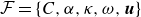 $\mathcal {F}=\{C,\alpha , \kappa , \omega , \boldsymbol {u}\}$
for the mesh adaption in our simulations. The resulting time variation of the lift coefficient
$\mathcal {F}=\{C,\alpha , \kappa , \omega , \boldsymbol {u}\}$
for the mesh adaption in our simulations. The resulting time variation of the lift coefficient
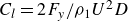 $C_{l}=2F_{y}/\rho _{1}U^{2}D$
is plotted in figure 18(a), where
$C_{l}=2F_{y}/\rho _{1}U^{2}D$
is plotted in figure 18(a), where
 $F_{y}$
is the vertical hydrodynamic load (excluding buoyancy) experienced by the cylinder. Hydrodynamic lift obtained from our quadtree-based simulations converges for the grid resolutions of
$F_{y}$
is the vertical hydrodynamic load (excluding buoyancy) experienced by the cylinder. Hydrodynamic lift obtained from our quadtree-based simulations converges for the grid resolutions of
 $\mathcal {L}_{h}=11$
and
$\mathcal {L}_{h}=11$
and
 $12$
, as indicated by overlapping curves in figure 18(a). In both cases, the lowest grid refinement level is kept at
$12$
, as indicated by overlapping curves in figure 18(a). In both cases, the lowest grid refinement level is kept at
 $\mathcal {L}_{l}=6$
. As one can notice, the lift force signal in figure 18(a) is biased towards negative values. This pronounced downward lift is a consequence of the nearby liquid–gas interface. The comparison of our time-averaged lift coefficient
$\mathcal {L}_{l}=6$
. As one can notice, the lift force signal in figure 18(a) is biased towards negative values. This pronounced downward lift is a consequence of the nearby liquid–gas interface. The comparison of our time-averaged lift coefficient
 $\overline {C}_{l}$
with the published results of Colagrossi et al. (Reference Colagrossi, Nikolov, Durante, Marrone and Souto-Iglesias2019) is provided in table 3. Moreover, an instantaneous vorticity field and the liquid–gas interface are shown in figure 18(b) at the instance of maximum lift in figure 18(a). Coefficient
$\overline {C}_{l}$
with the published results of Colagrossi et al. (Reference Colagrossi, Nikolov, Durante, Marrone and Souto-Iglesias2019) is provided in table 3. Moreover, an instantaneous vorticity field and the liquid–gas interface are shown in figure 18(b) at the instance of maximum lift in figure 18(a). Coefficient
 $\overline {C}_{l}$
and the observed interface deformation in our simulation closely align with the numerical findings of Colagrossi et al. (Reference Colagrossi, Nikolov, Durante, Marrone and Souto-Iglesias2019) (see table 3 and figure 18
b). Interested readers can further refer to figure 9 in Colagrossi et al. (Reference Colagrossi, Nikolov, Durante, Marrone and Souto-Iglesias2019) for a qualitative comparison of our vorticity field in figure 18(b).
$\overline {C}_{l}$
and the observed interface deformation in our simulation closely align with the numerical findings of Colagrossi et al. (Reference Colagrossi, Nikolov, Durante, Marrone and Souto-Iglesias2019) (see table 3 and figure 18
b). Interested readers can further refer to figure 9 in Colagrossi et al. (Reference Colagrossi, Nikolov, Durante, Marrone and Souto-Iglesias2019) for a qualitative comparison of our vorticity field in figure 18(b).
Table 3. Time-averaged lift coefficient
 $\overline {C}_{l}$
, amplitude
$\overline {C}_{l}$
, amplitude
 $C^{\prime }_{l}$
and non-dimensional frequency
$C^{\prime }_{l}$
and non-dimensional frequency
 $fD/U$
of the fluctuating lift force computed from the present VOF-based simulations on quadtree grids (
$fD/U$
of the fluctuating lift force computed from the present VOF-based simulations on quadtree grids (
 $\mathcal {L}_{h}=11$
and
$\mathcal {L}_{h}=11$
and
 $12$
) and the findings published by Colagrossi et al. (Reference Colagrossi, Nikolov, Durante, Marrone and Souto-Iglesias2019) using three different numerical schemes: smoothed particle hydrodynamics (SPH), level-set method (LSM) and VOF. The simulation parameters are
$12$
) and the findings published by Colagrossi et al. (Reference Colagrossi, Nikolov, Durante, Marrone and Souto-Iglesias2019) using three different numerical schemes: smoothed particle hydrodynamics (SPH), level-set method (LSM) and VOF. The simulation parameters are
 $\rho _{1}/\rho _{2}=1000$
,
$\rho _{1}/\rho _{2}=1000$
,
 $\mu _{1}/\mu _{2}=100$
,
$\mu _{1}/\mu _{2}=100$
,
 $L=40D$
,
$L=40D$
,
 $h=0.9D$
,
$h=0.9D$
,
 $ {Re}=180$
,
$ {Re}=180$
,
 $\sigma =0$
and
$\sigma =0$
and
 $ {Fr}=0.3$
.
$ {Fr}=0.3$
.


Figure 18. (a) Temporal evolution of the lift coefficient
 $C_{l}$
for
$C_{l}$
for
 $\rho _{1}/\rho _{2}=1000$
,
$\rho _{1}/\rho _{2}=1000$
,
 $\mu _{1}/\mu _{2}=100$
,
$\mu _{1}/\mu _{2}=100$
,
 $L=40D$
,
$L=40D$
,
 $h=0.9D$
,
$h=0.9D$
,
 $ {Re}=180$
,
$ {Re}=180$
,
 $\sigma =0$
and
$\sigma =0$
and
 $ {Fr}=0.3$
. Here
$ {Fr}=0.3$
. Here
 $\mathcal {L}_{h}$
indicates the highest refinement level of a quadtree mesh, and
$\mathcal {L}_{h}$
indicates the highest refinement level of a quadtree mesh, and
 $N$
denotes the number of uniformly spaced grid points per unit cylinder diameter
$N$
denotes the number of uniformly spaced grid points per unit cylinder diameter
 $D$
in figure 1. (b) Snapshot of the vorticity pattern around the cylinder and weakly deformed liquid–gas interface (green-coloured curve). Orange circles highlight the free surface profile extracted from Colagrossi et al. (Reference Colagrossi, Nikolov, Durante, Marrone and Souto-Iglesias2019). Note that Cartesian coordinates in (b) are in units of the cylinder diameter
$D$
in figure 1. (b) Snapshot of the vorticity pattern around the cylinder and weakly deformed liquid–gas interface (green-coloured curve). Orange circles highlight the free surface profile extracted from Colagrossi et al. (Reference Colagrossi, Nikolov, Durante, Marrone and Souto-Iglesias2019). Note that Cartesian coordinates in (b) are in units of the cylinder diameter
 $D$
.
$D$
.
In summary, a grid resolution of
 $N\approx 51$
adequately captures the flow within the gap between the cylinder and the liquid–gas interface and, thereby, hydrodynamic lift. However, for scenarios involving high Froude numbers where the liquid–gas interface breaks and very small droplets and bubbles form, we opt for a finer mesh resolution of
$N\approx 51$
adequately captures the flow within the gap between the cylinder and the liquid–gas interface and, thereby, hydrodynamic lift. However, for scenarios involving high Froude numbers where the liquid–gas interface breaks and very small droplets and bubbles form, we opt for a finer mesh resolution of
 $N\approx 102$
. This finer resolution allows us to resolve droplets and bubbles that are two orders of magnitude smaller than the cylinder. For two-dimensional simulations detailed in § 3, we expand our domain size to
$N\approx 102$
. This finer resolution allows us to resolve droplets and bubbles that are two orders of magnitude smaller than the cylinder. For two-dimensional simulations detailed in § 3, we expand our domain size to
 $L=80$
, doubling the current domain size while maintaining the resolution at
$L=80$
, doubling the current domain size while maintaining the resolution at
 $N\approx 102$
by setting
$N\approx 102$
by setting
 $\mathcal {L}_{h}=13$
. A larger flow domain is crucial to observe wake and interface dynamics far downstream from the cylinder. Throughout our simulations, we keep
$\mathcal {L}_{h}=13$
. A larger flow domain is crucial to observe wake and interface dynamics far downstream from the cylinder. Throughout our simulations, we keep
 $\epsilon$
and
$\epsilon$
and
 $\mathcal {F}$
the same as for the current test case. While surface tension modelling is not required for the current test case in figure 18, since
$\mathcal {F}$
the same as for the current test case. While surface tension modelling is not required for the current test case in figure 18, since
 $\sigma =0$
, it is worth noting that the Basilisk library has already been tested on several other stringent free-surface problems involving surface tension (Deike et al. Reference Deike, Popinet and Melville2015; Mostert et al. Reference Mostert, Popinet and Deike2022; Tang, Adcock & Mostert Reference Tang, Adcock and Mostert2024).
$\sigma =0$
, it is worth noting that the Basilisk library has already been tested on several other stringent free-surface problems involving surface tension (Deike et al. Reference Deike, Popinet and Melville2015; Mostert et al. Reference Mostert, Popinet and Deike2022; Tang, Adcock & Mostert Reference Tang, Adcock and Mostert2024).
Before closing our discussion, we add a couple of remarks. Firstly, in order to precisely resolve wake vortices and free-surface deformation across the entire downstream region, one cannot rely on conventional non-uniform grids, as employed in previous tFSI studies (Reichl et al. Reference Reichl, Hourigan and Thompson2005; Colagrossi et al. Reference Colagrossi, Nikolov, Durante, Marrone and Souto-Iglesias2019; Karmakar & Saha Reference Karmakar and Saha2020). In the current set-up, discretising the entire computational domain using a uniform Cartesian grid will yield
 ${\approx }67$
million grid cells. Thus, adaptive mesh refinement is likely the only viable alternative to resolve extended downstream regions accurately at an affordable computational cost. Secondly, our two-dimensional numerical formulation incorporates the potential form of the gravitational body force in (2.2), which has a mathematical structure similar to that of the surface tension body force (see Popinet (Reference Popinet2018) for further details). This is particularly advantageous for reducing spurious currents in free-surface flow simulations, as seen in Wroniszewski et al. (Reference Wroniszewski, Verschaeve and Pedersen2014).
${\approx }67$
million grid cells. Thus, adaptive mesh refinement is likely the only viable alternative to resolve extended downstream regions accurately at an affordable computational cost. Secondly, our two-dimensional numerical formulation incorporates the potential form of the gravitational body force in (2.2), which has a mathematical structure similar to that of the surface tension body force (see Popinet (Reference Popinet2018) for further details). This is particularly advantageous for reducing spurious currents in free-surface flow simulations, as seen in Wroniszewski et al. (Reference Wroniszewski, Verschaeve and Pedersen2014).
Appendix B. Interface breakup and coalescence in VOF simulations
In practice, the breakup and merging of fluid interfaces can be influenced by intermolecular forces, particularly when the gap between approaching interface segments shrinks to the nanometre scale. For instance, bubble-bursting experiments reveal that the film thickness at the moment of breakup typically measures a few micrometres, rendering the effects of intermolecular forces negligible in these cases (Lhuissier & Villermaux Reference Lhuissier and Villermaux2012). Conversely, experiments involving the collision of millimetric droplets demonstrate that as the droplets approach each other, the surrounding fluid in the gap is squeezed radially outward, reducing the gap between droplet interfaces to nanometre scales. At this point, van der Waals forces become dominant, driving the coalescence of the droplets (Chesters Reference Chesters1991).
In two-fluid simulations employing interface-capturing methods like the VOF, phase-field or level-set approaches, breakup and coalescence events are inherently numerical (Roccon et al. Reference Roccon, Zonta and Soldati2023). Interfaces break or coalesce when their separation falls below the grid size. As the grid resolution is refined, these numerical events converge towards the physical phenomena. This principle applies to existing numerical studies of bubble entrainment and droplet production caused by free-surface breaking (Deike et al. Reference Deike, Popinet and Melville2015, Reference Deike, Ghabache, Liger-Belair, Das, Zaleski, Popinet and Séon2018; Brasz et al. Reference Brasz, Bartlett, Walls, Flynn, Yu and Bird2018; Hendrickson et al. Reference Hendrickson, Weymouth, Yu and Yue2019; Yu et al. Reference Yu, Hendrickson, Campbell and Yue2019; Chan et al. Reference Chan, Johnson, Moin and Urzay2021; Mostert et al. Reference Mostert, Popinet and Deike2022; and many more). Despite the absence of intermolecular interactions in simulations, the numerical interface dynamics in such interface-resolved studies has shown good agreement with experimental and natural flow observations, albeit with the possibility of a slightly enhanced coalescence rate (Roccon et al. Reference Roccon, Zonta and Soldati2023). We point out that incorporating molecular-level effects often has minimal impact on the breakup and coalescence of interfaces, as these processes occur rapidly (Tryggvason et al. Reference Tryggvason, Scardovelli and Zaleski2011).
Drawing on prior works, we anticipate that our simulated breakup and coalescence dynamics will closely mirror real-world behaviour. Nevertheless, the precise answer to the potential role of intermolecular forces in the interface dynamics in the present set-up can only be assessed with the help of experimental investigations. Extreme scenarios requiring macroscopic flow to be resolved down to scales dominated by intermolecular forces remain virtually unattainable in traditional multi-phase flow simulations, even when using adaptive mesh refinement (Thomas, Esmaeeli & Tryggvason Reference Thomas, Esmaeeli and Tryggvason2010) and high-performance computing (Roccon et al. Reference Roccon, Zonta and Soldati2023).
Finally, in the gas entrainment regime, the smallest bubbles and droplets that current simulations can resolve with reasonable accuracy are approximately the size of the finest computational cell, a capability facilitated by the mass-preserving properties of the VOF framework (Scardovelli & Zaleski Reference Scardovelli and Zaleski1999; Popinet Reference Popinet2009; Yang et al. Reference Yang, Lu and Wang2021; Riviére et al. Reference Riviére, Mostert, Perrard and Deike2021).
Appendix C. Detection of entrained gas bubbles in CAS-Tank solver
In this study, the bubble identification technique introduced by Herrmann (Reference Herrmann2010) is employed to detect and characterise individual bubbles within a three-dimensional multi-phase flow simulation performed using the CAS-Tank solver (Yang et al. Reference Yang, Lu and Wang2021). The procedure initiates with an iterative algorithm that systematically traverses the domain, whereupon each detected bubble is assigned a unique identifier, denoted as
 $id$
, following the band generation method. This algorithm progressively expands from the initial seed point in concentric layers, encompassing adjacent cells until the entire continuous bubble structure is fully identified.
$id$
, following the band generation method. This algorithm progressively expands from the initial seed point in concentric layers, encompassing adjacent cells until the entire continuous bubble structure is fully identified.
Upon the completion of tagging a continuous bubble, the identifier
 $id$
is incremented, and the algorithm searches for the next untagged cell containing the gas phase to initiate the identification process for the subsequent bubble. This process continues until all bubbles within the domain have been uniquely labelled. A comprehensive lookup table is then generated, indexing all identified bubbles for further analysis.
$id$
is incremented, and the algorithm searches for the next untagged cell containing the gas phase to initiate the identification process for the subsequent bubble. This process continues until all bubbles within the domain have been uniquely labelled. A comprehensive lookup table is then generated, indexing all identified bubbles for further analysis.
The physical characteristics of the bubbles, including their volume, centre of mass and velocity, are subsequently calculated according to the following equations:
 \begin{align} V_{id} &= \sum _{\mathrm {tag}_i = id} F_i(B)V_{B_i}, \end{align}
 \begin{align} \boldsymbol {x}_{id} &= \frac {1}{V_{id}}\sum _{\mathrm {tag}_i = id} \boldsymbol {x}_i F_i(B) V_{B_i}, \end{align}
 \begin{align} \boldsymbol {u}_{id} &= \frac {1}{V_{id}}\sum _{\mathrm {tag}_i = id} \boldsymbol {u}_i F_i(B) V_{B_i}. \end{align}
Here, for a bubble tagged with
 $id$
, the symbol
$id$
, the symbol
 $B$
denotes the group of grid cells constituting the bubble. Also,
$B$
denotes the group of grid cells constituting the bubble. Also,
 $F_i(B)$
is the cell volume fraction within cell
$F_i(B)$
is the cell volume fraction within cell
 $i$
,
$i$
,
 $V_{B_i}$
represents the volume of cell
$V_{B_i}$
represents the volume of cell
 $i$
while
$i$
while
 $\boldsymbol {x}_{i}$
and
$\boldsymbol {x}_{i}$
and
 $\boldsymbol {u}_{i}$
denote the cell centroid coordinates and velocity of cell
$\boldsymbol {u}_{i}$
denote the cell centroid coordinates and velocity of cell
 $i$
, respectively.
$i$
, respectively.


 Open access