Hostname: page-component-745bb68f8f-g4j75 Total loading time: 0 Render date: 2025-01-11T03:38:16.053Z Has data issue: false hasContentIssue false

Arbitrary-order sensitivities of the incompressible base flow and its eigenproblem

Published online by Cambridge University Press:  23 April 2024

S.J. Knechtel*
Affiliation:
Laboratory for Flow Instabilities and Dynamics, ISTA, Technische Universität Berlin, 10623 Berlin, Germany
T.L. Kaiser
Affiliation:
Laboratory for Flow Instabilities and Dynamics, ISTA, Technische Universität Berlin, 10623 Berlin, Germany
A. Orchini*
Affiliation:
Nonlinear Thermo-Fluid Mechanics, ISTA, Technische Universität Berlin, 10623 Berlin, Germany
K. Oberleithner
Affiliation:
Laboratory for Flow Instabilities and Dynamics, ISTA, Technische Universität Berlin, 10623 Berlin, Germany
*
Email addresses for correspondence: s.knechtel@tu-berlin.de, a.orchini@tu-berlin.de

Abstract

First-order sensitivities and adjoint analysis are used widely to control the linear stability of unstable flows. Second-order sensitivities have recently helped to increase accuracy. In this paper, a method is presented to calculate arbitrary high-order sensitivities based on Taylor expansions of the incompressible base flow and its eigenproblem around a scalar parameter. For the incompressible Navier–Stokes equations, general expressions for the sensitivities are derived, into which parameter-specific information can be inserted. The computational costs are low since, for all orders, a linear equation system has to be solved, of which the left-hand-side matrix stays constant and thus its preconditioning can be exploited. Two flow scenarios are examined. First, the cylinder flow equations are expanded around the inverse of the Reynolds number, enabling the prediction of the two-dimensional cylinder base flow and its leading eigenvalue as a function of the Reynolds number. This approach computes accurately the base flow and eigenvalue even in the unstable regime, providing, when executed subsequently, a mean to calculate unstable base flows. This case gives a clear introduction into the method and allows us to discuss its constraints regarding convergence behaviour. Second, a small control cylinder is introduced into the domain of the cylinder flow for stabilization. Higher-order sensitivity maps are calculated by modelling the small cylinder with a steady forcing. These maps help to identify stabilizing areas of the flow field for Reynolds numbers within the laminar vortex shedding regime, with the required number of orders increasing as the Reynolds number rises. The results obtained through the proposed method align well with numerically calculated eigenvalues that incorporate the cylinder directly into the grid.

Type
JFM Papers
Copyright
© The Author(s), 2024. Published by Cambridge University Press

1. Introduction

In the last decades, adjoint methods have been used extensively in the field of fluid dynamics to compute flow gradient information with respect to a number of parameters, within the constraints of the Navier–Stokes equations. These methods are computationally convenient when compared to other gradient computation techniques – e.g. finite difference estimations – particularly when the sensitivity of the flow with respect to many control parameters is of interest (Baysal & Eleshaky Reference Baysal and Eleshaky1992). A prototypical application of adjoint methods is the calculation of the first-order sensitivity of the stability margins of a given flow configuration (Luchini & Bottaro Reference Luchini and Bottaro2014a). In particular, the stability properties of the flow past a circular cylinder, which often serves as a benchmark case for the analysis of hydrodynamic instabilities, has been investigated extensively. In a seminal work, Hill (Reference Hill1992) used adjoint stability analysis to re-stabilize the cylinder wake through passive control, by placing a small control cylinder into the cylinder wake. By using adjoint methods, Giannetti & Luchini (Reference Giannetti and Luchini2007) localized the most sensitive regions to momentum forcing or mass injection. In particular, by analysing the first-order sensitivity to a localized feedback mechanism that inserted a forcing proportional to the perturbation velocity, they achieved good qualitative agreement with experiments conducted by Strykowski & Sreenivasan (Reference Strykowski and Sreenivasan1990), who traced the regions in which a small control cylinder had a stabilizing effect. Marquet, Sipp & Jacquin (Reference Marquet, Sipp and Jacquin2008) formalized the calculation of the first-order sensitivity to base flow modifications. By introducing a steady forcing proportional to the base flow velocity, they refined predictions regarding the small control cylinder. These sensitivity calculations could also be performed on non-stationary solutions, e.g. on limit cycle oscillations, as discussed in Giannetti, Camarri & Citro (Reference Giannetti, Camarri and Citro2019).

All the aforementioned studies are based on a gradient (first-order sensitivity) analysis. While first-order sensitivities provide a good insight into the development of the flow properties while varying a certain parameter, and can be used for gradient-based optimization, evaluating second-order sensitivities is necessary for some flow configurations. This is the case, e.g. for configurations with symmetry properties, in which the first-order sensitivity vanishes. For example, Hwang, Kim & Choi (Reference Hwang, Kim and Choi2013) investigated a two-dimensional wake with a spanwise wavy perturbation of the base flow. They first observed that the sensitivity of the eigenvalue is proportional to the square of the perturbation amplitude, thus rendering the first-order sensitivity zero. Del Guercio, Cossu & Pujals (Reference Del Guercio, Cossu and Pujals2014) obtained analogous results. Tammisola et al. (Reference Tammisola, Giannetti, Citro and Juniper2014) first computed the second-order sensitivity of the eigenvalue for the purpose of controlling the cylinder wake flow with steady spanwise wavy actuation. Boujo, Fani & Gallaire (Reference Boujo, Fani and Gallaire2015Reference Boujo, Fani and Gallaire2019) computed the second-order sensitivity for parallel shear flows and the circular cylinder, respectively, by investigating the effect of spanwise waviness. Tammisola (Reference Tammisola2017) conducted a spanwise shape optimization of the cylinder, where the shape contour was parametrized with more than one parameter, and the second-order Hessian matrix was computed.

The importance of second-order (and higher-order) sensitivities is, however, not limited to scenarios with zero gradient. First-order sensitivity provides only gradient (linear) information on the overall sensitivity, i.e. it is accurate only for infinitesimally small variations of a parameter. To assess the effect that a real-world finite variation of a parameter has on the base flow/eigenvalues, higher-order (nonlinear) sensitivities are useful. Assessing in one high-order calculation the effect of a large variation of a parameter can reduce computational costs compared to assessing the same effect with many first-order linear steps. To obtain equations for the high-order sensitivities, one can exploit perturbation theory (Van Dyke Reference Van Dyke1975). Perturbation theory allows one to derive polynomial approximations to the variation of a flow quantity with respect to a parameter. This results in the construction of a series whose coefficients need to be evaluated order by order. As for any power series, the obtained series do not necessarily converge for arbitrarily large values of the perturbation parameter, but have a region of convergence, which may or may not be small (Bender & Orszag Reference Bender and Orszag1999). It is a general result of perturbation theory that within the region of convergence, the higher the perturbation order, the more accurate the results.

In this study, we present a perturbation theory framework for the computation of arbitrary high-order sensitivities for the incompressible Navier–Stokes equations with respect to a scalar parameter, together with a discussion on the convergence properties of the obtained solutions. The perturbation framework is applied to three classic problems: (i) the evaluation of base flows while varying the Reynolds number; (ii) the variation of the eigenvalues as the Reynolds number is increased; (iii) the influence of a passive forcing on the stability margins of the cylinder flow.

1.1. Base flow sensitivity to the Reynolds number

The computation of steady-state (time-independent) solutions of the nonlinear Navier–Stokes operator can be challenging for globally unstable flow fields. In these cases, classic pseudo-time-marching schemes fail, since the solution naturally diverges from the base flow configuration. A common valid alternative is the use of Newton-like methods. These methods do usually converge but may require a relatively accurate initial guess and thus a large number of steps. An alternative approach is the method of selective frequency damping (Akervik et al. Reference Akervik, Brandt, Henningson, Hoepffner, Marxen and Schlatter2006). This method can be integrated into pseudo-time-marching schemes and is therefore particularly suitable for large flow problems. Nevertheless, Jordi, Cotter & Sherwin (Reference Jordi, Cotter and Sherwin2015) and Casacuberta et al. (Reference Casacuberta, Groot, Tol and Hickel2018) pointed out shortcomings regarding its application to unstable systems with a steady unstable eigenmode or more than one unstable mode.

In this study, we employ perturbation theory to derive equations for the computation of the base flow modifications at arbitrarily high orders when a parameter (notably the Reynolds number) is varied. With this approach it is possible to get a continuous power series representation of the base flow solution along the parameter, within a convergence region. We then show how the higher-order base flow corrections can be used as an alternative method to obtain base flow solutions of globally unstable flows. Starting from a stable configuration (at low Reynolds number), the perturbation scheme allows us to obtain an accurate solution to a higher Reynolds number – within the region of convergence. The residuum of the Navier–Stokes equations is used to ensure sufficient accuracy. By repeating this process multiple times, we can extend the initial solution to an arbitrarily high Reynolds number. As a result, our method provides a continuous representation of the solution space. It is also similar to the more classic continuation methods, with the difference that continuation methods use only first-order gradient information – thus require small steps – whereas the proposed method uses larger steps, which is possible because higher-order sensitivity information is available.

1.2. Eigenvalue sensitivity, including base flow variations

When varying the Reynolds number, not only the base flow varies, but also the eigenvalues that govern its stability move in the complex plane. By using adjoint-based perturbation theory, it is possible to obtain a power series representation of the dependency of the eigenvalue trajectories on the parameter that, within the region of convergence, accurately approximates the actual eigenvalues. This was demonstrated recently by Mensah, Orchini & Moeck (Reference Mensah, Orchini and Moeck2020) and Orchini et al. (Reference Orchini, Magri, Silva, Mensah and Moeck2020) in a compressible-flow configuration relevant for thermoacoustic applications in which the base flow was frozen. It is, however, known that a variation in the base flow affects the stability of the flow (see e.g. Luchini & Bottaro Reference Luchini and Bottaro2014a). When varying the Reynolds number, therefore, the eigenvalue sensitivity needs to account for two effects: (i) a direct influence of the Reynolds number on the eigenvalues, and (ii) an indirect influence on the eigenvalues caused by the variation of the base flow induced by a change in the Reynolds number. The first-order expressions for the (total) eigenvalue sensitivity are known; see e.g. Marquet et al. (Reference Marquet, Sipp and Jacquin2008). The expression for the second-order sensitivity was given in Boujo (Reference Boujo2021). However, general expressions for the higher-order eigenvalue sensitivity accounting for the base flow modifications are, to the best knowledge of the authors, not available in the literature. In this study, we employ adjoint-based perturbation theory to derive the eigenvalue corrections, including base flow modifications to an arbitrarily high expansion order. In the process, we demonstrate how the base flow perturbation terms feed into the eigenvalue sensitivity problem, order by order. This implies that the convergence region of the eigenvalue expansions may be limited by the convergence of the base flow expansions, as will be discussed.

1.3. Effect of a passive forcing on the stability margin

The relevance of second-order sensitivity for flow problems was demonstrated recently by Boujo (Reference Boujo2021), who investigated the second-order influence of a perturbation in the cylinder wake imposed by a steady forcing, a flow configuration in which the first order does not vanish. By applying second-order sensitivity analysis, it was shown how the predictions of stabilizing regions may vary significantly and compare better to the experimental results of Strykowski & Sreenivasan (Reference Strykowski and Sreenivasan1990). An important remark is that this analysis assumes implicitly that the first- and second-order sensitivities can be summed straightforwardly. Since the derivation of first- and second-order sensitivities relies on adjoint-based perturbation techniques, care must be taken in summing the results. Perturbation solutions, in fact, generally converge not everywhere, but only within a certain parameter range (Bender & Orszag Reference Bender and Orszag1999). Being aware of this limitation is important when considering high-order expansions, because one has to verify if the constructed power series actually converges. In this study, we extend the analysis of Boujo (Reference Boujo2021) to higher orders, and we demonstrate that within the region of convergence, the high-order power series agree with high accuracy with the numerically obtained results when incorporating a small control cylinder directly into the grid.

1.4. Outline

The paper is structured as follows. In § 2, expressions for arbitrary-order sensitivities of the base flow of the Navier–Stokes equations with respect to one scalar parameter are derived. In § 3, adjoint-based perturbation methods are used to obtain high-order sensitivities of the eigenvalues of the linearized base flow equations, accounting for the base flow modification effects. The numerical set-up of the cylinder base flow, which is chosen to demonstrate the validity of the theory, is explained in § 4. The inverse of the Reynolds number serves as the scalar parameter of the first expansion case. In § 5.1, a base flow and eigenvalue prediction through a Taylor expansion around Reynolds number 47 is shown. In § 5.2, the cylinder base flow is subsequently calculated up to high Reynolds numbers, and the base flow and eigenvalues are traced until Reynolds number 1000. In § 5.3, some aspects of the convergence behaviour of the obtained power series approximations are discussed. As a second example case, higher-order sensitivity maps along the amplitude of a steady forcing are drawn in § 6, which serve as a model for the passive flow control of a small control cylinder that is placed inside the domain. The conclusions of the work are summarized in § 7.

2. Arbitrary-order sensitivities of the base flow

Consider the stationary incompressible Navier–Stokes (NS) equations

(2.1)\begin{equation} \boldsymbol{N}(\boldsymbol{q})\equiv\left(\begin{array}{@{}c@{}} (\boldsymbol{u}\boldsymbol{\cdot}\boldsymbol{\nabla})\boldsymbol{u}+\boldsymbol{\nabla} p-\dfrac{1}{{{Re}}}\,\nabla^{2}\boldsymbol{u}\\ \boldsymbol{\nabla}\boldsymbol{\cdot}\boldsymbol{u} \end{array}\right)=\boldsymbol{0}\end{equation}

and their solution $\boldsymbol {q}$, in the following called the ‘base flow’,

(2.2)\begin{equation} \boldsymbol{q}(\boldsymbol{x})\equiv\left(\begin{array}{@{}c@{}} \boldsymbol{u}(\boldsymbol{x})\\ p(\boldsymbol{x}) \end{array}\right)\!, \end{equation}

where $p(\boldsymbol {x})$ is the relative pressure, and $\boldsymbol {u}(\boldsymbol {x})\equiv (u(\boldsymbol {x}),v(\boldsymbol {x}))^{\rm T}$ is the velocity vector, here in this cylinder set-up in two dimensions, but generally having three velocity components. The Reynolds number ${{Re}}\equiv {u_{\infty }D}/{\nu }$ is defined by a characteristic velocity $u_{\infty }$, a characteristic length scale $D$, and a constant kinematic viscosity $\nu$, and the NS equations are made dimensionless with these characteristic quantities.

Consider now a scalar parameter $a$, which changes the NS equations and thus also the base flow via

(2.3)\begin{equation} \boldsymbol{N}(\boldsymbol{q}(a),a)=\boldsymbol{0}. \end{equation}

We are interested in the higher-order sensitivities of the base flow with regard to this parameter $a$. Expanding $\boldsymbol {q}$ in a Taylor polynomial of order $n$ around $a_{0}$ yields

(2.4)\begin{equation} {\boldsymbol{q}(a)\approx\boldsymbol{q}^{(n)}(a_{0}+\epsilon)=\boldsymbol{q}^{(n)}(a)\equiv\sum_{k=0}^{n}\dfrac{1}{k!}\, \boldsymbol{q}_{k} \epsilon^{k}}, \end{equation}

with $\epsilon = a-a_0$, and $a$ being in the vicinity of $a_0$. In the limit $n\rightarrow \infty$, the series (2.4) is guaranteed to converge asymptotically within the (a priori unknown) radius of the convergence $r$, i.e. if $|\epsilon |< r$ (Bender & Orszag Reference Bender and Orszag1999). For a finite value of $n$, however, the truncated series may nonetheless provide a good approximation even outside of the radius of convergence, a fact also known as Carrier's rule (Boyd Reference Boyd1999). The coefficients $\boldsymbol {q}_{k}$ are defined as

(2.5)\begin{equation} \boldsymbol{q}_{k}\equiv\left.\frac{\text{d}^{k}\boldsymbol{q}(a)}{(\text{d}a)^{k}}\right|_{a=a_{0}}. \end{equation}

For the incompressible NS equations, the Taylor polynomial reads

(2.6)\begin{equation} \boldsymbol{N}(\boldsymbol{q}(a),a)\approx\boldsymbol{N}{}^{(n)}(\boldsymbol{q}(a),a)\equiv\sum_{k=0}^{n}\dfrac{1}{k!}\, \boldsymbol{N}_{k}\epsilon^{k}=\boldsymbol{0}.\end{equation}

According to (2.1) and (2.3), (2.6) vanishes for all $a$ and $\boldsymbol {q}(a)$ by definition, which also implies that for each $k$, it must hold that $\boldsymbol {N}_{k}=\boldsymbol 0$.

2.1. Taylor coefficients for the base flow

We now show how the Taylor coefficients, i.e. the higher-order sensitivities of the base flow with respect to $a$, can be computed. In this subsection, the scalar parameter $a$ will be kept generic. We start with a detailed discussion on the first- and second-order coefficients, before presenting a general formulation for coefficients of arbitrary order.

The first-order sensitivity of $\boldsymbol {N}$ towards $a$ is

(2.7)\begin{align} \boldsymbol{N}_{1}\equiv\left.\frac{\text{d}\boldsymbol{N}(\boldsymbol{q}(a),a)}{\text{d}a}\right|_{a=a_{0}}=\left.\frac{\partial\boldsymbol{N}(\boldsymbol{q}(a),a_{0})}{\partial\boldsymbol{q}}\right|_{\boldsymbol{q}(a)=\boldsymbol{q}_{0}}\left.\frac{\text{d}\boldsymbol{q}(a)}{\text{d}a}\right|_{a=a_{0}}+\left.\frac{\partial\boldsymbol{N}(\boldsymbol{q}_{0},a)}{\partial a}\right|_{a=a_{0}}, \end{align}

where $\boldsymbol {q}_{0}$ is the base flow that solves (2.3) when $a=a_{0}$. For reasons of brevity, we replace the partial derivatives with subscripts from now on, and rewrite (2.7) as

(2.8)\begin{equation} \boldsymbol{N}_{1}\equiv\boldsymbol{N}_{\boldsymbol{q}}\boldsymbol{q}_{1}+\boldsymbol{N}_{a}=\boldsymbol 0. \end{equation}

Here, ${\boldsymbol {N}_{\boldsymbol {q}}}$ is the linearization of the NS equations with respect to $\boldsymbol {q}$ at $\boldsymbol {q}_{0}$, thus a linear operator or a tensor of order two, which explicitly reads

(2.9)\begin{equation} \boldsymbol{N}_{\boldsymbol{q}}\boldsymbol{q}_{k}=\left(\begin{array}{@{}c@{}} (\boldsymbol{u}_{0}\boldsymbol{\cdot}\boldsymbol{\nabla})\boldsymbol{u}_{k}+(\boldsymbol{u}_{k}\boldsymbol{\cdot}\boldsymbol{\nabla})\boldsymbol{u}_{0}+\boldsymbol{\nabla} p_{k}-\dfrac{1}{{{Re}}}\,\nabla^{2}\boldsymbol{u}_{k}\\ \boldsymbol{\nabla}\boldsymbol{\cdot}\boldsymbol{u}_{k} \end{array}\right) \end{equation}

when applied on any $\boldsymbol {q}_{k}$. The explicit expression for $\boldsymbol {N}_a$ depends on the parameter chosen for the expansion, as discussed later.

The first-order sensitivity of $\boldsymbol {q}$ towards $a$ can now be obtained by solving the linear system

(2.10)\begin{equation} \boldsymbol{N}_{\boldsymbol{q}}\boldsymbol{q}_{1}=-\boldsymbol{N}_{a}. \end{equation}

The first-order Taylor polynomial then reads

(2.11)\begin{equation} \boldsymbol{q}(a)\approx\boldsymbol{q}^{(1)}(a_{0}+\epsilon)=\boldsymbol{q}_{0}+\boldsymbol{q}_{1} \epsilon. \end{equation}

Following an analogous procedure, the equation for the second-order expansion reads

(2.12)\begin{equation} \boldsymbol{N}_{2}=\boldsymbol{N}_{\boldsymbol{q}}\boldsymbol{q}_{2}+\boldsymbol{q}_{1}^{\rm T}\boldsymbol{N}_{\boldsymbol{qq}}\boldsymbol{q}_{1}+2\boldsymbol{N}_{\boldsymbol{q}a}\boldsymbol{q}_{1}+\boldsymbol{N}_{aa}=\boldsymbol 0,\end{equation}

where $\boldsymbol {N}_{\boldsymbol {qq}}$ is a symmetric bilinear form or a tensor of order three that reads

(2.13)\begin{equation} \boldsymbol{q}_{j}^{\rm T}\boldsymbol{N}_{\boldsymbol{qq}}\boldsymbol{q}_{k}=\left(\begin{array}{@{}c@{}} (\boldsymbol{u}_{j}\boldsymbol{\cdot}\boldsymbol{\nabla})\boldsymbol{u}_{k}+(\boldsymbol{u}_{k}\boldsymbol{\cdot}\boldsymbol{\nabla})\boldsymbol{u}_{j}\\[3pt] 0 \end{array}\right) \end{equation}

when applied on any $\boldsymbol {q}_{j}$ and $\boldsymbol {q}_{k}$. We will provide explicit expressions for $\boldsymbol {N}_{\boldsymbol {q}a}$ and $\boldsymbol {N}_{aa}$ later when we specify $a$. We obtain the second-order sensitivity of $\boldsymbol {q}$ with respect to $a$ by solving the linear equation system

(2.14)\begin{equation} \boldsymbol{N}_{\boldsymbol{q}}\boldsymbol{q}_{2}=-\boldsymbol{q}_{1}^{\rm T}\boldsymbol{N}_{\boldsymbol{qq}}\boldsymbol{q}_{1}-2\boldsymbol{N}_{\boldsymbol{q}a}\boldsymbol{q}_{1}-\boldsymbol{N}_{aa}, \end{equation}

and the Taylor polynomial of order 2 is complete with

(2.15)\begin{equation} \boldsymbol{q}(a)\approx\boldsymbol{q}^{(2)}(a_{0}+\epsilon)=\boldsymbol{q}_{0}+\boldsymbol{q}_{1} \epsilon+\tfrac{1}{2}\,\boldsymbol{q}_{2} \epsilon^{2}. \end{equation}

This procedure can be pursued until arbitrary order. To obtain a general expression, it comes in handy that the higher-order derivatives of the NS equations with respect to the base flow vanish, i.e. that we have

(2.16)\begin{equation} \boldsymbol{N}_{\boldsymbol{qqq}}=\boldsymbol{0}=\boldsymbol{N}_{\boldsymbol{qqq}a}=\boldsymbol{N}_{\boldsymbol{qqqq}}=\cdots. \end{equation}

A closed formula for the computation of $\boldsymbol {q}_{k}$ for any scalar parameter $a$ then reads

(2.17) \begin{align} \boldsymbol{N}_{\boldsymbol{q}}\boldsymbol{q}_{k} & =-\sum_{i=1}^{k-2} \sum_{j=1}^{k-i-1}\left(\begin{array}{@{}c@{}} k\\ i \end{array}\right)\left(\begin{array}{@{}c@{}} k-i\\ j \end{array}\right)\frac{1}{2}\,\boldsymbol{q}_{j}^{\rm T}\boldsymbol{N}_{\boldsymbol{qq}a^{i}}\boldsymbol{q}_{k-i-j}\ \nonumber\\ & \quad-\sum_{i=1}^{k-1}\left(\begin{array}{@{}c@{}} k\\ i \end{array}\right)\left[\frac{1}{2}\,\boldsymbol{q}_{i}^{\rm T}\boldsymbol{N}_{\boldsymbol{qq}}\boldsymbol{q}_{k-i}+\boldsymbol{N}_{\boldsymbol{q}a^{i}}\boldsymbol{q}_{k-i}\right]-\boldsymbol{N}_{a^{k}}, \end{align}

where we adopted the notation $\boldsymbol {N}_{aa}=\boldsymbol {N}_{a^{2}}$ and so on for higher-order derivatives. The individual $\boldsymbol {q}_{k}$ have to be calculated one after the other from $k=1$ until $k=n$, the order of the desired Taylor polynomial. Note that the left-hand side of each linear equation system always contains the same linear operator $\boldsymbol {N}_{\boldsymbol {q}}$, which is advantageous for a fast computation of several higher orders.

2.2. Expansion of the equations with respect to the parameter $1/{{Re}}$

We will now specify the parameter $a$ as the inverse of the Reynolds number

(2.18)\begin{equation} a=\frac{1}{{{Re}}}, \end{equation}

and define explicit expressions for the operators defined in § 2.1. This choice for the parameter $a$ is convenient because $1/{{Re}}$ enters linearly in the NS equation. The case $a={{Re}}$ is also briefly discussed in this study and can be found in Appendix A. The first partial derivative of the NS equations (2.1) with respect to $a$ is

(2.19)\begin{equation} \boldsymbol{N}_{a}=\left(\begin{array}{@{}c@{}} -\nabla^{2}\boldsymbol{u}\\[2pt] 0 \end{array}\right), \end{equation}

and the higher order derivatives follow with

(2.20)\begin{equation} \boldsymbol{N}_{aa}=\boldsymbol{N}_{aaa}=\cdots=\boldsymbol{0}. \end{equation}

Similarly, the first partial derivative of the linear operator (2.9) with respect to $a$ is

(2.21)\begin{equation} \boldsymbol{N}_{\boldsymbol{q}a}\boldsymbol{q}_{k}=\left(\begin{array}{@{}c@{}} -\nabla^{2}\boldsymbol{u}_{k}\\[2pt] 0 \end{array}\right) \end{equation}

and for the higher orders,

(2.22)\begin{equation} \boldsymbol{N}_{\boldsymbol{q}aa}=\boldsymbol{N}_{\boldsymbol{q}aaa}=\cdots=\boldsymbol{0}. \end{equation}

Furthermore, it holds that

(2.23)\begin{equation} \boldsymbol{N}_{\boldsymbol{qq}a}=\boldsymbol{N}_{\boldsymbol{qq}aa}=\cdots=\boldsymbol{0}. \end{equation}

For the case $a=1/{{Re}}$, (2.17) thus simplifies to

(2.24)\begin{equation} \boldsymbol{N}_{\boldsymbol{q}}\boldsymbol{q}_{k}=\left\{ \begin{array}{@{}ll} -\boldsymbol{N}_{a}, & \text{for}\ k=1,\\ -\left(\begin{array}{@{}c@{}} k\\ 1 \end{array}\right)\boldsymbol{N}_{\boldsymbol{q}a}\boldsymbol{q}_{k-1} -\dfrac{1}{2}\displaystyle\sum_{i=1}^{k-1}\left(\begin{array}{@{}c@{}} k\\ i \end{array}\right)\boldsymbol{q}_{i}^{\rm T}\boldsymbol{N}_{\boldsymbol{qq}} \boldsymbol{q}_{k-i}, & \text{for}\ k>1 . \end{array}\right. \end{equation}

3. Arbitrary-order sensitivities of the eigenvalues

In the following, adjoint-based perturbation methods are used to obtain the arbitrary-order sensitivities of the eigenvalues of the linearized base flow equations with respect to one scalar parameter. The base flow sensitivities, which were derived in the previous section, are needed here to account for the base flow modifications that the parameter causes. In the following, we will assume that the eigenvalue(s) that we track are simple, i.e. not degenerate. For these eigenvalues, it can be shown formally that the radius of convergence of a Taylor series expansion is greater than zero (Lancaster, Markus & Zhou Reference Lancaster, Markus and Zhou2003).

The linear stability of the base flow is determined by the eigenvalues of the linear operator of the NS equations. The base flow is linearly unstable if at least one eigenvalue has a positive real part. The eigenproblem can be written as

(3.1)\begin{equation} \left(\boldsymbol{\mathsf{L}}(\boldsymbol{q})-\lambda\boldsymbol{\mathsf{M}}\right)\hat{\boldsymbol{q}}=\boldsymbol{0} ,\quad\hat{\boldsymbol{q}}=\left(\begin{array}{@{}c@{}} \hat{\boldsymbol{u}}\\ \hat{p} \end{array}\right) ,\end{equation}

where $\boldsymbol{\mathsf{L}}\equiv \boldsymbol {N}_{\boldsymbol {q}}$ from (2.9), and

(3.2)\begin{equation} \lambda\boldsymbol{\mathsf{M}}\hat{\boldsymbol{q}}=\lambda\left(\begin{array}{@{}c@{}} \hat{\boldsymbol{u}}\\ 0 \end{array}\right)\!. \end{equation}

An adjoint eigenproblem can be defined by introducing the adjoint operator $\boldsymbol{\mathsf{L}}^{*}$ as

(3.3)\begin{equation} \left(\boldsymbol{\mathsf{L}}^{*}(\boldsymbol{q})-\lambda{^*}\boldsymbol{\mathsf{M}}\right)\hat{\boldsymbol{q}}^{*}=\boldsymbol{0}, \end{equation}

with

(3.4)\begin{equation} \boldsymbol{\mathsf{L}}^{*}(\boldsymbol{q})\,\hat{\boldsymbol{q}}^{*}=\left(\begin{array}{@{}c@{}} (\boldsymbol{\nabla}\boldsymbol{u})\hat{\boldsymbol{u}}^{*}-(\boldsymbol{\nabla}\hat{\boldsymbol{u}}^{*})^{\rm T}\boldsymbol{u}-\boldsymbol{\nabla}\hat{p}^{*}-\dfrac{1}{{{Re}}}\,\nabla^{2}\hat{\boldsymbol{u}}^{*}\\ -\boldsymbol{\nabla}\boldsymbol{\cdot}\hat{\boldsymbol{u}}^{*} \end{array}\right)\!. \end{equation}

Consider again the scalar parameter $a$: a variation in $a$ changes not only the NS equations and the base flow, but also the eigenproblem:

(3.5)\begin{equation} \left[\boldsymbol{\mathsf{L}}(\boldsymbol{q}(a),a) - \lambda(a)\,\boldsymbol{\mathsf{M}}\right] \hat{\boldsymbol{q}}(a)=\boldsymbol 0. \end{equation}

We proceed as in the previous section by expanding $\lambda$, $\hat {\boldsymbol {q}}$ and $\boldsymbol{\mathsf{L}}$ into Taylor polynomials of order $n$. The Taylor polynomial for the eigenvalue $\lambda$ reads

(3.6)\begin{equation} \lambda(a)\approx\lambda^{(n)}(a_{0}+\epsilon)=\lambda^{(n)}(a)\equiv\sum_{k=0}^{n}\frac{1}{k!}\, \lambda_{k} \epsilon^{k},\end{equation}

with

(3.7)\begin{equation} \lambda_{k}=\left.\frac{\text{d}^{k}\lambda(a)}{(\text{d}a)^{k}}\right|_{a=a_{0}}, \end{equation}

and analogously for the eigenvector $\hat {\boldsymbol {q}}$,

(3.8)\begin{equation} \hat{\boldsymbol{q}}(a)\approx\hat{\boldsymbol{q}}^{(n)}(a) \equiv\sum_{k=0}^{n}\frac{1}{k!}\, \hat{\boldsymbol{q}}_{k} \epsilon^{k}, \end{equation}

and for the linear operator $\boldsymbol{\mathsf{L}}$,

(3.9)\begin{equation} \boldsymbol{\mathsf{L}}(\boldsymbol{q}(a),a)\approx\boldsymbol{\mathsf{L}}^{(n)}(\boldsymbol{q}(a),a)\equiv\sum_{k=0}^{n}\frac{1}{k!}\, \boldsymbol{\mathsf{L}}_{k} \epsilon^{k}. \end{equation}

Note that (3.6) and (3.8) hold only within a radius of convergence around $a_0$, as was explained for the Taylor expansion of the base flow. The radius of convergence for the eigenvalue expansion is limited by singularities, which include exceptional points (EPs) in the spectrum of the considered operator (Kato Reference Kato1980). The EPs are spectral singularities at which not only two (or more) eigenvalues coalesce, becoming degenerate, but also two (or more) eigenvectors coalesce, causing the linear operator to be defective. The EPs are expected to be found for complex-valued parameters, making also the linear operator complex-valued, implying that they are often not physically realizable (Seyranian, Kirillov & Mailybaev Reference Seyranian, Kirillov and Mailybaev2005). Still, their existence in the complex plane poses limits to the convergence of perturbation expansions.

3.1. Taylor coefficients for the linear operator

In the following, we will express the higher-order sensitivities of $\boldsymbol{\mathsf{L}}$ through partial derivatives of $\boldsymbol {N}$ that were defined in § 2. Because we have defined $\boldsymbol{\mathsf{L}}\equiv \boldsymbol {N}_{\boldsymbol {q}}$, it follows that $\boldsymbol{\mathsf{L}}_{q}=\boldsymbol {N}_{\boldsymbol {qq}}$, $\boldsymbol{\mathsf{L}}_{a}=\boldsymbol {N}_{\boldsymbol {q}a}$, and so on. Thus it can be found that at first order,

(3.10)\begin{equation} \boldsymbol{\mathsf{L}}_{1}\boldsymbol{q}_{j}=\boldsymbol{q}_{1}^{\rm T}\boldsymbol{N}_{\boldsymbol{qq}}\boldsymbol{q}_{j}+\boldsymbol{N}_{\boldsymbol{q}a}\boldsymbol{q}_{j},\end{equation}

and for second order,

(3.11)\begin{equation} \boldsymbol{\mathsf{L}}_{2}\boldsymbol{q}_{j}=\boldsymbol{q}_{2}^{\rm T}\boldsymbol{N}_{\boldsymbol{qq}}\boldsymbol{q}_{j}+2 \boldsymbol{q}_{1}^{\rm T}\boldsymbol{N}_{\boldsymbol{qq}a}\boldsymbol{q}_{j}+\boldsymbol{N}_{\boldsymbol{q}aa}\boldsymbol{q}_{j} .\end{equation}

The arbitrary-order expression takes the form

(3.12)\begin{equation} \boldsymbol{\mathsf{L}}_{k}\boldsymbol{q}_{j}=\boldsymbol{q}_{k}^{\rm T}\boldsymbol{N}_{\boldsymbol{qq}}\boldsymbol{q}_{j}+\sum_{i=1}^{k-1}\left(\begin{array}{@{}c@{}} k\\ i \end{array}\right)\boldsymbol{q}_{k-i}^{\rm T}\boldsymbol{N}_{\boldsymbol{qq}a^{i}}\boldsymbol{q}_{j}+\boldsymbol{N}_{qa^{k}}\boldsymbol{q}_{j}.\end{equation}

3.2. Taylor coefficients for the eigenvalue

The sensitivities of $\lambda (a)$ are derived by calculating the sensitivities towards $a$ of (3.1). The first-order eigenvalue sensitivity towards $a$, $\lambda _{1}$, is given by the sesquilinear scalar product

(3.13)\begin{equation} \lambda_{1}=\frac{1}{c}\left\langle\hat{\boldsymbol{q}}_{0}^{*},\boldsymbol{\mathsf{L}}_{1}\hat{\boldsymbol{q}}_{0}\right\rangle,\quad c\equiv\langle\hat{\boldsymbol{q}}_{0}^{*} ,\boldsymbol{\mathsf{M}}\hat{\boldsymbol{q}}_{0}\rangle .\end{equation}

This expression can be derived by calculating the first-order sensitivity towards $a$ at $a_{0}$ of the eigenproblem (3.1),

(3.14)\begin{equation} \left(\boldsymbol{\mathsf{L}}_{0}-\lambda_{0}\boldsymbol{\mathsf{M}}\right)\hat{\boldsymbol{q}}_{1}+\left(\boldsymbol{\mathsf{L}}_{1}-\lambda_{1}\boldsymbol{\mathsf{M}}\right)\hat{\boldsymbol{q}}_{0}=\boldsymbol{0},\end{equation}

and then taking the scalar product with the corresponding zeroth-order adjoint eigenvector; see e.g. Luchini & Bottaro (Reference Luchini and Bottaro2014b). From (3.3), it holds that

(3.15)\begin{equation} \left\langle\hat{\boldsymbol{q}}_{0}^{*},\left(\boldsymbol{\mathsf{L}}_{0}-\lambda_{0}\boldsymbol{\mathsf{L}}\right)\hat{\boldsymbol{q}}_{k}\right\rangle= 0 \end{equation}

for any $k$, therefore $\lambda _{1}$ can be calculated without knowing $\hat {\boldsymbol {q}}_{1}$.

The second-order sensitivity is derived in the exact same manner, i.e. by calculating the second-order sensitivity of (3.1) and then taking the scalar product with the corresponding zeroth-order adjoint eigenvector (Orchini et al. Reference Orchini, Magri, Silva, Mensah and Moeck2020; Boujo Reference Boujo2021):

(3.16)\begin{equation} \lambda_{2}=\frac{1}{c}\left\langle\hat{\boldsymbol{q}}_{0}^{*} ,\boldsymbol{\mathsf{L}}_{2}\hat{\boldsymbol{q}}_{0}\right\rangle+\frac{2}{c}\left\langle\hat{\boldsymbol{q}}_{0}^{*} ,\left(\boldsymbol{\mathsf{L}}_{1}-\lambda_{1}\boldsymbol{\mathsf{M}}\right)\hat{\boldsymbol{q}}_{1}\right\rangle .\end{equation}

Here, the first-order coefficient of the eigenvector, $\hat {\boldsymbol {q}}_{1}$, is needed, which will be derived in the next subsection. This procedure can be followed until arbitrary order, arriving at

(3.17)\begin{equation} \lambda_{k}=\frac{1}{c}\left\langle\hat{\boldsymbol{q}}_{0}^{*} ,\boldsymbol{\mathsf{L}}_{k}\hat{\boldsymbol{q}}_{0}\right\rangle+\frac{1}{c}\sum_{i=1}^{k-1}\left(\begin{array}{@{}c@{}} k\\ i \end{array}\right)\left\langle\hat{\boldsymbol{q}}_{0}^{*} ,\left(\boldsymbol{\mathsf{L}}_{i}-\lambda_{i}\boldsymbol{\mathsf{M}}\right)\hat{\boldsymbol{q}}_{(k-i)}\right\rangle . \end{equation}

Note that the respective lower-order sensitivities of the eigenvalue and the eigenvector have to be known beforehand, which means that higher-order eigenvalue coefficients have to be calculated one after the other.

3.3. Taylor coefficients for the eigenvector

For the first-order sensitivity $\hat {\boldsymbol {q}}_{1}$, the linear equation system (3.14) is solved:

(3.18)\begin{equation} \left(\boldsymbol{\mathsf{L}}_{0}-\lambda_{0}\boldsymbol{\mathsf{M}}\right)\hat{\boldsymbol{q}}_{1}=-\left(\boldsymbol{\mathsf{L}}_{1}-\lambda_{1}\boldsymbol{\mathsf{M}}\right)\hat{\boldsymbol{q}}_{0} .\end{equation}

The first-order coefficient of the eigenvalue, $\lambda _{1}$, has to be calculated first (see (3.13)). The operator $(\boldsymbol{\mathsf{L}}_{0}-\lambda _{0}\boldsymbol{\mathsf{M}})$ is singular by definition, but the equation system is solvable because of the Fredholm alternative (Oden Reference Oden1979): if the right-hand side of the equation system is orthogonal to the adjoint eigenvector $\hat {\boldsymbol {q}}_{0}^{*}$, then a solution can be found. This condition is met because $\lambda _{1}$ in (3.13) was calculated by imposing orthogonality of the right-hand side to $\hat {\boldsymbol {q}}_{0}^{*}$.

Note that the solution $\hat {\boldsymbol {q}}_{1}$ is not defined uniquely, but consists of a component orthogonal to $\hat {\boldsymbol {q}}_{0}$, which is fully determined, and a component parallel to $\hat {\boldsymbol {q}}_{0}$, which is undetermined. As shown e.g. in Mensah et al. (Reference Mensah, Orchini and Moeck2020) and Boujo (Reference Boujo2021), the latter has no influence on the value of $\lambda _{2}$, defined in (3.16). More generally, it can be shown that the component parallel to $\hat {\boldsymbol {q}}_{0}$ has no influence on the value of any higher-order eigenvalue coefficient. Once a choice has been made on the definition of $\hat {\boldsymbol {q}}_{1}$, the same choice has to be maintained for the calculation of the higher-order coefficients, since it has an influence on the definition of the higher-order eigenvector sensitivities.

The second-order sensitivity $\hat {\boldsymbol {q}}_{2}$ is obtained by solving the equation system

(3.19)\begin{equation} \left(\boldsymbol{\mathsf{L}}_{0}-\lambda_{0}\boldsymbol{\mathsf{M}}\right)\hat{\boldsymbol{q}}_{2}=-\left(\boldsymbol{\mathsf{L}}_{2}-\lambda_{2}\right)\hat{\boldsymbol{q}}_{0}-2\left(\boldsymbol{\mathsf{L}}_{1}-\lambda_{1}\boldsymbol{\mathsf{M}}\right)\hat{\boldsymbol{q}}_{1} .\end{equation}

As for the first order, despite the operator on the left-hand side being singular, the equation system is guaranteed to be solvable thanks to the Fredholm alternative condition imposed by (3.16). Analogously to the first order, also the component of $\hat {\boldsymbol {q}}_{2}$ parallel to $\hat {\boldsymbol {q}}_{0}$ is not defined uniquely. It was shown in Mensah et al. (Reference Mensah, Orchini and Moeck2020), and generalized to arbitrary high order, that any solution of (3.19) will lead to the same value of $\lambda _{3}$ or any subsequent eigenvalue coefficient. Similarly to the first-order case, once defined, it is important that $\hat {\boldsymbol {q}}_{2}$ remains the same for all higher-order calculations.

A general expression for the equation system of an arbitrary $\hat {\boldsymbol {q}}_{k}$ is

(3.20)\begin{equation} \left(\boldsymbol{\mathsf{L}}_{0}-\lambda_{0}\boldsymbol{\mathsf{M}}\right)\hat{\boldsymbol{q}}_{k}=-\left(\boldsymbol{\mathsf{L}}_{k}-\lambda_{k}\right)\hat{\boldsymbol{q}}_{0}-\sum_{i=1}^{k-1}\left(\begin{array}{@{}c@{}} k\\ i \end{array}\right)\left(\boldsymbol{\mathsf{L}}_{i}-\lambda_{i}\boldsymbol{\mathsf{M}}\right)\hat{\boldsymbol{q}}_{(k-i)}.\end{equation}

The considerations concerning solvability and uniqueness of the Taylor coefficients can be extended to arbitrary order.

4. Numerics

The numerical simulations are conducted using the FELiCS software (see e.g. Kaiser & Oberleithner Reference Kaiser and Oberleithner2021; Kaiser et al. Reference Kaiser, Varillon, Polifke, Zhang, Zirwes, Bockhorn and Oberleithner2023a,Reference Kaiser, Demange, Müller, Knechtel and Oberleithnerb). It uses the Python package FEniCS (Alnæs et al. Reference Alnæs, Blechta, Hake, Johansson, Kehlet, Logg, Richardson, Ring, Rognes and Wells2015) to discretize the NS equations and obtain the cylinder base flow as well as its prediction along the Reynolds number and steady forcing amplitude.

Furthermore, the PETCs software and the Python package NumPy are used to build the matrices of the linearized NS equations and to solve the eigenproblem, respectively.

At the cylinder wall, a no-slip boundary condition is applied, and Dirichlet boundary conditions are used at the inflow and outflow of the domain. To reduce the effects of a finite domain size, a parabolic sponge function with magnitude $0.01$ is added as a source term to the NS equations at distance 10 from the boundary in the $x$-direction, and 5 from the boundary in the $y$-direction.

The two-dimensional computational domain for the cylinder flow is discretized with an unstructured grid. For the finite element discretization, Taylor–Hood elements are used with orders $2$ and $1$ for the velocity and the pressure, respectively. The grid details can be seen in table 1. All grids are elliptical and span from $x_{-\infty }=30$ to $x_{\infty }=80$, and between $y_{\pm \infty }=\pm 27.5$. The results in the following sections are conducted on grid A for the prediction along the Reynolds number, and on grid B for the prediction along the steady forcing amplitude. Grids AF and BF, respectively, are used to validate convergence. No significant differences were observed in the calculation of the base flows, eigenvalues and convergence regions that are discussed in this paper.

Table 1. Meshes. All meshes are elliptical. The ellipse extensions refer to the inner regions with higher grid resolution ($\Delta x_{max}$ in the columns before).

For the prediction of the base flow and the eigenproblem, only one matrix is used in each case to solve the equation system for each order (see the left-hand side of (2.17) and (3.20), respectively). Therefore, once a preconditioner has been found, it can be used for all orders. This results in a very efficient computation of the higher-order coefficients, as soon as the first-order coefficient has been found. Here, the standard incomplete LU-preconditioner was used, provided by the FEniCS package.

5. Base flow and leading eigenvalue predictions of the cylinder flow

We now apply the theory outlined in §§ 2 and 3 to the cylinder flow around the parameter $a=1/{{Re}}$, as per § 2.2.

5.1. Taylor expansion at ${{Re}}=47$

We first choose the expansion point to be Reynolds number 47, so that $a_0=\tfrac {1}{47}$, at the onset of periodic vortex shedding, and predict with our method the base flow and the leading eigenvalue of its eigenproblem.

For ${{Re}}\le 47$, solving the NS base flow equations (2.1) is particularly easy, because the linear operator has only eigenvalues with negative real part, meaning that several iterative methods can be applied when solving the nonlinear equation. Here, the base flow equations were first solved at ${{Re}}_{0}=47$ with a Newton method. Then the coefficients for the Taylor polynomials were calculated until order 40 for the base flow, (2.17), as well as for the eigenvalues and eigenvectors, (3.17) and (3.20).

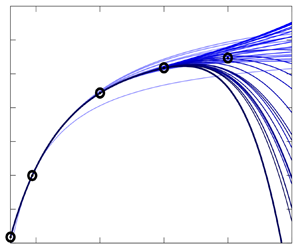
In figure 1, the predicted profiles of the velocity in the $x$-direction, $u$, and the velocity in the $y$-direction, $v$, are plotted at $\boldsymbol {x}=(2,0)$. The lightest (darkest) curve is the prediction of the order 1 (order 40) Taylor polynomial. The exact base flow, calculated with the method described in § 5.2, is depicted with black circles. It can be seen that for ${{Re}}=100$, the prediction is highly accurate, already at order $n\approx 7$ no difference to the true base flow is visible. The same goes for ${{Re}}=150$: at order $n\approx 12$, the difference with respect to the true base flow is negligible. At ${{Re}}=200$, however, the Taylor series diverges. The divergence can be seen on the profile of $v$. The prediction becomes worse at increasing order of the polynomials. The same behaviour can be observed in the whole computational domain. Further details on convergence will be discussed in § 5.3. Between ${{Re}}=150$ and ${{Re}}\approx 180$, the base flow is predicted less and less accurately, but the prediction improves with each order, until it reaches its convergence limit at ${{Re}}\approx 180$, where the prediction becomes worse when the order increases. Note that enforcing the transversal velocity $v$ to be zero at the symmetry axis does not change the convergence behaviour.

Figure 1. Taylor series expansion of the base flow along $a=1/{{Re}}$ conducted at $a_{0}=1/47$. Velocity profiles of the predicted base flows at $\boldsymbol {x}=(2,y)$ are plotted for Reynolds numbers 100 (a,b), 150 (c,d) and 200 (e,f). Directly calculated velocity profiles are plotted as black circles for comparison.

When expanding the leading eigenvalue into a Taylor polynomial, a similar convergence behaviour can be observed. In figure 2, the real and imaginary parts of the eigenvalue are plotted over the Reynolds number. Again, the lightest curve is the Taylor polynomial of order 1, the darkest of order 40. Directly calculated eigenvalues are plotted as black circles for comparison. Until ${{Re}}=150$, the eigenvalue can be predicted with the Taylor expansion. From then on, the prediction becomes less accurate, until the Taylor polynomials start to diverge. A difference between the convergence quality of the eigenvalue and the base flow cannot be observed. This suggests that at least in this case, the convergence behaviour of the eigenvalue is dictated by the convergence of the base flow. This is possible because the base flow coefficients $\boldsymbol {q}_{k}$ feed into the eigenvalue corrections (3.17).

Figure 2. Taylor series expansion of the eigenproblem along $a=1/{{Re}}$ conducted at $a_{0}=1/47$. The predicted real and imaginary parts of the eigenvalue are plotted over the Reynolds number for orders $n$ from 1 to 40. Directly calculated eigenvalues are plotted as black circles for comparison.

In figure 3, the computation time is plotted for the calculations of the various higher-order sensitivities. The calculation time is measured on one CPU and scaled by the time that is needed to solve one linear equation system with only real entries. This scaled CPU time is plotted on a logarithmic scale over the order of the Taylor polynomial. For the base flow sensitivities, computation time increases approximately exponentially. However, the calculations of base flow sensitivities up to order 40 is still faster than solving the nonlinear base flow equations (dashed line, calculated with a Newton solver in 7 iterations). For the eigenvalue sensitivities, a similar behaviour can be observed. These computation times are larger than those of the base flow sensitivities, because for each coefficient, a linear equation system with complex entries has to be solved, which has twice as many degrees of freedom. Again, calculating all coefficients until order 40 is faster than solving the eigenproblem directly for one eigenvalue and eigenvector (calculated as a shift-inverse problem with the Python package SciPy). For both eigenvalue and base flow coefficients, the computation time for approximately order 16 is twice as long as the time for the first solution of the linear equation system, i.e. the time to calculate the first-order coefficients. Thus, once the first-order coefficients are computed, higher orders follow at comparatively low computational costs.

Figure 3. Computation time for the higher-order sensitivities of the base flow and the eigenvalue, plotted over the order $n$. Dashed lines refer to the computation time for solving the nonlinear base flow equations (red) and the eigenproblem (blue). Note the logarithmic scale.

5.2. Subsequent computation of the base flow and its leading eigenvalue up to ${{Re}}=1000$

Even though the convergence of the base flow polynomial is finite, we can extend our prediction range by starting a new Taylor expansion at a new $a_{0}$ inside the convergence radius. Here, the following procedure was applied. Starting at ${{Re}}_{0}=30$, so that the expansion point is $a_0=\tfrac {1}{30}$, the base flow was expanded into a Taylor series until Taylor order 40. Then the Taylor approximation was evaluated at ${{Re}}_{0}=40$, thus yielding the base flow solution at a new Reynolds number inside the converged region. From there, a new Taylor series was expanded around $a_0=\tfrac {1}{40}$, and so on. At each step, the Reynolds number was increased by 10. By this method, the base flow was computed successfully until ${{Re}}=1000$. We note that the small step size used here and the high expansion order chosen may not have been strictly necessary to obtain an accurate solution of the NS equations as per (2.1), and to keep its residual (numerically) zero. However, a detailed investigation on the optimal performance of our algorithm in terms of step sizes and perturbation orders is beyond the scope of our work and will not be discussed here.

In figure 4, the calculated base flow is shown for Reynolds numbers 100, 500 and 1000. It can be seen that the gradients get sharper for higher Reynolds numbers. Accordingly, the width of the recirculation zone in the wake increases, while the length varies non-monotonically as the Reynolds number goes up. Near the symmetry axis, the back flow velocity increases significantly.

Figure 4. Base flow velocity components (a,c,e) $u(\boldsymbol {x})$ and (b,d,f) $v(\boldsymbol {x})$, for (a,b) ${{Re}}=100$, (c,d) ${{Re}}=500$, and (e,f) ${{Re}}=1000$. Computed with subsequent Taylor polynomial prediction, starting point was ${{Re}}=30$.

Next, the leading eigenvalue was traced until Reynolds number 1000. To do so, the eigenproblem was solved for several base flow solutions that were obtained with the method described previously, and the eigenvalue predictions conducted with the perturbation method were overlaid to construct a continuous curve. In figure 5(a), the real and imaginary parts of the eigenvalue versus ${{Re}}$ are shown. The dotted vertical lines indicate where the eigenproblem was solved. In the area between Reynolds numbers 200 and 420, the Reynolds number interval had to be decreased due to the poor convergence of the Taylor polynomials. This coincides with the area in which the convergence of the base flow is poor, thus indicating that the convergence of the eigenvalue is determined by the base flow in the whole Reynolds number range that was considered. Figure 5(b) shows part of the eigenvalue spectrum at ${{Re}}=1000$ (black dots) and the evolution of the leading eigenvalue with increasing Reynolds number. While the imaginary part decreases almost monotonically over the Reynolds number range, the real part first increases very quickly, and then increases and decreases again with a slowing rate. At ${{Re}}=1000$ it is still the leading eigenvalue of the entire spectrum. Figure 6 displays the eigenvectors of the traced eigenvalue for Reynolds numbers 100, 500 and 1000. Similar to the base flow itself, the gradients get sharper when the Reynolds number increases.

Figure 5. (a) Real and imaginary part of the traced eigenvalue over the Reynolds number. (b) Detail of the eigenvalue spectrum of the base flow at ${{Re}}=1000$. The traced eigenvalue is shown in varying colours for different Reynolds numbers.

Figure 6. Eigenvectors for (a,b) ${{Re}}=100$, (c,d) ${{Re}}=500$, and (e,f) ${{Re}}=1000$.

5.3. Remarks on convergence of the Taylor polynomials

In this subsection, we will take a closer look at the convergence behaviour of the Taylor polynomials that were computed in the previous subsection.

To quantify the convergence of the predicted base flow, we look at the $L_{2}$-norm of the NS base flow equations. We define

(5.1)\begin{equation} L_{2}(n,a,a_{0}):=\frac{1}{\sqrt{A}}\left\Vert \boldsymbol{N}\left(\boldsymbol{q}^{(n)}(a), a\right)\right\Vert _{2}=\frac{1}{\sqrt{A}}\left\langle \boldsymbol{N}\left(\boldsymbol{q}^{(n)}(a), a\right)\!,\boldsymbol{N}\left(\boldsymbol{q}^{(n)}(a), a\right)\right\rangle ^{{1}/{2}}\end{equation}

with the surface area of the computational domain $A$, and equations (2.1), (2.3) and (2.4). It holds that

(5.2)\begin{equation} \lim_{n\rightarrow \infty} L_{2}(n,a,a_{0}) = 0 \end{equation}

if

(5.3)\begin{equation} |\epsilon|\equiv|a-a_{0}|< r \end{equation}

for a certain convergence radius $r$. In a looser sense, one may state that the series truncated at a finite order $n$ provides a good approximation to the actual solution if $L_{2}(n,a,a_{0}) < \delta$, where $\delta$ is a small error threshold. This means that the NS base flow equation should be (approximately) fulfilled for the predicted base flow in a certain region around $a_{0}$, and the smaller $L_{2}$, the better the prediction.

First, we look at the convergence of the base flow prediction for the parameter $a={{Re}}$. The parameter-specific details of the calculations can be found in Appendix A. Figure 7(a) shows the $L_{2}$-norm of the NS equations for the predicted base flows when expanded around $a_{0}={{Re}}_{0}=30$. The lightest curve depicts the first-order prediction, $n=1$, and the darkest curve depicts the prediction of order $40$. The norm is shown on a logarithmic scale.

Figure 7. Taylor expansion of the base flow; the $L_{2}$-norm of the NS equations is plotted over the expansion parameter and serves as an error measurement. (a) Expansion parameter $a={{Re}}$, conducted at $a_{0}=30$, diverges for $a<0$ and $a>2a_{0}=60$ (vertical dashed line). (b) Expansion parameter $a=1/{{Re}}$, conducted at $a_{0}=1/10$, diverges for $a<0$ and $a>2a_{0}=1/5$. Note the logarithmic scale of the $L_{2}$-norm. Mesh A (AF).

It can be seen that the Taylor polynomial converges if $|a-a_{0}|< a_{0}$, and diverges otherwise. This behaviour can be explained by the manner in which the Reynolds number appears in the NS equations. Just like the Taylor series for the function $f(x)=1/x$, the NS equations have a singularity at ${{Re}}=0$. This singularity limits the convergence of any power series related to the equations, and the base flow convergence radius is therefore $a_{0}={{Re}}_{0}$. Therefore, the base flow cannot be predicted for ${{Re}}>2{{Re}}_{0}$ if the chosen parameter is the Reynolds number itself, because the related series diverges.

Using the parameter $a=1/{{Re}}$ for the perturbation expansion yields a qualitatively similar but quantitatively different convergence result. In figure 7(b), the $L_{2}$-norm of the NS equations is depicted for the predicted base flows, when expanded around $a_{0}=1/{{Re}}_{0}=1/10$. It is known that the NS equations have a singular point at $a=0$, i.e. ${{Re}}=\infty$. This divergence is due to the fact that with no viscous term, the NS equations turn into the Euler equations, which need a different boundary condition at the cylinder wall. Thus also in this case, $a_{0}$ defines an upper limit for the convergence radius. Nonetheless, there may exist other singularities that would reduce the radius of convergence further.

While the convergence behaviour when expanding around small Reynolds numbers is defined by the singular point at ${{Re}}=0$, the behaviour when starting at higher Reynolds numbers is not described as easily. In figure 8, the convergence behaviour of the base flow Taylor polynomials is depicted for the parameter $a=1/{{Re}}$ and $a_{0}=1/47$. The $L_{2}$-norm of the NS equations against the $a$ parameter is plotted in figure 8(a). For convenience, the same results are shown in figure 8(b) by using the parameter $1/a = {{Re}}$ on the horizontal axis. In figure 8(a), it can be seen that the Taylor polynomials converge in a symmetric region around the expansion point. This symmetry is lost in figure 8(b), because the scaling $1/a$ stretches the results in different ways for small/large Reynolds numbers. It can be seen that a good approximation is obtained up to ${{Re}}\approx 180$. We remark that if we had chosen to use $a={{Re}}$ as the expansion parameter, then an upper limit for the convergence radius would be given by ${{Re}}_0 = 47$, because of the singularity of the equations at ${{Re}}=0$. Thus the result would surely diverge for ${{Re}}>94$. This comparison shows that the choice of the expansion parameter has an influence on the largest achievable Reynolds number, and that in the case considered here, using the parameter $a=1/{{Re}}$ allows us to obtain accurate results for larger values of ${{Re}}$.

Figure 8. Taylor series expansion of the base flow along $a=1/{{Re}}$; a norm of the NS equations is plotted over (a) the inverse of the Reynolds number, and (b) the Reynolds number itself. Starting point is $a_{0}=1/47$. Mesh A (AF).

6. Stabilization through a small control cylinder

A well-known control scenario of the so-far depicted two-dimensional cylinder flow instability is a small control cylinder, which is placed inside the domain. In the vortex shedding flow regime, it stabilizes the flow at certain positions for relatively low Reynolds numbers. With the help of sensitivity maps, those stabilizing regions can be estimated. These maps were first calculated by Marquet et al. (Reference Marquet, Sipp and Jacquin2008), who calculated the first-order sensitivity of the leading eigenvalue. They were extended to second order by Boujo (Reference Boujo2021), who could improve qualitative agreement with experimental results by Strykowski & Sreenivasan (Reference Strykowski and Sreenivasan1990) significantly. They all used a simplified model for the small control cylinder, which consists of estimating the drag force acting back on the flow as a steady forcing.

In this section, we extend the calculation of these sensitivity maps to higher orders for Reynolds numbers 60, 70, 80 and 90, and a control cylinder diameter $d=0.1$. We compare Taylor predictions up to order 10 with low-order predictions, as well as with full eigenvalue calculations, for which the small control cylinder is built directly into the grid, and no-slip Dirichlet boundary conditions are imposed.

6.1. Model equations

Following Hill (Reference Hill1992), Marquet et al. (Reference Marquet, Sipp and Jacquin2008) and Boujo (Reference Boujo2021), we model the small control cylinder of diameter $d$ located in $\boldsymbol {x}_c$ as a steady forcing acting on the base flow. Its magnitude is defined by the drag force that would act on the small cylinder in uniform flow, and the forcing is distributed along a two-dimensional Gaussian function. In particular, we use the same drag coefficient as Boujo (Reference Boujo2021), but add a model for the variance of the Gaussian function, to make the predictions more accurate and to avoid convergence issues of the Taylor polynomial. The forcing is thus defined as

(6.1)\begin{equation} \boldsymbol{F}(\boldsymbol{x}_c,d)=\tfrac{1}{2}\,d\,C_{d}(\boldsymbol{x}_{c})\,\Vert\boldsymbol{u}_{0}(\boldsymbol{x}_{c})\Vert\,\boldsymbol{u}_{0}(\boldsymbol{x}_{c})\, \boldsymbol{\chi}(\boldsymbol{x}-\boldsymbol{x}_{c},\sigma^{2}), \end{equation}

with the local Reynolds number

(6.2)\begin{equation} {{Re}}_{d}(\boldsymbol{x}_{c})\equiv\frac{d\,\Vert\boldsymbol{u}_{0}(\boldsymbol{x}_{c})\Vert}{\nu}, \end{equation}

and the drag coefficient $C_{d}(\boldsymbol {x}_{c})=0.8558+10.05({{Re}}_{d}(\boldsymbol {x}_{c}))^{-0.7004}$. Pivotal is the velocity of the unperturbed base flow $\boldsymbol {u}_0$ at the centre $\boldsymbol {x}_c$ of the small cylinder. Here, $\boldsymbol {\chi }(\boldsymbol {x}-\boldsymbol {x}_{c},\sigma ^{2})$ is a two-dimensional Gaussian function that is distributed symmetrically around $\boldsymbol {x}_{c}$ with variance $\sigma ^{2}$. We add a linear dependence of the standard deviation with regard to the magnitude of the forcing to improve results in comparison to the small control cylinder incorporated directly into the grid. The standard deviation is thus

(6.3)\begin{equation} \sigma = \max\left[\sigma_{min}, d\left(\tfrac{1}{2}\,C_d\,\Vert\boldsymbol{u}_0(\boldsymbol{x}_c)\Vert^2-1 \right)\right]\!, \end{equation}

where $\sigma _{{min}}$ ensures that the Gaussian function can be depicted accurately enough with the given grid resolution. Here, we choose $\sigma _{{min}}=0.025$ in combination with grid B (see table 1). We recall that only dimensionless variables appear in (6.3), and that the velocity and diameter of the small control cylinder has to be made dimensionless for (6.3) to hold.

In the following, we consider a small control cylinder of diameter $d=0.1$. The expansion parameter $a$ is chosen to be the amplitude of the steady forcing such that the base flow equations become

(6.4) \begin{equation} \boldsymbol{N}(\boldsymbol{q},a)=\left(\begin{array}{@{}c@{}} (\boldsymbol{u}\boldsymbol{\cdot}\boldsymbol{\nabla})\boldsymbol{u}+\boldsymbol{\nabla} p-\dfrac{1}{Re}\,\nabla^{2}\boldsymbol{u}\\ \boldsymbol{\nabla}\boldsymbol{\cdot}\boldsymbol{u} \end{array}\right)+a\left(\begin{array}{@{}c@{}}\boldsymbol{F}\\0\end{array}\right)= \boldsymbol 0 . \end{equation}

Thus $a$ is a scalar factor that is expanded from $a_{0}=0$. It is related to the diameter of the small control cylinder in the above model via

(6.5)\begin{equation} a(d,\boldsymbol{x}_{c})\equiv\frac{d\,C_{d}(\boldsymbol{x}_{c})}{0.1\,C_{0.1}(\boldsymbol{x}_{c})} \end{equation}

such that $a(d=0.1,\boldsymbol {x}_{c})=1$.

The first-order partial derivative of the steady NS equations is

(6.6)\begin{equation} \boldsymbol{N}_{a}=\left(\begin{array}{@{}c@{}} \boldsymbol F\\0 \end{array}\right), \end{equation}

and (2.17) simplifies to

(6.7)\begin{equation} \boldsymbol{N}_{\boldsymbol{q}}\boldsymbol{q}_{k}=\left\{ \begin{array}{@{}ll} -\left(\begin{array}{@{}c@{}} \boldsymbol F\\0 \end{array}\right)\!, & \text{for}\ k=1,\\ -\dfrac{1}{2}\displaystyle\sum_{i=1}^{k-1}\left(\begin{array}{@{}c@{}} k\\ i \end{array}\right)\boldsymbol{q}_{i}^{\rm T}\boldsymbol{N}_{\boldsymbol{qq}}\boldsymbol{q}_{k-i}, & \text{for}\ k>1 . \end{array}\right. \end{equation}

The coefficients for the Taylor expansion of the linear operator, needed in the prediction of the eigenvalue, are (see (3.12))

(6.8)\begin{equation} \boldsymbol{\mathsf{L}}{}_{k}\boldsymbol{q}_{j}=\boldsymbol{q}_{k}^{\rm T} \boldsymbol{N}_{\boldsymbol{qq}}\boldsymbol{q}_{j}. \end{equation}

6.2. Higher-order sensitivity maps of the control cylinder

The higher-order sensitivity maps are calculated by computing the Taylor coefficients of the model described above up to order 10 at 0.1 increments in the $x$- and $y$-directions. Thus for each Reynolds number, a total of 496 control cylinder positions were computed. As discussed before, the preconditioning of the linear equation systems can be exploited for the whole map once the undisturbed base flow and eigenproblem are given, making the computation very efficient. Computing one map until Taylor order 10, with the implementation described here, cost the equivalent of approximately 30 base flow computations and 26 eigenvalue computations (on one CPU, non-parallel). We recall that with this method, the base flows and leading eigenvalues were predicted not only for 496 discrete cylinder positions, but also for a continuous range of control cylinder diameters within the validity of the used model. Also, as will be seen later, calculating the coefficients up to order 10 is not needed for sufficient convergence at most positions. Because the computation time increases exponentially with every order (see figure 3), taking into account the convergence behaviour would reduce the computation time even further.

In figure 9 the regions in which a small control cylinder stabilizes the flow are drawn for Reynolds numbers 60, 70, 80 and 90, and Taylor polynomial orders from 1 to 10. The drawn lines are B-spline interpolations of the calculated grid data. For comparison, the eigenproblem was also solved with the small control cylinder inserted directly into the grid, with finer grid resolution in the vicinity of the wall, and Dirichlet boundary conditions. To identify the value at which the growth rate of the eigenvalue is zero, for each point, two control cylinder positions were calculated at distance 0.06, and the resulting position was computed by first-order interpolation. When necessary, one or two additional positions were calculated. This procedure was possible because the approximate coordinates of the resulting points were already known from the high-order perturbation expansion results.

Figure 9. Predicted stabilizing regions until order 10, using a steady forcing to model the small control cylinder with diameter 0.1, for Reynolds numbers 60, 70, 80 and 90. Black circles are values calculated from incorporating the small control cylinder directly into the grid. Small crosses are experimental data from Strykowski & Sreenivasan (Reference Strykowski and Sreenivasan1990). Note that the minimum visible order varies: for ${{Re}}=60$, order 1 already depicts a stabilizing region; for ${{Re}}=70$, order 2 is needed; for ${{Re}}=80$, order 3; and for ${{Re}}=90$, order 5 (the lighter the contours, the higher the expansion order).

As can be seen in figure 9, the higher-order Taylor predictions of the steady forcing model are generally in very good agreement with the values from a direct computation using the embedded control cylinder. The deviation for ${{Re}}=60$ and 70, visible at the streamwise end of the stabilizing region, stems from the grid resolution: with a finer grid, a smaller $\sigma _{min}$ in (6.3) would have been possible. This was verified by performing calculations on the finer BF grid; see table 1. Since in these regions the respective base flow shows a comparatively low absolute velocity and thus a comparatively low forcing value is needed, the borders of the stability regions would have been more accurate with a steeper Gaussian function. At higher Reynolds numbers, this problem does not occur.

Note that the higher the Reynolds number, the higher the expansion order needed to depict the stable regions accurately. While for ${{Re}}=60$ the second-order prediction is already fairly accurate, for ${{Re}}=70$ it is vital for detecting a stabilizing area at all, since the first-order expansion predicts no stabilization in the whole computational domain. These results compare well to the second-order results from Boujo (Reference Boujo2021). Subsequently, for ${{Re}}=80$, expansion order 3 is needed to detect the stabilizing area, and for ${{Re}}=90$, the region appears only for orders $n\ge 5$. Experimental data from Strykowski & Sreenivasan (Reference Strykowski and Sreenivasan1990) for Reynolds numbers 60 and 70 have been added for completeness. They are slightly more unstable than the numerical data. The authors themselves discuss that, due to the experimental set-up, three-dimensional effects occur, and thus the two-dimensionality assumption is not completely accurate. In this light, the results compare well to the numerical data depicted here.

7. Conclusion and outlook

In this study, base flow and eigenvalue sensitivities of arbitrary order with respect to a generic scalar parameter were derived for the incompressible Navier–Stokes (NS) equations. With these, we showed how the base flow and eigenvalues of the linear operator of the NS equations can be expanded in Taylor polynomials. Given the structure of the incompressible NS equations, the calculation of the higher-order sensitivities prove to be very computationally efficient. For each higher-order coefficient, a linear equation system has to be solved, whose left-hand side contains the same linear operator for all orders. Thus once the first-order sensitivity is found and a preconditioner has been computed, each following higher order can be calculated very efficiently. The derived equations were applied on the two-dimensional cylinder base flow, first by using the inverse of the Reynolds number as parameter, and later to calculate sensitivity maps of higher order for the case of a small control cylinder inserted into the domain.

For ${{Re}}=47$, i.e. at the onset of flapping, a Taylor expansion of the base flow and of the leading eigenvalue was conducted until order 40. The prediction in these two cases was accurate until approximately ${{Re}}=150$, after which inaccuracies occurred, even for high orders. The Taylor polynomials were shown to diverge for ${{Re}}>180$, due to the finite radius of convergence of the computed power series. As the radius of convergence limits the prediction horizon when expanding the cylinder base flow into a Taylor polynomial around the Reynolds number, a procedure is proposed to extend the predictions further by performing another expansion around a new parameter value that lies within the convergence area. Following this procedure, the cylinder base flow was calculated efficiently up to ${{Re}}=1000$. The leading eigenvalue was also traced for the whole Reynolds number range by solving the eigenproblem at distinctive Reynolds numbers and predicting the eigenvalues in between by Taylor expansions. No additional symmetry condition had to be imposed, and the base flow could be computed regardless of the kind or number of unstable eigenmodes.

The convergence behaviour of the Taylor polynomials was investigated further and found to be dependent on several quantities. First, the choice of parameter was shown to be important. For the Reynolds number as scalar parameter, when expanding around small values of ${{Re}}$, the maximum convergence radius is the Reynolds number itself, because the NS equations have a singularity at ${{Re}}=0$. The same holds for the inverse of the Reynolds number, since the equations are singular also at ${{Re}}=\infty$. Second, we showed that the radius of convergence is dependent on the actual value of the parameter around which the Taylor polynomials are expanded. One possible explanation for this behaviour comes from singular points for complex values of the Reynolds number, which then dictate the convergence behaviour for real-valued expansion parameters. In the case considered, the convergence radius of the eigenvalue polynomials is approximately the same as for the respective base flow, suggesting that for the Reynolds number range that is investigated in this work, the convergence behaviour of the eigenvalue expansion is determined by the convergence behaviour of the base flow expansion.

Finally, we have demonstrated the use of the high-order perturbation method on a passive flow control application; we have calculated sensitivity maps of higher order to determine the regions in the domain, where a small control cylinder stabilizes the flow for Reynolds numbers 60–90. We modelled the control cylinder with a Gaussian-distributed, steady forcing. The agreement with numerical data, for which the control cylinder was incorporated directly into the grid, was found to be very good. Depending on the Reynolds number, Taylor orders 3–8 are necessary to draw the areas with sufficient precision. Because the base flow was calculated only once, and because for each order only one equation system had to be solved, which was already preconditioned, these calculations prove to be computationally efficient. As before, once the preconditioner is computed, it can be exploited for the whole computational domain and all Taylor orders.

The work presented here has the potential to be extended and applied to other scenarios. For instance, the method to calculate unstable base flows could be improved to make it computationally more efficient, by answering the questions of the optimal expansion order and the optimal step size. Furthermore, there is still scope for understanding the reasons that limit the convergence of the constructed series. While for first-order computations a large number of parameters is possible, at higher orders the number of parameters is limited. Nevertheless, the method presented here can be extended to a finite number of parameters and relatively low expansion orders. A last area of use for the demonstrated method is the RANS equations, by including the higher-order derivatives of the turbulence model. With the method presented here, a continuous range of RANS solutions along a scalar parameter could be computed.

Funding

The funding of the Deutsche Forschungsgemeinschaft (DFG – German Research Foundation) under project no. 441269395 is acknowledged. This work was also funded by a fellowship of the Berlin International Graduate School in Model and Simulation based Research (BIMoS).

Declaration of interests

The authors report no conflict of interest.

Appendix A. The parameter $a={{Re}}$

Consider the parameter $a$ being the Reynolds number ${{Re}}$. Then (2.3) reads for the incompressible NS equations

(A1)\begin{equation} \boldsymbol{N}(\boldsymbol{q}(a),a)=\left(\begin{array}{@{}c@{}} (\boldsymbol{u}(a)\boldsymbol{\cdot}\boldsymbol{\nabla})\,\boldsymbol{u}(a)+\boldsymbol{\nabla} p(a)-\dfrac{1}{a}\,\nabla^{2}\boldsymbol{u}(a)\\ \boldsymbol{\nabla}\boldsymbol{\cdot}\boldsymbol{u}(a) \end{array}\right)=0 . \end{equation}

Only four types of terms are needed for the calculation of $\boldsymbol {q}_{k}$ and $\boldsymbol{\mathsf{L}}_{k}$, because every partial derivative with respect to $a$ vanishes if it is greater than first order in $\boldsymbol {q}$, i.e.

(A2)\begin{equation} \boldsymbol{N}_{\boldsymbol{qq}a}=0=\boldsymbol{N}_{\boldsymbol{qq}aa}=\boldsymbol{N}_{\boldsymbol{qq}aaa}=\cdots. \end{equation}

With this simplification, (2.17) becomes

(A3)\begin{equation} \boldsymbol{N}_{\boldsymbol{q}}\boldsymbol{q}_{k}=-\sum_{i=1}^{k-1}\left(\begin{array}{@{}c@{}} k\\ i \end{array}\right)\left[\frac{1}{2}\,\boldsymbol{q}_{i}^{\rm T}\boldsymbol{N}_{\boldsymbol{qq}}\boldsymbol{q}_{k-i}+\boldsymbol{N}_{\boldsymbol{q}a^{i}}\boldsymbol{q}_{k-i}\right]-\boldsymbol{N}_{a^{k}}, \end{equation}

and (3.12) simplifies to

(A4)\begin{equation} \boldsymbol{\mathsf{L}}_{k}\boldsymbol{q}_{i}=\boldsymbol{q}_{k}^{\rm T}\boldsymbol{N}_{\boldsymbol{qq}}\boldsymbol{q}_{i}+\boldsymbol{N}_{\boldsymbol{q}a^{k}}\boldsymbol{q}_{i} . \end{equation}

The terms appearing are

(A5)\begin{gather} \boldsymbol{N}_{\boldsymbol{q}}\boldsymbol{q}_{k}=\left(\begin{array}{@{}c@{}} (\boldsymbol{u}_{0}\boldsymbol{\cdot}\boldsymbol{\nabla})\boldsymbol{u}_{k}+(\boldsymbol{u}_{k}\boldsymbol{\cdot}\boldsymbol{\nabla})\boldsymbol{u}_{0}+\boldsymbol{\nabla} p_{k}-\dfrac{1}{a_{0}}\,\nabla^{2}\boldsymbol{u}_{k}\\ \boldsymbol{\nabla}\boldsymbol{\cdot}\boldsymbol{u}_{k} \end{array}\right)\!, \end{gather}
(A6)\begin{gather} \boldsymbol{q}_{i}^{\rm T}\boldsymbol{N}_{\boldsymbol{qq}}\boldsymbol{q}_{j}=\left(\begin{array}{@{}c@{}} (\boldsymbol{u}_{i}\boldsymbol{\cdot}\boldsymbol{\nabla})\boldsymbol{u}_{j}+(\boldsymbol{u}_{j}\boldsymbol{\cdot}\boldsymbol{\nabla})\boldsymbol{u}_{i}\\[2pt] 0 \end{array}\right)\!, \end{gather}
(A7)\begin{gather} \boldsymbol{N}_{a^{k}}=\left(\begin{array}{@{}c@{}} \dfrac{(-1)^{k}\,k!}{a_{0}^{k+1}}\,\nabla^{2}\boldsymbol{u}_{0}\\ 0 \end{array}\right)\!, \end{gather}
(A8)\begin{gather} \boldsymbol{N}_{\boldsymbol{q}a^{k}}\boldsymbol{q}_{i}=\left(\begin{array}{@{}c@{}} \dfrac{(-1)^{k}\,k!}{a_{0}^{k+1}}\,\nabla^{2}\boldsymbol{u}_{i}\\ 0 \end{array}\right) . \end{gather}

Appendix B. Further remarks on the convergence behaviour when expanding along the Reynolds number

Here, we will take a (very short) closer look at the relation of the convergence quality to $a_{0}$. To do so, we define a maximal Reynolds number until which the $L_2$-norm of the NS equations (5.1) is smaller than $10^{-10}$,

(B1)\begin{equation} {{Re}}_{{max}}:=\dfrac{1}{a_{{0}}-\epsilon},\quad\left\Vert \boldsymbol{N}\left(\boldsymbol{q}^{(n)}(a_{0}-\epsilon),a_{0}-\epsilon\right)\right\Vert _{2}\approx10^{-10},\quad\epsilon>0, \end{equation}

depending on the Reynolds number ${{Re}}_{0}:={1}/{a_{0}}$ from which the Taylor polynomial was expanded. Figure 10 shows the difference of ${{Re}}_{{max}}$ and ${{Re}}_{0}$ plotted over ${{Re}}_{0}$ for orders 10, 20, 30 and 40. It can be seen that the quality of the prediction improves with the order, as expected. The prediction horizon has a noticeable dent between approximately ${{Re}}_{0}=100$ and ${{Re}}_{0}=450$, where the Taylor polynomial can reproduce the correct base flow only in a very small Reynolds number range. Also, the differences between the respective orders are small in this region. This shows that the convergence quality of the Taylor polynomials can diverge significantly for different starting points $a_{0}$.

Figure 10. Plots of (${{Re}}_{{max}}-{{Re}}_{0}$) for $n=10,20,30,40$ plotted over ${{Re}}_{0}$.

References

Akervik, E., Brandt, L., Henningson, D.S., Hoepffner, J., Marxen, O. & Schlatter, P. 2006 Steady solutions of the Navier–Stokes equations by selective frequency damping. Phys. Fluids 18, 068102.CrossRefGoogle Scholar
Alnæs, M.S., Blechta, J., Hake, J., Johansson, A., Kehlet, B., Logg, A., Richardson, C., Ring, J., Rognes, M.E. & Wells, G.N. 2015 The FEniCS project version 1.5. Arch. Numer. Softw. 3 (100), 923.Google Scholar
Baysal, O. & Eleshaky, M.E. 1992 Aerodynamic design optimization using sensitivity analysis and computational fluid dynamics. AIAA J. 30 (3), 718725.CrossRefGoogle Scholar
Bender, C.M. & Orszag, S.A. 1999 Advanced Mathematical Methods for Scientists and Engineers. Springer.CrossRefGoogle Scholar
Boujo, E. 2021 Second-order adjoint-based sensitivity for hydrodynamic stability and control. J. Fluid Mech. 920, A12.CrossRefGoogle Scholar
Boujo, E., Fani, A. & Gallaire, F. 2015 Second-order sensitivity of parallel shear flows and optimal spanwise-periodic flow modifications. J. Fluid Mech. 782, 491514.CrossRefGoogle Scholar
Boujo, E., Fani, A. & Gallaire, F. 2019 Second-order sensitivity in the cylinder wake: optimal spanwise-periodic wall actuation and wall deformation. Phys. Rev. Fluids 4, 053901.CrossRefGoogle Scholar
Boyd, J.P. 1999 The Devil's invention: asymptotic, superasymptotic and hyperasymptotic series. Acta Appl. Math. 56, 198.CrossRefGoogle Scholar
Casacuberta, J., Groot, K.J., Tol, H.J. & Hickel, S. 2018 Effectivity and efficiency of selective frequency damping for the computation of unstable steady-state solutions. J. Comput. Phys. 375, 481497.CrossRefGoogle Scholar
Del Guercio, G., Cossu, C. & Pujals, G. 2014 Optimal perturbations of non-parallel wakes and their stabilizing effect on the global instability. Phys. Fluids 26, 024110.CrossRefGoogle Scholar
Giannetti, F., Camarri, S. & Citro, V. 2019 Sensitivity analysis and passive control of the secondary instability in the wake of a cylinder. J. Fluid Mech. 864, 4572.CrossRefGoogle Scholar
Giannetti, F. & Luchini, P. 2007 Structural sensitivity of the first instability of the cylinder wake. J. Fluid Mech. 581, 167197.CrossRefGoogle Scholar
Hill, D.C. 1992 A theoretical approach for analyzing the restabilization of wakes. In 30th Aerospace Sciences Meeting and Exhibit. AIAA. https://doi.org/10.2514/6.1992-67.CrossRefGoogle Scholar
Hwang, Y., Kim, J. & Choi, H. 2013 Stabilization of absolute instability in spanwise wavy two-dimensional wakes. J. Fluid Mech. 727, 346378.CrossRefGoogle Scholar
Jordi, B.E., Cotter, C.J. & Sherwin, S.J. 2015 An adaptive selective frequency damping method. Phys. Fluids 27, 094104.CrossRefGoogle Scholar
Kaiser, T.L., Demange, S., Müller, J.S., Knechtel, S. & Oberleithner, K. 2023 b FELiCS: A Versatile Linearized Solver Addressing Dynamics in Multi-Physics Flows. AIAA AVIATION 2023 Forum. p. 3434.Google Scholar
Kaiser, T.L. & Oberleithner, K. 2021 A global linearized framework for modelling shear dispersion and turbulent diffusion of passive scalar fluctuations. J. Fluid Mech. 915, A111.CrossRefGoogle Scholar
Kaiser, T.L., Varillon, G., Polifke, W., Zhang, F., Zirwes, T., Bockhorn, H. & Oberleithner, K. 2023 a Modelling the response of a turbulent jet flame to acoustic forcing in a linearized framework using an active flame approach. Combust. Flame 253, 112778.CrossRefGoogle Scholar
Kato, T. 1980 Perturbation Theory for Linear Operators. Springer.Google Scholar
Lancaster, P., Markus, A.S. & Zhou, F. 2003 Perturbation theory for analytic matrix functions: the semisimple case. SIAM J. Matrix Anal. Appl. 25 (3), 606626.CrossRefGoogle Scholar
Luchini, P. & Bottaro, A. 2014 a Adjoint equations in stability analysis. Annu. Rev. Fluid Mech. 46, 493517.CrossRefGoogle Scholar
Luchini, P. & Bottaro, A. 2014 b An introduction to adjoint problems. Annu. Rev. Fluid Mech. 46, 493517, Supplemental Material.CrossRefGoogle Scholar
Marquet, O., Sipp, D. & Jacquin, L. 2008 Sensitivity analysis and passive control of cylinder flow. J. Fluid Mech. 615, 221252.CrossRefGoogle Scholar
Mensah, G.A., Orchini, A. & Moeck, J.P. 2020 Perturbation theory of nonlinear, non-self-adjoint eigenvalue problems: simple eigenvalues. J. Sound Vib. 473, 115200.CrossRefGoogle Scholar
Oden, J.T. 1979 Applied Functional Analysis. Prentice Hall.Google Scholar
Orchini, A., Magri, L., Silva, C.F., Mensah, G.A. & Moeck, J.P. 2020 Degenerate perturbation theory in thermoacoustics: high-order sensitivities and exceptional points. J. Fluid Mech. 903, A37.CrossRefGoogle Scholar
Seyranian, A.P., Kirillov, O.N. & Mailybaev, A.A. 2005 Coupling of eigenvalues of complex matrices at diabolic and exceptional points. J. Phys. A: Math. Gen. 38 (8), 17231740.CrossRefGoogle Scholar
Strykowski, P.J. & Sreenivasan, K.R. 1990 On the formation and suppression of vortex ‘shedding’ at low Reynolds numbers. J. Fluid Mech. 218, 71107.CrossRefGoogle Scholar
Tammisola, O. 2017 Optimal wavy surface to suppress vortex shedding using second-order sensitivity to shape changes. Eur. J. Mech. (B/Fluids) 62, 139148.CrossRefGoogle Scholar
Tammisola, O., Giannetti, F., Citro, V. & Juniper, M.P. 2014 Second-order perturbation of global modes and implications for spanwise wavy actuation. J. Fluid Mech. 755, 314335.CrossRefGoogle Scholar
Van Dyke, M. 1975 Perturbation Methods in Fluid Mechanics. Parabolic Press.Google Scholar
Figure 0

Table 1. Meshes. All meshes are elliptical. The ellipse extensions refer to the inner regions with higher grid resolution ($\Delta x_{max}$ in the columns before).

Figure 1

Figure 1. Taylor series expansion of the base flow along $a=1/{{Re}}$ conducted at $a_{0}=1/47$. Velocity profiles of the predicted base flows at $\boldsymbol {x}=(2,y)$ are plotted for Reynolds numbers 100 (a,b), 150 (c,d) and 200 (e,f). Directly calculated velocity profiles are plotted as black circles for comparison.

Figure 2

Figure 2. Taylor series expansion of the eigenproblem along $a=1/{{Re}}$ conducted at $a_{0}=1/47$. The predicted real and imaginary parts of the eigenvalue are plotted over the Reynolds number for orders $n$ from 1 to 40. Directly calculated eigenvalues are plotted as black circles for comparison.

Figure 3

Figure 3. Computation time for the higher-order sensitivities of the base flow and the eigenvalue, plotted over the order $n$. Dashed lines refer to the computation time for solving the nonlinear base flow equations (red) and the eigenproblem (blue). Note the logarithmic scale.

Figure 4

Figure 4. Base flow velocity components (a,c,e) $u(\boldsymbol {x})$ and (b,d,f) $v(\boldsymbol {x})$, for (a,b) ${{Re}}=100$, (c,d) ${{Re}}=500$, and (e,f) ${{Re}}=1000$. Computed with subsequent Taylor polynomial prediction, starting point was ${{Re}}=30$.

Figure 5

Figure 5. (a) Real and imaginary part of the traced eigenvalue over the Reynolds number. (b) Detail of the eigenvalue spectrum of the base flow at ${{Re}}=1000$. The traced eigenvalue is shown in varying colours for different Reynolds numbers.

Figure 6

Figure 6. Eigenvectors for (a,b) ${{Re}}=100$, (c,d) ${{Re}}=500$, and (e,f) ${{Re}}=1000$.

Figure 7

Figure 7. Taylor expansion of the base flow; the $L_{2}$-norm of the NS equations is plotted over the expansion parameter and serves as an error measurement. (a) Expansion parameter $a={{Re}}$, conducted at $a_{0}=30$, diverges for $a<0$ and $a>2a_{0}=60$ (vertical dashed line). (b) Expansion parameter $a=1/{{Re}}$, conducted at $a_{0}=1/10$, diverges for $a<0$ and $a>2a_{0}=1/5$. Note the logarithmic scale of the $L_{2}$-norm. Mesh A (AF).

Figure 8

Figure 8. Taylor series expansion of the base flow along $a=1/{{Re}}$; a norm of the NS equations is plotted over (a) the inverse of the Reynolds number, and (b) the Reynolds number itself. Starting point is $a_{0}=1/47$. Mesh A (AF).

Figure 9

Figure 9. Predicted stabilizing regions until order 10, using a steady forcing to model the small control cylinder with diameter 0.1, for Reynolds numbers 60, 70, 80 and 90. Black circles are values calculated from incorporating the small control cylinder directly into the grid. Small crosses are experimental data from Strykowski & Sreenivasan (1990). Note that the minimum visible order varies: for ${{Re}}=60$, order 1 already depicts a stabilizing region; for ${{Re}}=70$, order 2 is needed; for ${{Re}}=80$, order 3; and for ${{Re}}=90$, order 5 (the lighter the contours, the higher the expansion order).

Figure 10

Figure 10. Plots of (${{Re}}_{{max}}-{{Re}}_{0}$) for $n=10,20,30,40$ plotted over ${{Re}}_{0}$.