


1. Introduction
Drop-off and curbside recycling are two of the widely used recycling programs in the United States. Drop-off recycling allows individuals to collect their recyclables and drop them off at a designated site. Curbside recycling allows individuals to leave recyclables by their curbside so that waste and recycling pickup service providers in the area can pick them up. There have been a wide range of studies in the literature that examined socioeconomic aspects of recycling (e.g. comparison of costs between waste disposal and recycling (Bohm et al., Reference Bohm, Folz, Kinnaman and Podolsky2010); comparison between revenue from recycled materials and cost of collection (Lavee, Reference Lavee2007); effects of local laws on household waste disposal and recycling behaviors (Kinnaman & Fullerton, Reference Kinnaman and Fullerton2000); determinants of recycling rates (Saphores et al., Reference Saphores, Nixon, Ogunseitan and Shapiro2006; Sidique et al., Reference Sidique, Joshi and Lupi2010); demographic determinants of recycling participation (Ferrara & Missios, Reference Ferrara and Missios2005; Viscusi et al., Reference Viscusi, Huber and Bell2011); socially optimal recycling rate based on costs to households and benefits based on life-cycle analysis (Kinnaman et al., Reference Kinnaman, Shinkuma and Yamamoto2014); and effects of pay-as-you-throw (“fine” for generating waste) on recycling participation (Fullerton & Kinnaman, Reference Fullerton and Kinnaman2017).
The economic value of recycling, particularly willingness-to-pay for curbside pickup, has also been studied in the literature, using stated preference methods (e.g. Aadland & Caplan, Reference Aadland and Caplan1999, Reference Aadland and Caplan2003, Reference Aadland and Caplan2006; Blaine et al., Reference Blaine, Lichtkoppler, Jones and Zondag2005; Koford et al., Reference Koford, Blomquist, Hardesty, Troske, Hughes-Morgan and Morgan2012; Challcharoenwattana & Pharino, Reference Challcharoenwattana and Pharino2016; Hwang, Reference Hwang2024). Stated preference methods refer to a type of non-market valuation technique used in the field of economics to measure the economic value of goods and services that are not traded in the market, such as environmental amenities and public programs, based on hypothetical choices made in surveys. Revealed preference methods, on the other hand, refer to a type of non-market valuation technique that measures the economic value of similar goods and services based on actual choices and behaviors rather than hypothetical choices. Sidique et al. (Reference Sidique, Lupi and Joshi2013), for example, estimated the demand for recycling drop-off, using an application of the travel cost method (TCM), which is a type of revealed preference method. More specifically, they used the random utility model to measure the implicit prices of drop-off site characteristics, such as hours of operation, number of recyclables accepted, types of commingled recyclables accepted and whether yard waste is accepted or not, based on visitation rates at different drop-off sites.
To our knowledge, the economic benefit, or consumer surplus (CS), people receive from participating in drop-off recycling has never been measured. CS is a measure of the benefit consumers receive from economic activities. Those who take trips to a drop-off site to recycle must perceive that the economic benefit of doing it is greater than or equal to the cost. Also, those who live farther away from the site must travel farther than those who live closer to the site. Therefore, the cost of visiting the drop-off site (i.e. price) increases as the distance increases. As the cost of a trip increases, the number of trips taken (i.e. quantity demanded) decreases. Based on the number of trips taken to the drop-off site and travel cost, the demand for drop-off recycling can be estimated. From the demand curve, CS can be measured as the area under the demand curve but above the price, or travel cost. This is referred to as single-site TCM in the literature and is typically used to measure CS of recreational activities (Parsons, Reference Parsons, Champ, Boyle and Brown2003). Single-site TCM has been applied to measure CS of a variety of recreational activities, such as fishing (e.g. Hwang et al., Reference Hwang, Bi, Morales and Camp2021), hunting (e.g. Offenbach & Goodwin, Reference Offenbach and Goodwin1994), boating (e.g. Chapagain et al., Reference Chapagain, Poudyal, Bowker, Askew, English and Hodges2021), wildlife-viewing (e.g. Chapagain et al., Reference Chapagain, Poudyal and Watkins2022) and hiking and biking (e.g. Hesseln et al., Reference Hesseln, Loomis, González-Cabán and Alexander2003). In this article, we present the first analysis in the literature that measures the CS individuals receive from participating in drop-off recycling, using a single-site TCM.
2. Overview of the recycling program in Morgantown and Monongalia County, West Virginia
West Virginia Code §22C-4-10 mandates that all residences and businesses legally dispose of garbage at least once every 30 days, either through a collection service or by transporting it to a landfill and retaining receipts (West Virginia Legislature, 2023). Additionally, per West Virginia Code §22-15A-18, municipalities with populations of 10,000 or more are required to implement ordinances mandating the separation of at least three types of recyclable materials (West Virginia Legislature, 2023). Morgantown is the only municipality in Monongalia County that meets this population threshold, making it the only locality legally required to offer curbside recycling. Consequently, residents within the Morgantown city limits have access to curbside recycling, which accepts a wide range of recyclable materials, including glass, plastic, metal and paper, whereas residents outside the city limits do not (Republic Services, 2019).
County residents who wish to recycle can collect their recyclables, drive to a recycling drop-off center and drop them off. The drop-off center accepts a wide range of materials, including glass, plastic, metal and paper, into a single bin without sorting, but it has rather inconvenient hours (open Monday through Friday from 07:00 to 15:30 and closed on weekends). Moreover, although some US states have container deposit laws that incentivize recycling through direct monetary refunds for beverage containers (e.g. Beatty et al., Reference Beatty, Berck and Shimshack2007; Ashenmiller, Reference Ashenmiller2009), West Virginia has no such policy. Consequently, recycling is purely voluntary for residents in Monongalia County.
3. Survey administration
Data used in our analysis are from a survey that was developed to understand resident perceptions and participation in recycling in Morgantown and Monongalia County, West Virginia. A customer mailing list was provided by the official waste and recycling service provider (Republic Services) in the area. The mailing list included ~17,000 addresses, where 38% of 17,000 were Morgantown residents, and the remaining 62% were Monongalia County residents. Out of 17,000 addresses, 6,500 were randomly selected and invited to take the survey.
Invitations were sent out as postcards, where recipients were provided with two options to take the survey. The first option was to scan the QR code on the postcard, which led to the survey in Qualtrics, and the second option was to email the Principal Investigator to receive the survey link. We estimate that 5,760 postcards were correctly delivered, and 1,204 responded to the survey (21% response rate). Of the 1,204 responses, 1,116 responded to the question regarding their residency. Of these, 432 (39%) identified as Morgantown residents, and 684 (61%) as Monongalia County residents. Since the purpose of this study is to measure the CS from trips people take to the recycling drop-off center, we decided to focus on those who do not have curbside recycling. Therefore, only Monongalia County residents are used in our analysis.Footnote 1
4. Methods
The expected number of trips for a respondent i, $ {\lambda}_i $
, can be represented as
$ {\lambda}_i $
, can be represented as
 $$ \ln {\lambda}_i={\beta}_0+{\beta}_1T{C}_i+\boldsymbol{\gamma}^{\prime }{\boldsymbol{X}}_{\boldsymbol{i}}, $$
where $ T{C}_i $
is the travel cost variable, and
$ T{C}_i $
is the travel cost variable, and $ {\boldsymbol{X}}_{\boldsymbol{i}} $
is a vector of other individual-specific variables. In the TCM literature (e.g. Whitehead et al., Reference Whitehead, Haab and Huang2000; Alvarez et al., Reference Alvarez, Larkin, Whitehead and Haab2014; Bi et al., Reference Bi, Ye, Zhao and Chen2020; Hwang et al., Reference Hwang, Bi, Morales and Camp2021, Reference Hwang, Strager and Walker2025), the travel cost variable is typically constructed as
$ {\boldsymbol{X}}_{\boldsymbol{i}} $
is a vector of other individual-specific variables. In the TCM literature (e.g. Whitehead et al., Reference Whitehead, Haab and Huang2000; Alvarez et al., Reference Alvarez, Larkin, Whitehead and Haab2014; Bi et al., Reference Bi, Ye, Zhao and Chen2020; Hwang et al., Reference Hwang, Bi, Morales and Camp2021, Reference Hwang, Strager and Walker2025), the travel cost variable is typically constructed as
 $$ T{C}_i= Driving\hskip0.32em Cos{t}_i+ Opportunity\ Time\hskip0.32em Cos{t}_i. $$
Driving cost is calculated as
 $$ Driving\hskip0.32em Cos{t}_i=VOC\hskip2pt \ast \hskip2pt {D}_i, $$
where VOC is the vehicle operation cost, and $ {D}_i $
is the round-trip distance. Opportunity time cost is calculated as
$ {D}_i $
is the round-trip distance. Opportunity time cost is calculated as
 $$ Opportunity\ Time\hskip0.32em Cos{t}_i=\frac{1}{3}\ast \frac{Income_i}{2080}\ast Driving\hskip0.32em Tim{e}_i, $$
where the annual household income is divided by 2,080 (40 work hours × 52 weeks) to obtain the hourly wage rate. The hourly wage rate is typically divided by 3 to obtain the value of time. Driving time, or time spent on driving, is typically calculated as
 $$ Driving\; Tim{e}_i=\frac{D_i}{40}, $$
which assumes the average speed of 40 mph.
Shown as above, the travel cost variable is typically constructed based on the measure of driving distance in the literature, but it is not the only way. Suppose what is measured is driving time rather than driving distance. In such a case, driving distance can be calculated by rearranging Equation (5) such that
 $$ {D}_i=40\ast Driving\; Tim{e}_i. $$
The use of driving time to infer driving distance and construct the travel cost variable is valid as long as the average speed of 40 mph is accepted as a valid assumption in the literature.
We included two survey questions to construct the travel cost variable in two different ways. The first asked the respondents to indicate the one-way driving distance (in miles) to the drop-off center from the following categories (1 mile increments): “less than a mile,” “about 2 miles,” “about 3 miles,” …, “about 12 miles” and “more than 12 miles.” The second question, on the other hand, asked the respondents how long it typically takes to get to the drop-off center from the following categories (5 min increments): “less than 5 minutes,” “about 5 minutes,” “about 10 minutes,” …, “about 30 minutes” and “more than 30 minutes.” The minute values were divided by 60 min to normalize. Based on the responses to the questions, two travel cost variables were constructed: $ T{C}_{distance} $
(based on driving distance) and
$ T{C}_{distance} $
(based on driving distance) and $ T{C}_{time} $
(based on driving time).
$ T{C}_{time} $
(based on driving time).
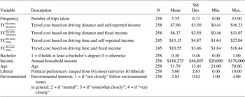
Furthermore, the mean household income for our sample was $118,275 (Table 1), which is substantially higher than the median household income of $62,704 for the County (US Census, 2023). This is potentially problematic because the higher the income level, the higher the opportunity time cost we assume in the travel cost variables. To mitigate this potential issue, we constructed the travel cost variables above with two different income measures. The first approach used the self-reported income measure for $ {Income}_i $
in Equation (4), and the second approach used a fixed value of $62,704 such that
$ {Income}_i $
in Equation (4), and the second approach used a fixed value of $62,704 such that $ {Income}_i=\overline{Income}=\$\mathrm{62,704} $
. Therefore, a total of four travel cost variables were used in our analysis:
$ {Income}_i=\overline{Income}=\$\mathrm{62,704} $
. Therefore, a total of four travel cost variables were used in our analysis: $ T{C}_{distance}^{Incom{e}_i} $
(based on driving distance and self-reported income),
$ T{C}_{distance}^{Incom{e}_i} $
(based on driving distance and self-reported income), $ T{C}_{distance}^{\overline{Income}} $
(based on driving distance and fixed income),
$ T{C}_{distance}^{\overline{Income}} $
(based on driving distance and fixed income), $ T{C}_{time}^{Incom{e}_i} $
(based on driving time and self-reported income) and
$ T{C}_{time}^{Incom{e}_i} $
(based on driving time and self-reported income) and $ T{C}_{time}^{\overline{Income}} $
(based on driving time and fixed income).
$ T{C}_{time}^{\overline{Income}} $
(based on driving time and fixed income).
Table 1. Descriptions and summary statistics of the variables

The quantity demanded, or trip frequency, was measured by asking the respondents to indicate how often they visited the drop-off center, from the following categories (five-trip increments): “I didn’t make any trips,” “1 to 5 trips,” “6 to 10 trips,” …, “36 to 40 trips” and “more than 40 trips.” For each category, the midpoint was assumed (e.g. 3 for “1 to 5 trips”). For the “I didn’t make any trips” category, 0 was assigned. Given that the dependent variable is the number of trips taken, count models were estimated. The first model included observations with zero trips and estimated the negative binomial model. The second model, on the other hand, excluded observations with zero trips by truncating at zero. Therefore, a total of eight regression models were estimated: negative binomial and truncated negative binomial for the four travel cost variables.
The survey also included other demographic questions, such as educational level, age, political preferences and overall interest in environmental issues. Therefore, $ \boldsymbol{\gamma}^{\prime }{\boldsymbol{X}}_{\boldsymbol{i}} $
in Equation (1) was specified as
$ \boldsymbol{\gamma}^{\prime }{\boldsymbol{X}}_{\boldsymbol{i}} $
in Equation (1) was specified as $ {\beta}_2{Bachelor}_i+{\beta}_3{Income}_i+{\beta}_4{Age}_i+{\beta}_5{Liberal}_i+{\beta}_6 Environmenta{l}_i $
. A total of 258 respondents responded to all survey questions used in our analysis.
$ {\beta}_2{Bachelor}_i+{\beta}_3{Income}_i+{\beta}_4{Age}_i+{\beta}_5{Liberal}_i+{\beta}_6 Environmenta{l}_i $
. A total of 258 respondents responded to all survey questions used in our analysis.
We further decided to remove observations that reported the “extreme values” for the trip frequency (1 respondent who chose “more than 40 trips”), driving distance (59 respondents who chose “more than 12 miles”) and driving time (3 respondents who chose “more than 30 minutes”) questions because (1) these categories do not have the upper bound, (2) arbitrary values must be assigned and (3) when arbitrary values were assigned, they either made the coefficient on travel cost statistically insignificant or inflated the CS estimates.Footnote 2 Table 1 presents descriptions and summary statistics of the variables used in our analysis.
Furthermore, we suspected that those who took their recyclables to the drop-off center might have run other errands. In other words, recycling might not have been the only purpose of the trips. Therefore, we included a survey question that asked if they ran other errands on their last trip to the drop-off center. Out of the 258 responses, 64 (25%) indicated that they dropped off recyclables and came home directly, 128 (50%) indicated that they dropped off recyclables and ran errands, 56 (22%) indicated that they did not remember and 10 (4%) indicated that they did not take any trips to the drop-off center in the past 6 months. These responses indicated that the driving cost would be overestimated if the round-trip distance were used in its calculation, because this assumes that the driving cost is exclusively for recycling. Therefore, we decided to use the one-way distance instead of the round-trip distance.Footnote 3
The per-trip CS per respondent can be calculated as $ -\frac{1}{{\hat{\beta}}_1} $
, where
$ -\frac{1}{{\hat{\beta}}_1} $
, where $ {\hat{\beta}}_1 $
is the estimated coefficient on the travel cost variable (Haab & McConnell, Reference Haab and McConnell2002). Given the CS measure is a nonlinear transformation of a coefficient, the delta method was used to construct the confidence interval. Following Greene (Reference Greene2012), the asymptotic variance of the CS was obtained as
$ {\hat{\beta}}_1 $
is the estimated coefficient on the travel cost variable (Haab & McConnell, Reference Haab and McConnell2002). Given the CS measure is a nonlinear transformation of a coefficient, the delta method was used to construct the confidence interval. Following Greene (Reference Greene2012), the asymptotic variance of the CS was obtained as
 $$ \hat{AVar}\left(\frac{1}{{\hat{\beta}}_1}\right)=\left[\frac{1}{{\hat{\beta}}_1^2}\right]\ast Var\left({\hat{\beta}}_1^2\right)\ast \left[\frac{1}{{\hat{\beta}}_1^2}\right]. $$
5. Results
Table 2 presents the negative binomial regression results, including observations with zero trips. The coefficient of $ \alpha $
is often referred to as the overdispersion coefficient, and the negative binomial model simplifies to Poisson when
$ \alpha $
is often referred to as the overdispersion coefficient, and the negative binomial model simplifies to Poisson when $ \alpha =0 $
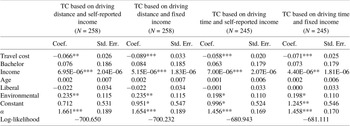
. In other words, when the estimated overdispersion coefficient is statistically different from zero, the negative binomial is more appropriate for the data than the Poisson.Footnote 4 The estimated overdispersion coefficient is statistically significant for all models.
$ \alpha =0 $
. In other words, when the estimated overdispersion coefficient is statistically different from zero, the negative binomial is more appropriate for the data than the Poisson.Footnote 4 The estimated overdispersion coefficient is statistically significant for all models.
Table 2. Negative binomial regression results, including observations with zero trips

Note: *, ** and *** denote 10, 5 and 1% confidence levels, respectively.
The coefficient on the travel cost variable is negative and statistically significant for both models, indicating that the number of trips taken (quantity demanded) decreases as the travel cost (price) of visiting the drop-off center increases. This finding is consistent with the law of demand. The coefficient on income is positive and statistically significant for all models, indicating that the quantity demanded increases as the income level increases. However, the magnitude of the coefficient is negligible. The coefficient on environmental interests is positive and statistically significant for the models with the travel cost variables based on driving distance, indicating that those who follow environmental issues more closely took more trips to the drop-off center. However, the coefficient is statistically significant only at the 10% level for the models with the travel cost variables based on driving time. Coefficients on the other socioeconomic factors included in the model are not statistically significant.
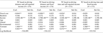
Table 3 presents the truncated negative binomial regression results, excluding observations with zero trips. Consistent with the results from the negative binomial models, the overdispersion coefficient is statistically significant for all models. The coefficient on travel cost, however, is statistically significant only for the models with the travel cost variables based on driving distance (i.e. $ T{C}_{distance}^{Incom{e}_i} $
and
$ T{C}_{distance}^{Incom{e}_i} $
and $ T{C}_{distance}^{\overline{Income}} $
). It is statistically significant only at the 10% level for the model with
$ T{C}_{distance}^{\overline{Income}} $
). It is statistically significant only at the 10% level for the model with $ T{C}_{time}^{Incom{e}_i} $
, and it is not statistically significant for the model with
$ T{C}_{time}^{Incom{e}_i} $
, and it is not statistically significant for the model with $ T{C}_{time}^{\overline{Income}} $
. The coefficient on income is still statistically significant, but the coefficient on environmental interests is not statistically significant. The statistically insignificant coefficients are potentially due to the smaller number of observations included in the model (i.e. Type-II error).
$ T{C}_{time}^{\overline{Income}} $
. The coefficient on income is still statistically significant, but the coefficient on environmental interests is not statistically significant. The statistically insignificant coefficients are potentially due to the smaller number of observations included in the model (i.e. Type-II error).
Table 3. Truncated negative binomial regression results, excluding observations with zero trips

Note: *, **, and *** denote 10, 5 and 1% confidence levels, respectively.
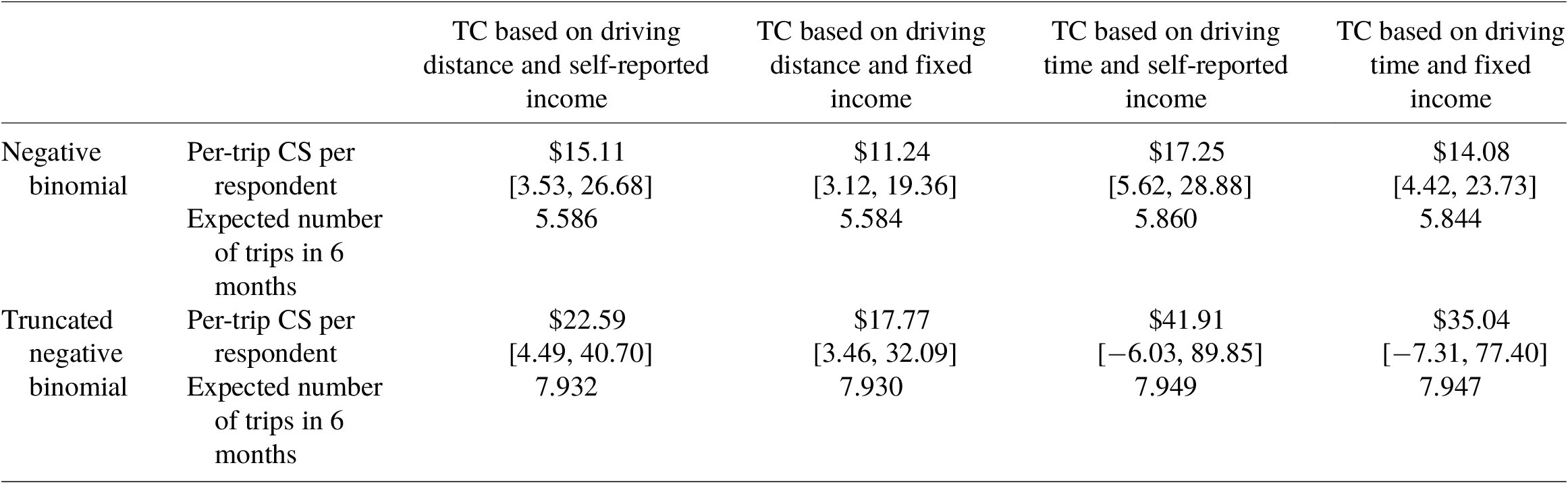
Table 4 presents the per-trip CS estimates from the regression results. The per-trip CS is the economic benefit a Monongalia County resident receives from taking recyclables to the drop-off center each time. From the negative binomial regression results, the per-trip CS is $15.11 per respondent when $ T{C}_{distance}^{Incom{e}_i} $
was used, $11.24 per respondent when
$ T{C}_{distance}^{Incom{e}_i} $
was used, $11.24 per respondent when $ T{C}_{distance}^{\overline{Income}} $
was used, $17.25 per respondent when
$ T{C}_{distance}^{\overline{Income}} $
was used, $17.25 per respondent when $ T{C}_{time}^{Incom{e}_i} $
was used and $14.08 per respondent when
$ T{C}_{time}^{Incom{e}_i} $
was used and $14.08 per respondent when $ T{C}_{time}^{\overline{Income}} $
was used. Overall, we find that the CS estimates are more conservative when driving distance is used to construct the travel cost variable, compared to using driving time. Also, using the fixed household income resulted in more conservative CS estimates, compared to using self-reported income. The 95% confidence intervals are reported in brackets, and the lower bound of the intervals is strictly positive for all cases, indicating that these CS estimates are statistically different from $0.
$ T{C}_{time}^{\overline{Income}} $
was used. Overall, we find that the CS estimates are more conservative when driving distance is used to construct the travel cost variable, compared to using driving time. Also, using the fixed household income resulted in more conservative CS estimates, compared to using self-reported income. The 95% confidence intervals are reported in brackets, and the lower bound of the intervals is strictly positive for all cases, indicating that these CS estimates are statistically different from $0.
Table 4. Consumer surplus estimates

Note: 95% confidence intervals are reported in the brackets.
From the truncated negative binomial regression results, we should expect higher CS values compared to those of the negative binomial regression results, given that observations with zero trips were excluded. The per-trip CS is $22.59 per respondent when $ T{C}_{distance}^{Incom{e}_i} $
was used, $17.77 per respondent when
$ T{C}_{distance}^{Incom{e}_i} $
was used, $17.77 per respondent when $ T{C}_{distance}^{\overline{Income}} $
was used, $41.91 per respondent when
$ T{C}_{distance}^{\overline{Income}} $
was used, $41.91 per respondent when $ T{C}_{time}^{Incom{e}_i} $
was used and $35.04 per respondent when
$ T{C}_{time}^{Incom{e}_i} $
was used and $35.04 per respondent when $ T{C}_{time}^{\overline{Income}} $
was used. However, the lower bound of the last two CS estimates is negative, indicating that the CS estimates are statistically not different from $0.
$ T{C}_{time}^{\overline{Income}} $
was used. However, the lower bound of the last two CS estimates is negative, indicating that the CS estimates are statistically not different from $0.
Table 4 also presents the expected number of trips in 6 months estimated from the regression models. By multiplying the per-trip CS per respondent by the expected number of trips, we can obtain the aggregate CS per respondent for 6 months. Using the estimates from the model with $ T{C}_{distance}^{\overline{Income}} $
(our most conservative estimates), the aggregate CS per respondent is $62.76 for 6 months from the negative binomial model and $140.92 for 6 months from the truncated negative binomial model. We can further obtain the annual CS per respondent by multiplying the aggregate CS per respondent by 2, assuming that the respondent’s behaviors would be consistent throughout the year. The annual CS per respondent is $125.52 from the negative binomial model and is $281.83 from the truncated negative binomial model. These are the economic benefits each County resident receives from participating in recycling throughout the year.
$ T{C}_{distance}^{\overline{Income}} $
(our most conservative estimates), the aggregate CS per respondent is $62.76 for 6 months from the negative binomial model and $140.92 for 6 months from the truncated negative binomial model. We can further obtain the annual CS per respondent by multiplying the aggregate CS per respondent by 2, assuming that the respondent’s behaviors would be consistent throughout the year. The annual CS per respondent is $125.52 from the negative binomial model and is $281.83 from the truncated negative binomial model. These are the economic benefits each County resident receives from participating in recycling throughout the year.
6. Discussion
Drop-off recycling is one of the most widely used recycling programs by local governments because it is less costly compared to curbside pickup (Saphores et al., Reference Saphores, Nixon, Ogunseitan and Shapiro2006; Sidique et al., Reference Sidique, Lupi and Joshi2013). It is also the most economical option in rural areas (Tiller et al., Reference Tiller, Jakus and Park1997). However, as Sidique et al. (Reference Sidique, Lupi and Joshi2013) argued, the demand for drop-off recycling programs has been overlooked in the literature. This study presents the first analysis in the literature that measured the economic benefit people receive from participating in drop-off recycling. Our findings indicated that the CS, the economic benefit a person receives from recycling, is $11.24–$17.25 each time they visit the drop-off center if the model includes observations with zero trips, and is $17.77–$41.91 if the model excludes observations with zero trips, depending on the travel cost specification. Using the most conservative estimates, our findings suggested that the annual CS per person is $125.52 when the model includes observations with zero trips and is $281.83 when the model excludes observations with zero trips.
The total CS would be the annual CS per respondent multiplied by the population of interest. Conceptually, the model that excludes observations with zero trips is expected to result in a higher per-person CS estimate, compared to the model that includes observations with zero trips. However, the population of interest between the two models is different. For the model that includes observations with zero trips, the population would be the total number of households in the County. For the model that excludes observations with zero trips, on the other hand, the population would be a subset of the County households that take their recyclables to the drop-off center. Therefore, the total CS estimates from the two models should be roughly the same, such that
 $$ Total\hskip0.32em C{S}_{nb}= Annual\hskip0.32em C{S}_{nb}\hskip0.32em \ast \hskip0.32em N\approx Total\hskip0.32em C{S}_{tnb}= Annual\hskip0.32em C{S}_{tnb}\hskip0.32em \ast \hskip0.32em n. $$
where the subscripts nb and tnb denote negative binomial and truncated negative binomial, respectively, N denotes the total number of households in the County and n denotes the number of county households that recycle at the drop-off center. There are roughly 10,500 households in Monongalia County to whom Republic Services provides its services. Therefore, N is known, and it is 10,500. However, information about the number of County residents who visit the drop-off center is not readily available. Solving Equation (8) for n,
 $$ n\approx \frac{Annual\hskip0.32em C{S}_{nb}}{Annual\hskip0.32em C{S}_{tnb}}\ast N=\frac{\$125.52\hskip0.32em }{\$281.83}\ast \mathrm{10,500}\approx \mathrm{4,676}. $$
Therefore, we estimate that of the 10,500 households to whom Republic Services provides services, 4,676 households recycle at the drop-off center and the total CS is $1,317,960 annually.
Another contribution of this study is the use of driving time in the construction of the travel cost variable. The use of driving time could be especially advantageous in analyzing the demand for recreational trips in high-traffic and congested areas, where the resource users’ decision to take trips might be heavily influenced by driving time rather than simple driving distance. As noted earlier, however, the coefficient on the travel cost variable where the driving time was used was statistically insignificant for the models that excluded observations with zero trips. These models likely suffer from type-II errors due to the smaller sample size resulting from dropping observations with zero trips. More research is needed to better understand the effectiveness of the use of driving time.
Lastly, TCM studies in the literature typically include a travel cost variable for a substitute site (Parsons, Reference Parsons, Champ, Boyle and Brown2003). Technically, there exist three recycling drop-off sites in Monongalia County (say sites 1, 2 and 3), but the drop-off center we focused on in this study (site 1) is the main center that the public uses. No information about the other sites is available on the Monongalia County recycling program website. In fact, we became aware of the other sites from a conversation with a representative from Republic Services when developing the survey instrument. In the survey, we included questions to gauge respondents’ awareness and visits to the other sites. Out of the 258 respondents, only 32 (12%) indicated that they were aware of site 2, and 6 of the 32 indicated that they took at least one trip. As for site 3, only 18 (7%) indicated that they were aware of the site, and 2 of the 18 indicated that they had taken at least one trip. Therefore, we concluded that there were no substitution behaviors and decided to focus on the main center. Monongalia County may need to provide more information about the other recycling drop-off sites to raise awareness and encourage recycling.

 Open access