


1. Introduction
On a stochastic basis $(\Omega, \mathcal{F}, {\mathbb{P}};\; \mathbb{F})$
, where
$(\Omega, \mathcal{F}, {\mathbb{P}};\; \mathbb{F})$
, where $\mathbb{F}=(\mathcal{F}_t)_{t\ge 0}$
is a (right-continuous) filtration, we consider a spectrally negative Lévy process
$\mathbb{F}=(\mathcal{F}_t)_{t\ge 0}$
is a (right-continuous) filtration, we consider a spectrally negative Lévy process $X=(X_t)_{t\ge 0}$
starting at
$X=(X_t)_{t\ge 0}$
starting at $x\in \mathbb{R}$
,
$x\in \mathbb{R}$
,
 \begin{align*}X_t = x + ct + \sigma W_t - L_t,\quad t\ge 0,\end{align*}
where $x,c\in \mathbb{R}$
are constants,
$x,c\in \mathbb{R}$
are constants, $W=(W_t)_{t\ge 0}$
is an
$W=(W_t)_{t\ge 0}$
is an $\mathbb{F}$
-Wiener process, and
$\mathbb{F}$
-Wiener process, and $L=(L_t)_{t\ge 0}$
is an
$L=(L_t)_{t\ge 0}$
is an $\mathbb{F}$
-Lévy subordinator (possibly of infinite activity) with the Lévy measure
$\mathbb{F}$
-Lévy subordinator (possibly of infinite activity) with the Lévy measure $\nu$
on
$\nu$
on $(0,\infty)$
satisfying
$(0,\infty)$
satisfying
 \begin{align*}\int_0^1 z\,\nu(\mathrm{d} z) < \infty,\quad \nu([1,\infty)) < \infty.\end{align*}
Note that $W_0=L_0=0$
a.s. The Laplace exponent of X is defined as
$W_0=L_0=0$
a.s. The Laplace exponent of X is defined as
 \begin{align*}\psi_X(\theta) \;:\!=\; \log \mathbb{E}[{\mathrm{e}}^{\theta (X_1 - x)}] = c\theta + \dfrac{\sigma^2}{2} \theta^2 +\int_0^\infty ({\mathrm{e}}^{-\theta z} -1)\,\nu(\mathrm{d} z),\quad \theta \ge 0.\end{align*}
We are interested in the q-scale function of X, $W^{(q)}\colon \mathbb{R}\to \mathbb{R}_+\;:\!=\; [0,\infty)$
for some
$W^{(q)}\colon \mathbb{R}\to \mathbb{R}_+\;:\!=\; [0,\infty)$
for some $q\ge 0$
, defined as follows:
$q\ge 0$
, defined as follows: $W^{(q)}(x) = 0$
on
$W^{(q)}(x) = 0$
on $(\!-\!\infty,0)$
and otherwise
$(\!-\!\infty,0)$
and otherwise $W^{(q)}$
is the unique continuous function that is right-continuous at the origin with the Laplace transform
$W^{(q)}$
is the unique continuous function that is right-continuous at the origin with the Laplace transform
 \begin{align*}\int_0^\infty {\mathrm{e}}^{-\theta z}W^{(q)}(z)\,\mathrm{d} z = \dfrac{1}{\psi_X(\theta) - q}\quad \text{for $\theta > \Phi(q)$},\end{align*}
where $\Phi(q)$
is called the Lundberg exponent:
$\Phi(q)$
is called the Lundberg exponent:
 \begin{align*}\Phi(q) \;:\!=\; \sup\{\theta \ge 0 \mid \psi_X(\theta) = q\}.\end{align*}
The scale functions play essential roles in fluctuation theory of Lévy processes and have various applications in insurance and finance. For example, defining two stopping times $\tau_\alpha^+=\inf\{t>0 \mid X_t>\alpha\}$
and
$\tau_\alpha^+=\inf\{t>0 \mid X_t>\alpha\}$
and $\tau_\alpha^- = \inf\{t>0 \mid X_t < \alpha\}$
for each
$\tau_\alpha^- = \inf\{t>0 \mid X_t < \alpha\}$
for each $\alpha\in \mathbb{R}$
, we have a fluctuation identity for
$\alpha\in \mathbb{R}$
, we have a fluctuation identity for $a>0$
such that
$a>0$
such that
 \begin{align*}\mathbb{E}\bigl[{\mathrm{e}}^{-q \tau_a^+}\boldsymbol{1}_{\{\tau_a^+ < \tau_0^-\}}\bigr] = \dfrac{W^{(q)}(x)}{W^{(q)}(a)} \quad \mbox{for $x \in [0,a]$},\end{align*}
which is an essential identity in the theory of two-sided exit problems and useful in analyzing credit risks and barrier options, among others. As $q=0$
, we have
$q=0$
, we have ${\mathbb{P}}(\tau_0^- <\tau_a^+) = 1 - W^{(0)}(x)/W^{(0)}(a)$
, and so assuming that
${\mathbb{P}}(\tau_0^- <\tau_a^+) = 1 - W^{(0)}(x)/W^{(0)}(a)$
, and so assuming that
 \begin{align*}\psi'(0+) = c - \int_0^\infty z\,\nu(\mathrm{d} z) >0,\end{align*}
called the net profit condition in ruin theory, which implies that $W^{(0)}(\infty) = 1/\psi'(0+)$
, we have the well-known identity for the ruin probability in classical ruin theory:
$W^{(0)}(\infty) = 1/\psi'(0+)$
, we have the well-known identity for the ruin probability in classical ruin theory:
 \begin{align}{\mathbb{P}}(\tau_0^- < \infty) = 1 - \psi'(0+)W^{(0)}(x). \end{align}
See Kyprianou [Reference Kyprianou14] for details regarding these identities. Moreover, Biffis and Kyprianou [Reference Biffis and Kyprianou5], as well as Feng and Shimizu [Reference Feng and Shimizu9], demonstrated that scale functions are useful tools for representing more general ruin-related risks. They showed that certain generalized Gerber–Shiu functions – whose classical version was introduced by Gerber and Shiu [Reference Gerber and Shiu10] – can also be expressed in terms of q-scale functions.
Scale functions also play a significant role in optimal dividend problems; see Loeffen [Reference Loeffen17]. Additionally, they are involved in the study of Parisian ruin probabilities, as explored by Loeffen et al. [Reference Loeffen, Czarna and Palmowski18] and Baurdoux et al. [Reference Baurdoux, Pardo, Perez and Renaud1], among others.
The connection between ruin theory and q-scale functions is deeply rooted in the potential theory of spectrally negative Lévy processes and the Wiener–Hopf factorization; see e.g. Bertoin [Reference Bertoin3, Reference Bertoin4] and Roger [Reference Roger20]. For further details, the reference lists in Kyprianou [Reference Kyprianou14], Kyprianou and Rivero [Reference Kyprianou and Rivero15], Feng and Shimizu [Reference Feng and Shimizu9], and Kuznetsov et al. [Reference Kuznetsov, Kyprianou and Rivero13] provide useful historical context and insights into their applications across various fields.
In considering such an application, it is important to recognize the practical need to identify the scale function and estimate it statistically from observations of a given Lévy process. Indeed, the identification and approximation of scale functions have attracted considerable attention in recent years.
We can find an explicit representation for some simple cases, such as compound Poisson processes; see e.g. Hubalek and Kyprianou [Reference Hubalek and Kyprianou11]. However, obtaining a general representation via the Laplace transform is generally challenging because Laplace inversion is too difficult to implement. Therefore, attempts have been made to obtain an approximate representation. The earliest work on an approximation of scale functions is due to Egami and Yamazaki [Reference Egami and Yamazaki8], who constructed an approximate sequence of q-scale functions using a compound Poisson-type Lévy process with phase-type jumps, forming a dense family in the class of spectrally negative Lévy processes. Landrault and Willmot [Reference Landrault and Willmot16] proposed an asymptotic expansion for Wiener–Poisson risk models by inverting the Laplace transform of scale functions and investigating some examples where explicit expansions are obtained. Behme et al. [Reference Behme, Oechsler and Schilling2] extended their results to more general Lévy processes with infinite jumps. Moreover, Xie et al. [Reference Xie, Cui and Zhang27] focused on a specific probabilistic representation of the q-scale function and provided an approximation formula using a Laguerre series expansion. See also Martín-González et al. [Reference Martín-González, Murillo-Salas and Pantí19] for an alternative expansion, and Surya [Reference Surya25] for numerical methods, among others.
Thus there are many discussions on the approximation of scale functions, but to the best of our knowledge, statistical inference based on underlying data has not yet been discussed. Our paper’s novelty lies not only in providing a new series approximation of the q-scale function but also a data-based statistical estimation of it. Among these, we are particularly concerned with problems in insurance actuarial practice. In modern actuarial practice, it is standard to use the spectrally negative Lévy process $X=(X_t)_{t\ge 0}$
for the surplus or asset processes of insurance companies, and certain discrete observations of X are available as real data; see Section 3.1. However, it is usually not clear from the data which Lévy process these data follow. We therefore propose a method for estimating scale functions without specifying a model of X, by using a non-parametric method for estimating quantities associated with the Lévy measure.
$X=(X_t)_{t\ge 0}$
for the surplus or asset processes of insurance companies, and certain discrete observations of X are available as real data; see Section 3.1. However, it is usually not clear from the data which Lévy process these data follow. We therefore propose a method for estimating scale functions without specifying a model of X, by using a non-parametric method for estimating quantities associated with the Lévy measure.
We must take two steps to identify the q-scale function in practice. First we introduce a new approximation formula. We focus on a compound geometric integral representation of the q-scale function obtained by Feng and Shimizu [Reference Feng and Shimizu9]. We derive a Laguerre series expansion of the corresponding compound geometric distribution function, and the Stieltjes integral with respect to it gives the expansion of the q-scale function. Although we also use a Laguerre expansion, as in Xie et al. [Reference Xie, Cui and Zhang27], our approach differs from theirs, and the formula is fundamentally different, which constitutes the primary contribution of this paper.
Second, we proceed to statistical inference. Two studies, by Zhang and Su [Reference Zhang and Su29] and Shimizu and Zhang [Reference Shimizu and Zhimin24], are instructive in this regard. The former proposes an estimator of Gerber–Shiu functions by deriving its Laguerre series expansion and estimating the coefficients for each term. They show the consistency of their proposed estimator. Shimizu and Zhang [Reference Shimizu and Zhimin24] applied the same approach to ruin probability and further showed that the estimator is asymptotically normal. As shown in equation (1.1), the ruin probability is represented by $W^{(0)}(x)$
, so their estimator is also an asymptotically normal estimator for the 0-scale function. This paper constructs an asymptotically normal estimator of the q-scale function, which generalizes the results of [Reference Shimizu and Zhimin24].
$W^{(0)}(x)$
, so their estimator is also an asymptotically normal estimator for the 0-scale function. This paper constructs an asymptotically normal estimator of the q-scale function, which generalizes the results of [Reference Shimizu and Zhimin24].
The paper is organized as follows. Section 2 introduces the series representation of the q-scale function obtained by Feng and Shimizu [Reference Feng and Shimizu9]. Under the net profit condition, the q-scale function has an integral representation in the form of the expected value of the compound geometric distribution. Section 3 covers statistical inference. Assuming X to be a surplus model, we construct auxiliary statistics for each unknown parameter under a reasonable discrete observation scheme. Finally, in Section 3.2, we construct an estimator for the Laguerre expansion of the q-scale function based on these auxiliary statistics. The proposed estimators are shown to be consistent and asymptotically normal. Supplementary lemmas are summarized in the Appendix.
Notation. Throughout the paper, we use the following notation.
-
• $\mathbb{N} = \{1,2,3,\ldots\}$
;
$\mathbb{N}_0\;:\!=\; \mathbb{N} \cup \{0\}$
;
$\mathbb{R}_+\;:\!=\; [0,\infty)$
.
$\mathbb{N} = \{1,2,3,\ldots\}$
;
$\mathbb{N}_0\;:\!=\; \mathbb{N} \cup \{0\}$
;
$\mathbb{R}_+\;:\!=\; [0,\infty)$
. -
• For a
$d\times d$
matrix
$A=(a_{ij})_{1\le i,j\le d}$
, let
$|A| \;:\!=\; \bigl( \sum_{i,j=1}^d a_{ij}^2 \bigr)^{1/2}$
. -
• For
$\boldsymbol{a}=(a_1,\ldots,a_d)^\top$
and
${\boldsymbol{b}}=(b_1,\ldots,b_d)^\top$
, the inner product is defined by
$\boldsymbol{a}\cdot {\boldsymbol{b}} =\sum_{k=1}^d a_kb_k$
. -
• Let
${\boldsymbol 0}_d$
denote the zero vector of dimension d, and let
$I_d$
be the
$d\times d$
identity matrix. Moreover,
$N_d(\boldsymbol{a}, \Sigma)$
denotes the d-dim Gaussian distribution with mean vector
$\boldsymbol{a}$
and covariance matrix
$\Sigma$
. In particular,
$N\;:\!=\; N_1$
. -
• The indicator function on a set
$A\subset \mathbb{R}$
is given by
$\boldsymbol{1}_A(x) = 1$
if
$x\in A$
; 0 otherwise. -
• For functions f, g on
$\mathbb{R}$
, let
$f(x) \lesssim g(x)$
if there exists a constant
$C>0$
such that
$f(x) \le C g(x)$
for any
$x\in \mathbb{R}$
. -
• For a function
$f(x_1,x_2,\ldots,x_d)$
, let
\begin{align*} \partial_{x_i} f \;:\!=\; \frac{\partial f}{\partial x_i}\quad\text{and}\quad \partial_{(x_1,\ldots,x_d)} f = (\partial_{x_1} f,\ldots, \partial_{x_d}f)^\top. \end{align*}
-
• For
$s\ge 1$
and
$\alpha>0$
, let In particular, we let
\begin{align*}L^s_\alpha(\mathbb{R}_+) = \biggl\{f\colon \mathbb{R}_+\to \mathbb{R}\,\colon \, \int_0^\infty f^s(x)\,{\mathrm{e}}^{-\alpha x}\,\mathrm{d} x < \infty \biggr\}.\end{align*}
$L^s(\mathbb{R}_+) \;:\!=\; L^s_0(\mathbb{R}_+)$
, and for
$f,g\in L^2(\mathbb{R}_+)$
,
\begin{align*}\langle f,g\rangle \;:\!=\; \int_0^\infty f(x)g(x)\,\mathrm{d} x,\quad \|f\|\;:\!=\; \sqrt{\langle f,f\rangle}.\end{align*}
-
• For functions f, g on
$\mathbb{R}_+$
of finite variation, the convolution is defined as Moreover, the kth convolution is defined by
\begin{align*}f*g (x) \;:\!=\; \int_{[0,x]}f(x-y)g(y)\,\mathrm{d} y,\quad x\ge 0.\end{align*}
$f^{*0}= \delta_0$
(Dirac’s delta function concentrated on 0) and
$f^{*k} = f*f^{*(k-1)}$
for
$k\in \mathbb{N}$
.
-
• For a measure
$\nu$
on
$\mathbb{R}_+$
and a function
${\boldsymbol{f}}=(f_1,\ldots,f_d)^\top\colon \mathbb{R}_+\to \mathbb{R}^d$
, we let
\begin{align*}\nu({\boldsymbol{f}}) \;:\!=\; \int_{\mathbb{R}_+} {\boldsymbol{f}}(x)\,\nu(\mathrm{d} x) = \biggl(\int_{\mathbb{R}_+} f_1(x)\,\nu(\mathrm{d} x),\ldots,\int_{\mathbb{R}_+} f_d(x)\,\nu(\mathrm{d} x)\biggr)^\top.\end{align*}


2. Series representation of q-scale functions
2.1. A compound geometric representation of q-scale functions
A closed-form expression for the q-scale function of the process X was derived by Feng and Shimizu [Reference Feng and Shimizu9] as an expectation with respect to a compound geometric distribution under the following net profit condition:
NPC $\displaystyle c > \int_0^\infty z\,\nu(\mathrm{d} z)$
.
$\displaystyle c > \int_0^\infty z\,\nu(\mathrm{d} z)$
.
To state the representation of $W^{(q)}$
, we prepare some notation. We will fix a number
$W^{(q)}$
, we prepare some notation. We will fix a number $q\ge 0$
for
$q\ge 0$
for $W^{(q)}$
, and let
$W^{(q)}$
, and let
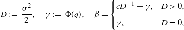 \begin{align*}D\;:\!=\; \dfrac{\sigma^2}{2},\quad \gamma\;:\!=\; \Phi(q),\quad\beta=\begin{cases}cD^{-1} + \gamma, & D>0, \\[5pt] \gamma, & D=0,\end{cases}\end{align*}
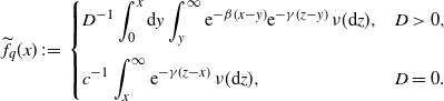 \begin{align*}\widetilde{f}_q(x) \;:\!=\;\begin{cases} \displaystyle D^{-1}\int_0^x \mathrm{d} y \int_y^{\infty} {\mathrm{e}}^{-\beta(x-y)}{\mathrm{e}}^{-\gamma(z-y)}\,\nu(\mathrm{d} z), & D > 0, \\[13pt] \displaystyle c^{-1}\int_x^{\infty} {\mathrm{e}}^{-\gamma(z-x)}\,\nu(\mathrm{d} z), & D=0.\end{cases} \end{align*}
We define a distribution $F_q$
with a probability density obtained from the function
$F_q$
with a probability density obtained from the function $\widetilde{f}_q$
:
$\widetilde{f}_q$
:
 \begin{align*}F_q(x) \;:\!=\; \int_0^x f_q(z)\,\mathrm{d} z,\quad f_q(z) = p^{-1} \widetilde{f}_q(z),\quad p \;:\!=\; \int_0^\infty \widetilde{f}_q(z)\,\mathrm{d} z.\end{align*}
In fact, $p\in (0,1)$
under the NPC condition and the probability density
$p\in (0,1)$
under the NPC condition and the probability density $f_q$
is well-defined; see Lemma C.1. Then the following representation is the immediate consequence from Feng and Shimizu [Reference Feng and Shimizu9, Proposition 4.1].
$f_q$
is well-defined; see Lemma C.1. Then the following representation is the immediate consequence from Feng and Shimizu [Reference Feng and Shimizu9, Proposition 4.1].
Lemma 2.1. Suppose the NPC condition for the process X. Then the q-scale function $W^{(q)}$
of X has the following integral form:
$W^{(q)}$
of X has the following integral form:
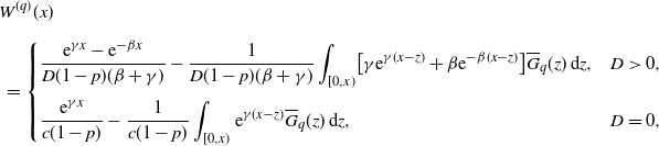 \begin{align*}& W^{(q)}(x) \\[5pt] &\ = \begin{cases} \displaystyle \dfrac{{\mathrm{e}}^{\gamma x} - {\mathrm{e}}^{-\beta x}}{D(1-p)(\beta+ \gamma)} - \dfrac{1}{D(1-p)(\beta+ \gamma)}\int_{[0,x)} \bigl[\gamma {\mathrm{e}}^{\gamma(x-z)} + \beta {\mathrm{e}}^{-\beta(x-z)}\bigr] \overline{G}_q(z)\,\mathrm{d} z, & D>0, \\[13pt] \displaystyle \dfrac{{\mathrm{e}}^{\gamma x}}{c(1-p)} - \dfrac{1}{c(1-p)}\int_{[0,x)} {\mathrm{e}}^{\gamma(x-z)}\overline{G}_q(z)\,\mathrm{d} z, & D=0,\end{cases} \end{align*}
where $p\in (0,1)$
and
$p\in (0,1)$
and $G_q$
is a compound geometric distribution function
$G_q$
is a compound geometric distribution function
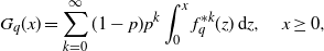 \begin{align}G_q(x) = \sum_{k=0}^\infty (1-p)p^k \int_0^x f_q^{*k}(z)\,\mathrm{d} z,\quad x\ge 0, \end{align}
and $G_q(x)\equiv 0$
for
$G_q(x)\equiv 0$
for $x<0$
.
$x<0$
.
Proof. See Section C.4.
2.2. Laguerre series expansion
Let $L_k(x)$
be the Laguerre polynomial of order k,
$L_k(x)$
be the Laguerre polynomial of order k,
 \begin{align*}L_k(x) = \dfrac{1}{n!}{\mathrm{e}}^x \dfrac{\mathrm{d}^n}{\mathrm{d} x^n} ({\mathrm{e}}^{-x}x^n) = \sum_{j=0}^k \binom{k}{j} \dfrac{(\!-\!x)^j}{j!}, \quad x\in \mathbb{R}_+\;:\!=\; [0,\infty),\end{align*}
by which we define the Laguerre function for each $\alpha>0$
as follows:
$\alpha>0$
as follows:
 \begin{align*}\varphi_{\alpha,k}(x) \;:\!=\; \sqrt{2\alpha}L_k(2\alpha x) \,{\mathrm{e}}^{-\alpha x},\quad x\in \mathbb{R}_+.\end{align*}
Note that the system $\{\varphi_{\alpha,k}\}_{k\in \mathbb{N}_0}$
consists of an orthogonal basis of
$\{\varphi_{\alpha,k}\}_{k\in \mathbb{N}_0}$
consists of an orthogonal basis of $L^2(\mathbb{R}_+)$
satisfying
$L^2(\mathbb{R}_+)$
satisfying
 \begin{align}\sup_{k\in \mathbb{N}_0,x\in \mathbb{R}_+}|\varphi_{\alpha,k}(x)|\le \sqrt{2\alpha }, \end{align}
and that for any $k\in \mathbb{N}_0$
, there exists some
$k\in \mathbb{N}_0$
, there exists some $\delta>0$
such that
$\delta>0$
such that
 \begin{align*}\varphi_{\alpha,k}(x) = {\mathrm{O}} \big({\mathrm{e}}^{-(\alpha - \delta)x}\big),\quad x\to \infty,\end{align*}
since $L_k$
is a polynomial of order k. Therefore we can control the decay order of the function
$L_k$
is a polynomial of order k. Therefore we can control the decay order of the function $\varphi_{k,\alpha}$
by choosing
$\varphi_{k,\alpha}$
by choosing $\alpha>0$
; see Remark 2.1.
$\alpha>0$
; see Remark 2.1.
Let $\mathcal{W}_\alpha^r(\mathbb{R}_+)$
be the Sobolev–Laguerre space (Bongioanni and Torrea [Reference Bongioanni and Torrea6]) for
$\mathcal{W}_\alpha^r(\mathbb{R}_+)$
be the Sobolev–Laguerre space (Bongioanni and Torrea [Reference Bongioanni and Torrea6]) for $\alpha, r>0$
:
$\alpha, r>0$
:
 \begin{align*}\mathcal{W}_\alpha^r(\mathbb{R}_+) \;:\!=\; \Biggl\{ f\in L^2(\mathbb{R}_+) \colon \sum_{k=0}^\infty k^r |\langle f,\varphi_{\alpha,k}\rangle|^2 < \infty\Biggr\}.\end{align*}
There are many useful connections between Laguerre systems and the Sobolev–Laguerre space, as discussed in Comte and Genon-Catalot [Reference Comte and Genon-Catalot7]. In particular, Proposition 7.1 and its remark provide an equivalent condition for a function to belong to $\mathcal{W}_\alpha^r(\mathbb{R}_+)$
, as follows.
$\mathcal{W}_\alpha^r(\mathbb{R}_+)$
, as follows.
Lemma 2.2. (Comte and Genon-Catalot [Reference Comte and Genon-Catalot7].) Let $r\in \mathbb{N}$
and
$r\in \mathbb{N}$
and $\alpha>0$
. Then
$\alpha>0$
. Then $f\in \mathcal{W}_\alpha^r(\mathbb{R}_+)$
if and only if f admits the derivatives of order r and that
$f\in \mathcal{W}_\alpha^r(\mathbb{R}_+)$
if and only if f admits the derivatives of order r and that
 \begin{align}x^{m/2} \partial_x^m f(x) \in L^2_\alpha(\mathbb{R}_+),\quad 0\le m\le r. \end{align}
The following uniform convergence of the Laguerre series expansion is obtained by Shimizu and Zhang [Reference Shimizu and Zhimin24, Proposition 3].
Lemma 2.3. For any $K\in \mathbb{N}$
, the partial sum of the Laguerre series expansion of
$K\in \mathbb{N}$
, the partial sum of the Laguerre series expansion of $f\in \mathcal{W}_\alpha^r(\mathbb{R}_+)$
,
$f\in \mathcal{W}_\alpha^r(\mathbb{R}_+)$
,
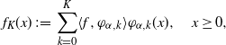 \begin{align*}f_K(x)\;:\!=\; \sum_{k=0}^K \langle f,\varphi_{\alpha,k}\rangle \varphi_{\alpha,k}(x),\quad x\ge 0,\end{align*}
satisfies
 \begin{align*}\sup_{x\in \mathbb{R}_+} |f_K(x) - f(x)| = {\mathrm{O}}(K^{-(r-1)/2}),\quad K\to \infty.\end{align*}
2.3. Laguerre expansion of
$\overline{\boldsymbol{G}}_{\boldsymbol{q}}$

According to Willmot and Lin [Reference Willmot and Lin26], for example, we see that the tail function $\overline{G}_q\;:\!=\; 1 - G_q$
should satisfy the following defective renewal equation (DRE):
$\overline{G}_q\;:\!=\; 1 - G_q$
should satisfy the following defective renewal equation (DRE):
 \begin{align} \overline{G}_q(x) = p\overline{F}_q + pf_q(x)* \overline{G}_q(x),\quad x\ge 0. \end{align}
We have the Laguerre expansion of $pf_q$
,
$pf_q$
, $p\overline{F}_q$
, and
$p\overline{F}_q$
, and $\overline{G}_q$
since these belong to
$\overline{G}_q$
since these belong to $L^2(\mathbb{R}_+)$
as shown in Section C.1: for
$L^2(\mathbb{R}_+)$
as shown in Section C.1: for $x\ge 0$
,
$x\ge 0$
,
 \begin{align*}pf_{q}(x)=\sum_{k=0}^{\infty}a^{f}_{\alpha,k}\varphi_{\alpha,k}(x),\quad p\overline{F}_{q}(x)=\sum_{k=0}^{\infty}a^{F}_{\alpha,k}\varphi_{\alpha,k}(x),\quad\overline{G}_{q}(x)=\sum_{k=0}^{\infty}a^{G}_{\alpha,k}\varphi_{\alpha,k}(x), \end{align*}
where $a^{f}_{\alpha,k}\;:\!=\; \langle pf_{q}, \varphi_{\alpha,k}\rangle$
,
$a^{f}_{\alpha,k}\;:\!=\; \langle pf_{q}, \varphi_{\alpha,k}\rangle$
, $a^{F}_{\alpha,k}\;:\!=\; \langle p\overline{F}_{q}, \varphi_{\alpha,k}\rangle$
, and
$a^{F}_{\alpha,k}\;:\!=\; \langle p\overline{F}_{q}, \varphi_{\alpha,k}\rangle$
, and $a^{G}_{\alpha,k}\;:\!=\; \langle \overline{G}_{q}, \varphi_{\alpha,k}\rangle$
.
$a^{G}_{\alpha,k}\;:\!=\; \langle \overline{G}_{q}, \varphi_{\alpha,k}\rangle$
.
For arbitrary $K\in \mathbb{N}_0$
, letting
$K\in \mathbb{N}_0$
, letting
 \begin{align*}\boldsymbol{a}^{f}_{\alpha,K}&\;:\!=\; \bigl(a^{f}_{\alpha,0},a^{f}_{\alpha,1},\ldots,a^{f}_{\alpha,K}\bigr)^{\top}, \\[5pt] \boldsymbol{a}^{F}_{\alpha,K}&\;:\!=\; \bigl(a^{F}_{\alpha,0},a^{F}_{\alpha,1},\ldots,a^{F}_{\alpha,K}\bigr)^{\top}, \\[5pt] \boldsymbol{a}^{G}_{\alpha,K}&\;:\!=\; \bigl(a^{G}_{\alpha,0},a^{G}_{\alpha,1},\ldots,a^{G}_{\alpha,K}\bigr)^{\top},\end{align*}
we have the following relation among these coefficients; see Zhang and Su [Reference Zhang and Su28, Section 2] or Shimizu and Zhang [Reference Shimizu and Zhimin24, Proposition 2].
Lemma 2.4. Define a $(K+1)\times(K+1)$
-matrix
$(K+1)\times(K+1)$
-matrix $A^f_{K}=(a_{kl})_{1\le k,l\le K+1}$
, whose components are given as follows:
$A^f_{K}=(a_{kl})_{1\le k,l\le K+1}$
, whose components are given as follows:
 \begin{align*} a_{kl}\;:\!=\; \begin{cases} 1-\dfrac{1}{\sqrt{2\alpha}}a^{f}_{\alpha,0}, &k=l,\\[13pt] -\dfrac{1}{\sqrt{2\alpha}}\bigl(a^{f}_{\alpha,k-l}-a^{f}_{\alpha,k-l-1}\bigr),&k>l,\\[7pt] 0,&k<l. \end{cases}\end{align*}
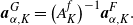
Then the matrix $A^f_K$
is invertible, and it holds that
$A^f_K$
is invertible, and it holds that
 \begin{align*}\boldsymbol{a}^{G}_{\alpha,K}= \bigl(A^f_{K}\bigr)^{-1} \boldsymbol{a}^{F}_{\alpha,K}.\end{align*}
Using this system, we can construct a Laguerre expansion of $\overline{G}_q(x)$
: for a vector
$\overline{G}_q(x)$
: for a vector ${\boldsymbol \varphi}_{\alpha,K} = (\varphi_{\alpha,0},\varphi_{\alpha,1},\ldots,\varphi_{\alpha,K})^\top$
,
${\boldsymbol \varphi}_{\alpha,K} = (\varphi_{\alpha,0},\varphi_{\alpha,1},\ldots,\varphi_{\alpha,K})^\top$
,
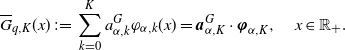 \begin{align}\overline{G}_{q,K}(x)\;:\!=\; \sum_{k=0}^K a_{\alpha,k}^G \varphi_{\alpha,k}(x) = \boldsymbol{a}^{G}_{\alpha,K}\cdot {\boldsymbol \varphi}_{\alpha,K} ,\quad x\in \mathbb{R}_+. \end{align}
Lemma 2.5. Suppose the tail function of the Lévy measure $\nu$
, say
$\nu$
, say $\overline{\nu}(x)\;:\!=\; \int_x^\infty \nu(\mathrm{d} z)$
, admits derivatives up to order
$\overline{\nu}(x)\;:\!=\; \int_x^\infty \nu(\mathrm{d} z)$
, admits derivatives up to order $r > 1$
and that the distribution
$r > 1$
and that the distribution $G_q$
given in (2.1) has moments of any polynomial order. Moreover, suppose there exists a constant
$G_q$
given in (2.1) has moments of any polynomial order. Moreover, suppose there exists a constant $\kappa>0$
such that
$\kappa>0$
such that
 \begin{align}\partial_x^m \overline{\nu}(x) = {\mathrm{O}} (1 + x^\kappa), \quad x\to \infty, \end{align}
for any $0\le m \le r-2$
. Then we have
$0\le m \le r-2$
. Then we have $\overline{G}_q \in \mathcal{W}_\alpha^r(\mathbb{R}_+)$
, and therefore
$\overline{G}_q \in \mathcal{W}_\alpha^r(\mathbb{R}_+)$
, and therefore
 \begin{align}\sup_{x\in \mathbb{R}_+}\bigl|\overline{G}_{q,K}(x) - \overline{G}_q(x)\bigr| = {\mathrm{O}} (K^{-(r-1)/2}) \to 0,\quad K\to \infty. \end{align}
Furthermore, if the condition (2.6) is much milder, such as
 \begin{align}\partial_x^m \overline{\nu}(x) = {\mathrm{O}}( {\mathrm{e}}^{\kappa x}), \quad x\to \infty, \end{align}
then the consequence (2.7) also holds if we choose $\alpha > 2\kappa$
.
$\alpha > 2\kappa$
.
Proof. See Section C.5.
Remark 2.1. Lemma 2.5 explains the significance of the tuning parameter $\alpha>0$
in the Laguerre function. When considering a model in which the Lévy measure satisfies (2.8), we can choose
$\alpha>0$
in the Laguerre function. When considering a model in which the Lévy measure satisfies (2.8), we can choose $\alpha$
such that
$\alpha$
such that $a>2\kappa$
. However, in most standard cases where (2.6) holds, we can choose any
$a>2\kappa$
. However, in most standard cases where (2.6) holds, we can choose any $\alpha>0$
; in particular, setting
$\alpha>0$
; in particular, setting $\alpha =1$
is both simple and sufficient.
$\alpha =1$
is both simple and sufficient.
2.4. Laguerre-type expansion for q-scale functions
We can obtain a series expansion of the q-scale function by replacing $\overline{G}_q(z)$
in the expression of
$\overline{G}_q(z)$
in the expression of $W^{(q)}$
in Lemma 2.1 with the corresponding Laguerre expansion (2.5).
$W^{(q)}$
in Lemma 2.1 with the corresponding Laguerre expansion (2.5).
Definition 2.1. For any $K\in \mathbb{N}$
and
$K\in \mathbb{N}$
and $\alpha>0$
, the Kth-Laguerre-type expansion of
$\alpha>0$
, the Kth-Laguerre-type expansion of $W^{(q)}$
, say
$W^{(q)}$
, say $W^{(q)}_K$
, is given by
$W^{(q)}_K$
, is given by
 \begin{align}W^{(q)}_K(x) \;:\!=\; P(x;\;p,\gamma,D) - {\boldsymbol{Q}}_{\alpha,K}(x;\;p,\gamma,D)\cdot \boldsymbol{a}^G_{\alpha,K}, \end{align}
where ${\boldsymbol{Q}}_{\alpha,K}\;:\!=\; (Q_{\alpha,0}, Q_{\alpha,1},\ldots, Q_{\alpha,K})^\top$
with
${\boldsymbol{Q}}_{\alpha,K}\;:\!=\; (Q_{\alpha,0}, Q_{\alpha,1},\ldots, Q_{\alpha,K})^\top$
with
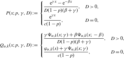 \begin{align*}P(x;\;p,\gamma,D)&\;:\!=\;\begin{cases} \dfrac{{\mathrm{e}}^{\gamma x}-{\mathrm{e}}^{-\beta x}}{D(1-p)(\beta+\gamma)},&D>0,\\[9pt] \dfrac{{\mathrm{e}}^{\gamma x}}{c(1-p)},&D=0,\end{cases} \\[9pt] Q_{\alpha,k}(x;\;p,\gamma,D)&\;:\!=\;\begin{cases} \dfrac{\gamma \Psi_{\alpha,k}(x;\;\gamma)+\beta\Psi_{\alpha,k}(x;\;-\beta)}{D(1-p)(\beta+\gamma)},&D>0,\\[9pt] \dfrac{\varphi_{\alpha,k}(x)+\gamma \Psi_{\alpha,k}(x;\;\gamma)}{c(1-p)},&D=0, \end{cases}\end{align*}
and
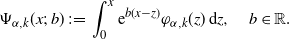 \begin{align}\Psi_{\alpha,k}(x;\;b)\;:\!=\; \int_{0}^x {\mathrm{e}}^{b(x-z)}\varphi_{\alpha,k}(z)\,\mathrm{d} z,\quad b \in \mathbb{R}. \end{align}
Remark 2.2. There is an alternative version of the q-scale function $Z^{(q)}\colon \mathbb{R} \to [1,\infty)$
, defined as
$Z^{(q)}\colon \mathbb{R} \to [1,\infty)$
, defined as
 \begin{align*}Z^{(q)}(x) = 1 + q\int_0^x W^{(q)}(z)\,\mathrm{d} z, \quad x\in \mathbb{R},\end{align*}
where we regard that $\int_0^x = 0$
if
$\int_0^x = 0$
if $x<0$
. Note that
$x<0$
. Note that $W^{(q)}(x) = q^{-1} \partial_x Z^{(q)}(x)$
as
$W^{(q)}(x) = q^{-1} \partial_x Z^{(q)}(x)$
as $q\ne 0$
. The Laguerre-type expansion of
$q\ne 0$
. The Laguerre-type expansion of $Z^{(q)}$
is also defined as
$Z^{(q)}$
is also defined as
 \begin{align}Z^{(q)}_K(x) &= 1 + q \int_0^x W^{(q)}_K(z)\,\mathrm{d} z \notag\\[5pt] &= 1 + q\bigl[ P^*(x;\; p,\gamma,D) - {\boldsymbol{Q}}^*_{\alpha,K}(x;\;p,\gamma,D)\cdot \boldsymbol{a}^G_{\alpha,K}\bigr], \end{align}
where ${\boldsymbol{Q}}^*_{\alpha,K}\;:\!=\; \bigl(Q^*_{\alpha,0}, Q^*_{\alpha,1},\ldots, Q^*_{\alpha,K}\bigr)^\top$
with
${\boldsymbol{Q}}^*_{\alpha,K}\;:\!=\; \bigl(Q^*_{\alpha,0}, Q^*_{\alpha,1},\ldots, Q^*_{\alpha,K}\bigr)^\top$
with
 \begin{align*}P^*(z;\;p,\gamma,D)&\;:\!=\; \left\{ \begin{aligned} &\dfrac{\gamma^{-1}(1 - {\mathrm{e}}^{\gamma x})-\beta^{-1}(1-{\mathrm{e}}^{-\beta x})}{D(1-p)(\beta+\gamma)},&D>0,\\[5pt] &\dfrac{1 - {\mathrm{e}}^{\gamma x}}{\gamma c(1-p)},&D=0, \end{aligned}\right. \\[5pt] Q^*_{\alpha,k}(x;\;p,\gamma,D)&\;:\!=\; \left\{ \begin{aligned} &\dfrac{\Psi_{\alpha,k}(x;\;\gamma) - \Psi_{\alpha,k}(x;\;-\beta)}{D(1-p)(\beta+\gamma)},&D>0,\\[5pt] &\dfrac{\Psi_{\alpha,k}(x;\;\gamma)}{c(1-p)},&D=0. \end{aligned}\right.\end{align*}
According to Lemma 2.3, if $\overline{G}_q \in \mathcal{W}_\alpha^r(\mathbb{R}_+)$
(e.g.
$\overline{G}_q \in \mathcal{W}_\alpha^r(\mathbb{R}_+)$
(e.g. $f\;:\!=\; \overline{G}_q$
satisfies (2.3)), then
$f\;:\!=\; \overline{G}_q$
satisfies (2.3)), then
 \begin{align*}\sup_{x\in \mathbb{R}_+}|W^{(q)}_K(x) - W^{(q)}(x)| \to 0,\quad K\to \infty;\end{align*}
see (2.7). Therefore it follows for any compact sets $V\subset \mathbb{R}_+$
that
$V\subset \mathbb{R}_+$
that
 \begin{align*}\sup_{x\in V}|Z^{(q)}_K(x) - Z^{(q)}(x)| \to 0,\quad K\to \infty.\end{align*}
Remark 2.3. The approximation formulas obtained in equations (2.9) and (2.11) are fundamentally different from those in Xie et al. [Reference Xie, Cui and Zhang27], while being more elementary. Their approximation focuses on the relationship between the probability density of the ‘killed process’ $X_{e_t}$
(where
$X_{e_t}$
(where $e_t$
is an exponential random variable with mean 1) and its scale function, cleverly expanding the probability density into a Laguerre series. In our approximation, we utilize a Laguerre series expansion for the compound geometric distribution
$e_t$
is an exponential random variable with mean 1) and its scale function, cleverly expanding the probability density into a Laguerre series. In our approximation, we utilize a Laguerre series expansion for the compound geometric distribution $\overline{G}_q$
, which is essentially similar to the approach of Shimizu and Zhang [Reference Shimizu and Zhimin24]. The utility of this approach becomes apparent in the subsequent discussion.
$\overline{G}_q$
, which is essentially similar to the approach of Shimizu and Zhang [Reference Shimizu and Zhimin24]. The utility of this approach becomes apparent in the subsequent discussion.
3. Statistical inference: main theorems
We will proceed with the statistical estimation of scale functions. When considering the practical application of q-scale functions, we typically focus on actuarial science, where $X=(X_t)_{t\ge 0}$
represents the dynamics of an insurance surplus model. In this context, the coefficient of the linear term, c, corresponds to the premium rate. Therefore, in this paper, we specifically treat the value of c as known.
$X=(X_t)_{t\ge 0}$
represents the dynamics of an insurance surplus model. In this context, the coefficient of the linear term, c, corresponds to the premium rate. Therefore, in this paper, we specifically treat the value of c as known.
3.1. Sampling scheme
Let $n\in \mathbb{N}$
. We assume that the process
$n\in \mathbb{N}$
. We assume that the process $X=(X_t)_{t\ge 0}$
is observed at discrete time points
$X=(X_t)_{t\ge 0}$
is observed at discrete time points $t_i^n\;:\!=\; i\Delta_n\ (i=0,1,\ldots,n)$
for some number
$t_i^n\;:\!=\; i\Delta_n\ (i=0,1,\ldots,n)$
for some number $\Delta_n>0$
:
$\Delta_n>0$
:
 \begin{align*}{\boldsymbol{X}}^n\;:\!=\; \{X_{t_i^n} \mid i = 0,1,\ldots, n\}, \quad T_n\;:\!=\; n\Delta_n.\end{align*}
In particular, the initial value $X_{t_0^n} = x$
is assumed to be known. Moreover, we assume that ‘large’ jumps of X are observed. That is, for some number
$X_{t_0^n} = x$
is assumed to be known. Moreover, we assume that ‘large’ jumps of X are observed. That is, for some number ${\epsilon}_n>0$
, we can identify the jumps whose sizes are larger than
${\epsilon}_n>0$
, we can identify the jumps whose sizes are larger than ${\epsilon}_n$
, which are finitely many on
${\epsilon}_n$
, which are finitely many on $[0,T_n]$
:
$[0,T_n]$
:
 \begin{align*}{\boldsymbol{J}}^n\;:\!=\; \{\Delta X_t\;:\!=\; X_t - X_{t-} \mid t\in [0,T_n],\ |\Delta X_t| > {\epsilon}_n \}.\end{align*}
Assume that we have data ${\boldsymbol{X}}^n \cup {\boldsymbol{J}}^n$
, and consider the following asymptotics:
${\boldsymbol{X}}^n \cup {\boldsymbol{J}}^n$
, and consider the following asymptotics:
 \begin{align}\Delta_n\to 0,\quad T_n\to \infty,\quad {\epsilon}_n\to 0, \end{align}
as $n\to \infty$
. We shall always use the limit
$n\to \infty$
. We shall always use the limit $n\to \infty$
when considering the asymptotic symbols, and assume (3.1) for the sampling scheme
$n\to \infty$
when considering the asymptotic symbols, and assume (3.1) for the sampling scheme $(\Delta_n,T_n,{\epsilon}_n)$
without further comment.
$(\Delta_n,T_n,{\epsilon}_n)$
without further comment.
Remark 3.1. The data ${\boldsymbol{X}}^n$
are assumed to represent the data on the remaining reserves that insurance companies record on a regular basis. On the other hand,
${\boldsymbol{X}}^n$
are assumed to represent the data on the remaining reserves that insurance companies record on a regular basis. On the other hand, ${\boldsymbol{J}}^n$
are assumed to be ‘large’ claims. It may seem unnatural to consider such a model with infinitely many jumps when modeling insurance surplus, but this is a standard surplus approximation in risk theory. Arguing under asymptotics such as (3.1) with data like
${\boldsymbol{J}}^n$
are assumed to be ‘large’ claims. It may seem unnatural to consider such a model with infinitely many jumps when modeling insurance surplus, but this is a standard surplus approximation in risk theory. Arguing under asymptotics such as (3.1) with data like ${\boldsymbol{J}}^n$
is a common way of theoretically justifying that the more detailed claims data you collect, the better the estimation. In practice, it is not necessary to observe infinitely many ‘small’ jumps.
${\boldsymbol{J}}^n$
is a common way of theoretically justifying that the more detailed claims data you collect, the better the estimation. In practice, it is not necessary to observe infinitely many ‘small’ jumps.
We shall make some assumptions on the scheme $(\Delta_n,T_n,{\epsilon}_n)$
:
$(\Delta_n,T_n,{\epsilon}_n)$
:
S1 $n\Delta_n^2\to 0$
,
$n\Delta_n^2\to 0$
,
S2 $\displaystyle \int_0^{{\epsilon}_n} z\,\nu(\mathrm{d} z) + \int_0^{{\epsilon}_n} z^2\,\nu(\mathrm{d} z) = {\mathrm{o}} \bigl(T_n^{-1/2}\bigr)$
.
$\displaystyle \int_0^{{\epsilon}_n} z\,\nu(\mathrm{d} z) + \int_0^{{\epsilon}_n} z^2\,\nu(\mathrm{d} z) = {\mathrm{o}} \bigl(T_n^{-1/2}\bigr)$
.
In addition, to ensure some integrability with respect to $\nu$
, we will prepare the following moment conditions on
$\nu$
, we will prepare the following moment conditions on $\nu$
:
$\nu$
:
M[
k
] For some given $k>0$
, there exists some
$k>0$
, there exists some ${\epsilon}\in (0,1)$
such that
${\epsilon}\in (0,1)$
such that $\nu( |z|\vee |z|^{k + {\epsilon}}) < \infty$
.
$\nu( |z|\vee |z|^{k + {\epsilon}}) < \infty$
.
3.2. Main theorems
For the statistical argument, we let $p_0, D_0$
, and
$p_0, D_0$
, and $\gamma_0$
denote the true values of parameters p, D, and
$\gamma_0$
denote the true values of parameters p, D, and $\gamma$
, respectively. We will provide estimators for approximations
$\gamma$
, respectively. We will provide estimators for approximations $W_K^{(q)}$
and
$W_K^{(q)}$
and $Z_K^{(q)}$
, in which the parameters p, D, and
$Z_K^{(q)}$
, in which the parameters p, D, and $\gamma$
are replaced by their true value.
$\gamma$
are replaced by their true value.
According to the expressions (2.9) and (2.11), we construct estimators of $W_K^{(q)}$
and
$W_K^{(q)}$
and $Z_K^{(q)}$
as follows:
$Z_K^{(q)}$
as follows:
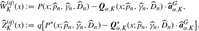 \begin{align*}\widehat{W}^{(q)}_{K}(x)&\;:\!=\; P(x;\;\widehat{p}_{n},\widehat{\gamma}_{n},\widehat{D}_{n}) -{\boldsymbol{Q}}_{\alpha,K}(x;\;\widehat{p}_{n},\widehat{\gamma}_{n},\widehat{D}_{n})\cdot \widehat{\boldsymbol{a}}^{G}_{\alpha,K}, \\[5pt] \widehat{Z}^{(q)}_{K}(x)&\;:\!=\; q \bigl[P^*(x;\;\widehat{p}_{n},\widehat{\gamma}_{n},\widehat{D}_{n}) -{\boldsymbol{Q}}^*_{\alpha,K}(x;\;\widehat{p}_{n},\widehat{\gamma}_{n},\widehat{D}_{n})\cdot \widehat{\boldsymbol{a}}^{G}_{\alpha,K}\bigr].\end{align*}
The consistency and asymptotic normality for $\widehat{W}^{(q)}_K$
are obtained for each
$\widehat{W}^{(q)}_K$
are obtained for each $K\in \mathbb{N}$
as follows.
$K\in \mathbb{N}$
as follows.
Theorem 3.1. Suppose the assumptions NPC, S1, S2, and M[2] hold. Then, for any $q>0$
,
$q>0$
, $K\in \mathbb{N}$
, and
$K\in \mathbb{N}$
, and $x \in \mathbb{R}_+$
, we have
$x \in \mathbb{R}_+$
, we have
 \begin{align*}\widehat{W}^{(q)}_K(x) \stackrel{p}{\to} W^{(q)}_K(x).\end{align*}
In particular, when $q=0$
, we have uniform consistency:
$q=0$
, we have uniform consistency:
 \begin{align*}\sup_{x\in\mathbb{R}_+}\bigl|\widehat{W}^{(0)}_K(x)-W^{(0)}_K(x)\bigr|\stackrel{p}{\to} 0.\end{align*}
In addition, suppose M[4] holds. Then we have
 \begin{align*}\sqrt{T_{n}}\bigl(\widehat{W}^{(q)}_{K}(x)-W^{(q)}_{K}(x)\bigr)\stackrel{d}{\to} N (0,\sigma_{K}(x)),\end{align*}
where $\sigma_{K}(x)\;:\!=\; [C_{K}(x)\Gamma_{K}]\Sigma_{K}[C_{K}(x)\Gamma_{K}]^{\top}$
with
$\sigma_{K}(x)\;:\!=\; [C_{K}(x)\Gamma_{K}]\Sigma_{K}[C_{K}(x)\Gamma_{K}]^{\top}$
with $\Sigma_{K}$
and
$\Sigma_{K}$
and $\Gamma_{K}$
given in (B.1) and (B.2), respectively, and
$\Gamma_{K}$
given in (B.1) and (B.2), respectively, and $C_K$
is the
$C_K$
is the $(2K+4)$
-dim vector given by
$(2K+4)$
-dim vector given by
 \begin{align*}&C_{K}(x)\;:\!=\; \\[5pt] &\ \bigl({\boldsymbol{Q}}_{\alpha,K}(x;\;p_0,\gamma_0,D_0)^\top \bigl(A_K^f\bigr)^{-1}B_{K},\partial_{(p,\gamma)}\bigl[P(x;\;\gamma_0,p_0,D_0)-{\boldsymbol{Q}}_{\alpha,K}(x;\;p_0,\gamma_0,D_0)\cdot \boldsymbol{a}^{G}_{\alpha,K}\bigr]\bigr)^\top ,\end{align*}
with the matrix $B_K$
given in Corollary B.1.
$B_K$
given in Corollary B.1.
Proof. See Section C.6.
Theorem 3.2. Suppose the assumptions NPC, S1, S2, and M[2] hold. Then, for any $q>0$
,
$q>0$
, $K\in \mathbb{N}$
, and
$K\in \mathbb{N}$
, and $x \in \mathbb{R}_+$
, we have
$x \in \mathbb{R}_+$
, we have
 \begin{align*}\widehat{Z}^{(q)}_K(x) \stackrel{p}{\to} Z^{(q)}_K(x).\end{align*}
In particular, when $q=0$
, we have uniform consistency: for any compact set
$q=0$
, we have uniform consistency: for any compact set $V\subset \mathbb{R}_+$
,
$V\subset \mathbb{R}_+$
,
 \begin{align*}\sup_{x\in V}\bigl|\widehat{Z}^{(0)}_K(x)-Z^{(0)}_K(x)\bigr|\stackrel{p}{\to} 0.\end{align*}
In addition, suppose M[4] holds. Then we have
 \begin{align*}\sqrt{T_{n}}\bigl(\widehat{Z}^{(q)}_K(x)-Z^{(q)}_K(x)\bigr)\stackrel{d}{\to} N\bigl(0,\sigma^*_{K}(x)\bigr),\end{align*}
where $\sigma^*_{K}(x)\;:\!=\; q^2[C^*_K(x)\Gamma_K]\Sigma_K[C^*_K(x)\Gamma_K]^\top$
with
$\sigma^*_{K}(x)\;:\!=\; q^2[C^*_K(x)\Gamma_K]\Sigma_K[C^*_K(x)\Gamma_K]^\top$
with $\Sigma_K$
and
$\Sigma_K$
and $\Gamma_K$
given in (B.1) and (B.2), respectively, and
$\Gamma_K$
given in (B.1) and (B.2), respectively, and $C^*_K$
is the
$C^*_K$
is the $(2K+4)$
-dim vector given by
$(2K+4)$
-dim vector given by
 \begin{align*}&C^*_K(x)\;:\!=\; \\[5pt] &\ \bigl({\boldsymbol{Q}}^*_{\alpha,K}(x;\;p_0,\gamma_0,D_0)^\top\bigl(A_K^f\bigr)^{-1}B_{K},\partial_{(p,\gamma)}\bigl[P^*(x;\;\gamma_0,p_0,D_0)-{\boldsymbol{Q}}^*_{\alpha,K}(x;\;p_0,\gamma_0,D_0)\cdot \boldsymbol{a}^{G}_{\alpha,K}\bigr]\bigr)^\top ,\end{align*}
with the matrix $B_K$
given in Corollary B.1.
$B_K$
given in Corollary B.1.
Proof. See Section C.7.
Corollary 3.1. Suppose the assumptions NPC, S1, S2, and M[2] hold. Then, for any $q>0$
,
$q>0$
, $K\in \mathbb{N}$
, and
$K\in \mathbb{N}$
, and $x \in \mathbb{R}_+$
, we have
$x \in \mathbb{R}_+$
, we have
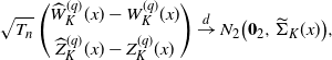 \begin{align*}\sqrt{T_{n}} \begin{pmatrix} \widehat{W}^{(q)}_{K}(x)-W^{(q)}_{K}(x)\\[5pt] \widehat{Z}^{(q)}_{K}(x)-Z^{(q)}_{K}(x) \end{pmatrix}\stackrel{d}{\to} N_{2}\bigl(\boldsymbol{0}_{2},\widetilde{\Sigma}_{K}(x)\bigr),\end{align*}
where
 \begin{align*}\widetilde{\Sigma}_{K}(x)\;:\!=\; \biggl[ \begin{pmatrix} C_{K}(x)\\[5pt] qC^{*}_{K}(x) \end{pmatrix}\Gamma_{K}\biggr]\Sigma_{K}\biggl[ \begin{pmatrix} C_{K}(x)\\[5pt] qC^{*}_{K}(x) \end{pmatrix}\Gamma_{K}\biggr]^{\top}.\end{align*}
Proof. See Section C.8.
Remark 3.2. Our asymptotic results for $\widehat{W}_K^{(q)}$
and
$\widehat{W}_K^{(q)}$
and $\widehat{Z}_K^{(q)}$
are all for a fixed
$\widehat{Z}_K^{(q)}$
are all for a fixed $K\in \mathbb{N}$
, and but one may also be concerned with the case where
$K\in \mathbb{N}$
, and but one may also be concerned with the case where $K=K_n\to \infty$
as well as
$K=K_n\to \infty$
as well as $n\to \infty$
. It is not a straightforward extension, even for consistency. For example, if we could show that for each
$n\to \infty$
. It is not a straightforward extension, even for consistency. For example, if we could show that for each $x\in \mathbb{R}_+$
,
$x\in \mathbb{R}_+$
,
 \begin{align*}\sup_{K\in \mathbb{N}}\bigl|\widehat{W}_K^{(q)}(x) - W_K^{(q)}(x)\bigr| \stackrel{p}{\to} 0,\quad n\to \infty,\end{align*}
then we can exchange the order of the limits $n\to \infty$
and
$n\to \infty$
and $K\to \infty$
, which concludes that
$K\to \infty$
, which concludes that $\widehat{W}_\infty^{(q)}(x) \stackrel{p}{\to} W_\infty^{(q)}(x)$
for each
$\widehat{W}_\infty^{(q)}(x) \stackrel{p}{\to} W_\infty^{(q)}(x)$
for each $x\in \mathbb{R}_+$
. On this point, we need further study. As for the extension of asymptotic normality, a more complicated discussion is needed to extend the results to the case where K depends on n with
$x\in \mathbb{R}_+$
. On this point, we need further study. As for the extension of asymptotic normality, a more complicated discussion is needed to extend the results to the case where K depends on n with $K=K_n\to \infty$
. This will lead to a high-dimensional setting, and we will need a high-dimensional central limit theorem (CLT) for triangular arrays, even without a martingale property. A sophisticated CLT would still need to be proved.
$K=K_n\to \infty$
. This will lead to a high-dimensional setting, and we will need a high-dimensional central limit theorem (CLT) for triangular arrays, even without a martingale property. A sophisticated CLT would still need to be proved.
Appendix A. Some auxiliary statistics
A.1. Estimator of
$\boldsymbol{D}_{\textbf{0}}$

For $D=\sigma^2/2$
, we consider the following estimator proposed by Jacod [Reference Jacod12] and Shimizu [Reference Shimizu22, Reference Shimizu23]: for each fixed
$D=\sigma^2/2$
, we consider the following estimator proposed by Jacod [Reference Jacod12] and Shimizu [Reference Shimizu22, Reference Shimizu23]: for each fixed $T>0$
,
$T>0$
,
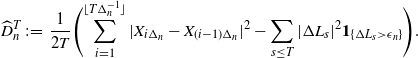 \begin{align*}\widehat{D}^{T}_{n}\;:\!=\; \dfrac{1}{2T}\Biggl(\sum_{i=1}^{\lfloor T\Delta_{n}^{-1}\rfloor}|X_{i\Delta_{n}}-X_{(i-1)\Delta_{n}}|^{2}-\sum_{s\le T}|\Delta L_{s}|^{2}\boldsymbol{1}_{\{\Delta L_{s}>{\epsilon}_n\}}\Biggr).\end{align*}
Lemma A.1. (Shimizu [Reference Shimizu22], Remark 3.2.) Under the assumptions S1 and S2, the estimator $\widehat{D}^T_n$
is consistent with
$\widehat{D}^T_n$
is consistent with $D_0$
with the rate of convergence being faster than
$D_0$
with the rate of convergence being faster than $\sqrt{T_n}$
such that for any
$\sqrt{T_n}$
such that for any $t>0$
,
$t>0$
,
 \begin{align*}\sqrt{T_n}\bigl(\widehat{D}^T_n - D_0\bigr) \stackrel{p}{\to} 0.\end{align*}
Remark A.1. Since the constant $T>0$
in the estimator
$T>0$
in the estimator $\widehat{D}^T_n$
can be arbitrary, we will fix it to be
$\widehat{D}^T_n$
can be arbitrary, we will fix it to be $T=1$
without loss of generality, and set
$T=1$
without loss of generality, and set
 \begin{align*}\widehat{D}_n \;:\!=\; \widehat{D}_n^1.\end{align*}
In practice, the value of T should be chosen appropriately based on the amount of data and the size of $\Delta_n$
.
$\Delta_n$
.
A.2. Estimator of
$\nu$
-functionals

First, we would like to estimate the integral-type functional $\nu (\boldsymbol{H}_\theta)$
, where
$\nu (\boldsymbol{H}_\theta)$
, where $\boldsymbol{H}_\theta\colon \mathbb{R}_+\to \mathbb{R}^d$
is a
$\boldsymbol{H}_\theta\colon \mathbb{R}_+\to \mathbb{R}^d$
is a $\nu$
-integrable function with an unknown parameter
$\nu$
-integrable function with an unknown parameter $\theta\in \Theta$
:
$\theta\in \Theta$
:
 \begin{align*}\nu(\boldsymbol{H}_\theta) \;:\!=\; \biggl( \int_0^\infty H_\theta^{(1)}(z)\,\nu(\mathrm{d} z), \ldots, \int_0^\infty H_\theta^{(d)}(z)\,\nu(\mathrm{d} z)\biggr),\end{align*}
where $\Theta$
is an open and bounded subset of
$\Theta$
is an open and bounded subset of $\mathbb{R}^l$
for some
$\mathbb{R}^l$
for some $l\in \mathbb{N}$
. Note that the parameter
$l\in \mathbb{N}$
. Note that the parameter $\theta$
can be a variety of parameters depending on the context. For instance, we will see later that the parameter
$\theta$
can be a variety of parameters depending on the context. For instance, we will see later that the parameter $p\;:\!=\; \int_0^\infty \widetilde{f}_q(z)\,\mathrm{d} z$
, the coefficients of Laguerre expansion, e.g.
$p\;:\!=\; \int_0^\infty \widetilde{f}_q(z)\,\mathrm{d} z$
, the coefficients of Laguerre expansion, e.g. $a_{\alpha,k}^f$
and
$a_{\alpha,k}^f$
and $a_{\alpha,k}^F$
, can all be expressed in terms of the integral functional of
$a_{\alpha,k}^F$
, can all be expressed in terms of the integral functional of $\nu$
.
$\nu$
.
In short, we need to estimate the parameters $(D_0,\gamma_0, \nu(\boldsymbol{H}_{\theta_0}))$
, where
$(D_0,\gamma_0, \nu(\boldsymbol{H}_{\theta_0}))$
, where $\theta_0$
is the true value of
$\theta_0$
is the true value of $\theta$
. Hereafter, we assume that there exists an open and bounded set
$\theta$
. Hereafter, we assume that there exists an open and bounded set $\Theta_1$
and
$\Theta_1$
and $\Theta_2$
of
$\Theta_2$
of $\mathbb{R}_+$
such that
$\mathbb{R}_+$
such that
 \begin{align*}(D_0,\gamma_0,\theta_0)\in \Theta_1\times \Theta_2.\end{align*}
Moreover, we make the following assumptions on an integrands $\boldsymbol{H}_\theta$
, which are applied to a variety of
$\boldsymbol{H}_\theta$
, which are applied to a variety of $\boldsymbol{H}_\theta$
, locally in this section.
$\boldsymbol{H}_\theta$
, locally in this section.
H1[ $\delta$
] For each
$\delta$
] For each $\theta\in \Theta$
, there exists a
$\theta\in \Theta$
, there exists a $\delta\ge 0$
such that
$\delta\ge 0$
such that $\nu(|\boldsymbol{H}_\theta| \vee|\boldsymbol{H}_\theta|^{2+\delta}) < \infty$
.
$\nu(|\boldsymbol{H}_\theta| \vee|\boldsymbol{H}_\theta|^{2+\delta}) < \infty$
.
H2 $\displaystyle \sup_{\theta \in \overline{\Theta}} \nu(|\boldsymbol{H}_\theta| \vee |\boldsymbol{H}_\theta|^2) < \infty$
.
$\displaystyle \sup_{\theta \in \overline{\Theta}} \nu(|\boldsymbol{H}_\theta| \vee |\boldsymbol{H}_\theta|^2) < \infty$
.
H3 There exists a $\nu$
-integrable function
$\nu$
-integrable function $h_1\colon \mathbb{R}_+\to \mathbb{R}$
such that
$h_1\colon \mathbb{R}_+\to \mathbb{R}$
such that
 \begin{align*}\sup_{\theta \in \overline{\Theta}} |\boldsymbol{H}_\theta(z)| \le h_1(z).\end{align*}
H4 There exists a function $h_2\colon \mathbb{R}_+\to \mathbb{R}$
with
$h_2\colon \mathbb{R}_+\to \mathbb{R}$
with $\nu\bigl(h_2\vee h_2^2\bigr) < \infty$
such that for any
$\nu\bigl(h_2\vee h_2^2\bigr) < \infty$
such that for any $\kappa \in \mathbb{R}^l$
,
$\kappa \in \mathbb{R}^l$
,
 \begin{align*}\sup_{\theta \in \overline{\Theta}} |\boldsymbol{H}_{\theta + \kappa}(z) - \boldsymbol{H}_\theta(z)| \le h_2(z)|\kappa|.\end{align*}
H5 For each $i=1,\ldots,d$
,
$i=1,\ldots,d$
,
 \begin{align*}\int_0^{{\epsilon}_n} H_\theta^{(i)}(z)\,\nu(\mathrm{d} z) = {\mathrm{o}} \bigl(T_n^{-1/2}\bigr).\end{align*}
As for functionals $\nu(\boldsymbol{H}_\theta)$
, we can use the following threshold-type estimator:
$\nu(\boldsymbol{H}_\theta)$
, we can use the following threshold-type estimator:
 \begin{align*}\widehat{\nu}_n(\boldsymbol{H}_\theta) \;:\!=\; \dfrac{1}{T_n} \sum_{t \in (0, T_n]} \boldsymbol{H}_\theta(\Delta L_t) \boldsymbol{1}_{\{\Delta L_t > {\epsilon}_n\}}.\end{align*}
Lemma A.2. (Shimizu [Reference Shimizu22], Propositions 3.1 and 3.2.)
-
(1) Under the assumption H1[0], we have
In addition, assuming further H2 and H4, we have uniform consistency:
\begin{align*}\widehat{\nu}_n(\boldsymbol{H}_\theta) \stackrel{p}{\to} \nu(\boldsymbol{H}_\theta),\quad \theta \in \Theta.\end{align*}
\begin{align*}\sup_{\theta \in \overline{\Theta}} |\widehat{\nu}_n(\boldsymbol{H}_\theta) - \nu(\boldsymbol{H}_\theta)| \to 0.\end{align*}
-
(2) Under H1[
$\delta$
] for some
$\delta>0$
and H5, we have where
\begin{align*}\sqrt{T_n}(\widehat{\nu}_n(\boldsymbol{H}_\theta) - \nu(\boldsymbol{H}_\theta)) \stackrel{d}{\to} N_d({\boldsymbol 0}_d,\Sigma_\theta), \quad \theta \in \Theta,\end{align*}
$\Sigma_\theta = \bigl(\nu\bigl(H_\theta^{(i)}H_\theta^{(j)}\bigr)\bigr)_{1\le i,j\le d}$
.


It will be easy to see that the following version of the continuous mapping-type theorem holds for the estimator $\widehat{\nu}_n(\boldsymbol{H}_\theta)$
.
$\widehat{\nu}_n(\boldsymbol{H}_\theta)$
.
Corollary A.1. Under the assumptions H1[0], H2–H4, it follows that
 \begin{align*}\widehat{\nu}_n\bigl(\boldsymbol{H}\boldsymbol{H}_{\widehat{\theta}_n}\bigr) \stackrel{p}{\to} \nu(\boldsymbol{H}_{\theta_0}),\end{align*}
for any random sequence such that $\widehat{\theta}_n \stackrel{p}{\to} \theta_0\in \Theta$
.
$\widehat{\theta}_n \stackrel{p}{\to} \theta_0\in \Theta$
.
Proof. Note that there exists a sub-subsequence $\{\widehat{\theta}_{n'}\}$
for any subsequence of
$\{\widehat{\theta}_{n'}\}$
for any subsequence of $\{\widehat{\theta}_n\}$
such that
$\{\widehat{\theta}_n\}$
such that $\widehat{\theta}_{n'} \to \theta_0$
a.s. Then, under the assumption H3, we can apply the Lebesgue-dominated convergence theorem to obtain
$\widehat{\theta}_{n'} \to \theta_0$
a.s. Then, under the assumption H3, we can apply the Lebesgue-dominated convergence theorem to obtain $\nu\bigl(\boldsymbol{H}_{\widehat{\theta}_{n'}}\bigr)\to\nu(\boldsymbol{H}_{\theta_0})$
a.s. That is, the sequence
$\nu\bigl(\boldsymbol{H}_{\widehat{\theta}_{n'}}\bigr)\to\nu(\boldsymbol{H}_{\theta_0})$
a.s. That is, the sequence $\bigl\{\nu\bigl(\boldsymbol{H}_{\widehat{\theta}_n}\bigr)\bigr\}$
has a sub-subsequence that converges to
$\bigl\{\nu\bigl(\boldsymbol{H}_{\widehat{\theta}_n}\bigr)\bigr\}$
has a sub-subsequence that converges to $\nu(\boldsymbol{H}_{\theta_0})$
almost surely, which implies that
$\nu(\boldsymbol{H}_{\theta_0})$
almost surely, which implies that $\nu\bigl(\boldsymbol{H}_{\widehat{\theta}_n}\bigr)\stackrel{p}{\to}\nu(\boldsymbol{H}_{\theta_0})$
. Moreover, since
$\nu\bigl(\boldsymbol{H}_{\widehat{\theta}_n}\bigr)\stackrel{p}{\to}\nu(\boldsymbol{H}_{\theta_0})$
. Moreover, since ${\mathbb{P}}(\widehat{\theta}_n\notin\Theta)\to 0$
, it follows from Lemma A.2 that for any
${\mathbb{P}}(\widehat{\theta}_n\notin\Theta)\to 0$
, it follows from Lemma A.2 that for any ${\epsilon}>0$
,
${\epsilon}>0$
,
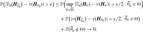 \begin{align*}{\mathbb{P}}\bigl(|\widehat{\nu}_{n}\bigl(\boldsymbol{H}_{\widehat{\theta}_n}\bigr)-\nu(\boldsymbol{H}_{\theta_0})|>{\epsilon}\bigr)&\le {\mathbb{P}}\Bigl(\sup_{\theta\in \overline{\Theta}} |\widehat{\nu}_{n}(\boldsymbol{H}_\theta)-\nu(\boldsymbol{H}_\theta)|>{\epsilon}/2,\ \widehat{\theta}_n\in\Theta\Bigr)\\[5pt] &\quad +{\mathbb{P}}\bigl(|\nu\bigl(\boldsymbol{H}_{\widehat{\theta}_n}\bigr)-\nu(\boldsymbol{H}_{\theta_0})|>{\epsilon}/2,\ \widehat{\theta}_n\in\Theta\bigr) \\[5pt] &\quad + {\mathbb{P}}(\widehat{\theta}_n\notin\Theta) \to 0.\end{align*}
This completes the proof.
A.3. Estimator of
$\gamma_0$

An estimator of the Lundberg exponent $\gamma_0 = \Phi(q)$
is found in Shimizu [Reference Shimizu22] as an M-estimator given by
$\gamma_0 = \Phi(q)$
is found in Shimizu [Reference Shimizu22] as an M-estimator given by
 \begin{align*}\widehat{\gamma}_n = \boldsymbol{1}_{\{q > 0\}}\cdot \arg\inf_{r \in \Theta_2}|c r + \widehat{D}_n r^2 - \widehat{\nu}_n(k_r) - q|^2,\end{align*}
where $k_r(z) = {\mathrm{e}}^{-r z} - 1$
. This estimator is quite natural because the contrast function is a direct estimator of the Lundberg equation ‘
$k_r(z) = {\mathrm{e}}^{-r z} - 1$
. This estimator is quite natural because the contrast function is a direct estimator of the Lundberg equation ‘ $\psi_X(r) - q =0$
’, and it is useful because it satisfies consistency and asymptotic normality, as follows.
$\psi_X(r) - q =0$
’, and it is useful because it satisfies consistency and asymptotic normality, as follows.
Lemma A.3 (Shimizu [Reference Shimizu22], Lemma 3.3.) Suppose the conditions NPC, S1, S2, and M[2] hold. Then we have
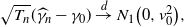 \begin{align*}\sqrt{T_n}(\widehat{\gamma}_n - \gamma_0) \stackrel{d}{\to} N_1\bigl(0,v_0^2\bigr),\end{align*}
where
 \begin{align*}v_0^2 = \dfrac{\nu\bigl(k_{\gamma_0}^2\bigr)}{ (c + 2D_0\gamma_0 + \nu(\partial_r k_{\gamma_0}))^2}.\end{align*}
In particular, we have the representation (in the proof of Lemma 3.3 of [Reference Shimizu22]) that
 \begin{align}\sqrt{T_n}(\widehat{\gamma}_n - \gamma_0) = \sqrt{T_n}(\widehat{\nu}_n(\widetilde{H}_{\gamma_0}) - \nu(\widetilde{H}_{\gamma_0})) + {\mathrm{o}}_p(1), \end{align}
where $\widetilde{H}_r(z)\;:\!=\; k_r(z) / \partial_z \psi_X(z)$
and
$\widetilde{H}_r(z)\;:\!=\; k_r(z) / \partial_z \psi_X(z)$
and $k_r(z) = {\mathrm{e}}^{-rz} - 1$
.
$k_r(z) = {\mathrm{e}}^{-rz} - 1$
.
Appendix B. Estimators of
$p_0$
,
$\boldsymbol{a}^f_{\alpha,K}$
,
$\boldsymbol{a}^F_{\alpha,K}$
, and
$\boldsymbol{a}^{G}_{\alpha,K}$


First, we prepare some notation to give representations of $p_0$
,
$p_0$
, $\boldsymbol{a}^f_{\alpha,K}$
, and
$\boldsymbol{a}^f_{\alpha,K}$
, and $\boldsymbol{a}^F_{\alpha,K}$
in terms of
$\boldsymbol{a}^F_{\alpha,K}$
in terms of $\nu$
-functionals.
$\nu$
-functionals.
Hereafter we set $\theta \;:\!=\; (D,\gamma) \in \overline{\Theta} \;:\!=\; \overline{\Theta}_1\times \overline{\Theta}_2$
, and let the true values be
$\theta \;:\!=\; (D,\gamma) \in \overline{\Theta} \;:\!=\; \overline{\Theta}_1\times \overline{\Theta}_2$
, and let the true values be
 \begin{align*}\theta_0 \;:\!=\; (D_0,\gamma_0) \in \Theta \;:\!=\; \Theta_1\times \Theta_2,\end{align*}
where $\Theta_1$
and
$\Theta_1$
and $\Theta_2$
are open and bounded subsets of
$\Theta_2$
are open and bounded subsets of $\mathbb{R}_+$
.
$\mathbb{R}_+$
.
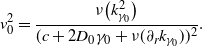
We define the following notation. As $D> 0$
, for
$D> 0$
, for $\alpha>0$
and
$\alpha>0$
and $k\in \mathbb{N}_0$
,
$k\in \mathbb{N}_0$
,
 \begin{align*}H_p(z;\;\theta) &\;:\!=\; D^{-1} \int_0^z \mathrm{d} y \int_y^\infty {\mathrm{e}}^{-\beta (x-y)}{\mathrm{e}}^{-\gamma (z-x)}\,\mathrm{d} x, \\[5pt] H_{\alpha,k}^f(z;\;\theta)&\;:\!=\; D^{-1}\int_0^z \,\mathrm{d} y \int_y^\infty {\mathrm{e}}^{-\beta (x-y)}{\mathrm{e}}^{-\gamma (z-x)}\varphi_{\alpha,k}(x)\,\mathrm{d} x, \\[5pt] H_{\alpha,k}^F(z;\;\theta)&\;:\!=\; D^{-1}\int_0^z \,\mathrm{d} y \int_y^\infty {\mathrm{e}}^{-\beta (x-y)}{\mathrm{e}}^{-\gamma (z-x)}\Psi_{\alpha,k}(x;\;0)\,\mathrm{d} x.\end{align*}
Recall that $\Psi_{\alpha,k}(x;\;b)$
is given by (2.10) in Definition 2.1. In particular, when
$\Psi_{\alpha,k}(x;\;b)$
is given by (2.10) in Definition 2.1. In particular, when $D=0$
,
$D=0$
,
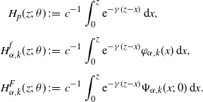 \begin{align*}H_p(z;\;\theta) &\;:\!=\; c^{-1}\int_0^z {\mathrm{e}}^{-\gamma (z-x)}\,\mathrm{d} x, \\[5pt] H_{\alpha,k}^f(z;\;\theta)&\;:\!=\; c^{-1}\int_0^z {\mathrm{e}}^{-\gamma (z-x)}\varphi_{\alpha,k}(x)\,\mathrm{d} x, \\[5pt] H_{\alpha,k}^F(z;\;\theta)&\;:\!=\; c^{-1}\int_0^z {\mathrm{e}}^{-\gamma (z-x)}\Psi_{\alpha,k}(x;\;0)\,\mathrm{d} x.\end{align*}
In this paper we use the convention
 \begin{align*}\boldsymbol{H}_{\alpha,K}^{f} = \bigl(H_{\alpha,0}^f, \ldots, H_{\alpha,K}^f\bigr)^\top.\end{align*}
Then it is straightforward to obtain the following expression by direct computation.
Lemma B.1. It holds that
 \begin{align*}p_0 = \nu(H_p(\cdot;\;\theta_0)),\quad a_{\alpha,k}^{f}= \nu\bigl(H_{\alpha,k}^f(\cdot;\;\theta_0)\bigr),\quad a_{\alpha,k}^F = \nu\bigl(H_{\alpha,k}^F(\cdot;\;\theta_0)\bigr).\end{align*}
Proof. Use Fubini’s theorem. We shall compute only $H_{\alpha,k}^F(z;\;\theta)$
:
$H_{\alpha,k}^F(z;\;\theta)$
:
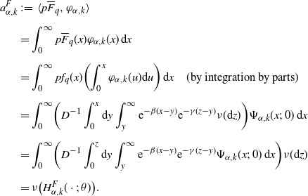 \begin{align*}a^{F}_{\alpha,k}&\;:\!=\; \langle p\overline{F}_{q},\varphi_{\alpha,k}\rangle\\[5pt] &=\int_{0}^{\infty}p\overline{F}_{q}(x)\varphi_{\alpha,k}(x)\,\mathrm{d} x\\[5pt] &=\int_{0}^{\infty}p f_{q}(x)\biggl(\int_{0}^{x}\varphi_{\alpha,k}(u)\mathrm{d}u\biggr)\,\mathrm{d} x \quad \mbox{(by integration by parts)}\\[5pt] &=\int_{0}^{\infty}\biggl(D^{-1}\int_{0}^{x}\mathrm{d}y\int_{y}^{\infty}{\mathrm{e}}^{-\beta(x-y)}{\mathrm{e}}^{-\gamma(z-y)}\nu(\mathrm{d}z)\biggr)\Psi_{\alpha,k}(x;\;0)\,\mathrm{d} x\\[5pt] &=\int_{0}^{\infty}\biggl(D^{-1}\int_{0}^{z}\mathrm{d}y\int_{y}^{\infty}{\mathrm{e}}^{-\beta(x-y)}{\mathrm{e}}^{-\gamma(z-y)}\Psi_{\alpha,k}(x;\;0)\,\mathrm{d} x\biggr)\nu(\mathrm{d}z)\\[5pt] &=\nu\bigl(H^{F}_{\alpha,k}(\cdot;\;\theta)\bigr).\end{align*}
The others are similar and omitted.
Thanks to this lemma, we have estimators of $p_0$
,
$p_0$
, $a^f_{\alpha,k}$
, and
$a^f_{\alpha,k}$
, and $a^F_{\alpha,k}$
as follows:
$a^F_{\alpha,k}$
as follows:
 \begin{align*}\widehat{p}_n = \widehat{\nu}_n(H_p(\cdot;\;\widehat{\theta}_n)),\quad \widehat{a}_{\alpha,k}^f = \widehat{\nu}_n\bigl(H_{\alpha,k}^f(\cdot;\;\widehat{\theta}_n)\bigr),\quad \widehat{a}_{\alpha,k}^F = \widehat{\nu}_n\bigl(H_{\alpha,k}^F(\cdot;\;\widehat{\theta}_n)\bigr),\end{align*}
where
 \begin{align*}\widehat{\theta}_n = (\widehat{D}_n, \widehat{\gamma}_n)^\top.\end{align*}
Theorem B.1. Suppose the assumptions NPC, S1, S2, and M[2] hold. Then the estimators $\widehat{p}_n$
,
$\widehat{p}_n$
, $ \widehat{a}_{\alpha,k}^f$
, and
$ \widehat{a}_{\alpha,k}^f$
, and $\widehat{a}_{\alpha,k}^F$
are consistent with their true values. In particular, it follows for each
$\widehat{a}_{\alpha,k}^F$
are consistent with their true values. In particular, it follows for each $\alpha>0$
and
$\alpha>0$
and $K\in \mathbb{N}$
that
$K\in \mathbb{N}$
that
 \begin{align*}\bigl(\widehat{\boldsymbol{a}}_{\alpha,K}^f, \widehat{\boldsymbol{a}}_{\alpha,K}^F,\widehat{p}_n\bigr)^\top \stackrel{p}{\to} \bigl(\boldsymbol{a}_{\alpha,K}^f, \boldsymbol{a}_{\alpha,K}^F,p_0\bigr)^\top,\end{align*}
where $p_0$
is the true value of
$p_0$
is the true value of $p=\int_0^\infty \widetilde{f}_q(z)\,\mathrm{d} z$
.
$p=\int_0^\infty \widetilde{f}_q(z)\,\mathrm{d} z$
.
Proof. According to Lemma B.1, $\widehat{p}_n$
,
$\widehat{p}_n$
, $\widehat{a}_{\alpha,k}^f$
, and
$\widehat{a}_{\alpha,k}^f$
, and $\widehat{a}_{\alpha,k}^F$
are all represented by
$\widehat{a}_{\alpha,k}^F$
are all represented by $\nu$
-functionals, for which we can apply Corollary A.1 since
$\nu$
-functionals, for which we can apply Corollary A.1 since $\widehat{\theta}_n = (\widehat{D}_n,\widehat{\gamma}_n) \stackrel{p}{\to} \theta_0=(D_0,\gamma_0)$
under our assumptions by Lemmas A.1 and A.3. Therefore we can check H1[0], H2–H4-type conditions for each
$\widehat{\theta}_n = (\widehat{D}_n,\widehat{\gamma}_n) \stackrel{p}{\to} \theta_0=(D_0,\gamma_0)$
under our assumptions by Lemmas A.1 and A.3. Therefore we can check H1[0], H2–H4-type conditions for each $H_\theta\;:\!=\; H_p$
,
$H_\theta\;:\!=\; H_p$
, $H_{\alpha,k}$
, and
$H_{\alpha,k}$
, and $H_{\alpha,k}^F$
, but it is straightforward under M[2] since H2 and H3 are true by Lemma C.3, and H4 is also true by Lemma C.4.
$H_{\alpha,k}^F$
, but it is straightforward under M[2] since H2 and H3 are true by Lemma C.3, and H4 is also true by Lemma C.4.
To state the asymptotic normality result, we define the following notation:
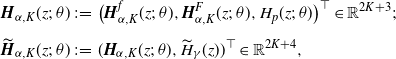 \begin{align*}\boldsymbol{H}_{\alpha,K}(z;\;\theta)&\;:\!=\; \bigl(\boldsymbol{H}^{f}_{\alpha,K}(z;\;\theta),\boldsymbol{H}^{F}_{\alpha,K}(z;\;\theta),H_{p}(z;\;\theta)\bigr)^{\top} \in \mathbb{R}^{2K+3}; \\[5pt] \widetilde{\boldsymbol{H}}_{\alpha,K}(z;\;\theta)&\;:\!=\; (\boldsymbol{H}_{\alpha,K}(z;\;\theta),\widetilde{H}_{\gamma}(z))^{\top} \in \mathbb{R}^{2K+4},\end{align*}
where $\widetilde{H}_\gamma$
is given in (A.1).
$\widetilde{H}_\gamma$
is given in (A.1).
Theorem B.2. Suppose the same assumptions as in Theorem B.1 and M[4] hold. Then we have asymptotic normality: for each $\alpha>0$
and
$\alpha>0$
and $K\in \mathbb{N}$
,
$K\in \mathbb{N}$
,
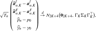 \begin{align*}\sqrt{T_n} \begin{pmatrix} \widehat{\boldsymbol{a}}^{f}_{\alpha,K}-\boldsymbol{a}^{f}_{\alpha,K}\\[5pt] \widehat{\boldsymbol{a}}^{F}_{\alpha,K}-\boldsymbol{a}^{F}_{\alpha,K}\\[5pt] \widehat{p}_{n}-p_0\\[5pt] \widehat{\gamma}_{n}-\gamma_0 \end{pmatrix}\stackrel{d}{\to} N_{2K+4}\bigl(\boldsymbol{0}_{2K+4},\Gamma_{K}\Sigma_{K}\Gamma_{K}^{\top}\bigr),\end{align*}
where $\Sigma_{K}\;:\!=\; (\sigma_{ij})_{1\leq i,j\leq 2K+4}$
with
$\Sigma_{K}\;:\!=\; (\sigma_{ij})_{1\leq i,j\leq 2K+4}$
with
 \begin{align}\sigma_{ij}\;:\!=\; \int_0^\infty \widetilde{H}_{\alpha,K}^{(i)}(z;\;\theta_0)\widetilde{H}_{\alpha,K}^{(j)}(z;\;\theta_0)\nu(\mathrm{d} z),\end{align}
and $\Gamma_{K}$
is the
$\Gamma_{K}$
is the $(2K+4)\times(2K+4)$
-matrix denoted by
$(2K+4)\times(2K+4)$
-matrix denoted by
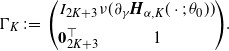 \begin{align}\Gamma_{K}\;:\!=\; \begin{pmatrix} I_{2K+3} & \nu(\partial_{\gamma}\boldsymbol{H}_{\alpha,K}(\cdot;\;\theta_0))\\[5pt] \boldsymbol{0}_{2K+3}^\top & 1 \end{pmatrix}\!.\end{align}
Proof. We only show the case where $D>0$
because the proof for
$D>0$
because the proof for $D=0$
is similar.
$D=0$
is similar.
Firstly, thanks to Taylor’s formula, it follows that
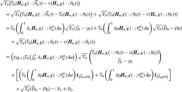 \begin{align*}&\sqrt{T_n}\bigl(\widehat{\nu}_{n}(\boldsymbol{H}_{\alpha,K}(\cdot;\;\widehat{\theta}_{n})) - \nu(\boldsymbol{H}_{\alpha,K}(\cdot;\;\theta_0))\bigr)\\[5pt] &\quad =\sqrt{T_n}\bigl(\widehat{\nu}_{n}(\boldsymbol{H}_{\alpha,K}(\cdot;\;\widehat{\theta}_{n}))-\widehat{\nu}_{n}(\boldsymbol{H}_{\alpha,K}(\cdot;\;\theta_0))\bigr) +\sqrt{T_n}(\widehat{\nu}_{n}(\boldsymbol{H}_{\alpha,K}(\cdot;\;\theta_0))-\nu(\boldsymbol{H}_{\alpha,K}(\cdot;\;\theta_0)))\\[5pt] &\quad =\widehat{\nu}_{n}\biggl(\int_0^{1}\partial_{\gamma}\boldsymbol{H}_{\alpha,K}(\cdot;\;\theta^{n}_{u})\,\mathrm{d} u\biggr)\sqrt{T_n}(\widehat{\gamma}_{n}-\gamma_0) +\widehat{\nu}_{n}\biggl(\int_0^{1}\partial_{D}\boldsymbol{H}_{\alpha,K}(\cdot;\;\theta^{n}_{u})\,\mathrm{d} u\biggr)\sqrt{T_n}(\widehat{D}_{n}-D_0)\\[5pt] &\qquad +\sqrt{T_n}(\widehat{\nu}_{n}(\boldsymbol{H}_{\alpha,K}(\cdot;\;\theta_0))-\nu(\boldsymbol{H}_{\alpha,K}(\cdot;\;\theta_0)))\\[5pt] &\quad =\begin{pmatrix} I_{2K+3} & \widehat{\nu}_{n}\bigl(\int_0^{1}\partial_{\gamma}\boldsymbol{H}_{\alpha,K}(\cdot;\;\theta^{n}_{u})\,\mathrm{d} u\bigr) \end{pmatrix} \sqrt{T_n} \begin{pmatrix} \widehat{\nu}_{n}(\boldsymbol{H}_{\alpha,K}(\cdot;\;\theta_0))-\nu(\boldsymbol{H}_{\alpha,K}(\cdot;\;\theta_0))\\[5pt] \widehat{\gamma}_{n}-\gamma_0 \end{pmatrix}\\[5pt] &\qquad +\biggl[ \biggl(\widehat{\nu}_{n}\biggl(\int_0^{1}\partial_{D}\boldsymbol{H}_{\alpha,K}(\cdot;\;\theta^{n}_{u})\,\mathrm{d} u\biggr)\boldsymbol{1}_{\{\widehat{\theta}_{n}\in\Theta\}}\biggr)+\widehat{\nu}_{n}\biggl(\int_0^{1}\partial_{D}\boldsymbol{H}_{\alpha,K}(\cdot;\;\theta^{n}_{u})\,\mathrm{d} u\biggr)\boldsymbol{1}_{\{\widehat{\theta}_{n}\notin\Theta\}} \biggr] \\[5pt] &\qquad\quad \times \sqrt{T_n}(\widehat{D}_{n}-D_0) =: S_{1}+S_{2},\end{align*}
where $\theta^{n}_{u}\;:\!=\; \theta_0+u(\widehat{\theta}_{n}-\theta_0)$
,
$\theta^{n}_{u}\;:\!=\; \theta_0+u(\widehat{\theta}_{n}-\theta_0)$
, $(u\in(0,1))$
.
$(u\in(0,1))$
.
As for $S_2$
, it follows from Lemma C.3 that for any
$S_2$
, it follows from Lemma C.3 that for any $k\in \mathbb{N}_0$
,
$k\in \mathbb{N}_0$
,
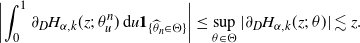 \begin{align*}\biggl|\int_0^{1}\partial_{D}H_{\alpha,k}(z;\;\theta^{n}_{u})\,\mathrm{d} u\boldsymbol{1}_{\{\widehat{\theta}_{n}\in\Theta\}}\biggr|\leq\sup_{\theta\in\Theta}|\partial_{D}H_{\alpha,k}(z;\;\theta)|\lesssim z.\end{align*}
Therefore the condition M[4] ensures that
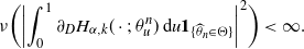 \begin{align*}\nu\biggl(\biggl|\int_0^{1}\partial_{D}H_{\alpha,k}(\cdot;\;\theta^{n}_{u})\,\mathrm{d} u\boldsymbol{1}_{\{\widehat{\theta}_{n}\in\Theta\}}\biggr|^{2}\biggr)<\infty.\end{align*}
Moreover, it follows for any ${\epsilon}>0$
that
${\epsilon}>0$
that
 \begin{align*}\biggl\{\widehat{\nu}_{n}\biggl(\int_0^{1}\partial_{D}\boldsymbol{H}_{\alpha,K}(\cdot;\;\theta^{n}_{u})\,\mathrm{d} u\biggr)\boldsymbol{1}_{\{\widehat{\theta}_{n}\notin\Theta\}}>{\epsilon}\biggr\}\subset\bigl\{\boldsymbol{1}_{\{\widehat{\theta}_{n}\notin\Theta\}}=1\bigr\}=\{\widehat{\theta}_{n}\notin\Theta\}.\end{align*}
Since $\widehat{\theta}_{n}\stackrel{p}{\to} \theta_0\in\Theta$
by S1, S2, and M[2], it follows from Lemmas A.1 and A.2 that
$\widehat{\theta}_{n}\stackrel{p}{\to} \theta_0\in\Theta$
by S1, S2, and M[2], it follows from Lemmas A.1 and A.2 that
 \begin{align*}S_2=({\mathrm{O}}_p(1)+{\mathrm{o}}_p(1))\sqrt{T_n}(\widehat{D}_n-D_0) \stackrel{p}{\to} 0.\end{align*}
Secondly, we show the following convergence:
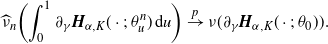 \begin{align}\widehat{\nu}_{n}\biggl(\int_0^{1}\partial_{\gamma}\boldsymbol{H}_{\alpha,K}(\cdot;\;\theta^{n}_{u})\,\mathrm{d} u\biggr)\stackrel{p}{\to} \nu(\partial_{\gamma}\boldsymbol{H}_{\alpha,K}(\cdot;\;\theta_0)). \end{align}
Thanks to Fubini’s theorem, we have
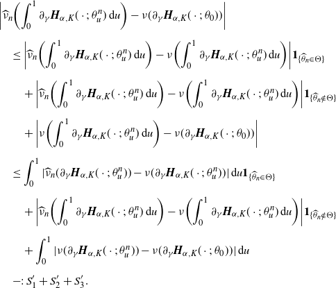 \begin{align*}&\biggl|\widehat{\nu}_{n}\biggl(\int_0^{1}\partial_{\gamma}\boldsymbol{H}_{\alpha,K}(\cdot;\;\theta^{n}_{u})\,\mathrm{d} u\biggr)-\nu(\partial_{\gamma}\boldsymbol{H}_{\alpha,K}(\cdot;\;\theta_0))\biggr|\\[5pt] &\quad \leq\biggl|\widehat{\nu}_{n}\biggl(\int_0^{1}\partial_{\gamma}\boldsymbol{H}_{\alpha,K}(\cdot;\;\theta^{n}_{u})\,\mathrm{d} u\biggr)-\nu\biggl(\int_0^{1}\partial_{\gamma}\boldsymbol{H}_{\alpha,K}(\cdot;\;\theta^{n}_{u})\,\mathrm{d} u\biggr)\biggr|\boldsymbol{1}_{\{\widehat{\theta}_{n}\in\Theta\}}\\[5pt] &\qquad +\biggl|\widehat{\nu}_{n}\biggl(\int_0^{1}\partial_{\gamma}\boldsymbol{H}_{\alpha,K}(\cdot;\;\theta^{n}_{u})\,\mathrm{d} u\biggr)-\nu\biggl(\int_0^{1}\partial_{\gamma}\boldsymbol{H}_{\alpha,K}(\cdot;\;\theta^{n}_{u})\,\mathrm{d} u\biggr)\biggr|\boldsymbol{1}_{\{\widehat{\theta}_{n}\notin\Theta\}}\\[5pt] &\qquad +\biggl|\nu\biggl(\int_0^{1}\partial_{\gamma}\boldsymbol{H}_{\alpha,K}(\cdot;\;\theta^{n}_{u})\,\mathrm{d} u\biggr)-\nu(\partial_{\gamma}\boldsymbol{H}_{\alpha,K}(\cdot;\;\theta_0))\biggr|\\[5pt] &\quad \leq\int_0^{1}|\widehat{\nu}_{n}(\partial_{\gamma}\boldsymbol{H}_{\alpha,K}(\cdot;\;\theta^{n}_{u}))-\nu(\partial_{\gamma}\boldsymbol{H}_{\alpha,K}(\cdot;\;\theta^{n}_{u}))|\,\mathrm{d} u\boldsymbol{1}_{\{\widehat{\theta}_{n}\in\Theta\}}\\[5pt] &\qquad +\biggl|\widehat{\nu}_{n}\biggl(\int_0^{1}\partial_{\gamma}\boldsymbol{H}_{\alpha,K}(\cdot;\;\theta^{n}_{u})\,\mathrm{d} u\biggr)-\nu\biggl(\int_0^{1}\partial_{\gamma}\boldsymbol{H}_{\alpha,K}(\cdot;\;\theta^{n}_{u})\,\mathrm{d} u\biggr)\biggr|\boldsymbol{1}_{\{\widehat{\theta}_{n}\notin\Theta\}}\\[5pt] &\qquad +\int_0^{1}|\nu(\partial_{\gamma}\boldsymbol{H}_{\alpha,K}(\cdot;\;\theta^{n}_{u}))-\nu(\partial_{\gamma}\boldsymbol{H}_{\alpha,K}(\cdot;\;\theta_0))|\,\mathrm{d} u\\[5pt] &\quad =: S'_{1}+S'_{2}+S'_{3}.\end{align*}
As for $S'_1$
, since
$S'_1$
, since
 \begin{align*}S'_1\leq\sup_{\theta\in\Theta}|\widehat{\nu}_{n}(\partial_{\gamma}\boldsymbol{H}_{\alpha,K}(\cdot;\;\theta))-\nu(\partial_{\gamma}\boldsymbol{H}_{\alpha,K}(\cdot;\;\theta))|,\end{align*}
we see from Lemmas A.2 and C.4 that $S'_1\stackrel{p}{\to} 0$
.
$S'_1\stackrel{p}{\to} 0$
.
As for $S'_2$
, since
$S'_2$
, since
 \begin{align*}\{|S'_{2}|>{\epsilon}' \} \subset\bigl\{\boldsymbol{1}_{\{\widehat{\theta}_{n}\notin\Theta\}}=1\bigr\}=\{\widehat{\theta}_{n}\notin\Theta\},\end{align*}
we have $S'_2\stackrel{p}{\to} 0$
by the consistency of
$S'_2\stackrel{p}{\to} 0$
by the consistency of $\widehat{\theta}_n$
.
$\widehat{\theta}_n$
.
As for $S'_3$
, note that
$S'_3$
, note that
 \begin{align*}S'_{3}&\leq\int_0^{1}|\nu(\partial_{\gamma}\boldsymbol{H}_{\alpha,k}(\cdot;\;\theta^{n}_{u}))-\nu(\partial_{\gamma}\boldsymbol{H}_{\alpha,k}(\cdot;\;\theta_0))|\boldsymbol{1}_{\{|\theta^{n}_{u}-\theta_0|<\delta'\}}\,\mathrm{d} u\\[5pt] &\quad +\int_0^{1}|\nu(\partial_{\gamma}\boldsymbol{H}_{\alpha,k}(\cdot;\;\theta^{n}_{u}))-\nu(\partial_{\gamma}\boldsymbol{H}_{\alpha,k}(\cdot;\;\theta_0))|\boldsymbol{1}_{\{|\theta^{n}_{u}-\theta_0|\geq\delta'\}}\,\mathrm{d} u.\end{align*}
The first term on the right-hand side goes to zero in probability due to the continuity of the mapping $\theta\mapsto\nu(\partial_{\gamma}\boldsymbol{H}_{\alpha,K}(\cdot;\;\theta))$
, which is a consequence by the Lebesgue convergence theorem with Lemma C.3 and the condition M[2]. The second term on the right-hand side also goes to zero in probability by the consistency of
$\theta\mapsto\nu(\partial_{\gamma}\boldsymbol{H}_{\alpha,K}(\cdot;\;\theta))$
, which is a consequence by the Lebesgue convergence theorem with Lemma C.3 and the condition M[2]. The second term on the right-hand side also goes to zero in probability by the consistency of $\theta_u^n$
to
$\theta_u^n$
to $\theta_0$
. Hence we see that
$\theta_0$
. Hence we see that $S'_{3}\stackrel{p}{\to} 0$
, which concludes the convergence (B.3).
$S'_{3}\stackrel{p}{\to} 0$
, which concludes the convergence (B.3).
Finally, we can show that
 \begin{align*}\sqrt{T_n}\bigl(\widehat{\nu}_{n}(\widetilde{\boldsymbol{H}}_{\alpha,K}(\cdot;\;\theta_0))-\nu(\widetilde{\boldsymbol{H}}_{\alpha,K}(\cdot;\;\theta_0))\bigr)\end{align*}
is asymptotically normal by checking the conditions in Lemma A.2 with $\boldsymbol{H}_\theta \;:\!=\; \widetilde{\boldsymbol{H}}_{\alpha,K}(\cdot;\;\theta)$
. In fact, it follows from Lemma C.3 and M[4] that
$\boldsymbol{H}_\theta \;:\!=\; \widetilde{\boldsymbol{H}}_{\alpha,K}(\cdot;\;\theta)$
. In fact, it follows from Lemma C.3 and M[4] that $\nu(|\boldsymbol{H}_\theta|^4) < \infty$
for each
$\nu(|\boldsymbol{H}_\theta|^4) < \infty$
for each $\theta\in \Theta$
, and that H5 also holds true since, by Lemma C.3 and (S2),
$\theta\in \Theta$
, and that H5 also holds true since, by Lemma C.3 and (S2),
 \begin{align*}&\int_0^{{\epsilon}_{n}}\bigl(H^{f}_{\alpha,k}(z;\;\theta)+H^{F}_{\alpha,k}(z;\;\theta)+H_{p}(z;\;\theta)+H_{\gamma_0}(z)\bigr)\nu(\mathrm{d} z)\\[5pt] &\quad \lesssim \int_0^{{\epsilon}_{n}}z\nu(\mathrm{d} z)\\[5pt] &\quad ={\mathrm{o}} \bigl(T_n^{-1/2}\bigr),\quad n\to\infty.\end{align*}
As a consequence, we see from Lemma A.2 that
 \begin{align*}\sqrt{T_n}(\widehat{\nu}_{n}(\widetilde{\boldsymbol{H}}_{\alpha,K}(\cdot;\;\theta_0))-\nu(\widetilde{\boldsymbol{H}}_{\alpha,K}(\cdot;\;\theta_0)))\stackrel{d}{\to} N_{2K+4}(\boldsymbol{0}_{2K+4},\Sigma_{K}),\end{align*}
where $\Sigma_K$
is given in (B.2). Now, putting
$\Sigma_K$
is given in (B.2). Now, putting
 \begin{align*}\widehat{\Gamma}_{K}\;:\!=\; \biggl( \begin{matrix} I_{2K+3} & \!\!\!\!\widehat{\nu}_{n}\bigl(\int_0^{1}\partial_{\gamma}\boldsymbol{H}_{\alpha,K}(\ \cdot\ \colon \theta_0)\,\mathrm{d} u\bigr)\\[5pt] \boldsymbol{0}_{2K+3} & 1 \end{matrix}\biggr),\end{align*}
we have the expression
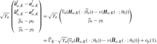 \begin{align*}\sqrt{T_n} \begin{pmatrix} \widehat{\boldsymbol{a}}^{f}_{\alpha,K}-\boldsymbol{a}^{f}_{\alpha,K}\\[5pt] \widehat{\boldsymbol{a}}^{F}_{\alpha,K}-\boldsymbol{a}^{F}_{\alpha,K}\\[5pt] \widehat{p}_{n}-p_0\\[5pt] \widehat{\gamma}_{n}-\gamma_0 \end{pmatrix}&=\sqrt{T_n} \begin{pmatrix} \widehat{\nu}_{n}(\boldsymbol{H}_{\alpha,K}(\cdot;\widehat{\theta}_{n}))-\nu(\boldsymbol{H}_{\alpha,K}(\cdot;\;\theta_0))\\[5pt] \widehat{\gamma}_{n}-\gamma_0 \end{pmatrix}\\[5pt] &=\widehat{\Gamma}_{K}\cdot\sqrt{T_n}\bigl(\widehat{\nu}_{n}(\widetilde{\boldsymbol{H}}_{\alpha,K}(\cdot;\;\theta_0))-\nu(\widetilde{\boldsymbol{H}}_{\alpha,K}(\cdot;\;\theta_0))\bigr)+{\mathrm{o}}_{p}(1).\end{align*}
Since $\widehat{\Gamma}_K\stackrel{p}{\to} \Gamma_K$
by (B.3), Slutsky’s lemma yields the result, and the proof is completed.
$\widehat{\Gamma}_K\stackrel{p}{\to} \Gamma_K$
by (B.3), Slutsky’s lemma yields the result, and the proof is completed.
According to Shimizu and Zhang [Reference Shimizu and Zhimin24], Theorems 1 and 2 and their proofs, we find the following results.
Corollary B.1. Under the same assumptions as in Theorem B.1, it holds that
 \begin{align*}\widehat{\boldsymbol{a}}^{G}_{\alpha,K}\stackrel{p}{\to} \boldsymbol{a}^{G}_{\alpha,K}.\end{align*}
In addition, suppose M[2] holds. Then $\widehat{\boldsymbol{a}}^{G}_{\alpha,K}$
is asymptotically normal since
$\widehat{\boldsymbol{a}}^{G}_{\alpha,K}$
is asymptotically normal since
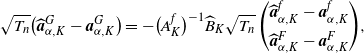 \begin{equation}\sqrt{T_{n}}\bigl(\widehat{\boldsymbol{a}}^{G}_{\alpha,K}-\boldsymbol{a}^{G}_{\alpha,K}\bigr)=-\bigl(A_K^f\bigr)^{-1}\widehat{B}_{K}\sqrt{T_{n}} \begin{pmatrix} \widehat{\boldsymbol{a}}^{f}_{\alpha,K}-\boldsymbol{a}^{f}_{\alpha,K}\\[5pt] \widehat{\boldsymbol{a}}^{F}_{\alpha,K}-\boldsymbol{a}^{F}_{\alpha,K} \end{pmatrix}\!,\end{equation}
where $\widehat{B}_K$
is a consistent estimator of the the
$\widehat{B}_K$
is a consistent estimator of the the $(K+1)\times(2K+2)$
matrix
$(K+1)\times(2K+2)$
matrix $B_K$
given as follows:
$B_K$
given as follows: $B_K \;:\!=\; (B^{*}_{K}, -I_{K+1})$
, where
$B_K \;:\!=\; (B^{*}_{K}, -I_{K+1})$
, where $B^{*}_{K}\;:\!=\; (b_{kl})_{1\leq k,l\leq K+1}$
, whose elements are given by
$B^{*}_{K}\;:\!=\; (b_{kl})_{1\leq k,l\leq K+1}$
, whose elements are given by
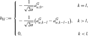 \begin{align*}b_{kl}\;:\!=\; \left\{ \begin{aligned} & -\dfrac{1}{\sqrt{2\alpha}}a^{G}_{\alpha,0}, & k=l,\\[5pt] & -\dfrac{1}{\sqrt{2\alpha}}\bigl(a^{G}_{\alpha,k-l}-a^{G}_{\alpha,k-l-1}\bigr), & k>l,\\[5pt] & 0, & k<l. \end{aligned}\right.\end{align*}
For example, an estimator $\widehat{B}_K$
is obtained by replacing
$\widehat{B}_K$
is obtained by replacing $a^{G}_{\alpha,k}$
, each element of
$a^{G}_{\alpha,k}$
, each element of $B_K$
, by its consistent estimator
$B_K$
, by its consistent estimator $\widehat{a}^{G}_{\alpha,k}$
.
$\widehat{a}^{G}_{\alpha,k}$
.
Appendix C. Auxiliary lemmas and some proofs
C.1. On functions
$\boldsymbol{f}_{\boldsymbol{q}}$
,
$\boldsymbol{F}_{\boldsymbol{q}}$
, and
$\boldsymbol{G}_{\boldsymbol{q}}$


Lemma C.1 Under the NPC condition, the probability density $f_q$
is well-defined and uniformly bounded.
$f_q$
is well-defined and uniformly bounded.
Proof. We prove only the case where $D>0$
, and the one for
$D>0$
, and the one for $D=0$
is similarly proved. First, we see from Lemma 3.2 in Feng and Shimizu [Reference Feng and Shimizu9] that
$D=0$
is similarly proved. First, we see from Lemma 3.2 in Feng and Shimizu [Reference Feng and Shimizu9] that
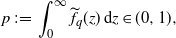 \begin{align*}p\;:\!=\; \int_0^\infty \widetilde{f}_q(z)\,\mathrm{d} z \in (0,1),\end{align*}
under the net profit condition NPC. Therefore $f_q\;:\!=\; p^{-1}\widetilde{f}_q$
is well-defined.
$f_q\;:\!=\; p^{-1}\widetilde{f}_q$
is well-defined.
Moreover, since ${\mathrm{e}}^{-\gamma(z-y)}<1$
for
${\mathrm{e}}^{-\gamma(z-y)}<1$
for $y<z<\infty$
and
$y<z<\infty$
and ${\mathrm{e}}^{-\beta(x-y)}\le 1$
for
${\mathrm{e}}^{-\beta(x-y)}\le 1$
for $0<x\le y$
, it follows that
$0<x\le y$
, it follows that $f_q$
is uniformly bounded as follows: for any
$f_q$
is uniformly bounded as follows: for any $x\in \mathbb{R}$
,
$x\in \mathbb{R}$
,
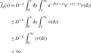 \begin{align*}\widetilde{f}_{q}(x)&=D^{-1}\int_{0}^{x}\mathrm{d} y\int_{y}^{\infty}{\mathrm{e}}^{-\beta(x-y)}{\mathrm{e}}^{-\gamma(z-y)}\nu(\mathrm{d} z) \\[5pt] &\le D^{-1}\int_{0}^{x}\mathrm{d} y\int_{y}^{\infty}\nu(\mathrm{d} z) \\[5pt] &\le D^{-1}\int_{0}^{\infty}z\nu(\mathrm{d} z) \\[5pt] &< \infty.\end{align*}
Lemma C.2. For $F_{q}$
and
$F_{q}$
and $G_{q}$
, their tail functions satisfy that
$G_{q}$
, their tail functions satisfy that $\overline{F}_{q}, \overline{G}_{q}\in L^s(\mathbb{R}_{+})$
for any
$\overline{F}_{q}, \overline{G}_{q}\in L^s(\mathbb{R}_{+})$
for any $s\ge 1$
.
$s\ge 1$
.
Proof. Since $0\le \overline{F}_{q}(x), \overline{G}_{q}(x)\le 1$
for any
$0\le \overline{F}_{q}(x), \overline{G}_{q}(x)\le 1$
for any $x\in \mathbb{R}$
, it suffices to show that
$x\in \mathbb{R}$
, it suffices to show that $\overline{F}_{q}, \overline{G}_{q}\in L^{1}(\mathbb{R}_{+})$
. The Fubini theorem yields that
$\overline{F}_{q}, \overline{G}_{q}\in L^{1}(\mathbb{R}_{+})$
. The Fubini theorem yields that
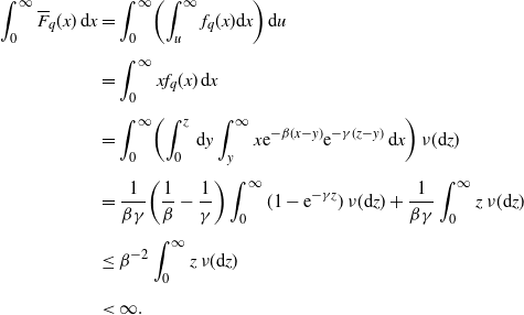 \begin{align*}\int_{0}^{\infty}\overline{F}_{q}(x)\,\mathrm{d} x&=\int_{0}^{\infty}\biggl(\int_{u}^{\infty}f_{q}(x)\mathrm{d} x\biggr)\,\mathrm{d} u \\[5pt] &=\int_{0}^{\infty}xf_{q}(x)\,\mathrm{d} x\\[5pt] &=\int_{0}^{\infty}\biggl(\int_{0}^{z}\,\mathrm{d} y\int_{y}^{\infty}x{\mathrm{e}}^{-\beta(x-y)}{\mathrm{e}}^{-\gamma(z-y)}\,\mathrm{d} x\biggr)\,\nu(\mathrm{d} z)\\[5pt] &=\dfrac{1}{\beta\gamma}\biggl(\dfrac{1}{\beta}-\dfrac{1}{\gamma}\biggr)\int_{0}^{\infty}(1-{\mathrm{e}}^{-\gamma z})\,\nu(\mathrm{d} z)+\dfrac{1}{\beta\gamma}\int_{0}^{\infty}z\,\nu(\mathrm{d} z)\\[5pt] &\le\beta^{-2}\int_{0}^{\infty}z\,\nu(\mathrm{d} z)\\[5pt] &<\infty.\end{align*}
Moreover, taking the Laplace transform of the DRE (2.4) for $G_q$
, we have
$G_q$
, we have
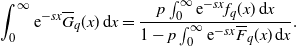 \begin{align*}\int_{0}^{\infty}{\mathrm{e}}^{-sx}\overline{G}_{q}(x)\,\mathrm{d} x=\dfrac{p\int_{0}^{\infty}{\mathrm{e}}^{-sx}f_{q}(x)\,\mathrm{d} x}{1-p\int_{0}^{\infty}{\mathrm{e}}^{-sx}\overline{F}_{q}(x)\,\mathrm{d} x}.\end{align*}
Substituting with $s=0$
, we have
$s=0$
, we have $\overline{G}_{q}\in L^{1}(\mathbb{R}_{+})$
since
$\overline{G}_{q}\in L^{1}(\mathbb{R}_{+})$
since $f_{q},\overline{F}_{q}\in L^{1}(\mathbb{R}_{+})$
.
$f_{q},\overline{F}_{q}\in L^{1}(\mathbb{R}_{+})$
.
C.2. On functions
$\boldsymbol{H}_{\boldsymbol{p}}$
,
$\boldsymbol{H}_{\boldsymbol\alpha,\boldsymbol{k}}^{\boldsymbol{f}}$
, and
$\boldsymbol{H}_{\boldsymbol\alpha,\boldsymbol{k}}^{\boldsymbol{F}}$


Lemma C.3. For each $z\in \mathbb{R}_{+}$
and
$z\in \mathbb{R}_{+}$
and $m=0, 1$
, the following inequalities hold true:
$m=0, 1$
, the following inequalities hold true:
 \begin{align*}\sup_{\theta\in \overline{\Theta}}|\partial_{D}^{m}H_{p}(z;\;\theta) | \lesssim z,\quad\sup_{\theta\in \overline{\Theta}}|\partial_{D}^{m}H^{f}_{\alpha,k}(z;\;\theta)| \lesssim z,\quad\sup_{\theta\in \overline{\Theta}}|\partial_{D}^{m}H^{F}_{\alpha,k}(z;\;\theta)| \lesssim z.\end{align*}
Moreover, it follows that
 \begin{align*}\sup_{\theta\in \overline{\Theta}}|\partial_{\gamma}H_{p}(z;\;\theta)| \lesssim z,\quad\sup_{\theta\in \overline{\Theta}}|\partial_{\gamma}H^{f}_{\alpha,k}(z;\;\theta)| \lesssim z,\quad\sup_{\theta\in \overline{\Theta}}|\partial_{\gamma}H^{F}_{\alpha,k}(z;\;\theta)| \lesssim z + z^2.\end{align*}
Proof. We shall show the case where $D>0$
. The case where
$D>0$
. The case where $D=0$
is similarly proved. Since
$D=0$
is similarly proved. Since $\Theta=\Theta_1\times \Theta_2$
, each
$\Theta=\Theta_1\times \Theta_2$
, each $\Theta_i$
is open and bounded, we can assume that
$\Theta_i$
is open and bounded, we can assume that
 \begin{align*}\Theta=\bigl(\eta_{1},\eta_{1}^{-1}\bigr)\times\bigl(\eta_{2},\eta_{2}^{-1}\bigr),\end{align*}
for $\eta_{1},\eta_{2}>0$
small enough without loss of generality. Then we have
$\eta_{1},\eta_{2}>0$
small enough without loss of generality. Then we have
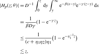 \begin{align*}|H_{p}(z;\;\theta)|&= D^{-1}\int_{0}^{z}\,\mathrm{d} y\int_{y}^{\infty}{\mathrm{e}}^{-\beta(x-y)}{\mathrm{e}}^{-\gamma(z-y)}\,\mathrm{d} x \\[5pt] &=\dfrac{1}{\beta D\gamma}(1-{\mathrm{e}}^{-\gamma z}) \\[5pt] &\le\dfrac{1}{(c+\eta_{1}\eta_{2})\eta_{1}}\bigl(1-{\mathrm{e}}^{-\eta_{1}^{-1} z}\bigr) \\[5pt] &\lesssim z,\end{align*}
uniformly in $\theta \in \overline{\Theta}$
. Then, due to (2.2), we see that
$\theta \in \overline{\Theta}$
. Then, due to (2.2), we see that $|H^{f}_{\alpha,k}(z;\;\theta)|\le\sqrt{2\alpha}|H_{p}(z;\;\theta)|$
, which yields
$|H^{f}_{\alpha,k}(z;\;\theta)|\le\sqrt{2\alpha}|H_{p}(z;\;\theta)|$
, which yields $\sup_{\theta\in \overline{\Theta}}|H^{f}_{\alpha,k}(z;\;\theta)|\lesssim z$
. Moreover, since it also holds that
$\sup_{\theta\in \overline{\Theta}}|H^{f}_{\alpha,k}(z;\;\theta)|\lesssim z$
. Moreover, since it also holds that $\sup_{k\in\mathbb{N}_{0}}|\Phi_{\alpha,k}(x;\;0)|\le \sqrt{2\alpha}x$
, we have
$\sup_{k\in\mathbb{N}_{0}}|\Phi_{\alpha,k}(x;\;0)|\le \sqrt{2\alpha}x$
, we have
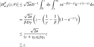 \begin{align*}\bigl|H^{F}_{\alpha,k}(z;\;\theta)\bigr|&\le\sqrt{2\alpha}D^{-1}\int_{0}^{z}\,\mathrm{d} y\int_{y}^{\infty}x{\mathrm{e}}^{-\beta(x-y)}{\mathrm{e}}^{-\gamma(z-y)}\,\mathrm{d} x \\[5pt] &=\dfrac{\sqrt{2\alpha}}{\beta D\gamma}\biggl(z-\biggl(\dfrac{1}{\gamma}-\dfrac{1}{\beta}\biggr)(1-{\mathrm{e}}^{-\gamma z})\biggr) \\[5pt] &\le\dfrac{\sqrt{2\alpha}}{(c+\eta_{1}\eta_{2})\eta_{1}}z\\[5pt] &\lesssim z.\end{align*}
Other proofs can be done similarly, so we omit them and end here.
Lemma C.4. For each $z\in \mathbb{R}_+$
,
$z\in \mathbb{R}_+$
, $m=0, 1$
, and
$m=0, 1$
, and $\kappa>0$
, the following inequalities hold true:
$\kappa>0$
, the following inequalities hold true:
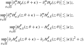 \begin{align*}\sup_{\theta\in \overline{\Theta}}\bigl|\partial_{\gamma}^{m}H_{p}(z;\;\theta+\kappa)-\partial_{\gamma}^{m}H_{p}(z;\;\theta)\bigr|&\lesssim |\kappa| z,\\[5pt] \sup_{\theta\in \overline{\Theta}}\bigl|\partial_{\gamma}^{m}H^{f}_{\alpha,k}(z;\;\theta+\kappa)-\partial_{\gamma}^{m}H^{f}_{\alpha,k}(z;\;\theta)\bigr|&\lesssim |\kappa|z,\\[5pt] \sup_{\theta\in \overline{\Theta}}\bigl|H^{F}_{\alpha,k}(z;\;\theta+\kappa)-H^{F}_{\alpha,k}(z;\;\theta)\bigr|&\lesssim |\kappa|z,\\[5pt] \sup_{\theta\in \overline{\Theta}}\bigl|\partial_{\gamma}H^{F}_{\alpha,k}(z;\;\theta+\kappa)-\partial_{\gamma}H^{F}_{\alpha,k}(z;\;\theta)\bigr| &\lesssim |\kappa|(z^{2}+z).\end{align*}
Proof. We shall show the case where $D>0$
. The case where
$D>0$
. The case where $D=0$
is similarly proved. As in the previous proof, we assume that
$D=0$
is similarly proved. As in the previous proof, we assume that $\Theta=\bigl(\eta_{1},\eta_{1}^{-1}\bigr)\times\bigl(\eta_{2},\eta_{2}^{-1}\bigr)$
for
$\Theta=\bigl(\eta_{1},\eta_{1}^{-1}\bigr)\times\bigl(\eta_{2},\eta_{2}^{-1}\bigr)$
for $\eta_{1},\eta_{2}>0$
small enough without loss of generality, and put
$\eta_{1},\eta_{2}>0$
small enough without loss of generality, and put $\kappa\;:\!=\; (\kappa_{1},\kappa_{2})^{\top}$
.
$\kappa\;:\!=\; (\kappa_{1},\kappa_{2})^{\top}$
.
Let
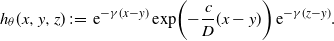 \begin{align*}h_{\theta}(x,y,z)\;:\!=\; {\mathrm{e}}^{-\gamma(x-y)} \exp\biggl({-\frac{c}{D}(x-y)}\biggr)\,{\mathrm{e}}^{-\gamma(z-y)}.\end{align*}
Note that it follows for $y<x<\infty$
,
$y<x<\infty$
, $0<y\le z$
that
$0<y\le z$
that
 \begin{align}\biggl|\exp\biggl(\!-\!\frac{c}{D+\kappa_{2}}(x-y)\biggr)-\exp\biggl(\!-\!\frac{c}{D}(x-y)\biggr)\biggr| \,{\mathrm{e}}^{-\gamma(z-y)}\ge |h_{\theta+\kappa}(x,y,z)-h_{\theta}(x,y,z)|. \end{align}
Using this inequality, we have
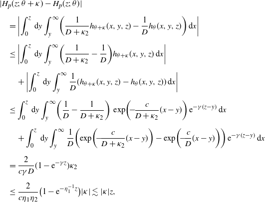 \begin{align*}&|H_{p}(z;\;\theta+\kappa)-H_{p}(z;\;\theta)|\\[5pt] &\quad =\biggl|\int_0^{z}\,\mathrm{d} y\int_{y}^\infty \biggl(\dfrac{1}{D+\kappa_{2}}h_{\theta+\kappa}(x,y,z)-\dfrac{1}{D}h_{\theta}(x,y,z)\biggr)\,\mathrm{d} x\biggr|\\[5pt] &\quad \le\biggl|\int_0^{z}\,\mathrm{d} y\int_{y}^\infty \biggl(\dfrac{1}{D+\kappa_{2}}-\dfrac{1}{D}\biggr)h_{\theta+\kappa}(x,y,z)\,\mathrm{d} x\biggr| \\[5pt] &\quad \quad +\biggl|\int_0^{z}\,\mathrm{d} y\int_{y}^\infty \dfrac{1}{D}(h_{\theta+\kappa}(x,y,z)-h_{\theta}(x,y,z))\,\mathrm{d} x\biggr| \\[5pt] &\quad \le\int_0^{z}\,\mathrm{d} y\int_{y}^\infty \biggl(\dfrac{1}{D}-\dfrac{1}{D+\kappa_{2}}\biggr)\,\exp\biggl(\!-\!\frac{c}{D+\kappa_{2}}(x-y)\biggr)\,{\mathrm{e}}^{-\gamma(z-y)}\,\mathrm{d} x \\[5pt] &\quad \quad +\int_0^{z}\,\mathrm{d} y\int_{y}^\infty \dfrac{1}{D}\biggl(\exp\biggl(\!-\!\frac{c}{D+\kappa_{2}}(x-y)\biggr)-\exp\biggl(\!-\!\frac{c}{D}(x-y)\biggr)\biggr)\,{\mathrm{e}}^{-\gamma(z-y)}\,\mathrm{d} x\\[5pt] &\quad =\dfrac{2}{c\gamma D}(1-{\mathrm{e}}^{-\gamma z})\kappa_{2} \\[5pt] &\quad \le\dfrac{2}{c\eta_{1}\eta_{2}}\bigl(1-{\mathrm{e}}^{-\eta_{1}^{-1} z}\bigr)|\kappa| \lesssim |\kappa|z,\end{align*}
uniformly in $\theta \in \overline{\Theta}$
.
$\theta \in \overline{\Theta}$
.
As for $H_{\alpha,k}^f$
, since
$H_{\alpha,k}^f$
, since
 \begin{align*}\bigl|H^{f}_{\alpha,k}(z;\;\theta+\kappa)-H^{f}_{\alpha,k}(z;\;\theta)\bigr|\le\sqrt{2\alpha}|H_{p}(z;\;\theta+\kappa)-H_{p}(z;\;\theta)|\end{align*}
by (2.2), we obtain that
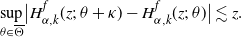 \begin{align*}\sup_{\theta\in \overline{\Theta}}\bigl|H^{f}_{\alpha,k}(z;\;\theta+\kappa)-H^{f}_{\alpha,k}(z;\;\theta)\bigr|\lesssim z.\end{align*}
Similarly, from (2.2) and (C.1), we have
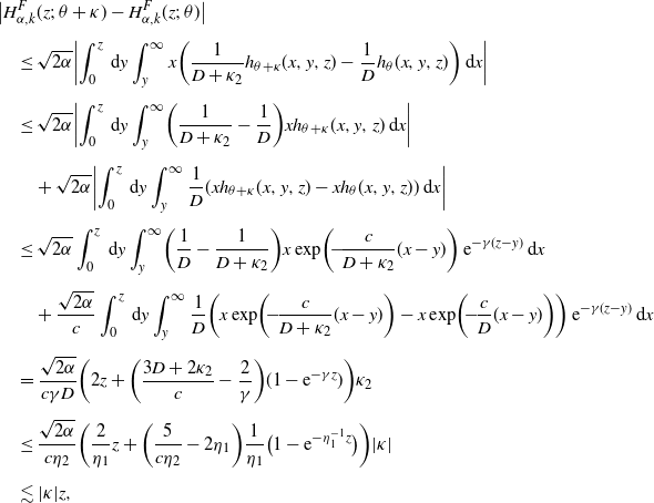 \begin{align*}&\big|H^{F}_{\alpha,k}(z;\;\theta+\kappa) - H^{F}_{\alpha,k}(z;\;\theta)\big|\\[5pt] &\quad \le\sqrt{2\alpha}\biggl|\int_0^{z}\,\mathrm{d} y\int_{y}^\infty x\biggl(\dfrac{1}{D+\kappa_{2}}h_{\theta+\kappa}(x,y,z)-\dfrac{1}{D}h_{\theta}(x,y,z)\biggr)\,\mathrm{d} x\biggr|\\[5pt] &\quad \le\sqrt{2\alpha}\biggl|\int_0^{z}\,\mathrm{d} y\int_{y}^\infty\biggl(\dfrac{1}{D+\kappa_{2}}-\dfrac{1}{D}\biggr)xh_{\theta+\kappa}(x,y,z)\,\mathrm{d} x\biggr|\\[5pt] &\qquad +{\sqrt{2\alpha}}\biggl|\int_0^{z}\,\mathrm{d} y\int_{y}^\infty\dfrac{1}{D}(xh_{\theta+\kappa}(x,y,z)-xh_{\theta}(x,y,z))\,\mathrm{d} x\biggr|\\[5pt] &\quad \le\sqrt{2\alpha}\int_0^{z}\,\mathrm{d} y\int_{y}^\infty\biggl(\dfrac{1}{D}-\dfrac{1}{D+\kappa_{2}}\biggr)x \exp\biggl(\!-\!\frac{c}{D+\kappa_{2}}(x-y)\biggr)\,{\mathrm{e}}^{-\gamma (z-y)}\,\mathrm{d} x\\[5pt] &\qquad +\dfrac{\sqrt{2\alpha}}{c}\int_0^{z}\,\mathrm{d} y\int_{y}^\infty\dfrac{1}{D}\biggl(x\exp\biggl(\!-\!\frac{c}{D+\kappa_{2}}(x-y)\biggr)-x \exp\biggl(\!-\!\frac{c}{D}(x-y)\biggr)\biggr) \,{\mathrm{e}}^{-\gamma (z-y)}\,\mathrm{d} x\\[5pt] &\quad =\dfrac{\sqrt{2\alpha}}{c\gamma D}\biggl(2z+\biggl(\dfrac{3D+2\kappa_{2}}{c}-\dfrac{2}{\gamma}\biggr)(1-{\mathrm{e}}^{-\gamma z})\biggr)\kappa_{2} \\[5pt] &\quad \le\dfrac{\sqrt{2\alpha}}{c\eta_{2}}\biggl(\dfrac{2}{\eta_{1}}z+\biggl(\dfrac{5}{c\eta_{2}}-2\eta_{1}\biggr)\dfrac{1}{\eta_{1}}\bigl(1-{\mathrm{e}}^{-\eta_{1}^{-1} z}\bigr)\biggr)|\kappa| \\[5pt] &\quad \lesssim |\kappa|z,\end{align*}
uniformly in $\theta \in \overline{\Theta}$
.
$\theta \in \overline{\Theta}$
.
Other proofs can be done similarly, so we omit them and end here.
C.3. On functions P,
$\boldsymbol{Q}_{\boldsymbol\alpha,\boldsymbol{k}}$
,
$\boldsymbol{P}^{\boldsymbol\ast}$
, and
$\boldsymbol{Q}^{\boldsymbol\ast}_{\boldsymbol\alpha,\boldsymbol{k}}$


Lemma C.5. The following statements are true.
-
(a) For each
$x\in \mathbb{R}$
, the mappings are of
\begin{align*} (p,\gamma,D)\mapsto P(x;\;p,\gamma,D)\quad\hbox{ and}\quad (p,\gamma,D)\mapsto P^{*}(x;\;p,\gamma,D) \end{align*}
$C^1((0,1)\times \Theta)$
.
-
(b) For each
$x\in \mathbb{R}$
, the mappings are of
\begin{align*} (p,\gamma,D)\mapsto Q_{\alpha,K}(x;\;p,\gamma,D)\quad\hbox{ and}\quad (p,\gamma,D)\mapsto Q^{*}_{\alpha,K}(x;\;p,\gamma,D) \end{align*}
$C^1((0,1)\times \Theta)$
.


Proof. Since the statement (a) is clear from the concrete form of P and $P^*$
. For the proof of (b), it suffices to show that the function
$P^*$
. For the proof of (b), it suffices to show that the function $b\mapsto\Psi_{\alpha,k}(x;\;b)$
is of
$b\mapsto\Psi_{\alpha,k}(x;\;b)$
is of $C^1(\mathbb{R})$
. For
$C^1(\mathbb{R})$
. For $M>0$
large enough, it follows for
$M>0$
large enough, it follows for $z < x$
that
$z < x$
that
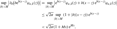 \begin{align*}\sup_{|b|< M}\bigl|\partial_{b}\bigl(b{\mathrm{e}}^{b(x-z)}\varphi_{\alpha,k}(z)\bigr)\bigr|&=\sup_{|b|< M}\bigl|{\mathrm{e}}^{b(x-z)}\varphi_{\alpha,k}(z)+b(x-z)\,{\mathrm{e}}^{b(x-z)}\varphi_{\alpha,k}(z)\bigr|\\[5pt] &\le\sqrt{2\alpha}\sup_{|b|< M}(1+|b|(x-z))\,{\mathrm{e}}^{b(x-z)} \\[5pt] &<\sqrt{2\alpha}(1+Mx)\,{\mathrm{e}}^{Mx},\end{align*}
which is integrable on (0, x] with respect to $\mathrm{d} z$
. Hence the Lebesgue convergence theorem yields that
$\mathrm{d} z$
. Hence the Lebesgue convergence theorem yields that $b\mapsto\Psi_{\alpha,k}(x;\;b)$
is of
$b\mapsto\Psi_{\alpha,k}(x;\;b)$
is of $C^1(\mathbb{R})$
.
$C^1(\mathbb{R})$
.
Lemma C.6. Under the assumptions S1, S2, and M[2], the following hold true:
-
(a)
$\displaystyle \sup_{x\in \mathbb{R}_+}|P(x;\;\widehat{p}_{n},0,\widehat{D}_{n})-P(x;\;p_0,0,D_0)|\stackrel{p}{\to} 0$
, -
(b)
$\displaystyle \sup_{x\in \mathbb{R}_+}|Q_{\alpha,k}(x;\;\widehat{p}_{n},0,\widehat{D}_{n})-Q_{\alpha,k}(x;\;p_0,0,D_0)|\stackrel{p}{\to} 0$
, -
(c)
$\displaystyle \sup_{x\in \mathbb{R}_+}|P^*(x;\;\widehat{p}_{n},0,\widehat{D}_{n})-P^*(x;\;p_0,0,D_0)|\stackrel{p}{\to} 0$
, -
(d)
$\displaystyle \sup_{x\in \mathbb{R}_+}|Q^*_{\alpha,k}(x;\;\widehat{p}_{n},0,\widehat{D}_{n})-Q^*_{\alpha,k}(x;\;p_0,0,D_0)|\stackrel{p}{\to} 0$
.


Proof. As for (a) with $D>0$
, it follows from the mean value theorem that
$D>0$
, it follows from the mean value theorem that
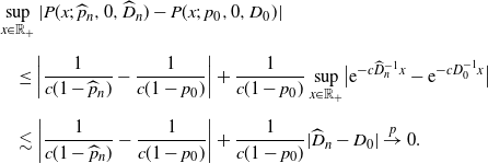 \begin{align*}&\sup_{x\in\mathbb{R}_+}|P(x;\;\widehat{p}_{n},0,\widehat{D}_{n})-P(x;\;p_0,0,D_0)| \\[5pt] &\quad \le \biggl|\dfrac{1}{c(1-\widehat{p}_{n})}-\dfrac{1}{c(1-p_0)}\biggr|+\dfrac{1}{c(1-p_0)}\sup_{x\in\mathbb{R}_+}\bigl|{\mathrm{e}}^{-c\widehat{D}_{n}^{-1}x}-{\mathrm{e}}^{-cD_0^{-1}x}\bigr| \\[5pt] &\quad \lesssim \biggl|\dfrac{1}{c(1-\widehat{p}_{n})}-\dfrac{1}{c(1-p_0)}\biggr|+\dfrac{1}{c(1-p_0)}|\widehat{D}_{n}-D_0| \stackrel{p}{\to} 0.\end{align*}
The proofs for (b)–(d) are similar by using the fact (2.2). The case of $D=0$
is also similar.
$D=0$
is also similar.
C.4. Proof of Lemma 2.1
Note the explicit expression in Feng and Shimizu [Reference Feng and Shimizu9, Proposition 4.1]:
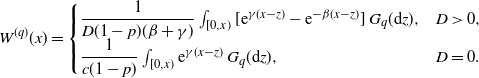 \begin{align*}W^{(q)}(x) = \begin{cases}\dfrac{1}{D(1-p)(\beta+ \gamma)}\int_{[0,x)} [{\mathrm{e}}^{\gamma(x-z)} - {\mathrm{e}}^{-\beta(x-z)}]\,G_q(\mathrm{d} z), & D>0, \\[5pt] \dfrac{1}{c(1-p)}\int_{[0,x)} {\mathrm{e}}^{\gamma(x-z)}\,G_q(\mathrm{d} z),& D=0.\end{cases}\end{align*}
By the integration by parts of this expression by noticing the jump at the origin, we have the result.
C.5. Proof of Lemma 2.5
We will show only the case where $D>0$
. The same calculation applies for
$D>0$
. The same calculation applies for $D=0$
. According to Lemmas 2.2 and 2.3, we should show that
$D=0$
. According to Lemmas 2.2 and 2.3, we should show that $f\;:\!=\; \overline{G}_q$
satisfies (2.3).
$f\;:\!=\; \overline{G}_q$
satisfies (2.3).
Let ${\epsilon},M>0$
be any constants with
${\epsilon},M>0$
be any constants with ${\epsilon} < M$
. We firstly show that the infinite sum
${\epsilon} < M$
. We firstly show that the infinite sum
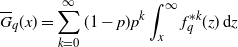 \begin{align*}\overline{G}_q(x)= \sum_{k=0}^\infty (1-p)p^k \int_x^\infty f_q^{*k}(z)\,\mathrm{d} z\end{align*}
can be differentiable under the summation sign on $({\epsilon},M)$
.
$({\epsilon},M)$
.
We shall put the partial sum
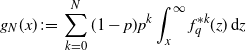 \begin{align*}g_N(x)\;:\!=\; \sum_{k=0}^N (1-p)p^k \int_x^\infty f_q^{*k}(z)\,\mathrm{d} z\end{align*}
for an integer $N \in \mathbb{N}$
, and note that
$N \in \mathbb{N}$
, and note that $g_N(x)\to \overline{G}_q(x)\ (N\to \infty)$
for all
$g_N(x)\to \overline{G}_q(x)\ (N\to \infty)$
for all $x>0$
. Next, note the differential formula for the convolution: for functions
$x>0$
. Next, note the differential formula for the convolution: for functions $f,g \in C^1(\mathbb{R}_+)$
,
$f,g \in C^1(\mathbb{R}_+)$
,
 \begin{align*}\dfrac{\mathrm{d} }{\mathrm{d} x} (f*g)(x) = (f * \partial_x g)(x) + f(x) g(0).\end{align*}
In particular, if $f(0)=0$
, then it follows for
$f(0)=0$
, then it follows for $k\in \mathbb{N}$
that
$k\in \mathbb{N}$
that
 \begin{align*}\partial_x f^{*k}= f*\partial_x f^{*(k-1)} = \cdots = f^{*(k-1)}*\partial_x f, \end{align*}
by induction. Using this formula, we have for $m=1,2,\ldots$
that
$m=1,2,\ldots$
that
 \begin{align*} \partial^m_x g_N(x) =p(1-p^{m-2})\partial_x^{m-1}f_q(x) - p^{m-1}\sum_{k=0}^{N-m+1} (1-p)p^k f_q^{*k}* \partial^{m-1}_xf_q(x),\end{align*}
where we regard $\partial_x^0 f_q \equiv 0$
as a convention. Now,
$\partial_x^0 f_q \equiv 0$
as a convention. Now, $f_q(x)$
is bounded by Lemma C.1, so
$f_q(x)$
is bounded by Lemma C.1, so $f_q^{*k}\ (k=1,2,\ldots)$
is also bounded. Moreover, it also follows that
$f_q^{*k}\ (k=1,2,\ldots)$
is also bounded. Moreover, it also follows that $\partial^m_xf_q$
is bounded on
$\partial^m_xf_q$
is bounded on $({\epsilon},M)$
. Indeed,
$({\epsilon},M)$
. Indeed,
 \begin{align*}\partial_x f_q(x) &= \dfrac{1}{pD}\biggl[-\beta f_q(x) + \overline{\nu}(x) + \int_x^\infty \overline{\nu}(z)\,\mathrm{d} z\biggr],\end{align*}
and we see by induction that for any $m\ge 2$
,
$m\ge 2$
,
 \begin{align*}|\partial_x^{m-1} f_q(x)| \lesssim 1+ \sum_{k=1}^{m-1} |\partial_x^{k-1} \overline{\nu}(x)| + \biggl|\int_x^\infty \overline{\nu}(z)\,\mathrm{d} z\biggr|.\end{align*}
Then it follows for any ${\epsilon}>0$
that
${\epsilon}>0$
that
 \begin{align}\sup_{x \in ({\epsilon},M)}|\partial_x^{m-1} f_q(x)| &\lesssim 1 + \sum_{k=1}^{m-1} \sup_{x \in ({\epsilon},M)} |\partial_x^{k-1} \overline{\nu}(x)| + \int_M^\infty \overline{\nu}(z)\,\mathrm{d} z\lesssim 1 + M^C, \end{align}
by the assumption (2.6). Therefore we can confirm the sequence $\{\partial^m_x g_N(x)\}_{N\in \mathbb{N}}$
is a uniform Cauchy sequence on
$\{\partial^m_x g_N(x)\}_{N\in \mathbb{N}}$
is a uniform Cauchy sequence on $({\epsilon},\infty)$
:
$({\epsilon},\infty)$
:
 \begin{align*}\lim_{N,N'\to \infty} \sup_{x\in ({\epsilon},M)}|\partial^m_x g_N(x) - \partial^m_x g_{N'}(x)| = 0.\end{align*}
Hence the term ‘differential theorem’ says that for any ${\epsilon}, M>0$
,
${\epsilon}, M>0$
,
 \begin{align*}\lim_{N\to \infty} \partial^m_x g_N(x)= \partial_x^m \overline{G}_q(x),\quad x \in ({\epsilon}, M).\end{align*}
Therefore it follows for any $x >0$
that
$x >0$
that
 \begin{align}\partial_x^m \overline{G}_q (x) &= p(1-p^{m-2})\partial_x^{m-1}f_q(x) - p^{m-1} \Biggl(\sum_{k=0}^\infty (1-p)p^k f_q^{*k} \Biggr)*\partial_x^{m-1}f_q \notag\\[5pt] &=p(1-p^{m-2})\partial_x^{m-1}f_q(x) -p^{m-1}\,\mathbb{E}\bigl[\partial_x^{m-1}f_q(x - Z)\bigr], \end{align}
where Z is a random variable with the distribution $G_q$
whose probability density is given by
$G_q$
whose probability density is given by $\sum_{k=0}^\infty (1-p)p^k f_q^{*k}(x)$
.
$\sum_{k=0}^\infty (1-p)p^k f_q^{*k}(x)$
.
Now, as for the second term in the last right-hand side of (C.3), we see that
 \begin{align*}\mathbb{E}\bigl[\partial_x^{m-1}f_q(x - Z)\bigr] = {\mathrm{O}}(1 + x^\kappa),\quad x\to \infty.\end{align*}
Indeed, it follows from (C.2) that
 \begin{align*}\sup_{x > {\epsilon}} \dfrac{|\partial_x^{m-1}f_q(x - Z)|}{1 + x^C} \lesssim \sup_{x > {\epsilon}} \dfrac{1 + x^C + Z^C}{1 + x^C} \le 1 + |Z|^C,\end{align*}
and the last term is integrable by the assumption. Then the Lebesgue convergence theorem and the equality (C.3) yield
 \begin{align*}\partial_x^m \overline{G}_q (x) & = {\mathrm{O}}(1 + x^\kappa),\quad x\to \infty,\end{align*}
which implies that $x^{m/2}\partial_x^m \overline{G}_q (x) \in L^2_\alpha(\mathbb{R}_+)$
for any
$x^{m/2}\partial_x^m \overline{G}_q (x) \in L^2_\alpha(\mathbb{R}_+)$
for any $\alpha>0$
and
$\alpha>0$
and $m\ge 2$
. Similarly, as in (2.8), we have
$m\ge 2$
. Similarly, as in (2.8), we have
 \begin{align*}|x^{m/2} \partial_x^m \overline{G}_q (x)|^2 {\mathrm{e}}^{-\alpha x}= {\mathrm{O}}(x^m {\mathrm{e}}^{-(\alpha -2k) x}),\quad x\to \infty,\end{align*}
and therefore $x^{m/2}\partial_x^m \overline{G}_q (x) \in L^2_\alpha(\mathbb{R}_+)$
for any
$x^{m/2}\partial_x^m \overline{G}_q (x) \in L^2_\alpha(\mathbb{R}_+)$
for any $\alpha>2\kappa$
. This completes the proof.
$\alpha>2\kappa$
. This completes the proof.
C.6. Proof of Theorem 3.1
As for the consistency, thanks to Corollary B.1 and Lemma C.5, the continuous mapping theorem yields that
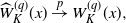 \begin{align*}\widehat{W}^{(q)}_{K}(x)\stackrel{p}{\to} W^{(q)}_{K}(x),\end{align*}
for each $x\in\mathbb{R}_+$
and
$x\in\mathbb{R}_+$
and $q\ge 0$
. In particular, as
$q\ge 0$
. In particular, as $q=0$
, noticing that
$q=0$
, noticing that $\widehat{\gamma}_{n}=\gamma_0=0$
, we see from Lemma C.6 that
$\widehat{\gamma}_{n}=\gamma_0=0$
, we see from Lemma C.6 that
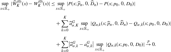 \begin{align*}\sup_{x\in\mathbb{R}_+}|\widehat{W}^{(0)}_{K}(x)-W^{(0)}_{K}(x)|&\leq\sup_{x\in\mathbb{R}_+}|P(x;\;\widehat{p}_{n},0,\widehat{D}_{n})-P(x;\;p_0,0,D_0)| \\[5pt] &\quad +\sum_{k=0}^{K}\widehat{a}^{G}_{\alpha,K}\sup_{x\in\mathbb{R}_+}|Q_{\alpha,k}(x;\;\widehat{p}_{n},0,\widehat{D}_{n})-Q_{\alpha,k}(x;\;p_0,0,D_0)|\\[5pt] &\quad +\sum_{k=0}^{K}\bigl|\widehat{a}^{G}_{\alpha,k}-a^{G}_{\alpha,k}\bigr|\sup_{x\in\mathbb{R}_+}|Q_{\alpha,k}(x;\;p_0,0,D_0)|\stackrel{p}{\to} 0.\end{align*}
As for the asymptotic normality, we only show the case where $D>0$
since the proof for
$D>0$
since the proof for $D=0$
is done similarly.
$D=0$
is done similarly.
Note that
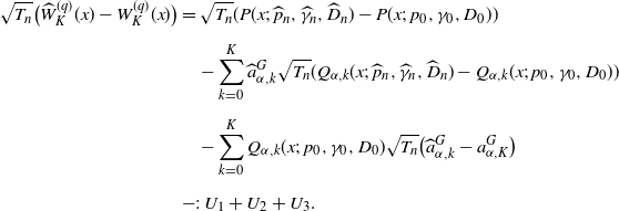 \begin{align*}\sqrt{T_{n}}\bigl(\widehat{W}^{(q)}_{K}(x)-W^{(q)}_{K}(x)\bigr)&=\sqrt{T_{n}}(P(x;\;\widehat{p}_{n},\widehat{\gamma}_{n},\widehat{D}_{n})-P(x;\;p_0,\gamma_0,D_0)) \\[5pt] &\quad -\sum_{k=0}^{K}\widehat{a}^{G}_{\alpha,k}\sqrt{T_{n}}(Q_{\alpha,k}(x;\;\widehat{p}_{n},\widehat{\gamma}_{n},\widehat{D}_{n})-Q_{\alpha,k}(x;\;p_0,\gamma_0,D_0))\\[5pt] &\quad -\sum_{k=0}^{K}Q_{\alpha,k}(x;\;p_0,\gamma_0,D_0)\sqrt{T_{n}}\bigl(\widehat{a}^{G}_{\alpha,k}-a^{G}_{\alpha,K}\bigr)\\[5pt] &=: U_1+U_2+U_3.\end{align*}
On $U_1$
, applying the mean value theorem, there exists some
$U_1$
, applying the mean value theorem, there exists some $p^{*}_{n}$
,
$p^{*}_{n}$
, $\gamma^{*}_{n}$
,
$\gamma^{*}_{n}$
, $D^{*}_{n}$
such that
$D^{*}_{n}$
such that
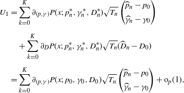 \begin{align*}U_1&=\sum_{k=0}^{K}\partial_{(p,\gamma)}P(x;\;p^{*}_{n},\gamma^{*}_{n},D^{*}_{n}) \sqrt{T_{n}} \begin{pmatrix} \widehat{p}_{n}-p_0\\[5pt] \widehat{\gamma}_{n}-\gamma_0 \end{pmatrix} \\[5pt] &\quad +\sum_{k=0}^{K}\partial_{D}P(x;\;p^{*}_{n},\gamma^{*}_{n},D^{*}_{n})\sqrt{T_{n}}(\widehat{D}_{n}-D_0)\\[5pt] &= \sum_{k=0}^{K}\partial_{(p,\gamma)}P(x;\;p_0,\gamma_0,D_0) \sqrt{T_{n}} \begin{pmatrix} \widehat{p}_{n}-p_0\\[5pt] \widehat{\gamma}_{n}-\gamma_0 \end{pmatrix}+ {\mathrm{o}}_p(1),\end{align*}
by Lemma A.1 and the continuous mapping theorem. By an argument similar to that above, we have
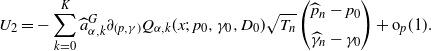 \begin{align*}U_{2}=-\sum_{k=0}^{K}\widehat{a}^{G}_{\alpha,k}\partial_{(p,\gamma)}Q_{\alpha,k}(x;\;p_0,\gamma_0,D_0)\sqrt{T_{n}} \begin{pmatrix} \widehat{p}_{n}-p_0\\[5pt] \widehat{\gamma}_{n}-\gamma_0 \end{pmatrix} +{\mathrm{o}}_{p}(1).\end{align*}
Moreover, on $U_3$
, we obtain by (B.4) in Corollary B.1 that
$U_3$
, we obtain by (B.4) in Corollary B.1 that
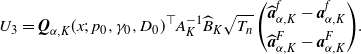 \begin{align*}U_3={\boldsymbol{Q}}_{\alpha,K}(x;\;p_0,\gamma_0,D_0)^\top A_{K}^{-1}\widehat{B}_{K}\sqrt{T_{n}} \begin{pmatrix} \widehat{\boldsymbol{a}}^{f}_{\alpha,K}-\boldsymbol{a}^{f}_{\alpha,K}\\[5pt] \widehat{\boldsymbol{a}}^{F}_{\alpha,K}-\boldsymbol{a}^{F}_{\alpha,K} \end{pmatrix}\!.\end{align*}
As a consequence, we have
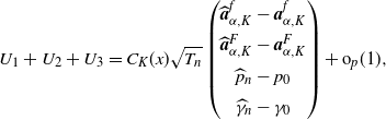 \begin{align}U_1+U_2+U_3=C_K(x)\sqrt{T_{n}} \begin{pmatrix} \widehat{\boldsymbol{a}}^{f}_{\alpha,K}-\boldsymbol{a}^{f}_{\alpha,K}\\[5pt] \widehat{\boldsymbol{a}}^{F}_{\alpha,K}-\boldsymbol{a}^{F}_{\alpha,K}\\[5pt] \widehat{p}_{n}-p_0\\[5pt] \widehat{\gamma}_{n}-\gamma_0 \end{pmatrix}+{\mathrm{o}}_{p}(1), \end{align}
and Theorem B.2 yields the result.
C.7. Proof of Theorem 3.2
By the same argument as in the proof of Theorem 3.1 in Section C.6, we have
 \begin{align}\sqrt{T_{n}}\bigl(\widehat{Z}^{(q)}_{K}(x)-Z^{(q)}_{K}(x)\bigr)= qC^*_K(x)\sqrt{T_{n}} \begin{pmatrix} \widehat{\boldsymbol{a}}^{f}_{\alpha,K}-\boldsymbol{a}^{f}_{\alpha,K}\\[5pt] \widehat{\boldsymbol{a}}^{F}_{\alpha,K}-\boldsymbol{a}^{F}_{\alpha,K}\\[5pt] \widehat{p}_{n}-p_0\\[5pt] \widehat{\gamma}_{n}-\gamma_0 \end{pmatrix}+{\mathrm{o}}_{p}(1), \end{align}
and Theorem B.2 yields the result.
C.8. Proof of Theorem 3.1
Noticing the expressions (C.4) and (C.5), we have
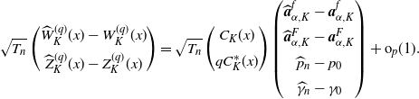 \begin{align*}\sqrt{T_{n}} \begin{pmatrix} \widehat{W}^{(q)}_{K}(x)-W^{(q)}_{K}(x)\\[5pt] \widehat{Z}^{(q)}_{K}(x)-Z^{(q)}_{K}(x) \end{pmatrix} = \sqrt{T_n} \begin{pmatrix} C_{K}(x)\\[5pt] qC^{*}_{K}(x) \end{pmatrix} \begin{pmatrix} \widehat{\boldsymbol{a}}^{f}_{\alpha,K}-\boldsymbol{a}^{f}_{\alpha,K}\\[5pt] \widehat{\boldsymbol{a}}^{F}_{\alpha,K}-\boldsymbol{a}^{F}_{\alpha,K}\\[5pt] \widehat{p}_{n}-p_0\\[5pt] \widehat{\gamma}_{n}-\gamma_0 \end{pmatrix} + {\mathrm{o}}_p(1).\end{align*}
Then Theorem B.2 yields the result.
Acknowledgements
The authors sincerely thank the anonymous reviewers for their insightful comments, which have enhanced the quality of this paper.
Funding information
This work is partially supported by JSPS KAKENHI Grant-in-Aid for Scientific Research (C) #21K03358 Japan Science and Technology Agency CREST #JPMJCR2115.
Competing interests
There were no competing interests to declare which arose during the preparation or publication process of this article.

 Open access