


1 Introduction
1.1 Motivation and Results
Since Bridgeland [Reference BridgelandBri07] defined the notion of stability conditions on derived categories, its construction on a given threefold has been an important open problem. It turned out that, to solve this problem, we need a Bogomolov–Gieseker (BG) type inequality, involving the third Chern character, for certain stable objects in the derived category [Reference Bayer, Macrì and StellariBMS16, Reference Bayer, Macrì and TodaBMT14, Reference Bernardara, Macrì, Schmidt and ZhaoBMSZ17]. There are several classes of threefolds on which we know the existence of Bridgeland stability conditions [Reference Bayer, Macrì and StellariBMS16, Reference Bayer, Macrì and TodaBMT14, Reference Bernardara, Macrì, Schmidt and ZhaoBMSZ17, Reference KosekiKos17, Reference KosekiKos20, Reference LiLi19a, Reference LiLi19b, Reference LiuLiu21a, Reference LiuLiu21b, Reference Maciocia and PiyaratneMP16a, Reference Maciocia and PiyaratneMP16b, Reference MacrìMacr14, Reference PiyaratnePiy17, Reference SchmidtSch14]. For K-trivial threefolds, the only known cases are the quintic threefolds [Reference LiLi19a], abelian threefolds and their étale quotients [Reference Bayer, Macrì and StellariBMS16, Reference Maciocia and PiyaratneMP16a, Reference Maciocia and PiyaratneMP16b].
Among them, Li [Reference LiLi19a] recently treated quintic threefolds, which is one of the most important cases for mirror symmetry. The crucial step in his arguments is to establish the improvement of the classical BG inequality for torsion free slope stable sheaves. Recall that a version of the classical BG inequality is the inequality
 $$ \begin{align} \frac{H\operatorname{\mathrm{ch}}_2(E)}{H^3\operatorname{\mathrm{ch}}_0(E)} \leq \frac{1}{2}\left( \frac{H^2\operatorname{\mathrm{ch}}_1(E)}{H^3\operatorname{\mathrm{ch}}_0(E)} \right)^2,\\[-15pt]\nonumber \end{align} $$
where E is a slope stable sheaf with respect to an ample divisor H. For del Pezzo and K3 surfaces, we can easily get the inequality stronger than equation (1), simply by using the Serre duality. In contrast, such an improvement of the BG inequality on Calabi–Yau threefolds is highly nontrivial.
When the first draft of this paper was submitted, the arguments in [Reference LiLi19a] have been applied only for quintic threefolds. Very recently, Liu [Reference LiuLiu21a] treated Calabi–Yau complete intersections of quadratic and quartic hypersurfaces in $\mathbb {P}^5$
via a similar method. The goal of the present paper is to extend it to two other examples of Calabi–Yau threefolds, namely, general weighted hypersurfaces in the weighted projective spaces
$\mathbb {P}^5$
via a similar method. The goal of the present paper is to extend it to two other examples of Calabi–Yau threefolds, namely, general weighted hypersurfaces in the weighted projective spaces $\mathbb {P}(1, 1, 1, 1, 2)$
and
$\mathbb {P}(1, 1, 1, 1, 2)$
and $\mathbb {P}(1, 1, 1, 1, 4)$
. We call them as triple/double cover CY3 since they have finite morphisms to
$\mathbb {P}(1, 1, 1, 1, 4)$
. We call them as triple/double cover CY3 since they have finite morphisms to $\mathbb {P}^3$
of degree
$\mathbb {P}^3$
of degree $3$
,
$3$
, $2$
, respectively. The following is our main result:
$2$
, respectively. The following is our main result:
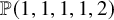
Theorem 1.1 (Theorems 4.1, 5.4)
Let X be a double or triple cover CY3, H the primitive ample divisor and E a slope stable sheaf with slope $\mu \in [-1, 1]$
. Then the inequality
$\mu \in [-1, 1]$
. Then the inequality
 $$ \begin{align} \frac{H\operatorname{\mathrm{ch}}_2(E)}{H^3\operatorname{\mathrm{ch}}_0(E)} \leq \Xi\left(\left| \frac{H^2\operatorname{\mathrm{ch}}_1(E)}{H^3\operatorname{\mathrm{ch}}_0(E)} \right|\right)\\[-15pt]\nonumber \end{align} $$
holds. Here, the function $\Xi $
is defined as follows.
$\Xi $
is defined as follows.
 $$\begin{align*}\Xi(t):=\left\{ \begin{array}{ll} t^2-t & (t \in [0, 1/4]) \\ 3t/4-3/8 & (t \in [1/4, 1/2]) \\ t/4-1/8 & (t \in [1/2, 3/4]) \\ t^2-1/2 & (t \in [3/4, 1]). \end{array} \right.\\[-25pt] \end{align*}$$
See Figure 1 for the graph of the function $\Xi$
. Using this stronger BG inequality, we prove the following BG type inequality (involving
$\Xi$
. Using this stronger BG inequality, we prove the following BG type inequality (involving $\operatorname {\mathrm {ch}}_3$
) for
$\operatorname {\mathrm {ch}}_3$
) for $\nu _{\beta , \alpha }$
-stable objects, which are certain two term complexes in the derived category. For the precise definition of
$\nu _{\beta , \alpha }$
-stable objects, which are certain two term complexes in the derived category. For the precise definition of $\nu _{\beta , \alpha }$
-stability, see Section 2.
$\nu _{\beta , \alpha }$
-stability, see Section 2.
Theorem 1.2 (Theorem 2.3, Corollary 6.4)
Let X be a double or triple cover CY3, take real numbers $\alpha , \beta \in \mathbb {R}$
with
$\alpha , \beta \in \mathbb {R}$
with $\alpha> \frac {1}{2}\beta ^2 +\frac {1}{2}(\beta -\lfloor \beta \rfloor ) (\lfloor \beta \rfloor +1-\beta )$
. Let E be a
$\alpha> \frac {1}{2}\beta ^2 +\frac {1}{2}(\beta -\lfloor \beta \rfloor ) (\lfloor \beta \rfloor +1-\beta )$
. Let E be a $\nu _{\beta , \alpha }$
-semistable object. Then the inequality
$\nu _{\beta , \alpha }$
-semistable object. Then the inequality
 $$\begin{align*}Q^\Gamma_{\alpha, \beta}(E) \geq 0\\[-15pt] \end{align*}$$
holds. Here, we put $\Gamma :=\frac {2}{9}H^2$
(resp.
$\Gamma :=\frac {2}{9}H^2$
(resp. $\frac {1}{3}H^2$
) when X is a triple (resp. double) cover CY3, and the quadratic form
$\frac {1}{3}H^2$
) when X is a triple (resp. double) cover CY3, and the quadratic form $Q^\Gamma _{\alpha , \beta }$
is defined as follows:
$Q^\Gamma _{\alpha , \beta }$
is defined as follows:
 $$ \begin{align*} Q^\Gamma_{\alpha, \beta}(E)&:= (2\alpha-\beta^2)\left( \overline{\Delta}_{H}(E)+3\frac{\Gamma.H}{H^3} \left(H^3\operatorname{\mathrm{ch}}^\beta_0(E) \right)^2 \right) \\ &\quad +2\left(H\operatorname{\mathrm{ch}}^\beta_2(E) \right)\left( 2H\operatorname{\mathrm{ch}}^\beta_2(E)-3\Gamma.H \operatorname{\mathrm{ch}}^\beta_0(E) \right) \\ &\quad -6\left(H^2\operatorname{\mathrm{ch}}^\beta_1(E) \right) \left( \operatorname{\mathrm{ch}}^\beta_3(E)-\Gamma\operatorname{\mathrm{ch}}_1^\beta(E) \right). \end{align*} $$

Figure 1 Strong BG inequality on double/triple cover CY3s.
The above theorem enables us to construct an open subset in the space of Bridgeland stability conditions [Reference Bayer, Macrì and StellariBMS16, Reference Bayer, Macrì and TodaBMT14, Reference Bernardara, Macrì, Schmidt and ZhaoBMSZ17]. For real numbers $\alpha , \beta , a, b$
, we define a group homomorphism
$\alpha , \beta , a, b$
, we define a group homomorphism $Z^{a, b}_{\beta , \alpha } \colon K(X) \to \mathbb {C}$
as
$Z^{a, b}_{\beta , \alpha } \colon K(X) \to \mathbb {C}$
as
 $$\begin{align*}Z^{a, b}_{\beta, \alpha}:= -\operatorname{\mathrm{ch}}_3^{\beta}+bH\operatorname{\mathrm{ch}}_2^\beta+aH^2\operatorname{\mathrm{ch}}_1^\beta +i\left( H\operatorname{\mathrm{ch}}_2^\beta-\frac{1}{2}\alpha^2H^3\operatorname{\mathrm{ch}}_0^\beta \right). \end{align*}$$
We denote by $\mathcal {A}^{\beta , \alpha }$
the double-tilted heart defined in [Reference Bayer, Macrì and TodaBMT14].
$\mathcal {A}^{\beta , \alpha }$
the double-tilted heart defined in [Reference Bayer, Macrì and TodaBMT14].
Theorem 1.3 (Theorem 7.2)
We have a continuous family $\left (Z^{a, b}_{\beta , \alpha }, \mathcal {A}^{\beta , \alpha } \right )$
of stability conditions parametrized by real numbers
$\left (Z^{a, b}_{\beta , \alpha }, \mathcal {A}^{\beta , \alpha } \right )$
of stability conditions parametrized by real numbers $\alpha , \beta , a, b$
satisfying
$\alpha , \beta , a, b$
satisfying
 $$\begin{align*}\alpha> 0, \quad \alpha^2+\left(\beta-\lfloor\beta \rfloor-\frac{1}{2} \right)^2 > \frac{1}{4}, \quad a > \frac{1}{6}\alpha^2+\frac{1}{2}|b|\alpha+\gamma, \end{align*}$$
where we put $\gamma :=2/9$
(resp.
$\gamma :=2/9$
(resp. $1/3$
) when X is a triple (resp. double) cover CY3. Acting by the group
$1/3$
) when X is a triple (resp. double) cover CY3. Acting by the group $\widetilde {\operatorname {\mathrm {GL}}^+}(2; \mathbb {R})$
, it forms an open subset in the space of stability conditions.
$\widetilde {\operatorname {\mathrm {GL}}^+}(2; \mathbb {R})$
, it forms an open subset in the space of stability conditions.
1.2 Strategy of the proof
In this subsection, we briefly explain how to prove Theorem 1.1. Let us first recall the arguments in [Reference LiLi19a] for a quintic threefold $X_5 \subset \mathbb {P}^4$
. We consider
$X_5 \subset \mathbb {P}^4$
. We consider $(2, 2, 5)$
,
$(2, 2, 5)$
, $(2, 5)$
,
$(2, 5)$
, $(2, 2)$
complete intersections
$(2, 2)$
complete intersections
 $$\begin{align*}C_{2, 2, 5} \subset T_{2, 5} \subset X_5, \quad C_{2, 2, 5} \subset S_{2, 2}. \end{align*}$$
The stronger BG inequality on $X_5$
is proved in the following way:
$X_5$
is proved in the following way:
-
1. First, we reduce the problem to proving the same inequality for stable sheaves on the surface $T_{2, 5} \subset X_5$
by using the restriction technique.
$T_{2, 5} \subset X_5$
by using the restriction technique. -
2. Again using the restriction, the problem is further reduced to establishing a stronger Clifford type bounds on global sections for stable vector bundles on the curve
$C_{2, 2, 5} \subset T_{2, 5}$
. -
3. Regard the stable vector bundle on
$C_{2, 2, 5}$
as a torsion sheaf on the surface
$S_{2, 2}$
via the inclusion
$C_{2, 2, 5} \subset S_{2, 2}$
. Then a wall-crossing argument in the space of Bridgeland stability conditions on the surface
$S_{2, 2}$
gives the desired Clifford type bounds. The argument in this step first appeared in [Reference FeyzbakhshFey20].


In step (3), the crucial fact is that the surface $S_{2, 2}$
is del Pezzo, on which a stronger BG inequality holds.
$S_{2, 2}$
is del Pezzo, on which a stronger BG inequality holds.
For double/triple cover CY3s, the situation is quite similar. In fact, we have smooth complete intersection varieties
 $$ \begin{align*} &C_{2, 2, 6} \subset T_{2, 6} \subset X_6, \quad C_{2, 2, 6} \subset S_{2, 2} \quad \mbox{ in } \mathbb{P}(1, 1, 1, 1, 2), \\ &C_{2, 4, 8} \subset T_{2, 8} \subset X_8, \quad C_{2, 4, 8} \subset S_{2, 4} \quad \mbox{ in } \mathbb{P}(1, 1, 1, 1, 4), \end{align*} $$
where both of the surfaces $S_{2, 2} \subset \mathbb {P}(1, 1, 1, 1, 2)$
and
$S_{2, 2} \subset \mathbb {P}(1, 1, 1, 1, 2)$
and $S_{2, 4} \subset \mathbb {P}(1, 1, 1, 1, 4)$
are isomorphic to the quadric surface
$S_{2, 4} \subset \mathbb {P}(1, 1, 1, 1, 4)$
are isomorphic to the quadric surface $\mathbb {P}^1 \times \mathbb {P}^1$
, which is del Pezzo. Note that we consider
$\mathbb {P}^1 \times \mathbb {P}^1$
, which is del Pezzo. Note that we consider $(2, 4)$
complete intersection in
$(2, 4)$
complete intersection in $\mathbb {P}(1, 1, 1, 1, 4)$
instead of
$\mathbb {P}(1, 1, 1, 1, 4)$
instead of $(2, 2)$
, to avoid the singularity.
$(2, 2)$
, to avoid the singularity.
Hence, we are able to apply the methods in [Reference LiLi19a] to our cases. At this moment, we do not know the way to treat these examples uniformly, so the author believes it is still worth writing down the complete proofs. In fact, it turns out that, in our cases, we need the modified term $\Gamma $
in Theorem 1.2, unlike the quintic case.
$\Gamma $
in Theorem 1.2, unlike the quintic case.
1.3 Open problems
-
1. In Theorem 1.2, we expect we can take
$\Gamma =0$
. For this, we need a further improvement of Theorem 1.1. -
2. Stability conditions we construct in this paper are said to be ‘near the large volume limit’ in physics. For weighted hypersurfaces, we expect the existence of another kind of stability conditions, called Gepner type. Mathematically, it is the stability condition invariant under the certain autoequivalence of the derived category. See [Reference TodaTod14, Reference TodaTod17] for discussions on the construction of Gepner type stability conditions. To construct the heart corresponding to the Gepner type stability condition, the first task is to prove a stronger form of the BG inequality for stable sheaves with a specific slope equal
$-1/2$
. Unfortunately, Theorem 1.1 is not enough for this purpose. -
3. One might ask whether we can treat other Calabi–Yau weighted hypersurfaces inside
$\mathbb {P}(a_1, a_2, a_3, a_4, a_5)$
with more general weights
$(a_i)$
. Unfortunately, quintic and double/triple cover CY3s are the only cases where
$\mathbb {P}(a_1, a_2, a_3, a_4, a_5)$
contains a smooth Calabi–Yau hypersurface and a smooth del Pezzo (or K3) complete intersection surface at the same time. Indeed, it happens precisely when the weighted
$\mathbb {P}^4$
has only isolated singularities and its canonical line bundle can be written as
$L^{\otimes m}$
, where L is a free line bundle and
$m \geq 2$
. These conditions are equivalent to the following numerical conditions.-
○ For any i with
$a_i>1$
and for any
$j \neq i$
,
$a_i$
does not divide
$a_j$
, -
○
$\sum a_i=m \cdot \operatorname {\mathrm {lcm}}(a_i)$
.
An easy but lengthy calculation show that there are only three solutions. If we allow smooth Deligne–Mumford stacks, i.e., if we allow the weighted
$\mathbb {P}^4$
to have nonisolated singularities, there are several other solutions. -


1.4 Plan of the paper
The paper is organized as follows. In Section 2, we recall about the notion of tilt stability in the derived category and about the BG type inequality conjecture. Sections 3 and 4 are devoted to proving Theorem 1.1 for a triple cover CY3. The key ingredient is the stronger Clifford type bound proved in Section 3. In Section 5, we treat the case of a double cover CY3. In Section 6, we prove Theorem 1.2. Finally, in Section 7, we prove Theorem 1.3.
Notation and Convention. In this paper, we always work over the complex number field $\mathbb {C}$
. We will use the following notations.
$\mathbb {C}$
. We will use the following notations.
-
○ For an ample divisor H and a real number
$\beta \in \mathbb {R}$
, we denote by
$\operatorname {\mathrm {ch}}^\beta =(\operatorname {\mathrm {ch}}^\beta _0, \cdots , \operatorname {\mathrm {ch}}^\beta _n):=e^{-\beta H}\operatorname {\mathrm {ch}}$
, the
$\beta $
-twisted Chern character. -
○
$\hom (E, F):=\dim \operatorname {\mathrm {Hom}}(E, F)$
, and
$\operatorname {\mathrm {ext}}^i(E, F):=\dim \operatorname {\mathrm {Ext}}^i(E, F)$
for objects
$E, F$
in the derived category, and an integer i.


2 Preliminaries
2.1 BG type inequality conjecture
In this subsection, we recall the notion of tilt stability, and the BG type inequality conjecture. We mainly follow the notations in the paper [Reference LiLi19a]. Let X be a smooth projective variety of dimension $n \geq 2$
, H an ample divisor. We take real numbers
$n \geq 2$
, H an ample divisor. We take real numbers $\alpha , \beta \in \mathbb {R}$
with
$\alpha , \beta \in \mathbb {R}$
with $\alpha> \frac {1}{2} \beta ^2$
. We define a slope function
$\alpha> \frac {1}{2} \beta ^2$
. We define a slope function $\mu _H$
as follows:
$\mu _H$
as follows:
 $$\begin{align*}\mu_H:=\frac{H^{n-1}\operatorname{\mathrm{ch}}_1}{H^n\operatorname{\mathrm{ch}}_0} \colon \operatorname{\mathrm{Coh}}(X) \to \mathbb{R} \cup \{+\infty\}. \end{align*}$$
We have the notion of $\mu _H$
-stability on
$\mu _H$
-stability on $\operatorname {\mathrm {Coh}}(X)$
and the corresponding torsion pair on
$\operatorname {\mathrm {Coh}}(X)$
and the corresponding torsion pair on $\operatorname {\mathrm {Coh}}(X)$
:
$\operatorname {\mathrm {Coh}}(X)$
:
 $$ \begin{align*} &\mathcal{T}_\beta:=\left\langle T \in \operatorname{\mathrm{Coh}}(X) : T \mbox{ is } \mu_H \mbox{-semistable with } \mu_H(T)>\beta \right\rangle, \\ &\mathcal{F}_\beta:=\left\langle F \in \operatorname{\mathrm{Coh}}(X) : F \mbox{ is } \mu_H \mbox{-semistable with } \mu_H(F) \leq \beta \right\rangle. \end{align*} $$
Here, $\langle S \rangle $
denotes the extension closure of a set
$\langle S \rangle $
denotes the extension closure of a set $S \subset \operatorname {\mathrm {Coh}}(X)$
of objects in the category
$S \subset \operatorname {\mathrm {Coh}}(X)$
of objects in the category $\operatorname {\mathrm {Coh}}(X)$
. By the general theory of torsion pairs [Reference Happel, Reiten and SmaløHRS96], we obtain the new abelian category
$\operatorname {\mathrm {Coh}}(X)$
. By the general theory of torsion pairs [Reference Happel, Reiten and SmaløHRS96], we obtain the new abelian category
 $$\begin{align*}\operatorname{\mathrm{Coh}}^\beta(X):=\left\langle \mathcal{F}_\beta[1], \mathcal{T}_\beta \right\rangle \subset D^b(X), \end{align*}$$
which is the heart of a bounded t-structure on $D^b(X)$
. On the heart
$D^b(X)$
. On the heart $\operatorname {\mathrm {Coh}}^\beta (X)$
, we define the following slope function:
$\operatorname {\mathrm {Coh}}^\beta (X)$
, we define the following slope function:
 $$\begin{align*}\nu_{\beta, \alpha}:= \frac{H^{n-2}\operatorname{\mathrm{ch}}_2-\alpha H^n\operatorname{\mathrm{ch}}_0}{H^{n-1}\operatorname{\mathrm{ch}}_1-\beta H^n\operatorname{\mathrm{ch}}_0} \colon \operatorname{\mathrm{Coh}}^\beta(X) \to \mathbb{R} \cup \{+\infty\}. \end{align*}$$
Then as similar to the $\mu _H$
-stability on
$\mu _H$
-stability on $\operatorname {\mathrm {Coh}}(X)$
, we can define the notion of
$\operatorname {\mathrm {Coh}}(X)$
, we can define the notion of $\nu _{\beta , \alpha }$
-stability on
$\nu _{\beta , \alpha }$
-stability on $\operatorname {\mathrm {Coh}}^\beta (X)$
. We also call
$\operatorname {\mathrm {Coh}}^\beta (X)$
. We also call $\nu _{\alpha , \beta }$
-stability as tilt-stability.
$\nu _{\alpha , \beta }$
-stability as tilt-stability.
Definition 2.1. Let $E \in \operatorname {\mathrm {Coh}}^0(X)$
be an object.
$E \in \operatorname {\mathrm {Coh}}^0(X)$
be an object.
-
1. We define the Brill–Noether (BN) slope of E as
$$\begin{align*}\nu_{BN}(E):= \frac{H^{n-2}\operatorname{\mathrm{ch}}_2(E)}{H^{n-1}\operatorname{\mathrm{ch}}_1(E)} \in \mathbb{R} \cup \{+\infty\}. \end{align*}$$
-
2. We say the object E is Brill–Noether (BN) (semi)stable if it is
$\nu _{0, \alpha }$
-(semi)stable for every sufficiently small real number
$0 < \alpha \ll 1$
.


We refer [Reference LiLi19a, Section 2] for the basic properties of tilt stability and BN stability. Let us define the discriminant of an object $E \in D^b(X)$
as
$E \in D^b(X)$
as
 $$\begin{align*}\overline{\Delta}_H(E):= (H^{n-1}\operatorname{\mathrm{ch}}_1(E))^2-2H^n\operatorname{\mathrm{ch}}_0(E)H^{n-2}\operatorname{\mathrm{ch}}_2(E). \end{align*}$$
The following is the main question we investigate in this paper.
Question 2.2 [Reference Bayer, Macrì and StellariBMS16, Reference Bayer, Macrì and TodaBMT14, Reference Bernardara, Macrì, Schmidt and ZhaoBMSZ17]
Assume that $n=\dim X=3$
. Find a
$n=\dim X=3$
. Find a $1$
-cycle
$1$
-cycle $\Gamma \in A_1(X)_{\mathbb {R}}$
satisfying
$\Gamma \in A_1(X)_{\mathbb {R}}$
satisfying $\Gamma .H \geq 0$
, and the following property: Let E be a
$\Gamma .H \geq 0$
, and the following property: Let E be a $\nu _{\beta , \alpha }$
-semistable object. Then the inequality
$\nu _{\beta , \alpha }$
-semistable object. Then the inequality
 $$\begin{align*}Q^\Gamma_{\alpha, \beta}(E) \geq 0 \end{align*}$$
holds. Here, the quadratic form $Q^\Gamma _{\alpha , \beta }$
is defined as follows:
$Q^\Gamma _{\alpha , \beta }$
is defined as follows:
 $$ \begin{align*} Q^\Gamma_{\alpha, \beta}(E)&:= (2\alpha-\beta^2)\left( \overline{\Delta}_{H}(E)+3\frac{\Gamma.H}{H^3} \left(H^3\operatorname{\mathrm{ch}}^\beta_0(E) \right)^2 \right) \\ &\quad +2\left(H\operatorname{\mathrm{ch}}^\beta_2(E) \right)\left( 2H\operatorname{\mathrm{ch}}^\beta_2(E)-3\Gamma.H \operatorname{\mathrm{ch}}^\beta_0(E) \right) \\ &\quad -6\left(H^2\operatorname{\mathrm{ch}}^\beta_1(E) \right) \left( \operatorname{\mathrm{ch}}^\beta_3(E)-\Gamma\operatorname{\mathrm{ch}}_1^\beta(E) \right). \end{align*} $$
The conjectural inequality above is called the Bogomolov–Gieseker (BG) type inequality conjecture, proposed in [Reference Bayer, Macrì and StellariBMS16, Reference Bayer, Macrì and TodaBMT14] with $\Gamma =0$
. It is known that the BG type inequality conjecture with
$\Gamma =0$
. It is known that the BG type inequality conjecture with $\Gamma =0$
fails for some classes of threefolds, such as the blow-up of
$\Gamma =0$
fails for some classes of threefolds, such as the blow-up of $\mathbb {P}^3$
at a point (cf. [Reference KosekiKos17, Reference Martinez and SchmidtMS19, Reference SchmidtSch17]). The question with the modified term
$\mathbb {P}^3$
at a point (cf. [Reference KosekiKos17, Reference Martinez and SchmidtMS19, Reference SchmidtSch17]). The question with the modified term $\Gamma $
appeared in [Reference Bernardara, Macrì, Schmidt and ZhaoBMSZ17] and proved affirmatively for all Fano threefolds.
$\Gamma $
appeared in [Reference Bernardara, Macrì, Schmidt and ZhaoBMSZ17] and proved affirmatively for all Fano threefolds.
The following reduction of Question 2.2 plays an important role in this paper.
Theorem 2.3 (cf. [Reference LiLi19a, Theorem 3.2])
Assume that $n=\dim X=3$
. Let
$n=\dim X=3$
. Let $\Gamma $
be a
$\Gamma $
be a $1$
-cycle with
$1$
-cycle with $\Gamma .H \geq 0$
. Suppose that for every BN stable object with
$\Gamma .H \geq 0$
. Suppose that for every BN stable object with $\nu _{BN}(E) \in [0, 1/2]$
, the inequality
$\nu _{BN}(E) \in [0, 1/2]$
, the inequality $Q^\Gamma _{0, 0}(E) \geq 0$
holds.
$Q^\Gamma _{0, 0}(E) \geq 0$
holds.
Then the inequality in Question 2.2 holds for any choice of real numbers $\alpha , \beta \in \mathbb {R}$
with
$\alpha , \beta \in \mathbb {R}$
with $\alpha> \frac {1}{2}\beta ^2 +\frac {1}{2}(\beta -\lfloor \beta \rfloor ) (\lfloor \beta \rfloor +1-\beta )$
.
$\alpha> \frac {1}{2}\beta ^2 +\frac {1}{2}(\beta -\lfloor \beta \rfloor ) (\lfloor \beta \rfloor +1-\beta )$
.
Proof. Exactly the same arguments as in [Reference LiLi19a, Theorem 3.2] work since the following statements are true.
-
○ Let
$(\beta ', \alpha ') \in \mathbb {R}^2$
be a point on the line through
$p_H(E)$
and
$(\beta , \alpha )$
with
$\alpha '>\frac {1}{2}\beta ^{\prime 2}$
. Then
$Q^{\Gamma }_{\alpha , \beta }(E) <0$
implies
$Q^{\Gamma }_{\alpha ', \beta '}(E) <0$
. Here, we define a point
$p_H(E) \in \mathbb {R}^2$
as
$$\begin{align*}p_H(E):=\left( \frac{H^2\operatorname{\mathrm{ch}}_1(E)}{H^3\operatorname{\mathrm{ch}}_0(E)}, \frac{H\operatorname{\mathrm{ch}}_2(E)}{H^3\operatorname{\mathrm{ch}}_0(E)} \right). \end{align*}$$
-
○ The quadratic form
$Q^{\Gamma }_{\alpha , \beta }$
is seminegative definite on the kernel of
$\overline {Z}_{\alpha , \beta }:=H^2\operatorname {\mathrm {ch}}_1^\beta +i(H\operatorname {\mathrm {ch}}_2-\alpha H^3\operatorname {\mathrm {ch}}_0)$
.


2.2 Star-shaped functions and the BG type inequalities
In this subsection, we explain the wall-crossing technique used to obtain the (stronger) BG inequality for tilt-stable objects. This idea will also appear in the proof of the BG type inequality conjecture involving $\operatorname {\mathrm {ch}}_3$
. As in the previous subsection, we denote by X a smooth projective variety of dimension n, and H an ample divisor on X. We use the following notion.
$\operatorname {\mathrm {ch}}_3$
. As in the previous subsection, we denote by X a smooth projective variety of dimension n, and H an ample divisor on X. We use the following notion.
Definition 2.4. A function $f \colon \mathbb {R} \to \mathbb {R}$
is called star-shaped if the following condition holds: For all real numbers
$f \colon \mathbb {R} \to \mathbb {R}$
is called star-shaped if the following condition holds: For all real numbers $\alpha , \beta \in \mathbb {R}$
with
$\alpha , \beta \in \mathbb {R}$
with $\alpha>0$
, the line segment connecting the points
$\alpha>0$
, the line segment connecting the points $(\beta , f(\beta ))$
and
$(\beta , f(\beta ))$
and $(0, \alpha )$
is above the graph of f.
$(0, \alpha )$
is above the graph of f.
Recall that for an object $E \in D^b(X)$
with
$E \in D^b(X)$
with $\operatorname {\mathrm {ch}}_0(E) \neq 0$
, we define
$\operatorname {\mathrm {ch}}_0(E) \neq 0$
, we define
 $$\begin{align*}p_H(E):=\left( \frac{H^{n-1}\operatorname{\mathrm{ch}}_1(E)}{H^n\operatorname{\mathrm{ch}}_0(E)}, \frac{H^{n-2}\operatorname{\mathrm{ch}}_2(E)}{H^n\operatorname{\mathrm{ch}}_0(E)} \right). \end{align*}$$
We have the following result:
Proposition 2.5 (cf. [Reference Bayer, Macrì and StellariBMS16, Reference LiLi19b])
Let $f \colon \mathbb {R} \to \mathbb {R}$
be a star-shaped function. Assume that, for every
$f \colon \mathbb {R} \to \mathbb {R}$
be a star-shaped function. Assume that, for every $\mu _H$
-semistable torsion free sheaf E, the inequality
$\mu _H$
-semistable torsion free sheaf E, the inequality
 $$\begin{align*}\frac{H^{n-2}\operatorname{\mathrm{ch}}_2(E)}{H^n\operatorname{\mathrm{ch}}_0(E)} \leq f\left( \frac{H^{n-1}\operatorname{\mathrm{ch}}_1(E)}{H^n\operatorname{\mathrm{ch}}_0(E)} \right) \end{align*}$$
holds. Then for every $\alpha>0$
and a
$\alpha>0$
and a $\nu _{0, \alpha }$
-semistable object E with
$\nu _{0, \alpha }$
-semistable object E with $\operatorname {\mathrm {ch}}_0(E) \neq 0$
, its Chern character satisfies the same inequality.
$\operatorname {\mathrm {ch}}_0(E) \neq 0$
, its Chern character satisfies the same inequality.
Proof. Assume for a contradiction that there exists a tilt-semistable object E violating the required inequality. By [Reference Bayer, Macrì and StellariBMS16, Theorem 3.5], the object E satisfies the usual BG inequality $\overline {\Delta }_H(E) \geq 0$
. Hence, we may assume that it has the minimum discriminant
$\overline {\Delta }_H(E) \geq 0$
. Hence, we may assume that it has the minimum discriminant $\overline {\Delta }_H(E)$
among all tilt-semistable objects violating the inequality.
$\overline {\Delta }_H(E)$
among all tilt-semistable objects violating the inequality.
Assume that E becomes strictly $\nu _{0, \alpha _0}$
-semistable for some
$\nu _{0, \alpha _0}$
-semistable for some $\alpha _0>0$
. Then there exists a Jordan–Hölder factor F of E such that
$\alpha _0>0$
. Then there exists a Jordan–Hölder factor F of E such that $p_H(F)$
is on the line segment connecting
$p_H(F)$
is on the line segment connecting $p_H(E)$
and
$p_H(E)$
and $(0, \alpha _0)$
. Since the function f is star-shaped, the object F also violates the required inequality. Moreover, by [Reference Bayer, Macrì and StellariBMS16, Corollary 3.10] we have
$(0, \alpha _0)$
. Since the function f is star-shaped, the object F also violates the required inequality. Moreover, by [Reference Bayer, Macrì and StellariBMS16, Corollary 3.10] we have $\overline {\Delta }_H(F) < \overline {\Delta }_H(E)$
, which contradicts the minimality assumption on the discriminant.
$\overline {\Delta }_H(F) < \overline {\Delta }_H(E)$
, which contradicts the minimality assumption on the discriminant.
Now we can assume that E is $\nu _{0, \alpha }$
-semistable for all
$\nu _{0, \alpha }$
-semistable for all $\alpha \gg 0$
. Hence, by [Reference Bayer, Macrì and StellariBMS16, Lemma 2.7], the object E satisfies one of the following conditions:
$\alpha \gg 0$
. Hence, by [Reference Bayer, Macrì and StellariBMS16, Lemma 2.7], the object E satisfies one of the following conditions:
-
1.
$E \in \operatorname {\mathrm {Coh}}(X)$
and it is
$\mu _H$
-semistable with
$\operatorname {\mathrm {ch}}_0(E)>0$
. -
2.
$\mathcal {H}^{-1}(E)$
is
$\mu _H$
-semistable, and
$\dim \operatorname {\mathrm {Supp}} \mathcal {H}^0(E) \leq n-2$
.


In both cases, we get the contradiction by our assumption that $\mu _H$
-semistable torsion free sheaves satisfy the desired inequality.
$\mu _H$
-semistable torsion free sheaves satisfy the desired inequality.
2.3 Triple cover CY3
Let us consider a general hypersurface
 $$\begin{align*}X:=X_{6} \subset P:=\mathbb{P}(1, 1, 1, 1, 2) \end{align*}$$
of degree $6$
inside the weighted projective space. Then X is a smooth projective Calabi–Yau threefold, which we call triple cover CY3. We will use general
$6$
inside the weighted projective space. Then X is a smooth projective Calabi–Yau threefold, which we call triple cover CY3. We will use general $(2, 2, 6)$
,
$(2, 2, 6)$
, $(2, 6)$
,
$(2, 6)$
, $(2, 2)$
-complete intersections
$(2, 2)$
-complete intersections
 $$\begin{align*}C_{2, 2, 6} \subset T_{2, 6} \subset X_6, \quad C_{2, 2, 6} \subset S_{2, 2} \end{align*}$$
in P. Since the line bundle $\mathcal {O}_{P}(2)$
is free, they are smooth. The following are some of the numerical invariants of
$\mathcal {O}_{P}(2)$
is free, they are smooth. The following are some of the numerical invariants of $C:=C_{2, 2, 6}$
,
$C:=C_{2, 2, 6}$
, $T:=T_{2, 6}$
,
$T:=T_{2, 6}$
, $S:=S_{2, 2}$
, and X.
$S:=S_{2, 2}$
, and X.
-
○
$-K_{P}=6H_{P}$
,
$H_{P}^4=\frac {1}{2}$
. -
○
$g(C)=25$
, -
○
$-K_{S}=2H_{S}$
, (
$-K_{S})^2=8$
. In particular,
$S \cong \mathbb {P}^1 \times \mathbb {P}^1$
. -
○
$C=3(-K_{S})$
as divisors in S. -
○
$\operatorname {\mathrm {td}}_{S}=(1, H_S, 1)$
. -
○
$K_{T}=2H_{T}$
,
$H_{T}^2=6$
,
$\operatorname {\mathrm {td}}_{T}=(1, -H_T, 11)$
. -
○
$\operatorname {\mathrm {td}}_{X}=(1, 0, \frac {7}{6}H_{X}^2, 0)$
,
$H_{X}^3=3$
.


All the computations are straightforward. For example, to compute $\operatorname {\mathrm {td}}_{X, 2}$
, it is enough to compute
$\operatorname {\mathrm {td}}_{X, 2}$
, it is enough to compute $\chi (\mathcal {O}_X(1))$
, which can be calculated using the exact sequence
$\chi (\mathcal {O}_X(1))$
, which can be calculated using the exact sequence
 $$\begin{align*}0 \to \mathcal{O}_P(-5) \to \mathcal{O}_P(1) \to \mathcal{O}_X(1) \to 0. \end{align*}$$
3 Clifford type theorem
Recall from the last subsection that we denote by
 $$\begin{align*}C=C_{2, 2, 6} \subset S=S_{2, 2} \subset P=\mathbb{P}(1, 1, 1, 1, 2) \end{align*}$$
the weighted complete intersections. We have $S \cong \mathbb {P}^1 \times \mathbb {P}^1$
and
$S \cong \mathbb {P}^1 \times \mathbb {P}^1$
and $C \in \left |\mathcal {O}_S(6, 6) \right |$
. In this section, we will prove the following proposition:
$C \in \left |\mathcal {O}_S(6, 6) \right |$
. In this section, we will prove the following proposition:
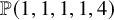
Proposition 3.1. Let F be a slope stable vector bundle on C of rank r, slope $\mu $
. Put
$\mu $
. Put $t:=\mu /12$
. Assume that
$t:=\mu /12$
. Assume that $t \in [0, 1/2] \cup [3/2, 2]$
. The following inequalities hold:
$t \in [0, 1/2] \cup [3/2, 2]$
. The following inequalities hold:
-
1. When
$t \in [0, 1/6)$
, we have
$h^0(F)/r \leq \frac {12t+24}{25}$
. -
2. When
$t \in [1/6, 1/4)$
, we have
$h^0(F)/r \leq \max \left \{ \frac {8t+8}{9}, \frac {10}{19}t+\frac {145}{152} \right \}$
. -
3. When
$t \in [1/4, 1/2]$
, we have
$h^0(F)/r \leq \max \left \{ 4t, \frac {33}{38}t+\frac {69}{76} \right \}$
. -
4. When
$t \in [3/2, 11/6]$
, we have
$h^0(F)/r \leq \max \left \{ 4t, \frac {231}{32}t-\frac {375}{64} \right \}$
. -
5. When
$t \in (11/6, \sqrt {14}/2]$
, we have
$h^0(F)/r \leq \frac {233t-191}{32}$
. -
6. When
$t \in [\sqrt {14}/2, 23/12]$
, we have
$h^0(F)/r \leq \frac {192t-168}{25}$
. -
7. When
$t \in [23/12, 2]$
, we have
$h^0(F)/r \leq 12t-15$
.


Figure 2 below indicates how the inequalities in Proposition 3.1 look like.
Remark 3.2. The parameter $t=\mu /12$
naturally appears as the BN slope of the sheaf
$t=\mu /12$
naturally appears as the BN slope of the sheaf $\iota _*F$
, where
$\iota _*F$
, where $\iota \colon C \hookrightarrow S$
is an embedding. Indeed, we have
$\iota \colon C \hookrightarrow S$
is an embedding. Indeed, we have $\nu _{BN}(\iota _*F)=t-3$
, as we will see in the proof of Lemma 3.7 below.
$\nu _{BN}(\iota _*F)=t-3$
, as we will see in the proof of Lemma 3.7 below.
It is also compatible with the slope function on T in the following sense. For a vector bundle F on T, we have $t(F|_C)=\mu _{H_T}(F)$
.
$t(F|_C)=\mu _{H_T}(F)$
.

Figure 2 The strong Clifford type bounds on C.
Our strategy of the proof of Proposition 3.1 is to use Bridgeland stability conditions on the surface S, with the following three steps.
-
1. Regard F as a torsion sheaf
$\iota _{*}F \in \operatorname {\mathrm {Coh}}(S)$
, which is
$\nu _{0, \alpha }$
-stable for
$\alpha \gg 0$
. -
2. Estimate the first possible wall for
$\iota _{*}F$
on the line
$\beta =0$
in
$(\alpha , \beta )$
plane, using the stronger form of the BG inequality on S. -
3. Bound global sections of BN-stable objects on S.


We define a function $\Upsilon $
on
$\Upsilon $
on $\mathbb {R}$
as
$\mathbb {R}$
as
 $$\begin{align*}\Upsilon(x):= \begin{cases} \frac{1}{2}x^2-\frac{1}{2}(1-\{x\})^2 & (\{x\} \in (0, 1/2]) \\ \frac{1}{2}x^2-\frac{1}{2}\{x\}^2 & (\{x\} \in [1/2, 1)) \\ \frac{1}{2}x^2 & (\{x\}=0). \end{cases} \end{align*}$$
Here, $\{x\}$
denotes the fractional part of
$\{x\}$
denotes the fractional part of $x \in \mathbb {R}$
. See Figure 3 above for the shape of
$x \in \mathbb {R}$
. See Figure 3 above for the shape of $\Upsilon $
. The following stronger BG inequality on the quadric surface
$\Upsilon $
. The following stronger BG inequality on the quadric surface $S \cong \mathbb {P}^1 \times \mathbb {P}^1$
is well-known. We include a proof here since it demonstrates the technique which we will frequently use in this section.
$S \cong \mathbb {P}^1 \times \mathbb {P}^1$
is well-known. We include a proof here since it demonstrates the technique which we will frequently use in this section.

Figure 3 The strong BG inequality $\Upsilon $
(red curve) on the quadric surface. Blue lines show the modified curve
$\Upsilon $
(red curve) on the quadric surface. Blue lines show the modified curve $\widetilde {\Upsilon }$
.
$\widetilde {\Upsilon }$
.
Lemma 3.3. Let F be a slope semistable torsion free sheaf on S. Then we have an inequality
 $$ \begin{align} \frac{\operatorname{\mathrm{ch}}_{2}(F)}{H^2\operatorname{\mathrm{ch}}_{0}(F)} \leq \Upsilon\left(\mu_H(F) \right). \end{align} $$
Proof. Since we have $\Upsilon (x+1)=\Upsilon (x)+x+1/2$
, the claim is invariant under tensoring with the line bundle
$\Upsilon (x+1)=\Upsilon (x)+x+1/2$
, the claim is invariant under tensoring with the line bundle $\mathcal {O}_S(H)$
. Hence, we may assume
$\mathcal {O}_S(H)$
. Hence, we may assume $\mu _H(F) \in (0, 1)$
. By the stability of F and the Serre duality, we have
$\mu _H(F) \in (0, 1)$
. By the stability of F and the Serre duality, we have
 $$\begin{align*}\hom(\mathcal{O}(1), F)=0, \quad \operatorname{\mathrm{ext}}^2(\mathcal{O}(1), F)=\hom(F, \mathcal{O}(-1))=0 \end{align*}$$
and hence $0 \geq -\operatorname {\mathrm {ext}}^1\left (\mathcal {O}(1), F \right ) =\chi \left (\mathcal {O}(1), F \right )$
. By computing the right-hand side using the Riemann–Roch theorem, we get the inequality
$0 \geq -\operatorname {\mathrm {ext}}^1\left (\mathcal {O}(1), F \right ) =\chi \left (\mathcal {O}(1), F \right )$
. By computing the right-hand side using the Riemann–Roch theorem, we get the inequality
 $$\begin{align*}\frac{\operatorname{\mathrm{ch}}_{2}(F)}{H^2\operatorname{\mathrm{ch}}_{0}(F)} \leq 0. \end{align*}$$
On the other hand, again by the stability of F and the Serre duality, we also have
 $$\begin{align*}\hom(F, \mathcal{O})=0, \quad \operatorname{\mathrm{ext}}^2(F, \mathcal{O})=\hom(\mathcal{O}, F(-2))=0, \end{align*}$$
which imply the inequality $0 \geq -\operatorname {\mathrm {ext}}^1(F, \mathcal {O})=\chi (F, \mathcal {O})$
. Hence, we obtain
$0 \geq -\operatorname {\mathrm {ext}}^1(F, \mathcal {O})=\chi (F, \mathcal {O})$
. Hence, we obtain
 $$\begin{align*}\frac{\operatorname{\mathrm{ch}}_2(F)}{H^2\operatorname{\mathrm{ch}}_0(F)} \leq \mu_H(F)-\frac{1}{2}. \end{align*}$$
Taking the minimum, the inequality (3) holds.
Remark 3.4. In [Reference RudakovRud94], Rudakov proved an inequality stronger than equation (3). However, our inequality is already optimal at $\mu _H=1/2$
(consider
$\mu _H=1/2$
(consider $F=\mathcal {O}_S(1, 0)$
). Because of this fact, we cannot improve our inequality in Theorem 1.1 at
$F=\mathcal {O}_S(1, 0)$
). Because of this fact, we cannot improve our inequality in Theorem 1.1 at $\mu _H=1/2$
, even if we use the result in [Reference RudakovRud94].
$\mu _H=1/2$
, even if we use the result in [Reference RudakovRud94].
We define a function $\widetilde {\Upsilon } \colon \mathbb {R} \to \mathbb {R}$
as
$\widetilde {\Upsilon } \colon \mathbb {R} \to \mathbb {R}$
as
 $$\begin{align*}\widetilde{\Upsilon}(x):= \begin{cases} \Upsilon(x) & (|x| \in [0, 1]) \\ \max\left\{ \Upsilon(x), \frac{1}{2} \lfloor |x| \rfloor x \right\} & (|x| \geq 1). \end{cases} \end{align*}$$
Here, $\lfloor |x| \rfloor $
denotes the integral part of the absolute value of a real number
$\lfloor |x| \rfloor $
denotes the integral part of the absolute value of a real number $x \in \mathbb {R}$
. Note that the function
$x \in \mathbb {R}$
. Note that the function $\widetilde {\Upsilon }$
is star-shaped and we have
$\widetilde {\Upsilon }$
is star-shaped and we have $\Upsilon (x) \leq \widetilde {\Upsilon }(x)$
for all
$\Upsilon (x) \leq \widetilde {\Upsilon }(x)$
for all $x \in \mathbb {R}$
; see Figure 3.
$x \in \mathbb {R}$
; see Figure 3.
We have the following consequences of Lemma 3.3.
Lemma 3.5. The following statements hold:
-
1. Fix a positive real number
$\alpha>0$
. Let
$F \in \operatorname {\mathrm {Coh}}^0(S)$
be a
$\nu _{0, \alpha }$
-semistable object with
$\operatorname {\mathrm {ch}}_0(F) \neq 0$
. Then the Chern character of F satisfies the inequality (4)
$$ \begin{align} \frac{\operatorname{\mathrm{ch}}_{2}(F)}{H^2\operatorname{\mathrm{ch}}_{0}(F)} \leq \widetilde{\Upsilon}\left(\mu_H(F) \right). \end{align} $$
-
2. For all real numbers
$\beta , \alpha \in \mathbb {R}$
with
$\alpha> \Upsilon (\beta )$
, the pair
$\left (Z_{\beta , \alpha }, \operatorname {\mathrm {Coh}}^\beta (S) \right )$
defines a stability condition on
$D^b(S)$
. Here, the group homomorphism
$Z_{\beta , \alpha } \colon K(S) \to \mathbb {C}$
is defined as
$$\begin{align*}Z_{\beta, \alpha}:=-\operatorname{\mathrm{ch}}_2+\alpha H^2\operatorname{\mathrm{ch}}_0 +i\left(H\operatorname{\mathrm{ch}}_1-\beta H^2\operatorname{\mathrm{ch}}_0 \right). \end{align*}$$


Proof.
-
(1) The first assertion follows from Lemma 3.3 and Proposition 2.5.
-
(2) For the second assertion, we can apply the arguments in [Reference Arcara and BertramAB13, Reference BridgelandBri08] by replacing the classical BG inequality with the stronger one, equation (3).
In the next two lemmas, we control the position of the first possible wall for $\iota _*F$
, where F is a stable bundle on C, and then bound the slopes of the Harder–Narasimhan (HN) factors of
$\iota _*F$
, where F is a stable bundle on C, and then bound the slopes of the Harder–Narasimhan (HN) factors of $\iota _*F$
with respect to BN stability.
$\iota _*F$
with respect to BN stability.
Lemma 3.6. Let F be a slope stable vector bundle on C with rank r, slope $\mu $
. Let
$\mu $
. Let $(\beta _1, \alpha _1), (\beta _2, \alpha _2)$
,
$(\beta _1, \alpha _1), (\beta _2, \alpha _2)$
, $\beta _1 < 0 < \beta _2$
, be the end points of a wall for
$\beta _1 < 0 < \beta _2$
, be the end points of a wall for $\iota _*F$
with respect to
$\iota _*F$
with respect to $\nu _{\beta , \alpha }$
-stability. Then we have
$\nu _{\beta , \alpha }$
-stability. Then we have $\beta _2-\beta _1 \leq 6$
.
$\beta _2-\beta _1 \leq 6$
.
Proof. By the Grothendieck–Riemann–Roch theorem, we have
 $$ \begin{align} \operatorname{\mathrm{ch}}(\iota_{*}F)=(0, 6rH, r(\mu-36)). \end{align} $$
Suppose that there exists a positive integer $\alpha $
and a destabilizing sequence
$\alpha $
and a destabilizing sequence
 $$\begin{align*}0 \to F_{2} \to \iota_{*}F \to F_{1} \to 0 \end{align*}$$
in $\operatorname {\mathrm {Coh}}^0(S)$
for
$\operatorname {\mathrm {Coh}}^0(S)$
for $\nu _{0, \alpha }$
-stability. Denote by W the corresponding wall. Note that
$\nu _{0, \alpha }$
-stability. Denote by W the corresponding wall. Note that $F_2$
is a coherent sheaf. Let
$F_2$
is a coherent sheaf. Let $T \subset F_2$
be a torsion part, and put
$T \subset F_2$
be a torsion part, and put $Q:=F_2/T$
. We have the following diagram in the tilted category
$Q:=F_2/T$
. We have the following diagram in the tilted category $\operatorname {\mathrm {Coh}}^0(S)$
:
$\operatorname {\mathrm {Coh}}^0(S)$
:

By taking the $\operatorname {\mathrm {Coh}}(S)$
-cohomology of the bottom row in the above diagram, we get the exact sequence
$\operatorname {\mathrm {Coh}}(S)$
-cohomology of the bottom row in the above diagram, we get the exact sequence
 $$\begin{align*}0 \to Q/\mathcal{H}^{-1}(F_1) \to \iota_*F/T \to F_1 \to 0 \end{align*}$$
in $\operatorname {\mathrm {Coh}}(S)$
. In particular, the sheaf
$\operatorname {\mathrm {Coh}}(S)$
. In particular, the sheaf $Q/\mathcal {H}^{-1}(F_1)$
is scheme-theoretically supported on the curve C. Hence, we have a surjection
$Q/\mathcal {H}^{-1}(F_1)$
is scheme-theoretically supported on the curve C. Hence, we have a surjection $Q|_C \twoheadrightarrow Q/\mathcal {H}^{-1}(F_1)$
and so get an inequality
$Q|_C \twoheadrightarrow Q/\mathcal {H}^{-1}(F_1)$
and so get an inequality
 $$\begin{align*}6H^2\operatorname{\mathrm{ch}}_0(Q)=H\operatorname{\mathrm{ch}}_1(Q|_C) \geq H\operatorname{\mathrm{ch}}_1(Q/\mathcal{H}^{-1}(F_1)). \end{align*}$$
Note also that we have $\operatorname {\mathrm {ch}}_0(Q)=\operatorname {\mathrm {ch}}_0(\mathcal {H}^{-1}(F_1))$
. Now we have
$\operatorname {\mathrm {ch}}_0(Q)=\operatorname {\mathrm {ch}}_0(\mathcal {H}^{-1}(F_1))$
. Now we have
 $$ \begin{align} \begin{aligned} \mu_H(Q)-\mu_H(\mathcal{H}^{-1}(F_1)) =\frac{H\operatorname{\mathrm{ch}}_1(Q/\mathcal{H}^{-1}(F_1))}{H^2\operatorname{\mathrm{ch}}_0(Q)} \leq 6. \end{aligned} \end{align} $$
Now let $(\beta _1, \alpha _1), (\beta _2, \alpha _2)$
be the end points of the wall W with
$(\beta _1, \alpha _1), (\beta _2, \alpha _2)$
be the end points of the wall W with $\beta _1 < 0 < \beta _2$
. By Bertram’s nested wall theorem (see, e.g., [Reference LiLi19a, Lemma 2.9], [Reference MaciociaMaci14]), we know that for
$\beta _1 < 0 < \beta _2$
. By Bertram’s nested wall theorem (see, e.g., [Reference LiLi19a, Lemma 2.9], [Reference MaciociaMaci14]), we know that for $0 < \epsilon \ll 1$
, we have
$0 < \epsilon \ll 1$
, we have
 $$\begin{align*}Q \in \operatorname{\mathrm{Coh}}^{\beta_{2}-\epsilon}(S), \quad \mathcal{H}^{-1}(F_{1})[1] \in \operatorname{\mathrm{Coh}}^{\beta_{1}+\epsilon}(S), \end{align*}$$
which in particular imply
 $$\begin{align*}\mu_{H}(Q)> \beta_{2}-\epsilon, \quad \mu_{H}(\mathcal{H}^{-1}(F_{1})) \leq \beta_{1}+\epsilon. \end{align*}$$
Combining with the inequality (6), we have the desired inequality
 $$\begin{align*}\beta_{2}-\beta_{1} \leq 6.\\[-34pt] \end{align*}$$
Lemma 3.7. Let F be a slope stable vector bundle on C with rank r, slope $\mu \in (0, 24)$
. Let
$\mu \in (0, 24)$
. Let $t:=\mu /12$
. The following statements hold:
$t:=\mu /12$
. The following statements hold:
-
1. If
$t \in \left (0, 2-\frac {\sqrt {14}}{2} \right ]$
, then the sheaf
$\iota _*F$
is BN-stable. -
2. We have
$$\begin{align*}\nu^+_{BN}(\iota_*F) \leq \begin{cases} 1-\frac{1}{2t} & (t \in (2-\sqrt{14}/2, 1/2] \cup [3/2, \sqrt{14}/2]) \\ \frac{-9t+11}{-8t+7} & (t \in [\sqrt{14}/2, 23/12]) \\ 3t-5 & (t \in [23/12, 2]). \end{cases} \end{align*}$$
-
3. We have
$$\begin{align*}\nu^-_{BN}(\iota_*F) \geq \begin{cases} \frac{-5(2t-7)}{2(t-6)} & (t \in (2-\sqrt{14}/2, 1/2] \cup [3/2, 11/6] ) \\ -2 & (t \in [11/6, 2]). \end{cases} \end{align*}$$


Proof. Let W be a wall for $\iota _*F$
, and let
$\iota _*F$
, and let $(\beta _1, \alpha _1), (\beta _2, \alpha _2)$
be the end points of the wall W with
$(\beta _1, \alpha _1), (\beta _2, \alpha _2)$
be the end points of the wall W with $\beta _1 < 0 < \beta _2$
. Recall that the wall W is a line segment with slope
$\beta _1 < 0 < \beta _2$
. Recall that the wall W is a line segment with slope $\nu _{BN}(\iota _*F)=\mu /12-3=t-3$
(see equation (5) for the second equality). Since the curve
$\nu _{BN}(\iota _*F)=\mu /12-3=t-3$
(see equation (5) for the second equality). Since the curve $\Upsilon $
is not continuous when
$\Upsilon $
is not continuous when $\beta \in \mathbb {Z}$
, the points
$\beta \in \mathbb {Z}$
, the points $(\beta _i, \alpha _i)$
are either on the graph of
$(\beta _i, \alpha _i)$
are either on the graph of $\Upsilon $
or on the vertical lines
$\Upsilon $
or on the vertical lines
 $$\begin{align*}L_n:=\left\{ (n, y) : \frac{n^2-1}{2} < y < \frac{n^2}{2} \right\}, \quad n \in \mathbb{Z}. \end{align*}$$
When both of the end points $(\beta _i, \alpha _i)$
are on the curve
$(\beta _i, \alpha _i)$
are on the curve $\Upsilon $
, we say that the wall W is of Type A; otherwise, we say it is of Type B.
$\Upsilon $
, we say that the wall W is of Type A; otherwise, we say it is of Type B.
First, assume that W is of Type A. By Lemma 3.6, we know that $\beta _2-\beta _1 \leq 6$
. Hence, the slope of the line through
$\beta _2-\beta _1 \leq 6$
. Hence, the slope of the line through $(\beta _{2}, \Upsilon (\beta _{2}))$
and
$(\beta _{2}, \Upsilon (\beta _{2}))$
and $(\beta _{2}-6, \Upsilon (\beta _{2}-6))$
is smaller than or equal to that of W, i.e.,
$(\beta _{2}-6, \Upsilon (\beta _{2}-6))$
is smaller than or equal to that of W, i.e., $\beta _{2}-3 \leq t-3$
. We conclude that every Type A wall is below the line
$\beta _{2}-3 \leq t-3$
. We conclude that every Type A wall is below the line $y=(t-3)(x-t)+\Upsilon (t)$
.
$y=(t-3)(x-t)+\Upsilon (t)$
.
On the other hand, for a given point $p=(\beta , \alpha ) \in L_n$
, let
$p=(\beta , \alpha ) \in L_n$
, let $W_p$
be the line passing through the point p with slope
$W_p$
be the line passing through the point p with slope $t-3$
. It is easy to compute the intersection points of
$t-3$
. It is easy to compute the intersection points of $W_p$
and
$W_p$
and $\Upsilon \cup \bigcup _{n \in \mathbb {Z}}L_n$
. Together with the constraint
$\Upsilon \cup \bigcup _{n \in \mathbb {Z}}L_n$
. Together with the constraint $\beta _2-\beta _1 \leq 6$
, we can find the first possible wall of Type B.
$\beta _2-\beta _1 \leq 6$
, we can find the first possible wall of Type B.
Using these observations, we can list up the equation of the first possible wall:
-
○ When
$t \in [0, 1/2]$
, the following is the first possible wall Note that, if
$$\begin{align*}y=(t-3)(x-t)+t-1/2. \end{align*}$$
$t \in [0, 2-\sqrt {14}/2]$
, it is negative at
$x=0$
, hence
$\iota _*F$
is BN stable.
-
○ When
$t \in [3/2, 2]$
, one of the following is the first possible wall The first one is the line passing through the points
$$\begin{align*}y=(t-3)(x-t)+t-1/2, \quad y=(t-3)(x+4)+8. \end{align*}$$
$(t, \Upsilon (t))$
and
$(t-6, \Upsilon (t-6))$
. The second one is the line with slope
$t-3$
, passing through the point
$(-4, \Upsilon (-4))$
. See Figure 4 below.Figure 4 The first possible wall L when
$t=3/2$
(left) and
$t=23/12$
(right).


Let L be the first possible wall described above, and let $(\beta _{\max }, \alpha _{\max })$
,
$(\beta _{\max }, \alpha _{\max })$
, $(\beta _{\min }, \alpha _{\min })$
be the intersection points of L with the curve
$(\beta _{\min }, \alpha _{\min })$
be the intersection points of L with the curve $\Upsilon $
with
$\Upsilon $
with $\beta _{\min }<\beta _{\max }$
. Then any wall W should be below the line L. Now consider the maximal destabilizing subobject
$\beta _{\min }<\beta _{\max }$
. Then any wall W should be below the line L. Now consider the maximal destabilizing subobject $E_{1} \subset \iota _{*}F$
with respect to the BN stability. We have three numerical constraints on
$E_{1} \subset \iota _{*}F$
with respect to the BN stability. We have three numerical constraints on $E_{1}$
:
$E_{1}$
:
-
○ Since
$\iota _{*}F$
is
$\nu _{\alpha , 0}$
-stable for
$\alpha $
sufficiently large, we have
$\operatorname {\mathrm {ch}}_{0}(E_{1})>0$
. -
○
$E_{1}$
satisfies the BG type inequality (4). -
○ The point
$p_{H}(E_{1})$
is below the line L.


Among all points satisfying the above three conditions, its slope becomes maximum at the point $(\alpha _{\max }, \beta _{\max })$
, hence we get the bound
$(\alpha _{\max }, \beta _{\max })$
, hence we get the bound
 $$\begin{align*}\nu_{BN}(E_{1}) \leq \frac{\alpha_{\max}}{\beta_{\max}}. \end{align*}$$
Now the straightforward computation shows the result. Similarly, we can get the bound $\nu ^-_{BN}(\iota _{*}F) \geq \alpha _{\min }/\beta _{\min }$
.
$\nu ^-_{BN}(\iota _{*}F) \geq \alpha _{\min }/\beta _{\min }$
.
The following lemma gives the upper bound on the number of global sections for BN stable objects.
Lemma 3.8. Let $F \in \operatorname {\mathrm {Coh}}^0(S)$
be a BN stable object. Then the following inequalities hold:
$F \in \operatorname {\mathrm {Coh}}^0(S)$
be a BN stable object. Then the following inequalities hold:
-
○ When
$-1 < \nu _{BN}(F) < +\infty $
, we have
$$\begin{align*}\hom(\mathcal{O}_{S}, F) = \operatorname{\mathrm{ch}}_{0}(F) + H\operatorname{\mathrm{ch}}_{1}(F) + \operatorname{\mathrm{ch}}_{2}(F). \end{align*}$$
-
○ When
$\nu _{BN}(E) \in (-n-1, -n)$
,
$n \in \mathbb {Z}_{>0}$
, we have
$$\begin{align*}\hom(\mathcal{O}_{S}, F) \leq \operatorname{\mathrm{ch}}_{0}(F) + \frac{1}{2n+1}H\operatorname{\mathrm{ch}}_{1}(F) + \frac{1}{(2n+1)^2}\operatorname{\mathrm{ch}}_{2}(F). \end{align*}$$
-
○ When
$\nu _{BN}(E)=-n$
,
$n \in \mathbb {Z}_{>0}$
, we have
$$\begin{align*}\hom(\mathcal{O}_S, F) \leq \operatorname{\mathrm{ch}}_0(F)+\frac{1}{4n}H\operatorname{\mathrm{ch}}_1(F). \end{align*}$$


Proof. First, assume that $\nu _{BN}(F)> -1$
. Noting
$\nu _{BN}(F)> -1$
. Noting $\nu _{BN}(\mathcal {O}_S[1])=+\infty $
and
$\nu _{BN}(\mathcal {O}_S[1])=+\infty $
and $\nu _{BN}(\mathcal {O}_{S}(-2)[1])=-1$
, we have the following vanishings for any
$\nu _{BN}(\mathcal {O}_{S}(-2)[1])=-1$
, we have the following vanishings for any $i \geq 0$
:
$i \geq 0$
:
 $$ \begin{align*} &\hom(\mathcal{O}_{S}, F[1+i])=\hom(F, \mathcal{O}_{S}(-2)[1-i])=0, \\ &\hom(\mathcal{O}_{S}, F[-1-i])=\hom(\mathcal{O}_{S}[1+i], F)=0. \end{align*} $$
Hence, by the Riemann–Roch, we get
 $$ \begin{align*} \hom(\mathcal{O}_{S}, F)=\chi(F) &=\int_{S}\operatorname{\mathrm{ch}}(F). (1, H, 1) \\ &=\operatorname{\mathrm{ch}}_{0}(F) + H\operatorname{\mathrm{ch}}_{1}(F) +\operatorname{\mathrm{ch}}_{2}(F). \end{align*} $$
Next, consider the case $\nu _{BN}(E) \in (-n-1, -n)$
,
$\nu _{BN}(E) \in (-n-1, -n)$
, $n \in \mathbb {Z}_{>0}$
. Let
$n \in \mathbb {Z}_{>0}$
. Let
 $$\begin{align*}(x_{F}, y_{F}):=p_{H}(F) =\left( \frac{H\operatorname{\mathrm{ch}}_{1}(F)}{H^2\operatorname{\mathrm{ch}}_{0}(F)}, \frac{\operatorname{\mathrm{ch}}_{2}(F)}{H^2\operatorname{\mathrm{ch}}_{0}(F)} \right). \end{align*}$$
Since we assumed $y_{F}/x_{F}=\nu _{BN}(F) \leq -1<0$
, the line through
$y_{F}/x_{F}=\nu _{BN}(F) \leq -1<0$
, the line through $(0, 0)$
and
$(0, 0)$
and $(x_{F}, y_{F})$
intersects with the region
$(x_{F}, y_{F})$
intersects with the region $y \geq 1/2x^2, x<0$
.
$y \geq 1/2x^2, x<0$
.
Take such a point $(\beta , \alpha )$
. Then we know that the objects
$(\beta , \alpha )$
. Then we know that the objects $F, \mathcal {O}_S \in \operatorname {\mathrm {Coh}}^\beta (S)$
are
$F, \mathcal {O}_S \in \operatorname {\mathrm {Coh}}^\beta (S)$
are $\nu _{\beta , \alpha }$
-semistable with
$\nu _{\beta , \alpha }$
-semistable with
 $$\begin{align*}\nu_{\beta, \alpha}(F) =\nu_{\beta, \alpha}(\mathcal{O}_{S}) =\alpha/\beta=\nu_{BN}(F). \end{align*}$$
Let us consider the exact triangle
 $$\begin{align*}\operatorname{\mathrm{Hom}}(\mathcal{O}_{S}, F) \otimes \mathcal{O}_{S} \xrightarrow{ev} F \to \widetilde{F}:=\operatorname{\mathrm{Cone}}(ev). \end{align*}$$
Since the only Jordan–Hölder factor of $\operatorname {\mathrm {Hom}}(\mathcal {O}_S, F) \otimes \mathcal {O}_S$
with respect to
$\operatorname {\mathrm {Hom}}(\mathcal {O}_S, F) \otimes \mathcal {O}_S$
with respect to $\nu _{\beta , \alpha }$
-stability is
$\nu _{\beta , \alpha }$
-stability is $\mathcal {O}_S$
, the evaluation map
$\mathcal {O}_S$
, the evaluation map $ev$
must be injective in the category
$ev$
must be injective in the category $\operatorname {\mathrm {Coh}}^{\beta }(S)$
. Hence, it follows that
$\operatorname {\mathrm {Coh}}^{\beta }(S)$
. Hence, it follows that $\widetilde {F} \in \operatorname {\mathrm {Coh}}^{\beta }(S)$
, and it is
$\widetilde {F} \in \operatorname {\mathrm {Coh}}^{\beta }(S)$
, and it is $\nu _{\beta , \alpha }$
-semistable with
$\nu _{\beta , \alpha }$
-semistable with $\nu _{\beta , \alpha }(\widetilde {F}) =\nu _{\beta , \alpha }(F)=\nu _{BN}(F)$
. Now choose
$\nu _{\beta , \alpha }(\widetilde {F}) =\nu _{\beta , \alpha }(F)=\nu _{BN}(F)$
. Now choose $\beta $
sufficiently close to zero so that
$\beta $
sufficiently close to zero so that $\mathcal {O}_{S}(-2n)[1] \in \operatorname {\mathrm {Coh}}^{\beta }(S)$
. As before, we have the vanishing statements
$\mathcal {O}_{S}(-2n)[1] \in \operatorname {\mathrm {Coh}}^{\beta }(S)$
. As before, we have the vanishing statements
 $$ \begin{align*} &\hom(\mathcal{O}_{S}(-2n), \widetilde{F}[1+i]) =\hom(\widetilde{F}, \mathcal{O}_{S}(-(2n+2))[1-i])=0, \\ &\hom(\mathcal{O}_{S}(-2n), \widetilde{F}[-1-i]) =\hom(\mathcal{O}_{S}(-2n)[1+i], \widetilde{F})=0 \end{align*} $$
for $i \geq 0$
. Hence, we have
$i \geq 0$
. Hence, we have
 $$ \begin{align*} 0 &\leq \hom(\mathcal{O}_{S}(-2n), \widetilde{F}) \\ &=\chi(\mathcal{O}_{S}(-2n), \widetilde{F}) \\ &=\operatorname{\mathrm{ch}}_{2}(F)+(2n+1)H\operatorname{\mathrm{ch}}_{1}(F) +(2n+1)^2(\operatorname{\mathrm{ch}}_{0}(F)-\hom(\mathcal{O}_{S}, F)), \end{align*} $$
and so
 $$\begin{align*}\hom(\mathcal{O}_{S}, F) \leq \operatorname{\mathrm{ch}}_{0}(F)+\frac{H\operatorname{\mathrm{ch}}_{1}(F)}{2n+1} +\frac{\operatorname{\mathrm{ch}}_{2}(F)}{(2n+1)^2} \end{align*}$$
as required.
Finally, assume that $\nu _{BN}(F)=-n$
,
$\nu _{BN}(F)=-n$
, $n \in \mathbb {Z}_{>0}$
. Then the same argument shows that
$n \in \mathbb {Z}_{>0}$
. Then the same argument shows that $\chi (\mathcal {O}_S(-2n+1), \widetilde {F}) \geq 0$
, and we get the inequality
$\chi (\mathcal {O}_S(-2n+1), \widetilde {F}) \geq 0$
, and we get the inequality
 $$\begin{align*}\hom(\mathcal{O}_S, F) \leq \operatorname{\mathrm{ch}}_0(F)+\frac{H\operatorname{\mathrm{ch}}_1(F)}{2n}+\frac{\operatorname{\mathrm{ch}}_2(F)}{(2n)^2} =\operatorname{\mathrm{ch}}_0(F)+\frac{1}{4n}H\operatorname{\mathrm{ch}}_{1}(F).\\[-40pt] \end{align*}$$
Let us define a function $\Omega \colon \mathbb {R} \times \mathbb {R}_{>0} \to \mathbb {R}_{>0}$
as
$\Omega \colon \mathbb {R} \times \mathbb {R}_{>0} \to \mathbb {R}_{>0}$
as
 $$\begin{align*}\Omega(x, y):= \begin{cases} y+x & (x/y> -1) \\ \frac{y}{2n+1}+\frac{x}{(2n+1)^2} & (x/y \in (-n-1, -n), n \in \mathbb{Z}_{>0}) \\ \frac{1}{4n}y & (x/y=-n, n \in \mathbb{Z}_{>0}). \end{cases} \end{align*}$$
Lemma 3.9. Let $O \in \mathbb {R}^2$
be the origin, and let
$O \in \mathbb {R}^2$
be the origin, and let $P=(x_p, y_p), Q=(x_q, y_q) \in \mathbb {R} \times \mathbb {R}_{>0}$
be points satisfying
$P=(x_p, y_p), Q=(x_q, y_q) \in \mathbb {R} \times \mathbb {R}_{>0}$
be points satisfying $x_p/y_p < x_q/y_q$
and
$x_p/y_p < x_q/y_q$
and $y_p> y_q$
.
$y_p> y_q$
.
Among all the sequences $O=P_0, P_1, \cdots , P_{m-1}, P_m=P$
of points in the triangle
$O=P_0, P_1, \cdots , P_{m-1}, P_m=P$
of points in the triangle $OPQ$
such that
$OPQ$
such that $P_0P_1 \cdots P_m$
form convex polygons, the sum
$P_0P_1 \cdots P_m$
form convex polygons, the sum
 $$\begin{align*}\sum_{i=1}^m \Omega(\overrightarrow{P_{i-1}P_i}) \end{align*}$$
can achieve the maximum only when $m \leq 2$
.
$m \leq 2$
.
Moreover, when $m=2$
, the point
$m=2$
, the point $P_1=(x_1, y_1)$
can be chosen to satisfy one of the following conditions:
$P_1=(x_1, y_1)$
can be chosen to satisfy one of the following conditions:
-
○
$P_1=Q$
, -
○
$P_1$
is on the line segment
$OQ$
(resp.
$PQ$
) such that the slope of
$P_1P$
(resp.
$OP_1$
) is
$-1/n$
for some
$n \in \mathbb {Z}_{>0}$
. -
○ The lines
$OP_1$
and
$P_1P$
have slopes
$-1/m, -1/n$
for some integers
$m, n \in \mathbb {Z}_{>0}$
.


Proof. The proof is elementary and almost identical with that of [Reference LiLi19a, Lemma 4.11]. The key observations are the following:
-
○ The function
$\Omega $
is linear with respect to both variables x and y as long as the slope
$x/y$
is fixed. -
○ The function
$\Omega $
is upper semicontinuous.


We refer to [Reference LiLi19a, Lemma 4.11] for the details.
Now we can prove Proposition 3.1.
Proof of Proposition 3.1
Let F be a slope stable vector bundle on C of rank r and slope $\mu $
. Let
$\mu $
. Let
 $$\begin{align*}0=E_{0} \subset E_{1} \subset \cdots \subset E_{m}=\iota_{*}F \end{align*}$$
be the HN filtration with respect to the BN stability, and define $P_{i}:=(\operatorname {\mathrm {ch}}_{2}(E_{i}), H\operatorname {\mathrm {ch}}_{1}(E_{i}))$
. We have an inequality
$P_{i}:=(\operatorname {\mathrm {ch}}_{2}(E_{i}), H\operatorname {\mathrm {ch}}_{1}(E_{i}))$
. We have an inequality
 $$ \begin{align} h^0(F) \leq \sum_{i=1}^m \Omega(\overrightarrow{P_{i-1}P_{i}}) \end{align} $$
by Lemma 3.8 (cf. [Reference LiLi19a, Equation (21)]). We will bound the RHS in the above inequality. Let us put
 $$\begin{align*}P=(x_p, y_p):=(\operatorname{\mathrm{ch}}_2(\iota_{*}F), H\operatorname{\mathrm{ch}}_{1}(\iota_{*}F)) =(r(\mu-36), 12r), \end{align*}$$
and $Q=(x_q, y_q)$
to be a point such that
$Q=(x_q, y_q)$
to be a point such that $x_q/y_q$
is the upper bound for
$x_q/y_q$
is the upper bound for $\nu ^+_{BN}(\iota _{*}F)$
, and
$\nu ^+_{BN}(\iota _{*}F)$
, and $(x_p-x_q)/(y_p-y_q)$
is the lower bound for
$(x_p-x_q)/(y_p-y_q)$
is the lower bound for $\nu ^-_{BN}(\iota _{*}F)$
, given in Lemma 3.7. We know that the HN polygon of
$\nu ^-_{BN}(\iota _{*}F)$
, given in Lemma 3.7. We know that the HN polygon of $\iota _{*}F$
with respect to the BN stability is inside the triangle
$\iota _{*}F$
with respect to the BN stability is inside the triangle $OPQ$
. Hence, by Lemma 3.9, we may assume
$OPQ$
. Hence, by Lemma 3.9, we may assume $m=2$
and the point
$m=2$
and the point $P_1$
satisfies one of the following conditions:
$P_1$
satisfies one of the following conditions:
-
○
$P_1=Q$
, -
○
$P_1$
is on the line segment
$OQ$
(resp.
$PQ$
) such that the slope of
$P_1P$
(resp.
$OP_1$
) is
$-1/n$
for some
$n \in \mathbb {Z}_{>0}$
. -
○ The lines
$OP_1$
and
$P_1P$
have slopes
$-1/m, -1/n$
for some integers
$m, n \in \mathbb {Z}_{>0}$
.


We now argue case by case.
(0) When $t \in (0, 2-\sqrt {14}/2]$
, the sheaf
$t \in (0, 2-\sqrt {14}/2]$
, the sheaf $\iota _*F$
is BN stable. The BN slope is
$\iota _*F$
is BN stable. The BN slope is $\nu _{BN}(\iota _*F)=t-3 \in (-3, -2)$
, hence by Lemma 3.8, we have
$\nu _{BN}(\iota _*F)=t-3 \in (-3, -2)$
, hence by Lemma 3.8, we have
 $$\begin{align*}h^0(F)/r \leq \frac{12}{5}+\frac{12(t-3)}{25} =\frac{12t+24}{25}. \end{align*}$$
(1) Assume $t \in (2-\sqrt {14}/2, 1/6)$
. By Lemma 3.7, we have
$t \in (2-\sqrt {14}/2, 1/6)$
. By Lemma 3.7, we have
-
○ The slope of
$\overrightarrow {OP}$
is
$\frac {1}{t-3} \in (-1/2, -1/3)$
, -
○ The slope of
$\overrightarrow {OQ}$
is
$\frac {2t}{2t-1} \in (-1/2, -1/3)$
. -
○ The slope of
$\overrightarrow {QP}$
is
$\frac {2(t-6)}{-5(2t-7)} \in (-1/2, -1/3)$
.


Hence, we may assume $P_1=Q=(x_q, y_q)$
. We get
$P_1=Q=(x_q, y_q)$
. We get
 $$ \begin{align*} h^0(F) &\leq \Omega(\overrightarrow{OQ})+\Omega(\overrightarrow{QP}) \\ &=\frac{y_q}{5}+\frac{x_q}{25} +\frac{y_p-y_q}{5}+\frac{x_p-x_q}{25} =\frac{12t+24}{25}r. \end{align*} $$
(2) Assume $t \in [1/6, 1/4)$
. Then the slopes of the triangle
$t \in [1/6, 1/4)$
. Then the slopes of the triangle $OPQ$
are the same as the case (1). The only difference is that the slope of
$OPQ$
are the same as the case (1). The only difference is that the slope of $\overrightarrow {OQ}$
sits inside the interval
$\overrightarrow {OQ}$
sits inside the interval $(-1, -1/2]$
, instead of
$(-1, -1/2]$
, instead of $(-1/2, -1/3)$
. Hence, we may take
$(-1/2, -1/3)$
. Hence, we may take $P_1$
as Q or the point A on the line segment
$P_1$
as Q or the point A on the line segment $QP$
with slope
$QP$
with slope $-1/2$
. The coordinates are given as
$-1/2$
. The coordinates are given as
 $$\begin{align*}Q=((2t-1)r, 2tr), \quad A=\left( \frac{24(2t^2-8t+1)}{-6t+11}r, \frac{12(2t^2-8t+1)}{-6t+11}r \right). \end{align*}$$
First, consider the case of $P_1=Q \neq A$
. We have
$P_1=Q \neq A$
. We have
 $$ \begin{align*} \Omega(\overrightarrow{OQ})+\Omega(\overrightarrow{QP}) &=\frac{y_q}{3}+\frac{x_q}{9} +\frac{y_p-y_q}{5}+\frac{x_p-x_q}{25} \\ &=\frac{8t+8}{9}r. \end{align*} $$
When $P_1=A$
, we have
$P_1=A$
, we have
 $$ \begin{align*} \Omega(\overrightarrow{OA})+\Omega(\overrightarrow{AP}) &=\frac{y_a}{8} +\frac{y_p-y_a}{5}+\frac{x_p-x_a}{25} \\ &=\frac{1}{200}y_a+\frac{12t+24}{25}r. \end{align*} $$
As a function on $t \in [1/6, 1/4]$
, we have an inequality
$t \in [1/6, 1/4]$
, we have an inequality
 $$\begin{align*}y_a(t) \leq \left(\frac{176}{19}t -\frac{23}{19}\right)r \end{align*}$$
since the equality holds for $t=1/4, 1/6$
, and
$t=1/4, 1/6$
, and $y^{\prime \prime }_a(t)> 0$
for
$y^{\prime \prime }_a(t)> 0$
for $t < 11/6$
. Hence, we obtain
$t < 11/6$
. Hence, we obtain
 $$ \begin{align*} \Omega(\overrightarrow{OA})+\Omega(\overrightarrow{AP}) &\leq \frac{1}{200}\left( \frac{176}{19}t-\frac{23}{19} \right)r +\frac{12t+24}{25}r \\ &=\left(\frac{10}{19}t+\frac{145}{152}\right)r. \end{align*} $$
We conclude that
 $$\begin{align*}h^0(F)/r \leq \max\left\{ \frac{8t+8}{9}, \frac{10}{19}t+\frac{145}{152} \right\}. \end{align*}$$
(3) Assume $t \in [1/4, 1/2]$
. Again the only difference with the cases (1), (2) is that the slope of
$t \in [1/4, 1/2]$
. Again the only difference with the cases (1), (2) is that the slope of $OQ$
is smaller than or equal to
$OQ$
is smaller than or equal to $-1$
(or
$-1$
(or $+\infty $
when
$+\infty $
when $t=1/2$
) in the present case. Hence, we may choose
$t=1/2$
) in the present case. Hence, we may choose $P_1$
to be Q, or the points
$P_1$
to be Q, or the points $A, B$
on the line segment
$A, B$
on the line segment $QP$
with slope
$QP$
with slope $-1/2, -1$
, respectively. The coordinate of
$-1/2, -1$
, respectively. The coordinate of $Q, A$
are the same as in equation (2), and we have
$Q, A$
are the same as in equation (2), and we have
 $$\begin{align*}B=(x_b, y_b)=\left( -\frac{12(2t^2-8t+1)}{8t-23}r, \frac{12(2t^2-8t+1)}{8t-23}r \right). \end{align*}$$
We get
 $$ \begin{align*} &\Omega(\overrightarrow{OQ})+\Omega(\overrightarrow{QP}) =y_q+x_q +\frac{y_p-y_q}{5}+\frac{x_p-x_q}{25} =4tr, \\ &\Omega(\overrightarrow{OB})+\Omega(\overrightarrow{BP}) =\frac{1}{4}y_b +\frac{y_p-y_b}{5}+\frac{x_p-x_b}{25} =\frac{9}{100}y_b+\frac{12t+24}{25}r. \end{align*} $$
As a function of $t \in [1/4, 1/2]$
, we have the inequality
$t \in [1/4, 1/2]$
, we have the inequality
 $$\begin{align*}y_b(t) \leq \left(\frac{82}{19}t-\frac{11}{19} \right)r \end{align*}$$
and hence
 $$\begin{align*}\Omega(\overrightarrow{OB})+\Omega(\overrightarrow{BP}) \leq \frac{33}{38}tr+\frac{69}{76}r. \end{align*}$$
We can directly compute that
 $$\begin{align*}\Omega(\overrightarrow{OA})+\Omega(\overrightarrow{AP}) =\frac{1}{200}y_a+\frac{12t+24}{25} \leq \frac{33}{38}tr+\frac{69}{76}r. \end{align*}$$
We conclude that
 $$\begin{align*}h^0(F)/r \leq \max\left\{ 4t, \frac{33}{38}t+\frac{69}{76} \right\}. \end{align*}$$
(4) Assume $t \in [3/2, 11/6]$
. In this case, we have
$t \in [3/2, 11/6]$
. In this case, we have
-
○ The slope of
$\overrightarrow {OP}$
is
$\frac {1}{t-3} \in (-1, -1/2)$
, -
○ The slope of
$\overrightarrow {OQ}$
is
$\frac {2t}{2t-1}>0$
, -
○ The slope of
$\overrightarrow {QP}$
is
$\frac {2(t-6)}{-5(2t-7)} \in [-1/2, -1/3)$
.


There are four choices of the point $P_1$
, say
$P_1$
, say $Q, A, B, C$
, where A is the point on the line
$Q, A, B, C$
, where A is the point on the line $PQ$
with slope
$PQ$
with slope $-1$
, B is the point on the line
$-1$
, B is the point on the line $OQ$
such that the slope of
$OQ$
such that the slope of $BP$
is
$BP$
is $-1/2$
and C is the intersection point of two lines
$-1/2$
and C is the intersection point of two lines $OA$
and
$OA$
and $BP$
. Explicitly, we have
$BP$
. Explicitly, we have
 $$ \begin{align*} &Q=\left((2t-1)r, 2tr \right), \quad A=\left( -\frac{12(2t^2-8t+1)}{8t-23}r, \frac{12(2t^2-8t+1)}{8t-23}r \right), \\ &B=\left( \frac{12(2t-1)(t-1)}{6t-1}r, \frac{24t(t-1)}{6t-1}r \right), \quad C=\left( -12(t-1)r, 12(t-1)r \right). \end{align*} $$
Hence, we get
 $$ \begin{align*} &\Omega(\overrightarrow{OQ})+\Omega(\overrightarrow{QP}) =\frac{4}{5}y_q+\frac{24}{25}x_q+\frac{12t+24}{25}r =4tr, \\ &\Omega(\overrightarrow{OA})+\Omega(\overrightarrow{AP}) =\frac{9}{100}y_a+\frac{12t+24}{25}r, \\ &\Omega(\overrightarrow{OB})+\Omega(\overrightarrow{BP}) =y_b+x_b+\frac{y_p-y_b}{8} =\frac{7}{8}y_b+x_b+\frac{3}{2}r, \\ &\Omega(\overrightarrow{OC})+\Omega(\overrightarrow{CP}) =\frac{y_c}{4}+\frac{y_p-y_c}{8} =\frac{3}{2}tr. \end{align*} $$
First, we can show that
 $$\begin{align*}\frac{9}{100}y_a < \frac{4}{5}y_q+\frac{24}{25}x_q \end{align*}$$
for $t \in [3/2, 11/6]$
. On the other hand, it is easy to see
$t \in [3/2, 11/6]$
. On the other hand, it is easy to see
 $$\begin{align*}\Omega(\overrightarrow{OC})+\Omega(\overrightarrow{CP}) \leq \Omega(\overrightarrow{OB})+\Omega(\overrightarrow{BP}) =\frac{90t^2-96t+21}{2(6t-1)}r \leq \left(\frac{231}{32}t-\frac{375}{64} \right)r. \end{align*}$$
Hence, we can conclude that
 $$\begin{align*}h^0(F)/r \leq \max \left\{ 4t, \frac{231}{32}t-\frac{375}{64} \right\}. \end{align*}$$
(5) Assume $t \in (11/6, \sqrt {14}/2]$
. Then we have
$t \in (11/6, \sqrt {14}/2]$
. Then we have
-
○ The slope of
$\overrightarrow {OP}$
is
$\frac {1}{t-3} \in (-1, -1/2)$
, -
○ The slope of
$\overrightarrow {OQ}$
is
$\frac {2t}{2t-1}>0$
, -
○ The slope of
$\overrightarrow {QP}$
is
$-1/2$
.


Hence, we can choose the point $P_1$
to be B or C appeared in the case (4) above. For
$P_1$
to be B or C appeared in the case (4) above. For $t \in [11/6, \sqrt {14}/2]$
, we have
$t \in [11/6, \sqrt {14}/2]$
, we have
 $$\begin{align*}\Omega(\overrightarrow{OC})+\Omega(\overrightarrow{CP}) \leq \Omega(\overrightarrow{OB})+\Omega(\overrightarrow{BP}) =\frac{90t^2-96t+21}{2(6t-1)}r \leq \left(\frac{233}{32}t-\frac{191}{32} \right)r. \end{align*}$$
(6) Assume $t \in [\sqrt {14}/2, 23/12]$
. In this case, we have
$t \in [\sqrt {14}/2, 23/12]$
. In this case, we have
-
○ The slope of
$\overrightarrow {OP}$
is
$\frac {1}{t-3} \in (-1, -1/2)$
, -
○ The slope of
$\overrightarrow {OQ}$
is
$\frac {8t-7}{9t-11}>0$
, -
○ The slope of
$\overrightarrow {QP}$
is
$-1/2$
.


We may choose the point $P_1$
as Q or A, where A is the point on the line
$P_1$
as Q or A, where A is the point on the line $PQ$
with slope
$PQ$
with slope $-1$
. Explicitly, we have
$-1$
. Explicitly, we have
 $$ \begin{align*} &Q=\left( \frac{12}{25}(9t-11)r, \frac{12}{25}(8t-7)r \right), \quad A=\left( -12(t-1)r, 12(t-1)r \right), \end{align*} $$
and hence
 $$ \begin{align*} &\Omega(\overrightarrow{OQ})+\Omega(\overrightarrow{QP}) =y_q+x_q+\frac{y_p-y_q}{8} =\frac{192t-168}{25}r, \\ &\Omega(\overrightarrow{OA})+\Omega(\overrightarrow{AP}) =\frac{y_a}{4}+\frac{y_p-y_a}{8} =\frac{3}{2}tr. \end{align*} $$
We can see that $\Omega (\overrightarrow {OQ})+\Omega (\overrightarrow {QP}) \geq \Omega (\overrightarrow {OA})+\Omega (\overrightarrow {AP})$
, hence we conclude that
$\Omega (\overrightarrow {OQ})+\Omega (\overrightarrow {QP}) \geq \Omega (\overrightarrow {OA})+\Omega (\overrightarrow {AP})$
, hence we conclude that
 $$\begin{align*}h^0(F)/r \leq \frac{192t-168}{25}. \end{align*}$$
(7) Assume $t \in [23/12, 2)$
. Then we have
$t \in [23/12, 2)$
. Then we have
-
○ The slope of
$\overrightarrow {OP}$
is
$\frac {1}{t-3} \in (-1, -1/2)$
, -
○ The slope of
$\overrightarrow {OQ}$
is
$\frac {1}{3t-5}>0$
, -
○ The slope of
$\overrightarrow {QP}$
is
$-1/2$
.


Hence, $P_{1}=Q$
or A, where A is the point on the line segment
$P_{1}=Q$
or A, where A is the point on the line segment $PQ$
with slope
$PQ$
with slope $-1$
, i.e.,
$-1$
, i.e.,
 $$\begin{align*}Q=((12t-20)r, 4r), \quad A=((-12t+12)r, (12t-12)r).\\[-15pt] \end{align*}$$
We can calculate as
 $$ \begin{align*} &\Omega(\overrightarrow{OQ})+\Omega(\overrightarrow{QP}) =\left(12t-15 \right)r, \\ &\Omega(\overrightarrow{OA})+\Omega(\overrightarrow{AP}) =\frac{3}{2}tr \end{align*} $$
hence taking the maximum, we conclude that
 $$\begin{align*}h^0(F)/r \leq 12t-15.\\[-36pt] \end{align*}$$
4 Stronger BG inequality
Using the Clifford type bound obtained in Proposition 3.1, we prove the following stronger version of the (classical) BG inequality on a triple cover CY3 $X:=X_6 \subset \mathbb {P}(1, 1, 1, 1, 2)$
.
$X:=X_6 \subset \mathbb {P}(1, 1, 1, 1, 2)$
.
Theorem 4.1. Let X be a triple cover CY3. Let $F \in D^b(X)$
be a
$F \in D^b(X)$
be a $\nu _{\alpha , 0}$
-semistable object for some
$\nu _{\alpha , 0}$
-semistable object for some $\alpha> 0$
, with
$\alpha> 0$
, with $\mu _H(F) \in [-1, 1]$
. Then we have the following inequality
$\mu _H(F) \in [-1, 1]$
. Then we have the following inequality
 $$ \begin{align} \frac{H\operatorname{\mathrm{ch}}_2(F)}{H^3\operatorname{\mathrm{ch}}_0(F)} \leq \Xi \left(\left|\mu_H(F) \right|\right),\\[-15pt]\nonumber \end{align} $$
where
 $$\begin{align*}\Xi(t):=\left\{ \begin{array}{ll} t^2-t & (t \in [0, 1/4]) \\ 3t/4-3/8 & (t \in [1/4, 1/2]) \\ t/4-1/8 & (t \in [1/2, 3/4]) \\ t^2-1/2 & (t \in [3/4, 1]). \end{array} \right.\\[-15pt] \end{align*}$$
Proof. Assume for contradiction that there is a tilt semistable object F violating the inequality (8). We may assume $\mu _H(F) \geq 0$
by replacing F with
$\mu _H(F) \geq 0$
by replacing F with $F^\vee $
if necessary. First, observe that the following conditions hold:
$F^\vee $
if necessary. First, observe that the following conditions hold:
-
○ Let
$p=(a, b)$
be an arbitrary point with
$a \in [0, 1], b>\Xi (a)$
, and take a real number
$\alpha>0$
(resp.
$\alpha '>1/2$
). Then the line segment connecting the points p and
$(0, \alpha )$
(resp.
$(1, \alpha ')$
) is above the graph of
$\Xi $
. -
○ Let L be the line through
$p_H(F)$
and
$p_H(F(-2H)[1])$
. Then L passes through points
$(0, \alpha _0), (-1, \alpha _0')$
with
$\alpha _0>0, \alpha _0' > 1/2$
. Putting
$(a, b):=p_H(F)$
, the conditions are equivalent to the inequalities
$$\begin{align*}b> a^2-a, \quad b > a^2-1/2.\\[-15pt] \end{align*}$$


Under these conditions, we can apply the arguments in [Reference LiLi19a, Proposition 5.2, Corollary 5.4]. As a result, by restricting to the surface $T=T_{2, 6} \subset X_{6}$
, we obtain a tilt-stable object F on T with
$T=T_{2, 6} \subset X_{6}$
, we obtain a tilt-stable object F on T with $\mu _H(F) \in (0, 1)$
and
$\mu _H(F) \in (0, 1)$
and
 $$ \begin{align} \frac{\operatorname{\mathrm{ch}}_2(F)}{H^2\operatorname{\mathrm{ch}}_0(F)}> \Xi \left(\frac{H\operatorname{\mathrm{ch}}_1(F)}{H^2\operatorname{\mathrm{ch}}_0(F)} \right). \end{align} $$
Furthermore, by the first paragraph in the proof of [Reference LiLi19a, Proposition 5.2], we may assume that
-
○
$\mu _{H_{T}}(F) \in (0, 1/2]$
, -
○ F is
$\mu _{H_{T}}$
-stable coherent sheaf, -
○
$F|_{C}, F^{\vee }(2H_{T})|_{C}$
are slope stable.


Using the Riemann–Roch and the vanishings
 $$\begin{align*}\hom(\mathcal{O}_{T}, F(-2H_{T}))=0=\hom(\mathcal{O}_{T}, F^{\vee}) \end{align*}$$
(both follows from slope stability of F and the assumption on its slope), we have
 $$ \begin{align} \begin{aligned} \operatorname{\mathrm{ch}}_{2}(F)-H_{T}\operatorname{\mathrm{ch}}_{1}(F)+11\operatorname{\mathrm{ch}}_{0}(F) &=\chi(F) \\ &\leq h^0(F|_C)+h^0(F^{\vee}(2H_{T})|_{C}). \end{aligned} \end{align} $$
Note that we have
 $$ \begin{align*} &\operatorname{\mathrm{ch}}(F |_C)=(\operatorname{\mathrm{ch}}_0(F), 2H\operatorname{\mathrm{ch}}_1(F)), \\ &\operatorname{\mathrm{ch}}(F^{\vee}(2H_{T})|_C)=(\operatorname{\mathrm{ch}}_0(F), 4H^2\operatorname{\mathrm{ch}}_0(F)-2H\operatorname{\mathrm{ch}}_1(F)). \end{align*} $$
Applying Proposition 3.1 to the RHS of equation (10), we get
 $$ \begin{align} \frac{\operatorname{\mathrm{ch}}_{2}(F)}{H^2\operatorname{\mathrm{ch}}_{0}(F)} \leq \begin{cases} -\frac{23}{25}\mu_H(F)-\frac{13}{75} & (\mu_H(F) \in (0, 1/12]) \\ -\frac{1}{5}\mu_H(F)-\frac{7}{30} & (\mu_{H}(F) \in [1/12, 2-\sqrt{14}/2]) \\ -\frac{641}{4800}\mu_H(F)-\frac{1157}{4800} & (\mu_{H}(F) \in [2-\sqrt{14}/2, 1/6)) \\ -\frac{421}{3648}\mu_H(F)-\frac{595}{2432} & (\mu_{H}(F) \in [1/6, 89/496]) \\ -\frac{95}{1728}\mu_H(F)-\frac{883}{3456} & (\mu_{H}(F) \in [89/496, 37/206]) \\ \frac{13}{27}\mu_H(F)-\frac{19}{54} & (\mu_{H}(F) \in [37/206, 1/4)) \\ \frac{109}{228}\mu_H(F)-\frac{53}{152} & (\mu_{H}(F) \in [1/4, 69/238]) \\ \mu_H(F)-\frac{1}{2} & (\mu_{H}(F) \in [69/238, 1/2]). \end{cases} \end{align} $$
In all cases, the inequalities (11) contradict the inequality (9).
5 The case of double cover
In this section, we consider the double cover X of $\mathbb {P}^3$
branched along a smooth hypersurface of degree
$\mathbb {P}^3$
branched along a smooth hypersurface of degree $8$
; X is another example of Calabi–Yau threefolds. As in the previous sections, we treat X as a weighted hypersurface in
$8$
; X is another example of Calabi–Yau threefolds. As in the previous sections, we treat X as a weighted hypersurface in $P=\mathbb {P}(1, 1, 1, 1, 4)$
of degree
$P=\mathbb {P}(1, 1, 1, 1, 4)$
of degree $8$
. Let
$8$
. Let
 $$\begin{align*}C_{2, 4, 8} \subset T_{2, 8} \subset X_8, \quad C_{2, 4, 8} \subset S_{2, 4} \end{align*}$$
be smooth $(2, 4, 8)$
-,
$(2, 4, 8)$
-, $(2, 8)$
-,
$(2, 8)$
-, $(2, 4)$
-complete intersections in P. The following is the list of their numerical invariants we need.
$(2, 4)$
-complete intersections in P. The following is the list of their numerical invariants we need.
-
○
$-K_P=8H$
,
$H_P^4=1/4$
, -
○
$g(C)=49$
, -
○
$S \cong \mathbb {P}^1 \times \mathbb {P}^1$
, -
○
$K_T=2H_T$
,
$H_T^2=4$
,
$\operatorname {\mathrm {td}}_T=(1, -H_T, 10)$
, -
○
$\operatorname {\mathrm {td}}_X=(1, 0, \frac {11}{6}H_X^2, 0)$
,
$H_X^3=2$
.


Remark 5.1. To make the surface S smooth, we take a $(2, 4)$
-complete intersection instead of a
$(2, 4)$
-complete intersection instead of a $(2, 2)$
-complete intersection.
$(2, 2)$
-complete intersection.
5.1 Clifford type bound
In this subsection, we will prove the Clifford type theorem for the curve $C=C_{2, 4, 8}$
, using the embedding
$C=C_{2, 4, 8}$
, using the embedding $\iota $
into the quadric surface
$\iota $
into the quadric surface $S \cong \mathbb {P}^1 \times \mathbb {P}^1$
.
$S \cong \mathbb {P}^1 \times \mathbb {P}^1$
.
Lemma 5.2. Let F be a slope stable vector bundle on C with rank r slope $\mu $
. Put
$\mu $
. Put $t:=\frac {\mu }{16}$
, and assume
$t:=\frac {\mu }{16}$
, and assume $t \in [0, 1/2] \cup [3/2, 2]$
. Then we have the following statements hold:
$t \in [0, 1/2] \cup [3/2, 2]$
. Then we have the following statements hold:
-
1. When
$t \in \left [0, \frac {5-\sqrt {23}}{2} \right ]$
, the sheaf
$\iota _*F$
is BN stable. -
2. We have
$$\begin{align*}\nu^+_{BN}(\iota_{*}F) \leq \begin{cases} 1-\frac{1}{2t} & (t \in [\frac{5-\sqrt{23}}{2}, 1/2] \cup [3/2, \frac{\sqrt{23}-1}{2}]) \\ \frac{-13t+16}{-12t+11} & (t \in [\frac{\sqrt{23}-1}{2}, 31/16]) \\ 4t-7 & (t \in [31/16, 2]). \end{cases} \end{align*}$$
-
3. We have
$$\begin{align*}\nu^-_{BN}(\iota_{*}F) \geq \begin{cases} \frac{-7(2t-9)}{2(t-8)} & (t \in (\frac{5-\sqrt{23}}{2}, 1/2] \cup [3/2, 15/8]) \\ -3 & (t \in [15/8, 2]). \end{cases} \end{align*}$$


Proof. The proof is almost identical to that of Lemma 3.7. Hence, we just give an outline of the proof. Let us consider the embedding $\iota \colon C \hookrightarrow S$
. For
$\iota \colon C \hookrightarrow S$
. For $F \in \operatorname {\mathrm {Coh}}(C)$
, we have
$F \in \operatorname {\mathrm {Coh}}(C)$
, we have $\operatorname {\mathrm {ch}}(\iota _*F)=(0, 8rH, r(\mu -64))$
. Let W be a wall for
$\operatorname {\mathrm {ch}}(\iota _*F)=(0, 8rH, r(\mu -64))$
. Let W be a wall for $\iota _*F$
with respect to the
$\iota _*F$
with respect to the $\nu _{\alpha , 0}$
-stability, and let
$\nu _{\alpha , 0}$
-stability, and let $\beta _1, \beta _2$
be the
$\beta _1, \beta _2$
be the $\beta $
-coordinates of the end points of the wall W with
$\beta $
-coordinates of the end points of the wall W with $\beta _1 < 0 < \beta _2$
. Then we can show that
$\beta _1 < 0 < \beta _2$
. Then we can show that $\beta _2-\beta _1 \leq 8$
. We have
$\beta _2-\beta _1 \leq 8$
. We have $\nu _{BN}(\iota _*F)=t-4$
, and we can get the bounds of the first possible wall as follows:
$\nu _{BN}(\iota _*F)=t-4$
, and we can get the bounds of the first possible wall as follows:
-
○ When
$t \in [0, 1/2]$
, the equation of the first possible wall is which is the line passing through the points
$$\begin{align*}y=(t-4)(x-t)+t-1/2, \end{align*}$$
$(t, \Upsilon (t)), (t-8, \Upsilon (t-8))$
. We can see that
$y(0) \leq 0$
for
$t \in [0, \frac {5-\sqrt {23}}{2}]$
, hence the sheaf
$\iota _*F$
is BN stable.
-
○ When
$t \in [3/2, 2]$
, we have two possibilities of the first wall: The first equation is the line passing through the points
$$\begin{align*}y=(t-4)(x-t)+t-1/2, \quad y=(t-4)(x+6)+18. \end{align*}$$
$(t, \Upsilon (t)), (t-8, \Upsilon (t-8))$
, and the second one is the line passing through the point
$(-6, \Upsilon (-6))$
with slope
$t-4$
.


As similar to Lemma 3.7, we get the bound on $\nu _{BN}^{\pm }(\iota _*F)$
by computing the end points of the first possible walls listed above.
$\nu _{BN}^{\pm }(\iota _*F)$
by computing the end points of the first possible walls listed above.
We get the following Clifford type bound:
Proposition 5.3. Let F be a slope stable vector bundle on C of rank r, slope $\mu \in (0, 8] \cup [24, 32)$
. Put
$\mu \in (0, 8] \cup [24, 32)$
. Put $t:=\mu /16$
. The following inequalities hold:
$t:=\mu /16$
. The following inequalities hold:
-
1. When
$t \in (0, 1/8)$
, we have
$h^0(F)/r \leq \frac {16(t+3)}{49}$
. -
2. When
$t \in [1/8, 1/6)$
, we have
$h^0(F)/r \leq \max \left \{ \frac {12t+24}{25}, \frac {85t}{246}+\frac {481}{492} \right \}$
. -
3. When
$t \in [1/6, 1/4)$
, we have
$h^0(F)/r \leq \max \left \{ \frac {8t+8}{9}, \frac {17t}{38}+\frac {147}{152} \right \}$
. -
4. When
$t \in [1/4, 1/2]$
, we have
$h^0(F)/r \leq \max \left \{ 4t, \frac {63t}{82}+\frac {153}{164} \right \}$
. -
5. When
$t \in [3/2, 15/8]$
, we have
$h^0(F)/r \leq 4t$
. -
6. When
$t \in (15/8, \frac {\sqrt {23}-1}{2}]$
, we have
$h^0(F)/r \leq \frac {133t-114}{18}$
. -
7. When
$t \in [\frac {\sqrt {23}-1}{2}, 31/16]$
, we have
$h^0(F)/r \leq \frac {236}{49}t-\frac {148}{21}$
. -
8. When
$t \in [31/16, 2)$
, we have
$h^0(F)/r \leq 16t-23$
.


Proof. As in the proof of Proposition 3.1, the problem is reduced to computing $\Omega (\overrightarrow {OP_1})+\Omega (\overrightarrow {P_1P})$
for appropriate candidate points
$\Omega (\overrightarrow {OP_1})+\Omega (\overrightarrow {P_1P})$
for appropriate candidate points $P_1$
in the triangle
$P_1$
in the triangle $OPQ$
. Here, the points
$OPQ$
. Here, the points $P, Q$
are defined as before, namely,
$P, Q$
are defined as before, namely, $P:=(\operatorname {\mathrm {ch}}_2(\iota _*F),H\operatorname {\mathrm {ch}}_1(\iota _*F))=(16(t-4)r, 16r)$
, and
$P:=(\operatorname {\mathrm {ch}}_2(\iota _*F),H\operatorname {\mathrm {ch}}_1(\iota _*F))=(16(t-4)r, 16r)$
, and $Q=(x_q, y_q)$
is the point such that
$Q=(x_q, y_q)$
is the point such that $x_q/y_q$
is the upper bound for
$x_q/y_q$
is the upper bound for $\nu ^+_{BN}(\iota _{*}F)$
, and
$\nu ^+_{BN}(\iota _{*}F)$
, and $(x_p-x_q)/(y_p-y_q)$
is the lower bound for
$(x_p-x_q)/(y_p-y_q)$
is the lower bound for $\nu ^-_{BN}(\iota _{*}F)$
, given in Lemma 5.2.
$\nu ^-_{BN}(\iota _{*}F)$
, given in Lemma 5.2.
(0) First, assume that $t \in \left [0, \frac {5-\sqrt {23}}{2} \right ]$
. In this case, the sheaf
$t \in \left [0, \frac {5-\sqrt {23}}{2} \right ]$
. In this case, the sheaf $\iota _*F$
is BN stable with BN slope
$\iota _*F$
is BN stable with BN slope $\nu _{BN}(\iota _*F)=t-4 \in (-4, -3)$
. Hence, we have
$\nu _{BN}(\iota _*F)=t-4 \in (-4, -3)$
. Hence, we have
 $$\begin{align*}h^0(F)/r \leq \frac{16}{7}+\frac{16(t-4)}{49} =\frac{16(t+3)}{49} \end{align*}$$
by Lemma 3.8.
(1) Assume $t \in \left [\frac {5-\sqrt {23}}{2}, \frac {1}{8} \right )$
. By Lemma 5.2, we have
$t \in \left [\frac {5-\sqrt {23}}{2}, \frac {1}{8} \right )$
. By Lemma 5.2, we have
-
○ The slope of
$\overrightarrow {OP}$
is
$\frac {1}{t-4} \in (-1/3, -1/4)$
, -
○ The slope of
$\overrightarrow {OQ}$
is
$\frac {2t}{2t-1} \in (-1/3, -1/4)$
, -
○ The slope of
$\overrightarrow {PQ}$
is
$\frac {2(t-8)}{-7(2t-9)} \in (-1/3, -1/4)$
.


Hence, we can assume $P_1=Q$
and get
$P_1=Q$
and get
 $$\begin{align*}h^0(F)/r \leq \left( \Omega(\overrightarrow{OQ})+\Omega(\overrightarrow{QP}) \right)/r =\frac{16}{7}+\frac{16(t-4)}{49} =\frac{16(t+3)}{49}. \end{align*}$$
(2) Assume $t \in [1/8, 1/6)$
. Then the slope bounds on
$t \in [1/8, 1/6)$
. Then the slope bounds on $\nu _{BN}(\iota _*F)$
are the same as the case (1), but the slope of
$\nu _{BN}(\iota _*F)$
are the same as the case (1), but the slope of $\overrightarrow {OQ}$
is in the interval
$\overrightarrow {OQ}$
is in the interval $(-1/2, -1/3]$
. Hence, we may take
$(-1/2, -1/3]$
. Hence, we may take $P_1$
to be Q or A, where A is the point on the line
$P_1$
to be Q or A, where A is the point on the line $PQ$
with slope
$PQ$
with slope $-1/3$
. The coordinates are given as
$-1/3$
. The coordinates are given as
 $$\begin{align*}Q=((2t-1)r, 2tr), \quad A=\left( \frac{48(2t^2-10t+1)}{-8t+15}r, \frac{16(2t^2-10t+1)}{8t-15}r \right). \end{align*}$$
Hence, we have
 $$ \begin{align*} &\Omega(\overrightarrow{OQ})+\Omega(\overrightarrow{QP}) =\frac{y_q}{5}+\frac{x_q}{25} +\frac{y_p-y_q}{7}+\frac{x_p-x_q}{49} =\frac{12t+24}{25}r, \\ &\Omega(\overrightarrow{OA})+\Omega(\overrightarrow{AP}) =\frac{y_a}{12} +\frac{y_p-y_a}{7}+\frac{x_p-x_a}{49} =\frac{1}{588}y_a+\frac{16(t+3)}{49}r. \end{align*} $$
As a function on $t \in [1/8, 1/6)$
, we have
$t \in [1/8, 1/6)$
, we have
 $$\begin{align*}y_a(t) \leq \frac{458t-47}{41}r, \end{align*}$$
and hence
 $$\begin{align*}\Omega(\overrightarrow{OA})+\Omega(\overrightarrow{AP}) \leq \frac{85t}{246}r+\frac{481}{492}r. \end{align*}$$
We conclude that
 $$\begin{align*}h^0(F)/r \leq \max\left\{ \frac{12t+24}{25}, \frac{85t}{246}+\frac{481}{492} \right\}. \end{align*}$$
(3) Assume that $t \in [1/6, 1/4)$
. Then the slopes of
$t \in [1/6, 1/4)$
. Then the slopes of $\overrightarrow {OP}, \overrightarrow {OQ}, \overrightarrow {QP}$
are same as in the case (1), but the slope of
$\overrightarrow {OP}, \overrightarrow {OQ}, \overrightarrow {QP}$
are same as in the case (1), but the slope of $\overrightarrow {OQ} \in (-1, -1/2]$
instead. There are three possibilities of the point
$\overrightarrow {OQ} \in (-1, -1/2]$
instead. There are three possibilities of the point $P_1$
, namely,
$P_1$
, namely, $Q, A$
and B. Here,
$Q, A$
and B. Here, $A, B$
are the points on the line
$A, B$
are the points on the line $PQ$
with slope
$PQ$
with slope $-1/3, -1/2$
, respectively. The coordinates of
$-1/3, -1/2$
, respectively. The coordinates of $Q, A$
are same as in the case (2), and
$Q, A$
are same as in the case (2), and
 $$\begin{align*}B=\left( \frac{32(2t^2-10t+1)}{-10t+31}r, \frac{16(2t^2-10t+1)}{10t-31}r \right). \end{align*}$$
We therefore get
 $$ \begin{align*} &\Omega(\overrightarrow{OQ})+\Omega(\overrightarrow{QP}) =\frac{y_q}{3}+\frac{x_q}{9} +\frac{y_p-y_q}{7}+\frac{x_p-x_q}{49} =\frac{8(t+1)}{9}r, \\ &\Omega(\overrightarrow{OA})+\Omega(\overrightarrow{AP}) =\frac{y_a}{12} +\frac{y_p-y_a}{7}+\frac{x_p-x_a}{49} =\frac{1}{588}y_a+\frac{16(t+3)}{49}r, \\ &\Omega(\overrightarrow{OB})+\Omega(\overrightarrow{BP}) =\frac{y_b}{8} +\frac{y_p-y_b}{7}+\frac{x_p-x_b}{49} =\frac{9}{392}y_b+\frac{16(t+3)}{49}r. \end{align*} $$
We can see that $\Omega (\overrightarrow {OA})+\Omega (\overrightarrow {AP}) \leq \Omega (\overrightarrow {OB})+\Omega (\overrightarrow {BP})$
. Furthermore, as a function on
$\Omega (\overrightarrow {OA})+\Omega (\overrightarrow {AP}) \leq \Omega (\overrightarrow {OB})+\Omega (\overrightarrow {BP})$
. Furthermore, as a function on $t \in [1/6, 1/4)$
, we have
$t \in [1/6, 1/4)$
, we have $y_b(t) \leq \frac {100}{19}tr-\frac {31}{57}r$
, and hence we have
$y_b(t) \leq \frac {100}{19}tr-\frac {31}{57}r$
, and hence we have
 $$\begin{align*}\Omega(\overrightarrow{OB})+\Omega(\overrightarrow{BP}) \leq \frac{17}{38}tr+\frac{147}{152}r. \end{align*}$$
(4) Assume that $t \in [1/4, 1/2]$
. In this case, the slope of
$t \in [1/4, 1/2]$
. In this case, the slope of $\overrightarrow {OQ}$
is bigger than or equal to
$\overrightarrow {OQ}$
is bigger than or equal to $-1$
. Hence, we may take
$-1$
. Hence, we may take $P_1=Q, A, B$
or C, where
$P_1=Q, A, B$
or C, where $A, B$
are defined as in (3), and C is the point on the line
$A, B$
are defined as in (3), and C is the point on the line $PQ$
with slope
$PQ$
with slope $-1$
. We have
$-1$
. We have
 $$\begin{align*}C=\left( -\frac{16(2t^2-10t+1)}{12t-47}r, \frac{16(2t^2-10t+1)}{12t-47}r \right). \end{align*}$$
We have
 $$ \begin{align*} &\Omega(\overrightarrow{OQ})+\Omega(\overrightarrow{QP}) =y_q+x_q +\frac{y_p-y_q}{7}+\frac{x_p-x_q}{49} =4tr, \\ &\Omega(\overrightarrow{OC})+\Omega(\overrightarrow{CP}) =\frac{y_c}{4} +\frac{y_p-y_c}{7}+\frac{x_p-x_c}{49} =\frac{25}{196}y_c+\frac{16(t+3)}{49}r, \end{align*} $$
and $\Omega (\overrightarrow {OA})+\Omega (\overrightarrow {AP})$
,
$\Omega (\overrightarrow {OA})+\Omega (\overrightarrow {AP})$
, $\Omega (\overrightarrow {OB})+\Omega (\overrightarrow {CB})$
are as in (3). Hence, we can show that
$\Omega (\overrightarrow {OB})+\Omega (\overrightarrow {CB})$
are as in (3). Hence, we can show that
 $$\begin{align*}\Omega(\overrightarrow{OA})+\Omega(\overrightarrow{AP}), \Omega(\overrightarrow{OB})+\Omega(\overrightarrow{BP}) \leq \Omega(\overrightarrow{OC})+\Omega(\overrightarrow{CP}). \end{align*}$$
On the other hand, as a function on $t \in [1/4, 1/2]$
, we have
$t \in [1/4, 1/2]$
, we have $y_c(t) \leq \frac {142}{41}tr-\frac {15}{41}r$
, and so
$y_c(t) \leq \frac {142}{41}tr-\frac {15}{41}r$
, and so
 $$\begin{align*}\Omega(\overrightarrow{OC})+\Omega(\overrightarrow{CP}) \leq \frac{63}{82}tr+\frac{153}{164}r. \end{align*}$$
(5) Assume that $t \in [3/2, 15/8]$
. In this case, we have
$t \in [3/2, 15/8]$
. In this case, we have
-
○ The slope of
$\overrightarrow {OP}$
is
$\frac {1}{t-4} \in (-1/2, -1/3)$
, -
○ The slope of
$\overrightarrow {OQ}$
is
$\frac {2t}{2t-1}>0$
, -
○ The slope of
$\overrightarrow {PQ}$
is
$\frac {2(t-8)}{-7(2t-9)} \in [-1/3, -1/4)$
.


Hence, we may choose $P_1$
as
$P_1$
as $Q, B, C, D, E, F$
, where
$Q, B, C, D, E, F$
, where $B, C$
are defined as in (4), D is the point on the line
$B, C$
are defined as in (4), D is the point on the line $OQ$
such that the slope of
$OQ$
such that the slope of $DP$
is
$DP$
is $-1/3$
and E (resp. F) are the intersection points of the lines
$-1/3$
and E (resp. F) are the intersection points of the lines $DP$
and
$DP$
and $OB$
(resp.
$OB$
(resp. $OC$
). Hence, the computations of
$OC$
). Hence, the computations of $\Omega (\overrightarrow {OB})+\Omega (\overrightarrow {BP}), \Omega (\overrightarrow {OC})+\Omega (\overrightarrow {CP})$
, and
$\Omega (\overrightarrow {OB})+\Omega (\overrightarrow {BP}), \Omega (\overrightarrow {OC})+\Omega (\overrightarrow {CP})$
, and $\Omega (\overrightarrow {OQ})+\Omega (\overrightarrow {QP})$
are exactly the same as in (4), and we can see that
$\Omega (\overrightarrow {OQ})+\Omega (\overrightarrow {QP})$
are exactly the same as in (4), and we can see that
 $$\begin{align*}\Omega(\overrightarrow{OB})+\Omega(\overrightarrow{BP}), \Omega(\overrightarrow{OC})+\Omega(\overrightarrow{CP}) \leq \Omega(\overrightarrow{OQ})+\Omega(\overrightarrow{QP}). \end{align*}$$
For $D, E$
and F, the coordinates are given as
$D, E$
and F, the coordinates are given as
 $$ \begin{align*} &D=\left( \frac{16(2t-1)(t-1)}{8t-1}r, \frac{32t(t-1)}{8t-1}r \right), \quad E=(-(32t-32)r, (16t-16)r), \\ &F=(-(8t-8)r, (8t-8)r). \end{align*} $$
We get
 $$ \begin{align*} \Omega(\overrightarrow{OD})+\Omega(\overrightarrow{DP}) &=y_d+x_d+\frac{y_p-y_d}{12}, \\ \Omega(\overrightarrow{OE})+\Omega(\overrightarrow{EP}) &=\frac{y_e}{8}+\frac{y_p-y_e}{12}=\frac{2}{3}(t+1)r, \\ \Omega(\overrightarrow{OF})+\Omega(\overrightarrow{FP}) &=\frac{y_f}{4}+\frac{y_p-y_f}{12}=\frac{4}{3}tr. \end{align*} $$
We can also see that $\Omega (\overrightarrow {OD})+\Omega (\overrightarrow {DP}) \leq \Omega (\overrightarrow {OQ})+\Omega (\overrightarrow {QP})=4tr$
, and hence we conclude that
$\Omega (\overrightarrow {OD})+\Omega (\overrightarrow {DP}) \leq \Omega (\overrightarrow {OQ})+\Omega (\overrightarrow {QP})=4tr$
, and hence we conclude that
 $$\begin{align*}h^0(F)/r \leq 4t. \end{align*}$$
(6) Assume $t \in \left (15/8, \frac {\sqrt {23}-1}{2} \right ]$
. The only difference with (5) is that the slope of
$t \in \left (15/8, \frac {\sqrt {23}-1}{2} \right ]$
. The only difference with (5) is that the slope of $\overrightarrow {QP}$
is equal to
$\overrightarrow {QP}$
is equal to $-1/3$
in the present case. Hence, we may choose
$-1/3$
in the present case. Hence, we may choose $P_1$
to be
$P_1$
to be $Q, E$
, or F appeared in (5). It is easy to see that
$Q, E$
, or F appeared in (5). It is easy to see that
 $$ \begin{align*} &\Omega(\overrightarrow{OE})+\Omega(\overrightarrow{EP})= \Omega(\overrightarrow{OF})+\Omega(\overrightarrow{FP}) \leq \Omega(\overrightarrow{OQ})+\Omega(\overrightarrow{QP}), \\ &\Omega(\overrightarrow{OQ})+\Omega(\overrightarrow{QP}) =\frac{4(46t^2-50t+11)}{3(8t-1)}r \leq \frac{133t-114}{18}r. \end{align*} $$
(7) Assume that $t \in \left [\frac {\sqrt {23}-1}{2}, \frac {31}{16} \right ]$
. Then we have
$t \in \left [\frac {\sqrt {23}-1}{2}, \frac {31}{16} \right ]$
. Then we have
-
○ The slope of
$\overrightarrow {OP}$
is
$\frac {1}{t-4} \in (-1/2, -1/3)$
, -
○ The slope of
$\overrightarrow {OQ}$
is
$\frac {12t-11t}{13t-16}>0$
, -
○ The slope of
$\overrightarrow {PQ}$
is
$-1/3$
.


Hence we may choose $P_1$
to be
$P_1$
to be $Q, E$
or F, where the points
$Q, E$
or F, where the points $E, F$
are defined as in (5). We have
$E, F$
are defined as in (5). We have
 $$\begin{align*}Q=\left( \frac{16(13t-16)}{49}r, \frac{16(12t-11)}{49}r \right) \end{align*}$$
and hence
 $$\begin{align*}\Omega(\overrightarrow{OQ})+\Omega(\overrightarrow{QP}) =y_q+x_q +\frac{y_p-y_q}{12} =\frac{236}{49}tr-\frac{148}{21}r. \end{align*}$$
On the other hand, from the computations in (5), we see that
 $$\begin{align*}\Omega(\overrightarrow{OE})+\Omega(\overrightarrow{EP}) =\Omega(\overrightarrow{OF})+\Omega(\overrightarrow{FP}) =\frac{4}{3}tr \leq \Omega(\overrightarrow{OQ})+\Omega(\overrightarrow{QP}). \end{align*}$$
We conclude that
 $$\begin{align*}h^0(F)/r \leq \frac{236}{49}t-\frac{148}{21}. \end{align*}$$
(8) Assume $t \in [31/16, 2)$
. Then we have
$t \in [31/16, 2)$
. Then we have
-
○ The slope of
$\overrightarrow {OP}$
is
$\frac {1}{t-4} \in (-1/2, -1/3)$
, -
○ The slope of
$\overrightarrow {OQ}$
is
$\frac {1}{4t-7}>0$
, -
○ The slope of
$\overrightarrow {PQ}$
is
$-1/3$
.


Hence, we may choose $P_1$
to be
$P_1$
to be $Q, E$
or F, where the points
$Q, E$
or F, where the points $E, F$
are defined as in (5). We have
$E, F$
are defined as in (5). We have
 $$\begin{align*}Q=\left( 4(4t-7)r, 4r \right) \end{align*}$$
and hence
 $$\begin{align*}\Omega(\overrightarrow{OQ})+\Omega(\overrightarrow{QP}) =y_q+x_q +\frac{y_p-y_q}{12} =(16t-23)r. \end{align*}$$
As in (7), we see that
 $$\begin{align*}\Omega(\overrightarrow{OE})+\Omega(\overrightarrow{EP}) =\Omega(\overrightarrow{OF})+\Omega(\overrightarrow{FP}) =\frac{4}{3}tr \leq \Omega(\overrightarrow{OQ})+\Omega(\overrightarrow{QP}), \end{align*}$$
and we can conclude that
 $$\begin{align*}h^0(F)/r \leq 16t-23.\\[-36pt] \end{align*}$$
5.2 Strong (classical) BG inequality
Using Proposition 5.3, we get the following (classical) BG type inequality on a double cover CY3 X.
Theorem 5.4. Let X be a double cover CY3. Let $F \in D^b(X)$
be a
$F \in D^b(X)$
be a $\nu _{\alpha , 0}$
-semistable object for some
$\nu _{\alpha , 0}$
-semistable object for some $\alpha>0$
, with
$\alpha>0$
, with $\mu _H(E) \in (-1, 1)$
. Then we have the inequality
$\mu _H(E) \in (-1, 1)$
. Then we have the inequality
 $$\begin{align*}\frac{H\operatorname{\mathrm{ch}}_2(F)}{H^3\operatorname{\mathrm{ch}}_0(F)} \leq \Xi \left(\left|\frac{H^2\operatorname{\mathrm{ch}}_1(F)}{H^3\operatorname{\mathrm{ch}}_0(F)} \right|\right). \end{align*}$$
Here, the function $\Xi $
is defined as in Theorem 4.1, i.e.,
$\Xi $
is defined as in Theorem 4.1, i.e.,
 $$\begin{align*}\Xi(t)=\left\{ \begin{array}{ll} t^2-t & (t \in [0, 1/4]) \\ 3t/4-3/8 & (t \in [1/4, 1/2]) \\ t/4-1/8 & (t \in [1/2, 3/4]) \\ t^2-1/2 & (t \in [3/4, 1]). \end{array} \right. \end{align*}$$
Proof. As in the proof of Theorem 4.1, the problem is reduced to proving the same statement for tilt-semistable objects on T. Assume that there exists a tilt semistable object F on T violating the inequality in the statement. As before, we may assume that $\mu (F) \in (0, 1/2]$
and
$\mu (F) \in (0, 1/2]$
and $F|_C$
is slope semistable. Then we have (cf. equation (10))
$F|_C$
is slope semistable. Then we have (cf. equation (10))
 $$ \begin{align} \begin{aligned} \operatorname{\mathrm{ch}}_{2}(F)-H_{T}\operatorname{\mathrm{ch}}_{1}(F)+10\operatorname{\mathrm{ch}}_{0}(F) &=\chi(F) \\ &\leq h^0(F|_C)+h^0(F^{\vee}(2H_{T})|_{C}), \end{aligned} \end{align} $$
and
 $$ \begin{align*} &\operatorname{\mathrm{ch}}(F|_C)=(\operatorname{\mathrm{ch}}_0(F), 4H\operatorname{\mathrm{ch}}_1(F)) ,\\ &\operatorname{\mathrm{ch}}(F^\vee(2H)|_C)=(\operatorname{\mathrm{ch}}_0(F), 4(2H^2\operatorname{\mathrm{ch}}_0(F)-H\operatorname{\mathrm{ch}}_1(F))). \end{align*} $$
By applying Proposition 5.3 to the right-hand side of the inequality (12), we have
 $$\begin{align*}\frac{\operatorname{\mathrm{ch}}_{2}(F)}{H^2\operatorname{\mathrm{ch}}_{0}(F)} \leq \begin{cases} -\frac{143}{49}\mu_H(F)-\frac{23}{98} & (\mu_H(F) \in (0, 1/16]) \\ -\frac{6}{49}\mu_H(F)-\frac{1081}{588} & (\mu_{H}(F) \in [1/16, \frac{5-\sqrt{23}}{2}]) \\ -\frac{2701}{3528}\mu_H(F)-\frac{127}{882} & (\mu_{H}(F) \in [ \frac{5-\sqrt{23}}{2}, 1/8)) \\ \frac{85}{984}\mu_H(F)-\frac{503}{1968} & (\mu_{H}(F) \in [1/8, 217/1654]) \\ \frac{3}{25}\mu_H(F)-\frac{13}{50} & (\mu_{H}(F) \in [217/1654, 1/6)) \\ \frac{17}{152}\mu_H(F)-\frac{157}{608} & (\mu_{H}(F) \in [1/6, 107/604] \\ \frac{2}{9}\mu_H(F)-\frac{5}{18} & (\mu_{H}(F) \in [107/604, 1/4)) \\ \frac{63}{328}\mu_H(F)-\frac{175}{656} & (\mu_H(F) \in [1/4, 153/530]) \\ \mu_H(F)-\frac{1}{2} & (\mu_H(F) \in [153/530, 1/2]), \end{cases} \end{align*}$$
which is a cotradiction.
6 BG type inequality conjecture
In this section, we will prove that the strong BG inequality in Theorem 1.1 implies Theorem 1.2. We work in the following general set up. Let X be a smooth projective Calabi–Yau threefold, H a nef and big divisor on X. Let us put $d:=H^3$
,
$d:=H^3$
, $e:=H.\operatorname {\mathrm {td}}_{X, 2}$
. We define the positive real number
$e:=H.\operatorname {\mathrm {td}}_{X, 2}$
. We define the positive real number $\delta _X=\delta _X(H)$
as follows:
$\delta _X=\delta _X(H)$
as follows:
 $$\begin{align*}\delta_X:=\max\left\{ \frac{4}{d}, \frac{e}{d}, \frac{26}{3d}-\frac{e}{d}-\frac{1}{3}, \frac{16-3e}{3d} \right\}. \end{align*}$$
Note that we always have $\frac {57-7e}{13d} < \max \{\frac {4}{d}, \frac {16-3e}{3d}\} \leq \delta _X$
.
$\frac {57-7e}{13d} < \max \{\frac {4}{d}, \frac {16-3e}{3d}\} \leq \delta _X$
.
It is easy to compute the number $\delta _X$
in the following cases:
$\delta _X$
in the following cases:
-
○ When X is a triple cover CY3, we have
$\delta _X=25/18$
. -
○ When X is a double cover CY3, we have
$\delta _X=13/6$
.


Remark 6.1. As pointed out by the referee, there exist some inequalities between d and e; see [Reference Kanazawa and WilsonKW14, Proposition 2.2]. For example, if H is very ample, then the inequality $3e \leq d+9$
holds by [Reference Kanazawa and WilsonKW14, Proposition 2.2 (1)]. This implies
$3e \leq d+9$
holds by [Reference Kanazawa and WilsonKW14, Proposition 2.2 (1)]. This implies
 $$\begin{align*}\frac{26}{3d}-\frac{e}{d}-\frac{1}{3} \geq \frac{17}{3d}> \frac{4}{d} \end{align*}$$
and hence the definition of $\delta _X$
simplifies.
$\delta _X$
simplifies.
We put the following assumption:
Assumption 6.2. Every object $E \in D^b(X)$
, which is
$E \in D^b(X)$
, which is $\nu _{0, \alpha }$
-semistable for some
$\nu _{0, \alpha }$
-semistable for some $\alpha>0$
, satisfies the strong BG inequality (2).
$\alpha>0$
, satisfies the strong BG inequality (2).
Proposition 6.3. Let X be a smooth projective Calabi–Yau threefold, H a nef and big divisor on X. For a real number $\delta \geq \delta _X$
, define a
$\delta \geq \delta _X$
, define a $1$
-cycle
$1$
-cycle $\Gamma $
as
$\Gamma $
as $\Gamma :=\delta H^2-\operatorname {\mathrm {td}}_{X, 2}$
. Assume that Assumption 6.2 holds. Then every BN stable object
$\Gamma :=\delta H^2-\operatorname {\mathrm {td}}_{X, 2}$
. Assume that Assumption 6.2 holds. Then every BN stable object $E \in D^b(X)$
with
$E \in D^b(X)$
with $\nu _{BN}(E) \in [0, 1/2]$
satisfies the inequality
$\nu _{BN}(E) \in [0, 1/2]$
satisfies the inequality
 $$ \begin{align*} Q^\Gamma(E):=Q^\Gamma_{0, 0}(E)&= 2(H\operatorname{\mathrm{ch}}_{2}(E))(2H\operatorname{\mathrm{ch}}_2(E)-3\Gamma H\operatorname{\mathrm{ch}}_0(E)) \\ &\quad -6(H^2\operatorname{\mathrm{ch}}_{1}(E))(\operatorname{\mathrm{ch}}_{3}(E)-\Gamma\operatorname{\mathrm{ch}}_1(E)) \geq 0. \end{align*} $$
Proof. First, assume that $\nu _{BN}(E) \in (0, 1/2]$
. Let us consider the universal extension
$\nu _{BN}(E) \in (0, 1/2]$
. Let us consider the universal extension
 $$\begin{align*}E \to \widetilde{E} \to \operatorname{\mathrm{Hom}}(\mathcal{O}_{X}, E) \otimes \mathcal{O}_X[1]. \end{align*}$$
By [Reference LiLi19a, Lemma 2.12], $\widetilde {E}$
is BN semistable with
$\widetilde {E}$
is BN semistable with $\nu _{BN}(\widetilde {E})=\nu _{BN}(E)$
. By Assumption 6.2, we can see that
$\nu _{BN}(\widetilde {E})=\nu _{BN}(E)$
. By Assumption 6.2, we can see that $\mu _H(\widetilde {E}) \notin (-1/4, 0]$
. Indeed, if otherwise, we have
$\mu _H(\widetilde {E}) \notin (-1/4, 0]$
. Indeed, if otherwise, we have
 $$\begin{align*}\frac{H\operatorname{\mathrm{ch}}_2(\widetilde{E})}{H^3\operatorname{\mathrm{ch}}_0(\widetilde{E})} \leq \mu_H(\widetilde{E})^2 +\mu_H(\widetilde{E}) < \frac{1}{2}\mu_H(\widetilde{E}). \end{align*}$$
Dividing both sides by $\mu _H(\widetilde {E}) (<0)$
, we get
$\mu _H(\widetilde {E}) (<0)$
, we get $\nu _{BN}(\widetilde {E})> 1/2$
, a contradiction. When
$\nu _{BN}(\widetilde {E})> 1/2$
, a contradiction. When $\mu _H(\widetilde {E}) \in [-1/2, -1/4]$
, using Assumption 6.2 to the object
$\mu _H(\widetilde {E}) \in [-1/2, -1/4]$
, using Assumption 6.2 to the object $\widetilde {E}$
, we have
$\widetilde {E}$
, we have
 $$ \begin{align} \frac{H\operatorname{\mathrm{ch}}_2(\widetilde{E})}{H^3\operatorname{\mathrm{ch}}_0(\widetilde{E})} \leq -\frac{3}{4}\mu_H(\widetilde{E}) -\frac{3}{8}. \end{align} $$
Note that we have $\operatorname {\mathrm {ch}}_0(\widetilde {E})=\operatorname {\mathrm {ch}}_0(E)-\hom (\mathcal {O}_X, E)$
and
$\operatorname {\mathrm {ch}}_0(\widetilde {E})=\operatorname {\mathrm {ch}}_0(E)-\hom (\mathcal {O}_X, E)$
and $\operatorname {\mathrm {ch}}_i(\widetilde {E})=\operatorname {\mathrm {ch}}_i(E)$
for
$\operatorname {\mathrm {ch}}_i(\widetilde {E})=\operatorname {\mathrm {ch}}_i(E)$
for $i=1, 2$
. Note also that we have
$i=1, 2$
. Note also that we have $H^2\operatorname {\mathrm {ch}}_1(E) \geq 0$
since
$H^2\operatorname {\mathrm {ch}}_1(E) \geq 0$
since $E \in \operatorname {\mathrm {Coh}}^0(X)$
. Together with the assumption
$E \in \operatorname {\mathrm {Coh}}^0(X)$
. Together with the assumption $\mu _H(\widetilde {E}) <0$
, we have
$\mu _H(\widetilde {E}) <0$
, we have $\operatorname {\mathrm {ch}}_0(\widetilde {E}) <0$
. From these observations, the inequality (13) is equivalent to the inequality
$\operatorname {\mathrm {ch}}_0(\widetilde {E}) <0$
. From these observations, the inequality (13) is equivalent to the inequality
 $$ \begin{align} \hom(\mathcal{O}_X, E) \leq \frac{8}{3d}H\operatorname{\mathrm{ch}}_2(E)+\frac{2}{d}H^2\operatorname{\mathrm{ch}}_1(E)+\operatorname{\mathrm{ch}}_0(E). \end{align} $$
On the other hand, the inequality $\mu _H(\widetilde {E}) < -1/2$
is equivalent to
$\mu _H(\widetilde {E}) < -1/2$
is equivalent to
 $$\begin{align*}\hom(\mathcal{O}_X, E) \leq \frac{2}{d}H^2\operatorname{\mathrm{ch}}_1(E)+\operatorname{\mathrm{ch}}_0(E), \end{align*}$$
which is stronger than equation (14) since we have $H\operatorname {\mathrm {ch}}_2(E)>0$
by our assumption
$H\operatorname {\mathrm {ch}}_2(E)>0$
by our assumption $\nu _{BN}(E)>0$
. If
$\nu _{BN}(E)>0$
. If $\mu _{H}(\widetilde {E})>0$
, the same inequality (14) obviously holds since
$\mu _{H}(\widetilde {E})>0$
, the same inequality (14) obviously holds since $\operatorname {\mathrm {ch}}_{0}(E)-\hom (\mathcal {O}_{X}, E)=\operatorname {\mathrm {ch}}_{0}(\widetilde {E})>0$
and
$\operatorname {\mathrm {ch}}_{0}(E)-\hom (\mathcal {O}_{X}, E)=\operatorname {\mathrm {ch}}_{0}(\widetilde {E})>0$
and $H^2\operatorname {\mathrm {ch}}_{1}(E)>0$
. Hence, the inequality (14) always holds.
$H^2\operatorname {\mathrm {ch}}_{1}(E)>0$
. Hence, the inequality (14) always holds.
On the other hand, by using the BN stability of E and $\mathcal {O}_{X}[1]$
, we have
$\mathcal {O}_{X}[1]$
, we have
 $$ \begin{align} \hom(\mathcal{O}_{X}, E) \geq \chi(E) =\operatorname{\mathrm{ch}}_{3}(E)+\operatorname{\mathrm{td}}_{X, 2}\operatorname{\mathrm{ch}}_1(E). \end{align} $$
Combining the inequalities (14) and (15), we get
 $$\begin{align*}\operatorname{\mathrm{ch}}_{3}(E)+\operatorname{\mathrm{td}}_{X, 2}\operatorname{\mathrm{ch}}_1(E) \leq \frac{1}{d}H^3\operatorname{\mathrm{ch}}_{0}(E)+\frac{2}{d}H^2\operatorname{\mathrm{ch}}_{1}(E)+\frac{8}{3d}H\operatorname{\mathrm{ch}}_2(E), \end{align*}$$
and hence
 $$ \begin{align} \begin{aligned} Q^{\Gamma}(E) &\geq 4(H\operatorname{\mathrm{ch}}_{2}(E))^2 -6\cdot\frac{\delta d-e}{d}H\operatorname{\mathrm{ch}}_2(E)H^3\operatorname{\mathrm{ch}}_0(E) +6\delta\left( H^2\operatorname{\mathrm{ch}}_1(E) \right)^2 \\ &\quad -6H^2\operatorname{\mathrm{ch}}_1(E)\left( \frac{1}{d}H^3\operatorname{\mathrm{ch}}_0(E)+\frac{2}{d}H^2\operatorname{\mathrm{ch}}_1(E)+\frac{8}{3d}H\operatorname{\mathrm{ch}}_2(E) \right) \\ &=4b^2-\frac{16}{d}ab+6\left(\delta-\frac{2}{d}\right)a^2 -6\left(\delta-\frac{e}{d}\right)rb-\frac{6}{d}ra. \end{aligned} \end{align} $$
Here, we put $(r, a, b):=(H^3\operatorname {\mathrm {ch}}_0(E), H^2\operatorname {\mathrm {ch}}_1(E), \operatorname {\mathrm {ch}}_2(E))$
, to simplify the notation. Note that we have
$(r, a, b):=(H^3\operatorname {\mathrm {ch}}_0(E), H^2\operatorname {\mathrm {ch}}_1(E), \operatorname {\mathrm {ch}}_2(E))$
, to simplify the notation. Note that we have $a \geq 0$
since
$a \geq 0$
since $E \in \operatorname {\mathrm {Coh}}^0(X)$
. Moreover, we also have
$E \in \operatorname {\mathrm {Coh}}^0(X)$
. Moreover, we also have $b \geq 0$
from the assumption
$b \geq 0$
from the assumption $\nu _{BN}(E) \geq 0$
. Note also that by definition of
$\nu _{BN}(E) \geq 0$
. Note also that by definition of $\delta _X$
, we have
$\delta _X$
, we have $\delta -2/d, \delta -e/d \geq 0$
.
$\delta -2/d, \delta -e/d \geq 0$
.
By Assumption 6.2, we know that $\mu _H(E) \notin [0, 1/2]$
. When
$\mu _H(E) \notin [0, 1/2]$
. When $\mu _H(E) \notin [1/2, 1]$
, we have
$\mu _H(E) \notin [1/2, 1]$
, we have $r<a$
. Together with the inequality (16), we have
$r<a$
. Together with the inequality (16), we have
 $$ \begin{align*} Q^\Gamma(E) & \geq 4b^2-\frac{16}{d}ab+6\left(\delta-\frac{2}{d}\right)a^2 -6\left(\delta-\frac{e}{d}\right)ab-\frac{6}{d}a^2 \\ &=A_1a^2-B_1ab+4b^2, \end{align*} $$
where we put $A_1:=6(\delta -3/d), B_1:=6(\delta -e/d)+16/d> 0$
. We can further compute as
$A_1:=6(\delta -3/d), B_1:=6(\delta -e/d)+16/d> 0$
. We can further compute as
 $$ \begin{align} A_1a^2-B_1ab+4b^2 =(a-2b)\left(A_1a+(2A_1-B_1)b \right) +(4A_1-2B_1+4)b^2. \end{align} $$
By the assumption $0< \nu _{BN}(E) \leq 1/2$
, we have
$0< \nu _{BN}(E) \leq 1/2$
, we have $0 < 2b \leq a$
. Moreover, we also have
$0 < 2b \leq a$
. Moreover, we also have $\delta \geq \delta _X \geq \frac {26}{3d}-\frac {e}{d}-\frac {1}{3}$
by definition. From these we can conclude that the right-hand side of the equality (17) is nonnegative, and hence we have
$\delta \geq \delta _X \geq \frac {26}{3d}-\frac {e}{d}-\frac {1}{3}$
by definition. From these we can conclude that the right-hand side of the equality (17) is nonnegative, and hence we have $Q^\Gamma (E) \geq 0$
as required.
$Q^\Gamma (E) \geq 0$
as required.
When $\mu _H(E) \in [1/2, 3/4]$
, by Assumption 6.2, we have
$\mu _H(E) \in [1/2, 3/4]$
, by Assumption 6.2, we have
 $$\begin{align*}-r \geq -2a+8b. \end{align*}$$
Combining with the inequality (16), we have
 $$ \begin{align*} Q^\Gamma(E) & \geq 4b^2-\frac{16}{d}ab+6\left(\delta-\frac{2}{d} \right)a^2 +6\left(\delta-\frac{e}{d} \right)(-2a+8b)b +\frac{6}{d}(-2a+8b)a \\ &=\left(4+48\left(\delta-\frac{e}{d} \right) \right)b^2 +\left(\frac{32}{d}-12\left(\delta-\frac{e}{d} \right) \right)ab +6\left(\delta-\frac{e}{d} \right)a^2 \\ &=:C_2b^2-B_2ab+A_2a^2 \\ &=(a-2b)(A_2a+(2A_2-B_2)b)+(4A_2-2B_2+C_2)b^2, \end{align*} $$
where the real numbers $A_2, B_2, C_2$
are defined so that the second equality holds. Since
$A_2, B_2, C_2$
are defined so that the second equality holds. Since $\delta \geq 4/d, 3/d$
, we can see that
$\delta \geq 4/d, 3/d$
, we can see that $4A_2-2B_2+C_2 \geq 0$
. Moreover, using the inequalities
$4A_2-2B_2+C_2 \geq 0$
. Moreover, using the inequalities $0 < 2b \leq a$
and
$0 < 2b \leq a$
and $\delta \geq -e/d+16/3d$
, we also obtain
$\delta \geq -e/d+16/3d$
, we also obtain $A_2a+(2A_2-B_2)b \geq 0$
. Hence, we have
$A_2a+(2A_2-B_2)b \geq 0$
. Hence, we have $Q^\Gamma (E) \geq 0$
.
$Q^\Gamma (E) \geq 0$
.
Next, consider the case when $\mu (E) \in [3/4, 1]$
. By Assumption 6.2, we have
$\mu (E) \in [3/4, 1]$
. By Assumption 6.2, we have $b/r \leq 7a/4r-5/4$
, equivalently,
$b/r \leq 7a/4r-5/4$
, equivalently,
 $$\begin{align*}-r \geq -\frac{7}{5}a+\frac{4}{5}b. \end{align*}$$
Together with the inequality (16), we have
 $$ \begin{align*} 5Q^\Gamma(E) &\geq 20b^2-\frac{80}{d}ab+30\left(\delta-\frac{2}{d}\right)a^2 \\ &\quad +6\left(\delta-\frac{e}{d}\right)b\left(-7a+4b \right) +\frac{6}{d}a\left(-7a+4b \right) \\ &=\left(20+24\left(\delta-\frac{e}{d} \right) \right)b^2 -\left(42\left(\delta-\frac{e}{d} \right)-\frac{66}{d} \right)ab +\left(30\delta-\frac{102}{d} \right)a^2 \\ &=:C_3b^2-B_3ab+A_3a^2 \\ &=(a-2b)(A_3a+(2A_3-B_3)b)+(4A_3-2B_3+C_3)b^2. \end{align*} $$
Using the inequalities $a \geq 2b$
and
$a \geq 2b$
and $\delta \geq -e/d+46/10d-1/3, (57-7e)/13d$
, we can show that
$\delta \geq -e/d+46/10d-1/3, (57-7e)/13d$
, we can show that $Q^\Gamma (E) \geq 0$
.
$Q^\Gamma (E) \geq 0$
.
The remaining case is when $\nu _{BN}(E)=0$
. The issue is that we do not know whether
$\nu _{BN}(E)=0$
. The issue is that we do not know whether $\widetilde {E}$
is BN semistable or not. If it is
$\widetilde {E}$
is BN semistable or not. If it is $\nu _{\alpha , 0}$
-semistable for some
$\nu _{\alpha , 0}$
-semistable for some $\alpha>0$
, as in the case of
$\alpha>0$
, as in the case of $\nu _{BN}(E)>0$
, we have the inequality
$\nu _{BN}(E)>0$
, we have the inequality
 $$ \begin{align} \hom(\mathcal{O}_X, E) \leq \frac{2}{d}H^2\operatorname{\mathrm{ch}}_1(E)+\operatorname{\mathrm{ch}}_0(E). \end{align} $$
Assume that $\widetilde {E}$
is
$\widetilde {E}$
is $\nu _{\alpha , 0}$
-unstable for all
$\nu _{\alpha , 0}$
-unstable for all $\alpha>0$
. Then by the proof of [Reference LiLi19a, Proposition 3.3], for each
$\alpha>0$
. Then by the proof of [Reference LiLi19a, Proposition 3.3], for each $0 < \delta \ll 1$
, there exists
$0 < \delta \ll 1$
, there exists $\alpha _i>0$
and a filtration of E such that each factor
$\alpha _i>0$
and a filtration of E such that each factor $E_i$
is
$E_i$
is $\nu _{\alpha _i, 0}$
-semistable with
$\nu _{\alpha _i, 0}$
-semistable with $\nu _{BN}(E_i)<\delta $
. By Assumption 6.2, we must have
$\nu _{BN}(E_i)<\delta $
. By Assumption 6.2, we must have
 $$\begin{align*}\mu_H(E_i) \notin \left[ -\frac{3}{8\delta+6}, 0 \right]. \end{align*}$$
Taking a limit $\delta \to +0$
, we get
$\delta \to +0$
, we get $\mu (\widetilde {E}) \notin [-1/2, 0]$
, hence the inequality (18) holds. Furthermore, by using the derived dual (cf. proof of [Reference LiLi19a, Proposition 3.3]), we also have
$\mu (\widetilde {E}) \notin [-1/2, 0]$
, hence the inequality (18) holds. Furthermore, by using the derived dual (cf. proof of [Reference LiLi19a, Proposition 3.3]), we also have
 $$\begin{align*}\hom(\mathcal{O}_X, E[2]) \leq \frac{2}{3}H^2\operatorname{\mathrm{ch}}_1(E)-\operatorname{\mathrm{ch}}_0(E). \end{align*}$$
Hence, we get
 $$ \begin{align*} \operatorname{\mathrm{ch}}_3(E)+\operatorname{\mathrm{td}}_{X, 2}\operatorname{\mathrm{ch}}_1(E) =\chi(E) &\leq \hom(\mathcal{O}_X, E)+\hom(\mathcal{O}_X, E[2]) \\ &\leq \frac{4}{d}H^2\operatorname{\mathrm{ch}}_1(E), \end{align*} $$
from which we deduce $Q^\Gamma (E) \geq 0$
, as we assume
$Q^\Gamma (E) \geq 0$
, as we assume $\delta \geq 4/d$
.
$\delta \geq 4/d$
.
Corollary 6.4. Let X be a triple (resp. double) CY3. We put $\gamma :=2/9$
(resp.
$\gamma :=2/9$
(resp. $1/3$
) and
$1/3$
) and $\Gamma :=\gamma H^2$
. Let E be a BN stable object on X with
$\Gamma :=\gamma H^2$
. Let E be a BN stable object on X with $\nu _{BN}(E) \in [0, 1/2]$
. Then we have
$\nu _{BN}(E) \in [0, 1/2]$
. Then we have
 $$ \begin{align*} Q^\Gamma(E):=Q^\Gamma_{0, 0}(E)&= 2(H\operatorname{\mathrm{ch}}_{2}(E))(2H\operatorname{\mathrm{ch}}_2(E)-3\Gamma H\operatorname{\mathrm{ch}}_0(E)) \\ &\quad -6(H^2\operatorname{\mathrm{ch}}_{1}(E))(\operatorname{\mathrm{ch}}_{3}(E)-\Gamma\operatorname{\mathrm{ch}}_1(E)) \geq 0. \end{align*} $$


7 Construction of Bridgeland stability conditions
The goal of this section is to prove Theorem 1.3 in the introduction. First, let us recall the definition of Bridgeland stability condition.
Definition 7.1 ([Reference BridgelandBri07])
Let $\mathcal {D}$
be a triangulated category. Fix a lattice
$\mathcal {D}$
be a triangulated category. Fix a lattice $\Lambda $
of finite rank and a group homomorphism
$\Lambda $
of finite rank and a group homomorphism $\operatorname {\mathrm {cl}} \colon K(\mathcal {D}) \to \Lambda $
.
$\operatorname {\mathrm {cl}} \colon K(\mathcal {D}) \to \Lambda $
.
A stability condition on $\mathcal {D}$
(with respect to
$\mathcal {D}$
(with respect to $(\Lambda , \operatorname {\mathrm {cl}})$
) is a pair
$(\Lambda , \operatorname {\mathrm {cl}})$
) is a pair $(Z, \mathcal {A})$
consisting of a group homomorphism
$(Z, \mathcal {A})$
consisting of a group homomorphism $Z \colon \Lambda \to \mathbb {C}$
and the heart of a bounded t-structure
$Z \colon \Lambda \to \mathbb {C}$
and the heart of a bounded t-structure $\mathcal {A} \subset \mathcal {D}$
satisfying the following axioms.
$\mathcal {A} \subset \mathcal {D}$
satisfying the following axioms.
-
1. We have
$Z \circ \operatorname {\mathrm {cl}} \left (\mathcal {A} \setminus \{0\} \right ) \subset \mathbb {H} \cup \mathbb {R}_{<0}$
, where
$\mathbb {H}$
is the upper half plane. -
2. Every nonzero object in the heart
$\mathcal {A}$
has a Harder–Narasimhan filtration with respect to
$\mu _Z$
-stability. Here, we define a Z-slope function
$\mu _Z$
as and define
$$\begin{align*}\mu_Z:=-\frac{\Re Z}{\Im Z} \colon \mathcal{A} \to \mathbb{R} \cup \{+\infty\}, \end{align*}$$
$\mu _Z$
-stability on the abelian category
$\mathcal {A}$
in a usual way.
-
3. There exists a quadratic form q on
$\Lambda $
satisfying the following conditions.-
○ q is negative definite on the kernel of Z,
-
○ For every
$\mu _Z$
-semistable object
$E \in \mathcal {A}$
, we have
$q(\operatorname {\mathrm {cl}}(E)) \geq 0$
.
-


The group homomorphism Z is called a central charge, and the axiom (3) is called the support property.
Let $\operatorname {\mathrm {Stab}}_\Lambda (\mathcal {D})$
be a set of stability conditions on
$\operatorname {\mathrm {Stab}}_\Lambda (\mathcal {D})$
be a set of stability conditions on $\mathcal {D}$
with respect to
$\mathcal {D}$
with respect to $(\Lambda , \operatorname {\mathrm {cl}})$
. Then the set
$(\Lambda , \operatorname {\mathrm {cl}})$
. Then the set $\operatorname {\mathrm {Stab}}_\Lambda (\mathcal {D})$
has a structure of a complex manifold [Reference BridgelandBri07]. Moreover, there is an action of the group
$\operatorname {\mathrm {Stab}}_\Lambda (\mathcal {D})$
has a structure of a complex manifold [Reference BridgelandBri07]. Moreover, there is an action of the group $\widetilde {\operatorname {\mathrm {GL}}^+}(2, \mathbb {R})$
on
$\widetilde {\operatorname {\mathrm {GL}}^+}(2, \mathbb {R})$
on $\operatorname {\mathrm {Stab}}_\Lambda (\mathcal {D})$
, where
$\operatorname {\mathrm {Stab}}_\Lambda (\mathcal {D})$
, where $\widetilde {\operatorname {\mathrm {GL}}^+}(2, \mathbb {R})$
is the universal covering of the group
$\widetilde {\operatorname {\mathrm {GL}}^+}(2, \mathbb {R})$
is the universal covering of the group
 $$\begin{align*}\operatorname{\mathrm{GL}}^+(2, \mathbb{R}):=\{g \in \operatorname{\mathrm{GL}}(2, \mathbb{R}) : \det(g)>0 \}. \end{align*}$$
Let us consider the case when $\mathcal {D}=D^b(X)$
, where X is a double/triple cover CY3. In this case, we fix a lattice
$\mathcal {D}=D^b(X)$
, where X is a double/triple cover CY3. In this case, we fix a lattice $\Lambda $
to be the image of the morphism
$\Lambda $
to be the image of the morphism
 $$\begin{align*}\operatorname{\mathrm{cl}}:=\left(H^3\operatorname{\mathrm{ch}}_0, H^2\operatorname{\mathrm{ch}}_1, H\operatorname{\mathrm{ch}}_2, \operatorname{\mathrm{ch}}_3 \right) \colon K(X) \to H^{2*}(X, \mathbb{Q}). \end{align*}$$
We simply denote as $\operatorname {\mathrm {Stab}}(X):=\operatorname {\mathrm {Stab}}_{\Lambda }(D^b(X))$
. Following [Reference Bayer, Macrì and StellariBMS16, Reference Bayer, Macrì and TodaBMT14], we explain an explicit construction of stability conditions on
$\operatorname {\mathrm {Stab}}(X):=\operatorname {\mathrm {Stab}}_{\Lambda }(D^b(X))$
. Following [Reference Bayer, Macrì and StellariBMS16, Reference Bayer, Macrì and TodaBMT14], we explain an explicit construction of stability conditions on $D^b(X)$
. Let us recall several notions from [Reference Bayer, Macrì and StellariBMS16]. Fix real numbers
$D^b(X)$
. Let us recall several notions from [Reference Bayer, Macrì and StellariBMS16]. Fix real numbers $\alpha , \beta \in \mathbb {R}$
with
$\alpha , \beta \in \mathbb {R}$
with $\alpha>0$
.
$\alpha>0$
.
The heart corresponding to a stability condition is constructed as a tilt of $\operatorname {\mathrm {Coh}}^\beta (X)$
. Let us define a slope function
$\operatorname {\mathrm {Coh}}^\beta (X)$
. Let us define a slope function $\nu ^{\prime }_{\beta , \alpha }$
on
$\nu ^{\prime }_{\beta , \alpha }$
on $\operatorname {\mathrm {Coh}}^\beta (X)$
as
$\operatorname {\mathrm {Coh}}^\beta (X)$
as
 $$\begin{align*}\nu^{\prime}_{\beta, \alpha}:= \frac{H\operatorname{\mathrm{ch}}_2^\beta-\frac{1}{2}\alpha^2H^3\operatorname{\mathrm{ch}}_0^\beta}{H^2\operatorname{\mathrm{ch}}_1^\beta} \colon \operatorname{\mathrm{Coh}}^\beta(X) \to \mathbb{R} \cup \{+\infty\}. \end{align*}$$
Compared with the function $\nu _{\beta , \alpha }$
defined in Section 2, we have
$\nu _{\beta , \alpha }$
defined in Section 2, we have
 $$ \begin{align} \nu^{\prime}_{\beta, \alpha}=\nu_{\beta, \frac{1}{2}(\beta^2+\alpha^2)}-\beta. \end{align} $$
We define full subcategories $\mathcal {T}^{\prime }_{\beta , \alpha }, \mathcal {F}^{\prime }_{\beta , \alpha }$
of
$\mathcal {T}^{\prime }_{\beta , \alpha }, \mathcal {F}^{\prime }_{\beta , \alpha }$
of $\operatorname {\mathrm {Coh}}^\beta (X)$
as
$\operatorname {\mathrm {Coh}}^\beta (X)$
as
 $$ \begin{align*} &\mathcal{T}^{\prime}_{\beta, \alpha}:=\left\langle T \in \operatorname{\mathrm{Coh}}^\beta(X) : T \mbox{ is } \nu^{\prime}_{\beta, \alpha} \mbox{-semistable with } \nu^{\prime}_{\beta, \alpha}(E)>0 \right\rangle, \\ &\mathcal{F}^{\prime}_{\beta, \alpha}:=\left\langle F \in \operatorname{\mathrm{Coh}}^\beta(X) : F \mbox{ is } \nu^{\prime}_{\beta, \alpha} \mbox{-semistable with } \nu^{\prime}_{\beta, \alpha}(E) \leq 0 \right\rangle. \end{align*} $$
Here, $\nu ^{\prime }_{\beta , \alpha }$
-stability is same as
$\nu ^{\prime }_{\beta , \alpha }$
-stability is same as $\nu _{\beta , \frac {1}{2}(\beta ^2+\alpha ^2)}$
-stability, and
$\nu _{\beta , \frac {1}{2}(\beta ^2+\alpha ^2)}$
-stability, and $\langle -\rangle $
denotes the extension closure in the abelian category
$\langle -\rangle $
denotes the extension closure in the abelian category $\operatorname {\mathrm {Coh}}^\beta (X)$
. We now define the double-tilted heart as
$\operatorname {\mathrm {Coh}}^\beta (X)$
. We now define the double-tilted heart as
 $$\begin{align*}\mathcal{A}^{\beta, \alpha}:= \left\langle \mathcal{F}^{\prime}_{\beta, \alpha}[1], \mathcal{T}^{\prime}_{\beta, \alpha} \right\rangle \subset D^b(X). \end{align*}$$
We also define a central charge function $Z_{\beta , \alpha }^{a, b} \colon \Lambda \to \mathbb {C}$
as
$Z_{\beta , \alpha }^{a, b} \colon \Lambda \to \mathbb {C}$
as
 $$\begin{align*}Z^{a, b}_{\alpha, \beta}:= -\operatorname{\mathrm{ch}}_3^{\beta}+bH\operatorname{\mathrm{ch}}_2^\beta+aH^2\operatorname{\mathrm{ch}}_1^\beta +i\left( H\operatorname{\mathrm{ch}}_2^\beta-\frac{1}{2}\alpha^2H^3\operatorname{\mathrm{ch}}_0^\beta \right) \end{align*}$$
for real numbers $a, b \in \mathbb {R}$
.
$a, b \in \mathbb {R}$
.
Finally, for a real number $\gamma>0$
, define
$\gamma>0$
, define $U_\gamma $
to be a set of vectors
$U_\gamma $
to be a set of vectors $(\alpha , \beta , a, b) \in \mathbb {R}^4$
satisfying
$(\alpha , \beta , a, b) \in \mathbb {R}^4$
satisfying
 $$ \begin{align} \alpha> 0, \quad \alpha^2+\left(\beta-\lfloor\beta \rfloor-\frac{1}{2} \right)^2 > \frac{1}{4}, \quad a > \frac{1}{6}\alpha^2+\frac{1}{2}|b|\alpha+\gamma. \end{align} $$
Theorem 7.2 (cf. [Reference Bayer, Macrì and StellariBMS16, Proposition 8.10])
Let X be a triple (resp. double) cover CY3, and put $\gamma :=2/9$
(resp. 1/3). Then there exists an injective continuous map
$\gamma :=2/9$
(resp. 1/3). Then there exists an injective continuous map
 $$\begin{align*}U_\gamma \hookrightarrow \operatorname{\mathrm{Stab}}(X), \quad (\alpha, \beta, a, b) \mapsto \left(Z_{\beta, \alpha}^{a, b}, \mathcal{A}_{\beta, \alpha} \right). \end{align*}$$
Furthermore, the orbit $\widetilde {\operatorname {\mathrm {GL}}^+}(2, \mathbb {R}) \cdot U_\gamma $
forms an open subset in the space
$\widetilde {\operatorname {\mathrm {GL}}^+}(2, \mathbb {R}) \cdot U_\gamma $
forms an open subset in the space $\operatorname {\mathrm {Stab}}(X)$
of stability conditions.
$\operatorname {\mathrm {Stab}}(X)$
of stability conditions.
We divide the proof of the above theorem into several steps. The arguments below are essentially the same as that in [Reference Bayer, Macrì and StellariBMS16, Section 8].
Proposition 7.3 (cf. [Reference Bayer, Macrì and StellariBMS16, Theorem 8.6])
For every element $(\alpha , \beta , a, b) \in U_\gamma $
with
$(\alpha , \beta , a, b) \in U_\gamma $
with $\alpha , \beta \in \mathbb {Q}$
, the pair
$\alpha , \beta \in \mathbb {Q}$
, the pair $\left (Z_{\beta , \alpha }^{a, b}, \mathcal {A}_{\beta , \alpha } \right )$
satisfies axioms (1) and (2) in Definition 7.1.
$\left (Z_{\beta , \alpha }^{a, b}, \mathcal {A}_{\beta , \alpha } \right )$
satisfies axioms (1) and (2) in Definition 7.1.
Proof. First, we check the axiom (1) in Definition 7.1 for the pair $\left (Z_{\beta , \alpha }^{a, b}, \mathcal {A}_{\beta , \alpha } \right )$
. As in the proof of [Reference Bayer, Macrì and StellariBMS16, Theorem 8.6], it is enough to show the inequality
$\left (Z_{\beta , \alpha }^{a, b}, \mathcal {A}_{\beta , \alpha } \right )$
. As in the proof of [Reference Bayer, Macrì and StellariBMS16, Theorem 8.6], it is enough to show the inequality $Z_{\beta , \alpha }^{a, b}(F[1]) <0$
for every
$Z_{\beta , \alpha }^{a, b}(F[1]) <0$
for every $\nu ^{\prime }_{\beta , \alpha }$
-semistable object F with
$\nu ^{\prime }_{\beta , \alpha }$
-semistable object F with $\nu ^{\prime }_{\beta , \alpha }(F)=0$
. By the inequality
$\nu ^{\prime }_{\beta , \alpha }(F)=0$
. By the inequality $\alpha ^2+\left (\beta -\lfloor \beta \rfloor -\frac {1}{2} \right )^2> \frac {1}{4}$
in equation (20), we can apply Theorem 1.2 to the object F. Noting the equation (19), we get
$\alpha ^2+\left (\beta -\lfloor \beta \rfloor -\frac {1}{2} \right )^2> \frac {1}{4}$
in equation (20), we can apply Theorem 1.2 to the object F. Noting the equation (19), we get
 $$ \begin{align} \operatorname{\mathrm{ch}}_3^\beta(F) \leq \left(\gamma+\frac{1}{6}\alpha^2 \right)H^2\operatorname{\mathrm{ch}}_1^\beta(F). \end{align} $$
Furthermore, together with the assumption $H\operatorname {\mathrm {ch}}_2^\beta (F)=\frac {1}{2}\alpha ^2H^3\operatorname {\mathrm {ch}}_0^\beta $
, the classical BG inequality (cf. [Reference Bayer, Macrì and StellariBMS16, Theorem 3.5])
$H\operatorname {\mathrm {ch}}_2^\beta (F)=\frac {1}{2}\alpha ^2H^3\operatorname {\mathrm {ch}}_0^\beta $
, the classical BG inequality (cf. [Reference Bayer, Macrì and StellariBMS16, Theorem 3.5]) $\overline {\Delta }_H(F) \geq 0$
gives the inequality
$\overline {\Delta }_H(F) \geq 0$
gives the inequality
 $$ \begin{align} \left(H\operatorname{\mathrm{ch}}_2^\beta(F) \right)^2 \leq \frac{1}{4}\alpha^2\left(H^2\operatorname{\mathrm{ch}}_1^\beta(F) \right)^2. \end{align} $$
By the inequalities (21) and (22), we obtain
 $$ \begin{align*} Z_{\beta, \alpha}^{a, b}(F[1]) &=\Re Z_{\beta, \alpha}^{a, b}(F[1]) \\ &\leq \left(\gamma+\frac{1}{6}\alpha^2 \right)H^2\operatorname{\mathrm{ch}}_1^\beta(F) +\frac{1}{2}|b|\alpha H^2\operatorname{\mathrm{ch}}_1^\beta(F) -aH^2\operatorname{\mathrm{ch}}_1^\beta(F) <0. \end{align*} $$
Now the axiom (2) is also satisfied since we assume $\alpha , \beta \in \mathbb {Q}$
(see the proof of [Reference Bayer, Macrì and StellariBMS16, Theorem 8.6] for the detail).
$\alpha , \beta \in \mathbb {Q}$
(see the proof of [Reference Bayer, Macrì and StellariBMS16, Theorem 8.6] for the detail).
Next, we discuss the support property. Let us put
 $$ \begin{align*} \overline{\nabla}^{\alpha, \beta, \gamma}_H(E) &:=3\gamma\alpha^2\left(H^3\operatorname{\mathrm{ch}}_0^\beta(E) \right)^2 +2\left(H\operatorname{\mathrm{ch}}^\beta_2(E) \right)\left( 2H\operatorname{\mathrm{ch}}^\beta_2(E)-3\gamma H^3 \operatorname{\mathrm{ch}}^\beta_0(E) \right) \\ &\quad -6\left(H^2\operatorname{\mathrm{ch}}^\beta_1(E) \right) \left( \operatorname{\mathrm{ch}}^\beta_3(E)-\gamma H^2\operatorname{\mathrm{ch}}_1^\beta(E) \right) \end{align*} $$
for an object $E \in D^b(X)$
.
$E \in D^b(X)$
.
Proposition 7.4 (cf. [Reference Bayer, Macrì and StellariBMS16, Lemmas 8.5, 8.8])
Fix an element $(\alpha , \beta , a, b) \in U_\gamma $
. Then there exists an interval
$(\alpha , \beta , a, b) \in U_\gamma $
. Then there exists an interval $I^{a, b}_{\alpha , \gamma } \subset \mathbb {R}$
such that for every
$I^{a, b}_{\alpha , \gamma } \subset \mathbb {R}$
such that for every $K \in I^{a, b}_{\alpha , \gamma }$
, the quadratic form
$K \in I^{a, b}_{\alpha , \gamma }$
, the quadratic form $Q^{\alpha , \beta , \gamma }_K:= K\overline {\Delta }_H +\overline {\nabla }^{\alpha , \beta , \gamma }_H$
is negative definite on the kernel of the central charge function
$Q^{\alpha , \beta , \gamma }_K:= K\overline {\Delta }_H +\overline {\nabla }^{\alpha , \beta , \gamma }_H$
is negative definite on the kernel of the central charge function $Z_{\beta , \alpha }^{a, b}$
.
$Z_{\beta , \alpha }^{a, b}$
.
Furthermore, if we assume $(\alpha , \beta ) \in \mathbb {Q}$
, then every
$(\alpha , \beta ) \in \mathbb {Q}$
, then every $Z_{\beta , \alpha }^{a, b}$
-semistable object E satisfies the inequality
$Z_{\beta , \alpha }^{a, b}$
-semistable object E satisfies the inequality $Q^{\alpha , \beta , \gamma }_K(E) \geq 0$
.
$Q^{\alpha , \beta , \gamma }_K(E) \geq 0$
.
Proof. Let us prove the first assertion. The vectors $\left (1, 0, \frac {1}{2}\alpha ^2, \frac {1}{2}b\alpha \right )$
and
$\left (1, 0, \frac {1}{2}\alpha ^2, \frac {1}{2}b\alpha \right )$
and $(0, 1, 0, a)$
forms the basis the kernel of
$(0, 1, 0, a)$
forms the basis the kernel of $Z_{\beta , \alpha }^{a, b}$
. With respect to this basis, the quadratic form
$Z_{\beta , \alpha }^{a, b}$
. With respect to this basis, the quadratic form $K\overline {\Delta }_H +\overline {\nabla }^{\alpha , \beta , \gamma }_H$
is represented by the matrix
$K\overline {\Delta }_H +\overline {\nabla }^{\alpha , \beta , \gamma }_H$
is represented by the matrix
 $$ \begin{align} \left( \begin{array}{cc} -\alpha^2K+\alpha^4 & -\frac{3}{2}b\alpha^2 \\ -\frac{3}{2}b\alpha^2 & K-6(a-\gamma) \end{array} \right). \end{align} $$
When $b=0$
, the matrix (23) is negative definite if and only if
$b=0$
, the matrix (23) is negative definite if and only if $K \in \left (\alpha ^2, 6(a-\gamma ) \right ) =:I^{a, b=0}_{\alpha , \gamma }$
. This interval is nonempty by equation (20).
$K \in \left (\alpha ^2, 6(a-\gamma ) \right ) =:I^{a, b=0}_{\alpha , \gamma }$
. This interval is nonempty by equation (20).
When $b \neq 0$
, we also need to require the determinant of the matrix (23) to be positive, i.e.,
$b \neq 0$
, we also need to require the determinant of the matrix (23) to be positive, i.e.,
 $$ \begin{align} \alpha^2\left( -K^2+\left(6(a-\gamma)+\alpha^2 \right)K -6(a-\gamma)\alpha^2 -\frac{9}{4}b^2\alpha^2 \right)>0. \end{align} $$
The solution space $K \in I_{\alpha , \gamma }^{a, b}$
of the inequality (24) forms a nonempty open interval since we have, by equation (20),
$K \in I_{\alpha , \gamma }^{a, b}$
of the inequality (24) forms a nonempty open interval since we have, by equation (20),
 $$\begin{align*}a-\gamma> \frac{1}{6}\alpha^2+\frac{1}{2}|b|\alpha. \end{align*}$$
We can prove the second assertion as in [Reference Bayer, Macrì and StellariBMS16, Lemma 8.8], using the BG type inequality obtained in Theorem 1.2.
Finally we are able to prove Theorem 7.2.
Proof of Theorem 7.2
By Propositions 7.3 and 7.4, the pair $\left (Z_{\beta , \alpha }^{a, b}, \mathcal {A}^{\beta , \alpha } \right )$
is a stability condition on
$\left (Z_{\beta , \alpha }^{a, b}, \mathcal {A}^{\beta , \alpha } \right )$
is a stability condition on $D^b(X)$
for every element
$D^b(X)$
for every element $(\alpha , \beta , a, b) \in U_\gamma $
with
$(\alpha , \beta , a, b) \in U_\gamma $
with $\alpha , \beta \in \mathbb {Q}$
. We can deform them to the real parameters
$\alpha , \beta \in \mathbb {Q}$
. We can deform them to the real parameters $(\alpha , \beta )$
by the support property in Proposition 7.4. See [Reference Bayer, Macrì and StellariBMS16, Proposition 8.10] for the precise proof.
$(\alpha , \beta )$
by the support property in Proposition 7.4. See [Reference Bayer, Macrì and StellariBMS16, Proposition 8.10] for the precise proof.
Acknowledgments
The author would like to thank Professor Arend Bayer for giving him various advices and comments. The author would also like to thank Chunyi Li, Masaru Nagaoka, Genki Ouchi and Professor Yukinobu Toda for related discussions.
Finally, the author would like to thank the referee for careful reading of the previous version of this article and giving him various useful comments.
Conflicts of Interest
None.
Funding statement
The author was supported by ERC Consolidator grant WallCrossAG, no.819864.


 Open access