


1 Introduction
Let $S_{\infty }$
denote the set of permutations of
$S_{\infty }$
denote the set of permutations of $\{1,2,\ldots \}$
with finite support, and let
$\{1,2,\ldots \}$
with finite support, and let $\ell (w)$
denote the length of a permutation, the length of the smallest word in the simple transpositions
$\ell (w)$
denote the length of a permutation, the length of the smallest word in the simple transpositions $s_i=(i,i+1)$
which equals w. The nil-Coxeter monoid is the right-cancellative partial monoid whose elements are permutations in
$s_i=(i,i+1)$
which equals w. The nil-Coxeter monoid is the right-cancellative partial monoid whose elements are permutations in $S_{\infty }$
, equipped with the partial monoid structure
$S_{\infty }$
, equipped with the partial monoid structure
 $$ \begin{align}u\circ v=\begin{cases}uv&\text{if }\ell(u)+\ell(v)=\ell(uv)\\\text{undefined}&\text{otherwise.}\end{cases}\end{align} $$
There is a permutation $w/i$
such that
$w/i$
such that $w=(w/i)\circ i$
if and only if i is in the descent set
$w=(w/i)\circ i$
if and only if i is in the descent set $\operatorname {Des}(w)=\{j\;|\; w(j)>w(j+1)\}$
, in which case it is unique and given by the formula
$\operatorname {Des}(w)=\{j\;|\; w(j)>w(j+1)\}$
, in which case it is unique and given by the formula $w/i=ws_i$
. An important representation of the nil-Coxeter monoid is the divided difference representation on integral polynomials, which sends
$w/i=ws_i$
. An important representation of the nil-Coxeter monoid is the divided difference representation on integral polynomials, which sends $s_i$
to the i’th divided difference operator
$s_i$
to the i’th divided difference operator $\partial _i$
given by the formula
$\partial _i$
given by the formula
 $$ \begin{align} \partial_i(f)=\frac{f-f(x_1,\ldots,x_{i-1},x_{i+1},x_i,\ldots)}{x_i-x_{i+1}}.\end{align} $$
The Schubert polynomials $\{\mathfrak {S}_{w}\;|\; w\in S_{\infty }\}$
of Lascoux–Schützenberger [Reference Lascoux and Schützenberger16, Reference Lascoux and Schützenberger18] are a family of polynomials indexed by permutations w in
$\{\mathfrak {S}_{w}\;|\; w\in S_{\infty }\}$
of Lascoux–Schützenberger [Reference Lascoux and Schützenberger16, Reference Lascoux and Schützenberger18] are a family of polynomials indexed by permutations w in $S_{\infty }$
, characterized by the normalization condition
$S_{\infty }$
, characterized by the normalization condition $\mathfrak {S}_{\operatorname {id}}=1$
, and the relations
$\mathfrak {S}_{\operatorname {id}}=1$
, and the relations
 $$ \begin{align*}\partial_i\mathfrak{S}_{w}=\begin{cases}\mathfrak{S}_{w/i}&\text{if }i\in \operatorname{Des}(w)\\0&\text{otherwise.}\end{cases}\end{align*} $$
Despite their relatively simple definition, Schubert polynomials are complicated combinatorial objects. Many combinatorial formulas for Schubert polynomials exist, such as the algorithmic method of Kohnert [Reference Assaf2, Reference Kohnert12], the pipe dreams of Bergeron–Billey [Reference Bergeron and Billey4] and Fomin–Kirillov [Reference Fomin and Kirillov8], the slide expansions of Billey–Jockusch–Stanley [Reference Billey, Jockusch and Stanley6] and Assaf–Searles [Reference Assaf and Searles3], the balanced tableaux of Fomin–Greene–Reiner–Shimozono [Reference Fomin, Greene, Reiner and Shimozono7], the bumpless pipe dreams of Lam–Lee–Shimozono [Reference Lam, Lee and Shimozono15], and the prism tableau model of Weigandt–Yong [Reference Weigandt and Yong27].
Expansions of Schubert polynomials have been almost exclusively studied from a ‘top-down’ perspective – for $w_{0,n}$
the longest permutation in
$w_{0,n}$
the longest permutation in $S_n$
, one checks the conjectured formula agrees with the Ansatz
$S_n$
, one checks the conjectured formula agrees with the Ansatz $\mathfrak {S}_{w_{0,n}}=x_1^{n-1}x_2^{n-2}\cdots x_{n-1}$
and then verifies the conjectured formula transforms correctly under applications of
$\mathfrak {S}_{w_{0,n}}=x_1^{n-1}x_2^{n-2}\cdots x_{n-1}$
and then verifies the conjectured formula transforms correctly under applications of $\partial _i$
. It seems the approaches to studying Schubert formulae that are ‘bottom-up’ are rather limited. They fall into a broad class of results revolving around Pieri rules [Reference Sottile26] (containing Monk’s rule [Reference Monk21] as a special case) expanding the product of
$\partial _i$
. It seems the approaches to studying Schubert formulae that are ‘bottom-up’ are rather limited. They fall into a broad class of results revolving around Pieri rules [Reference Sottile26] (containing Monk’s rule [Reference Monk21] as a special case) expanding the product of $\mathfrak {S}_{w}$
with elementary and complete homogenous symmetric polynomials via the k-Bruhat order [Reference Bergeron and Sottile5] to establish relations between Schubert polynomials related by nonadjacent transpositions [Reference Lascoux and Schützenberger17, §3]. Another approach, relying on the geometry of Bott–Samelson varieties, is due to Magyar [Reference Magyar19], and it builds Schubert polynomials by interspersing isobaric divided differences with multiplications by terms of the form
$\mathfrak {S}_{w}$
with elementary and complete homogenous symmetric polynomials via the k-Bruhat order [Reference Bergeron and Sottile5] to establish relations between Schubert polynomials related by nonadjacent transpositions [Reference Lascoux and Schützenberger17, §3]. Another approach, relying on the geometry of Bott–Samelson varieties, is due to Magyar [Reference Magyar19], and it builds Schubert polynomials by interspersing isobaric divided differences with multiplications by terms of the form $x_1\cdots x_i$
(cf. [Reference Mészáros, Setiabrata and St20] for a generalization to Grothendieck polynomials using combinatorial tools).
$x_1\cdots x_i$
(cf. [Reference Mészáros, Setiabrata and St20] for a generalization to Grothendieck polynomials using combinatorial tools).
In this paper, we develop a new general method for finding combinatorial expansions of Schubert polynomials, which works from the bottom-up, by directly reconstructing a Schubert polynomial $\mathfrak {S}_{w}$
from the collection of Schubert polynomials
$\mathfrak {S}_{w}$
from the collection of Schubert polynomials $\mathfrak {S}_{ws_i}$
for
$\mathfrak {S}_{ws_i}$
for $i\in \operatorname {Des}(w)$
.
$i\in \operatorname {Des}(w)$
.
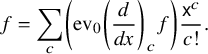
We demonstrate here our technique on a simpler toy example, where we recover the family of normalized monomials ![]() using only the indirect information that they are homogeneous with
using only the indirect information that they are homogeneous with $S_\varnothing =1$
and satisfy
$S_\varnothing =1$
and satisfy
 $$ \begin{align} \frac{d}{dx_i}S_c=\begin{cases}S_{c-e_i}&\text{if }c_i\ge 1\\0&\text{otherwise.}\end{cases} \end{align} $$
where $c-e_i=(c_1,\ldots ,c_{i-1},c_i-1,c_{i+1},\ldots ,c_\ell )$
. Our technique is motivated by Euler’s famous theorem
$c-e_i=(c_1,\ldots ,c_{i-1},c_i-1,c_{i+1},\ldots ,c_\ell )$
. Our technique is motivated by Euler’s famous theorem
 $$ \begin{align*}\sum_{i=1}^\infty x_i\frac{d}{dx_i}f=kf\end{align*} $$
for f a homogeneous polynomial of positive degree k. Iteratively applying this identity shows that
 $$ \begin{align*}\sum_{i_1,\ldots,i_k}x_{i_1}\cdots x_{i_k}\frac{d}{dx_{i_1}}\cdots \frac{d}{dx_{i_k}}f=k!\operatorname{id}\end{align*} $$
on homogeneous polynomials of degree k, and grouping together terms with the same derivatives applied to f shows that
 $$ \begin{align*}\sum_{(c_1,\dots,c_\ell)}\frac{\mathsf{x}^c}{c!}\left(\frac{d}{dx_1}\right)^{c_1}\cdots \left(\frac{d}{dx_k}\right)^{c_\ell}=\mathrm{id}.\end{align*} $$
Applying this identity to $S_c$
shows that
$S_c$
shows that $S_c=\frac {\mathsf {x}^c}{c!}$
, as desired. Notably, this calculation does not use the Ansatz that the family of polynomials we are seeking are monomials.
$S_c=\frac {\mathsf {x}^c}{c!}$
, as desired. Notably, this calculation does not use the Ansatz that the family of polynomials we are seeking are monomials.
Let ![]() , and let
, and let $\operatorname {Pol}^+\subset \operatorname {Pol}$
denote the ideal of polynomials with no constant term. Our method relies on finding degree
$\operatorname {Pol}^+\subset \operatorname {Pol}$
denote the ideal of polynomials with no constant term. Our method relies on finding degree $1$
‘creation operators’
$1$
‘creation operators’ $Y_1,Y_2,\ldots $
that solve the equation
$Y_1,Y_2,\ldots $
that solve the equation
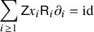
 $$ \begin{align*}\sum_{i=1}^{\infty} Y_i\partial_i=\operatorname{id}\end{align*} $$
on $\operatorname {Pol}^+$
. Applying this equation to a Schubert polynomial and recursing gives an expansion
$\operatorname {Pol}^+$
. Applying this equation to a Schubert polynomial and recursing gives an expansion
 $$ \begin{align*}\sum_{(i_1,\ldots,i_k)\in \operatorname{Red}(w)}Y_{i_k}\cdots Y_{i_1}(1)=\mathfrak{S}_{w},\end{align*} $$
where $\operatorname {Red}(w)$
is the set of reduced words for w. In particular, if each
$\operatorname {Red}(w)$
is the set of reduced words for w. In particular, if each $Y_i$
is a monomial nonnegative operator, then this produces a monomial nonnegative expansion of
$Y_i$
is a monomial nonnegative operator, then this produces a monomial nonnegative expansion of $\mathfrak {S}_{w}$
. Given the simplicity, we now show that Schubert polynomials have a nonnegative monomial expansion using this technique by producing one such family of creation operators (this later appears as §3.1; we will produce an additional family in §5.3). Define the map
$\mathfrak {S}_{w}$
. Given the simplicity, we now show that Schubert polynomials have a nonnegative monomial expansion using this technique by producing one such family of creation operators (this later appears as §3.1; we will produce an additional family in §5.3). Define the map
 $$ \begin{align*}\mathsf{R}_{i}(f)=f(x_1,\ldots,x_{i-1},0,x_i,x_{i+1},\ldots).\end{align*} $$
Then
 $$\begin{align*}\operatorname{id}=\mathsf{R}_{1}+(\mathsf{R}_{2}-\mathsf{R}_{1})+(\mathsf{R}_{3}-\mathsf{R}_{2})+\cdots=\mathsf{R}_{1}+\sum_{i=1}^{\infty}x_i\mathsf{R}_{i}\partial_i. \end{align*}$$
Here, we use $\mathsf {R}_{i+1}-\mathsf {R}_{i}=x_i\mathsf {R}_{i}\partial _{i}$
, which can be seen to hold by noting that
$\mathsf {R}_{i+1}-\mathsf {R}_{i}=x_i\mathsf {R}_{i}\partial _{i}$
, which can be seen to hold by noting that $\mathsf {R}_{i+1}=\mathsf {R}_{i}s_i$
, where
$\mathsf {R}_{i+1}=\mathsf {R}_{i}s_i$
, where $s_i$
is the simple transposition swapping
$s_i$
is the simple transposition swapping $x_i$
and
$x_i$
and $x_{i+1}$
. Moving
$x_{i+1}$
. Moving $\mathsf {R}_{1}$
to the other side and noting that
$\mathsf {R}_{1}$
to the other side and noting that $\mathrm {id}-\mathsf {R}_{1}$
is invertible on polynomials with no constant term with inverse
$\mathrm {id}-\mathsf {R}_{1}$
is invertible on polynomials with no constant term with inverse $\mathsf {Z}=\operatorname {id}+\mathsf {R}_{1}+\mathsf {R}_{1}^2+\cdots $
, we conclude that
$\mathsf {Z}=\operatorname {id}+\mathsf {R}_{1}+\mathsf {R}_{1}^2+\cdots $
, we conclude that
 $$ \begin{align*}\sum \mathsf{Z} x_i\mathsf{R}_{i}\partial_i=\mathrm{id}.\end{align*} $$
Applying this to $\mathfrak {S}_{w}$
immediately gives the following.
$\mathfrak {S}_{w}$
immediately gives the following.
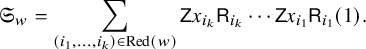
Theorem 1.1 (Corollary 3.2).
We have the following monomial positive expansion:
 $$ \begin{align*}\mathfrak{S}_{w}=\sum_{(i_1,\ldots,i_k)\in \operatorname{Red}(w)}\mathsf{Z} x_{i_k}\mathsf{R}_{i_k}\cdots \mathsf{Z} x_{i_1}\mathsf{R}_{i_1}(1).\end{align*} $$
Example 3.3 demonstrates how this theorem build Schubert polynomials bottom-up.
We generalize these ideas to a more general situation $(X,M)$
we call a ‘divided difference pair’ (dd-pair henceforth), in which the compositions of degree
$(X,M)$
we call a ‘divided difference pair’ (dd-pair henceforth), in which the compositions of degree $-1$
polynomial endomorphisms
$-1$
polynomial endomorphisms $X_1,X_2,\ldots $
, given by ‘shifts’ of a fixed endomorphism X, form a representation of a right-cancellable partial graded monoid M generated in degree
$X_1,X_2,\ldots $
, given by ‘shifts’ of a fixed endomorphism X, form a representation of a right-cancellable partial graded monoid M generated in degree $1$
. Writing
$1$
. Writing $\operatorname {Last}(w)$
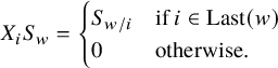
for the analogue of the descent set of w, we will say that a family of polynomials
$\operatorname {Last}(w)$
for the analogue of the descent set of w, we will say that a family of polynomials $\{S_w\;|\; w\in M\}$
is ‘dual’ to the dd-pair if it satisfies the normalization condition
$\{S_w\;|\; w\in M\}$
is ‘dual’ to the dd-pair if it satisfies the normalization condition $S_1=1$
and
$S_1=1$
and
 $$ \begin{align*}X_iS_w=\begin{cases}S_{w/i}&\text{ if }i\in \operatorname{Last}(w)\\0&\text{otherwise.}\end{cases}\end{align*} $$
It is then natural to ask the following.
-
1. Assuming there is such a family of polynomials $\{S_w\;|\; w\in M\}$
, can we write down a formula for
$S_w$
?
$\{S_w\;|\; w\in M\}$
, can we write down a formula for
$S_w$
? -
2. Does such a family of polynomials exist in the first place?


These questions came up naturally from our previous paper [Reference Nadeau, Spink and Tewari22] for the operators
called ‘m-quasisymmetric divided difference operators’. There we had to essentially guess (via computer assistance) a formula for the family of m-forest polynomials and then through a tedious and unenlightening computation [Reference Nadeau, Spink and Tewari22, Appendix] show that they interact in the expected way with the ![]() operators.
operators.
The analogue of creation operators $Y_i$
such that
$Y_i$
such that $\sum Y_iX_i=\operatorname {id}$
on polynomials with no constant term can be used to solve the first question analogously as for Schubert polynomials, and we find such operators for m-forest polynomials without difficulty.
$\sum Y_iX_i=\operatorname {id}$
on polynomials with no constant term can be used to solve the first question analogously as for Schubert polynomials, and we find such operators for m-forest polynomials without difficulty.
For the second question, we show that if a dd-pair has creation operators, then surprisingly, the only additional thing that is needed to ensure that the dual family of polynomials exists is a ‘code map’ $c:M\to \mathsf {Codes}$
from the partial monoid to finitely supported sequences of nonnegative integers, so that the highest index of a nonzero element of
$c:M\to \mathsf {Codes}$
from the partial monoid to finitely supported sequences of nonnegative integers, so that the highest index of a nonzero element of $c(m)$
is the maximal element of
$c(m)$
is the maximal element of $\operatorname {Last}(w)$
. The Lehmer code of permutations works for the
$\operatorname {Last}(w)$
. The Lehmer code of permutations works for the $\partial _i$
formalism, while the m-Dyck path forest code [Reference Nadeau, Spink and Tewari22, Definition 3.5] works for the
$\partial _i$
formalism, while the m-Dyck path forest code [Reference Nadeau, Spink and Tewari22, Definition 3.5] works for the ![]() formalism: this shows directly that Schubert polynomials and m-forest polynomials exist without any Ansatz or combinatorial model.
formalism: this shows directly that Schubert polynomials and m-forest polynomials exist without any Ansatz or combinatorial model.
As a further application, we study the well-known family of polynomials called ‘slide polynomials’ investigated in detail by Assaf–Searles [Reference Assaf and Searles3]; this family is also present in earlier works [Reference Billey, Jockusch and Stanley6, Reference Hivert11] (see [Reference Hicks and Niese10] for more on the relation to Hivert’s foundational work). Forest polynomials and Schubert polynomials decompose nonnegatively in terms of this family (see respectively [Reference Nadeau and Tewari23] and [Reference Assaf and Searles3, Reference Billey, Jockusch and Stanley6]). A slide polynomial is determined by a sequence of positive integers $(a_1,a_2,\ldots ,a_k)$
, and the distinct slide polynomials
$(a_1,a_2,\ldots ,a_k)$
, and the distinct slide polynomials ![]() are indexed by weakly increasing sequences
are indexed by weakly increasing sequences $1\leq a_1\le a_{2}\le \cdots \le a_k$
. We construct a dd-pair for the operators
$1\leq a_1\le a_{2}\le \cdots \le a_k$
. We construct a dd-pair for the operators
whose compositions are governed by the partial monoid whose only relations are that ![]() is undefined for
is undefined for $i>j$
, such that the slide polynomials form the dual family of polynomials. This gives a fast and practical method for directly extracting coefficients of an arbitrary polynomial in the slide basis. Since fundamental quasisymmetric polynomials are a subfamily within slide polynomials, this generalizes [Reference Nadeau, Spink and Tewari22, Corollary 8.6].
$i>j$
, such that the slide polynomials form the dual family of polynomials. This gives a fast and practical method for directly extracting coefficients of an arbitrary polynomial in the slide basis. Since fundamental quasisymmetric polynomials are a subfamily within slide polynomials, this generalizes [Reference Nadeau, Spink and Tewari22, Corollary 8.6].
Theorem 1.2 (Corollary 5.8).
The slide expansion of a degree k homogeneous polynomial $f\in \operatorname {Pol}$
is given by
$f\in \operatorname {Pol}$
is given by
Associated to the ![]() are a new family of operators we call ‘slide creators’
are a new family of operators we call ‘slide creators’ ![]() that have the property that for any sequence
that have the property that for any sequence $a_1,\ldots ,a_k$
(not necessarily weakly increasing), we have
$a_1,\ldots ,a_k$
(not necessarily weakly increasing), we have
and
on $\operatorname {Pol}^+$
, i.e., they function as creation operators for Schubert polynomials, forest polynomials, and slide polynomials themselves simultaneously. Using these facts, we obtain the known slide polynomial expansions of Schubert and forest polynomials.
$\operatorname {Pol}^+$
, i.e., they function as creation operators for Schubert polynomials, forest polynomials, and slide polynomials themselves simultaneously. Using these facts, we obtain the known slide polynomial expansions of Schubert and forest polynomials.
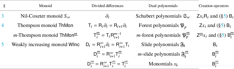
1.1 Outline of the paper
See Table 1 for an overview of where we address each family of polynomials we consider in the paper. In §2, we set up the notion of divided difference pairs and study creation operators and code maps. In §3, we study Schubert polynomials. In §4, we study forest polynomials, including m-forest polynomials. In §5, we study slide polynomials and m-slide polynomials, which include monomials as a limiting case.
Table 1 Divided difference formalisms.
2 Divided differences and creation operators
We describe a general framework which encodes the duality between $\partial _i$
and
$\partial _i$
and $\mathfrak {S}_{w}$
. In our framework, the pair
$\mathfrak {S}_{w}$
. In our framework, the pair $(\partial ,S_{\infty })$
will be called a divided difference pair (dd-pair for short), and
$(\partial ,S_{\infty })$
will be called a divided difference pair (dd-pair for short), and $\{\mathfrak {S}_{w}\;|\; w\in S_{\infty }\}$
will be called a ‘dual family of polynomials’ to this dd-pair. The two main mathematical insights are as follows.
$\{\mathfrak {S}_{w}\;|\; w\in S_{\infty }\}$
will be called a ‘dual family of polynomials’ to this dd-pair. The two main mathematical insights are as follows.
-
1. The existence of certain ‘creation operators’ leads to explicit formulas for the dual polynomials, assuming the dual family of polynomials exist.
-
2. Creation operators together with a ‘code map’ show that the dual polynomials exist, without needing to verify any particular Ansatz or combinatorial model that interacts well with the operators.
These considerations are new and interesting even in the case of Schubert polynomials. For example, because we have the $\mathsf {Z} x\mathsf {R}_{}$
creation operators mentioned in the introduction, we will see in §3 that the existence of the Lehmer code on permutations immediately implies that Schubert polynomials exist without any Ansatz or direct verification that the
$\mathsf {Z} x\mathsf {R}_{}$
creation operators mentioned in the introduction, we will see in §3 that the existence of the Lehmer code on permutations immediately implies that Schubert polynomials exist without any Ansatz or direct verification that the $\mathsf {Z} x\mathsf {R}_{}$
recursion interacts well with the
$\mathsf {Z} x\mathsf {R}_{}$
recursion interacts well with the $\partial _i$
operators. In later sections, we will apply this formalism to other families of polynomials.
$\partial _i$
operators. In later sections, we will apply this formalism to other families of polynomials.
Remark 2.1. The operators and families of polynomials of interest to us in this paper have integer coefficients, so we will set everything up over $\mathbb Z$
. This will exclude certain parts of the
$\mathbb Z$
. This will exclude certain parts of the $\frac {d}{dx_i}$
example from the introduction because of the denominators present in the normalized monomials
$\frac {d}{dx_i}$
example from the introduction because of the denominators present in the normalized monomials $S_c=\frac {\mathsf {x}^c}{c!}$
. However, all of the theorems we have work equally well over
$S_c=\frac {\mathsf {x}^c}{c!}$
. However, all of the theorems we have work equally well over $\mathbb Q$
, and we will indicate through this section how such modifications apply to this particular example.
$\mathbb Q$
, and we will indicate through this section how such modifications apply to this particular example.
2.1 Partial monoids and polynomial representations
We start by recalling some notions on partial monoids: these will encode the combinatorics of relations between families of operators.
A partial monoid M is a set equipped with a partial product map $M\times M \dashrightarrow M$
denoted by concatenation, together with a unit
$M\times M \dashrightarrow M$
denoted by concatenation, together with a unit $1$
, such that
$1$
, such that $1m=m1=m$
for all
$1m=m1=m$
for all $m\in M$
, and
$m\in M$
, and $m(m'm")=(mm')m"$
for any
$m(m'm")=(mm')m"$
for any $m,m',m"$
, in the sense that either both products are undefined, or both are defined and equal.
$m,m',m"$
, in the sense that either both products are undefined, or both are defined and equal.
Remark 2.2. We have a monoid when the map is total – that is, when products are always defined. Given a partial monoid M, one forms a monoid on the one-element extension $M\sqcup \{\mathbf {0}\}$
by setting
$M\sqcup \{\mathbf {0}\}$
by setting $mm'=\mathbf {0}$
when the product is undefined in M, and if m or
$mm'=\mathbf {0}$
when the product is undefined in M, and if m or $m'$
is
$m'$
is $\mathbf {0}$
. The notions of partial monoids and monoids with zero are thus essentially equivalent.
$\mathbf {0}$
. The notions of partial monoids and monoids with zero are thus essentially equivalent.
A polynomial representation of M is a map $\Phi :M\to \operatorname {End}(\operatorname {Pol})$
assigning an endomorphism of
$\Phi :M\to \operatorname {End}(\operatorname {Pol})$
assigning an endomorphism of $\operatorname {Pol}$
to each element of M such that
$\operatorname {Pol}$
to each element of M such that $\Phi (1)=\operatorname {id}$
and such that for
$\Phi (1)=\operatorname {id}$
and such that for $u,v\in M$
, we have
$u,v\in M$
, we have
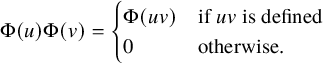 $$ \begin{align*}\Phi(u)\Phi(v)=\begin{cases}\Phi(uv)&\text{if }uv\text{ is defined}\\0&\text{otherwise.}\end{cases}\end{align*} $$
A partial monoid M is graded if there is a length function $\ell :M\to \{0,1,2,\ldots \}$
such that
$\ell :M\to \{0,1,2,\ldots \}$
such that $\ell (uv)=\ell (u)+\ell (v)$
whenever
$\ell (uv)=\ell (u)+\ell (v)$
whenever $uv$
is defined. We write
$uv$
is defined. We write $M_k\subset M$
for those elements of degree k. We always have
$M_k\subset M$
for those elements of degree k. We always have $M_0=\{1\}$
, and we write
$M_0=\{1\}$
, and we write $M_1=\{a_i\}_{i\in I}$
for some indexing set I. If a graded partial monoid is generated in degree
$M_1=\{a_i\}_{i\in I}$
for some indexing set I. If a graded partial monoid is generated in degree $1$
, then the length
$1$
, then the length $\ell (w)$
for
$\ell (w)$
for $w\in M$
is the common length k of all expressions
$w\in M$
is the common length k of all expressions $m=a_{i_1}\cdots a_{i_k}$
. For such a partial monoid, we write
$m=a_{i_1}\cdots a_{i_k}$
. For such a partial monoid, we write $\operatorname {Fac}(w)$
for the set of
$\operatorname {Fac}(w)$
for the set of $(i_1,\ldots ,i_k)$
such that
$(i_1,\ldots ,i_k)$
such that $w=a_{i_1}\cdots a_{i_k}$
, and for
$w=a_{i_1}\cdots a_{i_k}$
, and for $w\in M_k$
, we write
$w\in M_k$
, we write $\operatorname {Last}(w)$
for the set of i such that
$\operatorname {Last}(w)$
for the set of i such that $w=w'a_i$
for some
$w=w'a_i$
for some $w'\in M_{k-1}$
. If such a
$w'\in M_{k-1}$
. If such a $w'$
is always unique, then we say furthermore that M is right-cancellative, and we denote this element by
$w'$
is always unique, then we say furthermore that M is right-cancellative, and we denote this element by $w/i$
. Finally, we say that such an M has finite factorizations if we always have
$w/i$
. Finally, we say that such an M has finite factorizations if we always have $|\operatorname {Fac}(w)|<\infty $
(or equivalently if we always have
$|\operatorname {Fac}(w)|<\infty $
(or equivalently if we always have $|\operatorname {Last}(w)|<\infty $
).
$|\operatorname {Last}(w)|<\infty $
).
2.2 Divided difference pairs
We now formalize the relationship between the divided difference operators $\partial _i$
and the partial monoid
$\partial _i$
and the partial monoid $S_{\infty }$
in what we call a ‘divided difference pair’ (dd-pair). It is not our goal to give the most general results possible but to have a formalism that encompasses all examples we want to treat while being possibly useful in other situations.
$S_{\infty }$
in what we call a ‘divided difference pair’ (dd-pair). It is not our goal to give the most general results possible but to have a formalism that encompasses all examples we want to treat while being possibly useful in other situations.
We fix a polynomial endomorphism $X\in \operatorname {End}(\operatorname {Pol})$
that is of degree
$X\in \operatorname {End}(\operatorname {Pol})$
that is of degree $-1$
(i.e., X takes degree d homogeneous polynomials to degree
$-1$
(i.e., X takes degree d homogeneous polynomials to degree $d-1$
homogeneous polynomials for all d).
$d-1$
homogeneous polynomials for all d).
For any $i\geq 1$
, we define the shifted operator
$i\geq 1$
, we define the shifted operator $X_i\in \operatorname {End}(\operatorname {Pol})$
by the composition
$X_i\in \operatorname {End}(\operatorname {Pol})$
by the composition
 $$ \begin{align*}X_i:\operatorname{Pol}\cong \operatorname{Pol}_{i-1}\otimes \operatorname{Pol} \to \operatorname{Pol}_{i-1}\otimes \operatorname{Pol} \cong \operatorname{Pol},\end{align*} $$
where the first and last isomorphisms are given by the isomorphism
 $$ \begin{align*}\operatorname{Pol}_{i-1}\otimes \operatorname{Pol}=\mathbb Z[x_1,\ldots,x_{i-1}]\otimes \mathbb Z[x_i,x_{i+1},\ldots]\cong \operatorname{Pol},\end{align*} $$
and the middle map is given by $\operatorname {id}\otimes X$
. In particular,
$\operatorname {id}\otimes X$
. In particular, $X=X_1$
and we always have
$X=X_1$
and we always have
 $$ \begin{align} f\in \operatorname{Pol}_n\implies X_{n+1}f=X_{n+2}f=\cdots=0, \end{align} $$
since in this case, X acts on constants and thus vanishes as it has degree $-1$
.
$-1$
.
Example 2.3. If we set $\partial \in \operatorname {End}(\operatorname {Pol})$
to be the first divided difference
$\partial \in \operatorname {End}(\operatorname {Pol})$
to be the first divided difference
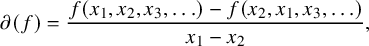 $$ \begin{align} \partial(f)=\frac{f(x_1,x_2,x_3,\ldots)-f(x_2,x_1,x_3,\ldots)}{x_1-x_2},\end{align} $$
then $\partial _i$
agrees with (1.2).
$\partial _i$
agrees with (1.2).
Note that $\partial $
is called the divided difference operator because the formula involves dividing a difference by a linear form. The way in which the various X we consider in later sections arise will also be from taking two degree
$\partial $
is called the divided difference operator because the formula involves dividing a difference by a linear form. The way in which the various X we consider in later sections arise will also be from taking two degree $0$
operators
$0$
operators $A,B\in \operatorname {End}(\operatorname {Pol})$
such that
$A,B\in \operatorname {End}(\operatorname {Pol})$
such that $(A-B)f$
is always divisible by a linear form L, and then setting
$(A-B)f$
is always divisible by a linear form L, and then setting $X=\frac {A-B}{L}$
.
$X=\frac {A-B}{L}$
.
Writing dd for divided difference, we call X and the $X_i$
dd-operators even if they do not necessarily arise in this way in general.
$X_i$
dd-operators even if they do not necessarily arise in this way in general.
Definition 2.4. We define a divided difference pair (or a dd-pair) to be the data of $(X,M)$
, where M is a graded right-cancellative partial monoid, generated in degree
$(X,M)$
, where M is a graded right-cancellative partial monoid, generated in degree $1$
by
$1$
by $\{a_i\}_{i\geq 1}$
, such that the map
$\{a_i\}_{i\geq 1}$
, such that the map $a_i\mapsto X_i$
is a representation of M. For
$a_i\mapsto X_i$
is a representation of M. For $w\in M$
, we write
$w\in M$
, we write $X_w$
for the associated endomorphism of
$X_w$
for the associated endomorphism of $\operatorname {Pol}$
, and in particular, we have
$\operatorname {Pol}$
, and in particular, we have $X_i=X_{a_i}$
.
$X_i=X_{a_i}$
.
Example 2.5. If we set $M=S_{\infty }$
with its partial monoid structure given by (1.1),
$M=S_{\infty }$
with its partial monoid structure given by (1.1), $\partial $
as in (2.2), then the divided difference representation
$\partial $
as in (2.2), then the divided difference representation $s_i\mapsto \partial _i$
makes
$s_i\mapsto \partial _i$
makes $(\partial ,S_{\infty })$
into a dd-pair.
$(\partial ,S_{\infty })$
into a dd-pair.
Example 2.6. For any degree $-1$
polynomial endomorphism X, we have
$-1$
polynomial endomorphism X, we have $(X,M)$
is a dd-pair for M the free monoid on
$(X,M)$
is a dd-pair for M the free monoid on $\{1,2,\ldots \}$
.
$\{1,2,\ldots \}$
.
Example 2.7. $\mathsf {Codes}$
is a monoid via componentwise addition, and we have a representation given by
$\mathsf {Codes}$
is a monoid via componentwise addition, and we have a representation given by $i\mapsto \frac {d}{dx_i}$
because
$i\mapsto \frac {d}{dx_i}$
because $\frac {d}{dx_i}\frac {d}{dx_j}=\frac {d}{dx_j}\frac {d}{dx_i}$
. Therefore,
$\frac {d}{dx_i}\frac {d}{dx_j}=\frac {d}{dx_j}\frac {d}{dx_i}$
. Therefore, $(\frac {d}{dx},\mathsf {Codes})$
is a dd-pair, and for
$(\frac {d}{dx},\mathsf {Codes})$
is a dd-pair, and for $c=(c_1,\dots ,c_k,0,\ldots )$
, we have
$c=(c_1,\dots ,c_k,0,\ldots )$
, we have $\left (\frac {d}{dx}\right )_c=\left (\frac {d}{dx_1}\right )^{c_1}\cdots \left (\frac {d}{dx_k}\right )^{c_k}$
.
$\left (\frac {d}{dx}\right )_c=\left (\frac {d}{dx_1}\right )^{c_1}\cdots \left (\frac {d}{dx_k}\right )^{c_k}$
.
We are especially interested in the case where M encodes all additive relations between compositions of the operators $X_i$
. However, this is a hard thing to show in general, so we do not want to assume it from the beginning. It will actually follow from the formalism we now introduce (see Theorem 2.20).
$X_i$
. However, this is a hard thing to show in general, so we do not want to assume it from the beginning. It will actually follow from the formalism we now introduce (see Theorem 2.20).
2.3 Dual families of polynomials to a dd-pair
We now generalize the relation between $\mathfrak {S}_{w}$
and the
$\mathfrak {S}_{w}$
and the $\partial _i$
to an arbitrary dd-pair
$\partial _i$
to an arbitrary dd-pair $(X,M)$
.
$(X,M)$
.
Definition 2.8. A family $(S_w)_{w\in M}$
of homogeneous polynomials in
$(S_w)_{w\in M}$
of homogeneous polynomials in $\operatorname {Pol}$
is dual to a dd-pair
$\operatorname {Pol}$
is dual to a dd-pair $(X,M)$
if
$(X,M)$
if $S_{1}=1$
, and for each
$S_{1}=1$
, and for each $w\in M$
and
$w\in M$
and $i\in \{1,2,\ldots \}$
, we have
$i\in \{1,2,\ldots \}$
, we have
 $$\begin{align*}X_iS_w=\begin{cases}S_{w/i}&\text{if }i\in \operatorname{Last}(w)\\0&\text{otherwise.}\end{cases} \end{align*}$$
Example 2.9. The Schubert polynomials $\{\mathfrak {S}_{w}\;|\; w\in S_{\infty }\}$
are dual to the dd-pair
$\{\mathfrak {S}_{w}\;|\; w\in S_{\infty }\}$
are dual to the dd-pair $(\partial ,S_{\infty })$
.
$(\partial ,S_{\infty })$
.
Example 2.10. If we had defined everything over $\mathbb Q$
instead of
$\mathbb Q$
instead of $\mathbb Z$
, then
$\mathbb Z$
, then $\{\frac {\mathsf {x}^c}{c!}\;|\; c\in \mathsf {Codes}\}$
would be dual to to the dd-pair
$\{\frac {\mathsf {x}^c}{c!}\;|\; c\in \mathsf {Codes}\}$
would be dual to to the dd-pair $(\frac {d}{dx},\mathsf {Codes})$
.
$(\frac {d}{dx},\mathsf {Codes})$
.
The terminology is justified by item (4) of the following result.
Proposition 2.11. If a dd-pair $(X,M)$
has a dual family
$(X,M)$
has a dual family $\{S_w\;|\; w\in M\}$
, then
$\{S_w\;|\; w\in M\}$
, then
-
(1) M has finite factorizations.
-
(2) The polynomials
$S_w$
are
$\mathbb Z$
-linearly independent. -
(3) The representation of
$\mathbb Z[M]$
is faithful: In particular, M is the partial monoid of compositions generated by the operators
$$ \begin{align*}\sum c_wX_w=0\implies c_w=0\text{ for all }w.\end{align*} $$
$X_i$
.
-
(4) Letting
$\operatorname {ev}_{0}:\operatorname {Pol}\to \mathbb Z$
be the map
$f\mapsto f(0,0,\dots )$
, we have
$\operatorname {ev}_{0} X_vS_{w}=\delta _{v,w}$
. As a consequence, for
$f\in \mathbb Z\{S_w\;|\; w\in M\}$
, the
$\mathbb Z$
-span of the
$S_w$
, we have (2.3)
$$ \begin{align} f=\sum_{w\in M}(\operatorname{ev}_{0} X_w f)S_w.\end{align} $$


Proof. First, note that for $(i_1,\ldots ,i_k)\in \operatorname {Fac}(w)$
, we have
$(i_1,\ldots ,i_k)\in \operatorname {Fac}(w)$
, we have $X_{i_1}\cdots X_{i_k}S_w=S_1=1$
. Now we know that for any polynomial f, there are only finitely many
$X_{i_1}\cdots X_{i_k}S_w=S_1=1$
. Now we know that for any polynomial f, there are only finitely many $X_i$
such that
$X_i$
such that $X_if\ne 0$
. Applying this repeatedly, we see there are only finitely many sequences
$X_if\ne 0$
. Applying this repeatedly, we see there are only finitely many sequences $(i_1,\ldots ,i_k)$
such that
$(i_1,\ldots ,i_k)$
such that $X_{i_1}\cdots X_{i_k}S_w\ne 0$
. Therefore,
$X_{i_1}\cdots X_{i_k}S_w\ne 0$
. Therefore, $|\operatorname {Fac}(w)|<\infty $
, and (1) is proved.
$|\operatorname {Fac}(w)|<\infty $
, and (1) is proved.
The defining relations for $S_w$
imply that
$S_w$
imply that $X_vS_w=S_u$
if there exists a
$X_vS_w=S_u$
if there exists a $u\in M$
(necessarily unique by right-cancellability) such that
$u\in M$
(necessarily unique by right-cancellability) such that $w=vu$
, and
$w=vu$
, and $0$
otherwise. Since
$0$
otherwise. Since $S_u$
is homogeneous of degree
$S_u$
is homogeneous of degree $\ell (u)$
, we have
$\ell (u)$
, we have $\operatorname {ev}_{0} S_u=\delta _{1,u}$
, so
$\operatorname {ev}_{0} S_u=\delta _{1,u}$
, so $\operatorname {ev}_{0} X_vS_w=\delta _{v,w}$
, establishing the first part of (4). This implies that the linear functionals
$\operatorname {ev}_{0} X_vS_w=\delta _{v,w}$
, establishing the first part of (4). This implies that the linear functionals $\{\operatorname {ev}_{0} X_v\;|\; v\in M\}$
are dual to the family of polynomials
$\{\operatorname {ev}_{0} X_v\;|\; v\in M\}$
are dual to the family of polynomials $\{S_w\;|\; w\in M\}$
, so the polynomials
$\{S_w\;|\; w\in M\}$
, so the polynomials $\{S_w\;|\; w\in M\}$
are linearly independent and the linear functionals
$\{S_w\;|\; w\in M\}$
are linearly independent and the linear functionals $\{\operatorname {ev}_{0} X_w\;|\; w\in M\}$
are linearly independent, establishing (2) and (3). Finally, for f in the
$\{\operatorname {ev}_{0} X_w\;|\; w\in M\}$
are linearly independent, establishing (2) and (3). Finally, for f in the $\mathbb Z$
-span of the
$\mathbb Z$
-span of the $S_w$
, if we write
$S_w$
, if we write $f=\sum b_vS_v$
, then applying
$f=\sum b_vS_v$
, then applying $\operatorname {ev}_{0} X_w$
to both sides shows
$\operatorname {ev}_{0} X_w$
to both sides shows $b_w=\operatorname {ev}_{0} X_w f$
which implies the reconstruction formula (2.3).
$b_w=\operatorname {ev}_{0} X_w f$
which implies the reconstruction formula (2.3).
Example 2.12. We give an example of a dd-pair whose dual family does not span $\operatorname {Pol}$
. Let
$\operatorname {Pol}$
. Let $\partial '=\partial _2$
. For the dd-pair
$\partial '=\partial _2$
. For the dd-pair $(\partial ',S_{\infty })$
where
$(\partial ',S_{\infty })$
where $s_i\mapsto (\partial ')_i=\partial _{i+1}$
, for each
$s_i\mapsto (\partial ')_i=\partial _{i+1}$
, for each $\lambda \in \mathbb Z$
, we can construct a dual family of polynomials
$\lambda \in \mathbb Z$
, we can construct a dual family of polynomials $S_{w}^{(\lambda )}=\mathfrak {S}_{w}(\lambda x_1+x_2,\lambda x_1+x_3,\ldots )$
. For no
$S_{w}^{(\lambda )}=\mathfrak {S}_{w}(\lambda x_1+x_2,\lambda x_1+x_3,\ldots )$
. For no $\lambda $
does this family of polynomials span
$\lambda $
does this family of polynomials span $\operatorname {Pol}$
since
$\operatorname {Pol}$
since $x_1$
is not in the span of the linear polynomials.
$x_1$
is not in the span of the linear polynomials.
Example 2.13. The analogue of Proposition 2.11 still holds if we had used $\mathbb Q$
instead of
$\mathbb Q$
instead of $\mathbb Z$
in our setup. In this case, the existence of the dual family of monomials
$\mathbb Z$
in our setup. In this case, the existence of the dual family of monomials $\frac {\mathsf {x}^c}{c!}$
to the dd-pair
$\frac {\mathsf {x}^c}{c!}$
to the dd-pair $(\frac {d}{dx},\mathsf {Codes})$
shows that the representation of
$(\frac {d}{dx},\mathsf {Codes})$
shows that the representation of $\mathsf {Codes}$
is faithful, and (2.3) recovers the Taylor expansion of any rational polynomial f:
$\mathsf {Codes}$
is faithful, and (2.3) recovers the Taylor expansion of any rational polynomial f:
 $$ \begin{align*}f=\sum_c \left(\operatorname{ev}_{0} \left(\frac{d}{dx}\right)_c f\right)\frac{\mathsf{x}^c}{c!}.\end{align*} $$
2.4 Creation operators and code maps
Given a dd-pair, an outstanding remaining question is whether they do admit a dual family of polynomials $S_w$
. We give an answer in several cases of interest, using the existence of certain ‘creation operators’.
$S_w$
. We give an answer in several cases of interest, using the existence of certain ‘creation operators’.
Definition 2.14. We define creation operators for the operator X to be a collection of degree $1$
polynomial endomorphisms
$1$
polynomial endomorphisms $Y_i\in \operatorname {End}(\operatorname {Pol})$
such that on the ideal
$Y_i\in \operatorname {End}(\operatorname {Pol})$
such that on the ideal $\operatorname {Pol}^+\subset \operatorname {Pol}$
, we have the identity
$\operatorname {Pol}^+\subset \operatorname {Pol}$
, we have the identity
 $$ \begin{align} \sum_{i=1}^{\infty} Y_iX_i=\mathrm{id}. \end{align} $$
We will further say that a dd-pair $(X,M)$
has creation operators when the operator X does.
$(X,M)$
has creation operators when the operator X does.
Note that the left-hand side of (2.4) is well defined thanks to (2.1).
Remark 2.15. Note that the left-hand side of (2.4) vanishes on $\mathbb Z$
, so the identity extends uniquely to
$\mathbb Z$
, so the identity extends uniquely to $\operatorname {Pol}$
by subtracting
$\operatorname {Pol}$
by subtracting $\operatorname {ev}_{0}$
from the right-hand side (i.e., it reads
$\operatorname {ev}_{0}$
from the right-hand side (i.e., it reads $\sum _{i=1}^{\infty } Y_iX_i=\operatorname {id}-\operatorname {ev}_{0}).$
Proposition 2.16. If a dd-pair $(X,M)$
has creation operators
$(X,M)$
has creation operators $Y_i$
and a family of dual polynomials
$Y_i$
and a family of dual polynomials $\{S_w\;|\; w\in M\}$
, then for
$\{S_w\;|\; w\in M\}$
, then for $w\in M$
, we have
$w\in M$
, we have
 $$ \begin{align} S_w=\sum_{(i_1,\dots,i_k)\in \operatorname{Fac}(w)} Y_{i_k}\cdots Y_{i_1}(1). \end{align} $$
Proof.
M has finite factorizations by Proposition 2.11, so the right-hand side in (2.5) is well defined. To prove it, we induct on the length $k=\ell (w)$
. For
$k=\ell (w)$
. For $k=0$
, this is the identity
$k=0$
, this is the identity $S_{1}=1$
, and for
$S_{1}=1$
, and for $k>0$
, we have
$k>0$
, we have
 $$ \begin{align*} S_w= \sum_{i=1}^{\infty}Y_iX_iS_w=\sum_{i\in \operatorname{Last}(w)}Y_iS_{w/i} &=\sum_{i\in \operatorname{Last}(w)}\sum_{(i_1,\dots,i_{k-1})\in \operatorname{Fac}(w/i)}Y_iY_{i_{k-1}}\cdots Y_{i_1}(1) \nonumber\\ &=\sum_{(i_1,\dots,i_k)\in \operatorname{Fac}(w)}Y_{i_k}\cdots Y_{i_1}(1).\\[-47pt] \end{align*} $$
An immediate consequence is that if a dd-pair has creation operators, it has at most one dual family of polynomials. The creation operators are not unique in general, and this leads to possibly distinct expansions of $S_w$
as we will see in later sections.
$S_w$
as we will see in later sections.
Example 2.17. If we had used $\mathbb Q$
instead of
$\mathbb Q$
instead of $\mathbb Z$
in our setup, then for
$\mathbb Z$
in our setup, then for $(\frac {d}{dx},\mathsf {Codes})$
, we can take
$(\frac {d}{dx},\mathsf {Codes})$
, we can take $Y_i$
to act on homogeneous polynomials of degree k by
$Y_i$
to act on homogeneous polynomials of degree k by $Y_i(f)=\frac {1}{k+1}x_if$
for all k. Then (2.4) holds as it is Euler’s famous theorem
$Y_i(f)=\frac {1}{k+1}x_if$
for all k. Then (2.4) holds as it is Euler’s famous theorem $\sum x_i\frac {d}{dx_i}=k\operatorname {id}$
on homogeneous polynomials of positive degree k. For
$\sum x_i\frac {d}{dx_i}=k\operatorname {id}$
on homogeneous polynomials of positive degree k. For $c=(c_i)_{i\geq 1}\in \mathsf {Codes}$
, we have
$c=(c_i)_{i\geq 1}\in \mathsf {Codes}$
, we have $\operatorname {Fac}(c)=\{(i_1,\ldots ,i_k)\;|\; c_p=\#\{1\leq j\leq k\;|\; i_j=p\}\}$
, and (2.5) recovers the formula
$\operatorname {Fac}(c)=\{(i_1,\ldots ,i_k)\;|\; c_p=\#\{1\leq j\leq k\;|\; i_j=p\}\}$
, and (2.5) recovers the formula $S_c=\frac {\mathsf {x}^c}{c!}$
for the unique candidate family of polynomials satisfying (1.3).
$S_c=\frac {\mathsf {x}^c}{c!}$
for the unique candidate family of polynomials satisfying (1.3).
Let us give an example now to show that the existence of creation operators is not enough to ensure the existence of a dual family of polynomials.
Example 2.18. Define X by linearly extending the assignments $X(x_i)=\delta _{i,1}$
for all
$X(x_i)=\delta _{i,1}$
for all $i\ge 1$
, and some degree
$i\ge 1$
, and some degree $-1$
injection
$-1$
injection $\Phi $
on monomials of degree d to monomials of degree
$\Phi $
on monomials of degree d to monomials of degree $d-1$
for each
$d-1$
for each $d\ge 2$
. We can assume that
$d\ge 2$
. We can assume that $x_1$
does not occur in the range of
$x_1$
does not occur in the range of $\Phi $
, by applying the shift
$\Phi $
, by applying the shift $x_i\mapsto x_{i+1}$
if necessary. X has the following creation operators
$x_i\mapsto x_{i+1}$
if necessary. X has the following creation operators $Y_i$
: on the constant polynomials,
$Y_i$
: on the constant polynomials, $Y_i$
is multiplication by
$Y_i$
is multiplication by $x_i$
. On
$x_i$
. On $\operatorname {Pol}^+$
, define
$\operatorname {Pol}^+$
, define $Y_2=Y_3=\cdots =0$
while
$Y_2=Y_3=\cdots =0$
while $Y_1$
equals
$Y_1$
equals $\Phi ^{-1}$
on monomials in the range of
$\Phi ^{-1}$
on monomials in the range of $\Phi $
, and
$\Phi $
, and $0$
on the remaining monomials.
$0$
on the remaining monomials.
If $(S_w)_{w\in M}$
is dual to some dd-pair
$(S_w)_{w\in M}$
is dual to some dd-pair $(X,M)$
, we have
$(X,M)$
, we have $S_{a_1}=x_1$
. Now
$S_{a_1}=x_1$
. Now $a_1\cdot a_1$
is defined in M since
$a_1\cdot a_1$
is defined in M since $X_1^2=X^2$
is nonzero, and we have
$X_1^2=X^2$
is nonzero, and we have $X_1(S_{a_1\cdot a_1})=x_1$
. This is not possible by our assumption on
$X_1(S_{a_1\cdot a_1})=x_1$
. This is not possible by our assumption on $\Phi $
, and thus,
$\Phi $
, and thus, $(X,M)$
does not have a dual family.
$(X,M)$
does not have a dual family.
We now give an easily checkable hypothesis on M that ensures that the dual polynomials do in fact exist and, furthermore, form a basis of $\operatorname {Pol}$
.
$\operatorname {Pol}$
.
Let $\mathsf {Codes}$
denote the set of finitely supported sequences of nonnegative integers
$\mathsf {Codes}$
denote the set of finitely supported sequences of nonnegative integers $c=(c_1,c_2,\ldots )$
. For
$c=(c_1,c_2,\ldots )$
. For $c\in \mathsf {Codes}$
, write
$c\in \mathsf {Codes}$
, write $\operatorname {supp} c$
for the set of i such that
$\operatorname {supp} c$
for the set of i such that $c_i\neq 0$
, and
$c_i\neq 0$
, and $|c|$
for the sum of the nonzero entries. Let M be a graded right cancellable monoid.
$|c|$
for the sum of the nonzero entries. Let M be a graded right cancellable monoid.
Definition 2.19. A code map for M is an injective map $c:M\to \mathsf {Codes}$
such that
$c:M\to \mathsf {Codes}$
such that $\ell (w)=|c(w)|$
and
$\ell (w)=|c(w)|$
and $\max \operatorname {supp} c(w)=\max \operatorname {Last}(w)$
for all
$\max \operatorname {supp} c(w)=\max \operatorname {Last}(w)$
for all $w\in M$
. (In particular, M has finite factorizations.)
$w\in M$
. (In particular, M has finite factorizations.)
We note that the existence of a code map is trivially seen to be equivalent to the condition that
 $$ \begin{align*}\#\{w\in M\;|\; \ell(w)=n\text{ and }\max \operatorname{Last}(w)=k\}\le \#\{c\in \mathsf{Codes}\;|\; |c(w)|=n\text{ and }\max\operatorname{supp} c(w)=k\},\end{align*} $$
but in practice, verifying code maps exist seems to be more straightforward than checking this inequality by other means.
Theorem 2.20. Suppose that a dd-pair $(X,M)$
has creation operators and a code map. Then
$(X,M)$
has creation operators and a code map. Then
-
(1) The code map is bijective.
-
(2) There is a unique dual family
$(S_w)_{w\in M}$
defined by (2.5). It is a basis of
$\operatorname {Pol}$
. -
(3) The subfamily
$(S_w)_w$
where
$\max \operatorname {supp} c(w)\le d$
is a basis of
$\operatorname {Pol}_d$
for any
$d\geq 0$
.


Proof. Define recursively $S_1=1$
and
$S_1=1$
and
 $$\begin{align*}S_w=\sum_{i\in \operatorname{Last}(w)}Y_iS_{w/i}. \end{align*}$$
By Proposition 2.16, the dual family of polynomials must be equal to $\{S_w\;|\; w\in M\}$
if it exists.
$\{S_w\;|\; w\in M\}$
if it exists.
We begin by addressing (1). Let
 $$ \begin{align*}M_{k,d}=\{w\in M\;|\; \ell(w)=k\text{ and }\max\operatorname{supp} c(w)\le d\}.\end{align*} $$
We claim that for $f\in \operatorname {Pol}_d^{(k)}$
, the homogeneous degree k polynomials in
$f\in \operatorname {Pol}_d^{(k)}$
, the homogeneous degree k polynomials in $\operatorname {Pol}_d$
, we have
$\operatorname {Pol}_d$
, we have
 $$ \begin{align} f=\sum_{w\in M_{k,d}}X_w(f)S_w. \end{align} $$
By induction on k, we can show (2.6) but with $w\in M_{k,d}$
replaced with the condition
$w\in M_{k,d}$
replaced with the condition $\ell (w)=k$
since
$\ell (w)=k$
since
 $$ \begin{align*}f=\sum_{i=1}^{\infty} Y_iX_if=\sum_{i=1}^{\infty}Y_i\sum_{\ell(w')=k-1}(X_{w'}X_if)S_{w'}=\sum_{\ell(w)=k}\sum_{i\in \operatorname{Last}(w)}Y_i(X_w(f)S_{w/i})=\sum_{\ell(w)=k}X_w(f)S_w.\end{align*} $$
To conclude, it suffices to show that if $\ell (w)=k$
and
$\ell (w)=k$
and $w\not \in M_{k,d}$
, then
$w\not \in M_{k,d}$
, then $X_wf=0$
; this is true because if
$X_wf=0$
; this is true because if $i=\max \operatorname {supp} c(w)>d$
, then
$i=\max \operatorname {supp} c(w)>d$
, then $i\in \operatorname {Last}(w)$
and so
$i\in \operatorname {Last}(w)$
and so $X_wf=X_{w/i}X_if=0.$
Writing $\mathsf {Codes}_{k,d}=\{c\in \mathsf {Codes} \;|\; \max \operatorname {supp} c\le d\text { and }|c(w)|=k\}$
, the code map induces an injection
$\mathsf {Codes}_{k,d}=\{c\in \mathsf {Codes} \;|\; \max \operatorname {supp} c\le d\text { and }|c(w)|=k\}$
, the code map induces an injection $M_{k,d}\to \mathsf {Codes}_{k,d}$
so
$M_{k,d}\to \mathsf {Codes}_{k,d}$
so $|M_{k,d}|\le |\mathsf {Codes}_{k,d}|$
. However, (2.6) implies the inclusion
$|M_{k,d}|\le |\mathsf {Codes}_{k,d}|$
. However, (2.6) implies the inclusion
 $$ \begin{align}\operatorname{Pol}_d^{(k)}\subset \mathbb Z\{S_w\;|\; w\in M_{k,d}\},\end{align} $$
so $|\mathsf {Codes}_{k,d}|=\operatorname {rank} \operatorname {Pol}_d^{(k)}\le |M_{k,d}|$
. We conclude that
$|\mathsf {Codes}_{k,d}|=\operatorname {rank} \operatorname {Pol}_d^{(k)}\le |M_{k,d}|$
. We conclude that $|M_{k,d}|=|\mathsf {Codes}_{k,d}|=\operatorname {rank} \operatorname {Pol}_d^{(k)}$
, implying (1) and the fact the
$|M_{k,d}|=|\mathsf {Codes}_{k,d}|=\operatorname {rank} \operatorname {Pol}_d^{(k)}$
, implying (1) and the fact the $S_w$
are
$S_w$
are $\mathbb Z$
-linearly independent.
$\mathbb Z$
-linearly independent.
Observe that (2.7) is a containment of equal rank free abelian groups. Furthermore, $\operatorname {Pol}_d^{(k)}$
is saturated (i.e., for any
$\operatorname {Pol}_d^{(k)}$
is saturated (i.e., for any $\lambda \in \mathbb Z$
, we have
$\lambda \in \mathbb Z$
, we have $\lambda f\in \operatorname {Pol}_d^{(k)}$
implies
$\lambda f\in \operatorname {Pol}_d^{(k)}$
implies $f\in \operatorname {Pol}_d^{(k)}$
), so the containment (2.7) is in fact an equality, and we conclude that
$f\in \operatorname {Pol}_d^{(k)}$
), so the containment (2.7) is in fact an equality, and we conclude that $\{S_w\;|\; w\in M_{k,d}\}$
is a
$\{S_w\;|\; w\in M_{k,d}\}$
is a $\mathbb Z$
-basis of
$\mathbb Z$
-basis of $\operatorname {Pol}_d^{(k)}$
. Taking the union of these bases for all k and fixed d shows that
$\operatorname {Pol}_d^{(k)}$
. Taking the union of these bases for all k and fixed d shows that $\{S_w\;|\; \max \operatorname {supp} c(w)\le d\}$
is a basis for
$\{S_w\;|\; \max \operatorname {supp} c(w)\le d\}$
is a basis for $\operatorname {Pol}_d$
, which shows (3).
$\operatorname {Pol}_d$
, which shows (3).
By considering these basis statements and the identity (2.6) for growing d, and using the fact that $\bigcup M_{k,d}=M$
, we deduce that
$\bigcup M_{k,d}=M$
, we deduce that $\{S_w\;|\; w\in M\}$
is a basis of
$\{S_w\;|\; w\in M\}$
is a basis of $\operatorname {Pol}$
, proving the second half of (2). For arbitrary
$\operatorname {Pol}$
, proving the second half of (2). For arbitrary $f\in \operatorname {Pol}$
, we have the identity
$f\in \operatorname {Pol}$
, we have the identity
 $$ \begin{align*}f=\sum_{w\in M}(\operatorname{ev}_{0} X_wf)S_w.\end{align*} $$
We thus infer that
-
(a) If
$\operatorname {ev}_{0} X_wf=0$
for all
$w\in M$
, then
$f=0$
, and -
(b)
$S_w$
is the unique polynomial such that
$\operatorname {ev}_{0} X_{w'}S_w=\delta _{w',w}$
for all
$w'\in M$
.


We are now ready to show that $X_iS_w=\delta _{i\in \operatorname {Last}(w)}S_{w/i}$
for any i and w.Footnote
1
If
$X_iS_w=\delta _{i\in \operatorname {Last}(w)}S_{w/i}$
for any i and w.Footnote
1
If $w'\in M$
, we have
$w'\in M$
, we have
 $$ \begin{align*}\operatorname{ev}_{0} X_{w'}(X_iS_w)=\operatorname{ev}_{0} X_{w'\cdot i}S_w=\delta_{w,w'\cdot i}.\end{align*} $$
Here, the last two terms are considered as zero if $w'\cdot i$
is not defined. If
$w'\cdot i$
is not defined. If $i\not \in \operatorname {Last}(w)$
, then
$i\not \in \operatorname {Last}(w)$
, then $\delta _{w,w'\cdot i}=0$
for all
$\delta _{w,w'\cdot i}=0$
for all $w'\in M$
, so we conclude by (a) that
$w'\in M$
, so we conclude by (a) that $X_iS_w=0$
. However, if
$X_iS_w=0$
. However, if $i\in \operatorname {Last}(w)$
, then
$i\in \operatorname {Last}(w)$
, then $\delta _{w,w'\cdot i}=\delta _{w/i,w'}$
, which by (b) implies
$\delta _{w,w'\cdot i}=\delta _{w/i,w'}$
, which by (b) implies $X_iS_w=S_{w/i}$
, as desired.
$X_iS_w=S_{w/i}$
, as desired.
Example 2.21. For $(\frac {d}{dx},\mathsf {Codes})$
, there is a code map on
$(\frac {d}{dx},\mathsf {Codes})$
, there is a code map on $\mathsf {Codes}$
given by the identity. Therefore, using
$\mathsf {Codes}$
given by the identity. Therefore, using $\mathbb Q$
instead of
$\mathbb Q$
instead of $\mathbb Z$
in our setup, we can conclude that
$\mathbb Z$
in our setup, we can conclude that $\{S_c=\frac {\mathsf {x}^c}{c!}\;|\; c\in \mathsf {Codes}\}$
found in Example 2.17 is the dual family of polynomials to
$\{S_c=\frac {\mathsf {x}^c}{c!}\;|\; c\in \mathsf {Codes}\}$
found in Example 2.17 is the dual family of polynomials to $(\frac {d}{dx},\mathsf {Codes})$
without directly verifying the recursion (1.3).
$(\frac {d}{dx},\mathsf {Codes})$
without directly verifying the recursion (1.3).
3 Schubert polynomials
The divided difference $\partial _i\in \operatorname {End}(\operatorname {Pol})$
for
$\partial _i\in \operatorname {End}(\operatorname {Pol})$
for $i=1,2,\dots $
is defined as follows:
$i=1,2,\dots $
is defined as follows:
 $$ \begin{align*} \partial_if(x_1,x_2,\ldots)&=\frac{f-f(x_1,\dots,x_{i-1},x_{i+1},x_{i},\ldots)}{x_i-x_{i+1}}. \end{align*} $$
The partial monoid M is given by the nil-Coxeter monoid $S_{\infty }$
of permutations of
$S_{\infty }$
of permutations of $\{1,2,\ldots \}$
fixing all but finitely many elements with partial product
$\{1,2,\ldots \}$
fixing all but finitely many elements with partial product $u\circ v=uv$
if
$u\circ v=uv$
if $\ell (u)+\ell (v)=\ell (uv)$
, undefined otherwise: here,
$\ell (u)+\ell (v)=\ell (uv)$
, undefined otherwise: here, $\ell $
and
$\ell $
and $uv$
are the lengths and product in the group
$uv$
are the lengths and product in the group $S_{\infty }$
. Denoting the simple transposition
$S_{\infty }$
. Denoting the simple transposition $s_i=(i,i+1)$
, the corresponding dd-pair
$s_i=(i,i+1)$
, the corresponding dd-pair $(\partial ,S_{\infty })$
comes from the representation
$(\partial ,S_{\infty })$
comes from the representation $s_i\mapsto \partial _i$
.
$s_i\mapsto \partial _i$
.
We have
 $$ \begin{align*}\operatorname{Last}(w)=\operatorname{Des}(w)=\{i\;|\; w(i)>w(i+1)\},\end{align*} $$
and $\operatorname {Fac}(w)=\operatorname {Red}(w)$
, the set of reduced words for w (i.e., the set of sequences
$\operatorname {Fac}(w)=\operatorname {Red}(w)$
, the set of reduced words for w (i.e., the set of sequences $(i_1,\ldots ,i_k)$
with
$(i_1,\ldots ,i_k)$
with $k=\ell (w)$
such that
$k=\ell (w)$
such that $w=s_{i_1}\cdots s_{i_k}$
). The Lehmer code is the bijective map
$w=s_{i_1}\cdots s_{i_k}$
). The Lehmer code is the bijective map $S_{\infty }\to \mathsf {Codes}$
defined for
$S_{\infty }\to \mathsf {Codes}$
defined for $w\in S_{\infty }$
by
$w\in S_{\infty }$
by $\operatorname {lcode}(w)=(c_1,c_2,\ldots )$
, where
$\operatorname {lcode}(w)=(c_1,c_2,\ldots )$
, where $c_i=\#\{j>i\;|\; w(i)>w(j)\}$
. Because
$c_i=\#\{j>i\;|\; w(i)>w(j)\}$
. Because $\operatorname {Des}(w)=\{i\;|\; c_i>c_{i+1}\}$
, we have
$\operatorname {Des}(w)=\{i\;|\; c_i>c_{i+1}\}$
, we have $\max \operatorname {supp} \operatorname {lcode}(w)=\max \operatorname {Last}(w)$
, so this is a code map as in Definition 2.19.
$\max \operatorname {supp} \operatorname {lcode}(w)=\max \operatorname {Last}(w)$
, so this is a code map as in Definition 2.19.
The Schubert polynomials are the unique family of homogeneous polynomials dual to the dd-pair $(\partial , S_{\infty })$
: we have
$(\partial , S_{\infty })$
: we have $\mathfrak {S}_{\operatorname {id}}=1$
and
$\mathfrak {S}_{\operatorname {id}}=1$
and
 $$ \begin{align*}\partial_i\mathfrak{S}_{w}=\begin{cases}\mathfrak{S}_{w/i}& \text{if }i\in \operatorname{Des}(w)\\0&\text{otherwise.}\end{cases}\end{align*} $$
Figure 1 shows the application of various divided difference operators starting from $\mathfrak {S}_{1432}$
.
$\mathfrak {S}_{1432}$
.
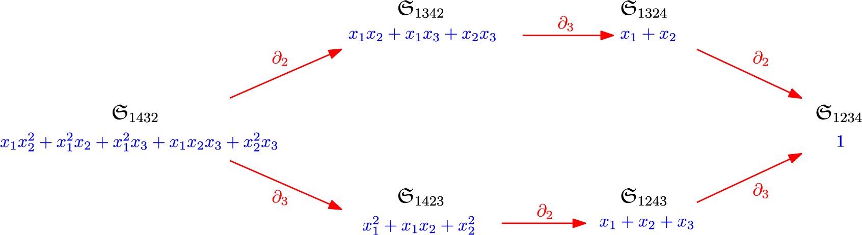
Figure 1 Sequences of $\partial _i$
applied to a
$\partial _i$
applied to a $\mathfrak {S}_{w}$
.
$\mathfrak {S}_{w}$
.
The standard way the existence of Schubert polynomials is shown is through the Ansatz $\mathfrak {S}_{w_{0,n}}=x_1^{n-1}x_2^{n-2}\cdots x_{n-1}$
for
$\mathfrak {S}_{w_{0,n}}=x_1^{n-1}x_2^{n-2}\cdots x_{n-1}$
for $w_{0,n}$
the longest permutation in
$w_{0,n}$
the longest permutation in $S_n$
. Because every
$S_n$
. Because every $u\in S_{\infty }$
has
$u\in S_{\infty }$
has $u\le w_{0,n}$
for some n, it turns out it suffices to check that
$u\le w_{0,n}$
for some n, it turns out it suffices to check that $\partial _{w_{0,n-1}^{-1}w_{0,n}}x_1^{n-1}x_2^{n-2}\cdots x_{n-1}=x_1^{n-2}x_2^{n-3}\cdots x_{n-2}$
, which is done with direct calculation.
$\partial _{w_{0,n-1}^{-1}w_{0,n}}x_1^{n-1}x_2^{n-2}\cdots x_{n-1}=x_1^{n-2}x_2^{n-3}\cdots x_{n-2}$
, which is done with direct calculation.
Using our setup, because there is a code map, we can simultaneously avoid the Ansatz and establish an explicit combinatorial formula by exhibiting creation operators for the $\partial _i$
.
$\partial _i$
.
3.1 Creation operators for
$\partial _i$

We now describe creation operators for $\partial _i$
, which will give formulas for the Schubert polynomials. We define the Bergeron–Sottile map [Reference Bergeron and Sottile5]
$\partial _i$
, which will give formulas for the Schubert polynomials. We define the Bergeron–Sottile map [Reference Bergeron and Sottile5]
 $$ \begin{align*}\mathsf{R}_{i}f(x_1,x_2,\ldots)=f(x_1,\ldots,x_{i-1},0,x_i,\ldots).\end{align*} $$
Lemma 3.1. We have
 $$ \begin{align*} \sum_{i\geq 1} x_i\mathsf{R}_{i}\partial_i= \operatorname{id}-\mathsf{R}_{1}. \end{align*} $$
Proof. We sum the relation $x_i\mathsf {R}_{i}\partial _i=\mathsf {R}_{i+1}-\mathsf {R}_{i}$
for all
$x_i\mathsf {R}_{i}\partial _i=\mathsf {R}_{i+1}-\mathsf {R}_{i}$
for all $i\geq 1$
.
$i\geq 1$
.
We define
 $$ \begin{align*}\mathsf{Z}=\operatorname{id}+\mathsf{R}_{1}+\mathsf{R}_{1}^2+\cdots:\operatorname{Pol}^+\to \operatorname{Pol}^+.\end{align*} $$
Corollary 3.2. We have that $\mathsf {Z} x_i\mathsf {R}_{i}$
are creation operators for the dd-pair given by the usual divided differences
$\mathsf {Z} x_i\mathsf {R}_{i}$
are creation operators for the dd-pair given by the usual divided differences $\partial _i$
and the nil-Coxeter monoid. That is, the identity
$\partial _i$
and the nil-Coxeter monoid. That is, the identity
 $$ \begin{align*}\sum_{i\ge 1}\mathsf{Z} x_i\mathsf{R}_{i}\partial_i=\operatorname{id}\end{align*} $$
holds on $\operatorname {Pol}^+$
. In particular, Schubert polynomials exist, and we have the following monomial positive expansion:
$\operatorname {Pol}^+$
. In particular, Schubert polynomials exist, and we have the following monomial positive expansion:
 $$ \begin{align*}\mathfrak{S}_{w}=\sum_{(i_1,\ldots,i_k)\in \operatorname{Red}(w)}\mathsf{Z} x_{i_k}\mathsf{R}_{i_k}\cdots \mathsf{Z} x_{i_1}\mathsf{R}_{i_1}(1).\end{align*} $$
Proof. We compute $\mathsf {Z}\sum _{i\geq 1} x_i\mathsf {R}_{i}\partial _i=Z(\operatorname {id}-\mathsf {R}_{1})=(\operatorname {id}-\mathsf {R}_{1})+\mathsf {R}_{1}(\operatorname {id}-\mathsf {R}_{1})+\cdots =\operatorname {id}$
.
$\mathsf {Z}\sum _{i\geq 1} x_i\mathsf {R}_{i}\partial _i=Z(\operatorname {id}-\mathsf {R}_{1})=(\operatorname {id}-\mathsf {R}_{1})+\mathsf {R}_{1}(\operatorname {id}-\mathsf {R}_{1})+\cdots =\operatorname {id}$
.
Example 3.3. Take $w=14253$
so that
$w=14253$
so that $\operatorname {Red}(w)=\{324,342\}$
. Adopting the shorthand
$\operatorname {Red}(w)=\{324,342\}$
. Adopting the shorthand $\mathsf {Z} \textsf {x}\mathsf {R}_{\mathbf {i}}$
for composite
$\mathsf {Z} \textsf {x}\mathsf {R}_{\mathbf {i}}$
for composite $\mathsf {Z} x_{i_k}\mathsf {R}_{i_k}\cdots \mathsf {Z} x_{i_1}\mathsf {R}_{i_1}$
where
$\mathsf {Z} x_{i_k}\mathsf {R}_{i_k}\cdots \mathsf {Z} x_{i_1}\mathsf {R}_{i_1}$
where $\mathbf {i}=(i_1,\dots ,i_k)$
, one gets
$\mathbf {i}=(i_1,\dots ,i_k)$
, one gets
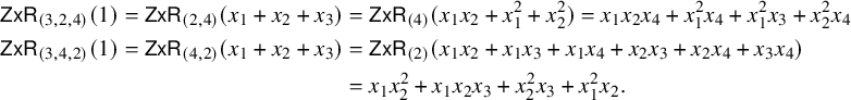 $$ \begin{align*} \mathsf{Z}\textsf{x}\mathsf{R}_{(3,2,4)}(1)= \mathsf{Z}\textsf{x}\mathsf{R}_{(2,4)}(x_1+x_2+x_3)&= \mathsf{Z}\textsf{x}\mathsf{R}_{(4)}(x_1x_2+x_1^2+x_2^2)=x_1x_2x_4+x_1^2x_4+x_1^2x_3+x_2^2x_4 \\\mathsf{Z}\textsf{x}\mathsf{R}_{(3,4,2)}(1)= \mathsf{Z}\textsf{x}\mathsf{R}_{(4,2)}(x_1+x_2+x_3)&= \mathsf{Z}\textsf{x}\mathsf{R}_{(2)}(x_1x_2+x_1x_3+x_1x_4+x_2x_3+x_2x_4+x_3x_4)\\&=x_1x_2^2+x_1x_2x_3+x_2^2x_3+x_1^2x_2. \end{align*} $$
On adding the two right-hand sides, one obtains the Schubert polynomial $\mathfrak {S}_{14253}$
.
$\mathfrak {S}_{14253}$
.
Remark 3.4. The slide expansion of Schubert polynomials [Reference Assaf and Searles3, Reference Billey, Jockusch and Stanley6], reproved in Proposition 5.7, expresses $\mathfrak {S}_{w}$
as a sum of slide polynomials over
$\mathfrak {S}_{w}$
as a sum of slide polynomials over $\operatorname {Red}(w)$
. Corollary 3.2 also provides an expression where the sum ranges over
$\operatorname {Red}(w)$
. Corollary 3.2 also provides an expression where the sum ranges over $\operatorname {Red}(w)$
, but these two decompositions are in fact distinct, as the preceding example reveals as neither
$\operatorname {Red}(w)$
, but these two decompositions are in fact distinct, as the preceding example reveals as neither $\mathsf {Z}\textsf {x}\mathsf {R}_{(3,2,4)}(1)$
nor
$\mathsf {Z}\textsf {x}\mathsf {R}_{(3,2,4)}(1)$
nor $\mathsf {Z}\textsf {x}\mathsf {R}_{(3,4,2)}(1)$
equals a slide polynomial.
$\mathsf {Z}\textsf {x}\mathsf {R}_{(3,4,2)}(1)$
equals a slide polynomial.
3.2 Pipe dream interpretation
We now relate the preceding results to a simple bijection at the level of pipe dreams. Consider the staircase ![]() whose columns are labeled
whose columns are labeled $1$
through n left to right. Given
$1$
through n left to right. Given $w\in S_n$
, a (reduced) pipe dream for w is a tiling of
$w\in S_n$
, a (reduced) pipe dream for w is a tiling of $\textsf {Stair}_n$
using ‘cross’ and ‘elbow’ tiles depicted in Figure 2 so that the following conditions hold:
$\textsf {Stair}_n$
using ‘cross’ and ‘elbow’ tiles depicted in Figure 2 so that the following conditions hold:
-
• The tilings form n pipes with the pipe entering in row i exiting via column
$w(i)$
for all
$1\leq i\leq n$
; -
• No two pipes intersect more than once.


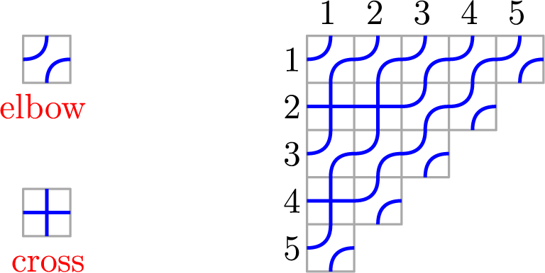
Figure 2 Elbow and cross tiles (left) and a pipe dream for $w=14253$
(right).
$w=14253$
(right).
Denote the set of pipe dreams for w by $\operatorname {PD}(w)$
. Given
$\operatorname {PD}(w)$
. Given $D\in \operatorname {PD}(w)$
, attach the monomial
$D\in \operatorname {PD}(w)$
, attach the monomial
A famous result of Billey–Jockusch–Stanley [Reference Billey, Jockusch and Stanley6] (see also [Reference Bergeron and Billey4, Reference Fomin and Kirillov8, Reference Fomin and Stanley9]) then states that
Theorem 3.5. $\mathfrak {S}_{w}$
is the generating polynomial for pipe dreams for w:
$\mathfrak {S}_{w}$
is the generating polynomial for pipe dreams for w:
 $$\begin{align*}\mathfrak{S}_{w}=\sum_{D\in \operatorname{PD}(w)}\textsf{x}^{D}. \end{align*}$$
We will give a simple proof, using the recursion
 $$ \begin{align} \mathfrak{S}_{w}=\mathsf{R}_{1}\mathfrak{S}_{w}+\sum_{i\in \operatorname{Des}(w)}x_i\mathsf{R}_{i}\mathfrak{S}_{ws_i}, \end{align} $$
which follows immediately from Lemma 3.1 and the definition of Schubert polynomials.
Proof of Theorem 3.5.
We need to show
 $$ \begin{align*}\sum_{D\in \operatorname{PD}(w)}\mathsf{x}^D=\mathsf{R}_{1}\sum_{D\in \operatorname{PD}(w)}\mathsf{x}^D+\sum_{i\in \operatorname{Des}(w)}x_i\mathsf{R}_{i}\sum_{D\in \operatorname{PD}(ws_i)}\mathsf{x}^D.\end{align*} $$
Say that a pipe dream $D\in \operatorname {PD}(w)$
is uncritical if there are no crosses in column
$D\in \operatorname {PD}(w)$
is uncritical if there are no crosses in column $1$
, and i-critical if the last cross in column
$1$
, and i-critical if the last cross in column $1$
is in row i. Denote
$1$
is in row i. Denote $\operatorname {PD}(w)^0\subset \operatorname {PD}(w)$
for the set of uncritical pipe dreams, and
$\operatorname {PD}(w)^0\subset \operatorname {PD}(w)$
for the set of uncritical pipe dreams, and $\operatorname {PD}(w)^i\subset \operatorname {PD}(w)$
for the set of i-critical pipe dreams.
$\operatorname {PD}(w)^i\subset \operatorname {PD}(w)$
for the set of i-critical pipe dreams.
Note that if $i\ge 1$
and
$i\ge 1$
and $\operatorname {PD}(w)^i$
is nonempty, then
$\operatorname {PD}(w)^i$
is nonempty, then $i\in \operatorname {Des}(w)$
since pipes i and
$i\in \operatorname {Des}(w)$
since pipes i and $i+1$
cross at the location of this last cross in column
$i+1$
cross at the location of this last cross in column $1$
. Because
$1$
. Because $\operatorname {PD}(w)=\bigsqcup \operatorname {PD}(w)^i$
, it suffices to show that
$\operatorname {PD}(w)=\bigsqcup \operatorname {PD}(w)^i$
, it suffices to show that
-
(a)
$\sum _{D\in \operatorname {PD}(w)^0 }\mathsf {x}^D=\mathsf {R}_{1}\sum _{D\in \operatorname {PD}(w)}\mathsf {x}^D$
and -
(b) for
$i\in \operatorname {Des}(w)$
we have
$\sum _{D\in \operatorname {PD}(w)^i}\mathsf {x}^D=x_i\mathsf {R}_{i}\sum _{D\in \operatorname {PD}(ws_i)}\mathsf {x}^D$
.


To see (a), we note there is a weight-preserving bijection
 $$ \begin{align*}\Phi_0:\operatorname{PD}(w)^0\to \{D\in \operatorname{PD}(w)\;|\; D\text{ has no crosses in row }1\},\end{align*} $$
given by shifting all crosses one unit diagonally southwest. Since $\mathsf {x}^D=\mathsf {R}_{1}x^{\Phi _0(D)}$
, we have (a).
$\mathsf {x}^D=\mathsf {R}_{1}x^{\Phi _0(D)}$
, we have (a).
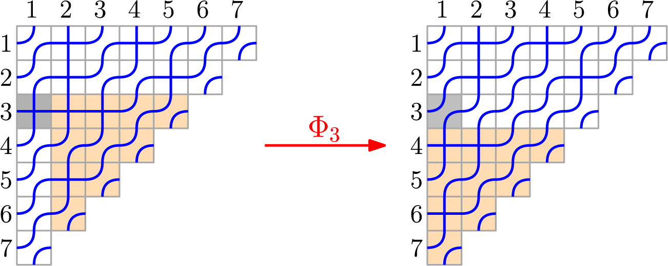
Figure 3 A $3$
-critical pipe dream D for
$3$
-critical pipe dream D for $w=1375264$
(left), and
$w=1375264$
(left), and $\Phi _3(D)\in \operatorname {PD}(ws_3)$
.
$\Phi _3(D)\in \operatorname {PD}(ws_3)$
.
To see (b), we note there is a bijection
 $$ \begin{align*}\Phi_i:\operatorname{PD}(w)^i\to \{D\in \operatorname{PD}(ws_i)\;|\; \text{D has no crosses in row }i\}\end{align*} $$
obtained by turning the last cross in column $1$
into an elbow and then shifting all crosses in rows i and below one unit diagonally southwest. See Figure 3 for an illustration. As
$1$
into an elbow and then shifting all crosses in rows i and below one unit diagonally southwest. See Figure 3 for an illustration. As $\mathsf {x}^{D}=x_i\mathsf {R}_{i}\mathsf {x}^{\Phi _i(D)}$
, we have (b).
$\mathsf {x}^{D}=x_i\mathsf {R}_{i}\mathsf {x}^{\Phi _i(D)}$
, we have (b).
Remark 3.6. Since the image of $\partial _i$
comprises polynomials symmetric in
$\partial _i$
comprises polynomials symmetric in $\{x_i,x_{i+1}\}$
, we can replace the
$\{x_i,x_{i+1}\}$
, we can replace the $\mathsf {R}_{i}\partial _i$
in Lemma 3.1 by
$\mathsf {R}_{i}\partial _i$
in Lemma 3.1 by $\mathsf {R}_{i+1}\partial _i$
. The recursion in (3.1) is then equivalent to
$\mathsf {R}_{i+1}\partial _i$
. The recursion in (3.1) is then equivalent to
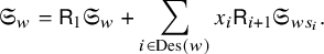 $$ \begin{align} \mathfrak{S}_{w}=\mathsf{R}_{1}\mathfrak{S}_{w}+\sum_{i\in \operatorname{Des}(w)}x_i\mathsf{R}_{i+1}\mathfrak{S}_{ws_i}. \end{align} $$
Dave Anderson has given a representation-theoretic proof [Reference Anderson1] of the recursion in (3.2) using Kraśkiewicz–Pragacz modules [Reference Kraśkiewicz and Pragacz13, Reference Kraśkiewicz and Pragacz14].
4 Forest polynomials
The quasisymmetric divided difference [Reference Nadeau, Spink and Tewari22] is defined as
The associated dd-pair ![]() from [Reference Nadeau, Spink and Tewari22] comes from the monoid structure on the set
from [Reference Nadeau, Spink and Tewari22] comes from the monoid structure on the set ![]() of plane indexed binary forests as we shall briefly recall.
of plane indexed binary forests as we shall briefly recall.
A rooted plane binary tree T is a rooted tree with the property that every node has either no child, in which case we call it a leaf, or two children, distinguished as the ‘left’ and ‘right’ child, in which case we call it an internal node. We let $\operatorname {IN}(T)$
denote the set of internal nodes and let
$\operatorname {IN}(T)$
denote the set of internal nodes and let ![]() be the size of T. The unique tree of size
be the size of T. The unique tree of size $0$
, whose root node is also its leaf node, is denoted by
$0$
, whose root node is also its leaf node, is denoted by $*$
. We shall call this the trivial tree.
$*$
. We shall call this the trivial tree.
An indexed forest F is a sequence $(T_i)_{i\geq 1}$
of rooted plane binary trees where all but finitely many
$(T_i)_{i\geq 1}$
of rooted plane binary trees where all but finitely many $T_i$
are trivial. If all
$T_i$
are trivial. If all $T_i$
are trivial, then we call F the empty forest
$T_i$
are trivial, then we call F the empty forest $\varnothing $
. By identifying the leaves with
$\varnothing $
. By identifying the leaves with $\mathbb Z_{\ge 1}$
, going through them from left to right, one can depict an indexed forest as shown in Figure 4. We denote the set of indexed forests by
$\mathbb Z_{\ge 1}$
, going through them from left to right, one can depict an indexed forest as shown in Figure 4. We denote the set of indexed forests by ![]() . Given
. Given ![]() , we let
, we let ![]() denote its set of internal nodes.
denote its set of internal nodes.
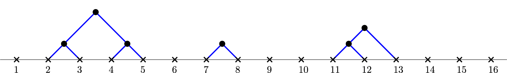
Figure 4 An indexed forest F with $\mathsf {c}(F)=(0,2,0,1,0,0,1,0,0,0,2,0,0,\dots )$
.
$\mathsf {c}(F)=(0,2,0,1,0,0,1,0,0,0,2,0,0,\dots )$
.
There is a natural monoid structure on ![]() obtained by taking
obtained by taking $F\cdot G$
to be the indexed forest where the i’th leaf of F is identified with the i’th root of G for all i. This monoid is generated by the smallest nontrivial forests
$F\cdot G$
to be the indexed forest where the i’th leaf of F is identified with the i’th root of G for all i. This monoid is generated by the smallest nontrivial forests $\underline {i}$
of size
$\underline {i}$
of size $1$
with internal node having left leaf at i, and there is an identification of
$1$
with internal node having left leaf at i, and there is an identification of ![]() with the (right-cancellable) Thompson monoid
with the (right-cancellable) Thompson monoid ![]() given by
given by
by identifying $\underline {i}\mapsto i$
.
$\underline {i}\mapsto i$
.
We may encode ![]() as elements of
as elements of $\mathsf {Codes}$
as follows. Define
$\mathsf {Codes}$
as follows. Define $\rho _F:\operatorname {IN}(F)\to \mathbb Z_{\ge 1}$
by setting
$\rho _F:\operatorname {IN}(F)\to \mathbb Z_{\ge 1}$
by setting $\rho _F(v)$
equal to the label of the leaf obtained by going down left edges from v. Then the map
$\rho _F(v)$
equal to the label of the leaf obtained by going down left edges from v. Then the map ![]() sending
sending $F\mapsto \mathsf {c}(F)=(c_i)_{i\ge 1}$
where
$F\mapsto \mathsf {c}(F)=(c_i)_{i\ge 1}$
where $c_i=\{v\;|\; \rho _F(v)=i\}$
is a bijection [Reference Nadeau, Spink and Tewari22, Theorem 3.6]. The set
$c_i=\{v\;|\; \rho _F(v)=i\}$
is a bijection [Reference Nadeau, Spink and Tewari22, Theorem 3.6]. The set $\operatorname {Last}(w)$
is identified with the left terminal set of F as
$\operatorname {Last}(w)$
is identified with the left terminal set of F as
which in particular immediately implies that $\max \operatorname {supp} c(F)=\max \operatorname {Last}(F)$
, so
$\max \operatorname {supp} c(F)=\max \operatorname {Last}(F)$
, so $\mathsf {c}$
is a code map. We explain the choice of name. We call
$\mathsf {c}$
is a code map. We explain the choice of name. We call $v\in \operatorname {IN}(F)$
terminal if both its children are leaves, necessarily i and
$v\in \operatorname {IN}(F)$
terminal if both its children are leaves, necessarily i and $i+1$
where
$i+1$
where ![]() . We then have
. We then have $c_i\neq 0$
and
$c_i\neq 0$
and $c_{i+1}=0$
(i.e.,
$c_{i+1}=0$
(i.e., ![]() ). Thus, we can record terminal nodes by recording the label of their left leaf, which is what
). Thus, we can record terminal nodes by recording the label of their left leaf, which is what ![]() does.
does.
For ![]() and
and ![]() , we call
, we call ![]() the trimmed forest (as in [Reference Nadeau, Spink and Tewari22, §3.6]), which is obtained by deleting the terminal node v satisfying
the trimmed forest (as in [Reference Nadeau, Spink and Tewari22, §3.6]), which is obtained by deleting the terminal node v satisfying $\rho _F(v)=i$
. The set of factorizations
$\rho _F(v)=i$
. The set of factorizations $\operatorname {Fac}(F)$
is then identified with the set of trimming sequences [Reference Nadeau, Spink and Tewari22, Definition 3.8]:
$\operatorname {Fac}(F)$
is then identified with the set of trimming sequences [Reference Nadeau, Spink and Tewari22, Definition 3.8]:
 $$\begin{align*}\operatorname{Trim}({F})=\{(i_1,\dots,i_k)\;|\; (((F/i_k)/i_{k-1})/\cdots)/i_1 =\varnothing \}. \end{align*}$$
Figure 5 (ignoring the polynomials in blue) shows repeated trimming operators applied to the indexed forest F on the left. It follows that $\operatorname {Trim}({F})=\{(1,1,3),(1,2,1)\}$
.
$\operatorname {Trim}({F})=\{(1,1,3),(1,2,1)\}$
.
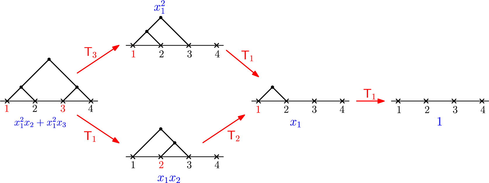
Figure 5
![]() applied to various
applied to various ![]() , with elements of
, with elements of ![]() highlighted in red.
highlighted in red.
4.1 Creation operators for
We now describe creation operators for ![]() .
.
Theorem 4.1. We have ![]() on
on $\operatorname {Pol}^+$
, or in other words,
$\operatorname {Pol}^+$
, or in other words, $\mathsf {Z} x_i$
are creation operators for
$\mathsf {Z} x_i$
are creation operators for ![]() . In particular, there is a family of ‘forest polynomials’
. In particular, there is a family of ‘forest polynomials’ ![]() characterized by
characterized by ![]() and
and
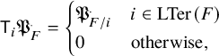
with the following monomial-positive expansion:
Proof. Corollary 3.2 already contains this identity in the form $\sum _{i\geq 1} \mathsf {Z} x_i\mathsf {R}_{i}\partial _i=\operatorname {id}$
on
$\sum _{i\geq 1} \mathsf {Z} x_i\mathsf {R}_{i}\partial _i=\operatorname {id}$
on $\operatorname {Pol}^+$
. The rest follows from Theorem 2.20.
$\operatorname {Pol}^+$
. The rest follows from Theorem 2.20.
Figure 5 shows the result of applying ![]() and
and ![]() to the forest polynomial
to the forest polynomial ![]() . As per Theorem 4.1, each application of a
. As per Theorem 4.1, each application of a ![]() trims the indexed forest at that stage.
trims the indexed forest at that stage.
Example 4.2. We shall consider the indexed forest F whose corresponding forest polynomial ![]() is computed in [Reference Nadeau and Tewari23, Example 3.9]. This happens to be equal to
is computed in [Reference Nadeau and Tewari23, Example 3.9]. This happens to be equal to $\mathfrak {S}_{14253}$
from Example 3.3, but as we shall see, the decompositions are different. We have
$\mathfrak {S}_{14253}$
from Example 3.3, but as we shall see, the decompositions are different. We have $\operatorname {Trim}({F})=\{(2,2,4),(2,3,2)\}$
. Adopting the shorthand
$\operatorname {Trim}({F})=\{(2,2,4),(2,3,2)\}$
. Adopting the shorthand $\mathsf {Z} \textsf {x}_{\mathbf {i}}$
for the composite
$\mathsf {Z} \textsf {x}_{\mathbf {i}}$
for the composite $\mathsf {Z} x_{i_k}\cdots \mathsf {Z} x_{i_1}$
where
$\mathsf {Z} x_{i_k}\cdots \mathsf {Z} x_{i_1}$
where $\mathbf {i}=(i_1,\dots ,i_k)$
, one gets
$\mathbf {i}=(i_1,\dots ,i_k)$
, one gets
 $$ \begin{align*} &\mathsf{Z}\textsf{x}_{(2,2,4)}(1)= \mathsf{Z}\textsf{x}_{(2,4)}(x_1+x_2)= \mathsf{Z}\textsf{x}_{(4)}(x_1x_2+x_1^2+x_2^2)=x_1x_2x_4+x_1^2x_4+x_1^2x_3+x_2^2x_4 \\ &\mathsf{Z}\textsf{x}_{(2,3,2)}(1)= \mathsf{Z}\textsf{x}_{(3,2)}(x_1+x_2)= \mathsf{Z}\textsf{x}_{(2)}(x_1x_2+x_1x_3+x_2x_3)=x_1x_2^2+x_1x_2x_3+x_2^2x_3+x_1^2x_2. \end{align*} $$
Thus, we find that ![]() is the sum of the two right-hand sides. Observe that even though two final expressions above align with those computed in Example 3.3, the expressions obtained at the intermediate stages are not the same.
is the sum of the two right-hand sides. Observe that even though two final expressions above align with those computed in Example 3.3, the expressions obtained at the intermediate stages are not the same.
4.2 Diagrammatic Interpretation
We now give a diagrammatic perspective on forest polynomials that evokes the pipe dream perspective on Schubert polynomials. By applying the relation ![]() from Corollary 3.2 to forest polynomials, we obtain
from Corollary 3.2 to forest polynomials, we obtain
This identity was previously obtained in [Reference Nadeau and Tewari23, Lemma 3.12]. Unwinding this recursion leads to the following combinatorial model similar to the pipe dream expansion of Schubert polynomials, which can be matched up without much difficulty to the combinatorial definitions of forest polynomials in [Reference Nadeau, Spink and Tewari22, Reference Nadeau and Tewari23].
We will represent each of the operators $\mathsf {R}_{1}$
and
$\mathsf {R}_{1}$
and ![]() as a certain graph on a
as a certain graph on a $(\mathbb Z_{\ge 1} \times 2)$
-rectangle as shown in Figure 6 on the left. Consider the grid
$(\mathbb Z_{\ge 1} \times 2)$
-rectangle as shown in Figure 6 on the left. Consider the grid $\mathbb Z_{\ge 1}\times \mathbb Z_{\ge 1}$
where we adopt matrix notation (i.e. the elements in the grid are
$\mathbb Z_{\ge 1}\times \mathbb Z_{\ge 1}$
where we adopt matrix notation (i.e. the elements in the grid are $(i,j)\in \mathbb Z_{\ge 1}\times \mathbb Z_{\ge 1}$
, where the first coordinate increases top to bottom and the second coordinate increases left to right).
$(i,j)\in \mathbb Z_{\ge 1}\times \mathbb Z_{\ge 1}$
, where the first coordinate increases top to bottom and the second coordinate increases left to right).
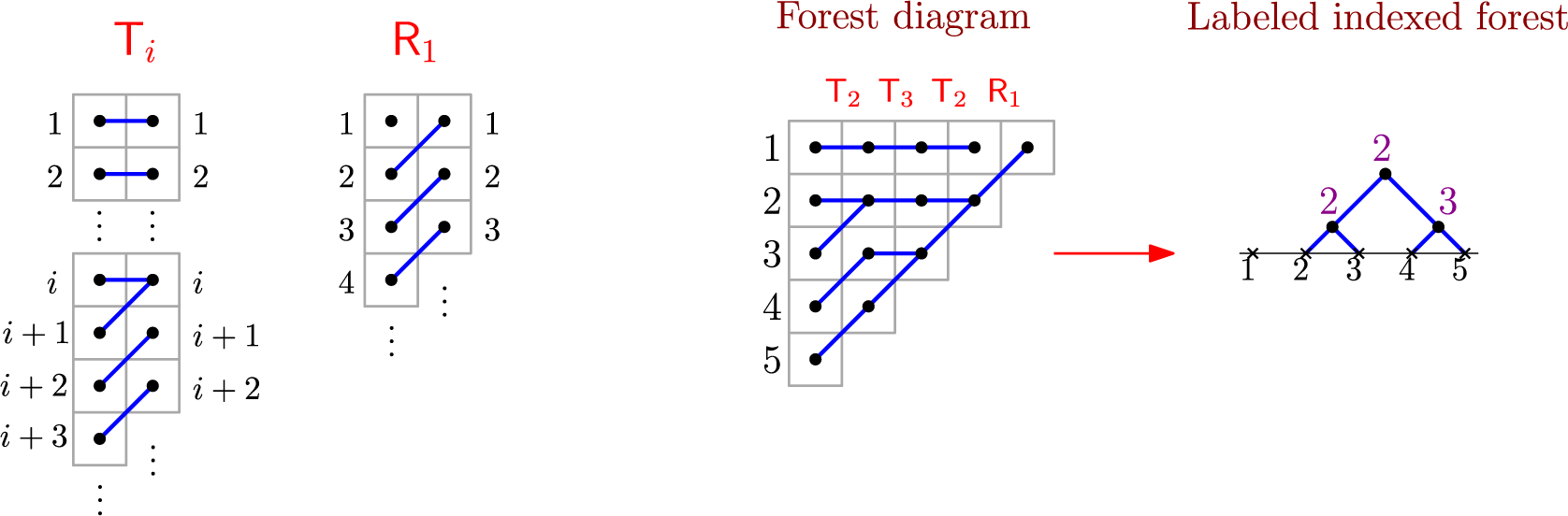
Figure 6 The graphs corresponding to ![]() and
and $\mathsf {R}_{1}$
(left), and a forest diagram with the corresponding labeled indexed forest (right).
$\mathsf {R}_{1}$
(left), and a forest diagram with the corresponding labeled indexed forest (right).
We define a forest diagram to be any graph on vertex set $\mathbb Z_{\ge 1}\times \mathbb Z_{\ge 1}$
such that the subgraph induced on the vertex set
$\mathbb Z_{\ge 1}\times \mathbb Z_{\ge 1}$
such that the subgraph induced on the vertex set $\{(p,q)\;|\; p\in \mathbb Z_{\ge 1}, q\in \{k,k+1\}\}$
either represents
$\{(p,q)\;|\; p\in \mathbb Z_{\ge 1}, q\in \{k,k+1\}\}$
either represents ![]() for some positive integer i or represents
for some positive integer i or represents $\mathsf {R}_{1}$
, and such that for p large enough, all such induced subgraphs represent
$\mathsf {R}_{1}$
, and such that for p large enough, all such induced subgraphs represent $\mathsf {R}_{1}$
. In particular, we may without loss of information restrict our attention to the finite subgraph on the vertex set
$\mathsf {R}_{1}$
. In particular, we may without loss of information restrict our attention to the finite subgraph on the vertex set $\{(i,j)\;|\; i+j\leq n+1\}$
for some n. See on the right in Figure 6 for an example. Given any such diagram D, we let
$\{(i,j)\;|\; i+j\leq n+1\}$
for some n. See on the right in Figure 6 for an example. Given any such diagram D, we let $\textrm {nodes}(D)$
denote the set of
$\textrm {nodes}(D)$
denote the set of $(i,j)$
, where we have
$(i,j)$
, where we have $(i,j)$
directly connected to both
$(i,j)$
directly connected to both $(i,j-1)$
and
$(i,j-1)$
and $(i+1,j-1)$
, and associate a monomial
$(i+1,j-1)$
, and associate a monomial
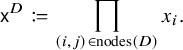
Note that any such graph is necessarily acyclic and naturally corresponds to an indexed forest, as shown in Figure 6. For ![]() , let
, let $\operatorname {Diag}(F)$
denote the set of diagrams whose underlying forest is F.
$\operatorname {Diag}(F)$
denote the set of diagrams whose underlying forest is F.
Theorem 4.3. For ![]() , we have the forest diagram formula
, we have the forest diagram formula
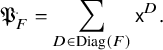
Proof. We give a brisk proof sketch that the claimed expansion satisfies (4.1) along the lines of the proof of Theorem 3.5.
Call $D\in \operatorname {Diag}(F)\ i$
-critical if the subgraph induced on
$D\in \operatorname {Diag}(F)\ i$
-critical if the subgraph induced on $\{(j,1),(j,2)\;|\; j\ge 1\}$
represents
$\{(j,1),(j,2)\;|\; j\ge 1\}$
represents ![]() for some positive integer i. Otherwise, we call D uncritical, in which case the aforementioned subgraph necessarily represents
for some positive integer i. Otherwise, we call D uncritical, in which case the aforementioned subgraph necessarily represents $\mathsf {R}_{1}$
. Note that if D is i-critical, then
$\mathsf {R}_{1}$
. Note that if D is i-critical, then ![]() .
.
Denote by $\operatorname {Diag}(F)^0$
the set of uncritical forest diagrams, and by
$\operatorname {Diag}(F)^0$
the set of uncritical forest diagrams, and by $\operatorname {Diag}(F)^i$
the set of i-critical forest diagrams. Consider the weight-preserving bijection
$\operatorname {Diag}(F)^i$
the set of i-critical forest diagrams. Consider the weight-preserving bijection
 $$\begin{align*}\Phi_0:\operatorname{Diag}(F)^0\to \{D\in \operatorname{Diag}(F)\;|\; \text{no element of nodes(D) is in row }1\} \end{align*}$$
given by shifting all nodes one unit diagonally southwest. Clearly, $\mathsf {x}^D=\mathsf {R}_{1}\mathsf {x}^{\Phi _0(D)}$
.
$\mathsf {x}^D=\mathsf {R}_{1}\mathsf {x}^{\Phi _0(D)}$
.
Consider next the bijection
 $$\begin{align*}\Phi_i:\operatorname{Diag}(F)^i\to \{D\in \operatorname{Diag}(F/i)\} \end{align*}$$
given by taking the subgraph induced on vertices $(p,q)$
with
$(p,q)$
with $p\geq 1, q\geq 2$
. That is, we ignore vertices of the form
$p\geq 1, q\geq 2$
. That is, we ignore vertices of the form $(p,1)$
as well as all incident edges. It is easily seen that
$(p,1)$
as well as all incident edges. It is easily seen that $\mathsf {x}^{D}=x_i\, \mathsf {x}^{\Phi _i(D)}$
.
$\mathsf {x}^{D}=x_i\, \mathsf {x}^{\Phi _i(D)}$
.
4.3 m-forest polynomials
We now briefly touch upon the more general family of m-forest polynomials defined combinatorially in [Reference Nadeau, Spink and Tewari22], where the $m=1$
case recovers the forest polynomials from earlier. By replacing binary forests with
$m=1$
case recovers the forest polynomials from earlier. By replacing binary forests with $(m+1)$
-ary forests, there is an analogously defined set
$(m+1)$
-ary forests, there is an analogously defined set ![]() whose compositional monoid structure is analogously identified with the m-Thompson monoid
whose compositional monoid structure is analogously identified with the m-Thompson monoid
All of the combinatorics and constructions stated specifically for ![]() carry over with minor modifications.
carry over with minor modifications.
In the terminology of the present paper, the m-forest polynomials ![]() are the unique family of polynomials dual to the dd-pair
are the unique family of polynomials dual to the dd-pair ![]() given by m-quasisymmetric divided differences
given by m-quasisymmetric divided differences
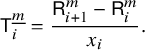
These polynomials were shown to exist in [Reference Nadeau, Spink and Tewari22] by a laborious explicit computation.
Like before, [Reference Nadeau, Spink and Tewari22, Definition 3.5] guarantees a code map for ![]() in the sense of Definition 2.19. Thus, to show that m-forest polynomials exist, it suffices to find creation operators. This is a straightforward adaptation of the proof for
in the sense of Definition 2.19. Thus, to show that m-forest polynomials exist, it suffices to find creation operators. This is a straightforward adaptation of the proof for $m=1$
. Let’s define
$m=1$
. Let’s define $\mathsf {Z}^{\underline {m}}=1+\mathsf {R}_{1}^m+\mathsf {R}_{1}^{2m}+\cdots :\operatorname {Pol}^+\to \operatorname {Pol}^+$
.
$\mathsf {Z}^{\underline {m}}=1+\mathsf {R}_{1}^m+\mathsf {R}_{1}^{2m}+\cdots :\operatorname {Pol}^+\to \operatorname {Pol}^+$
.
Theorem 4.4. We have ![]() on
on $\operatorname {Pol}^+$
, or in other words,
$\operatorname {Pol}^+$
, or in other words, $\mathsf {Z}^{\underline {m}} x_i$
are creation operators for
$\mathsf {Z}^{\underline {m}} x_i$
are creation operators for ![]() . In particular, there exists a family of ‘m-forest polynomials’
. In particular, there exists a family of ‘m-forest polynomials’ ![]() dual to the dd-pair
dual to the dd-pair ![]() with the following monomial-positive expansion:
with the following monomial-positive expansion:
We will later see an expansion in terms of ‘m-slides’, a natural generalization of slide polynomials introduced in [Reference Nadeau, Spink and Tewari22, Section 8].
5 Slide polynomials and Slide expansions
In this section we will show that slide polynomials are dual to a simple dd-pair. We use this to recover the slide polynomial expansions of Schubert polynomials [Reference Billey, Jockusch and Stanley6, Reference Assaf and Searles3] and forest polynomials [Reference Nadeau and Tewari23], and to obtain a simple formula for the coefficients of the slide expansion of any $f\in \operatorname {Pol}$
.
$f\in \operatorname {Pol}$
.
5.1 Slide polynomials
For a sequence $a=(a_1,\ldots ,a_k)$
with
$a=(a_1,\ldots ,a_k)$
with $a_i\ge 1$
, we define the set of compatible sequences
$a_i\ge 1$
, we define the set of compatible sequences
Note that this convention is the opposite of what the authors employed in [Reference Nadeau, Spink and Tewari22]. As we shall soon see, this convention arises naturally from the new dd-pair we will shortly create.
We define the slide polynomial to be
Example 5.1. For ![]() , we have
, we have ![]() , so
, so
Let $\mathsf {WInc}=\{(a_1\le \cdots \le a_k)\;|\; a_i\geq 1\text { for } 1\leq i\leq k\} $
. For a sequence a, we define
$\mathsf {WInc}=\{(a_1\le \cdots \le a_k)\;|\; a_i\geq 1\text { for } 1\leq i\leq k\} $
. For a sequence a, we define $\overline {a}\in \mathsf {WInc}$
as the (component-wise) maximal element of
$\overline {a}\in \mathsf {WInc}$
as the (component-wise) maximal element of ![]() , and undefined if
, and undefined if ![]() is empty. Then it is easily checked that
is empty. Then it is easily checked that ![]() if
if $\overline {a}$
is defined, and
$\overline {a}$
is defined, and ![]() otherwise. For instance, note that for
otherwise. For instance, note that for $a=(1,4,3)$
in Example 5.1, we have
$a=(1,4,3)$
in Example 5.1, we have $\overline {a}=(1,3,3)$
. The combinatorial construction of
$\overline {a}=(1,3,3)$
. The combinatorial construction of $\overline {a}$
from a is already present in [Reference Reiner and Shimozono25, Lemma 8]; see also [Reference Nadeau and Tewari24]. As shown by Assaf and Searles, the slides
$\overline {a}$
from a is already present in [Reference Reiner and Shimozono25, Lemma 8]; see also [Reference Nadeau and Tewari24]. As shown by Assaf and Searles, the slides ![]() form a basis of
form a basis of $\operatorname {Pol}$
[Reference Assaf and Searles3, Theorem 3.9]. Note that the slides ibid. are indexed by
$\operatorname {Pol}$
[Reference Assaf and Searles3, Theorem 3.9]. Note that the slides ibid. are indexed by $c\in \mathsf {Codes}$
, via the bijection with
$c\in \mathsf {Codes}$
, via the bijection with $\mathsf {WInc}$
given by letting
$\mathsf {WInc}$
given by letting $c_j$
be the number of indices i such that
$c_j$
be the number of indices i such that $a_i=j$
.
$a_i=j$
.
5.2 Slide extractors and creators
We define a partial monoid structure on $\mathsf {WInc}$
by
$\mathsf {WInc}$
by
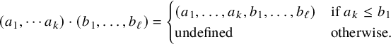 $$ \begin{align*}(a_1,\cdots a_k)\cdot (b_1,\ldots,b_\ell)=\begin{cases}(a_1,\ldots,a_k,b_1,\ldots,b_\ell)& \text{if }a_k\le b_1\\\text{undefined}&\text{otherwise.}\end{cases}\end{align*} $$
This makes $\mathsf {WInc}$
into a graded right-cancellative monoid with
$\mathsf {WInc}$
into a graded right-cancellative monoid with $\operatorname {Last}((b_1,\ldots ,b_k))=\{b_k\}$
and
$\operatorname {Last}((b_1,\ldots ,b_k))=\{b_k\}$
and $\operatorname {Fac}((b_1,\ldots ,b_k))=\{(b_1,\ldots ,b_k)\}$
.
$\operatorname {Fac}((b_1,\ldots ,b_k))=\{(b_1,\ldots ,b_k)\}$
.
Let $\mathsf {R}_{i}^{\infty }$
be the truncation operator defined by
$\mathsf {R}_{i}^{\infty }$
be the truncation operator defined by $\mathsf {R}_{i}^{\infty }(f)=f(x_1,\ldots ,x_{i-1},x_i,0,0,\ldots )$
. It is the limit of
$\mathsf {R}_{i}^{\infty }(f)=f(x_1,\ldots ,x_{i-1},x_i,0,0,\ldots )$
. It is the limit of $\mathsf {R}_{i}^{m}(f)$
when m tends to infinity, as these polynomials clearly become stable equal to
$\mathsf {R}_{i}^{m}(f)$
when m tends to infinity, as these polynomials clearly become stable equal to $\mathsf {R}_{i}^{\infty }(f)$
.
$\mathsf {R}_{i}^{\infty }(f)$
.
Definition 5.2 (Slide extractor).
Define the slide extractor to be
which for $f\in \operatorname {Pol}$
is given concretely by
$f\in \operatorname {Pol}$
is given concretely by
We have ![]() , thus
, thus ![]() if
if $i>j$
, and so
$i>j$
, and so ![]() . Thus, the operators
. Thus, the operators ![]() give a representation of
give a representation of $\mathsf {WInc}$
, and with
$\mathsf {WInc}$
, and with ![]() , we have a dd-pair
, we have a dd-pair ![]() .
.
Theorem 5.3. Slide polynomials ![]() form the unique dual family of polynomials to the dd-pair
form the unique dual family of polynomials to the dd-pair ![]() . Thus, for
. Thus, for $(b_1\le \cdots \le b_k)\in \mathsf {WInc}$
, we have
$(b_1\le \cdots \le b_k)\in \mathsf {WInc}$
, we have
Note that the formula above can be checked directly by a simple computation, as we have an explicit expansion for slide polynomials. We will instead use Theorem 2.20, and this will come as a consequence.
Definition 5.4. Define a linear map ![]() as
as
Explicitly, ![]() vanishes outside of
vanishes outside of $\operatorname {Pol}_i$
and is defined on monomials of
$\operatorname {Pol}_i$
and is defined on monomials of $\operatorname {Pol}_i$
by
$\operatorname {Pol}_i$
by
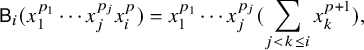
where $p_j>0$
or
$p_j>0$
or $j=0$
.
$j=0$
.
Proposition 5.5. The ![]() are creation operators for
are creation operators for ![]() : on
: on $\operatorname {Pol}^+$
, we have
$\operatorname {Pol}^+$
, we have
Proof. On the one hand, since $\mathsf {R}_{1}^{\infty }=\operatorname {ev}_{0}$
vanishes on
$\mathsf {R}_{1}^{\infty }=\operatorname {ev}_{0}$
vanishes on $\operatorname {Pol}^+$
, we obtain by telescoping
$\operatorname {Pol}^+$
, we obtain by telescoping
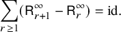 $$ \begin{align} \sum_{r\geq 1} (\mathsf{R}_{r+1}^{\infty}-\mathsf{R}_{r}^{\infty})=\mathrm{id}. \end{align} $$
Now, we compute that
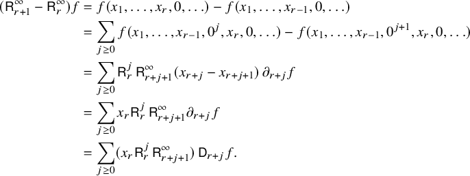
Summing this over all r, the coefficient of ![]() is then
is then ![]() .
.
Our next result, Proposition 5.6, applied to increasing sequences $1\le a_1\le \cdots \le a_k$
implies that the slide polynomials are the dual family of polynomials to
$1\le a_1\le \cdots \le a_k$
implies that the slide polynomials are the dual family of polynomials to ![]() . We note that although we could have taken an alternate choice of creation operators such as
. We note that although we could have taken an alternate choice of creation operators such as ![]() (because
(because ![]() ), Proposition 5.6 shows surprisingly that composites of the
), Proposition 5.6 shows surprisingly that composites of the ![]() operators construct slide polynomials even for non-decreasing sequences – a property not formally guaranteed by the slide polynomials being the dual family to
operators construct slide polynomials even for non-decreasing sequences – a property not formally guaranteed by the slide polynomials being the dual family to ![]() . This additional property of
. This additional property of ![]() will be needed later in Proposition 5.7 to recover the slide expansions of Schubert and forest polynomials.
will be needed later in Proposition 5.7 to recover the slide expansions of Schubert and forest polynomials.
Proposition 5.6. For any sequence $(a_1,\ldots ,a_k)$
with
$(a_1,\ldots ,a_k)$
with $a_i\ge 1$
, we have
$a_i\ge 1$
, we have
Proof. By induction, it is enough to show that if $a=(a_1,\dots ,a_k)$
, then
$a=(a_1,\dots ,a_k)$
, then ![]() for any
for any $p\geq 1$
. In what follows, we write
$p\geq 1$
. In what follows, we write $\lambda ^\ell $
for the length
$\lambda ^\ell $
for the length $\ell $
sequence
$\ell $
sequence $\lambda ,\ldots ,\lambda $
. For
$\lambda ,\ldots ,\lambda $
. For ![]() , we define a set
, we define a set
 $$ \begin{align*}A_{(i_1,\ldots,i_k)}=\begin{cases}\varnothing & \text{if }i_k>p\\\{(i_1,\ldots,i_\ell,i^{k-\ell+1})\;|\; i_\ell<i\le p\}&\text{if }(i_1,\ldots,i_k)=(i_1,\ldots,i_\ell,p^{k-\ell})\text{ with }i_\ell<p.\end{cases}\end{align*} $$
Then by definition of ![]() and the slide polynomials as generating functions, it suffices to show that
and the slide polynomials as generating functions, it suffices to show that
First, the $A_{(i_1,\ldots ,i_k)}$
are obviously disjoint sets, the elements being uniquely determined by the longest initial subsequence of
$A_{(i_1,\ldots ,i_k)}$
are obviously disjoint sets, the elements being uniquely determined by the longest initial subsequence of $(i_1,\ldots ,i_k)$
strictly less than p, so the union is disjoint as claimed. Next, we show
$(i_1,\ldots ,i_k)$
strictly less than p, so the union is disjoint as claimed. Next, we show ![]() . Indeed, since
. Indeed, since ![]() ,
,
-
• if
$\ell <k$
, we must have
$a_k\ge p$
, and so , and -
• if
$\ell =k$
, then because
$p>i_\ell $
, we also have .


The other sequences $(i_1,\ldots ,i_\ell ,i^{k-\ell +1})\in A_{(i_1,\ldots ,i_k)}$
must lie in
$(i_1,\ldots ,i_\ell ,i^{k-\ell +1})\in A_{(i_1,\ldots ,i_k)}$
must lie in ![]() as well since it is a smaller sequence with the same indices at which strict ascents occur.
as well since it is a smaller sequence with the same indices at which strict ascents occur.
Finally, every sequence in ![]() can be written as
can be written as $(i_1,\ldots ,i_\ell ,i^{k-\ell +1})$
for some
$(i_1,\ldots ,i_\ell ,i^{k-\ell +1})$
for some $0\le \ell \le k$
and
$0\le \ell \le k$
and $i_\ell <i\le p$
, and we claim that
$i_\ell <i\le p$
, and we claim that ![]() . Note that because the last
. Note that because the last $k-\ell +1$
elements of
$k-\ell +1$
elements of $(i_1,\ldots ,i_\ell ,i^{k-\ell +1})$
are equal, we have
$(i_1,\ldots ,i_\ell ,i^{k-\ell +1})$
are equal, we have $a_{k-\ell }\ge a_{k-\ell +1}\ge \cdots \ge a_k\ge p$
. Therefore, as
$a_{k-\ell }\ge a_{k-\ell +1}\ge \cdots \ge a_k\ge p$
. Therefore, as $(i_1,\ldots ,i_\ell ,p^{k-\ell +1})$
has the same indices of strict ascents as
$(i_1,\ldots ,i_\ell ,p^{k-\ell +1})$
has the same indices of strict ascents as $(i_1,\ldots ,i_\ell ,i^{k-\ell +1})$
, we have the sequence
$(i_1,\ldots ,i_\ell ,i^{k-\ell +1})$
, we have the sequence ![]() , which in particular implies that
, which in particular implies that ![]() .
.
We can now prove Theorem 5.3.
Proof of Theorem 5.3.
We have the code map $c:\mathsf {WInc}\to \mathsf {Codes}$
given by
$c:\mathsf {WInc}\to \mathsf {Codes}$
given by $c(a_1\le \cdots \le a_k)=(c_1,c_2,\ldots )$
, where
$c(a_1\le \cdots \le a_k)=(c_1,c_2,\ldots )$
, where $c_i=\#\{j\;|\; a_j=i\}$
. It satisfies the conditions of Definition 2.19. The
$c_i=\#\{j\;|\; a_j=i\}$
. It satisfies the conditions of Definition 2.19. The ![]() are shown to be creation operators for
are shown to be creation operators for ![]() in Proposition 5.5. We can thus apply Theorem 2.20, which gives us that the dual family to
in Proposition 5.5. We can thus apply Theorem 2.20, which gives us that the dual family to ![]() is unique, forms a basis of
is unique, forms a basis of $\operatorname {Pol}$
, and is given explicitly by
$\operatorname {Pol}$
, and is given explicitly by ![]() for
for $(a_1,\ldots ,a_k)\in \mathsf {WInc}$
. These are precisely the slide polynomials by Proposition 5.6, which concludes the proof.
$(a_1,\ldots ,a_k)\in \mathsf {WInc}$
. These are precisely the slide polynomials by Proposition 5.6, which concludes the proof.
5.3 Applications
We first show how to recover the slide expansions of Schubert polynomials and forest polynomials, the first one being the celebrated BJS formula [Reference Billey, Jockusch and Stanley6].
Proposition 5.7. We have the following expansions for any $w\in S_\infty $
and any
$w\in S_\infty $
and any ![]() :
:
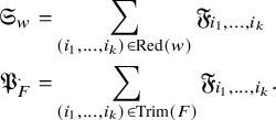
Proof. Note that ![]() . Because
. Because ![]() , we can either absorb all or all but one
, we can either absorb all or all but one $\mathsf {R}_{i+1}$
into
$\mathsf {R}_{i+1}$
into ![]() to obtain
to obtain
Then Proposition 5.5 shows that ![]() are creation operators for
are creation operators for $\partial _i$
and for
$\partial _i$
and for ![]() . We can then use Theorem 2.20 for the corresponding dd-pairs:
. We can then use Theorem 2.20 for the corresponding dd-pairs:
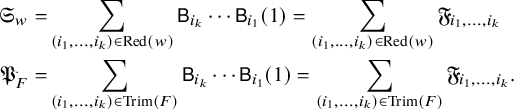
Because slide polynomials are a basis of $\operatorname {Pol}$
, Proposition 2.11 implies the following.
$\operatorname {Pol}$
, Proposition 2.11 implies the following.
Corollary 5.8. The slide expansion of a degree k homogeneous polynomial $f\in \operatorname {Pol}$
is given by
$f\in \operatorname {Pol}$
is given by
Example 5.9. Consider $f=\mathfrak {S}_{21534}=x_1x_3^2 + x_1x_2x_3 + x_1^2x_3 + x_1x_2^2 + x_1^2x_2 + x_1^3$
. Figure 7 shows applications of slide extractors in weakly decreasing order of the indices. Corollary 5.8 says
$f=\mathfrak {S}_{21534}=x_1x_3^2 + x_1x_2x_3 + x_1^2x_3 + x_1x_2^2 + x_1^2x_2 + x_1^3$
. Figure 7 shows applications of slide extractors in weakly decreasing order of the indices. Corollary 5.8 says
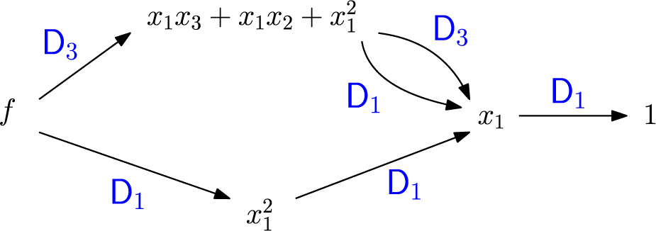
Figure 7 Repeatedly applying ![]() s to extract slide coefficients for
s to extract slide coefficients for $f=\mathfrak {S}_{21534}$
.
$f=\mathfrak {S}_{21534}$
.
As an application, let us reprove the positivity of slide multiplication established combinatorially by Assaf–Searles [Reference Assaf and Searles3, Theorem 5.1] using the ‘quasi-shuffle product’. In contrast, we use a Leibniz rule for the ![]() that makes the positivity manifest. We shall not pursue unwinding our approach to make the combinatorics explicit.
that makes the positivity manifest. We shall not pursue unwinding our approach to make the combinatorics explicit.
Lemma 5.10.
![]() is a slide polynomial or
is a slide polynomial or $0$
.
$0$
.
Proof. Assume the result is true for all lower degree slide polynomials. By Theorem 5.3, it suffices to show that ![]() for all i, except at most one for which
for all i, except at most one for which ![]() for some
for some $b\in \mathsf {Winc}$
.
$b\in \mathsf {Winc}$
.
Let $a=(a_1,\ldots ,a_k)\in \mathsf {WInc}$
, and let
$a=(a_1,\ldots ,a_k)\in \mathsf {WInc}$
, and let $a'=(a_1,\ldots ,a_{k-1})\in \mathsf {WInc}$
. The identity
$a'=(a_1,\ldots ,a_{k-1})\in \mathsf {WInc}$
. The identity
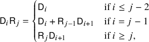
together with Theorem 5.3 implies that
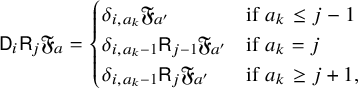
and we conclude by the inductive hypothesis.
Corollary 5.11. The product of slide polynomials is slide-positive.
Proof. By Corollary 5.8, it suffices to show that ![]() is slide positive if each of
is slide positive if each of $f,g$
are slide positive. For
$f,g$
are slide positive. For $f,g\in \operatorname {Pol}$
we have a ‘Leibniz rule’ that says,
$f,g\in \operatorname {Pol}$
we have a ‘Leibniz rule’ that says,
If $f,g$
are slide polynomials, then by Theorem 5.3, we know that
$f,g$
are slide polynomials, then by Theorem 5.3, we know that ![]() are either slide polynomials or
are either slide polynomials or $0$
, so from Lemma 5.10, the slide positivity follows by induction.
$0$
, so from Lemma 5.10, the slide positivity follows by induction.
Our second application is to determine the inverse of the ‘Slide Kostka’ matrix (i.e., express monomials in terms of slide polynomials). This was obtained by the first and third author via involved combinatorial means in [Reference Nadeau and Tewari24, Theorem 5.2].
To state the result, fix a sequence $a=(a_1,\dots ,a_k)\in \mathsf {WInc}$
. Group equal terms and write
$a=(a_1,\dots ,a_k)\in \mathsf {WInc}$
. Group equal terms and write $a=(M_1^{m_1},M_2^{m_2},\ldots ,M_p^{m_p})$
, with
$a=(M_1^{m_1},M_2^{m_2},\ldots ,M_p^{m_p})$
, with $M_1<\cdots <M_p$
. Set
$M_1<\cdots <M_p$
. Set ![]() . For a fixed
. For a fixed $i\in \{1,\ldots ,p\}$
, define
$i\in \{1,\ldots ,p\}$
, define $E_i(a)\subset \mathsf {WInc}$
by
$E_i(a)\subset \mathsf {WInc}$
by
 $$\begin{align*}E_i(a)=\{(b_1,\dots,b_{m_i})\;|\; b_{j+1}-b_j\in\{0,1\}=0 \text{ and } b_1>M_{i-1}\}, \end{align*}$$
where ![]() . Let
. Let $n(b)=M_i-b_1$
for
$n(b)=M_i-b_1$
for $b\in E_i(a)$
, which counts the number of j such that
$b\in E_i(a)$
, which counts the number of j such that $b_{j+1}-b_j=1$
for
$b_{j+1}-b_j=1$
for $1\leq j\leq m_i$
. Finally, let
$1\leq j\leq m_i$
. Finally, let
 $$\begin{align*}E(a)=\{b\in \mathsf{WInc}\;|\; b=e^1\cdots e^{p} \text{ where each } e^i\in E_i(a)\}, \end{align*}$$
To $b=e^1\cdots e^{p}\in E(a)$
, assign the sign
$b=e^1\cdots e^{p}\in E(a)$
, assign the sign $\epsilon (b)=(-1)^{\sum _i n(e^i)}$
. For instance, if
$\epsilon (b)=(-1)^{\sum _i n(e^i)}$
. For instance, if $a=(2,4,4)$
, then
$a=(2,4,4)$
, then $E(a)=\{(2,4,4),(1,4,4),(2,3,4),(1,3,4),(2,3,3),(1,3,3)\}$
with respective signs
$E(a)=\{(2,4,4),(1,4,4),(2,3,4),(1,3,4),(2,3,3),(1,3,3)\}$
with respective signs $1,-1,-1,1,-1,1$
.
$1,-1,-1,1,-1,1$
.
Corollary 5.12 [Reference Nadeau and Tewari24, Theorem 5.2].
The slide expansion of any monomial is signed multiplicity-free. Explicitly, for any $a=(a_1,\dots ,a_k)\in \mathsf {WInc}$
, we have
$a=(a_1,\dots ,a_k)\in \mathsf {WInc}$
, we have
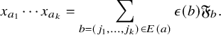
Sketch of the proof.
By Corollary 5.8, the coefficient of ![]() for
for $(j_1,\dots ,j_k)\in \mathsf {WInc}$
in (5.4) is given by
$(j_1,\dots ,j_k)\in \mathsf {WInc}$
in (5.4) is given by ![]() . By Definition 5.2, we can compute
. By Definition 5.2, we can compute
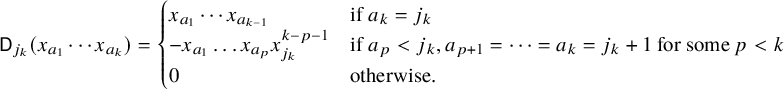
Thus, ![]() is either
is either $0$
or another monomial up to sign, which shows that the expansion is signed multiplicity-free. More precisely, let
$0$
or another monomial up to sign, which shows that the expansion is signed multiplicity-free. More precisely, let $E'(a)$
be the set of
$E'(a)$
be the set of $b=(j_1,\dots ,j_k)$
such that
$b=(j_1,\dots ,j_k)$
such that ![]() has nonzero coefficient in (5.4). Then it follows that
has nonzero coefficient in (5.4). Then it follows that $b\in E'(a)$
either if
$b\in E'(a)$
either if $j_k=a_k$
and
$j_k=a_k$
and $(j_1,\dots ,j_{k-1})\in E'(a_1,\dots ,a_{k-1})$
, or if
$(j_1,\dots ,j_{k-1})\in E'(a_1,\dots ,a_{k-1})$
, or if $j_k+1=a_k$
, there exists
$j_k+1=a_k$
, there exists $p<k$
such that
$p<k$
such that $a_p<j_k$
,
$a_p<j_k$
, $a_{p+1}=\dots =a_{k}=j_k+1$
, and
$a_{p+1}=\dots =a_{k}=j_k+1$
, and $(j_1,\dots ,j_{k-1})\in E'(a_1,\dots ,a_{p},j_k^{k-p-1})$
. We let the interested reader show that
$(j_1,\dots ,j_{k-1})\in E'(a_1,\dots ,a_{p},j_k^{k-p-1})$
. We let the interested reader show that $E(a)$
satisfies the same recursion, so that
$E(a)$
satisfies the same recursion, so that $E(a)=E'(a)$
by induction. The sign is then readily checked.
$E(a)=E'(a)$
by induction. The sign is then readily checked.
5.4 m-slides interpolating between monomials and slides
To conclude this article, we briefly describe how the results generalize to monomials, m-slide polynomials and m-forest polynomials. The proofs are nearly identical to the case $m=1$
, so we omit them.
$m=1$
, so we omit them.
For a sequence $a=(a_1,\ldots ,a_k)$
with
$a=(a_1,\ldots ,a_k)$
with $a_i\ge 1$
, we define the set of m-compatible sequences
$a_i\ge 1$
, we define the set of m-compatible sequences
The m-slide polynomial [Reference Nadeau, Spink and Tewari22, Section 8] is the generating function
For fixed $a=(a_1,\dots ,a_k)$
and m sufficiently large, we have
$a=(a_1,\dots ,a_k)$
and m sufficiently large, we have ![]() if
if $(a_1,\ldots ,a_k)\in \mathsf {WInc}$
and
$(a_1,\ldots ,a_k)\in \mathsf {WInc}$
and $0$
otherwise. So we may consider monomials as
$0$
otherwise. So we may consider monomials as $\infty $
-slide polynomials, and the m-slide polynomials as interpolating between slide polynomials and monomials.
$\infty $
-slide polynomials, and the m-slide polynomials as interpolating between slide polynomials and monomials.
Proposition 5.13. For $i\geq 1$
, consider the m-slide extractors
$i\geq 1$
, consider the m-slide extractors ![]() defined as
defined as ![]() For
For $(b_1\le \cdots \le b_k)\in \mathsf {WInc}$
, we have
$(b_1\le \cdots \le b_k)\in \mathsf {WInc}$
, we have
Consequently, the m-slide expansion of a degree k homogeneous polynomial $f\in \operatorname {Pol}$
is given by
$f\in \operatorname {Pol}$
is given by
Example 5.14. Taking $f=\mathfrak {S}_{21534}=x_1x_3^2 + x_1x_2x_3 + x_1^2x_3 + x_1x_2^2 + x_1^2x_2 + x_1^3$
as in Example 5.9, we see, for instance, that
$f=\mathfrak {S}_{21534}=x_1x_3^2 + x_1x_2x_3 + x_1^2x_3 + x_1x_2^2 + x_1^2x_2 + x_1^3$
as in Example 5.9, we see, for instance, that
which in turn means the coefficient of $x_1x_2^2$
in
$x_1x_2^2$
in $\mathfrak {S}_{21534}$
is
$\mathfrak {S}_{21534}$
is $1$
.
$1$
.
Theorem 5.15. Consider m-slide creation operators ![]() that vanish outside of
that vanish outside of $\operatorname {Pol}_a$
, and are defined on monomials of
$\operatorname {Pol}_a$
, and are defined on monomials of $\operatorname {Pol}_a$
by
$\operatorname {Pol}_a$
by
where $j<a$
and
$j<a$
and $p_j>0$
(or
$p_j>0$
(or $j=0$
) and
$j=0$
) and $p\geq 0$
. The following hold.
$p\geq 0$
. The following hold.
-
(1) For
$a=(a_1,\dots ,a_k)$
any sequence with
$a_i\ge 1$
, we have In particular, for any sequence
$(b_1,\ldots ,b_k)$
with
$b_i\ge 1$
, we have -
(2) We have
on
$\operatorname {Pol}^+$
(i.e., are creation operators for both m-slides and m-forest polynomials). In particular,


Remark 5.16. For $m=\infty $
, we recover the rather straightforward dd-pair
$m=\infty $
, we recover the rather straightforward dd-pair ![]() for monomials, where for
for monomials, where for $a_k>1$
, we have
$a_k>1$
, we have ![]() , and the creation operators
, and the creation operators ![]() .
.
Acknowledgements
We are very grateful to Dave Anderson, Sara Billey, Igor Pak, Greta Panova, Brendan Pawlowski, Richard Stanley and Josh Swanson for enlightening discussions. We would also like to thank the anonymous referees for helpful suggestions to improve exposition.
Competing interest
The authors have no competing interests to declare.
Financial Support
Philippe Nadeau was partially supported by French ANR grant ANR-19-CE48-0011 (COMBINÉ). Hunter Spink and Vasu Tewari acknowledge the support of the Natural Sciences and Engineering Research Council of Canada (NSERC), respectively [RGPIN-2024-04181] and [RGPIN-2024-05433].


 Open access