


1 Introduction
In [Reference Bousseau, Brini and van Garrel11] Bousseau, Brini and van Garrel discovered a surprising relationship between two at first sight quite different curve counting theories:
-
• Logarithmic Gromov–Witten theory of a Looijenga pair
which is a rational smooth projective surfaces S together with an anticanonical singular nodal curve $$ \begin{align*} (S \hspace{0.2ex}|\hspace{0.2ex} D_1+\ldots +D_l) \end{align*} $$
$D_1+\ldots + D_l$
. To this datum one can associate a Gromov–Witten invariant enumerating genus g, class
$$ \begin{align*} \mathsf{LGW}_{g,\mathbf{\hat{c}},\unicode{x3b2}}(S \hspace{0.2ex}|\hspace{0.2ex} D_1+\ldots +D_l) \in \mathbb{Q} \end{align*} $$
$\unicode{x3b2} $
stable logarithmic maps to
$(S \hspace {0.2ex}|\hspace {0.2ex} D_1+\ldots +D_l)$
with maximum tangency along each irreducible component
$D_i$
. Additionally, there are
$l-1$
interior markings with a point condition and an insertion of the top Chern class of the Hodge bundle. The tangency order of the markings along
$D_1,\ldots ,D_l$
is recorded in a matrix
$\mathbf {\hat {c}}$
.
$$ \begin{align*} (S \hspace{0.2ex}|\hspace{0.2ex} D_1+\ldots +D_l) \end{align*} $$
$D_1+\ldots + D_l$
. To this datum one can associate a Gromov–Witten invariant enumerating genus g, class
$$ \begin{align*} \mathsf{LGW}_{g,\mathbf{\hat{c}},\unicode{x3b2}}(S \hspace{0.2ex}|\hspace{0.2ex} D_1+\ldots +D_l) \in \mathbb{Q} \end{align*} $$
$\unicode{x3b2} $
stable logarithmic maps to
$(S \hspace {0.2ex}|\hspace {0.2ex} D_1+\ldots +D_l)$
with maximum tangency along each irreducible component
$D_i$
. Additionally, there are
$l-1$
interior markings with a point condition and an insertion of the top Chern class of the Hodge bundle. The tangency order of the markings along
$D_1,\ldots ,D_l$
is recorded in a matrix
$\mathbf {\hat {c}}$
.
-
• Open Gromov–Witten theory of a toric triple
consisting of the toric Calabi–Yau threefold X and a collection of framed Aganagic–Vafa Lagrangian submanifolds
$$ \begin{align*} \big(X,(L_i,\mathsf{f}_i)_{i=1}^k\big) \end{align*} $$
$(L_i,\mathsf {f}_i)$
. To this data one can associate open Gromov–Witten invariants enumerating genus g, class
$$ \begin{align*} \mathsf{OGW}_{g,((w_1), \ldots, (w_k)),\unicode{x3b2}'}(X,(L_i,\mathsf{f}_i)_{i=1}^k) \in \mathbb{Q} \end{align*} $$
$\unicode{x3b2} '$
stable maps to X from Riemann surfaces with k boundaries, each wrapping one of the Lagrangian submanifolds
$L_i$
exactly
$w_i$
times.


It was conjectured in [Reference Bousseau, Brini and van Garrel11] that starting from a Looijenga pair, one can geometrically engineer a toric triple so that the above two curve counts turn out to be essentially equal.
Conjecture 1.1 [Reference Bousseau, Brini and van Garrel11, Conjecture 1.3].
Let $(S \hspace {0.2ex}|\hspace {0.2ex} D_1+\ldots +D_l)$
be a Looijenga pair and
$(S \hspace {0.2ex}|\hspace {0.2ex} D_1+\ldots +D_l)$
be a Looijenga pair and $\unicode{x3b2} $
an effective curve class in S satisfying some technical conditions. Then there exists a toric triple
$\unicode{x3b2} $
an effective curve class in S satisfying some technical conditions. Then there exists a toric triple $(X,(L_i,\mathsf {f}_i)_{i=1}^{l-1})$
and an effective curve class
$(X,(L_i,\mathsf {f}_i)_{i=1}^{l-1})$
and an effective curve class $\beta '$
in X such that
$\beta '$
in X such that
 $$ \begin{align} \sum_{g\geq 0} \hbar^{2g-2} ~ \mathsf{OGW}_{g,\mathbf{c},\unicode{x3b2}'}(X, (L_i,\mathsf{f}_{i})_{i=1}^{l-1}) = \bigg(\prod_{i=1}^{l-1} \frac{(-1)^{D_i \cdot \unicode{x3b2}}}{D_i \cdot \unicode{x3b2}} \bigg) \frac{(-1)^{D_l \cdot \unicode{x3b2} +1}}{2 \sin \tfrac{(D_l \cdot \unicode{x3b2})\hbar}{2}} \,\sum_{g\geq 0} \hbar^{2g-1} \mathsf{LGW}_{g,\mathbf{\hat{c}},\unicode{x3b2}}(S \hspace{0.2ex}|\hspace{0.2ex} D_1+\ldots+D_l), \end{align} $$
where $\mathbf {c}$
is obtained from the contact datum
$\mathbf {c}$
is obtained from the contact datum $\mathbf {\hat {c}}$
by deleting the
$\mathbf {\hat {c}}$
by deleting the $l-1$
interior markings and the marking with tangency along
$l-1$
interior markings and the marking with tangency along $D_l$
.
$D_l$
.
For $l=1$
, the right-hand side of (1.1) reduces to the generating series of ordinary Gromov–Witten invariants of X in which case the conjecture has already been proven in [Reference van Garrel, Nabijou and Schuler45, Theorem D]. In this paper, we investigate the case of two-component Looijenga pairs
$l=1$
, the right-hand side of (1.1) reduces to the generating series of ordinary Gromov–Witten invariants of X in which case the conjecture has already been proven in [Reference van Garrel, Nabijou and Schuler45, Theorem D]. In this paper, we investigate the case of two-component Looijenga pairs $(S \hspace {0.2ex}|\hspace {0.2ex} D_1+D_2)$
, and as another application of the main result in [Reference van Garrel, Nabijou and Schuler45], we will establish Conjecture 1.1 for these geometries.
$(S \hspace {0.2ex}|\hspace {0.2ex} D_1+D_2)$
, and as another application of the main result in [Reference van Garrel, Nabijou and Schuler45], we will establish Conjecture 1.1 for these geometries.
1.1 Logarithmic-open correspondence
Consider a two-component Looijenga pair $(S \hspace {0.2ex}|\hspace {0.2ex} D_1+D_2)$
together with an effective curve class
$(S \hspace {0.2ex}|\hspace {0.2ex} D_1+D_2)$
together with an effective curve class $\unicode{x3b2} $
in S. We will impose
$\unicode{x3b2} $
in S. We will impose
Assumption ★. $(S \hspace {0.2ex}|\hspace {0.2ex} D_1+D_2)$
and
$(S \hspace {0.2ex}|\hspace {0.2ex} D_1+D_2)$
and $\unicode{x3b2} $
satisfy
$\unicode{x3b2} $
satisfy
-
•
$D_i \cdot \unicode{x3b2}>0$
,
$i\in \{1,2\}$
, -
•
$D_2 \cdot D_2\geq 0$
, -
•
$(S\hspace {0.2ex}|\hspace {0.2ex} D_1)$
deforms into a pair
$(S^{\prime } \hspace {0.2ex}|\hspace {0.2ex} D_1^{\prime })$
with
$S^{\prime }$
a smooth projective toric surface and
$D_1^{\prime }$
a toric hypersurface.Footnote
1


Moreover, we denote by $\mathbf {\hat {c}}$
the following contact datum along
$\mathbf {\hat {c}}$
the following contact datum along $D_1+D_2$
where we assume $n\geq m$
and
$n\geq m$
and $c_i>0$
for all
$c_i>0$
for all $i\in \{1,\ldots ,n\}$
. This means there are m interior markings, n markings tangent to
$i\in \{1,\ldots ,n\}$
. This means there are m interior markings, n markings tangent to $D_1$
and an additional marking with maximum tangency along
$D_1$
and an additional marking with maximum tangency along $D_2$
. We set
$D_2$
. We set

Especially, note that we impose a point condition at all m interior markings. Our main result is the following logarithmic to open correspondence.
Theorem 1.2 (Theorem 2.9).
Assuming ★ there is a toric triple $(X,L,\mathsf {f})$
(see Construction 2.8) and a curve class
$(X,L,\mathsf {f})$
(see Construction 2.8) and a curve class $\unicode{x3b2} ^{\prime }$
in X satisfying
$\unicode{x3b2} ^{\prime }$
in X satisfying
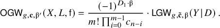
 $$ \begin{align} \sum_{g\geq 0} \hbar^{2g-2} ~ \mathsf{OGW}_{g,\mathbf{c},\unicode{x3b2}^{\prime}}(X,L,\mathsf{f}) = \frac{(-1)^{D_1 \cdot \unicode{x3b2}}}{m! \, \textstyle{\prod_{i=0}^{m-1}} c_{n-i}} \, \frac{(-1)^{D_2 \cdot \unicode{x3b2} +1}}{2 \sin \tfrac{(D_2 \cdot \unicode{x3b2})\hbar}{2}} ~ \sum_{g\geq 0} \hbar^{2g-1} ~ \mathsf{LGW}_{g,\mathbf{\hat{c}},\unicode{x3b2}}(S \hspace{0.2ex}|\hspace{0.2ex} D_1+D_2) \,. \end{align} $$
The specialisation of the above correspondence to the case $m=n=1$
immediately gives
$m=n=1$
immediately gives

1.2 Topological vertex
Computing Gromov–Witten invariants of logarithmic Calabi–Yau surfaces is usually a rather tedious endeavour. In higher genus with the presence of a $\unicode{x3bb} _g$
insertion, the only general tools available are scattering diagrams and tropical correspondence theorems [Reference Bousseau9, Reference Bousseau7, Reference Bousseau10, Reference Kennedy-Hunt, Shafi and Kumaran23].
$\unicode{x3bb} _g$
insertion, the only general tools available are scattering diagrams and tropical correspondence theorems [Reference Bousseau9, Reference Bousseau7, Reference Bousseau10, Reference Kennedy-Hunt, Shafi and Kumaran23].
As an application of Theorem 1.2 we obtain a new – and highly efficient – means for computing logarithmic Gromov Witten invariants of Looijenga pairs. Since open Gromov–Witten invariants can be computed using the topological vertex [Reference Aganagic, Klemm, Mariño and Vafa4, Reference Li, Liu, Liu and Zhou30], the same method can be applied to determine the opposite side of our correspondence theorem.
1.3 BPS integrality
In general, Gromov–Witten invariants are rational numbers. However, in many cases, they are expected to exhibit underlying integral BPS type invariants. For open Gromov–Witten invariants, this behaviour was first observed by Labastida–Mariño–Ooguri–Vafa [Reference Ooguri and Vafa41, Reference Labastida and Mariño26, Reference Labastida, Mariño and Vafa27, Reference Mariño and Vafa39], was studied extensively in explicit examples by Luo–Zhu [Reference Luo and Zhu35, Reference Zhu47, Reference Zhu48] and got recently proven by Yu [Reference Yu46] for general toric targets. Hence, as a corollary of our main result Theorem 1.2, we find that logarithmic invariants feature the same property.
Theorem 1.5 (Theorem 5.5).
The logarithmic Gromov–Witten invariants (1.2) of a two-component Looijenga pair satisfying Assumption ★ exhibit BPS integrality.
In Section 5.2, we spell this statement out in more detail. We conjecture that the above observation holds without imposing Assumption ★ as well (Conjecture 5.4).
1.4 Strategy
The proof of Theorem 1.2 splits into several steps which partly have already been carried out elsewhere:
In [Reference van Garrel, Nabijou and Schuler45], van Garrel, Nabijou and the author prove a comparison statement between the Gromov–Witten theory of $(S \hspace {0.2ex}|\hspace {0.2ex} D_1+D_2)$
and
$(S \hspace {0.2ex}|\hspace {0.2ex} D_1+D_2)$
and $(\mathcal {O}_S(-D_2) \hspace {0.2ex}|\hspace {0.2ex} D_1)$
. Together with a result of Fang and Liu [Reference Fang and Liu14] expressing the open Gromov–Witten invariants of a toric triple
$(\mathcal {O}_S(-D_2) \hspace {0.2ex}|\hspace {0.2ex} D_1)$
. Together with a result of Fang and Liu [Reference Fang and Liu14] expressing the open Gromov–Witten invariants of a toric triple $(X,L,\mathsf {f})$
as descendant invariants of X, it is therefore sufficient to prove a formula for relative Gromov–Witten invariants of
$(X,L,\mathsf {f})$
as descendant invariants of X, it is therefore sufficient to prove a formula for relative Gromov–Witten invariants of $(\mathcal {O}_S(-D_2) \hspace {0.2ex}|\hspace {0.2ex} D_1)$
in terms of descendant invariants of
$(\mathcal {O}_S(-D_2) \hspace {0.2ex}|\hspace {0.2ex} D_1)$
in terms of descendant invariants of $X=\operatorname *{\mathrm {Tot}}\mathcal {O}_S(-D_2)|_{S \setminus D_1}$
in order to establish Theorem 1.2. We will prove such a relation in Section 3 in case there are no interior markings (
$X=\operatorname *{\mathrm {Tot}}\mathcal {O}_S(-D_2)|_{S \setminus D_1}$
in order to establish Theorem 1.2. We will prove such a relation in Section 3 in case there are no interior markings ( $m=0$
). Later in Section 4, we will reduce the general case (
$m=0$
). Later in Section 4, we will reduce the general case ( $m\geq 0$
) to the one proven earlier.
$m\geq 0$
) to the one proven earlier.
1.5 Context & Prospects
1.5.1 Stable maps to Looijenga pairs
Conjecture 1.1 was formulated by Bousseau, Brini and van Garrel in [Reference Bousseau, Brini and van Garrel11], motivated by a direct calculation and comparison of both sides of the correspondence. More precisely, in loc. cit. Conjecture 1.1 was established for all so-called tame Looijenga pairs (up to a possible relabelling of boundary components), and later in [Reference Krattenthaler25, Reference Brini and Schuler12], the list of examples was extended to encompass all quasi-tame pairs as well. When $l=2$
, a Looijenga pair
$l=2$
, a Looijenga pair $(S\hspace {0.2ex}|\hspace {0.2ex} D_1 + D_2)$
is called tame if
$(S\hspace {0.2ex}|\hspace {0.2ex} D_1 + D_2)$
is called tame if $D_i\cdot D_i>0$
,
$D_i\cdot D_i>0$
, $i\in \{1,2\}$
, and quasi-tame if
$i\in \{1,2\}$
, and quasi-tame if $\operatorname *{\mathrm {Tot}} \mathcal {O}_{S}(-D_1) \oplus \mathcal {O}_{S}(-D_2)$
deforms to the total space of line bundles associated to a tame pair. It turns out there is only a finite number of such quasi-tame Looijenga pairs [Reference Bousseau, Brini and van Garrel11, Section 2.4], and for
$\operatorname *{\mathrm {Tot}} \mathcal {O}_{S}(-D_1) \oplus \mathcal {O}_{S}(-D_2)$
deforms to the total space of line bundles associated to a tame pair. It turns out there is only a finite number of such quasi-tame Looijenga pairs [Reference Bousseau, Brini and van Garrel11, Section 2.4], and for $l=2$
, one can check that apart from
$l=2$
, one can check that apart from $\mathbb {F}_0(2,2)$
, all of them satisfy Assumption ★.Footnote
2
Thus, regarding two-component Looijenga pairs, Corollary 1.3 covers all cases previously known in the literature with the exception of
$\mathbb {F}_0(2,2)$
, all of them satisfy Assumption ★.Footnote
2
Thus, regarding two-component Looijenga pairs, Corollary 1.3 covers all cases previously known in the literature with the exception of $\mathbb {F}_0(2,2)$
. Among these is the quasi-tame pair
$\mathbb {F}_0(2,2)$
. Among these is the quasi-tame pair $\mathrm {dP}_3(0,2)$
. For this geometry, an explicit formula for its all-genus generating series of logarithmic Gromov–Witten invariants was found in [Reference Brini and Schuler12] by proving an intricate identity of q-hypergeometric functions. As an application of our main result, we are going to reprove this formula in Section 5.1.2 by using the topological vertex.
$\mathrm {dP}_3(0,2)$
. For this geometry, an explicit formula for its all-genus generating series of logarithmic Gromov–Witten invariants was found in [Reference Brini and Schuler12] by proving an intricate identity of q-hypergeometric functions. As an application of our main result, we are going to reprove this formula in Section 5.1.2 by using the topological vertex.
There is certainly the question whether the techniques that went into the proof of Theorem 1.2 can be generalised to cover Looijenga pairs with $l>2$
boundary components as well. The most difficult part in this endeavour will most likely be to find an appropriate generalisation of [Reference van Garrel, Nabijou and Schuler45, Theorem A]. Moreover, in the case
$l>2$
boundary components as well. The most difficult part in this endeavour will most likely be to find an appropriate generalisation of [Reference van Garrel, Nabijou and Schuler45, Theorem A]. Moreover, in the case $l\geq 3$
, the construction of the toric triple proposed in [Reference Bousseau, Brini and van Garrel11, Example 6.5] involves a flop which numerically does the right job but needs to be understood geometrically better first in order to generalise the approach of this paper.
$l\geq 3$
, the construction of the toric triple proposed in [Reference Bousseau, Brini and van Garrel11, Example 6.5] involves a flop which numerically does the right job but needs to be understood geometrically better first in order to generalise the approach of this paper.
1.5.2 Open/closed duality of Liu–Yu
Liu and Yu [Reference Liu and Yu32, Reference Liu and Yu34] prove a correspondence between genus zero open Gromov–Witten invariants of a toric threefold and local Gromov–Witten invariants of some Calabi–Yau fourfold constructed from the threefold. If we combine Theorem 1.2 with [Reference van Garrel, Nabijou and Schuler45, Theorem B], we obtain a similar relation between open/local Gromov–Witten invariants of
It is a combinatorial exercise to check that starting from the toric triple $(X,L,\mathsf {f})$
as we define in Construction 2.8, the fourfold constructed in [Reference Liu and Yu34, Section 2.4] is indeed deformation equivalent (in the sense of Remark 2.7) to the right-hand side of (1.4).Footnote
3
It should, however, be stressed that the correspondence of Liu and Yu holds in a more general context than just local surfaces.
$(X,L,\mathsf {f})$
as we define in Construction 2.8, the fourfold constructed in [Reference Liu and Yu34, Section 2.4] is indeed deformation equivalent (in the sense of Remark 2.7) to the right-hand side of (1.4).Footnote
3
It should, however, be stressed that the correspondence of Liu and Yu holds in a more general context than just local surfaces.
1.5.3 BPS invariants
Motivated by Theorem 1.5, we conjecture BPS integrality for Gromov–Witten invariants of type (1.2) for two-component logarithmic Calabi–Yau surfaces not necessarily satisfying Assumption ★ (Conjecture 5.4). This prediction overlaps with a conjecture of Bousseau [Reference Bousseau7, Conjecture 8.3] in special cases. So one may wonder about a simultaneous generalisation of both conjectures. Especially, Bousseau’s conjecture also covers logarithmic Calabi–Yau surfaces with more than two components. A geometric proof of Conjecture 1.1 in the case of $l>2$
components in combination with LMOV integrality [Reference Yu46] might allow progress in this direction.
$l>2$
components in combination with LMOV integrality [Reference Yu46] might allow progress in this direction.
2 Statement of the main result
2.1 Logarithmic Gromov–Witten theory
Definition 2.1. An l
-component Looijenga pair $(S \hspace {0.2ex}|\hspace {0.2ex} D_1 + \ldots +D_l)$
is a rational smooth projective surface S together with an anticanonical singular nodal curve
$(S \hspace {0.2ex}|\hspace {0.2ex} D_1 + \ldots +D_l)$
is a rational smooth projective surface S together with an anticanonical singular nodal curve $D_1 + \ldots + D_l$
with l irreducible components
$D_1 + \ldots + D_l$
with l irreducible components $D_1,\ldots ,D_l$
.
$D_1,\ldots ,D_l$
.
Given a two-component Looijenga pair $(S \hspace {0.2ex}|\hspace {0.2ex} D_1 + D_2)$
, we denote by
$(S \hspace {0.2ex}|\hspace {0.2ex} D_1 + D_2)$
, we denote by
 $$ \begin{align*} \overline{M}_{g,\mathbf{\hat{c}},\unicode{x3b2}}(S \hspace{0.2ex}|\hspace{0.2ex} D_1 + D_2) \end{align*} $$
the moduli stack of genus g, class $\unicode{x3b2} $
stable logarithmic maps to
$\unicode{x3b2} $
stable logarithmic maps to $(S \hspace {0.2ex}|\hspace {0.2ex} D_1 + D_2)$
with markings whose tangency along
$(S \hspace {0.2ex}|\hspace {0.2ex} D_1 + D_2)$
with markings whose tangency along $D_1 + D_2$
is encoded in
$D_1 + D_2$
is encoded in $\mathbf {\hat {c}}$
[Reference Chen13, Reference Abramovich and Chen1, Reference Gross and Siebert19]. We fix this tangency data to be
$\mathbf {\hat {c}}$
[Reference Chen13, Reference Abramovich and Chen1, Reference Gross and Siebert19]. We fix this tangency data to be
for some $c_1,\ldots ,c_n> 0$
with
$c_1,\ldots ,c_n> 0$
with $\sum _i c_i = D_1 \cdot \unicode{x3b2} $
. This means there are m interior markings (no tangency), n markings with tangency along
$\sum _i c_i = D_1 \cdot \unicode{x3b2} $
. This means there are m interior markings (no tangency), n markings with tangency along $D_1$
and a marking having maximum tangency with
$D_1$
and a marking having maximum tangency with $D_2$
. The virtual dimension of the moduli stack is
$D_2$
. The virtual dimension of the moduli stack is $g+m+n$
, and so we define
$g+m+n$
, and so we define

where $\unicode{x3bb} _g$
is the top Chern class of the Hodge bundle.
$\unicode{x3bb} _g$
is the top Chern class of the Hodge bundle.
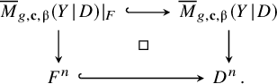
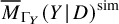
The ultimate goal of this section is to relate the above invariants to the ones of an open subset of (a deformation of) the threefold ![]() . Let us recall the main result of [Reference van Garrel, Nabijou and Schuler45] which serves as a first step towards this direction. Writing
. Let us recall the main result of [Reference van Garrel, Nabijou and Schuler45] which serves as a first step towards this direction. Writing $\unicode{x3c0} $
for the projection
$\unicode{x3c0} $
for the projection $Y\rightarrow S$
, we set
$Y\rightarrow S$
, we set ![]() and define
and define

where $\mathbf {\tilde {c}}$
is obtained from
$\mathbf {\tilde {c}}$
is obtained from $\mathbf {\hat {c}}$
by deleting the marking with tangency along
$\mathbf {\hat {c}}$
by deleting the marking with tangency along $D_2$
.
$D_2$
.
Theorem 2.2 [Reference van Garrel, Nabijou and Schuler45, Theorem A].
Suppose $D_2 \cdot D_2 \geq 0$
and
$D_2 \cdot D_2 \geq 0$
and $\unicode{x3b2} $
is so that
$\unicode{x3b2} $
is so that $D_1\cdot \unicode{x3b2} \geq 0$
and
$D_1\cdot \unicode{x3b2} \geq 0$
and $D_2 \cdot \unicode{x3b2}> 0$
. Then
$D_2 \cdot \unicode{x3b2}> 0$
. Then
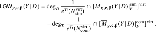
 $$ \begin{align} \sum_{g\geq 0} \hbar^{2g-2} ~\mathsf{LGW}_{g,\mathbf{\tilde{c}},\unicode{x3b2}}(Y \hspace{0.2ex}|\hspace{0.2ex} D) = \frac{(-1)^{D_2 \cdot \unicode{x3b2}+1}}{2 \sin \tfrac{(D_2 \cdot \unicode{x3b2})\hbar}{2}} \sum_{g\geq 0} \hbar^{2g-1} ~ \mathsf{LGW}_{g,\mathbf{\hat{c}},\unicode{x3b2}}(S \hspace{0.2ex}|\hspace{0.2ex} D_1+D_2)\,. \end{align} $$
2.2 Open Gromov–Witten theory
Open Gromov–Witten invariants are a delicate topic. We will work in the framework of Fang and Liu [Reference Fang and Liu14] which builds on ideas of [Reference Katz and Liu22, Reference Li and Song31]. We keep details to a minimum since at no point we will be working with open Gromov–Witten invariants directly. We refer the interested reader to [Reference Fang and Liu14, Reference Katz and Liu22] for more details.
2.2.1 Preliminaries on toric Calabi–Yau threefolds
Let X be a smooth toric Calabi–Yau threefold. We will write $\hat {T}\cong \mathbb {G}_{\mathsf {m}}^3$
for its dense torus and
$\hat {T}\cong \mathbb {G}_{\mathsf {m}}^3$
for its dense torus and $T\cong \mathbb {G}_{\mathsf {m}}^2$
for its Calabi–Yau torus. The latter is defined as the kernel
$T\cong \mathbb {G}_{\mathsf {m}}^2$
for its Calabi–Yau torus. The latter is defined as the kernel $T=\ker \unicode{x3c7} $
of the character
$T=\ker \unicode{x3c7} $
of the character $\unicode{x3c7} $
associated to the induced
$\unicode{x3c7} $
associated to the induced $\hat {T}$
-action on
$\hat {T}$
-action on $K_{X}\cong \mathcal {O}_{X}$
.
$K_{X}\cong \mathcal {O}_{X}$
.
If X can be realised as a symplectic quotient, which is the case when X is semiprojective [Reference Hausel and Sturmfels20], Aganagic and Vafa [Reference Aganagic and Vafa5] construct a certain class of Lagrangian submanifolds L in X. Relevant for us here is the fact that these Lagrangian submanifolds are invariant under the action of the maximal compact subgroup $T_{\mathbb {R}} \hookrightarrow T$
and are homeomorphic to
$T_{\mathbb {R}} \hookrightarrow T$
and are homeomorphic to $\mathbb {R}^{\!2} \times S^1$
. Moreover, these Lagrangian submanifolds intersect a unique one-dimensional torus orbit closure of X in a circle
$\mathbb {R}^{\!2} \times S^1$
. Moreover, these Lagrangian submanifolds intersect a unique one-dimensional torus orbit closure of X in a circle $S^1$
. For short, we will call a Lagrangian submanifold L of the type considered by Aganagic and Vafa an outer brane if it intersects a non-compact one-dimensional torus orbit closure.
$S^1$
. For short, we will call a Lagrangian submanifold L of the type considered by Aganagic and Vafa an outer brane if it intersects a non-compact one-dimensional torus orbit closure.
Let us write $\unicode{x3bc} $
for the moment map
$\unicode{x3bc} $
for the moment map
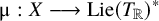 $$ \begin{align*} \unicode{x3bc} : X \longrightarrow \mathrm{Lie}(T_{\mathbb{R}})^{*} \end{align*} $$
and fix an isomorphism $\mathrm {Lie}(T_{\mathbb {R}})^{*} \cong \mathbb {R}^2$
. We call the image of the union of all one-dimensional torus orbit closures under
$\mathrm {Lie}(T_{\mathbb {R}})^{*} \cong \mathbb {R}^2$
. We call the image of the union of all one-dimensional torus orbit closures under $\unicode{x3bc} $
the toric diagram of X. It is an embedded trivalent graph since there are always three
$\unicode{x3bc} $
the toric diagram of X. It is an embedded trivalent graph since there are always three $\hat {T}$
-preserved one-dimensional strata meeting in a torus fixed point (see Figure 1). Now let L be an outer brane in X. By our earlier discussion, its image
$\hat {T}$
-preserved one-dimensional strata meeting in a torus fixed point (see Figure 1). Now let L be an outer brane in X. By our earlier discussion, its image $\unicode{x3bc} (L)$
under the moment must be a point on a non-compact edge
$\unicode{x3bc} (L)$
under the moment must be a point on a non-compact edge $\ell $
. Let us write q for the unique torus fixed point contained in
$\ell $
. Let us write q for the unique torus fixed point contained in $\ell $
and denote by
$\ell $
and denote by
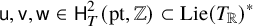 $$ \begin{align*} \mathsf{u},\mathsf{v},\mathsf{w} \in \mathsf{H}^2_{T}(\mathrm{pt},\mathbb{Z}) \subset \mathrm{Lie}(T_{\mathbb{R}})^{*} \end{align*} $$
the weights of the induced T action on the tangent spaces of three torus orbit closures at this point. Here, $\mathsf {u} = c^{T}_1(T_q \ell )$
and
$\mathsf {u} = c^{T}_1(T_q \ell )$
and $\mathsf {v}$
is chosen so that
$\mathsf {v}$
is chosen so that $\mathsf {u} \wedge \mathsf {v}\geq 0$
as indicated in Figure 1. A framing of L is the choice of an element
$\mathsf {u} \wedge \mathsf {v}\geq 0$
as indicated in Figure 1. A framing of L is the choice of an element $\mathsf {f}\in \mathsf {H}^2_{T}(\mathrm {pt},\mathbb {Z})$
satisfyingFootnote
4
$\mathsf {f}\in \mathsf {H}^2_{T}(\mathrm {pt},\mathbb {Z})$
satisfyingFootnote
4
 $$ \begin{align*} \mathsf{u} \wedge \mathsf{f} = \mathsf{u} \wedge \mathsf{v}\,. \end{align*} $$
Equivalently, we have
 $$ \begin{align} \mathsf{f} = \mathsf{v} - f \mathsf{u} \end{align} $$
for some $f\in \mathbb {Z}$
. Moreover, as an element in
$f\in \mathbb {Z}$
. Moreover, as an element in $\mathsf {H}^2_{T}(\mathrm {pt},\mathbb {Z})$
, one may view
$\mathsf {H}^2_{T}(\mathrm {pt},\mathbb {Z})$
, one may view $\mathsf {f}$
as a character
$\mathsf {f}$
as a character $T \rightarrow \mathbb {G}_{\mathsf {m}}$
. This defines a one-dimensional subtorus
$T \rightarrow \mathbb {G}_{\mathsf {m}}$
. This defines a one-dimensional subtorus ![]() which we will refer to as the framing subtorus. Finally, let us denote by
which we will refer to as the framing subtorus. Finally, let us denote by $\lvert _{\mathsf {f}=0}$
the restriction map
$\lvert _{\mathsf {f}=0}$
the restriction map
 $$ \begin{align*} \mathsf{H}_{*}^{T}(\mathrm{pt},\mathbb{Z}) \longrightarrow \mathsf{H}_{*}^{T_{\mathsf{f}}}(\mathrm{pt},\mathbb{Z}) \end{align*} $$
as this morphism essentially sets the weight $\mathsf {f}$
equal to zero.
$\mathsf {f}$
equal to zero.
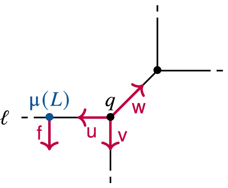
Figure 1 The image of the toric skeleton (black) of $\operatorname *{\mathrm {Tot}} \mathcal {O}_{\mathbb {P}^1}(-1) \oplus \mathcal {O}_{\mathbb {P}^1}(-1)$
with an outer brane L (blue) in framing
$\operatorname *{\mathrm {Tot}} \mathcal {O}_{\mathbb {P}^1}(-1) \oplus \mathcal {O}_{\mathbb {P}^1}(-1)$
with an outer brane L (blue) in framing $f=0$
(red) under the moment map.
$f=0$
(red) under the moment map.
Definition 2.3. A toric triple $(X,L,\mathsf {f})$
consists of
$(X,L,\mathsf {f})$
consists of
-
• a smooth semiprojective toric Calabi–Yau threefold X,
-
• an outer brane L,
-
• a framing
$\mathsf {f}$
.

Remark 2.4. To cover certain interesting cases, it will actually be necessary to relax the above definition slightly. Concretely, we would like to include the case where X is not semiprojective in our discussion as well. In this case, we replace the second point in the above definition with the choice of some non-compact one-dimensional torus orbit closure $\ell $
.
$\ell $
.
2.2.2 Open Gromov–Witten invariants
Given a toric triple $(X,L,\mathsf {f})$
and a collection
$(X,L,\mathsf {f})$
and a collection $\mathbf {c}=(c_1,\ldots ,c_n)$
of positive integers, we denote by
$\mathbf {c}=(c_1,\ldots ,c_n)$
of positive integers, we denote by
 $$ \begin{align*} \overline{M}_{g,\mathbf{c},\unicode{x3b2}^{\prime}}(X,L) \end{align*} $$
the moduli space parametrising genus g stable maps $f:(C,\partial C) \rightarrow (X,L)$
whose domain C is a Riemann surface with n labelled boundary components
$f:(C,\partial C) \rightarrow (X,L)$
whose domain C is a Riemann surface with n labelled boundary components $\partial C = \partial C_1 \sqcup \ldots \sqcup \partial C_n$
such that for all
$\partial C = \partial C_1 \sqcup \ldots \sqcup \partial C_n$
such that for all $i\in \{1,\ldots ,n\}$
,
$i\in \{1,\ldots ,n\}$
,
 $$ \begin{align*} f_{*} [\partial C_i] = c_i [S^1]\in \mathsf{H}_1(L,\mathbb{Z}) \quad\text{ and }\quad f_{*} [C] = \unicode{x3b2}^{\prime} + \textstyle{\sum_i} c_i [B] \in \mathsf{H}_2(X,L,\mathbb{Z})\,. \end{align*} $$
Here, $\unicode{x3b2} ^{\prime }$
a curve class in X and B is the unique
$\unicode{x3b2} ^{\prime }$
a curve class in X and B is the unique $T_{\mathbb {R}}$
-preserved disk stretching out from q to the circle
$T_{\mathbb {R}}$
-preserved disk stretching out from q to the circle $S^1$
in which L and
$S^1$
in which L and $\ell $
intersect. The virtual dimension of this moduli problem is zero. We refer to [Reference Katz and Liu22] for details.
$\ell $
intersect. The virtual dimension of this moduli problem is zero. We refer to [Reference Katz and Liu22] for details.
Moduli spaces parametrising stable maps with boundaries are (if they actually exist) usually notoriously hard to work with. In our case, there is, however, a way out. Since the Calabi–Yau torus $T_{\mathbb {R}}$
leaves L invariant, the
$T_{\mathbb {R}}$
leaves L invariant, the $T_{\mathbb {R}}$
-action on X lifts to an action on
$T_{\mathbb {R}}$
-action on X lifts to an action on $\overline {M}_{g,\mathbf {c},\unicode{x3b2} ^{\prime }}(X,L)$
. Then as opposed to its ambient space, the (anticipated) fixed locus
$\overline {M}_{g,\mathbf {c},\unicode{x3b2} ^{\prime }}(X,L)$
. Then as opposed to its ambient space, the (anticipated) fixed locus
 $$ \begin{align*} \overline{M}_{g,\mathbf{c},\unicode{x3b2}^{\prime}}(X,L)^{T_{\mathbb{R}}} \end{align*} $$
is a compact complex orbifold. So as in [Reference Fang and Liu14], we define open Gromov–Witten invariants via virtual localisation:
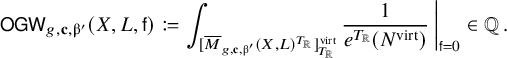
The above integral produces a rational function in the two equivariant parameters of homogenous degree zero. Only the restriction to the framing subtorus yields a rational number. This is how definition (2.4) depends on the choice of framing $\mathsf {f}$
.
$\mathsf {f}$
.
We recall a result of Fang and Liu which allows us to express open Gromov–Witten invariants of $(X,L,\mathsf {f})$
in terms of descendant invariants of X.
$(X,L,\mathsf {f})$
in terms of descendant invariants of X.
Theorem 2.5 [Reference Fang and Liu14, Proposition 3.4].
If $(X,L,\mathsf {f})$
is a toric triple, then
$(X,L,\mathsf {f})$
is a toric triple, then

where $\unicode{x3c6} $
is the T-equivariant Poincaré dual of the torus fixed point q contained in the one-dimensional torus orbit closure
$\unicode{x3c6} $
is the T-equivariant Poincaré dual of the torus fixed point q contained in the one-dimensional torus orbit closure $\ell $
intersected by L.
$\ell $
intersected by L.
Remark 2.6. In [Reference Li, Liu, Liu and Zhou30] Li, Liu, Liu and Zhou generalise the definition of open Gromov–Witten invariants to the case when X is not semiprojective. (This assumption was necessary for the construction of Aganagic–Vafa Lagrangian submanifolds.) In this case, the datum of an outer brane gets replaced by the choice of a non-compact one-dimensional torus orbit closure $\ell $
, and open Gromov–Witten invariants are defined via formal relative invariants. It is shown in [Reference Fang and Liu14, Corollary 3.3] that these invariants still satisfy Theorem 2.5.
$\ell $
, and open Gromov–Witten invariants are defined via formal relative invariants. It is shown in [Reference Fang and Liu14, Corollary 3.3] that these invariants still satisfy Theorem 2.5.
2.3 Statement of the main correspondence
Let $(S \hspace {0.2ex}|\hspace {0.2ex} D_1+D_2)$
be a two-component Looijenga pair and
$(S \hspace {0.2ex}|\hspace {0.2ex} D_1+D_2)$
be a two-component Looijenga pair and $\unicode{x3b2} $
an effective curve class in S. We demand that this data satisfies Assumption ★ which we recall means that
$\unicode{x3b2} $
an effective curve class in S. We demand that this data satisfies Assumption ★ which we recall means that
-
•
$D_i \cdot \unicode{x3b2}>0$
,
$i\in \{1,2\}$
, -
•
$D_2 \cdot D_2\geq 0$
, -
•
$(S\hspace {0.2ex}|\hspace {0.2ex} D_1)$
deforms into a pair
$(S^{\prime } \hspace {0.2ex}|\hspace {0.2ex} D_1^{\prime })$
with
$S^{\prime }$
a smooth projective toric surface and
$D_1^{\prime }$
a toric hypersurface.


Remark 2.7. By the last condition, we mean that there is a logarithmically smooth morphism of fine saturated logarithmic schemes $\mathcal {S} \rightarrow T$
with T irreducible and integral together with a line bundle
$\mathcal {S} \rightarrow T$
with T irreducible and integral together with a line bundle $\mathcal {L}$
on
$\mathcal {L}$
on $\mathcal {S}$
. Moreover, there are regular points
$\mathcal {S}$
. Moreover, there are regular points ![]() with fibres
with fibres
 $$ \begin{align*} \mathcal{S}_{t} = (S\hspace{0.2ex}|\hspace{0.2ex} D_1)\, , \qquad \mathcal{S}_{t^{\prime}} = (S^{\prime}\hspace{0.2ex}|\hspace{0.2ex} D_1^{\prime}) \end{align*} $$
on which $\mathcal {L}$
restricts to
$\mathcal {L}$
restricts to $\mathcal {L}_t = \mathcal {O}_{S}(-D_2)$
and
$\mathcal {L}_t = \mathcal {O}_{S}(-D_2)$
and $\mathcal {L}_{t'} = \unicode{x3c9} _{S^{\prime }}(D_1^{\prime })$
where
$\mathcal {L}_{t'} = \unicode{x3c9} _{S^{\prime }}(D_1^{\prime })$
where $\unicode{x3c9} _{S^{\prime }}$
is the canonical bundle on
$\unicode{x3c9} _{S^{\prime }}$
is the canonical bundle on $S^{\prime }$
.
$S^{\prime }$
.
Given $(S^{\prime } \hspace {0.2ex}|\hspace {0.2ex} D_1^{\prime })$
as above, we write
$(S^{\prime } \hspace {0.2ex}|\hspace {0.2ex} D_1^{\prime })$
as above, we write ![]() and write D for the preimage of
and write D for the preimage of $D_1^{\prime }$
under the projection
$D_1^{\prime }$
under the projection $\unicode{x3c0} : Y \rightarrow S^{\prime }$
. We remark that all compact one-dimensional torus orbit closures in Y come from the toric boundary of
$\unicode{x3c0} : Y \rightarrow S^{\prime }$
. We remark that all compact one-dimensional torus orbit closures in Y come from the toric boundary of $S^{\prime }$
embedded via the zero section
$S^{\prime }$
embedded via the zero section $S^{\prime } \hookrightarrow Y$
. This way, we may especially view
$S^{\prime } \hookrightarrow Y$
. This way, we may especially view $D_1^{\prime }$
as a toric curve in Y.
$D_1^{\prime }$
as a toric curve in Y.
Construction 2.8. To $(S \hspace {0.2ex}|\hspace {0.2ex} D_1+D_2)$
as above, we associate the toric triple
$(S \hspace {0.2ex}|\hspace {0.2ex} D_1+D_2)$
as above, we associate the toric triple $(X,L,\mathsf {f})$
, where
$(X,L,\mathsf {f})$
, where
and $L\subset X \subset Y$
is an outer brane intersecting a compact one-dimensional torus orbit closure
$L\subset X \subset Y$
is an outer brane intersecting a compact one-dimensional torus orbit closure $\ell \subset Y$
adjacent to
$\ell \subset Y$
adjacent to $D_1^{\prime }$
. The action of the Calabi–Yau torus T of X naturally extends to Y. Writing F for the fibre
$D_1^{\prime }$
. The action of the Calabi–Yau torus T of X naturally extends to Y. Writing F for the fibre $\unicode{x3c0} ^{-1}(p)$
over the point
$\unicode{x3c0} ^{-1}(p)$
over the point $p = \ell \cap D_1^{\prime }$
, we set
$p = \ell \cap D_1^{\prime }$
, we set ![]() to be the weight of the T-action on F.
to be the weight of the T-action on F.
We are now able to state our main result. For this, we fix $c_1,\ldots ,c_n> 0$
with
$c_1,\ldots ,c_n> 0$
with $\sum _i c_i = D_1 \cdot \unicode{x3b2} $
and denote by
$\sum _i c_i = D_1 \cdot \unicode{x3b2} $
and denote by $\mathbf {\hat {c}}$
the contact datum
$\mathbf {\hat {c}}$
the contact datum

along $D_1+D_2$
. We assume
$D_1+D_2$
. We assume $m\leq n$
.
$m\leq n$
.
Theorem 2.9 (Theorem 1.2).
Under Assumption ★, we have
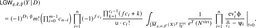
 $$ \begin{align} \sum_{g\geq 0} \hbar^{2g-2} ~ \mathsf{OGW}_{g,\mathbf{c},\unicode{x3b2}^{\prime}}(X,L,\mathsf{f}) = \frac{(-1)^{D_1 \cdot \unicode{x3b2}}}{m! \, \textstyle{\prod_{i=0}^{m-1}} c_{n-i}} ~ \frac{(-1)^{D_2 \cdot \unicode{x3b2} +1}}{2 \sin \tfrac{(D_2 \cdot \unicode{x3b2})\hbar}{2}} ~ \sum_{g\geq 0} \hbar^{2g-1} ~ \mathsf{LGW}_{g,\mathbf{\hat{c}},\unicode{x3b2}}(S \hspace{0.2ex}|\hspace{0.2ex} D_1+D_2), \end{align} $$
where $\unicode{x3b2} ^{\prime } = \unicode{x3b9} ^{*} \big (\unicode{x3b2} - (D_1 \cdot \unicode{x3b2} ) [\ell ]\big )$
and
$\unicode{x3b2} ^{\prime } = \unicode{x3b9} ^{*} \big (\unicode{x3b2} - (D_1 \cdot \unicode{x3b2} ) [\ell ]\big )$
and $\unicode{x3b9} $
is the open inclusion
$\unicode{x3b9} $
is the open inclusion $X \hookrightarrow Y$
.
$X \hookrightarrow Y$
.
See Section 5.1.2 for an extended example illustrating Construction 2.8 and an application of the above theorem.
Remark 2.10. Note that Construction 2.8 depends on the choice of which of the two torus orbit closures adjacent to $D_1$
the Lagrangian submanifold L is intersecting. Hence, a priori, one should expect the right-hand side of (2.8) to depend on this choice as well and it should come as a surprise that Theorem 2.9 actually demonstrates an independence.
$D_1$
the Lagrangian submanifold L is intersecting. Hence, a priori, one should expect the right-hand side of (2.8) to depend on this choice as well and it should come as a surprise that Theorem 2.9 actually demonstrates an independence.
Remark 2.11. If X as constructed in 2.8 turns out to be non-semiprojective, the left-hand side of equation (2.7) can still be defined as described in Remark 2.6.
Remark 2.12. Let us quickly comment on the importance of Assumption ★. The first two points guarantee that the moduli stack of relative stable maps to $(Y \hspace {0.2ex}|\hspace {0.2ex} D)$
is proper, which is required in Theorem 2.2. The last point in Assumption ★ is necessary for X to be toric, which is in turn required in the definition of open Gromov–Witten invariants we use. The condition is rather technical but allows us treat interesting cases such as the example we will discuss in Section 5.1.2.
$(Y \hspace {0.2ex}|\hspace {0.2ex} D)$
is proper, which is required in Theorem 2.2. The last point in Assumption ★ is necessary for X to be toric, which is in turn required in the definition of open Gromov–Witten invariants we use. The condition is rather technical but allows us treat interesting cases such as the example we will discuss in Section 5.1.2.
We observe that in the light of Theorem 2.2 and Theorem 2.5, it suffices to prove the following proposition in order to deduce Theorem 2.9.
Proposition 2.13. Under Assumption ★, we have
where $\unicode{x3b2} ^{\prime }=\unicode{x3b9} ^{*} (\unicode{x3b2} - (D_1 \cdot \unicode{x3b2} ) [\ell ])$
and
$\unicode{x3b2} ^{\prime }=\unicode{x3b9} ^{*} (\unicode{x3b2} - (D_1 \cdot \unicode{x3b2} ) [\ell ])$
and $\unicode{x3c6} $
is the T-equivariant Poincaré dual of the torus fixed point q in
$\unicode{x3c6} $
is the T-equivariant Poincaré dual of the torus fixed point q in $\ell \cap X$
.
$\ell \cap X$
.
We will prove this statement in two steps:
-
• In Section 3, we first establish the special case
$m=0$
(Proposition 3.1). -
• In Section 4, we prove the general case via a reduction argument (Proposition 4.1).

But before we embark on proving Proposition 2.13, let us quickly convince ourselves that the proposition indeed implies Theorem 2.9.
Proof of Theorem 2.9.
Comparing formula (2.5) and (2.8), we deduce
 $$ \begin{align*} \mathsf{OGW}_{g,\mathbf{c},\unicode{x3b2}^{\prime}}(X,L,\mathsf{f}) = \frac{(-1)^{D_1 \cdot \unicode{x3b2}}}{m! \, \textstyle{\prod_{i=0}^{m-1}} c_{n-i}} \cdot \mathsf{LGW}_{g,\mathbf{\tilde{c}},\unicode{x3b2}}(Y \hspace{0.2ex}|\hspace{0.2ex} D)\,. \end{align*} $$
Now by deformation invariance [Reference Gross and Siebert19, Theorem 0.3] (see also [Reference Mandel and Ruddat36, Appendix A]), the Gromov–Witten invariants of $(S \hspace {0.2ex}|\hspace {0.2ex} D_1)$
and
$(S \hspace {0.2ex}|\hspace {0.2ex} D_1)$
and $(S^{\prime } \hspace {0.2ex}|\hspace {0.2ex} D_1^{\prime })$
agree. In combination with Theorem 2.2, this therefore gives the identity stated in Theorem 2.9.
$(S^{\prime } \hspace {0.2ex}|\hspace {0.2ex} D_1^{\prime })$
agree. In combination with Theorem 2.2, this therefore gives the identity stated in Theorem 2.9.
3 Step I: no interior markings
This section is devoted to the proof of a special instance of Proposition 2.13.
Proposition 3.1. The statement of Proposition 2.13 holds if there are no interior markings ( $m=0$
).
$m=0$
).
We prove the proposition via virtual localisation [Reference Graber and Pandharipande16] which allows us to decompose the Gromov–Witten invariant on the left-hand side of equation (2.8) into contributions labelled by the fixed loci of a torus action on the moduli stack of relative stable maps to $(Y\hspace {0.2ex}|\hspace {0.2ex} D)$
. These loci split into two classes: the ones for which the target
$(Y\hspace {0.2ex}|\hspace {0.2ex} D)$
. These loci split into two classes: the ones for which the target $(Y\hspace {0.2ex}|\hspace {0.2ex} D)$
is generically expanded or unexpanded. A careful analysis of the latter shows that their contribution to the overall Gromov–Witten count is precisely the expression we find on the right-hand side of equation (2.8) (Proposition 3.3). It therefore remains to show the contribution of all other fixed loci vanishes. This last step is carried out in Section 3.4.
$(Y\hspace {0.2ex}|\hspace {0.2ex} D)$
is generically expanded or unexpanded. A careful analysis of the latter shows that their contribution to the overall Gromov–Witten count is precisely the expression we find on the right-hand side of equation (2.8) (Proposition 3.3). It therefore remains to show the contribution of all other fixed loci vanishes. This last step is carried out in Section 3.4.
We start with a careful analysis of the target geometry $(Y\hspace {0.2ex}|\hspace {0.2ex} D)$
where we adopt the notation introduced in Section 2.3. To unload notation throughout this section, we will assume that S is already toric and
$(Y\hspace {0.2ex}|\hspace {0.2ex} D)$
where we adopt the notation introduced in Section 2.3. To unload notation throughout this section, we will assume that S is already toric and $D_1$
is a toric hypersurface, which means we can take
$D_1$
is a toric hypersurface, which means we can take $(S^{\prime }\hspace {0.2ex}|\hspace {0.2ex} D_1^{\prime }) = (S\hspace {0.2ex}|\hspace {0.2ex} D_1)$
.
$(S^{\prime }\hspace {0.2ex}|\hspace {0.2ex} D_1^{\prime }) = (S\hspace {0.2ex}|\hspace {0.2ex} D_1)$
.
3.1 The geometric setup
The Calabi–Yau torus T of X also naturally acts on Y as both varieties share the same dense open torus. The compact one-dimensional torus orbit closures of Y are given by the irreducible components of the toric boundary of S embedded into Y by the zero section. We write $\ell \hookrightarrow Y$
for the component intersected by L. By construction,
$\ell \hookrightarrow Y$
for the component intersected by L. By construction, $\ell $
intersects
$\ell $
intersects $D_1\hookrightarrow Y$
transversely in a torus fixed point which we denote p. We write q for the second torus fixed point of
$D_1\hookrightarrow Y$
transversely in a torus fixed point which we denote p. We write q for the second torus fixed point of $\ell $
.
$\ell $
.
Figure 2 shows the image of one-dimensional torus orbit closures of Y under the moment map locally around $D_1$
. In this sketch, dashed lines correspond to non-compact orbit closures, while the dotted lines indicate that the toric boundary of
$D_1$
. In this sketch, dashed lines correspond to non-compact orbit closures, while the dotted lines indicate that the toric boundary of $S\hookrightarrow Y$
forms a circle. Moreover, the red labels represent the weights with which the torus T is acting on the tangent spaces of the respective torus orbit closures at a fixed point. The observation (see [Reference van Garrel, Nabijou and Schuler45, Lemma 2.7]) that
$S\hookrightarrow Y$
forms a circle. Moreover, the red labels represent the weights with which the torus T is acting on the tangent spaces of the respective torus orbit closures at a fixed point. The observation (see [Reference van Garrel, Nabijou and Schuler45, Lemma 2.7]) that
 $$ \begin{align} c_1^{T}(T_{p}F) = - c_1^{T}(T_{p}D_1) = \mathsf{f} \end{align} $$
will be crucial in our localisation calculation later. Moreover, we also note that the framing factor f introduced in (2.3) can be identified with the degrees
 $$ \begin{align*} f = \deg \mathcal{O}_{S}(-D_2)\big\lvert_{\ell}= -\deg N_{\ell}Y - 1\,. \end{align*} $$
The toric diagram of $X = Y \setminus D$
is obtained from the one displayed in Figure 2 by erasing the top vertical line. In this process, the divisor
$X = Y \setminus D$
is obtained from the one displayed in Figure 2 by erasing the top vertical line. In this process, the divisor $\ell $
gets decompactified, and so L is indeed an outer brane.
$\ell $
gets decompactified, and so L is indeed an outer brane.
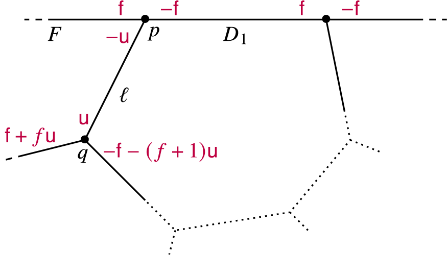
Figure 2 The image of the toric skeleton of Y under the moment map.
3.2 Initialising the localisation
Construction 2.8 involved the choice of a stratum $\ell $
the outer brane is intersecting. We now do an analogous choice by supporting the cycle whose pushforward gives the Gromov–Witten invariant
$\ell $
the outer brane is intersecting. We now do an analogous choice by supporting the cycle whose pushforward gives the Gromov–Witten invariant $\mathsf {LGW}_{g,\mathbf {c},\unicode{x3b2} }(Y \hspace {0.2ex}|\hspace {0.2ex} D)$
on a substack with evaluations constrained to the fibre
$\mathsf {LGW}_{g,\mathbf {c},\unicode{x3b2} }(Y \hspace {0.2ex}|\hspace {0.2ex} D)$
on a substack with evaluations constrained to the fibre $F=\unicode{x3c0} ^{-1}(p)$
where
$F=\unicode{x3c0} ^{-1}(p)$
where $\unicode{x3c0} $
is the projection
$\unicode{x3c0} $
is the projection $Y\rightarrow S$
:
$Y\rightarrow S$
:
Pulling back the obstruction theory along the horizontal arrow, we obtain
 $$ \begin{align*} \mathsf{LGW}_{g,\mathbf{c},\unicode{x3b2}}(Y \hspace{0.2ex}|\hspace{0.2ex} D) = \deg [\overline{M}_{g,\mathbf{c},\unicode{x3b2}}(Y \hspace{0.2ex}|\hspace{0.2ex} D)\lvert_{F}]^{\mathrm{virt}}\,. \end{align*} $$
This choice will turn out rather useful when we will calculate the invariant via virtual localisation. Regarding this, we remark that the T-action on Y lifts to an action on $\overline {M}_{g,\mathbf {c},\unicode{x3b2} }(Y \hspace {0.2ex}|\hspace {0.2ex} D)\lvert _{F}$
since D and F are both preserved by T. Especially, this also provides us with an action of the framing subtorus
$\overline {M}_{g,\mathbf {c},\unicode{x3b2} }(Y \hspace {0.2ex}|\hspace {0.2ex} D)\lvert _{F}$
since D and F are both preserved by T. Especially, this also provides us with an action of the framing subtorus $T_{\mathsf {f}}$
on the moduli stack.
$T_{\mathsf {f}}$
on the moduli stack.
Now equation (3.1) tells us that the divisor D is pointwise fixed under $T_{\mathsf {f}}$
since the restriction
$T_{\mathsf {f}}$
since the restriction $T_{\mathsf {f}}\hookrightarrow T$
effectively sets the weight
$T_{\mathsf {f}}\hookrightarrow T$
effectively sets the weight $\mathsf {f}$
equal to zero. This means we are in a situation where the analysis of Graber and Vakil [Reference Graber and Vakil17] of virtual localisation in the context of stable maps relative a smooth divisor applies. Since their analysis was carried out in the setting of relative stable maps to expanded degenerations as introduced by Li [Reference Li28, Reference Li29], we quietly pass to this modification of
$\mathsf {f}$
equal to zero. This means we are in a situation where the analysis of Graber and Vakil [Reference Graber and Vakil17] of virtual localisation in the context of stable maps relative a smooth divisor applies. Since their analysis was carried out in the setting of relative stable maps to expanded degenerations as introduced by Li [Reference Li28, Reference Li29], we quietly pass to this modification of $\overline {M}_{g,\mathbf {c},\unicode{x3b2} }(Y \hspace {0.2ex}|\hspace {0.2ex} D)$
until the end of this section without actually changing our notation. Since eventually we push all cycles forward to a point, it does not matter which birational model we choose for our moduli stack [Reference Abramovich, Marcus and Wise3]. See also [Reference Molcho and Routis40] for an analysis of torus localisation in the context of Kim’s logarithmic stable maps to expanded degenerations [Reference Kim24].
$\overline {M}_{g,\mathbf {c},\unicode{x3b2} }(Y \hspace {0.2ex}|\hspace {0.2ex} D)$
until the end of this section without actually changing our notation. Since eventually we push all cycles forward to a point, it does not matter which birational model we choose for our moduli stack [Reference Abramovich, Marcus and Wise3]. See also [Reference Molcho and Routis40] for an analysis of torus localisation in the context of Kim’s logarithmic stable maps to expanded degenerations [Reference Kim24].
Following Graber and Vakil [Reference Graber and Vakil17], we split the $T_{\mathsf {f}}$
-fixed locus
$T_{\mathsf {f}}$
-fixed locus $\overline {M}_{g,\mathbf {c},\unicode{x3b2} }(Y \hspace {0.2ex}|\hspace {0.2ex} D)^{T_{\mathsf {f}}}$
into two distinguished (not necessarily connected or irreducible) components. First, there is the simple fixed locus
$\overline {M}_{g,\mathbf {c},\unicode{x3b2} }(Y \hspace {0.2ex}|\hspace {0.2ex} D)^{T_{\mathsf {f}}}$
into two distinguished (not necessarily connected or irreducible) components. First, there is the simple fixed locus
 $$ \begin{align*} \overline{M}_{g,\mathbf{c},\unicode{x3b2}}(Y \hspace{0.2ex}|\hspace{0.2ex} D)^{\mathrm{sim}} \end{align*} $$
whose general points are stable maps with target Y. The complement of this is called composite fixed locus, and consequently, its general points correspond to maps to nontrivial expanded degenerations of $(Y \hspace {0.2ex}|\hspace {0.2ex} D)$
. We will denote this component by
$(Y \hspace {0.2ex}|\hspace {0.2ex} D)$
. We will denote this component by
 $$ \begin{align*} \overline{M}_{g,\mathbf{c},\unicode{x3b2}}(Y \hspace{0.2ex}|\hspace{0.2ex} D)^{\mathrm{com}}\,. \end{align*} $$
As we did in (3.2), we form fibre products
Then virtual localisation [Reference Graber and Pandharipande16] gives
 $$ \begin{align} \begin{aligned} \mathsf{LGW}_{g,\mathbf{c},\unicode{x3b2}}(Y \hspace{0.2ex}|\hspace{0.2ex} D) &= \deg_{T_{\mathsf{f}}} \frac{1}{e^{T_{\mathsf{f}}}(N^{\mathrm{virt}}_{\mathrm{sim}})}\cap [\overline{M}_{g,\mathbf{c},\unicode{x3b2}}(Y \hspace{0.2ex}|\hspace{0.2ex} D)\lvert_{F}^{\mathrm{sim}}]^{\mathrm{virt}}\\& \quad + \deg_{T_{\mathsf{f}}} \frac{1}{e^{T_{\mathsf{f}}}(N^{\mathrm{virt}}_{\mathrm{com}})}\cap [\overline{M}_{g,\mathbf{c},\unicode{x3b2}}(Y \hspace{0.2ex}|\hspace{0.2ex} D)\lvert_{F}^{\mathrm{com}}]^{\mathrm{virt}}\,. \end{aligned} \end{align} $$
We will inspect the contribution of the simple and composite fixed locus to the Gromov–Witten invariant individually in the next two subsections.
3.3 The simple fixed locus
Closely following [Reference Graber and Vakil17], we start with an analysis of the simple fixed locus. By definition, the image of a relative stable map $f:C\rightarrow Y$
parametrised by
$f:C\rightarrow Y$
parametrised by
 $$ \begin{align*} \overline{M}_{g,\mathbf{c},\unicode{x3b2}}(Y \hspace{0.2ex}|\hspace{0.2ex} D)\lvert_{F}^{\mathrm{sim}} \end{align*} $$
intersects D transversely (i.e., $f^{*} D = \sum _{i=1}^n c_i x_i$
as Cartier divisors where
$f^{*} D = \sum _{i=1}^n c_i x_i$
as Cartier divisors where $x_1,\ldots ,x_n$
denote the markings). If we write
$x_1,\ldots ,x_n$
denote the markings). If we write
 $$ \begin{align*} C_1,\ldots,C_n \end{align*} $$
for the irreducible components containing these markings, then since $f:C\rightarrow Y$
lies in the
$f:C\rightarrow Y$
lies in the $T_{\mathsf {f}}$
-fixed locus and by assumption none of the components
$T_{\mathsf {f}}$
-fixed locus and by assumption none of the components $C_i$
get contracted, there must be a (nontrivial) lift of the action
$C_i$
get contracted, there must be a (nontrivial) lift of the action $T_{\mathsf {f}}$
on
$T_{\mathsf {f}}$
on $C_i$
(possibly after passing to some cover of
$C_i$
(possibly after passing to some cover of $T_{\mathsf {f}}$
) making
$T_{\mathsf {f}}$
) making $f\lvert _{C_i} T_{\mathsf {f}}$
-equivariant. As a consequence, for all
$f\lvert _{C_i} T_{\mathsf {f}}$
-equivariant. As a consequence, for all $i\in \{1,\ldots ,n\}$
, both
$i\in \{1,\ldots ,n\}$
, both $C_i$
and its image under f must be rational curves. Moreover, writing
$C_i$
and its image under f must be rational curves. Moreover, writing $q_i$
for the second
$q_i$
for the second $T_{\mathsf {f}}$
-fixed point of the image rational curve,
$T_{\mathsf {f}}$
-fixed point of the image rational curve, $f\lvert _{C_i}$
is the unique degree
$f\lvert _{C_i}$
is the unique degree $c_i$
cover maximally ramified over
$c_i$
cover maximally ramified over $f(x_i)$
and
$f(x_i)$
and $q_i$
.
$q_i$
.
Now since we confined the evaluation morphisms to the fibre $F\subset Y$
, we deduce that the image of each component
$F\subset Y$
, we deduce that the image of each component $C_i$
is contained in
$C_i$
is contained in $\unicode{x3c0} ^{-1}(\ell )$
, where
$\unicode{x3c0} ^{-1}(\ell )$
, where $\unicode{x3c0} $
is the projection
$\unicode{x3c0} $
is the projection $Y\rightarrow S$
and
$Y\rightarrow S$
and $\ell $
is as in Figure 2. However, since the pullback of the line bundle
$\ell $
is as in Figure 2. However, since the pullback of the line bundle $\mathcal {O}_{S}(-D_2)$
under
$\mathcal {O}_{S}(-D_2)$
under $\unicode{x3c0} \circ f$
is negative, we deduce that f has to factor through the zero section
$\unicode{x3c0} \circ f$
is negative, we deduce that f has to factor through the zero section ${S}\hookrightarrow Y$
. Hence, the image of each irreducible component
${S}\hookrightarrow Y$
. Hence, the image of each irreducible component $C_i$
has to be the curve
$C_i$
has to be the curve $\ell $
already. This also means that
$\ell $
already. This also means that $q_i=q$
for all
$q_i=q$
for all $i\in \{1,\ldots ,n\}$
.
$i\in \{1,\ldots ,n\}$
.
Now if we write $C' \sqcup \bigsqcup _{i=1}^n C_i$
for the connected components of the partial normalisation of C along the nodes
$C' \sqcup \bigsqcup _{i=1}^n C_i$
for the connected components of the partial normalisation of C along the nodes $y_i\in C_i$
mapping to q, we observe that
$y_i\in C_i$
mapping to q, we observe that $f\lvert _{C'}$
is a genus g, class
$f\lvert _{C'}$
is a genus g, class
 $$ \begin{align*} \unicode{x3b2}^{\prime} = \unicode{x3b9}^{*} \big(\unicode{x3b2} - (D_1 \cdot \unicode{x3b2}) [\ell]\big) \end{align*} $$ $T_{\mathsf {f}}$
-fixed stable map to
$T_{\mathsf {f}}$
-fixed stable map to $X = Y \setminus D$
with markings
$X = Y \setminus D$
with markings $y_1,\ldots ,y_n$
confined to q. Hence, forming the fibre square
$y_1,\ldots ,y_n$
confined to q. Hence, forming the fibre square
we can summarise the discussion up to now as follows.
Lemma 3.2. We have
 $$ \begin{align} \overline{M}_{g,\mathbf{c},\unicode{x3b2}}(Y \hspace{0.2ex}|\hspace{0.2ex} D)\lvert_{F}^{\mathrm{sim}} = \Big[\, \overline{M}_{g,n,\unicode{x3b2}^{\prime}}(X) \lvert_{q}^{T_{\mathsf{f}}} \,\Big/\, \textstyle{\prod_{i=1}^{n}}\,\mathbb{Z}/ c_i \mathbb{Z} \,\Big]\,. \end{align} $$
Using this description of the simple fixed locus, we are now able to determine its contribution to the Gromov–Witten invariant.
Proposition 3.3. We have
where $\unicode{x3c6} $
is the
$\unicode{x3c6} $
is the $T_{\mathsf {f}}$
-equivariant Poincaré dual of q.
$T_{\mathsf {f}}$
-equivariant Poincaré dual of q.
Proof. With our characterisation (3.4) of the simple fixed locus, it remains to analyse the difference between $N^{\mathrm {virt}}_{\mathrm {sim}}$
and the virtual normal bundle
$N^{\mathrm {virt}}_{\mathrm {sim}}$
and the virtual normal bundle $N^{\mathrm {virt}}$
of the fixed locus
$N^{\mathrm {virt}}$
of the fixed locus
 $$ \begin{align*} \overline{M}_{g,n,\unicode{x3b2}^{\prime}}(X)^{T_{\mathsf{f}}} \hookrightarrow \overline{M}_{g,n,\unicode{x3b2}^{\prime}}(X)\,. \end{align*} $$
First of all, note that we get an overall factor
 $$ \begin{align*} \prod_{i=1}^n \frac{1}{c_i} \end{align*} $$
from the quotient. Moreover, partially normalising along the nodes $y_1,\ldots ,y_n$
connecting
$y_1,\ldots ,y_n$
connecting $C'$
with
$C'$
with $C_1,\ldots ,C_n$
, we see that each degree
$C_1,\ldots ,C_n$
, we see that each degree $c_i$
cover
$c_i$
cover
contributes with factors
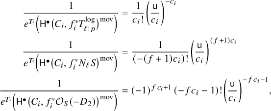 $$ \begin{align*} \frac{1}{e^{T_{\mathsf{f}}}\Big(\mathsf{H}^\bullet \big(C_i , f_i^{*} T^{\mathrm{log}}_{\ell|p} \big)^{\mathrm{mov}}\Big)} & = \frac{1}{c_i !} \bigg(\frac{\mathsf{u}}{c_i}\bigg)^{-c_i} \\ \frac{1}{e^{T_{\mathsf{f}}}\Big(\mathsf{H}^\bullet \big(C_i , f_i^{*} N_{\ell}{S} \big)^{\mathrm{mov}}\Big)} & = \frac{1}{(-(f+1)c_i)!} \bigg(\frac{\mathsf{u}}{c_i}\bigg)^{(f+1) c_i}\\ \frac{1}{e^{T_{\mathsf{f}}} \Big( \mathsf{H}^\bullet \big(C_i, f_i^{*} \mathcal{O}_{{S}}(-D_2) \big)^{\mathrm{mov}}\Big)} & = (-1)^{fc_i + 1} \, (-fc_i-1)! \bigg(\frac{\mathsf{u}}{c_i}\bigg)^{-f c_i-1}, \end{align*} $$
assuming that $f = \deg \mathcal {O}_{{S}}(-D_2)\lvert _{\ell } < 0$
. Note that if we multiply all these factors together, we indeed obtain the top line on the right-hand side of (3.5). The remaining case
$f = \deg \mathcal {O}_{{S}}(-D_2)\lvert _{\ell } < 0$
. Note that if we multiply all these factors together, we indeed obtain the top line on the right-hand side of (3.5). The remaining case $f = 0$
can be treated similarly. This is the only case left to check since
$f = 0$
can be treated similarly. This is the only case left to check since $f\leq 0$
due to our assumption that
$f\leq 0$
due to our assumption that $D_2$
is smooth and
$D_2$
is smooth and $D_2\cdot D_2 \geq 0$
. Indeed, from these assumptions, it follows that
$D_2\cdot D_2 \geq 0$
. Indeed, from these assumptions, it follows that $\ell $
intersects
$\ell $
intersects $D_2$
nonnegatively (as does any smooth curve in S), and so
$D_2$
nonnegatively (as does any smooth curve in S), and so $f = - D_2 \cdot \ell \leq 0$
.
$f = - D_2 \cdot \ell \leq 0$
.
Regarding the second line in (3.5), let us only remark that the insertions
for $i\in \{1,\ldots ,n\}$
come from smoothings of the nodes
$i\in \{1,\ldots ,n\}$
come from smoothings of the nodes $y_1,\ldots ,y_n$
.
$y_1,\ldots ,y_n$
.
3.4 Vanishing of composite contributions
We observe that the integral on the right-hand side of equation (2.8) is the result of computing the one in (3.5) via T-virtual localisation. Hence, to prove Proposition 3.1, it suffices to show the following.
Proposition 3.4. We have
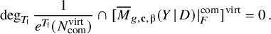 $$ \begin{align*} \deg_{T_{\mathsf{f}}} \frac{1}{e^{T_{\mathsf{f}}}(N^{\mathrm{virt}}_{\mathrm{com}})}\cap [\overline{M}_{g,\mathbf{c},\unicode{x3b2}}(Y \hspace{0.2ex}|\hspace{0.2ex} D)\lvert_{F}^{\mathrm{com}}]^{\mathrm{virt}} = 0\,. \end{align*} $$
The proof of this proposition necessitates a careful analysis of the composite fixed locus for which we will closely follow [Reference Graber and Vakil17, Section 3].
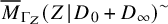
3.4.1 The setup
We first set the notation required in this section. Denote by
the projective completion of $N_{D}Y$
and write
$N_{D}Y$
and write $D_0$
and
$D_0$
and $D_\infty $
for its zero and infinity section. Note that Z is a line bundle over
$D_\infty $
for its zero and infinity section. Note that Z is a line bundle over
More precisely, we have $Z\cong \mathcal {O}_{P}(-2 f)$
where f is a fibre of
$Z\cong \mathcal {O}_{P}(-2 f)$
where f is a fibre of $P \rightarrow D_1$
.
$P \rightarrow D_1$
.
By definition, the composite fixed locus parametrises relative stable maps whose target is an expanded degeneration of $(Y \hspace {0.2ex}|\hspace {0.2ex} D)$
which is the result of gluing
$(Y \hspace {0.2ex}|\hspace {0.2ex} D)$
which is the result of gluing $(Y \hspace {0.2ex}|\hspace {0.2ex} D)$
and multiple copies of
$(Y \hspace {0.2ex}|\hspace {0.2ex} D)$
and multiple copies of $(Z \hspace {0.2ex}|\hspace {0.2ex} D_0 + D_\infty )$
to form an accordion. The composite locus decomposes into a disjoint union of components labelled by certain decorated graphs indicating how a relative stable map distributes over the expanded target.
$(Z \hspace {0.2ex}|\hspace {0.2ex} D_0 + D_\infty )$
to form an accordion. The composite locus decomposes into a disjoint union of components labelled by certain decorated graphs indicating how a relative stable map distributes over the expanded target.
Definition 3.5. A splitting type $\Gamma $
is the data of
$\Gamma $
is the data of
-
1. a bipartite graph with vertices
$V(\Gamma )$
, edges
$E(\Gamma )$
and legs
$L(\Gamma )$
; -
2. an assignment of a curve class
$\unicode{x3b2} _v$
to every vertex
$v\in V(\Gamma )$
; -
3. a genus label
$g_v\in \mathbb {Z}_{\geq 0}$
for every vertex
$v\in V(\Gamma )$
; -
4. a contact order
$d_e \in \mathbb {Z}_{> 0}$
assigned to every edge
$e\in E(\Gamma )$
; -
5. a labelling
$\{1,\ldots ,n\} \cong L(\Gamma )$
.


This data has to be compatible with $(g,\mathbf {c},\unicode{x3b2} )$
in the usual way. Vertices are separated into Y- and Z-vertices, and we will write
$(g,\mathbf {c},\unicode{x3b2} )$
in the usual way. Vertices are separated into Y- and Z-vertices, and we will write $\Gamma _Y$
and
$\Gamma _Y$
and $\Gamma _Z$
for the type of relative stable maps (with possibly disconnected domain) to
$\Gamma _Z$
for the type of relative stable maps (with possibly disconnected domain) to $(Y \hspace {0.2ex}|\hspace {0.2ex} D)$
, respectively
$(Y \hspace {0.2ex}|\hspace {0.2ex} D)$
, respectively $(Z \hspace {0.2ex}|\hspace {0.2ex} D_0+D_\infty )$
, obtained by cutting
$(Z \hspace {0.2ex}|\hspace {0.2ex} D_0+D_\infty )$
, obtained by cutting $\Gamma $
along its edges. All legs are adjacent to Z-vertices.
$\Gamma $
along its edges. All legs are adjacent to Z-vertices.
With this notation, the composite locus can be written as a union of disconnected components labelled by splitting types:
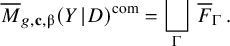 $$ \begin{align*} \overline{M}_{g,\mathbf{c},\unicode{x3b2}}(Y \hspace{0.2ex}|\hspace{0.2ex} D)^{\mathrm{com}} = \bigsqcup_{\Gamma} \, \overline{F}_{\Gamma}\,. \end{align*} $$
To characterise the component labelled by a fixed splitting type $\Gamma $
, let us denote by
$\Gamma $
, let us denote by
 $$ \begin{align*} \overline{M}_{\Gamma_Y}(Y \hspace{0.2ex}|\hspace{0.2ex} D)^{\mathrm{sim}} \end{align*} $$
the simple $T_{\mathsf {f}}$
-fixed locus of relative stable maps of type
$T_{\mathsf {f}}$
-fixed locus of relative stable maps of type $\Gamma _Y$
and write
$\Gamma _Y$
and write
 $$ \begin{align*} \overline{M}_{\Gamma_Z}(Z \hspace{0.2ex}|\hspace{0.2ex} D_0+D_\infty)^{\sim} \end{align*} $$
for the moduli stack of type $\Gamma _Z$
relative stable maps to non-rigid
$\Gamma _Z$
relative stable maps to non-rigid $(Z \hspace {0.2ex}|\hspace {0.2ex} D_0+D_\infty )$
and form a substack with constrained evaluations at marking legs
$(Z \hspace {0.2ex}|\hspace {0.2ex} D_0+D_\infty )$
and form a substack with constrained evaluations at marking legs
The two moduli stacks support evaluation morphisms to $D \cong D_0$
associated to the edges of
$D \cong D_0$
associated to the edges of $\Gamma $
. Let
$\Gamma $
. Let $\Delta $
denote the diagonal
$\Delta $
denote the diagonal $D^{E(\Gamma )} \hookrightarrow D^{E(\Gamma )}\times D^{E(\Gamma )}$
and form the fibre product
$D^{E(\Gamma )} \hookrightarrow D^{E(\Gamma )}\times D^{E(\Gamma )}$
and form the fibre product
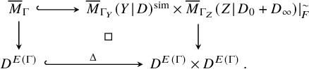
Then the connected component $\overline {F}_{\Gamma }$
of the composite fixed locus is the quotient of
$\overline {F}_{\Gamma }$
of the composite fixed locus is the quotient of $\overline {M}_{\Gamma }$
by
$\overline {M}_{\Gamma }$
by $\operatorname {\mathrm {Aut}}(d_e)$
and, moreover, by [Reference Graber and Vakil17, Lemma 3.2], the Gysin pullback
$\operatorname {\mathrm {Aut}}(d_e)$
and, moreover, by [Reference Graber and Vakil17, Lemma 3.2], the Gysin pullback
pushes forward to $[\overline {F}_{\Gamma }]^{\mathrm {virt}}$
under the quotient morphism. This means we get
$[\overline {F}_{\Gamma }]^{\mathrm {virt}}$
under the quotient morphism. This means we get
 $$ \begin{align} \deg_{T_{\mathsf{f}}} \frac{1}{e^{T_{\mathsf{f}}}(N^{\mathrm{virt}}_{\mathrm{com}})}\cap [\overline{M}_{g,\mathbf{c},\unicode{x3b2}}(Y \hspace{0.2ex}|\hspace{0.2ex} D)\lvert_{F}^{\mathrm{com}}]^{\mathrm{virt}}_{T_{\mathsf{f}}} = \sum_{\Gamma} \frac{1}{|\operatorname{\mathrm{Aut}}(d_e)|}~ \deg_{T_{\mathsf{f}}} \frac{1}{e^{T_{\mathsf{f}}}(N^{\mathrm{virt}}_{\Gamma})}\cap [\overline{M}_{\Gamma}]^{\mathrm{virt}}\,. \end{align} $$
3.4.2 First vanishing: restricted curve classes
To prove Proposition 3.4, we will show that each term in the sum (3.9) vanishes in several steps. We first recall a lemma from [Reference van Garrel, Nabijou and Schuler45].
Lemma 3.6 [Reference van Garrel, Nabijou and Schuler45, Section 2.3.3].
If there is a Z-vertex $v\in V(\Gamma )$
such that
$v\in V(\Gamma )$
such that $\unicode{x3b2} _v$
is not a multiple of a fibre of
$\unicode{x3b2} _v$
is not a multiple of a fibre of $P\rightarrow D_1$
, then
$P\rightarrow D_1$
, then
 $$ \begin{align} \deg_{T_{\mathsf{f}}} \frac{1}{e^{T_{\mathsf{f}}}(N^{\mathrm{virt}}_{\Gamma})}\cap [\overline{M}_{\Gamma}]^{\mathrm{virt}} = 0\,. \end{align} $$
Remark 3.7. The above lemma was proven in [Reference van Garrel, Nabijou and Schuler45] under the assumption that $D_1\cdot \unicode{x3b2} = 0$
but, it is straightforward to generalise the proof to the case at hand where
$D_1\cdot \unicode{x3b2} = 0$
but, it is straightforward to generalise the proof to the case at hand where $D_1\cdot \unicode{x3b2}>0$
. The key observation is that after localising the left-hand side of (3.10) with respect to T, one can identify a trivial factor in the obstruction bundle guaranteeing the vanishing.
$D_1\cdot \unicode{x3b2}>0$
. The key observation is that after localising the left-hand side of (3.10) with respect to T, one can identify a trivial factor in the obstruction bundle guaranteeing the vanishing.
3.4.3 Second vanishing: star shaped graphs
From now on, we may assume that every Z-vertex v is decorated with curve class $\unicode{x3b2} _v$
which is a multiple of a fibre of
$\unicode{x3b2} _v$
which is a multiple of a fibre of $P\rightarrow D_1$
.
$P\rightarrow D_1$
.
The following results are inspired by vanishing arguments appearing in the localisation calculations [Reference Liu and Yu32, Reference Li, Liu, Liu and Zhou30, Reference Liu, Liu and Zhou33]. We will present more geometric versions of these arguments here.
Lemma 3.8. Unless every vertex in $\Gamma _Z$
carries exactly one leg, we have
$\Gamma _Z$
carries exactly one leg, we have
 $$ \begin{align*} [\overline{M}_{\Gamma_Z}(Z \hspace{0.2ex}|\hspace{0.2ex} D_0+D_\infty)\lvert_{F}^{\sim}]^{\mathrm{virt}} = 0\,. \end{align*} $$
Proof. Clearly, every Z-vertex v has to have at least one leg for the moduli stack to be nonempty since $D_\infty \cdot \unicode{x3b2} _v>0$
. So suppose there is some vertex with at least two legs. Since the curve class carried by this vertex is a fibre class and the restriction of the line bundle
$D_\infty \cdot \unicode{x3b2} _v>0$
. So suppose there is some vertex with at least two legs. Since the curve class carried by this vertex is a fibre class and the restriction of the line bundle $Z\rightarrow P$
to a fibre trivialises, the product of the evaluation morphisms of these two markings factors through the diagonal
$Z\rightarrow P$
to a fibre trivialises, the product of the evaluation morphisms of these two markings factors through the diagonal $D_\infty \rightarrow D_\infty ^2$
. Hence, we have the following commuting diagram with Cartesian squares:
$D_\infty \rightarrow D_\infty ^2$
. Hence, we have the following commuting diagram with Cartesian squares:
Note that the excess intersection bundle
 $$ \begin{align*} E = f^{*} N_{F^{n}} D_\infty^{n} \big/ N_{F^{n-1}} D_\infty^{n-1} \end{align*} $$
is trivial as is every vector bundle on $F^{n-1} \cong \mathbb {A}^{\! n-1}$
. Moreover, note that since
$F^{n-1} \cong \mathbb {A}^{\! n-1}$
. Moreover, note that since $T_{\mathsf {f}}$
is acting trivially on
$T_{\mathsf {f}}$
is acting trivially on $D_\infty $
and F, this bundle is also
$D_\infty $
and F, this bundle is also $T_{\mathsf {f}}$
-equivariantly trivial. Therefore, by the excess intersection formula [Reference Fulton15, Theorem 6.3], we have
$T_{\mathsf {f}}$
-equivariantly trivial. Therefore, by the excess intersection formula [Reference Fulton15, Theorem 6.3], we have
 $$ \begin{align*} [\overline{M}_{\Gamma_Z}(Z \hspace{0.2ex}|\hspace{0.2ex} D_0+D_\infty)\lvert_{F}^{\sim}]^{\mathrm{virt}} {\kern-1pt}= {\kern-1pt}\unicode{x3b7}^! [\overline{M}_{\Gamma_Z}(Z \hspace{0.2ex}|\hspace{0.2ex} D_0+D_\infty)^{\sim}]^{\mathrm{virt}} {\kern-1pt}={\kern-1pt} c_1^{T_{\mathsf{f}}} (g^{*} E) \cap \overline{\unicode{x3b7}}^![\overline{M}_{\Gamma_Z}(Z \hspace{0.2ex}|\hspace{0.2ex} D_0+D_\infty)^{\sim}]^{\mathrm{virt}} {\kern-1pt}={\kern-1pt} 0. \end{align*} $$
As another consequence of our assumption that all curve classes of Z-vertices are multiples of fibre classes, the evaluation morphism associated to edges
 $$ \begin{align*} \overline{M}_{\Gamma_Z}(Z \hspace{0.2ex}|\hspace{0.2ex} D_0+D_\infty)\lvert_{F}^{\sim} \longrightarrow D_0^{E(\Gamma)} \end{align*} $$
factors through $F^{E(\Gamma )} \hookrightarrow D_0^{E(\Gamma )}$
. If we combine this with the fact that the evaluation morphism
$F^{E(\Gamma )} \hookrightarrow D_0^{E(\Gamma )}$
. If we combine this with the fact that the evaluation morphism
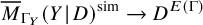 $$ \begin{align*} \overline{M}_{\Gamma_Y}(Y \hspace{0.2ex}|\hspace{0.2ex} D)^{\mathrm{sim}} \rightarrow D^{E(\Gamma)} \end{align*} $$
factors through $D^{E(\Gamma )}_1 \hookrightarrow D^{E(\Gamma )}$
we may restrict the evaluations to the intersection point
$D^{E(\Gamma )}_1 \hookrightarrow D^{E(\Gamma )}$
we may restrict the evaluations to the intersection point $p = F \cap D_1$
. We get the following commuting diagram with Cartesian squares:
$p = F \cap D_1$
. We get the following commuting diagram with Cartesian squares:
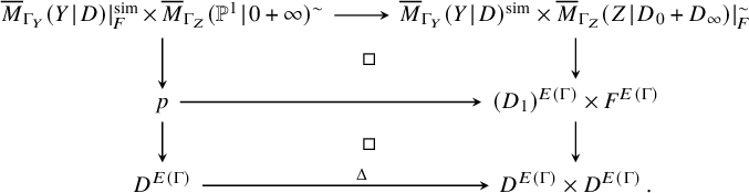
Especially, note that we have a fibre square
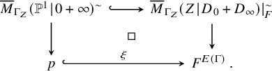
First, we record the following vanishing.
Lemma 3.9. We have $[\overline {M}_{\Gamma }]^{\mathrm {virt}} = 0$
unless every Z-vertex has a single adjacent edge.
$[\overline {M}_{\Gamma }]^{\mathrm {virt}} = 0$
unless every Z-vertex has a single adjacent edge.
Proof. The lemma can be proven with an argument similar to the one in the proof of Lemma 3.8 using diagram (3.11). We leave this to the reader.
Moreover, comparing our definition of $\overline {M}_{\Gamma }$
in (3.8) with diagram (3.11), we learn that
$\overline {M}_{\Gamma }$
in (3.8) with diagram (3.11), we learn that
 $$ \begin{align*} \overline{M}_{\Gamma} \cong \overline{M}_{\Gamma_Y}(Y \hspace{0.2ex}|\hspace{0.2ex} D)\lvert_{F}^{\mathrm{sim}}\,\times\, \overline{M}_{\Gamma_Z}(\mathbb{P}^1 \hspace{0.2ex}|\hspace{0.2ex} 0+\infty)^{\sim} \,. \end{align*} $$
On the level of virtual fundamental classes, we find the following identity.
Lemma 3.10. If there is a Z-vertex v with $g_v>0$
, the cycle
$g_v>0$
, the cycle $[\overline {M}_{\Gamma }]^{\mathrm {virt}}$
vanishes. Otherwise, the cycle equates to
$[\overline {M}_{\Gamma }]^{\mathrm {virt}}$
vanishes. Otherwise, the cycle equates to
 $$ \begin{align*} [\overline{M}_{\Gamma_Y}(Y \hspace{0.2ex}|\hspace{0.2ex} D)^{\mathrm{sim}}\lvert_{F}]^{\mathrm{virt}} \times [\overline{M}_{\Gamma_Z}(\mathbb{P}^1 \hspace{0.2ex}|\hspace{0.2ex} 0+\infty)^{\sim}]^{\mathrm{virt}}\,. \end{align*} $$
Proof. Let $\xi $
be as in (3.12). Then since all squares in (3.11) are Cartesian, we have
$\xi $
be as in (3.12). Then since all squares in (3.11) are Cartesian, we have
 $$ \begin{align*} [\overline{M}_{\Gamma}]^{\mathrm{virt}} & = \Delta^! \big( [\overline{M}_{\Gamma_Y}(Y \hspace{0.2ex}|\hspace{0.2ex} D)^{\mathrm{sim}}]^{\mathrm{virt}} \times [\overline{M}_{\Gamma_Z}(Z \hspace{0.2ex}|\hspace{0.2ex} D_0+D_\infty)\lvert_{F}^{\sim}]^{\mathrm{virt}}\big) \\[0.3em] & = [\overline{M}_{\Gamma_Y}(Y \hspace{0.2ex}|\hspace{0.2ex} D)\lvert_{F}^{\mathrm{sim}}]^{\mathrm{virt}} \times \xi^![\overline{M}_{\Gamma_Z}(Z \hspace{0.2ex}|\hspace{0.2ex} D_0+D_\infty)\lvert_{F}^{\sim}]^{\mathrm{virt}} \end{align*} $$
by [Reference Fulton15, Theorem 6.2 (c)]. Comparing the usual perfect obstruction theory of $\overline {M}_{\Gamma _Z}(\mathbb {P}^1 \hspace {0.2ex}|\hspace {0.2ex} 0+\infty )^{\sim }$
with the one pulled back from
$\overline {M}_{\Gamma _Z}(\mathbb {P}^1 \hspace {0.2ex}|\hspace {0.2ex} 0+\infty )^{\sim }$
with the one pulled back from $\overline {M}_{\Gamma _Z}(Z \hspace {0.2ex}|\hspace {0.2ex} D_0+D_\infty )\lvert _{F}^{\sim }$
, we find
$\overline {M}_{\Gamma _Z}(Z \hspace {0.2ex}|\hspace {0.2ex} D_0+D_\infty )\lvert _{F}^{\sim }$
, we find
where $\unicode{x3bb} _{\mathrm {top}}$
is the top Chern class of the Hodge bundle. The statement of the lemma then follows from the fact that
$\unicode{x3bb} _{\mathrm {top}}$
is the top Chern class of the Hodge bundle. The statement of the lemma then follows from the fact that $\unicode{x3bb} _{\mathrm {top}}^2 = 0$
if any of the vertices in
$\unicode{x3bb} _{\mathrm {top}}^2 = 0$
if any of the vertices in $\Gamma _Z$
carries a nonzero genus label and
$\Gamma _Z$
carries a nonzero genus label and $\unicode{x3bb} _{\mathrm {top}}^2 = 1$
otherwise.
$\unicode{x3bb} _{\mathrm {top}}^2 = 1$
otherwise.
3.4.4 Final vanishing
Having proven Lemmas 3.8–3.10, we are finally able to deduce Proposition 3.4.
Proof of Proposition 3.4.
According to Lemma 3.8 and 3.9, the only splitting types $\Gamma $
whose associated summand on the left-hand side of (3.9) may be nonzero consist of Z-vertices with exactly one adjacent edge and leg. Moreover, by Lemma 3.10, every such vertex has to carry a vanishing genus label. Therefore, the virtual dimension of
$\Gamma $
whose associated summand on the left-hand side of (3.9) may be nonzero consist of Z-vertices with exactly one adjacent edge and leg. Moreover, by Lemma 3.10, every such vertex has to carry a vanishing genus label. Therefore, the virtual dimension of $\overline {M}_{\Gamma _Z}(\mathbb {P}^1 \hspace {0.2ex}|\hspace {0.2ex} 0+\infty )^{\sim }$
is
$\overline {M}_{\Gamma _Z}(\mathbb {P}^1 \hspace {0.2ex}|\hspace {0.2ex} 0+\infty )^{\sim }$
is
 $$ \begin{align*} \sum_{v\in V(\Gamma_Z)} (2g_v-2) + |E(\Gamma)| + |L(\Gamma)| - 1 = -1, \end{align*} $$
and so the cycle $[\overline {M}_{\Gamma }]^{\mathrm {virt}}$
vanishes by Lemma 3.10.
$[\overline {M}_{\Gamma }]^{\mathrm {virt}}$
vanishes by Lemma 3.10.
4 Step II: reducing interior to contact insertions
4.1 The comparison statement
Throughout this section, we will assume that $(S \hspace {0.2ex}|\hspace {0.2ex} D_1+D_2)$
is a logarithmic Calabi–Yau surface with boundary the union of two transversally intersecting smooth irreducible curves
$(S \hspace {0.2ex}|\hspace {0.2ex} D_1+D_2)$
is a logarithmic Calabi–Yau surface with boundary the union of two transversally intersecting smooth irreducible curves $D_1,D_2$
. Moreover, we fix an effective curve class
$D_1,D_2$
. Moreover, we fix an effective curve class $\unicode{x3b2} $
in S and assume
$\unicode{x3b2} $
in S and assume
-
•
$D_i \cdot \unicode{x3b2}>0$
,
$i\in \{1,2\}$
, -
•
$D_2 \cdot D_2\geq 0$
.


Especially, in this section, we do not necessarily assume $(S\hspace {0.2ex}|\hspace {0.2ex} D_1)$
to deform to a toric pair. We set
$(S\hspace {0.2ex}|\hspace {0.2ex} D_1)$
to deform to a toric pair. We set ![]() and write D for the preimage of
and write D for the preimage of $D_1$
under the projection morphism.
$D_1$
under the projection morphism.
As before, we fix a contact datum $\mathbf {c}=(c_1,\ldots ,c_n)$
with D where
$\mathbf {c}=(c_1,\ldots ,c_n)$
with D where $c_i>0$
for all
$c_i>0$
for all $i\in \{1,\ldots ,n\}$
. We set
$i\in \{1,\ldots ,n\}$
. We set
 $$ \begin{align} \mathsf{LGW}_{g,\mathbf{c},\unicode{x3b2}}(Y \hspace{0.2ex}|\hspace{0.2ex} D) = \int_{[\overline{M}_{g,\mathbf{c},\unicode{x3b2}}(Y \hspace{0.2ex}|\hspace{0.2ex} D)]^{\mathrm{virt}}} \prod_{j=1}^{n} \mathrm{ev}_j^{*}\big(\unicode{x3c0}^{*}\big[\mathrm{pt}_{D_1}\big]\big)\,. \end{align} $$
Now denote by
 $$ \begin{align*} \mathbf{\tilde{c}}=(0,\ldots,0,c_1,\ldots,c_n) \end{align*} $$
the result of adding $m\leq n$
interior markings. Similarly to (4.1), we define
$m\leq n$
interior markings. Similarly to (4.1), we define $\mathsf {LGW}_{g,\mathbf {\tilde {c}},\unicode{x3b2} }(Y \hspace {0.2ex}|\hspace {0.2ex} D)\in \mathbb {Q}$
by imposing point conditions at the first n markings as in (2.1). Note that this especially means that there is a point condition at all m interior markings. We have the following comparison statement which reduces computations to the case without any interior markings.
$\mathsf {LGW}_{g,\mathbf {\tilde {c}},\unicode{x3b2} }(Y \hspace {0.2ex}|\hspace {0.2ex} D)\in \mathbb {Q}$
by imposing point conditions at the first n markings as in (2.1). Note that this especially means that there is a point condition at all m interior markings. We have the following comparison statement which reduces computations to the case without any interior markings.
Proposition 4.1. We have
 $$ \begin{align} \mathsf{LGW}_{g,\mathbf{\tilde{c}},\unicode{x3b2}}(Y \hspace{0.2ex}|\hspace{0.2ex} D) = m! \left( \textstyle{\prod_{i=0}^{m-1}}c_{n-i}\right) \cdot \mathsf{LGW}_{g,\mathbf{c},\unicode{x3b2}}(Y \hspace{0.2ex}|\hspace{0.2ex} D)\,. \end{align} $$
Together with the special case $m=0$
of Proposition 2.13, which we have already proven in the last section, the above reduction result implies the general case
$m=0$
of Proposition 2.13, which we have already proven in the last section, the above reduction result implies the general case $m\geq 0$
of Proposition 2.13 as well. The rest of this section is hence dedicated to the proof of Proposition 4.1.
$m\geq 0$
of Proposition 2.13 as well. The rest of this section is hence dedicated to the proof of Proposition 4.1.
4.2 Degeneration
To prove the main result of this section, we will use a degeneration argument similar to [Reference van Garrel, Graber and Ruddat44]. Since by now this approach has become a well-established technique [Reference Tseng and You43, Reference Battistella, Nabijou, Tseng and You6, Reference van Garrel, Nabijou and Schuler45, Reference Rabano, Manolache and Shafi42, Reference Bousseau, Fan, Guo and Wu8], we economise on details.
Recall the definition of the line bundle $Z\rightarrow P$
from equation (3.6) and (3.7) (where we identify
$Z\rightarrow P$
from equation (3.6) and (3.7) (where we identify $S=S^{\prime }$
). We defined Z to be the projective completion of
$S=S^{\prime }$
). We defined Z to be the projective completion of $N_D Y$
whose zero and infinity section we denote by
$N_D Y$
whose zero and infinity section we denote by $D_0$
and
$D_0$
and $D_{\infty }$
, respectively. Let us consider the degeneration to the normal cone of D in Y:
$D_{\infty }$
, respectively. Let us consider the degeneration to the normal cone of D in Y:
 $$ \begin{align*} \mathcal{Y} \longrightarrow \mathbb{A}^{\! 1}\,. \end{align*} $$ $\mathcal {Y}$
is a line bundle over the degeneration to the normal cone of
$\mathcal {Y}$
is a line bundle over the degeneration to the normal cone of $D_1$
in S. While the general fibre of
$D_1$
in S. While the general fibre of $\mathcal {Y}$
is Y, the special fibre
$\mathcal {Y}$
is Y, the special fibre $\mathcal {Y}_0 = Y \sqcup _D Z$
is the result of gluing Y along D to Z along the zero section
$\mathcal {Y}_0 = Y \sqcup _D Z$
is the result of gluing Y along D to Z along the zero section $D_0$
. Now let us write
$D_0$
. Now let us write $\mathcal {D}$
for the closure of
$\mathcal {D}$
for the closure of $D\times (\mathbb {A}^{\! 1} - \{0\})$
in
$D\times (\mathbb {A}^{\! 1} - \{0\})$
in $\mathcal {Y}$
and equip
$\mathcal {Y}$
and equip $\mathcal {Y}$
with the divisorial logarithmic structure with respect to
$\mathcal {Y}$
with the divisorial logarithmic structure with respect to $Y+Z+\mathcal {D}$
. The resulting logarithmic scheme has general fibre
$Y+Z+\mathcal {D}$
. The resulting logarithmic scheme has general fibre $(Y \hspace {0.2ex}|\hspace {0.2ex} D)$
, and its special fibre is obtained by gluing
$(Y \hspace {0.2ex}|\hspace {0.2ex} D)$
, and its special fibre is obtained by gluing
 $$ \begin{align*} (Y \hspace{0.2ex}|\hspace{0.2ex} D) \qquad \text{and} \qquad (Z \hspace{0.2ex}|\hspace{0.2ex} D_0+D_\infty)\,. \end{align*} $$
Finally, for F a fibre of $D\rightarrow D_1$
, we denote by
$D\rightarrow D_1$
, we denote by $\mathcal {F}$
the closure of
$\mathcal {F}$
the closure of $F \times (\mathbb {A}^{\! 1}-\{0\})$
in
$F \times (\mathbb {A}^{\! 1}-\{0\})$
in $\mathcal {Y}$
. The intersection
$\mathcal {Y}$
. The intersection $\mathcal {F}_0$
of
$\mathcal {F}_0$
of $\mathcal {F}$
with the special fibre
$\mathcal {F}$
with the special fibre $\mathcal {Y}_0$
is a fibre of
$\mathcal {Y}_0$
is a fibre of $D_\infty \rightarrow D_1$
.
$D_\infty \rightarrow D_1$
.
4.3 Decomposition
Composition with the blowup morphism $\mathcal {Y} \rightarrow Y\times \mathbb {A}^{\! 1}$
produces a pushforward
$\mathcal {Y} \rightarrow Y\times \mathbb {A}^{\! 1}$
produces a pushforward
 $$ \begin{align*} \unicode{x3c1} : \overline{M}_{g,\mathbf{\tilde{c}},\unicode{x3b2}}(\mathcal{Y}_0) \longrightarrow \overline{M}_{g,\mathbf{\tilde{c}},\unicode{x3b2}}(Y \hspace{0.2ex}|\hspace{0.2ex} D), \end{align*} $$
and by the conservation of number principle, we have
where we introduced the fibre products
and pulled back the respective virtual fundamental classes along horizontal arrows. The pushforward of the left-hand side of (4.3) to $\overline {M}_{g,\mathbf {\tilde {c}},\unicode{x3b2} }(Y \hspace {0.2ex}|\hspace {0.2ex} D)$
gives
$\overline {M}_{g,\mathbf {\tilde {c}},\unicode{x3b2} }(Y \hspace {0.2ex}|\hspace {0.2ex} D)$
gives
 $$ \begin{align*} \Pi_{i=1}^{n} \mathrm{ev}_i^{*}\big(\unicode{x3c0}^{*}\big[\mathrm{pt}_{S}\big]\big) \cdot \Pi_{j=m+1}^{n} \mathrm{ev}_j^{*}\big(\unicode{x3c0}^{*}\big[\mathrm{pt}_{D_1}\big]\big) \cap [\overline{M}_{g,\mathbf{\tilde{c}},\unicode{x3b2}}(Y \hspace{0.2ex}|\hspace{0.2ex} D)]^{\mathrm{virt}}, \end{align*} $$
and so pushing forward to a point returns the Gromov–Witten invariant we are after:
 $$ \begin{align*} \mathsf{LGW}_{g,\mathbf{\tilde{c}},\unicode{x3b2}}(Y \hspace{0.2ex}|\hspace{0.2ex} D)\,. \end{align*} $$
We combine this with the decomposition formula [Reference Abramovich, Chen, Gross and Siebert2, Theorem 5.4]
where $\unicode{x3b9} $
denotes the inclusion
$\unicode{x3b9} $
denotes the inclusion
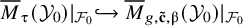 $$ \begin{align*} \overline{M}_{\unicode{x3c4}}(\mathcal{Y}_0)\lvert_{\mathcal{F}_0} \hookrightarrow \overline{M}_{g,\mathbf{\tilde{c}},\unicode{x3b2}}(\mathcal{Y}_0)\lvert_{\mathcal{F}_0} \end{align*} $$
and the sum runs over all rigid tropical types $\unicode{x3c4} $
of tropical maps to the polyhedral complex
$\unicode{x3c4} $
of tropical maps to the polyhedral complex
which is the fibre over $1\in \mathbb {R}_{\geq 0}$
of the tropicalisation
$1\in \mathbb {R}_{\geq 0}$
of the tropicalisation $\Sigma (\mathcal {Y}) \rightarrow \Sigma (\mathbb {A}^{\! 1}) = \mathbb {R}_{\geq 0}$
.
$\Sigma (\mathcal {Y}) \rightarrow \Sigma (\mathbb {A}^{\! 1}) = \mathbb {R}_{\geq 0}$
.
By the discussion in [Reference Abramovich, Chen, Gross and Siebert2, Section 5.1], $\unicode{x3c4} $
can only be rigid if all vertices of the underlying graph map to either one of the vertices
$\unicode{x3c4} $
can only be rigid if all vertices of the underlying graph map to either one of the vertices $\unicode{x3c3} _X$
or
$\unicode{x3c3} _X$
or $\unicode{x3c3} _Z$
. Hence,
$\unicode{x3c3} _Z$
. Hence, $\unicode{x3c4} $
is uniquely reconstructed from the data of its underlying decorated bipartite graph which is exactly the data of a splitting type as introduced in Definition 3.5. Hence, to be closer to the notation used in Section 3.4, let us write
$\unicode{x3c4} $
is uniquely reconstructed from the data of its underlying decorated bipartite graph which is exactly the data of a splitting type as introduced in Definition 3.5. Hence, to be closer to the notation used in Section 3.4, let us write $\Gamma $
for the splitting type underlying
$\Gamma $
for the splitting type underlying $\unicode{x3c4} $
and
$\unicode{x3c4} $
and $\Gamma _Y$
,
$\Gamma _Y$
, $\Gamma _Z$
for the type of stable logarithmic maps to
$\Gamma _Z$
for the type of stable logarithmic maps to $(Y \hspace {0.2ex}|\hspace {0.2ex} D)$
, respectively
$(Y \hspace {0.2ex}|\hspace {0.2ex} D)$
, respectively $(Z \hspace {0.2ex}|\hspace {0.2ex} D_0+D_\infty )$
, obtained by cutting
$(Z \hspace {0.2ex}|\hspace {0.2ex} D_0+D_\infty )$
, obtained by cutting $\Gamma $
along edges.
$\Gamma $
along edges.
We remark that only such rigid tropical types can contribute nontrivially to the sum (4.4) for which all marking legs are attached to a Z-vertex. Indeed, contact markings necessarily have to be adjacent to a Z-vertex, and if an interior marking is carried by a Y-vertex, then $\overline {M}_{\unicode{x3c4} }(\mathcal {Y}_0)\lvert _{\mathcal {F}_0}$
is empty (where we crucially use our assumption that
$\overline {M}_{\unicode{x3c4} }(\mathcal {Y}_0)\lvert _{\mathcal {F}_0}$
is empty (where we crucially use our assumption that $m\leq n$
). Moreover, the factor
$m\leq n$
). Moreover, the factor $m_{\unicode{x3c4} }$
in the decomposition formula (4.4) equates to
$m_{\unicode{x3c4} }$
in the decomposition formula (4.4) equates to $\mathrm {lcm}(d_e)$
, where
$\mathrm {lcm}(d_e)$
, where $d_e$
denotes contact order of an edge e.
$d_e$
denotes contact order of an edge e.
Since we are in the special setting where $\Sigma $
is of dimension one, the discussion in [Reference Gross18, Section 7] applies. There is a morphism
$\Sigma $
is of dimension one, the discussion in [Reference Gross18, Section 7] applies. There is a morphism $\unicode{x3bd} $
with target the fibre product
$\unicode{x3bd} $
with target the fibre product
which is finite and satisfies
There is a gluing morphism $\unicode{x3b8} : \overline {M}_\Gamma \rightarrow \overline {M}_{g,m+n,\unicode{x3b2} }(Y)$
such that
$\unicode{x3b8} : \overline {M}_\Gamma \rightarrow \overline {M}_{g,m+n,\unicode{x3b2} }(Y)$
such that
commutes where $\unicode{x3b6} $
denotes the forgetful morphism
$\unicode{x3b6} $
denotes the forgetful morphism
 $$ \begin{align*} \unicode{x3b6} : \overline{M}_{g,\mathbf{\tilde{c}},\unicode{x3b2}}(Y \hspace{0.2ex}|\hspace{0.2ex} D)\lvert_{F} \longrightarrow \overline{M}_{g,m+n,\unicode{x3b2}}(Y)\,. \end{align*} $$
To summarize the discussion so far, we combine equation (4.4) and (4.6) and use the fact that diagram (4.7) commutes to deduce
where we introduced the notation
4.4 Vanishing
In this section, we will argue that for most splitting types $\Gamma $
the cycle
$\Gamma $
the cycle $[\overline {M}_\Gamma ]^{\mathrm {virt}}$
vanishes. We note that our setup is almost the same as in Section 3.4. The only notable differences are as follows.
$[\overline {M}_\Gamma ]^{\mathrm {virt}}$
vanishes. We note that our setup is almost the same as in Section 3.4. The only notable differences are as follows.
-
•
$\overline {M}_{\Gamma _Y}(Y \hspace {0.2ex}|\hspace {0.2ex} D)$
parametrise logarithmic stable maps to
$(Y \hspace {0.2ex}|\hspace {0.2ex} D)$
. In Section 3.4, we considered the simple fixed locus of this moduli stack under some torus action. -
•
$\overline {M}_{\Gamma _Z}(Z \hspace {0.2ex}|\hspace {0.2ex} D_0 + D_\infty )$
parametrises logarithmic stable maps to
$(Z \hspace {0.2ex}|\hspace {0.2ex} D_0 + D_\infty )$
, while in Section 3.4, the target was non-rigid
$(Z \hspace {0.2ex}|\hspace {0.2ex} D_0 + D_\infty )$
. -
•
$\Gamma _Z$
contains interior markings.


We note that all arguments in Section 3.4 are essentially insensitive to first two differences, which allows us to prove the vanishing of $[\overline {M}_\Gamma ]^{\mathrm {virt}}$
in similar steps. Only the third point requires some attention.
$[\overline {M}_\Gamma ]^{\mathrm {virt}}$
in similar steps. Only the third point requires some attention.
4.4.1 First vanishing: fibre classes
We start with the analogue of Lemma 3.6.
Lemma 4.2. We have $[\overline {M}_{\Gamma _Z}(Z \hspace {0.2ex}|\hspace {0.2ex} D_0 + D_\infty )\lvert _{\mathcal {F}_0}]^{\mathrm {virt}}=0$
unless
$[\overline {M}_{\Gamma _Z}(Z \hspace {0.2ex}|\hspace {0.2ex} D_0 + D_\infty )\lvert _{\mathcal {F}_0}]^{\mathrm {virt}}=0$
unless $\Gamma _Z$
only consists of vertices decorated with a curve class which is a multiple of a fibre class.
$\Gamma _Z$
only consists of vertices decorated with a curve class which is a multiple of a fibre class.
Proof. Let us write $\unicode{x3b2} _Z$
for the overall curve class carried by
$\unicode{x3b2} _Z$
for the overall curve class carried by $\Gamma _Z$
and suppose its projection
$\Gamma _Z$
and suppose its projection $p_{*} \unicode{x3b2} _Z$
along the morphism
$p_{*} \unicode{x3b2} _Z$
along the morphism $p:P\rightarrow D_1$
is nonzero. In other words we assume
$p:P\rightarrow D_1$
is nonzero. In other words we assume $p_{*} \unicode{x3b2} _Z = d[D_1]$
for some
$p_{*} \unicode{x3b2} _Z = d[D_1]$
for some $d>0$
. We claim that in this case,
$d>0$
. We claim that in this case,
 $$ \begin{align*} [\overline{M}_{\Gamma_Z}(Z \hspace{0.2ex}|\hspace{0.2ex} D_0 + D_\infty)]^{\mathrm{virt}}=0\,. \end{align*} $$
To prove this, we use an argument from [Reference van Garrel, Graber and Ruddat44, Section 4]. Set $k=m+n+|E(\Gamma )|$
and consider the morphism
$k=m+n+|E(\Gamma )|$
and consider the morphism
 $$ \begin{align*} \overline{M}_{\Gamma_Z}(Z \hspace{0.2ex}|\hspace{0.2ex} D_0 + D_\infty) \longrightarrow \overline{M}_{g_Z,k, d[D_1]} (D_0) \end{align*} $$
obtained by forgetting the logarithmic structure and composing with the projection $Z \rightarrow D_0$
. Write
$Z \rightarrow D_0$
. Write $\mathsf {H}_2(P)^+$
and
$\mathsf {H}_2(P)^+$
and $\mathsf {H}_2(D_1)^+$
for the semigroups of effective curve classes in P, respectively
$\mathsf {H}_2(D_1)^+$
for the semigroups of effective curve classes in P, respectively $D_1$
, and denote by
$D_1$
, and denote by $\mathfrak {M}_{g,n,\mathsf {H}}^{(\mathrm {log})}$
the Artin stack of prestable (logarithmic) curves with irreducible components weighted by an element in a semigroup
$\mathfrak {M}_{g,n,\mathsf {H}}^{(\mathrm {log})}$
the Artin stack of prestable (logarithmic) curves with irreducible components weighted by an element in a semigroup $\mathsf {H}$
. We factor the projection morphism through
$\mathsf {H}$
. We factor the projection morphism through
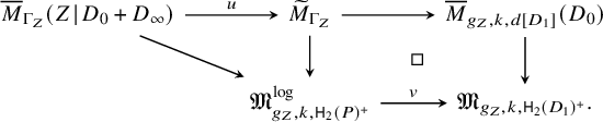
Then by [Reference van Garrel, Graber and Ruddat44, Theorem 4.1], we haveFootnote 5
 $$ \begin{align*} [\overline{M}_{\Gamma_Z}(Z \hspace{0.2ex}|\hspace{0.2ex} D_0 + D_\infty)]^{\mathrm{virt}} = u^!_{\mathfrak{E}_{\overline{M}_{\Gamma_Z}(Z \hspace{0.2ex}|\hspace{0.2ex} D_0 + D_\infty)/\widetilde{M}_{\Gamma_Z}}} v^! [\overline{M}_{g_Z,k, d[D_1]} (D_0)]^{\mathrm{virt}}\,. \end{align*} $$
Our claim that $[\overline {M}_{\Gamma _Z}(Z \hspace {0.2ex}|\hspace {0.2ex} D_0 + D_\infty )]^{\mathrm {virt}}=0$
directly follows from the fact that
$[\overline {M}_{\Gamma _Z}(Z \hspace {0.2ex}|\hspace {0.2ex} D_0 + D_\infty )]^{\mathrm {virt}}=0$
directly follows from the fact that
 $$ \begin{align*} [\overline{M}_{g_Z,k, d[D_1]} (D_0)]^{\mathrm{virt}} = 0 \end{align*} $$
since $D_0 \cong \operatorname *{\mathrm {Tot}} \mathcal {O}_{\mathbb {P}^1}(-2)$
carries a nowhere vanishing holomorphic two-form and
$D_0 \cong \operatorname *{\mathrm {Tot}} \mathcal {O}_{\mathbb {P}^1}(-2)$
carries a nowhere vanishing holomorphic two-form and $d>0$
.
$d>0$
.
4.4.2 Second vanishing: star shaped graphs
In this section, we apply the same arguments we used in Section 3.4.3 in order to constrain the shape of $\Gamma $
to star shaped graphs.
$\Gamma $
to star shaped graphs.
Notation 4.3. We introduce the following notation for labelling sets:
-
• Interior markings with a point condition
; -
• Contact markings with a point condition
; -
• Contact markings without an insertion
.
We may assume that all Z-vertices of $\Gamma $
are decorated with a curve class which is a multiple of a fibre class. This has the following consequence.
$\Gamma $
are decorated with a curve class which is a multiple of a fibre class. This has the following consequence.
Lemma 4.4. We have $[\overline {M}_{\Gamma _Z}(Z \hspace {0.2ex}|\hspace {0.2ex} D_0 + D_\infty )\lvert _{\mathcal {F}_0}]^{\mathrm {virt}} = 0$
unless every Z-vertex
$[\overline {M}_{\Gamma _Z}(Z \hspace {0.2ex}|\hspace {0.2ex} D_0 + D_\infty )\lvert _{\mathcal {F}_0}]^{\mathrm {virt}} = 0$
unless every Z-vertex
-
• either carries two legs, one labelled in
$I_{\mathrm {pt}}$
and one in ; -
• or carries a single leg with label in
$J_{\mathrm {pt}}$
.


Proof. It suffices to show that every Z-vertex is carrying at most one leg with label in $I_{\mathrm {pt}} \cup J_{\mathrm {pt}}$
. Indeed, in this case, the number of vertices in
$I_{\mathrm {pt}} \cup J_{\mathrm {pt}}$
. Indeed, in this case, the number of vertices in $\Gamma _Z$
is bounded from below by
$\Gamma _Z$
is bounded from below by $|I_{\mathrm {pt}}| + |J_{\mathrm {pt}}| = n$
. However, it is also bounded from above by the number of contact markings n. We deduce that there have to be exactly n vertices each carrying one of the legs labelled by
$|I_{\mathrm {pt}}| + |J_{\mathrm {pt}}| = n$
. However, it is also bounded from above by the number of contact markings n. We deduce that there have to be exactly n vertices each carrying one of the legs labelled by ![]() . Since we assumed that every vertex carries at most one leg with label in
. Since we assumed that every vertex carries at most one leg with label in $I_{\mathrm {pt}} \cup J_{\mathrm {pt}}$
, the m interior markings are necessarily distributed among the vertices carrying a leg labelled in
$I_{\mathrm {pt}} \cup J_{\mathrm {pt}}$
, the m interior markings are necessarily distributed among the vertices carrying a leg labelled in ![]() .
.
So suppose there is a Z-vertex with more than one leg with label in $I_{\mathrm {pt}} \cup J_{\mathrm {pt}}$
. Since the evaluation morphism of an interior marking has target Z, let us first define a substack with confined evaluations:
$I_{\mathrm {pt}} \cup J_{\mathrm {pt}}$
. Since the evaluation morphism of an interior marking has target Z, let us first define a substack with confined evaluations:
As every Z-vertex is decorated with a curve class which is a multiple of a fibre class and we assume there is a vertex with two legs labelled in $I_{\mathrm {pt}} \cup J_{\mathrm {pt}}$
, the resulting evaluation morphism
$I_{\mathrm {pt}} \cup J_{\mathrm {pt}}$
, the resulting evaluation morphism
 $$ \begin{align*} \overline{N}_{\Gamma_Z} \longrightarrow D_\infty^n \end{align*} $$
factors through $D_\infty ^{n-1} \rightarrow D_\infty ^n$
. We obtain the following commuting diagram with Cartesian squares:
$D_\infty ^{n-1} \rightarrow D_\infty ^n$
. We obtain the following commuting diagram with Cartesian squares:
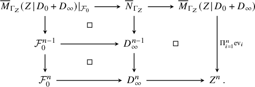
The vanishing of $[\overline {M}_{\Gamma _Z}(Z \hspace {0.2ex}|\hspace {0.2ex} D_0 + D_\infty )\lvert _{\mathcal {F}_0}]^{\mathrm {virt}}$
then immediately follows from an excess bundle calculation as the one we did in Lemma 3.8.
$[\overline {M}_{\Gamma _Z}(Z \hspace {0.2ex}|\hspace {0.2ex} D_0 + D_\infty )\lvert _{\mathcal {F}_0}]^{\mathrm {virt}}$
then immediately follows from an excess bundle calculation as the one we did in Lemma 3.8.
Moreover, by our assumption that all Z-vertices carry curve classes which are multiples of a fibre class, the evaluation morphism associated to edges
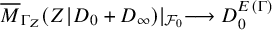 $$ \begin{align*} \overline{M}_{\Gamma_Z}(Z \hspace{0.2ex}|\hspace{0.2ex} D_0 + D_\infty)\lvert_{\mathcal{F}_0} \longrightarrow D_0^{E(\Gamma)} \end{align*} $$
factors through $F^{E(\Gamma )} \hookrightarrow D_0^{E(\Gamma )}$
, where we write F for the image of
$F^{E(\Gamma )} \hookrightarrow D_0^{E(\Gamma )}$
, where we write F for the image of $\mathcal {F}_0$
under
$\mathcal {F}_0$
under $Z\rightarrow D_0$
. We combine this observation with the fact that stable maps to Y factor through the zero section
$Z\rightarrow D_0$
. We combine this observation with the fact that stable maps to Y factor through the zero section $S\hookrightarrow Y$
in order to constrain the image of Z-vertices to the fibre of
$S\hookrightarrow Y$
in order to constrain the image of Z-vertices to the fibre of $Z\rightarrow D_0$
over the point
$Z\rightarrow D_0$
over the point $p = F \cap D_1$
. Indeed, as we just argued, the evaluation morphism
$p = F \cap D_1$
. Indeed, as we just argued, the evaluation morphism
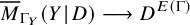 $$ \begin{align*} \overline{M}_{\Gamma_Y}(Y \hspace{0.2ex}|\hspace{0.2ex} D) \longrightarrow D^{E(\Gamma)} \end{align*} $$
factors through $D_1^{E(\Gamma )} \hookrightarrow D^{E(\Gamma )}$
. Writing
$D_1^{E(\Gamma )} \hookrightarrow D^{E(\Gamma )}$
. Writing $\overline {M}_{\Gamma _Y}(Y \hspace {0.2ex}|\hspace {0.2ex} D)\lvert _{F}$
for the fibre product
$\overline {M}_{\Gamma _Y}(Y \hspace {0.2ex}|\hspace {0.2ex} D)\lvert _{F}$
for the fibre product $\overline {M}_{\Gamma _Y}(Y \hspace {0.2ex}|\hspace {0.2ex} D)\times _{D^{E(\Gamma )}} F^{E(\Gamma )}$
, we find that
$\overline {M}_{\Gamma _Y}(Y \hspace {0.2ex}|\hspace {0.2ex} D)\times _{D^{E(\Gamma )}} F^{E(\Gamma )}$
, we find that
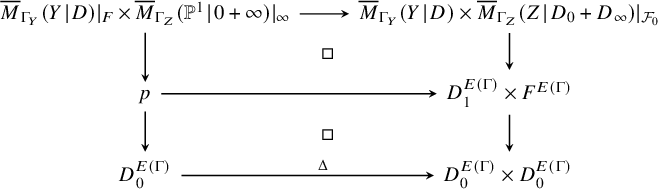
commutes and both squares are Cartesian. An excess intersection argument as in Lemma 3.9 gives the following.
Lemma 4.5. We have $[\overline {M}_\Gamma ]^{\mathrm {virt}}=0$
if there is a Z-vertex with more than one edge.
$[\overline {M}_\Gamma ]^{\mathrm {virt}}=0$
if there is a Z-vertex with more than one edge.
Since all squares in (4.9) are Cartesian, a comparison with (4.5) gives
 $$ \begin{align*} \overline{M}_{\Gamma} \cong \overline{M}_{\Gamma_Y}(Y \hspace{0.2ex}|\hspace{0.2ex} D)\lvert_{F}\,\times\, \overline{M}_{\Gamma_Z}(\mathbb{P}^1 \hspace{0.2ex}|\hspace{0.2ex} 0+\infty)\lvert_{\infty}\,. \end{align*} $$
The following lemma comparing the virtual fundamental classes of the above moduli stacks can be proven with the same arguments we used to show Lemma 3.10.
Lemma 4.6. If $\Gamma $
contains a Z-vertex v with
$\Gamma $
contains a Z-vertex v with $g_v>0$
, the cycle
$g_v>0$
, the cycle $[\overline {M}_\Gamma ]^{\mathrm {virt}}$
vanishes. Otherwise, it equates to
$[\overline {M}_\Gamma ]^{\mathrm {virt}}$
vanishes. Otherwise, it equates to
 $$\begin{align*} &[\overline{M}_{\Gamma_Y}(Y \hspace{0.2ex}|\hspace{0.2ex} D)\lvert_{F}]^{\mathrm{virt}} \times [\overline{M}_{\Gamma_Z}(\mathbb{P}^1 \hspace{0.2ex}|\hspace{0.2ex} 0+\infty)\lvert_{\infty}]^{\mathrm{virt}}. \end{align*}$$
Let us summarise the results of this section.
Proposition 4.7. The cycle $[\overline {M}_\Gamma ]^{\mathrm {virt}}$
vanishes unless the rigid tropical type
$[\overline {M}_\Gamma ]^{\mathrm {virt}}$
vanishes unless the rigid tropical type $\unicode{x3c4} $
associated to
$\unicode{x3c4} $
associated to $\Gamma $
is of the form
$\Gamma $
is of the form
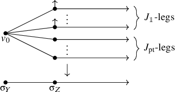
where $v_0$
is decorated with
$v_0$
is decorated with $g_{v_0}=g$
,
$g_{v_0}=g$
, $\unicode{x3b2} _{v_0}=\unicode{x3b2} $
and all other vertices are decorated with multiples of fibre classes. Moreover, in this case,
$\unicode{x3b2} _{v_0}=\unicode{x3b2} $
and all other vertices are decorated with multiples of fibre classes. Moreover, in this case,
 $$\begin{align*}&[\overline{M}_{\Gamma}]^{\mathrm{virt}} = [\overline{M}_{\Gamma_Y}(Y \hspace{0.2ex}|\hspace{0.2ex} D)\lvert_{F}]^{\mathrm{virt}} \times [\overline{M}_{\Gamma_Z}(\mathbb{P}^1 \hspace{0.2ex}|\hspace{0.2ex} 0+\infty)\lvert_{\infty}]^{\mathrm{virt}}.\end{align*}$$
4.5 Analysis of remaining terms
Now our discussion will deviate from the analysis in Section 3.4 because as opposed to Section 3.4.4, we will show that all remaining contributions characterised in Proposition 4.7 do contribute to the Gromov–Witten invariant and will exactly yield the right-hand side of equation (4.2).
Let $\Gamma $
be as in Proposition 4.7. We fix a labelling of the markings of
$\Gamma $
be as in Proposition 4.7. We fix a labelling of the markings of $\overline {M}_{\Gamma _Y}(Y \hspace {0.2ex}|\hspace {0.2ex} D)\lvert _{F}$
by fixing a bijection
$\overline {M}_{\Gamma _Y}(Y \hspace {0.2ex}|\hspace {0.2ex} D)\lvert _{F}$
by fixing a bijection $\{1,\ldots ,n\} \cong E(\Gamma )$
where we impose that the ith edge is adjacent to the Z-vertex carrying the
$\{1,\ldots ,n\} \cong E(\Gamma )$
where we impose that the ith edge is adjacent to the Z-vertex carrying the $(m+i)$
th leg. With this assignment, we can naturally identify
$(m+i)$
th leg. With this assignment, we can naturally identify $\Gamma _Y$
with the data
$\Gamma _Y$
with the data $(g,\mathbf {c},\unicode{x3b2} )$
.
$(g,\mathbf {c},\unicode{x3b2} )$
.
Our first goal is to simplify
Under $\unicode{x3b8} $
, all images of stable maps which lie in a fibre of
$\unicode{x3b8} $
, all images of stable maps which lie in a fibre of $P\rightarrow D_1$
get contracted to a point. Hence, the morphism factors into
$P\rightarrow D_1$
get contracted to a point. Hence, the morphism factors into

where $\unicode{x3c0} $
is the forgetful morphism which only remembers the stabilised domain curve and
$\unicode{x3c0} $
is the forgetful morphism which only remembers the stabilised domain curve and $\unicode{x3c6} $
is a morphism which forgets the logarithmic structure and attaches a contracted rational component at the last m markings.
$\unicode{x3c6} $
is a morphism which forgets the logarithmic structure and attaches a contracted rational component at the last m markings.
Consequently, a Z-vertex carrying a leg labelled with ![]() contributes with a factor
contributes with a factor
 $$ \begin{align*} \deg [\overline{M}_{0,((c_i,0),(0,c_i)),c_i}(\mathbb{P}^1 \hspace{0.2ex}|\hspace{0.2ex} 0+\infty)\lvert_{\infty}]^{\mathrm{virt}} = \deg [\overline{M}_{0,((c_i,0),(0,c_i)),c_i}(\mathbb{P}^1 \hspace{0.2ex}|\hspace{0.2ex} 0+\infty)]^{\mathrm{virt}} = \frac{1}{c_i}, \end{align*} $$
where the denominator is due to the degree $c_i$
automorphism group acting on the unique degree
$c_i$
automorphism group acting on the unique degree $c_i$
cover
$c_i$
cover $\mathbb {P}^1 \rightarrow \mathbb {P}^1$
fully ramified over
$\mathbb {P}^1 \rightarrow \mathbb {P}^1$
fully ramified over $0$
and infinity. Similarly, a Z-vertex with leg labelled by
$0$
and infinity. Similarly, a Z-vertex with leg labelled by $i+m \in J_{\mathrm {pt}}$
contributes
$i+m \in J_{\mathrm {pt}}$
contributes
 $$ \begin{align*} \deg [\overline{M}_{0,(0,(c_i,0),(0,c_i)),c_i}(\mathbb{P}^1 \hspace{0.2ex}|\hspace{0.2ex} 0+\infty)\lvert_{\infty}]^{\mathrm{virt}} = \deg \big( \mathrm{ev}_1^{*}(\mathrm{pt})\cap [\overline{M}_{0,(0,(c_i,0),(0,c_i)),c_i}(\mathbb{P}^1 \hspace{0.2ex}|\hspace{0.2ex} 0+\infty)]^{\mathrm{virt}} \big) = 1 \end{align*} $$
because the additional marking kills the automorphism group acting on the domain. We obtain
Note that a splitting type $\Gamma $
as in Proposition 4.7 is uniquely determined by the bijection
$\Gamma $
as in Proposition 4.7 is uniquely determined by the bijection ![]() it induces. This means there are exactly
it induces. This means there are exactly $m!$
such splitting types, each one contributing with (4.10) to the overall Gromov–Witten invariant. Thus, plugging the last equation into (4.8), we find
$m!$
such splitting types, each one contributing with (4.10) to the overall Gromov–Witten invariant. Thus, plugging the last equation into (4.8), we find
Pushing the identity forward to a point yields formula (4.2) which closes the proof of Proposition 4.1.
5 Applications
5.1 Topological Vertex
Open Gromov–Witten invariants can be computed efficiently using the topological vertex method [Reference Aganagic, Klemm, Mariño and Vafa4, Reference Li, Liu, Liu and Zhou30]. Hence, formula (2.7) equating logarithmic Gromov–Witten invariants – which are usually rather cumbersome to compute – against open ones presents a new venue for calculating the former.
5.1.1 The general recipe
We refer to [Reference Yu46, Section 2] or [Reference Bousseau, Brini and van Garrel11, Section 6] for a general summary of the topological vertex method which allows to determine the open Gromov–Witten invariants of a toric triple just from the information of its toric diagram. Let $(X,L,\mathsf {f})$
be the outcome of Construction 2.8 for some two-component Looijenga pair
$(X,L,\mathsf {f})$
be the outcome of Construction 2.8 for some two-component Looijenga pair $(Y\hspace {0.2ex}|\hspace {0.2ex} D_1 + D_2)$
. We will write
$(Y\hspace {0.2ex}|\hspace {0.2ex} D_1 + D_2)$
. We will write
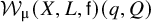 $$ \begin{align} \mathcal{W}_{\unicode{x3bc}}(X,L,\mathsf{f})(q,Q) \end{align} $$
for the generating series of disconnected open Gromov–Witten invariants of $(X,L,\mathsf {f})$
in representation basis where the winding around L is encoded in a partition
$(X,L,\mathsf {f})$
in representation basis where the winding around L is encoded in a partition $\unicode{x3bc} $
. In the special case of a single boundary wrapping the Lagrangian submanifold L, we can extract the connected invariant defined in (2.4) via [Reference Bousseau, Brini and van Garrel11, Equation (6.16)]Footnote
6
$\unicode{x3bc} $
. In the special case of a single boundary wrapping the Lagrangian submanifold L, we can extract the connected invariant defined in (2.4) via [Reference Bousseau, Brini and van Garrel11, Equation (6.16)]Footnote
6
 $$ \begin{align} \sum_{\unicode{x3b2}'} \sum_{g\geq 0} \mathsf{OGW}_{g,(c),\unicode{x3b2}'}(X,L,\mathsf{f}) ~ \hbar^{2g-1}\, Q^{\unicode{x3b2}'} = -\mathrm{i} \sum_{k=0}^c \frac{(-1)^k}{c} \frac{\mathcal{W}_{(c-k,1^k)}(X,L,\mathsf{f})}{\mathcal{W}_{\emptyset}(X,L,\mathsf{f})} \end{align} $$
under the change of variables $q=\mathrm {e}^{\mathrm {i} \hbar }$
where we fixed a square root
$q=\mathrm {e}^{\mathrm {i} \hbar }$
where we fixed a square root $\mathrm {i}$
of
$\mathrm {i}$
of $-1$
.
$-1$
.
The generating series $\mathcal {W}_{\unicode{x3bc} }(X,L,\mathsf {f})$
can be calculated algorithmically via the topological vertex method by performing a weighted sum over decorations of the toric diagram [Reference Aganagic, Klemm, Mariño and Vafa4, Reference Li, Liu, Liu and Zhou30]. As we discussed in Section 3.1, for our case at hand, the toric diagram of
$\mathcal {W}_{\unicode{x3bc} }(X,L,\mathsf {f})$
can be calculated algorithmically via the topological vertex method by performing a weighted sum over decorations of the toric diagram [Reference Aganagic, Klemm, Mariño and Vafa4, Reference Li, Liu, Liu and Zhou30]. As we discussed in Section 3.1, for our case at hand, the toric diagram of $(X,L,\mathsf {f})$
will have a shape as displayed in Figure 3. We label the compact one-dimensional torus orbit closures by
$(X,L,\mathsf {f})$
will have a shape as displayed in Figure 3. We label the compact one-dimensional torus orbit closures by $\ell _1,\ldots ,\ell _k$
starting from the stratum
$\ell _1,\ldots ,\ell _k$
starting from the stratum $\ell _0$
intersected by L and decorate each edge
$\ell _0$
intersected by L and decorate each edge $\ell _i$
with a partition
$\ell _i$
with a partition $\unicode{x3bc} _i$
as indicated in the figure. Then every edge
$\unicode{x3bc} _i$
as indicated in the figure. Then every edge $\ell _i$
,
$\ell _i$
, $i\in \{0,\ldots ,k\}$
, contributes with a factor
$i\in \{0,\ldots ,k\}$
, contributes with a factor
to (5.1), where ![]() . Each trivalent vertex corresponding to a torus fixed point
. Each trivalent vertex corresponding to a torus fixed point $\ell _i\cap \ell _{i+1}$
contributes
$\ell _i\cap \ell _{i+1}$
contributes
where, by convention, $\unicode{x3bc} _0=\unicode{x3bc} $
and
$\unicode{x3bc} _0=\unicode{x3bc} $
and $\unicode{x3bc} _{k+1}=\emptyset $
and
$\unicode{x3bc} _{k+1}=\emptyset $
and $s_{\unicode{x3b1} /\unicode{x3b2} } \big (q^{\unicode{x3c1} +\unicode{x3b3} }\big )$
denotes the skew Schur function
$s_{\unicode{x3b1} /\unicode{x3b2} } \big (q^{\unicode{x3c1} +\unicode{x3b3} }\big )$
denotes the skew Schur function $s_{\unicode{x3b1} /\unicode{x3b2} } \big (x_1,x_2,\ldots \big )$
evaluated at
$s_{\unicode{x3b1} /\unicode{x3b2} } \big (x_1,x_2,\ldots \big )$
evaluated at $x_j = q^{-j + \frac {1}{2} +\unicode{x3b3} _j}$
. As an application of [Reference Li, Liu, Liu and Zhou30, Proposition 7.4], we obtain
$x_j = q^{-j + \frac {1}{2} +\unicode{x3b3} _j}$
. As an application of [Reference Li, Liu, Liu and Zhou30, Proposition 7.4], we obtain
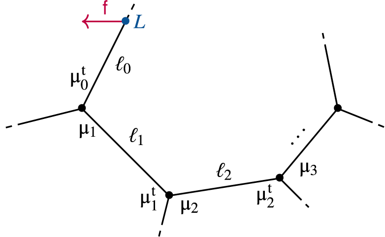
Figure 3 Toric diagram of $(X,L,\mathsf {f})$
decorated with partitions.
$(X,L,\mathsf {f})$
decorated with partitions.
Lemma 5.1. For $(X,L,\mathsf {f})$
the outcome of Construction 2.8, we have
$(X,L,\mathsf {f})$
the outcome of Construction 2.8, we have

In case the toric triple is a strip geometry, the above sum of partitions can be carried out explicitly to yield a closed form solution for $\mathcal {W}_{\unicode{x3bc} }(X,L,\mathsf {f})$
[Reference Iqbal and Kashani-Poor21]. Plugged into (5.2) and (2.7), this can be used to give a closed form solution for the logarithmic Gromov–Witten invariants of
$\mathcal {W}_{\unicode{x3bc} }(X,L,\mathsf {f})$
[Reference Iqbal and Kashani-Poor21]. Plugged into (5.2) and (2.7), this can be used to give a closed form solution for the logarithmic Gromov–Witten invariants of $(S\hspace {0.2ex}|\hspace {0.2ex} D_1+D_2)$
. We illustrate this method with an explicit example in the following section.
$(S\hspace {0.2ex}|\hspace {0.2ex} D_1+D_2)$
. We illustrate this method with an explicit example in the following section.
5.1.2 Extended example:
$\mathrm {dP}_3(0,2)$

Let us consider $(\mathrm {dP}_3 \hspace {0.2ex}|\hspace {0.2ex} D_1+D_2)$
where
$(\mathrm {dP}_3 \hspace {0.2ex}|\hspace {0.2ex} D_1+D_2)$
where $\mathrm {dP}_3$
is a del Pezzo surface which is the result of blowing up three points in
$\mathrm {dP}_3$
is a del Pezzo surface which is the result of blowing up three points in $\mathbb {P}^2$
. This Looijenga pair was denoted by
$\mathbb {P}^2$
. This Looijenga pair was denoted by $\mathrm {dP}_3(0,2)$
in [Reference Bousseau, Brini and van Garrel11]. If we write
$\mathrm {dP}_3(0,2)$
in [Reference Bousseau, Brini and van Garrel11]. If we write $E_1,E_2,E_3$
for exceptional divisors, we take
$E_1,E_2,E_3$
for exceptional divisors, we take $D_1\in |H-E_1|$
and
$D_1\in |H-E_1|$
and $D_2 \in |2H-E_2-E_3|$
smooth with transverse intersections. We use the following notation for a curve class in
$D_2 \in |2H-E_2-E_3|$
smooth with transverse intersections. We use the following notation for a curve class in $\mathrm {dP}_3$
:
$\mathrm {dP}_3$
:
 $$ \begin{align*} \unicode{x3b2} = d_0 (H-E_1-E_2-E_3) + d_1 E_1 +d_2 E_2 + d_3 E_3\,. \end{align*} $$
It was conjectured in [Reference Bousseau, Brini and van Garrel11] and later proven in [Reference Brini and Schuler12] that the maximum contact logarithmic Gromov–Witten invariants of this geometry have the following closed form solution.
Proposition 5.2 [Reference Brini and Schuler12, Proposition 1.4].
For all effective curve classes $\unicode{x3b2} $
in
$\unicode{x3b2} $
in $\mathrm {dP}_3$
with
$\mathrm {dP}_3$
with $D_i \cdot \unicode{x3b2}>0$
,
$D_i \cdot \unicode{x3b2}>0$
, $i\in \{1,2\}$
, and contact data
$i\in \{1,2\}$
, and contact data ![]() , we have
, we have
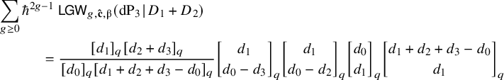 $$ \begin{align} \begin{aligned} &\sum_{g\geq 0} \hbar^{2g-1} ~ \mathsf{LGW}_{g,\mathbf{\hat{c}},\unicode{x3b2}}(\mathrm{dP}_3 \hspace{0.2ex}|\hspace{0.2ex} D_1+D_2) \\ & \hspace{3em}= \frac{[d_1]_q [d_2+d_3]_q}{[d_0]_q [d_1 + d_2 + d_3 - d_0]_q} \genfrac{[}{]}{0pt}{}{d_1}{d_0-d_3}_q \genfrac{[}{]}{0pt}{}{d_1}{d_0-d_2}_q \genfrac{[}{]}{0pt}{}{d_0}{d_1}_q \genfrac{[}{]}{0pt}{}{d_1+d_2+d_3-d_0}{d_1}_q \end{aligned} \end{align} $$
as formal Laurent series in $\hbar $
under the identification
$\hbar $
under the identification $q=\mathrm {e}^{\mathrm {i} \hbar }$
.
$q=\mathrm {e}^{\mathrm {i} \hbar }$
.
In this proposition, we use the notation
The statement was proven in [Reference Brini and Schuler12] by extracting the Gromov–Witten invariants from a quantum scattering diagram of a toric model of $(\mathrm {dP}_3 \hspace {0.2ex}|\hspace {0.2ex} D_1+D_2)$
. The outcome of this calculation is a convoluted sum of products of q-binomial coefficients which with a lot of effort can be simplified to yield the above formula. We will give a new proof of this identity using the topological vertex method.
$(\mathrm {dP}_3 \hspace {0.2ex}|\hspace {0.2ex} D_1+D_2)$
. The outcome of this calculation is a convoluted sum of products of q-binomial coefficients which with a lot of effort can be simplified to yield the above formula. We will give a new proof of this identity using the topological vertex method.
Proof of Proposition 5.2.
We start by applying Construction 2.8 to $(\mathrm {dP}_3 \hspace {0.2ex}|\hspace {0.2ex} D_1+D_2)$
. For this, let us write
$(\mathrm {dP}_3 \hspace {0.2ex}|\hspace {0.2ex} D_1+D_2)$
. For this, let us write $p_1,p_2,p_3$
for the three points in
$p_1,p_2,p_3$
for the three points in $\mathbb {P}^2$
whose blowup gives
$\mathbb {P}^2$
whose blowup gives $\mathrm {dP}_3$
. Then
$\mathrm {dP}_3$
. Then $D_1$
is the strict transform of a line through
$D_1$
is the strict transform of a line through $p_1$
and
$p_1$
and $D_2$
the strict transform of a conic through
$D_2$
the strict transform of a conic through $p_2$
and
$p_2$
and $p_3$
. We note that we can always choose the
$p_3$
. We note that we can always choose the $\mathbb {G}_{\mathsf {m}}^2$
-action on
$\mathbb {G}_{\mathsf {m}}^2$
-action on $\mathbb {P}^2$
in such a way that
$\mathbb {P}^2$
in such a way that $D_1$
is a toric hypersurface and
$D_1$
is a toric hypersurface and $p_1$
and
$p_1$
and $p_2$
are torus fixed points. Now with this choice of
$p_2$
are torus fixed points. Now with this choice of $\mathbb {G}_{\mathsf {m}}^2$
-action, the blowups at
$\mathbb {G}_{\mathsf {m}}^2$
-action, the blowups at $p_1$
and
$p_1$
and $p_2$
are toric as opposed to the one at
$p_2$
are toric as opposed to the one at $p_3$
since all points are assumed to be in general position. However, there is a deformation of
$p_3$
since all points are assumed to be in general position. However, there is a deformation of $\mathrm {dP}_3$
to the blowup of
$\mathrm {dP}_3$
to the blowup of $\mathbb {P}^2$
in
$\mathbb {P}^2$
in $p_1,p_2$
and a torus fixed point of
$p_1,p_2$
and a torus fixed point of $E_2$
leaving
$E_2$
leaving $D_1$
invariant. We denote this deformation by
$D_1$
invariant. We denote this deformation by $\mathrm {dP}^{\prime }_3$
which is indeed toric as required. We display its fan in Figure 4, where we labelled each ray with its curve class. Since
$\mathrm {dP}^{\prime }_3$
which is indeed toric as required. We display its fan in Figure 4, where we labelled each ray with its curve class. Since $\mathrm {dP}^{\prime }_3$
is toric with
$\mathrm {dP}^{\prime }_3$
is toric with $D_1$
a toric hypersurface, we can choose
$D_1$
a toric hypersurface, we can choose
 $$ \begin{align*} X = \operatorname*{\mathrm{Tot}} \mathcal{O}_{\mathrm{dP}^{\prime}_3} (-D_2) \lvert_{\mathrm{dP}^{\prime}_3 \setminus D_1}\,. \end{align*} $$
The toric diagram of $(X,L,\mathsf {f})$
is displayed in Figure 4 where we chose L to intersect the torus invariant curve in class
$(X,L,\mathsf {f})$
is displayed in Figure 4 where we chose L to intersect the torus invariant curve in class $H-E_2-E_3$
. We note that this particular toric triple has already been studied by Bousseau, Brini and van Garrel in [Reference Bousseau, Brini and van Garrel11, Section 6.3.1]. Hence, from here on we basically follow their calculation.
$H-E_2-E_3$
. We note that this particular toric triple has already been studied by Bousseau, Brini and van Garrel in [Reference Bousseau, Brini and van Garrel11, Section 6.3.1]. Hence, from here on we basically follow their calculation.
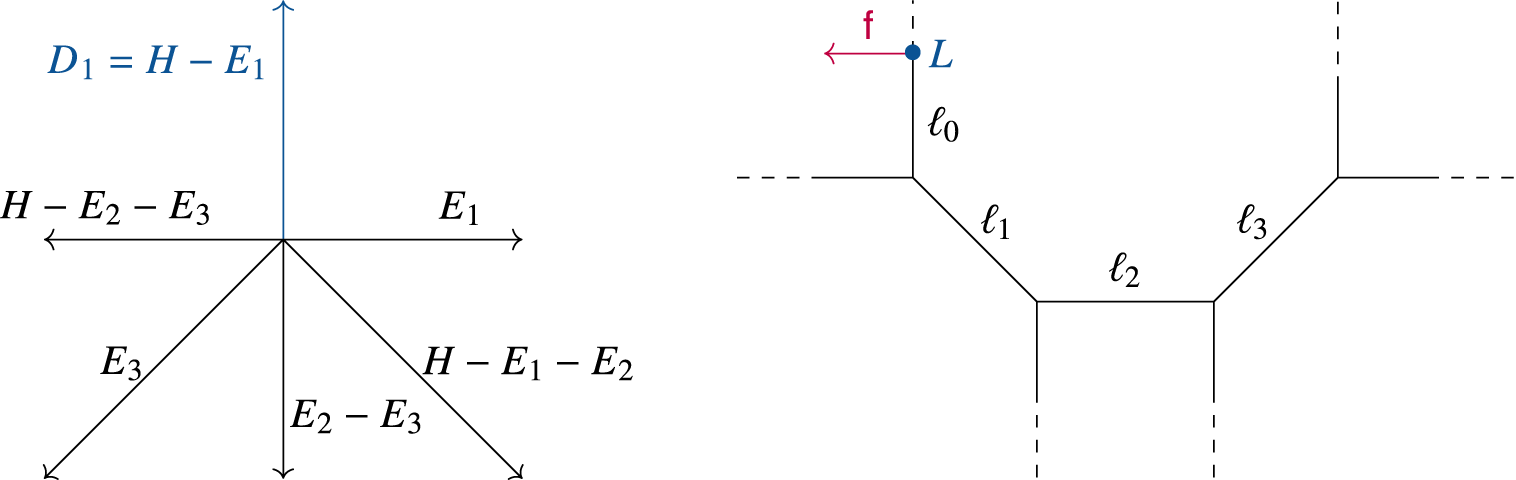
Figure 4 The fan of $\mathrm {dP}^{\prime }_3$
on the left and the toric diagram of
$\mathrm {dP}^{\prime }_3$
on the left and the toric diagram of $(X,L,\mathsf {f})$
on the right [Reference Bousseau, Brini and van Garrel11, Figure 6.5].
$(X,L,\mathsf {f})$
on the right [Reference Bousseau, Brini and van Garrel11, Figure 6.5].
Observe that each compact edge in the toric diagram corresponds to a ray in the fan. Hence, we can read off the degree of the normal bundles of $\ell _0,\ldots ,\ell _3$
from Figure 4 to be
$\ell _0,\ldots ,\ell _3$
from Figure 4 to be $-1$
,
$-1$
, $-1$
,
$-1$
, $-2$
and
$-2$
and $-1$
, respectively. Thus, by Lemma 5.1, we have
$-1$
, respectively. Thus, by Lemma 5.1, we have
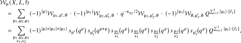
where to get the second line we used (5.3). This can now be plugged into (5.2) and simplified using the techniques developed in [Reference Iqbal and Kashani-Poor21]. These steps have already been carried out in [Reference Bousseau, Brini and van Garrel11, Equation (6.18–6.23)] and result in
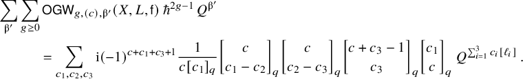 $$ \begin{align*} \begin{aligned} &\sum_{\unicode{x3b2}'} \sum_{g\geq 0} \mathsf{OGW}_{g,(c),\unicode{x3b2}'}(X,L,\mathsf{f}) ~ \hbar^{2g-1}\, Q^{\unicode{x3b2}'}\\ &\hspace{3em}= \sum_{c_1,c_2,c_3} \mathrm{i} (-1)^{c+c_1+c_3+1} \frac{1}{c [c_1]_q} \genfrac{[}{]}{0pt}{}{c}{c_1 -c_2}_q \genfrac{[}{]}{0pt}{}{c}{c_2 -c_3}_q \genfrac{[}{]}{0pt}{}{c+c_3-1}{c_3}_q \genfrac{[}{]}{0pt}{}{c_1}{c}_q ~ Q^{\sum_{i=1}^3 c_i [\ell_i]}\,. \end{aligned} \end{align*} $$
Extracting the coefficient of $Q^{\iota ^{*}(\unicode{x3b2} - d_1 [\ell _0])}$
from the above formula, we get
$Q^{\iota ^{*}(\unicode{x3b2} - d_1 [\ell _0])}$
from the above formula, we get
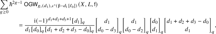 $$ \begin{align*} \begin{aligned} &\sum_{g\geq 0} \hbar^{2g-1} ~ \mathsf{OGW}_{g,(d_1),\iota^{*}(\unicode{x3b2} - d_1 [\ell_0])}(X,L,\mathsf{f})\\ &\hspace{3em} = \frac{\mathrm{i} (-1)^{d_1+d_2+d_3+1} [d_1]_q}{d_1 [d_0]_q [d_1 + d_2 + d_3 - d_0]_q} \genfrac{[}{]}{0pt}{}{d_1}{d_0-d_3}_q \genfrac{[}{]}{0pt}{}{d_1}{d_0-d_2}_q \genfrac{[}{]}{0pt}{}{d_0}{d_1}_q \genfrac{[}{]}{0pt}{}{d_1+d_2+d_3-d_0}{d_1}_q, \end{aligned} \end{align*} $$
which can be plugged into (2.7) to yield the formula stated in Proposition 5.2.
We stress that the above calculation is substantially easier than the one in [Reference Brini and Schuler12] using scattering diagrams. This hopefully illustrates the usefulness of our main result Theorem 2.9.
5.2 BPS integrality
It is a general feature rather than a coincidence that the all-genus generating series of logarithmic Gromov–Witten invariants lifts to a rational function in $\mathrm {e}^{\mathrm {i} \hbar }$
as we saw for instance in formula (5.4). This property is usually called BPS integrality.
$\mathrm {e}^{\mathrm {i} \hbar }$
as we saw for instance in formula (5.4). This property is usually called BPS integrality.
5.2.1 LMOV invariants
In the context of open Gromov–Witten invariants of toric Calabi–Yau threefolds, BPS integrality was first systematically studied by Labastida–Marino–Ooguri–Vafa [Reference Ooguri and Vafa41, Reference Labastida and Mariño26, Reference Labastida, Mariño and Vafa27, Reference Mariño and Vafa39]. Just recently, Yu gave a proof of this phenomenon by carefully analysing the combinatorics of the topological vertex [Reference Yu46].
To review Yu’s result, let $(X,L,\mathsf {f})$
be a toric triple. For a curve class
$(X,L,\mathsf {f})$
be a toric triple. For a curve class $\unicode{x3b2} ^{\prime }$
in X and a winding profile
$\unicode{x3b2} ^{\prime }$
in X and a winding profile $\mathbf {c}=(c_1,\ldots ,c_n)$
along L, we will write
$\mathbf {c}=(c_1,\ldots ,c_n)$
along L, we will write
 $$ \begin{align*} k \hspace{0.2ex}|\hspace{0.2ex} (\mathbf{c},\unicode{x3b2}^{\prime}) \end{align*} $$
for $k\in \mathbb {N}$
if k divides
$k\in \mathbb {N}$
if k divides $c_i$
for all
$c_i$
for all $i\in \{1,\ldots ,n\}$
and there is a curve class
$i\in \{1,\ldots ,n\}$
and there is a curve class $\unicode{x3b2} ^{\prime \prime }$
satisfying
$\unicode{x3b2} ^{\prime \prime }$
satisfying $k\unicode{x3b2} ^{\prime \prime }=\unicode{x3b2} ^{\prime }$
.
$k\unicode{x3b2} ^{\prime \prime }=\unicode{x3b2} ^{\prime }$
.
Now for every tuple $(\mathbf {c},\unicode{x3b2} ^{\prime })$
, we define
$(\mathbf {c},\unicode{x3b2} ^{\prime })$
, we define
by demanding that these formal power series satisfy

Writing $\unicode{x3bc} $
for the Möbius function, one can check that
$\unicode{x3bc} $
for the Möbius function, one can check that
 $$ \begin{align*} \mathsf{LMOV}_{\mathbf{c},\unicode{x3b2}^{\prime}}(\hbar) = \left(2 \sin \tfrac{\hbar}{2}\right)^2 \prod_{i=1}^n \frac{c_i}{2 \sin \tfrac{\hbar c_i}{2}} ~ \sum_{k | (\mathbf{c},\unicode{x3b2}^{\prime})} \frac{\unicode{x3bc}(k)}{k} \sum_{g\geq 0} (k\hbar)^{2g-2+n} ~ \mathsf{OGW}_{g,\mathbf{c}/k,\unicode{x3b2}^{\prime}/k}(X,L,\mathsf{f}) \end{align*} $$
is indeed a solution to the above defining equation.
Theorem 5.3 ((LMOV integrality). [Reference Yu46, Theorem 1.1]). $\mathsf {LMOV}_{\mathbf {c},\unicode{x3b2} ^{\prime }}$
lifts to a Laurent polynomial in
$\mathsf {LMOV}_{\mathbf {c},\unicode{x3b2} ^{\prime }}$
lifts to a Laurent polynomial in $q=\mathrm {e}^{\mathrm {i} \hbar }$
with integer coefficients.
$q=\mathrm {e}^{\mathrm {i} \hbar }$
with integer coefficients.
5.2.2 BPS integrality of logarithmic invariants
Now let $(S\hspace {0.2ex}|\hspace {0.2ex} D_1+D_2)$
be a logarithmic Calabi–Yau surface with boundary the union of two transversally intersecting smooth curves
$(S\hspace {0.2ex}|\hspace {0.2ex} D_1+D_2)$
be a logarithmic Calabi–Yau surface with boundary the union of two transversally intersecting smooth curves $D_1,D_2$
. To a tuple
$D_1,D_2$
. To a tuple $(\mathbf {\hat {c}},\unicode{x3b2} )$
, where
$(\mathbf {\hat {c}},\unicode{x3b2} )$
, where $\unicode{x3b2} $
is an effective curve class in S satisfying
$\unicode{x3b2} $
is an effective curve class in S satisfying $D_1 \cdot \unicode{x3b2} \geq 0$
and
$D_1 \cdot \unicode{x3b2} \geq 0$
and $D_2 \cdot \unicode{x3b2}> 0$
and
$D_2 \cdot \unicode{x3b2}> 0$
and $\mathbf {\hat {c}}$
is a contact condition of the form
$\mathbf {\hat {c}}$
is a contact condition of the form

for some $c_1,\ldots ,c_n>0$
and
$c_1,\ldots ,c_n>0$
and $m\leq n$
, we associate a formal power series
$m\leq n$
, we associate a formal power series
solving the recursive system
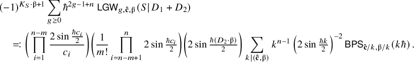
Again, one can check that
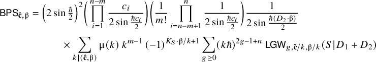 $$ \begin{align*} \begin{aligned} \mathsf{BPS}_{\mathbf{\hat{c}},\unicode{x3b2}} &= \left(2 \sin \tfrac{\hbar}{2}\right)^2 \bigg(\prod_{i=1}^{n-m} \frac{c_i}{2 \sin \tfrac{\hbar c_i}{2}} \bigg) \bigg(\frac{1}{m!}\prod_{i=n-m+1}^{n} \frac{1}{2 \sin \tfrac{\hbar c_i}{2}} \bigg) \frac{1}{2 \sin \tfrac{\hbar (D_2 \cdot \unicode{x3b2})}{2}} \\[0.3em] & \hspace{3em}\times\sum_{k | (\mathbf{\hat{c}},\unicode{x3b2})} \unicode{x3bc}(k) \, k^{m-1} \, (-1)^{K_S \cdot \unicode{x3b2} /k +1} \sum_{g\geq 0} (k\hbar)^{2g-1+n} ~ \mathsf{LGW}_{g,\mathbf{\hat{c}}/k,\unicode{x3b2}/k}(S \hspace{0.2ex}|\hspace{0.2ex} D_1+D_2) \end{aligned} \end{align*} $$
is indeed a solution to this defining equation. Motivated by the last section, we expect the following.
Conjecture 5.4. $\mathsf {BPS}_{\hat {c},\unicode{x3b2} }$
lifts to a Laurent polynomial in
$\mathsf {BPS}_{\hat {c},\unicode{x3b2} }$
lifts to a Laurent polynomial in $q=\mathrm {e}^{\mathrm {i} \hbar }$
with integer coefficients.
$q=\mathrm {e}^{\mathrm {i} \hbar }$
with integer coefficients.
Evidence for the conjecture comes from the following immediate corollary of Yu’s LMOV integrality (Theorem 5.3) and our logarithmic-open correspondence (Theorem 2.9).
Theorem 5.5. Conjecture 5.4 holds if $(S \hspace {0.2ex}|\hspace {0.2ex} D_1 + D_2)$
satisfies Assumption ★. Especially, if
$(S \hspace {0.2ex}|\hspace {0.2ex} D_1 + D_2)$
satisfies Assumption ★. Especially, if $(X,L,\mathsf {f})$
is the toric triple from Construction 2.8, we have
$(X,L,\mathsf {f})$
is the toric triple from Construction 2.8, we have
 $$\begin{align*}& \mathsf{BPS}_{\mathbf{\hat{c}},\unicode{x3b2}} = \mathsf{LMOV}_{\mathbf{c},\unicode{x3b2}^{\prime}}.\end{align*}$$
Note that the pattern in which the sine factors enter the right-hand side of equation (5.5) naturally suggests a generalisation to the case where we permit more than one point of contact with $D_2$
. It remains to be seen whether BPS integrality persists in this case as well.
$D_2$
. It remains to be seen whether BPS integrality persists in this case as well.
Acknowledgements
First and foremost, I would like to thank my supervisor Andrea Brini for suggesting this project, and for innumerous discussions and his continuous support. Special thanks are also due to Cristina Manolache for clarifying discussions concerning key steps in the proof of our main result. I also benefited from discussions with Alberto Cobos Rábano, Michel van Garrel, Samuel Johnston, Navid Nabijou, Dhruv Ranganathan, Ajith Urundolil Kumaran and Song Yu which I am highly grateful for.
Parts of this work have been carried out during research visits at the University of Cambridge. I thank the university and St John’s College for hospitality and financial support.
During the publication process, the author was employed at ETH Zürich, Department of Mathematics supported by the SNF grant SNF-200020-21936.
Competing interest
The authors have no competing interests to declare.


 Open access