


1 Introduction
1.1 Background and motivation
Let
 $(X,\omega _0)$
be a compact Kähler manifold, and let
$(X,\omega _0)$
be a compact Kähler manifold, and let
 $\omega ^{\bullet }(t),t\in [0,T)$
be a family of Kähler metrics on X which solve the Kähler-Ricci flow
$\omega ^{\bullet }(t),t\in [0,T)$
be a family of Kähler metrics on X which solve the Kähler-Ricci flow
 $$ \begin{align} \partial_t\omega^{\bullet} (t)=-\textrm{Ric}(\omega^{\bullet} (t))-\omega^{\bullet}(t), \quad \omega^{\bullet} (0)=\omega_0 \end{align} $$
for some
 $0<T\leqslant +\infty $
. In this paper, we are interested in the case when
$0<T\leqslant +\infty $
. In this paper, we are interested in the case when
 $\omega ^{\bullet }(t)$
is an immortal solution (i.e., when
$\omega ^{\bullet }(t)$
is an immortal solution (i.e., when
 $T=+\infty $
). Thanks to a result of Tian-Zhang [Reference Tian and Zhang37] (see also [Reference Tsuji45]), we know that the solution
$T=+\infty $
). Thanks to a result of Tian-Zhang [Reference Tian and Zhang37] (see also [Reference Tsuji45]), we know that the solution
 $\omega ^{\bullet }(t)$
is immortal if and only if the canonical bundle
$\omega ^{\bullet }(t)$
is immortal if and only if the canonical bundle
 $K_X$
is nef, which means that
$K_X$
is nef, which means that
 $c_1(K_X)$
lies in the closure of the cone of Kähler classes in
$c_1(K_X)$
lies in the closure of the cone of Kähler classes in
 $H^{1,1}(X,\mathbb {R})$
. This condition does not depend on
$H^{1,1}(X,\mathbb {R})$
. This condition does not depend on
 $\omega _0$
, and manifolds with
$\omega _0$
, and manifolds with
 $K_X$
nef are also known as smooth minimal models.
$K_X$
nef are also known as smooth minimal models.
The Abundance Conjecture in birational geometry, and its natural extension to Kähler manifolds, predicts that if the canonical bundle of a compact Kähler manifold is nef, then it must be semiample, which means that
 $K_X^p$
is base-point-free for some
$K_X^p$
is base-point-free for some
 $p\geqslant 1$
. This conjecture is known when
$p\geqslant 1$
. This conjecture is known when
 $\dim X\leqslant 3$
by [Reference Campana, Höring and Peternell1, Reference Das and Ou6, Reference Das and Ou7].
$\dim X\leqslant 3$
by [Reference Campana, Höring and Peternell1, Reference Das and Ou6, Reference Das and Ou7].
Throughout the rest of the paper, we will assume that
 $K_X$
is semiample. It is then known (see, for example, [Reference Lazarsfeld25, Theorem 2.1.27]) that global sections of
$K_X$
is semiample. It is then known (see, for example, [Reference Lazarsfeld25, Theorem 2.1.27]) that global sections of
 $K_X^p$
for
$K_X^p$
for
 $p\geqslant 1$
sufficiently divisible define a surjective holomorphic map
$p\geqslant 1$
sufficiently divisible define a surjective holomorphic map
 $f:X\to B\subset \mathbb {CP}^N$
(the Iitaka fibration of X) with connected fibers onto a normal projective variety B (known as the canonical model of X), of dimension m equal to the Kodaira dimension of X (in particular, we have
$f:X\to B\subset \mathbb {CP}^N$
(the Iitaka fibration of X) with connected fibers onto a normal projective variety B (known as the canonical model of X), of dimension m equal to the Kodaira dimension of X (in particular, we have
 $0\leqslant m\leqslant \dim X$
). The smooth fibers of f are then Calabi-Yau manifolds, of dimension
$0\leqslant m\leqslant \dim X$
). The smooth fibers of f are then Calabi-Yau manifolds, of dimension
 $n:=\dim X-m$
, which are pairwise diffeomorphic but in general are not pairwise biholomorphic.
$n:=\dim X-m$
, which are pairwise diffeomorphic but in general are not pairwise biholomorphic.
In the two extreme cases when
 $m=0$
or
$m=0$
or
 $m=\dim X$
, the behavior of the flow is completely understood thanks to the work of many people (see, for example, the recent survey [Reference Tosatti42] and references therein), so we will furthermore assume from now on that
$m=\dim X$
, the behavior of the flow is completely understood thanks to the work of many people (see, for example, the recent survey [Reference Tosatti42] and references therein), so we will furthermore assume from now on that
 $0<m<\dim X$
, which is known as ‘intermediate Kodaira dimension’. Thus, we have
$0<m<\dim X$
, which is known as ‘intermediate Kodaira dimension’. Thus, we have
 $\dim X=m+n$
, and both the fibers and the base of f are positive-dimensional.
$\dim X=m+n$
, and both the fibers and the base of f are positive-dimensional.
The simplest examples of this setup arise when
 $m=n=1$
, where X is a minimal properly elliptic surface, B is a compact Riemann surface, and
$m=n=1$
, where X is a minimal properly elliptic surface, B is a compact Riemann surface, and
 $f:X\to B$
is an elliptic fibration. In this case, the behavior of the Kähler-Ricci flow (1.1) was first studied by Song-Tian [Reference Song and Tian31], who shortly afterwards also considered the case of general
$f:X\to B$
is an elliptic fibration. In this case, the behavior of the Kähler-Ricci flow (1.1) was first studied by Song-Tian [Reference Song and Tian31], who shortly afterwards also considered the case of general
 $m,n$
in [Reference Song and Tian32]. A major difficulty in this setting is that the total volume of
$m,n$
in [Reference Song and Tian32]. A major difficulty in this setting is that the total volume of
 $(X,\omega ^{\bullet }(t))$
is easily seen to converge to zero as
$(X,\omega ^{\bullet }(t))$
is easily seen to converge to zero as
 $t\to +\infty $
, and this ‘collapsing’ behavior makes it extremely hard to analyze the flow. As we will now explain, in [Reference Song and Tian31, Reference Song and Tian32], it was shown that the metrics
$t\to +\infty $
, and this ‘collapsing’ behavior makes it extremely hard to analyze the flow. As we will now explain, in [Reference Song and Tian31, Reference Song and Tian32], it was shown that the metrics
 $\omega ^{\bullet }(t)$
collapse in the weak topology to the pullback of a canonical metric on B, and our main goal is to obtain higher order regularity and a uniform Ricci curvature bound for
$\omega ^{\bullet }(t)$
collapse in the weak topology to the pullback of a canonical metric on B, and our main goal is to obtain higher order regularity and a uniform Ricci curvature bound for
 $\omega ^{\bullet }(t)$
(away from the singular fibers of f) and thus prove two conjectures of Song-Tian.
$\omega ^{\bullet }(t)$
(away from the singular fibers of f) and thus prove two conjectures of Song-Tian.
When X is projective, the condition that
 $K_X$
be nef means that X is a smooth minimal model. The connection between the Minimal Model Program in birational geometry and the behavior of the Kähler-Ricci flow was first discovered independently by Cascini-La Nave [Reference Cascini and La Nave3] and Song-Tian [Reference Song and Tian31], and remains an area of current research. These works outlined a conjectural picture for the behavior of the Kähler-Ricci flow on any projective (or more generally compact Kähler) manifold. When
$K_X$
be nef means that X is a smooth minimal model. The connection between the Minimal Model Program in birational geometry and the behavior of the Kähler-Ricci flow was first discovered independently by Cascini-La Nave [Reference Cascini and La Nave3] and Song-Tian [Reference Song and Tian31], and remains an area of current research. These works outlined a conjectural picture for the behavior of the Kähler-Ricci flow on any projective (or more generally compact Kähler) manifold. When
 $K_X$
is not nef, singularities must develop in finite time, and the flow should implement the corresponding birational contractions or collapse the fibers of a Mori fiber space. The case when
$K_X$
is not nef, singularities must develop in finite time, and the flow should implement the corresponding birational contractions or collapse the fibers of a Mori fiber space. The case when
 $K_X$
is nef (so the manifold is a smooth minimal model) is the topic of our paper.
$K_X$
is nef (so the manifold is a smooth minimal model) is the topic of our paper.
1.2 Setup
We now describe our setup in more detail. As mentioned above, we have a compact Kähler manifold
 $(X^{m+n},\omega _0)$
with semiample canonical bundle and intermediate Kodaira dimension m (so
$(X^{m+n},\omega _0)$
with semiample canonical bundle and intermediate Kodaira dimension m (so
 $m,n>0$
), and
$m,n>0$
), and
 $\omega ^{\bullet }(t)$
denotes the immortal solution of the Kähler-Ricci flow (1.1). Let
$\omega ^{\bullet }(t)$
denotes the immortal solution of the Kähler-Ricci flow (1.1). Let
 $f:X\to B$
be the Iitaka fibration of X, and let
$f:X\to B$
be the Iitaka fibration of X, and let
 $S\subset X$
be the preimage of the union of the set of singular values of f and the singular set of B. Thus, by construction,
$S\subset X$
be the preimage of the union of the set of singular values of f and the singular set of B. Thus, by construction,
 $f:X\backslash S\to B\backslash f(S)$
is a proper holomorphic submersion with n-dimensional connected Calabi-Yau fibers
$f:X\backslash S\to B\backslash f(S)$
is a proper holomorphic submersion with n-dimensional connected Calabi-Yau fibers
 $X_{z}=f^{-1}(z), z\in B\backslash f(S)$
. By Ehresmann’s Lemma (and the connectedness of
$X_{z}=f^{-1}(z), z\in B\backslash f(S)$
. By Ehresmann’s Lemma (and the connectedness of
 $B\backslash f(S)$
), the fibers
$B\backslash f(S)$
), the fibers
 $X_z$
are pairwise diffeomorphic, but, in general, their complex structure varies with z, and this variation can be encoded in a smooth semipositive Weil-Petersson form
$X_z$
are pairwise diffeomorphic, but, in general, their complex structure varies with z, and this variation can be encoded in a smooth semipositive Weil-Petersson form
 $\omega _{\mathrm {WP}}\geqslant 0$
on
$\omega _{\mathrm {WP}}\geqslant 0$
on
 $B\backslash f(S)$
, defined in [Reference Song and Tian31] (see also [Reference Tosatti39, §5.6]).
$B\backslash f(S)$
, defined in [Reference Song and Tian31] (see also [Reference Tosatti39, §5.6]).
By [Reference Song and Tian32], there exists a smooth Kähler metric
 $\omega _{\mathrm {can}}$
on
$\omega _{\mathrm {can}}$
on
 $B\backslash f(S)$
satisfying the twisted Kähler-Einstein equation
$B\backslash f(S)$
satisfying the twisted Kähler-Einstein equation
 $$ \begin{align} \textrm{Ric}(\omega_{\mathrm{can}})=-\omega_{\mathrm{can}}+\omega_{\mathrm{WP}}. \end{align} $$
The pullback of
 $\omega _{\mathrm {can}}$
to
$\omega _{\mathrm {can}}$
to
 $X\backslash S$
will also be denoted by the same symbol, for convenience. The metric
$X\backslash S$
will also be denoted by the same symbol, for convenience. The metric
 $\omega _{\mathrm {can}}$
extends to a closed positive current on B, and in [Reference Song and Tian31, Reference Song and Tian32] it is shown that as
$\omega _{\mathrm {can}}$
extends to a closed positive current on B, and in [Reference Song and Tian31, Reference Song and Tian32] it is shown that as
 $t\to +\infty $
, we have
$t\to +\infty $
, we have
 $$ \begin{align} \omega^{\bullet}(t)\to \omega_{\mathrm{can}}, \end{align} $$
weakly as currents on X as well as in the
 $C^{0}_{\mathrm {loc}}(X\backslash S)$
topology of Kähler potentials. Motivated by this, in [Reference Song and Tian31, p.612], [Reference Song and Tian32, p.306], [Reference Tian35, Conjecture 4.5.7], [Reference Tian36, p.258], Song-Tian posed the following:
$C^{0}_{\mathrm {loc}}(X\backslash S)$
topology of Kähler potentials. Motivated by this, in [Reference Song and Tian31, p.612], [Reference Song and Tian32, p.306], [Reference Tian35, Conjecture 4.5.7], [Reference Tian36, p.258], Song-Tian posed the following:
Conjecture 1.1. Let
 $(X,\omega _0)$
be a compact Kähler manifold with
$(X,\omega _0)$
be a compact Kähler manifold with
 $K_X$
semiample and intermediate Kodaira dimension
$K_X$
semiample and intermediate Kodaira dimension
 $0<m<\dim X$
, and let
$0<m<\dim X$
, and let
 $\omega ^{\bullet }(t)$
solve (1.1). Then the convergence (1.3) happens in the locally smooth topology as tensors on
$\omega ^{\bullet }(t)$
solve (1.1). Then the convergence (1.3) happens in the locally smooth topology as tensors on
 $X\backslash S$
.
$X\backslash S$
.
Explicitly, Conjecture 1.1 asks to show that given any
 $K\Subset X\backslash S$
and
$K\Subset X\backslash S$
and
 $k\in \mathbb {N}$
, we have
$k\in \mathbb {N}$
, we have
 $$ \begin{align} \|\omega^{\bullet}(t)-\omega_{\mathrm{can}}\|_{C^k(K,g_0)}\to 0. \end{align} $$
There have been a number of partial results towards Conjecture 1.1, often using techniques that were first developed for a family of elliptic PDEs that describe the collapsing of families of Ricci-flat Kähler metrics on a Calabi-Yau manifold with a fibration structure, and which share some of the features of (1.1) (see, for example, the survey [Reference Tosatti40]). Indeed, Fong-Zhang [Reference Fong and Zhang12] adapted work of the third-named author [Reference Tosatti38] to prove that (1.3) holds in the
 $C^{1,\alpha }_{\mathrm { loc}}(X\backslash S)$
topology of Kähler potentials (
$C^{1,\alpha }_{\mathrm { loc}}(X\backslash S)$
topology of Kähler potentials (
 $\alpha <1$
), and the works [Reference Fong and Zhang12, Reference Hein and Tosatti19, Reference Tosatti and Zhang44] proved Conjecture 1.1 when the smooth fibers of f are tori or finite quotients of tori (see also [Reference Gill13] and [Reference Tosatti39, §5.14]), using and improving a method of Gross-Tosatti-Zhang [Reference Gross, Tosatti and Zhang14]. Later, Tosatti-Weinkove-Yang proved that (1.3) holds in
$\alpha <1$
), and the works [Reference Fong and Zhang12, Reference Hein and Tosatti19, Reference Tosatti and Zhang44] proved Conjecture 1.1 when the smooth fibers of f are tori or finite quotients of tori (see also [Reference Gill13] and [Reference Tosatti39, §5.14]), using and improving a method of Gross-Tosatti-Zhang [Reference Gross, Tosatti and Zhang14]. Later, Tosatti-Weinkove-Yang proved that (1.3) holds in
 $C^0_{\mathrm {loc}}(X\backslash S)$
, and this was improved to
$C^0_{\mathrm {loc}}(X\backslash S)$
, and this was improved to
 $C^{\alpha }_{\mathrm {loc}}(X\backslash S),\alpha <1$
by Chu-Lee [Reference Chu and Lee4] adapting the techniques of Hein-Tosatti [Reference Hein and Tosatti20], which also allowed Fong-Lee [Reference Fong and Lee11] to prove Conjecture 1.1 when all smooth fibers are pairwise biholomorphic.
$C^{\alpha }_{\mathrm {loc}}(X\backslash S),\alpha <1$
by Chu-Lee [Reference Chu and Lee4] adapting the techniques of Hein-Tosatti [Reference Hein and Tosatti20], which also allowed Fong-Lee [Reference Fong and Lee11] to prove Conjecture 1.1 when all smooth fibers are pairwise biholomorphic.
In a later work [Reference Song and Tian33], Song-Tian proved that the scalar curvature of
 $\omega ^{\bullet }(t)$
remains uniformly bounded on X, independent of
$\omega ^{\bullet }(t)$
remains uniformly bounded on X, independent of
 $t\geqslant 0$
. They then conjectured a similar statement for the Ricci curvature, away from the singular fibers of f (see [Reference Tian36, Conjecture 4.7]):
$t\geqslant 0$
. They then conjectured a similar statement for the Ricci curvature, away from the singular fibers of f (see [Reference Tian36, Conjecture 4.7]):
Conjecture 1.2. Let
 $(X,\omega _0)$
be a compact Kähler manifold with
$(X,\omega _0)$
be a compact Kähler manifold with
 $K_X$
semiample and intermediate Kodaira dimension
$K_X$
semiample and intermediate Kodaira dimension
 $0<m<\dim X$
, and let
$0<m<\dim X$
, and let
 $\omega ^{\bullet }(t)$
solve (1.1). Then the Ricci curvature of
$\omega ^{\bullet }(t)$
solve (1.1). Then the Ricci curvature of
 $\omega ^{\bullet }(t)$
remains uniformly bounded on compact subsets of
$\omega ^{\bullet }(t)$
remains uniformly bounded on compact subsets of
 $X\backslash S$
, independent of t.
$X\backslash S$
, independent of t.
This is only known when the smooth fibers of f are tori, or finite quotients of tori [Reference Fong and Lee11] (hence, in particular, it holds on minimal properly elliptic surfaces), or when the smooth fibers are pairwise biholomorphic [Reference Chu and Lee4]. It is known that, in general, the conjectural Ricci bound cannot be improved to a full Riemann curvature bound (on compact subsets of
 $X\backslash S$
): by [Reference Tosatti and Zhang44], this holds if and only if the smooth fibers are tori or finite quotients.
$X\backslash S$
): by [Reference Tosatti and Zhang44], this holds if and only if the smooth fibers are tori or finite quotients.
It is well known that the Kähler-Ricci flow (1.1) reduces to a scalar PDE, of parabolic complex Monge-Ampère type, for a family of evolving Kähler potentials. Following [Reference Song and Tian32], we construct a closed real
 $(1,1)$
-form
$(1,1)$
-form
 $\omega _F$
on
$\omega _F$
on
 $X\backslash S$
, which is of the form
$X\backslash S$
, which is of the form
 $\omega _F=\omega _0+{i\partial \bar \partial }\rho $
, such that for every
$\omega _F=\omega _0+{i\partial \bar \partial }\rho $
, such that for every
 $z\in B\backslash f(S)$
, we have that
$z\in B\backslash f(S)$
, we have that
 $\omega _F|_{X_z}$
is the unique Ricci-flat Kähler metric on
$\omega _F|_{X_z}$
is the unique Ricci-flat Kähler metric on
 $X_z$
cohomologous to
$X_z$
cohomologous to
 $\omega _0|_{X_z}$
. While
$\omega _0|_{X_z}$
. While
 $\omega _F$
is not semipositive definite in general (see [Reference Cao, Guenancia and Păun2] for a counterexample), given any compact set
$\omega _F$
is not semipositive definite in general (see [Reference Cao, Guenancia and Păun2] for a counterexample), given any compact set
 $K\Subset X\backslash S$
, we can find
$K\Subset X\backslash S$
, we can find
 $t_0$
such that for all
$t_0$
such that for all
 $t\geqslant t_0$
,
$t\geqslant t_0$
,
 $$ \begin{align} \omega^\natural(t):=(1-e^{-t})\omega_{\mathrm{can}}+e^{-t}\omega_F \end{align} $$
is a Kähler metric on K, with fibers of size
 $\approx e^{-t/2}$
and base of size
$\approx e^{-t/2}$
and base of size
 $\approx 1$
. On
$\approx 1$
. On
 $X\backslash S$
, we can then write
$X\backslash S$
, we can then write
 $\omega ^{\bullet }(t)=\omega ^\natural (t)+{i\partial \bar \partial }\varphi (t)$
, where the potentials
$\omega ^{\bullet }(t)=\omega ^\natural (t)+{i\partial \bar \partial }\varphi (t)$
, where the potentials
 $\varphi (t)$
satisfy
$\varphi (t)$
satisfy
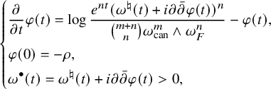 $$ \begin{align} \left\{ \begin{aligned} &\frac{\partial}{\partial t}\varphi (t)=\log\frac{e^{nt}(\omega^\natural(t)+{i\partial\bar\partial}\varphi (t))^n}{\binom{m+n}{n}\omega_{\mathrm{can}}^m\wedge\omega_F^n}-\varphi (t),\\ &\varphi (0)=-\rho,\\ &\omega^{\bullet}(t)=\omega^\natural(t)+{i\partial\bar\partial}\varphi (t)>0, \end{aligned} \right. \end{align} $$
for
 $t\geqslant 0$
(see, for example, [Reference Tosatti39, §5.7] and [Reference Tosatti, Weinkove and Yang43, §3.1]. Then, since we know the weak convergence in (1.3), Conjecture 1.1 is equivalent to the a priori estimates
$t\geqslant 0$
(see, for example, [Reference Tosatti39, §5.7] and [Reference Tosatti, Weinkove and Yang43, §3.1]. Then, since we know the weak convergence in (1.3), Conjecture 1.1 is equivalent to the a priori estimates
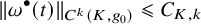 $$ \begin{align} \|\omega^{\bullet}(t)\|_{C^k(K,g_0)}\leqslant C_{K,k} \end{align} $$
for all
 $k\in \mathbb {N}$
and all
$k\in \mathbb {N}$
and all
 $t\geqslant 0$
. Furthermore, since
$t\geqslant 0$
. Furthermore, since
 $\varphi (t)$
is uniformly bounded in
$\varphi (t)$
is uniformly bounded in
 $L^\infty (X)$
by [Reference Song and Tian32] (which uses [Reference Demailly and Pali8, Reference Eyssidieux, Guedj and Zeriahi9] – see also [Reference Guo, Phong and Tong17] for a new proof), these estimates are also equivalent to
$L^\infty (X)$
by [Reference Song and Tian32] (which uses [Reference Demailly and Pali8, Reference Eyssidieux, Guedj and Zeriahi9] – see also [Reference Guo, Phong and Tong17] for a new proof), these estimates are also equivalent to
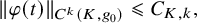 $$ \begin{align} \|\varphi (t)\|_{C^k(K,g_0)}\leqslant C_{K,k}, \end{align} $$
for all
 $k\in \mathbb {N}$
and all
$k\in \mathbb {N}$
and all
 $t\geqslant 0$
.
$t\geqslant 0$
.
1.3 Main result
The main result of this paper gives a complete solution of Conjectures 1.1 and 1.2:
In fact, in both conjectures, we prove much more precise statements. The higher order estimates for
 $\omega ^{\bullet }(t)$
are derived as consequences of a very detailed asymptotic expansion for
$\omega ^{\bullet }(t)$
are derived as consequences of a very detailed asymptotic expansion for
 $\omega ^{\bullet }(t)$
, which is in the same spirit as the expansion recently obtained in [Reference Hein and Tosatti21] by Hein-Tosatti for collapsing Ricci-flat metrics on Calabi-Yau manifolds. As for the Ricci curvature bound, we show that on
$\omega ^{\bullet }(t)$
, which is in the same spirit as the expansion recently obtained in [Reference Hein and Tosatti21] by Hein-Tosatti for collapsing Ricci-flat metrics on Calabi-Yau manifolds. As for the Ricci curvature bound, we show that on
 $X\backslash S$
we have
$X\backslash S$
we have
 $$ \begin{align} \textrm{Ric}(\omega^{\bullet}(t))=-\omega_{\mathrm{can}}+\mathrm{Err}, \end{align} $$
where on any fixed compact subset of
 $X\backslash S$
we have
$X\backslash S$
we have
 $|\mathrm {Err}|_{g^{\bullet }(t)}\to 0$
, as
$|\mathrm {Err}|_{g^{\bullet }(t)}\to 0$
, as
 $t\to +\infty $
. Thus, in a strong sense, the Ricci curvature of the evolving metrics
$t\to +\infty $
. Thus, in a strong sense, the Ricci curvature of the evolving metrics
 $\omega ^{\bullet }(t)$
is asymptotic to
$\omega ^{\bullet }(t)$
is asymptotic to
 $-\omega _{\mathrm {can}}$
. Furthermore, our bound on the Ricci curvature (and on all of the pieces of the asymptotic expansion of the metric) is an a priori bound: it only depends on the uniform constants in Lemma 4.1, which are due to [Reference Fong and Zhang12, Reference Song and Tian33, Reference Tosatti, Weinkove and Yang43].
$-\omega _{\mathrm {can}}$
. Furthermore, our bound on the Ricci curvature (and on all of the pieces of the asymptotic expansion of the metric) is an a priori bound: it only depends on the uniform constants in Lemma 4.1, which are due to [Reference Fong and Zhang12, Reference Song and Tian33, Reference Tosatti, Weinkove and Yang43].
The starting point of our analysis, which was proved in [Reference Fong and Zhang12] by adapting [Reference Tosatti38] in the elliptic setting, is the following estimate: given
 $K\Subset X\backslash S$
, there is
$K\Subset X\backslash S$
, there is
 $C>0$
such that on K we have
$C>0$
such that on K we have
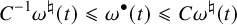 $$ \begin{align} C^{-1}\omega^\natural(t)\leqslant \omega^{\bullet}(t)\leqslant C\omega^\natural(t) \end{align} $$
for all
 $t\geqslant t_0$
. In other words,
$t\geqslant t_0$
. In other words,
 $\omega ^{\bullet }(t)$
is shrinking in the fiber directions and remains of bounded size in the base directions. Since the linearized operator of (1.6) is the time-dependent heat operator of
$\omega ^{\bullet }(t)$
is shrinking in the fiber directions and remains of bounded size in the base directions. Since the linearized operator of (1.6) is the time-dependent heat operator of
 $\omega ^{\bullet }(t)$
, we see from (1.10) that the ellipticity is degenerating in the fiber directions as
$\omega ^{\bullet }(t)$
, we see from (1.10) that the ellipticity is degenerating in the fiber directions as
 $t\to +\infty $
, and so there is no clear way to approach the a priori estimates (1.8). Indeed, the local analog of such estimates are false; see the discussion in [Reference Hein and Tosatti20] in the elliptic case.
$t\to +\infty $
, and so there is no clear way to approach the a priori estimates (1.8). Indeed, the local analog of such estimates are false; see the discussion in [Reference Hein and Tosatti20] in the elliptic case.
However, it turns out that we can work locally on the base (but using crucially that the fibers are compact without boundary), and since f is differentiably a locally trivial fiber bundle over
 $B\backslash f(S)$
, we may without loss assume that our base B is now simply the Euclidean unit ball in
$B\backslash f(S)$
, we may without loss assume that our base B is now simply the Euclidean unit ball in
 $\mathbb {C}^m$
, and
$\mathbb {C}^m$
, and
 $f:B\times Y\to B$
is just the projection onto the first factor, where Y is a closed manifold and
$f:B\times Y\to B$
is just the projection onto the first factor, where Y is a closed manifold and
 $B\times Y$
is equipped with a complex structure J (not necessarily a product) such that f is
$B\times Y$
is equipped with a complex structure J (not necessarily a product) such that f is
 $(J,J_{\mathbb {C}^m})$
holomorphic. The fibers
$(J,J_{\mathbb {C}^m})$
holomorphic. The fibers
 $\{z\}\times Y, z\in B$
are then compact n-dimensional Calabi-Yau manifolds diffeomorphic to Y. Under this trivialization, the Ricci-flat Kähler metric
$\{z\}\times Y, z\in B$
are then compact n-dimensional Calabi-Yau manifolds diffeomorphic to Y. Under this trivialization, the Ricci-flat Kähler metric
 $\omega _F|_{X_z}$
defines a Riemannian metric
$\omega _F|_{X_z}$
defines a Riemannian metric
 $g_{Y,z}$
on
$g_{Y,z}$
on
 $\{z\}\times Y$
, which we extend trivially to
$\{z\}\times Y$
, which we extend trivially to
 $B\times Y$
, and we use these to define a family of shrinking Riemannian product metrics
$B\times Y$
, and we use these to define a family of shrinking Riemannian product metrics
 $$ \begin{align} g_z(t)=g_{\mathbb{C}^m}+e^{-t}g_{Y,z}, \end{align} $$
on
 $B\times Y$
, which are uniformly equivalent to
$B\times Y$
, which are uniformly equivalent to
 $\omega ^\natural (t)$
and hence to
$\omega ^\natural (t)$
and hence to
 $\omega ^{\bullet }(t)$
. We will also denote by
$\omega ^{\bullet }(t)$
. We will also denote by
 $g(t):=g_0(t)$
the shrinking product metrics with z equal to the origin in B.
$g(t):=g_0(t)$
the shrinking product metrics with z equal to the origin in B.
1.4 Overview of the proof
As in [Reference Hein and Tosatti20, Reference Hein and Tosatti21], the first attempt to overcome the issue of degenerating ellipticity is to try to prove much more – namely, try to prove uniform bounds for
 $\varphi (t)$
or
$\varphi (t)$
or
 $\omega ^{\bullet }(t)$
in the shrinking norms
$\omega ^{\bullet }(t)$
in the shrinking norms
 $C^k(K,g(t))$
, since
$C^k(K,g(t))$
, since
 $g^{\bullet }(t)$
is uniformly equivalent to
$g^{\bullet }(t)$
is uniformly equivalent to
 $g(t)$
. This, however, cannot be proved in general since we know from [Reference Tosatti, Weinkove and Yang43] that
$g(t)$
. This, however, cannot be proved in general since we know from [Reference Tosatti, Weinkove and Yang43] that
 $e^t\omega ^{\bullet }(t)|_{X_z}$
converge smoothly to
$e^t\omega ^{\bullet }(t)|_{X_z}$
converge smoothly to
 $\omega _F|_{X_z}$
, and since
$\omega _F|_{X_z}$
, and since
 $g_{Y,z}$
and
$g_{Y,z}$
and
 $g_{Y,z'}$
are not in general parallel with respect to each other, the shrinking
$g_{Y,z'}$
are not in general parallel with respect to each other, the shrinking
 $C^k$
norms of
$C^k$
norms of
 $g_{z}(t)$
and
$g_{z}(t)$
and
 $g_{z'}(t)$
are not uniformly equivalent as
$g_{z'}(t)$
are not uniformly equivalent as
 $t\to +\infty $
. To address this issue, the first and third-named authors defined in [Reference Hein and Tosatti21] a connection
$t\to +\infty $
. To address this issue, the first and third-named authors defined in [Reference Hein and Tosatti21] a connection
 ${\mathbb {D}}$
on
${\mathbb {D}}$
on
 $B\times Y$
which on each fiber
$B\times Y$
which on each fiber
 $\{z\}\times Y$
acts like the Levi-Civita connection of
$\{z\}\times Y$
acts like the Levi-Civita connection of
 $g_z(t)$
, and using its parallel transport operator, they defined new shrinking
$g_z(t)$
, and using its parallel transport operator, they defined new shrinking
 $C^{k,\alpha }$
norms,
$C^{k,\alpha }$
norms,
 $0<\alpha <1$
. We will consider the natural parabolic extension of these norms to space-time derivatives in Section 2 below. Since parabolic Hölder seminorms behave differently according to the parity of k, we will only work with
$0<\alpha <1$
. We will consider the natural parabolic extension of these norms to space-time derivatives in Section 2 below. Since parabolic Hölder seminorms behave differently according to the parity of k, we will only work with
 $k=2j$
even (cf. Remark 2.5).
$k=2j$
even (cf. Remark 2.5).
The hope would then be to show that
 $\omega ^{\bullet }(t)-\omega ^\natural (t)={i\partial \bar \partial }\varphi (t)$
is uniformly bounded in these shrinking
$\omega ^{\bullet }(t)-\omega ^\natural (t)={i\partial \bar \partial }\varphi (t)$
is uniformly bounded in these shrinking
 $C^{2j+\alpha ,j+{\alpha }/2}$
norms. This turns out to be true when
$C^{2j+\alpha ,j+{\alpha }/2}$
norms. This turns out to be true when
 $j=0$
, but false starting from
$j=0$
, but false starting from
 $j=1$
. This phenomenon, which was discovered in [Reference Hein and Tosatti21] in the elliptic setting, manifests itself only when the complex structure J is not a product and the fibers are not tori or quotients. In a nutshell, the variation of complex structures, and the non-flatness of
$j=1$
. This phenomenon, which was discovered in [Reference Hein and Tosatti21] in the elliptic setting, manifests itself only when the complex structure J is not a product and the fibers are not tori or quotients. In a nutshell, the variation of complex structures, and the non-flatness of
 $g_{z}(t)$
, destroy these desired shrinking norm bounds. However, with much work, we are able to construct a collection of ‘obstruction functions’ on
$g_{z}(t)$
, destroy these desired shrinking norm bounds. However, with much work, we are able to construct a collection of ‘obstruction functions’ on
 $B\times Y$
(up to shrinking B) and decompose the solution
$B\times Y$
(up to shrinking B) and decompose the solution
 ${i\partial \bar \partial }\varphi (t)$
into a sum of finitely many terms
${i\partial \bar \partial }\varphi (t)$
into a sum of finitely many terms
 $\gamma _1(t),\dots ,\gamma _j(t)$
(constructed roughly speaking using the fiberwise
$\gamma _1(t),\dots ,\gamma _j(t)$
(constructed roughly speaking using the fiberwise
 $L^2$
projections of
$L^2$
projections of
 $\Delta ^{g^\natural (t)}\varphi (t)$
onto the space of obstructions), and a remainder
$\Delta ^{g^\natural (t)}\varphi (t)$
onto the space of obstructions), and a remainder
 $\eta _j(t)$
. We then show via a contradiction and blowup argument that the remainder
$\eta _j(t)$
. We then show via a contradiction and blowup argument that the remainder
 $\eta _j(t)$
is bounded in the shrinking
$\eta _j(t)$
is bounded in the shrinking
 $C^{2j+\alpha ,j+{\alpha }/2}$
norm, while the terms
$C^{2j+\alpha ,j+{\alpha }/2}$
norm, while the terms
 $\gamma _1(t),\dots ,\gamma _j(t)$
are not, but they satisfy strong enough estimates which guarantee that they are bounded in the
$\gamma _1(t),\dots ,\gamma _j(t)$
are not, but they satisfy strong enough estimates which guarantee that they are bounded in the
 $C^{2j+\alpha ,j+{\alpha }/2}$
norm of a fixed metric
$C^{2j+\alpha ,j+{\alpha }/2}$
norm of a fixed metric
 $\omega _X$
on X. As mentioned earlier, the higher order estimates on all these pieces depend only on the constant in the
$\omega _X$
on X. As mentioned earlier, the higher order estimates on all these pieces depend only on the constant in the
 $C^0$
estimate (1.10), and on the other constants that appear in Lemma 4.1 (including the uniform bound on the scalar curvature of
$C^0$
estimate (1.10), and on the other constants that appear in Lemma 4.1 (including the uniform bound on the scalar curvature of
 $\omega ^{\bullet }(t)$
from [Reference Song and Tian33]), and thus ultimately, they depend only on the geometry of X and on the initial metric
$\omega ^{\bullet }(t)$
from [Reference Song and Tian33]), and thus ultimately, they depend only on the geometry of X and on the initial metric
 $\omega _0$
.
$\omega _0$
.
This procedure is iterated by replacing j with
 $j+1$
, and new obstruction functions are constructed by measuring the failure of the remainder
$j+1$
, and new obstruction functions are constructed by measuring the failure of the remainder
 $\eta _j(t)$
to be bounded in the shrinking
$\eta _j(t)$
to be bounded in the shrinking
 $C^{2(j+1)+\alpha ,j+1+{\alpha }/2}$
norm. This way, we can split
$C^{2(j+1)+\alpha ,j+1+{\alpha }/2}$
norm. This way, we can split
 $\eta _j(t)=\gamma _{j+1}(t)+\eta _{j+1}(t)$
and obtain the next order in the expansion. As in [Reference Hein and Tosatti21], there is an extra technical difficulty, which arises from the fact that the terms
$\eta _j(t)=\gamma _{j+1}(t)+\eta _{j+1}(t)$
and obtain the next order in the expansion. As in [Reference Hein and Tosatti21], there is an extra technical difficulty, which arises from the fact that the terms
 $\gamma _j(t)$
are constructed by plugging in
$\gamma _j(t)$
are constructed by plugging in
 $\eta _{j-1}(t)$
and the obstruction functions into an approximate elliptic Green operator, which has an extra parameter
$\eta _{j-1}(t)$
and the obstruction functions into an approximate elliptic Green operator, which has an extra parameter
 $k\in \mathbb {N}$
that measures the quality of the approximation. Thus, all the terms in the expansion also end up depending on k, which is large and chosen a priori, and the procedure works for
$k\in \mathbb {N}$
that measures the quality of the approximation. Thus, all the terms in the expansion also end up depending on k, which is large and chosen a priori, and the procedure works for
 $j\leqslant k$
.
$j\leqslant k$
.
The resulting asymptotic expansion of
 $\omega ^{\bullet }(t)$
is described in detail in Theorem 4.2 below, which is the main technical result of the paper. It is the parabolic analog of [Reference Hein and Tosatti21, Theorem 4.1], and its proof follows the same overall method via blowup and contradiction, but there are some new key difficulties. First, as mentioned earlier, the (shrinking) parabolic Hölder norms that we use are better behaved when the order of derivatives is even, which compels us to use
$\omega ^{\bullet }(t)$
is described in detail in Theorem 4.2 below, which is the main technical result of the paper. It is the parabolic analog of [Reference Hein and Tosatti21, Theorem 4.1], and its proof follows the same overall method via blowup and contradiction, but there are some new key difficulties. First, as mentioned earlier, the (shrinking) parabolic Hölder norms that we use are better behaved when the order of derivatives is even, which compels us to use
 $C^{2j+\alpha ,j+{\alpha }/2}$
norms instead of
$C^{2j+\alpha ,j+{\alpha }/2}$
norms instead of
 $C^{j+\alpha ,(j+{\alpha })/2}$
(see, for example, Lemma 2.4 and Remark 2.5). More importantly, since the approximate Green operator that we use in this paper is the same as in [Reference Hein and Tosatti21], it provides an approximate parametrix for the Laplacian of
$C^{j+\alpha ,(j+{\alpha })/2}$
(see, for example, Lemma 2.4 and Remark 2.5). More importantly, since the approximate Green operator that we use in this paper is the same as in [Reference Hein and Tosatti21], it provides an approximate parametrix for the Laplacian of
 $\omega ^\natural (t)$
(in a rough sense) but not for the heat operator (it seems far from clear that a similar strategy could be implemented with an approximate heat kernel construction). Because of this, to obtain a contradiction at the end of the blowup argument (which is divided into 3 cases, with the last case itself divided into 3 subcases A, B and C), we now have to deal with new terms that come from taking time derivatives of the solution, which are not taken care of by construction, unlike [Reference Hein and Tosatti21]. To make matters worse, in the blowup argument, the evolving Kähler potential has
$\omega ^\natural (t)$
(in a rough sense) but not for the heat operator (it seems far from clear that a similar strategy could be implemented with an approximate heat kernel construction). Because of this, to obtain a contradiction at the end of the blowup argument (which is divided into 3 cases, with the last case itself divided into 3 subcases A, B and C), we now have to deal with new terms that come from taking time derivatives of the solution, which are not taken care of by construction, unlike [Reference Hein and Tosatti21]. To make matters worse, in the blowup argument, the evolving Kähler potential has
 $L^\infty $
norm that is blowing up, so it cannot be passed to a limit to obtain a contradiction. Dealing with these issues requires substantial work.
$L^\infty $
norm that is blowing up, so it cannot be passed to a limit to obtain a contradiction. Dealing with these issues requires substantial work.
Another new difficulty, compared to [Reference Hein and Tosatti21], is that the case
 $j=0$
(i.e., where we prove
$j=0$
(i.e., where we prove
 $C^{{\alpha },{\alpha }/2}$
estimates) does not behave in the same way as the cases
$C^{{\alpha },{\alpha }/2}$
estimates) does not behave in the same way as the cases
 $j\geqslant 1$
because the parabolic complex Monge-Ampère equation also involves
$j\geqslant 1$
because the parabolic complex Monge-Ampère equation also involves
 $\varphi (t)$
without derivatives landing on it, unlike the elliptic complex Monge-Ampère equation where only
$\varphi (t)$
without derivatives landing on it, unlike the elliptic complex Monge-Ampère equation where only
 ${i\partial \bar \partial }\varphi $
enters. To deal with this issue, we employ a different blowup quantity for
${i\partial \bar \partial }\varphi $
enters. To deal with this issue, we employ a different blowup quantity for
 $j=0$
, which is closer in spirit to our earlier works [Reference Hein and Tosatti20, Reference Fong and Lee11]. As a result, different ideas will be required to close the blowup argument, according to whether
$j=0$
, which is closer in spirit to our earlier works [Reference Hein and Tosatti20, Reference Fong and Lee11]. As a result, different ideas will be required to close the blowup argument, according to whether
 $j=0$
or
$j=0$
or
 $j\geqslant 1$
. Furthermore, when
$j\geqslant 1$
. Furthermore, when
 $j\geqslant 1$
, we are forced to add one new term to the main blowup quantity (when compared to [Reference Hein and Tosatti21]), to gain better control on the fiber average of the Kähler potential and its time derivative, and we later have to show that this new term can be dealt with in the blowup argument. Next, in subcase A, dealing with these terms forces us to refine the Selection Theorem 3.1 where the obstruction functions are chosen, and when
$j\geqslant 1$
, we are forced to add one new term to the main blowup quantity (when compared to [Reference Hein and Tosatti21]), to gain better control on the fiber average of the Kähler potential and its time derivative, and we later have to show that this new term can be dealt with in the blowup argument. Next, in subcase A, dealing with these terms forces us to refine the Selection Theorem 3.1 where the obstruction functions are chosen, and when
 $j=0$
, we need a whole new argument. In subcase B, we employ an energy argument inspired by [Reference Fong and Lee11, Claim 3.2], and in subcase C a different energy argument has to be applied fiber by fiber.
$j=0$
, we need a whole new argument. In subcase B, we employ an energy argument inspired by [Reference Fong and Lee11, Claim 3.2], and in subcase C a different energy argument has to be applied fiber by fiber.
Once the asymptotic expansion is established, the smooth convergence of Conjecture 1.1 follows easily. However, proving the Ricci curvature bound for
 $\omega ^{\bullet }(t)$
in Conjecture 1.2 requires substantial work by plugging in the expansion with
$\omega ^{\bullet }(t)$
in Conjecture 1.2 requires substantial work by plugging in the expansion with
 $j=1$
into the formula for the Ricci curvature (as two derivatives of the logarithm of the volume form) and using our explicit a priori estimates for the terms of the expansion to deduce boundedness of Ricci. Here again, we encounter a new difficulty compared to [Reference Hein and Tosatti21], which arises from the fact that one of the estimates in Theorem 4.2 is weaker than the corresponding one in the elliptic setting, because of the fact that we can only work with even order norms. During the course of the proof of the Ricci bound, we also prove a fact of independent interest in Proposition 5.1, by showing that
$j=1$
into the formula for the Ricci curvature (as two derivatives of the logarithm of the volume form) and using our explicit a priori estimates for the terms of the expansion to deduce boundedness of Ricci. Here again, we encounter a new difficulty compared to [Reference Hein and Tosatti21], which arises from the fact that one of the estimates in Theorem 4.2 is weaker than the corresponding one in the elliptic setting, because of the fact that we can only work with even order norms. During the course of the proof of the Ricci bound, we also prove a fact of independent interest in Proposition 5.1, by showing that
 $\varphi +\dot {\varphi }$
minus its fiberwise average decays to zero (away from the singular fibers) faster than
$\varphi +\dot {\varphi }$
minus its fiberwise average decays to zero (away from the singular fibers) faster than
 $e^{-t}$
(see (5.33)). This improves on earlier work of Fong-Zhang [Reference Fong and Zhang12, p.110] (see also [Reference Tosatti39, Lemma 5.13]) and Tosatti-Weinkove-Yang [Reference Tosatti, Weinkove and Yang43, Lemma 3.1 (iv)].
$e^{-t}$
(see (5.33)). This improves on earlier work of Fong-Zhang [Reference Fong and Zhang12, p.110] (see also [Reference Tosatti39, Lemma 5.13]) and Tosatti-Weinkove-Yang [Reference Tosatti, Weinkove and Yang43, Lemma 3.1 (iv)].
Remark 1.4. We conjecture that the Ricci curvature of
 $\omega ^{\bullet }(t)$
remains uniformly bounded also near the singular fibers of f. One could imagine settling this for some minimal elliptic surfaces by developing a parabolic version of the Gross-Wilson gluing result in [Reference Gross and Wilson15] (thanks to J. Lott for this suggestion), and for some Lefschetz fibered
$\omega ^{\bullet }(t)$
remains uniformly bounded also near the singular fibers of f. One could imagine settling this for some minimal elliptic surfaces by developing a parabolic version of the Gross-Wilson gluing result in [Reference Gross and Wilson15] (thanks to J. Lott for this suggestion), and for some Lefschetz fibered
 $3$
-folds by developing a parabolic version of Li’s gluing result in [Reference Li27].
$3$
-folds by developing a parabolic version of Li’s gluing result in [Reference Li27].
Remark 1.5. It is natural to ask whether we really need to assume that our compact Kähler manifold X with
 $K_X$
nef satisfies the Abundance Conjecture (thanks to S. Karigiannis and J. Cheng for raising this point). The reader can verify that the results in [Reference Fong and Zhang12, Reference Song and Tian32, Reference Song and Tian33, Reference Tosatti, Weinkove and Yang43] on which we rely, as well as our main theorems, are also valid under the a priori weaker assumption that
$K_X$
nef satisfies the Abundance Conjecture (thanks to S. Karigiannis and J. Cheng for raising this point). The reader can verify that the results in [Reference Fong and Zhang12, Reference Song and Tian32, Reference Song and Tian33, Reference Tosatti, Weinkove and Yang43] on which we rely, as well as our main theorems, are also valid under the a priori weaker assumption that
 $c_1(K_X)$
is a semiample
$c_1(K_X)$
is a semiample
 $(1,1)$
-class [Reference Tosatti41, Def.3.4]: there is a surjective holomorphic map
$(1,1)$
-class [Reference Tosatti41, Def.3.4]: there is a surjective holomorphic map
 $f:X\to B$
with connected fibers onto a normal compact Kähler analytic space B such that
$f:X\to B$
with connected fibers onto a normal compact Kähler analytic space B such that
 $c_1(K_X)=f^{*}[\omega ]$
for some Kähler class
$c_1(K_X)=f^{*}[\omega ]$
for some Kähler class
 $[\omega ]$
on B. However, a very recent result of Das-Hacon [Reference Das and Hacon5, Theorem 4.4], which was prompted by our questions to C. Hacon as well as the related [Reference Tosatti41, Question 3.5], shows that under this hypothesis
$[\omega ]$
on B. However, a very recent result of Das-Hacon [Reference Das and Hacon5, Theorem 4.4], which was prompted by our questions to C. Hacon as well as the related [Reference Tosatti41, Question 3.5], shows that under this hypothesis
 $K_X$
is already semiample, and it is elementary to deduce from this that f is the Iitaka fibration of
$K_X$
is already semiample, and it is elementary to deduce from this that f is the Iitaka fibration of
 $K_X$
. We thank also M. Păun for discussions about this point.
$K_X$
. We thank also M. Păun for discussions about this point.
1.5 Organization of the paper
In Section 2 we introduce our parabolic shrinking norms and seminorms and prove an interpolation inequality, the crucial Proposition 2.6 and a Schauder estimate. Section 3 contains the proof of the Selection Theorem 3.1 where the obstruction functions are selected. Section 4 is the main part of the paper and is where the asymptotic expansion is proved in Theorem 4.2. Lastly, in Section 5, we give the proof of our main Theorem 1.3.
2 Parabolic Hölder norms and interpolation
The setup where we are working in was described in the Introduction.
2.1
 ${\mathbb {D}}$
-derivatives
${\mathbb {D}}$
-derivatives

Recall that our main goal is to establish higher order estimates for the metrics
 $\omega ^{\bullet }(t)$
on
$\omega ^{\bullet }(t)$
on
 $B\times Y$
which evolve by the normalized Kähler-Ricci flow (1.1). We know from Lemma 4.1 (i) below that
$B\times Y$
which evolve by the normalized Kähler-Ricci flow (1.1). We know from Lemma 4.1 (i) below that
 $\omega ^{\bullet }(t)$
is uniformly equivalent to
$\omega ^{\bullet }(t)$
is uniformly equivalent to
 $\omega ^\natural (t)=(1-e^{-t})\omega _{\mathrm {can}}+e^{-t}\omega _F$
, which is shrinking in the fiber directions as
$\omega ^\natural (t)=(1-e^{-t})\omega _{\mathrm {can}}+e^{-t}\omega _F$
, which is shrinking in the fiber directions as
 $t\to +\infty $
. As mentioned above in the overview of proof, the fiberwise Ricci-flat metrics
$t\to +\infty $
. As mentioned above in the overview of proof, the fiberwise Ricci-flat metrics
 $g_{Y,z}$
are in general quite different from each other as
$g_{Y,z}$
are in general quite different from each other as
 $z\in B$
varies, and this forces us to define a new connection
$z\in B$
varies, and this forces us to define a new connection
 ${\mathbb {D}}$
which along each fiber
${\mathbb {D}}$
which along each fiber
 $\{z\}\times Y$
acts like the Levi-Civita connection of
$\{z\}\times Y$
acts like the Levi-Civita connection of
 $g_z(t)=g_{\mathbb {C}^m}+e^{-t}g_{Y,z}$
. This is what was achieved by the first and third-named authors in [Reference Hein and Tosatti21, §2.1], and we now recall their construction.
$g_z(t)=g_{\mathbb {C}^m}+e^{-t}g_{Y,z}$
. This is what was achieved by the first and third-named authors in [Reference Hein and Tosatti21, §2.1], and we now recall their construction.
Definition 2.1. For
 $z\in B\subset \mathbb {C}^m$
, we let
$z\in B\subset \mathbb {C}^m$
, we let
 $\nabla ^z$
be the Levi-Civita connection of the product metric
$\nabla ^z$
be the Levi-Civita connection of the product metric
 $g_{z}(t)=g_{\mathbb {C}^m}+e^{-t} g_{Y,z}$
on
$g_{z}(t)=g_{\mathbb {C}^m}+e^{-t} g_{Y,z}$
on
 $B\times Y$
, which is independent of
$B\times Y$
, which is independent of
 $t\geqslant 0$
. Let
$t\geqslant 0$
. Let
 ${\mathbb {D}}$
be the connection on the tangent bundle of
${\mathbb {D}}$
be the connection on the tangent bundle of
 $B\times Y$
and on all of its tensor bundles defined by
$B\times Y$
and on all of its tensor bundles defined by
 $$ \begin{align} ({\mathbb{D}} \eta)(x)= (\nabla^{\mathrm{pr}_{B}(x)} \eta)(x), \end{align} $$
for all tensors
 $\eta $
on
$\eta $
on
 $B\times Y$
and
$B\times Y$
and
 $x\in B\times Y$
.
$x\in B\times Y$
.
For the detailed discussion of the properties of
 ${\mathbb {D}}$
, we refer readers to [Reference Hein and Tosatti21, §2.1]. Given a curve
${\mathbb {D}}$
, we refer readers to [Reference Hein and Tosatti21, §2.1]. Given a curve
 $\gamma $
in
$\gamma $
in
 $B\times Y$
which contains the points
$B\times Y$
which contains the points
 $a,b$
, we let
$a,b$
, we let
 $\mathbb {P}^\gamma _{ab}$
denote the
$\mathbb {P}^\gamma _{ab}$
denote the
 ${\mathbb {D}}$
-parallel transport from a to b along the
${\mathbb {D}}$
-parallel transport from a to b along the
 $\gamma $
. A curve
$\gamma $
. A curve
 $\gamma $
is called a
$\gamma $
is called a
 $\mathbb {P}$
-geodesic if
$\mathbb {P}$
-geodesic if
 $\dot {\gamma }$
is
$\dot {\gamma }$
is
 ${\mathbb {D}}$
-parallel along
${\mathbb {D}}$
-parallel along
 $\gamma $
. Two examples of
$\gamma $
. Two examples of
 $\mathbb {P}$
-geodesics are horizontal paths
$\mathbb {P}$
-geodesics are horizontal paths
 $(z(t),y_0)$
where
$(z(t),y_0)$
where
 $z(t)$
is an affine segment in
$z(t)$
is an affine segment in
 $\mathbb {C}^m$
, and vertical paths
$\mathbb {C}^m$
, and vertical paths
 $(z_0,y(t))$
where
$(z_0,y(t))$
where
 $y(t)$
is a
$y(t)$
is a
 $g_{Y,z_0}$
-geodesic in
$g_{Y,z_0}$
-geodesic in
 $\{z_0\}\times Y$
. These are the only
$\{z_0\}\times Y$
. These are the only
 $\mathbb {P}$
-geodesics that we will use in the paper, as every two points in
$\mathbb {P}$
-geodesics that we will use in the paper, as every two points in
 $B\times Y$
can be connected by concatenating two of these
$B\times Y$
can be connected by concatenating two of these
 $\mathbb {P}$
-geodesics, where the vertical one is minimal. We may also write
$\mathbb {P}$
-geodesics, where the vertical one is minimal. We may also write
 $\mathbb {P}_{ab}$
instead of
$\mathbb {P}_{ab}$
instead of
 $\mathbb {P}^\gamma _{ab}$
if the
$\mathbb {P}^\gamma _{ab}$
if the
 $\mathbb {P}$
-geodesic
$\mathbb {P}$
-geodesic
 $\gamma $
joining a and b is not emphasized.
$\gamma $
joining a and b is not emphasized.
2.2
$\mathfrak {D}$
-derivatives

 ${\mathbb {D}}$
-derivatives that we just defined are spatial derivatives. It will be very convenient to use a similar shorthand notation when we also allow time derivatives. Thus, given a time-dependent contravariant tensor
${\mathbb {D}}$
-derivatives that we just defined are spatial derivatives. It will be very convenient to use a similar shorthand notation when we also allow time derivatives. Thus, given a time-dependent contravariant tensor
 $\eta $
and
$\eta $
and
 $k\in \mathbb {N}$
, we define
$k\in \mathbb {N}$
, we define
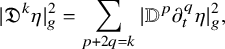
 $$ \begin{align} \mathfrak{D}^k\eta:=\sum_{p+2q=k}{\mathbb{D}}^p \partial_t^q \eta, \end{align} $$
which is a sum of tensors of different types. We will also use the notation
 $$ \begin{align} \mathfrak{D}^k_{\mathbf{bt}}\eta:=\sum_{p+2q=k}{\mathbb{D}}^p_{\mathbf{b}\cdots\mathbf{b}} \partial_t^q \eta \end{align} $$
when we only take spatial base derivatives, as well as time derivatives. Observe also that if g is any Riemannian product metric on
 $B\times Y$
, then we have the pointwise equality
$B\times Y$
, then we have the pointwise equality
 $$ \begin{align} |\mathfrak{D}^k\eta|^2_g=\sum_{p+2q=k}|{\mathbb{D}}^p \partial_t^q \eta|^2_g, \end{align} $$
which we will use implicitly many times.
In our setting,
 $\{g_{Y,z}\}_{z\in B},$
is a smooth family of Riemannian metrics on Y, so (up to shrinking B slightly) we can find
$\{g_{Y,z}\}_{z\in B},$
is a smooth family of Riemannian metrics on Y, so (up to shrinking B slightly) we can find
 $\Lambda>1$
so that
$\Lambda>1$
so that
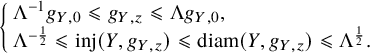 $$ \begin{align} \left\{ \begin{array}{ll} \Lambda^{-1} g_{Y,0}\leqslant g_{Y,z}\leqslant \Lambda g_{Y,0},\\ \Lambda^{-\frac{1}{2}} \leqslant \mathrm{inj}(Y,g_{Y,z}) \leqslant \mathrm{diam}(Y,g_{Y,z})\leqslant \Lambda^{\frac{1}{2}}. \end{array} \right. \end{align} $$
In particular, the norm measured with respect to
 $g_{Y,0}$
is uniformly comparable to that of
$g_{Y,0}$
is uniformly comparable to that of
 $g_{Y,z}$
for
$g_{Y,z}$
for
 $z\in B$
.
$z\in B$
.
2.3 Hölder seminorms
We now use the connection
 ${\mathbb {D}}$
to define a parabolic Hölder norm on
${\mathbb {D}}$
to define a parabolic Hölder norm on
 $B\times Y\times [0,+\infty )$
. For
$B\times Y\times [0,+\infty )$
. For
 $p=(z,y)\in B\times Y,t\geqslant 0, 0<R\leqslant \sqrt {t}$
and (shrinking) product metrics
$p=(z,y)\in B\times Y,t\geqslant 0, 0<R\leqslant \sqrt {t}$
and (shrinking) product metrics
 $g_\zeta (\tau )=g_{\mathbb {C}^m}+e^{-\tau } g_{Y,\zeta }$
, we define the parabolic domain
$g_\zeta (\tau )=g_{\mathbb {C}^m}+e^{-\tau } g_{Y,\zeta }$
, we define the parabolic domain
 $$ \begin{align} Q_{g_\zeta(\tau),R}(p,t)= B_{\mathbb{C}^m}(z,R)\times B_{e^{-\tau}g_{Y,\zeta}}(y,R)\times [t-R^2,t]. \end{align} $$
The parabolic domain with respect to any other product metric is defined analogously. We will very often simply take
 $\zeta =0\in B$
.
$\zeta =0\in B$
.
Definition 2.2. For any
 $0<{\alpha }<1$
,
$0<{\alpha }<1$
,
 $R>0$
,
$R>0$
,
 $p\in B\times Y$
,
$p\in B\times Y$
,
 $t\geqslant 0$
and smooth tensor field
$t\geqslant 0$
and smooth tensor field
 $\eta $
on
$\eta $
on
 $B\times Y\times [t-R^2,t]$
, given a product metric g (such as
$B\times Y\times [t-R^2,t]$
, given a product metric g (such as
 $g=g_z(\tau )$
for some
$g=g_z(\tau )$
for some
 $z\in B$
and
$z\in B$
and
 $\tau \geqslant 0$
), we define
$\tau \geqslant 0$
), we define
 $$ \begin{align} [\eta]_{{\alpha},{\alpha}/2, Q_{g,R}(p,t),g}=\sup \left\{ \frac{|\eta(x,s)-\mathbb{P}_{x'x}\eta(x',s')|_g}{(d^g(x,x')+|s-s'|^{\frac{1}{2}})^{\alpha}}\right\}, \end{align} $$
where the supremum is taken among all
 $(x,s)$
and
$(x,s)$
and
 $(x',s')$
in
$(x',s')$
in
 $Q_{g,R}(p,t)$
in which x and
$Q_{g,R}(p,t)$
in which x and
 $x'$
are either horizontally or vertically joined by a
$x'$
are either horizontally or vertically joined by a
 $\mathbb {P}$
-geodesic.
$\mathbb {P}$
-geodesic.
In the case when we use
 $g=g_z(\tau )$
and
$g=g_z(\tau )$
and
 $\tau $
is allowed to go to
$\tau $
is allowed to go to
 $+\infty $
, we will refer to these as shrinking parabolic Hölder seminorms. Nevertheless, for each fixed
$+\infty $
, we will refer to these as shrinking parabolic Hölder seminorms. Nevertheless, for each fixed
 $R>0$
, we will have
$R>0$
, we will have
 $$ \begin{align} B_{\mathbb{C}^m}(z,R)\times B_{e^{-\tau}g_{Y,z}}(y,R)=B_{\mathbb{C}^m}(z,R)\times Y \end{align} $$
for all
 $\tau>\tau _0(R,Y)$
. This will be the setting where the parabolic Hölder seminorm are applied in the whole paper. In this case, we will simply denote it by
$\tau>\tau _0(R,Y)$
. This will be the setting where the parabolic Hölder seminorm are applied in the whole paper. In this case, we will simply denote it by
 $$ \begin{align} Q_R(z,t)=B_{\mathbb{C}^m}(z,R)\times Y \times [t-R^2,t] \end{align} $$
when the metric g and the shrinking rate
 $\tau $
play no role.
$\tau $
play no role.
Lastly, as in [Reference Hein and Tosatti21, (4.101)], it will also be useful to consider (shrinking) parabolic Hölder seminorms
 $[\eta ]_{{\alpha },{\alpha }/2,\mathrm {base}, Q_{g,R}(p,t),g}$
which are defined as in (2.7) but where the supremum is taken only among
$[\eta ]_{{\alpha },{\alpha }/2,\mathrm {base}, Q_{g,R}(p,t),g}$
which are defined as in (2.7) but where the supremum is taken only among
 $(x,s)$
and
$(x,s)$
and
 $(x',s')$
in
$(x',s')$
in
 $Q_{g,R}(p,t)$
such that x and
$Q_{g,R}(p,t)$
such that x and
 $x'$
are horizontally joined by a
$x'$
are horizontally joined by a
 $\mathbb {P}$
-geodesic.
$\mathbb {P}$
-geodesic.
2.4 Parabolic interpolation
We need an interpolation inequality between the highest order (i.e.,
 $C^{k+{\alpha },(k+{\alpha })/2}$
) and the lowest order (i.e.,
$C^{k+{\alpha },(k+{\alpha })/2}$
) and the lowest order (i.e.,
 $L^\infty $
) norms of a tensor. In the parabolic framework, it will be more convenient to interpolate with the top even order (cf. Remark 2.5). This can be viewed as a parabolic version of [Reference Hein and Tosatti21, Proposition 2.8], and as in there it is crucial that the constants in the interpolation inequality are independent of the shrinking size parameter
$L^\infty $
) norms of a tensor. In the parabolic framework, it will be more convenient to interpolate with the top even order (cf. Remark 2.5). This can be viewed as a parabolic version of [Reference Hein and Tosatti21, Proposition 2.8], and as in there it is crucial that the constants in the interpolation inequality are independent of the shrinking size parameter
 $\tau \geqslant 0$
.
$\tau \geqslant 0$
.
Proposition 2.3. For any
 $k\in \mathbb {N}_{>0}$
and
$k\in \mathbb {N}_{>0}$
and
 ${\alpha }\in (0,1)$
, there exists
${\alpha }\in (0,1)$
, there exists
 $C_k=C_k({\alpha },\Lambda )>0$
(where
$C_k=C_k({\alpha },\Lambda )>0$
(where
 $\Lambda $
is given in (2.5)) such that the following holds. Let
$\Lambda $
is given in (2.5)) such that the following holds. Let
 $\eta $
be a smooth contravariant p-tensor on
$\eta $
be a smooth contravariant p-tensor on
 $B\times Y$
. Then for all
$B\times Y$
. Then for all
 $(x_0, t_0)\in B\times Y\times \mathbb {R}$
,
$(x_0, t_0)\in B\times Y\times \mathbb {R}$
,
 $ 0<\rho <R$
and
$ 0<\rho <R$
and
 $\tau \geqslant 0$
such that
$\tau \geqslant 0$
such that
 $ Q_{g_0(\tau ),R}(x_0,t_0)\Subset B\times Y\times \mathbb {R}$
, we have
$ Q_{g_0(\tau ),R}(x_0,t_0)\Subset B\times Y\times \mathbb {R}$
, we have
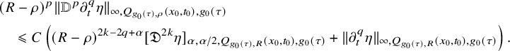
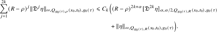 $$ \begin{align} \begin{aligned} \sum_{j=1}^{2k}(R-\rho)^{j} \| \mathfrak{D}^j \eta \|_{\infty, Q_{g_0(\tau),\rho}(x_0,t_0),g_0(\tau)}&\leqslant C_k\Big((R-\rho)^{2k+{\alpha}}[\mathfrak{D}^{2k} \eta] _{{\alpha},{\alpha}/2, Q_{g_0(\tau),R}(x_0,t_0),g_0(\tau)}\\&\quad\quad \;\;+\| \eta \|_{\infty, Q_{g_0(\tau),R}(x_0,t_0),g_0(\tau)}\Big). \end{aligned} \end{align} $$
Moreover, for any
 $j\in \mathbb {N}$
and
$j\in \mathbb {N}$
and
 ${\beta }\in (0,1)$
with
${\beta }\in (0,1)$
with
 $j+{\beta }<2k+{\alpha }$
, we have
$j+{\beta }<2k+{\alpha }$
, we have
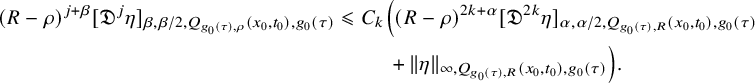 $$ \begin{align} \begin{aligned} (R-\rho)^{j+{\beta}} [\mathfrak{D}^j \eta ]_{{\beta},{\beta}/2, Q_{g_0(\tau),\rho}(x_0,t_0),g_0(\tau)}&\leqslant C_k\Big((R-\rho)^{2k+{\alpha}}[\mathfrak{D}^{2k} \eta] _{{\alpha},{\alpha}/2, Q_{g_0(\tau),R}(x_0,t_0),g_0(\tau)}\\&\quad\quad \;\;+\| \eta \|_{\infty, Q_{g_0(\tau),R}(x_0,t_0),g_0(\tau)}\Big). \end{aligned} \end{align} $$
Proof. We first show (2.10). Fix a pair of
 $(p,q)$
such that
$(p,q)$
such that
 $0<j=p+2q\leqslant 2k$
, and assume first that
$0<j=p+2q\leqslant 2k$
, and assume first that
 $p>0$
. Since
$p>0$
. Since
 $d^{g_0(\tau )}(x,x_0)<\rho $
for
$d^{g_0(\tau )}(x,x_0)<\rho $
for
 $(x,t)\in Q_{g_0(\tau ),\rho }(x_0,t_0)$
, we can treat
$(x,t)\in Q_{g_0(\tau ),\rho }(x_0,t_0)$
, we can treat
 $\partial _t^q \eta |_{(x,t)}$
as a smooth tensor on
$\partial _t^q \eta |_{(x,t)}$
as a smooth tensor on
 $B_{\mathbb {C}^m}(z_0,\rho )\times Y$
by freezing t so that [Reference Hein and Tosatti21, Proposition 2.8] applies to conclude
$B_{\mathbb {C}^m}(z_0,\rho )\times Y$
by freezing t so that [Reference Hein and Tosatti21, Proposition 2.8] applies to conclude
 $$ \begin{align} \begin{aligned} &(R-\rho)^{p}\| {\mathbb{D}}^p \partial_t^q \eta \|_{\infty, Q_{g_0(\tau),\rho}(x_0,t_0),g_0(\tau)}\\& \quad \leqslant C \left((R-\rho)^{2k-2q+{\alpha}} [\mathfrak{D}^{2k} \eta] _{{\alpha},{\alpha}/2, Q_{g_0(\tau),R}(x_0,t_0),g_0(\tau)} +\| \partial_t^q\eta \|_{\infty, Q_{g_0(\tau),R}(x_0,t_0),g_0(\tau)} \right). \end{aligned} \end{align} $$
Thus, it remains to show the interpolation on time derivatives (i.e., we assume in the rest that
 $p=0$
, so
$p=0$
, so
 $q>0$
). For each
$q>0$
). For each
 $(x,t)\in Q_{g_0(\tau ),\rho }(x_0,t_0)$
, fix
$(x,t)\in Q_{g_0(\tau ),\rho }(x_0,t_0)$
, fix
 $s=(R-\rho )^2>0$
so that
$s=(R-\rho )^2>0$
so that
 $(x,t-s)\in Q_{g_0(\tau ),R}(x_0,t_0)$
. Then there exists
$(x,t-s)\in Q_{g_0(\tau ),R}(x_0,t_0)$
. Then there exists
 $t_s\in [t-s,t]$
so that
$t_s\in [t-s,t]$
so that
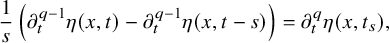 $$ \begin{align} \frac{1}{s}\left(\partial_t^{q-1}\eta(x,t)-\partial_t^{q-1}\eta(x,t-s)\right)=\partial_t^{q} \eta(x,t_s), \end{align} $$
which allows us to estimate
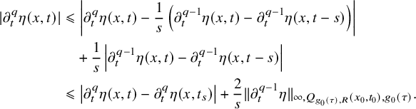 $$ \begin{align} \begin{aligned} |\partial_t^q\eta (x,t)|&\leqslant \left|\partial_t^q\eta (x,t)-\frac1s\left(\partial_t^{q-1}\eta(x,t)-\partial_t^{q-1}\eta(x,t-s) \right) \right|\\ &\quad +\frac1s \left|\partial_t^{q-1}\eta(x,t)-\partial_t^{q-1}\eta(x,t-s) \right|\\ &\leqslant \left|\partial_t^{q}\eta (x,t)-\partial_t^{q} \eta(x,t_s) \right|+ \frac2s \|\partial_t^{q-1} \eta \|_{\infty, Q_{g_0(\tau),R}(x_0,t_0),g_0(\tau)}. \end{aligned} \end{align} $$
If
 $q=k$
, we arrive at
$q=k$
, we arrive at
 $$ \begin{align*} \begin{aligned} \| \partial_t^k \eta \|_{\infty, Q_{g_0(\tau),\rho}(x_0,t_0),g_0(\tau)}&\leqslant (R-\rho)^{{\alpha}}[\partial_t^k \eta]_{{\alpha},{\alpha}/2, Q_{g_0(\tau),R}(x_0,t_0),g_0(\tau)} \\ &\quad + \frac2{(R-\rho)^2} \|\partial_t^{k-1} \eta \|_{\infty, Q_{g_0(\tau),R}(x_0,t_0),g_0(\tau)}. \end{aligned} \end{align*} $$
Otherwise,
 $q<k$
, and we have
$q<k$
, and we have
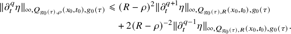 $$ \begin{align*} \begin{aligned} \| \partial_t^q \eta \|_{\infty, Q_{g_0(\tau),\rho}(x_0,t_0),g_0(\tau)}&\leqslant (R-\rho)^{2}\|\partial_t^{q+1} \eta\|_{\infty, Q_{g_0(\tau),R}(x_0,t_0),g_0(\tau)} \\ &\quad +2(R-\rho)^{-2} \|\partial_t^{q-1} \eta \|_{\infty, Q_{g_0(\tau),R}(x_0,t_0),g_0(\tau)}. \end{aligned} \end{align*} $$
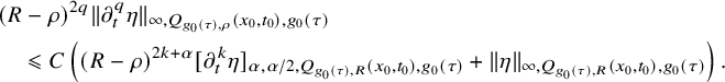
Applying this dichotomy inductively, with suitable replacements of
 $\rho $
and R at each step, we conclude that there exists
$\rho $
and R at each step, we conclude that there exists
 $C>0$
so that for each
$C>0$
so that for each
 $1\leqslant q\leqslant k$
,
$1\leqslant q\leqslant k$
,
 $$ \begin{align} \begin{aligned} &(R-\rho)^{2q}\| \partial_t^q \eta \|_{\infty, Q_{g_0(\tau),\rho}(x_0,t_0),g_0(\tau)}\\&\quad \leqslant C \left((R-\rho)^{2k+{\alpha}} [\partial_t^k \eta] _{{\alpha},{\alpha}/2, Q_{g_0(\tau),R}(x_0,t_0),g_0(\tau)} +\|\eta \|_{\infty, Q_{g_0(\tau),R}(x_0,t_0),g_0(\tau)} \right). \end{aligned} \end{align} $$
By combining this with (2.12), we see that (2.10) follows.
It remains to prove (2.11). Fix
 $(x,t),(x',s)\in Q_{g_0(\tau ),\rho }(x_0,t_0)$
such that x and
$(x,t),(x',s)\in Q_{g_0(\tau ),\rho }(x_0,t_0)$
such that x and
 $x'$
are joined either horizontally or vertically by a
$x'$
are joined either horizontally or vertically by a
 $\mathbb {P}$
-geodesic. Denote
$\mathbb {P}$
-geodesic. Denote
 $d=d^{g_0(\tau )}(x,x')+|t-s|^{\frac {1}{2}}$
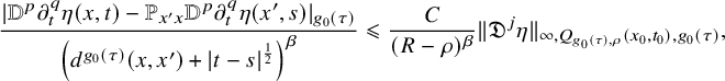
. We want to estimate
$d=d^{g_0(\tau )}(x,x')+|t-s|^{\frac {1}{2}}$
. We want to estimate
 $|\mathfrak {D}^j \eta (x,t)-\mathbb {P}_{x'x} \mathfrak {D}^j\eta (x',s)|_{g_0(\tau )}$
. Fix a pair of
$|\mathfrak {D}^j \eta (x,t)-\mathbb {P}_{x'x} \mathfrak {D}^j\eta (x',s)|_{g_0(\tau )}$
. Fix a pair of
 $(p,q)$
such that
$(p,q)$
such that
 $0<p+2q=j\leqslant 2k$
and
$0<p+2q=j\leqslant 2k$
and
 ${\beta }\in (0,1)$
with
${\beta }\in (0,1)$
with
 $j+\beta <2k+\alpha $
.
$j+\beta <2k+\alpha $
.
If
 $d\geqslant \frac 1{4\Lambda } (R-\rho )$
where
$d\geqslant \frac 1{4\Lambda } (R-\rho )$
where
 $\Lambda $
is the constant in (2.5), then using the triangle inequality and the boundedness of the operator norm of
$\Lambda $
is the constant in (2.5), then using the triangle inequality and the boundedness of the operator norm of
 $\mathbb {P}$
from [Reference Hein and Tosatti21, §2.1.1], we deduce that
$\mathbb {P}$
from [Reference Hein and Tosatti21, §2.1.1], we deduce that
 $$ \begin{align} \begin{aligned} \frac{|{\mathbb{D}}^p\partial_t^q \eta(x,t)-\mathbb{P}_{x'x} {\mathbb{D}}^p\partial_t^q\eta(x',s)|_{g_0(\tau)}}{\left(d^{g_0(\tau)}(x,x')+|t-s|^{\frac{1}{2}} \right)^{\beta}}&\leqslant \frac{C}{(R-\rho)^{\beta}} \| \mathfrak{D}^j \eta \|_{\infty, Q_{g_0(\tau),\rho}(x_0,t_0),g_0(\tau)}, \end{aligned} \end{align} $$
so that the conclusion follows from (2.10).
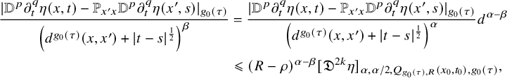
If
 $d<\frac 1{4\Lambda } (R-\rho )$
,
$d<\frac 1{4\Lambda } (R-\rho )$
,
 $j=2k$
and
$j=2k$
and
 ${\beta }<{\alpha }$
, then
${\beta }<{\alpha }$
, then
 $$ \begin{align} \begin{aligned} \frac{|{\mathbb{D}}^p\partial_t^q \eta(x,t)-\mathbb{P}_{x'x} {\mathbb{D}}^p\partial_t^q\eta(x',s)|_{g_0(\tau)}}{\left(d^{g_0(\tau)}(x,x')+|t-s|^{\frac{1}{2}} \right)^{\beta}}&=\frac{|{\mathbb{D}}^p\partial_t^q \eta(x,t)-\mathbb{P}_{x'x} {\mathbb{D}}^p\partial_t^q\eta(x',s)|_{g_0(\tau)}}{\left(d^{g_0(\tau)}(x,x')+|t-s|^{\frac{1}{2}} \right)^{\alpha}} d^{{\alpha}-{\beta}}\\ &\leqslant (R-\rho)^{{\alpha}-{\beta}}[\mathfrak{D}^{2k} \eta] _{{\alpha},{\alpha}/2, Q_{g_0(\tau),R}(x_0,t_0),g_0(\tau)}, \end{aligned} \end{align} $$
which is acceptable. It remains to consider the case when
 $d<\frac 1{4\Lambda } (R-\rho )$
and
$d<\frac 1{4\Lambda } (R-\rho )$
and
 $j=p+2q<2k$
. Here, using again the boundedness of
$j=p+2q<2k$
. Here, using again the boundedness of
 $\mathbb {P}$
, we can estimate
$\mathbb {P}$
, we can estimate
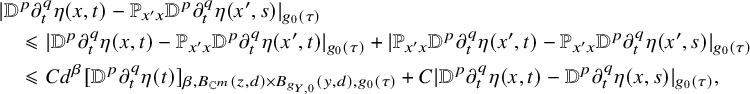 $$ \begin{align} \begin{aligned} &|{\mathbb{D}}^p\partial_t^q \eta(x,t)-\mathbb{P}_{x'x} {\mathbb{D}}^p\partial_t^q\eta(x',s)|_{g_0(\tau)}\\&\quad\leqslant |{\mathbb{D}}^p\partial_t^q \eta(x,t)-\mathbb{P}_{x'x} {\mathbb{D}}^p\partial_t^q\eta(x',t)|_{g_0(\tau)}+|\mathbb{P}_{x'x} {\mathbb{D}}^p\partial_t^q\eta(x',t)-\mathbb{P}_{x'x} {\mathbb{D}}^p\partial_t^q\eta(x',s)|_{g_0(\tau)}\\&\quad\leqslant Cd^{\beta} [{\mathbb{D}}^p\partial_t^q \eta(t)]_{{\beta}, B_{\mathbb{C}^m}(z,d)\times B_{g_{Y,0}}(y,d),g_0(\tau)} +C| {\mathbb{D}}^p\partial_t^q\eta(x,t)-{\mathbb{D}}^p\partial_t^q\eta(x,s)|_{g_0(\tau)}, \end{aligned} \end{align} $$
where the first term is the spatial Hölder seminorm of the tensor
 $\partial _t^q\eta (t)$
with t frozen, and
$\partial _t^q\eta (t)$
with t frozen, and
 $x=(z,y)\in \mathbb {C}^m\times Y$
. Applying [Reference Hein and Tosatti21, Lemma 2.5] to the first term in the last line of (2.18) gives
$x=(z,y)\in \mathbb {C}^m\times Y$
. Applying [Reference Hein and Tosatti21, Lemma 2.5] to the first term in the last line of (2.18) gives
 $$ \begin{align}\begin{aligned} [{\mathbb{D}}^p\partial_t^q \eta(t)]_{{\beta}, B_{\mathbb{C}^m}(z,d)\times B_{g_{Y,0}}(y,d),g_0(\tau)} &\leqslant C d^{1-{\beta}} \| {\mathbb{D}}^{p+1} \partial_t^q\eta(t)\|_{\infty, B_{\mathbb{C}^m}(z,d)\times B_{g_{Y,0}}(y,d),g_0(\tau)}\\ &\leqslant C d^{1-{\beta}} \| \mathfrak{D}^{j+1} \eta\|_{\infty, Q_{g_0(\tau),R}(x_0,t_0),g_0(\tau)}. \end{aligned} \end{align} $$
As for the second term in the last line of (2.18), assume first that
 $j+2=p+2(q+1)\leqslant 2k$
. In this case, we can argue similarly by estimating the difference in term of time derivatives
$j+2=p+2(q+1)\leqslant 2k$
. In this case, we can argue similarly by estimating the difference in term of time derivatives
 $$ \begin{align} | {\mathbb{D}}^p\partial_t^q\eta(x,t)-{\mathbb{D}}^p\partial_t^q\eta(x,s)|_{g_0(\tau)}\leqslant d^2 \| \mathfrak{D}^{j+2} \eta\|_{\infty, Q_{g_0(\tau),R}(x_0,t_0),g_0(\tau)}. \end{align} $$
Hence, under the assumption that
 $j+2=p+2(q+1)\leqslant 2k$
, we can combine (2.18), (2.19) and (2.20) to get
$j+2=p+2(q+1)\leqslant 2k$
, we can combine (2.18), (2.19) and (2.20) to get
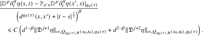 $$ \begin{align} \begin{aligned} &\frac{|{\mathbb{D}}^p\partial_t^q \eta(x,t)-\mathbb{P}_{x'x} {\mathbb{D}}^p\partial_t^q\eta(x',s)|_{g_0(\tau)}}{\left(d^{g_0(\tau)}(x,x')+|t-s|^{\frac{1}{2}} \right)^{\beta}}\\&\quad \leqslant C \left(d^{1-{\beta}} \| \mathfrak{D}^{j+1} \eta\|_{\infty, Q_{g_0(\tau),R}(x_0,t_0),g_0(\tau)}+ d^{2-{\beta}}\| \mathfrak{D}^{j+2} \eta\|_{\infty, Q_{g_0(\tau),R}(x_0,t_0),g_0(\tau)} \right). \end{aligned} \end{align} $$
The conclusion then follows by combining with (2.10) since
 $d\leqslant \frac 1{4\Lambda }(R-\rho )$
.
$d\leqslant \frac 1{4\Lambda }(R-\rho )$
.
It remains to consider the case when
 $p+2q<2k<p+2q+2$
(i.e.,
$p+2q<2k<p+2q+2$
(i.e.,
 $p+2q=2k-1$
). This implies that p is odd, and hence,
$p+2q=2k-1$
). This implies that p is odd, and hence,
 $p\geqslant 1$
. Let v run over a
$p\geqslant 1$
. Let v run over a
 $g_0(\tau )$
-orthonormal basis of tangent vectors which are either horizontal or vertical. Let
$g_0(\tau )$
-orthonormal basis of tangent vectors which are either horizontal or vertical. Let
 $\gamma (u)$
be the unique
$\gamma (u)$
be the unique
 $\mathbb {P}$
-geodesic with
$\mathbb {P}$
-geodesic with
 $\gamma (0)=x$
and
$\gamma (0)=x$
and
 $\dot \gamma (0)=v$
with
$\dot \gamma (0)=v$
with
 $u\in (0,R-\rho )$
. Denote
$u\in (0,R-\rho )$
. Denote
 $\sigma (u,\cdot )=\mathbb {P}^{-1}_{\gamma (0),\gamma (u)}{\mathbb {D}}^{p-1}\partial _t^{q} \eta (\gamma (u),\cdot )$
so that
$\sigma (u,\cdot )=\mathbb {P}^{-1}_{\gamma (0),\gamma (u)}{\mathbb {D}}^{p-1}\partial _t^{q} \eta (\gamma (u),\cdot )$
so that
 ${\mathbb {D}}_v {\mathbb {D}}^{p-1}\partial _t^{q}\eta (x,\cdot )=\partial _u|_{u=0}\sigma (u,\cdot )$
. By the mean value theorem, there exists
${\mathbb {D}}_v {\mathbb {D}}^{p-1}\partial _t^{q}\eta (x,\cdot )=\partial _u|_{u=0}\sigma (u,\cdot )$
. By the mean value theorem, there exists
 $\theta \in [0,1]$
such that
$\theta \in [0,1]$
such that
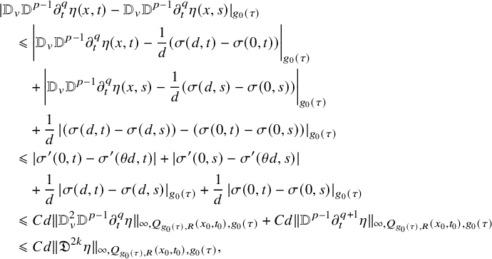 $$ \begin{align} \begin{aligned} &| {\mathbb{D}}_v {\mathbb{D}}^{p-1}\partial_t^{q}\eta(x,t)-{\mathbb{D}}_v{\mathbb{D}}^{p-1}\partial_t^{q}\eta(x,s)|_{g_0(\tau)}\\&\quad\leqslant \left| {\mathbb{D}}_v {\mathbb{D}}^{p-1}\partial_t^{q}\eta(x,t)-\frac1d( \sigma(d,t)- \sigma(0,t))\right|_{g_0(\tau)}\\&\qquad +\left| {\mathbb{D}}_v {\mathbb{D}}^{p-1}\partial_t^{q}\eta(x,s)-\frac1d( \sigma(d,s)- \sigma(0,s))\right|_{g_0(\tau)}\\&\qquad +\frac1d \left| ( \sigma(d,t)- \sigma(d,s))-( \sigma(0,t)- \sigma(0,s))\right|_{g_0(\tau)}\\&\quad\leqslant |\sigma'(0,t)-\sigma'(\theta d,t)|+ |\sigma'(0,s)-\sigma'(\theta d,s)| \\&\qquad +\frac1d \left|\sigma(d,t)- \sigma(d,s)\right|_{g_0(\tau)}+\frac1d \left|\sigma(0,t)- \sigma(0,s)\right|_{g_0(\tau)}\\&\quad\leqslant C d \|{\mathbb{D}}^2_v {\mathbb{D}}^{p-1}\partial_t^{q} \eta\|_{\infty, Q_{g_0(\tau),R}(x_0,t_0),g_0(\tau)}+ C d \| {\mathbb{D}}^{p-1}\partial_t^{q+1} \eta\|_{\infty, Q_{g_0(\tau),R}(x_0,t_0),g_0(\tau)}\\&\quad\leqslant C d\|\mathfrak{D}^{2k} \eta\| _{\infty, Q_{g_0(\tau),R}(x_0,t_0),g_0(\tau)}, \end{aligned} \end{align} $$
where
 $\sigma '$
denotes the u-derivative. Since v is arbitrary, we conclude that
$\sigma '$
denotes the u-derivative. Since v is arbitrary, we conclude that
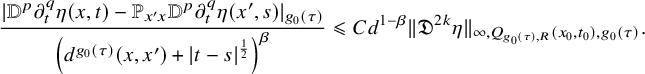 $$ \begin{align} \frac{|{\mathbb{D}}^p\partial_t^{q} \eta(x,t)-\mathbb{P}_{x'x} {\mathbb{D}}^{p}\partial_t^{q}\eta(x',s)|_{g_0(\tau)}}{\left(d^{g_0(\tau)}(x,x')+|t-s|^{\frac{1}{2}} \right)^{\beta}} \leqslant C d^{1-{\beta}}\|\mathfrak{D}^{2k} \eta\| _{\infty, Q_{g_0(\tau),R}(x_0,t_0),g_0(\tau)}. \end{align} $$
The result then follows using (2.10) again. This completes the proof.
We end this subsection by showing that a function on
 $\mathbb {R}^n\times (-\infty ,0]$
with bounded
$\mathbb {R}^n\times (-\infty ,0]$
with bounded
 $(2k+{\alpha })$
parabolic Hölder seminorm and vanishing parabolic
$(2k+{\alpha })$
parabolic Hölder seminorm and vanishing parabolic
 $2k$
jet at
$2k$
jet at
 $(x,t)=(0,0)$
will be bounded in
$(x,t)=(0,0)$
will be bounded in
 $C^{2k+{\alpha },k+{\alpha }/2}_{\mathrm {loc}}$
.
$C^{2k+{\alpha },k+{\alpha }/2}_{\mathrm {loc}}$
.
Lemma 2.4. Let u be a smooth function on
 $\mathbb {R}^n\times (-\infty ,0]$
such that
$\mathbb {R}^n\times (-\infty ,0]$
such that
 $$ \begin{align} [\mathfrak{D}^{2k}u]_{{\alpha},{\alpha}/2,B_{\mathbb{R}^n}(R)\times [-R^2,0]}\leqslant \Lambda_0 \end{align} $$
for some
 $R,\Lambda _0>0,k\in \mathbb {N}$
and
$R,\Lambda _0>0,k\in \mathbb {N}$
and
 $\mathfrak {D}^{\ell }u|_{(0,0)}=0$
for all
$\mathfrak {D}^{\ell }u|_{(0,0)}=0$
for all
 $0\leqslant \ell \leqslant 2k$
. Then for all
$0\leqslant \ell \leqslant 2k$
. Then for all
 $0<r\leqslant R$
and
$0<r\leqslant R$
and
 $0\leqslant m\leqslant 2k$
, there exists
$0\leqslant m\leqslant 2k$
, there exists
 $C_0(n,m)>0$
such that
$C_0(n,m)>0$
such that
 $$ \begin{align} \|\mathfrak{D}^{m}u\|_{\infty,B_{\mathbb{R}^n}(r)\times [-r^2,0]}\leqslant C_0\Lambda_0 r^{2k+{\alpha}-m}.\end{align} $$
Moreover, for all
 ${\beta }\in (0,{\alpha })$
, there exists
${\beta }\in (0,{\alpha })$
, there exists
 $C_1(n,\Lambda _0,{\beta })>0$
such that
$C_1(n,\Lambda _0,{\beta })>0$
such that
 $$ \begin{align} [\mathfrak{D}^{m}u]_{{\beta},{\beta}/2,B_{\mathbb{R}^n}(r)\times [-r^2,0]}\leqslant C_1\Lambda_0 r^{2k+{\alpha}-m-{\beta}}.\end{align} $$
Remark 2.5. This Lemma is false as stated if we replace
 $2k$
with an odd integer, and this is the main reason why in our main Theorem 4.2, we will restrict to even order derivatives. The simplest counterexample is the function
$2k$
with an odd integer, and this is the main reason why in our main Theorem 4.2, we will restrict to even order derivatives. The simplest counterexample is the function
 $u(x,t)=t$
in
$u(x,t)=t$
in
 $\mathbb {R}\times \mathbb {R}$
, which satisfies
$\mathbb {R}\times \mathbb {R}$
, which satisfies
 $u(0,0)=0$
,
$u(0,0)=0$
,
 $\mathfrak {D} u|_{(0,0)}=0$
and
$\mathfrak {D} u|_{(0,0)}=0$
and
 $[\mathfrak {D} u]_{{\alpha },{\alpha }/2,\mathbb {R}\times \mathbb {R}}=0$
but (2.25) fails for
$[\mathfrak {D} u]_{{\alpha },{\alpha }/2,\mathbb {R}\times \mathbb {R}}=0$
but (2.25) fails for
 $m=0$
.
$m=0$
.
To fix this, one has to redefine the parabolic Hölder seminorms of odd order by adding an additional term; see [Reference Lieberman29, p.46]. If one were to do this, then the statement of Lemma 2.4 would also hold when
 $2k$
is replaced by an odd integer. However, the additional term that one would need to add would not be compatible with our blowup arguments in section 4, especially with the ‘non-escaping property’ in Section 4.5.
$2k$
is replaced by an odd integer. However, the additional term that one would need to add would not be compatible with our blowup arguments in section 4, especially with the ‘non-escaping property’ in Section 4.5.
Proof. Write
 $Q_r=B_{\mathbb {R}^n}(r)\times [-r^2,0]$
for notational convenience. We only prove the bound for
$Q_r=B_{\mathbb {R}^n}(r)\times [-r^2,0]$
for notational convenience. We only prove the bound for
 $\|\mathfrak {D}^m u\|_{\infty }$
in (2.25) since the bound for Hölder seminorm in (2.26) is similar.
$\|\mathfrak {D}^m u\|_{\infty }$
in (2.25) since the bound for Hölder seminorm in (2.26) is similar.
By considering
 $\tilde u(x,t)=\Lambda _0 ^{-1}R^{-2k-{\alpha }}u(Rx,R^2t)$
for
$\tilde u(x,t)=\Lambda _0 ^{-1}R^{-2k-{\alpha }}u(Rx,R^2t)$
for
 $(x,t)\in B_{\mathbb {R}^n}(1)\times [-1,0]$
, we can assume
$(x,t)\in B_{\mathbb {R}^n}(1)\times [-1,0]$
, we can assume
 $\Lambda _0=1=R=1$
and
$\Lambda _0=1=R=1$
and
 $0<r\leqslant 1$
. We prove the result by induction on k. In case
$0<r\leqslant 1$
. We prove the result by induction on k. In case
 $k=0$
, the jet assumption is equivalent to
$k=0$
, the jet assumption is equivalent to
 $u(0,0)=0$
, and hence for all
$u(0,0)=0$
, and hence for all
 $0<r\leqslant 1$
,
$0<r\leqslant 1$
,
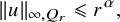 $$ \begin{align} \|u\|_{\infty,Q_r}\leqslant r^{\alpha}, \end{align} $$
so that the conclusion holds.
Next, we consider the induction step, so we assume that the conclusion holds for all
 $0\leqslant \ell \leqslant k$
and prove it for
$0\leqslant \ell \leqslant k$
and prove it for
 $k+1\geqslant 1$
. Given a smooth function u with
$k+1\geqslant 1$
. Given a smooth function u with
 $[\mathfrak {D}^{2k+2}u]_{{\alpha },{\alpha }/2,Q_1}\leqslant 1$
, given any
$[\mathfrak {D}^{2k+2}u]_{{\alpha },{\alpha }/2,Q_1}\leqslant 1$
, given any
 $0\leqslant m\leqslant 2k$
, every derivative
$0\leqslant m\leqslant 2k$
, every derivative
 $\mathfrak {D}^{m+2}u$
can be written as
$\mathfrak {D}^{m+2}u$
can be written as
 $\mathfrak {D}^m v$
where
$\mathfrak {D}^m v$
where
 $v=\partial _t u$
or
$v=\partial _t u$
or
 $v={\mathbb {D}}^2 u$
(evaluated at some pair of tangent vectors). The function v satisfies
$v={\mathbb {D}}^2 u$
(evaluated at some pair of tangent vectors). The function v satisfies
 $[\mathfrak {D}^{2k}v]_{{\alpha },{\alpha }/2,Q_1}\leqslant 1$
and
$[\mathfrak {D}^{2k}v]_{{\alpha },{\alpha }/2,Q_1}\leqslant 1$
and
 $\mathfrak {D}^{\ell }v|_{(0,0)}=0$
for all
$\mathfrak {D}^{\ell }v|_{(0,0)}=0$
for all
 $0\leqslant \ell \leqslant 2k$
. The induction hypothesis then implies
$0\leqslant \ell \leqslant 2k$
. The induction hypothesis then implies
 $\|\mathfrak {D}^{m+2} u\|_{\infty ,Q_r}\leqslant C_{k} r^{2k+{\alpha }-m}$
for all
$\|\mathfrak {D}^{m+2} u\|_{\infty ,Q_r}\leqslant C_{k} r^{2k+{\alpha }-m}$
for all
 $0\leqslant m\leqslant 2k$
and
$0\leqslant m\leqslant 2k$
and
 $0<r\leqslant 1$
. It remains to extend it to
$0<r\leqslant 1$
. It remains to extend it to
 $m=-1,-2$
(i.e., to bound u and
$m=-1,-2$
(i.e., to bound u and
 ${\mathbb {D}} u$
). Let
${\mathbb {D}} u$
). Let
 $(x,t)\in Q_r$
and fix a unit vector
$(x,t)\in Q_r$
and fix a unit vector
 $e_1$
, and estimate
$e_1$
, and estimate
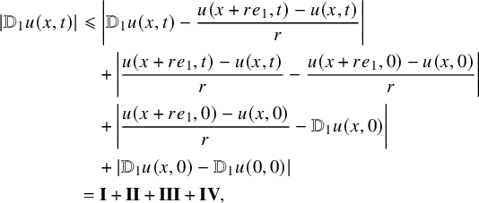 $$ \begin{align} \begin{aligned} |{\mathbb{D}}_1 u(x,t)|&\leqslant \left|{\mathbb{D}}_1 u(x,t)-\frac{u(x+re_1,t)-u(x,t)}{r}\right|\\ &\quad +\left|\frac{u(x+re_1,t)-u(x,t)}{r}-\frac{u(x+re_1,0)-u(x,0)}{r}\right|\\ &\quad +\left|\frac{u(x+re_1,0)-u(x,0)}{r}-{\mathbb{D}}_1u(x,0)\right|\\ &\quad +\left|{\mathbb{D}}_1u(x,0)-{\mathbb{D}}_1u(0,0)\right|\\ &=\mathbf{I}+\mathbf{II}+\mathbf{III}+\mathbf{IV}, \end{aligned} \end{align} $$
and we bound each of the numbered terms as follows. By the mean value theorem, there exists
 $\theta \in [0,1]$
such that
$\theta \in [0,1]$
such that
 $$ \begin{align} \mathbf{I}=\left|{\mathbb{D}}_1 u(x,t)-{\mathbb{D}}_1 u(x+\theta r e_1,t)\right|, \end{align} $$
and using [Reference Hein and Tosatti21, Lemma 2.5], we can bound this by
 $r\|\mathfrak {D}^2 u\|_{\infty ,Q_r}\leqslant C r^{2k+{\alpha }+1}.$
For the second term, the mean value theorem again shows that there is
$r\|\mathfrak {D}^2 u\|_{\infty ,Q_r}\leqslant C r^{2k+{\alpha }+1}.$
For the second term, the mean value theorem again shows that there is
 $\theta '\in [0,1]$
so that
$\theta '\in [0,1]$
so that
 $$ \begin{align} \begin{aligned} \mathbf{II}&=\frac{|t|}r \left|\partial_t u(x+re_1,\theta' t)- \partial_t u(x,\theta' t)\right|\leqslant r\|\partial_t u\|_{\infty, Q_r}\leqslant r\|\mathfrak{D}^2 u\|_{\infty,Q_r}\leqslant Cr^{2k+{\alpha}+1}. \end{aligned} \end{align} $$
For the third term, using the mean value theorem and [Reference Hein and Tosatti21, Lemma 2.5], we can find
 $\theta "\in [0,1]$
so that
$\theta "\in [0,1]$
so that
 $$ \begin{align} \begin{aligned} \mathbf{III}&=\left|{\mathbb{D}}_1 u(x+r\theta" e_1,0)-{\mathbb{D}}_1u(x,0)\right|\leqslant r\|{\mathbb{D}}^2 u\|_{\infty,Q_r}\leqslant r\|\mathfrak{D}^2 u\|_{\infty, Q_r}\leqslant Cr^{2k+{\alpha}+1}, \end{aligned} \end{align} $$
and for the fourth term, we again use [Reference Hein and Tosatti21, Lemma 2.5] to bound
 $$ \begin{align} \mathbf{IV}\leqslant r\|{\mathbb{D}}^2 u\|_{\infty,Q_r}\leqslant r\|\mathfrak{D}^2 u\|_{\infty, Q_r}\leqslant Cr^{2k+{\alpha}+1}, \end{align} $$
and putting these all together proves that
 $|{\mathbb {D}}_1 u(x,t)|\leqslant Cr^{2k+{\alpha }+1}$
, and hence,
$|{\mathbb {D}}_1 u(x,t)|\leqslant Cr^{2k+{\alpha }+1}$
, and hence,
 $\|\mathfrak {D} u\|_{\infty ,Q_r}\leqslant C_{k} r^{2k+{\alpha }+1}$
since
$\|\mathfrak {D} u\|_{\infty ,Q_r}\leqslant C_{k} r^{2k+{\alpha }+1}$
since
 $e_1$
is arbitrary. The upper bound for
$e_1$
is arbitrary. The upper bound for
 $|u|$
is now straightforward using the bounds on
$|u|$
is now straightforward using the bounds on
 ${\mathbb {D}} u$
and
${\mathbb {D}} u$
and
 $\partial _t u$
. This completes the proof of the inductive step.
$\partial _t u$
. This completes the proof of the inductive step.
2.5 Bounds on Hölder seminorms imply decay
In this section, we establish a generalization of [Reference Hein and Tosatti21, Theorem 2.11] to our setting. Recall that at each point
 $x=(z,y)\in B\times Y$
,
$x=(z,y)\in B\times Y$
,
 $\omega _{F,z}$
is the unique Kähler-Ricci flat metric on each fiber
$\omega _{F,z}$
is the unique Kähler-Ricci flat metric on each fiber
 $X_z$
which is cohomologous to
$X_z$
which is cohomologous to
 $\omega _0|_{X_z}$
. We can assume that
$\omega _0|_{X_z}$
. We can assume that
 $\int _{\{z\}\times Y} \omega _{F,z}^n=1$
for all
$\int _{\{z\}\times Y} \omega _{F,z}^n=1$
for all
 $z\in B$
. For any function f in space-time
$z\in B$
. For any function f in space-time
 $B\times Y\times \mathbb {R}$
, we will use
$B\times Y\times \mathbb {R}$
, we will use
 $\underline{f}(z,t)$
to denote its fiberwise average:
$\underline{f}(z,t)$
to denote its fiberwise average:
 $$ \begin{align} \underline{f}(z,t)=\int_{\{z\}\times Y} f(z,\cdot,t) \,\omega_{F,z}^n. \end{align} $$
The following result will be crucial for us:
Proposition 2.6. Suppose
 $g=g_{\mathbb {C}^m}+\delta ^2 g_{Y,0}$
is a metric on
$g=g_{\mathbb {C}^m}+\delta ^2 g_{Y,0}$
is a metric on
 $B\times Y$
, where
$B\times Y$
, where
 $0<\delta \leqslant 1$
is arbitrary. For any
$0<\delta \leqslant 1$
is arbitrary. For any
 $k\in \mathbb {N}, {\alpha }\in (0,1)$
and
$k\in \mathbb {N}, {\alpha }\in (0,1)$
and
 $0<\rho <R<1$
with
$0<\rho <R<1$
with
 $\rho \geqslant \Lambda \delta $
, there exists
$\rho \geqslant \Lambda \delta $
, there exists
 $C(k,{\alpha },\rho ,R)>0$
such that for all smooth function
$C(k,{\alpha },\rho ,R)>0$
such that for all smooth function
 $\varphi $
on
$\varphi $
on
 $B\times Y\times \mathbb {R}$
with
$B\times Y\times \mathbb {R}$
with
 $\underline{\varphi }=0$
,
$\underline{\varphi }=0$
,
 $x_0=(0,y_0), t_0\in \mathbb {R}$
and for all
$x_0=(0,y_0), t_0\in \mathbb {R}$
and for all
 $0\leqslant j\leqslant 2k$
, we have
$0\leqslant j\leqslant 2k$
, we have
 $$ \begin{align} \|\mathfrak{D}^j \varphi\|_{\infty,Q_{g,\rho}(x_0,t_0),g}\leqslant C \delta^{2k+{\alpha}-j}[ \mathfrak{D}^{2k} \varphi]_{{\alpha},{\alpha}/2,Q_{g,R}(x_0,t_0),g}. \end{align} $$
Moreover, for all
 ${\beta }\in (0,1)$
such that
${\beta }\in (0,1)$
such that
 $j+{\beta }<2k+{\alpha }$
,
$j+{\beta }<2k+{\alpha }$
,
 $$ \begin{align} [ \mathfrak{D}^{j} \varphi]_{{\beta},{\beta}/2,Q_{g,\rho}(x_0,t_0),g}\leqslant C \delta^{2k+{\alpha}-j-{\beta}}[ \mathfrak{D}^{2k} \varphi]_{{\alpha},{\alpha}/2,Q_{g,R}(x_0,t_0),g}. \end{align} $$
Moreover, the same estimates hold if
 $\varphi $
is replaced by
$\varphi $
is replaced by
 $\eta ={i\partial \bar \partial }\varphi $
where
$\eta ={i\partial \bar \partial }\varphi $
where
 $\underline{\varphi }=0$
.
$\underline{\varphi }=0$
.
Remark 2.7. We require
 $\rho \geqslant \Lambda \delta $
here so as to ensure that
$\rho \geqslant \Lambda \delta $
here so as to ensure that
 $$ \begin{align} Q_{g,\rho}(x_0,t_0)=\left(B_{\mathbb{C}^m}(\rho)\times Y\right)\times [t_0-\rho^2,t_0]=Q_\rho(x_0,t_0), \end{align} $$
which is needed in order to apply [Reference Hein and Tosatti21, Theorem 2.11].
Proof. Suppose we can show that
 $$ \begin{align} \|\varphi \|_{\infty,Q_{g,\rho}(x_0,t_0),g}\leqslant C \delta^{2k+{\alpha}}[ \mathfrak{D}^{2k} \varphi]_{{\alpha},{\alpha}/2,Q_{g,R}(x_0,t_0),g}. \end{align} $$
Then (2.34) and (2.35) would follow from this and the interpolation Proposition 2.3, as in [Reference Hein and Tosatti21, (2.61)–(2.62)]. To prove (2.37), given
 $(x,t)\in Q_{g,\rho }(x_0,t_0)$
, write as usual
$(x,t)\in Q_{g,\rho }(x_0,t_0)$
, write as usual
 $x=(z,y)$
and freeze the time variable in
$x=(z,y)$
and freeze the time variable in
 $\varphi (\cdot ,t)$
. Assuming first that
$\varphi (\cdot ,t)$
. Assuming first that
 $k\geqslant 1$
, similarly to [Reference Hein and Tosatti21, (2.81)], we can use
$k\geqslant 1$
, similarly to [Reference Hein and Tosatti21, (2.81)], we can use
 $\underline{\varphi }(t)=0$
to estimate
$\underline{\varphi }(t)=0$
to estimate
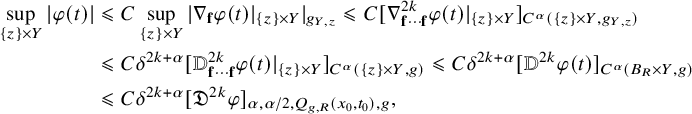 $$ \begin{align}\begin{aligned} \sup_{\{z\}\times Y}|\varphi (t)|&\leqslant C\sup_{\{z\}\times Y}|\nabla_{\mathbf{f}}\varphi (t)|_{\{z\}\times Y}|_{g_{Y,z}}\leqslant C[\nabla^{2k}_{\mathbf{f\cdots f}}\varphi (t)|_{\{z\}\times Y}]_{C^{\alpha}(\{z\}\times Y, g_{Y,z})}\\ &\leqslant C\delta^{2k+\alpha}[{\mathbb{D}}^{2k}_{\mathbf{f\cdots f}}\varphi (t)|_{\{z\}\times Y}]_{C^{\alpha}(\{z\}\times Y,g)} \leqslant C\delta^{2k+\alpha}[{\mathbb{D}}^{2k}\varphi (t)]_{C^{\alpha}(B_R\times Y,g)}\\ &\leqslant C\delta^{2k+\alpha}[\mathfrak{D}^{2k}\varphi ]_{{\alpha},{\alpha}/2,Q_{g,R}(x_0,t_0),g}, \end{aligned}\end{align} $$
where in the second inequality, we used [Reference Hein and Tosatti21, Lemma 2.10], and (2.37) follows when
 $k\geqslant 1$
. Lastly, when
$k\geqslant 1$
. Lastly, when
 $k=0$
, the argument is straightforward: using again that
$k=0$
, the argument is straightforward: using again that
 $\underline{\varphi }(t)=0$
, we bound
$\underline{\varphi }(t)=0$
, we bound
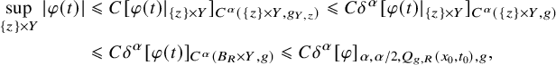 $$ \begin{align} \begin{aligned} \sup_{\{z\}\times Y}|\varphi (t)|&\leqslant C[\varphi (t)|_{\{z\}\times Y}]_{C^{\alpha}(\{z\}\times Y, g_{Y,z})}\leqslant C\delta^{\alpha}[\varphi (t)|_{\{z\}\times Y}]_{C^{\alpha}(\{z\}\times Y,g)}\\ &\leqslant C\delta^{\alpha}[\varphi (t)]_{C^{\alpha}(B_R\times Y,g)}\leqslant C\delta^{\alpha}[\varphi ]_{{\alpha},{\alpha}/2,Q_{g,R}(x_0,t_0),g}, \end{aligned}\end{align} $$
which completes the proof of (2.34) and (2.35) for
 $\varphi $
. Lastly, the analogous estimates for
$\varphi $
. Lastly, the analogous estimates for
 $\eta ={i\partial \bar \partial }\varphi $
follow in a similar fashion, by first using interpolation Proposition 2.3 to reduce ourselves to proving
$\eta ={i\partial \bar \partial }\varphi $
follow in a similar fashion, by first using interpolation Proposition 2.3 to reduce ourselves to proving
 $$ \begin{align} \|\eta\|_{\infty,Q_{g,\rho}(x_0,t_0),g}\leqslant C \delta^{2k+{\alpha}}[ \mathfrak{D}^{2k} \eta]_{{\alpha},{\alpha}/2,Q_{g,R}(x_0,t_0),g}, \end{align} $$
and then proving (2.40) by freezing the time variable t and applying [Reference Hein and Tosatti21, (2.61)] to
 $\eta (\cdot , t)$
and getting
$\eta (\cdot , t)$
and getting
 $$ \begin{align} \|\eta(t)\|_{\infty,B_R\times Y,g}\leqslant C \delta^{2k+{\alpha}}[ {\mathbb{D}}^{2k} \eta]_{C^{\alpha}(B_R\times Y,g)}\leqslant C \delta^{2k+{\alpha}}[ \mathfrak{D}^{2k} \eta]_{{\alpha},{\alpha}/2,Q_{g,R}(x_0,t_0),g}, \end{align} $$
which concludes the proof.
2.6 Parabolic Schauder estimates
In the course of the proof of our main Theorem, we also need two parabolic Schauder estimates on cylinders, which will be used when linearizing the Kähler-Ricci flow equation, and which are analogs of [Reference Hein and Tosatti21, Proposition 2.15]. Let
 $(z_{\ell },y_{\ell })\to (z_\infty ,y_\infty )$
be a convergent family of points in
$(z_{\ell },y_{\ell })\to (z_\infty ,y_\infty )$
be a convergent family of points in
 $B\times Y$
. For
$B\times Y$
. For
 $\ell \geqslant 1$
, consider the diffeomorphism
$\ell \geqslant 1$
, consider the diffeomorphism
 $\Lambda _{\ell }: (\check z,\check y)\mapsto (z_{\ell }+e^{-t_{\ell }/2}\check z,\check y)$
, and let
$\Lambda _{\ell }: (\check z,\check y)\mapsto (z_{\ell }+e^{-t_{\ell }/2}\check z,\check y)$
, and let
 $\check J_{\ell }$
be the pullback of the complex structure J via
$\check J_{\ell }$
be the pullback of the complex structure J via
 $\Lambda _{\ell }$
, which converges to
$\Lambda _{\ell }$
, which converges to
 $\check J_\infty =J_{\mathbb {C}^m}+J_{Y,z_\infty }$
locally smoothly. Similarly, we let
$\check J_\infty =J_{\mathbb {C}^m}+J_{Y,z_\infty }$
locally smoothly. Similarly, we let
 $\check {{\mathbb {D}}}_{\ell }$
denote the pullback of the connection
$\check {{\mathbb {D}}}_{\ell }$
denote the pullback of the connection
 ${\mathbb {D}}$
so that
${\mathbb {D}}$
so that
 $\check {{\mathbb {D}}}_{\ell }\to \check {{\mathbb {D}}}_\infty =\nabla ^{\mathbb {C}^m}+\nabla ^{g_{Y,z_\infty }}$
locally smoothly in spacetime. By the translation, we may assume that our new base point is
$\check {{\mathbb {D}}}_{\ell }\to \check {{\mathbb {D}}}_\infty =\nabla ^{\mathbb {C}^m}+\nabla ^{g_{Y,z_\infty }}$
locally smoothly in spacetime. By the translation, we may assume that our new base point is
 $\check p_{\ell }=(\check z_{\ell },\check y_{\ell })=(0,\check y_{\ell })\to (0,\check y_\infty )$
. We rescale the geometric quantities in a parabolic way centered at
$\check p_{\ell }=(\check z_{\ell },\check y_{\ell })=(0,\check y_{\ell })\to (0,\check y_\infty )$
. We rescale the geometric quantities in a parabolic way centered at
 $t_{\ell }$
, such as, for example,
$t_{\ell }$
, such as, for example,
 $\check g_{\ell }(\check t)=e^{t_{\ell }}\Lambda _{\ell }^{*} g(t_{\ell }+e^{-t_{\ell }}\check t),$
where recall that we denote by
$\check g_{\ell }(\check t)=e^{t_{\ell }}\Lambda _{\ell }^{*} g(t_{\ell }+e^{-t_{\ell }}\check t),$
where recall that we denote by
 $g(t)=g_{\mathbb {C}^m}+e^{-t}g_{Y,0}$
, so that
$g(t)=g_{\mathbb {C}^m}+e^{-t}g_{Y,0}$
, so that
 $\check {g}_{\ell }(0)=g_{\mathbb {C}^m}+g_{Y,0}$
.
$\check {g}_{\ell }(0)=g_{\mathbb {C}^m}+g_{Y,0}$
.
The first Schauder estimate is for scalar functions:
Proposition 2.8. Let
 $U\subset \mathbb {C}^m\times Y$
be an open set containing
$U\subset \mathbb {C}^m\times Y$
be an open set containing
 $(0,y_\infty )$
. Let
$(0,y_\infty )$
. Let
 $\check g_{\ell }, \check {\omega }_{\ell }^\sharp $
be Riemannian resp.
$\check g_{\ell }, \check {\omega }_{\ell }^\sharp $
be Riemannian resp.
 $\check J_{\ell }$
-Kähler metrics on U that converge locally smoothly to a Riemannian resp.
$\check J_{\ell }$
-Kähler metrics on U that converge locally smoothly to a Riemannian resp.
 $\check J_\infty $
-Kähler metric
$\check J_\infty $
-Kähler metric
 $\check {g}_\infty ,\check {\omega }_\infty ^\sharp $
on U. Then for all
$\check {g}_\infty ,\check {\omega }_\infty ^\sharp $
on U. Then for all
 $a\in \mathbb {N}_{>0}$
,
$a\in \mathbb {N}_{>0}$
,
 ${\alpha }\in (0,1)$
and
${\alpha }\in (0,1)$
and
 $R>0$
, there exists
$R>0$
, there exists
 $\ell _0>0$
and
$\ell _0>0$
and
 $C>0$
such that for all
$C>0$
such that for all
 $0<\rho <R$
,
$0<\rho <R$
,
 $\ell \geqslant \ell _0$
and all smooth function u defined on
$\ell \geqslant \ell _0$
and all smooth function u defined on
 $U\times \mathbb {R}$
, we have that
$U\times \mathbb {R}$
, we have that
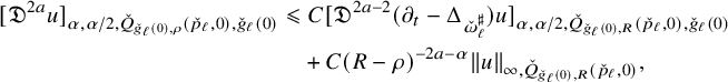 $$ \begin{align} \begin{aligned} [\mathfrak{D}^{2a} u]_{{\alpha},{\alpha}/2,\check Q_{\check g_{\ell}(0),\rho}(\check p_{\ell},0 ),\check g_{\ell}(0)}&\leqslant C[ \mathfrak{D}^{2a-2}(\partial_t-\Delta_{\check \omega_{\ell}^\sharp})u]_{{\alpha},{\alpha}/2,\check Q_{\check g_{\ell}(0),R}(\check p_{\ell},0 ),\check g_{\ell}(0)}\\&\quad +C(R-\rho)^{-2a-{\alpha}} \|u\|_{\infty,\check Q_{\check g_{\ell}(0),R}(\check p_{\ell},0 )}, \end{aligned} \end{align} $$
whenever
 $\check Q_{\check g_{\ell }(0),R}(\check p_{\ell },0 )\subset U\times \mathbb {R}$
.
$\check Q_{\check g_{\ell }(0),R}(\check p_{\ell },0 )\subset U\times \mathbb {R}$
.
Proof. We let
 $\sigma $
be small enough so that with respect to
$\sigma $
be small enough so that with respect to
 $\check g_\infty =g_{\mathbb {C}^m}+g_{Y,z_\infty }$
, the
$\check g_\infty =g_{\mathbb {C}^m}+g_{Y,z_\infty }$
, the
 $\check g_\infty $
-geodesic ball of size
$\check g_\infty $
-geodesic ball of size
 $\sigma $
is geodesically convex and admits a normal coordinate chart centered at any
$\sigma $
is geodesically convex and admits a normal coordinate chart centered at any
 $(z,y)\in \mathbb {C}^m\times Y$
. This is possible since Y is compact and
$(z,y)\in \mathbb {C}^m\times Y$
. This is possible since Y is compact and
 $\mathbb {C}^m$
is flat with respect to
$\mathbb {C}^m$
is flat with respect to
 $\check g_\infty $
. Since
$\check g_\infty $
. Since
 $\check g_{\ell }(t)\to g_{\mathbb {C}^m}+g_{Y,z_\infty }$
as
$\check g_{\ell }(t)\to g_{\mathbb {C}^m}+g_{Y,z_\infty }$
as
 $\ell \to +\infty $
and
$\ell \to +\infty $
and
 $\check {\mathbb {D}}_{\ell }\to \check {\mathbb {D}}_\infty $
locally smoothly, for any large
$\check {\mathbb {D}}_{\ell }\to \check {\mathbb {D}}_\infty $
locally smoothly, for any large
 $R>0$
, there exists
$R>0$
, there exists
 $\ell _0$
such that for all
$\ell _0$
such that for all
 $\ell>\ell _0$
and
$\ell>\ell _0$
and
 $(\check p,\check t)\in \check Q_{\check g_{\ell }(0),2R}(\check p_{\ell },0)$
,
$(\check p,\check t)\in \check Q_{\check g_{\ell }(0),2R}(\check p_{\ell },0)$
,
 $B_{\check g_{\ell }(0)}(\check p,\sigma )$
is geodesically convex and is compactly contained in a Euclidean ball of radius
$B_{\check g_{\ell }(0)}(\check p,\sigma )$
is geodesically convex and is compactly contained in a Euclidean ball of radius
 $2\sigma $
. Moreover, we can assume that the Kähler structure
$2\sigma $
. Moreover, we can assume that the Kähler structure
 $\check {\omega }^\sharp _{\ell }, \check J_{\ell }$
is smoothly close to the product structure
$\check {\omega }^\sharp _{\ell }, \check J_{\ell }$
is smoothly close to the product structure
 $\check {\omega }^\sharp _\infty , \check {J}_\infty $
in the parabolic domain
$\check {\omega }^\sharp _\infty , \check {J}_\infty $
in the parabolic domain
 $\check Q_{\check g_{\ell }(0),2R}(\check p_{\ell },0 )$
.
$\check Q_{\check g_{\ell }(0),2R}(\check p_{\ell },0 )$
.
The product metric
 $\check g_{\ell }(0)$
is uniformly comparable to the Euclidean metric on
$\check g_{\ell }(0)$
is uniformly comparable to the Euclidean metric on
 $\check Q_{\check g_{\ell }(0),\sigma }(\check p,\check t)$
for all
$\check Q_{\check g_{\ell }(0),\sigma }(\check p,\check t)$
for all
 $(\check p,\check t)\in \check Q_{\check g_{\ell }(0),R}(\check p_{\ell },0 )$
. By the standard Euclidean parabolic Schauder estimates (see, for example, [Reference Lieberman29, Theorem 4.9 and p.84]), there exists
$(\check p,\check t)\in \check Q_{\check g_{\ell }(0),R}(\check p_{\ell },0 )$
. By the standard Euclidean parabolic Schauder estimates (see, for example, [Reference Lieberman29, Theorem 4.9 and p.84]), there exists
 $C>0$
such that for all
$C>0$
such that for all
 $0<\rho _1<\rho _2<\sigma $
, and functions u on
$0<\rho _1<\rho _2<\sigma $
, and functions u on
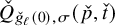 $\check Q_{\check g_{\ell }(0),\sigma }(\check p,\check t)$
where
$\check Q_{\check g_{\ell }(0),\sigma }(\check p,\check t)$
where
 $(\check p,\check t)\in \check Q_{\check g_{\ell }(0),R}(\check p_{\ell },0 )$
, we have
$(\check p,\check t)\in \check Q_{\check g_{\ell }(0),R}(\check p_{\ell },0 )$
, we have
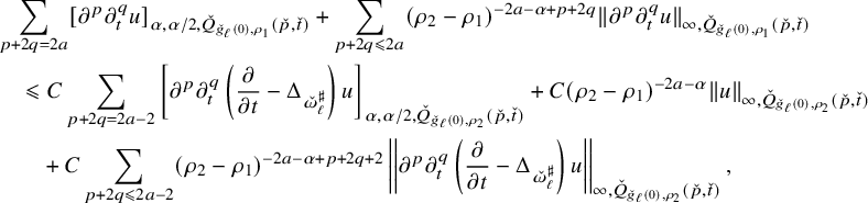 $$ \begin{align} \begin{aligned} &\sum_{p+2q=2a}[\partial^{p}\partial_t^qu]_{{\alpha},{\alpha}/2,\check Q_{\check g_{\ell}(0),\rho_1}(\check p,\check t)}+ \sum_{p+2q\leqslant 2a}(\rho_2-\rho_1)^{-2a-{\alpha}+p+2q}\|\partial^{p}\partial_t^qu\|_{\infty,\check Q_{\check g_{\ell}(0),\rho_1}(\check p,\check t)} \\&\quad\leqslant C \sum_{p+2q=2a-2}\left[\partial^{p}\partial_t^q \left(\frac{\partial}{\partial t}-\Delta_{\check\omega_{\ell}^\sharp}\right)u\right]_{{\alpha},{\alpha}/2,\check Q_{\check g_{\ell}(0),\rho_2}(\check p,\check t)} + C(\rho_2-\rho_1)^{-2a-{\alpha}}\| u\|_{\infty,\check Q_{\check g_{\ell}(0),\rho_2}(\check p,\check t)}\\&\qquad +C\sum_{p+2q\leqslant 2a-2}(\rho_2-\rho_1)^{-2a-{\alpha}+p+2q+2}\left|\left|\partial^{p}\partial_t^q \left(\frac{\partial}{\partial t}-\Delta_{\check\omega_{\ell}^\sharp}\right)u\right|\right|_{\infty,\check Q_{\check g_{\ell}(0),\rho_2}(\check p,\check t)}, \end{aligned} \end{align} $$
where the derivatives, Hölder norms are computed using the standard Euclidean metric and
 $\Delta _{\check \omega _{\ell }^\sharp }$
denotes the Laplacian of the metric
$\Delta _{\check \omega _{\ell }^\sharp }$
denotes the Laplacian of the metric
 $\check \omega _{\ell }^\sharp $
.
$\check \omega _{\ell }^\sharp $
.
We first use interpolation to eliminate the terms in the last line of (2.43). For
 $0<\rho _1<\rho _2<\sigma $
, we let
$0<\rho _1<\rho _2<\sigma $
, we let
 $\rho _2^{\prime }=\frac 12 (\rho _1+\rho _2)$
so that (2.43) holds with
$\rho _2^{\prime }=\frac 12 (\rho _1+\rho _2)$
so that (2.43) holds with
 $\rho _2$
replaced by
$\rho _2$
replaced by
 $\rho _2^{\prime }$
and C replaced by a slightly larger C. Hence, the standard Euclidean interpolation (or Proposition 2.3) yields
$\rho _2^{\prime }$
and C replaced by a slightly larger C. Hence, the standard Euclidean interpolation (or Proposition 2.3) yields
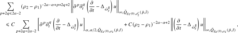 $$ \begin{align} \begin{aligned} &\sum_{p+2q\leqslant 2a-2}(\rho_2-\rho_1)^{-2a-{\alpha}+p+2q+2}\left|\left|\partial^{p}\partial_t^q \left(\frac{\partial}{\partial t}-\Delta_{\check\omega_{\ell}^\sharp}\right)u\right|\right|_{\infty,\check Q_{\check g_{\ell}(0),\rho_2^{\prime}}(\check p,\check t)}\\&\quad\leqslant C \sum_{p+2q=2a-2}\left[\partial^{p}\partial_t^q \left(\frac{\partial}{\partial t}-\Delta_{\check\omega_{\ell}^\sharp}\right)u\right]_{{\alpha},{\alpha}/2,\check Q_{\check g_{\ell}(0),\rho_2}(\check p,\check t)} + C(\rho_2-\rho_1)^{-2a-{\alpha}+2}\left|\left| \left(\frac{\partial}{\partial t}-\Delta_{\check\omega_{\ell}^\sharp}\right)u\right|\right|_{\infty,\check Q_{\check g_{\ell}(0),\rho_2}(\check p,\check t)}, \end{aligned} \end{align} $$
where we have used
 $\rho _2^{\prime }-\rho _2=\frac 12 (\rho _2-\rho _1)$
.
$\rho _2^{\prime }-\rho _2=\frac 12 (\rho _2-\rho _1)$
.
We now want to estimate the
 $L^\infty $
norm of
$L^\infty $
norm of
 $\left(\frac {\partial }{\partial t}-\Delta _{\check \omega _{\ell }^\sharp }\right)u$
in terms of the
$\left(\frac {\partial }{\partial t}-\Delta _{\check \omega _{\ell }^\sharp }\right)u$
in terms of the
 $L^\infty $
norm of u and of the Hölder seminorm of top order derivatives of u. To do this, we interpolate again. Let
$L^\infty $
norm of u and of the Hölder seminorm of top order derivatives of u. To do this, we interpolate again. Let
 $\varepsilon \in (0,1)$
be a small constant to be determined, and given
$\varepsilon \in (0,1)$
be a small constant to be determined, and given
 $0<\rho _1<\rho _2<\sigma $
, denote
$0<\rho _1<\rho _2<\sigma $
, denote
 $\rho _2^{\prime \prime }=\rho _1+(1-\varepsilon ) (\rho _2-\rho _1)$
. We consider (2.44) with
$\rho _2^{\prime \prime }=\rho _1+(1-\varepsilon ) (\rho _2-\rho _1)$
. We consider (2.44) with
 $\rho _2$
replaced by
$\rho _2$
replaced by
 $\rho _2^{\prime \prime }$
. Since
$\rho _2^{\prime \prime }$
. Since
 $\check \omega _{\ell }^\sharp $
is uniformly bounded in
$\check \omega _{\ell }^\sharp $
is uniformly bounded in
 $C^\infty $
, the standard Euclidean interpolation (or Proposition 2.3) yields
$C^\infty $
, the standard Euclidean interpolation (or Proposition 2.3) yields
 $$ \begin{align} \begin{aligned} &(\rho_2^{\prime\prime}-\rho_1)^{-2a-{\alpha}+2}\left|\left| \left(\frac{\partial}{\partial t}-\Delta_{\check\omega_{\ell}^\sharp}\right)u\right|\right|_{\infty,\check Q_{\check g_{\ell}(0),\rho_2^{\prime\prime}}(\check p,\check t)}\\&\quad=\left(\frac{\varepsilon}{1-\varepsilon} \right)^{2a+{\alpha}-2}(\rho_2-\rho_2^{\prime\prime})^{-2a-{\alpha}+2}\left|\left| \left(\frac{\partial}{\partial t}-\Delta_{\check\omega_{\ell}^\sharp}\right)u\right|\right|_{\infty,\check Q_{\check g_{\ell}(0),\rho_2^{\prime\prime}}(\check p,\check t)}\\&\quad\leqslant C\left(\frac{\varepsilon}{1-\varepsilon} \right)^{2a+{\alpha}-2}\left(\sum_{p+2q=2a}\left[\partial^p\partial_t^q u \right]_{{\alpha},{\alpha}/2,\check Q_{\check g_{\ell}(0),\rho_2}(\check p,\check t)}+(\rho_2-\rho_2^{\prime\prime})^{-2a-{\alpha}} \|u\|_{\infty,\check Q_{\check g_{\ell}(0),\rho_2}(\check p,\check t)}\right). \end{aligned} \end{align} $$
Therefore, inserting (2.44) and (2.45) into (2.43), we can choose
 $\varepsilon $
sufficiently small so that
$\varepsilon $
sufficiently small so that
 $$ \begin{align} \begin{aligned} &\sum_{p+2q=2a}[\partial^{p}\partial_t^qu]_{{\alpha},{\alpha}/2,\check Q_{\check g_{\ell}(0),\rho_1}(\check p,\check t)}+ \sum_{p+2q\leqslant 2a}(\rho_2-\rho_1)^{-2a-{\alpha}+p+2q}\|\partial^{p}\partial_t^qu\|_{\infty,\check Q_{\check g_{\ell}(0),\rho_1}(\check p,\check t)} \\&\quad\leqslant C \sum_{p+2q=2a-2}\left[\partial^{p}\partial_t^q \left(\frac{\partial}{\partial t}-\Delta_{\check\omega_{\ell}^\sharp}\right)u\right]_{{\alpha},{\alpha}/2,\check Q_{\check g_{\ell}(0),\rho_2}(\check p,\check t)} + C(\rho_2-\rho_1)^{-2a-{\alpha}}\| u\|_{\infty,\check Q_{\check g_{\ell}(0),\rho_2}(\check p,\check t)}\\&\qquad +\frac12 \sum_{p+2q=2a}[\partial^{p}\partial_t^qu]_{{\alpha},{\alpha}/2,\check Q_{\check g_{\ell}(0),\rho_2}(\check p,\check t)}, \end{aligned} \end{align} $$
for all
 $0<\rho _1<\rho _2<\sigma $
. We can then apply the iteration lemma in [Reference Hein and Tosatti21, Lemma 2.9] to obtain
$0<\rho _1<\rho _2<\sigma $
. We can then apply the iteration lemma in [Reference Hein and Tosatti21, Lemma 2.9] to obtain
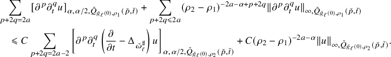 $$ \begin{align} \begin{aligned} &\sum_{p+2q=2a}[\partial^{p}\partial_t^qu]_{{\alpha},{\alpha}/2,\check Q_{\check g_{\ell}(0),\rho_1}(\check p,\check t)}+ \sum_{p+2q\leqslant 2a}(\rho_2-\rho_1)^{-2a-{\alpha}+p+2q}\|\partial^{p}\partial_t^qu\|_{\infty,\check Q_{\check g_{\ell}(0),\rho_1}(\check p,\check t)} \\&\quad\leqslant C \sum_{p+2q=2a-2}\left[\partial^{p}\partial_t^q \left(\frac{\partial}{\partial t}-\Delta_{\check\omega_{\ell}^\sharp}\right)u\right]_{{\alpha},{\alpha}/2,\check Q_{\check g_{\ell}(0),\rho_2}(\check p,\check t)} + C(\rho_2-\rho_1)^{-2a-{\alpha}}\| u\|_{\infty,\check Q_{\check g_{\ell}(0),\rho_2}(\check p,\check t)}. \end{aligned} \end{align} $$
We now claim that one can interchange the Euclidean derivatives
 $\partial $
and Euclidean parallel transport P in the definition of Hölder norms with
$\partial $
and Euclidean parallel transport P in the definition of Hölder norms with
 $\check {\mathbb {D}}_{\ell }$
and
$\check {\mathbb {D}}_{\ell }$
and
 $\check {\mathbb {P}}_{\ell }$
. Although in our definition of Hölder norms we only consider horizontal and vertical
$\check {\mathbb {P}}_{\ell }$
. Although in our definition of Hölder norms we only consider horizontal and vertical
 $\mathbb {P}$
-geodesics while the standard Euclidean Hölder norms consider all possible segments, it is immediate to see from [Reference Hein and Tosatti21, (2.31)] that the difference is harmless. To compare
$\mathbb {P}$
-geodesics while the standard Euclidean Hölder norms consider all possible segments, it is immediate to see from [Reference Hein and Tosatti21, (2.31)] that the difference is harmless. To compare
 $\partial $
with
$\partial $
with
 $\check {\mathbb {D}}_{\ell }$
, we note that on each
$\check {\mathbb {D}}_{\ell }$
, we note that on each
 $\check Q_{\check g_{\ell }(0),\sigma }(\check p,\check t)$
, we can write
$\check Q_{\check g_{\ell }(0),\sigma }(\check p,\check t)$
, we can write
 $\partial =\check {\mathbb {D}}_{\ell }+\check \Gamma _{\ell }$
(indeed independent of
$\partial =\check {\mathbb {D}}_{\ell }+\check \Gamma _{\ell }$
(indeed independent of
 $\check {t}$
) so that
$\check {t}$
) so that
 $\check \Gamma _{\ell }\to \check \Gamma _\infty $
where
$\check \Gamma _{\ell }\to \check \Gamma _\infty $
where
 $\check \Gamma _\infty (\check p)=0$
by our choice of normal coordinate centered at
$\check \Gamma _\infty (\check p)=0$
by our choice of normal coordinate centered at
 $\check p$
. In particular, the local smooth convergence implies that
$\check p$
. In particular, the local smooth convergence implies that
 $\check \Gamma _{\ell }\to 0$
in
$\check \Gamma _{\ell }\to 0$
in
 $C^k$
for fixed k uniformly as
$C^k$
for fixed k uniformly as
 $\ell \to +\infty $
and
$\ell \to +\infty $
and
 $\sigma \to 0$
, and then ODE estimates show that
$\sigma \to 0$
, and then ODE estimates show that
 $P-\check {\mathbb {P}}_{\ell }\to 0$
in
$P-\check {\mathbb {P}}_{\ell }\to 0$
in
 $C^k$
. In particular, switching from
$C^k$
. In particular, switching from
 $\partial ^p$
to
$\partial ^p$
to
 $\check {\mathbb {D}}_{\ell }^p$
will generate an error of the form (ignoring combinatorial constants):
$\check {\mathbb {D}}_{\ell }^p$
will generate an error of the form (ignoring combinatorial constants):
 $$ \begin{align} \left(\check {\mathbb{D}}_{\ell}^a-\partial^a\right) u=\sum_{i+j_1+\dots+j_q+q=a,q>0} \partial^{i}u \circledast \partial^{j_1}\check \Gamma_{\ell}\circledast \dots\circledast \partial^{j_q}\check \Gamma_{\ell}. \end{align} $$
Since
 $0<\rho _1<\rho _2\leqslant \sigma <1$
, and since all terms in (2.48) with
$0<\rho _1<\rho _2\leqslant \sigma <1$
, and since all terms in (2.48) with
 $\check {\Gamma }_{\ell }$
are
$\check {\Gamma }_{\ell }$
are
 $o(1)$
, the right-hand side in (2.48) can be absorbed in the second term in the left-hand side of (2.43). Thus, going back to (2.47), we can change the
$o(1)$
, the right-hand side in (2.48) can be absorbed in the second term in the left-hand side of (2.43). Thus, going back to (2.47), we can change the
 $\partial ,P$
with
$\partial ,P$
with
 $\check {D}_{\ell },\check {\mathbb {P}}_{\ell }$
, and using interpolation again, we obtain
$\check {D}_{\ell },\check {\mathbb {P}}_{\ell }$
, and using interpolation again, we obtain
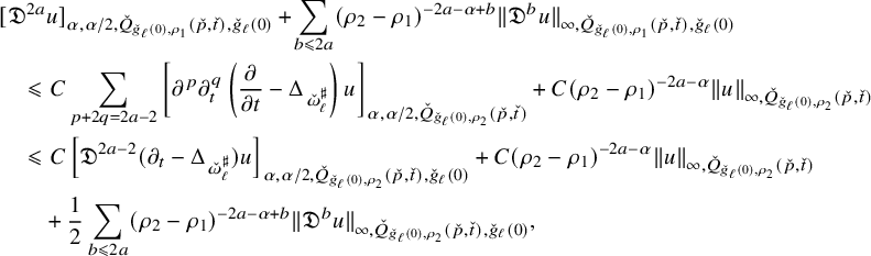 $$ \begin{align} \kern-10pt\begin{aligned} &[\mathfrak{D}^{2a} u]_{{\alpha},{\alpha}/2,\check Q_{\check g_{\ell}(0),\rho_1}(\check p,\check t),\check g_{\ell}(0)}+\! \sum_{b\leqslant 2a}(\rho_2-\rho_1)^{-2a-{\alpha}+b}\|\mathfrak{D}^bu\|_{\infty,\check Q_{\check g_{\ell}(0),\rho_1}(\check p,\check t),\check g_{\ell}(0)} \\&\quad\leqslant C \sum_{p+2q=2a-2}\left[\partial^{p}\partial_t^q \left(\frac{\partial}{\partial t}-\Delta_{\check \omega_{\ell}^\sharp}\right) u\right]_{{\alpha},{\alpha}/2,\check Q_{\check g_{\ell}(0),\rho_2}(\check p,\check t)} + C(\rho_2-\rho_1)^{-2a-{\alpha}}\| u\|_{\infty,\check Q_{\check g_{\ell}(0),\rho_2}(\check p,\check t)}\\&\quad\leqslant C \left[\mathfrak{D}^{2a-2} (\partial_t-\Delta_{\check \omega_{\ell}^\sharp}) u\right]_{{\alpha},{\alpha}/2,\check Q_{\check g_{\ell}(0),\rho_2}(\check p,\check t),\check g_{\ell}(0)} + C(\rho_2-\rho_1)^{-2a-{\alpha}}\| u\|_{\infty,\check Q_{\check g_{\ell}(0),\rho_2}(\check p,\check t)}\\&\qquad + \frac12 \sum_{b\leqslant 2a}(\rho_2-\rho_1)^{-2a-{\alpha}+b}\|\mathfrak{D}^bu\|_{\infty,\check Q_{\check g_{\ell}(0),\rho_2}(\check p,\check t),\check g_{\ell}(0)}, \end{aligned} \end{align} $$
where the coefficient
 $\frac 12$
in the last term is achieved by choosing
$\frac 12$
in the last term is achieved by choosing
 $\sigma $
sufficiently small thanks to the local smooth convergence of
$\sigma $
sufficiently small thanks to the local smooth convergence of
 $\check \Gamma _{\ell }$
. We fix
$\check \Gamma _{\ell }$
. We fix
 $\sigma $
from now on. It now follows from [Reference Hein and Tosatti21, Lemma 2.9] again that we have
$\sigma $
from now on. It now follows from [Reference Hein and Tosatti21, Lemma 2.9] again that we have
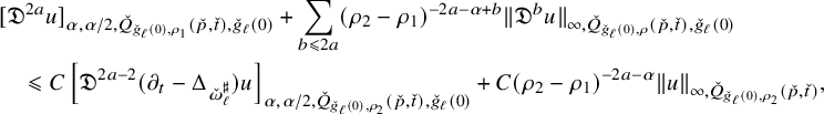 $$ \begin{align} \begin{aligned} &[\mathfrak{D}^{2a} u]_{{\alpha},{\alpha}/2,\check Q_{\check g_{\ell}(0),\rho_1}(\check p,\check t),\check g_{\ell}(0)}+ \sum_{b\leqslant 2a}(\rho_2-\rho_1)^{-2a-{\alpha}+b}\|\mathfrak{D}^bu\|_{\infty,\check Q_{\check g_{\ell}(0),\rho}(\check p,\check t),\check g_{\ell}(0)} \\&\quad\leqslant C \left[\mathfrak{D}^{2a-2} (\partial_t-\Delta_{\check \omega_{\ell}^\sharp}) u\right]_{{\alpha},{\alpha}/2,\check Q_{\check g_{\ell}(0),\rho_2}(\check p,\check t),\check g_{\ell}(0)} + C(\rho_2-\rho_1)^{-2a-{\alpha}}\| u\|_{\infty,\check Q_{\check g_{\ell}(0),\rho_2}(\check p,\check t)}, \end{aligned} \end{align} $$
for all
 $0<\rho _1<\rho _2<\sigma $
. This in particular shows the desired conclusion for all small
$0<\rho _1<\rho _2<\sigma $
. This in particular shows the desired conclusion for all small
 $0<\rho _1<\rho _2<\sigma $
with arbitrary center
$0<\rho _1<\rho _2<\sigma $
with arbitrary center
 $(\check p,\check t)$
in the compact set
$(\check p,\check t)$
in the compact set
 $ \check Q_{\check g_{\ell }(0),R}(\check p,0 )$
.
$ \check Q_{\check g_{\ell }(0),R}(\check p,0 )$
.
Now we prove the Hölder control on
 $ \check Q_{\check g_{\ell }(0),\rho }(\check p_{\ell },0 )$
for
$ \check Q_{\check g_{\ell }(0),\rho }(\check p_{\ell },0 )$
for
 $0<\rho <R$
. We can assume
$0<\rho <R$
. We can assume
 $R\geqslant \sigma $
. If
$R\geqslant \sigma $
. If
 $\rho <\frac 12 \sigma \leqslant \frac 12 R$
so that
$\rho <\frac 12 \sigma \leqslant \frac 12 R$
so that
 $\sigma -\rho \geqslant \frac 12\sigma \geqslant C^{-1}(R-\rho )$
, then (2.50) implies
$\sigma -\rho \geqslant \frac 12\sigma \geqslant C^{-1}(R-\rho )$
, then (2.50) implies
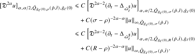
Hence, it remains to consider the case
 $\rho \geqslant \frac 12\sigma $
. Given any two points
$\rho \geqslant \frac 12\sigma $
. Given any two points
 $(\check p,\check t)$
and
$(\check p,\check t)$
and
 $(\check q,\check s)$
in
$(\check q,\check s)$
in
 $ \check Q_{\check g_{\ell }(0),\rho }(\check p_{\ell },0 )$
with
$ \check Q_{\check g_{\ell }(0),\rho }(\check p_{\ell },0 )$
with
 $r=d^{\check g_{\ell }(0)}(\check p,\check q)+|\check t-\check s|^{\frac {1}{2}}$
, we choose a sequence of points
$r=d^{\check g_{\ell }(0)}(\check p,\check q)+|\check t-\check s|^{\frac {1}{2}}$
, we choose a sequence of points
 $\{(\check p_i,\check t_i) \}_{i=1}^N$
inside
$\{(\check p_i,\check t_i) \}_{i=1}^N$
inside
 $\check Q_{\check g_{\ell }(0),\rho }(\check p_{\ell },0 )$
such that
$\check Q_{\check g_{\ell }(0),\rho }(\check p_{\ell },0 )$
such that
 $(\check p_1,\check t_1)=(\check p,\check t)$
and
$(\check p_1,\check t_1)=(\check p,\check t)$
and
 $(\check p_N,\check t_N)=(\check q,\check s)$
. We can choose them in a way so that
$(\check p_N,\check t_N)=(\check q,\check s)$
. We can choose them in a way so that
 $r_i=d^{\check g_{\ell }(0)}(\check p_i,\check p_{i+1})+|\check t_i-\check t_{i+1}|^{\frac {1}{2}}\leqslant \frac 14 \sigma $
is uniformly comparable to r and
$r_i=d^{\check g_{\ell }(0)}(\check p_i,\check p_{i+1})+|\check t_i-\check t_{i+1}|^{\frac {1}{2}}\leqslant \frac 14 \sigma $
is uniformly comparable to r and
 $N\leqslant C \sigma ^{-2}$
. Here, the square comes from the time direction. Moreover, we can assume
$N\leqslant C \sigma ^{-2}$
. Here, the square comes from the time direction. Moreover, we can assume
 $ \check Q_{\check g_{\ell }(0),\frac 14\sigma }(\check p_i,\check t_i)\subset \check Q_{\check g_{\ell }(0),\rho }(\check p_{\ell },0 ) $
for all
$ \check Q_{\check g_{\ell }(0),\frac 14\sigma }(\check p_i,\check t_i)\subset \check Q_{\check g_{\ell }(0),\rho }(\check p_{\ell },0 ) $
for all
 $i=2,\dots ,N-1$
(i.e., except
$i=2,\dots ,N-1$
(i.e., except
 $(\check p,\check t)$
and
$(\check p,\check t)$
and
 $(\check q,\check s)$
). For each
$(\check q,\check s)$
). For each
 $i=1,\dots ,N-1$
, we can apply (2.50) again to obtain
$i=1,\dots ,N-1$
, we can apply (2.50) again to obtain
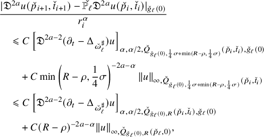 $$ \begin{align} \begin{aligned} &\frac{|\mathfrak{D}^{2a}u(\check p_{i+1},\check t_{i+1})- \check{\mathbb{P}_{\ell}}\mathfrak{D}^{2a}u(\check p_i,\check t_i)|_{\check g_{\ell}(0)}}{r_i^{\alpha}}\\&\quad\leqslant C \left[\mathfrak{D}^{2a-2} (\partial_t-\Delta_{\check \omega_{\ell}^\sharp}) u\right]_{{\alpha},{\alpha}/2,\check Q_{\check g_{\ell}(0),\frac14\sigma+\min(R-\rho,\frac14\sigma )}(\check p_i,\check t_i),\check g_{\ell}(0)}\\&\qquad + C\min\left(R-\rho,\frac14\sigma \right)^{-2a-{\alpha}}\| u\|_{\infty,\check Q_{\check g_{\ell}(0),\frac14\sigma+\min(R-\rho,\frac14\sigma )}(\check p_i,\check t_i)}\\&\quad\leqslant C \left[\mathfrak{D}^{2a-2} (\partial_t-\Delta_{\check \omega_{\ell}^\sharp}) u\right]_{{\alpha},{\alpha}/2,\check Q_{\check g_{\ell}(0),R}(\check p_i,\check t_i),\check g_{\ell}(0)}\\&\qquad + C(R-\rho)^{-2a-{\alpha}}\| u\|_{\infty,\check Q_{\check g_{\ell}(0),R}(\check p_{\ell},0)}, \end{aligned} \end{align} $$
for all
 $i=1,\dots ,N-1$
. Here, we have used the fact that
$i=1,\dots ,N-1$
. Here, we have used the fact that
 $\sigma \geqslant C^{-1}R\geqslant C^{-1}(R-\rho )$
. Since
$\sigma \geqslant C^{-1}R\geqslant C^{-1}(R-\rho )$
. Since
 $$ \begin{align} \frac{|\mathfrak{D}^{2a}u(\check p,\check t)- \check{\mathbb{P}_{\ell}}\mathfrak{D}^{2a}u(\check q,\check s)|_{\check g_{\ell}(0)}}{r^{\alpha}}\leqslant C\sum_{i=0}^{N-1} \frac{|\mathfrak{D}^{2a}u(\check p_{i+1},\check t_{i+1})- \check{\mathbb{P}_{\ell}}\mathfrak{D}^{2a}u(\check p_i,\check t_i)|_{\check g_{\ell}(0)}}{r_i^{\alpha}}, \end{align} $$
using (2.52) completes the proof after taking supremum over all
 $(\check p,\check t)$
and
$(\check p,\check t)$
and
 $(\check q,\check s)$
in
$(\check q,\check s)$
in
 $\check Q_{\check g_{\ell }(0),\rho }(\check p_{\ell },0 )$
.
$\check Q_{\check g_{\ell }(0),\rho }(\check p_{\ell },0 )$
.
The second Schauder estimate is for real
 $(1,1)$
-forms:
$(1,1)$
-forms:
Proposition 2.9. Let
 $U\subset \mathbb {C}^m\times Y$
be an open set containing
$U\subset \mathbb {C}^m\times Y$
be an open set containing
 $(0,y_\infty )$
. Let
$(0,y_\infty )$
. Let
 $\check g_{\ell }, \check {\omega }_{\ell }^\sharp $
be Riemannian resp.
$\check g_{\ell }, \check {\omega }_{\ell }^\sharp $
be Riemannian resp.
 $\check J_{\ell }$
-Kähler metrics on U that converges locally smoothly to a Riemannian resp.
$\check J_{\ell }$
-Kähler metrics on U that converges locally smoothly to a Riemannian resp.
 $\check J_\infty $
-Kähler metric
$\check J_\infty $
-Kähler metric
 $\check {g}_\infty ,\check {\omega }_\infty ^\sharp $
on U. Then for all
$\check {g}_\infty ,\check {\omega }_\infty ^\sharp $
on U. Then for all
 $a\in \mathbb {N}_{>0}$
,
$a\in \mathbb {N}_{>0}$
,
 ${\alpha }\in (0,1)$
and
${\alpha }\in (0,1)$
and
 $R>0$
, there exists
$R>0$
, there exists
 $\ell _0>0$
and
$\ell _0>0$
and
 $C>0$
such that for all
$C>0$
such that for all
 $0<\rho <R$
,
$0<\rho <R$
,
 $\ell \geqslant \ell _0$
and all real
$\ell \geqslant \ell _0$
and all real
 $\check {J}_{\ell }$
-
$\check {J}_{\ell }$
-
 $(1,1)$
form
$(1,1)$
form
 $\eta $
defined on
$\eta $
defined on
 $U\times \mathbb {R}$
, we have that
$U\times \mathbb {R}$
, we have that

whenever
 $\check Q_{\check g_{\ell }(0),R}(\check p_{\ell },0 )\subset U\times \mathbb {R}$
, and where
$\check Q_{\check g_{\ell }(0),R}(\check p_{\ell },0 )\subset U\times \mathbb {R}$
, and where
 $\Delta _{\check \omega _{\ell }^\sharp }\eta $
denotes the Hodge Laplacian of
$\Delta _{\check \omega _{\ell }^\sharp }\eta $
denotes the Hodge Laplacian of
 $\check \omega _{\ell }^\sharp $
acting on differential forms.
$\check \omega _{\ell }^\sharp $
acting on differential forms.
Proof. The proof shares some similarities with the proof of Proposition 2.8. After the same preliminary remarks as there, we first work in the Euclidean setting, with the Hodge Laplacian
 $\Delta _{\check \omega _{\ell }^\sharp }\eta $
. We can then apply standard parabolic Schauder estimate to the uniformly parabolic system given by
$\Delta _{\check \omega _{\ell }^\sharp }\eta $
. We can then apply standard parabolic Schauder estimate to the uniformly parabolic system given by
 $(\partial _t-\Delta _{\check \omega _{\ell }^\sharp })$
acting on real
$(\partial _t-\Delta _{\check \omega _{\ell }^\sharp })$
acting on real
 $(1,1)$
-forms [Reference Ladyženskaja, Solonnikov and Ural’ceva24, Chapter 7], which shows that there exists
$(1,1)$
-forms [Reference Ladyženskaja, Solonnikov and Ural’ceva24, Chapter 7], which shows that there exists
 $C>0$
such that for all
$C>0$
such that for all
 $0<\rho _1<\rho _2<\sigma $
, and
$0<\rho _1<\rho _2<\sigma $
, and
 $\eta $
lives in
$\eta $
lives in
 $\check Q_{\check g_{\ell }(0),\sigma }(\check p,\check t)$
where
$\check Q_{\check g_{\ell }(0),\sigma }(\check p,\check t)$
where
 $(\check p,\check t)\in \check Q_{\check g_{\ell }(0),R}(\check p_{\ell },0 )$
, we have
$(\check p,\check t)\in \check Q_{\check g_{\ell }(0),R}(\check p_{\ell },0 )$
, we have
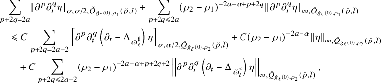 $$ \begin{align} \kern-15pt\begin{aligned} &\sum_{p+2q=2a}[\partial^{p}\partial_t^q\eta]_{{\alpha},{\alpha}/2,\check Q_{\check g_{\ell}(0),\rho_1}(\check p,\check t)}+ \sum_{p+2q\leqslant 2a}(\rho_2-\rho_1)^{-2a-{\alpha}+p+2q}\|\partial^{p}\partial_t^q \eta\|_{\infty,\check Q_{\check g_{\ell}(0),\rho_1}(\check p,\check t)} \\&\quad\leqslant C \sum_{p+2q=2a-2}\left[\partial^{p}\partial_t^q \left(\partial_t-\Delta_{\check\omega_{\ell}^\sharp} \right) \eta\right]_{{\alpha},{\alpha}/2,\check Q_{\check g_{\ell}(0),\rho_2}(\check p,\check t)} + C(\rho_2-\rho_1)^{-2a-{\alpha}}\| \eta\|_{\infty,\check Q_{\check g_{\ell}(0),\rho_2}(\check p,\check t)}\\&\qquad +C\sum_{p+2q\leqslant 2a-2}(\rho_2-\rho_1)^{-2a-{\alpha}+p+2q+2}\left|\left|\partial^{p}\partial_t^q\left(\partial_t-\Delta_{\check\omega_{\ell}^\sharp} \right) \eta\right|\right|_{\infty,\check Q_{\check g_{\ell}(0),\rho_2}(\check p,\check t)}, \end{aligned} \end{align} $$
where the derivatives and Hölder norms are computed using standard Euclidean metric.
We first eliminate the terms in the last line of (2.55) by interpolation: given
 $0<\rho _1<\rho _2<\sigma $
, we let
$0<\rho _1<\rho _2<\sigma $
, we let
 $\rho _2^{\prime }=\frac {1}{2}(\rho _1+\rho _2)$
, so that (2.55) holds with
$\rho _2^{\prime }=\frac {1}{2}(\rho _1+\rho _2)$
, so that (2.55) holds with
 $\rho _2$
replaced by
$\rho _2$
replaced by
 $\rho _2^{\prime }$
, and so standard interpolation gives
$\rho _2^{\prime }$
, and so standard interpolation gives
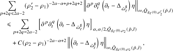 $$ \begin{align} \begin{aligned} &\sum_{p+2q\leqslant 2a-2}(\rho_2^{\prime}-\rho_1)^{-2a-{\alpha}+p+2q+2}\left|\left|\partial^{p}\partial_t^q\left(\partial_t-\Delta_{\check\omega_{\ell}^\sharp} \right) \eta\right|\right|_{\infty,\check Q_{\check g_{\ell}(0),\rho_2^{\prime}}(\check p,\check t)} \\&\quad\leqslant \sum_{p+2q= 2a-2}\left[\partial^{p}\partial_t^q\left(\partial_t-\Delta_{\check\omega_{\ell}^\sharp} \right) \eta\right]_{\alpha,\alpha/2,\check Q_{\check g_{\ell}(0),\rho_2}(\check p,\check t)}\\&\qquad +C(\rho_2-\rho_1)^{-2a-{\alpha}+2}\left\|\left(\partial_t-\Delta_{\check\omega_{\ell}^\sharp} \right) \eta\right\|_{\infty,\check Q_{\check g_{\ell}(0),\rho_2}(\check p,\check t)}, \end{aligned} \end{align} $$
using that
 $\rho ^{\prime }_2-\rho _2=\frac {1}{2}(\rho _2-\rho _1)$
. We now want to estimate the
$\rho ^{\prime }_2-\rho _2=\frac {1}{2}(\rho _2-\rho _1)$
. We now want to estimate the
 $L^\infty $
norm of
$L^\infty $
norm of
 $\left(\partial _t-\Delta _{\check \omega _{\ell }^\sharp } \right) \eta $
. Let
$\left(\partial _t-\Delta _{\check \omega _{\ell }^\sharp } \right) \eta $
. Let
 $\varepsilon \in (0,1)$
be a constant to be determined, and denote by
$\varepsilon \in (0,1)$
be a constant to be determined, and denote by
 $\rho _2^{\prime \prime }=\rho _2+\varepsilon (\rho _2-\rho _1)$
. By interpolation and the
$\rho _2^{\prime \prime }=\rho _2+\varepsilon (\rho _2-\rho _1)$
. By interpolation and the
 $C^\infty $
boundedness of
$C^\infty $
boundedness of
 $\check g_{\ell }^\sharp $
, we have
$\check g_{\ell }^\sharp $
, we have
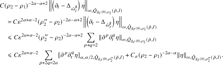 $$ \begin{align} \begin{aligned} &C(\rho_2-\rho_1)^{-2a-{\alpha}+2}\left|\left|\left(\partial_t-\Delta_{\check\omega_{\ell}^\sharp} \right) \eta\right|\right|_{\infty,\check Q_{\check g_{\ell}(0),\rho_2}(\check p,\check t)}\\&\quad=C\varepsilon^{2a+{\alpha}-2}(\rho_2^{\prime\prime}-\rho_2)^{-2a-{\alpha}+2}\left|\left|\left(\partial_t-\Delta_{\check\omega_{\ell}^\sharp} \right) \eta\right|\right|_{\infty,\check Q_{\check g_{\ell}(0),\rho_2}(\check p,\check t)}\\&\quad\leqslant C\varepsilon^{2a+{\alpha}-2}(\rho_2^{\prime\prime}-\rho_2)^{-2a-{\alpha}+2}\sum_{p+q=2}\|\partial^{p}\partial_t^q\eta\|_{\infty,\check Q_{\check g_{\ell}(0),\rho_2}(\check p,\check t)}\\&\quad\leqslant C\varepsilon^{2a+{\alpha}-2} \sum_{p+2q=2a}[\partial^{p}\partial_t^q\eta]_{{\alpha},{\alpha}/2,\check Q_{\check g_{\ell}(0),\rho_2^{\prime\prime}}(\check p,\check t)}+ C_\varepsilon(\rho_2-\rho_1)^{-2a-{\alpha}}\| \eta\|_{\infty,\check Q_{\check g_{\ell}(0),\rho_2^{\prime\prime}}(\check p,\check t)}. \end{aligned} \end{align} $$
Since
 $a\geqslant 1$
, we can choose
$a\geqslant 1$
, we can choose
 $\varepsilon $
small enough so that
$\varepsilon $
small enough so that
 $C\varepsilon ^{2a+{\alpha }-2}\leqslant \frac 12$
. Inserting this in (2.56) (replacing
$C\varepsilon ^{2a+{\alpha }-2}\leqslant \frac 12$
. Inserting this in (2.56) (replacing
 $\rho _2^{\prime \prime }$
by
$\rho _2^{\prime \prime }$
by
 $\rho _2$
), and plugging into (2.55) gives
$\rho _2$
), and plugging into (2.55) gives
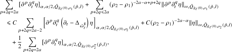 $$ \begin{align} \begin{aligned} &\sum_{p+2q=2a}[\partial^{p}\partial_t^q\eta]_{{\alpha},{\alpha}/2,\check Q_{\check g_{\ell}(0),\rho_1}(\check p,\check t)}+ \sum_{p+2q\leqslant 2a}(\rho_2-\rho_1)^{-2a-{\alpha}+p+2q}\|\partial^{p}\partial_t^q\eta\|_{\infty,\check Q_{\check g_{\ell}(0),\rho_1}(\check p,\check t)} \\&\quad\leqslant C \sum_{p+2q=2a-2}\left[\partial^{p}\partial_t^q \left(\partial_t-\Delta_{\check\omega_{\ell}^\sharp} \right) \eta\right]_{{\alpha},{\alpha}/2,\check Q_{\check g_{\ell}(0),\rho_2}(\check p,\check t)} + C(\rho_2-\rho_1)^{-2a-{\alpha}}\| \eta\|_{\infty,\check Q_{\check g_{\ell}(0),\rho_2}(\check p,\check t)}\\&\qquad +\frac{1}{2}\sum_{p+2q=2a}[\partial^{p}\partial_t^q\eta]_{{\alpha},{\alpha}/2,\check Q_{\check g_{\ell}(0),\rho_2^{\prime\prime}}(\check p,\check t)}, \end{aligned} \end{align} $$
and the iteration lemma in [Reference Hein and Tosatti21, Lemma 2.9] then gives
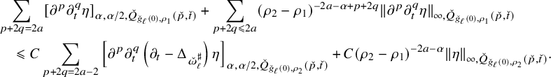 $$ \begin{align} \begin{aligned} &\sum_{p+2q=2a}[\partial^{p}\partial_t^q\eta]_{{\alpha},{\alpha}/2,\check Q_{\check g_{\ell}(0),\rho_1}(\check p,\check t)}+ \sum_{p+2q\leqslant 2a}(\rho_2-\rho_1)^{-2a-{\alpha}+p+2q}\|\partial^{p}\partial_t^q\eta\|_{\infty,\check Q_{\check g_{\ell}(0),\rho_1}(\check p,\check t)} \\&\quad\leqslant C \sum_{p+2q=2a-2}\left[\partial^{p}\partial_t^q \left(\partial_t-\Delta_{\check\omega_{\ell}^\sharp} \right) \eta\right]_{{\alpha},{\alpha}/2,\check Q_{\check g_{\ell}(0),\rho_2}(\check p,\check t)} + C(\rho_2-\rho_1)^{-2a-{\alpha}}\| \eta\|_{\infty,\check Q_{\check g_{\ell}(0),\rho_2}(\check p,\check t)}. \end{aligned} \end{align} $$
This is the direct analog of (2.47). After this, the rest of the proof of (2.54) proceeds exactly as in the proof of Proposition 2.8.
3 The Selection Theorem
In our main theorem, we will need the analog of the Selection Theorem [Reference Hein and Tosatti21, Theorem 3.11], adapted to our parabolic setting, and to the specific structure of the parabolic complex Monge-Ampère equation that we are dealing with. As in [Reference Hein and Tosatti21], to state this, we will need some preparatory notation. First, we fix two natural numbers
 $0\leqslant j\leqslant k$
and a Euclidean ball B centered at the origin, and as usual, we have fixed the fiberwise Calabi-Yau volume forms on the fibers
$0\leqslant j\leqslant k$
and a Euclidean ball B centered at the origin, and as usual, we have fixed the fiberwise Calabi-Yau volume forms on the fibers
 $\{z\}\times Y$
. Given
$\{z\}\times Y$
. Given
 $t,k$
and two smooth functions
$t,k$
and two smooth functions
 $A\in C^\infty (B,\mathbb {R})$
and
$A\in C^\infty (B,\mathbb {R})$
and
 $G\in C^\infty (B\times Y,\mathbb {R})$
with fiberwise average zero and fiberwise
$G\in C^\infty (B\times Y,\mathbb {R})$
with fiberwise average zero and fiberwise
 $L^2$
norm
$L^2$
norm
 $1$
, we constructed in [Reference Hein and Tosatti21, §3.2] a function
$1$
, we constructed in [Reference Hein and Tosatti21, §3.2] a function
 $\mathfrak {G}_{t,k}(A,G)\in C^\infty (B\times Y,\mathbb {R})$
also with fiberwise average zero, which is in some appropriate sense an approximate right inverse of
$\mathfrak {G}_{t,k}(A,G)\in C^\infty (B\times Y,\mathbb {R})$
also with fiberwise average zero, which is in some appropriate sense an approximate right inverse of
 $\Delta ^{\omega ^\natural _t}$
applied to
$\Delta ^{\omega ^\natural _t}$
applied to
 $AG$
; see [Reference Hein and Tosatti21, Lemma 3.7] for a precise statement. We will need the following quasi-explicit formula from [Reference Hein and Tosatti21, Lemma 3.8]: given any
$AG$
; see [Reference Hein and Tosatti21, Lemma 3.7] for a precise statement. We will need the following quasi-explicit formula from [Reference Hein and Tosatti21, Lemma 3.8]: given any
 $A,G$
as above, there are t-independent smooth functions
$A,G$
as above, there are t-independent smooth functions
 $\Phi _{\iota , r}(G)$
on
$\Phi _{\iota , r}(G)$
on
 $B\times Y$
such that for all
$B\times Y$
such that for all
 $t\geqslant 0$
, we have
$t\geqslant 0$
, we have
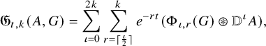 $$ \begin{align} \mathfrak{G}_{t,k}(A,G)=\sum_{\iota=0}^{2k}\sum_{r=\lceil \frac{\iota}{2} \rceil}^{k} e^{-rt}(\Phi_{\iota,r}(G)\circledast {\mathbb{D}}^\iota A), \end{align} $$
where here and in the rest,
 $\circledast $
denotes some tensorial contraction, and we have
$\circledast $
denotes some tensorial contraction, and we have
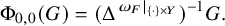 $$ \begin{align} \Phi_{0,0}(G)=(\Delta^{\omega_F|_{\{\cdot\}\times Y}})^{-1}G. \end{align} $$
For all
 $i<j$
, we suppose that we have smooth functions
$i<j$
, we suppose that we have smooth functions
 $G_{i,p,k}\in C^\infty (B\times Y,\mathbb {R}), 1\leqslant p\leqslant N_{i,k}$
, which have fiberwise average zero and are fiberwise
$G_{i,p,k}\in C^\infty (B\times Y,\mathbb {R}), 1\leqslant p\leqslant N_{i,k}$
, which have fiberwise average zero and are fiberwise
 $L^2$
orthonormal, with
$L^2$
orthonormal, with
 $G_{i,p,k}=0$
when
$G_{i,p,k}=0$
when
 $i=0$
. The main goal is to find smooth functions
$i=0$
. The main goal is to find smooth functions
 $G_{j,p,k}$
which satisfy a certain property that we now describe.
$G_{j,p,k}$
which satisfy a certain property that we now describe.
We are also given sequences of real numbers
 $t_{\ell }\to +\infty $
and
$t_{\ell }\to +\infty $
and
 $\delta _{\ell }>0$
with
$\delta _{\ell }>0$
with
 $\delta _{\ell }\to 0$
and
$\delta _{\ell }\to 0$
and
 $\lambda _{\ell }:=\delta _{\ell } e^{\frac {t_{\ell }}{2}}\to +\infty $
. Consider the diffeomorphisms
$\lambda _{\ell }:=\delta _{\ell } e^{\frac {t_{\ell }}{2}}\to +\infty $
. Consider the diffeomorphisms
 $$ \begin{align} \Sigma_{\ell}: B_{e^{\frac{t_{\ell}}{2}}} \times Y\times [-e^{t_{\ell}}t_{\ell},0] \to B \times Y\times [0,t_{\ell}], \;\, (z,y,t) = \Sigma_{\ell}(\check{z},\check{y},\check{t}) =(e^{-\frac{t_{\ell}}{2}}\check{z},\check{y},t_{\ell}+e^{-t_{\ell}}\check{t}), \end{align} $$
where
 $B_R:=B_{\mathbb {C}^m}(0,R)$
, and for any function u on
$B_R:=B_{\mathbb {C}^m}(0,R)$
, and for any function u on
 $B\times Y\times [0,t_{\ell }]$
, we will write
$B\times Y\times [0,t_{\ell }]$
, we will write
 $\check {u}_{\ell }=\Sigma _{\ell }^{*}u$
, and for a time-dependent
$\check {u}_{\ell }=\Sigma _{\ell }^{*}u$
, and for a time-dependent
 $2$
-form
$2$
-form
 $\alpha $
(with
$\alpha $
(with
 $t\in [0,t_{\ell }]$
) we will write
$t\in [0,t_{\ell }]$
) we will write
 $\check {\alpha }_{\ell }=e^{t_{\ell }}\Sigma _{\ell }^{*}\alpha $
. In particular, note that
$\check {\alpha }_{\ell }=e^{t_{\ell }}\Sigma _{\ell }^{*}\alpha $
. In particular, note that
 $\check {\omega }_{\ell , \mathrm {can}}=e^{t_{\ell }}\Sigma _{\ell }^{*}\omega _{\mathrm {can}}$
is a (time-independent) Kähler metric on
$\check {\omega }_{\ell , \mathrm {can}}=e^{t_{\ell }}\Sigma _{\ell }^{*}\omega _{\mathrm {can}}$
is a (time-independent) Kähler metric on
 $B_{e^{\frac {t_{\ell }}{2}}}$
uniformly equivalent to Euclidean (independent of
$B_{e^{\frac {t_{\ell }}{2}}}$
uniformly equivalent to Euclidean (independent of
 $\ell $
).
$\ell $
).
We will also need to factor
 $\Sigma _{\ell } = \Psi _{\ell }\circ \Xi _{\ell }$
, where
$\Sigma _{\ell } = \Psi _{\ell }\circ \Xi _{\ell }$
, where
 $$ \begin{align} \Xi_{\ell}: B_{e^{\frac{t_{\ell}}{2}}} \times Y\times [-e^{t_{\ell}}t_{\ell},0] \to B_{\lambda_{\ell}} \times Y\times [-\lambda_{\ell}^2t_{\ell},0], \;\, (\hat{z},\hat{y},\hat{t}) = \Xi_{\ell}(\check{z},\check{y},\check{t}) =(\delta_{\ell}\check{z},\check{y},\delta_{\ell}^2\check{t}), \end{align} $$
 $$ \begin{align} \Psi_{\ell}: B_{\lambda_{\ell}} \times Y\times [-\lambda_{\ell}^2t_{\ell},0] \to B \times Y\times [0,t_{\ell}], \;\, (z,y,t) = \Psi_{\ell}(\hat{z},\hat{y},\hat{t}) =(\lambda_{\ell}^{-1}\hat{z},\hat{y},t_{\ell}+\lambda_{\ell}^{-2}\hat{t}), \end{align} $$
and given a function u on
 $B\times Y\times [0,t_{\ell }]$
, we will write
$B\times Y\times [0,t_{\ell }]$
, we will write
 $\hat {u}=\Psi _{\ell }^{*}u$
, and given a time-dependent
$\hat {u}=\Psi _{\ell }^{*}u$
, and given a time-dependent
 $2$
-form
$2$
-form
 $\alpha $
, we will write
$\alpha $
, we will write
 $\hat {\alpha }=\lambda _{\ell }^2\Psi _{\ell }^{*}\alpha $
. We will also use the notation
$\hat {\alpha }=\lambda _{\ell }^2\Psi _{\ell }^{*}\alpha $
. We will also use the notation
 $$ \begin{align} \hat{Q}_R:=B_R\times Y\times [-R^2,0]\ni (\hat{z},\hat{y},\hat{t}), \quad \check{Q}_R:=B_R\times Y\times [-R^2,0]\ni (\check{z},\check{y},\check{t}), \end{align} $$
so that for example
 $\Xi _{\ell }(\check {Q}_R)=\hat {Q}_{R\delta _{\ell }^{-1}}$
.
$\Xi _{\ell }(\check {Q}_R)=\hat {Q}_{R\delta _{\ell }^{-1}}$
.
Let also
 $\eta ^\ddagger _{\ell }$
be an arbitrary sequence of
$\eta ^\ddagger _{\ell }$
be an arbitrary sequence of
 $(1,1)$
-forms on
$(1,1)$
-forms on
 $B\times [0, t_{\ell }]$
with coefficients (spacetime) polynomials of degree at most
$B\times [0, t_{\ell }]$
with coefficients (spacetime) polynomials of degree at most
 $2j$
which satisfy
$2j$
which satisfy
 $\hat {\eta }^\ddagger _{\ell }\to 0$
locally smoothly in spacetime (which implies that
$\hat {\eta }^\ddagger _{\ell }\to 0$
locally smoothly in spacetime (which implies that
 $\check {\eta }^\ddagger _{\ell }\to 0$
locally smoothly as well), let
$\check {\eta }^\ddagger _{\ell }\to 0$
locally smoothly as well), let
 $B^\sharp _{\ell }$
be an arbitrary sequence of smooth functions on
$B^\sharp _{\ell }$
be an arbitrary sequence of smooth functions on
 $B\times [0,t_{\ell }]$
such that
$B\times [0,t_{\ell }]$
such that
 $\hat {B}^\sharp _{\ell }\to 0$
locally smoothly, and for
$\hat {B}^\sharp _{\ell }\to 0$
locally smoothly, and for
 $1\leqslant i\leqslant j$
, let
$1\leqslant i\leqslant j$
, let
 $A^\sharp _{i,p,k}$
be arbitrary (spacetime) polynomials of degree at most
$A^\sharp _{i,p,k}$
be arbitrary (spacetime) polynomials of degree at most
 $2j$
on B such that
$2j$
on B such that
 $\hat {A}^\sharp _{\ell ,i,p,k}=\lambda _{\ell }^2\Psi _{\ell }^{*}A^\sharp _{i,p,k}$
satisfy that there is some
$\hat {A}^\sharp _{\ell ,i,p,k}=\lambda _{\ell }^2\Psi _{\ell }^{*}A^\sharp _{i,p,k}$
satisfy that there is some
 $0<\alpha _0<1$
such that given any
$0<\alpha _0<1$
such that given any
 $R>0$
, there is
$R>0$
, there is
 $C>0$
with
$C>0$
with
 $$ \begin{align} \|\mathfrak{D}^\iota \hat{A}_{\ell,i,p,k}^\sharp\|_{\infty,\hat Q_{R},\hat{g}_{\ell}(0)}\leqslant C \delta_{\ell}^2 e^{-\alpha_0\frac{t_{\ell}}{2}} \end{align} $$
for all
 $0\leqslant \iota \leqslant 2j$
, or equivalently that
$0\leqslant \iota \leqslant 2j$
, or equivalently that
 $\check {A}^\sharp _{\ell ,i,p,k}=e^{t_{\ell }}\Sigma _{\ell }^{*}A^\sharp _{i,p,k}=\delta _{\ell }^2\Xi _{\ell }^{*}\hat {A}^\sharp _{\ell ,i,p,k}$
satisfy
$\check {A}^\sharp _{\ell ,i,p,k}=e^{t_{\ell }}\Sigma _{\ell }^{*}A^\sharp _{i,p,k}=\delta _{\ell }^2\Xi _{\ell }^{*}\hat {A}^\sharp _{\ell ,i,p,k}$
satisfy
 $$ \begin{align} \|\mathfrak{D}^\iota \check{A}_{\ell,i,p,k}^\sharp\|_{\infty,\check Q_{R\delta_{\ell}^{-1}},\check g_{\ell}(0)}\leqslant C \delta_{\ell}^\iota e^{-\alpha_0\frac{t_{\ell}}{2}}. \end{align} $$
With these, we define for
 $1\leqslant i\leqslant j$
 $$ \begin{align} \gamma^{\sharp}_{t,i,k}=\sum_{p=1}^{N_{i,k}}{i\partial\bar\partial}\mathfrak{G}_{t,k}(A^\sharp_{i,p,k},G_{i,p,k}), \end{align} $$
so
 $\gamma ^{\sharp }_{t,j,k}$
depends on how we choose the functions
$\gamma ^{\sharp }_{t,j,k}$
depends on how we choose the functions
 $G_{j,p,k}$
. It is proved by the argument in (4.200) below that our assumption (3.7) on
$G_{j,p,k}$
. It is proved by the argument in (4.200) below that our assumption (3.7) on
 $\hat {A}^\sharp _{\ell ,i,p,k}$
implies that for any
$\hat {A}^\sharp _{\ell ,i,p,k}$
implies that for any
 $R>0$
, there is
$R>0$
, there is
 $C>0$
with
$C>0$
with
 $$ \begin{align} \|\mathfrak{D}^\iota\hat{\gamma}^{\sharp}_{\ell,i,k}\|_{\infty,\hat{Q}_{R},\hat{g}_{\ell}(0)}\leqslant C\delta_{\ell}^{-\iota}e^{-\alpha_0 \frac{t_{\ell}}{2}}, \end{align} $$
or equivalently
 $$ \begin{align} \|\mathfrak{D}^\iota\check{\gamma}^{\sharp}_{\ell,i,k}\|_{\infty,\check Q_{R\delta_{\ell}^{-1}},\check g_{\ell}(0)}\leqslant Ce^{-\alpha_0 \frac{t_{\ell}}{2}}, \end{align} $$
for all
 $\iota \geqslant 0$
and all
$\iota \geqslant 0$
and all
 $1\leqslant i\leqslant j$
(these can be just taken as assumptions for now). Observe that the constants C in (3.10) and (3.11) depend on the choice of the functions
$1\leqslant i\leqslant j$
(these can be just taken as assumptions for now). Observe that the constants C in (3.10) and (3.11) depend on the choice of the functions
 $G_{j,p,k}$
, but the exponent
$G_{j,p,k}$
, but the exponent
 $\alpha _0$
does not. We also define
$\alpha _0$
does not. We also define
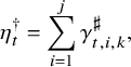 $$ \begin{align} \eta^\dagger_t=\sum_{i=1}^j\gamma^{\sharp}_{t,i,k}, \end{align} $$
and
 $$ \begin{align} \omega^\sharp_t=(1-e^{-t})\omega_{\mathrm{can}}+e^{-t}\omega_F+\eta^\dagger_t+\eta^\ddagger_t, \end{align} $$
which has the property that
 $\hat {\omega }^\sharp _{\ell }$
is a Kähler metric on
$\hat {\omega }^\sharp _{\ell }$
is a Kähler metric on
 $\hat {Q}_R$
for all
$\hat {Q}_R$
for all
 $R>0$
, and
$R>0$
, and
 $\ell $
sufficiently large, using that
$\ell $
sufficiently large, using that
 $\hat {\eta }^\ddagger _{\ell }$
is pulled back from B and goes to zero locally uniformly, and the estimate (3.10) with
$\hat {\eta }^\ddagger _{\ell }$
is pulled back from B and goes to zero locally uniformly, and the estimate (3.10) with
 $\iota =0$
for
$\iota =0$
for
 $\hat {\eta }^\dagger _{\ell }$
. Passing to the check picture, we obtain
$\hat {\eta }^\dagger _{\ell }$
. Passing to the check picture, we obtain
 $$ \begin{align} \check{\omega}^\sharp_{\ell}=(1-e^{-t_{\ell} -e^{-t_{\ell}}\check{t}})\check{\omega}_{\ell, \mathrm{ can}}+e^{-e^{-t_{\ell}}\check{t}}\Sigma_{\ell}^{*}\omega_F+\check{\eta}^\dagger_{\ell}+\check{\eta}^\ddagger_{\ell}. \end{align} $$
The key quantity we are interested in is then
 $$ \begin{align} \delta_{\ell}^{-2j-\alpha}\left(\log \frac{\binom{m+n}{n}\check\omega_{\ell,\mathrm{can}}^m\wedge (\Sigma_{\ell}^{*}\omega_F)^n}{(\check\omega_{\ell}^\sharp)^{m+n}} + \sum_{i=1}^j\sum_{p=1}^{N_{i,k}} \check{\mathfrak{G}}_{\check{t},k}( \partial_{\check{t}}{\check{A}}_{\ell,i,p,k}^\sharp+e^{-t_{\ell}}\check{A}_{\ell,i,p,k}^\sharp,\check G_{\ell,i,p,k}) +\Sigma_{\ell}^{*}B^\sharp_{\ell} \right), \end{align} $$
which can be compared to the corresponding quantity [Reference Hein and Tosatti21, (3.47)] in the elliptic setting. Observe that by definition, we have
 $\Sigma _{\ell }^{*}B^\sharp _{\ell }=\Xi _{\ell }^{*}\hat {B}^\sharp _{\ell }$
.
$\Sigma _{\ell }^{*}B^\sharp _{\ell }=\Xi _{\ell }^{*}\hat {B}^\sharp _{\ell }$
.
To clarify, when we will apply the Selection Theorem later, the functions
 $B^\sharp _{\ell }$
will be defined by
$B^\sharp _{\ell }$
will be defined by
 $$ \begin{align} \hat{B}^\sharp_{\ell}=e^{-\lambda_{\ell}^{-2}\hat{t}}\partial_{\hat{t}}\underline{{\hat{\chi}}_{\ell}^\sharp}-n\lambda_{\ell}^{-2}\hat{t}, \end{align} $$
where
 $\partial _{\hat {t}}\underline{{\hat {\chi }}_{\ell }^\sharp }$
is a spacetime polynomial of degree at most
$\partial _{\hat {t}}\underline{{\hat {\chi }}_{\ell }^\sharp }$
is a spacetime polynomial of degree at most
 $2j$
. The fact that
$2j$
. The fact that
 $\hat {B}^\sharp _{\ell }\to 0$
locally smoothly will follow from (4.158). We will also later define
$\hat {B}^\sharp _{\ell }\to 0$
locally smoothly will follow from (4.158). We will also later define
 $$ \begin{align} \underline{\check{\chi}}_{\ell}^\sharp=\delta_{\ell}^{-2}\Xi_{\ell}^{*}(\underline{{\hat{\chi}}_{\ell}^\sharp}). \end{align} $$
Hence, we will have
 $$ \begin{align} \Sigma_{\ell}^{*}B^\sharp_{\ell}=\Xi_{\ell}^{*}\hat{B}^\sharp_{\ell}=e^{-e^{-t_{\ell}}\check t}\partial_{\check t}\underline{\check\chi_{\ell}^\sharp}-ne^{-t_{\ell}}\check{t}. \end{align} $$
Given these preliminaries, the following is then the key result:
Theorem 3.1 (Selection Theorem)
Suppose we are given
 $0\leqslant j\leqslant k$
and when
$0\leqslant j\leqslant k$
and when
 $j>1$
, we are also given smooth function
$j>1$
, we are also given smooth function
 $G_{i,p,k},1\leqslant i\leqslant j-1,1\leqslant p\leqslant N_{i,k}$
, on
$G_{i,p,k},1\leqslant i\leqslant j-1,1\leqslant p\leqslant N_{i,k}$
, on
 $B\times Y$
which are fiberwise
$B\times Y$
which are fiberwise
 $L^2$
orthonormal and have fiberwise average zero. Then there are a concentric ball
$L^2$
orthonormal and have fiberwise average zero. Then there are a concentric ball
 $B'=B_{\mathbb {C}^m}(0,r)\subset B$
and smooth functions
$B'=B_{\mathbb {C}^m}(0,r)\subset B$
and smooth functions
 $G_{j,p,k},1\leqslant p\leqslant N_{j,k}$
on
$G_{j,p,k},1\leqslant p\leqslant N_{j,k}$
on
 $B'\times Y$
(identically zero if
$B'\times Y$
(identically zero if
 $j=0$
), with fiberwise average zero so that
$j=0$
), with fiberwise average zero so that
 $G_{i,p,k},1\leqslant p\leqslant N_{i,k},1\leqslant i\leqslant j$
are all fiberwise
$G_{i,p,k},1\leqslant p\leqslant N_{i,k},1\leqslant i\leqslant j$
are all fiberwise
 $L^2$
orthonormal with the following property: if
$L^2$
orthonormal with the following property: if
 $\delta _{\ell },t_{\ell }>0$
are any sequences with
$\delta _{\ell },t_{\ell }>0$
are any sequences with
 $t_{\ell }\to +\infty $
,
$t_{\ell }\to +\infty $
,
 $\delta _{\ell }\to 0$
and
$\delta _{\ell }\to 0$
and
 $\delta _{\ell } e^{\frac {t_{\ell }}{2}}\to +\infty ,$
and if
$\delta _{\ell } e^{\frac {t_{\ell }}{2}}\to +\infty ,$
and if
 $A_{i,p,k}^\sharp ,B^\sharp _{\ell },\eta _{\ell }^\dagger ,\eta _{\ell }^\ddagger ,\omega _{\ell }^\sharp $
are as above, and if (3.15) converges locally uniformly on
$A_{i,p,k}^\sharp ,B^\sharp _{\ell },\eta _{\ell }^\dagger ,\eta _{\ell }^\ddagger ,\omega _{\ell }^\sharp $
are as above, and if (3.15) converges locally uniformly on
 $\mathbb {C}^m\times Y\times (-\infty ,0]$
to some limiting function
$\mathbb {C}^m\times Y\times (-\infty ,0]$
to some limiting function
 $\mathcal {F}$
as
$\mathcal {F}$
as
 $\ell \to \infty $
, then on
$\ell \to \infty $
, then on
 $\Sigma _{\ell }^{-1}(B'\times Y\times [-r^2,0])$
, we can write (3.15) as
$\Sigma _{\ell }^{-1}(B'\times Y\times [-r^2,0])$
, we can write (3.15) as
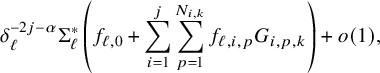 $$ \begin{align} \delta_{\ell}^{-2j-{\alpha}}\Sigma_{\ell}^{*}\left( f_{\ell,0}+\sum_{i=1}^j \sum_{p=1}^{N_{i,k}}f_{\ell,i,p} G_{i,p,k}\right)+o(1), \end{align} $$
where
 $f_{\ell ,0}, f_{\ell ,i,p}$
are functions pulled back from
$f_{\ell ,0}, f_{\ell ,i,p}$
are functions pulled back from
 $B'\times (-r^2,0]$
such that
$B'\times (-r^2,0]$
such that
 $\hat {f}_{\ell , 0}=\Psi _{\ell }^{*}f_{\ell ,0},\hat {f}_{\ell ,i,p}=\Psi _{\ell }^{*}f_{\ell ,i,p}$
converge locally smoothly to zero, and
$\hat {f}_{\ell , 0}=\Psi _{\ell }^{*}f_{\ell ,0},\hat {f}_{\ell ,i,p}=\Psi _{\ell }^{*}f_{\ell ,i,p}$
converge locally smoothly to zero, and
 $o(1)$
is a term that converges locally smoothly to zero. Lastly, (3.15) converges to
$o(1)$
is a term that converges locally smoothly to zero. Lastly, (3.15) converges to
 $\mathcal {F}$
locally smoothly.
$\mathcal {F}$
locally smoothly.
Remark 3.2. The argument follows closely the proof of the Selection Theorem 3.11 in [Reference Hein and Tosatti21], but apart from the obvious change from space to space-time, there are some other differences that we now briefly discuss, which arise from the different structure of the parabolic complex Monge-Ampère equation that we have compared to its elliptic counterpart in [Reference Hein and Tosatti21]. The first term in (3.15) is reminescent of [Reference Hein and Tosatti21, (3.47)], but it now has a logarithm. This change will be quite immaterial, since
 $\log (x)\approx x-1$
for
$\log (x)\approx x-1$
for
 $x\approx 1$
. Next, compared to [Reference Hein and Tosatti21, (3.47)], the quantity in (3.15) also contains two more pieces. The last term with
$x\approx 1$
. Next, compared to [Reference Hein and Tosatti21, (3.47)], the quantity in (3.15) also contains two more pieces. The last term with
 $B^\sharp _{\ell }$
is trivially acceptable since it can be absorbed into
$B^\sharp _{\ell }$
is trivially acceptable since it can be absorbed into
 $f_{\ell ,0}$
, while the term involving
$f_{\ell ,0}$
, while the term involving
 $\check {\mathfrak {G}}_{\check {t},k}$
will have to be dealt with, and it will turn out to be ‘lower order’ compared to the first term in (3.15). Putting these all together will allow us to follow the proof of [Reference Hein and Tosatti21, Theorem 3.11] very closely.
$\check {\mathfrak {G}}_{\check {t},k}$
will have to be dealt with, and it will turn out to be ‘lower order’ compared to the first term in (3.15). Putting these all together will allow us to follow the proof of [Reference Hein and Tosatti21, Theorem 3.11] very closely.
Proof. The proof is by induction on j. First, we treat the base case
 $j=0$
. In this case, by definition, there are no obstruction functions and the quantity in (3.15) reduces to
$j=0$
. In this case, by definition, there are no obstruction functions and the quantity in (3.15) reduces to
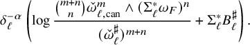 $$ \begin{align} \delta_{\ell}^{-\alpha}\left(\log \frac{\binom{m+n}{n}\check\omega_{\ell,\mathrm{can}}^m\wedge (\Sigma_{\ell}^{*}\omega_F)^n}{(\check\omega_{\ell}^\sharp)^{m+n}} +\Sigma_{\ell}^{*}B^\sharp_{\ell} \right). \end{align} $$
As in [Reference Hein and Tosatti21], we introduce the notation
 $$ \begin{align} \Sigma_{\ell}^{*}\omega_F=(\Sigma_{\ell}^{*}\omega_F)_{\mathbf{bb}}+(\Sigma_{\ell}^{*}\omega_F)_{\mathbf{bf}}+(\Sigma_{\ell}^{*}\omega_F)_{\mathbf{ff}}=: e^{-t_{\ell}}\check\omega_{F,\mathbf{bb}}+e^{-\frac{t_{\ell}}{2}}\check\omega_{F,\mathbf{bf}}+\check\omega_{F,\mathbf{ff}}, \end{align} $$
where the functions
 $\check \omega _{F,\mathbf {bb}},\check \omega _{F,\mathbf {bf}},\check \omega _{F,\mathbf {ff}}$
so defined are uniformly bounded on
$\check \omega _{F,\mathbf {bb}},\check \omega _{F,\mathbf {bf}},\check \omega _{F,\mathbf {ff}}$
so defined are uniformly bounded on
 $B_{e^{\frac {t_{\ell }}{2}}}\times Y\times [-e^{t_{\ell }}t_{\ell },0]$
. Following [Reference Hein and Tosatti21, (3.50)], we then compute
$B_{e^{\frac {t_{\ell }}{2}}}\times Y\times [-e^{t_{\ell }}t_{\ell },0]$
. Following [Reference Hein and Tosatti21, (3.50)], we then compute
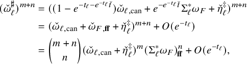 $$ \begin{align}\begin{aligned} (\check\omega_{\ell}^\sharp)^{m+n}&=((1-e^{-t_{\ell} -e^{-t_{\ell}}\check{t}})\check{\omega}_{\ell, \mathrm{ can}}+e^{-e^{-t_{\ell}}\check{t}}\Sigma_{\ell}^{*}\omega_F+\check{\eta}^\ddagger_{\ell})^{m+n}\\ &=(\check{\omega}_{\ell, \mathrm{ can}}+\check\omega_{F,\mathbf{ff}}+\check{\eta}^\ddagger_{\ell})^{m+n}+O(e^{-{t_{\ell}}})\\ &=\binom{m+n}{n}(\check{\omega}_{\ell, \mathrm{ can}}+\check{\eta}^\ddagger_{\ell})^{m}(\Sigma_{\ell}^{*}\omega_F)_{\mathbf{ff}}^n+O(e^{-{t_{\ell}}}), \end{aligned}\end{align} $$
where the
 $O(e^{-t_{\ell }})$
is in the locally smooth topology, and so
$O(e^{-t_{\ell }})$
is in the locally smooth topology, and so
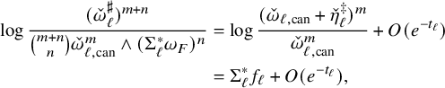 $$ \begin{align}\begin{aligned} \log \frac{(\check\omega_{\ell}^\sharp)^{m+n}}{\binom{m+n}{n}\check\omega_{\ell,\mathrm{can}}^m\wedge (\Sigma_{\ell}^{*}\omega_F)^n}&=\log\frac{(\check{\omega}_{\ell, \mathrm{ can}}+\check{\eta}^\ddagger_{\ell})^{m}}{\check\omega_{\ell,\mathrm{can}}^m}+O(e^{-t_{\ell}})\\ &=\Sigma_{\ell}^{*}f_{\ell}+ O(e^{-{t_{\ell}}}), \end{aligned}\end{align} $$
where
 $f_{\ell }$
is some sequence of smooth functions pulled back from B. Passing to the hat picture (i.e., letting
$f_{\ell }$
is some sequence of smooth functions pulled back from B. Passing to the hat picture (i.e., letting
 $\hat {f}_{\ell }=\Psi _{\ell }^{*}f_{\ell }$
), our assumption that
$\hat {f}_{\ell }=\Psi _{\ell }^{*}f_{\ell }$
), our assumption that
 $\hat {\eta }^\ddagger _{\ell }\to 0$
locally smoothly implies that
$\hat {\eta }^\ddagger _{\ell }\to 0$
locally smoothly implies that
 $\hat {f}_{\ell }\to 0$
locally smoothly. It thus follows that
$\hat {f}_{\ell }\to 0$
locally smoothly. It thus follows that
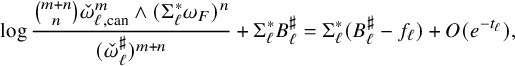 $$ \begin{align} \log \frac{\binom{m+n}{n}\check\omega_{\ell,\mathrm{can}}^m\wedge (\Sigma_{\ell}^{*}\omega_F)^n}{(\check\omega_{\ell}^\sharp)^{m+n}}+\Sigma_{\ell}^{*}B^\sharp_{\ell}=\Sigma_{\ell}^{*}(B^\sharp_{\ell}-f_{\ell})+O(e^{-{t_{\ell}}}),\end{align} $$
and recalling that
 $\hat {f}_{\ell }\to 0$
and
$\hat {f}_{\ell }\to 0$
and
 $\hat {B}^\sharp _{\ell }\to 0$
locally smoothly, as well as
$\hat {B}^\sharp _{\ell }\to 0$
locally smoothly, as well as
 $\delta _{\ell }^{-\alpha }e^{-{t_{\ell }}}=o(1)$
, we see that (3.19) holds. Lastly, since by assumption (3.20) converges locally uniformly to
$\delta _{\ell }^{-\alpha }e^{-{t_{\ell }}}=o(1)$
, we see that (3.19) holds. Lastly, since by assumption (3.20) converges locally uniformly to
 $\mathcal {F}$
, the same is true for
$\mathcal {F}$
, the same is true for
 $\delta _{\ell }^{-\alpha }\Sigma _{\ell }^{*}(B^\sharp _{\ell }-f_{\ell })$
, and the same argument as in [Reference Hein and Tosatti21, (3.52)–(3.54)] shows that this convergence is locally smooth. This concludes the proof of Theorem 3.1 in the case
$\delta _{\ell }^{-\alpha }\Sigma _{\ell }^{*}(B^\sharp _{\ell }-f_{\ell })$
, and the same argument as in [Reference Hein and Tosatti21, (3.52)–(3.54)] shows that this convergence is locally smooth. This concludes the proof of Theorem 3.1 in the case
 $j=0$
.
$j=0$
.
We then treat the inductive step, and assume
 $j\geqslant 1$
. By assumption, the obstruction functions
$j\geqslant 1$
. By assumption, the obstruction functions
 $G_{i,p,k}$
with
$G_{i,p,k}$
with
 $1\leqslant i<j$
have already been selected on
$1\leqslant i<j$
have already been selected on
 $B'\times Y$
(recall that
$B'\times Y$
(recall that
 $B'=B_r$
), and we need to select the
$B'=B_r$
), and we need to select the
 $G_{j,p,k}$
’s. As in [Reference Hein and Tosatti21], this will be done via an iterative procedure, with iteration parameter
$G_{j,p,k}$
’s. As in [Reference Hein and Tosatti21], this will be done via an iterative procedure, with iteration parameter
 $\kappa $
, initially set at
$\kappa $
, initially set at
 $\kappa =0$
, and at each step assuming we have already selected some obstruction functions
$\kappa =0$
, and at each step assuming we have already selected some obstruction functions
 $G^{[q]}_{j,p,k}, 1\leqslant q\leqslant \kappa $
(this being the empty list when
$G^{[q]}_{j,p,k}, 1\leqslant q\leqslant \kappa $
(this being the empty list when
 $\kappa =0$
), and with the iterative step consisting of selecting some new obstruction functions
$\kappa =0$
), and with the iterative step consisting of selecting some new obstruction functions
 $G^{[\kappa +1]}_{j,p,k}$
to add to these. After this will be achieved, we will then show that if we perform this iterative step
$G^{[\kappa +1]}_{j,p,k}$
to add to these. After this will be achieved, we will then show that if we perform this iterative step
 $\overline {\kappa }$
times (for some uniform
$\overline {\kappa }$
times (for some uniform
 $\overline {\kappa }$
) and define the obstruction function
$\overline {\kappa }$
) and define the obstruction function
 $G_{j,p,k}$
by putting together all the
$G_{j,p,k}$
by putting together all the
 $G^{[q]}_{j,p,k}$
’s obtained at all iterations
$G^{[q]}_{j,p,k}$
’s obtained at all iterations
 $1\leqslant q\leqslant \overline {\kappa }+1$
, then the desired conclusion (3.19) holds.
$1\leqslant q\leqslant \overline {\kappa }+1$
, then the desired conclusion (3.19) holds.
To start the proof, we give a couple of definitions following [Reference Hein and Tosatti21]. We will say that a sequence of functions on
 $\Sigma _{\ell }^{-1}(B_r\times Y\times (-r^2,0])$
satisfies condition
$\Sigma _{\ell }^{-1}(B_r\times Y\times (-r^2,0])$
satisfies condition
 $(\star )$
if it equals
$(\star )$
if it equals
 $$ \begin{align} \delta_{\ell}^{-2j-\alpha}\Sigma_{\ell}^{*}\left(f_{\ell,0}+\sum_{i=1}^N f_{\ell,i}h_i\right) + o(1) \end{align} $$
for some
 $N\in \mathbb {N}$
, where the functions
$N\in \mathbb {N}$
, where the functions
 $f_{\ell ,0},f_{\ell ,i}$
are smooth and pulled back from
$f_{\ell ,0},f_{\ell ,i}$
are smooth and pulled back from
 $B_r\times (-r^2,0]$
and
$B_r\times (-r^2,0]$
and
 $\hat {f}_{\ell ,0}=\Psi _{\ell }^{*}f_{\ell ,0}, \hat {f}_{\ell ,i}=\Psi _{\ell }^{*}f_{\ell ,i}$
converge locally smoothly to zero, the time-independent functions
$\hat {f}_{\ell ,0}=\Psi _{\ell }^{*}f_{\ell ,0}, \hat {f}_{\ell ,i}=\Psi _{\ell }^{*}f_{\ell ,i}$
converge locally smoothly to zero, the time-independent functions
 $h_i$
are smooth on
$h_i$
are smooth on
 $B_r\times Y$
with fiberwise average zero, and the
$B_r\times Y$
with fiberwise average zero, and the
 $o(1)$
is a term that converges locally smoothly to zero. This definition is tailored to our desired conclusion in (3.19). As in [Reference Hein and Tosatti21, Remark 3.13], we see that if a sequence of functions satisfies
$o(1)$
is a term that converges locally smoothly to zero. This definition is tailored to our desired conclusion in (3.19). As in [Reference Hein and Tosatti21, Remark 3.13], we see that if a sequence of functions satisfies
 $(\star )$
and converges locally uniformly to some limit, then this convergence is actually smooth.
$(\star )$
and converges locally uniformly to some limit, then this convergence is actually smooth.
For
 $\kappa \geqslant 0$
, given also arbitrary spacetime polynomials
$\kappa \geqslant 0$
, given also arbitrary spacetime polynomials
 $A^{\sharp ,[q]}_{j,p,k},1\leqslant q\leqslant \kappa ,$
of degree at most
$A^{\sharp ,[q]}_{j,p,k},1\leqslant q\leqslant \kappa ,$
of degree at most
 $2j$
such that
$2j$
such that
 $\check {A}^{\sharp ,[q]}_{\ell ,j,p,k}=e^{t_{\ell }}\Sigma _{\ell }^{*}A^{\sharp ,[q]}_{j,p,k}$
satisfy (3.8), we construct as in (3.9)
$\check {A}^{\sharp ,[q]}_{\ell ,j,p,k}=e^{t_{\ell }}\Sigma _{\ell }^{*}A^{\sharp ,[q]}_{j,p,k}$
satisfy (3.8), we construct as in (3.9)
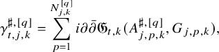 $$ \begin{align} \gamma^{\sharp,[q]}_{t,j,k}=\sum_{p=1}^{N_{j,k}^{[q]}}{i\partial\bar\partial}\mathfrak{G}_{t,k}(A^{\sharp,[q]}_{j,p,k},G_{j,p,k}), \end{align} $$
for
 $1\leqslant q\leqslant \kappa $
(setting
$1\leqslant q\leqslant \kappa $
(setting
 $\gamma ^{\sharp ,[0]}_{t,j,k}=0$
) and let
$\gamma ^{\sharp ,[0]}_{t,j,k}=0$
) and let
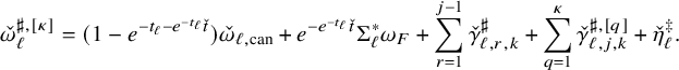 $$ \begin{align} \check{\omega}^{\sharp,[\kappa]}_{\ell}=(1-e^{-t_{\ell} -e^{-t_{\ell}}\check{t}})\check{\omega}_{\ell, \mathrm{ can}}+e^{-e^{-t_{\ell}}\check{t}}\Sigma_{\ell}^{*}\omega_F+\sum_{r=1}^{j-1}\check{\gamma}^{\sharp}_{\ell,r,k}+ \sum_{q=1}^\kappa\check{\gamma}^{\sharp,[q]}_{\ell,j,k}+\check{\eta}^\ddagger_{\ell}. \end{align} $$
This is a Kähler metric on
 $B_r\times Y\times (-r^2,0]$
, and we can then consider the function
$B_r\times Y\times (-r^2,0]$
, and we can then consider the function
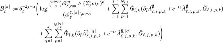 $$ \begin{align}\begin{aligned} \mathcal{B}_{\ell}^{[\kappa]}:=\delta_{\ell}^{-2j-\alpha}\bigg(&\log \frac{\binom{m+n}{n}\check\omega_{\ell,\mathrm{can}}^m\wedge (\Sigma_{\ell}^{*}\omega_F)^n}{(\check\omega_{\ell}^{\sharp,[\kappa]})^{m+n}} + \sum_{i=1}^{j-1}\sum_{p=1}^{N_{i,k}} \check{\mathfrak{G}}_{\check{t},k}( \partial_{\check{t}}{\check{A}}_{\ell,i,p,k}^\sharp+e^{-t_{\ell}}\check{A}_{\ell,i,p,k}^\sharp,\check G_{\ell,i,p,k})\\ &+\sum_{q=1}^{\kappa}\sum_{p=1}^{N_{j,k}^{[q]}} \check{\mathfrak{G}}_{\check{t},k}( \partial_{\check{t}}{\check{A}}^{\sharp,[q]}_{\ell,j,p,k}+e^{-t_{\ell}}\check{A}^{\sharp,[q]}_{\ell,j,p,k},\check G_{\ell,j,p,k}) \bigg). \end{aligned}\end{align} $$
The following is the analog of [Reference Hein and Tosatti21, Lemma 3.14]:
Lemma 3.3. Suppose either
 $\kappa =0$
or
$\kappa =0$
or
 $\kappa \geqslant 1$
and we have selected the functions
$\kappa \geqslant 1$
and we have selected the functions
 $G_{j,p,k}^{[q]}$
as above for
$G_{j,p,k}^{[q]}$
as above for
 $1\leqslant q\leqslant \kappa .$
Then the sequence of functions
$1\leqslant q\leqslant \kappa .$
Then the sequence of functions
 $\mathcal {B}_{\ell }^{[\kappa ]}$
satisfies
$\mathcal {B}_{\ell }^{[\kappa ]}$
satisfies
 $(\star )$
. Furthermore, we have
$(\star )$
. Furthermore, we have
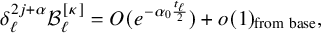 $$ \begin{align} \delta_{\ell}^{2j+\alpha}\mathcal{B}_{\ell}^{[\kappa]}=O(e^{-\alpha_0\frac{t_{\ell}}{2}})+o(1)_{\mathrm{from\ base}}, \end{align} $$
where the term
 $O(e^{-\alpha _0\frac {t_{\ell }}{2}})$
is in
$O(e^{-\alpha _0\frac {t_{\ell }}{2}})$
is in
 $L^\infty _{\mathrm {loc}}$
, while the last term is a function from the base which goes to zero locally smoothly.
$L^\infty _{\mathrm {loc}}$
, while the last term is a function from the base which goes to zero locally smoothly.
Proof. For ease of notation, define
 $$ \begin{align} \omega^\square_t=(1-e^{-t})\omega_{\mathrm{can}}+e^{-t}\omega_F+\eta^\ddagger_t, \end{align} $$
which have the property that
 $\hat {\omega }^\square _{\ell }$
are Kähler metrics on
$\hat {\omega }^\square _{\ell }$
are Kähler metrics on
 $\hat {Q}_R$
for all
$\hat {Q}_R$
for all
 $R>0$
and
$R>0$
and
 $\ell $
large, and which in the check picture become
$\ell $
large, and which in the check picture become
 $$ \begin{align} \check{\omega}^\square_{\ell}=(1-e^{-t_{\ell} -e^{-t_{\ell}}\check{t}})\check{\omega}_{\ell, \mathrm{ can}}+e^{-e^{-t_{\ell}}\check{t}}\Sigma_{\ell}^{*}\omega_F+\check{\eta}^\ddagger_{\ell}. \end{align} $$
We first consider (in the original undecorated picture)
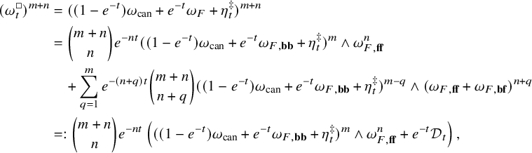 $$ \begin{align}\begin{aligned} (\omega^\square_t)^{m+n}&=((1-e^{-t})\omega_{\mathrm{can}}+e^{-t}\omega_F+\eta^\ddagger_t)^{m+n}\\&=\binom{m+n}{n}e^{-nt}((1-e^{-t})\omega_{\mathrm{can}}+e^{-t}\omega_{F,\mathbf{bb}}+\eta^\ddagger_t)^m\wedge\omega_{F,\mathbf{ff}}^n\\&\quad +\sum_{q=1}^me^{-(n+q)t}\binom{m+n}{n+q}((1-e^{-t})\omega_{\mathrm{can}}+e^{-t}\omega_{F,\mathbf{bb}}+\eta^\ddagger_t)^{m-q}\wedge(\omega_{F,\mathbf{ff}}+\omega_{F,\mathbf{bf}})^{n+q}\\&=:\binom{m+n}{n}e^{-nt}\left(((1-e^{-t})\omega_{\mathrm{can}}+e^{-t}\omega_{F,\mathbf{bb}}+\eta^\ddagger_t)^m\wedge\omega_{F,\mathbf{ff}}^n+e^{-t}\mathcal{D}_t\right), \end{aligned} \end{align} $$
and so
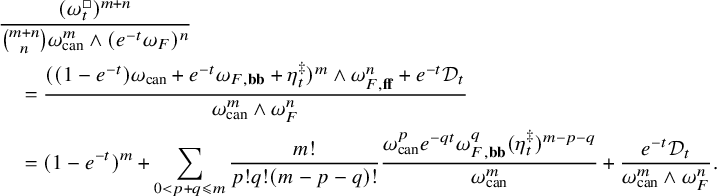 $$ \begin{align}\begin{aligned} &\frac{(\omega^\square_t)^{m+n}}{\binom{m+n}{n}\omega_{\mathrm{can}}^m\wedge (e^{-t}\omega_F)^n}\\&\quad =\frac{((1-e^{-t})\omega_{\mathrm{can}}+e^{-t}\omega_{F,\mathbf{bb}}+\eta^\ddagger_t)^m\wedge\omega_{F,\mathbf{ff}}^n+e^{-t}\mathcal{D}_t}{\omega_{\mathrm{can}}^m\wedge \omega_F^n}\\&\quad =(1-e^{-t})^m+\sum_{0<p+q\leqslant m}\frac{m!}{p!q!(m-p-q)!}\frac{\omega_{\mathrm{can}}^pe^{-qt}\omega^q_{F,\mathbf{bb}}(\eta_t^\ddagger)^{m-p-q}}{\omega_{\mathrm{can}}^m} +\frac{e^{-t}\mathcal{D}_t}{\omega_{\mathrm{can}}^m\wedge \omega_F^n}. \end{aligned}\end{align} $$
Note that the functions
 $$ \begin{align} \frac{\omega_{\mathrm{can}}^{p}e^{-qt}\omega_{F,\mathbf{bb}}^q(\eta^\ddagger_t)^{m-p-q}}{\omega_{\mathrm{can}}^m} \end{align} $$
with
 $q=0$
are
$q=0$
are
 $o(1)$
and pulled back from B, while when
$o(1)$
and pulled back from B, while when
 $q>0$
they are not pulled back from B, but they are visibly of the form
$q>0$
they are not pulled back from B, but they are visibly of the form
 $f_{t,0}+\sum _{i=1}^N f_{t,i}h_i$
with the same notation as above, where the
$f_{t,0}+\sum _{i=1}^N f_{t,i}h_i$
with the same notation as above, where the
 $\hat {f}_{t,0},\hat {f}_{t,i}$
converge smoothly to zero at least as
$\hat {f}_{t,0},\hat {f}_{t,i}$
converge smoothly to zero at least as
 $O(e^{-qt})$
, and the functions
$O(e^{-qt})$
, and the functions
 $h_i$
have fiberwise average zero and do not depend on the choice of
$h_i$
have fiberwise average zero and do not depend on the choice of
 $\eta ^\ddagger _t$
. An analogous statement holds for
$\eta ^\ddagger _t$
. An analogous statement holds for
 $$ \begin{align} \frac{e^{-t}\mathcal{D}_t}{\omega_{\mathrm{can}}^m\wedge \omega_F^n}, \end{align} $$
and if we take the logarithm and use the Taylor expansion of
 $\log (1+x)$
, this shows that
$\log (1+x)$
, this shows that
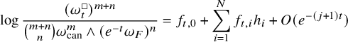 $$ \begin{align} \log\frac{(\omega^\square_t)^{m+n}}{\binom{m+n}{n}\omega_{\mathrm{can}}^m\wedge (e^{-t}\omega_F)^n}=f_{t,0}+\sum_{i=1}^N f_{t,i}h_i+O(e^{-(j+1)t}) \end{align} $$
for some possibly different functions
 $f_{t,0}, f_{t,i}$
, and where the term
$f_{t,0}, f_{t,i}$
, and where the term
 $O(e^{-(j+1)t})$
is in
$O(e^{-(j+1)t})$
is in
 $C^p_{\mathrm {loc}}$
for all
$C^p_{\mathrm {loc}}$
for all
 $p\geqslant 0$
. Passing to the check picture, we have
$p\geqslant 0$
. Passing to the check picture, we have
 $$ \begin{align} \log\frac{(\check{\omega}^\square_{\ell})^{m+n}}{\binom{m+n}{n}\check\omega_{\ell,\mathrm{can}}^m\wedge (\Sigma_{\ell}^{*}\omega_F)^n}=-ne^{-t_{\ell}}\check{t}+\Sigma_{\ell}^{*}\log\frac{((1-e^{-t})\omega_{\mathrm{ can}}+e^{-t}\omega_F+\eta^\ddagger_t)^{m+n}}{\binom{m+n}{n}\omega_{\mathrm{can}}^m\wedge (e^{-t}\omega_F)^n}, \end{align} $$
and so
 $$ \begin{align} \delta_{\ell}^{-2j-\alpha}\log\frac{(\check{\omega}^\square_{\ell})^{m+n}}{\binom{m+n}{n}\check\omega_{\ell,\mathrm{can}}^m\wedge (\Sigma_{\ell}^{*}\omega_F)^n}=\delta_{\ell}^{-2j-\alpha}\Sigma_{\ell}^{*}\left(f_{\ell,0}+\sum_{i=1}^N f_{\ell,i}h_i\right)+O(\delta_{\ell}^{-2j-\alpha}e^{-(j+1)t_{\ell}}), \end{align} $$
and
 $\delta _{\ell }^{-2j-\alpha }e^{-(j+1)t_{\ell }}=o(1)$
by assumption, namely the LHS of (3.38) satisfies
$\delta _{\ell }^{-2j-\alpha }e^{-(j+1)t_{\ell }}=o(1)$
by assumption, namely the LHS of (3.38) satisfies
 $(\star )$
, as well as
$(\star )$
, as well as
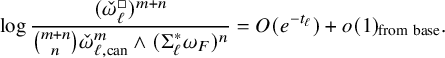 $$ \begin{align} \log\frac{(\check{\omega}^\square_{\ell})^{m+n}}{\binom{m+n}{n}\check\omega_{\ell,\mathrm{can}}^m\wedge (\Sigma_{\ell}^{*}\omega_F)^n}=O(e^{-t_{\ell}})+o(1)_{\mathrm{from\ base}}. \end{align} $$
The next step is to show that the quantity
 $$ \begin{align}\begin{aligned} \delta_{\ell}^{-2j-\alpha}\log \frac{(\check\omega_{\ell}^{\sharp,[\kappa]})^{m+n}}{\binom{m+n}{n}\check\omega_{\ell,\mathrm{can}}^m\wedge (\Sigma_{\ell}^{*}\omega_F)^n} = \delta_{\ell}^{-2j-\alpha} \log\frac{(\check{\omega}^\square_{\ell})^{m+n}}{\binom{m+n}{n}\check\omega_{\ell,\mathrm{can}}^m\wedge (\Sigma_{\ell}^{*}\omega_F)^n} +\delta_{\ell}^{-2j-\alpha}\log \frac{(\check\omega_{\ell}^{\sharp,[\kappa]})^{m+n}}{(\check{\omega}^\square_{\ell})^{m+n}} \end{aligned} \end{align} $$
also satisfies
 $(\star )$
. We have just discussed the first piece, and the second piece equals
$(\star )$
. We have just discussed the first piece, and the second piece equals
 $$ \begin{align}\begin{aligned} \delta_{\ell}^{-2j-\alpha}\log \left(1+\sum_{i=1}^{m+n}\binom{m+n}{i}\frac{(\check{\gamma}^\sharp_{\ell,1,k}+\cdots+\check{\gamma}^\sharp_{\ell,j-1,k}+ \check{\gamma}^{\sharp,[1]}_{\ell,j,k}+\cdots+\check{\gamma}^{\sharp,[\kappa]}_{\ell,j,k})^i\wedge(\check{\omega}^\square_{\ell})^{m+n-i}}{(\check{\omega}^\square_{\ell})^{m+n}}\right), \end{aligned} \end{align} $$
and for the terms with
 $\check {\gamma }^\sharp _{\ell ,1,k}+\cdots +\check {\gamma }^\sharp _{\ell ,j-1,k}+\check {\gamma }^{\sharp ,[1]}_{\ell ,j,k}+\cdots +\check {\gamma }^{\sharp ,[\kappa ]}_{\ell ,j,k}$
, we recall from (3.9) and (3.26) that we have
$\check {\gamma }^\sharp _{\ell ,1,k}+\cdots +\check {\gamma }^\sharp _{\ell ,j-1,k}+\check {\gamma }^{\sharp ,[1]}_{\ell ,j,k}+\cdots +\check {\gamma }^{\sharp ,[\kappa ]}_{\ell ,j,k}$
, we recall from (3.9) and (3.26) that we have
 $$ \begin{align} \check{\gamma}^{\sharp}_{\ell,i,k}=\sum_{p=1}^{N_{i,k}}{i\partial\bar\partial}\check{\mathfrak{G}}_{\check{t},k}(\check{A}^\sharp_{\ell,i,p,k},\check{G}_{i,p,k}),\quad \check{\gamma}^{\sharp,[q]}_{\ell,j,k}=\sum_{p=1}^{N_{j,k}^{[q]}}{i\partial\bar\partial}\check{\mathfrak{G}}_{\check{t},k}(\check{A}^{\sharp,[q]}_{\ell,j,p,k},\check{G}_{j,p,k}), \end{align} $$
with the bounds (3.11), where the approximate Green operator
 $\check {\mathfrak {G}}_{\check {t},k}$
is given schematically by
$\check {\mathfrak {G}}_{\check {t},k}$
is given schematically by
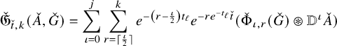 $$ \begin{align} \check{\mathfrak{G}}_{\check{t},k}(\check{A},\check{G}) = \sum_{\iota=0}^{j}\sum_{r=\lceil \frac{\iota}{2} \rceil}^{k} e^{-\left(r-\frac{\iota}{2}\right)t_{\ell}}e^{-re^{-t_{\ell}}\check{t}}(\check{\Phi}_{\iota,r}(\check{G})\circledast {\mathbb{D}}^\iota \check{A}) \end{align} $$
by (3.1). Plugging this into (3.41) and arguing as we did above reveals that the quantity in (3.40) satisfies
 $(\star )$
and that, furthermore,
$(\star )$
and that, furthermore,
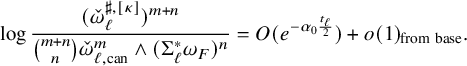 $$ \begin{align} \log \frac{(\check\omega_{\ell}^{\sharp,[\kappa]})^{m+n}}{\binom{m+n}{n}\check\omega_{\ell,\mathrm{can}}^m\wedge (\Sigma_{\ell}^{*}\omega_F)^n}=O(e^{-\alpha_0\frac{t_{\ell}}{2}})+o(1)_{\mathrm{from\ base}}. \end{align} $$
Lastly, to prove that
 $\mathcal {B}_{\ell }^{[\kappa ]}$
satisfies
$\mathcal {B}_{\ell }^{[\kappa ]}$
satisfies
 $(\star )$
, it remains to consider the piece
$(\star )$
, it remains to consider the piece
 $$ \begin{align} \delta_{\ell}^{-2j-\alpha}\left(\sum_{i=1}^{j-1}\sum_{p=1}^{N_{i,k}} \check{\mathfrak{G}}_{\check{t},k}( \partial_{\check{t}}{\check{A}}_{\ell,i,p,k}^\sharp+e^{-t_{\ell}}\check{A}_{\ell,i,p,k}^\sharp,\check G_{\ell,i,p,k}) +\sum_{q=1}^{\kappa}\sum_{p=1}^{N_{j,k}^{[q]}} \check{\mathfrak{G}}_{\check{t},k}( \partial_{\check{t}}{\check{A}}^{\sharp,[q]}_{\ell,j,p,k}+e^{-t_{\ell}}\check{A}^{\sharp,[q]}_{\ell,j,p,k},\check G_{\ell,j,p,k})\right). \end{align} $$
The fact that this term satisfies
 $(\star )$
again follows immediately from (3.43) together with (3.8), which also give that
$(\star )$
again follows immediately from (3.43) together with (3.8), which also give that
 $$ \begin{align}\begin{aligned} &\sum_{i=1}^{j-1}\sum_{p=1}^{N_{i,k}} \check{\mathfrak{G}}_{\check{t},k}( \partial_{\check{t}}{\check{A}}_{\ell,i,p,k}^\sharp+e^{-t_{\ell}}\check{A}_{\ell,i,p,k}^\sharp,\check G_{\ell,i,p,k}) +\sum_{q=1}^{\kappa}\sum_{p=1}^{N_{j,k}^{[q]}} \check{\mathfrak{G}}_{\check{t},k}( \partial_{\check{t}}{\check{A}}^{\sharp,[q]}_{\ell,j,p,k}+e^{-t_{\ell}}\check{A}^{\sharp,[q]}_{\ell,j,p,k},\check G_{\ell,j,p,k})\\&\quad= O(e^{-\alpha_0\frac{t_{\ell}}{2}})+o(1)_{\mathrm{from\ base}}, \end{aligned}\end{align} $$
and this completes the proof that
 $\mathcal {B}_{\ell }^{[\kappa ]}$
satisfies
$\mathcal {B}_{\ell }^{[\kappa ]}$
satisfies
 $(\star )$
and that (3.29) holds.
$(\star )$
and that (3.29) holds.
Now that Lemma 3.3 is established, we can start the first step of the iteration, when
 $\kappa =0$
and we need to select the obstruction functions
$\kappa =0$
and we need to select the obstruction functions
 $G^{[1]}_{j,p,k}$
. To do this, we consider
$G^{[1]}_{j,p,k}$
. To do this, we consider
 $\mathcal {B}_{\ell }^{[0]}$
, which by Lemma 3.3 satisfies
$\mathcal {B}_{\ell }^{[0]}$
, which by Lemma 3.3 satisfies
 $(\star )$
, and let
$(\star )$
, and let
 $\{h_i\}$
be the corresponding functions in its expansion (3.25). Applying the approximate fiberwise Gram-Schmidt [Reference Hein and Tosatti21, Proposition 3.1] to the functions
$\{h_i\}$
be the corresponding functions in its expansion (3.25). Applying the approximate fiberwise Gram-Schmidt [Reference Hein and Tosatti21, Proposition 3.1] to the functions
 $h_i$
together with the
$h_i$
together with the
 $G_{i,p,k}, 1\leqslant i<j$
, produces our desired list
$G_{i,p,k}, 1\leqslant i<j$
, produces our desired list
 $G^{[1]}_{j,p,k}$
(on
$G^{[1]}_{j,p,k}$
(on
 $B_r\times Y$
, up to shrinking r), so that we may assume that the functions
$B_r\times Y$
, up to shrinking r), so that we may assume that the functions
 $h_i$
in (3.25) lie in the fiberwise linear span of the
$h_i$
in (3.25) lie in the fiberwise linear span of the
 $G_{i,p,k}, 1\leqslant i<j$
together with the
$G_{i,p,k}, 1\leqslant i<j$
together with the
 $G^{[1]}_{j,p,k}$
. This completes the first step (
$G^{[1]}_{j,p,k}$
. This completes the first step (
 $\kappa =0$
).
$\kappa =0$
).
Next, we consider a subsequent step
 $\kappa \geqslant 1$
of the iteration, so we assume we are given the lists
$\kappa \geqslant 1$
of the iteration, so we assume we are given the lists
 $G_{i,p,k}, 1\leqslant i<j$
and
$G_{i,p,k}, 1\leqslant i<j$
and
 $G^{[q]}_{j,p,k}, 1\leqslant q\leqslant \kappa $
; hence, we have the function
$G^{[q]}_{j,p,k}, 1\leqslant q\leqslant \kappa $
; hence, we have the function
 $\mathcal {B}_{\ell }^{[\kappa ]}$
in (3.28), and we want to construct the obstruction functions
$\mathcal {B}_{\ell }^{[\kappa ]}$
in (3.28), and we want to construct the obstruction functions
 $G^{[\kappa +1]}_{j,p,k}$
. In order to do this, we must compare
$G^{[\kappa +1]}_{j,p,k}$
. In order to do this, we must compare
 $\mathcal {B}_{\ell }^{[\kappa ]}$
and
$\mathcal {B}_{\ell }^{[\kappa ]}$
and
 $\mathcal {B}_{\ell }^{[\kappa -1]}$
. We have
$\mathcal {B}_{\ell }^{[\kappa -1]}$
. We have
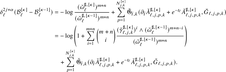 $$ \begin{align}\begin{aligned} \delta_{\ell}^{2j+\alpha}(\mathcal{B}_{\ell}^{[\kappa]}-\mathcal{B}_{\ell}^{[\kappa-1]})&=-\log\frac{(\check\omega_{\ell}^{\sharp,[\kappa]})^{m+n}}{(\check\omega_{\ell}^{\sharp,[\kappa-1]})^{m+n}} +\sum_{p=1}^{N_{j,k}^{[\kappa]}} \check{\mathfrak{G}}_{\check{t},k}( \partial_{\check{t}}{\check{A}}^{\sharp,[\kappa]}_{\ell,j,p,k}+e^{-t_{\ell}}\check{A}^{\sharp,[\kappa]}_{\ell,j,p,k},\check G_{\ell,j,p,k})\\&=-\log\left(1+\sum_{i=1}^{m+n}\binom{m+n}{i}\frac{(\check{\gamma}^{\sharp,[\kappa]}_{\ell,j,k})^i\wedge(\check\omega_{\ell}^{\sharp,[\kappa-1]})^{m+n-i}}{(\check\omega_{\ell}^{\sharp,[\kappa-1]})^{m+n}}\right)\\&\quad+\sum_{p=1}^{N_{j,k}^{[\kappa]}} \check{\mathfrak{G}}_{\check{t},k}( \partial_{\check{t}}{\check{A}}^{\sharp,[\kappa]}_{\ell,j,p,k}+e^{-t_{\ell}}\check{A}^{\sharp,[\kappa]}_{\ell,j,p,k},\check G_{\ell,j,p,k}). \end{aligned}\end{align} $$
As in [Reference Hein and Tosatti21, (3.75)–(3.76)], for
 $1\leqslant i\leqslant m+n$
, we have
$1\leqslant i\leqslant m+n$
, we have
 $$ \begin{align} \frac{(\check{\gamma}^{\sharp,[\kappa]}_{\ell,j,k})^i\wedge(\check\omega_{\ell}^{\sharp,[\kappa-1]})^{m+n-i}}{(\check\omega_{\ell}^{\sharp,[\kappa-1]})^{m+n}}= \frac{(\check{\gamma}^{\sharp,[\kappa]}_{\ell,j,k})^i\wedge(\check{\omega}_{\ell, \mathrm{ can}}+(\Sigma_{\ell}^{*}\omega_F)_{\mathbf{ff}})^{m+n-i}}{\binom{m+n}{n}\check{\omega}_{\ell, \mathrm{ can}}^m\wedge(\Sigma_{\ell}^{*}\omega_F)^n_{\mathbf{ff}}} (1+O(e^{-\alpha_0\frac{t_{\ell}}{2}})+o(1)_{\mathrm{from\ base}}), \end{align} $$
where the
 $O(\cdot ), o(\cdot )$
are in the locally smooth topology. Using (3.43), we can write (for any
$O(\cdot ), o(\cdot )$
are in the locally smooth topology. Using (3.43), we can write (for any
 $1\leqslant q\leqslant \kappa $
)
$1\leqslant q\leqslant \kappa $
)
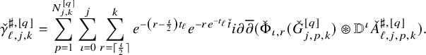 $$ \begin{align} \check{\gamma}^{\sharp,[q]}_{\ell,j,k} = \sum_{p=1}^{N^{[q]}_{j,k}}\sum_{\iota=0}^{j}\sum_{r=\lceil \frac{\iota}{2} \rceil}^{k} e^{-\left(r-\frac{\iota}{2}\right) t_{\ell}}e^{-re^{-t_{\ell}}\check{t}}i\partial\overline\partial(\check{\Phi}_{\iota,r}(\check{G}^{[q]}_{j,p,k})\circledast {\mathbb{D}}^\iota \check{A}^{\sharp,[q]}_{\ell,j,p,k}). \end{align} $$
As in [Reference Hein and Tosatti21, (3.80)], we decompose (3.49) schematically as the sum of
 $6$
pieces
$6$
pieces
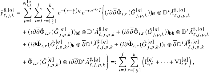 $$ \begin{align}\begin{aligned} \check{\gamma}^{\sharp,[q]}_{\ell,j,k}&= \sum_{p=1}^{N^{[q]}_{j,k}}\sum_{\iota=0}^{j}\sum_{r=\lceil \frac{\iota}{2} \rceil}^{k} e^{-\left(r-\frac{\iota}{2}\right) t_{\ell}}e^{-re^{-t_{\ell}}\check{t}}\bigg\{(i\partial\overline\partial\check{\Phi}_{\iota,r}(\check{G}^{[q]}_{j,p,k}))_{\mathbf{ff}}\circledast {\mathbb{D}}^\iota \check{A}^{\sharp,[q]}_{\ell,j,p,k}\\&\quad+ (i\partial\overline\partial\check{\Phi}_{\iota,r}(\check{G}^{[q]}_{j,p,k}))_{\mathbf{bf}}\circledast {\mathbb{D}}^\iota \check{A}^{\sharp,[q]}_{\ell,j,p,k}+ (i\partial\overline\partial\check{\Phi}_{\iota,r}(\check{G}^{[q]}_{j,p,k}))_{\mathbf{bb}}\circledast {\mathbb{D}}^\iota \check{A}^{\sharp,[q]}_{\ell,j,p,k}\\&\quad+(i\partial\check{\Phi}_{\iota,r}(\check{G}^{[q]}_{j,p,k}))_{\mathbf{b}}\circledast \overline{\partial}{\mathbb{D}}^\iota \check{A}^{\sharp,[q]}_{\ell,j,p,k} +(i\partial\check{\Phi}_{\iota,r}(\check{G}^{[q]}_{j,p,k}))_{\mathbf{f}}\circledast \overline{\partial}{\mathbb{D}}^\iota\check{A}^{\sharp,[q]}_{\ell,j,p,k}\\&\quad+\check{\Phi}_{\iota,r}(\check{G}^{[q]}_{j,p,k})\circledast i\partial\overline{\partial}{\mathbb{D}}^\iota \check{A}^{\sharp,[q]}_{\ell,j,p,k}\bigg\}=:\sum_{\iota=0}^{j}\sum_{r=\lceil \frac{\iota}{2} \rceil}^{k} \left(\mathrm{I}^{[q]}_{\iota,r}+\cdots+\mathrm{VI}^{[q]}_{\iota,r}\right), \end{aligned}\end{align} $$
(which depend on
 $\ell ,j,k$
, but we omit this from the notation for simplicity). Observe here that for all
$\ell ,j,k$
, but we omit this from the notation for simplicity). Observe here that for all
 $(\check {z},\check {y},\check {t})\in \check {Q}_{R\delta _{\ell }^{-1}}$
, we have
$(\check {z},\check {y},\check {t})\in \check {Q}_{R\delta _{\ell }^{-1}}$
, we have
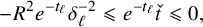 $$ \begin{align} -R^2 e^{-t_{\ell}}\delta_{\ell}^{-2}\leqslant e^{-t_{\ell}}\check{t}\leqslant 0, \end{align} $$
where, by assumption,
 $e^{-t_{\ell }}\delta _{\ell }^{-2}\to 0$
, so the term
$e^{-t_{\ell }}\delta _{\ell }^{-2}\to 0$
, so the term
 $e^{-re^{-t_{\ell }}\check {t}}$
in (3.50) is
$e^{-re^{-t_{\ell }}\check {t}}$
in (3.50) is
 $1+o(1)$
. Now, as in [Reference Hein and Tosatti21, (3.85)–(3.91)], we see that
$1+o(1)$
. Now, as in [Reference Hein and Tosatti21, (3.85)–(3.91)], we see that
 $\mathrm {I}^{[q]}_{0,0}$
is the dominant term, in the sense that
$\mathrm {I}^{[q]}_{0,0}$
is the dominant term, in the sense that
 $$ \begin{align} \|\bullet^{[q]}_{\iota,r}\|_{\infty,\check{Q}_{R\delta_{\ell}^{-1}},\check{g}_{\ell}(0)}\leqslant C\delta_{\ell}\|\mathrm{I}^{[q]}_{0,0}\|_{\infty,\check{Q}_{R\delta_{\ell}^{-1}},\check{g}_{\ell}(0)}, \end{align} $$
whenever
 $\bullet \neq \mathrm {I}$
or
$\bullet \neq \mathrm {I}$
or
 $(\iota ,r)\neq (0,0)$
. This together with (3.11) implies that
$(\iota ,r)\neq (0,0)$
. This together with (3.11) implies that
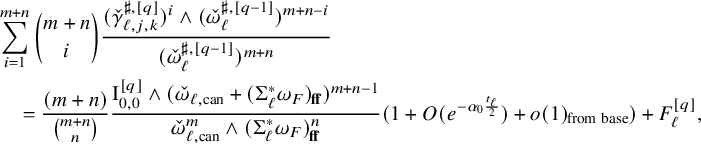 $$ \begin{align}\begin{aligned} &\sum_{i=1}^{m+n}\binom{m+n}{i}\frac{(\check{\gamma}^{\sharp,[q]}_{\ell,j,k})^i\wedge(\check\omega_{\ell}^{\sharp,[q-1]})^{m+n-i}}{(\check\omega_{\ell}^{\sharp,[q-1]})^{m+n}}\\&\quad=\frac{(m+n)}{\binom{m+n}{n}}\frac{\mathrm{I}^{[q]}_{0,0}\wedge(\check{\omega}_{\ell, \mathrm{ can}}+(\Sigma_{\ell}^{*}\omega_F)_{\mathbf{ff}})^{m+n-1}}{\check{\omega}_{\ell, \mathrm{ can}}^m\wedge(\Sigma_{\ell}^{*}\omega_F)^n_{\mathbf{ff}}} (1+O(e^{-\alpha_0\frac{t_{\ell}}{2}})+o(1)_{\mathrm{from\ base}})+F^{[q]}_{\ell}, \end{aligned} \end{align} $$
where given any
 $R>0$
, there is a
$R>0$
, there is a
 $C>0$
such that for all
$C>0$
such that for all
 $\ell $
,
$\ell $
,
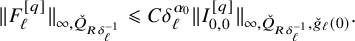 $$ \begin{align} \|F^{[q]}_{\ell}\|_{\infty,\check{Q}_{R\delta_{\ell}^{-1}}}\leqslant C\delta_{\ell}^{\alpha_0}\|I^{[q]}_{0,0}\|_{\infty,\check{Q}_{R\delta_{\ell}^{-1}},\check{g}_{\ell}(0)}. \end{align} $$
Relation (3.2) shows that
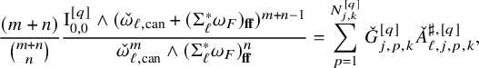 $$ \begin{align} \frac{(m+n)}{\binom{m+n}{n}}\frac{\mathrm{I}^{[q]}_{0,0}\wedge(\check{\omega}_{\ell, \mathrm{ can}}+(\Sigma_{\ell}^{*}\omega_F)_{\mathbf{ff}})^{m+n-1}}{\check{\omega}_{\ell, \mathrm{ can}}^m\wedge(\Sigma_{\ell}^{*}\omega_F)^n_{\mathbf{ff}}}=\sum_{p=1}^{N^{[q]}_{j,k}}\check{G}^{[q]}_{j,p,k}\check{A}^{\sharp,[q]}_{\ell,j,p,k}, \end{align} $$
while from the definition of
 $I^{[q]}_{0,0}$
and (3.8), we have
$I^{[q]}_{0,0}$
and (3.8), we have
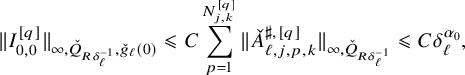 $$ \begin{align} \|I^{[q]}_{0,0}\|_{\infty,\check{Q}_{R\delta_{\ell}^{-1}},\check{g}_{\ell}(0)}\leqslant C \sum_{p=1}^{N^{[q]}_{j,k}}\|\check{A}^{\sharp,[q]}_{\ell,j,p,k}\|_{\infty,\check{Q}_{R\delta_{\ell}^{-1}}}\leqslant C\delta_{\ell}^{\alpha_0}, \end{align} $$
while the argument in [Reference Hein and Tosatti21, (3.83)] gives the reverse bound
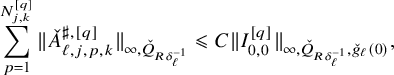 $$ \begin{align} \sum_{p=1}^{N^{[q]}_{j,k}}\|\check{A}^{\sharp,[q]}_{\ell,j,p,k}\|_{\infty,\check{Q}_{R\delta_{\ell}^{-1}}}\leqslant C\|I^{[q]}_{0,0}\|_{\infty,\check{Q}_{R\delta_{\ell}^{-1}},\check{g}_{\ell}(0)}, \end{align} $$
and (3.53), (3.54), (3.55), (3.56) imply in particular that
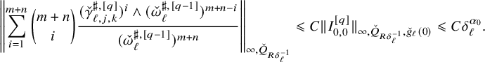 $$ \begin{align} \left\|\sum_{i=1}^{m+n}\binom{m+n}{i}\frac{(\check{\gamma}^{\sharp,[q]}_{\ell,j,k})^i\wedge(\check\omega_{\ell}^{\sharp,[q-1]})^{m+n-i}}{(\check\omega_{\ell}^{\sharp,[q-1]})^{m+n}}\right\|_{\infty,\check{Q}_{R\delta_{\ell}^{-1}}}\leqslant C\|I^{[q]}_{0,0}\|_{\infty,\check{Q}_{R\delta_{\ell}^{-1}},\check{g}_{\ell}(0)}\leqslant C\delta_{\ell}^{\alpha_0}. \end{align} $$
From (3.53), (3.54), (3.55), (3.58) and the Taylor expansion of
 $\log (1+x)$
, we see that
$\log (1+x)$
, we see that
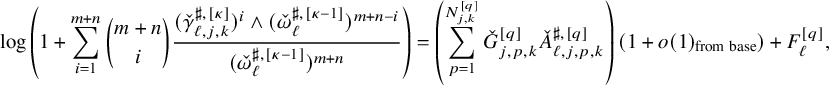 $$ \begin{align} \log\left(1+\sum_{i=1}^{m+n}\binom{m+n}{i}\frac{(\check{\gamma}^{\sharp,[\kappa]}_{\ell,j,k})^i\wedge(\check\omega_{\ell}^{\sharp,[\kappa-1]})^{m+n-i}}{(\check\omega_{\ell}^{\sharp,[\kappa-1]})^{m+n}}\right)= \left(\sum_{p=1}^{N^{[q]}_{j,k}}\check{G}^{[q]}_{j,p,k}\check{A}^{\sharp,[q]}_{\ell,j,p,k}\right)(1+o(1)_{\mathrm{from\ base}})+F^{[q]}_{\ell}, \end{align} $$
where
 $F^{[q]}_{\ell }$
satisfies (3.54).
$F^{[q]}_{\ell }$
satisfies (3.54).
This deals with the term on the second line of (3.47). As for the last line, we can use (3.43) to expand
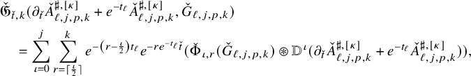 $$ \begin{align} \begin{aligned} &\check{\mathfrak{G}}_{\check{t},k}( \partial_{\check{t}}{\check{A}}^{\sharp,[\kappa]}_{\ell,j,p,k}+e^{-t_{\ell}}\check{A}^{\sharp,[\kappa]}_{\ell,j,p,k},\check G_{\ell,j,p,k})\\& \quad = \sum_{\iota=0}^{j}\sum_{r=\lceil \frac{\iota}{2} \rceil}^{k} e^{-\left(r-\frac{\iota}{2}\right) t_{\ell}}e^{-re^{-t_{\ell}}\check{t}}(\check{\Phi}_{\iota,r}(\check{G}_{\ell,j,p,k})\circledast {\mathbb{D}}^\iota (\partial_{\check{t}}{\check{A}}^{\sharp,[\kappa]}_{\ell,j,p,k}+e^{-t_{\ell}}\check{A}^{\sharp,[\kappa]}_{\ell,j,p,k})), \end{aligned}\end{align} $$
and applying the obvious parabolic extension of [Reference Hein and Tosatti21, Lemma 3.10] to balls of radius
 $R\delta _{\ell }^{-1}$
gives for
$R\delta _{\ell }^{-1}$
gives for
 $\iota \geqslant 0$
,
$\iota \geqslant 0$
,
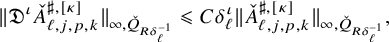 $$ \begin{align} \|\mathfrak{D}^\iota \check{A}^{\sharp,[\kappa]}_{\ell,j,p,k}\|_{\infty,\check{Q}_{R\delta_{\ell}^{-1}}}\leqslant C\delta_{\ell}^{\iota}\| \check{A}^{\sharp,[\kappa]}_{\ell,j,p,k}\|_{\infty,\check{Q}_{R\delta_{\ell}^{-1}}}, \end{align} $$
and so
 $$ \begin{align} \|{\mathbb{D}}^\iota (\partial_{\check{t}}{\check{A}}^{\sharp,[\kappa]}_{\ell,j,p,k}+e^{-t_{\ell}}\check{A}^{\sharp,[\kappa]}_{\ell,j,p,k})\|_{\infty,\check{Q}_{R\delta_{\ell}^{-1}}}\leqslant C\delta_{\ell}^2 \|\mathfrak{D}^\iota \check{A}^{\sharp,[\kappa]}_{\ell,j,p,k}\|_{\infty,\check{Q}_{R\delta_{\ell}^{-1}}}\leqslant C\delta_{\ell}^{\iota+2}\| \check{A}^{\sharp,[\kappa]}_{\ell,j,p,k}\|_{\infty,\check{Q}_{R\delta_{\ell}^{-1}}}. \end{align} $$
Inserting (3.62) into (3.60), and using also (3.57) and the fact that
 $e^{-re^{-t_{\ell }}\check {t}}=1+o(1)$
from (3.51), we see that
$e^{-re^{-t_{\ell }}\check {t}}=1+o(1)$
from (3.51), we see that
 $$ \begin{align} \left\|\check{\mathfrak{G}}_{\check{t},k}( \partial_{\check{t}}{\check{A}}^{\sharp,[\kappa]}_{\ell,j,p,k}+e^{-t_{\ell}}\check{A}^{\sharp,[\kappa]}_{\ell,j,p,k},\check G_{\ell,j,p,k})\right\|_{\infty,\check{Q}_{R\delta_{\ell}^{-1}}}\leqslant C\delta_{\ell}^2 \|I^{[q]}_{0,0}\|_{\infty,\check{Q}_{R\delta_{\ell}^{-1}},\check{g}_{\ell}(0)}, \end{align} $$
and combining this with (3.47) and (3.59), we finally obtain
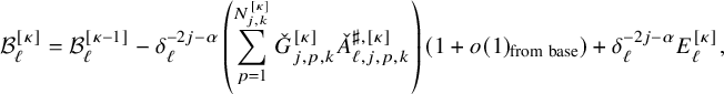 $$ \begin{align} \mathcal{B}_{\ell}^{[\kappa]}=\mathcal{B}_{\ell}^{[\kappa-1]}-\delta_{\ell}^{-2j-\alpha}\left(\sum_{p=1}^{N^{[\kappa]}_{j,k}}\check{G}^{[\kappa]}_{j,p,k}\check{A}^{\sharp,[\kappa]}_{\ell,j,p,k}\right)(1+o(1)_{\mathrm{from\ base}})+\delta_{\ell}^{-2j-\alpha}E^{[\kappa]}_{\ell}, \end{align} $$
where
 $E^{[\kappa ]}_{\ell }$
satisfies
$E^{[\kappa ]}_{\ell }$
satisfies
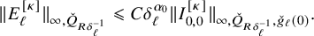 $$ \begin{align} \|E^{[\kappa]}_{\ell}\|_{\infty,\check{Q}_{R\delta_{\ell}^{-1}}}\leqslant C\delta_{\ell}^{\alpha_0}\|I^{[\kappa]}_{0,0}\|_{\infty,\check{Q}_{R\delta_{\ell}^{-1}},\check{g}_{\ell}(0)}. \end{align} $$
Now, from Lemma 3.3, we know that both
 $\mathcal {B}_{\ell }^{[\kappa ]}$
and
$\mathcal {B}_{\ell }^{[\kappa ]}$
and
 $\mathcal {B}_{\ell }^{[\kappa -1]}$
satisfy
$\mathcal {B}_{\ell }^{[\kappa -1]}$
satisfy
 $(\star )$
, and from (3.64), we see that so does
$(\star )$
, and from (3.64), we see that so does
 $\delta _{\ell }^{-2j-\alpha }E^{[\kappa ]}_{\ell }$
, and so it has an expansion of the form (3.25). As in [Reference Hein and Tosatti21], we apply the approximate fiberwise Gram-Schmidt [Reference Hein and Tosatti21, Proposition 3.1] to the functions
$\delta _{\ell }^{-2j-\alpha }E^{[\kappa ]}_{\ell }$
, and so it has an expansion of the form (3.25). As in [Reference Hein and Tosatti21], we apply the approximate fiberwise Gram-Schmidt [Reference Hein and Tosatti21, Proposition 3.1] to the functions
 $h_i$
together with the
$h_i$
together with the
 $G_{i,p,k}, 1\leqslant i<j$
and
$G_{i,p,k}, 1\leqslant i<j$
and
 $G^{[q]}_{j,p,k}, 1\leqslant q\leqslant \kappa $
; this produces our desired list
$G^{[q]}_{j,p,k}, 1\leqslant q\leqslant \kappa $
; this produces our desired list
 $G^{[\kappa +1]}_{j,p,k}$
(on
$G^{[\kappa +1]}_{j,p,k}$
(on
 $B_r\times Y$
, up to shrinking r), so that we may assume that the functions
$B_r\times Y$
, up to shrinking r), so that we may assume that the functions
 $h_i$
in (3.25) lie in the fiberwise linear span of the
$h_i$
in (3.25) lie in the fiberwise linear span of the
 $G_{i,p,k}, 1\leqslant i<j$
together with the
$G_{i,p,k}, 1\leqslant i<j$
together with the
 $G^{[q]}_{j,p,k}, 1\leqslant q\leqslant \kappa +1$
. This completes the step from
$G^{[q]}_{j,p,k}, 1\leqslant q\leqslant \kappa +1$
. This completes the step from
 $\kappa $
to
$\kappa $
to
 $\kappa +1$
in our iterative procedure.
$\kappa +1$
in our iterative procedure.
Iterating (3.64) shows that for every
 $\kappa \geqslant 1$
, we have
$\kappa \geqslant 1$
, we have
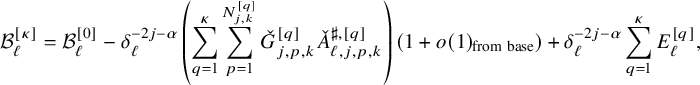 $$ \begin{align} \mathcal{B}_{\ell}^{[\kappa]}=\mathcal{B}_{\ell}^{[0]}-\delta_{\ell}^{-2j-\alpha}\left(\sum_{q=1}^\kappa\sum_{p=1}^{N^{[q]}_{j,k}}\check{G}^{[q]}_{j,p,k}\check{A}^{\sharp,[q]}_{\ell,j,p,k}\right) (1+o(1)_{\mathrm{from\ base}})+\delta_{\ell}^{-2j-\alpha}\sum_{q=1}^\kappa E^{[q]}_{\ell}, \end{align} $$
with
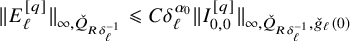 $$ \begin{align} \|E^{[q]}_{\ell}\|_{\infty,\check{Q}_{R\delta_{\ell}^{-1}}}\leqslant C\delta_{\ell}^{\alpha_0}\|I^{[q]}_{0,0}\|_{\infty,\check{Q}_{R\delta_{\ell}^{-1}},\check{g}_{\ell}(0)} \end{align} $$
for
 $1\leqslant q\leqslant \kappa $
, and also
$1\leqslant q\leqslant \kappa $
, and also
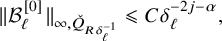 $$ \begin{align} \|\mathcal{B}_{\ell}^{[0]}\|_{\infty,\check{Q}_{R\delta_{\ell}^{-1}}}\leqslant C\delta_{\ell}^{-2j-\alpha}, \end{align} $$
which follows immediately from (3.29).
We can now repeat the iterative step
 $\overline {\kappa }:=\lceil \frac {2j+\alpha }{\alpha _0}\rceil $
and then we stop, so the last set of functions which are added to the list are the
$\overline {\kappa }:=\lceil \frac {2j+\alpha }{\alpha _0}\rceil $
and then we stop, so the last set of functions which are added to the list are the
 $G_{j,p,k}^{[\overline {\kappa }+1]}$
. Our choice of
$G_{j,p,k}^{[\overline {\kappa }+1]}$
. Our choice of
 $\overline {\kappa }$
is made so that
$\overline {\kappa }$
is made so that
 $$ \begin{align} \delta_{\ell}^{-2j-\alpha}\delta_{\ell}^{(\overline{\kappa}+1)\alpha_0}\to 0. \end{align} $$
The resulting
 $G_{j,p,k}^{[q]}$
with
$G_{j,p,k}^{[q]}$
with
 $1\leqslant q\leqslant \overline {\kappa }+1$
are then renamed simply
$1\leqslant q\leqslant \overline {\kappa }+1$
are then renamed simply
 $G_{j,p,k}$
. These, together with the
$G_{j,p,k}$
. These, together with the
 $G_{i,p,k}, 1\leqslant i<j$
, are the obstruction functions that we seek. It remains to show that the statement of the Selection Theorem 3.1 holds with this choice of obstruction functions. By definition, the quantity in (3.15) equals
$G_{i,p,k}, 1\leqslant i<j$
, are the obstruction functions that we seek. It remains to show that the statement of the Selection Theorem 3.1 holds with this choice of obstruction functions. By definition, the quantity in (3.15) equals
 $\mathcal {B}_{\ell }^{[\overline {\kappa }+1]}$
(up to the term with
$\mathcal {B}_{\ell }^{[\overline {\kappa }+1]}$
(up to the term with
 $\Sigma _{\ell }^{*}B^\sharp _{\ell }$
, which we can ignore since it can be absorbed into
$\Sigma _{\ell }^{*}B^\sharp _{\ell }$
, which we can ignore since it can be absorbed into
 $f_{\ell ,0}$
in (3.19)). We know that
$f_{\ell ,0}$
in (3.19)). We know that
 $\mathcal {B}_{\ell }^{[\overline {\kappa }+1]}$
satisfies
$\mathcal {B}_{\ell }^{[\overline {\kappa }+1]}$
satisfies
 $(\star )$
thanks to Lemma 3.3. As mentioned earlier, because of this we know that if it converges locally uniformly, then it converges locally smoothly, which is the last claim in the Selection Theorem 3.1. The last thing to prove is that if
$(\star )$
thanks to Lemma 3.3. As mentioned earlier, because of this we know that if it converges locally uniformly, then it converges locally smoothly, which is the last claim in the Selection Theorem 3.1. The last thing to prove is that if
 $\mathcal {B}_{\ell }^{[\overline {\kappa }+1]}$
converges locally uniformly, then (3.19) holds, and thanks to (3.66) (with
$\mathcal {B}_{\ell }^{[\overline {\kappa }+1]}$
converges locally uniformly, then (3.19) holds, and thanks to (3.66) (with
 $\kappa =\overline {\kappa }+1$
) and to our choice of obstruction functions, it suffices to show that
$\kappa =\overline {\kappa }+1$
) and to our choice of obstruction functions, it suffices to show that
 $\delta _{\ell }^{-2j-\alpha }E^{[\overline {\kappa }+1]}_{\ell }$
is
$\delta _{\ell }^{-2j-\alpha }E^{[\overline {\kappa }+1]}_{\ell }$
is
 $o(1)$
in the locally smooth topology. Since this term satisfies
$o(1)$
in the locally smooth topology. Since this term satisfies
 $(\star )$
(as mentioned earlier), it suffices to show that it is
$(\star )$
(as mentioned earlier), it suffices to show that it is
 $o(1)$
in the
$o(1)$
in the
 $L^\infty _{\mathrm {loc}}$
topology, and this follows from (3.66), (3.67), (3.68), (3.69) and our main assumption that
$L^\infty _{\mathrm {loc}}$
topology, and this follows from (3.66), (3.67), (3.68), (3.69) and our main assumption that
 $\mathcal {B}_{\ell }^{[\overline {\kappa }+1]}=O(1)$
in
$\mathcal {B}_{\ell }^{[\overline {\kappa }+1]}=O(1)$
in
 $L^\infty _{\mathrm {loc}}$
, by using the same iteration argument as [Reference Hein and Tosatti21, (3.101)–(3.112)]. This completes the proof of Theorem 3.1.
$L^\infty _{\mathrm {loc}}$
, by using the same iteration argument as [Reference Hein and Tosatti21, (3.101)–(3.112)]. This completes the proof of Theorem 3.1.
4 Asymptotic expansion
In this section, we will prove our main technical result, Theorem 4.2, which gives an asymptotic expansion for the metrics
 $\omega ^{\bullet }(t)$
which evolve under the Kähler-Ricci flow (1.1). Recall that
$\omega ^{\bullet }(t)$
which evolve under the Kähler-Ricci flow (1.1). Recall that
 $\omega ^{\bullet }(t)=\omega ^\natural (t)+{i\partial \bar \partial }\varphi (t)$
, where the potentials
$\omega ^{\bullet }(t)=\omega ^\natural (t)+{i\partial \bar \partial }\varphi (t)$
, where the potentials
 $\varphi (t)$
solve the parabolic complex Monge-Ampère equation (1.6), which we can write as
$\varphi (t)$
solve the parabolic complex Monge-Ampère equation (1.6), which we can write as
 $$ \begin{align} (\omega^{\bullet}(t))^{m+n}=(\omega^\natural(t)+{i\partial\bar\partial}\varphi (t))^{m+n}=e^{\varphi (t)+\dot{\varphi }(t)-nt}\binom{m+n}{n}\omega_{\mathrm{can}}^m\wedge\omega_F^n. \end{align} $$
4.1 Known estimates
First, let us recall a few of the known estimates for the Kähler-Ricci flow (1.1) and its equivalent formulation (1.6). There are many other facts that are known about this flow (see, for example, [Reference Tosatti39, §5] or [Reference Tosatti42, §7] for overviews), but the following are the only ones that we will need:
Lemma 4.1. Assume the setup in Section 1.2. Then there exists
 $C>0$
such that on
$C>0$
such that on
 $B\times Y\times [0,+\infty )$
, we have
$B\times Y\times [0,+\infty )$
, we have
-
(i)
$C^{-1}\omega ^\natural (t)\leqslant \omega ^{\bullet }(t)\leqslant C\omega ^\natural (t)$
, -
(ii)
$|\varphi (t)|+|\dot \varphi (t)|\to 0$
as
$t\to +\infty $
, -
(iii)
$|\omega ^{\bullet }(t)- \omega _{\mathrm {can}}|_{g^{\bullet }(t)}\to 0$
as
$t\to +\infty ,$
-
(iv)
$|R({g^{\bullet }(t)})|\leqslant C$
, -
(v)
$|\dot {\varphi }(t)+\ddot {\varphi }(t)|\leqslant C$
, -
(vi)
$|\nabla (\varphi (t)+\dot {\varphi }(t))|_{g^{\bullet }(t)}\leqslant C.$


Proof. Item (i) is proved in [Reference Fong and Zhang12] (and is an adaptation of [Reference Tosatti38]; see also [Reference Song and Tian31] for the case
 $m=n=1$
). Item (ii) is proved in [Reference Tosatti, Weinkove and Yang43, Lemma 3.1], and item (iii) in [Reference Tosatti, Weinkove and Yang43, Theorem 1.2] (see especially the very end of its proof on p.685). Item (iv) is the main theorem of [Reference Song and Tian33], and this implies (v) thanks to the relation [Reference Tosatti39, p.345]
$m=n=1$
). Item (ii) is proved in [Reference Tosatti, Weinkove and Yang43, Lemma 3.1], and item (iii) in [Reference Tosatti, Weinkove and Yang43, Theorem 1.2] (see especially the very end of its proof on p.685). Item (iv) is the main theorem of [Reference Song and Tian33], and this implies (v) thanks to the relation [Reference Tosatti39, p.345]
 $$ \begin{align} \dot{\varphi }(t)+\ddot{\varphi }(t)=-R(g^{\bullet}(t))-m. \end{align} $$
To prove (vi), we use [Reference Song and Tian33, Proposition 3.1] which gives
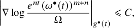 $$ \begin{align} \left|\nabla\log \frac{e^{nt}(\omega^{\bullet}(t))^{m+n}}{\Omega}\right|_{g^{\bullet}(t)}\leqslant C, \end{align} $$
where
 $\Omega $
is a smooth positive volume form on X such that
$\Omega $
is a smooth positive volume form on X such that
 $-{i\partial \bar \partial }\log \Omega =-\omega _B$
is the pullback of a Kähler form on B. However, by [Reference Tosatti39, Proposition 5.9], we have
$-{i\partial \bar \partial }\log \Omega =-\omega _B$
is the pullback of a Kähler form on B. However, by [Reference Tosatti39, Proposition 5.9], we have
 $-{i\partial \bar \partial }\log (\omega _{\mathrm { can}}^m\wedge \omega _F^n)=-\omega _{\mathrm {can}},$
so on
$-{i\partial \bar \partial }\log (\omega _{\mathrm { can}}^m\wedge \omega _F^n)=-\omega _{\mathrm {can}},$
so on
 $B\times Y$
, we have
$B\times Y$
, we have
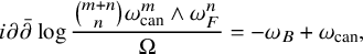 $$ \begin{align} {i\partial\bar\partial}\log \frac{\binom{m+n}{n}\omega_{\mathrm{can}}^m\wedge\omega_F^n}{\Omega}=-\omega_B+\omega_{\mathrm{can}}, \end{align} $$
which is a
 $(1,1)$
-form pulled back from B; hence, the logarithm of the ratio of these two volume forms restricted to the fibers
$(1,1)$
-form pulled back from B; hence, the logarithm of the ratio of these two volume forms restricted to the fibers
 $\{z\}\times Y$
is pluriharmonic, hence constant. Thus,
$\{z\}\times Y$
is pluriharmonic, hence constant. Thus,
 $$ \begin{align} \binom{m+n}{n}\omega_{\mathrm{can}}^m\wedge\omega_F^n=e^G\Omega \end{align} $$
for some smooth function G on B, and so using (4.1) and (4.3), we get
 $$ \begin{align} |\nabla(\varphi (t)+\dot{\varphi }(t))|_{g^{\bullet}(t)}=\left|\nabla\left(\log \frac{e^{nt}(\omega^{\bullet}(t))^{m+n}}{\Omega}-G\right) \right|_{g^{\bullet}(t)}\leqslant C+|\nabla G|_{g^{\bullet}(t)}\leqslant C, \end{align} $$
as desired.
4.2 Statement of the asymptotic expansion
Given any
 $j\in \mathbb {N}, 0\leqslant 2j\leqslant k$
and
$j\in \mathbb {N}, 0\leqslant 2j\leqslant k$
and
 $z\in B$
, during the course of the proof of Theorem 4.2 below, we will work by induction on j. By applying repeatedly the Selection Theorem 3.1, and consequently shrinking our ball at each step, we will obtain in particular a collection
$z\in B$
, during the course of the proof of Theorem 4.2 below, we will work by induction on j. By applying repeatedly the Selection Theorem 3.1, and consequently shrinking our ball at each step, we will obtain in particular a collection
 $G_{i,p,k}, 1\leqslant i\leqslant j, 1\leqslant p\leqslant N_{i,k}$
of smooth function on
$G_{i,p,k}, 1\leqslant i\leqslant j, 1\leqslant p\leqslant N_{i,k}$
of smooth function on
 $B\times Y$
with fiberwise average zero, which are fiberwise
$B\times Y$
with fiberwise average zero, which are fiberwise
 $L^2$
orthonormal. For each such
$L^2$
orthonormal. For each such
 $G_{i,p,k}$
and
$G_{i,p,k}$
and
 $t>0$
, as in [Reference Hein and Tosatti21, (3.6)], we define
$t>0$
, as in [Reference Hein and Tosatti21, (3.6)], we define
 $P_{t,i,p,k}=P_{t,G_{i,p,k}}$
, where
$P_{t,i,p,k}=P_{t,G_{i,p,k}}$
, where
 $$ \begin{align} P_{t,H}({\alpha})= n(\mathrm{pr}_{B})_* (H {\alpha} \wedge \omega_F^{n-1})+e^{-t} \operatorname{tr}_{\omega_{\mathrm{can}}}(\mathrm{pr}_{B})_*(H {\alpha} \wedge \omega_F^n), \end{align} $$
for any
 $(1,1)$
form
$(1,1)$
form
 ${\alpha }$
on
${\alpha }$
on
 $B\times Y$
and H with
$B\times Y$
and H with
 $\int _{\{z\}\times Y}H\omega _F^n=0$
for all
$\int _{\{z\}\times Y}H\omega _F^n=0$
for all
 $z\in \mathbb {C}^m$
. Throughout the proof, we will fix a reference shrinking product metric
$z\in \mathbb {C}^m$
. Throughout the proof, we will fix a reference shrinking product metric
 $g(t)=g_{\mathbb {C}^m}+e^{-t} g_{Y,z_0}$
. It will only be used to measure the norms and distance but not the connection, and thus the exact choice of
$g(t)=g_{\mathbb {C}^m}+e^{-t} g_{Y,z_0}$
. It will only be used to measure the norms and distance but not the connection, and thus the exact choice of
 $z_0$
is unimportant thanks to (2.5) (we will usually take
$z_0$
is unimportant thanks to (2.5) (we will usually take
 $z_0=0$
). We will also need the t-dependent approximate Green operator
$z_0=0$
). We will also need the t-dependent approximate Green operator
 $\mathfrak {G}_{t,k}$
defined in [Reference Hein and Tosatti21, §3.2], to which we refer for its basic properties.
$\mathfrak {G}_{t,k}$
defined in [Reference Hein and Tosatti21, §3.2], to which we refer for its basic properties.
Theorem 4.2. For all
 $j,k\in \mathbb {N},0\leqslant 2j\leqslant k$
,
$j,k\in \mathbb {N},0\leqslant 2j\leqslant k$
,
 $z\in B$
, there exists
$z\in B$
, there exists
 $B'=B_{\mathbb {C}^m}(z,R)\Subset B$
and functions
$B'=B_{\mathbb {C}^m}(z,R)\Subset B$
and functions
 $G_{i,p,k}, 1\leqslant i\leqslant j, 1\leqslant p\leqslant N_{i,k}$
as above, such that on
$G_{i,p,k}, 1\leqslant i\leqslant j, 1\leqslant p\leqslant N_{i,k}$
as above, such that on
 $B'\times Y$
, we have a decomposition
$B'\times Y$
, we have a decomposition
 $$ \begin{align} \omega^{\bullet}(t)=\omega^\natural(t)+\gamma_0(t)+\gamma_{1,k}(t)+\dots+\gamma_{j,k}(t)+\eta_{j,k}(t), \end{align} $$
with the following properties. For all
 ${\alpha }\in (0,1)$
and
${\alpha }\in (0,1)$
and
 $r<R$
, there is
$r<R$
, there is
 $C>0$
such that for all
$C>0$
such that for all
 $t\geqslant 0$
,
$t\geqslant 0$
,
 $$ \begin{align} \|\mathfrak{D}^\iota \eta_{j,k}\|_{\infty,Q_r(z,t),g(t)} \leqslant Ce^{\frac{\iota-2j-{\alpha}}{2}t}\,\;\;\text{for all}\;\; 0\leqslant \iota\leqslant 2j, \end{align} $$
 $$ \begin{align} [\mathfrak{D}^{2j}\eta_{j,k}]_{{\alpha},{\alpha}/2, Q_r(z,t),g(t)}\leqslant C, \end{align} $$
where
 $Q_r(z,t)=\left(B_{\mathbb {C}^m}(z,r)\times Y\right)\times [t-r^2,t]$
. Furthermore, we have
$Q_r(z,t)=\left(B_{\mathbb {C}^m}(z,r)\times Y\right)\times [t-r^2,t]$
. Furthermore, we have
 $$ \begin{align} \gamma_0(t)={i\partial\bar\partial} \underline{\varphi},\;\;\; \gamma_{i,k}(t)=\sum_{p=1}^{N_{i,k}}{i\partial\bar\partial} \mathfrak{G}_{t,k}\left(A_{i,p,k}(t),G_{i,p,k} \right), \end{align} $$
for
 $1\leqslant i\leqslant j$
where
$1\leqslant i\leqslant j$
where
 $A_{i,p,k}(t)=P_{t,i,p,k}(\eta _{i-1,k}(t))$
are functions from the base, and we have
$A_{i,p,k}(t)=P_{t,i,p,k}(\eta _{i-1,k}(t))$
are functions from the base, and we have
 $$ \begin{align} \|\mathfrak{D}^\iota\gamma_{0}\|_{\infty, Q_r(z,t),g_{\mathbb{C}^m}} = o(1)\,\;\;\text{for all}\;\; 0\leqslant \iota\leqslant 2j, \end{align} $$
 $$ \begin{align} \quad [\mathfrak{D}^{2j}\gamma_{0}]_{{\alpha},{\alpha}/2, Q_r(z,t),g_{\mathbb{C}^m}} \leqslant C, \end{align} $$
 $$ \begin{align} \|\mathfrak{D}^\iota(\partial_t\underline{\varphi }+\underline{\varphi })\|_{\infty, Q_r(z,t),g_{\mathbb{C}^m}} = o(1)\,\;\;\text{for all}\;\; 0\leqslant \iota\leqslant 2j, \end{align} $$
 $$ \begin{align} \quad [\mathfrak{D}^{2j}(\partial_t\underline{\varphi }+\underline{\varphi })]_{{\alpha},{\alpha}/2, Q_r(z,t),g_{\mathbb{C}^m}} \leqslant C, \end{align} $$
 $$ \begin{align} \|\mathfrak{D}^\iota A_{i,p,k}\|_{\infty,Q_r(z,t),g_{\mathbb{C}^m}}\leqslant Ce^{-(2i+{\alpha})(1-\frac{\iota}{2j+2+{\alpha}})\frac{t}2},\;\;\text{for all} \;\; 0\leqslant \iota\leqslant 2j+2,1\leqslant i \leqslant j,1\leqslant p\leqslant N_{i,k}, \end{align} $$
 $$ \begin{align} \|\mathfrak{D}^{2j+2+\iota} A_{i,p,k}\|_{\infty,Q_r(z,t),g_{\mathbb{C}^m}}\leqslant Ce^{\left(-\frac{{\alpha}(2i+{\alpha})}{\iota+{\alpha}}(1-\frac{2j+2}{2j+2+{\alpha}})+\frac{\iota^2}{\iota+{\alpha}}\right) \frac{t}{2}},\,\;\;\text{for all}\;\; 0\leqslant \iota\leqslant 2k,\;\, 1\leqslant i \leqslant j,\;\,1\leqslant p\leqslant N_{i,k}, \end{align} $$
 $$ \begin{align} \begin{aligned} \sup_{(x,s),(x',s')\in Q_r(z,t)}\sum_{i=1}^{j} \sum_{p=1}^{N_{i,k}}\sum_{\iota = -2}^{2k} &e^{-\iota\frac{t}{2}}\Bigg(\frac{|\mathfrak{D}^{2j+2+\iota} A_{i,p,k}(x,s)-\mathbb{P}_{x'x}(\mathfrak{D}^{2j+2+\iota}A_{i,p,k}(x',s'))|_{g(t)}}{ \left( d^{g(t)}(x,x') +|s-s'|^{\frac{1}{2}} \right)^{\alpha}}\Bigg)\leqslant C. \end{aligned} \end{align} $$
Remark 4.3. Key differences between Theorem 4.2 and [Reference Hein and Tosatti21, Theorem 4.1] are the estimates in (4.14), (4.15). These will be crucial for us in the proof, to deal with the term
 $\partial _t\varphi +\varphi $
in the complex Monge-Ampère equation (4.1). Another difference is that the bounds in (4.16) are worse than those in [Reference Hein and Tosatti21, (4.12)], due to the fact that in this paper, we can only consider even order Hölder norms.
$\partial _t\varphi +\varphi $
in the complex Monge-Ampère equation (4.1). Another difference is that the bounds in (4.16) are worse than those in [Reference Hein and Tosatti21, (4.12)], due to the fact that in this paper, we can only consider even order Hölder norms.
4.3 Setup of induction scheme
We start with a given
 $z\in B$
. For any given
$z\in B$
. For any given
 $k\in \mathbb {N}$
, we prove the Theorem by induction on j. We treat both the base case and induction case together, although they will have to be considered separately at certain steps of the proof. Given k with
$k\in \mathbb {N}$
, we prove the Theorem by induction on j. We treat both the base case and induction case together, although they will have to be considered separately at certain steps of the proof. Given k with
 $0\leqslant 2j\leqslant k$
, if
$0\leqslant 2j\leqslant k$
, if
 $j>0$
, we assume Theorem 4.2 holds at the
$j>0$
, we assume Theorem 4.2 holds at the
 $(j-1)$
-th step, so there exists
$(j-1)$
-th step, so there exists
 $B_{\mathbb {C}^m}(z,r)\subset B$
such that we already have the decomposition of
$B_{\mathbb {C}^m}(z,r)\subset B$
such that we already have the decomposition of
 $\omega ^{\bullet }(t)$
at the
$\omega ^{\bullet }(t)$
at the
 $(j-1)$
-th step satisfying the desired estimates on
$(j-1)$
-th step satisfying the desired estimates on
 $B_{\mathbb {C}^m}(z,r)\times Y\times [0,+\infty )$
. We aim to refine the decomposition at the j-th step as well as define it for
$B_{\mathbb {C}^m}(z,r)\times Y\times [0,+\infty )$
. We aim to refine the decomposition at the j-th step as well as define it for
 $j=0$
.
$j=0$
.
As mentioned in the Introduction, we can write
 $\omega ^{\bullet }=\omega ^\natural +{i\partial \bar \partial } \varphi $
. When
$\omega ^{\bullet }=\omega ^\natural +{i\partial \bar \partial } \varphi $
. When
 $j=0$
, we take
$j=0$
, we take
 $\gamma _0={i\partial \bar \partial }\underline{\varphi }$
and
$\gamma _0={i\partial \bar \partial }\underline{\varphi }$
and
 $\eta _{0,k}={i\partial \bar \partial } (\varphi -\underline{\varphi })$
so that
$\eta _{0,k}={i\partial \bar \partial } (\varphi -\underline{\varphi })$
so that
 $\omega ^{\bullet }=\omega ^\natural +\gamma _0+\eta _{0,k}$
. If
$\omega ^{\bullet }=\omega ^\natural +\gamma _0+\eta _{0,k}$
. If
 $j\geqslant 1$
, suppose we already have the decomposition
$j\geqslant 1$
, suppose we already have the decomposition
 $$ \begin{align} \omega^{\bullet}=\omega^\natural+\gamma_0+\gamma_{1,k}+\dots+\gamma_{j-1,k}+\eta_{j-1,k} \end{align} $$
on
 $\left(B_{\mathbb {C}^m}(z,r)\times Y\right)\times [0,+\infty )$
. We further decompose
$\left(B_{\mathbb {C}^m}(z,r)\times Y\right)\times [0,+\infty )$
. We further decompose
 $\eta _{j-1,k}$
into
$\eta _{j-1,k}$
into
 $\gamma _{j,k}+\eta _{j,k}$
as follows. When
$\gamma _{j,k}+\eta _{j,k}$
as follows. When
 $j>1$
, up to shrinking
$j>1$
, up to shrinking
 $r>0$
, we can assume that we already have selected smooth functions
$r>0$
, we can assume that we already have selected smooth functions
 $G_{i,p,k},1\leqslant i\leqslant j-1, 1\leqslant p\leqslant N_{i,k}$
on
$G_{i,p,k},1\leqslant i\leqslant j-1, 1\leqslant p\leqslant N_{i,k}$
on
 $B_{\mathbb {C}^m}(z,r)\times Y$
, which are fiberwise
$B_{\mathbb {C}^m}(z,r)\times Y$
, which are fiberwise
 $L^2$
orthonormal and have fiberwise average zero. When
$L^2$
orthonormal and have fiberwise average zero. When
 $j\geqslant 1$
, we then apply the Selection Theorem 3.1 which up to shrinking r further, gives us a list of functions
$j\geqslant 1$
, we then apply the Selection Theorem 3.1 which up to shrinking r further, gives us a list of functions
 $G_{j,p,k}, 1\leqslant p\leqslant N_{j,k}$
on
$G_{j,p,k}, 1\leqslant p\leqslant N_{j,k}$
on
 $B_{\mathbb {C}^m}(z,r)\times Y$
, which are fiberwise
$B_{\mathbb {C}^m}(z,r)\times Y$
, which are fiberwise
 $L^2$
orthonormal and have fiberwise average zero, so that the conclusion of the Selection Theorem 3.1 holds for the collection
$L^2$
orthonormal and have fiberwise average zero, so that the conclusion of the Selection Theorem 3.1 holds for the collection
 $G_{i,p,k}, 1\leqslant p\leqslant N_{i,k},1\leqslant i\leqslant j$
. With this collection of function, we define
$G_{i,p,k}, 1\leqslant p\leqslant N_{i,k},1\leqslant i\leqslant j$
. With this collection of function, we define
 $$ \begin{align} A_{j,p,k}(t):=P_{t,j,p,k}(\eta_{j-1,k}(t)), \end{align} $$
where P is given by (4.7) and
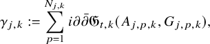 $$ \begin{align} \gamma_{j,k}:=\sum_{p=1}^{N_{j,k}}{i\partial\bar\partial} \mathfrak{G}_{t,k}(A_{j,p,k},G_{j,p,k}), \end{align} $$
where
 $\mathfrak {G}_{t,k}$
is defined in [Reference Hein and Tosatti21, §3.2]. Finally, we define
$\mathfrak {G}_{t,k}$
is defined in [Reference Hein and Tosatti21, §3.2]. Finally, we define
 $\eta _{j,k}:=\eta _{j-1,k}-\gamma _{j,k}$
so that
$\eta _{j,k}:=\eta _{j-1,k}-\gamma _{j,k}$
so that
 $$ \begin{align} \omega^{\bullet}=\omega^\natural+\gamma_0+\gamma_{1,k}+\dots+\gamma_{j,k}+\eta_{j,k} \end{align} $$
on
 $B_{\mathbb {C}^m}(z,r)\times Y\times [0,+\infty )$
. For ease of notation, by scaling and translation of our coordinates, we may assume without loss that we have this decomposition
$B_{\mathbb {C}^m}(z,r)\times Y\times [0,+\infty )$
. For ease of notation, by scaling and translation of our coordinates, we may assume without loss that we have this decomposition
 $B_{\mathbb {C}^m}(z,r)=B_{\mathbb {C}^m}(1)=B$
.
$B_{\mathbb {C}^m}(z,r)=B_{\mathbb {C}^m}(1)=B$
.
4.3.1 The base case of the induction
$j=0$

The base case of the induction, where
 $j=0$
, needs to be treated separately, and although the overall scheme of proof is the same as when
$j=0$
, needs to be treated separately, and although the overall scheme of proof is the same as when
 $j\geqslant 1$
, there will be some crucial differences.
$j\geqslant 1$
, there will be some crucial differences.
First of all, let us examine the estimates that we need to prove in order to establish Theorem 4.2 for
 $j=0$
. The estimates (4.16), (4.17), (4.18) are vacuous by definition. By Lemma 4.1 (iii), we have that
$j=0$
. The estimates (4.16), (4.17), (4.18) are vacuous by definition. By Lemma 4.1 (iii), we have that
 $\|{i\partial \bar \partial }\varphi \|_{\infty , B\times Y\times [t-1,t],g(t)}=o(1)$
as
$\|{i\partial \bar \partial }\varphi \|_{\infty , B\times Y\times [t-1,t],g(t)}=o(1)$
as
 $t\to +\infty $
, and the fiber integration argument in [Reference Tosatti38, p. 436] then gives
$t\to +\infty $
, and the fiber integration argument in [Reference Tosatti38, p. 436] then gives
 $\|\gamma _0\|_{\infty , B\times [t-1,t],g_{\mathbb {C}^m}}=o(1)$
as well, which implies (4.12). Similarly, Lemma 4.1 (ii) implies that
$\|\gamma _0\|_{\infty , B\times [t-1,t],g_{\mathbb {C}^m}}=o(1)$
as well, which implies (4.12). Similarly, Lemma 4.1 (ii) implies that
 $\|\partial _t\varphi +\varphi \|_{\infty , B\times Y\times [t-1,t]}=o(1)$
, and taking fiberwise average, this easily implies that
$\|\partial _t\varphi +\varphi \|_{\infty , B\times Y\times [t-1,t]}=o(1)$
, and taking fiberwise average, this easily implies that
 $\|\partial _t\underline{\varphi }+\underline{\varphi }\|_{\infty , B\times [t-1,t]}=o(1)$
too, which implies (4.14).
$\|\partial _t\underline{\varphi }+\underline{\varphi }\|_{\infty , B\times [t-1,t]}=o(1)$
too, which implies (4.14).
Next, using the bounds
 $\|\partial _{t}^2\varphi +\partial _{t}\varphi \|_{\infty , B\times Y\times [t-1,t]}\leqslant C$
and
$\|\partial _{t}^2\varphi +\partial _{t}\varphi \|_{\infty , B\times Y\times [t-1,t]}\leqslant C$
and
 $\|\nabla (\partial _{t}\varphi +\varphi )\|_{\infty , B\times Y\times [t-1,t], g(t)}\leqslant C$
from Lemma 4.1 (v), (vi), which together with the
$\|\nabla (\partial _{t}\varphi +\varphi )\|_{\infty , B\times Y\times [t-1,t], g(t)}\leqslant C$
from Lemma 4.1 (v), (vi), which together with the
 $L^\infty $
bound for
$L^\infty $
bound for
 $\partial _t\varphi +\varphi $
imply the same bounds for the fiber average
$\partial _t\varphi +\varphi $
imply the same bounds for the fiber average
 $$ \begin{align} \|\partial_{t}^2\underline{\varphi }+\partial_{t}\underline{\varphi }\|_{\infty, B\times [t-1,t]}\leqslant C,\quad \|\nabla(\partial_{t}\underline{\varphi }+\underline{\varphi })\|_{\infty, B\times [t-1,t],g_{\mathbb{C}^m}}\leqslant C, \end{align} $$
we can bound for any
 $x,x'\in B$
and
$x,x'\in B$
and
 $t\geqslant 0$
and
$t\geqslant 0$
and
 $s\in [t-1,t]$
,
$s\in [t-1,t]$
,
 $$ \begin{align} |(\partial_{t}\underline{\varphi }+\underline{\varphi })(x,t)-(\partial_{t}\underline{\varphi }+\underline{\varphi })(x',s)|\leqslant C(|x-x'|+|t-s|)\leqslant C(|x-x'|+|t-s|^{\frac{1}{2}})^{\alpha}, \end{align} $$
which gives
 $$ \begin{align} [\partial_{t}\underline{\varphi }+\underline{\varphi }]_{{\alpha},{\alpha}/2,B\times [t-1,t],g_{\mathbb{C}^m}}\leqslant C, \end{align} $$
which implies (4.15).
Thus, when
 $j=0$
, it suffices to establish (4.9), (4.10) and (4.13). The final claim we will need is that if we suppose we have proved that for all
$j=0$
, it suffices to establish (4.9), (4.10) and (4.13). The final claim we will need is that if we suppose we have proved that for all
 $t\geqslant 0$
we have
$t\geqslant 0$
we have
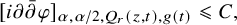 $$ \begin{align} [{i\partial\bar\partial}\varphi ]_{{\alpha},{\alpha}/2, Q_r(z,t),g(t)}\leqslant C, \end{align} $$
where
 $Q_r(z,t)$
is as in the statement of Theorem 4.2, then the estimates (4.9), (4.10) and (4.13) will all hold. To prove this claim, we use the following ‘non-cancellation’ inequality
$Q_r(z,t)$
is as in the statement of Theorem 4.2, then the estimates (4.9), (4.10) and (4.13) will all hold. To prove this claim, we use the following ‘non-cancellation’ inequality
 $$ \begin{align} [{i\partial\bar\partial}\underline{\varphi }]_{{\alpha},{\alpha}/2,B_{\mathbb{C}^m}(z,r)\times[t-r^2,t],g_{\mathbb{C}^m}}\leqslant C[{i\partial\bar\partial}\varphi ]_{{\alpha},{\alpha}/2, \textrm{base}, Q_r(z,t),g_X}+C\|{i\partial\bar\partial}\varphi \|_{\infty, Q_r(z,t),g_X}, \end{align} $$
which is straightforward to prove using [Reference Hein and Tosatti21, (4.215)], except that here there is no stretching involved. Plugging (4.26) and Lemma 4.1 (iii) into (4.27) gives
 $$ \begin{align} [{i\partial\bar\partial}\underline{\varphi }]_{{\alpha},{\alpha}/2,B_{\mathbb{C}^m}(z,r)\times[t-r^2,t],g_{\mathbb{C}^m}}\leqslant C, \end{align} $$
which is exactly (4.13), and recalling that
 $\eta _{0,k}={i\partial \bar \partial }\varphi -{i\partial \bar \partial }\underline{\varphi }$
, we can use (4.26), (4.28), the triangle inequality and the boundedness of
$\eta _{0,k}={i\partial \bar \partial }\varphi -{i\partial \bar \partial }\underline{\varphi }$
, we can use (4.26), (4.28), the triangle inequality and the boundedness of
 $\mathbb {P}$
to estimate
$\mathbb {P}$
to estimate
 $$ \begin{align} [\eta_{0,k}]_{{\alpha},{\alpha}/2, Q_r(z,t),g(t)}\leqslant C, \end{align} $$
which proves (4.10). Lastly, (4.9) follows from this and Proposition 2.6, using that the potential
 $\varphi -\underline{\varphi }$
of
$\varphi -\underline{\varphi }$
of
 $\eta _{0,k}$
has fiberwise average zero. This completes the proof of the claim and shows that in order to establish Theorem 4.2 for
$\eta _{0,k}$
has fiberwise average zero. This completes the proof of the claim and shows that in order to establish Theorem 4.2 for
 $j=0$
, it suffices to prove the single estimate (4.26).
$j=0$
, it suffices to prove the single estimate (4.26).
4.3.2 Estimates from induction hypothesis
Suppose
 $j\geqslant 1$
and the conclusion holds at the
$j\geqslant 1$
and the conclusion holds at the
 $(j-1)$
-th step. We first observe that by [Reference Hein and Tosatti21, (4.16)], the operator
$(j-1)$
-th step. We first observe that by [Reference Hein and Tosatti21, (4.16)], the operator
 $P_{t,j,p,k}$
satisfies
$P_{t,j,p,k}$
satisfies
 $$ \begin{align} \|P_{t,j,p,k}({\alpha})\|_{\infty,B}\leqslant Ce^{-t} \|{\alpha}\|_{\infty,B\times Y,g(t)} \end{align} $$
for any
 $(1,1)$
form
$(1,1)$
form
 ${\alpha }$
on the total space and
${\alpha }$
on the total space and
 $t\geqslant 0$
. In particular, we can put
$t\geqslant 0$
. In particular, we can put
 ${\alpha }=\eta _{i-1,k}(t)$
for
${\alpha }=\eta _{i-1,k}(t)$
for
 $t\geqslant 0$
and
$t\geqslant 0$
and
 $1\leqslant i\leqslant j$
and use also (4.9) to see that
$1\leqslant i\leqslant j$
and use also (4.9) to see that
 $$ \begin{align} \|A_{i,p,k}\|_{\infty,B\times [t-1,t]} \leqslant C e^{-t}\|\eta_{i-1,k}\|_{\infty,B\times [t-1,t]}\leqslant C_{\beta} e^{-(i+{\beta}/2)t } \end{align} $$
for all
 ${\beta }\in (0,1)$
,
${\beta }\in (0,1)$
,
 $1\leqslant i\leqslant j$
,
$1\leqslant i\leqslant j$
,
 $1\leqslant p\leqslant N_{i,k}$
and
$1\leqslant p\leqslant N_{i,k}$
and
 $t\geqslant 0$
.
$t\geqslant 0$
.
4.3.3 Reduction to estimating the Hölder seminorms, when
$j\geqslant 1$

Suppose again that
 $j\geqslant 1$
and fix a real number
$j\geqslant 1$
and fix a real number
 ${\alpha }\in (0,1)$
. We first show that (4.9), (4.12), (4.14), (4.16) and (4.17) on
${\alpha }\in (0,1)$
. We first show that (4.9), (4.12), (4.14), (4.16) and (4.17) on
 $B_{\mathbb {C}^m}(\rho )\times Y\times [0,+\infty )$
(for some
$B_{\mathbb {C}^m}(\rho )\times Y\times [0,+\infty )$
(for some
 $\rho <1$
) would follow immediately once we establish the Hölder seminorm bounds (4.10), (4.13), (4.15) and (4.18) on a slightly larger domain.
$\rho <1$
) would follow immediately once we establish the Hölder seminorm bounds (4.10), (4.13), (4.15) and (4.18) on a slightly larger domain.
We first address (4.9) and (4.12). Since the potential of
 $\eta _{j,k}$
has fiberwise average zero, (4.9) follows directly from Proposition 2.6 and (4.10). Next, as in Section 4.3.1, we observe that the estimate in Lemma 4.1 (iii) implies that
$\eta _{j,k}$
has fiberwise average zero, (4.9) follows directly from Proposition 2.6 and (4.10). Next, as in Section 4.3.1, we observe that the estimate in Lemma 4.1 (iii) implies that
 $\|\gamma _0\|_{\infty , B\times [t-1,t],g_{\mathbb {C}^m}}=o(1)$
. Then, (4.12) follows by interpolating between this and (4.13) using Proposition 2.3. Similarly, the estimate in Lemma 4.1 (ii) implies that
$\|\gamma _0\|_{\infty , B\times [t-1,t],g_{\mathbb {C}^m}}=o(1)$
. Then, (4.12) follows by interpolating between this and (4.13) using Proposition 2.3. Similarly, the estimate in Lemma 4.1 (ii) implies that
 $\|\partial _t\underline{\varphi }+\underline{\varphi }\|_{\infty , B\times [t-1,t]}=o(1)$
, and interpolating between this and (4.15) via Proposition 2.3, we obtain (4.14). The remaining task is to show (4.16) and (4.17). By (4.18), (4.31), we can interpolate from
$\|\partial _t\underline{\varphi }+\underline{\varphi }\|_{\infty , B\times [t-1,t]}=o(1)$
, and interpolating between this and (4.15) via Proposition 2.3, we obtain (4.14). The remaining task is to show (4.16) and (4.17). By (4.18), (4.31), we can interpolate from
 $Q_\rho (0,t)$
to
$Q_\rho (0,t)$
to
 $Q_R(0,t)$
(
$Q_R(0,t)$
(
 $\rho <R<1)$
using Proposition 2.3 and get
$\rho <R<1)$
using Proposition 2.3 and get
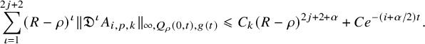 $$ \begin{align} \begin{aligned} \sum_{\iota=1}^{2j+2}(R-\rho)^{\iota} \| \mathfrak{D}^\iota A_{i,p,k} \|_{\infty, Q_\rho(0,t) ,g(t)}&\leqslant C_k(R-\rho)^{2j+2+{\alpha}}+Ce^{-(i+{\alpha}/2)t}. \end{aligned} \end{align} $$
By choosing
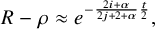 $$ \begin{align} R-\rho\approx e^{-\frac{2i+{\alpha}}{2j+2+{\alpha}}\frac{t}{2}}, \end{align} $$
(which is small), we see that for each
 $1\leqslant \iota \leqslant 2j+2$
,
$1\leqslant \iota \leqslant 2j+2$
,
 $$ \begin{align} \| \mathfrak{D}^\iota A_{i,p,k} \|_{\infty, Q_\rho(0,t),g(t)}\leqslant Ce^{-(2i+{\alpha})(1-\frac{\iota}{2j+2+{\alpha}})\frac{t}2}, \end{align} $$
which is (4.16). Finally for (4.17), by interpolating (4.16) (with
 $\iota =2j+2$
) with (4.18) using Proposition 2.3, we obtain
$\iota =2j+2$
) with (4.18) using Proposition 2.3, we obtain
 $$ \begin{align} (R-\rho)^\iota \|\mathfrak{D}^{2j+2+\iota} A_{i,p,k}\|_{\infty, Q_\rho(0,t),g(t)}\leqslant C(R-\rho)^{\iota+{\alpha}}e^{\iota \frac{t}{2}}+C e^{-(2i+{\alpha})(1-\frac{\iota}{2j+2+{\alpha}})\frac{t}2}. \end{align} $$
By choosing
 $$ \begin{align} R-\rho\approx e^{-\left((2i+{\alpha})(1-\frac{\iota}{2j+2+{\alpha}})+\iota\right)\frac{t}{2(\iota+{\alpha})}}, \end{align} $$
we arrive at
 $$ \begin{align} \|\mathfrak{D}^{2j+2+\iota} A_{i,p,k}\|_{\infty, Q_\rho(0,t),g(t)}\leqslant Ce^{\left(-\frac{{\alpha}(2i+{\alpha})}{\iota+{\alpha}}(1-\frac{2j+2}{2j+2+{\alpha}})+\frac{\iota^2}{\iota+{\alpha}}\right) \frac{t}{2}}. \end{align} $$
This shows (4.17). Thus, to prove Theorem 4.2, it suffices to prove (4.26) when
 $j=0$
, and to prove (4.10), (4.13), (4.15) and (4.18) when
$j=0$
, and to prove (4.10), (4.13), (4.15) and (4.18) when
 $j\geqslant 1$
.
$j\geqslant 1$
.
4.4 Setup of primary blowup quantity
To this end, we denote
 $$ \begin{align} \psi_{j,k}:=\varphi-\underline{\varphi}-\sum_{i=1}^{j}\sum_{p=1}^{N_{i,k}}\mathfrak{G}_{t,k}\left(A_{i,p,k}, G_{i,p,k} \right), \end{align} $$
which by definition satisfies
 $\eta _{j,k}={i\partial \bar \partial }\psi _{j,k}$
. Of course, when
$\eta _{j,k}={i\partial \bar \partial }\psi _{j,k}$
. Of course, when
 $j=0$
, we have by definition
$j=0$
, we have by definition
 $\psi _{0,k}=\varphi -\underline{\varphi }$
. For
$\psi _{0,k}=\varphi -\underline{\varphi }$
. For
 $x=(z,y),x'=(z',y')\in B\times Y$
which are either horizontally or vertically joined and
$x=(z,y),x'=(z',y')\in B\times Y$
which are either horizontally or vertically joined and
 $0<t'<t$
, we consider the quantities
$0<t'<t$
, we consider the quantities
 $$ \begin{align} \mathcal{H}_0(x,x',t,t')=\frac{|{i\partial\bar\partial}\varphi (x,t)-\mathbb{P}_{x'x}{i\partial\bar\partial}\varphi (x',t')|_{g(t)}}{ (d^{g(t)}(x,x')+\sqrt{t-t'})^{\alpha}}, \end{align} $$
and for
 $j\geqslant 1$
,
$j\geqslant 1$
,
 $$ \begin{align} \begin{aligned} \mathcal{H}_{j}(x,x',t,t')&=\frac{|\mathfrak{D}^{2j} {i\partial\bar\partial}\underline{\varphi}(x,t)-\mathbb{P}_{x'x}\mathfrak{D}^{2j}{i\partial\bar\partial}\underline{\varphi}(x',t')|_{g(t)}}{ (d^{g(t)}(x,x')+\sqrt{t-t'})^{\alpha}}\\ &\quad +\frac{|\mathfrak{D}^{2j} (\partial_t\underline{\varphi}+\underline{\varphi})(x,t)-\mathbb{P}_{x'x}\mathfrak{D}^{2j}(\partial_t\underline{\varphi}+\underline{\varphi})(x',t')|_{g(t)}}{ (d^{g(t)}(x,x')+\sqrt{t-t'})^{\alpha}}\\ &\quad +\frac{|\mathfrak{D}^{2j+2}\psi_{j,k}(x,t)-\mathbb{P}_{x'x}\mathfrak{D}^{2j+2} \psi_{j,k}(x',t')|_{g(t)}}{ (d^{g(t)}(x,x')+\sqrt{t-t'})^{\alpha}}\\ &\quad +\sum_{i=1}^j \sum_{p=1}^{N_{i,k}}\sum_{\iota = -2}^{2k} e^{-\iota\frac{t}{2}}\Bigg(\frac{|\mathfrak{D}^{2j+2+\iota} A_{i,p,k}(x,t)-\mathbb{P}_{x'x}(\mathfrak{D}^{2j+2+\iota}A_{i,p,k}(x',t'))|_{g(t)}}{ (d^{g(t)}(x,x')+\sqrt{t-t'})^{\alpha}}\Bigg) \end{aligned} \end{align} $$
as well as
 $$ \begin{align} \mathcal{D}_{j}(x,x',t)=\sup_{t'\in [t-1,t]}\mathcal{H}_{j}(x,x',t,t'), \quad j\geqslant 0. \end{align} $$
For each
 $x=(z,y)\in B\times Y$
and
$x=(z,y)\in B\times Y$
and
 $t\geqslant 0$
, we define the blowup quantity
$t\geqslant 0$
, we define the blowup quantity
 $$ \begin{align} \mu_{j}(x,t)=\left|1-|z| \right|^{2j+{\alpha}} \sup \mathcal{D}_j(x,x',t), \end{align} $$
where the sup is taken over all
 $x'=(z',y')\in B\times Y$
with
$x'=(z',y')\in B\times Y$
with
 $|z'-z|<\frac 14 \left| |z|-1 \right|$
and
$|z'-z|<\frac 14 \left| |z|-1 \right|$
and
 $x'$
is either horizontally or vertically joined with x. We want to show that there is
$x'$
is either horizontally or vertically joined with x. We want to show that there is
 $C>0$
such that for all
$C>0$
such that for all
 $t\geqslant 0$
,
$t\geqslant 0$
,
 $$ \begin{align} \sup_{B\times Y} \mu_{j}(x,t)\leqslant C. \end{align} $$
Since
 $g(t)$
is uniformly comparable to
$g(t)$
is uniformly comparable to
 $g(s)$
if
$g(s)$
if
 $|t-s|<1$
, a bound on
$|t-s|<1$
, a bound on
 $\mu _j$
implies (4.26) when
$\mu _j$
implies (4.26) when
 $j=0$
, and implies (4.10), (4.13), (4.15) and (4.18) when
$j=0$
, and implies (4.10), (4.13), (4.15) and (4.18) when
 $j\geqslant 1$
, and would thus conclude the proof of Theorem 4.2.
$j\geqslant 1$
, and would thus conclude the proof of Theorem 4.2.
Observe that the quantity
 $\mathcal {H}_0$
is closer in spirit to the one used in our earlier works [Reference Hein and Tosatti20, (5.7)] and [Reference Chu and Lee4, (3.10)] (which dealt only with the case
$\mathcal {H}_0$
is closer in spirit to the one used in our earlier works [Reference Hein and Tosatti20, (5.7)] and [Reference Chu and Lee4, (3.10)] (which dealt only with the case
 $j=0$
), rather than the one used in [Reference Hein and Tosatti21, (4.29)] (which dealt with all
$j=0$
), rather than the one used in [Reference Hein and Tosatti21, (4.29)] (which dealt with all
 $j\geqslant 0$
at once).
$j\geqslant 0$
at once).
We now setup the contradiction argument, so suppose that (4.43) fails. We can then find a sequence
 $t_{\ell }>0$
such that
$t_{\ell }>0$
such that
 $\sup _{B\times Y\times [0,t_{\ell }]} \mu _j(x,t)\to +\infty $
as
$\sup _{B\times Y\times [0,t_{\ell }]} \mu _j(x,t)\to +\infty $
as
 $\ell \to +\infty $
. Since the solution of the flow is smooth on any compact time interval, we must have
$\ell \to +\infty $
. Since the solution of the flow is smooth on any compact time interval, we must have
 $t_{\ell }\to +\infty $
. Moreover, there exists
$t_{\ell }\to +\infty $
. Moreover, there exists
 $s_{\ell }\in [0,t_{\ell }]$
such that
$s_{\ell }\in [0,t_{\ell }]$
such that
 $\sup _{B\times Y}\mu _{j}(x,s_{\ell })=\sup _{B\times Y\times [0,t_{\ell }]} \mu _j(x,t)$
. Without loss of generality, we can assume
$\sup _{B\times Y}\mu _{j}(x,s_{\ell })=\sup _{B\times Y\times [0,t_{\ell }]} \mu _j(x,t)$
. Without loss of generality, we can assume
 $s_{\ell }=t_{\ell }\to +\infty $
and
$s_{\ell }=t_{\ell }\to +\infty $
and
 $$ \begin{align} \sup_{B\times Y} \mu_j(x,t_{\ell})\to +\infty. \end{align} $$
For each
 $\ell $
, we choose
$\ell $
, we choose
 $x_{\ell }=(z_{\ell },y_{\ell })\in B\times Y$
such that
$x_{\ell }=(z_{\ell },y_{\ell })\in B\times Y$
such that
 $\mu _j(x_{\ell },t_{\ell })=\sup _{B\times Y} \mu _j(x,t_{\ell })$
. We also define
$\mu _j(x_{\ell },t_{\ell })=\sup _{B\times Y} \mu _j(x,t_{\ell })$
. We also define
 $\lambda _{\ell }$
by
$\lambda _{\ell }$
by
 $$ \begin{align}\lambda_{\ell}^{2j+{\alpha}}:=\sup_{x'} \mathcal{D}_{j}(x_{\ell},x',t_{\ell}), \end{align} $$
so that
 $$ \begin{align} \mu_j(x_{\ell},t_{\ell})= \left| |z_{\ell}|-1\right|^{2j+{\alpha}} \lambda_{\ell}^{2j+{\alpha}}\to +\infty, \end{align} $$
and hence,
 $\lambda _{\ell } \to +\infty $
. Let
$\lambda _{\ell } \to +\infty $
. Let
 $x_{\ell }^{\prime }\in B\times Y$
be the point realizing
$x_{\ell }^{\prime }\in B\times Y$
be the point realizing
 $\sup _{x'} \mathcal {D}_j(x_{\ell },x',t_{\ell })$
and
$\sup _{x'} \mathcal {D}_j(x_{\ell },x',t_{\ell })$
and
 $t_{\ell }^{\prime }\in [t_{\ell }-1,t_{\ell }]$
realizing
$t_{\ell }^{\prime }\in [t_{\ell }-1,t_{\ell }]$
realizing
 $\sup _{t'}\mathcal {H}_j(x_{\ell },x_{\ell }^{\prime },t_{\ell },t')$
. Without loss of generality, we can also assume
$\sup _{t'}\mathcal {H}_j(x_{\ell },x_{\ell }^{\prime },t_{\ell },t')$
. Without loss of generality, we can also assume
 $x_{\ell }\to x_\infty \in \overline {B\times Y}$
.
$x_{\ell }\to x_\infty \in \overline {B\times Y}$
.
Consider the diffeomorphisms
 $$ \begin{align} \Psi_{\ell}: B_{\lambda_{\ell}} \times Y\times [-\lambda_{\ell}^2t_{\ell},0] \to B \times Y\times [0,t_{\ell}], \;\, (z,y,t) = \Psi_{\ell}(\hat{z},\hat{y},\hat{t}) =(\lambda_{\ell}^{-1}\hat{z},\hat{y},t_{\ell}+\lambda_{\ell}^{-2}\hat{t}). \end{align} $$
Let
 $\hat {x}_{\ell }:=(\hat {z}_{\ell },\hat {y}_{\ell })$
, where
$\hat {x}_{\ell }:=(\hat {z}_{\ell },\hat {y}_{\ell })$
, where
 $$ \begin{align} (\hat{z}_{\ell},\hat{y}_{\ell},\hat{t}):=\Psi_{\ell}^{-1}(z_{\ell},y_{\ell},t), \end{align} $$
so that
 $\hat {t}_{\ell }=0, \hat {t}^{\prime }_{\ell }=\lambda _{\ell }^2(t_{\ell }^{\prime }-t_{\ell })$
, and
$\hat {t}_{\ell }=0, \hat {t}^{\prime }_{\ell }=\lambda _{\ell }^2(t_{\ell }^{\prime }-t_{\ell })$
, and
 $\hat {t}=\lambda _{\ell }^2(t-t_{\ell })\in [-\lambda _{\ell }^2 t_{\ell },0]$
. Given a (time-dependent) contravariant
$\hat {t}=\lambda _{\ell }^2(t-t_{\ell })\in [-\lambda _{\ell }^2 t_{\ell },0]$
. Given a (time-dependent) contravariant
 $2$
-tensor
$2$
-tensor
 $\alpha $
(such as
$\alpha $
(such as
 $\omega ^{\bullet }(t), g(t)$
, etc.), we define
$\omega ^{\bullet }(t), g(t)$
, etc.), we define
 $\hat {\alpha }_{\ell }:=\lambda _{\ell }^2\Psi _{\ell }^{*}\alpha $
. Thus, for example,
$\hat {\alpha }_{\ell }:=\lambda _{\ell }^2\Psi _{\ell }^{*}\alpha $
. Thus, for example,
 $\hat \omega _{\ell }^{\bullet }(\hat t)=\lambda _{\ell }^2\Psi _{\ell }^{*} \omega ^{\bullet }(t_{\ell }+\lambda _{\ell }^{-2}\hat t).$
The pullback complex structure will be denoted by
$\hat \omega _{\ell }^{\bullet }(\hat t)=\lambda _{\ell }^2\Psi _{\ell }^{*} \omega ^{\bullet }(t_{\ell }+\lambda _{\ell }^{-2}\hat t).$
The pullback complex structure will be denoted by
 $\hat {J}_{\ell }$
. Given a (time-dependent) scalar function F, we will also denote by
$\hat {J}_{\ell }$
. Given a (time-dependent) scalar function F, we will also denote by
 $\hat {F}_{\ell }:=\Psi _{\ell }^{*}F$
, so that, for example,
$\hat {F}_{\ell }:=\Psi _{\ell }^{*}F$
, so that, for example,
 $\hat {G}_{\ell ,i,p,k}=\Psi _{\ell }^{*}G_{i,p,k}$
. However, for the two functions
$\hat {G}_{\ell ,i,p,k}=\Psi _{\ell }^{*}G_{i,p,k}$
. However, for the two functions
 $A_{i,p,k}$
and
$A_{i,p,k}$
and
 $\varphi $
, we will define instead
$\varphi $
, we will define instead
 $$ \begin{align} \hat A_{\ell,i,p,k}(\hat t):=\lambda_{\ell}^2 \Psi_{\ell}^{*} A_{i,p,k}(t_{\ell}+\lambda_{\ell}^{-2}\hat t),\quad \hat{\varphi }_{\ell}(\hat{t}):=\lambda_{\ell}^2\Psi_{\ell}^{*}\varphi (t_{\ell}+\lambda_{\ell}^{-2}\hat t), \end{align} $$
where
 $\hat {t}\in [-t_{\ell } \lambda _{\ell }^2,0]$
. We define also
$\hat {t}\in [-t_{\ell } \lambda _{\ell }^2,0]$
. We define also
 $$ \begin{align} \delta_{\ell}:=\lambda_{\ell} e^{-\frac{t_{\ell}}{2}}. \end{align} $$
Observe that from (4.31), we have that
 $$ \begin{align} \|\hat A_{\ell,i,p,k}(\hat t)\|_{L^\infty(\hat B_{\lambda_{\ell}})}\leqslant C \delta_{\ell}^2 e^{\frac{-2i+2-{\alpha}}{2}t_{\ell}-\frac{2i+{\alpha}}{2}\lambda_{\ell}^{-2}\hat t} \end{align} $$
for all
 $1\leqslant i\leqslant j$
and
$1\leqslant i\leqslant j$
and
 $1\leqslant p\leqslant N_{i,k}$
and
$1\leqslant p\leqslant N_{i,k}$
and
 $-t_{\ell } \lambda _{\ell }^2\leqslant \hat t\leqslant 0$
. For notational convenience, we will still use
$-t_{\ell } \lambda _{\ell }^2\leqslant \hat t\leqslant 0$
. For notational convenience, we will still use
 $\mathfrak {D}$
and
$\mathfrak {D}$
and
 $\mathbb {P}$
to denote their pullbacks via
$\mathbb {P}$
to denote their pullbacks via
 $\Psi _{\ell }$
. In particular,
$\Psi _{\ell }$
. In particular,
 $\hat \omega _{\ell }^{\bullet }=\hat \omega _{\ell }^\natural +{i\partial \bar \partial } \hat \varphi _{\ell }$
satisfies the following Kähler-Ricci flow
$\hat \omega _{\ell }^{\bullet }=\hat \omega _{\ell }^\natural +{i\partial \bar \partial } \hat \varphi _{\ell }$
satisfies the following Kähler-Ricci flow
 $$ \begin{align} \partial_{\hat t} \hat\omega_{\ell}^{\bullet}=-\textrm{Ric}(\hat\omega_{\ell}^{\bullet})-\lambda_{\ell}^{-2}\hat\omega_{\ell}^{\bullet}, \end{align} $$
and we can equivalently write the complex Monge-Ampère equation (4.1) as
 $$ \begin{align} (\hat \omega_{\ell}^{\bullet})^{m+n}= e^{\partial_{\hat{t}}{\hat\varphi}_{\ell}+\lambda_{\ell}^{-2}\hat\varphi_{\ell}-n \lambda_{\ell}^{-2}\hat t} \binom{m+n}{m} \hat \omega_{\ell,\mathrm{can}} ^m \wedge (\delta_{\ell}^2 \Psi_{\ell}^{*} \omega_F)^n, \end{align} $$
where (following the above convention)
 $\hat \omega _{\ell ,\mathrm {can}}=\lambda _{\ell }^2\Psi _{\ell }^{*} \omega _{\mathrm {can}}$
. It is then straightforward to see that for all
$\hat \omega _{\ell ,\mathrm {can}}=\lambda _{\ell }^2\Psi _{\ell }^{*} \omega _{\mathrm {can}}$
. It is then straightforward to see that for all
 $\ell \geqslant 0$
, we have for
$\ell \geqslant 0$
, we have for
 $j=0,$
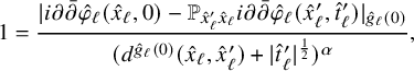 $$ \begin{align} 1=\frac{|{i\partial\bar\partial}\hat\varphi _{\ell}(\hat x_{\ell},0)-\mathbb{P}_{\hat x_{\ell}^{\prime}\hat x_{\ell}}{i\partial\bar\partial}\hat\varphi _{\ell}(\hat x_{\ell}^{\prime},\hat t_{\ell}^{\prime})|_{\hat g_{\ell}(0)}}{ (d^{\hat g_{\ell}(0)}(\hat x_{\ell},\hat x_{\ell}^{\prime})+|\hat t_{\ell}^{\prime}|^{\frac{1}{2}})^{\alpha}}, \end{align} $$
and for
 $j\geqslant 1,$
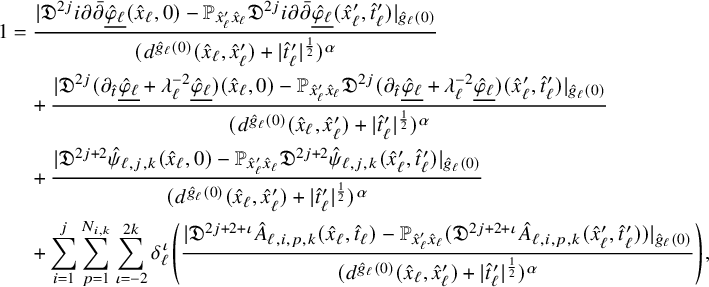 $$ \begin{align} 1&=\frac{|\mathfrak{D}^{2j}{i\partial\bar\partial}\underline{\hat \varphi_{\ell}}(\hat x_{\ell},0)-\mathbb{P}_{\hat x_{\ell}^{\prime}\hat x_{\ell}}\mathfrak{D}^{2j}{i\partial\bar\partial}\underline{\hat\varphi_{\ell}}(\hat x_{\ell}^{\prime},\hat t_{\ell}^{\prime})|_{\hat g_{\ell}(0)}}{ (d^{\hat g_{\ell}(0)}(\hat x_{\ell},\hat x_{\ell}^{\prime})+|\hat t_{\ell}^{\prime}|^{\frac{1}{2}})^{\alpha}}\nonumber\\&\quad +\frac{|\mathfrak{D}^{2j} (\partial_{\hat t}\underline{\hat \varphi_{\ell}}+\lambda_{\ell}^{-2}\underline{\hat \varphi_{\ell}} )(\hat x_{\ell},0)-\mathbb{P}_{\hat x_{\ell}^{\prime}\hat x_{\ell}}\mathfrak{D}^{2j}(\partial_{\hat t}\underline{\hat \varphi_{\ell}}+\lambda_{\ell}^{-2}\underline{\hat \varphi_{\ell}} )(\hat x_{\ell}^{\prime},\hat t_{\ell}^{\prime})|_{\hat g_{\ell}(0)}}{ (d^{\hat g_{\ell}(0)}(\hat x_{\ell},\hat x_{\ell}^{\prime})+|\hat t_{\ell}^{\prime}|^{\frac{1}{2}})^{\alpha}}\nonumber\\&\quad +\frac{|\mathfrak{D}^{2j+2} \hat \psi_{\ell,j,k}(\hat x_{\ell},0)-\mathbb{P}_{\hat x_{\ell}^{\prime}\hat x_{\ell}}\mathfrak{D}^{2j+2} \hat \psi_{\ell,j,k}(\hat x_{\ell}^{\prime},\hat t_{\ell}^{\prime})|_{\hat g_{\ell}(0)}}{ (d^{\hat g_{\ell}(0)}(\hat x_{\ell},\hat x_{\ell}^{\prime})+|\hat t_{\ell}^{\prime}|^{\frac{1}{2}})^{\alpha}}\nonumber\\&\quad +\sum_{i=1}^j \sum_{p=1}^{N_{i,k}}\sum_{\iota = -2}^{2k} \delta_{\ell}^\iota\Bigg(\frac{|\mathfrak{D}^{2j+2+\iota} \hat A_{\ell,i,p,k}(\hat x_{\ell},\hat t_{\ell})- \mathbb{P}_{\hat x_{\ell}^{\prime}\hat x_{\ell}}(\mathfrak{D}^{2j+2+\iota}\hat A_{\ell,i,p,k}(\hat x_{\ell}^{\prime},\hat t_{\ell}^{\prime}))|_{\hat g_{\ell}(0)}}{(d^{\hat g_{\ell}(0)}(\hat x_{\ell},\hat x^{\prime}_{\ell}) +|\hat t_{\ell}^{\prime}|^{\frac{1}{2}})^{\alpha}}\Bigg), \end{align} $$
and
 $\hat {x}^{\prime }_{\ell }$
was chosen to maximize the difference quotients in (4.54) and (4.55) (which we can call
$\hat {x}^{\prime }_{\ell }$
was chosen to maximize the difference quotients in (4.54) and (4.55) (which we can call
 $\hat {\mathcal {D}}_j(\hat {x}_{\ell },\hat {x}',\hat {t}_{\ell })$
) among all points
$\hat {\mathcal {D}}_j(\hat {x}_{\ell },\hat {x}',\hat {t}_{\ell })$
) among all points
 $\hat {x}'=(\hat {z}',\hat {y}')\in B_{\mathbb {C}^m}(\lambda _{\ell })\times Y$
, with
$\hat {x}'=(\hat {z}',\hat {y}')\in B_{\mathbb {C}^m}(\lambda _{\ell })\times Y$
, with
 $|\hat {z}'-\hat {z}_{\ell }|<\frac 14 \left| |\hat {z}_{\ell }|-\lambda _{\ell } \right|$
which are horizontally or vertically joined to
$|\hat {z}'-\hat {z}_{\ell }|<\frac 14 \left| |\hat {z}_{\ell }|-\lambda _{\ell } \right|$
which are horizontally or vertically joined to
 $\hat {x}_{\ell }$
. Moreover, the points
$\hat {x}_{\ell }$
. Moreover, the points
 $\hat {x}_{\ell }$
and
$\hat {x}_{\ell }$
and
 $\hat {t}_{\ell }$
themselves maximize the quantity
$\hat {t}_{\ell }$
themselves maximize the quantity
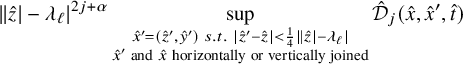 $$ \begin{align} \left\|\hat{z}|-\lambda_{\ell} \right|^{2j+{\alpha}} \sup_{\substack{\hat{x}'=(\hat{z}',\hat{y}')\ s.t.\ |\hat{z}'-\hat{z}|<\frac{1}{4}\|\hat{z}|-\lambda_{\ell}|\\\hat{x}'\ \mathrm{and}\ \hat{x}\ \mathrm{horizontally}\ \mathrm{or}\ \mathrm{vertically}\ \mathrm{joined}}} \hat{\mathcal{D}}_j(\hat{x},\hat{x}',\hat{t}) \end{align} $$
among all
 $\hat {x}=(\hat z,\hat y)\in B_{\mathbb {C}^m}(\lambda _{\ell })\times Y$
and
$\hat {x}=(\hat z,\hat y)\in B_{\mathbb {C}^m}(\lambda _{\ell })\times Y$
and
 $\hat t\in [-t_{\ell }\lambda _{\ell }^2,0]$
; hence, for all such
$\hat t\in [-t_{\ell }\lambda _{\ell }^2,0]$
; hence, for all such
 $\hat {x},\hat {x}',\hat {t}$
, we have
$\hat {x},\hat {x}',\hat {t}$
, we have
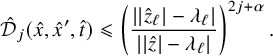 $$ \begin{align} \hat{ \mathcal{D}}_{j} (\hat x,\hat x',\hat t) \leqslant \left(\frac{\left| |\hat z_{\ell}|-\lambda_{\ell}\right|}{\left| |\hat z|-\lambda_{\ell}\right|} \right)^{2j+{\alpha}}. \end{align} $$
Using
 $\left| |\hat z_{\ell }|-\lambda _{\ell }\right|=\lambda _{\ell } \left| |z_{\ell }|-1\right|\to +\infty $
(hence the pointed limit centered at
$\left| |\hat z_{\ell }|-\lambda _{\ell }\right|=\lambda _{\ell } \left| |z_{\ell }|-1\right|\to +\infty $
(hence the pointed limit centered at
 $\hat x_{\ell }$
will be complete) and
$\hat x_{\ell }$
will be complete) and
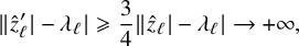 $$ \begin{align} \|\hat{z}^{\prime}_{\ell}|-\lambda_{\ell}|\geqslant\frac{3}{4}\|\hat{z}_{\ell}|-\lambda_{\ell}|\to+\infty, \end{align} $$
together with the triangle inequality, we see from (4.57) that there exists
 $C>0$
such that for any fixed
$C>0$
such that for any fixed
 $R>0$
, there exists
$R>0$
, there exists
 $\ell _R\in \mathbb {N}$
such that for all
$\ell _R\in \mathbb {N}$
such that for all
 $\ell \geqslant \ell _R$
and
$\ell \geqslant \ell _R$
and
 $\hat {z}^{\bullet }_{\ell }=\hat {z}_{\ell }$
or
$\hat {z}^{\bullet }_{\ell }=\hat {z}_{\ell }$
or
 $\hat {z}^{\prime }_{\ell }$
, we have
$\hat {z}^{\prime }_{\ell }$
, we have
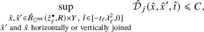 $$ \begin{align} \sup_{\substack{\hat{x},\hat{x}' \in \hat{B}_{\mathbb{C}^m}(\hat{z}^{\bullet}_{\ell},R)\times Y,\ \hat t\in [-t_{\ell}\lambda_{\ell}^2,0]\\\hat{x}'\ \mathrm{and}\ \hat{x}\ \mathrm{horizontally}\ \mathrm{or}\ \mathrm{vertically}\ \mathrm{joined}}} \hat{ \mathcal{D}}_{j} (\hat x,\hat x',\hat t) \leqslant C, \end{align} $$
where here and in the following, the hat decoration over
 $B_{\mathbb {C}^m}$
is just to remind the reader that we are in the hat picture. This in particular implies there exists
$B_{\mathbb {C}^m}$
is just to remind the reader that we are in the hat picture. This in particular implies there exists
 $C>0$
so that for all fixed R,
$C>0$
so that for all fixed R,
 $\hat t\in [-t_{\ell }\lambda _{\ell }^2,0]$
and all sufficiently large
$\hat t\in [-t_{\ell }\lambda _{\ell }^2,0]$
and all sufficiently large
 $\ell $
, we have for
$\ell $
, we have for
 $j=0,$
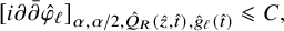 $$ \begin{align} [{i\partial\bar\partial}\hat\varphi _{\ell}]_{{\alpha},{\alpha}/2,\hat Q_R(\hat z,\hat t),\hat g_{\ell}(\hat t)}\leqslant C, \end{align} $$
and for
 $j\geqslant 1,$
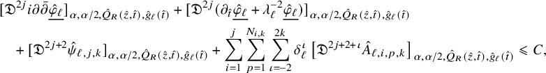 $$ \begin{align} \begin{aligned} &[\mathfrak{D}^{2j} {i\partial\bar\partial} \underline{\hat \varphi_{\ell}}]_{{\alpha},{\alpha}/2,\hat Q_R(\hat z,\hat t),\hat g_{\ell}(\hat t)}+ [\mathfrak{D}^{2j} (\partial_{\hat t}\underline{\hat \varphi_{\ell}}+\lambda_{\ell}^{-2}\underline{\hat \varphi_{\ell}})]_{{\alpha},{\alpha}/2,\hat Q_R(\hat z,\hat t),\hat g_{\ell}(\hat t)}\\&\quad + [\mathfrak{D}^{2j+2} \hat \psi_{\ell,j,k} ]_{{\alpha},{\alpha}/2,\hat Q_R(\hat z,\hat t),\hat g_{\ell}(\hat t)}+\sum_{i=1}^j \sum_{p=1}^{N_{i,k}}\sum_{\iota = -2}^{2k} \delta_{\ell}^\iota\left[\mathfrak{D}^{2j+2+\iota} \hat A_{\ell,i,p,k}\right]_{{\alpha},{\alpha}/2,\hat Q_R(\hat z,\hat t),\hat g_{\ell}(\hat t)}\leqslant C, \end{aligned} \end{align} $$
where
 $\hat Q_R(\hat z,\hat t)=\left(B_{\mathbb {C}^m}(\hat z,R)\times Y\right)\times [-R^2+\hat t,\hat t]$
with
$\hat Q_R(\hat z,\hat t)=\left(B_{\mathbb {C}^m}(\hat z,R)\times Y\right)\times [-R^2+\hat t,\hat t]$
with
 $\hat z$
being either
$\hat z$
being either
 $\hat z_{\ell }$
or
$\hat z_{\ell }$
or
 $\hat z_{\ell }^{\prime }$
.
$\hat z_{\ell }^{\prime }$
.
When
 $j=0$
we will need the following ‘non-cancellation’ inequality
$j=0$
we will need the following ‘non-cancellation’ inequality
 $$ \begin{align} [{i\partial\bar\partial}\underline{\hat{\varphi }_{\ell}}]_{{\alpha},{\alpha}/2,\hat Q_R(\hat z,\hat t),\hat g_{\ell}(\hat t)}\leqslant C[{i\partial\bar\partial}\hat{\varphi }_{\ell}]_{{\alpha},{\alpha}/2, \textrm{base},\hat Q_R(\hat z,\hat t),g_X} +C\left(\frac{R}{\lambda_{\ell}}\right)^{1-\alpha}\|{i\partial\bar\partial}\hat{\varphi }_{\ell}\|_{\infty, \hat Q_R(\hat z,\hat t),g_X}, \end{align} $$
which is again straightforward to prove using [Reference Hein and Tosatti21, (4.215)], and plugging in the Hölder bound in (4.60) and the
 $L^\infty $
bound
$L^\infty $
bound
 $\|{i\partial \bar \partial }\hat {\varphi }_{\ell }\|_{\infty , \hat Q_R(\hat z,\hat t),\hat {g}_{\ell }(\hat {t})}=o(1)$
which comes from Lemma 4.1 (iii), we see that
$\|{i\partial \bar \partial }\hat {\varphi }_{\ell }\|_{\infty , \hat Q_R(\hat z,\hat t),\hat {g}_{\ell }(\hat {t})}=o(1)$
which comes from Lemma 4.1 (iii), we see that
 $$ \begin{align} [{i\partial\bar\partial}\underline{\hat\varphi _{\ell}}]_{{\alpha},{\alpha}/2,\hat Q_R(\hat z,\hat t),\hat g_{\ell}(\hat t)}\leqslant C, \end{align} $$
and combining this with (4.60), using that
 $\hat {\eta }_{0,k}={i\partial \bar \partial }\hat {\psi }_{\ell ,0,k}={i\partial \bar \partial }\hat {\varphi }_{\ell }-{i\partial \bar \partial }\underline{\hat {\varphi }_{\ell }}$
, and using the triangle inequality and the boundedness of
$\hat {\eta }_{0,k}={i\partial \bar \partial }\hat {\psi }_{\ell ,0,k}={i\partial \bar \partial }\hat {\varphi }_{\ell }-{i\partial \bar \partial }\underline{\hat {\varphi }_{\ell }}$
, and using the triangle inequality and the boundedness of
 $\mathbb {P}$
, we get
$\mathbb {P}$
, we get
 $$ \begin{align} [{i\partial\bar\partial}\underline{\hat\varphi _{\ell}}]_{{\alpha},{\alpha}/2,\hat Q_R(\hat z,\hat t),\hat g_{\ell}(\hat t)}+[{i\partial\bar\partial}\hat{\psi}_{\ell,0,k}]_{{\alpha},{\alpha}/2,\hat Q_R(\hat z,\hat t),\hat g_{\ell}(\hat t)}\leqslant C. \end{align} $$
After passing to subsequence, we will split the rest of the proof into three cases, according to the behavior of
 $\delta _{\ell }=\lambda _{\ell } e^{-t_{\ell }/2}$
: Case 1:
$\delta _{\ell }=\lambda _{\ell } e^{-t_{\ell }/2}$
: Case 1:
 $\delta _{\ell }\to +\infty $
, Case 2:
$\delta _{\ell }\to +\infty $
, Case 2:
 $\delta _{\ell }\to \delta _\infty>0$
and Case 3:
$\delta _{\ell }\to \delta _\infty>0$
and Case 3:
 $\delta _{\ell }\to 0$
.
$\delta _{\ell }\to 0$
.
4.5 Non-escaping property
In this subsection, we will show that in Cases 2 and 3, the distance between the two blowup points
 $\hat {x}_{\ell }$
and
$\hat {x}_{\ell }$
and
 $\hat x_{\ell }^{\prime }$
will not go to infinity. This proof does not apply to Case 1 (at least when
$\hat x_{\ell }^{\prime }$
will not go to infinity. This proof does not apply to Case 1 (at least when
 $j\geqslant 1$
), but we will nevertheless establish the same result in that case in (4.97) below.
$j\geqslant 1$
), but we will nevertheless establish the same result in that case in (4.97) below.
Proposition 4.4. Suppose
 $\delta _{\ell }\leqslant C$
for some
$\delta _{\ell }\leqslant C$
for some
 $C>0$
. Then there exists
$C>0$
. Then there exists
 $C'>0$
such that for all
$C'>0$
such that for all
 $\ell>0$
,
$\ell>0$
,
 $$ \begin{align} d^{\hat g_{\ell}(0)}(\hat x_{\ell},\hat x_{\ell}^{\prime})+|\hat t_{\ell}^{\prime}|^{\frac{1}{2}}\leqslant C'. \end{align} $$
Proof. First, we can easily deal with the case
 $j=0$
. By Lemma 4.1 (iii), we know that
$j=0$
. By Lemma 4.1 (iii), we know that
 $$ \begin{align} \sup_{B\times Y\times [t-1,t]}|{i\partial\bar\partial}\varphi |_{g(t)}=o(1), \end{align} $$
which implies
 $$ \begin{align} \|{i\partial\bar\partial}\hat{\varphi }_{\ell}\|_{\infty,\hat Q_\rho(\hat z,\hat t),g_{\ell}(\hat t)}=o(1) \end{align} $$
as
 $\ell \to \infty $
, for fixed
$\ell \to \infty $
, for fixed
 $\hat {z},\hat {t},\rho $
, and applying this to
$\hat {z},\hat {t},\rho $
, and applying this to
 $\hat {z}=\hat {z}_{\ell }$
or
$\hat {z}=\hat {z}_{\ell }$
or
 $\hat {z}^{\prime }_{\ell }$
and
$\hat {z}^{\prime }_{\ell }$
and
 $\hat {t}=0$
or
$\hat {t}=0$
or
 $\hat {t}^{\prime }_{\ell }$
, we see that the numerator on the RHS of (4.54) is going to zero, which gives us the even stronger statement that
$\hat {t}^{\prime }_{\ell }$
, we see that the numerator on the RHS of (4.54) is going to zero, which gives us the even stronger statement that
 $$ \begin{align} d^{\hat g_{\ell}(0)}(\hat x_{\ell},\hat x_{\ell}^{\prime})+|\hat t_{\ell}^{\prime}|^{\frac{1}{2}}=o(1), \end{align} $$
and for
 $j=0$
, we do not even need the assumption that
$j=0$
, we do not even need the assumption that
 $\delta _{\ell }\leqslant C$
.
$\delta _{\ell }\leqslant C$
.
Next, we assume
 $j\geqslant 1$
. The argument is a modification of [Reference Hein and Tosatti21, Proposition 4.5], and the goal is to estimate each of the terms in the blowup quantity in (4.55). In the following, we denote
$j\geqslant 1$
. The argument is a modification of [Reference Hein and Tosatti21, Proposition 4.5], and the goal is to estimate each of the terms in the blowup quantity in (4.55). In the following, we denote
 $\hat Q_R(\hat z,\hat t)=\left(B_{\mathbb {C}^m}(\hat z,R)\times Y\right)\times [-R^2+\hat t,\hat t]$
with
$\hat Q_R(\hat z,\hat t)=\left(B_{\mathbb {C}^m}(\hat z,R)\times Y\right)\times [-R^2+\hat t,\hat t]$
with
 $\hat z$
being either
$\hat z$
being either
 $\hat z_{\ell }$
or
$\hat z_{\ell }$
or
 $\hat z_{\ell }^{\prime }$
and
$\hat z_{\ell }^{\prime }$
and
 $\hat t$
is either
$\hat t$
is either
 $\hat t_{\ell }=0$
or
$\hat t_{\ell }=0$
or
 $\hat t_{\ell }^{\prime }$
.
$\hat t_{\ell }^{\prime }$
.
We first handle the terms involving
 $A_{\ell ,i,p,k}$
. Recall from (4.61) that for all
$A_{\ell ,i,p,k}$
. Recall from (4.61) that for all
 $-2\leqslant \iota \leqslant 2k$
and each given
$-2\leqslant \iota \leqslant 2k$
and each given
 $R>0$
,
$R>0$
,
 $$ \begin{align} \left[\mathfrak{D}^{2j+2+\iota} \hat A_{\ell,i,p,k}\right]_{{\alpha},{\alpha}/2,\hat Q_R(\hat z,\hat t),\hat g_{\ell}(\hat t)}\leqslant C\delta_{\ell}^{-\iota}, \end{align} $$
while from (4.51),
 $$ \begin{align} \|\hat A_{\ell,i,p,k}\|_{\infty,\hat Q_R(\hat z,\hat t)}\leqslant C \delta_{\ell}^2 e^{\frac{-2i+2-{\alpha}}{2}t_{\ell}+\frac{2i+{\alpha}}{2}\lambda_{\ell}^{-2}(R^2-\hat t)}\leqslant C \delta_{\ell}^2 e^{\frac{-2i+2-{\alpha}}{2}t_{\ell}} \end{align} $$
since
 $\hat {t}=0$
or
$\hat {t}=0$
or
 $\hat {t}_{\ell }^{\prime }$
satisfies
$\hat {t}_{\ell }^{\prime }$
satisfies
 $\hat {t}\geqslant -\lambda _{\ell }^2$
. By Proposition 2.3, for all
$\hat {t}\geqslant -\lambda _{\ell }^2$
. By Proposition 2.3, for all
 $1\leqslant r\leqslant 2j$
,
$1\leqslant r\leqslant 2j$
,
 $$ \begin{align} \begin{aligned} (R-\rho)^r \|\mathfrak{D}^r\hat A_{\ell,i,p,k}\|_{\infty,\hat Q_\rho(\hat z,\hat t),\hat g_{\ell}(\hat t)}\leqslant C(R-\rho)^{2j+{\alpha}}\delta_{\ell}^2+C \delta_{\ell}^2 e^{\frac{-2i+2-{\alpha}}{2}t_{\ell}}. \end{aligned} \end{align} $$
We choose
 $$ \begin{align} R-\rho\approx \left( e^{\frac{-2i+2-{\alpha}}{2}t_{\ell}}\right)^{\frac{1}{2j+{\alpha}}}, \end{align} $$
which is small for any given R. We get for all
 $0\leqslant r\leqslant 2j$
that
$0\leqslant r\leqslant 2j$
that
 $$ \begin{align} \|\mathfrak{D}^r\hat A_{\ell,i,p,k}\|_{\infty,\hat Q_\rho(\hat z,\hat t),\hat g_{\ell}(\hat t)}\leqslant C\delta_{\ell}^2\left( e^{\frac{-2i+2-{\alpha}}{2}t_{\ell}}\right)^{1-\frac{r}{2j+{\alpha}}}=o(1), \end{align} $$
where
 $\hat t$
is either
$\hat t$
is either
 $\hat t_{\ell }=0$
or
$\hat t_{\ell }=0$
or
 $\hat t_{\ell }^{\prime }$
.
$\hat t_{\ell }^{\prime }$
.
If we let
 $r=\iota +2>0$
, then for
$r=\iota +2>0$
, then for
 $0<r\leqslant 2k+2$
, we can interpolate again, using (4.69), and get
$0<r\leqslant 2k+2$
, we can interpolate again, using (4.69), and get
 $$ \begin{align} \begin{aligned} (R-\rho)^r \|\mathfrak{D}^{2j+r}\hat A_{\ell,i,p,k}\|_{\infty,\hat Q_\rho(\hat z,\hat t),\hat g_{\ell}(\hat t)}\leqslant C(R-\rho)^{r+{\alpha}}\delta_{\ell}^{-r+2}+C\delta_{\ell}^2\left( e^{\frac{-2i+2-{\alpha}}{2}t_{\ell}}\right)^{\frac{{\alpha}}{2j+{\alpha}}}. \end{aligned} \end{align} $$
By taking
 $$ \begin{align} R-\rho\approx \left(\delta_{\ell}^r\left( e^{\frac{-2i+2-{\alpha}}{2}t_{\ell}}\right)^{\frac{{\alpha}}{2j+{\alpha}}}\right)^{\frac{1}{r+{\alpha}}}, \end{align} $$
which is small thanks to our assumption that
 $\delta _{\ell }\leqslant C$
, we conclude that for all
$\delta _{\ell }\leqslant C$
, we conclude that for all
 $0<r\leqslant 2k+2$
,
$0<r\leqslant 2k+2$
,
 $$ \begin{align} \delta_{\ell}^{r-2} \|\mathfrak{D}^{2j+r}\hat A_{\ell,i,p,k}\|_{\infty,\hat Q_\rho(\hat z,\hat t),\hat g_{\ell}(\hat t)}\leqslant C \left(\delta_{\ell}^r\left( e^{\frac{-2i+2-{\alpha}}{2}t_{\ell}}\right)^{\frac{{\alpha}}{2j+{\alpha}}}\right)^{\frac{{\alpha}}{r+{\alpha}}} =o(1). \end{align} $$
Applying (4.73) and (4.76) to balls centered at
 $(\hat z_{\ell },\hat t_{\ell })$
and
$(\hat z_{\ell },\hat t_{\ell })$
and
 $(\hat z_{\ell }^{\prime },\hat t_{\ell }^{\prime })$
(of any radius – for example,
$(\hat z_{\ell }^{\prime },\hat t_{\ell }^{\prime })$
(of any radius – for example,
 $1$
), together with the boundedness of operator norm of
$1$
), together with the boundedness of operator norm of
 $\mathbb {P}$
from [Reference Hein and Tosatti21, §2.1.1], this gives
$\mathbb {P}$
from [Reference Hein and Tosatti21, §2.1.1], this gives
 $$ \begin{align} \sum_{i=1}^j \sum_{p=1}^{N_{i,k}}\sum_{\iota = -2}^{2k} \delta_{\ell}^\iota\Bigg({|\mathfrak{D}^{2j+2+\iota} \hat A_{\ell,i,p,k}(\hat x_{\ell},0)- \mathbb{P}_{\hat x_{\ell}^{\prime}\hat x_{\ell}}(\mathfrak{D}^{2j+2+\iota}\hat A_{\ell,i,p,k}(\hat x_{\ell}^{\prime},\hat t_{\ell}^{\prime}))|_{\hat g_{\ell}(0)}}\Bigg)=o(1). \end{align} $$
We now treat
 $\hat \psi _{\ell ,j,k}$
which has fiberwise average zero. By Proposition 2.6 (in case
$\hat \psi _{\ell ,j,k}$
which has fiberwise average zero. By Proposition 2.6 (in case
 $\delta _{\ell }$
does not converge to
$\delta _{\ell }$
does not converge to
 $0$
, we choose
$0$
, we choose
 $\rho $
to be sufficiently large) and (4.61), we have
$\rho $
to be sufficiently large) and (4.61), we have
 $$ \begin{align} \|\mathfrak{D}^{2j+2} \hat \psi_{\ell,j,k}\|_{\infty,\hat Q_\rho(\hat z,\hat t),\hat g_{\ell}(\hat t)}\leqslant C\delta_{\ell}^{\alpha}. \end{align} $$
Applying this to balls centered at
 $\hat z_{\ell }$
and
$\hat z_{\ell }$
and
 $\hat z_{\ell }^{\prime }$
and invoking [Reference Hein and Tosatti21, §2.1.1] again, we have
$\hat z_{\ell }^{\prime }$
and invoking [Reference Hein and Tosatti21, §2.1.1] again, we have
 $$ \begin{align} \begin{aligned} {|\mathfrak{D}^{2j+2} \hat \psi_{\ell,j,k}(\hat x_{\ell},0)-\mathbb{P}_{\hat x_{\ell}^{\prime}\hat x_{\ell}}\mathfrak{D}^{2j+2} \hat \psi_{\ell,j,k}(\hat x_{\ell}^{\prime},\hat t_{\ell}^{\prime})|_{\hat g_{\ell}(0)}}\leqslant C\delta_{\ell}^{\alpha}. \end{aligned} \end{align} $$
It remains to consider the fiberwise average of the potential (i.e.,
 $\underline{\hat \varphi _{\ell }}$
). Recalling (4.66) and taking fiber average (using the fiber integration argument in [Reference Tosatti38, p.436]) gives in particular
$\underline{\hat \varphi _{\ell }}$
). Recalling (4.66) and taking fiber average (using the fiber integration argument in [Reference Tosatti38, p.436]) gives in particular
 $$ \begin{align} \|{i\partial\bar\partial}\underline{\varphi }\|_{\infty, B\times [t-1,t], g_{\mathbb{C}^m}}=o(1), \end{align} $$
as
 $t\to +\infty $
, which implies
$t\to +\infty $
, which implies
 $$ \begin{align} \|{i\partial\bar\partial}\underline{\hat{\varphi }_{\ell}}\|_{\infty,\hat Q_\rho(\hat z,\hat t),g_{\ell}(\hat t)}=o(1), \end{align} $$
as
 $\ell \to \infty $
, for fixed
$\ell \to \infty $
, for fixed
 $\hat {z},\hat {t},\rho $
, and interpolating between this and (4.61) gives
$\hat {z},\hat {t},\rho $
, and interpolating between this and (4.61) gives
 $$ \begin{align} \|\mathfrak{D}^{2j}{i\partial\bar\partial}\underline{\hat \varphi_{\ell}}\|_{\infty, \hat Q_\rho(\hat z,\hat t),g_{\ell}(\hat t)}=o(1) \end{align} $$
for
 $\hat {z}=\hat {z}_{\ell }$
or
$\hat {z}=\hat {z}_{\ell }$
or
 $\hat {z}^{\prime }_{\ell }$
and
$\hat {z}^{\prime }_{\ell }$
and
 $\hat {t}=0$
or
$\hat {t}=0$
or
 $\hat {t}^{\prime }_{\ell }$
. Using again the boundedness of the operator norm of
$\hat {t}^{\prime }_{\ell }$
. Using again the boundedness of the operator norm of
 $\mathbb {P}$
, this implies that
$\mathbb {P}$
, this implies that
 $$ \begin{align} |\mathfrak{D}^{2j}{i\partial\bar\partial}\underline{\hat \varphi_{\ell}}(\hat x_{\ell},0)-\mathbb{P}_{\hat x_{\ell}^{\prime}\hat x_{\ell}}\mathfrak{D}^{2j}{i\partial\bar\partial}\underline{\hat\varphi_{\ell}}(\hat x_{\ell}^{\prime},\hat t_{\ell}^{\prime})|_{\hat g_{\ell}(0)}=o(1). \end{align} $$
Similarly, from Lemma 4.1 (ii) and taking fiber average, we know that
 $$ \begin{align} \sup_{B\times Y\times [t-1,t]}|\partial_t\underline{\varphi }+\underline{\varphi }|=o(1), \end{align} $$
as
 $t\to +\infty $
, which implies
$t\to +\infty $
, which implies
 $$ \begin{align} \|\partial_{\hat{t}}\underline{\hat \varphi_{\ell}}+\lambda_{\ell}^{-2}\underline{\hat \varphi_{\ell}}\|_{\infty,\hat Q_\rho(\hat z,\hat t),g_{\ell}(\hat t)}=o(1), \end{align} $$
as
 $\ell \to \infty $
, for fixed
$\ell \to \infty $
, for fixed
 $\hat {z},\hat {t},\rho $
, and again interpolating between this and (4.61) gives
$\hat {z},\hat {t},\rho $
, and again interpolating between this and (4.61) gives
 $$ \begin{align} \|\mathfrak{D}^{2j}(\partial_{\hat t}\underline{\hat \varphi_{\ell}}+\lambda_{\ell}^{-2}\underline{\hat \varphi_{\ell}} )\|_{\infty, \hat Q_\rho(\hat z,\hat t),g_{\ell}(\hat t)}=o(1), \end{align} $$
for
 $\hat {z}=\hat {z}_{\ell }$
or
$\hat {z}=\hat {z}_{\ell }$
or
 $\hat {z}^{\prime }_{\ell }$
and
$\hat {z}^{\prime }_{\ell }$
and
 $\hat {t}=0$
or
$\hat {t}=0$
or
 $\hat {t}^{\prime }_{\ell }$
, and hence,
$\hat {t}^{\prime }_{\ell }$
, and hence,
 $$ \begin{align} {|\mathfrak{D}^{2j} (\partial_{\hat t}\underline{\hat \varphi_{\ell}}+\lambda_{\ell}^{-2}\underline{\hat \varphi_{\ell}} )(\hat x_{\ell},0)-\mathbb{P}_{\hat x_{\ell}^{\prime}\hat x_{\ell}}\mathfrak{D}^{2j}(\partial_{\hat t}\underline{\hat \varphi_{\ell}}+\lambda_{\ell}^{-2}\underline{\hat \varphi_{\ell}} )(\hat x_{\ell}^{\prime},\hat t_{\ell}^{\prime})|_{\hat g_{\ell}(0)}}=o(1). \end{align} $$
Combining (4.55) with (4.77), (4.79), (4.83) and (4.87), we obtain the desired bound (4.65).
We are now in position to study the flows obtained as complete pointed limits of
 $$ \begin{align} \left( \hat B_{\mathbb{C}^m}(\hat z_{\ell},\lambda_{\ell})\times Y, \hat g_{\ell}(\hat{t}),\hat x_{\ell}\right), \end{align} $$
as
 $\ell \to +\infty $
, where as usual
$\ell \to +\infty $
, where as usual
 $\hat {t}\in [-\lambda _{\ell }^2t_{\ell },0]$
. By translation, we can assume
$\hat {t}\in [-\lambda _{\ell }^2t_{\ell },0]$
. By translation, we can assume
 $\hat x_{\ell }=(\hat z_{\ell },\hat y_{\ell })=(0,\hat y_{\ell })\in \mathbb {C}^m\times Y$
and
$\hat x_{\ell }=(\hat z_{\ell },\hat y_{\ell })=(0,\hat y_{\ell })\in \mathbb {C}^m\times Y$
and
 $\hat y_{\ell }\to \hat y_\infty \in Y$
by compactness of Y after passing to a subsequence.
$\hat y_{\ell }\to \hat y_\infty \in Y$
by compactness of Y after passing to a subsequence.
4.6 Blowup analysis in Case 1:
$\delta _{\ell }\to +\infty $

In this case, the metrics
 $\hat {g_{\ell }}(0)$
are blowing up in the fiber directions, so that their pointed blowup limit (modulo local diffeomorphisms that stretch the fibers) would be
$\hat {g_{\ell }}(0)$
are blowing up in the fiber directions, so that their pointed blowup limit (modulo local diffeomorphisms that stretch the fibers) would be
 $\mathbb {C}^{m+n}$
. While this is the approach taken in our earlier works [Reference Chu and Lee4, Reference Fong and Lee11, Reference Hein and Tosatti20], it turns out that we need a different approach instead (at least when
$\mathbb {C}^{m+n}$
. While this is the approach taken in our earlier works [Reference Chu and Lee4, Reference Fong and Lee11, Reference Hein and Tosatti20], it turns out that we need a different approach instead (at least when
 $j\geqslant 1$
). So, following [Reference Hein and Tosatti21], we consider the diffeomorphisms
$j\geqslant 1$
). So, following [Reference Hein and Tosatti21], we consider the diffeomorphisms
 $$ \begin{align} \Xi_{\ell}: B_{e^{\frac{t_{\ell}}{2}}} \times Y\times [-e^{t_{\ell}}t_{\ell},0] \to B_{\lambda_{\ell}} \times Y\times [-\lambda_{\ell}^2t_{\ell},0], \;\, (\hat{z},\hat{y},\hat{t}) = \Xi_{\ell}(\check{z},\check{y},\check{t}) =(\delta_{\ell}\check{z},\check{y},\delta_{\ell}^2\check{t}), \end{align} $$
pull back time-dependent
 $2$
-tensors via
$2$
-tensors via
 $\Xi _{\ell }$
, rescale them by
$\Xi _{\ell }$
, rescale them by
 $\delta _{\ell }^{-2}$
and denote the new tensors with a check, so, for example,
$\delta _{\ell }^{-2}$
and denote the new tensors with a check, so, for example,
 $\check \omega ^{\bullet }_{\ell }(\check t)=\delta _{\ell }^{-2} \Xi _{\ell }^{*}\hat \omega _{\ell }^{\bullet }(\delta _{\ell }^2 \check t)$
. We also apply the same pullback and rescaling procedure to the scalar functions
$\check \omega ^{\bullet }_{\ell }(\check t)=\delta _{\ell }^{-2} \Xi _{\ell }^{*}\hat \omega _{\ell }^{\bullet }(\delta _{\ell }^2 \check t)$
. We also apply the same pullback and rescaling procedure to the scalar functions
 $\hat {A}_{\ell ,i,p,k}$
and
$\hat {A}_{\ell ,i,p,k}$
and
 $\hat {\varphi }_{\ell }$
.
$\hat {\varphi }_{\ell }$
.
In this case,
 $\check g_{\ell }(\check {t})$
is locally uniformly Euclidean in space-time and
$\check g_{\ell }(\check {t})$
is locally uniformly Euclidean in space-time and
 $\check \omega _{\ell }^{\bullet } $
satisfies the Kähler-Ricci flow equation
$\check \omega _{\ell }^{\bullet } $
satisfies the Kähler-Ricci flow equation
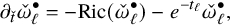 $$ \begin{align}\partial_{\check t}\check \omega_{\ell}^{\bullet} = -\textrm{Ric}(\check \omega_{\ell}^{\bullet} )-e^{-t_{\ell}}\check \omega_{\ell}^{\bullet} ,\end{align} $$
and the Monge-Ampère equation (4.53) becomes
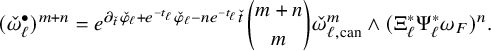 $$ \begin{align} (\check \omega_{\ell}^{\bullet})^{m+n}= e^{\partial_{\check{t}}{\check\varphi}_{\ell}+e^{-t_{\ell}}\check\varphi_{\ell}-n e^{-t_{\ell}}\check t} \binom{m+n}{m} \check \omega_{\ell,\mathrm{can}} ^m \wedge (\Xi_{\ell}^{*} \Psi_{\ell}^{*} \omega_F)^n. \end{align} $$
Thanks to Lemma 4.1 (i), we know that
 $\check \omega _{\ell }^{\bullet } (\check t)$
is uniformly equivalent to
$\check \omega _{\ell }^{\bullet } (\check t)$
is uniformly equivalent to
 $$ \begin{align} \check \omega_{\ell}^\natural(\check t)=(1-e^{-t_{\ell}-e^{-t_{\ell}}\check t}) \check \omega_{\ell,\mathrm{can}}+e^{-e^{-t_{\ell}}\check t}\Xi_{\ell}^{*}\Psi_{\ell}^{*}\omega_F, \end{align} $$
which in turn is locally uniformly equivalent to the Euclidean metric. The pullback of the complex structure also converges locally uniformly smoothly to the Euclidean product complex structure due to the stretching. We want to apply the local higher order estimates in [Reference Chu and Lee4, Proposition 2.1] on
 $\check Q_1(\check z_{\ell },0)$
and
$\check Q_1(\check z_{\ell },0)$
and
 $\check Q_1(\check z_{\ell }^{\prime },\check t_{\ell }^{\prime })$
, but we do not know whether
$\check Q_1(\check z_{\ell }^{\prime },\check t_{\ell }^{\prime })$
, but we do not know whether
 $\check {B}_1(\check {z}_{\ell }),\check {B}_1(\check {z}^{\prime }_{\ell })$
are contained in
$\check {B}_1(\check {z}_{\ell }),\check {B}_1(\check {z}^{\prime }_{\ell })$
are contained in
 $B_{e^{\frac {t_{\ell }}{2}}}$
, as we do not have any relation between
$B_{e^{\frac {t_{\ell }}{2}}}$
, as we do not have any relation between
 $\delta _{\ell }$
and
$\delta _{\ell }$
and
 $\|\hat {z}_{\ell }|-\lambda _{\ell }|$
. However, these are compactly contained in the slightly larger ball
$\|\hat {z}_{\ell }|-\lambda _{\ell }|$
. However, these are compactly contained in the slightly larger ball
 $B_{(1+\sigma )e^{\frac {t_{\ell }}{2}}}$
for any fixed
$B_{(1+\sigma )e^{\frac {t_{\ell }}{2}}}$
for any fixed
 $\sigma>0$
and all
$\sigma>0$
and all
 $\ell $
sufficiently large, and we may assume without loss that
$\ell $
sufficiently large, and we may assume without loss that
 $\check \omega _{\ell }^{\bullet } (\check t)$
is uniformly equivalent to Euclidean on
$\check \omega _{\ell }^{\bullet } (\check t)$
is uniformly equivalent to Euclidean on
 $B_{(1+\sigma )e^{\frac {t_{\ell }}{2}}}\times Y\times [-(1+\sigma )^2e^{t_{\ell }}t_{\ell },0]$
. Thus, the local higher order estimates give us uniform
$B_{(1+\sigma )e^{\frac {t_{\ell }}{2}}}\times Y\times [-(1+\sigma )^2e^{t_{\ell }}t_{\ell },0]$
. Thus, the local higher order estimates give us uniform
 $C^\infty $
estimates for
$C^\infty $
estimates for
 $\check \omega _{\ell }^{\bullet }$
on
$\check \omega _{\ell }^{\bullet }$
on
 $\check Q_1(\check z_{\ell },0)$
and
$\check Q_1(\check z_{\ell },0)$
and
 $\check Q_1(\check z_{\ell }^{\prime },\check t_{\ell }^{\prime })$
. Thus, on these sets, we have uniform
$\check Q_1(\check z_{\ell }^{\prime },\check t_{\ell }^{\prime })$
. Thus, on these sets, we have uniform
 $C^\infty $
bounds for
$C^\infty $
bounds for
 ${i\partial \bar \partial }\check {\varphi }$
, hence on
${i\partial \bar \partial }\check {\varphi }$
, hence on
 ${i\partial \bar \partial }\underline{\check {\varphi }}$
(by fiber averaging), hence on
${i\partial \bar \partial }\underline{\check {\varphi }}$
(by fiber averaging), hence on
 $\check {A}_{\ell ,1,p,k}$
(from its definition), hence on
$\check {A}_{\ell ,1,p,k}$
(from its definition), hence on
 $\check {\gamma }_{\ell , 1,k}$
(also from its definition), hence on
$\check {\gamma }_{\ell , 1,k}$
(also from its definition), hence on
 $\check {\eta }_{\ell ,1,k}$
(from its definition), and so forth until
$\check {\eta }_{\ell ,1,k}$
(from its definition), and so forth until
 $\check {A}_{\ell ,j,p,k},\check {\gamma }_{\ell ,j,k},\check {\eta }_{\ell ,j,k}$
. From the PDE (4.91), we also get uniform
$\check {A}_{\ell ,j,p,k},\check {\gamma }_{\ell ,j,k},\check {\eta }_{\ell ,j,k}$
. From the PDE (4.91), we also get uniform
 $C^\infty $
bounds for
$C^\infty $
bounds for
 $\partial _{\check t} \check \varphi _{\ell }+e^{-t_{\ell }} \check \varphi _{\ell }$
, and so by fiber averaging also on
$\partial _{\check t} \check \varphi _{\ell }+e^{-t_{\ell }} \check \varphi _{\ell }$
, and so by fiber averaging also on
 $\partial _{\check t} \underline{\check \varphi _{\ell }}+e^{-t_{\ell }} \underline{\check \varphi _{\ell }}$
. Also, since
$\partial _{\check t} \underline{\check \varphi _{\ell }}+e^{-t_{\ell }} \underline{\check \varphi _{\ell }}$
. Also, since
 $\check {\eta }_{\ell ,j,k}={i\partial \bar \partial }\psi _{\ell ,j,k}$
is locally smoothly bounded, and
$\check {\eta }_{\ell ,j,k}={i\partial \bar \partial }\psi _{\ell ,j,k}$
is locally smoothly bounded, and
 $\psi _{\ell ,j,k}$
has fiberwise average zero, then fiberwise Moser iteration gives us a uniform
$\psi _{\ell ,j,k}$
has fiberwise average zero, then fiberwise Moser iteration gives us a uniform
 $L^\infty $
bound for
$L^\infty $
bound for
 $\psi _{\ell ,j,k}$
, and elliptic estimates show that
$\psi _{\ell ,j,k}$
, and elliptic estimates show that
 $\psi _{\ell ,j,k}$
has uniform
$\psi _{\ell ,j,k}$
has uniform
 $C^\infty $
bounds. Putting these all together, we get in particular
$C^\infty $
bounds. Putting these all together, we get in particular
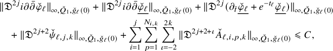 $$ \begin{align} \begin{aligned} &\|\mathfrak{D}^{2j} {i\partial\bar\partial} \check \varphi_{\ell}\|_{\infty,\check Q_{1},\check g_{\ell}(0)}+\|\mathfrak{D}^{2j} {i\partial\bar\partial} \underline{\check \varphi_{\ell}}\|_{\infty,\check Q_{1},\check g_{\ell}(0)}+\|\mathfrak{D}^{2j} (\partial_{\check t} \underline{\check \varphi_{\ell}}+e^{-t_{\ell}} \underline{\check \varphi_{\ell}} )\|_{\infty,\check Q_{1},\check g_{\ell}(0)}\\&\quad + \|\mathfrak{D}^{2j+2} \check \psi_{\ell,j,k} \|_{\infty, \check Q_{1},\check g_{\ell}(0)} +\sum_{i=1}^j \sum_{p=1}^{N_{i,k}}\sum_{\iota = -2}^{2k} \|\mathfrak{D}^{2j+2+\iota} \check A_{\ell,i,p,k}\|_{\infty, \check Q_{1},\check g_{\ell}(0)}\leqslant C, \end{aligned} \end{align} $$
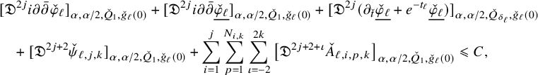 $$ \begin{align} \begin{aligned} &[\mathfrak{D}^{2j} {i\partial\bar\partial} \check \varphi_{\ell}]_{{\alpha},{\alpha}/2, \check Q_{1},\check g_{\ell}(0)}+[\mathfrak{D}^{2j} {i\partial\bar\partial} \underline{\check \varphi_{\ell}}]_{{\alpha},{\alpha}/2, \check Q_{1},\check g_{\ell}(0)}+[\mathfrak{D}^{2j} (\partial_{\check t} \underline{\check \varphi_{\ell}}+e^{-t_{\ell}} \underline{\check \varphi_{\ell}} ) ]_{{\alpha},{\alpha}/2, \check Q_{\delta_{\ell}},\check g_{\ell}(0)}\\&\quad + [\mathfrak{D}^{2j+2} \check \psi_{\ell,j,k} ]_{{\alpha},{\alpha}/2, \check Q_{1},\check g_{\ell}(0)} +\sum_{i=1}^j \sum_{p=1}^{N_{i,k}}\sum_{\iota = -2}^{2k} \left[\mathfrak{D}^{2j+2+\iota} \check A_{\ell,i,p,k}\right]_{{\alpha},{\alpha}/2, \check Q_{1},\check g_{\ell}(0)}\leqslant C, \end{aligned} \end{align} $$
where
 $\check Q_{1}$
is either
$\check Q_{1}$
is either
 $\check Q_{1}(\check z_{\ell },0)$
or
$\check Q_{1}(\check z_{\ell },0)$
or
 $\check Q_{1}(\check z_{\ell }^{\prime },\check t_{\ell }^{\prime })$
. Transferring these back to the hat picture gives
$\check Q_{1}(\check z_{\ell }^{\prime },\check t_{\ell }^{\prime })$
. Transferring these back to the hat picture gives
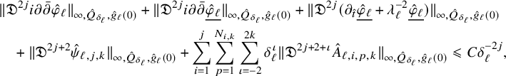 $$ \begin{align} \begin{aligned} &\|\mathfrak{D}^{2j} {i\partial\bar\partial} \hat \varphi_{\ell}\|_{\infty,\hat Q_{\delta_{\ell}},\hat g_{\ell}(0)}+\|\mathfrak{D}^{2j} {i\partial\bar\partial} \underline{\hat \varphi_{\ell}}\|_{\infty,\hat Q_{\delta_{\ell}},\hat g_{\ell}(0)}+\|\mathfrak{D}^{2j} (\partial_{\hat t} \underline{\hat \varphi_{\ell}}+\lambda_{\ell}^{-2} \underline{\hat \varphi_{\ell}} )\|_{\infty,\hat Q_{\delta_{\ell}},\hat g_{\ell}(0)}\\&\quad + \|\mathfrak{D}^{2j+2} \hat \psi_{\ell,j,k} \|_{\infty, \hat Q_{\delta_{\ell}},\hat g_{\ell}(0)} +\sum_{i=1}^j \sum_{p=1}^{N_{i,k}}\sum_{\iota = -2}^{2k} \delta_{\ell}^\iota \|\mathfrak{D}^{2j+2+\iota} \hat A_{\ell,i,p,k}\|_{\infty, \hat Q_{\delta_{\ell}},\hat g_{\ell}(0)}\leqslant C\delta_{\ell}^{-2j}, \end{aligned} \end{align} $$
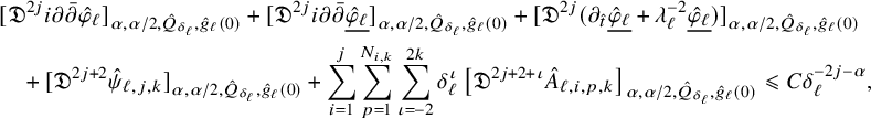 $$ \begin{align} \begin{aligned} &[\mathfrak{D}^{2j} {i\partial\bar\partial} \hat \varphi_{\ell}]_{{\alpha},{\alpha}/2, \hat Q_{\delta_{\ell}},\hat g_{\ell}(0)}+ [\mathfrak{D}^{2j} {i\partial\bar\partial} \underline{\hat \varphi_{\ell}}]_{{\alpha},{\alpha}/2, \hat Q_{\delta_{\ell}},\hat g_{\ell}(0)}+[\mathfrak{D}^{2j} (\partial_{\hat t} \underline{\hat \varphi_{\ell}}+\lambda_{\ell}^{-2} \underline{\hat \varphi_{\ell}} ) ]_{{\alpha},{\alpha}/2, \hat Q_{\delta_{\ell}},\hat g_{\ell}(0)}\\&\quad + [\mathfrak{D}^{2j+2} \hat \psi_{\ell,j,k} ]_{{\alpha},{\alpha}/2, \hat Q_{\delta_{\ell}},\hat g_{\ell}(0)} +\sum_{i=1}^j \sum_{p=1}^{N_{i,k}}\sum_{\iota = -2}^{2k} \delta_{\ell}^\iota\left[\mathfrak{D}^{2j+2+\iota} \hat A_{\ell,i,p,k}\right]_{{\alpha},{\alpha}/2, \hat Q_{\delta_{\ell}},\hat g_{\ell}(0)}\leqslant C\delta_{\ell}^{-2j-{\alpha}}, \end{aligned} \end{align} $$
where
 $\hat Q_{\delta _{\ell }}$
is either
$\hat Q_{\delta _{\ell }}$
is either
 $\hat Q_{\delta _{\ell }}(\hat z_{\ell },0)$
or
$\hat Q_{\delta _{\ell }}(\hat z_{\ell },0)$
or
 $\hat Q_{\delta _{\ell }}(\hat z_{\ell }^{\prime },\hat t_{\ell }^{\prime })$
. Using (4.95) and the triangle inequality (and the usual bound on the operator norm of
$\hat Q_{\delta _{\ell }}(\hat z_{\ell }^{\prime },\hat t_{\ell }^{\prime })$
. Using (4.95) and the triangle inequality (and the usual bound on the operator norm of
 $\mathbb {P}$
), we obtain a uniform upper bound for the numerators of (4.54) and (4.55), and so for
$\mathbb {P}$
), we obtain a uniform upper bound for the numerators of (4.54) and (4.55), and so for
 $j\geqslant 1$
, we conclude that
$j\geqslant 1$
, we conclude that
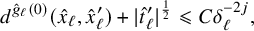 $$ \begin{align}d^{\hat g_{\ell}(0)}(\hat x_{\ell},\hat x_{\ell}^{\prime}) +|\hat t_{\ell}^{\prime}|^{\frac{1}{2}}\leqslant C\delta_{\ell}^{-2j},\end{align} $$
so that the two points
 $(\hat z_{\ell },\hat t_{\ell })$
and
$(\hat z_{\ell },\hat t_{\ell })$
and
 $(\hat z_{\ell }^{\prime },\hat t_{\ell }^{\prime })$
are approaching each other (we already know this when
$(\hat z_{\ell }^{\prime },\hat t_{\ell }^{\prime })$
are approaching each other (we already know this when
 $j=0$
thanks to (4.68)). Thus,
$j=0$
thanks to (4.68)). Thus,
 $(\hat x_{\ell }^{\prime },\hat t_{\ell }^{\prime })\in \hat Q_{\delta _{\ell }}(\hat z_{\ell },0)$
for all
$(\hat x_{\ell }^{\prime },\hat t_{\ell }^{\prime })\in \hat Q_{\delta _{\ell }}(\hat z_{\ell },0)$
for all
 $\ell $
large, and so applying (4.96) shows that the quantities in (4.54) and (4.55), which both equal
$\ell $
large, and so applying (4.96) shows that the quantities in (4.54) and (4.55), which both equal
 $1$
, are also bounded above by
$1$
, are also bounded above by
 $C\delta _{\ell }^{-2j-{\alpha }}\to 0$
, which is a contradiction.
$C\delta _{\ell }^{-2j-{\alpha }}\to 0$
, which is a contradiction.
4.7 Blowup analysis in Case 2:
$\delta _{\ell }\to \delta _\infty \in (0,+\infty )$

Without loss of generality, we can assume
 $\delta _\infty =1$
. In this case, the blowup model is
$\delta _\infty =1$
. In this case, the blowup model is
 $\mathbb {C}^m\times Y$
and
$\mathbb {C}^m\times Y$
and
 $$ \begin{align}\hat g_{\ell}^\natural(\hat t)\to g_{\mathrm{can}}|_{z=0}+g_{Y,z_\infty=0}=g_P,\end{align} $$
as
 $\ell \to +\infty $
in
$\ell \to +\infty $
in
 $C^\infty _{\mathrm {loc}}(\mathbb {C}^m\times Y\times (-\infty ,0])$
. Moreover, the complex structure also converges to a product.
$C^\infty _{\mathrm {loc}}(\mathbb {C}^m\times Y\times (-\infty ,0])$
. Moreover, the complex structure also converges to a product.
As in Case 1, Lemma 4.1 (i) implies that
 $\hat \omega _{\ell }^{\bullet }(\hat t)$
is locally uniformly equivalent to product metric on
$\hat \omega _{\ell }^{\bullet }(\hat t)$
is locally uniformly equivalent to product metric on
 $\mathbb {C}^m\times Y$
. Moreover, since
$\mathbb {C}^m\times Y$
. Moreover, since
 $\hat \omega _{\ell }^{\bullet }$
satisfies the Kähler-Ricci flow equation
$\hat \omega _{\ell }^{\bullet }$
satisfies the Kähler-Ricci flow equation
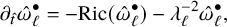 $$ \begin{align}\partial_{\hat t} \hat\omega_{\ell}^{\bullet}=-\textrm{Ric}(\hat\omega_{\ell}^{\bullet}) -\lambda_{\ell}^{-2}\hat\omega_{\ell}^{\bullet},\end{align} $$
we can again apply [Reference Chu and Lee4, Proposition 2.1] on
 $\hat Q_R(\hat z_{\ell },0)$
for R sufficiently large to obtain
$\hat Q_R(\hat z_{\ell },0)$
for R sufficiently large to obtain
 $C^\infty _{\mathrm {loc}}$
regularity of
$C^\infty _{\mathrm {loc}}$
regularity of
 $\hat \omega _{\ell }^{\bullet }$
. Arguing as in Case 1, we obtain
$\hat \omega _{\ell }^{\bullet }$
. Arguing as in Case 1, we obtain
 $C^\infty $
bounds for all the pieces in the decomposition, and using Proposition 4.4, we can assume
$C^\infty $
bounds for all the pieces in the decomposition, and using Proposition 4.4, we can assume
 $(\hat x_{\ell }^{\prime },\hat t_{\ell }^{\prime })\to (\hat x_\infty ',\hat t_\infty ')\in (\mathbb {C}^m\times Y)\times (-\infty ,0]$
. Estimating the
$(\hat x_{\ell }^{\prime },\hat t_{\ell }^{\prime })\to (\hat x_\infty ',\hat t_\infty ')\in (\mathbb {C}^m\times Y)\times (-\infty ,0]$
. Estimating the
 $C^{\alpha }$
difference quotients in (4.55) by
$C^{\alpha }$
difference quotients in (4.55) by
 $C^\beta $
ones for any
$C^\beta $
ones for any
 $\beta>\alpha $
, we see that
$\beta>\alpha $
, we see that
 $d^{\hat g_{\ell }(0)}(\hat x_{\ell },\hat x_{\ell }^{\prime })+|\hat t_{\ell }^{\prime }|^{\frac {1}{2}}\geqslant C^{-1}$
for all
$d^{\hat g_{\ell }(0)}(\hat x_{\ell },\hat x_{\ell }^{\prime })+|\hat t_{\ell }^{\prime }|^{\frac {1}{2}}\geqslant C^{-1}$
for all
 $\ell $
, which when
$\ell $
, which when
 $j=0$
is already a contradiction to (4.68).
$j=0$
is already a contradiction to (4.68).
Assuming then that
 $j\geqslant 1$
, we see that the limit
$j\geqslant 1$
, we see that the limit
 $(\hat x_\infty ,0)$
of
$(\hat x_\infty ,0)$
of
 $(\hat x_{\ell },0)$
is different from
$(\hat x_{\ell },0)$
is different from
 $(\hat x_\infty ',\hat t_\infty ')$
. By the local uniform higher order regularity, the geometric quantities smoothly subconverge as
$(\hat x_\infty ',\hat t_\infty ')$
. By the local uniform higher order regularity, the geometric quantities smoothly subconverge as
 $\ell \to +\infty $
. In particular, the limit
$\ell \to +\infty $
. In particular, the limit
 $\hat {\omega }^{\bullet }_\infty (\hat {t})$
is an ancient solution on
$\hat {\omega }^{\bullet }_\infty (\hat {t})$
is an ancient solution on
 $\mathbb {C}^m\times Y \times (-\infty ,0]$
of the Kähler-Ricci flow
$\mathbb {C}^m\times Y \times (-\infty ,0]$
of the Kähler-Ricci flow
 $$ \begin{align} \partial_{\hat t} \hat\omega_\infty^{\bullet}=-\textrm{Ric}(\hat\omega_\infty^{\bullet}). \end{align} $$
Smooth convergence also implies that (4.55) still holds in the limit.
By (4.51), we have that
 $\hat A_{\ell ,i,p,k}\to 0$
locally uniformly, hence locally smoothly, so its contributions to (4.55) vanish in the limit as
$\hat A_{\ell ,i,p,k}\to 0$
locally uniformly, hence locally smoothly, so its contributions to (4.55) vanish in the limit as
 $\ell \to +\infty $
. However, Lemma 4.1 (ii),(iii) also implies that the limits of
$\ell \to +\infty $
. However, Lemma 4.1 (ii),(iii) also implies that the limits of
 ${i\partial \bar \partial }\underline{\hat \varphi _{\ell }}$
and
${i\partial \bar \partial }\underline{\hat \varphi _{\ell }}$
and
 $\partial _{\hat t}{\hat \varphi _{\ell }}+\lambda _{\ell }^{-2}{\hat \varphi _{\ell }}$
(and hence also of
$\partial _{\hat t}{\hat \varphi _{\ell }}+\lambda _{\ell }^{-2}{\hat \varphi _{\ell }}$
(and hence also of
 $\partial _{\hat t}\underline{\hat \varphi _{\ell }}+\lambda _{\ell }^{-2}\underline{\hat \varphi _{\ell }}$
) vanish so that their contributions in (4.55) also vanish in the limit.
$\partial _{\hat t}\underline{\hat \varphi _{\ell }}+\lambda _{\ell }^{-2}\underline{\hat \varphi _{\ell }}$
) vanish so that their contributions in (4.55) also vanish in the limit.
We are left with killing the limit of the contribution of
 $\hat \psi _{\ell ,j,k}$
. For this, recall that from Lemma 4.1 (iv) we have
$\hat \psi _{\ell ,j,k}$
. For this, recall that from Lemma 4.1 (iv) we have
 $|R(g^{\bullet }(t))|\leqslant C$
, and so
$|R(g^{\bullet }(t))|\leqslant C$
, and so
 $|R(\hat {g}^{\bullet }(\hat {t}))|\leqslant C\lambda _{\ell }^{-2} \to 0$
, thus the limiting metrics
$|R(\hat {g}^{\bullet }(\hat {t}))|\leqslant C\lambda _{\ell }^{-2} \to 0$
, thus the limiting metrics
 $\hat {\omega }^{\bullet }_\infty (\hat {t})$
are scalar-flat, and hence Ricci-flat and static (using the well-known evolution equation of the scalar curvature under the Kähler-Ricci flow (4.100)). Also, since
$\hat {\omega }^{\bullet }_\infty (\hat {t})$
are scalar-flat, and hence Ricci-flat and static (using the well-known evolution equation of the scalar curvature under the Kähler-Ricci flow (4.100)). Also, since
 $\hat A_{\ell ,i,p,k}\to 0$
locally smoothly, this implies that
$\hat A_{\ell ,i,p,k}\to 0$
locally smoothly, this implies that
 $\hat {\gamma }_{\ell ,i,k}\to 0, 1\leqslant i\leqslant j,$
and so
$\hat {\gamma }_{\ell ,i,k}\to 0, 1\leqslant i\leqslant j,$
and so
 $\hat \omega _\infty ^{\bullet }=\omega _P+\hat \eta _{\infty ,j,k}$
, and in particular,
$\hat \omega _\infty ^{\bullet }=\omega _P+\hat \eta _{\infty ,j,k}$
, and in particular,
 $\hat \eta _{\infty ,j,k}$
is also static. The Liouville Theorem from [Reference Hein18] shows that
$\hat \eta _{\infty ,j,k}$
is also static. The Liouville Theorem from [Reference Hein18] shows that
 $\nabla ^{g_P}\hat \eta _{\infty ,j,k}=\nabla ^{g_P}\hat \omega _\infty ^{\bullet }\equiv 0$
. Thus
$\nabla ^{g_P}\hat \eta _{\infty ,j,k}=\nabla ^{g_P}\hat \omega _\infty ^{\bullet }\equiv 0$
. Thus
 $\hat {\eta }_{\infty ,j,k}={i\partial \bar \partial }\hat {\psi }_{\infty ,j,k}$
is parallel, with bounded
$\hat {\eta }_{\infty ,j,k}={i\partial \bar \partial }\hat {\psi }_{\infty ,j,k}$
is parallel, with bounded
 $g_P$
norm (from Lemma 4.1 (i)), so by [Reference Hein and Tosatti20, Proposition 3.12], we have
$g_P$
norm (from Lemma 4.1 (i)), so by [Reference Hein and Tosatti20, Proposition 3.12], we have
 ${i\partial \bar \partial }\hat {\psi }_{\infty ,j,k}={i\partial \bar \partial } p$
for some quadratic polynomial p on
${i\partial \bar \partial }\hat {\psi }_{\infty ,j,k}={i\partial \bar \partial } p$
for some quadratic polynomial p on
 $\mathbb {C}^m$
. This means that
$\mathbb {C}^m$
. This means that
 $\hat {\psi }_{\infty ,j,k}-p$
is pluriharmonic on
$\hat {\psi }_{\infty ,j,k}-p$
is pluriharmonic on
 $\mathbb {C}^m\times Y$
, and hence it is also pulled back from
$\mathbb {C}^m\times Y$
, and hence it is also pulled back from
 $\mathbb {C}^m$
(since Y is compact). This clearly implies that
$\mathbb {C}^m$
(since Y is compact). This clearly implies that
 $\hat {\psi }_{\infty ,j,k}$
is pulled back from
$\hat {\psi }_{\infty ,j,k}$
is pulled back from
 $\mathbb {C}^m$
, and since it also has fiberwise average zero, it must vanish identically. Thus, the contribution of
$\mathbb {C}^m$
, and since it also has fiberwise average zero, it must vanish identically. Thus, the contribution of
 $\hat \psi _{\ell ,j,k}$
to (4.55) also vanishes in the limit, and this gives a contradiction to (4.55).
$\hat \psi _{\ell ,j,k}$
to (4.55) also vanishes in the limit, and this gives a contradiction to (4.55).
4.8 Blowup analysis in Case 3:
$\delta _{\ell }\to 0$

In this case, the blowup model is
 $\mathbb {C}^m$
which is still collapsed. This is the most difficult case and will occupy most of the rest of the paper.
$\mathbb {C}^m$
which is still collapsed. This is the most difficult case and will occupy most of the rest of the paper.
By Proposition 4.4, we know that
 $(\hat x_{\ell }^{\prime },\hat t_{\ell }^{\prime })$
remains at bounded distance from
$(\hat x_{\ell }^{\prime },\hat t_{\ell }^{\prime })$
remains at bounded distance from
 $(\hat x_{\ell },0)$
. The key claim is the following non-colliding estimate, whose proof will take substantial work:
$(\hat x_{\ell },0)$
. The key claim is the following non-colliding estimate, whose proof will take substantial work:
Claim 4.5. There exists
 $\varepsilon _0>0$
such that for all
$\varepsilon _0>0$
such that for all
 $\ell \geqslant 1$
, we have
$\ell \geqslant 1$
, we have
 $$ \begin{align}d^{\hat g_{\ell}(0)}(\hat x_{\ell},\hat x_{\ell}^{\prime})+|\hat t_{\ell}^{\prime}|^{\frac{1}{2}}\geqslant \varepsilon_0>0.\end{align} $$
First, we show how to quickly complete the proof of Theorem 4.2 assuming Claim 4.5 holds. When
 $j=0$
, it is clear that (4.101) is incompatible with (4.68), while if
$j=0$
, it is clear that (4.101) is incompatible with (4.68), while if
 $j\geqslant 1$
then (4.55) implies
$j\geqslant 1$
then (4.55) implies
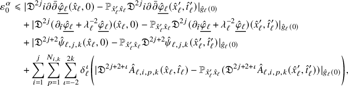 $$ \begin{align} \begin{aligned} \varepsilon_0^{\alpha} &\leqslant {|\mathfrak{D}^{2j}{i\partial\bar\partial}\underline{\hat \varphi_{\ell}}(\hat x_{\ell},0)-\mathbb{P}_{\hat x_{\ell}^{\prime}\hat x_{\ell}}\mathfrak{D}^{2j}{i\partial\bar\partial}\underline{\hat\varphi_{\ell}}(\hat x_{\ell}^{\prime},\hat t_{\ell}^{\prime})|_{\hat g_{\ell}(0)}}\\ &\quad +{|\mathfrak{D}^{2j} (\partial_{\hat t}\underline{\hat \varphi_{\ell}}+\lambda_{\ell}^{-2}\underline{\hat \varphi_{\ell}} )(\hat x_{\ell},0)-\mathbb{P}_{\hat x_{\ell}^{\prime}\hat x_{\ell}}\mathfrak{D}^{2j}(\partial_{\hat t}\underline{\hat \varphi_{\ell}}+\lambda_{\ell}^{-2}\underline{\hat \varphi_{\ell}} )(\hat x_{\ell}^{\prime},\hat t_{\ell}^{\prime})|_{\hat g_{\ell}(0)}}\\ &\quad +{|\mathfrak{D}^{2j+2} \hat \psi_{\ell,j,k}(\hat x_{\ell},0)-\mathbb{P}_{\hat x_{\ell}^{\prime}\hat x_{\ell}}\mathfrak{D}^{2j+2} \hat \psi_{\ell,j,k}(\hat x_{\ell}^{\prime},\hat t_{\ell}^{\prime})|_{\hat g_{\ell}(0)}}\\ &\quad +\sum_{i=1}^j \sum_{p=1}^{N_{i,k}}\sum_{\iota = -2}^{2k} \delta_{\ell}^\iota\Bigg({|\mathfrak{D}^{2j+2+\iota} \hat A_{\ell,i,p,k}(\hat x_{\ell},\hat t_{\ell})- \mathbb{P}_{\hat x_{\ell}^{\prime}\hat x_{\ell}}(\mathfrak{D}^{2j+2+\iota}\hat A_{\ell,i,p,k}(\hat x_{\ell}^{\prime},\hat t_{\ell}^{\prime}))|_{\hat g_{\ell}(0)}}\Bigg), \end{aligned} \end{align} $$
while the right-hand side is of
 $o(1)$
thanks to (4.77), (4.79), (4.83) and (4.87) as
$o(1)$
thanks to (4.77), (4.79), (4.83) and (4.87) as
 $\ell \to +\infty $
, since
$\ell \to +\infty $
, since
 $\delta _{\ell }\to 0$
. This is a contradiction. Therefore, to complete the proof of Theorem 4.2, it remains to prove Claim 4.5.
$\delta _{\ell }\to 0$
. This is a contradiction. Therefore, to complete the proof of Theorem 4.2, it remains to prove Claim 4.5.
4.9 Setup of secondary blowup in proving Claim 4.5
For each
 $\ell \geqslant 1$
, let
$\ell \geqslant 1$
, let
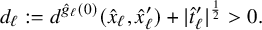 $$ \begin{align} d_{\ell}:=d^{\hat g_{\ell}(0)}(\hat x_{\ell},\hat x_{\ell}^{\prime})+|\hat t_{\ell}^{\prime}|^{\frac{1}{2}}>0. \end{align} $$
If Claim 4.5 fails to be true, then we may assume that
 $d_{\ell }\to 0$
as
$d_{\ell }\to 0$
as
 $\ell \to +\infty $
. Define a new parameter
$\ell \to +\infty $
. Define a new parameter
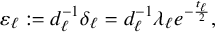 $$ \begin{align} \varepsilon_{\ell}:=d_{\ell}^{-1}\delta_{\ell}= d_{\ell}^{-1}\lambda_{\ell} e^{-\frac{t_{\ell}}{2}}, \end{align} $$
and consider the diffeomorphism
 $$ \begin{align} \Theta_{\ell}: B_{d_{\ell}^{-1}\lambda_{\ell}} \times Y\times [-d_{\ell}^{-2}\lambda_{\ell}^2t_{\ell},0] \to B_{\lambda_{\ell}}\times Y\times [-\lambda_{\ell}^2t_{\ell},0], \;\, (\hat{z},\hat{y},\hat{t}) = \Theta_{\ell}(\tilde{z},\tilde{y},\tilde{t}) =(d_{\ell}\tilde{z},\tilde{y},d_{\ell}^2\tilde{t}), \end{align} $$
As usual, we pull back time-dependent
 $2$
-tensors via
$2$
-tensors via
 $\Theta _{\ell }$
, rescale them by
$\Theta _{\ell }$
, rescale them by
 $d_{\ell }^{-2}$
and denote the new tensors with a tilde, so, for example,
$d_{\ell }^{-2}$
and denote the new tensors with a tilde, so, for example,
 $\tilde {\omega }^{\bullet }_{\ell }(\tilde {t})=d_{\ell }^{-2} \Theta _{\ell }^{*}\hat \omega _{\ell }^{\bullet }(d_{\ell }^2 \tilde {t})$
. We also apply the same pullback and rescaling procedure to the scalar functions
$\tilde {\omega }^{\bullet }_{\ell }(\tilde {t})=d_{\ell }^{-2} \Theta _{\ell }^{*}\hat \omega _{\ell }^{\bullet }(d_{\ell }^2 \tilde {t})$
. We also apply the same pullback and rescaling procedure to the scalar functions
 $\hat {A}_{\ell ,i,p,k}$
and
$\hat {A}_{\ell ,i,p,k}$
and
 $\hat {\varphi }_{\ell }$
, so
$\hat {\varphi }_{\ell }$
, so
 $\tilde A_{\ell ,i,p,k}(\tilde t)=d_{\ell }^{-2}\Theta _{\ell }^{*} \hat A_{\ell ,i,p,k}(d_{\ell }^2\tilde t), \tilde {\varphi }_{\ell }(\tilde {t})=d_{\ell }^{-2}\Theta _{\ell }^{*}\hat {\varphi }_{\ell }(d_{\ell }^2\tilde {t})$
.
$\tilde A_{\ell ,i,p,k}(\tilde t)=d_{\ell }^{-2}\Theta _{\ell }^{*} \hat A_{\ell ,i,p,k}(d_{\ell }^2\tilde t), \tilde {\varphi }_{\ell }(\tilde {t})=d_{\ell }^{-2}\Theta _{\ell }^{*}\hat {\varphi }_{\ell }(d_{\ell }^2\tilde {t})$
.
The decomposition (4.22) becomes
 $$ \begin{align} \tilde{\omega}^{\bullet}_{\ell}=\tilde{\omega}^\natural_{\ell}+\tilde{\gamma}_{\ell,0}+\tilde{\gamma}_{\ell,1,k}+\dots+\tilde{\gamma}_{\ell,j,k}+\tilde{\eta}_{\ell, j,k}, \end{align} $$
and the parabolic complex Monge-Ampère equation (4.53) becomes
 $$ \begin{align} (\tilde \omega_{\ell}^{\bullet})^{m+n}= e^{\partial_{\tilde{t}}{\tilde{\varphi}}_{\ell}+d_{\ell}^2\lambda_{\ell}^{-2}\tilde{\varphi}_{\ell}-n d_{\ell}^2\lambda_{\ell}^{-2}\tilde t} \binom{m+n}{m} \tilde \omega_{\ell,\mathrm{can}} ^m \wedge (\varepsilon_{\ell}^2 \Theta_{\ell}^{*}\Psi_{\ell}^{*} \omega_F)^n. \end{align} $$
From (4.64) (when
 $j=0$
) and (4.61) (when
$j=0$
) and (4.61) (when
 $j\geqslant 1$
), we immediately see that for any fixed
$j\geqslant 1$
), we immediately see that for any fixed
 $R>0$
and
$R>0$
and
 $\tilde t\in [-\lambda _{\ell }^2d_{\ell }^{-2}t_{\ell },0]$
, we have
$\tilde t\in [-\lambda _{\ell }^2d_{\ell }^{-2}t_{\ell },0]$
, we have
 $$ \begin{align} [{i\partial\bar\partial} \underline{\tilde \varphi_{\ell}}]_{{\alpha},{\alpha}/2,\tilde Q_{Rd_{\ell}^{-1}}(\tilde t),\tilde g_{\ell}(\tilde t)} +[{i\partial\bar\partial}\tilde{\psi}_{\ell,0,k}]_{{\alpha},{\alpha}/2,\tilde Q_{Rd_{\ell}^{-1}}(\tilde t),\tilde g_{\ell}(\tilde t)}\leqslant Cd_{\ell}^{{\alpha}}, \end{align} $$
if
 $j=0$
, and
$j=0$
, and
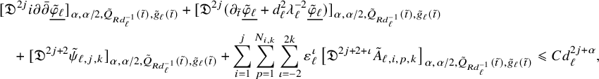 $$ \begin{align} \begin{aligned} &[\mathfrak{D}^{2j} {i\partial\bar\partial} \underline{\tilde \varphi_{\ell}}]_{{\alpha},{\alpha}/2,\tilde Q_{Rd_{\ell}^{-1}}(\tilde t),\tilde g_{\ell}(\tilde t)}+ [\mathfrak{D}^{2j} (\partial_{\tilde t}\underline{\tilde \varphi_{\ell}}+d_{\ell}^2\lambda_{\ell}^{-2}\underline{\tilde \varphi_{\ell}})]_{{\alpha},{\alpha}/2,\tilde Q_{Rd_{\ell}^{-1}}(\tilde t),\tilde g_{\ell}(\tilde t)}\\& \quad + [\mathfrak{D}^{2j+2} \tilde \psi_{\ell,j,k} ]_{{\alpha},{\alpha}/2,\tilde Q_{Rd_{\ell}^{-1}}(\tilde t),\tilde g_{\ell}(\tilde t)}+\sum_{i=1}^j \sum_{p=1}^{N_{i,k}}\sum_{\iota = -2}^{2k} \varepsilon_{\ell}^\iota\left[\mathfrak{D}^{2j+2+\iota} \tilde A_{\ell,i,p,k}\right]_{{\alpha},{\alpha}/2,\tilde Q_{Rd_{\ell}^{-1}}(\tilde t),\tilde g_{\ell}(\tilde t)}\leqslant C d_{\ell}^{2j+{\alpha}}, \end{aligned} \end{align} $$
when
 $j\geqslant 1$
, where
$j\geqslant 1$
, where
 $\tilde Q_R(\tilde t)=B_{\mathbb {C}^m}(\tilde z_{\ell },R)\times Y\times [-R^2+\tilde t,\tilde t]$
. Moreover, (4.54) and (4.55) become, respectively,
$\tilde Q_R(\tilde t)=B_{\mathbb {C}^m}(\tilde z_{\ell },R)\times Y\times [-R^2+\tilde t,\tilde t]$
. Moreover, (4.54) and (4.55) become, respectively,
 $$ \begin{align} 1=d_{\ell}^{-\alpha}\frac{|{i\partial\bar\partial} \tilde{\varphi}_{\ell}(\tilde x_{\ell},0)- \mathbb{P}_{\tilde x^{\prime}_{\ell}\tilde x_{\ell}}{i\partial\bar\partial}\tilde{\varphi}_{\ell}(\tilde x^{\prime}_{\ell},\tilde t_{\ell}^{\prime})|_{\tilde g_{\ell}(0)}}{(d^{\tilde g_{\ell}(0)}(\tilde x_{\ell},\tilde x^{\prime}_{\ell}) +|\tilde t_{\ell}^{\prime}|^{\frac{1}{2}})^{\alpha}} \end{align} $$
for
 $j=0$
and
$j=0$
and
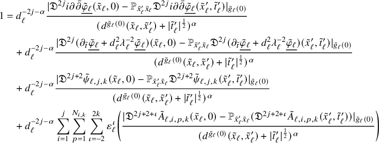 $$ \begin{align} \begin{aligned} 1&=d_{\ell}^{-2j-{\alpha}}\frac{|\mathfrak{D}^{2j} {i\partial\bar\partial} \underline{\tilde{\varphi}_{\ell}}(\tilde x_{\ell},0)- \mathbb{P}_{\tilde x^{\prime}_{\ell}\tilde x_{\ell}}\mathfrak{D}^{2j}{i\partial\bar\partial} \underline{\tilde{\varphi}_{\ell}}(\tilde x^{\prime}_{\ell},\tilde t_{\ell}^{\prime})|_{\tilde g_{\ell}(0)}}{(d^{\tilde g_{\ell}(0)}(\tilde x_{\ell},\tilde x^{\prime}_{\ell}) +|\tilde t_{\ell}^{\prime}|^{\frac{1}{2}})^{\alpha}}\\&\quad +d_{\ell}^{-2j-{\alpha}}\frac{|\mathfrak{D}^{2j} (\partial_{\tilde t}\underline{\tilde{\varphi}_{\ell}}+d_{\ell}^2\lambda_{\ell}^{-2} \underline{\tilde{\varphi}_{\ell}})(\tilde x_{\ell},0)- \mathbb{P}_{\tilde x^{\prime}_{\ell}\tilde x_{\ell}}\mathfrak{D}^{2j}(\partial_{\tilde t}\underline{\tilde{\varphi}_{\ell}}+d_{\ell}^2\lambda_{\ell}^{-2} \underline{\tilde{\varphi}_{\ell}})(\tilde x^{\prime}_{\ell},\tilde t_{\ell}^{\prime})|_{\tilde g_{\ell}(0)}}{(d^{\tilde g_{\ell}(0)}(\tilde x_{\ell},\tilde x^{\prime}_{\ell}) +|\tilde t_{\ell}^{\prime}|^{\frac{1}{2}})^{\alpha}}\\&\quad +d_{\ell}^{-2j-{\alpha}}\frac{|\mathfrak{D}^{2j+2} \tilde{\psi}_{\ell,j,k}(\tilde x_{\ell},0)- \mathbb{P}_{\tilde x^{\prime}_{\ell}\tilde x_{\ell}}\mathfrak{D}^{2j+2} \tilde{\psi}_{\ell,j,k}(\tilde x^{\prime}_{\ell},\tilde t_{\ell}^{\prime})|_{\tilde g_{\ell}(0)}}{(d^{\tilde g_{\ell}(0)}(\tilde x_{\ell},\tilde x^{\prime}_{\ell}) +|\tilde t_{\ell}^{\prime}|^{\frac{1}{2}})^{\alpha}}\\&\quad +d_{\ell}^{-2j-{\alpha}}\sum_{i=1}^j \sum_{p=1}^{N_{i,k}}\sum_{\iota = -2}^{2k} \varepsilon_{\ell}^\iota\Bigg(\frac{|\mathfrak{D}^{2j+2+\iota} \tilde A_{\ell,i,p,k}(\tilde x_{\ell},0)- \mathbb{P}_{\tilde x_{\ell}^{\prime}\tilde x_{\ell}}(\mathfrak{D}^{2j+2+\iota}\tilde A_{\ell,i,p,k}(\tilde x_{\ell}^{\prime},\tilde t_{\ell}^{\prime}))|_{\tilde g_{\ell}(0)}}{(d^{\tilde g_{\ell}(0)}(\tilde x_{\ell},\tilde x^{\prime}_{\ell}) +|\tilde t_{\ell}^{\prime}|^{\frac{1}{2}})^{\alpha}}\Bigg) \end{aligned} \end{align} $$
for
 $j\geqslant 1$
, and by definition, we also have
$j\geqslant 1$
, and by definition, we also have
 $$ \begin{align} d^{\tilde g_{\ell}(0)}(\tilde x_{\ell},\tilde x_{\ell}^{\prime})+|\tilde t^{\prime}_{\ell}|^{\frac{1}{2}}=1, \end{align} $$
for all
 $\ell>0$
.
$\ell>0$
.
For convenience, from now on,
 $\tilde Q_r$
will always denote
$\tilde Q_r$
will always denote
 $B_{\mathbb {C}^m}(0,r)\times Y\times [-r^2,0]$
, where recall that we have translated the first blowup point
$B_{\mathbb {C}^m}(0,r)\times Y\times [-r^2,0]$
, where recall that we have translated the first blowup point
 $(\tilde {x}_{\ell },\tilde {t}_{\ell })$
in the
$(\tilde {x}_{\ell },\tilde {t}_{\ell })$
in the
 $\mathbb {C}^m$
directions so that
$\mathbb {C}^m$
directions so that
 $(\tilde z_{\ell },\tilde {t}_{\ell })=(0,0)\in \mathbb {C}^m\times \mathbb {R}$
. As long as
$(\tilde z_{\ell },\tilde {t}_{\ell })=(0,0)\in \mathbb {C}^m\times \mathbb {R}$
. As long as
 $r>1$
, the cylinder
$r>1$
, the cylinder
 $\tilde {Q}_r$
always contains the other blowup point
$\tilde {Q}_r$
always contains the other blowup point
 $(\tilde {x}^{\prime }_{\ell },\tilde {t}^{\prime }_{\ell })$
because of (4.112). Following [Reference Hein and Tosatti21, §4.8], our goal is to obtain a contradiction by passing to the limit as
$(\tilde {x}^{\prime }_{\ell },\tilde {t}^{\prime }_{\ell })$
because of (4.112). Following [Reference Hein and Tosatti21, §4.8], our goal is to obtain a contradiction by passing to the limit as
 $\ell \to +\infty $
the various pieces of the decomposition, after scaling them by
$\ell \to +\infty $
the various pieces of the decomposition, after scaling them by
 $d_{\ell }^{-2j-{\alpha }}$
. To do this, we need to perform a jet subtraction centered at
$d_{\ell }^{-2j-{\alpha }}$
. To do this, we need to perform a jet subtraction centered at
 $(0,0)\in \mathbb {C}^m\times (-\infty ,0]$
for functions pulled back from the base. Given
$(0,0)\in \mathbb {C}^m\times (-\infty ,0]$
for functions pulled back from the base. Given
 $r\in \mathbb {N}$
, the parabolic r-jet at
$r\in \mathbb {N}$
, the parabolic r-jet at
 $(0,0)$
of a function u in
$(0,0)$
of a function u in
 $\mathbb {C}^m\times (-\infty ,0]$
is given by
$\mathbb {C}^m\times (-\infty ,0]$
is given by
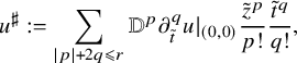 $$ \begin{align} u^\sharp:=\sum_{|p|+2q\leqslant r} {\mathbb{D}}^p\partial_{\tilde{t}}^q u |_{(0,0)} \frac{\tilde{z}^p}{p!}\frac{{\tilde{t}}^q}{q!}, \end{align} $$
using standard multiindex notation, where here we treat
 $\tilde {z}$
as real variables. The parabolic degree of such a polynomial is defined by letting the
$\tilde {z}$
as real variables. The parabolic degree of such a polynomial is defined by letting the
 $\tilde {z}$
variables have degree
$\tilde {z}$
variables have degree
 $1$
and the
$1$
and the
 ${\tilde {t}}$
variable degree
${\tilde {t}}$
variable degree
 $2$
. Thus, the degree of
$2$
. Thus, the degree of
 $u^\sharp $
is at most r. We will also write
$u^\sharp $
is at most r. We will also write
 $u^{*}:=u-u^\sharp $
, whose r-jet at
$u^{*}:=u-u^\sharp $
, whose r-jet at
 $(0,0)$
thus vanishes.
$(0,0)$
thus vanishes.
With this notation, we define
 $\tilde A_{\ell ,i,p,k}^\sharp $
as the parabolic
$\tilde A_{\ell ,i,p,k}^\sharp $
as the parabolic
 $2j$
-jet of
$2j$
-jet of
 $\tilde A_{\ell ,i,p,k}$
at
$\tilde A_{\ell ,i,p,k}$
at
 $(0,0)$
, and define
$(0,0)$
, and define
 $\tilde A_{\ell ,i,p,k}^{*}=\tilde A_{\ell ,i,p,k}-\tilde A_{\ell ,i,p,k}^\sharp $
so that
$\tilde A_{\ell ,i,p,k}^{*}=\tilde A_{\ell ,i,p,k}-\tilde A_{\ell ,i,p,k}^\sharp $
so that
 ${\mathbb {D}}^{p} \partial _{\tilde {t}}^q \tilde A_{\ell ,i,p,k}^{*}|_{(0,0)}=0$
for any
${\mathbb {D}}^{p} \partial _{\tilde {t}}^q \tilde A_{\ell ,i,p,k}^{*}|_{(0,0)}=0$
for any
 $p+2q\leqslant 2j$
. As for the potential
$p+2q\leqslant 2j$
. As for the potential
 $\underline{\tilde {\varphi }_{\ell }}$
, since the PDE (4.107) and the blowup quantity in (4.109) (for
$\underline{\tilde {\varphi }_{\ell }}$
, since the PDE (4.107) and the blowup quantity in (4.109) (for
 $j\geqslant 1$
) both contain the term
$j\geqslant 1$
) both contain the term
 $\partial _{\tilde {t}}{\tilde {\varphi }}_{\ell }+d_{\ell }^2\lambda _{\ell }^{-2}\tilde {\varphi }_{\ell }$
, it will be more convenient to consider instead
$\partial _{\tilde {t}}{\tilde {\varphi }}_{\ell }+d_{\ell }^2\lambda _{\ell }^{-2}\tilde {\varphi }_{\ell }$
, it will be more convenient to consider instead
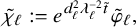 $$ \begin{align} \tilde{\chi}_{\ell}:=e^{d_{\ell}^2\lambda_{\ell}^{-2}\tilde t} {\tilde{\varphi}_{\ell}}, \end{align} $$
so that
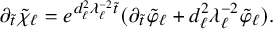 $$ \begin{align} \partial_{\tilde{t}}\tilde{\chi}_{\ell}=e^{d_{\ell}^2\lambda_{\ell}^{-2}\tilde t}(\partial_{\tilde{t}}{\tilde{\varphi}}_{\ell}+d_{\ell}^2\lambda_{\ell}^{-2}\tilde{\varphi}_{\ell}). \end{align} $$
We claim that the fiber average
 $\underline{\tilde {\chi }_{\ell }}$
satisfies estimates similar to those satisfied by
$\underline{\tilde {\chi }_{\ell }}$
satisfies estimates similar to those satisfied by
 $ \underline{\tilde {\varphi }_{\ell }}$
in (4.108) and (4.109):
$ \underline{\tilde {\varphi }_{\ell }}$
in (4.108) and (4.109):
Claim 4.6. For any fixed
 $R>0$
, we have
$R>0$
, we have
 $$ \begin{align} d_{\ell}^{-2j-{\alpha}}\left|[\mathfrak{D}^{2j} \partial_{\tilde t}\underline{\tilde \chi_{\ell}}]_{{\alpha},{\alpha}/2,\tilde Q_{Rd_{\ell}^{-1}},\tilde g_{\ell}(0)}- [\mathfrak{D}^{2j} \left( \partial_{\tilde t}\underline{\tilde{\varphi}_{\ell}}+d_{\ell}^2\lambda_{\ell}^{-2}\underline{\tilde{\varphi}_{\ell}} \right) ]_{{\alpha},{\alpha}/2,\tilde Q_{Rd_{\ell}^{-1}},\tilde g_{\ell}(0)}\right|&=o(1), \end{align} $$
 $$ \begin{align} d_{\ell}^{-2j-{\alpha}}\left|[\mathfrak{D}^{2j} {i\partial\bar\partial} \underline{ \tilde \chi_{\ell}}]_{{\alpha},{\alpha}/2,\tilde Q_{Rd_{\ell}^{-1}},\tilde g_{\ell}(0)}-[\mathfrak{D}^{2j} {i\partial\bar\partial} \underline{ \tilde \varphi _{\ell}}]_{{\alpha},{\alpha}/2,\tilde Q_{Rd_{\ell}^{-1}},\tilde g_{\ell}(0)}\right|&=o(1), \end{align} $$
as
 $\ell \to +\infty $
.
$\ell \to +\infty $
.
Proof of Claim 4.6
We first treat
 $\partial _{\tilde t}\underline{\tilde {\chi }_{\ell }}$
, and since this will only be used when
$\partial _{\tilde t}\underline{\tilde {\chi }_{\ell }}$
, and since this will only be used when
 $j\geqslant 1$
, we only prove it here in this case (but see (4.137) and (4.147) below for a stronger statement when
$j\geqslant 1$
, we only prove it here in this case (but see (4.137) and (4.147) below for a stronger statement when
 $j=0$
). Observe first that for any
$j=0$
). Observe first that for any
 $r\in \mathbb {N}$
, we have
$r\in \mathbb {N}$
, we have
 $$ \begin{align} \left\|\partial_{\tilde{t}}^r \left(e^{d_{\ell}^2\lambda_{\ell}^{-2}\tilde t}\right)\right\|_{\infty,\tilde Q_{Rd_{\ell}^{-1}}}=(1+o(1))(d_{\ell}\lambda_{\ell}^{-1})^{2r}. \end{align} $$
Using this, we bound
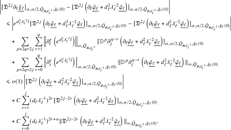 $$ \begin{align} \begin{aligned} &\left|[\mathfrak{D}^{2j} \partial_{\tilde t}\underline{\tilde \chi_{\ell}}]_{{\alpha},{\alpha}/2,\tilde Q_{Rd_{\ell}^{-1}},\tilde g_{\ell}(0)}- [\mathfrak{D}^{2j} \left( \partial_{\tilde t}\underline{\tilde{\varphi}_{\ell}}+d_{\ell}^2\lambda_{\ell}^{-2}\underline{\tilde{\varphi}_{\ell}} \right) ]_{{\alpha},{\alpha}/2,\tilde Q_{Rd_{\ell}^{-1}},\tilde g_{\ell}(0)}\right|\\&\quad \leqslant \left|e^{d_{\ell}^2\lambda_{\ell}^{-2}\tilde t}[\mathfrak{D}^{2j} \left( \partial_{\tilde t}\underline{\tilde{\varphi}_{\ell}}+d_{\ell}^2\lambda_{\ell}^{-2}\underline{\tilde{\varphi}_{\ell}} \right) ]_{{\alpha},{\alpha}/2,\tilde Q_{Rd_{\ell}^{-1}},\tilde g_{\ell}(0)}- [\mathfrak{D}^{2j} \left( \partial_{\tilde t}\underline{\tilde{\varphi}_{\ell}}+d_{\ell}^2\lambda_{\ell}^{-2}\underline{\tilde{\varphi}_{\ell}} \right) ]_{{\alpha},{\alpha}/2,\tilde Q_{Rd_{\ell}^{-1}},\tilde g_{\ell}(0)}\right|\\&\qquad +\sum_{p+2q=2j}\sum_{r=1}^q \left\|\partial_{\tilde{t}}^r \left(e^{d_{\ell}^2\lambda_{\ell}^{-2}\tilde t}\right)\right\|_{\infty,\tilde Q_{Rd_{\ell}^{-1}}} [{\mathbb{D}}^p\partial_{\tilde t}^{q-r} \left( \partial_{\tilde t}\underline{\tilde{\varphi}_{\ell}}+d_{\ell}^2\lambda_{\ell}^{-2}\underline{\tilde{\varphi}_{\ell}} \right) ]_{{\alpha},{\alpha}/2,\tilde Q_{Rd_{\ell}^{-1}},\tilde g_{\ell}(0)}\\&\qquad + \sum_{p+2q=2j}\sum_{r=0}^q \left[\partial_{\tilde{t}}^r \left(e^{d_{\ell}^2\lambda_{\ell}^{-2}\tilde t}\right)\right]_{{\alpha},{\alpha}/2,\tilde Q_{Rd_{\ell}^{-1}},\tilde g_{\ell}(0)} \|{\mathbb{D}}^p\partial_{\tilde t}^{q-r} \left( \partial_{\tilde t}\underline{\tilde{\varphi}_{\ell}}+d_{\ell}^2\lambda_{\ell}^{-2}\underline{\tilde{\varphi}_{\ell}} \right) \|_{\infty,\tilde Q_{Rd_{\ell}^{-1}},\tilde g_{\ell}(0)}\\&\quad \leqslant o(1)\left|[\mathfrak{D}^{2j} \left( \partial_{\tilde t}\underline{\tilde{\varphi}_{\ell}}+d_{\ell}^2\lambda_{\ell}^{-2}\underline{\tilde{\varphi}_{\ell}} \right) ]_{{\alpha},{\alpha}/2,\tilde Q_{Rd_{\ell}^{-1}},\tilde g_{\ell}(0)}\right|\\&\qquad +C\sum_{r=1}^j (d_{\ell}\lambda_{\ell}^{-1})^{2r} [\mathfrak{D}^{2j-2r} \left( \partial_{\tilde t}\underline{\tilde{\varphi}_{\ell}}+d_{\ell}^2\lambda_{\ell}^{-2}\underline{\tilde{\varphi}_{\ell}} \right) ]_{{\alpha},{\alpha}/2,\tilde Q_{Rd_{\ell}^{-1}},\tilde g_{\ell}(0)}\\&\qquad + C\sum_{r=0}^j (d_{\ell}\lambda_{\ell}^{-1} )^{2r+{\alpha}} \|\mathfrak{D}^{2j-2r} \left( \partial_{\tilde t}\underline{\tilde{\varphi}_{\ell}}+d_{\ell}^2\lambda_{\ell}^{-2}\underline{\tilde{\varphi}_{\ell}} \right) \|_{\infty,\tilde Q_{Rd_{\ell}^{-1}},\tilde g_{\ell}(0)}. \end{aligned} \end{align} $$
Thanks to (4.109), the third line from the bottom is
 $o(d_{\ell }^{2j+{\alpha }})$
. As for the last two lines, we interpolate between (4.109) and the estimate
$o(d_{\ell }^{2j+{\alpha }})$
. As for the last two lines, we interpolate between (4.109) and the estimate
 $\| \partial _{\tilde t}\underline{\tilde {\varphi }_{\ell }}+d_{\ell }^2\lambda _{\ell }^{-2}\underline{\tilde {\varphi }_{\ell }} \|_{\infty ,\tilde Q_{Rd_{\ell }^{-1}}}=o(1)$
which comes from Lemma 4.1 (ii), and we get for each
$\| \partial _{\tilde t}\underline{\tilde {\varphi }_{\ell }}+d_{\ell }^2\lambda _{\ell }^{-2}\underline{\tilde {\varphi }_{\ell }} \|_{\infty ,\tilde Q_{Rd_{\ell }^{-1}}}=o(1)$
which comes from Lemma 4.1 (ii), and we get for each
 $1\leqslant \iota \leqslant 2j$
,
$1\leqslant \iota \leqslant 2j$
,
 $$ \begin{align} \begin{aligned} &\quad d_{\ell}^{-\iota}(R-\rho)^{\iota} \|\mathfrak{D}^{\iota} \left( \partial_{\tilde t}\underline{\tilde{\varphi}_{\ell}}+d_{\ell}^2\lambda_{\ell}^{-2}\underline{\tilde{\varphi}_{\ell}} \right) \|_{\infty,\tilde Q_{\rho d_{\ell}^{-1}},\tilde g_{\ell}(0)}\leqslant C(R-\rho)^{2j+{\alpha}} +o(1). \end{aligned} \end{align} $$
By choosing
 $R-\rho \approx 1$
(which is clearly allowed) and replacing R by a slightly smaller one, we see that for all
$R-\rho \approx 1$
(which is clearly allowed) and replacing R by a slightly smaller one, we see that for all
 $1\leqslant \iota \leqslant 2j$
,
$1\leqslant \iota \leqslant 2j$
,
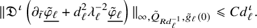 $$ \begin{align} \|\mathfrak{D}^{\iota} \left( \partial_{\tilde t}\underline{\tilde{\varphi}_{\ell}}+d_{\ell}^2\lambda_{\ell}^{-2}\underline{\tilde{\varphi}_{\ell}} \right) \|_{\infty,\tilde Q_{R d_{\ell}^{-1}},\tilde g_{\ell}(0)}\leqslant C d_{\ell}^{\iota}. \end{align} $$
We can then estimate
 $$ \begin{align} \begin{aligned} &\sum_{r=0}^j (d_{\ell}\lambda_{\ell}^{-1} )^{2r+{\alpha}} \|\mathfrak{D}^{2j-2r} \left( \partial_{\tilde t}\underline{\tilde{\varphi}_{\ell}}+d_{\ell}^2\lambda_{\ell}^{-2}\underline{\tilde{\varphi}_{\ell}} \right) \|_{\infty,\tilde Q_{Rd_{\ell}^{-1}},\tilde g_{\ell}(0)}\\& \quad \leqslant C\sum_{r=0}^j (d_{\ell}\lambda_{\ell}^{-1} )^{2r+{\alpha}} d_{\ell}^{2j-2r}=C \lambda_{\ell}^{-{\alpha}} d_{\ell}^{2j+{\alpha}}=o(d_{\ell}^{2j+{\alpha}}), \end{aligned} \end{align} $$
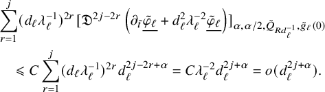 $$ \begin{align} \begin{aligned} &\sum_{r=1}^j (d_{\ell}\lambda_{\ell}^{-1})^{2r} [\mathfrak{D}^{2j-2r} \left( \partial_{\tilde t}\underline{\tilde{\varphi}_{\ell}}+d_{\ell}^2\lambda_{\ell}^{-2}\underline{\tilde{\varphi}_{\ell}} \right) ]_{{\alpha},{\alpha}/2,\tilde Q_{Rd_{\ell}^{-1}},\tilde g_{\ell}(0)}\\& \quad\leqslant C \sum_{r=1}^j (d_{\ell}\lambda_{\ell}^{-1})^{2r} d_{\ell}^{2j-2r+{\alpha}}= C\lambda_{\ell}^{-2} d_{\ell}^{2j+{\alpha}}=o(d_{\ell}^{2j+{\alpha}}). \end{aligned} \end{align} $$
Putting these together proves (4.116).
Next, we treat
 ${i\partial \bar \partial }\underline{ \tilde {\chi }_{\ell }}$
in a similar fashion (allowing now also
${i\partial \bar \partial }\underline{ \tilde {\chi }_{\ell }}$
in a similar fashion (allowing now also
 $j=0$
),
$j=0$
),
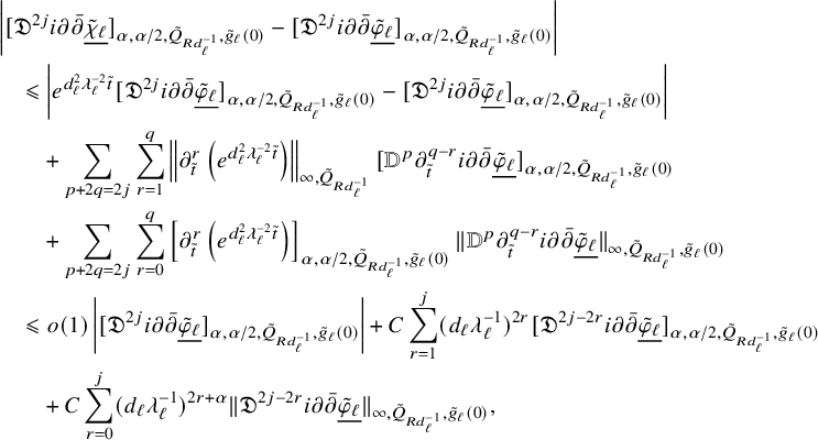 $$ \begin{align} \begin{aligned} &\left| [\mathfrak{D}^{2j} {i\partial\bar\partial} \underline{\tilde{\chi}_{\ell}}]_{{\alpha},{\alpha}/2,\tilde Q_{Rd_{\ell}^{-1}},\tilde g_{\ell}(0)} -[\mathfrak{D}^{2j}{i\partial\bar\partial}\underline{\tilde{\varphi} _{\ell}}]_{{\alpha},{\alpha}/2,\tilde Q_{Rd_{\ell}^{-1}},\tilde g_{\ell}(0)}\right|\\& \quad \leqslant \left|e^{d_{\ell}^2\lambda_{\ell}^{-2}\tilde t}[\mathfrak{D}^{2j} {i\partial\bar\partial} \underline{\tilde{\varphi} _{\ell}}]_{{\alpha},{\alpha}/2,\tilde Q_{Rd_{\ell}^{-1}},\tilde g_{\ell}(0)} -[\mathfrak{D}^{2j}{i\partial\bar\partial}\underline{\tilde{\varphi} _{\ell}}]_{{\alpha},{\alpha}/2,\tilde Q_{Rd_{\ell}^{-1}},\tilde g_{\ell}(0)}\right|\\&\qquad +\sum_{p+2q=2j}\sum_{r=1}^q \left\|\partial_{\tilde{t}}^r \left(e^{d_{\ell}^2\lambda_{\ell}^{-2}\tilde t}\right)\right\|_{\infty,\tilde Q_{Rd_{\ell}^{-1}}} [{\mathbb{D}}^p\partial_{\tilde t}^{q-r} {i\partial\bar\partial} \underline{\tilde{\varphi}_{\ell}}]_{{\alpha},{\alpha}/2,\tilde Q_{Rd_{\ell}^{-1}},\tilde g_{\ell}(0)}\\&\qquad +\sum_{p+2q=2j}\sum_{r=0}^q \left[\partial_{\tilde{t}}^r \left(e^{d_{\ell}^2\lambda_{\ell}^{-2}\tilde t}\right)\right]_{{\alpha},{\alpha}/2,\tilde Q_{Rd_{\ell}^{-1}},\tilde g_{\ell}(0)} \|{\mathbb{D}}^p\partial_{\tilde t}^{q-r} {i\partial\bar\partial} \underline{\tilde{\varphi}_{\ell}}\|_{\infty,\tilde Q_{Rd_{\ell}^{-1}},\tilde g_{\ell}(0)}\\&\quad \leqslant o(1)\left|[\mathfrak{D}^{2j}{i\partial\bar\partial}\underline{\tilde{\varphi} _{\ell}}]_{{\alpha},{\alpha}/2,\tilde Q_{Rd_{\ell}^{-1}},\tilde g_{\ell}(0)}\right| +C\sum_{r=1}^j (d_{\ell}\lambda_{\ell}^{-1})^{2r} [\mathfrak{D}^{2j-2r} {i\partial\bar\partial} \underline{\tilde{\varphi}_{\ell}}]_{{\alpha},{\alpha}/2,\tilde Q_{Rd_{\ell}^{-1}},\tilde g_{\ell}(0)}\\&\qquad +C\sum_{r=0}^j (d_{\ell}\lambda_{\ell}^{-1} )^{2r+{\alpha}} \|\mathfrak{D}^{2j-2r} {i\partial\bar\partial} \underline{\tilde{\varphi}_{\ell}}\|_{\infty,\tilde Q_{Rd_{\ell}^{-1}},\tilde g_{\ell}(0)}, \end{aligned} \end{align} $$
and then we continue the argument exactly as above, using the bound (4.108) when
 $j=0$
. This proves (4.117).
$j=0$
. This proves (4.117).
With this modification in mind, we let
 $\underline{ \tilde \chi _{\ell }^\sharp }$
be the (parabolic) jet of
$\underline{ \tilde \chi _{\ell }^\sharp }$
be the (parabolic) jet of
 $\underline{ \tilde \chi _{\ell }}=e^{d_{\ell }^2\lambda _{\ell }^{-2}\tilde t}\underline{\tilde {\varphi }_{\ell }}$
at
$\underline{ \tilde \chi _{\ell }}=e^{d_{\ell }^2\lambda _{\ell }^{-2}\tilde t}\underline{\tilde {\varphi }_{\ell }}$
at
 $(\tilde z,\tilde t)=(0,0)$
of order
$(\tilde z,\tilde t)=(0,0)$
of order
 $2j+2$
, and define
$2j+2$
, and define
 $\underline{\tilde {\chi }_{\ell }^{*}}:=\underline{ \tilde {\chi }_{\ell }}-\underline{ \tilde {\chi }_{\ell }^\sharp }$
. Define also
$\underline{\tilde {\chi }_{\ell }^{*}}:=\underline{ \tilde {\chi }_{\ell }}-\underline{ \tilde {\chi }_{\ell }^\sharp }$
. Define also
 $$ \begin{align} \tilde{\eta}_{\ell}^\ddagger:=e^{-d_{\ell}^2\lambda_{\ell}^{-2}\tilde t}{i\partial\bar\partial} \underline{\tilde{\chi}_{\ell}^\sharp},\quad\quad \tilde{\eta}_{\ell}^\diamondsuit:=e^{-d_{\ell}^2\lambda_{\ell}^{-2}\tilde t}{i\partial\bar\partial} \underline{ \tilde{\chi}_{\ell}^{*}}, \end{align} $$
so that by definition, we have
 $$ \begin{align} {i\partial\bar\partial}\underline{\tilde{\varphi }_{\ell}}=\tilde{\eta}_{\ell}^\ddagger+\tilde{\eta}_{\ell}^\diamondsuit. \end{align} $$
Recall that for
 $1\leqslant i\leqslant j$
, we had defined
$1\leqslant i\leqslant j$
, we had defined
 $$ \begin{align} \tilde \gamma_{\ell,i,k}=\sum_{p=1}^{N_{i,k}} {i\partial\bar\partial} \tilde{\mathfrak{G}}_{\tilde{t},k}(\tilde A_{\ell,i,p,k},\tilde G_{\ell,i,p,k} ) \end{align} $$
(see also (4.347) below for an explicit formula). We shall further denote
 $$ \begin{align} \tilde{\eta}_{\ell}^\circ :=\sum_{i=1}^j \sum_{p=1}^{N_{i,k}}{i\partial\bar\partial} \tilde{\mathfrak{G}}_{\tilde{t},k}(\tilde A_{\ell,i,p,k}^{*},\tilde G_{\ell,i,p,k}),\quad \tilde{\eta}_{\ell}^\dagger :=\sum_{i=1}^j \sum_{p=1}^{N_{i,k}}{i\partial\bar\partial} \tilde{\mathfrak{G}}_{\tilde{t},k}(\tilde A_{\ell,i,p,k}^\sharp,\tilde G_{\ell,i,p,k}), \end{align} $$
so that
 $$ \begin{align} \begin{aligned} \tilde{\omega}_{\ell}^{\bullet}&=\tilde \omega_{\ell}^\natural +{i\partial\bar\partial} \underline{ \tilde{\varphi}_{\ell}}+\sum_{i=1}^j\sum_{p=1}^{N_{i,k}}{i\partial\bar\partial} \tilde{\mathfrak{G}}_{\tilde{t},k}(\tilde A_{\ell,i,p,k},\tilde G_{\ell,i,p,k})+{i\partial\bar\partial} \tilde{\psi}_{\ell,j,k}\\ &=\tilde \omega_{\ell}^\natural +\tilde{\eta}_{\ell}^\dagger+\tilde{\eta}_{\ell}^\ddagger+\tilde{\eta}_{\ell}^\circ+\tilde{\eta}_{\ell}^\diamondsuit+\tilde{\eta}_{\ell,j,k}, \end{aligned} \end{align} $$
and we will write
 $\tilde {\omega }_{\ell }^\sharp :=\tilde \omega _{\ell }^\natural +\tilde {\eta }_{\ell }^\dagger +\tilde {\eta }_{\ell }^\ddagger $
.
$\tilde {\omega }_{\ell }^\sharp :=\tilde \omega _{\ell }^\natural +\tilde {\eta }_{\ell }^\dagger +\tilde {\eta }_{\ell }^\ddagger $
.
Thanks to these jet subtractions, and to Claim 4.6, from (4.108), (4.109), (4.111) and (4.112), we obtain
 $$ \begin{align} [{i\partial\bar\partial}\underline{\tilde{\chi}_{\ell}^{*}}]_{{\alpha},{\alpha}/2,\tilde Q_{Rd_{\ell}^{-1}},\tilde g_{\ell}(0)}+[{i\partial\bar\partial}\tilde \psi_{\ell,0,k} ]_{{\alpha},{\alpha}/2,\tilde Q_{Rd_{\ell}^{-1}},\tilde g_{\ell}(0)} \leqslant C d_{\ell}^{{\alpha}} \end{align} $$
when
 $j=0$
, and
$j=0$
, and
 $$ \begin{align} \begin{aligned} &[\mathfrak{D}^{2j} {i\partial\bar\partial}\underline{\tilde{\chi}_{\ell}^{*}}]_{{\alpha},{\alpha}/2,\tilde Q_{Rd_{\ell}^{-1}},\tilde g_{\ell}(0)}+ [\mathfrak{D}^{2j} \partial_{\tilde t}\underline{\tilde{\chi}_{\ell}^{*}}]_{{\alpha},{\alpha}/2,\tilde Q_{Rd_{\ell}^{-1}},\tilde g_{\ell}(0)}\\& \quad + [\mathfrak{D}^{2j+2} \tilde \psi_{\ell,j,k} ]_{{\alpha},{\alpha}/2,\tilde Q_{Rd_{\ell}^{-1}},\tilde g_{\ell}(0)} +\sum_{i=1}^j \sum_{p=1}^{N_{i,k}}\sum_{\iota = -2}^{2k} \varepsilon_{\ell}^\iota\left[\mathfrak{D}^{2j+2+\iota} \tilde A^{*}_{\ell,i,p,k}\right]_{{\alpha},{\alpha}/2,\tilde Q_{Rd_{\ell}^{-1}},\tilde g_{\ell}( 0)}\leqslant C d_{\ell}^{2j+{\alpha}}, \end{aligned} \end{align} $$
when
 $j\geqslant 1$
, as well as
$j\geqslant 1$
, as well as
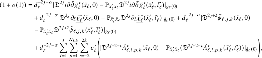 $$ \begin{align} \begin{aligned} (1+o(1))&=d_{\ell}^{-2j-{\alpha}}|\mathfrak{D}^{2j} {i\partial\bar\partial} \underline{\tilde{\chi}_{\ell}^{*}}(\tilde x_{\ell},0)- \mathbb{P}_{\tilde x^{\prime}_{\ell}\tilde x_{\ell}}\mathfrak{D}^{2j} {i\partial\bar\partial} \underline{\tilde{\chi}_{\ell}^{*}}(\tilde x^{\prime}_{\ell},\tilde t_{\ell}^{\prime})|_{\tilde g_{\ell}(0)}\\& \quad +d_{\ell}^{-2j-{\alpha}}|\mathfrak{D}^{2j} \partial_{\tilde t} \underline{\tilde{\chi}_{\ell}^{*}}(\tilde x_{\ell},0)- \mathbb{P}_{\tilde x^{\prime}_{\ell}\tilde x_{\ell}}\mathfrak{D}^{2j} \partial_{\tilde t} \underline{\tilde{\chi}_{\ell}^{*}}(\tilde x^{\prime}_{\ell},\tilde t_{\ell}^{\prime})|_{\tilde g_{\ell}(0)}+d_{\ell}^{-2j-{\alpha}}|\mathfrak{D}^{2j+2} \tilde \psi_{\ell,j,k}(\tilde x_{\ell},0)\\& \quad - \mathbb{P}_{\tilde x^{\prime}_{\ell}\tilde x_{\ell}}\mathfrak{D}^{2j+2} \tilde{\psi}_{\ell,j,k}(\tilde x^{\prime}_{\ell},\tilde t_{\ell}^{\prime})|_{\tilde g_{\ell}(0)}\\& \quad +d_{\ell}^{-2j-{\alpha}}\sum_{i=1}^j \sum_{p=1}^{N_{i,k}}\sum_{\iota = -2}^{2k} \varepsilon_{\ell}^\iota\Bigg({|\mathfrak{D}^{2j+2+\iota} \tilde A^{*}_{\ell,i,p,k}(\tilde x_{\ell},0)- \mathbb{P}_{\tilde x_{\ell}^{\prime}\tilde x_{\ell}}(\mathfrak{D}^{2j+2+\iota}\tilde A^{*}_{\ell,i,p,k}(\tilde x_{\ell}^{\prime},\tilde t_{\ell}^{\prime}))|_{\tilde g_{\ell}(0)}}\Bigg), \end{aligned} \end{align} $$
while on the other hand (4.110), remains the same for
 $j=0$
.
$j=0$
.
4.10 Estimates on each component
Our next task is then to obtain precise estimates on all the pieces of the decomposition (4.129), which will allow us to later expand and linearize the Monge-Ampère equation (4.107). In the following, the radii R and S will be any fixed radii, unless otherwise specified. Some of the estimates are analogous to those in [Reference Hein and Tosatti21, §4.9], replacing balls
 $\tilde {B}_r$
by parabolic cylinders
$\tilde {B}_r$
by parabolic cylinders
 $\tilde {Q}_r=B_{\mathbb {C}^m}(0,r)\times Y\times [-r^2,0]$
. We follow closely the arguments there.
$\tilde {Q}_r=B_{\mathbb {C}^m}(0,r)\times Y\times [-r^2,0]$
. We follow closely the arguments there.
4.10.1 Estimates for
$\tilde {\psi }_{\ell ,j,k}$

First, we assume that
 $j=0$
. Then from the Hölder seminorm bound for
$j=0$
. Then from the Hölder seminorm bound for
 ${i\partial \bar \partial }\hat {\psi }_{\ell ,0,k}$
in (4.64), together with Proposition 2.6, we obtain
${i\partial \bar \partial }\hat {\psi }_{\ell ,0,k}$
in (4.64), together with Proposition 2.6, we obtain
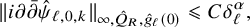 $$ \begin{align} \| {i\partial\bar\partial}\hat\psi_{\ell,0,k} \|_{\infty,\hat{Q}_{R},\hat g_{\ell}(0)}\leqslant C \delta_{\ell}^{{\alpha}}, \end{align} $$
and since
 $\hat {\psi }_{\ell ,0,k}$
has fiberwise average zero, we can apply fiberwise Moser iteration to this, and get
$\hat {\psi }_{\ell ,0,k}$
has fiberwise average zero, we can apply fiberwise Moser iteration to this, and get
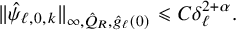 $$ \begin{align} \|\hat\psi_{\ell,0,k} \|_{\infty,\hat{Q}_{R},\hat g_{\ell}(0)}\leqslant C \delta_{\ell}^{2+{\alpha}}. \end{align} $$
Using the bounds
 $\|\partial _{t}^2\varphi +\partial _{t}\varphi \|_{\infty , B\times Y\times [t-1,t]}\leqslant C$
and
$\|\partial _{t}^2\varphi +\partial _{t}\varphi \|_{\infty , B\times Y\times [t-1,t]}\leqslant C$
and
 $\|{\mathbb {D}}(\partial _{t}\varphi +\varphi )\|_{\infty , B\times Y\times [t-1,t],g(t)}\leqslant C$
from Lemma 4.1 (v), (vi), we can bound for any
$\|{\mathbb {D}}(\partial _{t}\varphi +\varphi )\|_{\infty , B\times Y\times [t-1,t],g(t)}\leqslant C$
from Lemma 4.1 (v), (vi), we can bound for any
 $x,x'\in B_{R\lambda _{\ell }^{-1}}\times Y$
and
$x,x'\in B_{R\lambda _{\ell }^{-1}}\times Y$
and
 $t,s\in (t_{\ell }-\lambda _{\ell }^{-2}R^2,t_{\ell }]$
,
$t,s\in (t_{\ell }-\lambda _{\ell }^{-2}R^2,t_{\ell }]$
,
 $$ \begin{align} |(\partial_{t}\varphi +\varphi )(x,t)-(\partial_{t}\varphi +\varphi )(x',s)|\leqslant C(d^{g(t)}(x,x')+|t-s|)\leqslant o(1) (d^{g(t)}(x,x')+|t-s|^{\frac{1}{2}})^{\alpha}, \end{align} $$
which gives
 $$ \begin{align} [\partial_{\hat{t}}\hat{\varphi }_{\ell}+\lambda_{\ell}^{-2}\hat{\varphi }_{\ell}]_{{\alpha},{\alpha}/2,\hat{Q}_R,\hat{g}_{\ell}(0)}\leqslant \lambda_{\ell}^{-\alpha}[\partial_{t}\varphi +\varphi ]_{{\alpha},{\alpha}/2,B_{R \lambda_{\ell}^{-1}}\times Y\times(t_{\ell}-\lambda_{\ell}^{-2}R^2,t_{\ell}],g(t_{\ell})}=o(1). \end{align} $$
Repeating the argument with
 $\underline{\varphi }$
gives
$\underline{\varphi }$
gives
 $$ \begin{align} [\partial_{\hat{t}}\underline{\hat{\varphi }_{\ell}}+\lambda_{\ell}^{-2}\underline{\hat{\varphi }_{\ell}}]_{{\alpha},{\alpha}/2,\hat{Q}_R,\hat{g}_{\ell}(0)}=o(1), \end{align} $$
and combining these, we see that
 $$ \begin{align} [\partial_{\hat{t}}\hat{\psi}_{\ell,0,k}+\lambda_{\ell}^{-2}\hat{\psi}_{\ell,0,k}]_{{\alpha},{\alpha}/2,\hat{Q}_R,\hat{g}_{\ell}(0)}=o(1), \end{align} $$
so from this, the bound
 $[{i\partial \bar \partial }\hat {\psi }_{\ell ,0,k}]_{{\alpha },{\alpha }/2,\hat {Q}_R,\hat {g}_{\ell }(0)}\leqslant C$
from (4.64), and the bounds (4.133) and (4.209) below (on
$[{i\partial \bar \partial }\hat {\psi }_{\ell ,0,k}]_{{\alpha },{\alpha }/2,\hat {Q}_R,\hat {g}_{\ell }(0)}\leqslant C$
from (4.64), and the bounds (4.133) and (4.209) below (on
 $\hat {\omega }^\sharp _{\ell }$
), we see that
$\hat {\omega }^\sharp _{\ell }$
), we see that
 $$ \begin{align} \left[\left(\partial_{\hat{t}}-\Delta_{\hat{\omega}^\sharp_{\ell}}\right)\hat{\psi}_{\ell,0,k}\right]_{{\alpha},{\alpha}/2,\hat{Q}_R,\hat{g}_{\ell}(0)}\leqslant C\lambda_{\ell}^{-2}[\hat{\psi}_{\ell,0,k}]_{{\alpha},{\alpha}/2,\hat{Q}_R,\hat{g}_{\ell}(0)}+C. \end{align} $$
We wish to use the Schauder estimates in Proposition 2.8, and for this, we need to pass to the check picture via the diffeomorphism
 $\Xi _{\ell }$
in (3.4), pulling back all geometric quantities and scaling
$\Xi _{\ell }$
in (3.4), pulling back all geometric quantities and scaling
 $2$
-forms (as well as
$2$
-forms (as well as
 $\hat {\psi }_{\ell ,0,k}$
) by
$\hat {\psi }_{\ell ,0,k}$
) by
 $\delta _{\ell }^{-2}$
. We can then apply Proposition 2.8 to
$\delta _{\ell }^{-2}$
. We can then apply Proposition 2.8 to
 $\check \psi _{\ell ,0,k}$
and then transfer the result back to the hat picture. This shows that for every
$\check \psi _{\ell ,0,k}$
and then transfer the result back to the hat picture. This shows that for every
 $\rho <R$
(where R is fixed), we have
$\rho <R$
(where R is fixed), we have
 $$ \begin{align} [\mathfrak{D}^2\hat{\psi}_{\ell,0,k}]_{{\alpha},{\alpha}/2,\hat{Q}_\rho,\hat{g}_{\ell}(0)}\leqslant C\left[\left(\partial_{\hat{t}}-\Delta_{\hat{\omega}^\sharp_{\ell}}\right)\hat{\psi}_{\ell,0,k}\right]_{{\alpha},{\alpha}/2,\hat{Q}_{\frac{R+\rho}{2}},\hat{g}_{\ell}(0)} +C(R-\rho)^{-2-{\alpha}}\|\hat{\psi}_{\ell,0,k}\|_{\infty, \hat{Q}_R}, \end{align} $$
and employing the interpolation inequality in (2.11), and (4.134), (4.139), we can bound the RHS of (4.140) by
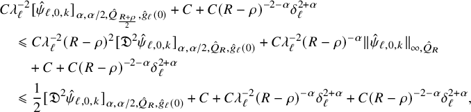 $$ \begin{align}\begin{aligned} &C\lambda_{\ell}^{-2}[\hat{\psi}_{\ell,0,k}]_{{\alpha},{\alpha}/2,\hat{Q}_{\frac{R+\rho}{2}},\hat{g}_{\ell}(0)}+C+C(R-\rho)^{-2-{\alpha}}\delta_{\ell}^{2+\alpha}\\&\quad \leqslant C\lambda_{\ell}^{-2}(R-\rho)^{2}[\mathfrak{D}^2\hat{\psi}_{\ell,0,k}]_{{\alpha},{\alpha}/2,\hat{Q}_R,\hat{g}_{\ell}(0)}+C\lambda_{\ell}^{-2}(R-\rho)^{-{\alpha}}\|\hat{\psi}_{\ell,0,k}\|_{\infty, \hat{Q}_R}\\&\qquad +C+C(R-\rho)^{-2-{\alpha}}\delta_{\ell}^{2+\alpha}\\&\quad \leqslant\frac{1}{2}[\mathfrak{D}^2\hat{\psi}_{\ell,0,k}]_{{\alpha},{\alpha}/2,\hat{Q}_R,\hat{g}_{\ell}(0)}+C+C\lambda_{\ell}^{-2}(R-\rho)^{-{\alpha}}\delta_{\ell}^{2+\alpha}+C(R-\rho)^{-2-{\alpha}}\delta_{\ell}^{2+\alpha}, \end{aligned} \end{align} $$
and after combining (4.140) and (4.141), we can apply the iteration lemma in [Reference Hein and Tosatti21, Lemma 2.9] and deduce that for every
 $\rho <R$
, we have
$\rho <R$
, we have
 $$ \begin{align} [\mathfrak{D}^2\hat{\psi}_{\ell,0,k}]_{{\alpha},{\alpha}/2,\hat{Q}_\rho,\hat{g}_{\ell}(0)}\leqslant C+C\lambda_{\ell}^{-2}(R-\rho)^{-{\alpha}}\delta_{\ell}^{2+\alpha}+C(R-\rho)^{-2-{\alpha}}\delta_{\ell}^{2+\alpha}, \end{align} $$
so in particular, for any fixed R, we deduce that
 $$ \begin{align} [\mathfrak{D}^2\hat{\psi}_{\ell,0,k}]_{{\alpha},{\alpha}/2,\hat{Q}_R,\hat{g}_{\ell}(0)}\leqslant C, \end{align} $$
and finally applying Proposition 2.6 and translating to the tilde picture, we get
 $$ \begin{align} d_{\ell}^{-{\alpha}}\| \mathfrak{D}^{\iota}\tilde \psi_{\ell,j,k} \|_{\infty,\tilde Q_{Rd_{\ell}^{-1}},\tilde g_{\ell}(0)}\leqslant C \varepsilon_{\ell}^{2+{\alpha}-\iota},\quad d_{\ell}^{-{\alpha}}[ \mathfrak{D}^{\iota}\tilde \psi_{\ell,j,k} ]_{{\alpha},{\alpha}/2,\tilde Q_{Rd_{\ell}^{-1}},\tilde g_{\ell}(0)}\leqslant C \varepsilon_{\ell}^{2-\iota} \end{align} $$
for any
 $0\leqslant \iota \leqslant 2$
.
$0\leqslant \iota \leqslant 2$
.
Next, when
 $j\geqslant 1$
, from the Hölder seminorm bound for
$j\geqslant 1$
, from the Hölder seminorm bound for
 $\mathfrak {D}^{2j+2}\hat {\psi }_{\ell , j,k}$
in (4.61), together with Proposition 2.6, we obtain bounds for the lower-order derivatives of
$\mathfrak {D}^{2j+2}\hat {\psi }_{\ell , j,k}$
in (4.61), together with Proposition 2.6, we obtain bounds for the lower-order derivatives of
 $\hat {\psi }_{\ell ,j,k}$
, which in the tilde picture translate to
$\hat {\psi }_{\ell ,j,k}$
, which in the tilde picture translate to
 $$ \begin{align} d_{\ell}^{-2j-{\alpha}}\| \mathfrak{D}^{\iota}\tilde \psi_{\ell,j,k} \|_{\infty,\tilde Q_{Rd_{\ell}^{-1}},\tilde g_{\ell}(0)}\leqslant C \varepsilon_{\ell}^{2j+2+{\alpha}-\iota},\quad d_{\ell}^{-2j-{\alpha}}[ \mathfrak{D}^{\iota}\tilde \psi_{\ell,j,k} ]_{{\alpha},{\alpha}/2,\tilde Q_{Rd_{\ell}^{-1}},\tilde g_{\ell}(0)}\leqslant C \varepsilon_{\ell}^{2j+2-\iota}, \end{align} $$
for any
 $0\leqslant \iota \leqslant 2j+2$
. Observe that these are formally the same as (4.144) when
$0\leqslant \iota \leqslant 2j+2$
. Observe that these are formally the same as (4.144) when
 $j=0$
.
$j=0$
.
4.10.2 Estimates for
$\underline{\tilde {\chi }_{\ell }}$

By Lemma 4.1 (ii),(iii),
 $$ \begin{align} \left\{\begin{array}{ll}\|{i\partial\bar\partial} \underline{\tilde{\chi}_{\ell}} \|_{\infty, \tilde Q_{Rd_{\ell}^{-1}},\tilde g_{\ell}(0)}= \|e^{d_{\ell}^2\lambda_{\ell}^{-2}\tilde t}{i\partial\bar\partial} \underline{\tilde{\varphi}_{\ell}} \|_{\infty, \tilde Q_{Rd_{\ell}^{-1}},\tilde g_{\ell}(0)}= o(1),\\[2mm]\|\partial_{\tilde t}\underline{\tilde{\chi}_{\ell}} \|_{\infty, \tilde Q_{Rd_{\ell}^{-1}},\tilde g_{\ell}(0)}= \|e^{d_{\ell}^2\lambda_{\ell}^{-2}\tilde t} (\partial_{\tilde t} \underline{\tilde{\varphi}_{\ell}}+d_{\ell}^2\lambda_{\ell}^{-2} \underline{\tilde{\varphi}_{\ell}}) \|_{\infty, \tilde Q_{Rd_{\ell}^{-1}},\tilde g_{\ell}(0)}= o(1).\end{array}\right. \end{align} $$
When
 $j=0$
, we have
$j=0$
, we have
 $$ \begin{align} \begin{aligned}d_{\ell}^{-{\alpha}}[\partial_{\tilde t}\underline{\tilde{\chi}_{\ell}}]_{{\alpha},{\alpha}/2,\tilde Q_{Rd_{\ell}^{-1}},\tilde g_{\ell}(0)}&=d_{\ell}^{-{\alpha}}\left[e^{d_{\ell}^2\lambda_{\ell}^{-2}\tilde t} (\partial_{\tilde t} \underline{\tilde{\varphi}_{\ell}}+d_{\ell}^2\lambda_{\ell}^{-2} \underline{\tilde{\varphi}_{\ell}})\right]_{{\alpha},{\alpha}/2,\tilde Q_{Rd_{\ell}^{-1}},\tilde g_{\ell}(0)}\\&\leqslant d_{\ell}^{-{\alpha}}\left[e^{d_{\ell}^2\lambda_{\ell}^{-2}\tilde t} \right]_{{\alpha},{\alpha}/2,\tilde Q_{Rd_{\ell}^{-1}},\tilde g_{\ell}(0)}\|\partial_{\tilde t} \underline{\tilde{\varphi}_{\ell}}+d_{\ell}^2\lambda_{\ell}^{-2} \underline{\tilde{\varphi}_{\ell}}\|_{\infty, \tilde Q_{Rd_{\ell}^{-1}},\tilde g_{\ell}(0)}\\&\quad +d_{\ell}^{-{\alpha}}\left\|e^{d_{\ell}^2\lambda_{\ell}^{-2}\tilde t} \right\|_{\infty,\tilde Q_{Rd_{\ell}^{-1}},\tilde g_{\ell}(0)}[\partial_{\tilde t} \underline{\tilde{\varphi}_{\ell}}+d_{\ell}^2\lambda_{\ell}^{-2} \underline{\tilde{\varphi}_{\ell}}]_{{\alpha},{\alpha}/2, \tilde Q_{Rd_{\ell}^{-1}},\tilde g_{\ell}(0)}\\&\leqslant o(1) Cd_{\ell}^{-{\alpha}}(d_{\ell} \lambda_{\ell}^{-1})^{\alpha}+o(1)=o(1),\end{aligned} \end{align} $$
where we used
 $d_{\ell }^{-{\alpha }}[\partial _{\tilde t} \underline{\tilde {\varphi }_{\ell }}+d_{\ell }^2\lambda _{\ell }^{-2} \underline{\tilde {\varphi }_{\ell }}]_{{\alpha },{\alpha }/2, \tilde Q_{Rd_{\ell }^{-1}},\tilde g_{\ell }(0)}=o(1)$
, which follows from (4.137). Similarly,
$d_{\ell }^{-{\alpha }}[\partial _{\tilde t} \underline{\tilde {\varphi }_{\ell }}+d_{\ell }^2\lambda _{\ell }^{-2} \underline{\tilde {\varphi }_{\ell }}]_{{\alpha },{\alpha }/2, \tilde Q_{Rd_{\ell }^{-1}},\tilde g_{\ell }(0)}=o(1)$
, which follows from (4.137). Similarly,
 $$ \begin{align}\begin{aligned} d_{\ell}^{-{\alpha}}[{i\partial\bar\partial}\underline{\tilde{\chi}_{\ell}}]_{{\alpha},{\alpha}/2,\tilde Q_{Rd_{\ell}^{-1}},\tilde g_{\ell}(0)}&=d_{\ell}^{-{\alpha}}\left[e^{d_{\ell}^2\lambda_{\ell}^{-2}\tilde t} {i\partial\bar\partial} \underline{\tilde{\varphi}_{\ell}}\right]_{{\alpha},{\alpha}/2,\tilde Q_{Rd_{\ell}^{-1}},\tilde g_{\ell}(0)}\\&\leqslant d_{\ell}^{-{\alpha}}\left[e^{d_{\ell}^2\lambda_{\ell}^{-2}\tilde t} \right]_{{\alpha},{\alpha}/2,\tilde Q_{Rd_{\ell}^{-1}},\tilde g_{\ell}(0)}\|{i\partial\bar\partial} \underline{\tilde{\varphi}_{\ell}}\|_{\infty, \tilde Q_{Rd_{\ell}^{-1}},\tilde g_{\ell}(0)}\\&\quad +d_{\ell}^{-{\alpha}}\left\|e^{d_{\ell}^2\lambda_{\ell}^{-2}\tilde t} \right\|_{\infty,\tilde Q_{Rd_{\ell}^{-1}},\tilde g_{\ell}(0)}[{i\partial\bar\partial} \underline{\tilde{\varphi}_{\ell}}]_{{\alpha},{\alpha}/2, \tilde Q_{Rd_{\ell}^{-1}},\tilde g_{\ell}(0)}\\&\leqslant o(1) Cd_{\ell}^{-{\alpha}}(d_{\ell} \lambda_{\ell}^{-1})^{\alpha}+C\leqslant C, \end{aligned}\end{align} $$
where we used
 $d_{\ell }^{-{\alpha }}[{i\partial \bar \partial }\underline{\tilde {\varphi }_{\ell }}]_{{\alpha },{\alpha }/2, \tilde Q_{Rd_{\ell }^{-1}},\tilde g_{\ell }(0)}\leqslant C$
, which follows from (4.108). Thus, when
$d_{\ell }^{-{\alpha }}[{i\partial \bar \partial }\underline{\tilde {\varphi }_{\ell }}]_{{\alpha },{\alpha }/2, \tilde Q_{Rd_{\ell }^{-1}},\tilde g_{\ell }(0)}\leqslant C$
, which follows from (4.108). Thus, when
 $j=0$
, we have
$j=0$
, we have
 $$ \begin{align} [{i\partial\bar\partial} \underline{\tilde{\chi}_{\ell}}]_{{\alpha},{\alpha}/2,\tilde Q_{Rd_{\ell}^{-1}},\tilde g_{\ell}(0)}\leqslant Cd_{\ell}^{{\alpha}},\quad [\partial_{\tilde t} \underline{\tilde{\chi}_{\ell}}]_{{\alpha},{\alpha}/2,\tilde Q_{Rd_{\ell}^{-1}},\tilde g_{\ell}(0)}=o(d_{\ell}^{{\alpha}}). \end{align} $$
When
 $j\geqslant 1$
, from (4.109), (4.116) and (4.117), we obtain the analogous seminorm bounds
$j\geqslant 1$
, from (4.109), (4.116) and (4.117), we obtain the analogous seminorm bounds
 $$ \begin{align} [\mathfrak{D}^{2j} {i\partial\bar\partial} \underline{\tilde{\chi}_{\ell}}]_{{\alpha},{\alpha}/2,\tilde Q_{Rd_{\ell}^{-1}},\tilde g_{\ell}(0)}\leqslant Cd_{\ell}^{2j+{\alpha}},\quad [\mathfrak{D}^{2j} \partial_{\tilde t} \underline{\tilde{\chi}_{\ell}}]_{{\alpha},{\alpha}/2,\tilde Q_{Rd_{\ell}^{-1}},\tilde g_{\ell}(0)}\leqslant Cd_{\ell}^{2j+{\alpha}}, \end{align} $$
and we can interpolate between these and (4.146) to conclude that
 $$ \begin{align} \left\{ \begin{array}{ll} d_{\ell}^{-\iota} \|\mathfrak{D}^\iota {i\partial\bar\partial} \underline{\tilde{\chi}_{\ell}}\|_{\infty, \tilde Q_{Rd_{\ell}^{-1}},\tilde g_{\ell}(0)}=o(1),\quad 0\leqslant \iota\leqslant 2j,\\[2mm] d_{\ell}^{-\iota} \|\mathfrak{D}^\iota \partial_{\tilde t} \underline{\tilde{\chi}_{\ell}}\|_{\infty, \tilde Q_{Rd_{\ell}^{-1}},\tilde g_{\ell}(0)}=o(1),\quad 0\leqslant \iota\leqslant 2j,\\[2mm] d_{\ell}^{-\iota-{\alpha}} [\mathfrak{D}^\iota {i\partial\bar\partial} \underline{\tilde{\chi}_{\ell}}]_{{\alpha},{\alpha}/2, \tilde Q_{Rd_{\ell}^{-1}},\tilde g_{\ell}(0)}=o(1),\quad 0\leqslant \iota<2j, \\[2mm] d_{\ell}^{-\iota-{\alpha}} [\mathfrak{D}^\iota \partial_{\tilde t} \underline{\tilde{\chi}_{\ell}}]_{{\alpha},{\alpha}/2, \tilde Q_{Rd_{\ell}^{-1}},\tilde g_{\ell}(0)}=o(1),\quad 0\leqslant \iota<2j \end{array} \right. \end{align} $$
We now treat
 $\tilde {\chi }_{\ell }^{*}$
. From (4.149), (4.150) and the definition of
$\tilde {\chi }_{\ell }^{*}$
. From (4.149), (4.150) and the definition of
 $\tilde {\chi }_{\ell }^{*}$
we see that for all
$\tilde {\chi }_{\ell }^{*}$
we see that for all
 $j\geqslant 0$
,
$j\geqslant 0$
,
 $$ \begin{align} [\mathfrak{D}^{2j} {i\partial\bar\partial} \underline{\tilde{\chi}_{\ell}^{*}}]_{{\alpha},{\alpha}/2,\tilde Q_{Rd_{\ell}^{-1}},\tilde g_{\ell}(0)}\leqslant Cd_{\ell}^{2j+{\alpha}},\quad [\mathfrak{D}^{2j} \partial_{\tilde t} \underline{\tilde{\chi}_{\ell}^{*}}]_{{\alpha},{\alpha}/2,\tilde Q_{Rd_{\ell}^{-1}},\tilde g_{\ell}(0)}\leqslant Cd_{\ell}^{2j+{\alpha}}. \end{align} $$
Using these and Lemma 2.4, we get
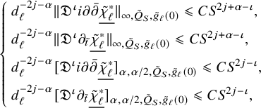 $$ \begin{align} \left\{ \begin{array}{ll} d_{\ell}^{-2j-{\alpha}} \|\mathfrak{D}^\iota {i\partial\bar\partial} \underline{\tilde{\chi}_{\ell}^{*}}\|_{\infty, \tilde Q_{S},\tilde g_{\ell}(0)}\leqslant CS^{2j+{\alpha}-\iota},\\[2mm] d_{\ell}^{-2j-{\alpha}} \|\mathfrak{D}^\iota \partial_{\tilde t} \underline{\tilde{\chi}_{\ell}^{*}}\|_{\infty, \tilde Q_{S},\tilde g_{\ell}(0)}\leqslant CS^{2j+{\alpha}-\iota} ,\\[2mm] d_{\ell}^{-2j-{\alpha}} [\mathfrak{D}^\iota {i\partial\bar\partial} \underline{\tilde{\chi}_{\ell}^{*}}]_{{\alpha},{\alpha}/2, \tilde Q_{S},\tilde g_{\ell}(0)} \leqslant CS^{2j-\iota},\\ [2mm] d_{\ell}^{-2j-{\alpha}} [\mathfrak{D}^\iota \partial_{\tilde t} \underline{\tilde{\chi}_{\ell}^{*}}]_{{\alpha},{\alpha}/2, \tilde Q_{S},\tilde g_{\ell}(0)} \leqslant CS^{2j-\iota}, \end{array} \right. \end{align} $$
for all
 $0\leqslant \iota \leqslant 2j$
and
$0\leqslant \iota \leqslant 2j$
and
 $0<S\leqslant Rd_{\ell }^{-1}$
.
$0<S\leqslant Rd_{\ell }^{-1}$
.
We will also need a bound for the
 $L^\infty $
norm of derivatives of
$L^\infty $
norm of derivatives of
 $d_{\ell }^{-2j-{\alpha }}\underline{\tilde {\chi }_{\ell }^{*}}$
of order up to
$d_{\ell }^{-2j-{\alpha }}\underline{\tilde {\chi }_{\ell }^{*}}$
of order up to
 $2j+2$
, which in general may blow up, but which will nevertheless be useful later. To start, from Lemma 4.1 (ii), we have
$2j+2$
, which in general may blow up, but which will nevertheless be useful later. To start, from Lemma 4.1 (ii), we have
 $\|\underline{\hat {\chi }_{\ell }}\|_{\infty , \hat {Q}_R}=o(1)\lambda _{\ell }^2,$
while from (4.152), we see in particular that
$\|\underline{\hat {\chi }_{\ell }}\|_{\infty , \hat {Q}_R}=o(1)\lambda _{\ell }^2,$
while from (4.152), we see in particular that
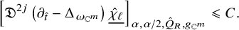 $$ \begin{align} \left[\mathfrak{D}^{2j}\left(\partial_{\hat{t}}-\Delta_{\omega_{\mathbb{C}^m}}\right)\underline{\hat{\chi}_{\ell}}\right]_{{\alpha},{\alpha}/2,\hat{Q}_R,g_{\mathbb{C}^m}}\leqslant C. \end{align} $$
Standard Euclidean Schauder estimates then imply that
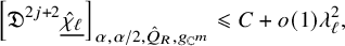 $$ \begin{align} \left[\mathfrak{D}^{2j+2}\underline{\hat{\chi}_{\ell}}\right]_{{\alpha},{\alpha}/2,\hat{Q}_R,g_{\mathbb{C}^m}}\leqslant C+o(1)\lambda_{\ell}^2, \end{align} $$
and since we may assume without loss that
 $o(1)\lambda _{\ell }^2\geqslant C$
, passing to the tilde picture, we get
$o(1)\lambda _{\ell }^2\geqslant C$
, passing to the tilde picture, we get
 $$ \begin{align} d_{\ell}^{-2j-{\alpha}}\left[\mathfrak{D}^{2j+2}\underline{\tilde{\chi}^{*}_{\ell}}\right]_{{\alpha},{\alpha}/2,\tilde{Q}_{Rd_{\ell}^{-1}},g_{\mathbb{C}^m}} =d_{\ell}^{-2j-{\alpha}}\left[\mathfrak{D}^{2j+2}\underline{\tilde{\chi}_{\ell}}\right]_{{\alpha},{\alpha}/2,\tilde{Q}_{Rd_{\ell}^{-1}},g_{\mathbb{C}^m}}\leqslant o(1)\lambda_{\ell}^2, \end{align} $$
and we can then apply Lemma 2.4 to
 $\tilde {Q}_R$
and get
$\tilde {Q}_R$
and get
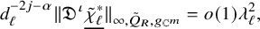 $$ \begin{align} d_{\ell}^{-2j-{\alpha}}\|\mathfrak{D}^\iota\underline{\tilde{\chi}^{*}_{\ell}}\|_{\infty,\tilde{Q}_R,g_{\mathbb{C}^m}}= o(1)\lambda_{\ell}^2, \end{align} $$
for
 $0\leqslant \iota \leqslant 2j+2$
.
$0\leqslant \iota \leqslant 2j+2$
.
Since
 $\underline{\tilde {\chi }^\sharp _{\ell }}$
is a jet of
$\underline{\tilde {\chi }^\sharp _{\ell }}$
is a jet of
 $\underline{\tilde {\chi }_{\ell }}$
, it inherits from (4.146) and (4.151) the bounds
$\underline{\tilde {\chi }_{\ell }}$
, it inherits from (4.146) and (4.151) the bounds
 $$ \begin{align} \left\{ \begin{array}{ll} d_{\ell}^{-\iota} \|\mathfrak{D}^\iota {i\partial\bar\partial} \underline{\tilde{\chi}_{\ell}^\sharp}\|_{\infty, \tilde Q_{Rd_{\ell}^{-1}},\tilde g_{\ell}(0)}=o(1) ,\\ [2mm] d_{\ell}^{-\iota} \|\mathfrak{D}^\iota \partial_{\tilde t} \underline{\tilde{\chi}_{\ell}^\sharp}\|_{\infty, \tilde Q_{Rd_{\ell}^{-1}},\tilde g_{\ell}(0)}=o(1) ,\\[2mm] d_{\ell}^{-\iota-{\alpha}} [\mathfrak{D}^\iota {i\partial\bar\partial} \underline{\tilde{\chi}_{\ell}^\sharp}]_{{\alpha},{\alpha}/2, \tilde Q_{Rd_{\ell}^{-1}},\tilde g_{\ell}(0)} =o(1) ,\\[2mm] d_{\ell}^{-\iota-{\alpha}} [\mathfrak{D}^\iota \partial_{\tilde t} \underline{\tilde{\chi}_{\ell}^\sharp}]_{{\alpha},{\alpha}/2, \tilde Q_{Rd_{\ell}^{-1}},\tilde g_{\ell}(0)} =o(1), \end{array} \right. \end{align} $$
for all
 $0\leqslant \iota \leqslant 2j$
and R fixed. Moreover, since
$0\leqslant \iota \leqslant 2j$
and R fixed. Moreover, since
 $\underline{\tilde {\chi }_{\ell }^\sharp }$
is a polynomial of degree at most
$\underline{\tilde {\chi }_{\ell }^\sharp }$
is a polynomial of degree at most
 $2j+2$
, it vanishes when differentiated more than
$2j+2$
, it vanishes when differentiated more than
 $2j+2$
times.
$2j+2$
times.
Furthermore, recalling the definitions of
 $\tilde {\eta }^\ddagger _{\ell }$
and
$\tilde {\eta }^\ddagger _{\ell }$
and
 $\tilde {\eta }^\diamondsuit _{\ell }$
in (4.125), from (4.153) and (4.158), we quickly deduce
$\tilde {\eta }^\diamondsuit _{\ell }$
in (4.125), from (4.153) and (4.158), we quickly deduce
 $$ \begin{align} d_{\ell}^{-2j-{\alpha}}\|\mathfrak{D}^\iota\tilde{\eta}^\diamondsuit_{\ell}\|_{\infty, \tilde Q_{S},\tilde g_{\ell}(0)}\leqslant CS^{2j+{\alpha}-\iota},\quad d_{\ell}^{-2j-{\alpha}}[\mathfrak{D}^\iota\tilde{\eta}^\diamondsuit_{\ell}]_{{\alpha},{\alpha}/2, \tilde Q_{S},\tilde g_{\ell}(0)}\leqslant CS^{2j-\iota} \end{align} $$
for
 $0\leqslant \iota \leqslant 2j, 0<S\leqslant Rd_{\ell }^{-1}$
, and
$0\leqslant \iota \leqslant 2j, 0<S\leqslant Rd_{\ell }^{-1}$
, and
 $$ \begin{align} d_{\ell}^{-\iota}\|\mathfrak{D}^\iota\tilde{\eta}^\ddagger_{\ell}\|_{\infty, \tilde Q_{Rd_{\ell}^{-1}},\tilde g_{\ell}(0)}=o(1),\quad d_{\ell}^{-\iota-{\alpha}}[\mathfrak{D}^\iota\tilde{\eta}^\ddagger_{\ell}]_{{\alpha},{\alpha}/2, \tilde Q_{Rd_{\ell}^{-1}},\tilde g_{\ell}(0)}=o(1), \end{align} $$
also for
 $0\leqslant \iota \leqslant 2j$
, R fixed (and derivatives of
$0\leqslant \iota \leqslant 2j$
, R fixed (and derivatives of
 $\tilde {\eta }^\ddagger _{\ell }$
of order higher than
$\tilde {\eta }^\ddagger _{\ell }$
of order higher than
 $2j$
vanish, of course).
$2j$
vanish, of course).
4.10.3 Estimates for
$\tilde A_{\ell ,i,p,k}^{*}$

From (4.131), we have
 $$ \begin{align} [\mathfrak{D}^{2j} \hat A^{*}_{\ell,i,p,k}]_{{\alpha},{\alpha}/2,\hat Q_{R},\hat g_{\ell}( 0)} \leqslant C \delta_{\ell}^2, \end{align} $$
and hence, Lemma 2.4 implies
 $$ \begin{align} \|\mathfrak{D}^{\iota} \hat A^{*}_{\ell,i,p,k}\|_{\infty,\hat Q_{R},\hat g_{\ell}( 0)} \leqslant C\delta_{\ell}^2 R^{2j+{\alpha}-\iota},\quad [\mathfrak{D}^{\iota} \hat A^{*}_{\ell,i,p,k}]_{{\alpha},{\alpha}/2,\hat Q_{R},\hat g_{\ell}( 0)} \leqslant C\delta_{\ell}^2 R^{2j-\iota} \end{align} $$
for all
 $0\leqslant \iota \leqslant 2j$
and fixed
$0\leqslant \iota \leqslant 2j$
and fixed
 $R>0$
. Taking
$R>0$
. Taking
 $R=S d_{\ell }$
and transferring to the tilde picture, we have
$R=S d_{\ell }$
and transferring to the tilde picture, we have
 $$ \begin{align} d_{\ell}^{-\iota} \|\mathfrak{D}^{\iota} \tilde A^{*}_{\ell,i,p,k}\|_{\infty,\tilde Q_{S},\tilde g_{\ell}( 0)} \leqslant C\varepsilon_{\ell}^2 (d_{\ell} S)^{2j+{\alpha}-\iota},\quad d_{\ell}^{-\iota-{\alpha}}[\mathfrak{D}^{\iota} \tilde A^{*}_{\ell,i,p,k}]_{{\alpha},{\alpha}/2,\tilde Q_{S},\tilde g_{\ell}( 0)} \leqslant C\varepsilon_{\ell}^2 (d_{\ell} S)^{2j-\iota} \end{align} $$
for all
 $0\leqslant \iota \leqslant 2j$
and
$0\leqslant \iota \leqslant 2j$
and
 $S\leqslant R d_{\ell }^{-1}$
.
$S\leqslant R d_{\ell }^{-1}$
.
For higher order derivatives of
 $\tilde A_{\ell ,i,p,k}^{*}$
, we use interpolation. Since
$\tilde A_{\ell ,i,p,k}^{*}$
, we use interpolation. Since
 $\tilde A^\sharp _{\ell ,i,p,k}$
is a parabolic polynomial of degree at most
$\tilde A^\sharp _{\ell ,i,p,k}$
is a parabolic polynomial of degree at most
 $2j$
, (4.131) implies
$2j$
, (4.131) implies
 $$ \begin{align} \left[\mathfrak{D}^{2j+\iota} \hat A^{*}_{\ell,i,p,k}\right]_{{\alpha},{\alpha}/2,\hat Q_{R},\hat g_{\ell}( 0)} \leqslant C \delta_{\ell}^{2-\iota} \end{align} $$
for all
 $0\leqslant \iota \leqslant 2k+2$
. For any
$0\leqslant \iota \leqslant 2k+2$
. For any
 $1\leqslant \iota \leqslant 2k+2$
, Proposition 2.3 in the hat picture gives for
$1\leqslant \iota \leqslant 2k+2$
, Proposition 2.3 in the hat picture gives for
 $0<\rho _1<\rho _2\leqslant R$
,
$0<\rho _1<\rho _2\leqslant R$
,
 $$ \begin{align} \begin{aligned} &(\rho_2-\rho_1)^\iota \|\mathfrak{D}^{2j+\iota} \hat A^{*}_{\ell,i,p,k}\|_{\infty,\hat Q_{\rho_1},\hat g_{\ell}( 0)}\\&\quad\leqslant C\left((\rho_2-\rho_1)^{\iota+{\alpha}} [\mathfrak{D}^{2j+\iota} \hat A^{*}_{\ell,i,p,k}]_{{\alpha},{\alpha}/2,\hat Q_{\rho_2},\hat g_{\ell}( 0)}+\|\mathfrak{D}^{2j} \hat A^{*}_{\ell,i,p,k}\|_{\infty,\hat Q_{\rho_2},\hat g_{\ell}( 0)} \right)\\&\quad\leqslant C(\rho_2-\rho_1)^{\iota+{\alpha}} \delta_{\ell}^{2-\iota}+C\delta_{\ell}^2 \rho_2^{{\alpha}}. \end{aligned} \end{align} $$
We can follow closely the choice of
 $\rho _i$
in the interpolation in [Reference Hein and Tosatti21, §4.9.3] (with j replaced by
$\rho _i$
in the interpolation in [Reference Hein and Tosatti21, §4.9.3] (with j replaced by
 $2j$
here) to conclude that
$2j$
here) to conclude that
 $$ \begin{align} \|\mathfrak{D}^{2j+\iota} \hat A^{*}_{\ell,i,p,k}\|_{\infty,\hat Q_{S\delta_{\ell}},\hat g_{\ell}(0)}\leqslant C_S \delta_{\ell}^{2+{\alpha}-\iota}. \end{align} $$
This will play an important role in case
 $\varepsilon _{\ell }\geqslant C^{-1}$
. For later purposes, we will need to estimate the dependence of
$\varepsilon _{\ell }\geqslant C^{-1}$
. For later purposes, we will need to estimate the dependence of
 $C_S$
on S as
$C_S$
on S as
 $S\to +\infty $
. In fact,
$S\to +\infty $
. In fact,
 $C_S$
in [Reference Hein and Tosatti21, (4.127)] is given by
$C_S$
in [Reference Hein and Tosatti21, (4.127)] is given by
 $C(AS)^{\frac {{\alpha }^2}{\iota +{\alpha }}}$
where
$C(AS)^{\frac {{\alpha }^2}{\iota +{\alpha }}}$
where
 $A>1$
is given as a function of
$A>1$
is given as a function of
 $S>1$
by solving the equation
$S>1$
by solving the equation
 $(A-1)^{-1}A^{\frac {{\alpha }}{\iota +{\alpha }}}= S^{\frac {\iota }{\iota +{\alpha }}}$
. Since
$(A-1)^{-1}A^{\frac {{\alpha }}{\iota +{\alpha }}}= S^{\frac {\iota }{\iota +{\alpha }}}$
. Since
 $\frac {{\alpha }}{\iota +{\alpha }}<1$
for
$\frac {{\alpha }}{\iota +{\alpha }}<1$
for
 $\iota \geqslant 1$
, A stays bounded as
$\iota \geqslant 1$
, A stays bounded as
 $S\to +\infty $
. Hence, we can estimate
$S\to +\infty $
. Hence, we can estimate
 $C_S$
from above by
$C_S$
from above by
 $$ \begin{align} C_S\leqslant C(AS)^{\frac{{\alpha}^2}{\iota+{\alpha}}}\leqslant CS^{\alpha} \end{align} $$
for
 $S>1$
. Therefore, in the tilde picture we obtain
$S>1$
. Therefore, in the tilde picture we obtain
 $$ \begin{align} \|\mathfrak{D}^{2j+\iota} \tilde A^{*}_{\ell,i,p,k}\|_{\infty,\tilde Q_{S\varepsilon_{\ell}},\tilde g_{\ell}(0)}\leqslant CS^{\alpha}\varepsilon_{\ell}^{2-\iota+{\alpha}} d_{\ell}^{2j+{\alpha}}, \end{align} $$
where
 $1\leqslant \iota \leqslant 2k+2$
and
$1\leqslant \iota \leqslant 2k+2$
and
 $S>1$
fixed (which is the analog of [Reference Hein and Tosatti21, (4.129)]).
$S>1$
fixed (which is the analog of [Reference Hein and Tosatti21, (4.129)]).
Similarly, in the case when
 $\varepsilon _{\ell }\to 0$
, following the derivation of [Reference Hein and Tosatti21, (4.132)], we obtain
$\varepsilon _{\ell }\to 0$
, following the derivation of [Reference Hein and Tosatti21, (4.132)], we obtain
 $$ \begin{align} \|\mathfrak{D}^{2j+\iota} \hat A^{*}_{\ell,i,p,k}\|_{\infty,\hat Q_{S d_{\ell}},\hat g_{\ell}(0)}\leqslant C\delta_{\ell}^{2-\iota}d_{\ell}^{\alpha} \varepsilon_{\ell}^{\frac{\iota{\alpha}}{\iota+{\alpha}}}S^{\frac{{\alpha}^2}{\iota+{\alpha}}}, \end{align} $$
which in the tilde picture becomes
 $$ \begin{align} \|\mathfrak{D}^{2j+\iota} \tilde A^{*}_{\ell,i,p,k}\|_{\infty,\tilde Q_{S},\tilde g_{\ell}(0)}\leqslant C \varepsilon_{\ell}^{2-\iota} (S^{\alpha} \varepsilon_{\ell}^\iota)^{\frac{{\alpha}}{\iota+{\alpha}}} d_{\ell}^{2j+{\alpha}} \end{align} $$
for
 $1\leqslant \iota \leqslant 2k+2$
and
$1\leqslant \iota \leqslant 2k+2$
and
 $S>1$
fixed.
$S>1$
fixed.
4.10.4 Estimates for
$\tilde A_{\ell ,i,p,k}^\sharp $

By (4.73), we have for all
 $0\leqslant \iota \leqslant 2j$
that
$0\leqslant \iota \leqslant 2j$
that
 $$ \begin{align} \|\mathfrak{D}^\iota\hat A_{\ell,i,p,k}\|_{\infty,\hat Q_{R},\hat g_{\ell}(0)}\leqslant C\delta_{\ell}^2\left( e^{\frac{-2i+2-{\alpha}}{2}t_{\ell}}\right)^{1-\frac{\iota}{2j+{\alpha}}} \end{align} $$
for all given
 $R>0$
(with C independent of
$R>0$
(with C independent of
 $R>0$
). Since
$R>0$
). Since
 $\hat A_{\ell ,i,p,k}^\sharp $
is the
$\hat A_{\ell ,i,p,k}^\sharp $
is the
 $2j$
-jet of
$2j$
-jet of
 $\hat A_{\ell ,i,p,k}$
at
$\hat A_{\ell ,i,p,k}$
at
 $(0,0)$
, we see that all the coefficients of the polynomial
$(0,0)$
, we see that all the coefficients of the polynomial
 $\hat A_{\ell ,i,p,k}^\sharp $
are bounded by
$\hat A_{\ell ,i,p,k}^\sharp $
are bounded by
 $C\delta _{\ell }^2 e^{\frac {-2i+2-{\alpha }}{2}\cdot \frac {{\alpha } }{2j+{\alpha }}t_{\ell }}$
, and so
$C\delta _{\ell }^2 e^{\frac {-2i+2-{\alpha }}{2}\cdot \frac {{\alpha } }{2j+{\alpha }}t_{\ell }}$
, and so
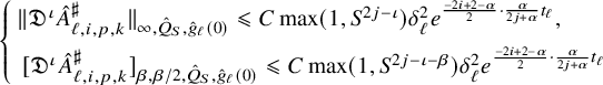 $$ \begin{align} \left\{ \begin{array}{ll} \|\mathfrak{D}^\iota \hat A_{\ell,i,p,k}^\sharp\|_{\infty,\hat Q_{S},\hat g_{\ell}(0)}\leqslant C \max( 1, S^{2j-\iota}) \delta_{\ell}^2 e^{\frac{-2i+2-{\alpha}}{2}\cdot \frac{{\alpha} }{2j+{\alpha}}t_{\ell}},\\[2mm] \, [\mathfrak{D}^\iota \hat A_{\ell,i,p,k}^\sharp]_{{\beta},{\beta}/2,\hat Q_{S},\hat g_{\ell}(0)}\leqslant C \max( 1, S^{2j-\iota-{\beta}})\delta_{\ell}^2 e^{\frac{-2i+2-{\alpha}}{2}\cdot \frac{{\alpha} }{2j+{\alpha}}t_{\ell}} \end{array} \right. \end{align} $$
for all
 $S>0$
,
$S>0$
,
 $0\leqslant \iota \leqslant 2j$
and
$0\leqslant \iota \leqslant 2j$
and
 $0<{\beta }<1$
. Transferring to the tilde picture yields
$0<{\beta }<1$
. Transferring to the tilde picture yields
 $$ \begin{align} \left\{ \begin{array}{ll} d_{\ell}^{-\iota+2}\|\mathfrak{D}^\iota \tilde A_{\ell,i,p,k}^\sharp\|_{\infty,\tilde Q_{S},\tilde g_{\ell}(0)}\leqslant C \max( 1, (Sd_{\ell})^{2j-\iota}) \delta_{\ell}^2 e^{\frac{-2i+2-{\alpha}}{2}\cdot \frac{{\alpha} }{2j+{\alpha}}t_{\ell}},\\ [2mm] \, d_{\ell}^{-\iota+2-{\beta}}[\mathfrak{D}^\iota \tilde A_{\ell,i,p,k}^\sharp]_{{\beta},{\beta}/2,\tilde Q_{S},\tilde g_{\ell}(0)}\leqslant C \max( 1, (Sd_{\ell})^{2j-\iota-{\beta}})\delta_{\ell}^2 e^{\frac{-2i+2-{\alpha}}{2}\cdot \frac{{\alpha} }{2j+{\alpha}}t_{\ell}}, \end{array} \right. \end{align} $$
for all
 $0<S\leqslant Rd_{\ell }^{-1}$
,
$0<S\leqslant Rd_{\ell }^{-1}$
,
 $0\leqslant \iota \leqslant 2j$
and
$0\leqslant \iota \leqslant 2j$
and
 $0<{\beta }<1$
, c.f. [Reference Hein and Tosatti21, (4.135)–(4.136)].
$0<{\beta }<1$
, c.f. [Reference Hein and Tosatti21, (4.135)–(4.136)].
4.10.5 Estimates for
$\tilde {\eta }_{\ell }^\circ $
and its potential

First, we recall that
 $$ \begin{align} \hat \eta_{\ell}^\circ =\sum_{i=1}^j\sum_{p=1}^{N_{i,k}}{i\partial\bar\partial} \hat{\mathfrak{G}}_{\hat{t},k}(\hat A_{\ell,i,p,k}^{*},\hat G_{\ell,i,p,k}). \end{align} $$
Here,
 $\hat {\mathfrak {G}}_{\hat {t},k}$
and
$\hat {\mathfrak {G}}_{\hat {t},k}$
and
 $\hat A_{\ell ,i,p,k}$
are
$\hat A_{\ell ,i,p,k}$
are
 $\hat t$
-dependent while
$\hat t$
-dependent while
 $\hat G_{\ell ,i,p,k}$
is independent of time.
$\hat G_{\ell ,i,p,k}$
is independent of time.
By applying (3.1) for each fixed
 $\hat t$
, we can write
$\hat t$
, we can write
 $$ \begin{align} \hat{\mathfrak{G}}_{\hat{t},k}(\hat A_{\ell,i,p,k}^{*},\hat G_{\ell,i,p,k})= \sum_{\iota=0}^{2k}\sum_{q=\lceil\frac{\iota}{2}\rceil}^{k} e^{-q\lambda_{\ell}^{-2}\hat t-(q-\frac{\iota}{2})t_{\ell}} \delta_{\ell}^\iota \hat \Phi_{\iota,q}(\hat G_{\ell,i,p,k})\circledast {\mathbb{D}}^\iota \hat A_{\ell,i,p,k}^{*}, \end{align} $$
where
 $\hat \Phi _{\iota ,q}(\hat G_{\ell ,i,p,k})$
is independent of time. Note also that
$\hat \Phi _{\iota ,q}(\hat G_{\ell ,i,p,k})$
is independent of time. Note also that
 $\hat J_{\ell }$
is independent of time and hence [Reference Hein and Tosatti21, (4.141), (4.144)] can be directly carried over, so that
$\hat J_{\ell }$
is independent of time and hence [Reference Hein and Tosatti21, (4.141), (4.144)] can be directly carried over, so that
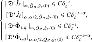 $$ \begin{align} \left\{ \begin{array}{ll} \| \mathfrak{D}^\iota \hat J_{\ell}\|_{\infty, \hat Q_R,\hat g_{\ell}(0)} \leqslant C\delta_{\ell}^{-\iota},\\[2mm] \, [ \mathfrak{D}^\iota \hat J_{\ell}]_{{\alpha},{\alpha}/2, \hat Q_R,\hat g_{\ell}(0)} \leqslant C\delta_{\ell}^{-\iota-{\alpha}},\\[2mm] \| \mathfrak{D}^\iota \hat \Phi_{\iota,q}\|_{\infty, \hat Q_R,\hat g_{\ell}(0)} \leqslant C\delta_{\ell}^{-\iota},\\[2mm] [ \mathfrak{D}^\iota \hat \Phi_{\iota,q}]_{{\alpha},{\alpha}/2, \hat Q_R,\hat g_{\ell}(0)} \leqslant C\delta_{\ell}^{-\iota-{\alpha}}, \end{array} \right. \end{align} $$
for each
 $\iota \geqslant 0,\lceil \frac {\iota }{2}\rceil \leqslant q\leqslant 2k$
and fixed
$\iota \geqslant 0,\lceil \frac {\iota }{2}\rceil \leqslant q\leqslant 2k$
and fixed
 $R>0$
.
$R>0$
.
Schematically, we have
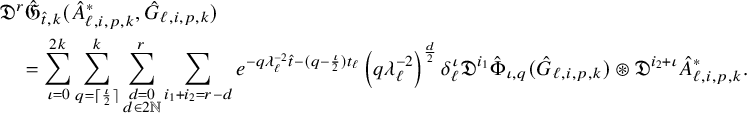 $$ \begin{align} \begin{aligned} &\mathfrak{D}^{r}\hat{\mathfrak{G}}_{\hat{t},k}(\hat A_{\ell,i,p,k}^{*},\hat G_{\ell,i,p,k})\\&\quad= \sum_{\iota=0}^{2k}\sum_{q=\lceil\frac{\iota}{2}\rceil}^{k} \sum_{\substack{d=0\\d\in 2\mathbb{N}}}^r \sum_{i_1+i_2=r-d}e^{-q\lambda_{\ell}^{-2}\hat t-(q-\frac{\iota}{2})t_{\ell}} \left(q\lambda_{\ell}^{-2}\right)^{\frac{d}{2}} \delta_{\ell}^\iota\mathfrak{D}^{i_1}\hat \Phi_{\iota,q}(\hat G_{\ell,i,p,k}) \circledast \mathfrak{D}^{i_2+\iota} \hat A_{\ell,i,p,k}^{*}. \end{aligned} \end{align} $$
To estimate this, we will need (4.162), (4.164) and (4.168):
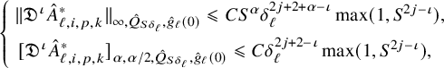 $$ \begin{align} \left\{ \begin{array}{ll} \|\mathfrak{D}^ \iota \hat A^{*}_{\ell,i,p,k}\|_{\infty,\hat Q_{S\delta_{\ell}},\hat g_{\ell}(0)} \leqslant CS^{\alpha}\delta_{\ell}^{2j+2+{\alpha}- \iota }\max( 1, S^{2j-\iota}),\\[2mm] \, [\mathfrak{D}^ \iota \hat A^{*}_{\ell,i,p,k}]_{{\alpha},{\alpha}/2,\hat Q_{ S\delta_{\ell}},\hat g_{\ell}(0)} \leqslant C \delta_{\ell}^{2j+2- \iota } \max(1,S^{2j-\iota}), \end{array} \right. \end{align} $$
for all
 $0\leqslant \iota \leqslant 2k+2+2j$
and
$0\leqslant \iota \leqslant 2k+2+2j$
and
 $S>1$
fixed. Now using (4.176) and (4.178) in (4.177), and recalling that
$S>1$
fixed. Now using (4.176) and (4.178) in (4.177), and recalling that
 $\delta _{\ell }=\lambda _{\ell } e^{-\frac {t_{\ell }}{2}},$
yields
$\delta _{\ell }=\lambda _{\ell } e^{-\frac {t_{\ell }}{2}},$
yields
 $$ \begin{align} \begin{aligned} \|\mathfrak{D}^{r}\hat{\mathfrak{G}}_{\hat{t},k}(\hat A_{\ell,i,p,k}^{*},\hat G_{\ell,i,p,k})\|_{\infty,\hat Q_{S\delta_{\ell}},\hat g_{\ell}(0)} &\leqslant CS^{\alpha} \sum_{\iota=0}^{2k} \sum_{\substack{d=0\\d\in 2\mathbb{N}}}^r \sum_{i_1+i_2=r-d}\max(1,S^{2j-\iota})\lambda_{\ell}^{-d} \delta_{\ell}^{\iota-i_1+2j+2+{\alpha}-i_2-\iota}\\ &\leqslant CS^{2j+{\alpha}} \delta_{\ell}^{-r+2j+2+{\alpha}}, \end{aligned} \end{align} $$
for all
 $0\leqslant r\leqslant 2j+2$
. Similarly,
$0\leqslant r\leqslant 2j+2$
. Similarly,
 $$ \begin{align} \begin{aligned} [\mathfrak{D}^{r}\hat{\mathfrak{G}}_{\hat{t},k}(\hat A_{\ell,i,p,k}^{*},\hat G_{\ell,i,p,k})]_{{\alpha},{\alpha}/2,\hat Q_{S\delta_{\ell}},\hat g_{\ell}(0)} &\leqslant C S^{2j+{\alpha}} \delta_{\ell}^{-r+2j+2}, \end{aligned} \end{align} $$
for all
 $0\leqslant r\leqslant 2j+2$
. Transferring to the tilde picture gives
$0\leqslant r\leqslant 2j+2$
. Transferring to the tilde picture gives
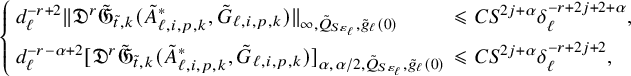 $$ \begin{align} \left\{ \begin{array}{ll} d_{\ell}^{-r+2} \|\mathfrak{D}^{r}\tilde{\mathfrak{G}}_{\tilde{t},k}(\tilde A_{\ell,i,p,k}^{*},\tilde G_{\ell,i,p,k})\|_{\infty,\tilde Q_{S\varepsilon_{\ell}},\tilde g_{\ell}(0)} &\leqslant CS^{2j+{\alpha}} \delta_{\ell}^{-r+2j+2+{\alpha}},\\[2mm] d_{\ell}^{-r-{\alpha}+2} [\mathfrak{D}^{r}\tilde{\mathfrak{G}}_{\tilde{t},k}(\tilde A_{\ell,i,p,k}^{*},\tilde G_{\ell,i,p,k})]_{{\alpha},{\alpha}/2,\tilde Q_{S\varepsilon_{\ell}},\tilde g_{\ell}(0)} &\leqslant CS^{2j+{\alpha}} \delta_{\ell}^{-r+2j+2}, \end{array} \right. \end{align} $$
for all
 $0\leqslant r\leqslant 2j+2$
and
$0\leqslant r\leqslant 2j+2$
and
 $S>1$
fixed.
$S>1$
fixed.
Next, we consider the case when
 $\varepsilon _{\ell }\leqslant C$
, and we take only derivatives and difference quotients in the base and time directions. The argument is similar to [Reference Hein and Tosatti21, (4.159)]. We start by noting that if a certain derivative
$\varepsilon _{\ell }\leqslant C$
, and we take only derivatives and difference quotients in the base and time directions. The argument is similar to [Reference Hein and Tosatti21, (4.159)]. We start by noting that if a certain derivative
 $\mathfrak {D}^\iota $
contains precisely u fiber derivatives (
$\mathfrak {D}^\iota $
contains precisely u fiber derivatives (
 $0\leqslant u\leqslant \iota $
), then we will denote it schematically by
$0\leqslant u\leqslant \iota $
), then we will denote it schematically by
![]() . We then have the easy bounds from [Reference Hein and Tosatti21, (4.153)–(4.154)]
. We then have the easy bounds from [Reference Hein and Tosatti21, (4.153)–(4.154)]
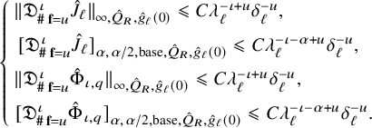
We use (4.162), (4.164) and (4.169) to obtain
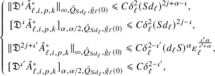 $$ \begin{align} \left\{ \begin{array}{ll} \|\mathfrak{D}^ \iota \hat A^{*}_{\ell,i,p,k}\|_{\infty,\hat Q_{Sd_{\ell}},\hat g_{\ell}(0)} \leqslant C\delta_{\ell}^2 (Sd_{\ell})^{2j+{\alpha}-\iota},\\[2mm] \, [\mathfrak{D}^ \iota \hat A^{*}_{\ell,i,p,k}]_{{\alpha},{\alpha}/2,\hat Q_{ Sd_{\ell}},\hat g_{\ell}(0)} \leqslant C\delta_{\ell}^2 (S d_{\ell})^{2j-\iota},\\[2mm] \|\mathfrak{D}^ {2j+\iota'} \hat A^{*}_{\ell,i,p,k}\|_{\infty,\hat Q_{Sd_{\ell}},\hat g_{\ell}(0)} \leqslant C\delta_{\ell}^{2-\iota'} (d_{\ell} S)^{\alpha} \varepsilon_{\ell}^{\frac{\iota' {\alpha}}{\iota'+{\alpha}}},\\[2mm] [\mathfrak{D}^{\iota'}\hat A_{\ell,i,p,k}^{*}]_{{\alpha},{\alpha}/2,\hat Q_{Sd_{\ell}},\hat g_{\ell}(0)}\leqslant C \delta_{\ell}^{2-\iota'}, \end{array} \right. \end{align} $$
for all
 $0\leqslant \iota \leqslant 2j$
,
$0\leqslant \iota \leqslant 2j$
,
 $1\leqslant \iota '\leqslant 2k+2$
and
$1\leqslant \iota '\leqslant 2k+2$
and
 $S>1$
fixed. Then (4.177), (4.182) and (4.183) imply
$S>1$
fixed. Then (4.177), (4.182) and (4.183) imply
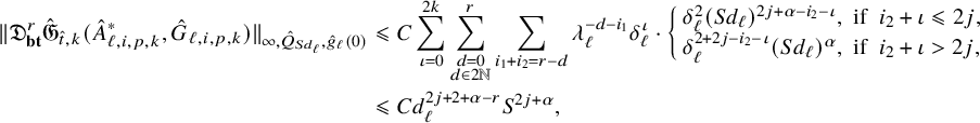 $$ \begin{align} \begin{aligned} \|\mathfrak{D}_{\textbf{bt}}^{r}\hat {\mathfrak{G}}_{\hat{t},k}(\hat A_{\ell,i,p,k}^{*},\hat G_{\ell,i,p,k})\|_{\infty,\hat Q_{Sd_{\ell}},\hat g_{\ell}(0)} &\leqslant C\sum_{\iota=0}^{2k} \sum_{\substack{d=0\\d\in 2\mathbb{N}}}^r \sum_{i_1+i_2=r-d} \lambda_{\ell}^{-d-i_1}\delta_{\ell}^{\iota }\cdot \left\{ \begin{array}{ll} \delta_{\ell}^2 (Sd_{\ell})^{2j+{\alpha}-i_2-\iota},\; \text{if}\;\; i_2+\iota \leqslant 2j,\\ \delta_{\ell}^{2+2j-i_2-\iota} (S d_{\ell} )^{\alpha} , \; \text{if}\;\; i_2+\iota> 2j,\\ \end{array} \right.\\ &\leqslant C d_{\ell}^{2j+2+{\alpha}-r}S^{2j+{\alpha}}, \end{aligned} \end{align} $$
for
 $0\leqslant r\leqslant 2j+2$
, and fixed
$0\leqslant r\leqslant 2j+2$
, and fixed
 $S>1$
. Arguing similarly for the Hölder seminorms, and transferring to the tilde picture yields
$S>1$
. Arguing similarly for the Hölder seminorms, and transferring to the tilde picture yields
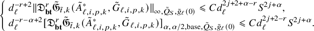 $$ \begin{align} \left\{\!\! \begin{array}{ll} & d_{\ell}^{-r+2}\|\mathfrak{D}_{\textbf{bt}}^{r}\tilde {\mathfrak{G}}_{\tilde{t},k}(\tilde A_{\ell,i,p,k}^{*},\tilde G_{\ell,i,p,k})\|_{\infty,\tilde Q_{S},\tilde g_{\ell}(0)}\leqslant C d_{\ell}^{2j+2+{\alpha}-r}S^{2j+{\alpha}}, \\ &d_{\ell}^{-r-{\alpha}+2}[\mathfrak{D}_{\textbf{bt}}^{r}\tilde {\mathfrak{G}}_{\tilde{t},k}(\tilde A_{\ell,i,p,k}^{*},\tilde G_{\ell,i,p,k})]_{{\alpha},{\alpha}/2,\mathrm{base},\tilde Q_{S},\tilde g_{\ell}(0)} \leqslant C d_{\ell}^{2j+2-r}S^{2j+{\alpha}}. \end{array} \right. \end{align} $$
Observe that when
 $r=2j+2$
, the leading term arises when
$r=2j+2$
, the leading term arises when
 $d=i_1=q=\iota =0$
and
$d=i_1=q=\iota =0$
and
 $i_2=2j+2$
, which in the tilde picture is given by
$i_2=2j+2$
, which in the tilde picture is given by
 $$ \begin{align} \mathfrak{D}_{\textbf{bt}}^{2j+2}\tilde {\mathfrak{G}}_{\tilde{t},k}(\tilde A_{\ell,i,p,k}^{*},\tilde G_{\ell,i,p,k}) =\sum_{i=1}^j \sum_{p=1}^{N_{i,k}} (\Delta_{\Theta_{\ell}^{*}\Psi_{\ell}^{*}\omega_{F}|_{ \{\cdot\}\times Y}})^{-1} \tilde G_{\ell,i,p,k} \cdot \mathfrak{D}^{2j+2}\tilde A_{\ell,i,p,k}^{*} +o(d_{\ell}^{2j+{\alpha}}). \end{align} $$
We now bound
 $\tilde \eta _{\ell }^\circ $
and its derivatives. Using [Reference Hein and Tosatti21, (4.139)], paying extra attention to the time derivatives, we have
$\tilde \eta _{\ell }^\circ $
and its derivatives. Using [Reference Hein and Tosatti21, (4.139)], paying extra attention to the time derivatives, we have
 $$ \begin{align} \kern-6pt\begin{aligned} \mathfrak{D}^r \hat\eta_{\ell}^\circ =\sum e^{-q(t_{\ell}+\lambda_{\ell}^{-2}\hat t)+\frac{\iota}{2}t_{\ell}} \left(q\lambda_{\ell}^{-2}\right)^{\frac{d}{2}}\delta_{\ell}^\iota (\mathfrak{D}^{r-d+1-s} \hat J_{\ell})\circledast \mathfrak{D}^{i_1}\hat \Phi_{\ell,\iota,q}(\hat G_{\ell,i,p,k}) \circledast \mathfrak{D}^{i_2+\iota} \hat A_{\ell,i,p,k}^{*}, \end{aligned} \end{align} $$
where
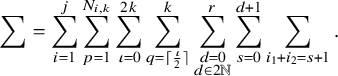 $$ \begin{align} \sum= \sum_{i=1}^j \sum_{p=1}^{N_{i,k}} \sum_{\iota=0}^{2k}\sum_{q=\lceil\frac{\iota}{2}\rceil}^{k}\sum_{\substack{d=0\\d\in 2\mathbb{N}}}^r \sum_{s=0}^{d+1}\sum_{i_1+i_2=s+1}. \end{align} $$
Using (4.176) with (4.178), we can estimate
 $\mathfrak {D}^r \hat \eta _{\ell }^\circ $
by
$\mathfrak {D}^r \hat \eta _{\ell }^\circ $
by
 $$ \begin{align} \begin{aligned} \|\mathfrak{D}^r \hat \eta_{\ell}^\circ\|_{\infty, \hat Q_{S\delta_{\ell}},\hat g_{\ell}(0)}&\leqslant CS^{2j+{\alpha}} \lambda_{\ell}^{-d} \delta_{\ell}^{\iota -r+d-1+s-i_1+2j+2+{\alpha}-i_2-\iota} \leqslant C S^{2j+{\alpha}} \delta_{\ell}^{ -r+2j+{\alpha}}, \end{aligned} \end{align} $$
where we have used the fact that
 $\delta _{\ell }= \lambda _{\ell } e^{-t_{\ell }/2}$
. Similarly,
$\delta _{\ell }= \lambda _{\ell } e^{-t_{\ell }/2}$
. Similarly,
In particular in the tilde picture,
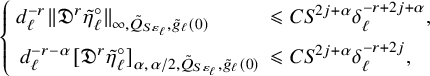 $$ \begin{align} \left\{ \begin{array}{ll} d_{\ell}^{-r}\|\mathfrak{D}^r\tilde \eta_{\ell}^\circ\|_{\infty, \tilde Q_{S\varepsilon_{\ell}},\tilde g_{\ell}(0)}& \leqslant C S^{2j+{\alpha}} \delta_{\ell}^{ -r+2j+{\alpha}},\\[2mm] \, d_{\ell}^{-r-{\alpha}}[\mathfrak{D}^r \tilde{\eta}_{\ell}^\circ]_{{\alpha},{\alpha}/2, \tilde Q_{S\varepsilon_{\ell}},\tilde g_{\ell}(0)}&\leqslant CS^{2j+{\alpha}} \delta_{\ell}^{ -r+2j}, \end{array} \right. \end{align} $$
for all
 $0\leqslant r\leqslant 2j$
(which is the analog of [Reference Hein and Tosatti21, (4.151)]).
$0\leqslant r\leqslant 2j$
(which is the analog of [Reference Hein and Tosatti21, (4.151)]).
These estimates are only useful when
 $\varepsilon _{\ell }\geqslant C^{-1}$
. In the case when
$\varepsilon _{\ell }\geqslant C^{-1}$
. In the case when
 $\varepsilon _{\ell }\to 0$
, we shall only take derivatives and difference quotients in the base and time directions. We can follow the argument to derive [Reference Hein and Tosatti21, (4.159)], using (4.162), (4.164),(4.166) and (4.167) instead of [Reference Hein and Tosatti21, (4.123), (4.125), (4.130)], and using
$\varepsilon _{\ell }\to 0$
, we shall only take derivatives and difference quotients in the base and time directions. We can follow the argument to derive [Reference Hein and Tosatti21, (4.159)], using (4.162), (4.164),(4.166) and (4.167) instead of [Reference Hein and Tosatti21, (4.123), (4.125), (4.130)], and using
 $\mathfrak {D}$
instead of
$\mathfrak {D}$
instead of
 ${\mathbb {D}}$
, and taking also time derivatives of
${\mathbb {D}}$
, and taking also time derivatives of
 $e^{-q(t_{\ell }+\lambda _{\ell }^{-2}\hat t)}$
in (4.187), we obtain
$e^{-q(t_{\ell }+\lambda _{\ell }^{-2}\hat t)}$
in (4.187), we obtain
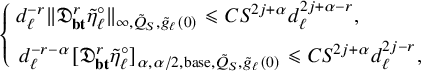 $$ \begin{align} \left\{ \begin{array}{ll} d_{\ell}^{-r}\|\mathfrak{D}_{\textbf{bt}}^r\tilde{\eta}_{\ell}^\circ \|_{\infty, \tilde Q_S,\tilde g_{\ell}(0)} \leqslant C S^{2j+{\alpha}} d_{\ell}^{2j+{\alpha}-r},\\[2mm] \, d_{\ell}^{-r-{\alpha}}[ \mathfrak{D}_{\textbf{bt}}^r\tilde{\eta}_{\ell}^\circ] _{{\alpha},{\alpha}/2,\mathrm{base}, \tilde Q_S,\tilde g_{\ell}(0)} \leqslant C S^{2j+{\alpha}} d_{\ell}^{2j-r},\\ \end{array} \right. \end{align} $$
for all
 $0\leqslant r\leqslant 2j$
and S fixed. Also, it is important to note that in the
$0\leqslant r\leqslant 2j$
and S fixed. Also, it is important to note that in the
 $L^\infty $
bound in (4.192) with
$L^\infty $
bound in (4.192) with
 $r=2j$
, which nominally is
$r=2j$
, which nominally is
 $O(d_{\ell }^{\alpha })$
, the only term which is not actually
$O(d_{\ell }^{\alpha })$
, the only term which is not actually
 $o(d_{\ell }^{\alpha })$
comes from the terms in the sum in (4.187) with
$o(d_{\ell }^{\alpha })$
comes from the terms in the sum in (4.187) with
 $d=0$
. To see this, we follow verbatim the discussion in [Reference Hein and Tosatti21, (4.161)], which gives us that
$d=0$
. To see this, we follow verbatim the discussion in [Reference Hein and Tosatti21, (4.161)], which gives us that
 $$ \begin{align} d_{\ell}^{-2j-{\alpha}} \mathfrak{D}_{\textbf{bt}}^{2j} \tilde \eta_{\ell}^\circ = d_{\ell}^{-2j-{\alpha}} \sum_{i=1}^j \sum_{p=1}^{N_{i,k}} \left({i\partial\bar\partial} (\Delta_{\Theta_{\ell}^{*}\Psi_{\ell}^{*}\omega_{F}|_{ \{\cdot\}\times Y}})^{-1} \tilde G_{\ell,i,p,k} \right)_{\textbf{ff}} \mathfrak{D}^{2j}\tilde A_{\ell,i,p,k}^{*} +o(1), \end{align} $$
locally uniformly.
Similarly, following the derivation of [Reference Hein and Tosatti21, (4.162)], in the case when
 $\varepsilon _{\ell }\to 0$
, we have
$\varepsilon _{\ell }\to 0$
, we have
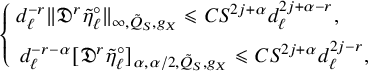 $$ \begin{align} \left\{ \begin{array}{ll} d_{\ell}^{-r} \| \mathfrak{D}^r \tilde{\eta}_{\ell}^\circ\|_{\infty,\tilde Q_S,g_X}\leqslant CS^{2j+{\alpha}} d_{\ell}^{2j+{\alpha}-r},\\[2mm] \, d_{\ell}^{-r-{\alpha}} [ \mathfrak{D}^r \tilde{\eta}_{\ell}^\circ]_{{\alpha},{\alpha}/2, \tilde Q_S,g_X}\leqslant CS^{2j+{\alpha}} d_{\ell}^{2j-r}, \end{array} \right. \end{align} $$
for all
 $0\leqslant r\leqslant 2j$
, fixed
$0\leqslant r\leqslant 2j$
, fixed
 $S>0$
and a fixed metric
$S>0$
and a fixed metric
 $g_X$
.
$g_X$
.
4.10.6 Estimates for
$\tilde {\eta }_{\ell }^\dagger $
and its potential

Recall that by definition we have
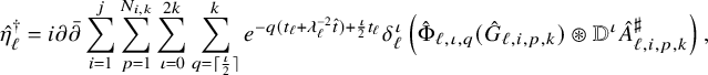 $$ \begin{align} \begin{aligned} \hat \eta_{\ell}^\dagger &= {i\partial\bar\partial} \sum_{i=1}^j \sum_{p=1}^{N_{i,k}} \sum_{\iota=0}^{2k}\sum_{q=\lceil\frac{\iota}{2}\rceil}^{k} e^{-q(t_{\ell}+\lambda_{\ell}^{-2}\hat t)+\frac{\iota}{2}t_{\ell}} \delta_{\ell}^\iota \left( \hat \Phi_{\ell,\iota,q}(\hat G_{\ell,i,p,k})\circledast {\mathbb{D}}^\iota \hat A_{\ell,i,p,k}^\sharp \right), \end{aligned} \end{align} $$
where we have applied (3.1). From (4.172), we have
 $$ \begin{align} \left\{ \begin{array}{ll} \|\mathfrak{D}^\iota \hat A_{\ell,i,p,k}^\sharp\|_{\infty,\hat Q_{S},\hat g_{\ell}(0)}\leqslant C \max( 1, S^{2j-\iota}) \delta_{\ell}^2 e^{\frac{-2i+2-{\alpha}}{2}\cdot \frac{{\alpha} }{2j+{\alpha}}t_{\ell}},\\ [2mm] \, [\mathfrak{D}^\iota \hat A_{\ell,i,p,k}^\sharp]_{{\beta},{\beta}/2,\hat Q_{S},\hat g_{\ell}(0)}\leqslant C \max( 1, S^{2j-\iota-{\beta}})\delta_{\ell}^2 e^{\frac{-2i+2-{\alpha}}{2}\cdot \frac{{\alpha} }{2j+{\alpha}}t_{\ell}}, \end{array} \right. \end{align} $$
for all
 $S>0$
,
$S>0$
,
 $0\leqslant \iota \leqslant 2j$
and
$0\leqslant \iota \leqslant 2j$
and
 $0<{\beta }<1$
, while the derivatives of (parabolic) order
$0<{\beta }<1$
, while the derivatives of (parabolic) order
 $>2j$
vanish since
$>2j$
vanish since
 $\hat A_{\ell ,i,p,k}^\sharp $
is a (parabolic) polynomial of degree at most
$\hat A_{\ell ,i,p,k}^\sharp $
is a (parabolic) polynomial of degree at most
 $2j$
. By applying
$2j$
. By applying
 $\mathfrak {D}^r$
to
$\mathfrak {D}^r$
to
 $\hat \eta _{\ell }^\dagger $
, we have
$\hat \eta _{\ell }^\dagger $
, we have
 $$ \begin{align} \begin{aligned} \mathfrak{D}^r \hat\eta_{\ell}^\dagger =\sum e^{-q(t_{\ell}+\lambda_{\ell}^{-2}\hat t)+\frac{\iota}{2}t_{\ell}} (q\lambda_{\ell}^{-2})^{\frac{d}{2}}\delta_{\ell}^\iota (\mathfrak{D}^{r-d+1-s} \hat J_{\ell})\circledast \mathfrak{D}^{i_1}\hat \Phi_{\iota,q}(\hat G_{\ell,i,p,k}) \circledast \mathfrak{D}^{i_2+\iota} \hat A_{\ell,i,p,k}^\sharp, \end{aligned} \end{align} $$
where
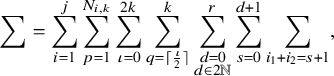 $$ \begin{align} \sum= \sum_{i=1}^j \sum_{p=1}^{N_{i,k}} \sum_{\iota=0}^{2k}\sum_{q=\lceil\frac{\iota}{2}\rceil}^{k}\sum_{\substack{d=0\\d\in 2\mathbb{N}}}^r \sum_{s=0}^{d+1}\sum_{i_1+i_2=s+1}, \end{align} $$
so that (4.176) and (4.196) imply
 $$ \begin{align} \begin{aligned} \|\mathfrak{D}^r \hat \eta_{\ell}^\dagger\|_{\infty,\hat Q_S,\hat g_{\ell}(0)} &\leqslant C\sum \lambda_{\ell}^{-d} \delta_{\ell}^{\iota -r+d-1+s-i_1+2}e^{\frac{-{\alpha}}{2}\cdot \frac{{\alpha} }{2j+{\alpha}}t_{\ell}}\leqslant C \delta_{\ell}^{-r}e^{\frac{-{\alpha}}{2}\cdot \frac{{\alpha} }{2j+{\alpha}}t_{\ell}}. \end{aligned} \end{align} $$
The Hölder seminorm is similar, and hence,
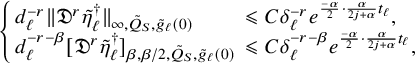 $$ \begin{align} \left\{ \begin{array}{ll} d_{\ell}^{-r} \|\mathfrak{D}^r \tilde{\eta}_{\ell}^\dagger\|_{\infty,\tilde Q_S,\tilde g_{\ell}(0)}&\leqslant C \delta_{\ell}^{-r}e^{\frac{-{\alpha}}{2}\cdot \frac{{\alpha} }{2j+{\alpha}}t_{\ell}},\\ d_{\ell}^{-r-{\beta}} [\mathfrak{D}^r \tilde{\eta}_{\ell}^\dagger]_{{\beta},{\beta}/2,\tilde Q_S,\tilde g_{\ell}(0)}&\leqslant C \delta_{\ell}^{-r-{\beta}} e^{\frac{-{\alpha}}{2}\cdot \frac{{\alpha} }{2j+{\alpha}}t_{\ell}}, \end{array} \right. \end{align} $$
for all
 $r\geqslant 0,{\beta }\in (0,1)$
and
$r\geqslant 0,{\beta }\in (0,1)$
and
 $S\leqslant Rd_{\ell }^{-1}$
with R fixed (as in [Reference Hein and Tosatti21, (4.172)]). Likewise, if we take at most 2 fiber derivatives landing on
$S\leqslant Rd_{\ell }^{-1}$
with R fixed (as in [Reference Hein and Tosatti21, (4.172)]). Likewise, if we take at most 2 fiber derivatives landing on
 $\hat \Phi $
and
$\hat \Phi $
and
 $\hat J_{\ell }$
, then we use (4.196) and (4.182) to get
$\hat J_{\ell }$
, then we use (4.196) and (4.182) to get
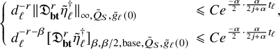 $$ \begin{align} \left\{ \begin{array}{ll} d_{\ell}^{-r} \|\mathfrak{D}^r_{\textbf{bt}} \tilde{\eta}_{\ell}^\dagger\|_{\infty,\tilde Q_S,\tilde g_{\ell}(0)}&\leqslant C e^{\frac{-{\alpha}}{2}\cdot \frac{{\alpha} }{2j+{\alpha}}t_{\ell}},\\[2mm] d_{\ell}^{-r-{\beta}} [\mathfrak{D}^r_{\textbf{bt}} \tilde{\eta}_{\ell}^\dagger]_{{\beta},{\beta}/2,\mathrm{base} ,\tilde Q_S,\tilde g_{\ell}(0)}&\leqslant C e^{\frac{-{\alpha}}{2}\cdot \frac{{\alpha} }{2j+{\alpha}}t_{\ell}} \end{array} \right. \end{align} $$
for all
 $r\geqslant 0,{\beta }\in (0,1)$
and
$r\geqslant 0,{\beta }\in (0,1)$
and
 $S\leqslant Rd_{\ell }^{-1}$
with R fixed (as in [Reference Hein and Tosatti21, (4.173)]). In particular, they converge to zero. If instead we use fixed metric
$S\leqslant Rd_{\ell }^{-1}$
with R fixed (as in [Reference Hein and Tosatti21, (4.173)]). In particular, they converge to zero. If instead we use fixed metric
 $g_X$
, then the derivatives of
$g_X$
, then the derivatives of
 $\hat \Phi $
and
$\hat \Phi $
and
 $\hat J_{\ell }$
are bounded, and thus,
$\hat J_{\ell }$
are bounded, and thus,
 $$ \begin{align} \left\{ \begin{array}{ll} \|\mathfrak{D}^r \hat\eta_{\ell}^\dagger\|_{\infty,\hat Q_S,g_X}&\leqslant C \delta_{\ell}^{2}e^{\frac{-{\alpha}}{2}\cdot \frac{{\alpha} }{2j+{\alpha}}t_{\ell}},\\[2mm] \, [\mathfrak{D}^r \hat\eta_{\ell}^\dagger]_{{\beta},{\beta}/2,\hat Q_S,g_X}&\leqslant C \delta_{\ell}^{2} e^{\frac{-{\alpha}}{2}\cdot \frac{{\alpha} }{2j+{\alpha}}t_{\ell}}, \end{array} \right. \end{align} $$
for all
 $r\geqslant 0,{\beta }\in (0,1)$
and fixed
$r\geqslant 0,{\beta }\in (0,1)$
and fixed
 $S>0$
(as in [Reference Hein and Tosatti21, (4.174)]). Similarly to the discussion of [Reference Hein and Tosatti21, (4.175)], we also have
$S>0$
(as in [Reference Hein and Tosatti21, (4.174)]). Similarly to the discussion of [Reference Hein and Tosatti21, (4.175)], we also have
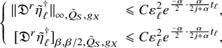 $$ \begin{align} \left\{ \begin{array}{ll} \|\mathfrak{D}^r \tilde{\eta}_{\ell}^\dagger\|_{\infty,\tilde Q_S,g_X}&\leqslant C \varepsilon_{\ell}^{2}e^{\frac{-{\alpha}}{2}\cdot \frac{{\alpha} }{2j+{\alpha}}t_{\ell}},\\[2mm] \, [\mathfrak{D}^r \tilde{\eta}_{\ell}^\dagger]_{{\beta},{\beta}/2,\tilde Q_S,g_X}&\leqslant C \varepsilon_{\ell}^{2} e^{\frac{-{\alpha}}{2}\cdot \frac{{\alpha} }{2j+{\alpha}}t_{\ell}}, \end{array} \right. \end{align} $$
for all
 $r\geqslant 0,{\beta }\in (0,1)$
and fixed
$r\geqslant 0,{\beta }\in (0,1)$
and fixed
 $S>0$
(as in [Reference Hein and Tosatti21, (4.175)]).
$S>0$
(as in [Reference Hein and Tosatti21, (4.175)]).
Next, we estimate the potential of
 $\tilde {\eta }_{\ell }^\dagger $
when
$\tilde {\eta }_{\ell }^\dagger $
when
 $\varepsilon _{\ell }\leqslant C$
. Given
$\varepsilon _{\ell }\leqslant C$
. Given
 $r\geqslant 0$
, by applying
$r\geqslant 0$
, by applying
 $\mathfrak {D}^r_{\textbf {bt}}$
to
$\mathfrak {D}^r_{\textbf {bt}}$
to
 $ \hat {\mathfrak {G}}_{\hat {t},k}(\hat A_{\ell ,i,p,k}^\sharp ,\hat G_{\ell ,i,p,k})$
with (3.1)
$ \hat {\mathfrak {G}}_{\hat {t},k}(\hat A_{\ell ,i,p,k}^\sharp ,\hat G_{\ell ,i,p,k})$
with (3.1)
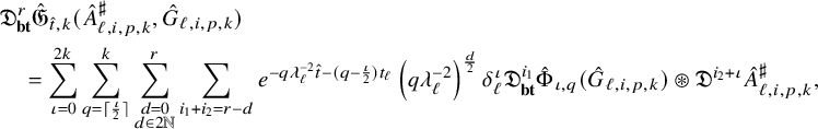 $$ \begin{align} \begin{aligned} &\mathfrak{D}^r_{\textbf{bt}}\hat{\mathfrak{G}}_{\hat{t},k}(\hat A_{\ell,i,p,k}^\sharp,\hat G_{\ell,i,p,k})\\ &\quad= \sum_{\iota=0}^{2k}\sum_{q=\lceil\frac{\iota}{2}\rceil}^{k} \sum_{\substack{d=0\\d\in 2\mathbb{N}}}^r \sum_{i_1+i_2=r-d}e^{-q\lambda_{\ell}^{-2}\hat t-(q-\frac{\iota}{2})t_{\ell}} \left(q\lambda_{\ell}^{-2}\right)^{\frac{d}{2}} \delta_{\ell}^\iota\mathfrak{D}_{\textbf{bt}}^{i_1}\hat \Phi_{\iota,q}(\hat G_{\ell,i,p,k}) \circledast \mathfrak{D}^{i_2+\iota} \hat A_{\ell,i,p,k}^\sharp, \end{aligned} \end{align} $$
which can be estimated using (4.196) and (4.182) to get
 $$ \begin{align} \begin{aligned} [ \mathfrak{D}^r_{\textbf{bt}}\hat{\mathfrak{G}}_{\hat{t},k}(\hat A_{\ell,i,p,k}^\sharp,\hat G_{\ell,i,p,k})]_{{\alpha},{\alpha}/2,\mathrm{base},\hat Q_{S d_{\ell}},\hat g_{\ell}(0)}\leqslant C \sum_{\iota=0}^{2k} \sum_{\substack{d=0\\d\in 2\mathbb{N}}}^r \sum_{i_1+i_2=r-d}\lambda_{\ell}^{-d-i_1}\delta_{\ell}^{\iota+2} e^{\frac{-2i+2-{\alpha}}{2}\cdot \frac{{\alpha} }{2j+{\alpha}}t_{\ell}}=o(1). \end{aligned} \end{align} $$
The
 $L^\infty $
norm is similar, and hence in the tilde picture we have
$L^\infty $
norm is similar, and hence in the tilde picture we have
 $$ \begin{align} \left\{ \begin{array}{ll} d_{\ell}^{-r+2-{\alpha}}[ \mathfrak{D}^{r}_{\textbf{bt}}\tilde{\mathfrak{G}}_{\tilde{t},k}(\tilde A_{\ell,i,p,k}^\sharp,\tilde G_{\ell,i,p,k})]_{{\alpha},{\alpha}/2,\mathrm{base},\tilde Q_{S},\tilde g_{\ell}(0)}=o(1),\\[2mm] d_{\ell}^{-r+2}\| \mathfrak{D}^{r}_{\textbf{bt}}\tilde{\mathfrak{G}}_{\tilde{t},k}(\tilde A_{\ell,i,p,k}^\sharp,\tilde G_{\ell,i,p,k})\|_{\infty,\tilde Q_{S},\tilde g_{\ell}(0)}=o(1),\\[2mm] \end{array} \right. \end{align} $$
for all
 $r\geqslant 0$
and S fixed.
$r\geqslant 0$
and S fixed.
4.10.7 Estimates for
$\tilde {\omega }_{\ell }^\sharp $

Recall that
 $$ \begin{align} \tilde{\omega}_{\ell}^\sharp(\tilde t)=(1-e^{-t_{\ell}-d_{\ell}^2\lambda_{\ell}^{-2}\tilde t})\tilde{\omega}_{\ell,\mathrm{can}}+\varepsilon_{\ell}^2 e^{-d_{\ell}^2\lambda_{\ell}^{-2}\tilde t}\Theta_{\ell}^{*}\Psi_{\ell}^{*}\omega_{F} +\tilde{\eta}_{\ell}^\dagger+\tilde{\eta}_{\ell}^\ddagger. \end{align} $$
We can follow exactly the same discussion in [Reference Hein and Tosatti21, §4.9.7] to conclude the following. Since
 $\tilde {\omega }_{\ell ,\mathrm {can}}=d_{\ell }^{-2}\lambda _{\ell }^2\Theta _{\ell }^{*}\Psi _{\ell }^{*} \omega _{\mathrm {can}}$
and
$\tilde {\omega }_{\ell ,\mathrm {can}}=d_{\ell }^{-2}\lambda _{\ell }^2\Theta _{\ell }^{*}\Psi _{\ell }^{*} \omega _{\mathrm {can}}$
and
 $(\Psi _{\ell } \circ \Theta _{\ell })(\tilde z,\tilde y)=(d_{\ell } \lambda _{\ell }^{-1}z,y)$
where
$(\Psi _{\ell } \circ \Theta _{\ell })(\tilde z,\tilde y)=(d_{\ell } \lambda _{\ell }^{-1}z,y)$
where
 $d_{\ell } \lambda _{\ell }^{-1}\to 0$
, the spatial stretching implies
$d_{\ell } \lambda _{\ell }^{-1}\to 0$
, the spatial stretching implies
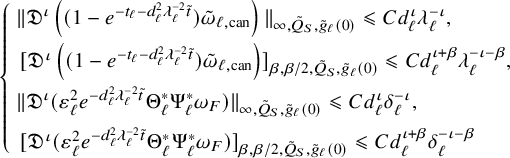 $$ \begin{align} \left\{ \begin{array}{ll} \| \mathfrak{D}^{\iota} \left((1-e^{-t_{\ell}-d_{\ell}^2\lambda_{\ell}^{-2}\tilde t})\tilde{\omega}_{\ell,\mathrm{can}}\right)\|_{\infty,\tilde Q_{S},\tilde g_{\ell}(0)}\leqslant C d_{\ell}^\iota \lambda_{\ell}^{-\iota},\\[2mm] \,[ \mathfrak{D}^{\iota}\left((1-e^{-t_{\ell}-d_{\ell}^2\lambda_{\ell}^{-2}\tilde t})\tilde{\omega}_{\ell,\mathrm{can}}\right)]_{{\beta},{\beta}/2,\tilde Q_{S},\tilde g_{\ell}(0)}\leqslant C d_{\ell}^{\iota+{\beta}} \lambda_{\ell}^{-\iota-{\beta}},\\[2mm] \| \mathfrak{D}^{\iota} (\varepsilon_{\ell}^2 e^{-d_{\ell}^2\lambda_{\ell}^{-2}\tilde t}\Theta_{\ell}^{*}\Psi_{\ell}^{*}\omega_F ) \|_{\infty,\tilde Q_{S},\tilde g_{\ell}(0)}\leqslant C d_{\ell}^\iota \delta_{\ell}^{-\iota},\\[2mm] \, [\mathfrak{D}^{\iota} (\varepsilon_{\ell}^2 e^{-d_{\ell}^2\lambda_{\ell}^{-2}\tilde t}\Theta_{\ell}^{*}\Psi_{\ell}^{*}\omega_F ) ]_{{\beta},{\beta}/2,\tilde Q_{S},\tilde g_{\ell}(0)}\leqslant C d_{\ell}^{\iota+{\beta}} \delta_{\ell}^{-\iota-{\beta}} \end{array} \right. \end{align} $$
for all
 $\iota \geqslant 0,{\beta }\in (0,1)$
and
$\iota \geqslant 0,{\beta }\in (0,1)$
and
 $S\leqslant Rd_{\ell }^{-1}$
with R fixed (which is the analog [Reference Hein and Tosatti21, (4.181)–(4.182)]). Therefore,
$S\leqslant Rd_{\ell }^{-1}$
with R fixed (which is the analog [Reference Hein and Tosatti21, (4.181)–(4.182)]). Therefore,
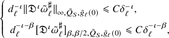 $$ \begin{align} \left\{ \begin{array}{ll} d_{\ell}^{-\iota} \|\mathfrak{D}^\iota \tilde{\omega}_{\ell}^\sharp\|_{\infty,\tilde Q_S,\tilde g_{\ell}(0)} \leqslant C\delta_{\ell}^{-\iota},\\[2mm] \, d_{\ell}^{-\iota-{\beta}} [\mathfrak{D}^\iota \tilde{\omega}_{\ell}^\sharp]_{{\beta},{\beta}/2,\tilde Q_S,\tilde g_{\ell}(0)} \leqslant C\delta_{\ell}^{-\iota-{\beta}}, \end{array} \right. \end{align} $$
for all
 $\iota \geqslant 0,{\beta }\in (0,1)$
and
$\iota \geqslant 0,{\beta }\in (0,1)$
and
 $S\leqslant Rd_{\ell }^{-1}$
with R fixed. Likewise, if we only differentiate in the base and time directions, then we have the following improvement:
$S\leqslant Rd_{\ell }^{-1}$
with R fixed. Likewise, if we only differentiate in the base and time directions, then we have the following improvement:
 $$ \begin{align} \left\{ \begin{array}{ll} d_{\ell}^{-\iota} \|\mathfrak{D}^\iota_{\textbf{bt}} \tilde{\omega}_{\ell}^\sharp\|_{\infty,\tilde Q_S,\tilde g_{\ell}(0)}=o(1),\\[2mm] \, d_{\ell}^{-\iota-{\beta}} [\mathfrak{D}^\iota_{\textbf{bt}} \tilde{\omega}_{\ell}^\sharp]_{{\beta},{\beta}/2,\mathrm{base},\tilde Q_S,\tilde g_{\ell}(0)} =o(1), \end{array} \right. \end{align} $$
for all
 $\iota \geqslant 0,{\beta }\in (0,1)$
with
$\iota \geqslant 0,{\beta }\in (0,1)$
with
 $\iota +{\beta }>0$
and
$\iota +{\beta }>0$
and
 $S\leqslant C d_{\ell }^{-1}$
(which is the analog of [Reference Hein and Tosatti21, (4.183)]) as well as
$S\leqslant C d_{\ell }^{-1}$
(which is the analog of [Reference Hein and Tosatti21, (4.183)]) as well as
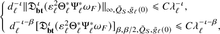 $$ \begin{align} \left\{ \begin{array}{ll} d_{\ell}^{-\iota} \|\mathfrak{D}^\iota_{\textbf{bt}} (\varepsilon_{\ell}^2 \Theta_{\ell}^{*}\Psi_{\ell}^{*} \omega_F)\|_{\infty,\tilde Q_S,\tilde g_{\ell}(0)}\leqslant C \lambda_{\ell}^{-\iota},\\[2mm] \, d_{\ell}^{-\iota-{\beta}} [\mathfrak{D}^\iota_{\textbf{bt}} (\varepsilon_{\ell}^2 \Theta_{\ell}^{*}\Psi_{\ell}^{*} \omega_F)]_{{\beta},{\beta}/2,\tilde Q_S,\tilde g_{\ell}(0)}\leqslant C \lambda_{\ell}^{-\iota-{\beta}}, \end{array} \right. \end{align} $$
for all
 $\iota \geqslant 0,{\beta }\in (0,1)$
and
$\iota \geqslant 0,{\beta }\in (0,1)$
and
 $S\leqslant C d_{\ell }^{-1}$
(which is the analog of [Reference Hein and Tosatti21, (4.184)–(4.185)])
$S\leqslant C d_{\ell }^{-1}$
(which is the analog of [Reference Hein and Tosatti21, (4.184)–(4.185)])
4.11 Expansion of the Monge-Ampère flow
We rewrite the complex Monge-Ampère equation (4.107) as
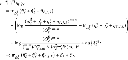 $$ \begin{align} \begin{aligned} &e^{-d_{\ell}^2\lambda_{\ell}^{-2}\tilde t} \partial_{\tilde t}\tilde \chi_{\ell}\\& \quad = \operatorname{tr}_{\tilde \omega_{\ell}^\sharp}\left(\tilde{\eta}_{\ell}^\circ+\tilde{\eta}_{\ell}^\diamondsuit+\tilde{\eta}_{\ell,j,k}\right) \\&\qquad+\left( \log \frac{(\tilde \omega_{\ell}^\sharp +\tilde{\eta}_{\ell}^\circ+\tilde{\eta}_{\ell}^\diamondsuit+\tilde{\eta}_{\ell,j,k})^{m+n}}{ (\tilde{\omega}_{\ell}^\sharp)^{m+n}}-\operatorname{tr}_{\tilde \omega_{\ell}^\sharp}\left(\tilde{\eta}_{\ell}^\circ+\tilde{\eta}_{\ell}^\diamondsuit+\tilde{\eta}_{\ell,j,k}\right)\right) \\&\qquad +\log \frac{(\tilde{\omega}_{\ell}^\sharp)^{m+n}}{ \binom{m+n}{m}\tilde \omega_{\ell,\mathrm{can}} ^m \wedge (\varepsilon_{\ell}^2 \Theta_{\ell}^{*}\Psi_{\ell}^{*} \omega_F)^n}+nd_{\ell}^2\lambda_{\ell}^{-2}\tilde t\\& \quad =:\operatorname{tr}_{\tilde \omega_{\ell}^\sharp}\left(\tilde{\eta}_{\ell}^\circ+\tilde{\eta}_{\ell}^\diamondsuit+\tilde{\eta}_{\ell,j,k}\right) +\mathcal{E}_1+\mathcal{E}_2, \end{aligned} \end{align} $$
where the terms
 $\mathcal {E}_1$
and
$\mathcal {E}_1$
and
 $\mathcal {E}_2$
are given respectively by the third and second line from the bottom in (4.212). Recall also that
$\mathcal {E}_2$
are given respectively by the third and second line from the bottom in (4.212). Recall also that
 $$ \begin{align} \begin{aligned} \tilde \chi_{\ell}=e^{d_{\ell}^2\lambda_{\ell}^{-2}\tilde t} \left(\tilde \psi_{\ell,j,k}+ \sum_{i=1}^j\sum_{p=1}^{N_{i,k}} \tilde{\mathfrak{G}}_{\tilde{t},k}( \tilde A_{\ell,i,p,k}^{*},\tilde G_{\ell,i,p,k} )\right)+ e^{d_{\ell}^2\lambda_{\ell}^{-2}\tilde t} \sum_{i=1}^j\sum_{p=1}^{N_{i,k}} \tilde{\mathfrak{G}}_{\tilde{t},k}( \tilde A_{\ell,i,p,k}^\sharp,\tilde G_{\ell,i,p,k} )+\underline{\tilde{\chi}_{\ell}^{*}}+\underline{\tilde{\chi}_{\ell}^\sharp} \end{aligned} \end{align} $$
so that if we define
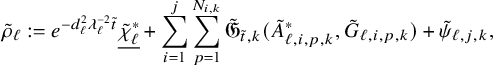 $$ \begin{align} \tilde{\rho}_{\ell}:=e^{-d_{\ell}^2\lambda_{\ell}^{-2}\tilde t}\underline{\tilde{\chi}_{\ell}^{*}}+\sum_{i=1}^j\sum_{p=1}^{N_{i,k}} \tilde{\mathfrak{G}}_{\tilde{t},k}( \tilde A_{\ell,i,p,k}^{*},\tilde G_{\ell,i,p,k} )+\tilde \psi_{\ell,j,k}, \end{align} $$
then by definition, we have
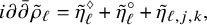 $$ \begin{align} {i\partial\bar\partial}\tilde{\rho}_{\ell}=\tilde{\eta}_{\ell}^\diamondsuit+ \tilde{\eta}_{\ell}^\circ+\tilde{\eta}_{\ell,j,k}, \end{align} $$
and we can further rewrite the (4.212) as
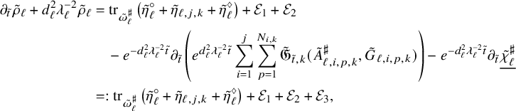 $$ \begin{align} \begin{aligned} \partial_{\tilde t} \tilde{\rho}_{\ell}+d_{\ell}^2\lambda_{\ell}^{-2}\tilde{\rho}_{\ell}&=\operatorname{tr}_{\tilde \omega_{\ell}^\sharp}\left(\tilde{\eta}_{\ell}^\circ+\tilde{\eta}_{\ell,j,k}+\tilde{\eta}_{\ell}^\diamondsuit\right) +\mathcal{E}_1+\mathcal{E}_2\\ &\quad - e^{-d_{\ell}^2\lambda_{\ell}^{-2}\tilde t}\partial_{\tilde t} \left( e^{d_{\ell}^2\lambda_{\ell}^{-2}\tilde t} \sum_{i=1}^j\sum_{p=1}^{N_{i,k}} \tilde{\mathfrak{G}}_{\tilde{t},k}( \tilde A_{\ell,i,p,k}^\sharp,\tilde G_{\ell,i,p,k} )\right)-e^{-d_{\ell}^2\lambda_{\ell}^{-2}\tilde t}\partial_{\tilde t}\underline{\tilde{\chi}_{\ell}^\sharp}\\ &=:\operatorname{tr}_{\tilde \omega_{\ell}^\sharp}\left(\tilde{\eta}_{\ell}^\circ+\tilde{\eta}_{\ell,j,k}+\tilde{\eta}_{\ell}^\diamondsuit\right) +\mathcal{E}_1+\mathcal{E}_2+\mathcal{E}_3, \end{aligned} \end{align} $$
where we defined
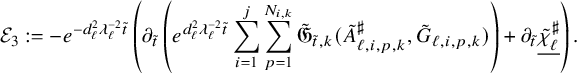 $$ \begin{align} \mathcal{E}_3:=- e^{-d_{\ell}^2\lambda_{\ell}^{-2}\tilde t}\left(\partial_{\tilde t} \left( e^{d_{\ell}^2\lambda_{\ell}^{-2}\tilde t} \sum_{i=1}^j\sum_{p=1}^{N_{i,k}} \tilde{\mathfrak{G}}_{\tilde{t},k}( \tilde A_{\ell,i,p,k}^\sharp,\tilde G_{\ell,i,p,k} )\right)+\partial_{\tilde t}\underline{\tilde{\chi}_{\ell}^\sharp}\right). \end{align} $$
The next Proposition gives us control on the error terms
 $\mathcal {E}_i$
:
$\mathcal {E}_i$
:
Proposition 4.7. For any fixed
 $R>0$
and
$R>0$
and
 $i=1,2,3$
, we have
$i=1,2,3$
, we have
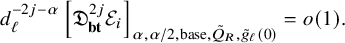 $$ \begin{align} d_{\ell}^{-2j-{\alpha}} \left[\mathfrak{D}^{2j}_{\textbf{bt}} \mathcal{E}_i \right]_{{\alpha},{\alpha}/2,\mathrm{base},\tilde Q_R,\tilde g_{\ell}(0)}=o(1). \end{align} $$
In particular,
 $$ \begin{align} \begin{aligned} d_{\ell}^{-2j-{\alpha}}&\Bigg[ \mathfrak{D}^{2j}_{\textbf{bt}}\bigg(\partial_{\tilde t} \tilde{\rho}_{\ell}+d_{\ell}^2\lambda_{\ell}^{-2}\tilde{\rho}_{\ell} - \operatorname{tr}_{\tilde \omega_{\ell}^\sharp}\left(\tilde{\eta}_{\ell}^\diamondsuit+ \tilde{\eta}_{\ell}^\circ+\tilde{\eta}_{\ell,j,k}\right) \bigg)\Bigg]_{{\alpha},{\alpha}/2,\mathrm{base},\tilde Q_R,\tilde g_{\ell}(0)}=o(1). \end{aligned} \end{align} $$
Furthermore, if
 $\varepsilon _{\ell }\geqslant C^{-1}$
, then for any fixed
$\varepsilon _{\ell }\geqslant C^{-1}$
, then for any fixed
 $R>1$
and
$R>1$
and
 $0\leqslant a\leqslant 2j$
, we have
$0\leqslant a\leqslant 2j$
, we have
 $$ \begin{align} d_{\ell}^{-2j-{\alpha}}\|\mathfrak{D}^a\mathcal{E}_1\|_{\infty,\tilde Q_{R\varepsilon_{\ell}}, \tilde g_{\ell}(0)}\leqslant C\delta_{\ell}^{2j+{\alpha} } \varepsilon_{\ell}^{2j+{\alpha}-a}, \end{align} $$
 $$ \begin{align} d_{\ell}^{-2j-{\alpha}}[\mathfrak{D}^a\mathcal{E}_1]_{{\alpha},{\alpha}/2,\tilde Q_{R\varepsilon_{\ell}}, \tilde g_{\ell}(0)}\leqslant C\delta_{\ell}^{2j+{\alpha} } \varepsilon_{\ell}^{2j-a}, \end{align} $$
 $$ \begin{align} d_{\ell}^{-2j-{\alpha}}\|\mathfrak{D}^a (\mathcal{E}_2+\mathcal{E}_3)\|_{\infty,\tilde Q_{R\varepsilon_{\ell}}, \tilde g_{\ell}(0)}\leqslant C\varepsilon_{\ell}^{2j+{\alpha}-a}, \end{align} $$
 $$ \begin{align} d_{\ell}^{-2j-{\alpha}}[ \mathfrak{D}^a(\mathcal{E}_2+\mathcal{E}_3)]_{{\alpha},{\alpha}/2,\tilde Q_{R\varepsilon_{\ell}}, \tilde g_{\ell}(0)}\leqslant C\varepsilon_{\ell}^{2j-a}. \end{align} $$
Proof. The estimate (4.218) for
 $\mathcal {E}_3$
follows easily from (4.158) and (4.206).
$\mathcal {E}_3$
follows easily from (4.158) and (4.206).
As for
 $\mathcal {E}_2$
, recall that
$\mathcal {E}_2$
, recall that
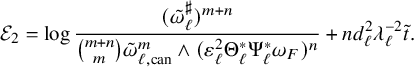 $$ \begin{align} \begin{aligned} \mathcal{E}_2&=\log \frac{(\tilde{\omega}_{\ell}^\sharp)^{m+n}}{ \binom{m+n}{m}\tilde{\omega}_{\ell,\mathrm{can}}^m\wedge (\varepsilon_{\ell}^2 \Theta_{\ell}^{*}\Psi_{\ell}^{*}\omega_{F})^n }+nd_{\ell}^2\lambda_{\ell}^{-2}\tilde t. \end{aligned} \end{align} $$
The term
 $nd_{\ell }^2\lambda _{\ell }^{-2}\tilde t$
is killed by
$nd_{\ell }^2\lambda _{\ell }^{-2}\tilde t$
is killed by
 $[\mathfrak {D}_{\textbf {bt}}^{2j}\cdot ]_{{\alpha },{\alpha }/2,\mathrm {base}}$
if
$[\mathfrak {D}_{\textbf {bt}}^{2j}\cdot ]_{{\alpha },{\alpha }/2,\mathrm {base}}$
if
 $j>0$
, while if
$j>0$
, while if
 $j=0$
, we have
$j=0$
, we have
 $$ \begin{align} d_{\ell}^{-\alpha}[nd_{\ell}^2\lambda_{\ell}^{-2}\tilde t]_{{\alpha},{\alpha}/2,\mathrm{base},\tilde Q_R,\tilde g_{\ell}(0)}\leqslant Cd_{\ell}^{2-\alpha}\lambda_{\ell}^{-2}=o(1). \end{align} $$
Estimate (4.218) for
 $\mathcal {E}_2$
then follows from this together with (4.208), (4.210) and (4.211).
$\mathcal {E}_2$
then follows from this together with (4.208), (4.210) and (4.211).
For
 $\mathcal {E}_1$
, we write
$\mathcal {E}_1$
, we write
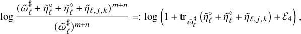 $$ \begin{align} \begin{aligned} &\quad \log \frac{(\tilde \omega_{\ell}^\sharp +\tilde{\eta}_{\ell}^\circ+\tilde{\eta}_{\ell}^\diamondsuit+\tilde{\eta}_{\ell,j,k})^{m+n}}{ (\tilde{\omega}_{\ell}^\sharp)^{m+n}}=:\log \left( 1+\operatorname{tr}_{\tilde \omega_{\ell}^\sharp}\left(\tilde{\eta}_{\ell}^\circ+\tilde{\eta}_{\ell}^\diamondsuit+\tilde{\eta}_{\ell,j,k}\right) +\mathcal{E}_4\right), \end{aligned} \end{align} $$
where we defined
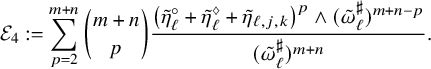 $$ \begin{align} \mathcal{E}_4:=\sum_{p=2}^{m+n}\binom{m+n}{p}\frac{\left(\tilde{\eta}_{\ell}^\circ+\tilde{\eta}_{\ell}^\diamondsuit+\tilde{\eta}_{\ell,j,k}\right)^p\wedge(\tilde \omega_{\ell}^\sharp)^{m+n-p}}{(\tilde \omega_{\ell}^\sharp)^{m+n}}. \end{align} $$
Thanks to (4.145), (4.159), (4.192) and (4.210), for every
 $0\leqslant \iota \leqslant 2j$
and fixed
$0\leqslant \iota \leqslant 2j$
and fixed
 $R>0$
, we have
$R>0$
, we have
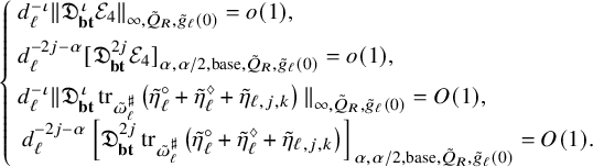 $$ \begin{align} \left\{ \begin{array}{ll} d_{\ell}^{-\iota}\|\mathfrak{D}^{\iota}_{\textbf{bt}}\mathcal{E}_4\|_{\infty,\tilde Q_R, \tilde g_{\ell}(0)}=o(1),\\[2mm] d_{\ell}^{-2j-{\alpha}}[\mathfrak{D}^{2j}_{\textbf{bt}}\mathcal{E}_4]_{{\alpha},{\alpha}/2,\mathrm{base},\tilde Q_R, \tilde g_{\ell}(0)}=o(1),\\[2mm] d_{\ell}^{-\iota}\|\mathfrak{D}_{\textbf{bt}}^\iota \operatorname{tr}_{\tilde \omega_{\ell}^\sharp}\left(\tilde{\eta}_{\ell}^\circ+\tilde{\eta}_{\ell}^\diamondsuit+\tilde{\eta}_{\ell,j,k}\right)\|_{\infty,\tilde Q_R,\tilde g_{\ell}(0)}=O(1),\\ \, d_{\ell}^{-2j-{\alpha}}\left [\mathfrak{D}^{2j}_{\textbf{bt}}\operatorname{tr}_{\tilde \omega_{\ell}^\sharp}\left(\tilde{\eta}_{\ell}^\circ+\tilde{\eta}_{\ell}^\diamondsuit+\tilde{\eta}_{\ell,j,k}\right)\right]_{{\alpha},{\alpha}/2,\mathrm{base},\tilde Q_R,\tilde g_{\ell}(0)}=O(1).\\ \end{array} \right. \end{align} $$
If we write schematically
 $\mathbf {A}=\operatorname {tr}_{\tilde \omega _{\ell }^\sharp }\left(\tilde {\eta }_{\ell }^\circ +\tilde {\eta }_{\ell }^\diamondsuit +\tilde {\eta }_{\ell ,j,k}\right), \mathbf {B}=\mathcal {E}_4$
, which are both
$\mathbf {A}=\operatorname {tr}_{\tilde \omega _{\ell }^\sharp }\left(\tilde {\eta }_{\ell }^\circ +\tilde {\eta }_{\ell }^\diamondsuit +\tilde {\eta }_{\ell ,j,k}\right), \mathbf {B}=\mathcal {E}_4$
, which are both
 $o(1)$
locally uniformly, then we have
$o(1)$
locally uniformly, then we have
 $\mathcal {E}_1=\log (1+\mathbf {A}+\mathbf {B})-\mathbf {A}.$
For any
$\mathcal {E}_1=\log (1+\mathbf {A}+\mathbf {B})-\mathbf {A}.$
For any
 $a\geqslant 0$
, we can then write schematically
$a\geqslant 0$
, we can then write schematically
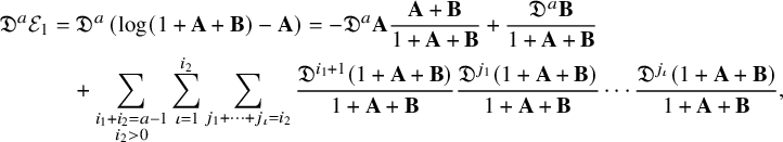 $$ \begin{align} \begin{aligned} \mathfrak{D}^a\mathcal{E}_1&=\mathfrak{D}^a \left(\log (1+\mathbf{A}+\mathbf{B})-\mathbf{A} \right) =-\mathfrak{D}^a\mathbf{A}\frac{\mathbf{A}+\mathbf{B}}{1+\mathbf{A}+\mathbf{B}}+\frac{\mathfrak{D}^a\mathbf{B}}{1+\mathbf{A}+\mathbf{B}}\\& \quad +\sum_{\substack{i_1+i_2=a-1\\ i_2>0}}\sum_{\iota=1}^{i_2}\sum_{j_1+\dots+j_{\iota}=i_2} \frac{\mathfrak{D}^{i_1+1}(1+\mathbf{A}+\mathbf{B})}{1+\mathbf{A}+\mathbf{B}} \frac{\mathfrak{D}^{j_1}(1+\mathbf{A}+\mathbf{B})}{1+\mathbf{A}+\mathbf{B}}\cdots \frac{\mathfrak{D}^{j_\iota}(1+\mathbf{A}+\mathbf{B})}{1+\mathbf{A}+\mathbf{B}}, \end{aligned} \end{align} $$
and then (4.218) for
 $\mathcal {E}_1$
follows from (4.228).
$\mathcal {E}_1$
follows from (4.228).
Now that (4.218) is established, (4.219) follows immediately from this and (4.216).
When
 $\varepsilon _{\ell } \geqslant C^{-1}$
, estimates (4.220) and (4.221) follow from (4.145), (4.159), (4.191), (4.209) together with (4.229). Lastly, to prove (4.222) and (4.223), using (4.216), (4.220) and (4.221), it suffices to show that
$\varepsilon _{\ell } \geqslant C^{-1}$
, estimates (4.220) and (4.221) follow from (4.145), (4.159), (4.191), (4.209) together with (4.229). Lastly, to prove (4.222) and (4.223), using (4.216), (4.220) and (4.221), it suffices to show that
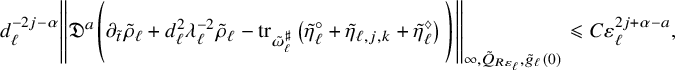 $$ \begin{align}\begin{aligned} d_{\ell}^{-2j-{\alpha}}\Bigg\|\mathfrak{D}^a\Bigg(&\partial_{\tilde t} \tilde{\rho}_{\ell}+d_{\ell}^2\lambda_{\ell}^{-2}\tilde{\rho}_{\ell}-\operatorname{tr}_{\tilde \omega_{\ell}^\sharp}\left(\tilde{\eta}_{\ell}^\circ+\tilde{\eta}_{\ell,j,k}+\tilde{\eta}_{\ell}^\diamondsuit\right)\Bigg)\Bigg\|_{\infty,\tilde Q_{R\varepsilon_{\ell}}, \tilde g_{\ell}(0)}\leqslant C\varepsilon_{\ell}^{2j+{\alpha}-a}, \end{aligned} \end{align} $$
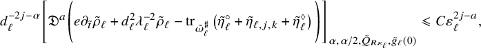 $$ \begin{align}\begin{aligned} d_{\ell}^{-2j-{\alpha}}\Bigg[\mathfrak{D}^a\Bigg(&e\partial_{\tilde t} \tilde{\rho}_{\ell}+d_{\ell}^2\lambda_{\ell}^{-2}\tilde{\rho}_{\ell}-\operatorname{tr}_{\tilde \omega_{\ell}^\sharp}\left(\tilde{\eta}_{\ell}^\circ+\tilde{\eta}_{\ell,j,k}+\tilde{\eta}_{\ell}^\diamondsuit\right)\Bigg)\Bigg]_{{\alpha},{\alpha}/2,\tilde Q_{R\varepsilon_{\ell}}, \tilde g_{\ell}(0)}\leqslant C\varepsilon_{\ell}^{2j-a}, \end{aligned} \end{align} $$
for fixed
 $R>0$
and
$R>0$
and
 $0\leqslant a\leqslant 2j$
, which is a direct consequence of (4.145), (4.153), (4.181), (4.191) together with (4.209) and (4.229).
$0\leqslant a\leqslant 2j$
, which is a direct consequence of (4.145), (4.153), (4.181), (4.191) together with (4.209) and (4.229).
The goal is then to kill the RHS of (4.110) when
 $j=0$
, and to kill the contributions of
$j=0$
, and to kill the contributions of
 $d_{\ell }^{-2j-{\alpha }}\underline{\tilde {\chi }_{\ell }^{*}}$
,
$d_{\ell }^{-2j-{\alpha }}\underline{\tilde {\chi }_{\ell }^{*}}$
,
 $d_{\ell }^{-2j-{\alpha }}\tilde {\psi }_{\ell ,j,k}$
and
$d_{\ell }^{-2j-{\alpha }}\tilde {\psi }_{\ell ,j,k}$
and
 $d_{\ell }^{-2j-{\alpha }}\tilde A_{\ell ,i,p,k}^{*}$
to (4.132) when
$d_{\ell }^{-2j-{\alpha }}\tilde A_{\ell ,i,p,k}^{*}$
to (4.132) when
 $j\geqslant 1$
. We will split the discussion into three cases (without loss of generality): Subcase A:
$j\geqslant 1$
. We will split the discussion into three cases (without loss of generality): Subcase A:
 $\varepsilon _{\ell }\to +\infty $
, Subcase B:
$\varepsilon _{\ell }\to +\infty $
, Subcase B:
 $\varepsilon _{\ell }\to \varepsilon _\infty>0$
, Subcase C:
$\varepsilon _{\ell }\to \varepsilon _\infty>0$
, Subcase C:
 $\varepsilon _{\ell }\to 0$
as
$\varepsilon _{\ell }\to 0$
as
 $\ell \to +\infty $
where
$\ell \to +\infty $
where
 $\varepsilon _{\ell }=d_{\ell }^{-1}\delta _{\ell }=d_{\ell }^{-1}\lambda _{\ell } e^{-t_{\ell }/2}$
.
$\varepsilon _{\ell }=d_{\ell }^{-1}\delta _{\ell }=d_{\ell }^{-1}\lambda _{\ell } e^{-t_{\ell }/2}$
.
4.12 Subcase A:
$\varepsilon _{\ell }\to +\infty $

In this subcase, the background geometry is diverging in the fiber directions, and similarly to the analogous case in [Reference Hein and Tosatti21, §4.10], we will kill all contributions to (4.132) using parabolic Schauder estimates for the linear heat equation. The Selection Theorem 3.1 will also be used crucially. The argument is quite long and involved because of the complexity of the quantitative estimates satisfied by all the pieces in the decomposition of the solution
 $\tilde {\omega }^{\bullet }_{\ell }$
. We start with the direct analog of the non-cancellation result in [Reference Hein and Tosatti21, Proposition 4.7].
$\tilde {\omega }^{\bullet }_{\ell }$
. We start with the direct analog of the non-cancellation result in [Reference Hein and Tosatti21, Proposition 4.7].
Proposition 4.8. The following inequalities hold for all
 $0\leqslant {\alpha }<1$
,
$0\leqslant {\alpha }<1$
,
 $a\in \mathbb {N}$
,
$a\in \mathbb {N}$
,
 $1\leqslant i\leqslant j$
,
$1\leqslant i\leqslant j$
,
 $1\leqslant p\leqslant N_{i,k}$
and all
$1\leqslant p\leqslant N_{i,k}$
and all
 $R>0$
:
$R>0$
:
 $$ \begin{align} [\mathfrak{D}^a {i\partial\bar\partial}\underline{\hat{\varphi }_{\ell}}]_{{\alpha},{\alpha}/2,\hat Q_R }\leqslant C[\mathfrak{D}^{a}_{\textbf{bt}}{i\partial\bar\partial} \hat\varphi_{\ell}]_{{\alpha},{\alpha}/2,\textrm{base},\hat Q_R,g_X}+C\left(\frac{R}{\lambda_{\ell}} \right)^{1-{\alpha}}\sum_{b=0}^{a} \lambda_{\ell}^{-{\alpha}} \|\mathfrak{D}^b{i\partial\bar\partial} \hat\varphi_{\ell}\|_{\infty,\hat Q_R,g_X}, \end{align} $$
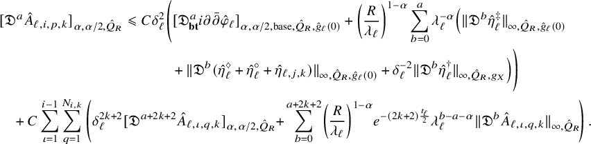 $$ \begin{align} &[\mathfrak{D}^{a} \hat A_{\ell,i,p,k}]_{{\alpha},{\alpha}/2,\hat Q_R }\leqslant C\delta_{\ell}^2 \Bigg( [\mathfrak{D}^{a}_{\textbf{bt}}{i\partial\bar\partial} \hat\varphi_{\ell}]_{{\alpha},{\alpha}/2,\textrm{base},\hat Q_R,\hat g_{\ell}(0)}+\left(\frac{R}{\lambda_{\ell}} \right)^{1-{\alpha}}\sum_{b=0}^{a} \lambda_{\ell}^{-{\alpha}}\Big( \|\mathfrak{D}^b \hat \eta_{\ell}^\ddagger\|_{\infty,\hat Q_R,\hat g_{\ell}(0)}\nonumber\\&\qquad\qquad\qquad\qquad\qquad\qquad +\|\mathfrak{D}^b(\hat\eta_{\ell}^\diamondsuit+\hat\eta_{\ell}^\circ+\hat \eta_{\ell,j,k}) \|_{\infty,\hat Q_R,\hat g_{\ell}(0)} +\delta_{\ell}^{-2}\|\mathfrak{D}^b\hat \eta_{\ell}^\dagger\|_{\infty,\hat Q_R,g_X}\Big)\Bigg)\nonumber\\& \quad +C\sum_{\iota=1}^{i-1}\sum_{q=1}^{N_{i,k}}\left(\delta_{\ell}^{2k+2} [\mathfrak{D}^{a+2k+2}\hat A_{\ell,\iota,q,k}]_{{\alpha},{\alpha}/2,\hat Q_R}{\kern-2pt}+{\kern-3pt}\sum_{b=0}^{a+2k+2} {\kern-3pt}\left(\frac{R}{\lambda_{\ell}}\right)^{1-{\alpha}}{\kern-2pt} e^{-(2k+2)\frac{t_{\ell}}{2}}\lambda_{\ell}^{b-a-{\alpha}}\|\mathfrak{D}^b \hat A_{\ell,\iota,q,k}\|_{\infty,\hat Q_R}\!\right). \end{align} $$
Proof. The proof is very similar to that of [Reference Hein and Tosatti21, Proposition 4.7], so we only highlight the differences. The starting point of the proof (Claim 1 in [Reference Hein and Tosatti21, Proof of Proposition 4.7]) is to express
 ${i\partial \bar \partial }\underline{\hat {\varphi }_{\ell }}$
and
${i\partial \bar \partial }\underline{\hat {\varphi }_{\ell }}$
and
 $\hat A_{\ell ,i,p,k}$
as pushforwards of quantities on the total space. This step is essentially identical here, with the only difference being that in the formula for
$\hat A_{\ell ,i,p,k}$
as pushforwards of quantities on the total space. This step is essentially identical here, with the only difference being that in the formula for
 $\hat A_{\ell ,i,p,k}$
, the term
$\hat A_{\ell ,i,p,k}$
, the term
 $e^{-(2k+2)\frac {t}{2}}$
in [Reference Hein and Tosatti21, (4.204)] now becomes
$e^{-(2k+2)\frac {t}{2}}$
in [Reference Hein and Tosatti21, (4.204)] now becomes
 $e^{-(2k+2)(t_{\ell }+\lambda _{\ell }^{-2}\hat t)/2}.$
The extra time-dependent constant
$e^{-(2k+2)(t_{\ell }+\lambda _{\ell }^{-2}\hat t)/2}.$
The extra time-dependent constant
 $e^{-(2k+2)\lambda _{\ell }^{-2}\frac {\hat t}{2}}$
will then also need to be differentiated in the analog of [Reference Hein and Tosatti21, (4.234)], which gives us extra cross terms in the analog of [Reference Hein and Tosatti21, (4.247)], but which can be estimated in a similar way resulting in the same upper bound as stated.
$e^{-(2k+2)\lambda _{\ell }^{-2}\frac {\hat t}{2}}$
will then also need to be differentiated in the analog of [Reference Hein and Tosatti21, (4.234)], which gives us extra cross terms in the analog of [Reference Hein and Tosatti21, (4.247)], but which can be estimated in a similar way resulting in the same upper bound as stated.
The next step is to try to commute the derivative
 $\mathfrak {D}^a$
with the pushforward, and make the commutation error terms explicit. Recalling that
$\mathfrak {D}^a$
with the pushforward, and make the commutation error terms explicit. Recalling that
 $\mathfrak {D}^{a}$
is a sum of terms of the form
$\mathfrak {D}^{a}$
is a sum of terms of the form
 ${\mathbb {D}}^p\partial _{\hat {t}}^q$
, we observe that
${\mathbb {D}}^p\partial _{\hat {t}}^q$
, we observe that
 $\partial _{\hat {t}}^q$
trivially commutes with pushforwards (with no error terms), while the commutation of
$\partial _{\hat {t}}^q$
trivially commutes with pushforwards (with no error terms), while the commutation of
 ${\mathbb {D}}^p$
gives exactly the same result as in Claim 2 [Reference Hein and Tosatti21, Proof of Proposition 4.7]; cf. [Reference Hein and Tosatti21, (4.223), (4.240)].
${\mathbb {D}}^p$
gives exactly the same result as in Claim 2 [Reference Hein and Tosatti21, Proof of Proposition 4.7]; cf. [Reference Hein and Tosatti21, (4.223), (4.240)].
The last step is to estimate the Hölder difference quotient of
 $\mathfrak {D}^a{i\partial \bar \partial }\underline{\hat {\varphi }_{\ell }}$
and
$\mathfrak {D}^a{i\partial \bar \partial }\underline{\hat {\varphi }_{\ell }}$
and
 $\mathfrak {D}^a\hat A_{\ell ,i,p,k}$
. This is now a space-time Hölder difference quotient, which we can split with the triangle inequality into a space-only difference quotient (which is estimated following the method of Claim 3 in [Reference Hein and Tosatti21, Proof of Proposition 4.7] verbatim), and a time-only difference quotient, which again commutes with pushforward and so can be estimated trivially without any further error terms. This completes the outline of the proof.
$\mathfrak {D}^a\hat A_{\ell ,i,p,k}$
. This is now a space-time Hölder difference quotient, which we can split with the triangle inequality into a space-only difference quotient (which is estimated following the method of Claim 3 in [Reference Hein and Tosatti21, Proof of Proposition 4.7] verbatim), and a time-only difference quotient, which again commutes with pushforward and so can be estimated trivially without any further error terms. This completes the outline of the proof.
For notation convenience, we will denote
 $\hat \eta _{\ell }={i\partial \bar \partial }\hat \varphi _{\ell }=\hat \eta _{\ell }^\dagger +\hat \eta _{\ell }^\ddagger +\hat \eta _{\ell }^\diamondsuit +\hat \eta _{\ell }^\circ +\hat \eta _{\ell ,j,k}$
.
$\hat \eta _{\ell }={i\partial \bar \partial }\hat \varphi _{\ell }=\hat \eta _{\ell }^\dagger +\hat \eta _{\ell }^\ddagger +\hat \eta _{\ell }^\diamondsuit +\hat \eta _{\ell }^\circ +\hat \eta _{\ell ,j,k}$
.
4.12.1 The case
$j=0$

Unlike [Reference Hein and Tosatti21], the case
 $j=0$
requires a separate treatment. This is due to the fact that the Monge-Ampère equation (4.216) is naturally a parabolic PDE for the scalar potential
$j=0$
requires a separate treatment. This is due to the fact that the Monge-Ampère equation (4.216) is naturally a parabolic PDE for the scalar potential
 $\tilde {\rho }_{\ell }$
, which, however, does not have a uniform bound on its
$\tilde {\rho }_{\ell }$
, which, however, does not have a uniform bound on its
 $L^\infty $
norm, which is an issue when applying Schauder estimates. This is remedied in two different ways according to whether
$L^\infty $
norm, which is an issue when applying Schauder estimates. This is remedied in two different ways according to whether
 $j=0$
or
$j=0$
or
 $j>0$
. In this subsection, we treat the case
$j>0$
. In this subsection, we treat the case
 $j=0$
.
$j=0$
.
The first crucial claim is that for any fixed
 $R>0$
, we have
$R>0$
, we have
 $$ \begin{align} d_{\ell}^{-\alpha}[(\mathcal{E}_1+\mathcal{E}_2+\mathcal{E}_3)]_{{\alpha},{\alpha}/2,\tilde{Q}_{R},\tilde{g}_{\ell}(0)}=o(1). \end{align} $$
For the term
 $\mathcal {E}_1$
, we have already proved an even strong result in (4.221), so we consider
$\mathcal {E}_1$
, we have already proved an even strong result in (4.221), so we consider
 $\mathcal {E}_2+\mathcal {E}_3$
, which when
$\mathcal {E}_2+\mathcal {E}_3$
, which when
 $j=0$
equals
$j=0$
equals
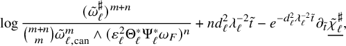 $$ \begin{align} \log \frac{(\tilde{\omega}_{\ell}^\sharp)^{m+n}}{ \binom{m+n}{m}\tilde \omega_{\ell,\mathrm{can}} ^m \wedge (\varepsilon_{\ell}^2 \Theta_{\ell}^{*}\Psi_{\ell}^{*} \omega_F)^n}+nd_{\ell}^2\lambda_{\ell}^{-2}\tilde t -e^{-d_{\ell}^2\lambda_{\ell}^{-2}\tilde{t}}\partial_{\tilde{t}}\underline{\tilde{\chi}^\sharp_{\ell}}, \end{align} $$
and since
 $\partial _{\tilde {t}}\underline{\tilde {\chi }^\sharp _{\ell }}$
is a constant (in space and time), it is clear that
$\partial _{\tilde {t}}\underline{\tilde {\chi }^\sharp _{\ell }}$
is a constant (in space and time), it is clear that
 $$ \begin{align} d_{\ell}^{-\alpha}[nd_{\ell}^2\lambda_{\ell}^{-2}\tilde t -e^{-d_{\ell}^2\lambda_{\ell}^{-2}\tilde{t}}\partial_{\tilde{t}}\underline{\tilde{\chi}^\sharp_{\ell}}]_{{\alpha},{\alpha}/2,\tilde{Q}_{R},\tilde{g}_{\ell}(0)}=o(1), \end{align} $$
and we are left with showing that
 $$ \begin{align} d_{\ell}^{-\alpha}\left[\log \frac{(\tilde{\omega}_{\ell}^\sharp)^{m+n}}{ \binom{m+n}{m}\tilde \omega_{\ell,\mathrm{can}} ^m \wedge (\varepsilon_{\ell}^2 \Theta_{\ell}^{*}\Psi_{\ell}^{*} \omega_F)^n}\right]_{{\alpha},{\alpha}/2,\tilde{Q}_{R},\tilde{g}_{\ell}(0)}=o(1). \end{align} $$
For this, we pass to the check picture using the diffeomorphisms
 $\Pi _{\ell }$
in (4.285) below, scaling geometric quantities by
$\Pi _{\ell }$
in (4.285) below, scaling geometric quantities by
 $\varepsilon _{\ell }^{-2}$
, so that the quantity in (4.237) equals
$\varepsilon _{\ell }^{-2}$
, so that the quantity in (4.237) equals
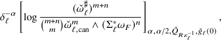 $$ \begin{align} \delta_{\ell}^{-\alpha}\left[\log \frac{(\check\omega_{\ell}^\sharp)^{m+n}}{ \binom{m+n}{m}\check \omega_{\ell,\mathrm{can}} ^m \wedge (\Sigma_{\ell}^{*} \omega_F)^n}\right]_{{\alpha},{\alpha}/2,\check{Q}_{R\varepsilon_{\ell}^{-1}},\check{g}_{\ell}(0)}, \end{align} $$
and using (3.23), together with the facts that
 $[\check {\eta }^\ddagger _{\ell }]_{{\alpha },{\alpha }/2,\check {Q}_{R\varepsilon _{\ell }^{-1}},\check {g}_{\ell }(0)}=0,$
and
$[\check {\eta }^\ddagger _{\ell }]_{{\alpha },{\alpha }/2,\check {Q}_{R\varepsilon _{\ell }^{-1}},\check {g}_{\ell }(0)}=0,$
and
 $\delta _{\ell }^{-\alpha }[\check {\omega }_{\ell ,\mathrm {can}}]_{{\alpha },{\alpha }/2,\check {Q}_{R\varepsilon _{\ell }^{-1}},\check {g}_{\ell }(0)}\leqslant C\lambda _{\ell }^{-\alpha }=o(1),$
we see that (4.237) holds.
$\delta _{\ell }^{-\alpha }[\check {\omega }_{\ell ,\mathrm {can}}]_{{\alpha },{\alpha }/2,\check {Q}_{R\varepsilon _{\ell }^{-1}},\check {g}_{\ell }(0)}\leqslant C\lambda _{\ell }^{-\alpha }=o(1),$
we see that (4.237) holds.
The next issue we face is that (4.144) does not provide us with uniform bounds on
 $d_{\ell }^{-{\alpha }}\|\mathfrak {D}^{2}\tilde {\psi }_{\ell ,0,k}\|_{\infty ,\tilde {Q}_R,\tilde {g}_{\ell }(0)},$
for any fixed R, so we are unable to pass
$d_{\ell }^{-{\alpha }}\|\mathfrak {D}^{2}\tilde {\psi }_{\ell ,0,k}\|_{\infty ,\tilde {Q}_R,\tilde {g}_{\ell }(0)},$
for any fixed R, so we are unable to pass
 $d_{\ell }^{-{\alpha }}\partial _{\tilde {t}}\tilde {\psi }_{\ell ,0,k}$
or
$d_{\ell }^{-{\alpha }}\partial _{\tilde {t}}\tilde {\psi }_{\ell ,0,k}$
or
 $d_{\ell }^{-{\alpha }}{i\partial \bar \partial }\tilde {\psi }_{\ell ,0,k}$
to a limit. To fix this, we use the method of [Reference Hein and Tosatti20, Subclaim 1.3], by replacing the whole fiber Y with a coordinate chart and performing a jet subtraction to
$d_{\ell }^{-{\alpha }}{i\partial \bar \partial }\tilde {\psi }_{\ell ,0,k}$
to a limit. To fix this, we use the method of [Reference Hein and Tosatti20, Subclaim 1.3], by replacing the whole fiber Y with a coordinate chart and performing a jet subtraction to
 $d_{\ell }^{-{\alpha }}\tilde {\psi }_{\ell ,0,k}$
so that the remainder is locally
$d_{\ell }^{-{\alpha }}\tilde {\psi }_{\ell ,0,k}$
so that the remainder is locally
 $C^2$
convergent.
$C^2$
convergent.
To fix this, recall that
 $\tilde {g}_{\ell }(\tilde {t}) = g_{\mathbb {C}^m} + \varepsilon _{\ell }^2 e^{-d_{\ell }^2\lambda _{\ell }^{-2}\tilde {t}} g_{Y,0}$
. Let
$\tilde {g}_{\ell }(\tilde {t}) = g_{\mathbb {C}^m} + \varepsilon _{\ell }^2 e^{-d_{\ell }^2\lambda _{\ell }^{-2}\tilde {t}} g_{Y,0}$
. Let
 $\mathbf {x}^{2m+1}, \ldots , \mathbf {x}^{2m+2n}$
be normal coordinates for
$\mathbf {x}^{2m+1}, \ldots , \mathbf {x}^{2m+2n}$
be normal coordinates for
 $g_{Y,0}$
centered at
$g_{Y,0}$
centered at
 $y_{\ell }$
. Viewed as a map from Y to
$y_{\ell }$
. Viewed as a map from Y to
 $\mathbb {R}^{2n}$
, these depend on
$\mathbb {R}^{2n}$
, these depend on
 $\ell $
, but we prefer to instead pull back our setup to
$\ell $
, but we prefer to instead pull back our setup to
 $\mathbb {R}^{2n}$
under the inverse map. In this sense, we may then assume without loss that
$\mathbb {R}^{2n}$
under the inverse map. In this sense, we may then assume without loss that
 $$ \begin{align} \left|\frac{\partial^\iota}{\partial\mathbf{x}^\iota}(g_{Y,0}(\mathbf{x})_{ab}-\delta_{ab})\right| \leqslant \frac{1}{100}|\mathbf{x}|^{2-\iota}\,\;\mathrm{for}\;\, |\mathbf{x}| \leqslant 2\;\,\mathrm{ and}\;\,\iota=0,1. \end{align} $$
This is possible thanks to the compactness of Y. Define
 $\tilde {\mathbf {x}}^j = \varepsilon _{\ell } \mathbf {x}^j$
, so that
$\tilde {\mathbf {x}}^j = \varepsilon _{\ell } \mathbf {x}^j$
, so that
 $\tilde {\mathbf {x}}^{2m+1}, \ldots , \tilde {\mathbf {x}}^{2m+2n}$
are normal coordinates for
$\tilde {\mathbf {x}}^{2m+1}, \ldots , \tilde {\mathbf {x}}^{2m+2n}$
are normal coordinates for
 $\varepsilon _{\ell }^2 g_{Y,0}$
centered at
$\varepsilon _{\ell }^2 g_{Y,0}$
centered at
 $y_{\ell }$
. Formally also write
$y_{\ell }$
. Formally also write
 $\tilde {\mathbf {x}}^1, \ldots , \tilde {\mathbf {x}}^{2m}$
for the standard real coordinates on
$\tilde {\mathbf {x}}^1, \ldots , \tilde {\mathbf {x}}^{2m}$
for the standard real coordinates on
 $\mathbb {C}^m$
. Then
$\mathbb {C}^m$
. Then
 $\tilde {\mathbf {x}}^1, \ldots , \tilde {\mathbf {x}}^{2m+2n}$
are normal coordinates for
$\tilde {\mathbf {x}}^1, \ldots , \tilde {\mathbf {x}}^{2m+2n}$
are normal coordinates for
 $\tilde {g}_{\ell }(0)$
centered at
$\tilde {g}_{\ell }(0)$
centered at
 $\tilde {x}_{\ell }$
with
$\tilde {x}_{\ell }$
with
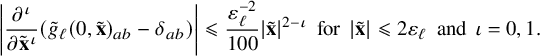 $$ \begin{align} \left|\frac{\partial^\iota}{\partial\tilde{\mathbf{x}}^\iota}(\tilde{g}_{\ell}(0, \tilde{\mathbf{x}})_{ab}-\delta_{ab})\right| \leqslant \frac{\varepsilon_{\ell}^{-2}}{100}|\tilde{\mathbf{x}}|^{2-\iota}\,\;\mathrm{for}\;\, |\tilde{\mathbf{x}}| \leqslant 2\varepsilon_{\ell}\;\,\mathrm{and}\;\,\iota=0,1. \end{align} $$
We then define a function
 $\tilde {\psi }^\sharp _{\ell ,0,k}$
on
$\tilde {\psi }^\sharp _{\ell ,0,k}$
on
 $\tilde {Q}_{2\varepsilon _{\ell }}$
to be the parabolic
$\tilde {Q}_{2\varepsilon _{\ell }}$
to be the parabolic
 $2$
nd order Taylor polynomial of
$2$
nd order Taylor polynomial of
 $\tilde {\psi }_{\ell ,0,k}$
at the space-time origin
$\tilde {\psi }_{\ell ,0,k}$
at the space-time origin
 $(0,0)$
, using the spatial coordinates
$(0,0)$
, using the spatial coordinates
 $\tilde {\mathbf {x}}^i,1\leqslant i\leqslant 2m+2n$
, and we define also
$\tilde {\mathbf {x}}^i,1\leqslant i\leqslant 2m+2n$
, and we define also
 $\tilde {\psi }^{*}_{\ell ,0,k}:=\tilde {\psi }_{\ell ,0,k}-\tilde {\psi }^\sharp _{\ell ,0,k}.$
Since all Euclidean derivatives of
 $\tilde {\psi }^{*}_{\ell ,0,k}$
of order at most
$\tilde {\psi }^{*}_{\ell ,0,k}$
of order at most
 $2$
vanish at
$2$
vanish at
 $(0,0)$
, using the formula in [Reference Hein and Tosatti21, Lemma 2.3] relating
$(0,0)$
, using the formula in [Reference Hein and Tosatti21, Lemma 2.3] relating
 ${\mathbb {D}}$
-derivatives and ordinary derivatives, we see that
${\mathbb {D}}$
-derivatives and ordinary derivatives, we see that
 $\mathfrak {D}^\iota \tilde {\psi }^{*}_{\ell ,0,k}\big |_{(0,0)}=0,0\leqslant \iota \leqslant 2$
.
$\mathfrak {D}^\iota \tilde {\psi }^{*}_{\ell ,0,k}\big |_{(0,0)}=0,0\leqslant \iota \leqslant 2$
.
Next, we prove the following bounds for
 $d_{\ell }^{-\alpha }\tilde {\psi }^\sharp _{\ell ,0,k}$
: for all
$d_{\ell }^{-\alpha }\tilde {\psi }^\sharp _{\ell ,0,k}$
: for all
 $\iota \geqslant 0, 0<\beta <1$
, and
$\iota \geqslant 0, 0<\beta <1$
, and
 $0<R\leqslant \varepsilon _{\ell }$
,
$0<R\leqslant \varepsilon _{\ell }$
,
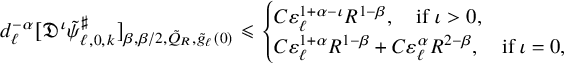 $$ \begin{align} d_{\ell}^{-\alpha}[\mathfrak{D}^\iota\tilde{\psi}^\sharp_{\ell,0,k}]_{{\beta},{\beta}/2,\tilde{Q}_{R},\tilde{g}_{\ell}(0)}\leqslant \begin{cases} C\varepsilon_{\ell}^{1+\alpha-\iota}R^{1-\beta},\quad \text{if }\iota>0,\\ C\varepsilon_{\ell}^{1+\alpha}R^{1-\beta}+C\varepsilon_{\ell}^{\alpha}R^{2-\beta},\quad \text{if }\iota=0, \end{cases} \end{align} $$
 $$ \begin{align} d_{\ell}^{-\alpha}\|\mathfrak{D}^\iota\tilde{\psi}^\sharp_{\ell,0,k}\|_{\infty,\tilde{Q}_{R},\tilde{g}_{\ell}(0)}\leqslant C\varepsilon_{\ell}^{2+\alpha-\iota}. \end{align} $$
To prove this claim, note that for any
 $z\in B_1,$
the metric
$z\in B_1,$
the metric
 $g_{Y,z}$
is at bounded distance to
$g_{Y,z}$
is at bounded distance to
 $g_{Y,0}$
in
$g_{Y,0}$
in
 $C^\infty (Y)$
, and thus,
$C^\infty (Y)$
, and thus,
 $$ \begin{align} |\nabla^{\iota,\tilde{g}_{\ell}(0)}\tilde{g}_{\tilde{z}}(\tilde{t})|_{\tilde{g}_{\ell}(0)} \leqslant C_\iota\varepsilon_{\ell}^{-\iota} \;\,\mathrm{on}\;\,\tilde{Q}_R, \end{align} $$
for all
 $\iota \geqslant 1, R\leqslant \varepsilon _{\ell }$
.
$\iota \geqslant 1, R\leqslant \varepsilon _{\ell }$
.
Let us also note the following bounds for the Euclidean derivatives
 $\tilde {\psi }_{\ell ,0,k}$
,
$\tilde {\psi }_{\ell ,0,k}$
,
 $$ \begin{align} d_{\ell}^{-\alpha}|\partial^{|\gamma|}\partial_{\tilde{t}}^q\tilde{\psi}_{\ell,0,k}|(\tilde{\mathbf{x}}_{\ell},\tilde{t}_{\ell})\leqslant C\varepsilon_{\ell}^{2+\alpha-|\gamma|-2q}, \end{align} $$
for all multiindices
 $\gamma $
with
$\gamma $
with
 $|\gamma |+2q\leqslant 2$
. To see this, we first apply the diffeomorphism
$|\gamma |+2q\leqslant 2$
. To see this, we first apply the diffeomorphism
 $$ \begin{align*}\Lambda_{\ell}:\check{Q}_2\to \tilde{Q}_{2\varepsilon_{\ell}},\quad (\tilde{\mathbf{x}}^1,\dots,\tilde{\mathbf{x}}^{2m+2n},\tilde{t})=\Lambda_{\ell}(\check{\mathbf{x}}^1,\dots,\check{\mathbf{x}}^{2m+2n},\check{t}) =(\varepsilon_{\ell}\check{\mathbf{x}}^1,\dots,\varepsilon_{\ell}\check{\mathbf{x}}^{2m+2n},\varepsilon_{\ell}^2\check{t}),\end{align*} $$
and pull back metrics and
 $2$
-forms, as well as
$2$
-forms, as well as
 $\tilde {\psi }_{\ell ,0,k}$
, via
$\tilde {\psi }_{\ell ,0,k}$
, via
 $\Lambda _{\ell }$
, multiply them by
$\Lambda _{\ell }$
, multiply them by
 $\varepsilon _{\ell }^{-2}$
and denote the resulting objects with a check, so, for example, the metrics
$\varepsilon _{\ell }^{-2}$
and denote the resulting objects with a check, so, for example, the metrics
 $\check {g}_{\ell }(0)=\varepsilon _{\ell }^{-2}\Lambda _{\ell }^{*}\tilde {g}_{\ell }(0)$
on
$\check {g}_{\ell }(0)=\varepsilon _{\ell }^{-2}\Lambda _{\ell }^{*}\tilde {g}_{\ell }(0)$
on
 $\check {Q}_2$
are smoothly convergent to a fixed metric (smoothly comparable to Euclidean), and the pulled back complex structure is approaching the Euclidean one (without loss). The bounds (4.144) transform to
$\check {Q}_2$
are smoothly convergent to a fixed metric (smoothly comparable to Euclidean), and the pulled back complex structure is approaching the Euclidean one (without loss). The bounds (4.144) transform to
 $$\begin{align*}d_{\ell}^{-\alpha}\|\mathfrak{D}^\iota\check{\psi}_{\ell,0,k}\|_{\infty,\check{Q}_{2},\check{g}_{\ell}(0)}\leqslant C\varepsilon_{\ell}^{2+\alpha},\quad d_{\ell}^{-\alpha}[\mathfrak{D}^\iota\check{\psi}_{\ell,0,k}]_{{\alpha},{\alpha}/2,\check{Q}_{2},\check{g}_{\ell}(0)}\leqslant C\varepsilon_{\ell}^{2+\alpha}, \end{align*}$$
for
 $0\leqslant \iota \leqslant 2$
. Since
$0\leqslant \iota \leqslant 2$
. Since
 $\check {g}_{\ell }(0)$
is approximately Euclidean, [Reference Hein and Tosatti21, Lemma 2.6] gives us that the Euclidean
$\check {g}_{\ell }(0)$
is approximately Euclidean, [Reference Hein and Tosatti21, Lemma 2.6] gives us that the Euclidean
 $C^{\alpha ,{\alpha }/2}$
norm of
$C^{\alpha ,{\alpha }/2}$
norm of
 $d_{\ell }^{-\alpha }\check {\psi }_{\ell ,0,k}$
is also bounded by
$d_{\ell }^{-\alpha }\check {\psi }_{\ell ,0,k}$
is also bounded by
 $C\varepsilon _{\ell }^{2+\alpha }$
, and translating these back to the tilde picture proves (4.244).
$C\varepsilon _{\ell }^{2+\alpha }$
, and translating these back to the tilde picture proves (4.244).
First, we prove (4.241). Given
 $(\tilde {x},\tilde {t}),(\tilde {x}',\tilde {t}')\in \tilde {Q}_R$
, call
$(\tilde {x},\tilde {t}),(\tilde {x}',\tilde {t}')\in \tilde {Q}_R$
, call
 $d=d^{\tilde {g}_{\ell }(0)}(\tilde {x},\tilde {x}')+|\tilde {t}-\tilde {t}'|^{\frac {1}{2}},$
and given
$d=d^{\tilde {g}_{\ell }(0)}(\tilde {x},\tilde {x}')+|\tilde {t}-\tilde {t}'|^{\frac {1}{2}},$
and given
 $p,q\geqslant 0$
with
$p,q\geqslant 0$
with
 $p+2q=\iota $
, we can bound
$p+2q=\iota $
, we can bound
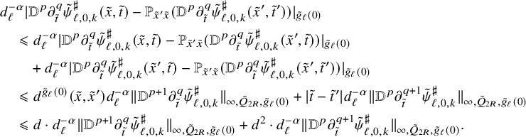 $$ \begin{align}\begin{aligned} &d_{\ell}^{-\alpha}|{\mathbb{D}}^p\partial_{\tilde{t}}^q\tilde{\psi}^\sharp_{\ell,0,k}(\tilde{x},\tilde{t})-\mathbb{P}_{\tilde{x}'\tilde{x}}({\mathbb{D}}^p\partial_{\tilde{t}}^q\tilde{\psi}^\sharp_{\ell,0,k}(\tilde{x}',\tilde{t}'))|_{\tilde{g}_{\ell}(0)}\\&\quad\leqslant d_{\ell}^{-\alpha}|{\mathbb{D}}^p\partial_{\tilde{t}}^q\tilde{\psi}^\sharp_{\ell,0,k}(\tilde{x},\tilde{t})-\mathbb{P}_{\tilde{x}'\tilde{x}}({\mathbb{D}}^p\partial_{\tilde{t}}^q\tilde{\psi}^\sharp_{\ell,0,k}(\tilde{x}',\tilde{t}))|_{\tilde{g}_{\ell}(0)}\\&\qquad+d_{\ell}^{-\alpha}|{\mathbb{D}}^p\partial_{\tilde{t}}^q\tilde{\psi}^\sharp_{\ell,0,k}(\tilde{x}',\tilde{t})-\mathbb{P}_{\tilde{x}'\tilde{x}}({\mathbb{D}}^p\partial_{\tilde{t}}^q\tilde{\psi}^\sharp_{\ell,0,k}(\tilde{x}',\tilde{t}'))|_{\tilde{g}_{\ell}(0)}\\&\quad\leqslant d^{\tilde{g}_{\ell}(0)}(\tilde{x},\tilde{x}')d_{\ell}^{-\alpha}\|{\mathbb{D}}^{p+1}\partial_{\tilde{t}}^q\tilde{\psi}^\sharp_{\ell,0,k}\|_{\infty,\tilde{Q}_{2R},\tilde{g}_{\ell}(0)} +|\tilde{t}-\tilde{t}'|d_{\ell}^{-\alpha}\|{\mathbb{D}}^{p}\partial_{\tilde{t}}^{q+1}\tilde{\psi}^\sharp_{\ell,0,k}\|_{\infty,\tilde{Q}_{2R},\tilde{g}_{\ell}(0)}\\&\quad\leqslant d\cdot d_{\ell}^{-\alpha}\|{\mathbb{D}}^{p+1}\partial_{\tilde{t}}^q\tilde{\psi}^\sharp_{\ell,0,k}\|_{\infty,\tilde{Q}_{2R},\tilde{g}_{\ell}(0)} +d^2\cdot d_{\ell}^{-\alpha}\|{\mathbb{D}}^{p}\partial_{\tilde{t}}^{q+1}\tilde{\psi}^\sharp_{\ell,0,k}\|_{\infty,\tilde{Q}_{2R},\tilde{g}_{\ell}(0)}. \end{aligned} \end{align} $$
Since
 $\tilde {\psi }^\sharp _{\ell ,0,k}$
is the sum of a polynomial of degree at most
$\tilde {\psi }^\sharp _{\ell ,0,k}$
is the sum of a polynomial of degree at most
 $2$
in the
$2$
in the
 $\tilde {\mathbf {x}}$
variables (constant in time), and of a polynomial of degree at most
$\tilde {\mathbf {x}}$
variables (constant in time), and of a polynomial of degree at most
 $1$
in the
$1$
in the
 $\tilde {t}$
variable (constant in space), it follows that
$\tilde {t}$
variable (constant in space), it follows that
 ${\mathbb {D}}^{p+1}\partial _{\tilde {t}}^q\tilde {\psi }^\sharp _{\ell ,0,k}\equiv 0$
unless
${\mathbb {D}}^{p+1}\partial _{\tilde {t}}^q\tilde {\psi }^\sharp _{\ell ,0,k}\equiv 0$
unless
 $q=0$
(hence,
$q=0$
(hence,
 $\iota =p$
), and that
$\iota =p$
), and that
 ${\mathbb {D}}^{p}\partial _{\tilde {t}}^{q+1}\tilde {\psi }^\sharp _{\ell ,0,k}\equiv 0$
unless
${\mathbb {D}}^{p}\partial _{\tilde {t}}^{q+1}\tilde {\psi }^\sharp _{\ell ,0,k}\equiv 0$
unless
 $p=q=0$
(and hence,
$p=q=0$
(and hence,
 $\iota =0$
).
$\iota =0$
).
We consider these two cases separately, so we first bound the term with
 ${\mathbb {D}}^{\iota +1}\tilde {\psi }^\sharp _{\ell ,0,k}$
(which is equal to
${\mathbb {D}}^{\iota +1}\tilde {\psi }^\sharp _{\ell ,0,k}$
(which is equal to
 ${\mathbb {D}}^{\iota +1}$
applied to the spatial Taylor polynomial only), by converting
${\mathbb {D}}^{\iota +1}$
applied to the spatial Taylor polynomial only), by converting
 ${\mathbb {D}}^{\iota +1}$
into
${\mathbb {D}}^{\iota +1}$
into
 $\nabla ^{\iota +1}$
using [Reference Hein and Tosatti21, Lemma 2.3] (which involves a certain tensor
$\nabla ^{\iota +1}$
using [Reference Hein and Tosatti21, Lemma 2.3] (which involves a certain tensor
 $\mathbf {A}$
), and estimating
$\mathbf {A}$
), and estimating
 $$ \begin{align} d_{\ell}^{-\alpha}\|{\mathbb{D}}^{\iota+1} \tilde{\psi}^\sharp_{\ell,0,k}\|_{\infty,\tilde{Q}_{2R},\tilde{g}_{\ell}(0)} \end{align} $$
 $$ \begin{align} \leqslant \bigg\|d_{\ell}^{-\alpha}&\left(\left( \frac{\partial}{\partial\tilde{\mathbf{x}}} + \Gamma^{\tilde{g}_{\tilde{z}}(\tilde{t})}(\tilde{\mathbf{x}})\right)^{\iota+1}+ \sum_{r=0}^{\iota-1}\nabla_{z,y,\tilde{z}}^{\iota-1-r}\mathbf{A}\circledast\left( \frac{\partial}{\partial\tilde{\mathbf{x}}} + \Gamma^{\tilde{g}_{\tilde{z}}(\tilde{t})}(\tilde{\mathbf{x}})\right)^{r}\right) \end{align} $$
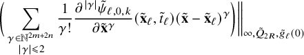 $$ \begin{align} &\bigg(\sum_{\substack{\gamma\in\mathbb{N}^{2m+2n}\\ |\gamma|\leqslant 2}} \frac{1}{\gamma!} \frac{\partial^{|\gamma|}\tilde{\psi}_{\ell,0,k}}{\partial\tilde{\mathbf{x}}^\gamma}(\tilde{\mathbf{x}}_{\ell},\tilde{t}_{\ell})(\tilde{\mathbf{x}} - \tilde{\mathbf{x}}_{\ell})^\gamma \bigg) \bigg\|_{\infty,\tilde{Q}_{2R},\tilde{g}_{\ell}(0)} \end{align} $$
and estimating the big
 $L^\infty $
norm by
$L^\infty $
norm by
 $C\varepsilon _{\ell }^{1+\alpha -\iota }$
, as follows.
$C\varepsilon _{\ell }^{1+\alpha -\iota }$
, as follows.
(1) We have
 $ \partial ^b \Gamma = O( \varepsilon _{\ell }^{-b-1})$
by (4.240) and (4.243).
$ \partial ^b \Gamma = O( \varepsilon _{\ell }^{-b-1})$
by (4.240) and (4.243).
(2) The
 $\mathbf {A}$
-tensor in the tilde picture is bounded by
$\mathbf {A}$
-tensor in the tilde picture is bounded by
 $O(\varepsilon _{\ell }^{-2})$
, since it is schematically of the same type as
$O(\varepsilon _{\ell }^{-2})$
, since it is schematically of the same type as
 $\partial \Gamma $
. By the same reason,
$\partial \Gamma $
. By the same reason,
 $\nabla _{z,y,\tilde {z}}^{r}\mathbf {A}$
is
$\nabla _{z,y,\tilde {z}}^{r}\mathbf {A}$
is
 $O(\varepsilon _{\ell }^{-r-2})$
.
$O(\varepsilon _{\ell }^{-r-2})$
.
(3) Writing
 $d_{\ell }^{-\alpha }\tilde {\psi }_{\ell ,0,k}=\psi $
, we can then estimate
$d_{\ell }^{-\alpha }\tilde {\psi }_{\ell ,0,k}=\psi $
, we can then estimate
 $$ \begin{align}\begin{aligned} (\partial + \Gamma)^r((\partial^{|\gamma|}\psi)(\tilde{\mathbf{x}}_{\ell},\tilde{t}_{\ell}) (\tilde{\mathbf{x}}-\tilde{\mathbf{x}}_{\ell})^\gamma) &=(\partial^{|\gamma|}\psi)(\tilde{\mathbf{x}}_{\ell},\tilde{t}_{\ell}) \sum \partial^{a_1}\Gamma \cdots \partial^{a_{\ell}}\Gamma \cdot \partial^{b} (\tilde{\mathbf{x}}-\tilde{\mathbf{x}}_{\ell})^\gamma,\end{aligned} \end{align} $$
where in the sum,
 $a_1 + \cdots + a_{\ell } + \ell + b = r$
by counting the total number of
$a_1 + \cdots + a_{\ell } + \ell + b = r$
by counting the total number of
 $\partial $
s and
$\partial $
s and
 $\Gamma $
s in each term, and
$\Gamma $
s in each term, and
 $b\leqslant |\gamma |$
. Now recall that
$b\leqslant |\gamma |$
. Now recall that
 $R\leqslant \varepsilon _{\ell }$
, so that
$R\leqslant \varepsilon _{\ell }$
, so that
 $\partial ^b (\tilde {\mathbf {x}}-\tilde {\mathbf {x}}_{\ell })^\gamma =O(\varepsilon _{\ell }^{|\gamma |-b})$
. Since
$\partial ^b (\tilde {\mathbf {x}}-\tilde {\mathbf {x}}_{\ell })^\gamma =O(\varepsilon _{\ell }^{|\gamma |-b})$
. Since
 $(\partial ^{|\gamma |}\psi )(\tilde {\mathbf {x}}_{\ell }) = O(\varepsilon _{\ell }^{2+\alpha -|\gamma |})$
by (4.244) and using Step (1), the quantity in (4.249) can be estimated by
$(\partial ^{|\gamma |}\psi )(\tilde {\mathbf {x}}_{\ell }) = O(\varepsilon _{\ell }^{2+\alpha -|\gamma |})$
by (4.244) and using Step (1), the quantity in (4.249) can be estimated by
 $O(\varepsilon _{\ell }^{2+\alpha -r})$
.
$O(\varepsilon _{\ell }^{2+\alpha -r})$
.
(4) From Steps (2) and (3), we can bound
 $$ \begin{align}\left(\nabla_{z,y,\tilde{z}}^{\iota-1-r}\mathbf{A}\circledast(\partial+\Gamma)^r\right)\sum_\gamma(\partial^{|\gamma|}\psi)(\tilde{\mathbf{x}}_{\ell},\tilde{t}_{\ell}) (\tilde{\mathbf{x}}-\tilde{\mathbf{x}}_{\ell})^\gamma=O(\varepsilon_{\ell}^{1+\alpha-\iota}),\end{align} $$
and so using Step (3) again, we obtain the desired bound of
 $C\varepsilon _{\ell }^{1+\alpha -\iota }$
for the big
$C\varepsilon _{\ell }^{1+\alpha -\iota }$
for the big
 $L^\infty $
norm. This gives us the desired bound
$L^\infty $
norm. This gives us the desired bound
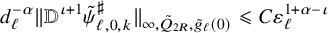 $$ \begin{align} d_{\ell}^{-\alpha}\|{\mathbb{D}}^{\iota+1}\tilde{\psi}^\sharp_{\ell,0,k}\|_{\infty,\tilde{Q}_{2R},\tilde{g}_{\ell}(0)}\leqslant C\varepsilon_{\ell}^{1+\alpha-\iota} \end{align} $$
for the first term in the last line of (4.245). As for the other term in that line, it is only nontrivial when
 $\iota =p=q=0$
, and in that case, we want to bound
$\iota =p=q=0$
, and in that case, we want to bound
 $d_{\ell }^{-\alpha }\|\partial _{\tilde {t}}\tilde {\psi }^\sharp _{\ell ,0,k}\|_{\infty ,\tilde {Q}_{2R},\tilde {g}_{\ell }(0)}$
. Since we have
$d_{\ell }^{-\alpha }\|\partial _{\tilde {t}}\tilde {\psi }^\sharp _{\ell ,0,k}\|_{\infty ,\tilde {Q}_{2R},\tilde {g}_{\ell }(0)}$
. Since we have
 $\partial _{\tilde {t}}\tilde {\psi }^\sharp _{\ell ,0,k}=(\partial _{\tilde {t}}\tilde {\psi }_{\ell ,0,k})(\tilde {\mathbf {x}}_{\ell },\tilde {t}_{\ell })$
, we obtain from (4.244)
$\partial _{\tilde {t}}\tilde {\psi }^\sharp _{\ell ,0,k}=(\partial _{\tilde {t}}\tilde {\psi }_{\ell ,0,k})(\tilde {\mathbf {x}}_{\ell },\tilde {t}_{\ell })$
, we obtain from (4.244)
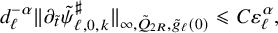 $$ \begin{align} d_{\ell}^{-\alpha}\|\partial_{\tilde{t}}\tilde{\psi}^\sharp_{\ell,0,k}\|_{\infty,\tilde{Q}_{2R},\tilde{g}_{\ell}(0)}\leqslant C\varepsilon_{\ell}^{\alpha}, \end{align} $$
and combining (4.245) with (4.251) and (4.252) proves (4.241).
To prove (4.242), given
 $p,q\geqslant 0$
with
$p,q\geqslant 0$
with
 $p+2q=\iota $
, to bound
$p+2q=\iota $
, to bound
 $d_{\ell }^{-\alpha }{\mathbb {D}}^p\partial _{\tilde {t}}^q\tilde {\psi }^\sharp _{\ell ,0,k}$
, we again need to consider only two cases. The first case (
$d_{\ell }^{-\alpha }{\mathbb {D}}^p\partial _{\tilde {t}}^q\tilde {\psi }^\sharp _{\ell ,0,k}$
, we again need to consider only two cases. The first case (
 $q=0,p=\iota $
) is the one with only spatial derivatives that land on the spatial Taylor polynomial (writing again
$q=0,p=\iota $
) is the one with only spatial derivatives that land on the spatial Taylor polynomial (writing again
 $\psi =d_{\ell }^{-\alpha }\tilde {\psi }_{\ell ,0,k}$
)
$\psi =d_{\ell }^{-\alpha }\tilde {\psi }_{\ell ,0,k}$
)
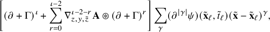 $$ \begin{align} \left[(\partial + \Gamma)^\iota+ \sum_{r=0}^{\iota-2}\nabla_{z,y,\tilde{z}}^{\iota-2-r}\mathbf{A}\circledast(\partial+\Gamma)^r\right]\sum_\gamma(\partial^{|\gamma|}\psi)(\tilde{\mathbf{x}}_{\ell},\tilde{t}_{\ell}) (\tilde{\mathbf{x}}-\tilde{\mathbf{x}}_{\ell})^\gamma, \end{align} $$
whose
 $L^\infty $
norm on
$L^\infty $
norm on
 $\tilde {Q}_{2R}$
is bounded by
$\tilde {Q}_{2R}$
is bounded by
 $C\varepsilon _{\ell }^{2+\alpha -\iota }$
thanks to the estimates in Step (3) (with
$C\varepsilon _{\ell }^{2+\alpha -\iota }$
thanks to the estimates in Step (3) (with
 $r=\iota $
) and Step (4) (with
$r=\iota $
) and Step (4) (with
 $\iota $
there replaced by
$\iota $
there replaced by
 $\iota -1$
). The second case only happens when
$\iota -1$
). The second case only happens when
 $\iota =2$
and we have only 1 time derivative that lands on the
$\iota =2$
and we have only 1 time derivative that lands on the
 $\tilde {t}$
-variable Taylor polynomial, which gives simply
$\tilde {t}$
-variable Taylor polynomial, which gives simply
 $d_{\ell }^{-\alpha }(\partial _{\tilde {t}}\tilde {\psi }_{\ell ,0,k})(\tilde {\mathbf {x}}_{\ell },\tilde {t}_{\ell })$
, and this is bounded by
$d_{\ell }^{-\alpha }(\partial _{\tilde {t}}\tilde {\psi }_{\ell ,0,k})(\tilde {\mathbf {x}}_{\ell },\tilde {t}_{\ell })$
, and this is bounded by
 $C\varepsilon _{\ell }^{\alpha }$
by (4.244). Putting these observations together proves (4.242).
$C\varepsilon _{\ell }^{\alpha }$
by (4.244). Putting these observations together proves (4.242).
Combining (4.241) for
 $\iota =2$
with the bound
$\iota =2$
with the bound
 $d_{\ell }^{-\alpha }[\mathfrak {D}^2\tilde {\psi }_{\ell ,0,k}]_{{\alpha },{\alpha }/2,\tilde {Q}_{R},\tilde {g}_{\ell }(0)}\leqslant C$
from (4.144), we see that
$d_{\ell }^{-\alpha }[\mathfrak {D}^2\tilde {\psi }_{\ell ,0,k}]_{{\alpha },{\alpha }/2,\tilde {Q}_{R},\tilde {g}_{\ell }(0)}\leqslant C$
from (4.144), we see that
 $$ \begin{align} d_{\ell}^{-\alpha}[\mathfrak{D}^2\tilde{\psi}^{*}_{\ell,0,k}]_{{\alpha},{\alpha}/2,\tilde{Q}_{R},\tilde{g}_{\ell}(0)}\leqslant C_R, \end{align} $$
and so we can apply Lemma 2.4 and get
 $$ \begin{align} d_{\ell}^{-\alpha}\|\mathfrak{D}^\iota\tilde{\psi}^{*}_{\ell,0,k}\|_{\infty,\tilde{Q}_{R},\tilde{g}_{\ell}(0)}\leqslant C_R,\quad d_{\ell}^{-\alpha}[\mathfrak{D}^\iota\tilde{\psi}^{*}_{\ell,0,k}]_{{\alpha},{\alpha}/2,\tilde{Q}_{R},\tilde{g}_{\ell}(0)}\leqslant C_R, \quad 0\leqslant\iota\leqslant 2. \end{align} $$
However, from (4.153), we also get uniform local parabolic
 $C^{{\alpha },{\alpha }/2}$
bounds on
$C^{{\alpha },{\alpha }/2}$
bounds on
 $d_{\ell }^{-\alpha }e^{-d_{\ell }^2\lambda _{\ell }^{-2}\tilde t}\partial _{\tilde {t}}\underline{\tilde \chi _{\ell }^{*}}$
and
$d_{\ell }^{-\alpha }e^{-d_{\ell }^2\lambda _{\ell }^{-2}\tilde t}\partial _{\tilde {t}}\underline{\tilde \chi _{\ell }^{*}}$
and
 $d_{\ell }^{-\alpha }{i\partial \bar \partial }\left(e^{-d_{\ell }^2\lambda _{\ell }^{-2}\tilde t}\underline{\tilde \chi _{\ell }^{*} }\right)$
, and so if we define
$d_{\ell }^{-\alpha }{i\partial \bar \partial }\left(e^{-d_{\ell }^2\lambda _{\ell }^{-2}\tilde t}\underline{\tilde \chi _{\ell }^{*} }\right)$
, and so if we define
 $$ \begin{align} \tilde{\rho}^{*}_{\ell}:=\tilde{\psi}^{*}_{\ell,0,k}+e^{-d_{\ell}^2\lambda_{\ell}^{-2}\tilde t}\underline{\tilde \chi_{\ell}^{*} }, \end{align} $$
then from (4.214), we have
 $\tilde {\rho }_{\ell }=\tilde {\rho }^{*}_{\ell }+\tilde {\psi }^\sharp _{\ell ,0,k},$
and
$\tilde {\rho }_{\ell }=\tilde {\rho }^{*}_{\ell }+\tilde {\psi }^\sharp _{\ell ,0,k},$
and
 $$ \begin{align} d_{\ell}^{-\alpha}\left(\partial_{\tilde{t}}\tilde{\rho}^{*}_{\ell}+d_{\ell}^2\lambda_{\ell}^{-2}\tilde{\rho}^{*}_{\ell}\right)=d_{\ell}^{-\alpha}e^{-d_{\ell}^2\lambda_{\ell}^{-2}\tilde t}\partial_{\tilde{t}}\underline{\tilde \chi_{\ell}^{*}} +d_{\ell}^{-\alpha}\left(\partial_{\tilde{t}}\tilde{\psi}^{*}_{\ell,0,k}+d_{\ell}^2\lambda_{\ell}^{-2}\tilde{\psi}^{*}_{\ell,0,k}\right), \end{align} $$
which by these estimates has uniform local parabolic
 $C^{{\alpha },{\alpha }/2}$
bounds. The same estimates also give us uniform local parabolic
$C^{{\alpha },{\alpha }/2}$
bounds. The same estimates also give us uniform local parabolic
 $C^{{\alpha },{\alpha }/2}$
bounds on
$C^{{\alpha },{\alpha }/2}$
bounds on
 $d_{\ell }^{-\alpha }{i\partial \bar \partial }\tilde {\rho }^{*}_{\ell }$
, so passing to a subsequence, we have that
$d_{\ell }^{-\alpha }{i\partial \bar \partial }\tilde {\rho }^{*}_{\ell }$
, so passing to a subsequence, we have that
 $$ \begin{align} d_{\ell}^{-\alpha}\left(\partial_{\tilde{t}}\tilde{\rho}^{*}_{\ell}+d_{\ell}^2\lambda_{\ell}^{-2}\tilde{\rho}^{*}_{\ell}\right)\to u_\infty, \quad d_{\ell}^{-\alpha}{i\partial\bar\partial}\tilde{\rho}^{*}_{\ell}\to\eta_\infty, \end{align} $$
in
 $C^{\gamma ,\gamma /2}_{\mathrm {loc}}$
for all
$C^{\gamma ,\gamma /2}_{\mathrm {loc}}$
for all
 $0<\gamma <{\alpha }$
, for a function
$0<\gamma <{\alpha }$
, for a function
 $u_\infty \in C^{{\alpha },{\alpha }/2}_{\mathrm {loc}}$
and a
$u_\infty \in C^{{\alpha },{\alpha }/2}_{\mathrm {loc}}$
and a
 $(1,1)$
-form
$(1,1)$
-form
 $\eta _\infty \in C^{{\alpha },{\alpha }/2}_{\mathrm {loc}}$
on
$\eta _\infty \in C^{{\alpha },{\alpha }/2}_{\mathrm {loc}}$
on
 $\mathbb {C}^{m+n}\times (-\infty ,0]$
. Moreover, thanks to (4.157) and (4.255), we have
$\mathbb {C}^{m+n}\times (-\infty ,0]$
. Moreover, thanks to (4.157) and (4.255), we have
 $$ \begin{align} d_{\ell}^{-{\alpha}+2}\lambda_{\ell}^{-2}\|\tilde{\rho}^{*}_{\ell}\|_{\infty, \tilde{Q}_R}\leqslant C_Rd_{\ell}^2\lambda_{\ell}^{-2}+o(1)d_{\ell}^2=o(1), \end{align} $$
and hence,
 $d_{\ell }^{-\alpha }\partial _{\tilde {t}}\tilde {\rho }^{*}_{\ell }\to u_\infty $
locally uniformly.
$d_{\ell }^{-\alpha }\partial _{\tilde {t}}\tilde {\rho }^{*}_{\ell }\to u_\infty $
locally uniformly.
Next, we observe that by definition, for any fixed
 $R>0$
, we have
$R>0$
, we have
 $$ \begin{align} d_{\ell}^{-\alpha}[e^{-d_{\ell}^2\lambda_{\ell}^{-2}\tilde t} \partial_{\tilde t}\tilde \chi_{\ell} ]_{{\alpha},{\alpha}/2,\tilde Q_{R},\tilde g_{\ell}(0)}= d_{\ell}^{-\alpha}[\partial_{\tilde t}\tilde \varphi _{\ell}+d_{\ell}^2\lambda_{\ell}^{-2}\tilde \varphi _{\ell}]_{{\alpha},{\alpha}/2,\tilde Q_{R},\tilde g_{\ell}(0)} =[\partial_{\hat{t}}\hat{\varphi }_{\ell}+\lambda_{\ell}^{-2}\hat{\varphi }_{\ell}]_{{\alpha},{\alpha}/2,\hat{Q}_{R d_{\ell}},\hat{g}_{\ell}(0)}=o(1), \end{align} $$
thanks to (4.136), and similarly from (4.137),
 $$ \begin{align} d_{\ell}^{-\alpha}[e^{-d_{\ell}^2\lambda_{\ell}^{-2}\tilde t} \partial_{\tilde t}\underline{\tilde \chi_{\ell} } ]_{{\alpha},{\alpha}/2,\tilde Q_{R},\tilde g_{\ell}(0)} =[\partial_{\hat{t}}\underline{\hat{\varphi }_{\ell}}+\lambda_{\ell}^{-2}\underline{\hat{\varphi }_{\ell}}]_{{\alpha},{\alpha}/2,\hat{Q}_{R d_{\ell}},\hat{g}_{\ell}(0)}=o(1), \end{align} $$
and since
 $$ \begin{align} e^{-d_{\ell}^2\lambda_{\ell}^{-2}\tilde t} \partial_{\tilde t}\tilde \chi_{\ell}-e^{-d_{\ell}^2\lambda_{\ell}^{-2}\tilde t} \partial_{\tilde t}\underline{\tilde \chi_{\ell} }= \partial_{\tilde{t}}\tilde{\psi}_{\ell,0,k}+d_{\ell}^2\lambda_{\ell}^{-2}\tilde{\psi}_{\ell,0,k}, \end{align} $$
we see that
 $$ \begin{align} d_{\ell}^{-\alpha}[\partial_{\tilde{t}}\tilde{\psi}_{\ell,0,k}+d_{\ell}^2\lambda_{\ell}^{-2}\tilde{\psi}_{\ell,0,k}]_{{\alpha},{\alpha}/2,\tilde Q_{R},\tilde g_{\ell}(0)}=o(1), \end{align} $$
and using (4.144), this gives
 $$ \begin{align} d_{\ell}^{-\alpha}[\partial_{\tilde{t}}\tilde{\psi}_{\ell,0,k}]_{{\alpha},{\alpha}/2,\tilde Q_{R},\tilde g_{\ell}(0)}=o(1), \end{align} $$
which combined with (4.241) implies
 $$ \begin{align} d_{\ell}^{-\alpha}[\partial_{\tilde{t}}\tilde{\psi}^{*}_{\ell,0,k}]_{{\alpha},{\alpha}/2,\tilde Q_{R},\tilde g_{\ell}(0)}=o(1). \end{align} $$
Also, (4.255) implies that
 $$ \begin{align} d_{\ell}^{-\alpha}d_{\ell}^2\lambda_{\ell}^{-2}[\tilde{\psi}^{*}_{\ell,0,k}]_{{\alpha},{\alpha}/2,\tilde Q_{R},\tilde g_{\ell}(0)}=o(1). \end{align} $$
However, from (4.158), we see that
 $$ \begin{align} d_{\ell}^{-\alpha}[e^{-d_{\ell}^2\lambda_{\ell}^{-2}\tilde t} \partial_{\tilde t}\underline{\tilde \chi_{\ell}^\sharp } ]_{{\alpha},{\alpha}/2,\tilde Q_{R},\tilde g_{\ell}(0)}=o(1), \end{align} $$
and which combined with (4.261) gives
 $$ \begin{align} d_{\ell}^{-\alpha}[e^{-d_{\ell}^2\lambda_{\ell}^{-2}\tilde t} \partial_{\tilde t}\underline{\tilde \chi_{\ell}^{*} } ]_{{\alpha},{\alpha}/2,\tilde Q_{R},\tilde g_{\ell}(0)}=o(1). \end{align} $$
Plugging (4.265), (4.266) and (4.268) into (4.257) gives
 $$ \begin{align} d_{\ell}^{-\alpha}[\partial_{\tilde{t}}\tilde{\rho}^{*}_{\ell}+d_{\ell}^2\lambda_{\ell}^{-2}\tilde{\rho}^{*}_{\ell}]_{{\alpha},{\alpha}/2,\tilde Q_{R},\tilde g_{\ell}(0)}=o(1), \end{align} $$
which implies that
 $u_\infty $
is constant in space-time, and since its value at
$u_\infty $
is constant in space-time, and since its value at
 $(0,0)$
vanishes, we conclude that
$(0,0)$
vanishes, we conclude that
 $u_\infty \equiv 0$
on
$u_\infty \equiv 0$
on
 $\mathbb {C}^{m+n}\times (-\infty ,0]$
. Thus,
$\mathbb {C}^{m+n}\times (-\infty ,0]$
. Thus,
 $d_{\ell }^{-\alpha }\partial _{\tilde {t}}\tilde {\rho }^{*}_{\ell }\to 0$
locally uniformly.
$d_{\ell }^{-\alpha }\partial _{\tilde {t}}\tilde {\rho }^{*}_{\ell }\to 0$
locally uniformly.
Given any
 $(\tilde {x},\tilde {t}),(\tilde {x},\tilde {t}')\in \tilde {Q}_R$
, we have
$(\tilde {x},\tilde {t}),(\tilde {x},\tilde {t}')\in \tilde {Q}_R$
, we have
 $$ \begin{align} d_{\ell}^{-{\alpha}}{i\partial\bar\partial}\tilde{\rho}^{*}_{\ell}(\tilde{x},\tilde{t})-d_{\ell}^{-{\alpha}}{i\partial\bar\partial}\tilde{\rho}^{*}_{\ell}(\tilde{x},\tilde{t}')={i\partial\bar\partial} \int_{\tilde{t}'}^{\tilde{t}}\left(d_{\ell}^{-{\alpha}}\partial_{\tilde{t}}\tilde{\rho}^{*}_{\ell}\right)(\tilde{x},\tilde{s})d\tilde{s}, \end{align} $$
and since we know that
 $\int _{t'}^t\left(d_{\ell }^{-{\alpha }}\partial _{\tilde {t}}\tilde {\rho }^{*}_{\ell }\right)(\tilde {x},\tilde {s})d\tilde {s} \to 0$
locally uniformly (as a function of
$\int _{t'}^t\left(d_{\ell }^{-{\alpha }}\partial _{\tilde {t}}\tilde {\rho }^{*}_{\ell }\right)(\tilde {x},\tilde {s})d\tilde {s} \to 0$
locally uniformly (as a function of
 $\tilde {x}$
), it follows that the RHS of (4.270) converges to zero weakly as currents. Since the LHS of (4.270) converges in
$\tilde {x}$
), it follows that the RHS of (4.270) converges to zero weakly as currents. Since the LHS of (4.270) converges in
 $C^\gamma _{\mathrm {loc}}$
to
$C^\gamma _{\mathrm {loc}}$
to
 $\eta _\infty (\tilde {x},\tilde {t})-\eta _\infty (\tilde {x},\tilde {t}')$
, we conclude that this Hölder continuous
$\eta _\infty (\tilde {x},\tilde {t})-\eta _\infty (\tilde {x},\tilde {t}')$
, we conclude that this Hölder continuous
 $(1,1)$
-form (with
$(1,1)$
-form (with
 $\tilde {x}$
varying) is zero as a current, and hence, it is identically zero. This shows that
$\tilde {x}$
varying) is zero as a current, and hence, it is identically zero. This shows that
 $\eta _\infty $
is time-independent.
$\eta _\infty $
is time-independent.
From (4.216), we have
 $$ \begin{align} \left(\partial_{\tilde{t}}-\Delta_{\tilde{\omega}^\sharp_{\ell}}\right)\tilde{\rho}^{*}_{\ell} + d_{\ell}^2\lambda_{\ell}^{-2}\tilde{\rho}^{*}_{\ell}=\mathcal{E}_1+\mathcal{E}_2+\mathcal{E}_3-\left(\partial_{\tilde{t}}-\Delta_{\tilde{\omega}^\sharp_{\ell}}\right)\tilde{\psi}^\sharp_{\ell,0,k}-d_{\ell}^2\lambda_{\ell}^{-2}\tilde{\psi}^\sharp_{\ell,0,k}, \end{align} $$
and from (4.234) and (4.241), we see that applying
 $d_{\ell }^{-\alpha }[\cdot ]_{{\alpha },{\alpha }/2,\tilde {Q}_R,\tilde {g}_{\ell }(0)}$
to the RHS of (4.271), we get
$d_{\ell }^{-\alpha }[\cdot ]_{{\alpha },{\alpha }/2,\tilde {Q}_R,\tilde {g}_{\ell }(0)}$
to the RHS of (4.271), we get
 $o(1)$
as
$o(1)$
as
 $\ell \to +\infty $
. We can then multiply (4.271) by
$\ell \to +\infty $
. We can then multiply (4.271) by
 $d_{\ell }^{-\alpha }$
, and since the LHS converges in
$d_{\ell }^{-\alpha }$
, and since the LHS converges in
 $C^{\gamma ,\gamma /2}_{\mathrm {loc}}$
, we can pass to the limit (recalling that
$C^{\gamma ,\gamma /2}_{\mathrm {loc}}$
, we can pass to the limit (recalling that
 $u_\infty \equiv 0$
) and get
$u_\infty \equiv 0$
) and get
 $$ \begin{align} \operatorname{tr}_{g_{\mathbb{C}^{m+n}}}\eta_\infty=c, \end{align} $$
on
 $\mathbb {C}^{m+n}\times (-\infty ,0]$
, for some time-independent constant c. Since the value of the LHS of (4.272) at
$\mathbb {C}^{m+n}\times (-\infty ,0]$
, for some time-independent constant c. Since the value of the LHS of (4.272) at
 $(0,0)$
is zero, this forces
$(0,0)$
is zero, this forces
 $c=0$
; that is,
$c=0$
; that is,
 $$ \begin{align} \operatorname{tr}_{g_{\mathbb{C}^{m+n}}}\eta_\infty=0. \end{align} $$
Since the
 $C^{\gamma }_{\mathrm {loc}}$
form
$C^{\gamma }_{\mathrm {loc}}$
form
 $\eta _\infty $
is time-independent and weakly closed, it can be written as
$\eta _\infty $
is time-independent and weakly closed, it can be written as
 $\eta _\infty ={i\partial \bar \partial } v_\infty $
for some time-independent function
$\eta _\infty ={i\partial \bar \partial } v_\infty $
for some time-independent function
 $v_\infty \in C^{2+\gamma }_{\mathrm {loc}}(\mathbb {C}^{m+n})$
. From (4.273), we see that
$v_\infty \in C^{2+\gamma }_{\mathrm {loc}}(\mathbb {C}^{m+n})$
. From (4.273), we see that
 $\Delta _{g_{\mathbb {C}^{m+n}}}v_\infty =0$
, so
$\Delta _{g_{\mathbb {C}^{m+n}}}v_\infty =0$
, so
 $\eta _\infty $
is smooth by elliptic regularity, and passing to the limit (4.153) and (4.254), we see that
$\eta _\infty $
is smooth by elliptic regularity, and passing to the limit (4.153) and (4.254), we see that
 $|{i\partial \bar \partial } v_\infty |=O(|z|^{\alpha })$
. Thus, each component
$|{i\partial \bar \partial } v_\infty |=O(|z|^{\alpha })$
. Thus, each component
 $\partial _{\alpha } \partial _{\bar {\beta }}v_\infty $
of
$\partial _{\alpha } \partial _{\bar {\beta }}v_\infty $
of
 ${i\partial \bar \partial } v_\infty $
satisfies
${i\partial \bar \partial } v_\infty $
satisfies
 $\Delta _{g_{\mathbb {C}^{m+n}}} \partial _{\alpha } \partial _{\bar {\beta }}v_\infty =0$
and
$\Delta _{g_{\mathbb {C}^{m+n}}} \partial _{\alpha } \partial _{\bar {\beta }}v_\infty =0$
and
 $|\partial _{\alpha } \partial _{\bar {\beta }}v_\infty |=O(|z|^{\alpha })$
, so by the standard Liouville Theorem for harmonic functions, we have that
$|\partial _{\alpha } \partial _{\bar {\beta }}v_\infty |=O(|z|^{\alpha })$
, so by the standard Liouville Theorem for harmonic functions, we have that
 $\eta _\infty $
has constant coefficients, and hence, it vanishes identically since its value at
$\eta _\infty $
has constant coefficients, and hence, it vanishes identically since its value at
 $(0,0)$
is zero.
$(0,0)$
is zero.
This implies that
 $$ \begin{align} d_{\ell}^{-\alpha}{i\partial\bar\partial}\tilde{\rho}^{*}_{\ell}\to 0, \end{align} $$
locally uniformly on
 $\mathbb {C}^{m+n}\times (-\infty ,0]$
in the coordinates
$\mathbb {C}^{m+n}\times (-\infty ,0]$
in the coordinates
 $(\tilde {\mathbf {x}},\tilde {t})$
. Recall that, by definition, we have
$(\tilde {\mathbf {x}},\tilde {t})$
. Recall that, by definition, we have
 $$ \begin{align} \tilde{\varphi }_{\ell}=\tilde{\rho}^{*}_{\ell}+\tilde{\psi}^\sharp_{\ell,0,k}+e^{-d_{\ell}^2\lambda_{\ell}^{-2}\tilde t}\underline{\tilde \chi_{\ell}^\sharp}, \end{align} $$
and that
 $\underline{\tilde \chi _{\ell }^\sharp }$
is a polynomial on
$\underline{\tilde \chi _{\ell }^\sharp }$
is a polynomial on
 $\mathbb {C}^m$
of degree at most
$\mathbb {C}^m$
of degree at most
 $2$
, while
$2$
, while
 $\tilde {\psi }^\sharp _{\ell ,0,k}$
is a polynomial on
$\tilde {\psi }^\sharp _{\ell ,0,k}$
is a polynomial on
 $\mathbb {C}^{m+n}$
(in the
$\mathbb {C}^{m+n}$
(in the
 $(\tilde {\mathbf {x}},\tilde {t})$
coordinates) of degree at most
$(\tilde {\mathbf {x}},\tilde {t})$
coordinates) of degree at most
 $2$
. To convert
$2$
. To convert
 ${i\partial \bar \partial }$
into
${i\partial \bar \partial }$
into
 ${\mathbb {D}}$
-derivatives, schematically we have
${\mathbb {D}}$
-derivatives, schematically we have
 ${i\partial \bar \partial }=\tilde {J}_{\ell }\circledast {\mathbb {D}}^2+({\mathbb {D}}\tilde {J}_{\ell })\circledast {\mathbb {D}}$
, with the bounds (cf. [Reference Hein and Tosatti21, (4.304)])
${i\partial \bar \partial }=\tilde {J}_{\ell }\circledast {\mathbb {D}}^2+({\mathbb {D}}\tilde {J}_{\ell })\circledast {\mathbb {D}}$
, with the bounds (cf. [Reference Hein and Tosatti21, (4.304)])
 $$ \begin{align} \|{\mathbb{D}}^\iota \tilde{J}_{\ell}\|_{\infty,\tilde{Q}_{Rd_{\ell}^{-1}},\tilde{g}_{\ell}(0)}\leqslant C\varepsilon_{\ell}^{-\iota},\quad [{\mathbb{D}}^\iota \tilde{J}_{\ell}]_{{\alpha},{\alpha}/2,\tilde{Q}_{Rd_{\ell}^{-1}},\tilde{g}_{\ell}(0)}\leqslant C\varepsilon_{\ell}^{-\iota-{\alpha}}. \end{align} $$
Since
 $\tilde {J}_{\ell }$
and
$\tilde {J}_{\ell }$
and
 ${\mathbb {D}}$
are independent of
${\mathbb {D}}$
are independent of
 $\tilde {t}$
, it follows that
$\tilde {t}$
, it follows that
 $$ \begin{align} \partial_{\tilde{t}}{i\partial\bar\partial}\tilde{\psi}^\sharp_{\ell,0,k}=\tilde{J}_{\ell}\circledast{\mathbb{D}}^2\partial_{\tilde{t}}\tilde{\psi}^\sharp_{\ell,0,k}+({\mathbb{D}}\tilde{J}_{\ell})\circledast {\mathbb{D}}\partial_{\tilde{t}}\tilde{\psi}^\sharp_{\ell,0,k}=0, \end{align} $$
so, as in the proof of (4.245), we can bound
 $$ \begin{align} \begin{aligned} d_{\ell}^{-{\alpha}}[{i\partial\bar\partial}\tilde{\psi}^\sharp_{\ell,0,k}]_{{\alpha},{\alpha}/2,\tilde{Q}_{R},\tilde{g}_{\ell}(0)}&\leqslant CR^{1-\alpha}d_{\ell}^{-{\alpha}}\|{\mathbb{D}}{i\partial\bar\partial}\tilde{\psi}^\sharp_{\ell,0,k}\|_{\infty, \tilde{Q}_{2R},\tilde{g}_{\ell}(0)}\\&\leqslant CR^{1-\alpha}d_{\ell}^{-{\alpha}}\big(\|{\mathbb{D}}^3\tilde{\psi}^\sharp_{\ell,0,k}\|_{\infty, \tilde{Q}_{2R},\tilde{g}_{\ell}(0)}+\varepsilon_{\ell}^{-1}\|{\mathbb{D}}^2\tilde{\psi}^\sharp_{\ell,0,k}\|_{\infty, \tilde{Q}_{2R},\tilde{g}_{\ell}(0)}\\&\quad+\varepsilon_{\ell}^{-2}\|{\mathbb{D}}\tilde{\psi}^\sharp_{\ell,0,k}\|_{\infty, \tilde{Q}_{2R},\tilde{g}_{\ell}(0)}\big)\\&\leqslant CR^{1-\alpha}\varepsilon_{\ell}^{{\alpha}-2}=o(1), \end{aligned} \end{align} $$
using (4.276) for the second inequality and (4.242) for the third one. Also, from the bounds (4.158), it follows easily that
 $$ \begin{align} d_{\ell}^{-{\alpha}}\left[e^{-d_{\ell}^2\lambda_{\ell}^{-2}\tilde t}{i\partial\bar\partial}\underline{\tilde \chi_{\ell}^\sharp}\right]_{{\alpha},{\alpha}/2,\tilde{Q}_{R},\tilde{g}_{\ell}(0)}=o(1), \end{align} $$
and so using (4.274), (4.275), (4.278) and (4.279), and recalling also (4.112), we see that
 $$ \begin{align} d_{\ell}^{-{\alpha}}|{i\partial\bar\partial}\tilde{\varphi }_{\ell}(\tilde{x}_{\ell},0)-\mathbb{P}_{\tilde x^{\prime}_{\ell}\tilde x_{\ell}}{i\partial\bar\partial}\tilde{\varphi }_{\ell}(\tilde{x}_{\ell}^{\prime},\tilde{t}^{\prime}_{\ell})|_{\tilde{g}_{\ell}(0)}=o(1), \end{align} $$
a contradiction to (4.110).
4.12.2 The case
$j\geqslant 1$
. Killing the contribution of
$\tilde A_{\ell ,i,p,k}$


In the rest of this section, we will assume that
 $j\geqslant 1$
. The goal of this subsection is to prove a precise estimate on
$j\geqslant 1$
. The goal of this subsection is to prove a precise estimate on
 $\tilde A_{\ell ,i,p,k}$
: for all
$\tilde A_{\ell ,i,p,k}$
: for all
 $a\geqslant 2j$
,
$a\geqslant 2j$
,
 $a\in 2\mathbb {N}$
and
$a\in 2\mathbb {N}$
and
 ${\alpha }\leqslant {\beta }<1$
, there is
${\alpha }\leqslant {\beta }<1$
, there is
 $C>0$
such that
$C>0$
such that
 $$ \begin{align} d_{\ell}^{-2j-{\alpha}}\sum_{i=1}^j\sum_{p=1}^{N_{i,k}} \varepsilon_{\ell}^{a-2j-2}[\mathfrak{D}^a \tilde A^{*}_{\ell,i,p,k}]_{{\beta},{\beta}/2,\tilde Q_{O(\varepsilon_{\ell})},\tilde g_{\ell}(0)}\leqslant C \varepsilon_{\ell}^{{\alpha}-{\beta}}, \end{align} $$
where here and in the rest of this section, we use the notation
 $O(\varepsilon _{\ell })$
for a radius R such that
$O(\varepsilon _{\ell })$
for a radius R such that
 $\Lambda \varepsilon _{\ell } \leqslant R\leqslant \Lambda ^2\varepsilon _{\ell }$
, where
$\Lambda \varepsilon _{\ell } \leqslant R\leqslant \Lambda ^2\varepsilon _{\ell }$
, where
 $\Lambda>1$
is the fixed constant from (2.5) (so that the
$\Lambda>1$
is the fixed constant from (2.5) (so that the
 $\tilde {g}_{\ell }(0)$
-geodesic ball centered at
$\tilde {g}_{\ell }(0)$
-geodesic ball centered at
 $\tilde {x}_{\ell }$
with radius R contains a Euclidean ball of radius
$\tilde {x}_{\ell }$
with radius R contains a Euclidean ball of radius
 $R/2$
times the whole Y fiber). Note that since
$R/2$
times the whole Y fiber). Note that since
 $j\geqslant 1$
, we have
$j\geqslant 1$
, we have
 $a\geqslant 2$
.
$a\geqslant 2$
.
Observe that once (4.281) is established for all even
 $a\geqslant 2j$
, the same estimate will also hold for all
$a\geqslant 2j$
, the same estimate will also hold for all
 $a\geqslant 2j$
by interpolation: indeed, if
$a\geqslant 2j$
by interpolation: indeed, if
 $a\geqslant 2j+1$
is odd, then for any
$a\geqslant 2j+1$
is odd, then for any
 $0<\rho <R$
,
$0<\rho <R$
,
 $$ \begin{align} \begin{aligned} d_{\ell}^{-2j-{\alpha}}\varepsilon_{\ell}^{a-2j-2}[\mathfrak{D}^a \tilde A^{*}_{\ell,i,p,k}]_{{\beta},{\beta}/2,\tilde Q_{\rho},\tilde g_{\ell}(0)}&\leqslant C(R-\rho)d_{\ell}^{-2j-{\alpha}}\varepsilon_{\ell}^{a-2j-2}[\mathfrak{D}^{a+1} \tilde A^{*}_{\ell,i,p,k}]_{{\beta},{\beta}/2,\tilde Q_{R},\tilde g_{\ell}(0)}\\&\quad+C(R-\rho)^{-1}d_{\ell}^{-2j-{\alpha}}\varepsilon_{\ell}^{a-2j-2}[\mathfrak{D}^{a-1} \tilde A^{*}_{\ell,i,p,k}]_{{\beta},{\beta}/2,\tilde Q_{R},\tilde g_{\ell}(0)}\\&\leqslant C(R-\rho)\varepsilon_{\ell}^{\alpha-\beta-1}+C(R-\rho)^{-1}\varepsilon_{\ell}^{\alpha-\beta+1}, \end{aligned} \end{align} $$
and taking
 $\rho ,R=O(\varepsilon _{\ell })$
gives the claim.
$\rho ,R=O(\varepsilon _{\ell })$
gives the claim.
Thus, once (4.281) is established, taking
 $a=2j+2+\iota $
(with
$a=2j+2+\iota $
(with
 $-2\leqslant \iota \leqslant 2k$
), and
$-2\leqslant \iota \leqslant 2k$
), and
 $\beta>\alpha $
gives an
$\beta>\alpha $
gives an
 $o(1)$
bound for the
$o(1)$
bound for the
 $C^{\beta ,\beta /2}$
seminorm on the cylinder centered at
$C^{\beta ,\beta /2}$
seminorm on the cylinder centered at
 $(\tilde {x}_{\ell },\tilde {t}_{\ell })$
of radius
$(\tilde {x}_{\ell },\tilde {t}_{\ell })$
of radius
 $2$
, which contains the other blowup point
$2$
, which contains the other blowup point
 $(\tilde {x}^{\prime }_{\ell },\tilde {t}^{\prime }_{\ell })$
which lies at distance
$(\tilde {x}^{\prime }_{\ell },\tilde {t}^{\prime }_{\ell })$
which lies at distance
 $1$
, and hence an
$1$
, and hence an
 $o(1)$
bound for the
$o(1)$
bound for the
 $C^{\alpha ,\alpha /2}$
seminorm on the same cylinder, which kills the contribution of
$C^{\alpha ,\alpha /2}$
seminorm on the same cylinder, which kills the contribution of
 $\mathfrak {D}^{2j+2+\iota }\tilde A^{*}_{\ell ,i,p,k}$
in (4.132).
$\mathfrak {D}^{2j+2+\iota }\tilde A^{*}_{\ell ,i,p,k}$
in (4.132).
Apart from the fact that in our parabolic setting we only work with derivatives of even order (as was explained earlier), the overall argument to prove (4.281) will be similar to the one to prove [Reference Hein and Tosatti21, (4.252)], replacing
 ${\mathbb {D}}$
by
${\mathbb {D}}$
by
 $\mathfrak {D}$
, j by
$\mathfrak {D}$
, j by
 $2j$
and t by
$2j$
and t by
 $t_{\ell }$
. As in [Reference Hein and Tosatti21, (4.254)], we use (4.145), (4.153), (4.158), (4.191), (4.202) and Proposition 4.8 to conclude that for all
$t_{\ell }$
. As in [Reference Hein and Tosatti21, (4.254)], we use (4.145), (4.153), (4.158), (4.191), (4.202) and Proposition 4.8 to conclude that for all
 $a\geqslant 2j$
,
$a\geqslant 2j$
,
 $1\leqslant i\leqslant j, 1\leqslant p\leqslant N_{i,k}$
,
$1\leqslant i\leqslant j, 1\leqslant p\leqslant N_{i,k}$
,
 $a\in 2\mathbb {N}$
and
$a\in 2\mathbb {N}$
and
 ${\alpha }\leqslant {\beta }<1$
, there is
${\alpha }\leqslant {\beta }<1$
, there is
 $C>0$
so that
$C>0$
so that
 $$ \begin{align} \begin{aligned} &d_{\ell}^{-2j-{\alpha}}\varepsilon_{\ell}^{a-2j-2}[\mathfrak{D}^a\tilde A_{\ell,i,p,k}]_{{\beta},{\beta}/2,\tilde Q_{O(\varepsilon_{\ell})},\tilde g_{\ell}(0)}\\&\quad\leqslant o(\varepsilon_{\ell}^{{\alpha}-{\beta}})+ C \varepsilon_{\ell}^{a-2j}d_{\ell}^{-2j-{\alpha}} [\mathfrak{D}^a_{\textbf{bt}} \tilde \eta_{\ell}]_{{\beta},{\beta}/2,\mathrm{base},\tilde Q_{O(\varepsilon_{\ell})},\tilde g_{\ell}(0)}\\&\qquad +Ce^{-(1-{\beta})\frac{t_{\ell}}{2}} \sum_{b=2j+1}^a \lambda_{\ell}^{-{\beta}} \delta_{\ell}^{a-2j}d_{\ell}^{-b+{\beta}-{\alpha}}\|\mathfrak{D}^b(\tilde{\eta}_{\ell}^\circ+\tilde{\eta}_{\ell}^\diamondsuit+\tilde{\eta}_{\ell,j,k}) \|_{\infty,\tilde Q_{O(\varepsilon_{\ell})},\tilde g_{\ell}(0)}\\&\qquad +C\sum_{r=1}^{i-1}\sum_{q=1}^{N_{p,k}}\Big( d_{\ell}^{-2j-{\alpha}} \varepsilon_{\ell}^{2k+a-2j} [\mathfrak{D}^{a+2k+2}\tilde A_{\ell,r,q,k}]_{{\beta},{\beta}/2,\tilde Q_{O(\varepsilon_{\ell})},\tilde g_{\ell}(0)}\\&\qquad +\sum_{b=0}^{a+2k+2} d_{\ell}^{-2j-{\alpha}} \varepsilon_{\ell}^{a-2j-2} d_{\ell}^{a-b+{\beta}}e^{-(2k+2+1-{\beta})\frac{t_{\ell}}{2}} \lambda_{\ell}^{b-a-{\beta}} \|\mathfrak{D}^b \tilde A_{\ell,r,q,k}\|_{\infty,\tilde Q_{O(\varepsilon_{\ell})},\tilde g_{\ell}(0)} \Big). \end{aligned} \end{align} $$
Our goal is to show that each term on the right-hand side of (4.283) is of
 $O(\varepsilon _{\ell }^{{\alpha }-{\beta }})$
which implies (4.281).
$O(\varepsilon _{\ell }^{{\alpha }-{\beta }})$
which implies (4.281).
We first treat the second term,
 $[\mathfrak {D}^a_{\textbf {bt}} \tilde \eta _{\ell }]_{{\beta },{\beta }/2,\mathrm {base},\tilde Q_{O(\varepsilon _{\ell })},\tilde g_{\ell }(0)}$
. We start with noting that we can interchange
$[\mathfrak {D}^a_{\textbf {bt}} \tilde \eta _{\ell }]_{{\beta },{\beta }/2,\mathrm {base},\tilde Q_{O(\varepsilon _{\ell })},\tilde g_{\ell }(0)}$
. We start with noting that we can interchange
 $\tilde {\eta }_{\ell }$
with
$\tilde {\eta }_{\ell }$
with
 $\tilde {\eta }_{\ell }^\circ +\tilde {\eta }_{\ell }^\diamondsuit +\tilde {\eta }_{\ell ,j,k}$
thanks to (4.160) and (4.201): for all
$\tilde {\eta }_{\ell }^\circ +\tilde {\eta }_{\ell }^\diamondsuit +\tilde {\eta }_{\ell ,j,k}$
thanks to (4.160) and (4.201): for all
 $a\geqslant 2j$
,
$a\geqslant 2j$
,
 $a\in 2\mathbb {N}$
,
$a\in 2\mathbb {N}$
,
 $$ \begin{align} \varepsilon_{\ell}^{a-2j}d_{\ell}^{-2j-{\alpha}} [\mathfrak{D}^a_{\textbf{bt}} \tilde{\eta}_{\ell}]_{{\beta},{\beta}/2,\mathrm{base},\tilde Q_{O(\varepsilon_{\ell})},\tilde g_{\ell}(0)} \leqslant \varepsilon_{\ell}^{a-2j}d_{\ell}^{-2j-{\alpha}} [\mathfrak{D}^a (\tilde \eta_{\ell,j,k}+\tilde \eta_{\ell}^\diamondsuit+\tilde{\eta}_{\ell}^\circ)]_{{\beta},{\beta}/2,\tilde Q_{O(\varepsilon_{\ell})},\tilde g_{\ell}(0)}+o(\varepsilon_{\ell}^{{\alpha}-{\beta}}). \end{align} $$
To bound the RHS of (4.284) using the parabolic Schauder estimates in Proposition 2.9, we need to pass to the check picture via the diffeomorphism
 $$ \begin{align} \Pi_{\ell}: B_{e^{\frac{t_{\ell}}{2}}}\times Y\times[-e^{t_{\ell}}t_{\ell},0] \to B_{d_{\ell}^{-1}\lambda_{\ell}}\times Y\times [-d_{\ell}^{-2}\lambda_{\ell}^2t_{\ell},0], \;\, (\tilde{z},\tilde{y},\tilde{t}) = \Pi_{\ell}(\check{z},\check{y},\check{t}) =(\varepsilon_{\ell}\check{z},\check{y},\varepsilon_{\ell}^2\check{t}), \end{align} $$
pulling back all geometric quantities and scaling
 $2$
-forms by
$2$
-forms by
 $\varepsilon _{\ell }^{-2}$
. We can then apply Proposition 2.9 to
$\varepsilon _{\ell }^{-2}$
. We can then apply Proposition 2.9 to
 $\check \eta _{\ell ,j,k}+\check \eta _{\ell }^\diamondsuit +\check \eta _{\ell }^\circ $
and then transfer the result back to the tilde picture. This shows that given any radius
$\check \eta _{\ell ,j,k}+\check \eta _{\ell }^\diamondsuit +\check \eta _{\ell }^\circ $
and then transfer the result back to the tilde picture. This shows that given any radius
 $R=O(\varepsilon _{\ell })$
and
$R=O(\varepsilon _{\ell })$
and
 $0<\rho <R$
, and letting
$0<\rho <R$
, and letting
 $\tilde {R}=\rho +\frac {1}{2}(R-\rho )$
, we have
$\tilde {R}=\rho +\frac {1}{2}(R-\rho )$
, we have
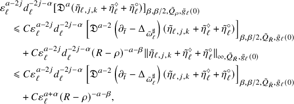 $$ \begin{align} \begin{aligned} &\varepsilon_{\ell}^{a-2j}d_{\ell}^{-2j-{\alpha}} [\mathfrak{D}^a (\tilde \eta_{\ell,j,k}+\tilde \eta_{\ell}^\diamondsuit+\tilde{\eta}_{\ell}^\circ)]_{{\beta},{\beta}/2,\tilde Q_{\rho},\tilde g_{\ell}(0)}\\&\quad \leqslant C\varepsilon_{\ell}^{a-2j}d_{\ell}^{-2j-{\alpha}} \left[\mathfrak{D}^{a-2}\left(\partial_{\tilde{t}}-\Delta_{\tilde{\omega}_{\ell}^\sharp}\right)(\tilde \eta_{\ell,j,k}+\tilde \eta_{\ell}^\diamondsuit+\tilde{\eta}_{\ell}^\circ)\right]_{{\beta},{\beta}/2,\tilde Q_{\tilde{R}},\tilde g_{\ell}(0)}\\&\qquad+C\varepsilon_{\ell}^{a-2j}d_{\ell}^{-2j-{\alpha}}(R-\rho)^{-a-\beta}\|\tilde \eta_{\ell,j,k}+\tilde \eta_{\ell}^\diamondsuit+\tilde{\eta}_{\ell}^\circ\|_{\infty,\tilde Q_{\tilde{R}},\tilde g_{\ell}(0)}\\&\quad\leqslant C\varepsilon_{\ell}^{a-2j}d_{\ell}^{-2j-{\alpha}} \left[\mathfrak{D}^{a-2}\left(\partial_{\tilde{t}}-\Delta_{\tilde{\omega}_{\ell}^\sharp}\right)(\tilde \eta_{\ell,j,k}+\tilde \eta_{\ell}^\diamondsuit+\tilde{\eta}_{\ell}^\circ)\right]_{{\beta},{\beta}/2,\tilde Q_{\tilde{R}},\tilde g_{\ell}(0)}\\&\qquad+C\varepsilon_{\ell}^{a+\alpha}(R-\rho)^{-a-\beta}, \end{aligned} \end{align} $$
using (4.145), (4.159) and (4.191), where here
 $\Delta _{\tilde {\omega }_{\ell }^\sharp }$
denotes the Hodge Laplacian acting on forms. This is the parabolic analog of [Reference Hein and Tosatti21, (4.259)]. Recalling that
$\Delta _{\tilde {\omega }_{\ell }^\sharp }$
denotes the Hodge Laplacian acting on forms. This is the parabolic analog of [Reference Hein and Tosatti21, (4.259)]. Recalling that
 $\tilde \eta _{\ell ,j,k}+\tilde \eta _{\ell }^\diamondsuit +\tilde {\eta }_{\ell }^\circ ={i\partial \bar \partial }\tilde {\rho }_{\ell },$
and using that the Hodge Laplacian of a Kähler metric commutes with
$\tilde \eta _{\ell ,j,k}+\tilde \eta _{\ell }^\diamondsuit +\tilde {\eta }_{\ell }^\circ ={i\partial \bar \partial }\tilde {\rho }_{\ell },$
and using that the Hodge Laplacian of a Kähler metric commutes with
 ${i\partial \bar \partial }$
, we have
${i\partial \bar \partial }$
, we have
 $$ \begin{align} \begin{aligned} &\left[\mathfrak{D}^{a-2}\left(\partial_{\tilde{t}}-\Delta_{\tilde{\omega}_{\ell}^\sharp}\right)(\tilde \eta_{\ell,j,k}+\tilde \eta_{\ell}^\diamondsuit+\tilde{\eta}_{\ell}^\circ)\right]_{{\beta},{\beta}/2,\tilde Q_{\tilde{R}},\tilde g_{\ell}(0)}=\left[\mathfrak{D}^{a-2}{i\partial\bar\partial}\left(\partial_{\tilde{t}}-\Delta_{\tilde{\omega}_{\ell}^\sharp}\right)\tilde{\rho}_{\ell}\right]_{{\beta},{\beta}/2,\tilde Q_{\tilde{R}},\tilde g_{\ell}(0)}, \end{aligned} \end{align} $$
and using the PDE (4.216), the triangle inequality and the boundedness of
 $\mathbb {P}$
-parallel transport, this can be bounded by
$\mathbb {P}$
-parallel transport, this can be bounded by
 $$ \begin{align} Cd_{\ell}^2\lambda_{\ell}^{-2}\left[\mathfrak{D}^{a-2}(\tilde \eta_{\ell,j,k}+\tilde \eta_{\ell}^\diamondsuit+\tilde{\eta}_{\ell}^\circ)\right]_{{\beta},{\beta}/2,\tilde Q_{\tilde{R}},\tilde g_{\ell}(0)} +C\left[\mathfrak{D}^{a-2}{i\partial\bar\partial}(\mathcal{E}_1+\mathcal{E}_2+\mathcal{E}_3)\right]_{{\beta},{\beta}/2,\tilde Q_{\tilde{R}},\tilde g_{\ell}(0)}, \end{align} $$
and inserting these into (4.286) and interpolating again with Proposition 2.3, we get
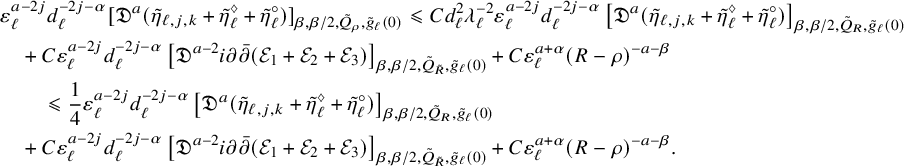 $$ \begin{align} \begin{aligned} &\varepsilon_{\ell}^{a-2j}d_{\ell}^{-2j-{\alpha}} [\mathfrak{D}^a (\tilde \eta_{\ell,j,k}+\tilde \eta_{\ell}^\diamondsuit+\tilde{\eta}_{\ell}^\circ)]_{{\beta},{\beta}/2,\tilde Q_{\rho},\tilde g_{\ell}(0)} \leqslant Cd_{\ell}^2\lambda_{\ell}^{-2}\varepsilon_{\ell}^{a-2j}d_{\ell}^{-2j-{\alpha}} \left[\mathfrak{D}^{a}(\tilde \eta_{\ell,j,k}+\tilde \eta_{\ell}^\diamondsuit+\tilde{\eta}_{\ell}^\circ)\right]_{{\beta},{\beta}/2,\tilde Q_{R},\tilde g_{\ell}(0)}\\&\quad+C\varepsilon_{\ell}^{a-2j}d_{\ell}^{-2j-{\alpha}}\left[\mathfrak{D}^{a-2}{i\partial\bar\partial}(\mathcal{E}_1+\mathcal{E}_2+\mathcal{E}_3)\right]_{{\beta},{\beta}/2,\tilde Q_{\tilde{R}},\tilde g_{\ell}(0)}+C\varepsilon_{\ell}^{a+\alpha}(R-\rho)^{-a-\beta}\\&\qquad\leqslant \frac{1}{4}\varepsilon_{\ell}^{a-2j}d_{\ell}^{-2j-{\alpha}} \left[\mathfrak{D}^{a}(\tilde \eta_{\ell,j,k}+\tilde \eta_{\ell}^\diamondsuit+\tilde{\eta}_{\ell}^\circ)\right]_{{\beta},{\beta}/2,\tilde Q_{R},\tilde g_{\ell}(0)}\\&\quad+C\varepsilon_{\ell}^{a-2j}d_{\ell}^{-2j-{\alpha}}\left[\mathfrak{D}^{a-2}{i\partial\bar\partial}(\mathcal{E}_1+\mathcal{E}_2+\mathcal{E}_3)\right]_{{\beta},{\beta}/2,\tilde Q_{\tilde{R}},\tilde g_{\ell}(0)}+C\varepsilon_{\ell}^{a+\alpha}(R-\rho)^{-a-\beta}. \end{aligned} \end{align} $$
The main claim is then the following:
Claim 4.9. For all
 $a\geqslant 2j$
,
$a\geqslant 2j$
,
 $a\in 2\mathbb {N}$
,
$a\in 2\mathbb {N}$
,
 $R=O(\varepsilon _{\ell })$
,
$R=O(\varepsilon _{\ell })$
,
 $0<\rho <R$
,
$0<\rho <R$
,
 ${\alpha }\leqslant {\beta }<1$
, if we let
${\alpha }\leqslant {\beta }<1$
, if we let
 $\tilde {R}=\rho +\frac {1}{2}(R-\rho )$
, then we have
$\tilde {R}=\rho +\frac {1}{2}(R-\rho )$
, then we have
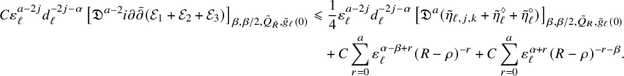 $$ \begin{align} \begin{aligned} C\varepsilon_{\ell}^{a-2j}d_{\ell}^{-2j-{\alpha}}\left[\mathfrak{D}^{a-2}{i\partial\bar\partial}(\mathcal{E}_1+\mathcal{E}_2+\mathcal{E}_3)\right]_{{\beta},{\beta}/2,\tilde Q_{\tilde{R}},\tilde g_{\ell}(0)}&\leqslant \frac{1}{4}\varepsilon_{\ell}^{a-2j}d_{\ell}^{-2j-{\alpha}} \left[\mathfrak{D}^{a}(\tilde \eta_{\ell,j,k}+\tilde \eta_{\ell}^\diamondsuit+\tilde{\eta}_{\ell}^\circ)\right]_{{\beta},{\beta}/2,\tilde Q_{R},\tilde g_{\ell}(0)}\\&\quad+ C\sum_{r=0}^a \varepsilon_{\ell}^{{\alpha}-{\beta}+r}(R-\rho)^{-r}+C\sum_{r=0}^{a}\varepsilon_{\ell}^{{\alpha}+r} (R-\rho)^{-r-\beta}. \end{aligned} \end{align} $$
Before giving the proof of Claim 4.9, we establish some of its consequences. Suppose Claim 4.9 has been proved for some
 $a\geqslant 2j$
. Then plugging it into (4.289) we get for all
$a\geqslant 2j$
. Then plugging it into (4.289) we get for all
 $R=O(\varepsilon _{\ell })$
and
$R=O(\varepsilon _{\ell })$
and
 $0<\rho <R$
,
$0<\rho <R$
,
 $$ \begin{align} \begin{aligned} \varepsilon_{\ell}^{a-2j}d_{\ell}^{-2j-{\alpha}} [\mathfrak{D}^a (\tilde \eta_{\ell,j,k}+\tilde \eta_{\ell}^\diamondsuit+\tilde{\eta}_{\ell}^\circ)]_{{\beta},{\beta}/2,\tilde Q_{\rho},\tilde g_{\ell}(0)} &\leqslant\frac{1}{2}\varepsilon_{\ell}^{a-2j}d_{\ell}^{-2j-{\alpha}} \left[\mathfrak{D}^{a}(\tilde \eta_{\ell,j,k}+\tilde \eta_{\ell}^\diamondsuit+\tilde{\eta}_{\ell}^\circ)\right]_{{\beta},{\beta}/2,\tilde Q_{R},\tilde g_{\ell}(0)}\\&\quad+C{\kern-1pt}\sum_{r=0}^a \varepsilon_{\ell}^{{\alpha}-{\beta}+r}(R-\rho)^{-r}+C{\kern-1pt}\sum_{r=0}^{a}\varepsilon_{\ell}^{{\alpha}+r} (R-\rho)^{-r-\beta}, \end{aligned} \end{align} $$
and then the iteration lemma in [Reference Hein and Tosatti21, Lemma 2.9] gives
 $$ \begin{align} \varepsilon_{\ell}^{a-2j}d_{\ell}^{-2j-{\alpha}} [\mathfrak{D}^a (\tilde \eta_{\ell,j,k}+\tilde \eta_{\ell}^\diamondsuit+\tilde{\eta}_{\ell}^\circ)]_{{\beta},{\beta}/2,\tilde Q_{\rho},\tilde g_{\ell}(0)} \leqslant C\sum_{r=0}^a \varepsilon_{\ell}^{{\alpha}-{\beta}+r}(R-\rho)^{-r}+C\sum_{r=0}^{a}\varepsilon_{\ell}^{{\alpha}+r} (R-\rho)^{-r-\beta}, \end{align} $$
and choosing now
 $\rho =O(\varepsilon _{\ell })$
gives
$\rho =O(\varepsilon _{\ell })$
gives
 $$ \begin{align} \varepsilon_{\ell}^{a-2j}d_{\ell}^{-2j-{\alpha}} [\mathfrak{D}^a (\tilde \eta_{\ell,j,k}+\tilde \eta_{\ell}^\diamondsuit+\tilde{\eta}_{\ell}^\circ)]_{{\beta},{\beta}/2,\tilde Q_{O(\varepsilon_{\ell})},\tilde g_{\ell}(0)} \leqslant C\varepsilon_{\ell}^{{\alpha}-\beta}, \end{align} $$
and this can be inserted back into (4.284) to finally give
 $$ \begin{align} \begin{aligned} \varepsilon_{\ell}^{a-2j}d_{\ell}^{-2j-{\alpha}} [\mathfrak{D}^a_{ \textbf{bt}}\tilde{\eta}_{\ell}]_{{\beta},{\beta}/2,\mathrm{base},\tilde Q_{O(\varepsilon_{\ell})},\tilde g_{\ell}(0)} &\leqslant C\varepsilon_{\ell}^{{\alpha}-{\beta}}, \end{aligned} \end{align} $$
which would show that the second term on the RHS of (4.283) is
 $O(\varepsilon _{\ell }^{{\alpha }-{\beta }})$
.
$O(\varepsilon _{\ell }^{{\alpha }-{\beta }})$
.
Furthermore, we can interpolate between (4.293) and the
 $L^\infty $
norm bound for
$L^\infty $
norm bound for
 $\tilde \eta _{\ell ,j,k}+\tilde \eta _{\ell }^\diamondsuit +\tilde {\eta }_{\ell }^\circ $
that comes from (4.145), (4.159) and (4.191), using Proposition 2.3 on cylinders of radius
$\tilde \eta _{\ell ,j,k}+\tilde \eta _{\ell }^\diamondsuit +\tilde {\eta }_{\ell }^\circ $
that comes from (4.145), (4.159) and (4.191), using Proposition 2.3 on cylinders of radius
 $O(\varepsilon _{\ell })$
to see that
$O(\varepsilon _{\ell })$
to see that
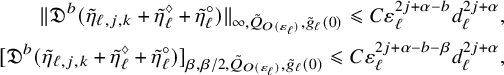
for all
 $0\leqslant b\leqslant a$
, and so following the discussion in [Reference Hein and Tosatti21, (4.280)–(4.283)], this implies that the third term on the RHS of (4.283) is of
$0\leqslant b\leqslant a$
, and so following the discussion in [Reference Hein and Tosatti21, (4.280)–(4.283)], this implies that the third term on the RHS of (4.283) is of
 $O(\varepsilon _{\ell }^{{\alpha }-{\beta }})$
.
$O(\varepsilon _{\ell }^{{\alpha }-{\beta }})$
.
To summarize, we have shown that if Claim 4.9 holds, then for all
 $a\geqslant 2j$
,
$a\geqslant 2j$
,
 $a\in 2\mathbb {N}$
,
$a\in 2\mathbb {N}$
,
 ${\alpha }\leqslant {\beta }<1$
,
${\alpha }\leqslant {\beta }<1$
,
 $1\leqslant i\leqslant j$
and
$1\leqslant i\leqslant j$
and
 $1\leqslant p\leqslant N_{i,k}$
, there is
$1\leqslant p\leqslant N_{i,k}$
, there is
 $C>0$
such that
$C>0$
such that
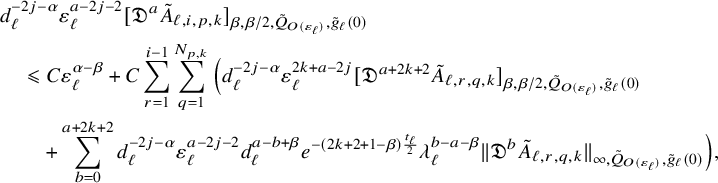 $$ \begin{align} \begin{aligned} &d_{\ell}^{-2j-{\alpha}}\varepsilon_{\ell}^{a-2j-2}[\mathfrak{D}^a\tilde A_{\ell,i,p,k}]_{{\beta},{\beta}/2,\tilde Q_{O(\varepsilon_{\ell})},\tilde g_{\ell}(0)}\\&\quad\leqslant C\varepsilon_{\ell}^{{\alpha}-{\beta}} +C\sum_{r=1}^{i-1}\sum_{q=1}^{N_{p,k}}\Big( d_{\ell}^{-2j-{\alpha}} \varepsilon_{\ell}^{2k+a-2j} [\mathfrak{D}^{a+2k+2}\tilde A_{\ell,r,q,k}]_{{\beta},{\beta}/2,\tilde Q_{O(\varepsilon_{\ell})},\tilde g_{\ell}(0)}\\&\quad \quad +\sum_{b=0}^{a+2k+2} d_{\ell}^{-2j-{\alpha}} \varepsilon_{\ell}^{a-2j-2} d_{\ell}^{a-b+{\beta}}e^{-(2k+2+1-{\beta})\frac{t_{\ell}}{2}} \lambda_{\ell}^{b-a-{\beta}} \|\mathfrak{D}^b \tilde A_{\ell,r,q,k}\|_{\infty,\tilde Q_{O(\varepsilon_{\ell})},\tilde g_{\ell}(0)} \Big), \end{aligned} \end{align} $$
which is the parabolic analog of [Reference Hein and Tosatti21, (4.283)]. The remaining argument follows closely that of [Reference Hein and Tosatti21, §4.10.5]. We use induction on
 $1\leqslant i\leqslant j$
to show that for all
$1\leqslant i\leqslant j$
to show that for all
 $a\geqslant 2j$
and
$a\geqslant 2j$
and
 $a\in 2\mathbb {N}$
, we have
$a\in 2\mathbb {N}$
, we have
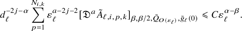 $$ \begin{align} d_{\ell}^{-2j-{\alpha}} \sum_{p=1}^{N_{i,k}} \varepsilon_{\ell}^{a-2j-2}[\mathfrak{D}^a \tilde A_{\ell,i,p,k}]_{{\beta},{\beta}/2,\tilde Q_{O(\varepsilon_{\ell})},\tilde g_{\ell}(0)}\leqslant C \varepsilon_{\ell}^{{\alpha}-{\beta}}. \end{align} $$
The base case
 $i=1$
follows directly from (4.296). Suppose (4.297) holds up to
$i=1$
follows directly from (4.296). Suppose (4.297) holds up to
 $i_0-1$
for some
$i_0-1$
for some
 $i_0\geqslant 2$
. Then the first term inside the summation on (4.296) can be estimated by
$i_0\geqslant 2$
. Then the first term inside the summation on (4.296) can be estimated by
 $C\varepsilon _{\ell }^{{\alpha }-{\beta }}$
since
$C\varepsilon _{\ell }^{{\alpha }-{\beta }}$
since
 $a+2k+2\in 2\mathbb {N}$
. We now treat the second term inside the summation – namely, the last line of (4.296). First, we treat the terms with
$a+2k+2\in 2\mathbb {N}$
. We now treat the second term inside the summation – namely, the last line of (4.296). First, we treat the terms with
 $0\leqslant b\leqslant 2j$
, by using (4.73) and transferring it to the tilde picture which gives
$0\leqslant b\leqslant 2j$
, by using (4.73) and transferring it to the tilde picture which gives
 $$ \begin{align} d_{\ell}^{-b}\| \mathfrak{D}^b \tilde A_{\ell,i,p,k}\|_{\infty,\tilde Q_{O(\varepsilon_{\ell})} , \tilde g_{\ell}(0)} =o(\varepsilon_{\ell}^{2}), \end{align} $$
and using these, we can bound these terms by
 $o(\varepsilon _{\ell }^{{\alpha }-{\beta }})$
exactly as in [Reference Hein and Tosatti21, (4.286)]. As for the terms with
$o(\varepsilon _{\ell }^{{\alpha }-{\beta }})$
exactly as in [Reference Hein and Tosatti21, (4.286)]. As for the terms with
 $2j<b\leqslant a+2k+2$
, we apply interpolation (i.e., Proposition 2.3) using (4.298) and (4.297) for
$2j<b\leqslant a+2k+2$
, we apply interpolation (i.e., Proposition 2.3) using (4.298) and (4.297) for
 $i\leqslant i_0-1$
from the induction hypothesis to show that for
$i\leqslant i_0-1$
from the induction hypothesis to show that for
 $2j<b\leqslant a+2k+2$
and
$2j<b\leqslant a+2k+2$
and
 $i\leqslant i_0-1$
,
$i\leqslant i_0-1$
,
 $$ \begin{align} \| \mathfrak{D}^b \tilde A_{\ell,i,p,k}\|_{\infty,\tilde Q_{O(\varepsilon_{\ell})},\tilde g_{\ell}(0)}\leqslant C\varepsilon_{\ell}^{2+2j+{\alpha}-b}d_{\ell}^{2j+{\alpha}}+C\varepsilon_{\ell}^{2+2j-b}d_{\ell}^{2j}, \end{align} $$
so that the terms in the last line of (4.296) with
 $2j<b\leqslant a+2k+2$
are also of
$2j<b\leqslant a+2k+2$
are also of
 $o(\varepsilon _{\ell }^{{\alpha }-{\beta }})$
by the same argument as [Reference Hein and Tosatti21, (4.290)]. This completes the inductive proof of (4.297), and hence of (4.281), modulo the proof of Claim 4.9, which we now turn to.
$o(\varepsilon _{\ell }^{{\alpha }-{\beta }})$
by the same argument as [Reference Hein and Tosatti21, (4.290)]. This completes the inductive proof of (4.297), and hence of (4.281), modulo the proof of Claim 4.9, which we now turn to.
4.12.3 Proof of Claim 4.9
The proof of Claim 4.9 goes along similar lines to [Reference Hein and Tosatti21, (4.261)], but with some differences. We will prove the claim by induction on
 $a\geqslant 2j$
, following the discussion in [Reference Hein and Tosatti21, §4.10.3–4.10.4]. Recall that the terms
$a\geqslant 2j$
, following the discussion in [Reference Hein and Tosatti21, §4.10.3–4.10.4]. Recall that the terms
 $\mathcal {E}_i, i=1,2,3,$
are defined in (4.212) and (4.217). First, we consider the term
$\mathcal {E}_i, i=1,2,3,$
are defined in (4.212) and (4.217). First, we consider the term
 $\mathcal {E}_2+\mathcal {E}_3$
, which by definition equals
$\mathcal {E}_2+\mathcal {E}_3$
, which by definition equals
 $$ \begin{align} \log \frac{(\tilde{\omega}_{\ell}^\sharp)^{m+n}}{ \binom{m+n}{m}\tilde \omega_{\ell,\mathrm{can}} ^m \wedge (\varepsilon_{\ell}^2 \Theta_{\ell}^{*}\Psi_{\ell}^{*} \omega_F)^n}+nd_{\ell}^2\lambda_{\ell}^{-2}\tilde t - \sum_{i=1}^j\sum_{p=1}^{N_{i,k}} \tilde{\mathfrak{G}}_{\tilde{t},k}\left(\partial_{\tilde t}\tilde A_{\ell,i,p,k}^\sharp +d_{\ell}^2\lambda_{\ell}^{-2}\tilde A_{\ell,i,p,k}^\sharp,\tilde G_{\ell,i,p,k} \right)-e^{-d_{\ell}^2\lambda_{\ell}^{-2}\tilde t}\partial_{\tilde t}\underline{\tilde{\chi}_{\ell}^\sharp}, \end{align} $$
and we claim that for all
 $b\geqslant 0$
and
$b\geqslant 0$
and
 ${\alpha }\leqslant \beta <1$
, and all fixed
${\alpha }\leqslant \beta <1$
, and all fixed
 $R>1$
, there is
$R>1$
, there is
 $C>0$
such that
$C>0$
such that
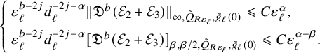 $$ \begin{align} \left\{ \begin{array}{ll} \varepsilon_{\ell}^{b-2j} d_{\ell}^{-2j-{\alpha}} \|\mathfrak{D}^b(\mathcal{E}_2+\mathcal{E}_3)\|_{\infty, \tilde Q_{R\varepsilon_{\ell}},\tilde g_{\ell}(0)}\leqslant C\varepsilon_{\ell}^{\alpha},\\[2mm] \varepsilon_{\ell}^{b-2j} d_{\ell}^{-2j-{\alpha}} [ \mathfrak{D}^b (\mathcal{E}_2+\mathcal{E}_3)]_{{\beta},{\beta}/2, \tilde Q_{R\varepsilon_{\ell}},\tilde g_{\ell}(0)}\leqslant C\varepsilon_{\ell}^{{\alpha}-{\beta}}. \end{array} \right. \end{align} $$
Observe that (4.301) for
 $a\leqslant 2j$
and
$a\leqslant 2j$
and
 ${\beta }={\alpha }$
is exactly given by (4.222) and (4.223). To prove it for
${\beta }={\alpha }$
is exactly given by (4.222) and (4.223). To prove it for
 $a\geqslant 2j$
and
$a\geqslant 2j$
and
 ${\beta }\geqslant \alpha $
, we apply the diffeomorphism
${\beta }\geqslant \alpha $
, we apply the diffeomorphism
 $\Pi _{\ell }$
in (4.285) so that
$\Pi _{\ell }$
in (4.285) so that
 $\Pi _{\ell }^{*}(\mathcal {E}_2+\mathcal {E}_3)$
equals
$\Pi _{\ell }^{*}(\mathcal {E}_2+\mathcal {E}_3)$
equals
 $$ \begin{align} \log \frac{(\check\omega_{\ell}^\sharp)^{m+n}}{ \binom{m+n}{m}\check\omega_{\ell,\mathrm{can}} ^m \wedge (\Sigma_{\ell}^{*} \omega_F)^n}+ne^{-t_{\ell}}\check t -\sum_{i=1}^j\sum_{p=1}^{N_{i,k}} \check{\mathfrak{G}}_{\check{t},k}\left(\partial_{\check{t}}\check A_{\ell,i,p,k}^\sharp +e^{-t_{\ell}}\check A_{\ell,i,p,k}^\sharp,\check G_{\ell,i,p,k} \right)-e^{-e^{-t_{\ell}}\check t}\partial_{\check t}\underline{\check\chi_{\ell}^\sharp}, \end{align} $$
and for any
 $b\geqslant 0$
, we have
$b\geqslant 0$
, we have
 $$ \begin{align} \varepsilon_{\ell}^{-\alpha}\varepsilon_{\ell}^{b-2j}d_{\ell}^{-2j-\alpha}\|\mathfrak{D}^b(\mathcal{E}_2+\mathcal{E}_3)\|_{\infty, \tilde Q_{R\varepsilon_{\ell}},\tilde g_{\ell}(0)} =\delta_{\ell}^{-2j-\alpha}\|\mathfrak{D}^b(\Pi_{\ell}^{*}(\mathcal{E}_2+\mathcal{E}_3))\|_{\infty, \check Q_{R},\check g_{\ell}(0)}, \end{align} $$
 $$ \begin{align} \varepsilon_{\ell}^{\beta-\alpha}\varepsilon_{\ell}^{b-2j}d_{\ell}^{-2j-\alpha}[\mathfrak{D}^b(\mathcal{E}_2+\mathcal{E}_3)]_{\beta,\beta/2, \tilde Q_{R\varepsilon_{\ell}},\tilde g_{\ell}(0)} =\delta_{\ell}^{-2j-\alpha}[\mathfrak{D}^b(\Pi_{\ell}^{*}(\mathcal{E}_2+\mathcal{E}_3))]_{\beta,\beta/2, \check Q_{R},\check g_{\ell}(0)}. \end{align} $$
So thanks to (4.301), we see that
 $\delta _{\ell }^{-2j-\alpha }\Pi _{\ell }^{*}(\mathcal {E}_2+\mathcal {E}_3)$
is locally uniformly bounded in
$\delta _{\ell }^{-2j-\alpha }\Pi _{\ell }^{*}(\mathcal {E}_2+\mathcal {E}_3)$
is locally uniformly bounded in
 $C^{2j+\alpha ,j+{\alpha }/2}$
with respect to the (essentially fixed) metric
$C^{2j+\alpha ,j+{\alpha }/2}$
with respect to the (essentially fixed) metric
 $\check {g}_{\ell }(0)$
, so by Ascoli-Arzelà, up to passing to a subsequence, it converges locally uniformly on
$\check {g}_{\ell }(0)$
, so by Ascoli-Arzelà, up to passing to a subsequence, it converges locally uniformly on
 $\mathbb {C}^m\times Y\times (-\infty ,0]$
to some limiting function
$\mathbb {C}^m\times Y\times (-\infty ,0]$
to some limiting function
 $\mathcal {F}$
. Since the quantity
$\mathcal {F}$
. Since the quantity
 $-\delta _{\ell }^{-2j-\alpha }\Pi _{\ell }^{*}(\mathcal {E}_2+\mathcal {E}_3)$
is exactly (3.15), we would like to apply the Selection Theorem 3.1, so we check that its hypotheses are satisfied. The functions
$-\delta _{\ell }^{-2j-\alpha }\Pi _{\ell }^{*}(\mathcal {E}_2+\mathcal {E}_3)$
is exactly (3.15), we would like to apply the Selection Theorem 3.1, so we check that its hypotheses are satisfied. The functions
 $\hat {A}_{\ell ,i,p,k}$
satisfy (3.7) with
$\hat {A}_{\ell ,i,p,k}$
satisfy (3.7) with
 $\alpha _0=\frac {\alpha ^2}{2j+\alpha }$
thanks to (4.172), while the function
$\alpha _0=\frac {\alpha ^2}{2j+\alpha }$
thanks to (4.172), while the function
 $-e^{-\lambda _{\ell }^{-2}\hat t}\partial _{\hat t}\underline{\hat \chi _{\ell }^\sharp }-n\lambda _{\ell }^{-2}\hat {t}$
converges to
$-e^{-\lambda _{\ell }^{-2}\hat t}\partial _{\hat t}\underline{\hat \chi _{\ell }^\sharp }-n\lambda _{\ell }^{-2}\hat {t}$
converges to
 $0$
locally smoothly thanks to (4.158). We can thus apply the Selection Theorem and conclude that
$0$
locally smoothly thanks to (4.158). We can thus apply the Selection Theorem and conclude that
 $\delta _{\ell }^{-2j-\alpha }\Pi _{\ell }^{*}(\mathcal {E}_2+\mathcal {E}_3)$
converges to
$\delta _{\ell }^{-2j-\alpha }\Pi _{\ell }^{*}(\mathcal {E}_2+\mathcal {E}_3)$
converges to
 $\mathcal {F}$
locally smoothly, and hence, its derivatives of all orders are uniformly bounded on
$\mathcal {F}$
locally smoothly, and hence, its derivatives of all orders are uniformly bounded on
 $\check Q_{R}$
. Thanks to (4.303), (4.304), this proves that (4.301) holds for all
$\check Q_{R}$
. Thanks to (4.303), (4.304), this proves that (4.301) holds for all
 $b\geqslant 0$
and
$b\geqslant 0$
and
 ${\alpha }\leqslant \beta <1$
. Recalling then that
${\alpha }\leqslant \beta <1$
. Recalling then that
 ${i\partial \bar \partial } =\tilde J_{\ell }\circledast {\mathbb {D}}^2+{\mathbb {D}} \tilde J_{\ell }\circledast {\mathbb {D}}$
, and using the bounds in (4.176) for
${i\partial \bar \partial } =\tilde J_{\ell }\circledast {\mathbb {D}}^2+{\mathbb {D}} \tilde J_{\ell }\circledast {\mathbb {D}}$
, and using the bounds in (4.176) for
 $\tilde {J}_{\ell }$
and its derivatives, these imply directly that for all
$\tilde {J}_{\ell }$
and its derivatives, these imply directly that for all
 $a\geqslant 2, {\alpha }\leqslant \beta <1,$
 $$ \begin{align} C\varepsilon_{\ell}^{a-2j}d_{\ell}^{-2j-{\alpha}}\left[\mathfrak{D}^{a-2}{i\partial\bar\partial}(\mathcal{E}_2+\mathcal{E}_3)\right]_{{\beta},{\beta}/2,\tilde Q_{R\varepsilon_{\ell}},\tilde g_{\ell}(0)}\leqslant C\varepsilon_{\ell}^{\alpha-\beta}. \end{align} $$
Next, we consider the term
 $\mathcal {E}_1$
. Recall that
$\mathcal {E}_1$
. Recall that
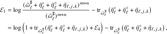 $$ \begin{align} \begin{aligned} \mathcal{E}_1&= \log \frac{(\tilde \omega_{\ell}^\sharp +\tilde{\eta}_{\ell}^\circ+\tilde{\eta}_{\ell}^\diamondsuit+\tilde{\eta}_{\ell,j,k})^{m+n}}{ (\tilde{\omega}_{\ell}^\sharp)^{m+n}}-\operatorname{tr}_{\tilde \omega_{\ell}^\sharp}\left(\tilde{\eta}_{\ell}^\circ+\tilde{\eta}_{\ell}^\diamondsuit+\tilde{\eta}_{\ell,j,k}\right)\\ &=\log \left(1+\operatorname{tr}_{\tilde \omega_{\ell}^\sharp}(\tilde{\eta}_{\ell}^\circ+\tilde{\eta}_{\ell}^\diamondsuit+\tilde{\eta}_{\ell,j,k})+\mathcal{E}_4 \right)-\operatorname{tr}_{\tilde \omega_{\ell}^\sharp}\left(\tilde{\eta}_{\ell}^\circ+\tilde{\eta}_{\ell}^\diamondsuit+\tilde{\eta}_{\ell,j,k}\right), \end{aligned} \end{align} $$
where
 $\mathcal {E}_4$
was defined in (4.227). Taking
$\mathcal {E}_4$
was defined in (4.227). Taking
 $\mathfrak {D}^{a}$
derivatives, for
$\mathfrak {D}^{a}$
derivatives, for
 $a\geqslant 2j\geqslant 2,a\in 2\mathbb {N}$
, we again expand it schematically as in (4.229). The first step is to prove estimates for
$a\geqslant 2j\geqslant 2,a\in 2\mathbb {N}$
, we again expand it schematically as in (4.229). The first step is to prove estimates for
 $\mathcal {E}_4$
, and for this, we observe that
$\mathcal {E}_4$
, and for this, we observe that
 $\varepsilon _{\ell }^{a-2j}d_{\ell }^{-2j-{\alpha }}\mathcal {E}_4$
is identical to the term
$\varepsilon _{\ell }^{a-2j}d_{\ell }^{-2j-{\alpha }}\mathcal {E}_4$
is identical to the term
 $\mathcal {N}$
in [Reference Hein and Tosatti21, (4.268)], and we will bound it following the discussion there. To do this, we need some basic estimates first. Using (4.209), we have for all
$\mathcal {N}$
in [Reference Hein and Tosatti21, (4.268)], and we will bound it following the discussion there. To do this, we need some basic estimates first. Using (4.209), we have for all
 $\iota \geqslant 0$
that
$\iota \geqslant 0$
that
 $$ \begin{align} [\mathfrak{D}^\iota \tilde{\omega}_{\ell}^\sharp]_{{\beta},{\beta}/2,\tilde Q_{O(\varepsilon_{\ell})},\tilde g_{\ell}(0)}\leqslant C\varepsilon_{\ell}^{-{\beta}-\iota},\;\;\; \|\mathfrak{D}^\iota \tilde{\omega}_{\ell}^\sharp\|_{\infty,\tilde Q_{O(\varepsilon_{\ell})},\tilde g_{\ell}(0)}\leqslant C\varepsilon_{\ell}^{-\iota}. \end{align} $$
Next, we observe that for all
 ${\alpha }\leqslant {\beta }<1$
and
${\alpha }\leqslant {\beta }<1$
and
 $0\leqslant \iota <\max (a-1,2j)$
, we have
$0\leqslant \iota <\max (a-1,2j)$
, we have
 $$ \begin{align} \|\mathfrak{D}^\iota(\tilde{\eta}_{\ell}^\circ+\tilde{\eta}_{\ell}^\diamondsuit+\tilde{\eta}_{\ell,j,k})\|_{\infty,\tilde Q_{O(\varepsilon_{\ell})},\tilde g_{\ell}(0)}\leqslant C\delta_{\ell}^{2j+{\alpha}}\varepsilon_{\ell}^{-\iota}, \quad [\mathfrak{D}^\iota (\tilde{\eta}_{\ell}^\circ+\tilde{\eta}_{\ell}^\diamondsuit+\tilde{\eta}_{\ell,j,k})]_{{\beta},{\beta}/2,\tilde Q_{O(\varepsilon_{\ell})},\tilde g_{\ell}(0)}\leqslant C\delta_{\ell}^{2j+{\alpha}}\varepsilon_{\ell}^{-\iota-{\beta}}. \end{align} $$
Indeed, these estimates are already known to hold for
 $\iota \leqslant 2j$
and
$\iota \leqslant 2j$
and
 $\beta ={\alpha }$
thanks to (4.145), (4.153) and (4.181); hence, using interpolation, they also hold for
$\beta ={\alpha }$
thanks to (4.145), (4.153) and (4.181); hence, using interpolation, they also hold for
 $\iota <2j$
and
$\iota <2j$
and
 $\alpha \leqslant \beta <1$
, while if
$\alpha \leqslant \beta <1$
, while if
 $\iota <a-1, {\alpha }\leqslant {\beta }<1$
, these also hold thanks to the estimates (4.295) which hold by the induction hypothesis. Recalling that in this section we have
$\iota <a-1, {\alpha }\leqslant {\beta }<1$
, these also hold thanks to the estimates (4.295) which hold by the induction hypothesis. Recalling that in this section we have
 $j\geqslant 1$
, it follows that
$j\geqslant 1$
, it follows that
 $\max (a-1,2j)\geqslant 2$
.
$\max (a-1,2j)\geqslant 2$
.
From (4.308) and the definition of
 $\mathcal {E}_4$
in (4.227), it follows immediately that for
$\mathcal {E}_4$
in (4.227), it follows immediately that for
 $0\leqslant \iota <\max (a-1,2j)$
and
$0\leqslant \iota <\max (a-1,2j)$
and
 ${\alpha }\leqslant {\beta }<1$
, we have
${\alpha }\leqslant {\beta }<1$
, we have
 $$ \begin{align} \varepsilon_{\ell}^{a-2j}d_{\ell}^{-2j-\alpha}\|\mathfrak{D}^\iota\mathcal{E}_4\|_{\infty,\tilde Q_{O(\varepsilon_{\ell})},\tilde g_{\ell}(0)}\leqslant C\varepsilon_{\ell}^{a+\alpha-\iota} \delta_{\ell}^{2j+\alpha}, \quad\varepsilon_{\ell}^{a-2j}d_{\ell}^{-2j-\alpha}[\mathfrak{D}^\iota\mathcal{E}_4]_{{\beta},{\beta}/2,\tilde Q_{O(\varepsilon_{\ell})},\tilde g_{\ell}(0)}\leqslant C\varepsilon_{\ell}^{a+\alpha-\iota-\beta}\delta_{\ell}^{2j+\alpha}. \end{align} $$
However, we do not have the estimates (4.308) when
 $a-1\leqslant \iota \leqslant a$
and
$a-1\leqslant \iota \leqslant a$
and
 $\iota \geqslant 2j$
, since our induction argument is only on even values of
$\iota \geqslant 2j$
, since our induction argument is only on even values of
 $a\geqslant 2j$
, and this is different from the discussion in [Reference Hein and Tosatti21, §4.10.3]. To accommodate for the missing term with derivatives of order between
$a\geqslant 2j$
, and this is different from the discussion in [Reference Hein and Tosatti21, §4.10.3]. To accommodate for the missing term with derivatives of order between
 $a-1$
and a, we apply Proposition 2.3 with (4.308) so that
$a-1$
and a, we apply Proposition 2.3 with (4.308) so that
 $$ \begin{align} \|\mathfrak{D}^{a-1}(\tilde{\eta}_{\ell}^\circ+\tilde{\eta}_{\ell}^\diamondsuit+\tilde{\eta}_{\ell,j,k})\|_{\infty,\tilde Q_{\tilde R},\tilde g_{\ell}(0)}\leqslant C\varepsilon_{\ell}^{1+{\beta}}[\mathfrak{D}^{a}(\tilde{\eta}_{\ell}^\circ+\tilde{\eta}_{\ell}^\diamondsuit+\tilde{\eta}_{\ell,j,k})]_{{\beta},{\beta}/2,\tilde Q_{R},\tilde g_{\ell}(0)}+C\delta_{\ell}^{2j+{\alpha}} (R-\rho)^{-1}\varepsilon_{\ell}^{-a+2}, \end{align} $$
 $$ \begin{align} \begin{aligned} [\mathfrak{D}^{a-1}(\tilde{\eta}_{\ell}^\circ+\tilde{\eta}_{\ell}^\diamondsuit+\tilde{\eta}_{\ell,j,k})]_{{\beta},{\beta}/2,\tilde Q_{\tilde R},\tilde g_{\ell}(0)}&\leqslant C\varepsilon_{\ell} [\mathfrak{D}^{a}(\tilde{\eta}_{\ell}^\circ+\tilde{\eta}_{\ell}^\diamondsuit+\tilde{\eta}_{\ell,j,k})]_{{\beta},{\beta}/2,\tilde Q_{R},\tilde g_{\ell}(0)}+C\delta_{\ell}^{2j+{\alpha}} (R-\rho)^{-{\beta}-1} \varepsilon_{\ell}^{-a+2}, \end{aligned} \end{align} $$
 $$ \begin{align} \|\mathfrak{D}^{a}(\tilde{\eta}_{\ell}^\circ+\tilde{\eta}_{\ell}^\diamondsuit+\tilde{\eta}_{\ell,j,k})\|_{\infty,\tilde Q_{\tilde R},\tilde g_{\ell}(0)}\leqslant C\varepsilon_{\ell}^{{\beta}}[\mathfrak{D}^{a}(\tilde{\eta}_{\ell}^\circ+\tilde{\eta}_{\ell}^\diamondsuit+\tilde{\eta}_{\ell,j,k})]_{{\beta},{\beta}/2,\tilde Q_{R},\tilde g_{\ell}(0)}+C\delta_{\ell}^{2j+{\alpha}} (R-\rho)^{-2}\varepsilon_{\ell}^{-a+2}. \end{align} $$
Given these, we can use the same method as in [Reference Hein and Tosatti21, (4.272)–(4.275)] and see that for every
 $\iota $
with
$\iota $
with
 $\max (a-1,2j)\leqslant \iota \leqslant a$
and
$\max (a-1,2j)\leqslant \iota \leqslant a$
and
 $\alpha \leqslant \beta <1$
, we have
$\alpha \leqslant \beta <1$
, we have
 $$ \begin{align} \varepsilon_{\ell}^{a-2j}d_{\ell}^{-2j-\alpha}\|\mathfrak{D}^\iota\mathcal{E}_4\|_{\infty,\tilde Q_{\tilde R},\tilde g_{\ell}(0)}&\leqslant o(1)\varepsilon_{\ell}^{a+\beta-\iota}\varepsilon_{\ell}^{a-2j}d_{\ell}^{-2j-\alpha}[\mathfrak{D}^a (\tilde{\eta}_{\ell}^\circ+\tilde{\eta}_{\ell}^\diamondsuit+\tilde{\eta}_{\ell,j,k})]_{{\beta},{\beta}/2,\tilde Q_R,\tilde g_{\ell}(0)}\nonumber\\& \quad +C(R-\rho)^{-\iota}\delta_{\ell}^{2j+\alpha}\varepsilon_{\ell}^{a+\alpha}, \end{align} $$
and for
 $\max (a-1,2j)\leqslant \iota <a, \alpha \leqslant \beta <1$
,
$\max (a-1,2j)\leqslant \iota <a, \alpha \leqslant \beta <1$
,
 $$ \begin{align} \varepsilon_{\ell}^{a-2j}d_{\ell}^{-2j-\alpha}[\mathfrak{D}^\iota\mathcal{E}_4]_{{\beta},{\beta}/2,\tilde Q_{\tilde R},\tilde g_{\ell}(0)}&\leqslant o(1)\varepsilon_{\ell}^{a-\iota}\varepsilon_{\ell}^{a-2j}d_{\ell}^{-2j-\alpha}[\mathfrak{D}^a (\tilde{\eta}_{\ell}^\circ+\tilde{\eta}_{\ell}^\diamondsuit+\tilde{\eta}_{\ell,j,k})]_{{\beta},{\beta}/2,\tilde Q_R,\tilde g_{\ell}(0)}\nonumber\\& \quad +C(R-\rho)^{-\iota-\beta}\delta_{\ell}^{2j+\alpha}\varepsilon_{\ell}^{a+\alpha}, \end{align} $$
while for
 $\iota =a$
,
$\iota =a$
,
 $$ \begin{align} \varepsilon_{\ell}^{a-2j}d_{\ell}^{-2j-\alpha}[\mathfrak{D}^a\mathcal{E}_4]_{{\beta},{\beta}/2,\tilde Q_{\tilde R},\tilde g_{\ell}(0)}\leqslant o(1)\varepsilon_{\ell}^{a-2j}d_{\ell}^{-2j-\alpha}[\mathfrak{D}^a (\tilde{\eta}_{\ell}^\circ+\tilde{\eta}_{\ell}^\diamondsuit+\tilde{\eta}_{\ell,j,k})]_{{\beta},{\beta}/2,\tilde Q_R,\tilde g_{\ell}(0)}. \end{align} $$
One important observation that we used here is that whenever we need to use (4.310), (4.311) or (4.312) for some term in
 $\mathcal {E}_4$
, the remaining part of this summand in
$\mathcal {E}_4$
, the remaining part of this summand in
 $\mathcal {E}_4$
is hit by at most
$\mathcal {E}_4$
is hit by at most
 $1+\beta $
derivatives, and since
$1+\beta $
derivatives, and since
 $1+\beta <2\leqslant \max (a-1,2j)$
, for these other terms, we are allowed to apply (4.308).
$1+\beta <2\leqslant \max (a-1,2j)$
, for these other terms, we are allowed to apply (4.308).
Now that we have our estimates for
 $\mathcal {E}_4$
, we need estimates on derivatives of
$\mathcal {E}_4$
, we need estimates on derivatives of
 $\operatorname {tr}_{\tilde {\omega }_{\ell }^\sharp }(\tilde {\eta }_{\ell }^\circ +\tilde {\eta }_{\ell }^\diamondsuit +\tilde {\eta }_{\ell ,j,k})$
. For this, from (4.307) and (4.308), we see that for
$\operatorname {tr}_{\tilde {\omega }_{\ell }^\sharp }(\tilde {\eta }_{\ell }^\circ +\tilde {\eta }_{\ell }^\diamondsuit +\tilde {\eta }_{\ell ,j,k})$
. For this, from (4.307) and (4.308), we see that for
 $0\leqslant \iota <\max (a-1,2j), {\alpha }\leqslant {\beta }<1$
,
$0\leqslant \iota <\max (a-1,2j), {\alpha }\leqslant {\beta }<1$
,
 $$ \begin{align} \varepsilon_{\ell}^{a-2j}d_{\ell}^{-2j-\alpha}\|\mathfrak{D}^\iota\operatorname{tr}_{\tilde{\omega}_{\ell}^\sharp}(\tilde{\eta}_{\ell}^\circ+\tilde{\eta}_{\ell}^\diamondsuit+\tilde{\eta}_{\ell,j,k})\|_{\infty,\tilde Q_{\tilde R},\tilde g_{\ell}(0)}\leqslant C\varepsilon_{\ell}^{a+\alpha-\iota}, \end{align} $$
 $$ \begin{align} \varepsilon_{\ell}^{a-2j}d_{\ell}^{-2j-\alpha}[\mathfrak{D}^\iota\operatorname{tr}_{\tilde{\omega}_{\ell}^\sharp}(\tilde{\eta}_{\ell}^\circ+\tilde{\eta}_{\ell}^\diamondsuit+\tilde{\eta}_{\ell,j,k})]_{{\beta},{\beta}/2,\tilde Q_{\tilde R},\tilde g_{\ell}(0)}\leqslant C\varepsilon_{\ell}^{a+\alpha-\iota-\beta}, \end{align} $$
while for derivatives of order
 $a-1\leqslant \iota \leqslant a$
and
$a-1\leqslant \iota \leqslant a$
and
 $\iota \geqslant 2j$
, we can argue as above and estimate crudely
$\iota \geqslant 2j$
, we can argue as above and estimate crudely
 $$ \begin{align} \varepsilon_{\ell}^{a-2j}d_{\ell}^{-2j-\alpha}\|\mathfrak{D}^\iota\operatorname{tr}_{\tilde{\omega}_{\ell}^\sharp}(\tilde{\eta}_{\ell}^\circ+\tilde{\eta}_{\ell}^\diamondsuit+\tilde{\eta}_{\ell,j,k})\|_{\infty,\tilde Q_{\tilde R},\tilde g_{\ell}(0)}&\leqslant C\varepsilon_{\ell}^{a+\beta-\iota}\varepsilon_{\ell}^{a-2j}d_{\ell}^{-2j-\alpha}[\mathfrak{D}^a (\tilde{\eta}_{\ell}^\circ+\tilde{\eta}_{\ell}^\diamondsuit+\tilde{\eta}_{\ell,j,k})]_{{\beta},{\beta}/2,\tilde Q_R,\tilde g_{\ell}(0)}\nonumber\\&\quad+C(R-\rho)^{-\iota}\varepsilon_{\ell}^{a+\alpha}, \end{align} $$
 $$ \begin{align} \varepsilon_{\ell}^{a-2j}d_{\ell}^{-2j-\alpha}[\mathfrak{D}^\iota\operatorname{tr}_{\tilde{\omega}_{\ell}^\sharp}(\tilde{\eta}_{\ell}^\circ+\tilde{\eta}_{\ell}^\diamondsuit+\tilde{\eta}_{\ell,j,k})]_{{\beta},{\beta}/2,\tilde Q_{\tilde R},\tilde g_{\ell}(0)}&\leqslant C\varepsilon_{\ell}^{a-\iota}\varepsilon_{\ell}^{a-2j}d_{\ell}^{-2j-\alpha}[\mathfrak{D}^a (\tilde{\eta}_{\ell}^\circ+\tilde{\eta}_{\ell}^\diamondsuit+\tilde{\eta}_{\ell,j,k})]_{{\beta},{\beta}/2,\tilde Q_R,\tilde g_{\ell}(0)}\nonumber\\&\quad+C(R-\rho)^{-\iota-\beta}\varepsilon_{\ell}^{a+\alpha}. \end{align} $$
Equipped with (4.309), (4.313), (4.314), (4.315), (4.316), (4.317), (4.318) and (4.319), we proceed to estimate derivatives of
 $\mathcal {E}_1$
. We first consider the first line of (4.229), which we can write as
$\mathcal {E}_1$
. We first consider the first line of (4.229), which we can write as
 $$ \begin{align} -\mathfrak{D}^a \operatorname{tr}_{\tilde{\omega}_{\ell}^\sharp}(\tilde{\eta}_{\ell}^\circ+\tilde{\eta}_{\ell}^\diamondsuit+\tilde{\eta}_{\ell,j,k}) \frac{\operatorname{tr}_{\tilde{\omega}_{\ell}^\sharp}(\tilde{\eta}_{\ell}^\circ+\tilde{\eta}_{\ell}^\diamondsuit+\tilde{\eta}_{\ell,j,k})+\mathcal{E}_4}{1+\operatorname{tr}_{\tilde{\omega}_{\ell}^\sharp}(\tilde{\eta}_{\ell}^\circ+\tilde{\eta}_{\ell}^\diamondsuit+\tilde{\eta}_{\ell,j,k})+\mathcal{E}_4} +\frac{\mathfrak{D}^a \mathcal{E}_4}{1+\operatorname{tr}_{\tilde{\omega}_{\ell}^\sharp}(\tilde{\eta}_{\ell}^\circ+\tilde{\eta}_{\ell}^\diamondsuit+\tilde{\eta}_{\ell,j,k})+\mathcal{E}_4}, \end{align} $$
and we take
 $\varepsilon _{\ell }^{a-2j}d_{\ell }^{-2j-\alpha }[\cdot ]_{{\beta },{\beta }/2,\tilde Q_{\tilde R},\tilde g_{\ell }(0)}$
of this. Since
$\varepsilon _{\ell }^{a-2j}d_{\ell }^{-2j-\alpha }[\cdot ]_{{\beta },{\beta }/2,\tilde Q_{\tilde R},\tilde g_{\ell }(0)}$
of this. Since
 $|\operatorname {tr}_{\tilde {\omega }_{\ell }^\sharp }(\tilde {\eta }_{\ell }^\circ +\tilde {\eta }_{\ell }^\diamondsuit +\tilde {\eta }_{\ell ,j,k})+\mathcal {E}_4|=o(1)$
, when the difference quotient lands on
$|\operatorname {tr}_{\tilde {\omega }_{\ell }^\sharp }(\tilde {\eta }_{\ell }^\circ +\tilde {\eta }_{\ell }^\diamondsuit +\tilde {\eta }_{\ell ,j,k})+\mathcal {E}_4|=o(1)$
, when the difference quotient lands on
 $\mathfrak {D}^a \mathrm {tr}$
, we can estimate this by
$\mathfrak {D}^a \mathrm {tr}$
, we can estimate this by
 $o(1)$
times (4.319) (with
$o(1)$
times (4.319) (with
 $\iota =a$
). Similarly,
$\iota =a$
). Similarly,
 $[\operatorname {tr}_{\tilde {\omega }_{\ell }^\sharp }(\tilde {\eta }_{\ell }^\circ +\tilde {\eta }_{\ell }^\diamondsuit +\tilde {\eta }_{\ell ,j,k})+\mathcal {E}_4]_{C^\beta }=o(\varepsilon _{\ell }^{-\beta })$
, so when the difference quotient lands on
$[\operatorname {tr}_{\tilde {\omega }_{\ell }^\sharp }(\tilde {\eta }_{\ell }^\circ +\tilde {\eta }_{\ell }^\diamondsuit +\tilde {\eta }_{\ell ,j,k})+\mathcal {E}_4]_{C^\beta }=o(\varepsilon _{\ell }^{-\beta })$
, so when the difference quotient lands on
 $\frac {\mathrm {tr}+\mathcal {E}_4}{1+\mathrm {tr}+\mathcal {E}_4}$
, we can estimate this by
$\frac {\mathrm {tr}+\mathcal {E}_4}{1+\mathrm {tr}+\mathcal {E}_4}$
, we can estimate this by
 $o(\varepsilon _{\ell }^{-\beta })$
times (4.318) (with
$o(\varepsilon _{\ell }^{-\beta })$
times (4.318) (with
 $\iota =a$
). And when the difference quotient lands on
$\iota =a$
). And when the difference quotient lands on
 $\frac {\mathfrak {D}^a\mathcal {E}_4}{1+\mathrm {tr}+\mathcal {E}_4}$
, we argue similarly with (4.313) and (4.315). So all together when we apply
$\frac {\mathfrak {D}^a\mathcal {E}_4}{1+\mathrm {tr}+\mathcal {E}_4}$
, we argue similarly with (4.313) and (4.315). So all together when we apply
 $\varepsilon _{\ell }^{a-2j}d_{\ell }^{-2j-\alpha }[\cdot ]_{{\beta },{\beta }/2,\tilde Q_{\tilde R},\tilde g_{\ell }(0)}$
to (4.320), we can bound it by
$\varepsilon _{\ell }^{a-2j}d_{\ell }^{-2j-\alpha }[\cdot ]_{{\beta },{\beta }/2,\tilde Q_{\tilde R},\tilde g_{\ell }(0)}$
to (4.320), we can bound it by
 $$ \begin{align} o(1)\varepsilon_{\ell}^{a-2j}d_{\ell}^{-2j-\alpha}[\mathfrak{D}^a (\tilde{\eta}_{\ell}^\circ+\tilde{\eta}_{\ell}^\diamondsuit+\tilde{\eta}_{\ell,j,k})]_{{\beta},{\beta}/2,\tilde Q_R,\tilde g_{\ell}(0)}+ C(R-\rho)^{-a-\beta}\varepsilon_{\ell}^{a+\alpha}+C(R-\rho)^{-a}\varepsilon_{\ell}^{a+\alpha-\beta}. \end{align} $$
Lastly, we need to consider what happens when we take
 $\varepsilon _{\ell }^{a-2j}d_{\ell }^{-2j-\alpha }[\cdot ]_{{\beta },{\beta }/2,\tilde Q_{\tilde R},\tilde g_{\ell }(0)}$
of the large sum in the second line of (4.229). If all the derivatives that appear there are of order
$\varepsilon _{\ell }^{a-2j}d_{\ell }^{-2j-\alpha }[\cdot ]_{{\beta },{\beta }/2,\tilde Q_{\tilde R},\tilde g_{\ell }(0)}$
of the large sum in the second line of (4.229). If all the derivatives that appear there are of order
 $<\max (a-1,2j)$
, then this is bounded by
$<\max (a-1,2j)$
, then this is bounded by
 $o(\varepsilon _{\ell }^{\alpha -\beta })$
, while if there is at least one derivative of order at least
$o(\varepsilon _{\ell }^{\alpha -\beta })$
, while if there is at least one derivative of order at least
 $\max (a-1,2j)$
(to which we apply (4.313)–(4.315), (4.318)–(4.319)), then all other derivatives in total are of order at most
$\max (a-1,2j)$
(to which we apply (4.313)–(4.315), (4.318)–(4.319)), then all other derivatives in total are of order at most
 $1$
(and to these we can instead apply (4.309), (4.316)–(4.317)). Putting all these together proves that
$1$
(and to these we can instead apply (4.309), (4.316)–(4.317)). Putting all these together proves that
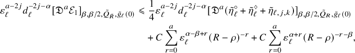 $$ \begin{align} \begin{aligned} \varepsilon_{\ell}^{a-2j}d_{\ell}^{-2j-{\alpha}} [\mathfrak{D}^a\mathcal{E}_1]_{{\beta},{\beta}/2,\tilde Q_{\tilde R},\tilde g_{\ell}(0)}&\leqslant \frac{1}{4}\varepsilon_{\ell}^{a-2j} d_{\ell}^{-2j-{\alpha}} [\mathfrak{D}^a (\tilde{\eta}_{\ell}^\circ+\tilde{\eta}_{\ell}^\diamondsuit+\tilde{\eta}_{\ell,j,k})]_{{\beta},{\beta}/2,\tilde Q_R,\tilde g_{\ell}(0)}\\ &\quad +C\sum_{r=0}^a \varepsilon_{\ell}^{{\alpha}-{\beta}+r}(R-\rho)^{-r}+C\sum_{r=0}^{a}\varepsilon_{\ell}^{{\alpha}+r} (R-\rho)^{-r-\beta}, \end{aligned} \end{align} $$
and combining this with (4.305) completes the proof of Claim 4.9.
For later use, observe also that the same argument gives an analogous bound for the
 $L^\infty $
norm of derivatives of
$L^\infty $
norm of derivatives of
 $\mathcal {E}_1$
– namely,
$\mathcal {E}_1$
– namely,
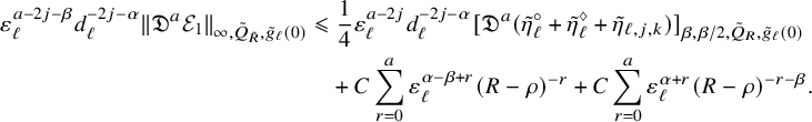 $$ \begin{align} \begin{aligned} \varepsilon_{\ell}^{a-2j-{\beta}}d_{\ell}^{-2j-{\alpha}} \|\mathfrak{D}^a\mathcal{E}_1\|_{\infty,\tilde Q_{\tilde R},\tilde g_{\ell}(0)}&\leqslant \frac{1}{4}\varepsilon_{\ell}^{a-2j} d_{\ell}^{-2j-{\alpha}} [\mathfrak{D}^a (\tilde{\eta}_{\ell}^\circ+\tilde{\eta}_{\ell}^\diamondsuit+\tilde{\eta}_{\ell,j,k})]_{{\beta},{\beta}/2,\tilde Q_R,\tilde g_{\ell}(0)}\\ &\quad +C\sum_{r=0}^a \varepsilon_{\ell}^{{\alpha}-{\beta}+r}(R-\rho)^{-r}+C\sum_{r=0}^{a}\varepsilon_{\ell}^{{\alpha}+r} (R-\rho)^{-r-\beta}. \end{aligned} \end{align} $$
4.12.4 Killing the contributions from
$\underline{\tilde {\chi }^{*}_{\ell }}$

The starting point is (4.232) with
 $a=2j$
and radius
$a=2j$
and radius
 $C\delta _{\ell }$
. For
$C\delta _{\ell }$
. For
 $0\leqslant b\leqslant 2j$
, we first bound the term
$0\leqslant b\leqslant 2j$
, we first bound the term
 $$ \begin{align} \|\mathfrak{D}^b{i\partial\bar\partial} \hat\varphi_{\ell}\|_{\infty,\hat Q_{C\delta_{\ell}},g_X}\leqslant C\|\mathfrak{D}^b(\hat{\eta}^\diamondsuit_{\ell}+\hat{\eta}^\ddagger_{\ell}+\hat{\eta}^\circ_{\ell}+\hat{\eta}_{\ell,j,k})\|_{\infty,\hat Q_{C\delta_{\ell}},\hat{g}_{\ell}(0)}+\|\mathfrak{D}^b\hat{\eta}^\dagger_{\ell}\|_{\infty,\hat Q_{C\delta_{\ell}},g_X}\leqslant C, \end{align} $$
using (4.145), (4.159), (4.160), (4.189), (4.190) and (4.202). Using this, we transfer (4.232) to the tilde picture and multiply it by
 $d_{\ell }^{\beta -\alpha }$
and get
$d_{\ell }^{\beta -\alpha }$
and get
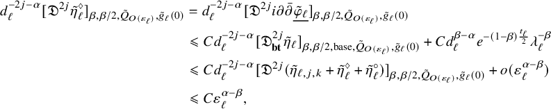 $$ \begin{align} \begin{aligned} d_{\ell}^{-2j-\alpha}[\mathfrak{D}^{2j}\tilde{\eta}^\diamondsuit_{\ell}]_{{\beta},{\beta}/2,\tilde{Q}_{O(\varepsilon_{\ell})},\tilde g_{\ell}(0)}&= d_{\ell}^{-2j-\alpha}[\mathfrak{D}^{2j}{i\partial\bar\partial}\underline{\tilde{\varphi}_{\ell}}]_{{\beta},{\beta}/2,\tilde{Q}_{O(\varepsilon_{\ell})},\tilde g_{\ell}(0)}\\ &\leqslant Cd_{\ell}^{-2j-\alpha}[\mathfrak{D}^{2j}_{\mathbf{bt}}\tilde{\eta}_{\ell}]_{{\beta},{\beta}/2,\textrm{base},\tilde{Q}_{O(\varepsilon_{\ell})},\tilde g_{\ell}(0)}+Cd_{\ell}^{{\beta}-{\alpha}}e^{-(1-\beta)\frac{t_{\ell}}{2}}\lambda_{\ell}^{-\beta}\\ &\leqslant Cd_{\ell}^{-2j-\alpha}[\mathfrak{D}^{2j} (\tilde \eta_{\ell,j,k}+\tilde \eta_{\ell}^\diamondsuit+\tilde{\eta}_{\ell}^\circ)]_{{\beta},{\beta}/2,\tilde Q_{O(\varepsilon_{\ell})},\tilde g_{\ell}(0)}+o(\varepsilon_{\ell}^{{\alpha}-{\beta}})\\ &\leqslant C\varepsilon_{\ell}^{{\alpha}-{\beta}}, \end{aligned} \end{align} $$
where we used (4.284) and (4.293). Taking
 $\beta>\alpha $
gives us an
$\beta>\alpha $
gives us an
 $o(1)$
bound for the parabolic
$o(1)$
bound for the parabolic
 $C^{\beta ,\beta /2}$
seminorm of
$C^{\beta ,\beta /2}$
seminorm of
 $d_{\ell }^{-2j-\alpha }\mathfrak {D}^{2j}\tilde {\eta }^\diamondsuit _{\ell }$
on the cylinder of radius
$d_{\ell }^{-2j-\alpha }\mathfrak {D}^{2j}\tilde {\eta }^\diamondsuit _{\ell }$
on the cylinder of radius
 $2$
centered at
$2$
centered at
 $\tilde {x}_{\ell }$
(which contains the other blowup point
$\tilde {x}_{\ell }$
(which contains the other blowup point
 $\tilde {x}^{\prime }_{\ell }$
), and hence an
$\tilde {x}^{\prime }_{\ell }$
), and hence an
 $o(1)$
bound for the parabolic
$o(1)$
bound for the parabolic
 $C^{\alpha ,\alpha /2}$
seminorm on this same cylinder. Thanks to the bounds (4.159), the same conclusion holds for the parabolic
$C^{\alpha ,\alpha /2}$
seminorm on this same cylinder. Thanks to the bounds (4.159), the same conclusion holds for the parabolic
 $C^{\alpha ,\alpha /2}$
seminorm of
$C^{\alpha ,\alpha /2}$
seminorm of
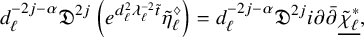 $$ \begin{align} d_{\ell}^{-2j-\alpha}\mathfrak{D}^{2j}\left(e^{d_{\ell}^2\lambda_{\ell}^{-2}\tilde{t}}\tilde{\eta}^\diamondsuit_{\ell}\right)=d_{\ell}^{-2j-\alpha}\mathfrak{D}^{2j}{i\partial\bar\partial}\underline{\tilde{\chi}^{*}_{\ell}}, \end{align} $$
on the same cylinder, which kills one contribution of
 $\underline{\tilde {\chi }^{*}_{\ell }}$
to (4.132).
$\underline{\tilde {\chi }^{*}_{\ell }}$
to (4.132).
Next, using (4.295) and the bounds (4.307) for
 $\tilde {\omega }^\sharp _{\ell }$
, we see that for any
$\tilde {\omega }^\sharp _{\ell }$
, we see that for any
 $a\geqslant 0$
, there is
$a\geqslant 0$
, there is
 $C>0$
such that
$C>0$
such that
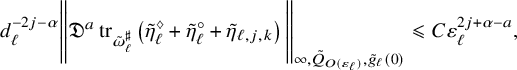 $$ \begin{align} d_{\ell}^{-2j-{\alpha}}\Bigg\| \mathfrak{D}^{a}\operatorname{tr}_{\tilde \omega_{\ell}^\sharp}\left(\tilde{\eta}_{\ell}^\diamondsuit+ \tilde{\eta}_{\ell}^\circ+\tilde{\eta}_{\ell,j,k}\right)\Bigg\|_{\infty,\tilde Q_{O(\varepsilon_{\ell})},\tilde g_{\ell}(0)}\leqslant C\varepsilon_{\ell}^{2j+{\alpha}-a}, \end{align} $$
 $$ \begin{align} d_{\ell}^{-2j-{\alpha}}\Bigg[ \mathfrak{D}^{a}\operatorname{tr}_{\tilde \omega_{\ell}^\sharp}\left(\tilde{\eta}_{\ell}^\diamondsuit+ \tilde{\eta}_{\ell}^\circ+\tilde{\eta}_{\ell,j,k}\right)\Bigg]_{{\beta},{\beta}/2,\tilde Q_{O(\varepsilon_{\ell})},\tilde g_{\ell}(0)}\leqslant C\varepsilon_{\ell}^{2j+{\alpha}-a-{\beta}}, \end{align} $$
while from (4.301), (4.322), (4.323) and (4.293), we have
 $$ \begin{align} d_{\ell}^{-2j-{\alpha}}\left\| \mathfrak{D}^{a}(\mathcal{E}_1+\mathcal{E}_2+\mathcal{E}_3)\right\|_{\infty,\tilde Q_{O(\varepsilon_{\ell})},\tilde g_{\ell}(0)}\leqslant C\varepsilon_{\ell}^{2j+{\alpha}-a}, \end{align} $$
 $$ \begin{align} d_{\ell}^{-2j-{\alpha}}\left[ \mathfrak{D}^{a}(\mathcal{E}_1+\mathcal{E}_2+\mathcal{E}_3)\right]_{{\beta},{\beta}/2,\tilde Q_{O(\varepsilon_{\ell})},\tilde g_{\ell}(0)}\leqslant C\varepsilon_{\ell}^{2j+{\alpha}-a-{\beta}}, \end{align} $$
and so using these in the PDE (4.216), we get
 $$ \begin{align} d_{\ell}^{-2j-{\alpha}}\left\| \mathfrak{D}^{a}(\partial_{\tilde t} \tilde{\rho}_{\ell}+d_{\ell}^2\lambda_{\ell}^{-2}\tilde{\rho}_{\ell})\right\|_{\infty,\tilde Q_{O(\varepsilon_{\ell})},\tilde g_{\ell}(0)}\leqslant C\varepsilon_{\ell}^{2j+{\alpha}-a}, \end{align} $$
 $$ \begin{align} d_{\ell}^{-2j-{\alpha}}\left[ \mathfrak{D}^{a}(\partial_{\tilde t} \tilde{\rho}_{\ell}+d_{\ell}^2\lambda_{\ell}^{-2}\tilde{\rho}_{\ell})\right]_{{\beta},{\beta}/2,\tilde Q_{O(\varepsilon_{\ell})},\tilde g_{\ell}(0)}\leqslant C\varepsilon_{\ell}^{2j+{\alpha}-a-{\beta}}. \end{align} $$
At this point, we want to deduce from this bounds for the fiber average of
 $\partial _{\tilde t} \tilde {\rho }_{\ell }+d_{\ell }^2\lambda _{\ell }^{-2}\tilde {\rho }_{\ell }$
, and this can be done using the following ‘non-cancellation’ estimate, stated in the hat picture, for a smooth time-dependent function f on
$\partial _{\tilde t} \tilde {\rho }_{\ell }+d_{\ell }^2\lambda _{\ell }^{-2}\tilde {\rho }_{\ell }$
, and this can be done using the following ‘non-cancellation’ estimate, stated in the hat picture, for a smooth time-dependent function f on
 $\hat {Q}_R$
(where the fiber average is
$\hat {Q}_R$
(where the fiber average is
 $\underline{f}=(\mathrm {pr}_B)_*(f\Psi _{\ell }^{*}\omega _F^n)$
) which states
$\underline{f}=(\mathrm {pr}_B)_*(f\Psi _{\ell }^{*}\omega _F^n)$
) which states
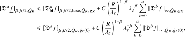 $$ \begin{align}\begin{aligned} [\mathfrak{D}^a\underline{f}] [\mathfrak{D}^a\underline{f}]_{{\beta},{\beta}/2,\hat{Q}_R}&\leqslant [\mathfrak{D}^a_{\mathbf{bt}}f]_{{\beta},{\beta}/2,\textrm{base},\hat{Q}_R, g_X} +C\left(\frac{R}{\lambda_{\ell}}\right)^{1-\beta}\lambda_{\ell}^{-\beta}\sum_{b=0}^a\|\mathfrak{D}^b f\|_{\infty,\hat{Q}_R,g_X}\\ &\leqslant [\mathfrak{D}^a f]_{{\beta},{\beta}/2,\hat{Q}_R, \hat{g}_{\ell}(0)} +C\left(\frac{R}{\lambda_{\ell}}\right)^{1-\beta}\lambda_{\ell}^{-\beta}\sum_{b=0}^a\|\mathfrak{D}^b f\|_{\infty,\hat{Q}_R,\hat{g}_{\ell}(0)}, \end{aligned} \end{align} $$
and which is proved exactly as [Reference Hein and Tosatti21, (4.199)], using Claims 2 and 3 there. We apply this in the tilde picture with
 $a=2j$
to the function
$a=2j$
to the function
 $\partial _{\tilde t} \tilde {\rho }_{\ell }+d_{\ell }^2\lambda _{\ell }^{-2}\tilde {\rho }_{\ell }$
, whose fiber average is by definition
$\partial _{\tilde t} \tilde {\rho }_{\ell }+d_{\ell }^2\lambda _{\ell }^{-2}\tilde {\rho }_{\ell }$
, whose fiber average is by definition
 $e^{-d_{\ell }^2\lambda _{\ell }^{-2}\tilde {t}}\partial _{\tilde {t}}\underline{\tilde {\chi }^{*}_{\ell }}$
, and we get
$e^{-d_{\ell }^2\lambda _{\ell }^{-2}\tilde {t}}\partial _{\tilde {t}}\underline{\tilde {\chi }^{*}_{\ell }}$
, and we get
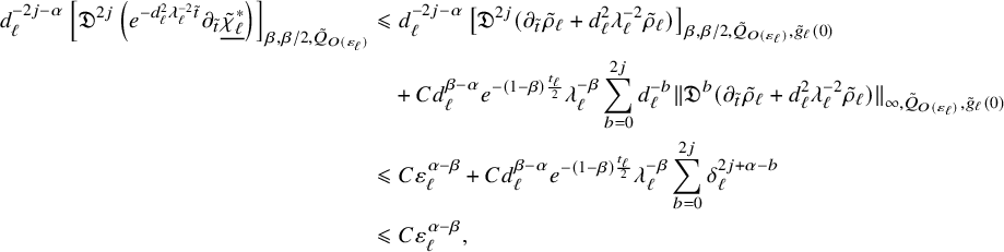 $$ \begin{align} \begin{aligned} d_{\ell}^{-2j-{\alpha}}\left[\mathfrak{D}^{2j}\left(e^{-d_{\ell}^2\lambda_{\ell}^{-2}\tilde{t}}\partial_{\tilde{t}}\underline{\tilde{\chi}^{*}_{\ell}}\right)\right]_{{\beta},{\beta}/2,\tilde Q_{O(\varepsilon_{\ell})}} &\leqslant d_{\ell}^{-2j-{\alpha}}\left[ \mathfrak{D}^{2j}(\partial_{\tilde t} \tilde{\rho}_{\ell}+d_{\ell}^2\lambda_{\ell}^{-2}\tilde{\rho}_{\ell})\right]_{{\beta},{\beta}/2,\tilde Q_{O(\varepsilon_{\ell})},\tilde{g}_{\ell}(0)}\\&\quad+Cd_{\ell}^{{\beta}-{\alpha}}e^{-(1-\beta)\frac{t_{\ell}}{2}}\lambda_{\ell}^{-\beta}\sum_{b=0}^{2j} d_{\ell}^{-b}\|\mathfrak{D}^b(\partial_{\tilde t} \tilde{\rho}_{\ell}+d_{\ell}^2\lambda_{\ell}^{-2}\tilde{\rho}_{\ell})\|_{\infty,\tilde{Q}_{O(\varepsilon_{\ell})},\tilde{g}_{\ell}(0)}\\&\leqslant C\varepsilon_{\ell}^{{\alpha}-{\beta}}+Cd_{\ell}^{{\beta}-{\alpha}}e^{-(1-\beta)\frac{t_{\ell}}{2}}\lambda_{\ell}^{-\beta}\sum_{b=0}^{2j}\delta_{\ell}^{2j+\alpha-b}\\&\leqslant C\varepsilon_{\ell}^{{\alpha}-{\beta}}, \end{aligned} \end{align} $$
using (4.331) and (4.332). Thus, if we take
 ${\beta }>{\alpha }$
, then the LHS of (4.334) is
${\beta }>{\alpha }$
, then the LHS of (4.334) is
 $o(1)$
, and so we get an
$o(1)$
, and so we get an
 $o(1)$
bound for the same
$o(1)$
bound for the same
 $C^{\beta ,\beta /2}$
seminorm on
$C^{\beta ,\beta /2}$
seminorm on
 $\tilde {Q}_R$
(
$\tilde {Q}_R$
(
 $R>1$
fixed), and hence,
$R>1$
fixed), and hence,
 $$ \begin{align} d_{\ell}^{-2j-{\alpha}}\left[ \mathfrak{D}^{2j}\left(e^{-d_{\ell}^2\lambda_{\ell}^{-2}\tilde{t}}\partial_{\tilde{t}}\underline{\tilde{\chi}^{*}_{\ell}}\right)\right]_{{\alpha},{\alpha}/2,\tilde Q_R,\tilde g_{\ell}(0)}=o(1), \end{align} $$
which thanks to the bounds in (4.153) implies that
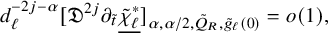 $$ \begin{align} d_{\ell}^{-2j-{\alpha}}[ \mathfrak{D}^{2j}\partial_{\tilde{t}}\underline{\tilde{\chi}^{*}_{\ell}}]_{{\alpha},{\alpha}/2,\tilde Q_R,\tilde g_{\ell}(0)}=o(1), \end{align} $$
which kills the other contribution of
 $\underline{\tilde {\chi }^{*}_{\ell }}$
to (4.132).
$\underline{\tilde {\chi }^{*}_{\ell }}$
to (4.132).
4.12.5 Killing the contribution of
$\tilde \psi _{\ell ,j,k}$

It remains to kill the contribution from
 $\tilde {\psi }_{\ell ,j,k}$
to (4.132). In contrast with [Reference Hein and Tosatti21, §4.10.7] where they had to kill the contribution from
$\tilde {\psi }_{\ell ,j,k}$
to (4.132). In contrast with [Reference Hein and Tosatti21, §4.10.7] where they had to kill the contribution from
 $d_{\ell }^{-2j-\alpha }\mathfrak {D}^{2j}{i\partial \bar \partial }\tilde {\psi }_{\ell ,j,k}$
, here we need to kill
$d_{\ell }^{-2j-\alpha }\mathfrak {D}^{2j}{i\partial \bar \partial }\tilde {\psi }_{\ell ,j,k}$
, here we need to kill
 $d_{\ell }^{-2j-\alpha }\mathfrak {D}^{2j+2}\tilde {\psi }_{\ell ,j,k}$
.
$d_{\ell }^{-2j-\alpha }\mathfrak {D}^{2j+2}\tilde {\psi }_{\ell ,j,k}$
.
From the definition of
 $\tilde {\rho }_{\ell }$
in (4.214), we have
$\tilde {\rho }_{\ell }$
in (4.214), we have
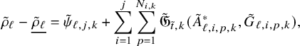 $$ \begin{align} \tilde{\rho}_{\ell}-\underline{\tilde{\rho}_{\ell}}=\tilde{\psi}_{\ell,j,k}+\sum_{i=1}^j\sum_{p=1}^{N_{i,k}}\tilde{\mathfrak{G}}_{\tilde{t},k}( \tilde A_{\ell,i,p,k}^{*},\tilde G_{\ell,i,p,k} ), \end{align} $$
and so using (4.332) and (4.334), together with the triangle inequality and the boundedness of
 $\mathbb {P}$
-parallel transport, gives
$\mathbb {P}$
-parallel transport, gives
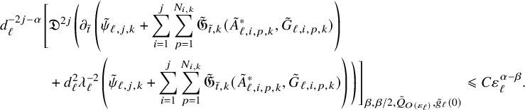 $$ \begin{align} \begin{aligned} d_{\ell}^{-2j-{\alpha}}\Bigg[&\mathfrak{D}^{2j}\Bigg(\partial_{\tilde{t}}\left(\tilde{\psi}_{\ell,j,k}+\sum_{i=1}^j\sum_{p=1}^{N_{i,k}}\tilde{\mathfrak{G}}_{\tilde{t},k}( \tilde A_{\ell,i,p,k}^{*},\tilde G_{\ell,i,p,k} )\right)\\ &+d_{\ell}^2\lambda_{\ell}^{-2}\left(\tilde{\psi}_{\ell,j,k}+\sum_{i=1}^j\sum_{p=1}^{N_{i,k}}\tilde{\mathfrak{G}}_{\tilde{t},k}( \tilde A_{\ell,i,p,k}^{*},\tilde G_{\ell,i,p,k} )\right)\Bigg)\Bigg]_{\beta,\beta/2,\tilde{Q}_{O(\varepsilon_{\ell})},\tilde{g}_{\ell}(0)}\leqslant C\varepsilon_{\ell}^{{\alpha}-{\beta}}. \end{aligned} \end{align} $$
Now thanks to (4.145) and (4.181), we can bound
 $$ \begin{align} d_{\ell}^2\lambda_{\ell}^{-2}d_{\ell}^{-2j-{\alpha}}\left[\mathfrak{D}^{2j}\left(\tilde{\psi}_{\ell,j,k}+\sum_{i=1}^j\sum_{p=1}^{N_{i,k}}\tilde{\mathfrak{G}}_{\tilde{t},k}( \tilde A_{\ell,i,p,k}^{*},\tilde G_{\ell,i,p,k} )\right) \right]_{\beta,\beta/2,\tilde{Q}_{O(\varepsilon_{\ell})},\tilde{g}_{\ell}(0)}\leqslant Cd_{\ell}^2\lambda_{\ell}^{-2}\varepsilon_{\ell}^{2+\alpha-\beta}=o(\varepsilon_{\ell}^{{\alpha}-{\beta}}), \end{align} $$
and so (4.338) implies
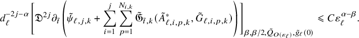 $$ \begin{align} \begin{aligned} d_{\ell}^{-2j-{\alpha}}\Bigg[&\mathfrak{D}^{2j}\partial_{\tilde{t}}\left(\tilde{\psi}_{\ell,j,k}+\sum_{i=1}^j\sum_{p=1}^{N_{i,k}}\tilde{\mathfrak{G}}_{\tilde{t},k}( \tilde A_{\ell,i,p,k}^{*},\tilde G_{\ell,i,p,k} )\right)\Bigg]_{\beta,\beta/2,\tilde{Q}_{O(\varepsilon_{\ell})},\tilde{g}_{\ell}(0)}\leqslant C\varepsilon_{\ell}^{{\alpha}-{\beta}}. \end{aligned} \end{align} $$
Next, from the bound (4.325), as well as the analogous bounds for lower derivatives of
 $\tilde {\eta }^\diamondsuit _{\ell }$
which come from (4.159), and the bounds (4.307) for
$\tilde {\eta }^\diamondsuit _{\ell }$
which come from (4.159), and the bounds (4.307) for
 $\tilde {\omega }^\sharp _{\ell }$
, we see that
$\tilde {\omega }^\sharp _{\ell }$
, we see that
 $$ \begin{align} d_{\ell}^{-2j-{\alpha}}[ \mathfrak{D}^{2j}\operatorname{tr}_{\tilde \omega_{\ell}^\sharp}\tilde{\eta}_{\ell}^\diamondsuit]_{{\beta},{\beta}/2,\tilde Q_{O(\varepsilon_{\ell})},\tilde g_{\ell}(0)}\leqslant C\varepsilon_{\ell}^{{\alpha}-{\beta}}, \end{align} $$
and this together with (4.328) gives
 $$ \begin{align} d_{\ell}^{-2j-{\alpha}}[ \mathfrak{D}^{2j}\operatorname{tr}_{\tilde \omega_{\ell}^\sharp}\left(\tilde{\eta}_{\ell}^\circ+\tilde{\eta}_{\ell,j,k}\right)]_{{\beta},{\beta}/2,\tilde Q_{O(\varepsilon_{\ell})},\tilde g_{\ell}(0)}\leqslant C\varepsilon_{\ell}^{{\alpha}-{\beta}}, \end{align} $$
which together with (4.340) gives
 $$ \begin{align} \begin{aligned} d_{\ell}^{-2j-{\alpha}}\Bigg[&\mathfrak{D}^{2j}\left(\partial_{\tilde{t}}-\Delta_{\tilde{\omega}^\sharp_{\ell}}\right)\left(\tilde{\psi}_{\ell,j,k}+\sum_{i=1}^j\sum_{p=1}^{N_{i,k}}\tilde{\mathfrak{G}}_{\tilde{t},k}( \tilde A_{\ell,i,p,k}^{*},\tilde G_{\ell,i,p,k} )\right)\Bigg]_{\beta,\beta/2,\tilde{Q}_{O(\varepsilon_{\ell})},\tilde{g}_{\ell}(0)}\leqslant C\varepsilon_{\ell}^{{\alpha}-{\beta}}. \end{aligned} \end{align} $$
This estimate can be inserted in the Schauder estimates in Proposition 2.8 (as usual by first going to the check picture, and then changing the result back to the tilde picture), with radii both
 $O(\varepsilon _{\ell })$
,
$O(\varepsilon _{\ell })$
,
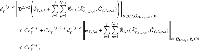 $$ \begin{align} \begin{aligned} d_{\ell}^{-2j-{\alpha}}\Bigg[&\mathfrak{D}^{2j+2}\left(\tilde{\psi}_{\ell,j,k}+\sum_{i=1}^j\sum_{p=1}^{N_{i,k}}\tilde{\mathfrak{G}}_{\tilde{t},k}( \tilde A_{\ell,i,p,k}^{*},\tilde G_{\ell,i,p,k} )\right)\Bigg]_{\beta,\beta/2,\tilde{Q}_{O(\varepsilon_{\ell})},\tilde{g}_{\ell}(0)}\\ &\leqslant C\varepsilon_{\ell}^{{\alpha}-{\beta}}+C\varepsilon_{\ell}^{-2j-2-\beta}d_{\ell}^{-2j-{\alpha}}\left\|\tilde{\psi}_{\ell,j,k} +\sum_{i=1}^j\sum_{p=1}^{N_{i,k}}\tilde{\mathfrak{G}}_{\tilde{t},k}( \tilde A_{\ell,i,p,k}^{*},\tilde G_{\ell,i,p,k} )\right\|_{\infty,\tilde{Q}_{O(\varepsilon_{\ell})},\tilde{g}_{\ell}(0)}\\ &\leqslant C\varepsilon_{\ell}^{{\alpha}-{\beta}}, \end{aligned} \end{align} $$
where we used the bounds (4.145) and (4.181) for the
 $L^\infty $
norm. As usual, taking
$L^\infty $
norm. As usual, taking
 $\beta>\alpha $
, this implies an
$\beta>\alpha $
, this implies an
 $o(1)$
bound for the
$o(1)$
bound for the
 $C^{{\beta },{\beta }/2}$
seminorm on
$C^{{\beta },{\beta }/2}$
seminorm on
 $\tilde {Q}_{O(\varepsilon _{\ell })}$
, hence on
$\tilde {Q}_{O(\varepsilon _{\ell })}$
, hence on
 $\tilde {Q}_{2}$
, and hence also an
$\tilde {Q}_{2}$
, and hence also an
 $o(1)$
bound for the
$o(1)$
bound for the
 $C^{{\alpha },{\alpha }/2}$
seminorm on
$C^{{\alpha },{\alpha }/2}$
seminorm on
 $\tilde {Q}_{2}$
; that is,
$\tilde {Q}_{2}$
; that is,
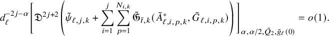 $$ \begin{align} d_{\ell}^{-2j-{\alpha}}\Bigg[\mathfrak{D}^{2j+2}\left(\tilde{\psi}_{\ell,j,k}+\sum_{i=1}^j\sum_{p=1}^{N_{i,k}}\tilde{\mathfrak{G}}_{\tilde{t},k}( \tilde A_{\ell,i,p,k}^{*},\tilde G_{\ell,i,p,k} )\right)\Bigg]_{{\alpha},{\alpha}/2,\tilde{Q}_{2},\tilde{g}_{\ell}(0)}=o(1). \end{align} $$
Next, we claim that
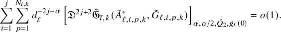 $$ \begin{align} \displaystyle \sum_{i=1}^j\sum_{p=1}^{N_{i,k}}d_{\ell}^{-2j-{\alpha}} \left[\mathfrak{D}^{2j+2} \tilde{\mathfrak{G}}_{\tilde{t},k}( \tilde A_{\ell,i,p,k}^{*},\tilde G_{\ell,i,p,k} )\right]_{{\alpha},{\alpha}/2,\tilde Q_2,\tilde g_{\ell}(0)}=o(1). \end{align} $$
The argument is identical to the deduction of (4.181) except we now use the improved parabolic Hölder seminorm from (4.281) instead of that from blowup argument. By applying (3.1), we have
 $$ \begin{align} \tilde{\mathfrak{G}}_{\tilde{t},k}( \tilde A_{\ell,i,p,k}^{*},\tilde G_{\ell,i,p,k} )=\sum_{\iota=0}^{2k}\sum_{q=\lceil\frac{\iota}{2}\rceil}^ke^{-qd_{\ell}^2\lambda_{\ell}^{-2}\tilde t-(q-\frac{\iota}{2})t_{\ell}} \varepsilon_{\ell}^{\iota} \cdot \tilde \Phi_{\iota,q}(\tilde G_{i,p,k})\circledast {\mathbb{D}}^\iota \tilde A_{\ell,i,p,k}^{*}. \end{align} $$
so that
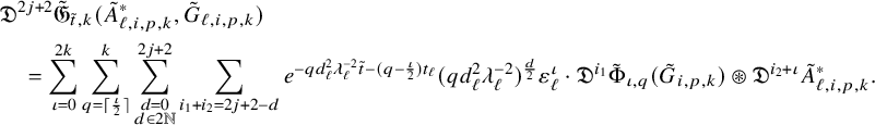 $$ \begin{align} \begin{aligned} &\mathfrak{D}^{2j+2}\tilde{\mathfrak{G}}_{\tilde{t},k}( \tilde A_{\ell,i,p,k}^{*},\tilde G_{\ell,i,p,k} )\\& \quad = \sum_{\iota=0}^{2k}\sum_{q=\lceil\frac{\iota}{2}\rceil}^{k} \sum_{\substack{d=0\\d\in 2\mathbb{N}}}^{2j+2} \sum_{i_1+i_2=2j+2-d} e^{-qd_{\ell}^2\lambda_{\ell}^{-2}\tilde t-(q-\frac{\iota}{2})t_{\ell}} (qd_{\ell}^2\lambda_{\ell}^{-2})^{\frac{d}{2}}\varepsilon_{\ell}^{\iota} \cdot \mathfrak{D}^{i_1}\tilde \Phi_{\iota,q}(\tilde G_{i,p,k})\circledast \mathfrak{D}^{i_2+\iota} \tilde A_{\ell,i,p,k}^{*}. \end{aligned} \end{align} $$
To estimate it, we need the following simple bounds from [Reference Hein and Tosatti21, (4.302)–(4.303)]
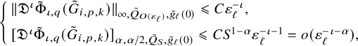 $$ \begin{align} \left\{ \begin{array}{ll} \|\mathfrak{D}^\iota \tilde \Phi_{\iota,q}(\tilde G_{i,p,k})\|_{\infty, \tilde Q_{O(\varepsilon_{\ell})},\tilde g_{\ell}(0)}\leqslant C\varepsilon_{\ell}^{-\iota},\\[2mm] [\mathfrak{D}^\iota \tilde \Phi_{\iota,q}(\tilde G_{i,p,k})]_{{\alpha},{\alpha}/2, \tilde Q_{S},\tilde g_{\ell}(0)}\leqslant CS^{1-{\alpha}}\varepsilon_{\ell}^{-\iota-1}=o (\varepsilon_{\ell}^{-\iota-{\alpha}}), \end{array} \right. \end{align} $$
for all
 $\iota \geqslant 0$
,
$\iota \geqslant 0$
,
 ${\alpha }\in (0,1)$
and fixed
${\alpha }\in (0,1)$
and fixed
 $S>1$
.
$S>1$
.
Transferring (4.178) to the tilde picture,
 $$ \begin{align} d_{\ell}^{-\iota+2}\| \mathfrak{D}^\iota \tilde A_{\ell,i,p,k}^{*}\|_{\infty,\tilde Q_{O(\varepsilon_{\ell})},\tilde g_{\ell}(0)}\leqslant C\delta_{\ell}^{2+2j-\iota+{\alpha}}=o(\delta_{\ell}^{2+2j-\iota}), \end{align} $$
for all
 $0\leqslant \iota \leqslant 2k+2+2j$
. Putting
$0\leqslant \iota \leqslant 2k+2+2j$
. Putting
 ${\beta }>{\alpha }$
in (4.281) yields
${\beta }>{\alpha }$
in (4.281) yields
 $$ \begin{align} d_{\ell}^{-\iota+2-{\alpha}}[\mathfrak{D}^\iota \tilde A_{\ell,i,p,k}^{*}]_{{\beta},{\beta}/2,\tilde Q_{O(\varepsilon_{\ell})},\tilde g_{\ell}(0)}\leqslant C \varepsilon_{\ell}^{{\alpha}-{\beta}} \delta_{\ell}^{2j-\iota+2}=o(\delta_{\ell}^{2+2j-\iota}), \end{align} $$
for all
 $\iota \geqslant 2j$
and thus implies
$\iota \geqslant 2j$
and thus implies
 $$ \begin{align} d_{\ell}^{-\iota+2-{\alpha}}[\mathfrak{D}^\iota \tilde A_{\ell,i,p,k}^{*}]_{{\alpha},{\alpha}/2,\tilde Q_{2},\tilde g_{\ell}(0)}\leqslant C \varepsilon_{\ell}^{{\alpha}-{\beta}} \delta^{2+2j-\iota}_{\ell} =o(\delta_{\ell}^{2+2j-\iota}), \end{align} $$
for all
 $2j\leqslant \iota \leqslant 2j+2+2k$
while for
$2j\leqslant \iota \leqslant 2j+2+2k$
while for
 $0\leqslant \iota \leqslant 2j$
, we have from (4.163) that
$0\leqslant \iota \leqslant 2j$
, we have from (4.163) that
 $$ \begin{align} d_{\ell}^{2-\iota-{\alpha}} [\mathfrak{D}^\iota \tilde A_{\ell,i,p,k}^{*}]_{{\alpha},{\alpha}/2,\tilde Q_2,\tilde g_{\ell}(0)}\leqslant C\delta_{\ell}^2 d_{\ell}^{2j-\iota}=o(\delta_{\ell}^{2+2j-\iota}), \end{align} $$
since
 $\varepsilon _{\ell }\to +\infty $
.
$\varepsilon _{\ell }\to +\infty $
.
We now estimate (4.348) using the above estimates of each terms:
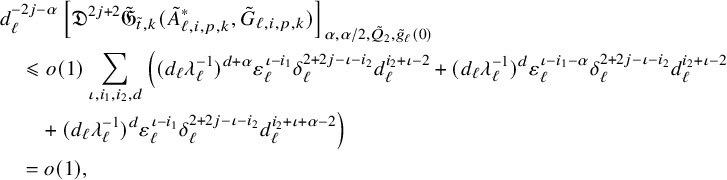 $$ \begin{align} \begin{aligned} &d_{\ell}^{-2j-{\alpha}}\left[\mathfrak{D}^{2j+2}\tilde{\mathfrak{G}}_{\tilde{t},k}( \tilde A_{\ell,i,p,k}^{*},\tilde G_{\ell,i,p,k})\right]_{{\alpha},{\alpha}/2,\tilde Q_2,\tilde g_{\ell}(0)}\\&\quad\leqslant o(1)\sum_{\iota,i_1,i_2,d} \Big( (d_{\ell}\lambda_{\ell}^{-1})^{d+{\alpha}}\varepsilon_{\ell}^{\iota-i_1} \delta_{\ell}^{2+2j-\iota-i_2} d_{\ell}^{i_2+\iota-2} +(d_{\ell}\lambda_{\ell}^{-1})^{d}\varepsilon_{\ell}^{\iota-i_1-{\alpha}} \delta_{\ell}^{2+2j-\iota-i_2}d_{\ell}^{i_2+\iota-2}\\&\quad\quad +(d_{\ell}\lambda_{\ell}^{-1})^{d}\varepsilon_{\ell}^{\iota-i_1} \delta_{\ell}^{2+2j-\iota-i_2} d_{\ell}^{i_2+\iota+{\alpha}-2} \Big)\\&\quad=o(1), \end{aligned} \end{align} $$
which proves (4.346). Combining it with (4.345), and using the triangle inequality gives
 $$ \begin{align} d_{\ell}^{-2j-\alpha}[\mathfrak{D}^{2j+2}\tilde{\psi}_{\ell,j,k}]_{{\alpha},{\alpha}/2,\tilde{Q}_{2},\tilde g_{\ell}(0)}=o(1), \end{align} $$
which kills the contribution of
 $\tilde {\psi }_{\ell ,j,k}$
in (4.132). In conclusion, all terms that appear on the right-hand side of (4.132) converge to zero, which gives a contradiction and finally concludes Subcase A.
$\tilde {\psi }_{\ell ,j,k}$
in (4.132). In conclusion, all terms that appear on the right-hand side of (4.132) converge to zero, which gives a contradiction and finally concludes Subcase A.
4.13 Subcase B:
$\varepsilon _{\ell }\to \varepsilon _\infty>0$

Without loss of generality, we will assume that
 $\varepsilon _\infty =1$
. By (4.144), (4.145) and [Reference Hein and Tosatti21, Lemma 2.6], we see that
$\varepsilon _\infty =1$
. By (4.144), (4.145) and [Reference Hein and Tosatti21, Lemma 2.6], we see that
 $d_{\ell }^{-2j-{\alpha }}\tilde {\psi }_{\ell ,j,k}$
converges in
$d_{\ell }^{-2j-{\alpha }}\tilde {\psi }_{\ell ,j,k}$
converges in
 $C^{2j+2+{\beta },j+1+{\beta }/2}_{\mathrm {loc}}$
to a function
$C^{2j+2+{\beta },j+1+{\beta }/2}_{\mathrm {loc}}$
to a function
 $\tilde {\psi }_{\infty ,j,k}\in C^{2j+2+{\alpha },j+1+{\alpha }/2}_{\mathrm {loc}}$
defined on
$\tilde {\psi }_{\infty ,j,k}\in C^{2j+2+{\alpha },j+1+{\alpha }/2}_{\mathrm {loc}}$
defined on
 $\mathbb {C}^m\times Y\times (-\infty ,0]$
, for all
$\mathbb {C}^m\times Y\times (-\infty ,0]$
, for all
 $0<{\beta }<{\alpha }$
, while (4.153) gives us that
$0<{\beta }<{\alpha }$
, while (4.153) gives us that
 $d_{\ell }^{-2j-{\alpha }}\partial _{\tilde t}\underline{\tilde {\chi }_{\ell }^{*}}$
and
$d_{\ell }^{-2j-{\alpha }}\partial _{\tilde t}\underline{\tilde {\chi }_{\ell }^{*}}$
and
 $d_{\ell }^{-2j-{\alpha }}{i\partial \bar \partial }\underline{\tilde {\chi }_{\ell }^{*}}$
converge in
$d_{\ell }^{-2j-{\alpha }}{i\partial \bar \partial }\underline{\tilde {\chi }_{\ell }^{*}}$
converge in
 $C_{\mathrm { loc}}^{2j+{\beta },j+{\beta }/2}$
for all
$C_{\mathrm { loc}}^{2j+{\beta },j+{\beta }/2}$
for all
 $0<{\beta }<{\alpha }$
to a function
$0<{\beta }<{\alpha }$
to a function
 $u_\infty \in C^{2j+{\alpha },j+{\alpha }/2}_{\mathrm {loc}}$
and to a
$u_\infty \in C^{2j+{\alpha },j+{\alpha }/2}_{\mathrm {loc}}$
and to a
 $(1,1)$
form
$(1,1)$
form
 $\eta _\infty \in C^{2j+{\alpha },j+{\alpha }/2}_{\mathrm {loc}}$
, respectively, on
$\eta _\infty \in C^{2j+{\alpha },j+{\alpha }/2}_{\mathrm {loc}}$
, respectively, on
 $\mathbb {C}^m\times (-\infty ,0]$
. Using again (4.153), we also have that
$\mathbb {C}^m\times (-\infty ,0]$
. Using again (4.153), we also have that
 $d_{\ell }^{-2j-{\alpha }}e^{-d_{\ell }^2\lambda _{\ell }^{-2}\tilde t}\partial _{\tilde t}\underline{\tilde \chi _{\ell }^{*} }\to u_\infty $
in
$d_{\ell }^{-2j-{\alpha }}e^{-d_{\ell }^2\lambda _{\ell }^{-2}\tilde t}\partial _{\tilde t}\underline{\tilde \chi _{\ell }^{*} }\to u_\infty $
in
 $C_{\mathrm {loc}}^{2j+{\beta },j+{\beta }/2}$
and
$C_{\mathrm {loc}}^{2j+{\beta },j+{\beta }/2}$
and
 $d_{\ell }^{-2j-{\alpha }}e^{-d_{\ell }^2\lambda _{\ell }^{-2}\tilde t}{i\partial \bar \partial }\underline{\tilde \chi _{\ell }^{*} }\to \eta _\infty $
in
$d_{\ell }^{-2j-{\alpha }}e^{-d_{\ell }^2\lambda _{\ell }^{-2}\tilde t}{i\partial \bar \partial }\underline{\tilde \chi _{\ell }^{*} }\to \eta _\infty $
in
 $C_{\mathrm {loc}}^{2j+{\beta },j+{\beta }/2}$
. Moreover, when
$C_{\mathrm {loc}}^{2j+{\beta },j+{\beta }/2}$
. Moreover, when
 $j\geqslant 1$
, we have
$j\geqslant 1$
, we have
 $$ \begin{align} {i\partial\bar\partial} u_\infty=\partial_{\tilde t}\eta_\infty. \end{align} $$
From (4.144), (4.145), (4.153), (4.191), we see that
 $\tilde {\psi }_{\infty ,j,k}=O(r^{2j+2+{\alpha }})$
,
$\tilde {\psi }_{\infty ,j,k}=O(r^{2j+2+{\alpha }})$
,
 $u_\infty =O(r^{2j+{\alpha }})$
,
$u_\infty =O(r^{2j+{\alpha }})$
,
 $\eta _\infty =O(r^{2j+{\alpha }}),$
and
$\eta _\infty =O(r^{2j+{\alpha }}),$
and
 $\tilde {\eta }_\infty ^\circ =O(r^{2j+{\alpha }})$
where
$\tilde {\eta }_\infty ^\circ =O(r^{2j+{\alpha }})$
where
 $r=|z|+\sqrt {|t|}$
.
$r=|z|+\sqrt {|t|}$
.
By (4.164), (4.163) and (4.168), the functions
 $d_{\ell }^{-2j-{\alpha }}\tilde A_{\ell ,i,p,k}^{*}$
converge to limiting functions
$d_{\ell }^{-2j-{\alpha }}\tilde A_{\ell ,i,p,k}^{*}$
converge to limiting functions
 $\tilde A_{\infty ,i,p,k}^{*}$
from the base
$\tilde A_{\infty ,i,p,k}^{*}$
from the base
 $\mathbb {C}^m$
in
$\mathbb {C}^m$
in
 $C_{\mathrm {loc}}^{2j+2+2k+{\beta },j+1+2k+{\beta }/2}$
for any
$C_{\mathrm {loc}}^{2j+2+2k+{\beta },j+1+2k+{\beta }/2}$
for any
 $0<{\beta }<{\alpha }$
while
$0<{\beta }<{\alpha }$
while
 $\tilde G_{i,p,k}$
converge locally uniformly smoothly to functions
$\tilde G_{i,p,k}$
converge locally uniformly smoothly to functions
 $\tilde G_{\infty ,i,p,k}$
pulled back from Y. Using (4.181), we see that the functions
$\tilde G_{\infty ,i,p,k}$
pulled back from Y. Using (4.181), we see that the functions
 $d_{\ell }^{-2j-{\alpha }}\tilde {\mathfrak {G}}_{\tilde {t},k}(\tilde {A}_{\ell ,i,p,k}^{*},\tilde {G}_{\ell ,i,p,k})$
converge in
$d_{\ell }^{-2j-{\alpha }}\tilde {\mathfrak {G}}_{\tilde {t},k}(\tilde {A}_{\ell ,i,p,k}^{*},\tilde {G}_{\ell ,i,p,k})$
converge in
 $C^{2j+2+{\beta },j+1+{\beta }/2}_{\mathrm {loc}}$
to a function which, thanks to [Reference Hein and Tosatti21, (4.310)], is given by
$C^{2j+2+{\beta },j+1+{\beta }/2}_{\mathrm {loc}}$
to a function which, thanks to [Reference Hein and Tosatti21, (4.310)], is given by
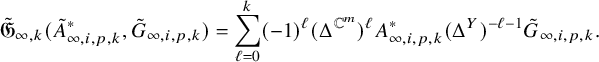 $$ \begin{align} \tilde{\mathfrak{G}}_{\infty,k}(\tilde A_{\infty,i,p,k}^{*},\tilde G_{\infty,i,p,k})=\sum_{\ell=0}^{k}(-1)^\ell (\Delta^{\mathbb{C}^m})^\ell A_{\infty,i,p,k}^{*} (\Delta^Y)^{-\ell-1}\tilde G_{\infty,i,p,k}. \end{align} $$
By (4.158) and (4.200), the metrics
 $\tilde g^\sharp _{\ell }(t)\to g_P=g_{\mathbb {C}^m}+g_{Y,z_\infty =0}$
locally smoothly where
$\tilde g^\sharp _{\ell }(t)\to g_P=g_{\mathbb {C}^m}+g_{Y,z_\infty =0}$
locally smoothly where
 $g_{\mathbb {C}^m}$
equals
$g_{\mathbb {C}^m}$
equals
 $g_{\mathrm {can}}|_{z=z_\infty =0}$
.
$g_{\mathrm {can}}|_{z=z_\infty =0}$
.
Recall from (4.216) that
 $$ \begin{align} d_{\ell}^{-2j-{\alpha}}\left(\left(\partial_{\tilde t}- \Delta_{\tilde{\omega}^\sharp_{\ell}}\right)\tilde{\rho}_{\ell}+d_{\ell}^2\lambda_{\ell}^{-2}\tilde{\rho}_{\ell}\right)=d_{\ell}^{-2j-{\alpha}}(\mathcal{E}_1+\mathcal{E}_2+\mathcal{E}_3), \end{align} $$
where
 $\tilde {\rho }_{\ell }$
is given by (4.214). From (4.144), (4.145), (4.157) and (4.179), it follows that
$\tilde {\rho }_{\ell }$
is given by (4.214). From (4.144), (4.145), (4.157) and (4.179), it follows that
 $$ \begin{align} d_{\ell}^{-2j-{\alpha}}d_{\ell}^2\lambda_{\ell}^{-2}\tilde{\rho}_{\ell}\to 0, \end{align} $$
in
 $C^0_{\mathrm {loc}}$
, so as
$C^0_{\mathrm {loc}}$
, so as
 $\ell \to +\infty $
the LHS of (4.358) converges to
$\ell \to +\infty $
the LHS of (4.358) converges to
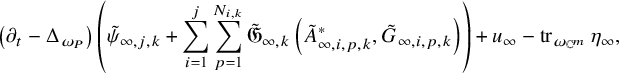 $$ \begin{align} \left(\partial_{t}- \Delta_{\omega_P}\right)\left(\tilde{\psi}_{\infty,j,k}+\sum_{i=1}^j\sum_{p=1}^{N_{i,k}} \tilde{\mathfrak{G}}_{\infty,k}\left( \tilde A_{\infty,i,p,k}^{*},\tilde G_{\infty,i,p,k} \right) \right)+u_\infty-\operatorname{tr}_{\omega_{\mathbb{C}^m}}\eta_\infty, \end{align} $$
while at the same time, thanks to (4.219), the LHS of (4.358) is forced to be a polynomial
 $\mathcal {F}$
in the
$\mathcal {F}$
in the
 $(z,t)$
variables, of (spacetime) degree at most
$(z,t)$
variables, of (spacetime) degree at most
 $2j$
, with coefficients that are functions on Y, namely
$2j$
, with coefficients that are functions on Y, namely
 $$ \begin{align} \mathcal{F}(z,y,t)=\sum_{|p|+2q\leqslant 2j} H_{p,q}(y) z^p t^q, \end{align} $$
for some smooth functions
 $H_{p,q}$
pullback from the fiber Y, where here again we treat z as real variables. Plugging (4.361) into (4.360), and taking the fiberwise average, gives
$H_{p,q}$
pullback from the fiber Y, where here again we treat z as real variables. Plugging (4.361) into (4.360), and taking the fiberwise average, gives
 $$ \begin{align} u_\infty-\operatorname{tr}_{\omega_{\mathbb{C}^m}}\eta_\infty=Q, \end{align} $$
where Q is a polynomial in the
 $(z,t)$
variables of degree at most
$(z,t)$
variables of degree at most
 $2j$
. But thanks to the jet subtractions,
$2j$
. But thanks to the jet subtractions,
 $u_\infty $
and
$u_\infty $
and
 $\eta _\infty $
have vanishing
$\eta _\infty $
have vanishing
 $2j$
parabolic jet at
$2j$
parabolic jet at
 $(z,t)=(0,0)$
, so
$(z,t)=(0,0)$
, so
 $$ \begin{align} u_\infty-\operatorname{tr}_{\omega_{\mathbb{C}^m}}\eta_\infty=0, \end{align} $$
on
 $\mathbb {C}^m\times (-\infty ,0]$
.
$\mathbb {C}^m\times (-\infty ,0]$
.
We now claim that
 $u_\infty $
and
$u_\infty $
and
 $\eta _\infty $
are both identically zero. First, we assume that
$\eta _\infty $
are both identically zero. First, we assume that
 $j=0$
. In this case, we can use (4.268) and see that
$j=0$
. In this case, we can use (4.268) and see that
 $u_\infty $
is a constant in space-time, and hence identically zero. At this point, we can argue similarly as in subcase A to show that
$u_\infty $
is a constant in space-time, and hence identically zero. At this point, we can argue similarly as in subcase A to show that
 $\eta _\infty $
also vanishes identically: first, we show that
$\eta _\infty $
also vanishes identically: first, we show that
 $\eta _\infty $
is time-independent, by arguing similarly to (4.270), noting that for any
$\eta _\infty $
is time-independent, by arguing similarly to (4.270), noting that for any
 $\tilde {z}\in \mathbb {C}^m$
and
$\tilde {z}\in \mathbb {C}^m$
and
 $\tilde {t},\tilde {t}'\leqslant 0$
,
$\tilde {t},\tilde {t}'\leqslant 0$
,
 $$ \begin{align} d_{\ell}^{-{\alpha}}{i\partial\bar\partial}\underline{\tilde{\chi}^{*}_{\ell}}(\tilde{z},\tilde{t})-d_{\ell}^{-{\alpha}}{i\partial\bar\partial}\underline{\tilde{\chi}^{*}_{\ell}}(\tilde{z},\tilde{t}')={i\partial\bar\partial} \int_{\tilde{t}'}^{\tilde{t}}\left(d_{\ell}^{-{\alpha}}\partial_{\tilde{t}}\underline{\tilde{\chi}^{*}_{\ell}}\right)(\tilde{z},\tilde{s})d\tilde{s}, \end{align} $$
and since
 $\int _{\tilde {t}'}^{\tilde {t}}\left(d_{\ell }^{-{\alpha }}\partial _{\tilde {t}}\underline{\tilde {\chi }^{*}_{\ell }}\right)(\tilde {z},\tilde {s})d\tilde {s}\to 0$
locally uniformly (from
$\int _{\tilde {t}'}^{\tilde {t}}\left(d_{\ell }^{-{\alpha }}\partial _{\tilde {t}}\underline{\tilde {\chi }^{*}_{\ell }}\right)(\tilde {z},\tilde {s})d\tilde {s}\to 0$
locally uniformly (from
 $u_\infty \equiv 0$
), it follows that the RHS of (4.364) goes to
$u_\infty \equiv 0$
), it follows that the RHS of (4.364) goes to
 $0$
weakly, and since the LHS converges in
$0$
weakly, and since the LHS converges in
 $C^\beta _{\mathrm {loc}}$
to
$C^\beta _{\mathrm {loc}}$
to
 $\eta _\infty (\tilde {z},\tilde {t})-\eta _\infty (\tilde {z},\tilde {t}')$
, this must be identically zero as claimed.
$\eta _\infty (\tilde {z},\tilde {t})-\eta _\infty (\tilde {z},\tilde {t}')$
, this must be identically zero as claimed.
We can then write
 $\eta _\infty ={i\partial \bar \partial } v_\infty $
, where
$\eta _\infty ={i\partial \bar \partial } v_\infty $
, where
 $v_\infty \in C^{2+{\alpha }}_{\mathrm {loc}}(\mathbb {C}^m)$
is time-independent and
$v_\infty \in C^{2+{\alpha }}_{\mathrm {loc}}(\mathbb {C}^m)$
is time-independent and
 $\Delta _{g_{\mathbb {C}^m}}v_\infty =0$
, so
$\Delta _{g_{\mathbb {C}^m}}v_\infty =0$
, so
 $v_\infty $
is smooth and
$v_\infty $
is smooth and
 $|{i\partial \bar \partial } v_\infty |=O(|z|^{\alpha })$
. The Liouville Theorem applied to each component of
$|{i\partial \bar \partial } v_\infty |=O(|z|^{\alpha })$
. The Liouville Theorem applied to each component of
 ${i\partial \bar \partial } v_\infty $
then implies that
${i\partial \bar \partial } v_\infty $
then implies that
 $\eta _\infty $
has constant coefficients; hence, it vanishes identically since its value at
$\eta _\infty $
has constant coefficients; hence, it vanishes identically since its value at
 $(0,0)$
vanishes.
$(0,0)$
vanishes.
Next, we assume
 $j\geqslant 1$
. We can then differentiate (4.363) and use (4.356) to see that
$j\geqslant 1$
. We can then differentiate (4.363) and use (4.356) to see that
 $$ \begin{align} \begin{aligned} \partial_{t}u_\infty &=\operatorname{tr}_{\mathbb{C}^m}\partial_{t} \eta_\infty=\operatorname{tr}_{\mathbb{C}^m}{i\partial\bar\partial} u_\infty=\Delta_{\mathbb{C}^m}u_\infty, \end{aligned} \end{align} $$
so
 $u_\infty $
solves the heat equation on
$u_\infty $
solves the heat equation on
 $(-\infty ,0]\times \mathbb {C}^m$
, and
$(-\infty ,0]\times \mathbb {C}^m$
, and
 $|\mathfrak {D}^{\iota }u_\infty |=O(r^{2j+{\alpha }-\iota })$
where
$|\mathfrak {D}^{\iota }u_\infty |=O(r^{2j+{\alpha }-\iota })$
where
 $r=|x|+\sqrt {t}$
for
$r=|x|+\sqrt {t}$
for
 $0\leqslant \iota \leqslant 2j$
by (4.153). By applying Liouville Theorem for ancient heat equation to
$0\leqslant \iota \leqslant 2j$
by (4.153). By applying Liouville Theorem for ancient heat equation to
 $\mathfrak {D}^{2j}u_\infty $
, we see that
$\mathfrak {D}^{2j}u_\infty $
, we see that
 $u_\infty $
must be a space-time polynomial of degree at most
$u_\infty $
must be a space-time polynomial of degree at most
 $2j$
, and hence,
$2j$
, and hence,
 $u_\infty \equiv 0$
since its parabolic
$u_\infty \equiv 0$
since its parabolic
 $2j$
-jet at
$2j$
-jet at
 $(0,0)$
vanishes. Going back to (4.356), it then follows that
$(0,0)$
vanishes. Going back to (4.356), it then follows that
 $\eta _\infty $
is time-independent, and it is clearly of the form
$\eta _\infty $
is time-independent, and it is clearly of the form
 $\eta _\infty ={i\partial \bar \partial } v_\infty $
for some time-independent function
$\eta _\infty ={i\partial \bar \partial } v_\infty $
for some time-independent function
 $v_\infty \in C^{2j+2+{\alpha }}_{\mathrm {loc}}(\mathbb {C}^m)$
. From (4.363), we see that
$v_\infty \in C^{2j+2+{\alpha }}_{\mathrm {loc}}(\mathbb {C}^m)$
. From (4.363), we see that
 $v_\infty $
is harmonic. Since
$v_\infty $
is harmonic. Since
 $|{\mathbb {D}}^{2j}\eta _\infty |=O(|z|^{\alpha })$
, the Liouville Theorem in [Reference Hein and Tosatti20, Proposition 3.12] then shows that the coefficients of
$|{\mathbb {D}}^{2j}\eta _\infty |=O(|z|^{\alpha })$
, the Liouville Theorem in [Reference Hein and Tosatti20, Proposition 3.12] then shows that the coefficients of
 $\eta _\infty $
are polynomials of degree at most
$\eta _\infty $
are polynomials of degree at most
 $2j$
, and since these coefficients have vanishing
$2j$
, and since these coefficients have vanishing
 $2j$
-jet at the origin, this implies that
$2j$
-jet at the origin, this implies that
 $\eta _\infty $
vanishes identically.
$\eta _\infty $
vanishes identically.
Now that we know that
 $u_\infty \equiv 0, \eta _\infty \equiv 0$
, we can return to (4.360), (4.361) and get
$u_\infty \equiv 0, \eta _\infty \equiv 0$
, we can return to (4.360), (4.361) and get
 $$ \begin{align} \begin{aligned} &\quad \left(\partial_{t}-\Delta_{\omega_P}\right)\left(\tilde{\psi}_{\infty,j,k}+\sum_{i=1}^j\sum_{p=1}^{N_{i,k}} \tilde{\mathfrak{G}}_{\infty,k}\left( \tilde A_{\infty,i,p,k}^{*},\tilde G_{\infty,i,p,k} \right) \right)=\mathcal{F}. \end{aligned} \end{align} $$
Recall from (4.358) and the discussion after it that
 $d_{\ell }^{-2j-{\alpha }}(\mathcal {E}_1+\mathcal {E}_2+\mathcal {E}_3)\to \mathcal {F}$
locally uniformly. From (4.220), we see that
$d_{\ell }^{-2j-{\alpha }}(\mathcal {E}_1+\mathcal {E}_2+\mathcal {E}_3)\to \mathcal {F}$
locally uniformly. From (4.220), we see that
 $d_{\ell }^{-2j-{\alpha }}\mathcal {E}_1\to 0$
locally uniformly, while the term
$d_{\ell }^{-2j-{\alpha }}\mathcal {E}_1\to 0$
locally uniformly, while the term
 $-d_{\ell }^{-2j-{\alpha }}(\mathcal {E}_2+\mathcal {E}_3)$
is exactly equal to (3.15) (in this subcase, the check picture equal the tilde picture since
$-d_{\ell }^{-2j-{\alpha }}(\mathcal {E}_2+\mathcal {E}_3)$
is exactly equal to (3.15) (in this subcase, the check picture equal the tilde picture since
 $\varepsilon _{\ell } \to 1$
), so the Selection Theorem 3.1 shows that
$\varepsilon _{\ell } \to 1$
), so the Selection Theorem 3.1 shows that
 $\mathcal {F}$
is also equal to the limit of
$\mathcal {F}$
is also equal to the limit of
 $$ \begin{align} d_{\ell}^{-2j-{\alpha}}\Sigma_{\ell}^{*}\left( f_{\ell,0}+\sum_{i=1}^j \sum_{p=1}^{N_{i,k}}f_{\ell,i,p} G_{i,p,k}\right), \end{align} $$
where
 $\Sigma _{\ell }$
was defined in (3.3), and where
$\Sigma _{\ell }$
was defined in (3.3), and where
 $f_{\ell ,0}, f_{\ell ,i,p}$
are time-dependent functions pulled back from the base, such that
$f_{\ell ,0}, f_{\ell ,i,p}$
are time-dependent functions pulled back from the base, such that
 $\hat {f}_{\ell , 0}=\Psi _{\ell }^{*}f_{\ell ,0},\hat {f}_{\ell ,i,p}=\Psi _{\ell }^{*}f_{\ell ,i,p}$
converge locally smoothly to zero. This implies that for any function G on
$\hat {f}_{\ell , 0}=\Psi _{\ell }^{*}f_{\ell ,0},\hat {f}_{\ell ,i,p}=\Psi _{\ell }^{*}f_{\ell ,i,p}$
converge locally smoothly to zero. This implies that for any function G on
 $\mathbb {C}^m\times Y$
which is fiberwise
$\mathbb {C}^m\times Y$
which is fiberwise
 $L^2$
orthogonal to the span of the functions
$L^2$
orthogonal to the span of the functions
 $\{\tilde {G}_{\infty ,i,p,k}\}_{1\leqslant i\leqslant j,1\leqslant p\leqslant N_{i,k}}$
together with the constants, and for any
$\{\tilde {G}_{\infty ,i,p,k}\}_{1\leqslant i\leqslant j,1\leqslant p\leqslant N_{i,k}}$
together with the constants, and for any
 $z\in \mathbb {C}^m$
and
$z\in \mathbb {C}^m$
and
 $t\in (-\infty ,0]$
, we have
$t\in (-\infty ,0]$
, we have
 $$ \begin{align} \int_{\{z\}\times Y}\mathcal{F}(z,y,t) G(z,y) \omega_{Y}^n(y)=0, \end{align} $$
which implies that we can write
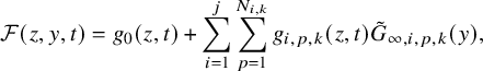 $$ \begin{align} \mathcal{F}(z,y,t)=g_{0}(z,t)+\sum_{i=1}^j\sum_{p=1}^{N_{i,k}}g_{i,p,k}(z,t)\tilde{G}_{\infty,i,p,k}(y), \end{align} $$
for some functions
 $g_0,g_{i,p,k}$
on
$g_0,g_{i,p,k}$
on
 $\mathbb {C}^m\times (-\infty ,0]$
. Since
$\mathbb {C}^m\times (-\infty ,0]$
. Since
 $\mathcal {F}$
is a polynomial in
$\mathcal {F}$
is a polynomial in
 $(z,t)$
of degree at most
$(z,t)$
of degree at most
 $2j$
, by fiberwise
$2j$
, by fiberwise
 $L^2$
projecting
$L^2$
projecting
 $\mathcal {F}$
onto each
$\mathcal {F}$
onto each
 $\tilde {G}_{\infty ,i,p,k}$
and onto the constants, we see that the coefficients
$\tilde {G}_{\infty ,i,p,k}$
and onto the constants, we see that the coefficients
 $g_0(z,t),g_{i,p,k}(z,t)$
are also polynomials of degree at most
$g_0(z,t),g_{i,p,k}(z,t)$
are also polynomials of degree at most
 $2j$
. This shows that
$2j$
. This shows that
 $\mathcal {F}$
is a linear combination of the functions
$\mathcal {F}$
is a linear combination of the functions
 $\tilde {G}_{\infty ,i,p,k}$
together with the constant
$\tilde {G}_{\infty ,i,p,k}$
together with the constant
 $1$
, with coefficients that are polynomials in
$1$
, with coefficients that are polynomials in
 $(z,t)$
of degree at most
$(z,t)$
of degree at most
 $2j$
, that is,
$2j$
, that is,
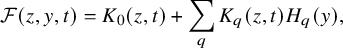 $$ \begin{align} \mathcal{F}(z,y,t)=K_0(z,t)+\sum_q K_q(z,t)H_q(y),\end{align} $$
where
 $K_0(z,t),K_q(z,t)$
are polynomials of degree at most
$K_0(z,t),K_q(z,t)$
are polynomials of degree at most
 $2j$
, and
$2j$
, and
 $H_q(y)$
are functions pulled back from the fiber Y that lie in
$H_q(y)$
are functions pulled back from the fiber Y that lie in
 $\mathcal {H}$
, the fiberwise span of the functions
$\mathcal {H}$
, the fiberwise span of the functions
 $\tilde {G}_{\infty ,i,p,k}, 1\leqslant i\leqslant j, 1\leqslant p\leqslant N_{i,k}$
.
$\tilde {G}_{\infty ,i,p,k}, 1\leqslant i\leqslant j, 1\leqslant p\leqslant N_{i,k}$
.
Following the argument in deriving [Reference Hein and Tosatti21, (4.330)] (which holds verbatim here), for each fixed
 $t\leqslant 0$
, we obtain
$t\leqslant 0$
, we obtain
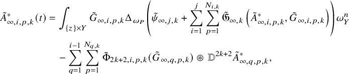 $$ \begin{align} \begin{aligned} \tilde A^{*}_{\infty,i,p,k}(t)&=\int_{\{z\}\times Y} \tilde G_{\infty,i,p,k} \Delta_{\omega_P} \left(\tilde \psi_{\infty,j,k}+\sum_{i=1}^j\sum_{p=1}^{N_{i,k}} \tilde{\mathfrak{G}}_{\infty,k}\left(\tilde A_{\infty,i,p,k}^{*},\tilde G_{\infty,i,p,k} \right) \right) \omega_Y^n\\ &\quad -\sum_{q=1}^{i-1}\sum_{p=1}^{N_{q,k}} \tilde \Phi_{2k+2,i,p,k}(\tilde G_{\infty,q,p,k}) \circledast \, {\mathbb{D}}^{2k+2}\tilde A_{\infty,q,p,k}^{*}, \end{aligned} \end{align} $$
where each quantity is evaluated at
 $t\leqslant 0$
. For notational convenience, we denote
$t\leqslant 0$
. For notational convenience, we denote
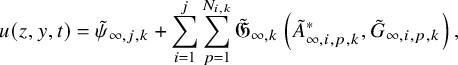 $$ \begin{align} u(z,y,t)=\tilde \psi_{\infty,j,k}+\sum_{i=1}^j\sum_{p=1}^{N_{i,k}} \tilde{\mathfrak{G}}_{\infty,k}\left( \tilde A_{\infty,i,p,k}^{*},\tilde G_{\infty,i,p,k} \right), \end{align} $$
which thanks to (4.366) satisfies
 $ \left(\partial _{t}-\Delta _{\omega _P}\right)u=\mathcal {F}$
, and so given any
$ \left(\partial _{t}-\Delta _{\omega _P}\right)u=\mathcal {F}$
, and so given any
 $p,q\geqslant 0$
with
$p,q\geqslant 0$
with
 $p+2q=2j+2$
, and given
$p+2q=2j+2$
, and given
 $v_1,\dots ,v_p$
tangent vectors to
$v_1,\dots ,v_p$
tangent vectors to
 $\mathbb {C}^m$
, from (4.369), we see that
$\mathbb {C}^m$
, from (4.369), we see that
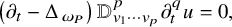 $$ \begin{align} \left(\partial_{t}-\Delta_{\omega_P}\right) {\mathbb{D}}^p_{v_1\cdots v_p}\partial_t^q u =0, \end{align} $$
while, thanks to (4.144), (4.145) and (4.185), we also have that
 ${\mathbb {D}}^p_{v_1\cdots v_p}\partial _t^q u=O(r^{\alpha })$
, where
${\mathbb {D}}^p_{v_1\cdots v_p}\partial _t^q u=O(r^{\alpha })$
, where
 $r=|z|+\sqrt {|t|}$
. Since
$r=|z|+\sqrt {|t|}$
. Since
 $\omega _P$
is of Ricci-flat, we can apply the Liouville Theorem in [Reference Fong and Lee11, Proposition 2.1] for ancient solutions of the heat equation, and conclude that
$\omega _P$
is of Ricci-flat, we can apply the Liouville Theorem in [Reference Fong and Lee11, Proposition 2.1] for ancient solutions of the heat equation, and conclude that
 ${\mathbb {D}}^p_{v_1\cdots v_p}\partial _t^q u$
is a constant in space and time. Since this is true for arbitrary
${\mathbb {D}}^p_{v_1\cdots v_p}\partial _t^q u$
is a constant in space and time. Since this is true for arbitrary
 $p,q$
with
$p,q$
with
 $p+2q=2j+2$
, and for arbitrary
$p+2q=2j+2$
, and for arbitrary
 $v_1,\dots ,v_p$
, this means that for every given
$v_1,\dots ,v_p$
, this means that for every given
 $y\in Y$
, the function
$y\in Y$
, the function
 $u(z,y,t)$
is a (parabolic) polynomial in
$u(z,y,t)$
is a (parabolic) polynomial in
 $(z,t)$
of degree at most
$(z,t)$
of degree at most
 $2j+2$
. Thus,
$2j+2$
. Thus,
 $(\partial _t u)(z,y,t)$
is a polynomial in
$(\partial _t u)(z,y,t)$
is a polynomial in
 $(z,t)$
of degree at most
$(z,t)$
of degree at most
 $2j$
; hence, the fiber integration
$2j$
; hence, the fiber integration
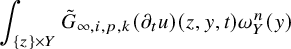 $$ \begin{align} \int_{\{z\}\times Y} \tilde G_{\infty,i,p,k} (\partial_t u)(z,y,t) \omega_Y^n(y) \end{align} $$
is also polynomial of degree at most
 $2j$
. Thus, if we insert (4.366) into (4.371), we obtain
$2j$
. Thus, if we insert (4.366) into (4.371), we obtain
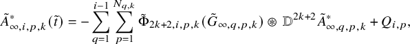 $$ \begin{align} \begin{aligned} \tilde A^{*}_{\infty,i,p,k}(\tilde t)&=-\sum_{q=1}^{i-1}\sum_{p=1}^{N_{q,k}} \tilde \Phi_{2k+2,i,p,k}(\tilde G_{\infty,q,p,k}) \circledast \, {\mathbb{D}}^{2k+2}\tilde A_{\infty,q,p,k}^{*}+Q_{i,p}, \end{aligned} \end{align} $$
where
 $Q_{i,p}$
is a (parabolic) polynomial on
$Q_{i,p}$
is a (parabolic) polynomial on
 $\mathbb {C}^m\times (-\infty ,0]$
of degree at most
$\mathbb {C}^m\times (-\infty ,0]$
of degree at most
 $2j$
. We can then use this to show by induction on
$2j$
. We can then use this to show by induction on
 $0\leqslant i\leqslant j$
that
$0\leqslant i\leqslant j$
that
 $\tilde {A}^{*}_{\infty ,i,p,k}=0$
for all
$\tilde {A}^{*}_{\infty ,i,p,k}=0$
for all
 $i,p$
. Indeed, in the base case of the induction
$i,p$
. Indeed, in the base case of the induction
 $i=1$
, the last term in (4.375) is not present, and so
$i=1$
, the last term in (4.375) is not present, and so
 $\tilde {A}^{*}_{\infty ,1,p,k}$
is a polynomial of degree at most
$\tilde {A}^{*}_{\infty ,1,p,k}$
is a polynomial of degree at most
 $2j$
, but since it also has vanishing
$2j$
, but since it also has vanishing
 $2j$
-jet at
$2j$
-jet at
 $(0,0)$
, it must be identically zero. The induction step is then exactly the same.
$(0,0)$
, it must be identically zero. The induction step is then exactly the same.
Next, since we have shown that
 $\tilde A_{\infty ,i,p,k}^{*}\equiv 0$
for all
$\tilde A_{\infty ,i,p,k}^{*}\equiv 0$
for all
 $i,p$
, from (4.357) and (4.372), we see that
$i,p$
, from (4.357) and (4.372), we see that
 $u=\tilde {\psi }_{\infty ,j,k}$
, which by (4.371) satisfies
$u=\tilde {\psi }_{\infty ,j,k}$
, which by (4.371) satisfies
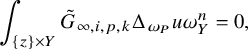 $$ \begin{align} \int_{\{z\}\times Y} \tilde G_{\infty,i,p,k} \Delta_{\omega_P}u\omega_Y^n=0, \end{align} $$
for all
 $z,i,p$
i.e., we have
$z,i,p$
i.e., we have
 $$ \begin{align} \Delta_{\omega_P} u \in \mathcal{H}^\perp, \end{align} $$
the fiberwise
 $L^2(\omega _Y)$
-orthogonal space to
$L^2(\omega _Y)$
-orthogonal space to
 $\mathcal {H}$
. Thanks to (4.366) and (4.369), we also have
$\mathcal {H}$
. Thanks to (4.366) and (4.369), we also have
 $$ \begin{align} \left(\partial_{t}-\Delta_{\omega_P}\right)u=\mathcal{F}\in \mathcal{H}. \end{align} $$
We then claim that we have
 $u\equiv 0$
. To show this, we apply a trick from [Reference Fong and Lee11, Claim 3.2]. We define a function v on
$u\equiv 0$
. To show this, we apply a trick from [Reference Fong and Lee11, Claim 3.2]. We define a function v on
 $\mathbb {C}^m\times Y\times (-\infty ,0]$
as the fiberwise
$\mathbb {C}^m\times Y\times (-\infty ,0]$
as the fiberwise
 $L^2(\omega _Y)$
-orthogonal projection of u onto
$L^2(\omega _Y)$
-orthogonal projection of u onto
 $\mathcal {H}^\perp $
. Recalling that
$\mathcal {H}^\perp $
. Recalling that
 $|u|=O(r^{2j+2+{\alpha }})$
, where
$|u|=O(r^{2j+2+{\alpha }})$
, where
 $r=|z|+\sqrt {|t|}$
, we claim that v satisfies the same growth bound
$r=|z|+\sqrt {|t|}$
, we claim that v satisfies the same growth bound
 $|v|=O(r^{2j+2+{\alpha }})$
. To see this, it suffices to prove this bound for the fiberwise
$|v|=O(r^{2j+2+{\alpha }})$
. To see this, it suffices to prove this bound for the fiberwise
 $L^2(\omega _Y)$
-orthogonal projection of u onto
$L^2(\omega _Y)$
-orthogonal projection of u onto
 $\mathcal {H}$
, which equals
$\mathcal {H}$
, which equals
 $$ \begin{align} \sum_{i=1}^j\sum_{p=1}^{N_{i,k}}\left(\int_{\{z\}\times Y} u(z,\cdot,t)\tilde{G}_{\infty,i,p,k}\omega_Y^n\right)\tilde{G}_{\infty,i,p,k}(y), \end{align} $$
and whose supremum on
 $B_r(0)\times (-r^2,0]$
is clearly bounded by
$B_r(0)\times (-r^2,0]$
is clearly bounded by
 $C\sup _{B_r(0)\times (-r^2,0]}|u|\leqslant Cr^{2j+2+{\alpha }},$
as claimed.
$C\sup _{B_r(0)\times (-r^2,0]}|u|\leqslant Cr^{2j+2+{\alpha }},$
as claimed.
Projecting (4.378) onto
 $\mathcal {H}^\perp $
, and using (4.377), we see that
$\mathcal {H}^\perp $
, and using (4.377), we see that
 $$ \begin{align} \partial_t v-\Delta_{\omega_P}u=0. \end{align} $$
Given
 $R>1$
, which later will be taken sufficiently large, we define a function on
$R>1$
, which later will be taken sufficiently large, we define a function on
 $\mathbb {C}^m\times Y\times (-\infty ,0]$
by
$\mathbb {C}^m\times Y\times (-\infty ,0]$
by
 $$ \begin{align} \phi_R(z,y,t):=e^{-\frac{|z|}{R}+\frac{t}{R}} \end{align} $$
and consider the weighted
 $L^2$
energy
$L^2$
energy
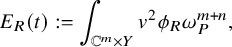 $$ \begin{align} E_R(t):=\int_{\mathbb{C}^m\times Y} v^2 \phi_R\omega_P^{m+n}, \end{align} $$
which is finite since
 $|v|=O(r^{2j+2+{\alpha }})$
and
$|v|=O(r^{2j+2+{\alpha }})$
and
 $\phi _R$
decays fast at spatial and time infinity. Differentiating
$\phi _R$
decays fast at spatial and time infinity. Differentiating
 $E_R$
in time and using (4.380), we get
$E_R$
in time and using (4.380), we get
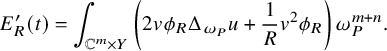 $$ \begin{align} \begin{aligned} E_R'(t)&=\int_{\mathbb{C}^m\times Y} \left( 2v\phi_R\Delta_{\omega_P} u +\frac1R v^2 \phi_R \right)\omega_P^{m+n}. \end{aligned} \end{align} $$
Since v is a fiberwise
 $L^2$
-projection of u, we have
$L^2$
-projection of u, we have
 $\int _Y v^2\omega _Y^n\leqslant \int _Yu^2\omega _Y^n$
. Using this, together with (4.377), we can estimate
$\int _Y v^2\omega _Y^n\leqslant \int _Yu^2\omega _Y^n$
. Using this, together with (4.377), we can estimate
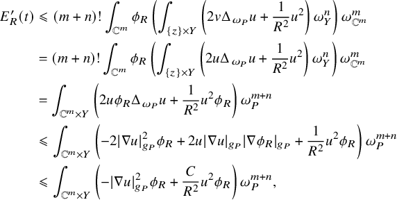 $$ \begin{align} \begin{aligned} E^{\prime}_R(t)&\leqslant (m+n)!\int_{\mathbb{C}^m}\phi_R \left( \int_{\{z\}\times Y}\left(2 v \Delta_{\omega_P}u+\frac{1}{R^2}u^2\right)\omega_Y^n \right)\omega_{\mathbb{C}^m}^m\\ &=(m+n)!\int_{\mathbb{C}^m}\phi_R \left( \int_{\{z\}\times Y}\left(2 u \Delta_{\omega_P}u+\frac{1}{R^2}u^2\right)\omega_Y^n \right)\omega_{\mathbb{C}^m}^m\\ &=\int_{\mathbb{C}^m\times Y} \left(2u\phi_R\Delta_{\omega_P} u +\frac{1}{R^2}u^2\phi_R\right)\omega_{P}^{m+n}\\ &\leqslant \int_{\mathbb{C}^m\times Y} \left( -2 |\nabla u|^2_{g_P} \phi_R +2u|\nabla u|_{g_P}|\nabla\phi_R|_{g_P}+\frac{1}{R^2} u^2 \phi_R \right)\omega_{P}^{m+n}\\ &\leqslant \int_{\mathbb{C}^m\times Y} \left( - |\nabla u|^2_{g_P} \phi_R +\frac{C}{R^2} u^2 \phi_R \right)\omega_{P}^{m+n}, \end{aligned} \end{align} $$
where the integration by part is justified by the growth bound of u and the fast decay of
 $\phi _R$
. Since u has fiberwise average zero, the Poincaré inequality on
$\phi _R$
. Since u has fiberwise average zero, the Poincaré inequality on
 $(Y,\omega _Y)$
implies
$(Y,\omega _Y)$
implies
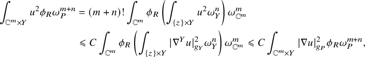 $$ \begin{align}\begin{aligned} \int_{\mathbb{C}^m\times Y} u^2 \phi_R \omega_P^{m+n}&=(m+n)!\int_{\mathbb{C}^m}\phi_R \left( \int_{\{z\}\times Y}u^2\omega_Y^n \right)\omega_{\mathbb{C}^m}^m\\ &\leqslant C\int_{\mathbb{C}^m}\phi_R \left( \int_{\{z\}\times Y}|\nabla^Y u|^2_{g_Y}\omega_Y^n \right)\omega_{\mathbb{C}^m}^m \leqslant C\int_{\mathbb{C}^m\times Y} |\nabla u|^2_{g_P} \phi_R \omega_P^{m+n}, \end{aligned}\end{align} $$
where the constant C is independent of R; hence, for all
 $t\leqslant 0$
, we have
$t\leqslant 0$
, we have
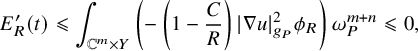 $$ \begin{align} E^{\prime}_R(t)\leqslant \int_{\mathbb{C}^m\times Y} \left( -\left(1-\frac{C}{R}\right) |\nabla u|^2_{g_P} \phi_R\right)\omega_{P}^{m+n}\leqslant 0, \end{align} $$
provided we choose R sufficiently large. Thus, for any
 $s<t\leqslant 0$
, we have
$s<t\leqslant 0$
, we have
 $E_R(t)\leqslant E_R(s)$
, but if we let
$E_R(t)\leqslant E_R(s)$
, but if we let
 $s\to -\infty $
, then since u grows at most polynomially while
$s\to -\infty $
, then since u grows at most polynomially while
 $\phi _R$
has exponential decay, we see that
$\phi _R$
has exponential decay, we see that
 $\lim _{s\to -\infty } E_R(s)=0$
, and so
$\lim _{s\to -\infty } E_R(s)=0$
, and so
 $E_R(t)\equiv 0$
for all
$E_R(t)\equiv 0$
for all
 $t\leqslant 0$
, which implies that
$t\leqslant 0$
, which implies that
 $v\equiv 0$
. From (4.378), we then see that
$v\equiv 0$
. From (4.378), we then see that
 $\Delta _{\omega _P}u\equiv 0$
, so u is harmonic on
$\Delta _{\omega _P}u\equiv 0$
, so u is harmonic on
 $\mathbb {C}^m\times Y$
and
$\mathbb {C}^m\times Y$
and
 $|u|=O(r^{2j+2+{\alpha }})$
, so [Reference Hein and Tosatti20, Proposition 3.12] implies that for any fixed
$|u|=O(r^{2j+2+{\alpha }})$
, so [Reference Hein and Tosatti20, Proposition 3.12] implies that for any fixed
 $t\leqslant 0$
, the function
$t\leqslant 0$
, the function
 $u(\cdot , t)$
is the pullback of a polynomial on
$u(\cdot , t)$
is the pullback of a polynomial on
 $\mathbb {C}^m$
of degree at most
$\mathbb {C}^m$
of degree at most
 $2j+2$
, and since it also has fiberwise average zero, it vanishes identically.
$2j+2$
, and since it also has fiberwise average zero, it vanishes identically.
To summarize, we have thus proved that
 $d_{\ell }^{-2j-{\alpha }}\tilde {\psi }_{\ell ,j,k}$
,
$d_{\ell }^{-2j-{\alpha }}\tilde {\psi }_{\ell ,j,k}$
,
 $d_{\ell }^{-2j-{\alpha }}\partial _{\tilde t}\underline{\tilde {\chi }_{\ell }^{*}}$
,
$d_{\ell }^{-2j-{\alpha }}\partial _{\tilde t}\underline{\tilde {\chi }_{\ell }^{*}}$
,
 $d_{\ell }^{-2j-{\alpha }}{i\partial \bar \partial }\underline{\tilde {\chi }_{\ell }^{*}},$
 $d_{\ell }^{-2j-{\alpha }}\tilde {A}^{*}_{\ell ,i,p,k}$
all go to zero locally uniformly in the appropriate topologies, which when
$d_{\ell }^{-2j-{\alpha }}\tilde {A}^{*}_{\ell ,i,p,k}$
all go to zero locally uniformly in the appropriate topologies, which when
 $j\geqslant 1$
shows that the RHS of (4.132) goes to zero, and gives a contradiction. As for the case
$j\geqslant 1$
shows that the RHS of (4.132) goes to zero, and gives a contradiction. As for the case
 $j=0$
, by definition, we have
$j=0$
, by definition, we have
 $$ \begin{align} {i\partial\bar\partial}\tilde{\varphi }_{\ell}={i\partial\bar\partial}\tilde{\psi}_{\ell,0,k}+e^{-d_{\ell}^2\lambda_{\ell}^{-2}\tilde{t}}{i\partial\bar\partial}\underline{\tilde{\chi}_{\ell}^{*}}+e^{-d_{\ell}^2\lambda_{\ell}^{-2}\tilde{t}}{i\partial\bar\partial}\underline{\tilde{\chi}_{\ell}^\sharp}, \end{align} $$
and we have just shown that
 $d_{\ell }^{-{\alpha }}{i\partial \bar \partial }\tilde {\psi }_{\ell ,0,k}$
and
$d_{\ell }^{-{\alpha }}{i\partial \bar \partial }\tilde {\psi }_{\ell ,0,k}$
and
 $d_{\ell }^{-{\alpha }}e^{-d_{\ell }^2\lambda _{\ell }^{-2}\tilde {t}}{i\partial \bar \partial }\underline{\tilde {\chi }_{\ell }^{*}}$
both go to zero locally uniformly, so using also (4.279), we see that the RHS of (4.110) also converges to zero, contradiction. This concludes Subcase B.
$d_{\ell }^{-{\alpha }}e^{-d_{\ell }^2\lambda _{\ell }^{-2}\tilde {t}}{i\partial \bar \partial }\underline{\tilde {\chi }_{\ell }^{*}}$
both go to zero locally uniformly, so using also (4.279), we see that the RHS of (4.110) also converges to zero, contradiction. This concludes Subcase B.
4.14 Subcase C:
$\varepsilon _{\ell }\to 0$

In this subcase, using repeatedly [Reference Hein and Tosatti21, Lemma 2.6], thanks to (4.144) and (4.145) we have that
 $d_{\ell }^{-2j-{\alpha }}\tilde {\psi }_{\ell ,j,k}$
converges to zero in
$d_{\ell }^{-2j-{\alpha }}\tilde {\psi }_{\ell ,j,k}$
converges to zero in
 $C^{2j+2+{\beta },j+1+{\beta }/2}_{\mathrm { loc}}$
. Also, using (4.194), we see that
$C^{2j+2+{\beta },j+1+{\beta }/2}_{\mathrm { loc}}$
. Also, using (4.194), we see that
 $d_{\ell }^{-2j-{\alpha }}\tilde {\eta }^\circ _{\ell ,j,k}$
converges in
$d_{\ell }^{-2j-{\alpha }}\tilde {\eta }^\circ _{\ell ,j,k}$
converges in
 $C^{2j+{\beta },j+{\beta }/2}_{\mathrm { loc}}$
to a
$C^{2j+{\beta },j+{\beta }/2}_{\mathrm { loc}}$
to a
 $(1,1)$
-form
$(1,1)$
-form
 $\tilde {\eta }^\circ _{\infty ,j,k}$
on
$\tilde {\eta }^\circ _{\infty ,j,k}$
on
 $\mathbb {C}^m\times Y\times (-\infty ,0]$
which is weakly closed. The bounds in (4.153) give us that
$\mathbb {C}^m\times Y\times (-\infty ,0]$
which is weakly closed. The bounds in (4.153) give us that
 $d_{\ell }^{-2j-{\alpha }}\partial _{\tilde t}\underline{\tilde {\chi }_{\ell }^{*}}$
and
$d_{\ell }^{-2j-{\alpha }}\partial _{\tilde t}\underline{\tilde {\chi }_{\ell }^{*}}$
and
 $d_{\ell }^{-2j-{\alpha }}{i\partial \bar \partial }\underline{\tilde {\chi }_{\ell }^{*}}$
converge in
$d_{\ell }^{-2j-{\alpha }}{i\partial \bar \partial }\underline{\tilde {\chi }_{\ell }^{*}}$
converge in
 $C_{\mathrm { loc}}^{2j+{\beta },j+{\beta }/2}$
for all
$C_{\mathrm { loc}}^{2j+{\beta },j+{\beta }/2}$
for all
 $0<{\beta }<{\alpha }$
to a function
$0<{\beta }<{\alpha }$
to a function
 $u_\infty \in C^{2j+{\alpha },j+{\alpha }/2}_{\mathrm {loc}}$
and to a
$u_\infty \in C^{2j+{\alpha },j+{\alpha }/2}_{\mathrm {loc}}$
and to a
 $(1,1)$
form
$(1,1)$
form
 $\eta _\infty \in C^{2j+{\alpha },j+{\alpha }/2}_{\mathrm {loc}}$
, respectively, on
$\eta _\infty \in C^{2j+{\alpha },j+{\alpha }/2}_{\mathrm {loc}}$
, respectively, on
 $\mathbb {C}^m\times (-\infty ,0]$
, and again
$\mathbb {C}^m\times (-\infty ,0]$
, and again
 $\eta _\infty $
is weakly closed, and these satisfy (4.356) when
$\eta _\infty $
is weakly closed, and these satisfy (4.356) when
 $j\geqslant 1$
. Using again (4.153), we also have that
$j\geqslant 1$
. Using again (4.153), we also have that
 $d_{\ell }^{-2j-{\alpha }}e^{-d_{\ell }^2\lambda _{\ell }^{-2}\tilde t}\partial _{\tilde t}\underline{\tilde \chi _{\ell }^{*} }\to u_\infty $
in
$d_{\ell }^{-2j-{\alpha }}e^{-d_{\ell }^2\lambda _{\ell }^{-2}\tilde t}\partial _{\tilde t}\underline{\tilde \chi _{\ell }^{*} }\to u_\infty $
in
 $C_{\mathrm {loc}}^{2j+{\beta },j+{\beta }/2}$
and
$C_{\mathrm {loc}}^{2j+{\beta },j+{\beta }/2}$
and
 $d_{\ell }^{-2j-{\alpha }}e^{-d_{\ell }^2\lambda _{\ell }^{-2}\tilde t}{i\partial \bar \partial }\underline{\tilde \chi _{\ell }^{*} }=d_{\ell }^{-2j-{\alpha }}\tilde {\eta }^\diamondsuit _{\ell }\to \eta _\infty $
in
$d_{\ell }^{-2j-{\alpha }}e^{-d_{\ell }^2\lambda _{\ell }^{-2}\tilde t}{i\partial \bar \partial }\underline{\tilde \chi _{\ell }^{*} }=d_{\ell }^{-2j-{\alpha }}\tilde {\eta }^\diamondsuit _{\ell }\to \eta _\infty $
in
 $C_{\mathrm {loc}}^{2j+{\beta },j+{\beta }/2}$
. From (4.160) and (4.203), we see that
$C_{\mathrm {loc}}^{2j+{\beta },j+{\beta }/2}$
. From (4.160) and (4.203), we see that
 $\tilde {\omega }^\sharp _{\ell }\to \omega _{\mathbb {C}^m}$
locally smoothly, and in particular, (as in [Reference Hein and Tosatti21, (4.345)]) this implies that
$\tilde {\omega }^\sharp _{\ell }\to \omega _{\mathbb {C}^m}$
locally smoothly, and in particular, (as in [Reference Hein and Tosatti21, (4.345)]) this implies that
 $$ \begin{align} d_{\ell}^{-2j-{\alpha}}\mathfrak{D}^{2j}_{\mathbf{bt}}\Delta_{\tilde{\omega}^\sharp_{\ell}}\underline{\tilde \chi_{\ell}^{*}}=d_{\ell}^{-2j-{\alpha}}\mathfrak{D}^{2j}_{\mathbf{bt}}\Delta_{\omega_{\mathbb{C}^m}}\underline{\tilde \chi_{\ell}^{*}}+o(1), \end{align} $$
locally uniformly, and so
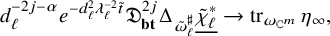 $$ \begin{align} d_{\ell}^{-2j-{\alpha}}e^{-d_{\ell}^2\lambda_{\ell}^{-2}\tilde t}\mathfrak{D}^{2j}_{\mathbf{bt}}\Delta_{\tilde{\omega}^\sharp_{\ell}}\underline{\tilde \chi_{\ell}^{*}}\to \operatorname{tr}_{\omega_{\mathbb{C}^m}}\eta_\infty, \end{align} $$
locally uniformly. Thanks to (4.170), we also have that for all
 $-1\leqslant \iota \leqslant 2k$
,
$-1\leqslant \iota \leqslant 2k$
,
 $$ \begin{align} \varepsilon_{\ell}^{\iota}d_{\ell}^{-2j-{\alpha}}\|\mathfrak{D}^{2j+2+\iota}\tilde{A}^{*}_{\ell, i,p,k}\|_{\infty, \tilde{Q}_R,\tilde{g}_{\ell}(0)}\to 0, \end{align} $$
so when
 $j=0$
, from (4.110) (using also (4.160)) we see that
$j=0$
, from (4.110) (using also (4.160)) we see that
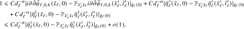 $$ \begin{align}\begin{aligned} 1&\leqslant Cd_{\ell}^{-\alpha}|{i\partial\bar\partial} \tilde{\psi}_{\ell,0,k}(\tilde x_{\ell},0)- \mathbb{P}_{\tilde x^{\prime}_{\ell}\tilde x_{\ell}}{i\partial\bar\partial}\tilde{\psi}_{\ell,0,k}(\tilde x^{\prime}_{\ell},\tilde t_{\ell}^{\prime})|_{\tilde g_{\ell}(0)} +Cd_{\ell}^{-\alpha}|\tilde{\eta}^\diamondsuit_{\ell}(\tilde x_{\ell},0)-\mathbb{P}_{\tilde x^{\prime}_{\ell}\tilde x_{\ell}}\tilde{\eta}^\diamondsuit_{\ell}(\tilde x^{\prime}_{\ell},\tilde t_{\ell}^{\prime})|_{\tilde g_{\ell}(0)}\\&\quad+Cd_{\ell}^{-\alpha}|\tilde{\eta}^\ddagger_{\ell}(\tilde x_{\ell},0)-\mathbb{P}_{\tilde x^{\prime}_{\ell}\tilde x_{\ell}}\tilde{\eta}^\ddagger_{\ell}(\tilde x^{\prime}_{\ell},\tilde t_{\ell}^{\prime})|_{\tilde g_{\ell}(0)}\\&\leqslant Cd_{\ell}^{-\alpha}|\tilde{\eta}^\diamondsuit_{\ell}(\tilde x_{\ell},0)-\mathbb{P}_{\tilde x^{\prime}_{\ell}\tilde x_{\ell}}\tilde{\eta}^\diamondsuit_{\ell}(\tilde x^{\prime}_{\ell},\tilde t_{\ell}^{\prime})|_{\tilde g_{\ell}(0)}+o(1), \end{aligned} \end{align} $$
while when
 $j\geqslant 1$
, from (4.132), we see that
$j\geqslant 1$
, from (4.132), we see that
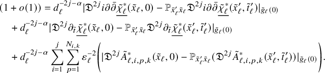 $$ \begin{align} \begin{aligned} & (1+o(1))=d_{\ell}^{-2j-{\alpha}}|\mathfrak{D}^{2j} {i\partial\bar\partial} \underline{\tilde{\chi}_{\ell}^{*}}(\tilde x_{\ell},0)- \mathbb{P}_{\tilde x^{\prime}_{\ell}\tilde x_{\ell}}\mathfrak{D}^{2j} {i\partial\bar\partial} \underline{\tilde{\chi}_{\ell}^{*}}(\tilde x^{\prime}_{\ell},\tilde t_{\ell}^{\prime})|_{\tilde g_{\ell}(0)}\\&\quad +d_{\ell}^{-2j-{\alpha}}|\mathfrak{D}^{2j} \partial_{\tilde t} \underline{\tilde{\chi}_{\ell}^{*}}(\tilde x_{\ell},0)- \mathbb{P}_{\tilde x^{\prime}_{\ell}\tilde x_{\ell}}\mathfrak{D}^{2j} \partial_{\tilde t} \underline{\tilde{\chi}_{\ell}^{*}}(\tilde x^{\prime}_{\ell},\tilde t_{\ell}^{\prime})|_{\tilde g_{\ell}(0)}\\&\quad +d_{\ell}^{-2j-{\alpha}}\sum_{i=1}^j \sum_{p=1}^{N_{i,k}}\varepsilon_{\ell}^{-2}\Bigg({|\mathfrak{D}^{2j} \tilde A^{*}_{\ell,i,p,k}(\tilde x_{\ell},0)- \mathbb{P}_{\tilde x_{\ell}^{\prime}\tilde x_{\ell}}(\mathfrak{D}^{2j}\tilde A^{*}_{\ell,i,p,k}(\tilde x_{\ell}^{\prime},\tilde t_{\ell}^{\prime}))|_{\tilde g_{\ell}(0)}}\Bigg). \end{aligned} \end{align} $$
We can then invoke (4.219), and use again the estimates (4.144) and (4.145), and see that
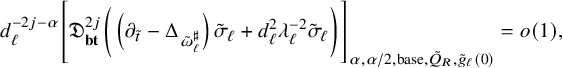 $$ \begin{align} d_{\ell}^{-2j-{\alpha}}\Bigg[ \mathfrak{D}^{2j}_{\textbf{bt}}\bigg(\left(\partial_{\tilde{t}}-\Delta_{\tilde \omega_{\ell}^\sharp}\right)\tilde{\sigma}_{\ell}+d_{\ell}^2\lambda_{\ell}^{-2}\tilde{\sigma}_{\ell} \bigg)\Bigg]_{{\alpha},{\alpha}/2,\mathrm{base},\tilde Q_R,\tilde g_{\ell}(0)}=o(1), \end{align} $$
where we have set
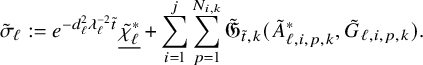 $$ \begin{align} \tilde{\sigma}_{\ell}:=e^{-d_{\ell}^2\lambda_{\ell}^{-2}\tilde t}\underline{\tilde{\chi}_{\ell}^{*}}+\sum_{i=1}^j\sum_{p=1}^{N_{i,k}} \tilde{\mathfrak{G}}_{\tilde{t},k}( \tilde A_{\ell,i,p,k}^{*},\tilde G_{\ell,i,p,k}). \end{align} $$
First, we dispose of the case
 $j=0$
. Again in this case from (4.268), we see that
$j=0$
. Again in this case from (4.268), we see that
 $u_\infty $
is a constant in space-time, hence identically zero, and as in subcase B, we see that
$u_\infty $
is a constant in space-time, hence identically zero, and as in subcase B, we see that
 $\eta _\infty $
is time-independent (using the argument in (4.364)). Then from (4.393), using also (4.157), we see that the quantity
$\eta _\infty $
is time-independent (using the argument in (4.364)). Then from (4.393), using also (4.157), we see that the quantity
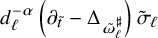 $$ \begin{align} d_{\ell}^{-{\alpha}}\left(\partial_{\tilde{t}}-\Delta_{\tilde \omega_{\ell}^\sharp}\right)\tilde{\sigma}_{\ell} \end{align} $$
is becoming asymptotically independent of the base and time directions, and so from (4.389), we conclude that
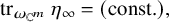 $$ \begin{align} \operatorname{tr}_{\omega_{\mathbb{C}^m}}\eta_\infty=(\mathrm{const.}), \end{align} $$
and since
 $\eta _\infty $
vanishes at
$\eta _\infty $
vanishes at
 $(0,0)$
, we actually have
$(0,0)$
, we actually have
 $\operatorname {tr}_{\omega _{\mathbb {C}^m}}\eta _\infty =0$
. As in Subcase B, we can write
$\operatorname {tr}_{\omega _{\mathbb {C}^m}}\eta _\infty =0$
. As in Subcase B, we can write
 $\eta _\infty ={i\partial \bar \partial } v_\infty $
, where
$\eta _\infty ={i\partial \bar \partial } v_\infty $
, where
 $v_\infty \in C^{2+{\alpha }}_{\mathrm {loc}}(\mathbb {C}^m)$
is time-independent and
$v_\infty \in C^{2+{\alpha }}_{\mathrm {loc}}(\mathbb {C}^m)$
is time-independent and
 $\Delta _{\omega _{\mathbb {C}^m}}v_\infty =0$
, so
$\Delta _{\omega _{\mathbb {C}^m}}v_\infty =0$
, so
 $v_\infty $
is smooth and
$v_\infty $
is smooth and
 $|{i\partial \bar \partial } v_\infty |=O(|z|^{\alpha })$
. The Liouville Theorem applied to each component of
$|{i\partial \bar \partial } v_\infty |=O(|z|^{\alpha })$
. The Liouville Theorem applied to each component of
 ${i\partial \bar \partial } v_\infty $
then implies that
${i\partial \bar \partial } v_\infty $
then implies that
 $\eta _\infty $
has constant coefficients; hence, it vanishes identically since its value at
$\eta _\infty $
has constant coefficients; hence, it vanishes identically since its value at
 $(0,0)$
vanishes. This means exactly that the RHS of (4.391) converges to zero, which gives us a contradiction when
$(0,0)$
vanishes. This means exactly that the RHS of (4.391) converges to zero, which gives us a contradiction when
 $j=0$
.
$j=0$
.
In the remainder of this section, we thus assume that
 $j\geqslant 1$
. Given any
$j\geqslant 1$
. Given any
 $p,q\geqslant 0$
with
$p,q\geqslant 0$
with
 $p+2q=2j+2$
, and given
$p+2q=2j+2$
, and given
 $v_1,\dots ,v_p$
tangent vectors to
$v_1,\dots ,v_p$
tangent vectors to
 $\mathbb {C}^m$
, from (4.393), recalling (4.157) and (4.181), we see that the quantity
$\mathbb {C}^m$
, from (4.393), recalling (4.157) and (4.181), we see that the quantity
 $$ \begin{align} d_{\ell}^{-2j-{\alpha}}{\mathbb{D}}^p_{v_1\cdots v_p}\partial_t^q\left(\partial_{\tilde{t}}-\Delta_{\tilde \omega_{\ell}^\sharp}\right)\left(e^{-d_{\ell}^2\lambda_{\ell}^{-2}\tilde t}\underline{\tilde{\chi}_{\ell}^{*}}+\sum_{i=1}^j\sum_{r=1}^{N_{i,k}} \tilde{\mathfrak{G}}_{\tilde{t},k}( \tilde A_{\ell,i,r,k}^{*},\tilde G_{\ell,i,r,k})\right) \end{align} $$
is asymptotically independent of the base and time directions. Recall then that from (4.193), we have
 $$ \begin{align} \begin{aligned} &\sum_{i=1}^j\sum_{r=1}^{N_{i,k}}d_{\ell}^{-2j-{\alpha}} {\mathbb{D}}^p_{v_1\cdots v_p}\partial_t^q \Delta_{\tilde \omega_{\ell}^\sharp}\tilde{\mathfrak{G}}_{\tilde{t},k}( \tilde A_{\ell,i,r,k}^{*},\tilde G_{\ell,i,r,k})\\[-2pt]&\quad= d_{\ell}^{-2j-{\alpha}} \sum_{i=1}^j \sum_{r=1}^{N_{i,k}} \operatorname{tr}_{\tilde{\omega}^\sharp_{\ell}}\left({i\partial\bar\partial} (\Delta_{\Theta_{\ell}^{*}\Psi_{\ell}^{*}\omega_{F}|_{ \{\cdot\}\times Y}})^{-1} \tilde G_{\ell,i,r,k} \right)_{\textbf{ff}}{\mathbb{D}}^p_{v_1\cdots v_p}\partial_t^q\tilde A_{\ell,i,r,k}^{*} +o(1)\\[-2pt]&\quad=d_{\ell}^{-2j-{\alpha}} \sum_{i=1}^j \sum_{r=1}^{N_{i,k}} \operatorname{tr}_{\varepsilon_{\ell}^2\Theta_{\ell}^{*}\Psi_{\ell}^{*}\omega_{F}}\left({i\partial\bar\partial} (\Delta_{\Theta_{\ell}^{*}\Psi_{\ell}^{*}\omega_{F}|_{ \{\cdot\}\times Y}})^{-1} \tilde G_{\ell,i,r,k} \right)_{\textbf{ff}}{\mathbb{D}}^p_{v_1\cdots v_p}\partial_t^q\tilde A_{\ell,i,r,k}^{*} +o(1)\\[-2pt]&\quad=\varepsilon_{\ell}^{-2}d_{\ell}^{-2j-{\alpha}} \sum_{i=1}^j \sum_{r=1}^{N_{i,k}} \tilde G_{\ell,i,r,k} {\mathbb{D}}^p_{v_1\cdots v_p}\partial_t^q\tilde A_{\ell,i,r,k}^{*} +o(1), \end{aligned} \end{align} $$
where in the second equality, we could exchange
 $\operatorname {tr}_{\tilde {\omega }^\sharp _{\ell }}({i\partial \bar \partial })_{\mathbf {ff}}$
with
$\operatorname {tr}_{\tilde {\omega }^\sharp _{\ell }}({i\partial \bar \partial })_{\mathbf {ff}}$
with
 $\operatorname {tr}_{\varepsilon _{\ell }^2\Theta _{\ell }^{*}\Psi _{\ell }^{*}\omega _{F}}({i\partial \bar \partial })_{\mathbf {ff}}$
with only a
$\operatorname {tr}_{\varepsilon _{\ell }^2\Theta _{\ell }^{*}\Psi _{\ell }^{*}\omega _{F}}({i\partial \bar \partial })_{\mathbf {ff}}$
with only a
 $o(1)$
error since
$o(1)$
error since
 $d_{\ell }^{-2j-{\alpha }}\|\mathfrak {D}^{2j}\tilde A_{\ell ,i,p,k}^{*}\|_{\infty ,\tilde {Q}_R,\tilde {g}_{\ell }(0)}\leqslant C\varepsilon _{\ell }^2$
by (4.170) and
$d_{\ell }^{-2j-{\alpha }}\|\mathfrak {D}^{2j}\tilde A_{\ell ,i,p,k}^{*}\|_{\infty ,\tilde {Q}_R,\tilde {g}_{\ell }(0)}\leqslant C\varepsilon _{\ell }^2$
by (4.170) and
 $\|\tilde {\eta }^\dagger _{\ell }\|_{\infty ,\tilde {Q}_R,\tilde {g}_{\ell }(0)}=o(1)$
by (4.200). Similarly, from (4.186), we see that
$\|\tilde {\eta }^\dagger _{\ell }\|_{\infty ,\tilde {Q}_R,\tilde {g}_{\ell }(0)}=o(1)$
by (4.200). Similarly, from (4.186), we see that
 $$ \begin{align} \begin{aligned} &d_{\ell}^{-2j-{\alpha}}{\mathbb{D}}^p_{v_1\cdots v_p}\partial_t^{q+1} \left( \sum_{i=1}^j\sum_{r=1}^{N_{i,k}} \tilde{\mathfrak{G}}_{\tilde{t},k}\left( \tilde A_{\ell,i,r,k}^{*},\tilde G_{\ell,i,r,k} \right)\right)\\&\quad=d_{\ell}^{-2j-{\alpha}}\sum_{i=1}^j\sum_{r=1}^{N_{i,k}} (\Delta_{\Theta_{\ell}^{*}\Psi_{\ell}^{*}\omega_{F}|_{ \{\cdot\}\times Y}})^{-1} \tilde G_{\ell,i,r,k}{\mathbb{D}}^p_{v_1\cdots v_p}\partial_t^{q+1} \tilde A_{\ell,i,r,k}^{*}+o(1), \end{aligned} \end{align} $$
while (4.388) implies that
 $$ \begin{align} d_{\ell}^{-2j-{\alpha}}{\mathbb{D}}^p_{v_1\cdots v_p}\partial_t^q\Delta_{\tilde \omega_{\ell}^\sharp}\left(e^{-d_{\ell}^2\lambda_{\ell}^{-2}\tilde t}\underline{\tilde{\chi}_{\ell}^{*}}\right) =d_{\ell}^{-2j-{\alpha}}{\mathbb{D}}^p_{v_1\cdots v_p}\partial_t^q\Delta_{\omega_{\mathbb{C}^m}}\left(e^{-d_{\ell}^2\lambda_{\ell}^{-2}\tilde t}\underline{\tilde{\chi}_{\ell}^{*}}\right)+o(1), \end{align} $$
and plugging (4.398), (4.399) and (4.400) into (4.397), we conclude that
 $$ \begin{align} \begin{aligned} &d_{\ell}^{-2j-{\alpha}}\left(\partial_{\tilde{t}}-\Delta_{\omega_{\mathbb{C}^m}}\right){\mathbb{D}}^p_{v_1\cdots v_p}\partial_t^q\left(e^{-d_{\ell}^2\lambda_{\ell}^{-2}\tilde t}\underline{\tilde{\chi}_{\ell}^{*}}\right)\\&\quad+d_{\ell}^{-2j-{\alpha}}\sum_{i=1}^j\sum_{r=1}^{N_{i,k}} \left( (\Delta_{\Theta_{\ell}^{*}\Psi_{\ell}^{*}\omega_{F}|_{ \{\cdot\}\times Y}})^{-1} \tilde G_{\ell,i,r,k}{\mathbb{D}}^p_{v_1\cdots v_p}\partial_t^{q+1} \tilde A_{\ell,i,r,k}^{*}-\varepsilon_{\ell}^{-2}\tilde G_{\ell,i,r,k} {\mathbb{D}}^p_{v_1\cdots v_p}\partial_t^q\tilde A_{\ell,i,r,k}^{*}\right) \end{aligned} \end{align} $$
is asymptotically independent of the base and time directions. Observe that the first line in (4.401) is a function pulled back from
 $\mathbb {C}^m$
, while the second line has fiberwise average zero. Thus, taking the fiberwise average of (4.401), we see that
$\mathbb {C}^m$
, while the second line has fiberwise average zero. Thus, taking the fiberwise average of (4.401), we see that
 $$ \begin{align} d_{\ell}^{-2j-{\alpha}}{\mathbb{D}}^p_{v_1\cdots v_p}\partial_t^q\left(\partial_{\tilde{t}}-\Delta_{\omega_{\mathbb{C}^m}}\right) \left(e^{-d_{\ell}^2\lambda_{\ell}^{-2}\tilde t}\underline{\tilde{\chi}_{\ell}^{*}}\right) \end{align} $$
is approaching a (time-independent) constant locally uniformly on
 $\mathbb {C}^m\times (-\infty ,0]$
. Recalling that
$\mathbb {C}^m\times (-\infty ,0]$
. Recalling that
 $d_{\ell }^{-2j-{\alpha }}\partial _{\tilde {t}}\left(e^{-d_{\ell }^2\lambda _{\ell }^{-2}\tilde t}\underline{\tilde {\chi }_{\ell }^{*}}\right)\to u_\infty $
in
$d_{\ell }^{-2j-{\alpha }}\partial _{\tilde {t}}\left(e^{-d_{\ell }^2\lambda _{\ell }^{-2}\tilde t}\underline{\tilde {\chi }_{\ell }^{*}}\right)\to u_\infty $
in
 $C^{2j+{\beta },j+{\beta }/2}_{\mathrm {loc}}$
and
$C^{2j+{\beta },j+{\beta }/2}_{\mathrm {loc}}$
and
 $d_{\ell }^{-2j-{\alpha }}\Delta _{\omega _{\mathbb {C}^m}}\left(e^{-d_{\ell }^2\lambda _{\ell }^{-2}\tilde t}\underline{\tilde {\chi }_{\ell }^{*}}\right)\to \operatorname {tr}_{\omega _{\mathbb {C}^m}}{\eta _\infty }$
in
$d_{\ell }^{-2j-{\alpha }}\Delta _{\omega _{\mathbb {C}^m}}\left(e^{-d_{\ell }^2\lambda _{\ell }^{-2}\tilde t}\underline{\tilde {\chi }_{\ell }^{*}}\right)\to \operatorname {tr}_{\omega _{\mathbb {C}^m}}{\eta _\infty }$
in
 $C^{2j+{\beta },j+{\beta }/2}_{\mathrm {loc}}$
, passing to the limit in (4.402) shows that
$C^{2j+{\beta },j+{\beta }/2}_{\mathrm {loc}}$
, passing to the limit in (4.402) shows that
 $u_\infty -\operatorname {tr}_{\omega _{\mathbb {C}^m}}{\eta _\infty }$
is a parabolic polynomial on
$u_\infty -\operatorname {tr}_{\omega _{\mathbb {C}^m}}{\eta _\infty }$
is a parabolic polynomial on
 $\mathbb {C}^m\times (-\infty ,0]$
of degree at most
$\mathbb {C}^m\times (-\infty ,0]$
of degree at most
 $2j$
, and since by jet subtraction the parabolic
$2j$
, and since by jet subtraction the parabolic
 $2j$
-jets of
$2j$
-jets of
 $u_\infty $
and
$u_\infty $
and
 $\eta _\infty $
vanish at
$\eta _\infty $
vanish at
 $(0,0)$
, we conclude that
$(0,0)$
, we conclude that
 $$ \begin{align} u_\infty-\operatorname{tr}_{\omega_{\mathbb{C}^m}}\eta_\infty=0, \end{align} $$
on
 $\mathbb {C}^m\times (-\infty ,0]$
. Since
$\mathbb {C}^m\times (-\infty ,0]$
. Since
 $j\geqslant 1$
, we can differentiate (4.403) with respect to t, and use (4.356) to see that
$j\geqslant 1$
, we can differentiate (4.403) with respect to t, and use (4.356) to see that
 $$ \begin{align} \begin{aligned} \partial_{\tilde t}u_\infty &=\operatorname{tr}_{\mathbb{C}^m}\partial_{\tilde t} \eta_\infty=\operatorname{tr}_{\mathbb{C}^m}{i\partial\bar\partial} u_\infty=\Delta_{\mathbb{C}^m}u_\infty, \end{aligned} \end{align} $$
so
 $u_\infty $
solves the heat equation on
$u_\infty $
solves the heat equation on
 $(-\infty ,0]\times \mathbb {C}^m$
, and
$(-\infty ,0]\times \mathbb {C}^m$
, and
 $|\mathfrak {D}^{\iota }u_\infty |=O(r^{2j+{\alpha }-\iota })$
for
$|\mathfrak {D}^{\iota }u_\infty |=O(r^{2j+{\alpha }-\iota })$
for
 $0\leqslant \iota \leqslant 2j$
by (4.153). By applying Liouville Theorem for ancient heat equation to
$0\leqslant \iota \leqslant 2j$
by (4.153). By applying Liouville Theorem for ancient heat equation to
 $\mathfrak {D}^{2j}u_\infty $
, we see that
$\mathfrak {D}^{2j}u_\infty $
, we see that
 $u_\infty $
must be a space-time polynomial of degree at most
$u_\infty $
must be a space-time polynomial of degree at most
 $2j$
, and hence,
$2j$
, and hence,
 $u_\infty \equiv 0$
since its parabolic
$u_\infty \equiv 0$
since its parabolic
 $2j$
-jet at
$2j$
-jet at
 $(0,0)$
vanishes. Going back to (4.356), it then follows that
$(0,0)$
vanishes. Going back to (4.356), it then follows that
 $\eta _\infty $
is time-independent, and it is clearly of the form
$\eta _\infty $
is time-independent, and it is clearly of the form
 $\eta _\infty ={i\partial \bar \partial } v_\infty $
for some time-independent function
$\eta _\infty ={i\partial \bar \partial } v_\infty $
for some time-independent function
 $v_\infty \in C^{2j+2+{\beta }}_{\mathrm {loc}}(\mathbb {C}^m)$
. From (4.403), we see that
$v_\infty \in C^{2j+2+{\beta }}_{\mathrm {loc}}(\mathbb {C}^m)$
. From (4.403), we see that
 $v_\infty $
is harmonic. Since
$v_\infty $
is harmonic. Since
 $|{\mathbb {D}}^{2j}\eta _\infty |=O(|z|^{\alpha })$
, the Liouville Theorem in [Reference Hein and Tosatti20, Proposition 3.12] then shows that the coefficients of
$|{\mathbb {D}}^{2j}\eta _\infty |=O(|z|^{\alpha })$
, the Liouville Theorem in [Reference Hein and Tosatti20, Proposition 3.12] then shows that the coefficients of
 $\eta _\infty $
are polynomials of degree at most
$\eta _\infty $
are polynomials of degree at most
 $2j$
, and since these coefficients have vanishing
$2j$
, and since these coefficients have vanishing
 $2j$
-jet at the origin, this implies that
$2j$
-jet at the origin, this implies that
 $\eta _\infty $
vanishes identically. This kills the first two terms on the RHS of (4.392).
$\eta _\infty $
vanishes identically. This kills the first two terms on the RHS of (4.392).
At this point, we return to (4.401), and subtracting its fiber average, we see that
 $$ \begin{align} d_{\ell}^{-2j-{\alpha}}\sum_{i=1}^j\sum_{r=1}^{N_{i,k}} \left( (\Delta_{\Theta_{\ell}^{*}\Psi_{\ell}^{*}\omega_{F}|_{ \{\cdot\}\times Y}})^{-1} \tilde G_{\ell,i,r,k}{\mathbb{D}}^p_{v_1\cdots v_p}\partial_t^{q+1} \tilde A_{\ell,i,r,k}^{*}-\varepsilon_{\ell}^{-2}\tilde G_{\ell,i,r,k} {\mathbb{D}}^p_{v_1\cdots v_p}\partial_t^q\tilde A_{\ell,i,r,k}^{*}\right) \end{align} $$
is asymptotically independent of the base and time directions. Let us then define a function
 $u_{\ell }$
on
$u_{\ell }$
on
 $\tilde {Q}_{Rd_{\ell }^{-1}}$
by
$\tilde {Q}_{Rd_{\ell }^{-1}}$
by
 $$ \begin{align} u_{\ell}(\tilde z,\tilde y,\tilde t):=d_{\ell}^{-2j-{\alpha}}\sum_{i=1}^j\sum_{r=1}^{N_{i,k}} (\Delta_{\Theta_{\ell}^{*}\Psi_{\ell}^{*}\omega_{F}|_{ \{\tilde z\}\times Y}})^{-1} \tilde G_{\ell,i,r,k} {\mathbb{D}}^p_{v_1\cdots v_p}\partial_t^q\tilde A_{\ell,i,r,k}^{*}, \end{align} $$
so that (4.405) is equivalent to the statement that
 $$ \begin{align} (\partial_{\tilde t}-\Delta_{\varepsilon_{\ell}^2\Theta_{\ell}^{*}\Psi_{\ell}^{*} \omega_{F}|_{ \{\cdot\}\times Y}}) u_{\ell} \end{align} $$
is asymptotically independent of the base and time directions.
Our next goal is to show that
 $u_{\ell }$
itself is asymptotically constant in the base and time directions. Fix any two points
$u_{\ell }$
itself is asymptotically constant in the base and time directions. Fix any two points
 $z,z'\in \mathbb {C}^m$
and times
$z,z'\in \mathbb {C}^m$
and times
 $t,t'\in (-\infty ,0]$
and consider
$t,t'\in (-\infty ,0]$
and consider
 $$ \begin{align} v_{\ell}(\tilde y,\tilde t)=u_{\ell}( z,\tilde y,t+\tilde t)-u_{\ell}( z',\tilde y,t'+\tilde t), \end{align} $$
so that in
 $L^\infty _{\mathrm {loc}}(Y)$
, we have
$L^\infty _{\mathrm {loc}}(Y)$
, we have
 $$ \begin{align} \begin{aligned} &\left((\partial_{\tilde t}-\Delta_{\varepsilon_{\ell}^2\Theta_{\ell}^{*}\Psi_{\ell}^{*} \omega_{F}|_{ \{z\}\times Y}}) v_{\ell}\right)(\tilde{y},0)\\&\quad=\left((\partial_{\tilde t}-\Delta_{\varepsilon_{\ell}^2\Theta_{\ell}^{*}\Psi_{\ell}^{*} \omega_{F}|_{ \{z\}\times Y}})u_{\ell}\right)( z,\tilde y,t)-\left((\partial_{\tilde t}-\Delta_{\varepsilon_{\ell}^2\Theta_{\ell}^{*}\Psi_{\ell}^{*} \omega_{F}|_{ \{z\}\times Y}}) u_{\ell}\right)( z',\tilde y,t')\\&\quad=\left( \Delta_{\varepsilon_{\ell}^2\Theta_{\ell}^{*}\Psi_{\ell}^{*}\omega_F|_{ \{z\}\times Y}}-\Delta_{\varepsilon_{\ell}^2\Theta_{\ell}^{*}\Psi_{\ell}^{*}\omega_F|_{ \{z'\}\times Y}}\right) u_{\ell}( z',\tilde y,t')+o(1), \end{aligned} \end{align} $$
and we can schematically estimate the difference of Laplacians by
 $$ \begin{align} \varepsilon_{\ell}^{-2}\left(g_F^{\mathbf{ff}}(d_{\ell}\lambda_{\ell}^{-1}z,\tilde{y})-g_F^{\mathbf{ff}}(d_{\ell}\lambda_{\ell}^{-1}z',\tilde{y})\right)({i\partial\bar\partial} u_{\ell})_{\mathbf{ff}}(z',\tilde{y},t'), \end{align} $$
and since
 $$ \begin{align} ({i\partial\bar\partial} u_{\ell})_{\mathbf{ff}}(z',\tilde{y},t')=d_{\ell}^{-2j-{\alpha}}\sum_{i=1}^j\sum_{r=1}^{N_{i,k}} \left({i\partial\bar\partial}(\Delta_{\Theta_{\ell}^{*}\Psi_{\ell}^{*}\omega_{F}|_{ \{z'\}\times Y}})^{-1} \tilde G_{\ell,i,r,k}\right)_{\mathbf{ff}} {\mathbb{D}}^p_{v_1\cdots v_p}\partial_t^q\tilde A_{\ell,i,r,k}^{*}, \end{align} $$
we can use (4.163) with
 $\iota =2j$
to estimate
$\iota =2j$
to estimate
 $|({i\partial \bar \partial } u_{\ell })_{\mathbf {ff}}|\leqslant C\varepsilon _{\ell }^2$
, and so (4.410) can be estimated by
$|({i\partial \bar \partial } u_{\ell })_{\mathbf {ff}}|\leqslant C\varepsilon _{\ell }^2$
, and so (4.410) can be estimated by
 $$ \begin{align} C\left|g_F^{\mathbf{ff}}(d_{\ell}\lambda_{\ell}^{-1}z,\tilde{y})-g_F^{\mathbf{ff}}(d_{\ell}\lambda_{\ell}^{-1}z',\tilde{y})\right|\leqslant Cd_{\ell}\lambda_{\ell}^{-1}|z-z'|=o(1), \end{align} $$
so that (4.409) shows that
 $$ \begin{align} (\partial_{\tilde t}-\Delta_{\varepsilon_{\ell}^2\Theta_{\ell}^{*}\Psi_{\ell}^{*}\omega_F|_{ \{z\}\times Y}}) v_{\ell}=o(1), \end{align} $$
locally uniformly. So the functions
 $v_{\ell }$
are approximate solutions of a fiberwise heat equation, with time parameter
$v_{\ell }$
are approximate solutions of a fiberwise heat equation, with time parameter
 $\tilde {t}\in (-\infty ,0]$
. We then employ another energy argument on the given fiber
$\tilde {t}\in (-\infty ,0]$
. We then employ another energy argument on the given fiber
 $\{z\}\times Y$
. First, observe that (4.163) with
$\{z\}\times Y$
. First, observe that (4.163) with
 $\iota =2j$
implies
$\iota =2j$
implies
 $$ \begin{align} |\varepsilon_{\ell}^{-2}v_{\ell}|\leqslant C. \end{align} $$
For notational convenience, we denote by
 $\omega _Y:=\Theta _{\ell }^{*}\Psi _{\ell }^{*}\omega _F|_{\{z\}\times Y}$
and consider then the energy
$\omega _Y:=\Theta _{\ell }^{*}\Psi _{\ell }^{*}\omega _F|_{\{z\}\times Y}$
and consider then the energy
 $$ \begin{align} E_{\ell}(\tilde{t})=\varepsilon_{\ell}^{-4}\int_Y v_{\ell}^2\, \omega_Y^n, \end{align} $$
which satisfies
 $E_{\ell }(\tilde {t})\leqslant C$
for all
$E_{\ell }(\tilde {t})\leqslant C$
for all
 $\tilde {t}\leqslant 0$
, and denote by
$\tilde {t}\leqslant 0$
, and denote by
 $$ \begin{align} \sigma_{\ell}:=\left\|\left(\partial_{\tilde{t}}-\Delta_{\varepsilon_{\ell}^2\omega_Y}\right) v_{\ell}\right\|_{\infty, \tilde Q_{2R}}, \end{align} $$
where
 $R>0$
is fixed so that
$R>0$
is fixed so that
 $(z,t),(z',t')\in Q_{2R}$
. Thanks to (4.413), we have
$(z,t),(z',t')\in Q_{2R}$
. Thanks to (4.413), we have
 $\sigma _{\ell }\to 0$
. We can then compute, using the Poincaré inequality on
$\sigma _{\ell }\to 0$
. We can then compute, using the Poincaré inequality on
 $(Y,\omega _Y)$
(recall that
$(Y,\omega _Y)$
(recall that
 $v_{\ell }$
has fiberwise average zero),
$v_{\ell }$
has fiberwise average zero),
 $$ \begin{align} \begin{aligned} \frac{d}{d\tilde{t}} E_{\ell}&=-2\varepsilon_{\ell}^{-6}\int_Y |\nabla^Y v_{\ell}|^2_{g_Y}\, \omega_Y^n+2\varepsilon_{\ell}^{-4}\int_Y v_{\ell} \left(\partial_t-\Delta_{\varepsilon_{\ell}^2\omega_Y}\right) v_{\ell} \, \omega_Y^n\\\ &\leqslant -2C^{-1} \varepsilon_{\ell}^{-2} E_{\ell}(\tilde{t})+2\sigma_{\ell}\varepsilon_{\ell}^{-4}\int_Y v_{\ell} \omega_Y^n\\ &\leqslant -2C^{-1} \varepsilon_{\ell}^{-2} E_{\ell}(\tilde{t})+C\sigma_{\ell} \varepsilon_{\ell}^{-2} E_{\ell}(\tilde{t})^{\frac{1}{2}}, \end{aligned} \end{align} $$
and using the Young inequality
 $\sigma _{\ell } E_{\ell }(\tilde {t})^{\frac {1}{2}}\leqslant C^{-1}E_{\ell }(\tilde {t})+C\sigma _{\ell }^2,$
we can bound
$\sigma _{\ell } E_{\ell }(\tilde {t})^{\frac {1}{2}}\leqslant C^{-1}E_{\ell }(\tilde {t})+C\sigma _{\ell }^2,$
we can bound
 $$ \begin{align} \frac{d}{d\tilde{t}} E_{\ell}\leqslant -C^{-1} \varepsilon_{\ell}^{-2} E_{\ell}+C\sigma_{\ell}^2 \varepsilon_{\ell}^{-2}. \end{align} $$
We will compare
 $E_{\ell }$
with the real-variable function
$E_{\ell }$
with the real-variable function
 $F_{\ell }$
which solves the ODE
$F_{\ell }$
which solves the ODE
 $$ \begin{align} F^{\prime}_{\ell}=-C^{-1} \varepsilon_{\ell}^{-2} F_{\ell}+C\sigma_{\ell}^2 \varepsilon_{\ell}^{-2},\quad F^{\prime}_{\ell}(-R^2)=A, \end{align} $$
which is given explicitly by
 $$ \begin{align} F_{\ell}(\tilde{t})=Ae^{-C^{-1}\varepsilon_{\ell}^{-2}(R^2+\tilde{t})}+C^2\sigma_{\ell}^2\left(1-e^{-C^{-1}\varepsilon_{\ell}^{-2}(R^2+\tilde{t})}\right), \end{align} $$
and if we choose A large enough so that
 $E_{\ell }(\tilde {t})\leqslant A$
for all
$E_{\ell }(\tilde {t})\leqslant A$
for all
 $\tilde {t}\leqslant 0$
(which is possible, as shown above), then we conclude that for all
$\tilde {t}\leqslant 0$
(which is possible, as shown above), then we conclude that for all
 $\tilde {t}\in [-R^2,0]$
, we have
$\tilde {t}\in [-R^2,0]$
, we have
 $$ \begin{align} E_{\ell}(\tilde{t})\leqslant F_{\ell}(\tilde{t})=Ae^{-C^{-1}\varepsilon_{\ell}^{-2}(R^2+\tilde{t})}+C^2\sigma_{\ell}^2\left(1-e^{-C^{-1}\varepsilon_{\ell}^{-2}(R^2+\tilde{t})}\right), \end{align} $$
and hence in particular
 $E_{\ell }(0)\to 0$
as
$E_{\ell }(0)\to 0$
as
 $\ell \to +\infty $
. This means that the functions
$\ell \to +\infty $
. This means that the functions
 $\varepsilon _{\ell }^{-2}v_{\ell }(\cdot , 0)$
, which are defined on Y and are uniformly bounded by (4.414), converge to
$\varepsilon _{\ell }^{-2}v_{\ell }(\cdot , 0)$
, which are defined on Y and are uniformly bounded by (4.414), converge to
 $0$
in
$0$
in
 $L^2(Y,\omega _Y^n)$
. Recalling the definitions (4.406), (4.408), this means that the function of
$L^2(Y,\omega _Y^n)$
. Recalling the definitions (4.406), (4.408), this means that the function of
 $\tilde {y}$
given by
$\tilde {y}$
given by
 $$ \begin{align} \begin{aligned} &d_{\ell}^{-2j-{\alpha}}\varepsilon_{\ell}^{-2}\sum_{i=1}^j\sum_{r=1}^{N_{i,k}} ((\Delta_{\Theta_{\ell}^{*}\Psi_{\ell}^{*}\omega_{F}|_{ \{z\}\times Y}})^{-1} \tilde G_{\ell,i,r,k})(z,\tilde{y}) ({\mathbb{D}}^p_{v_1\cdots v_p}\partial_t^q\tilde A_{\ell,i,r,k}^{*})(z,t)\\&\quad -d_{\ell}^{-2j-{\alpha}}\varepsilon_{\ell}^{-2}\sum_{i=1}^j\sum_{r=1}^{N_{i,k}} ((\Delta_{\Theta_{\ell}^{*}\Psi_{\ell}^{*}\omega_{F}|_{ \{z'\}\times Y}})^{-1} \tilde G_{\ell,i,r,k})(z',\tilde{y}) ({\mathbb{D}}^p_{v_1\cdots v_p}\partial_t^q\tilde A_{\ell,i,r,k}^{*})(z',t') \end{aligned} \end{align} $$
converges to zero in
 $L^2(Y,\omega _Y^n)$
. However, we have
$L^2(Y,\omega _Y^n)$
. However, we have
 $$ \begin{align} \begin{aligned} ((\Delta_{\Theta_{\ell}^{*}\Psi_{\ell}^{*}\omega_{F}|_{ \{z'\}\times Y}})^{-1} \tilde G_{\ell,i,r,k})(z',\tilde{y})&= ((\Delta_{\omega_{F}|_{ \{d_{\ell}\lambda_{\ell}^{-1}z'\}\times Y}})^{-1} G_{\ell,i,r,k})(d_{\ell}\lambda_{\ell}^{-1}z',\tilde{y})\\ &=((\Delta_{\omega_{F}|_{ \{d_{\ell}\lambda_{\ell}^{-1}z\}\times Y}})^{-1} G_{\ell,i,r,k})(d_{\ell}\lambda_{\ell}^{-1}z,\tilde{y})+O(d_{\ell}\lambda_{\ell}^{-1})\\ &=((\Delta_{\Theta_{\ell}^{*}\Psi_{\ell}^{*}\omega_{F}|_{ \{z\}\times Y}})^{-1} \tilde G_{\ell,i,r,k})(z,\tilde{y})+O(d_{\ell}\lambda_{\ell}^{-1}), \end{aligned} \end{align} $$
where in the second equality we used that since
 $G_{\ell ,i,r,k}$
is a smooth function on the total space with fiberwise average zero, the function
$G_{\ell ,i,r,k}$
is a smooth function on the total space with fiberwise average zero, the function
 $(\Delta _{\omega _{F}|_{ \{\cdot \}\times Y}})^{-1}G_{\ell ,i,r,k}$
is also smooth on the total space (by standard Schauder theory fiber-by-fiber, with continuous dependence on the base variables). Using (4.423) together with the bound
$(\Delta _{\omega _{F}|_{ \{\cdot \}\times Y}})^{-1}G_{\ell ,i,r,k}$
is also smooth on the total space (by standard Schauder theory fiber-by-fiber, with continuous dependence on the base variables). Using (4.423) together with the bound
 $d_{\ell }^{-2j-{\alpha }}\varepsilon _{\ell }^{-2}|{\mathbb {D}}^p_{v_1\cdots v_p}\partial _t^q\tilde A_{\ell ,i,r,k}^{*}|\leqslant C$
, which comes from (4.163) with
$d_{\ell }^{-2j-{\alpha }}\varepsilon _{\ell }^{-2}|{\mathbb {D}}^p_{v_1\cdots v_p}\partial _t^q\tilde A_{\ell ,i,r,k}^{*}|\leqslant C$
, which comes from (4.163) with
 $\iota =2j$
, we see that
$\iota =2j$
, we see that
 $$ \begin{align} \begin{aligned} &d_{\ell}^{-2j-{\alpha}}\varepsilon_{\ell}^{-2}\sum_{i=1}^j\sum_{r=1}^{N_{i,k}} ((\Delta_{\Theta_{\ell}^{*}\Psi_{\ell}^{*}\omega_{F}|_{ \{z'\}\times Y}})^{-1} \tilde G_{\ell,i,r,k})(z',\tilde{y}) ({\mathbb{D}}^p_{v_1\cdots v_p}\partial_t^q\tilde A_{\ell,i,r,k}^{*})(z',t')\\&\quad =d_{\ell}^{-2j-{\alpha}}\varepsilon_{\ell}^{-2}\sum_{i=1}^j\sum_{r=1}^{N_{i,k}} ((\Delta_{\Theta_{\ell}^{*}\Psi_{\ell}^{*}\omega_{F}|_{ \{z\}\times Y}})^{-1} \tilde G_{\ell,i,r,k})(z,\tilde{y}) ({\mathbb{D}}^p_{v_1\cdots v_p}\partial_t^q\tilde A_{\ell,i,r,k}^{*})(z',t')+o(1), \end{aligned} \end{align} $$
so from (4.422), we see that
 $$ \begin{align} d_{\ell}^{-2j-{\alpha}}\varepsilon_{\ell}^{-2}\sum_{i=1}^j\sum_{r=1}^{N_{i,k}} ((\Delta_{\Theta_{\ell}^{*}\Psi_{\ell}^{*}\omega_{F}|_{ \{z\}\times Y}})^{-1} \tilde G_{\ell,i,r,k})(z,\tilde{y}) \left(({\mathbb{D}}^p_{v_1\cdots v_p}\partial_t^q\tilde A_{\ell,i,r,k}^{*})(z,t)-({\mathbb{D}}^p_{v_1\cdots v_p}\partial_t^q\tilde A_{\ell,i,r,k}^{*})(z',t')\right) \end{align} $$
also converges to zero in
 $L^2(Y,\omega _Y^n)$
. Now, the functions
$L^2(Y,\omega _Y^n)$
. Now, the functions
 $\{(\Delta _{\Theta _{\ell }^{*}\Psi _{\ell }^{*}\omega _{F}|_{ \{z\}\times Y}})^{-1} \tilde G_{\ell ,i,r,k}\}_{i,r}$
are fiberwise linearly independent (since so are
$\{(\Delta _{\Theta _{\ell }^{*}\Psi _{\ell }^{*}\omega _{F}|_{ \{z\}\times Y}})^{-1} \tilde G_{\ell ,i,r,k}\}_{i,r}$
are fiberwise linearly independent (since so are
 $\{\tilde G_{\ell ,i,r,k}\}_{i,r}$
), and the function in (4.425) along the fiber
$\{\tilde G_{\ell ,i,r,k}\}_{i,r}$
), and the function in (4.425) along the fiber
 $\{z\}\times Y$
is expressed as a linear combination of these functions with coefficients (which are constants on Y) given by
$\{z\}\times Y$
is expressed as a linear combination of these functions with coefficients (which are constants on Y) given by
 $$ \begin{align} d_{\ell}^{-2j-{\alpha}}\varepsilon_{\ell}^{-2}\left(({\mathbb{D}}^p_{v_1\cdots v_p}\partial_t^q\tilde A_{\ell,i,r,k}^{*})(z,t)-({\mathbb{D}}^p_{v_1\cdots v_p}\partial_t^q\tilde A_{\ell,i,r,k}^{*})(z',t')\right). \end{align} $$
Since the
 $L^2$
norm of (4.425) is going to zero, these coefficients must be going to zero too, which means that the functions
$L^2$
norm of (4.425) is going to zero, these coefficients must be going to zero too, which means that the functions
 $$ \begin{align} d_{\ell}^{-2j-{\alpha}}\varepsilon_{\ell}^{-2}{\mathbb{D}}^p_{v_1\cdots v_p}\partial_t^q\tilde A_{\ell,i,r,k}^{*} \end{align} $$
are approximately constant (in space and time) as
 $\ell \to +\infty $
. This kills the last term on the RHS of (4.392) and gives the final contradiction, thus completing the proof of Subcase C and of Theorem 4.2.
$\ell \to +\infty $
. This kills the last term on the RHS of (4.392) and gives the final contradiction, thus completing the proof of Subcase C and of Theorem 4.2.
5 Proof of the main theorem
In this final section, we give the proof of our main Theorem 1.3; namely, we prove Conjectures 1.1 and 1.2. The asymptotic expansion in Theorem 4.2 will play a crucial role.
5.1 Higher order estimates
To prove the higher order estimates in Conjecture 1.1 from the expansion in Theorem 4.2, we follow the arguments in [Reference Hein and Tosatti21, Proof of Theorem A], but since our estimate (4.16) is weaker than the corresponding [Reference Hein and Tosatti21, (4.12)], we will have to deal with some new difficulties. As explained in the Introduction, in this section we work locally on the base (away from the image of the singular fibers), and the Kähler-Ricci flow that we analyze thus lives on
 $B\times Y\times [0,+\infty )$
(with a non-product complex structure) for some Euclidean ball
$B\times Y\times [0,+\infty )$
(with a non-product complex structure) for some Euclidean ball
 $B\subset \mathbb {C}^m$
. For brevity, in this section, all norms and seminorms will be tacitly taken on
$B\subset \mathbb {C}^m$
. For brevity, in this section, all norms and seminorms will be tacitly taken on
 $B\times Y\times [t-1,t]$
(or
$B\times Y\times [t-1,t]$
(or
 $B\times [t-1,t]$
for objects that live on the base), without making this explicit in the notation. The ball B and the interval
$B\times [t-1,t]$
for objects that live on the base), without making this explicit in the notation. The ball B and the interval
 $[t-1,t]$
will also be shrunk slightly every time we use interpolation.
$[t-1,t]$
will also be shrunk slightly every time we use interpolation.
Given an even integer
 $k\geqslant 2$
, we want to show that
$k\geqslant 2$
, we want to show that
 $\omega ^{\bullet }(t)$
is uniformly bounded in
$\omega ^{\bullet }(t)$
is uniformly bounded in
 $C^k(g_X)$
. Applying Theorem 4.2 with
$C^k(g_X)$
. Applying Theorem 4.2 with
 $j:=\frac {k}{2}$
, up to shrinking B, we can write
$j:=\frac {k}{2}$
, up to shrinking B, we can write
 $$ \begin{align} \omega^{\bullet}(t)=\omega^\natural(t)+\gamma_0(t)+\gamma_{1,k}(t)+\cdots+\gamma_{\frac{k}{2},k}(t)+\eta_{\frac{k}{2},k}(t), \end{align} $$
and in this decomposition,
 $\omega ^\natural (t)$
is clearly bounded in
$\omega ^\natural (t)$
is clearly bounded in
 $C^k(g_X)$
,
$C^k(g_X)$
,
 $\gamma _0(t)$
has a similar bound by (4.12),
$\gamma _0(t)$
has a similar bound by (4.12),
 $\eta _{\frac {k}{2},k}(t)$
is bounded in the shrinking
$\eta _{\frac {k}{2},k}(t)$
is bounded in the shrinking
 $C^k$
norm by (4.9) (hence in the regular
$C^k$
norm by (4.9) (hence in the regular
 $C^k(g_X)$
norm by [Reference Hein and Tosatti21, Lemma 2.6]), so we are left with dealing with the terms
$C^k(g_X)$
norm by [Reference Hein and Tosatti21, Lemma 2.6]), so we are left with dealing with the terms
 $\gamma _{i,k}(t),1\leqslant i\leqslant \frac {k}{2}$
. By definition and using (3.1), we have
$\gamma _{i,k}(t),1\leqslant i\leqslant \frac {k}{2}$
. By definition and using (3.1), we have
 $$ \begin{align} \gamma_{i,k}(t)={i\partial\bar\partial}\sum_{p=1}^{N_{i,k}}\sum_{\iota=0}^{2k}\sum_{r=\lceil\frac{\iota}{2}\rceil}^{k}e^{-r t}\Phi_{\iota,r}(G_{i,p,k})\circledast{\mathbb{D}}^\iota A_{i,p,k}(t), \end{align} $$
and so, as in [Reference Hein and Tosatti21, (5.10)], for
 $0\leqslant q\leqslant k$
,
$0\leqslant q\leqslant k$
,
 $$ \begin{align} \mathfrak{D}^q\gamma_{i,k}=\sum_{p=1}^{N_{i,k}}\sum_{\iota=0}^{2k}\sum_{r=\lceil\frac{\iota}{2}\rceil}^{k}\sum_{s=0}^{q+1}\sum_{i_1+i_2=s+1}e^{-r t}({\mathbb{D}}^{q+1-s}J)\circledast{\mathbb{D}}^{i_1}\Phi_{\iota,r}(G_{i,p,k})\circledast\mathfrak{D}^{i_2+\iota} A_{i,p,k}, \end{align} $$
and using the fixed metric
 $g_X$
, we can estimate
$g_X$
, we can estimate
 $|{\mathbb {D}}^{i_1}\Phi _{\iota ,r}(G_{i,p,k})|_{g_X}\leqslant C$
and
$|{\mathbb {D}}^{i_1}\Phi _{\iota ,r}(G_{i,p,k})|_{g_X}\leqslant C$
and
 $|({\mathbb {D}}^{q+1-s}J)|_{g_X}\leqslant C$
, while from (4.16), we see that
$|({\mathbb {D}}^{q+1-s}J)|_{g_X}\leqslant C$
, while from (4.16), we see that
 $|\mathfrak {D}^{i_2+\iota } A_{i,p,k}|=o(1)$
when
$|\mathfrak {D}^{i_2+\iota } A_{i,p,k}|=o(1)$
when
 $i_2+\iota \leqslant k+2$
and from (4.17) that
$i_2+\iota \leqslant k+2$
and from (4.17) that
 $|\mathfrak {D}^{i_2+\iota } A_{i,p,k}|=o(e^{(i_2+\iota -k-2)\frac {t}{2}})$
when
$|\mathfrak {D}^{i_2+\iota } A_{i,p,k}|=o(e^{(i_2+\iota -k-2)\frac {t}{2}})$
when
 $k+2<i_2+\iota \leqslant k+2+2k$
, and so
$k+2<i_2+\iota \leqslant k+2+2k$
, and so
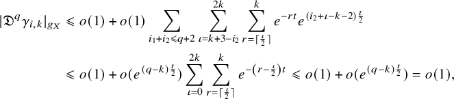 $$ \begin{align}\begin{aligned} |\mathfrak{D}^q\gamma_{i,k}|_{g_X}&\leqslant o(1)+ o(1)\sum_{i_1+i_2\leqslant q+2}\sum_{\iota=k+3-i_2}^{2k}\sum_{r=\lceil\frac{\iota}{2}\rceil}^{k}e^{-r t}e^{(i_2+\iota-k-2)\frac{t}{2}}\\ &\leqslant o(1)+o(e^{(q-k)\frac{t}{2}})\sum_{\iota=0}^{2k}\sum_{r=\lceil\frac{\iota}{2}\rceil}^{k}e^{-\left(r-\frac{\iota}{2}\right) t}\leqslant o(1)+o(e^{(q-k)\frac{t}{2}})=o(1), \end{aligned}\end{align} $$
since
 $i_2\leqslant q+2$
and
$i_2\leqslant q+2$
and
 $q\leqslant k$
. This completes the proof of Conjecture 1.1.
$q\leqslant k$
. This completes the proof of Conjecture 1.1.
5.2 Ricci curvature bounds
Next, we prove Conjecture 1.2 – namely, the Ricci curvature bound for
 $\omega ^{\bullet }(t)$
on compact subsets of
$\omega ^{\bullet }(t)$
on compact subsets of
 $X\backslash f(S)$
, which in our setting translates to
$X\backslash f(S)$
, which in our setting translates to
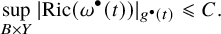 $$ \begin{align} \sup_{B\times Y}|\textrm{Ric}(\omega^{\bullet}(t))|_{g^{\bullet}(t)}\leqslant C. \end{align} $$
The argument is similar to [Reference Hein and Tosatti21, Proof of Theorem B], but there are some crucial differences coming from the time evolution in the Monge-Ampère equation, and from the fact that the bounds in (4.16) are worse than those in [Reference Hein and Tosatti21, (4.12)].
We will use the expansion (4.8) with
 $j=1$
and
$j=1$
and
 $k\geqslant 4$
(arbitrary), and with
$k\geqslant 4$
(arbitrary), and with
 $\alpha $
close to
$\alpha $
close to
 $1$
, and our first task is to improve the estimates (4.16), (4.17). These give us
$1$
, and our first task is to improve the estimates (4.16), (4.17). These give us
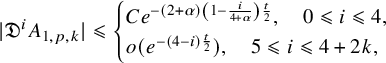 $$ \begin{align} |\mathfrak{D}^iA_{1,p,k}|\leqslant \begin{cases} Ce^{-(2+\alpha)\left(1-\frac{i}{4+\alpha}\right)\frac{t}{2}},\quad 0\leqslant i\leqslant 4,\\ o(e^{-(4-i)\frac{t}{2}}),\quad 5\leqslant i\leqslant 4+2k, \end{cases} \end{align} $$
and we can interpolate between
 $|A_{1,p,k}|\leqslant e^{-(2+\alpha )\frac {t}{2}}$
and
$|A_{1,p,k}|\leqslant e^{-(2+\alpha )\frac {t}{2}}$
and
 $[\mathfrak {D}^2A_{1,p,k}]_{C^{\alpha }}\leqslant Ce^{-t}$
from (4.18) and get
$[\mathfrak {D}^2A_{1,p,k}]_{C^{\alpha }}\leqslant Ce^{-t}$
from (4.18) and get
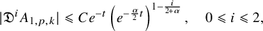 $$ \begin{align} |\mathfrak{D}^i A_{1,p,k}|\leqslant Ce^{-t}\left(e^{-\frac{\alpha}{2}t}\right)^{1-\frac{i}{2+\alpha}}, \quad 0\leqslant i\leqslant 2, \end{align} $$
so in particular, we have
 $|\dot {A}_{1,p,k}|=o(e^{-t}).$
The next claim is that
$|\dot {A}_{1,p,k}|=o(e^{-t}).$
The next claim is that
 $$ \begin{align} |\gamma_{1,k}|_{g_X}=o(e^{-t}). \end{align} $$
Indeed, using the decomposition in (5.3),
 $$ \begin{align} |\gamma_{1,k}|_{g_X}\leqslant C\sum_{i_2=0}^2\sum_{p=1}^{N_{1,k}}\sum_{\iota=0}^{2k}\sum_{r=\lceil\frac{\iota}{2}\rceil}^{2}e^{-r t}|{\mathbb{D}}^{i_2+\iota} A_{1,p,k}|, \end{align} $$
and we bound the RHS of (5.9) by
 $o(e^{-t})$
by considering the possible values of
$o(e^{-t})$
by considering the possible values of
 $i_2+\iota \in \{0,\dots ,2k+2\}$
: if
$i_2+\iota \in \{0,\dots ,2k+2\}$
: if
 $i_2+\iota =0,1,2$
, then (5.7) in particular gives
$i_2+\iota =0,1,2$
, then (5.7) in particular gives
 $|{\mathbb {D}}^{i_2+\iota } A_{1,p,k}|=o(e^{-t})$
, which is acceptable. If
$|{\mathbb {D}}^{i_2+\iota } A_{1,p,k}|=o(e^{-t})$
, which is acceptable. If
 $i_2+\iota =3,4$
, then necessarily
$i_2+\iota =3,4$
, then necessarily
 $\iota \geqslant 1$
and so
$\iota \geqslant 1$
and so
 $r\geqslant 1$
, while (5.6) in particular gives
$r\geqslant 1$
, while (5.6) in particular gives
 $|{\mathbb {D}}^{i_2+\iota } A_{1,p,k}|=o(1)$
so the RHS of (5.9) is again
$|{\mathbb {D}}^{i_2+\iota } A_{1,p,k}|=o(1)$
so the RHS of (5.9) is again
 $o(e^{-t})$
. And if
$o(e^{-t})$
. And if
 $i_2+\iota \geqslant 5$
, then we use (5.6) exactly as in (5.4) to bound the RHS of (5.9) by
$i_2+\iota \geqslant 5$
, then we use (5.6) exactly as in (5.4) to bound the RHS of (5.9) by
 $$ \begin{align} o(e^{-t})+o(1)\sum_{i_2=0}^2\sum_{p=1}^{N_{1,k}}\sum_{\iota=5-i_2}^{2k}\sum_{r=\lceil\frac{\iota}{2}\rceil}^{k}e^{-r t}e^{(i_2+\iota-4)\frac{t}{2}} \leqslant o(e^{-t})+o(e^{-t})\sum_{\iota=3}^{2k}\sum_{r=\lceil\frac{\iota}{2}\rceil}^{k}e^{-\left(r-\frac{\iota}{2}\right) t}=o(e^{-t}), \end{align} $$
since
 $i_2\leqslant 2$
, which concludes the proof of (5.8). Next, we want to show that
$i_2\leqslant 2$
, which concludes the proof of (5.8). Next, we want to show that
 $$ \begin{align} (\gamma_{1,k})_{\mathbf{ff}}=\sum_{p=1}^{N_{1,k}}A_{1,p,k}\partial_{\mathbf{f}}\overline{\partial}_{\mathbf{f}}(\Delta^{\omega_F|_{\{\cdot\}\times Y}})^{-1}G_{1,p,k}+ o(e^{-2t}), \end{align} $$
where the
 $o(e^{-2t})$
is in
$o(e^{-2t})$
is in
 $L^\infty _{\mathrm {loc}}(g_X)$
. Indeed from (5.2), we can write
$L^\infty _{\mathrm {loc}}(g_X)$
. Indeed from (5.2), we can write
 $$ \begin{align} (\gamma_{1,k})_{\mathbf{ff}}=\sum_{p=1}^{N_{1,k}}\sum_{\iota=0}^{2k}\sum_{r=\lceil\frac{\iota}{2}\rceil}^{k}e^{-r t}\partial_{\mathbf{f}}\overline{\partial}_{\mathbf{f}}\Phi_{\iota,r}(G_{1,p,k})\circledast{\mathbb{D}}^\iota A_{1,p,k}, \end{align} $$
and we can estimate each term as follows. For
 $\iota \geqslant 4$
, we have
$\iota \geqslant 4$
, we have
 $|{\mathbb {D}}^\iota A_{1,p,k}|=o(e^{-(4-\iota )\frac {t}{2}})$
from (5.6), and so
$|{\mathbb {D}}^\iota A_{1,p,k}|=o(e^{-(4-\iota )\frac {t}{2}})$
from (5.6), and so
 $$ \begin{align} e^{-r t}|\partial_{\mathbf{f}}\overline{\partial}_{\mathbf{f}}\Phi_{\iota,r}(G_{1,p,k})\circledast{\mathbb{D}}^\iota A_{1,p,k}|_{g_X}\leqslant o(1)e^{-2t}e^{-\left(r-\frac{\iota}{2}\right)t}=o(e^{-2t}), \end{align} $$
since
 $r\geqslant \frac {\iota }{2}$
. For
$r\geqslant \frac {\iota }{2}$
. For
 $\iota =3$
, we have
$\iota =3$
, we have
 $r\geqslant 2$
and
$r\geqslant 2$
and
 $|{\mathbb {D}}^\iota A_{1,p,k}|=o(1)$
from (5.6), so the term is again
$|{\mathbb {D}}^\iota A_{1,p,k}|=o(1)$
from (5.6), so the term is again
 $o(e^{-2t})$
. For
$o(e^{-2t})$
. For
 $\iota =1,2$
, we have
$\iota =1,2$
, we have
 $r\geqslant 1$
and
$r\geqslant 1$
and
 $|{\mathbb {D}}^\iota A_{1,p,k}|=o(e^{-t})$
from (5.7), so the term is again
$|{\mathbb {D}}^\iota A_{1,p,k}|=o(e^{-t})$
from (5.7), so the term is again
 $o(e^{-2t})$
. And for
$o(e^{-2t})$
. And for
 $\iota =0$
, let us first look at the terms with
$\iota =0$
, let us first look at the terms with
 $r\geqslant 1$
. For these, we have
$r\geqslant 1$
. For these, we have
 $|A_{1,p,k}|=O(e^{-(2+\alpha )\frac {t}{2}})$
, and so when multiplied by
$|A_{1,p,k}|=O(e^{-(2+\alpha )\frac {t}{2}})$
, and so when multiplied by
 $e^{-r t},r\geqslant 1$
, these terms are indeed
$e^{-r t},r\geqslant 1$
, these terms are indeed
 $o(e^{-2t})$
. So we are only left with the terms where
$o(e^{-2t})$
. So we are only left with the terms where
 $\iota =r=0$
which equal
$\iota =r=0$
which equal
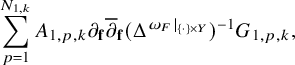 $$ \begin{align} \sum_{p=1}^{N_{1,k}}A_{1,p,k}\partial_{\mathbf{f}}\overline{\partial}_{\mathbf{f}}(\Delta^{\omega_F|_{\{\cdot\}\times Y}})^{-1}G_{1,p,k}, \end{align} $$
since
 $\Phi _{0,0}(G)=(\Delta ^{\omega _F|_{\{\cdot \}\times Y}})^{-1}G$
by (3.2), thus proving (5.11). In particular, using the bound (5.6) in (5.11) gives
$\Phi _{0,0}(G)=(\Delta ^{\omega _F|_{\{\cdot \}\times Y}})^{-1}G$
by (3.2), thus proving (5.11). In particular, using the bound (5.6) in (5.11) gives
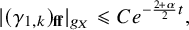 $$ \begin{align} |(\gamma_{1,k})_{\mathbf{ff}}|_{g_X}\leqslant Ce^{-\frac{2+\alpha}{2}t}, \end{align} $$
while tracing (5.11) fiberwise gives
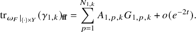 $$ \begin{align} \mathrm{tr}_{\omega_F|_{\{\cdot\}\times Y}}(\gamma_{1,k})_{\mathbf{ff}}=\sum_{p=1}^{N_{1,k}}A_{1,p,k}G_{1,p,k} + o(e^{-2t}). \end{align} $$
Before we continue with the proof of (5.5), recall that from [Reference Fong and Zhang12, p.110] (see also [Reference Tosatti39, Lemma 5.13]) we know that
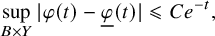 $$ \begin{align} \sup_{B\times Y}|\varphi (t)-\underline{\varphi }(t)|\leqslant Ce^{-t}, \end{align} $$
for all
 $t\geqslant 0$
. The argument in [Reference Tosatti, Weinkove and Yang43, Lemma 3.1 (iv)] then allows one to deduce from this that
$t\geqslant 0$
. The argument in [Reference Tosatti, Weinkove and Yang43, Lemma 3.1 (iv)] then allows one to deduce from this that
 $$ \begin{align} \sup_{B\times Y} |\dot{\varphi }(t)-\underline{\dot{\varphi }}(t)|\leqslant Ce^{-\frac{t}{2}}. \end{align} $$
As a consequence of our asymptotic expansion, we can now improve both of these:
Proposition 5.1. On
 $B\times Y$
, we have
$B\times Y$
, we have
 $$ \begin{align} |\varphi (t)-\underline{\varphi }(t)|=o(e^{-t}), \quad |\dot{\varphi }(t)-\underline{\dot{\varphi }}(t)|=o(e^{-t}). \end{align} $$
Proof. Recall that by definition, we can write
 $$ \begin{align} \varphi -\underline{\varphi }=\psi_{1,k}+\sum_{p=1}^{N_{1,k}}\mathfrak{G}_{t,k}(A_{1,p,k},G_{1,p,k}), \end{align} $$
and we want to bound the
 $L^\infty $
norm of the two terms on the RHS of (5.20) and their time derivatives. For
$L^\infty $
norm of the two terms on the RHS of (5.20) and their time derivatives. For
 $\psi _{1,k}$
, from (4.9), we have
$\psi _{1,k}$
, from (4.9), we have
 $$ \begin{align} |{i\partial\bar\partial}\psi_{1,k}|_{g(t)}\leqslant e^{-(1+\frac{\alpha}{2})t}, \end{align} $$
so restricting this to a fiber
 $\{z\}\times Y$
gives
$\{z\}\times Y$
gives
 $$ \begin{align} |{i\partial\bar\partial}\psi_{1,k}|_{\{z\}\times Y}|_{g_Y}\leqslant e^{-(2+\frac{\alpha}{2})t}, \end{align} $$
and since
 $\psi _{1,k}$
has fiberwise average zero, applying Moser iteration on
$\psi _{1,k}$
has fiberwise average zero, applying Moser iteration on
 $\{z\}\times Y$
(with constant that does not depend on
$\{z\}\times Y$
(with constant that does not depend on
 $z\in B$
) gives
$z\in B$
) gives
 $$ \begin{align} |\psi_{1,k}|\leqslant Ce^{-(2+\frac{\alpha}{2})t}. \end{align} $$
Arguing similarly for
 $\dot {\psi }$
, which by (4.9) satisfies (since
$\dot {\psi }$
, which by (4.9) satisfies (since
 $k\geqslant 4$
)
$k\geqslant 4$
)
 $$ \begin{align} |{i\partial\bar\partial}\dot{\psi}_{1,k}|_{g(t)}\leqslant e^{-\frac{\alpha}{2}t}, \end{align} $$
we get
 $$ \begin{align} |\dot{\psi}_{1,k}|\leqslant Ce^{-(1+\frac{\alpha}{2})t}. \end{align} $$
As for the term
 $\mathfrak {G}_{t,k}(A_{1,p,k},G_{1,p,k})$
, using again (5.2), we can write it as
$\mathfrak {G}_{t,k}(A_{1,p,k},G_{1,p,k})$
, using again (5.2), we can write it as
 $$ \begin{align} \sum_{\iota=0}^{2k}\sum_{r=\lceil\frac{\iota}{2}\rceil}^{k}e^{-r t}\Phi_{\iota,r}(G_{1,p,k})\circledast{\mathbb{D}}^\iota A_{1,p,k}, \end{align} $$
and using (5.6) and (5.7), we can argue similarly to the proof of (5.8) and bound
 $$ \begin{align} |\mathfrak{G}_{t,k}(A_{1,p,k},G_{1,p,k})|\leqslant C \sum_{\iota=0}^{2k}\sum_{r=\lceil\frac{\iota}{2}\rceil}^{k}e^{-r t}|{\mathbb{D}}^\iota A_{1,p,k}|, \end{align} $$
by
 $o(e^{-t})$
by considering the possible values of
$o(e^{-t})$
by considering the possible values of
 $\iota \in \{0,\dots ,2k\}$
: if
$\iota \in \{0,\dots ,2k\}$
: if
 $\iota =0$
, then (5.6) in particular gives
$\iota =0$
, then (5.6) in particular gives
 $|A_{1,p,k}|=o(e^{-t})$
, which is acceptable. If
$|A_{1,p,k}|=o(e^{-t})$
, which is acceptable. If
 $1\leqslant \iota \leqslant 4$
, then necessarily
$1\leqslant \iota \leqslant 4$
, then necessarily
 $r\geqslant 1$
, while (5.6) in particular gives
$r\geqslant 1$
, while (5.6) in particular gives
 $|{\mathbb {D}}^{\iota } A_{1,p,k}|=o(1)$
so the RHS of (5.27) is again
$|{\mathbb {D}}^{\iota } A_{1,p,k}|=o(1)$
so the RHS of (5.27) is again
 $o(e^{-t})$
. And if
$o(e^{-t})$
. And if
 $\iota \geqslant 5$
, then we use (5.6) to bound the RHS of (5.27) by
$\iota \geqslant 5$
, then we use (5.6) to bound the RHS of (5.27) by
 $$ \begin{align} o(e^{-t})+o(1)\sum_{p=1}^{N_{1,k}}\sum_{\iota=5}^{2k}\sum_{r=\lceil\frac{\iota}{2}\rceil}^{k}e^{-r t}e^{(\iota-4)\frac{t}{2}} \leqslant o(e^{-t})+o(e^{-2t})\sum_{\iota=5}^{2k}\sum_{r=\lceil\frac{\iota}{2}\rceil}^{k}e^{-\left(r-\frac{\iota}{2}\right) t}=o(e^{-t})+o(e^{-2t}), \end{align} $$
and so
 $$ \begin{align} \mathfrak{G}_{t,k}(A_{1,p,k},G_{1,p,k})=o(e^{-t}). \end{align} $$
Similarly,
 $$ \begin{align} \mathfrak{G}_{t,k}(\dot{A}_{1,p,k},G_{1,p,k})=\sum_{\iota=0}^{2k}\sum_{r=\lceil\frac{\iota}{2}\rceil}^{k}e^{-r t}\Phi_{\iota,r}(G_{1,p,k})\circledast{\mathbb{D}}^\iota \dot{A}_{1,p,k}, \end{align} $$
and we argue as above to show that this is
 $o(e^{-t})$
: if
$o(e^{-t})$
: if
 $\iota =0$
, then (5.7) in particular gives
$\iota =0$
, then (5.7) in particular gives
 $|\dot {A}_{1,p,k}|=o(e^{-t})$
, which is acceptable. If
$|\dot {A}_{1,p,k}|=o(e^{-t})$
, which is acceptable. If
 $1\leqslant \iota \leqslant 2$
, then
$1\leqslant \iota \leqslant 2$
, then
 $r\geqslant 1$
, while (5.6) in particular gives
$r\geqslant 1$
, while (5.6) in particular gives
 $|{\mathbb {D}}^{\iota } \dot {A}_{1,p,k}|=o(1)$
so the RHS of (5.30) is again
$|{\mathbb {D}}^{\iota } \dot {A}_{1,p,k}|=o(1)$
so the RHS of (5.30) is again
 $o(e^{-t})$
. And if
$o(e^{-t})$
. And if
 $\iota \geqslant 3$
, then we use (5.6) to bound the RHS of (5.30) by
$\iota \geqslant 3$
, then we use (5.6) to bound the RHS of (5.30) by
 $$ \begin{align} o(e^{-t})+o(1)\sum_{p=1}^{N_{1,k}}\sum_{\iota=3}^{2k}\sum_{r=\lceil\frac{\iota}{2}\rceil}^{k}e^{-r t}e^{(\iota-2)\frac{t}{2}} \leqslant o(e^{-t})\sum_{\iota=3}^{2k}\sum_{r=\lceil\frac{\iota}{2}\rceil}^{k}e^{-\left(r-\frac{\iota}{2}\right) t}=o(e^{-t}), \end{align} $$
and so
 $$ \begin{align} \mathfrak{G}_{t,k}(\dot{A}_{1,p,k},G_{1,p,k})=o(e^{-t}). \end{align} $$
Combining (5.20) with (5.23), (5.25), (5.29) and (5.32) we see that (5.19) holds.
Remark 5.2. If we use the stronger bounds (5.55), (5.56) for derivatives of
 $A_{1,p,k}$
, which will be established below, we can then repeat the proof of Proposition 5.1, and we get the better bounds
$A_{1,p,k}$
, which will be established below, we can then repeat the proof of Proposition 5.1, and we get the better bounds
 $$ \begin{align} |\varphi (t)-\underline{\varphi }(t)|\leqslant Ce^{-2t}, \quad |\dot{\varphi }(t)-\underline{\dot{\varphi }}(t)|\leqslant Ce^{-(1+\frac{\gamma}{2})t}, \end{align} $$
where
 $\gamma =\frac {\alpha }{4+\alpha }>0.$
Now that (5.19) is established, we can use it to prove the next claim, which is the analog of [Reference Hein and Tosatti21, (5.26)]:
Proposition 5.3. We have
 $$ \begin{align} |A_{1,p,k}|\leqslant Ce^{-2t}. \end{align} $$
Proof. First, observe that thanks to (4.9), we have
 $$ \begin{align} |\eta_{1,k}|_{g(t)}\leqslant e^{-(2+\alpha)\frac{t}{2}}, \end{align} $$
which implies that
 $$ \begin{align} |\eta_{1,k}|_{g_X}=o(e^{-t}),\quad |(\eta_{1,k})_{\mathbf{ff}}|_{g_X}=o(e^{-2t}), \end{align} $$
and combining this with (5.8) and (5.15), we get
 $$ \begin{align} |e^t\gamma_{1,k}+e^t\eta_{1,k}|_{g_X}=o(1),\quad |(e^t\gamma_{1,k}+e^t\eta_{1,k})_{\mathbf{ff}}|_{g_X}=O(e^{-\alpha\frac{t}{2}}). \end{align} $$
The Monge-Ampère equation (4.1) that describes the flow can be written as
 $$ \begin{align} e^{\varphi (t)+\dot{\varphi }(t)}e^{-nt}\binom{m+n}{n}\omega_{\mathrm{can}}^m\wedge\omega_F^n=(\omega_{\mathrm{can}}+e^{-t}\omega_F+{i\partial\bar\partial} \underline{\varphi }(t)+\gamma_{1,k}(t)+\eta_{1,k}(t))^{m+n}, \end{align} $$
and multiplying this by
 $\frac {e^{nt}}{\binom {m+n}{n}}$
, expanding it out, and using that
$\frac {e^{nt}}{\binom {m+n}{n}}$
, expanding it out, and using that
 ${i\partial \bar \partial } \underline{\varphi }(t)$
is small in
${i\partial \bar \partial } \underline{\varphi }(t)$
is small in
 $C^2$
by (4.12), as well as (5.36), (5.37), we see that
$C^2$
by (4.12), as well as (5.36), (5.37), we see that
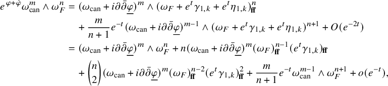 $$ \begin{align}\begin{aligned} e^{\varphi +\dot{\varphi }}\omega_{\mathrm{can}}^m\wedge\omega_F^n&=(\omega_{\mathrm{can}}+{i\partial\bar\partial}\underline{\varphi })^m\wedge(\omega_F+e^t\gamma_{1,k}+e^t\eta_{1,k})_{\mathbf{ff}}^n\\&\quad+\frac{m}{n+1}e^{-t} (\omega_{\mathrm{can}}+{i\partial\bar\partial}\underline{\varphi })^{m-1}\wedge(\omega_F+e^t\gamma_{1,k}+e^t\eta_{1,k})^{n+1}+O(e^{-2t})\\&=(\omega_{\mathrm{can}}+{i\partial\bar\partial}\underline{\varphi })^m\wedge\omega_F^n+ n(\omega_{\mathrm{can}}+{i\partial\bar\partial}\underline{\varphi })^m(\omega_F)_{\mathbf{ff}}^{n-1}(e^t\gamma_{1,k})_{\mathbf{ff}}\\&\quad+\binom{n}{2}(\omega_{\mathrm{can}}+{i\partial\bar\partial}\underline{\varphi })^m(\omega_F)_{\mathbf{ff}}^{n-2}(e^t\gamma_{1,k})_{\mathbf{ff}}^2+\frac{m}{n+1}e^{-t} \omega_{\mathrm{can}}^{m-1}\wedge\omega_F^{n+1}+o(e^{-t}), \end{aligned}\end{align} $$
where the error terms
 $o(e^{-t})$
are in
$o(e^{-t})$
are in
 $L^\infty _{\mathrm {loc}}(g_X)$
. We used here that
$L^\infty _{\mathrm {loc}}(g_X)$
. We used here that
 $\alpha>\frac {2}{3}$
, so that
$\alpha>\frac {2}{3}$
, so that
 $|(e^t\gamma _{1,k})_{\mathbf {ff}}^p|=o(e^{-t})$
for
$|(e^t\gamma _{1,k})_{\mathbf {ff}}^p|=o(e^{-t})$
for
 $p\geqslant 3$
by (5.15). As in [Reference Hein and Tosatti21, (5.29)], we define a function
$p\geqslant 3$
by (5.15). As in [Reference Hein and Tosatti21, (5.29)], we define a function
 $\mathcal {S}$
by
$\mathcal {S}$
by
 $$ \begin{align} \frac{m}{n+1}\omega_{\mathrm{can}}^{m-1}\wedge\omega_F^{n+1}=\mathcal{S}\omega_{\mathrm{can}}^{m}\wedge\omega_F^{n}, \end{align} $$
so that dividing (5.39) by the volume form
 $\omega _{\mathrm {can}}^m\wedge \omega _F^n$
and multiplying by
$\omega _{\mathrm {can}}^m\wedge \omega _F^n$
and multiplying by
 $e^{-t}$
gives
$e^{-t}$
gives
 $$ \begin{align} e^{-t}e^{\varphi +\dot{\varphi }}=\left(e^{-t}+\operatorname{tr}_{\omega_F|_{\{\cdot\}\times Y}}(\gamma_{1,k})_{\mathbf{ff}}+e^{-t}\frac{\binom{n}{2}(\omega_F)_{\mathbf{ff}}^{n-2}(e^t\gamma_{1,k})_{\mathbf{ff}}^2}{(\omega_F)_{\mathbf{ff}}^{n}}+e^{-2t}\mathcal{S}\right)(1+o(1)_{\mathrm{base}})+o(e^{-2t}), \end{align} $$
and subtracting from (5.41) its fiber average (the two terms with
 $\gamma _{1,k}$
have fiberwise average zero since
$\gamma _{1,k}$
have fiberwise average zero since
 $\gamma _{1,k}$
is
$\gamma _{1,k}$
is
 $\partial \overline {\partial }$
-exact) and using (5.16) gives
$\partial \overline {\partial }$
-exact) and using (5.16) gives
 $$ \begin{align} e^{-t}(e^{\varphi +\dot{\varphi }}-\underline{e^{\varphi +\dot{\varphi }}})=\left(\sum_{p=1}^{N_{1,k}}A_{1,p,k}G_{1,p,k} +e^{-t}\frac{\binom{n}{2}(\omega_F)_{\mathbf{ff}}^{n-2}(e^t\gamma_{1,k})_{\mathbf{ff}}^2}{(\omega_F)_{\mathbf{ff}}^{n}}+e^{-2t}(\mathcal{S}-\underline{\mathcal{S}})\right)(1+o(1)_{\mathrm{base}})+o(e^{-2t}). \end{align} $$
To bound the LHS of (5.42), use the Taylor expansion of the exponential, together with Lemma 4.1 (ii) and (5.19) to bound
 $$ \begin{align} e^{-t}|e^{\varphi +\dot{\varphi }}-\underline{e^{\varphi +\dot{\varphi }}}|\leqslant Ce^{-t}|\varphi +\dot{\varphi }-\underline{\varphi +\dot{\varphi }}|=o(e^{-2t}), \end{align} $$
while on the RHS of (5.42), we can bound
 $$ \begin{align} e^{-t}\left|\frac{\binom{n}{2}(\omega_F)_{\mathbf{ff}}^{n-2}(e^t\gamma_{1,k})_{\mathbf{ff}}^2}{(\omega_F)_{\mathbf{ff}}^{n}}\right|\leqslant Ce^{-t}|(e^t\gamma_{1,k})_{\mathbf{ff}}^2|\leqslant Ce^{-(1+\alpha)t}, \end{align} $$
by (5.15). Thus, going back to (5.42), we learn that
 $$ \begin{align} \sum_{p=1}^{N_{1,k}}A_{1,p,k}G_{1,p,k}=O(e^{-(1+\alpha)t}), \end{align} $$
and taking the fiberwise
 $L^2$
inner product with each
$L^2$
inner product with each
 $G_{1,p,k}$
, we see that
$G_{1,p,k}$
, we see that
 $$ \begin{align} A_{1,p,k}=O(e^{-(1+\alpha)t}), \end{align} $$
which improves over the bound
 $A_{1,p,k}=O(e^{-(1+\frac {\alpha }{2})t})$
from (5.6). We can then go back to (5.11) and see that
$A_{1,p,k}=O(e^{-(1+\frac {\alpha }{2})t})$
from (5.6). We can then go back to (5.11) and see that
 $$ \begin{align} |(\gamma_{1,k})_{\mathbf{ff}}|_{g_X}\leqslant Ce^{-(1+\alpha)t}, \end{align} $$
which allows us to improve (5.37) to
 $$ \begin{align} |(e^t\gamma_{1,k}+e^t\eta_{1,k})_{\mathbf{ff}}|_{g_X}=O(e^{-\alpha t}), \end{align} $$
and so as long as we choose
 $\alpha>\frac {1}{2}$
, we see that
$\alpha>\frac {1}{2}$
, we see that
 $$ \begin{align} |(e^t\gamma_{1,k})_{\mathbf{ff}}^2|_{g_X}=o(e^{-t}), \end{align} $$
and so in (5.42), we have
 $$ \begin{align} e^{-t}\left|\frac{\binom{n}{2}(\omega_F)_{\mathbf{ff}}^{n-2}(e^t\gamma_{1,k})_{\mathbf{ff}}^2}{(\omega_F)_{\mathbf{ff}}^{n}}\right|\leqslant Ce^{-t}|(e^t\gamma_{1,k})_{\mathbf{ff}}^2|=o(e^{-2t}), \end{align} $$
and returning to (5.42) again, we see that
 $$ \begin{align} \sum_{p=1}^{N_{1,k}}A_{1,p,k}G_{1,p,k}=O(e^{-2t}), \end{align} $$
and again taking the fiberwise inner product with each
 $G_{1,p,k}$
concludes the proof of (5.34).
$G_{1,p,k}$
concludes the proof of (5.34).
Next, observe that from (4.9) we have in particular
 $$ \begin{align} |\mathfrak{D}^i\eta_{1,k}|_{g(t)}\leqslant Ce^{\frac{i-2-\alpha}{2}t},\quad 0\leqslant i\leqslant 2. \end{align} $$
We want to show a similar estimate for
 $\gamma _{1,k}$
which is only slightly worse:
$\gamma _{1,k}$
which is only slightly worse:
Proposition 5.4. We have
 $$ \begin{align} |\mathfrak{D}^i\gamma_{1,k}|_{g(t)}\leqslant Ce^{\frac{i-2}{2}t},\quad 0\leqslant i\leqslant 2, \end{align} $$
and also
 $$ \begin{align} |\dot{\gamma}_{1,k}|_{g(t)}\leqslant C e^{-\gamma\frac{t}{2}}, \end{align} $$
where
 $\gamma =\frac {\alpha }{4+\alpha }>0$
.
$\gamma =\frac {\alpha }{4+\alpha }>0$
.
Proof. The first step is to use (5.34) to improve the estimates in (5.6), by interpolating it with
 $[\mathfrak {D}^4 A_{1,p,k}]_{C^{\alpha }}\leqslant C$
from (4.18) and get
$[\mathfrak {D}^4 A_{1,p,k}]_{C^{\alpha }}\leqslant C$
from (4.18) and get
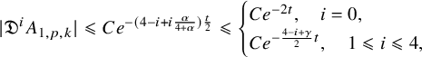 $$ \begin{align} |\mathfrak{D}^iA_{1,p,k}|\leqslant Ce^{-(4-i+i\frac{\alpha}{4+\alpha})\frac{t}{2}}\leqslant\begin{cases} Ce^{-2t},\quad i=0,\\ Ce^{-\frac{4-i+\gamma}{2}t}, \quad 1\leqslant i\leqslant 4, \end{cases} \end{align} $$
where
 $\gamma =\frac {\alpha }{4+\alpha }>0$
. As for higher order derivatives of
$\gamma =\frac {\alpha }{4+\alpha }>0$
. As for higher order derivatives of
 $A_{1,p,k}$
, given
$A_{1,p,k}$
, given
 $1\leqslant \iota \leqslant 2k$
, we interpolate between
$1\leqslant \iota \leqslant 2k$
, we interpolate between
 $|\mathfrak {D}^4A_{1,p,k}|\leqslant Ce^{-\frac {\gamma }{2}t}$
from (5.55) and
$|\mathfrak {D}^4A_{1,p,k}|\leqslant Ce^{-\frac {\gamma }{2}t}$
from (5.55) and
 $[\mathfrak {D}^{4+\iota }A_{1,p,k}]_{C^{\alpha }}\leqslant Ce^{\frac {\iota }{2}t}$
from (4.18) and letting
$[\mathfrak {D}^{4+\iota }A_{1,p,k}]_{C^{\alpha }}\leqslant Ce^{\frac {\iota }{2}t}$
from (4.18) and letting
 $i=4+\iota $
, we get
$i=4+\iota $
, we get
 $$ \begin{align} |\mathfrak{D}^i A_{1,p,k}|\leqslant Ce^{-\frac{4-i+\gamma}{2}t}, \quad 5\leqslant i\leqslant 4+2k. \end{align} $$
Finally, using (5.55) and (5.56), we can bound
 $|\mathfrak {D}^i\gamma _{1,k}|_{g(t)}, 0\leqslant i\leqslant 2,$
by going back to (5.3) and bounding
$|\mathfrak {D}^i\gamma _{1,k}|_{g(t)}, 0\leqslant i\leqslant 2,$
by going back to (5.3) and bounding
 $$ \begin{align} |\mathfrak{D}^i\gamma_{1,k}|_{g(t)}\leqslant \sum_{p=1}^{N_{1,k}}\sum_{\iota=0}^{2k}\sum_{r=\lceil\frac{\iota}{2}\rceil}^{k}\sum_{s=0}^{i+1}\sum_{i_1+i_2=s+1}e^{-r t}|({\mathbb{D}}^{i+1-s}J)|_{g(t)} |{\mathbb{D}}^{i_1}\Phi_{\iota,r}(G_{1,p,k})|_{g(t)} |\mathfrak{D}^{i_2+\iota} A_{1,p,k}|_{g(t)}, \end{align} $$
and using also
 $|{\mathbb {D}}^{i_1}\Phi _{\iota ,r}(G_{1,p,k})|_{g(t)}\leqslant Ce^{i_1\frac {t}{2}}$
,
$|{\mathbb {D}}^{i_1}\Phi _{\iota ,r}(G_{1,p,k})|_{g(t)}\leqslant Ce^{i_1\frac {t}{2}}$
,
 $|{\mathbb {D}}^\iota J|_{g(t)}\leqslant Ce^{\iota \frac {t}{2}},$
we get
$|{\mathbb {D}}^\iota J|_{g(t)}\leqslant Ce^{\iota \frac {t}{2}},$
we get
 $$ \begin{align} |\mathfrak{D}^i\gamma_{1,k}|_{g(t)}\leqslant C\sum_{\iota=0}^{2k}\sum_{r=\lceil\frac{\iota}{2}\rceil}^{k}\sum_{s=0}^{i+1}\sum_{i_1+i_2=s+1}e^{-r t}e^{(i_1+i_2+i+1-s+\iota-4)\frac{t}{2}} \leqslant Ce^{(i-2)\frac{t}{2}}\sum_{\iota=0}^{2k}\sum_{r=\lceil\frac{\iota}{2}\rceil}^{k}e^{-\left(r-\frac{\iota}{2}\right)t}\leqslant Ce^{(i-2)\frac{t}{2}}, \end{align} $$
for
 $0\leqslant i\leqslant 2$
, which proves (5.53). As for (5.54), using (5.3) again, we can bound
$0\leqslant i\leqslant 2$
, which proves (5.53). As for (5.54), using (5.3) again, we can bound
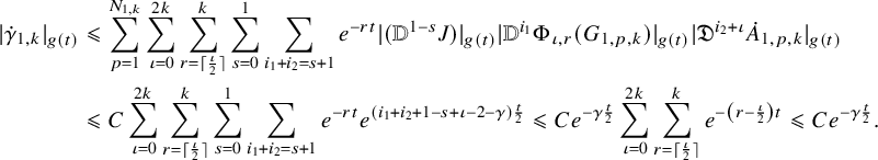 $$ \begin{align}\begin{aligned} |\dot{\gamma}_{1,k}|_{g(t)}&\leqslant \sum_{p=1}^{N_{1,k}}\sum_{\iota=0}^{2k}\sum_{r=\lceil\frac{\iota}{2}\rceil}^{k}\sum_{s=0}^{1}\sum_{i_1+i_2=s+1}e^{-r t}|({\mathbb{D}}^{1-s}J)|_{g(t)} |{\mathbb{D}}^{i_1}\Phi_{\iota,r}(G_{1,p,k})|_{g(t)} |\mathfrak{D}^{i_2+\iota} \dot{A}_{1,p,k}|_{g(t)}\\ &\leqslant C\sum_{\iota=0}^{2k}\sum_{r=\lceil\frac{\iota}{2}\rceil}^{k}\sum_{s=0}^{1}\sum_{i_1+i_2=s+1}e^{-r t}e^{(i_1+i_2+1-s+\iota-2-\gamma)\frac{t}{2}} \leqslant Ce^{-\gamma\frac{t}{2}}\sum_{\iota=0}^{2k}\sum_{r=\lceil\frac{\iota}{2}\rceil}^{k}e^{-\left(r-\frac{\iota}{2}\right)t}\leqslant Ce^{-\gamma\frac{t}{2}}. \end{aligned} \end{align} $$
After these preparations, we can finally give the proof of the Ricci curvature bound (5.5). For this, we take
 ${i\partial \bar \partial }\log $
of the Monge-Ampère equation (4.1) and get
${i\partial \bar \partial }\log $
of the Monge-Ampère equation (4.1) and get
 $$ \begin{align}\begin{aligned} \textrm{Ric}(\omega^{\bullet}(t))&=-{i\partial\bar\partial}\log\det g^{\bullet}(t)\\ &=-{i\partial\bar\partial}\log(\omega_{\mathrm{can}}^m\wedge\omega_F^n)-{i\partial\bar\partial}(\varphi (t)+\dot{\varphi }(t))\\ &=-\omega_{\mathrm{can}}-{i\partial\bar\partial}(\varphi (t)+\dot{\varphi }(t))\\ &=-\omega^{\bullet}(t)+e^{-t}\omega_F-{i\partial\bar\partial}\dot{\varphi }(t), \end{aligned} \end{align} $$
where we used the known relation
 $-{i\partial \bar \partial }\log (\omega _{\mathrm { can}}^m\wedge \omega _F^n)=-\omega _{\mathrm {can}}$
(see, for example, [Reference Tosatti39, Proposition 5.9]). Since
$-{i\partial \bar \partial }\log (\omega _{\mathrm { can}}^m\wedge \omega _F^n)=-\omega _{\mathrm {can}}$
(see, for example, [Reference Tosatti39, Proposition 5.9]). Since
 $\omega ^{\bullet }(t)$
is uniformly equivalent to
$\omega ^{\bullet }(t)$
is uniformly equivalent to
 $\omega ^\natural (t)$
(by Lemma 4.1 (i)), it suffices to bound
$\omega ^\natural (t)$
(by Lemma 4.1 (i)), it suffices to bound
 $|\textrm {Ric}(\omega ^{\bullet }(t))|_{g^\natural (t)}$
on compact subsets of
$|\textrm {Ric}(\omega ^{\bullet }(t))|_{g^\natural (t)}$
on compact subsets of
 $X\backslash S$
. We can then work on
$X\backslash S$
. We can then work on
 $B\times Y$
as before, where we may assume that we have the expansion (4.8) with
$B\times Y$
as before, where we may assume that we have the expansion (4.8) with
 $j=1$
and
$j=1$
and
 $k\geqslant 4$
,
$k\geqslant 4$
,
 $$ \begin{align}\omega^{\bullet}(t)=\omega^\natural(t)+\gamma_{0}(t)+\gamma_{1,k}(t)+\eta_{1,k}(t).\end{align} $$
Using (4.12), (5.52) and (5.53), we thus see that
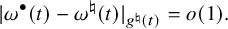 $$ \begin{align} |\omega^{\bullet}(t)-\omega^\natural(t)|_{g^\natural(t)}=o(1). \end{align} $$
Taking a time derivative of (5.61), we obtain
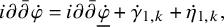 $$ \begin{align} {i\partial\bar\partial}\dot{\varphi }={i\partial\bar\partial}\underline{\dot{\varphi }}+\dot{\gamma}_{1,k}+\dot{\eta}_{1,k}, \end{align} $$
and using (4.12), (5.52), (5.54), we see that
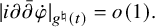 $$ \begin{align} |{i\partial\bar\partial}\dot{\varphi }|_{g^\natural(t)}=o(1). \end{align} $$
Thus, going back to (5.60), we can write
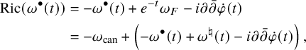 $$ \begin{align}\begin{aligned} \textrm{Ric}(\omega^{\bullet}(t))&=-\omega^{\bullet}(t)+e^{-t}\omega_F-{i\partial\bar\partial}\dot{\varphi }(t)\\ &=-\omega_{\mathrm{can}}+\left(-\omega^{\bullet}(t)+\omega^\natural(t)-{i\partial\bar\partial}\dot{\varphi }(t)\right), \end{aligned} \end{align} $$
where thanks to (5.62) and (5.64), we have
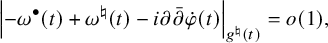 $$ \begin{align} \left|-\omega^{\bullet}(t)+\omega^\natural(t)-{i\partial\bar\partial}\dot{\varphi }(t)\right|_{g^\natural(t)}=o(1), \end{align} $$
and since we clearly have
 $|\omega _{\mathrm {can}}|_{g^\natural (t)}\leqslant C,$
the Ricci bound
$|\omega _{\mathrm {can}}|_{g^\natural (t)}\leqslant C,$
the Ricci bound
 $|\textrm {Ric}(\omega ^{\bullet }(t))|_{g^\natural (t)}\leqslant C$
follows.
$|\textrm {Ric}(\omega ^{\bullet }(t))|_{g^\natural (t)}\leqslant C$
follows.
Observe that (5.65) and (5.66) give us very detailed information about the Ricci curvature of
 $\omega ^{\bullet }(t)$
(on compact subsets of
$\omega ^{\bullet }(t)$
(on compact subsets of
 $X\backslash S$
), showing that it is asymptotic to
$X\backslash S$
), showing that it is asymptotic to
 $-\omega _{\mathrm {can}}$
in a strong sense.
$-\omega _{\mathrm {can}}$
in a strong sense.
Remark 5.5. Since
 $\omega _{\mathrm {can}}$
is pulled back from the base, and since
$\omega _{\mathrm {can}}$
is pulled back from the base, and since
 $\omega ^{\bullet }(t)\to \omega _{\mathrm {can}}$
locally uniformly (from Lemma 4.1 (i), (iii)), it follows that
$\omega ^{\bullet }(t)\to \omega _{\mathrm {can}}$
locally uniformly (from Lemma 4.1 (i), (iii)), it follows that
 $$ \begin{align} \operatorname{tr}_{\omega^{\bullet}(t)}\omega_{\mathrm{can}}\to \operatorname{tr}_{\omega_{\mathrm{can}}}\omega_{\mathrm{can}}=m, \end{align} $$
locally uniformly on
 $X\backslash S$
. Thus, taking the trace of (5.65) with respect to
$X\backslash S$
. Thus, taking the trace of (5.65) with respect to
 $\omega ^{\bullet }(t)$
, we see that
$\omega ^{\bullet }(t)$
, we see that
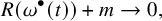 $$ \begin{align} R(\omega^{\bullet}(t))+m\to 0, \end{align} $$
in
 $C^0_{\mathrm {loc}}(X\backslash S)$
, which recovers the main theorem of [Reference Jian22].
$C^0_{\mathrm {loc}}(X\backslash S)$
, which recovers the main theorem of [Reference Jian22].
Remark 5.6. Continuing the above arguments along the lines of [Reference Hein and Tosatti21, (5.37)–(5.86)], one can also identify the first nontrivial term in the expansion (4.8) of
 $\omega ^{\bullet }(t)$
, whose shape is identical to the one in the elliptic setting; see [Reference Hein and Tosatti21, Theorem B]. For the sake of brevity, we leave the straightforward proof to the interested reader.
$\omega ^{\bullet }(t)$
, whose shape is identical to the one in the elliptic setting; see [Reference Hein and Tosatti21, Theorem B]. For the sake of brevity, we leave the straightforward proof to the interested reader.
Acknowledgements
Part of this work was carried out during visits of the second-named author to the Courant Institute of Mathematical Sciences, and of the third-named author to the Center of Mathematical Sciences and Applications at Harvard University, which we would like to thank for the hospitality. We thank J. Cheng, C. Hacon, J. Lott, S. Karigiannis and M. Păun for discussions about Remarks 1.4 and 1.5, and the referee for helpful comments on a previous version.
Competing interest
The authors have no competing interests to declare.
Funding statement
The first-named author was partially supported by the German Research Foundation (DFG) under Germany’s Excellence Strategy EXC 2044-390685587 ‘Mathematics Münster: Dynamics-Geometry-Structure’ and by the CRC 1442 ‘Geometry: Deformations and Rigidity’ of the DFG. The second-named author was partially supported by Hong Kong RGC grant (Early Career Scheme) of Hong Kong No. 24304222, No. 14300623, and an NSFC grant No. 12222122. The third-named author was partially supported by NSF grants DMS-2231783 and DMS-2404599.


 Open access