


Impact Statement
The control of the phase behaviour of ternary fluid systems represents a considerable technological challenge with the formation of complex flow and transport phenomena at the fluid interface. Systems composed of two immiscible fluids, such as water and oil, and a miscible solvent, however, are commonly employed during the formation of microemulsions and find use in a variety of industries, including in the pharmaceutical and energy sectors and in consumer products, such as food and cosmetics. While numerous studies have addressed the thermodynamic stability of ternary systems at long time scales, less is known about their out-of-equilibrium behaviour at short time scales, which limits the development of advanced functional materials. In this work, we reveal powerful flow-based microfluidic techniques for the formation of aqueous droplets and jets in solvent–oil mixtures and lay the phenomenological and mathematical foundations for the manipulation of ternary fluid systems and time-evolving soft materials in microflow reactors.
1. Introduction
Liquid multiphase flow processing techniques are commonly encountered in a wide range of industries, including in the energy and pharmaceutical domains as well as food, cosmetics, 3-D printing and material synthesis (Aubry et al. Reference Aubry, Ganachaud, Cohen Addad and Cabane2009; Zinchenko & Davis, Reference Zinchenko and Davis2017; Rauzan et al. Reference Rauzan, Nelson, Lehman, Ewoldt and Nuzzo2018). As a condensed phase of matter, the liquid state is made of closely packed molecules and the property of fluidity confers unique abilities for the transport and manipulation of basic materials, including water, oils and organic solvents. Emulsions and interfacial fluid arrangements can be controlled using a variety of tensioactive agents (Leal-Calderon et al. Reference Leal-Calderon, Schmitt and Bibette2007; Perazzo et al. Reference Perazzo, Preziosi and Guido2015). For instance, amphiphilic surfactant molecules are often added to water and oil dispersions during the formation of emulsions to reduce interfacial tension and stabilise droplets against coalescence (McClements, Reference McClements2012; Gupta et al. Reference Gupta, Eral, Hatton and Doyle2016; Kim & Mason, Reference Kim and Mason2017). Recently, solutes of different types have been shown to facilitate the fabrication of all-aqueous biocompatible materials (Song et al. Reference Song, Sauret and Shum2013). In general, however, the strong intermolecular forces present in these systems due to particulate additives introduce great complexity in the prediction of fluid interactions and flow patterns.
In the case of pure substances, the interfacial behaviour of immiscible fluids depends on the interplay of interfacial and viscous stresses (De Gennes et al. Reference De Gennes, Brochard-Wyart and Quéré2004), and capillary instabilities typically lead to the formation of dispersed flows of droplets (Eggers & Villermaux, Reference Eggers and Villermaux2008; Montanero & Gañán-Calvo, Reference Montanero and Gañán-Calvo2020). By contrast, when fluids are miscible, the interface is diffuse and separated flows, such as core–annular and layered flows, readily form depending on fluid viscosities and flow velocity (Selvam et al. Reference Selvam, Merk, Govindarajan and Meiburg2007; Hu & Cubaud, Reference Hu and Cubaud2018; Salin & Talon, Reference Salin and Talon2019). Diverse advection–diffusion phenomena are also observed between miscible fluids during displacement and transport in porous-like media (Lajeunesse et al. Reference Lajeunesse, Martin, Rakotomalala, Salin and Yortsos1999; Vanaparthy & Meiburg, Reference Vanaparthy and Meiburg2008; Soori & Ward, Reference Soori and Ward2018). While hydrodynamics and interfacial properties of pure fluids are usually well understood, much less is known about the flow behaviour of mixtures made of disparate liquids. In particular, for ternary fluid systems, the presence of a solvent that is miscible in both oil and water dramatically modifies local values of interfacial tension and viscosity, and introduces complex gradients of chemical potentials between phases depending on preparation and injection scheme (Dinh et al. Reference Dinh, Casal and Cubaud2025). At equilibrium, the phase behaviour of ternary fluid blends is typically determined using titration experiments and Gibbs composition triangles delineate the various states of the mixture, including of regions of spontaneous emulsification, where fine dispersions naturally form (Vitale & Katz, Reference Vitale and Katz2003; Solans et al. Reference Solans, Morales and Homs2016; Tan et al. Reference Tan, Diddens, Mohammed, Li, Versluis, Zhang and Lohse2019). At short time scales, however, ternary fluid interactions in microchannels are dominated by sharp interfaces between fluids and complex solutal fluxes and Marangoni flows develop between droplets and conjugate phases. The use of miscible solvents with immiscible fluids finds use in numerous extraction and purification processes (Mary et al. Reference Mary, Studer and Tabeling2008; Santana et al. Reference Santana, Silva, Aghel and Ortega-Casanova2020; Chen et al. Reference Chen, Deng and Luo2023) and mass exchange between two liquid phases is driven by unbalanced chemical potentials. Complex fluid dynamic processes are observed at various time scales, such as solvent shifting (Haase & Brujic, Reference Haase and Brujic2014; Hajian & Hardt, Reference Hajian and Hardt2015; Li et al. Reference Li, Chong, Bazyar, Lammertink and Lohse2021), which is not fully unravelled to date and difficult to control. Overall, these limitations hinder the development of future flow technology for the advanced treatment of oils and aqueous products with solvent additives.
Microfluidic technology provides unprecedented means to examine fluid interactions and out-of-equilibrium processes at short time scales with the precise control fluid streams in microgeometries (Squires & Quake, Reference Squires and Quake2005; Nunes et al. Reference Nunes, Constantin and Stone2013; Xia et al. Reference Xia, Wu, Zheng, Zhang and Wang2021; Dinh et al. Reference Dinh, Xu, Mason and Cubaud2024). In particular, regular arrays of monodisperse droplets can be finely tuned with flow rates of injection using a variety of fluid contactors, including T-junctions, focusing sections and centreline injections (Baroud et al. Reference Baroud, Gallaire and Dangla2010; Anna, Reference Anna2016; Doufène et al. Reference Doufène, Tourné-Péteilh, Etienne and Aubert-Pouëssel2019; Nan et al. Reference Nan, Zhang, Weitz and Shum2024). Coaxial microchannels are practical for producing periodic multiphase flows patterns through centreline injection of the dispersed phase in the absence of significant wetting phenomena of small droplets (Utada et al. Reference Utada, Fernandez-Nieves, Stone and Weitz2007; Dinh & Cubaud, Reference Dinh and Cubaud2021). While the field of microfluidic droplets finds use in a range of applications for encapsulation, mixing and separation of components at the small scale, the stability of segmented flows of droplets in the presence of miscible solvent, however, is poorly understood to date. In particular, solvent concentration gradients drive considerable mass transfer across the interface and fluid recombination processes locally alter the interfacial tension and droplet dynamics. It is, therefore, important to clarify the role of miscible fluid additives on microfluidic multiphase flows to better control solvent shifting and spontaneous emulsification phenomena at the small scale. Hence, new predictive knowledge is needed on the stability of microfluidic droplets in a solvent-rich phase to improve technical capabilities of microfluidic systems in the areas of fluid extraction and purification processes, and synthesis of time-evolving soft materials.
Here, we investigate the role of solvent concentration on microfluidic two-phase flows using coaxial microchannels. A solvent that is miscible in both the aqueous and the oil phases is preliminarily mixed with the oil before microfluidic injections. We examine in particular the situation where a low-viscosity aqueous phase is introduced in a solvent-rich oil phase over a wide range of flow rates and solvent concentrations. Three main flow patterns are identified, including a phase inversion regime induced by dynamic wetting at low flow rates, a droplet regime, including both dripping and jetting patterns, at moderate velocities and finally a jet regime at large rates of injection. In the droplet regime, we develop scaling relationships to predict the evolution of droplet length and spacing at various concentrations and examine the time-dependent evolution of multiphase flows at large solvent concentrations. We demonstrate that segmented flows enhance mass transfer processes of ternary fluid systems. We also study dynamic wetting transition of droplets at low velocities and the resulting phase inversion of multiphase flow in the presence of spontaneous emulsification. Finally, we examine jet morphology at various solvent concentrations and clarify the evolution of the jet diameter as a function of relative and absolute flow velocities in the presence of strong diffusive mass transfer across the interface. This work reveals unexpected interplays of capillary and diffusive phenomena in microfluidic systems.
2. Materials and methods
We investigate the microfluidic multiphase flow behaviour of ternary fluid systems using simple, common fluids, including absolute ethanol (200 proof, ACS reagent, ≥ 99.5 %) for the aqueous phase, conventional silicone oil (polydimethylsiloxane, i.e., PDMS), having a kinematic viscosity of 100 cSt (Gelest DMS-T21) for the oil phase, and isopropyl alcohol (ACS reagent, ≥ 99.5 %) for the solvent. Previous work has shown that ethanol and 100-cSt-silicone oil are immiscible with low interfacial tension of γ = 0.75 mN/m, while isopropanol is fully miscible in both ethanol and silicone oil (Cubaud et al. Reference Cubaud, Conry, Hu and Dinh2021). The decrease in γ with solvent concentration was demonstrated during the microflow of droplets made of ethanol and isopropanol in a continuous phase of oil (Dinh et al. Reference Dinh, Casal and Cubaud2025). In this case, the strong affinity of ethanol and solvent results in a slow diffusion of solvent in the oil continuous phase, which allows for the measurement of instantaneous interfacial tension at short time scales. Here, we examine two-phase flow regimes in the complementary situation where the solvent is preliminary blended with the oil before microfluidic injections, which leads to significant material fluxes with dynamic recombination processes, such as spontaneous emulsification, which precludes simple analysis of the evolution of γ with solvent concentration.
We employ coaxial microchannels made of square borosilicate glass microcapillaries of width h = 500 μm with a centrally aligned stainless steel microneedle with a blunt flat tip of internal diameter d i = 152 μm and external diameter d i = 305 μm (figure 1(a)). The aqueous phase (L1) is introduced at volumetric flow rate Q 1 into the device through the microneedle and the solvent-rich oil phase (L2) is infused along the axis of the microchannel at flow rate Q 2. The microflow device is mounted into a custom-made frame where two cameras equipped with high-magnifying lenses are positioned to digitally record flows in both planes parallel to the flow. A micro-stage is attached to the device outlet to precisely align the microneedle along the microchannel centreline using the two cameras. Fluids are injected into the platform using syringe pumps and gas-tight syringes to finely control volumetric flow rates.
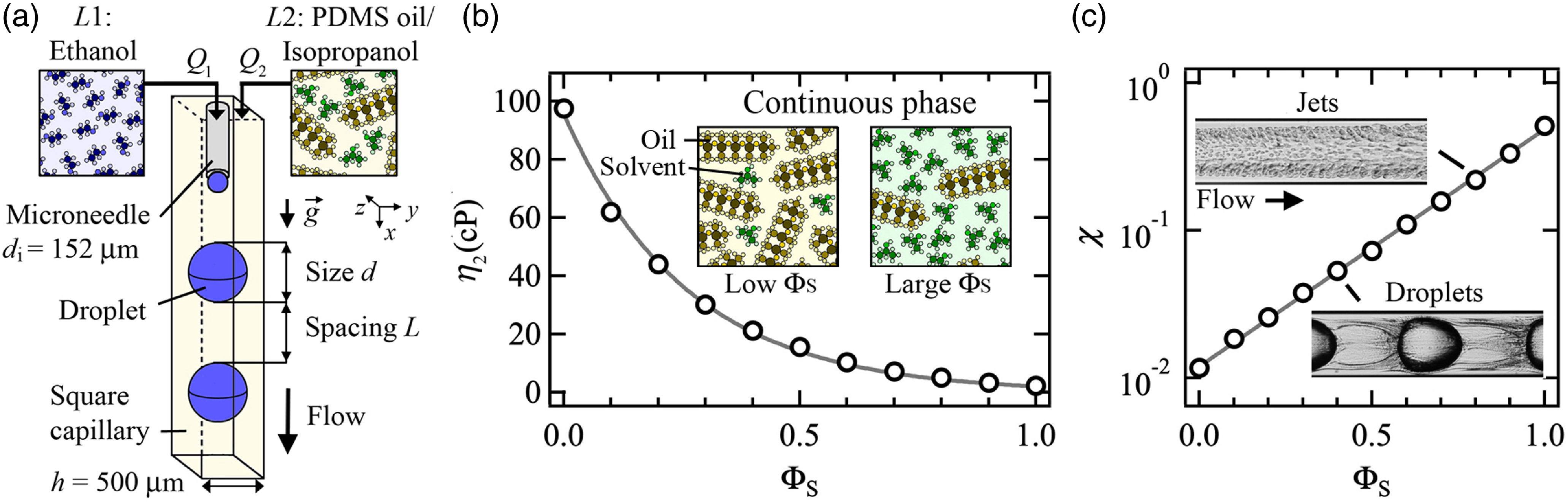
Figure 1. (a) Schematics of coaxial microchannel with fluid injection scheme, including ethanol for L1 and a mixture of oil/isopropanol for L2. (b) Measurement of dynamic viscosity η of solvent–oil mixture as a function of solvent concentration ΦS. Solid line: η 2 = 94.5exp(–3.7ΦS) cP. Inset: schematics of mixture molecular structure at low and large ΦS. (c) Evolution of viscosity ratio χ with solvent concentration ΦS. Solid line: χ = 1.2 × 10⁻² exp(3.7ΦS). Insets: micrographs of permeable (i) jets at ΦS = 0.8 and (ii) droplets at ΦS = 0.4.
To limit the influence of gravity and ensure that droplets and jets are centrally aligned with the microchannel axis at low velocities, the device is oriented vertically and downward flows are examined. In particular, periodic flows of ethanol droplets, having size d and spacing L, are observed depending on injection flow rates Q 1 and Q 2 as well as solvent concentration ΦS (figure 1(a)). The characteristics lengths, d and L, are measured through digital image processing of regular flow movies and averaged over multiple periods of droplet emission. The volumetric solvent concentration of the continuous phase, defined as ΦS = V S/(V O + V S), where V S is the solvent volume and V O is the oil volume, is varied between 0 and 0.8 to examine the cross-over between immiscible-like fluids at low ΦS and miscible-like flows at high ΦS. Silicone oil and isopropanol are mixed at room temperature with a stirrer at 1,200 rpm for approximately ten minutes in a tightly closed container to avoid hygroscopic effects, which could modify mixture turbidity and phase equilibrium, before each experiment. Optical variations of multiphase flows are observed depending on camera focus and lenses at various ΦS. We measure the viscosity of a homogeneous mixture of oil and solvent as a function of ΦS using viscometer tubes and the function η 2 = 94.5exp(–3.7ΦS) cP for calculating the dynamic viscosity of the mixture is in good agreement with data (figure 1(b)). The significant change in mixture viscosity results in a variation of the viscosity ratio χ = η 1/η 2 between the central and external phase of multiphase flows ranging from 10–2 at low ΦS to 5 × 10⁻¹ at large ΦS (figure 1(c)).
3. Flow regimes
We systematically examine microflow arrangements as a function of flow rates, Q 1 and Q 2, for various solvent concentrations ΦS (figure 2(a)). While a wide range of flow morphologies are obtained from the beginning to the end of microchannels, three main types of regimes are identified in the field of view near the fluid contactor, ranging from x = 0 at the needle tip to approximately x/h ∼ 10, including (a) droplet flow patterns, which comprise the dripping regime, where droplets form from a growing meniscus of L1 at the tip of the microneedle, and the jetting regime, where droplets are emitted at the tip of a slender jet of L1 (figure 2(c)), (b) wetting and phase inversion flow regimes, where dynamic wetting leads to the encapsulation of L2 or the formation of complex stratifications at the walls (figure 2(b)) and (c) jet regimes, which are characterised by various core–annular flow patterns (figure 2(d)]). Such generic flow regimes are also observed for pure fluids at ΦS = 0 with notably wetting regimes found at low Q 2 and jet regimes obtained at large Q 1. Initially continuous jets eventually breakup into droplets due to the Rayleigh–Plateau instability, however, due to the convective nature of the instability, at large injection velocities, jets remain locally stable and form continuous streams over distances x/h>10 that are of the order of the typical size of microfluidic systems.
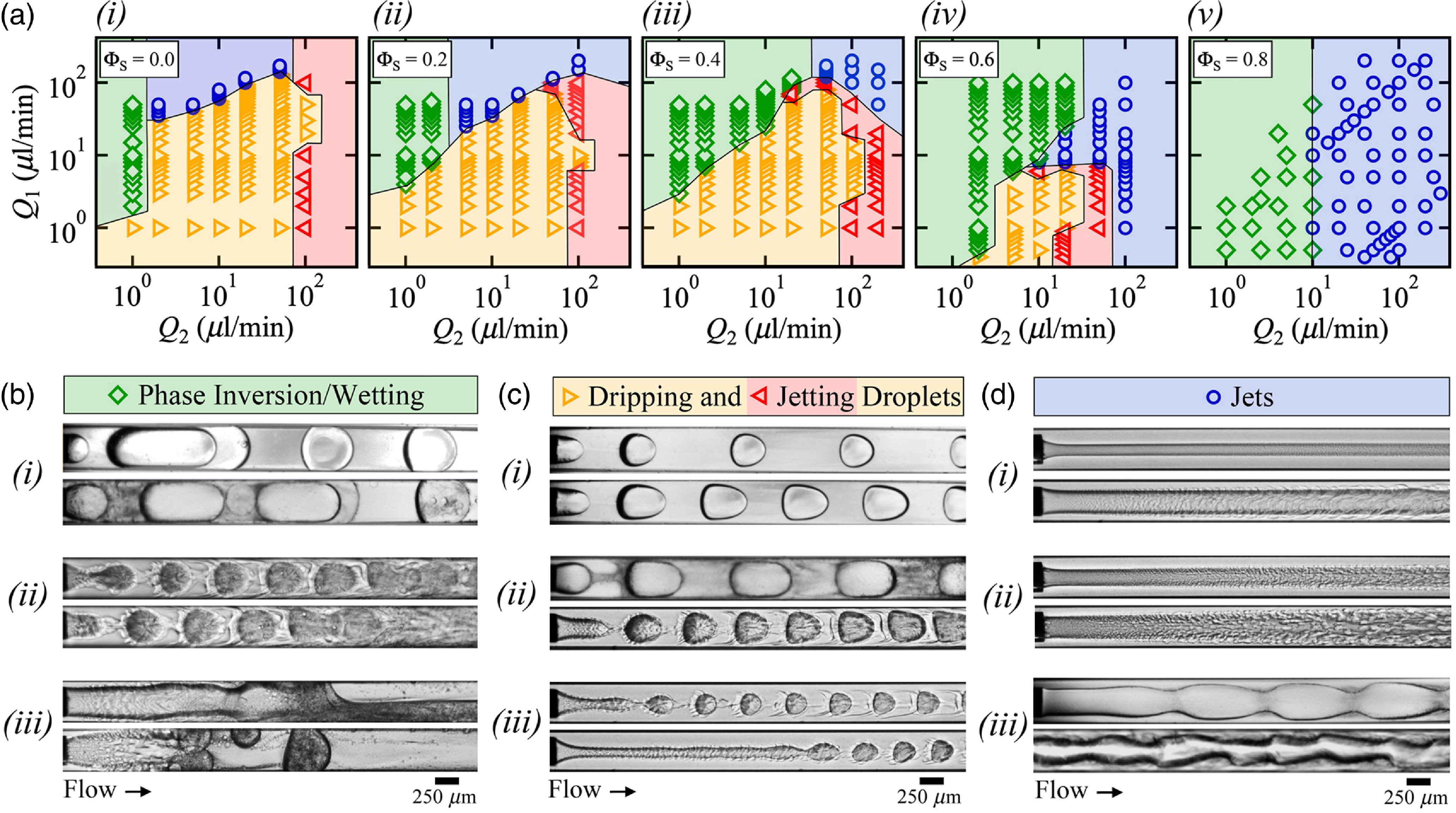
Figure 2. (a) Maps of flow regimes based on injection rates Q 1 and Q 2, including dripping(![]() ), jetting(
), jetting(![]() ), phase inversion(
), phase inversion(![]() )and core–annular flows(
)and core–annular flows(![]() ), at various solvent concentrations (i) ΦS = 0.0, (ii) 0.2, (iii) 0.4, (iv) 0.6 and (v) 0.8. (b, c and d) micrographs of typical flow regimes, flow rates in μl/min, from top to bottom. (b) Phase inversion/wetting regime: (i) phase inversion of large droplets (ΦS, Q 1, Q 2) = (0.0, 2, 1) and (0.4, 1, 1), (ii) wall coalescence of small droplets (0.6, 0.6, 5) and (0.6, 0.9, 5) and (iii) wetting jets (0.6, 40, 10) and (0.8, 0.5, 2). (c) Dripping and jetting droplets regimes, (i) dripping droplets at low ΦS (ΦS, Q 1, Q 2) = (0.0, 2, 10) and (0.0, 6, 10), (ii) dripping droplets at moderate ΦS (0.4, 3, 5) and (0.6, 4, 20) and (iii) jetting droplets (0.6, 1, 20) and (0.6, 3, 50). (d) Jet regimes, (i) quasi-straight jets (ΦS, Q 1, Q 2) = (0.8, 20, 200) and (0.6, 50, 50), (ii) swelling jets (0.8, 0.5, 50) and (0.8, 0,2, 20) and (iii) varicose jets (0.4, 170, 50) and (0.6, 15, 50).
), at various solvent concentrations (i) ΦS = 0.0, (ii) 0.2, (iii) 0.4, (iv) 0.6 and (v) 0.8. (b, c and d) micrographs of typical flow regimes, flow rates in μl/min, from top to bottom. (b) Phase inversion/wetting regime: (i) phase inversion of large droplets (ΦS, Q 1, Q 2) = (0.0, 2, 1) and (0.4, 1, 1), (ii) wall coalescence of small droplets (0.6, 0.6, 5) and (0.6, 0.9, 5) and (iii) wetting jets (0.6, 40, 10) and (0.8, 0.5, 2). (c) Dripping and jetting droplets regimes, (i) dripping droplets at low ΦS (ΦS, Q 1, Q 2) = (0.0, 2, 10) and (0.0, 6, 10), (ii) dripping droplets at moderate ΦS (0.4, 3, 5) and (0.6, 4, 20) and (iii) jetting droplets (0.6, 1, 20) and (0.6, 3, 50). (d) Jet regimes, (i) quasi-straight jets (ΦS, Q 1, Q 2) = (0.8, 20, 200) and (0.6, 50, 50), (ii) swelling jets (0.8, 0.5, 50) and (0.8, 0,2, 20) and (iii) varicose jets (0.4, 170, 50) and (0.6, 15, 50).
Overall, the main influence of solvent concentration ΦS on flow maps is to reduce the operating range of droplet dispensation regimes, which progressively shift from nearly full range at ΦS = 0 (figure 2(a)(i)) to null at large ΦS = 0.8 (figure 2(a)(v)). While dripping flows are readily produced for purely immiscible fluids at ΦS = 0 (figures 2(c)(i)), the oil–solvent continuous phase becomes progressively turbid due to the spontaneous emulsification of a diffusive fluid layer — referred to as conjugate or consolute fluid layer — around microfluidic droplets, which recirculate in segmented flows as ΦS increases (figure 2(c)(ii)). At moderate ΦS = 0.6, dripping flows consists of compact arrangements of droplets evolving in time in a sheath of conjugate fluids and significant shifts toward lower values of flow rates are observed for both the droplet/jet regime transition as well as for the dripping/jetting transition. Previous work on multiphase flow in microchannels have highlighted the importance of the capillary number Ca = ηJ/γ, where η is the dynamic viscosity and the velocity J = (Q 1 + Q 2)/h 2, on transition between dispersed and separated flows (Hu & Cubaud, Reference Hu and Cubaud2020). Here, the dripping/jetting transition at low Q 1 occurs around Q 2 ∼ 102 μl/min–1 for low ΦS between 0 and 0.4 but decreases to 2 × 101 μl/min–1 at moderate ΦS = 0.6 and disappears at large ΦS = 0.8, which suggests that the interfacial tension γ remains relatively constant at low ΦS and sharply diminishes at moderate ΦS before vanishing at large ΦS. A similar behaviour is observed for the droplet/jetting transition at large Q 1 with a steep decrease of approximately an order of magnitude in critical Q 1 between ΦS = 0.4 and 0.6 (figure 2(a)(iv)]). The morphological evolution of droplet flows based on solvent concentration is examined in the next section.
At low velocities, another regime of interest consists of the partial wetting of ethanol droplets and jets at the walls of microchannels made of borosilicate glass. Dynamic wetting properties typically induce the phase inversion of liquid–liquid dispersions with the generation of solvent-rich oil L2 droplet in a continuous phase of ethanol L1 (figure 2(b)(i)). As ΦS increases, significant mass transfer across the interface results in the rupture of the intercalating film of L2 between walls and droplets with the formation of complex stratifications with spontaneous emulsification at the walls (figure 2(b)(ii)). This phenomenon is also observed during the formation of jets at high ΦS (figure 2(b)(iii)).
Finally, continuous separated flows are generally obtained at large velocities with a variety of core–annular flow patterns resulting, including straight jets (figure 2(d)(i)), swelling jets (figure 2(d)(ii)) as well as varicose and distorted jets (figure 2(d)(iii)). Strongly diffusive jets are found to enlarge in sheaths of spatially developing layers of emulsifying conjugate fluids with the formation of periodic structures at high ΦS. In the following, we study the evolution of the three main regimes, including droplet, phase inversion and jet flow patterns.
4. Droplets
We first examine the evolution of quantities associated with immiscible multiphase flows made of ethanol and pure oil, i.e. at null solvent concentration ΦS = 0. In particular, the streamwise length of droplets d/h is measured in the dripping and jetting regimes at fixed side flow rate Q 2 and varying central flow rate Q 1 (figure 3(a)). For large droplets, the size is found to scale as φ = Q 1/Q 2 according to
 \begin{equation}d/h=k_{\rm D} \varphi,\end{equation}
where the constant k D = 0.97, as expected from the typical dripping regime of immiscible flows at low χ « 1 (Hu & Cubaud, Reference Hu and Cubaud2020). By contrast, for small sizes d/h<1, the scaling of jetting flow is recovered, such as
 \begin{equation}d/h= k_j\varphi ^{1/3}, \end{equation}
with k J = 1.15. The distinction between dripping and jetting regimes is not so sharp for very small droplet sizes, which follow a similar scaling, as can be seen in figure 3(b) for low φ. Overall, while small variations of d/h are observed based on flow velocity Q T/h 2, the droplet size remains largely independent of flow velocity for ΦS = 0. In comparison with d/h, the spacing between droplets L/h is found to mainly depends on flow rate Q 1 at large values and φ at lower values. In particular, data show that the spacing decreases according to L/h ∼ Q 1–1/2 (figure 3(c)). A useful parameter of segmented flows is the wavelength λ = d + L of droplet patterns, which reaches a minimum value at the transition between diluted and concentrated flows (figure 3(d)). The lowest value of λ also marks the transitions in scaling laws between d/h ∼ φ 1/3 and d/h ∼ φ. For diluted flows, the wavelength of repeating units of segmented flows is strongly dominated by the droplet size d/h, whereas λ is controlled by L/h. Hence, the normalised wavelength scales as λ/h ∼ φ for large φ (figure 3(e)) and λ/h ∼ Q –1/3 for low φ (figure 3(f)). In both cases, various iso-Q 2 branches of λ/h are observed in graphs with a reduction of the wavelength as the side flow rate Q 2 increases. At larger Q 2, the transition to the jetting morphology with low values of both d and L is found to follow
 \begin{equation}\lambda / h= k_{\mathrm {L}} \varphi ^{1/6}, \end{equation}
where k L = 1.6 as well as the scaling relationship λ/h ∼ Q 11/6. Overall, these relationships, obtained for pure fluid pairs in the absence of mass transfer across the interface provide a useful metric to characterise droplet formation at low χ in coaxial microchannels.
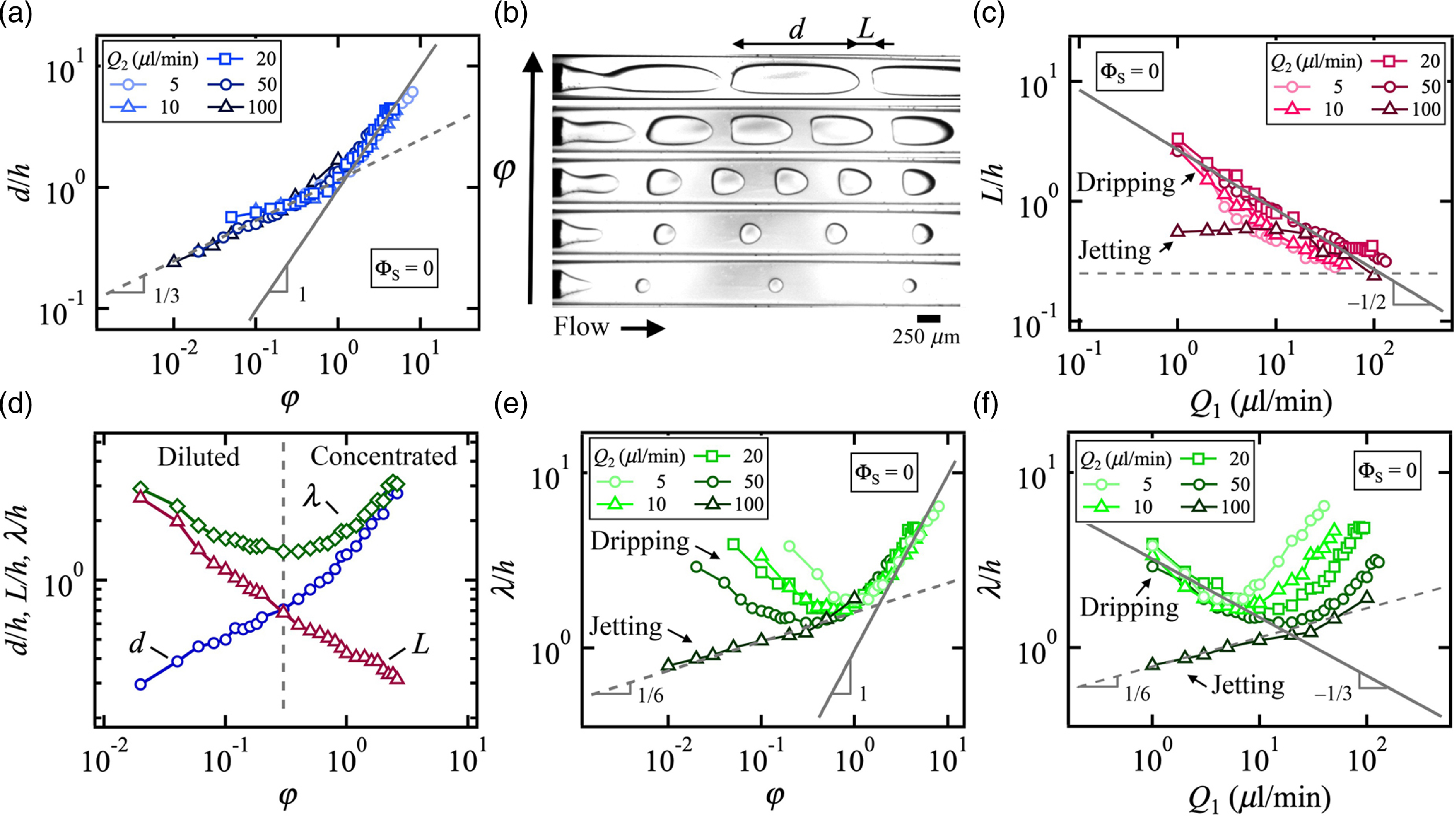
Figure 3. Reference segmented flow with pure fluids at ΦS = 0. (a) Evolution of droplet size d/h with flow rate ratio φ. Solid line: Eq. (4.1). Dashed-line: Eq. (4.2). (b) Micrographs of ethanol droplet formation in pure oil at fixed Q 2 = 50 μl/min, from bottom to top: Q 1 = 1, 3, 15, 50, 130 μl/min. (c) Droplet spacing L/h as a function of inner phase flow rate Q 1. Solid line: L/h = 2.7 Q 1–1/2. Dashed line: L/h = 0.25. (d) Variations of segmented flow wavelength λ/h with φ based on d/h and L/h at fixed Q 2 = 50 μl/min and varying Q 1. (e) Normalised wavelength λ/h versus flow rate ratio φ. Solid line: λ/h = 0.97φ. Dashed line: λ/h = 1.6φ 1/6. (f) Evolution of λ/h with Q 1. Solid line: λ/h = 3.2Q1–1/3. Dashed line: λ/h = 0.78Q11/6.
We now turn our attention to the role of the solvent concentration ΦS on droplet morphology and examine the evolution of d/h in the diluted regime at low φ. In general, the droplet size is found to slightly increase with ΦS and follows Eq. (4.2) similar to that of the pure oil case, where k J depends on both ΦS and the side flow rate Q 2 as shown in figures 4(a) to 4(c). Data for each iso-Q 2 curve is fitted with the previous equation and values of the measured factor k J are plotted for each ΦS as a function Q 2 (figure 4(d)). While a small dependence on Q 2 is found according to k J = k 0Q 2–0.15, the dimensional prefactor k 0 is well fit with a restricted equation of the form k 0 = 1.8ΦS0.87 (figure 4(d)-inset). The overall increase in droplet size d/h at low velocities is expected from the reduction in capillary number albeit this is not significant at ΦS = 0 over the range of parameters investigated in this work. Despite the complexity in the evolution of droplet flows in a solvent-rich oil phase, the change in initial droplet size remains relatively modest as ΦS increases. At moderate concentration ΦS = 0.4, the continuous phase becomes progressively cloudy due to the interdiffusion of solvent and ethanol across the droplet interface and observations of fine dispersions in the continuous phase at low velocities suggest the presence of a flux of ethanol from droplets into the external phase, which is driven by large solvent concentration near the interface (figure 4(e)). Over time, streams of miniature droplets coalesce into bigger droplets as can be seen in figure 4(e), downstream of the reference droplet at longer times. While the continuous phase morphology spatially evolves at modest ΦS = 0.4, segmented flow characteristics, such d/h, L/h and λ/h, remain relatively constant along the flow direction. At larger concentration ΦS = 0.6, however, significant droplet size d/h enlargement and spacing L/h reduction are uncovered along the flow direction. To illustrate this behaviour, segmented flow features are compared for identical values of flow rates in figures 4(f) and 4(g) for ΦS = 0.4 and 0.6. At larger solvent concentration, it is found that, while d/h and L/h vary along the flow direction, the wavelength of segmented λ/h remains essentially constant (figure 4(h)). In this case, droplet growth indicates a flux of solvent from the continuous phase to the droplet, which is accompanied by a drastic modifications of the morphology of flow pattern unit cells, having a fixed spatial period.
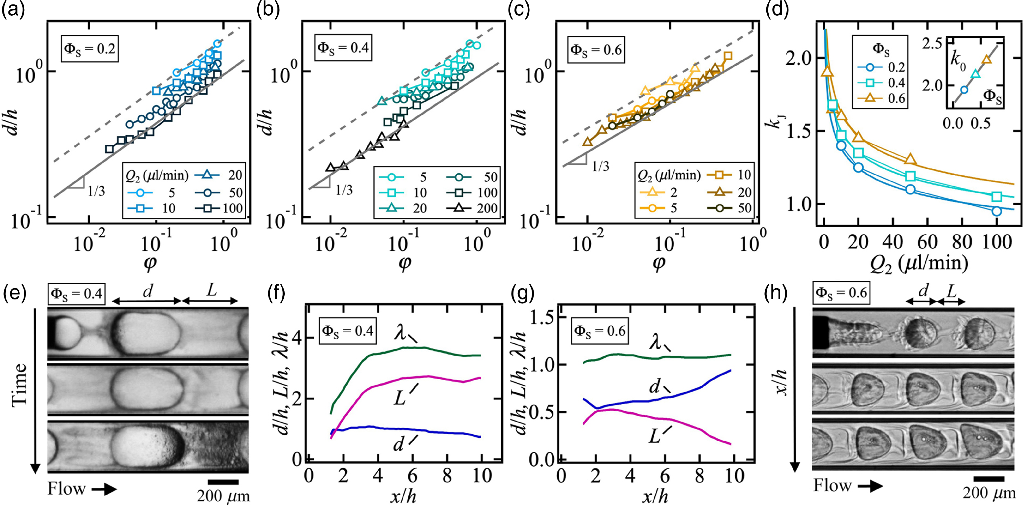
Figure 4. Droplet formation at low φ. Flow rates in μl/min. (a) Evolution of d/h as a function of φ for ΦS = 0.2. Solid line: d/h = 0.95φ 1/3. Dashed- ine: d/h = 1.67φ 1/3. (b) Variation of droplet size with flow rate ratio for ΦS = 0.4. Solid line: d/h = 0.91φ 1/3. Dashed line: d/h = 1.68φ 1/3. (c) Droplet size d/h versus φ for ΦS = 0.6. Solid line: d/h = 1.3φ 1/3. Dashed line: d/h = 1.9φ 1/3. (d) Role of flow rate Q 2 on prefactor kJ for ΦS = 0.2(![]() ), 0.4(
), 0.4(![]() )and 0.6(
)and 0.6(![]() ).Solid lines: k J = k 0Q 2–0.15. Inset: k 0 versus ΦS. Solid line: k 0 = 1.8ΦS0.87. (e) Time series of micrographs in the droplet reference frame at ΦS = 0.4 for (Q 1, Q 2) = (3, 5), Δt = 2 s. (f) Spatial evolution of d/h, L/h, and λ/h at ΦS = 0.4 for (Q 1, Q 2) = (1, 10). (g) Flow spatial evolution at ΦS = 0.6 for (Q 1, Q 2) = (1, 10). (h) Micrograph showing spatial evolution of droplet microflows at ΦS = 0.6 for (Q1, Q2) = (1, 10), Δx/h ∼ 3.
).Solid lines: k J = k 0Q 2–0.15. Inset: k 0 versus ΦS. Solid line: k 0 = 1.8ΦS0.87. (e) Time series of micrographs in the droplet reference frame at ΦS = 0.4 for (Q 1, Q 2) = (3, 5), Δt = 2 s. (f) Spatial evolution of d/h, L/h, and λ/h at ΦS = 0.4 for (Q 1, Q 2) = (1, 10). (g) Flow spatial evolution at ΦS = 0.6 for (Q 1, Q 2) = (1, 10). (h) Micrograph showing spatial evolution of droplet microflows at ΦS = 0.6 for (Q1, Q2) = (1, 10), Δx/h ∼ 3.
As the wavelength of flow patterns remains spatially constant at low and large concentrations, the parameter λ/h provides a useful metric to examine multiphase flows. From small to moderate ΦS = 0.2 and 0.4, the spatial period of regular patterns of dripping droplets follows a very similar behaviour as that of the pure fluid case at ΦS = 0, with scaling laws such as λ/h ∼ φ at large φ and λ/h ∼ Q 1–1/3 at low velocities, as displayed with solid lines in figures 5(a) and (b). Likewise, Eq. (4.3) associated with the wavelength of jetting droplets is recovered, namely λ/h ∼ φ 1/6 with similar prefactors k L as for ΦS = 0 and λ/h ∼ Q 11/6. For the case of large concentrations, including ΦS = 0.6, however, data for both dripping and jetting droplets collapse onto a curve defined as λ/h ∼ φ 1/6 and the wavelength is seen to decrease with side flow rates Q 2 in figure 5(c), which is contrast with observed behaviour at low ΦS as illustrated in figure 5(d)(i), where λ/h remains constant at varying Q 2 for ΦS = 0.4, and in figure 5(d)(ii), where λ/h decreases with Q 2 for ΦS = 0.6. While iso-Q 2 curves of wavelength λ/h plotted as a function of Q 1 scale with exponent 1/6, the prefactors k L in Eq. (4.3) are larger than the ones for jetting in the pure fluid case, which is indicated with a dashed line in figure 5(c) — bottom, and shown in figure 5(d)(iii). Therefore, segmented flows at large ΦS display peculiar behaviours with the formation of apparent dripping droplets adopting the behaviour of jetting droplets as a result of the solvent–droplet exchange process. The significant mass transfer occurring during droplet growth and detachment from the microneedle, with a large accumulation of solvent in the aqueous phase and a relatively slow infusion of L1 into the area with high solvent concentration around the droplet, leads to the formation of dripping flows having small droplet spacing L/h and uniform size d/h ∼ 1. As previously shown from the spatial evolution of droplets, the spacing L/h is further reduced downstream due to the recirculation of the solvent-rich phase through forced convection rolls during transport between droplets. Hence, the overall effect of solvent is the reduction of droplet spacing L/h and as a result λ/h compared with the regular dripping case. Therefore, the morphology of flows observed at low φ ∼ O( –1) resembles those expected at large flow rate ratio φ ∼ O(0) where d ∼ L, as seen in figure 5(d)(ii).
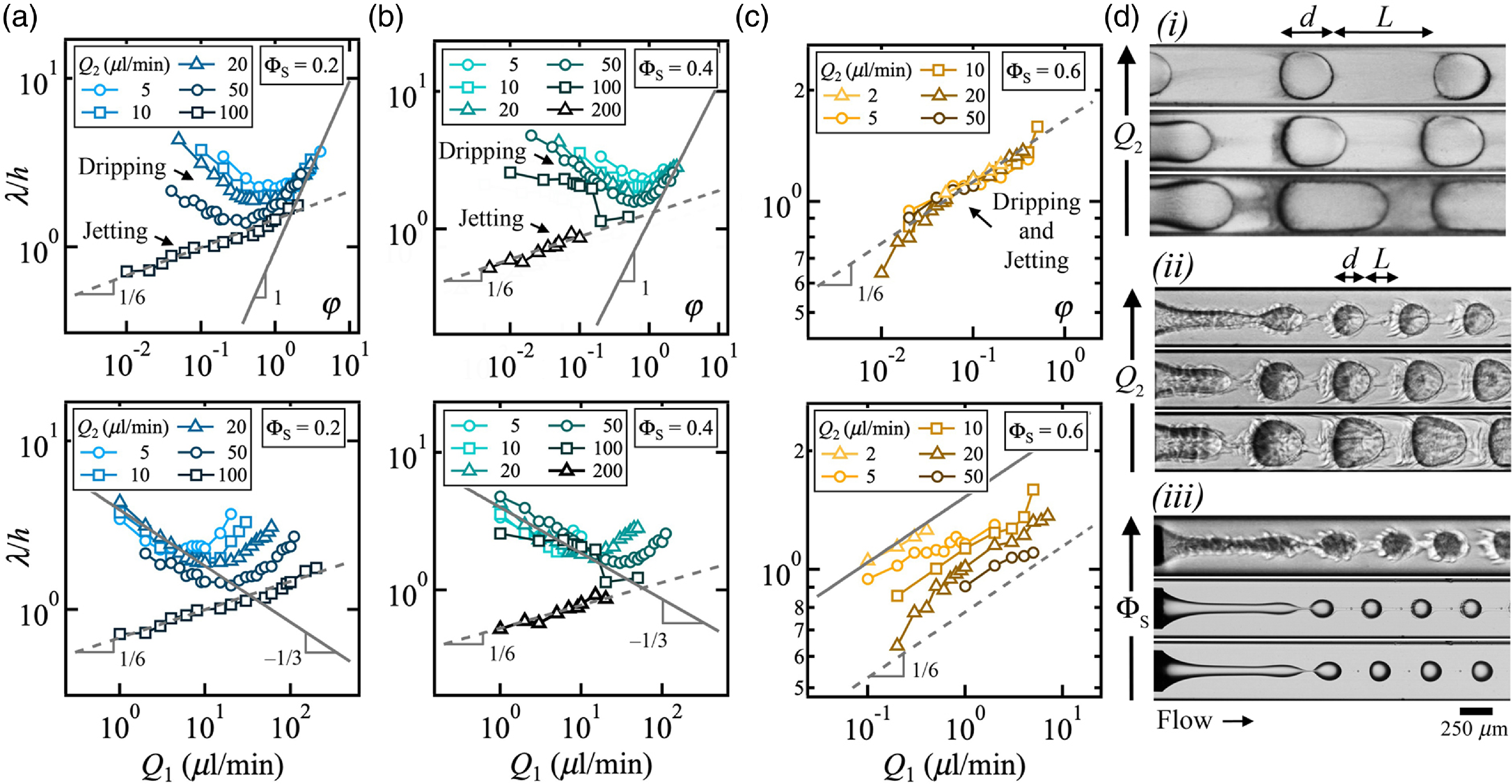
Figure 5. Characteristics of segmented flows at various solvent concentration ΦS. (a) Evolution of wavelength λ/h as a function φ and Q 1 at ΦS = 0.2. Top: solid line, λ/h = 0.97φ; dashed line, λ/h = 1.46φ 1/6. Bottom: solid line, λ/h = 3.2Q 1–1/3; dashed line, λ/h = 0.68Q 11/6. (b) Wavelength λ/h versus φ and Q 1 at ΦS = 0.4. Top: solid line, λ/h = 1.15φ; dashed line, λ/h = 1.3φ 1/6. Bottom: solid line, λ/h = 4Q 1–1/3; dashed line, λ/h = 0.53Q 11/6. (c) Variations of λ/h with φ and Q 1 at ΦS = 0.6. Top: dashed line, λ/h = 1.66φ 1/6. Bottom: solid line: λ/h = 1.53Q 11/6; dashed line: λ/h = 0.78Q 11/6. (d) Experimental micrographs. Flow rates in μl/min. (i) Role of Q 2 for ΦS = 0.4, from bottom to top (Q 1, Q 2) = (4, 5), (4, 10) and (4, 20). (ii) Role of Q 2 for ΦS = 0.6, from bottom to top (Q 1, Q 2) = (1, 5), (1, 10) and (1, 20). (iii) Jetting morphology at φ ∼ 3 × 10⁻³ , from bottom to top, (ΦS, Q 1, Q 2) = (0.2 , 3, 100), (0.4 , 7, 200) and (0.6, 0.6, 20).
The reduction of initial droplet spacing L/h as the solvent concentration ΦS increases is due in part to the combination of mass exchange between internal and external phases as well as the change of viscosity contrasts and local interfacial tension as fluids partially mix. In turn, modifications of the ratio between viscous and interfacial tension stresses during droplet formation lead to a change of flow morphology. As a result, a general trend consists in the sharp drop of the wavelength λ/h with ΦS at low φ when d/h ∼ 1, as illustrated in figure 6(a) for identical flow rates Q 1 = 1 and Q 2 = 5 μl/min across all fluid pairs. Corresponding micrographs are displayed in figure 6(b) and show the main features of solvent-infused multiphase flows investigated in this work, including a nearly immiscible two-phase flow behaviours from low ΦS = 0.2 to moderate ΦS = 0.4 with the emergence of darker streams of droplets resulting from the spontaneous emulsification of the aqueous phase in the solvent-rich oil phase at ΦS = 0.4. At larger concentrations, ΦS = 0.5 and 0.6, droplets appear surrounded by an external envelope of consolute fluids undergoing complex rearrangement processes. In addition to the influence of φ, such intriguing microstructures are also strongly dependent on absolute flow velocity Q T = Q 1 + Q 2, which sets convective time scales and residence times of droplets in the field of view. At large ΦS = 0.6, droplet flows obtained at fixed φ but various Q T show similar spatial evolution of d/h and L/h with constant λ/h (figure 6(c)) but varying temporal evolution of multiphase flows parameters (figure 6(d)). The strong dependence of the rate of deformation of d/h and L/h on absolute flow rate Q T shows the advantage of microfluidic droplet flows to enhance mass transfer with recirculating flow between droplets with segmented flows mixing faster at large velocities.
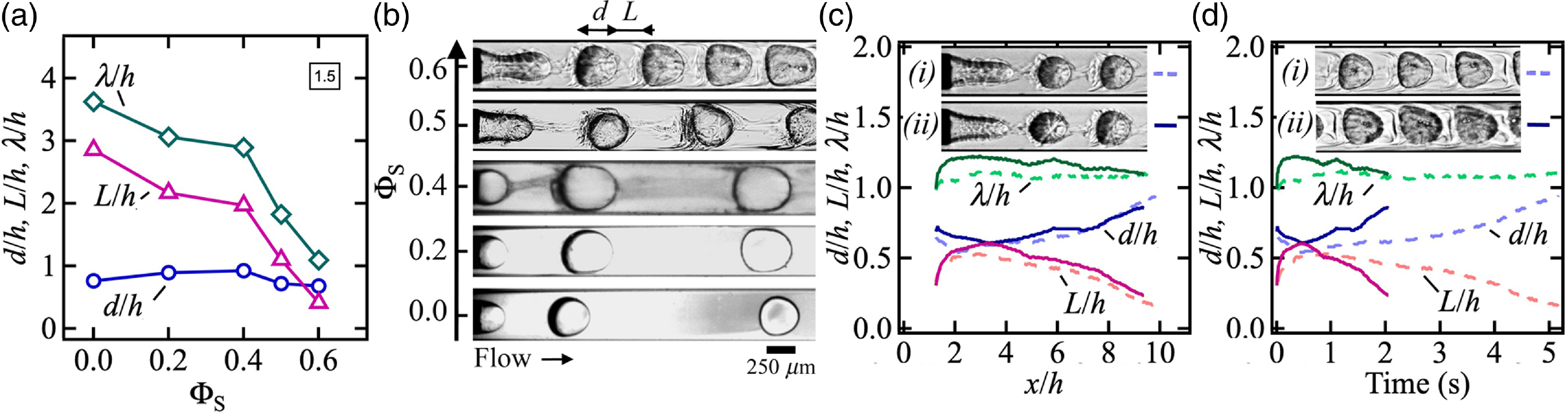
Figure 6. Morphology of segmented flows. Flow rates in μl/min. (a) Role of solvent concentration ΦS in cell characteristics, including d/h, L/h and λ/h, at fixed (Q 1, Q 2)= (1, 5). (b) Micrographs of droplet formation at (Q 1, Q 2)= (1, 5) at various ΦS. (c) Spatial evolution of flow pattern characteristic at ΦS = 0.6 and φ = 10–1 (i) Dashed lines: (Q 1, Q 2)= (1, 10); (ii) solid lines: (Q 1, Q 2)= (2, 20). Inset: micrographs of (i) and (ii) at x/h ∼ 2. (d) Temporal evolution of d/h, L/h and λ/h at ΦS = 0.6 for (i) (Q 1, Q 2)= (1, 10) and (ii) (Q 1, Q 2)= (2, 20). Inset: micrographs of (i) and (ii) at t ∼ 2 sec.
Overall, the role of solvent concentration on microfluidic multiphase flows is diverse and varied and each combination of flow rates and ΦS display unique, time-evolving microstructures. To gain better insights into microflows in the presence of spontaneous emulsification, we also document flow patterns with high-resolution photographs as shown in figure 7. This approach reveals the local partitioning of solvent around the meniscus with the formation of a thin, smooth film of isopropanol at the meniscus at moderate ΦS = 0.4 and the inception of complex filamentous structures at larger ΦS = 0.5 (figure 7(a)). In both cases, the solvent appears to permeate the meniscus near the microneedle and re-emerge at the meniscus tip to form a continuous stream of conjugate fluids, which envelops droplets further downstream. The permeation of solvent through the interface also leads to complex breakup processes, as shown in figure 7(b) with the formation of spiky microstructures in the interfacial neck during pinch-off at large ΦS. In the case of segmented flows with large droplet sizes d/h, figure 7(c) shows the progressive influence of solvent with significant turbidity observed at moderate ΦS = 0.4. The central stream made of consolute fluid flows at the peak velocity of parabolic flows ∼ 2.1Q T/h 2 in square channels, which is larger than the speed of droplets, typically adopts the average flow velocity ∼ Q T/h 2. As a result, the central stream recirculates between droplets and affects the stability of the intercalating fluids between L1 and the walls. In general, very fine microstructures of conjugate fluids form around droplets and lead to intricate, yet regular flow morphologies around droplets, as shown in figures 7(d) to 7(e).
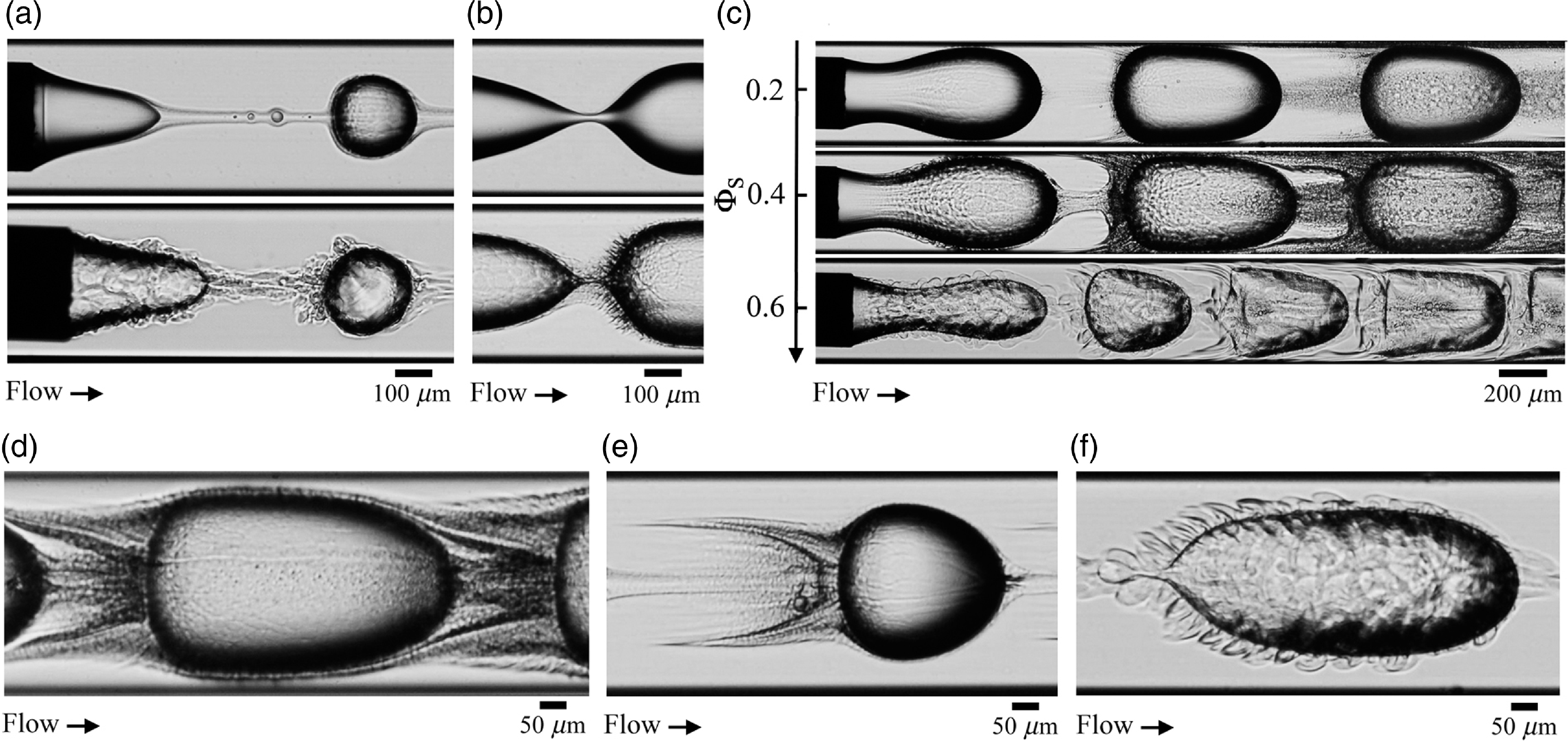
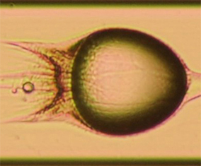
Figure 7. Photographs of microfluidic droplets in a solvent-rich oil phase. (a) Meniscus morphology at moderate ΦS = 0.4 (top) and large ΦS = 0.5 (bottom). (b) Role of solvent concentration on neck breakup, ΦS = 0.2(top) and 0.4 (bottom) with formation of conjugate fluid spikes. (c) Influence of ΦS on concentrated segmented flows. (d) Spontaneous emulsification streams around a large droplet, ΦS = 0.4. (e) Trail of consolute fluids in the wake of a small droplet, ΦS = 0.4. (f) Elongated droplets in a cloak of spiky conjugate fluids, ΦS = 0.6.
5. Phase inversion and partially wetting regimes
Another regime of interest consists of the phase inversion of segmented flows, which results from the liquid–liquid dynamic wetting properties of ethanol and silicone oil on borosilicate glass. While fully lubricated droplet flows are readily formed at large velocities Q T/h 2 and low flow rate ratios φ, i.e. for small d/h<1, partially wetting flows are observed at low Q T/h 2 and large φ. Indeed, measurements of static contact angles between ethanol droplets deposited on borosilicate glass in a bath of silicone oil show values θ E0 ∼ 300. Hence, ethanol droplets are prone to wet the hydrophilic walls of the square microchannel made of borosilicate glass at rest. As the velocity increases, however, the advancing contact angle θ E,A is expected to rise according to a Cox–Voinov relationship of the form $\theta^3_{E,A} = \theta^3_{E0} + wV$
, where w is a constant that depends on material properties (Voinov, Reference Voinov1976; Cox, Reference Cox1998). Therefore, a dynamic wetting flow transition is expected for θ E,A ∼ π above a critical velocity. Here, dynamic wetting regimes are observed at large Q 1 and low Q 2, i.e. for large droplets at small velocities, as seen in flow maps (figure 2(a)). An example of a partially wetting flow regime of droplets in coaxial microchannels is shown in the form of a time series for ΦS = 0 in figure 8(a) and the corresponding spatio-temporal diagram of the centreline is displayed in figure 8(b). This case study shows, in particular, the growth of a dewetting hole in the film of L2 between a long droplet made of L1 and the walls in figure 8(a)(ii). As L1 makes contact with the wall it encapsulates L2, which locally forms a pinching neck (figure 8(a)(iii)) that breaks to form of a partially non-wetting oil droplet having an advancing contact angle θ OA = π – θ ER, where θ ER is the receding contact angle of ethanol, and an advancing contact angle θ OR = π – θ EA. Overall, this mechanism can lead to the formation of periodic flows of oil droplets (figure 8(b)). For the case of very long droplets d/h » 1, the dynamic dewetting of the intercalating film resembles that of a bag breakup of a liquid droplet, as seen in figure 8(c). A variety of intriguing partially non-wetting flow morphologies are also observed in the presence of solvent, which induces multiphase flow inversion with the formation of spontaneously emulsifying oil droplets and solutal Marangoni flows further downstream (figures 8(d) to 8(f)).
$\theta^3_{E,A} = \theta^3_{E0} + wV$
, where w is a constant that depends on material properties (Voinov, Reference Voinov1976; Cox, Reference Cox1998). Therefore, a dynamic wetting flow transition is expected for θ E,A ∼ π above a critical velocity. Here, dynamic wetting regimes are observed at large Q 1 and low Q 2, i.e. for large droplets at small velocities, as seen in flow maps (figure 2(a)). An example of a partially wetting flow regime of droplets in coaxial microchannels is shown in the form of a time series for ΦS = 0 in figure 8(a) and the corresponding spatio-temporal diagram of the centreline is displayed in figure 8(b). This case study shows, in particular, the growth of a dewetting hole in the film of L2 between a long droplet made of L1 and the walls in figure 8(a)(ii). As L1 makes contact with the wall it encapsulates L2, which locally forms a pinching neck (figure 8(a)(iii)) that breaks to form of a partially non-wetting oil droplet having an advancing contact angle θ OA = π – θ ER, where θ ER is the receding contact angle of ethanol, and an advancing contact angle θ OR = π – θ EA. Overall, this mechanism can lead to the formation of periodic flows of oil droplets (figure 8(b)). For the case of very long droplets d/h » 1, the dynamic dewetting of the intercalating film resembles that of a bag breakup of a liquid droplet, as seen in figure 8(c). A variety of intriguing partially non-wetting flow morphologies are also observed in the presence of solvent, which induces multiphase flow inversion with the formation of spontaneously emulsifying oil droplets and solutal Marangoni flows further downstream (figures 8(d) to 8(f)).
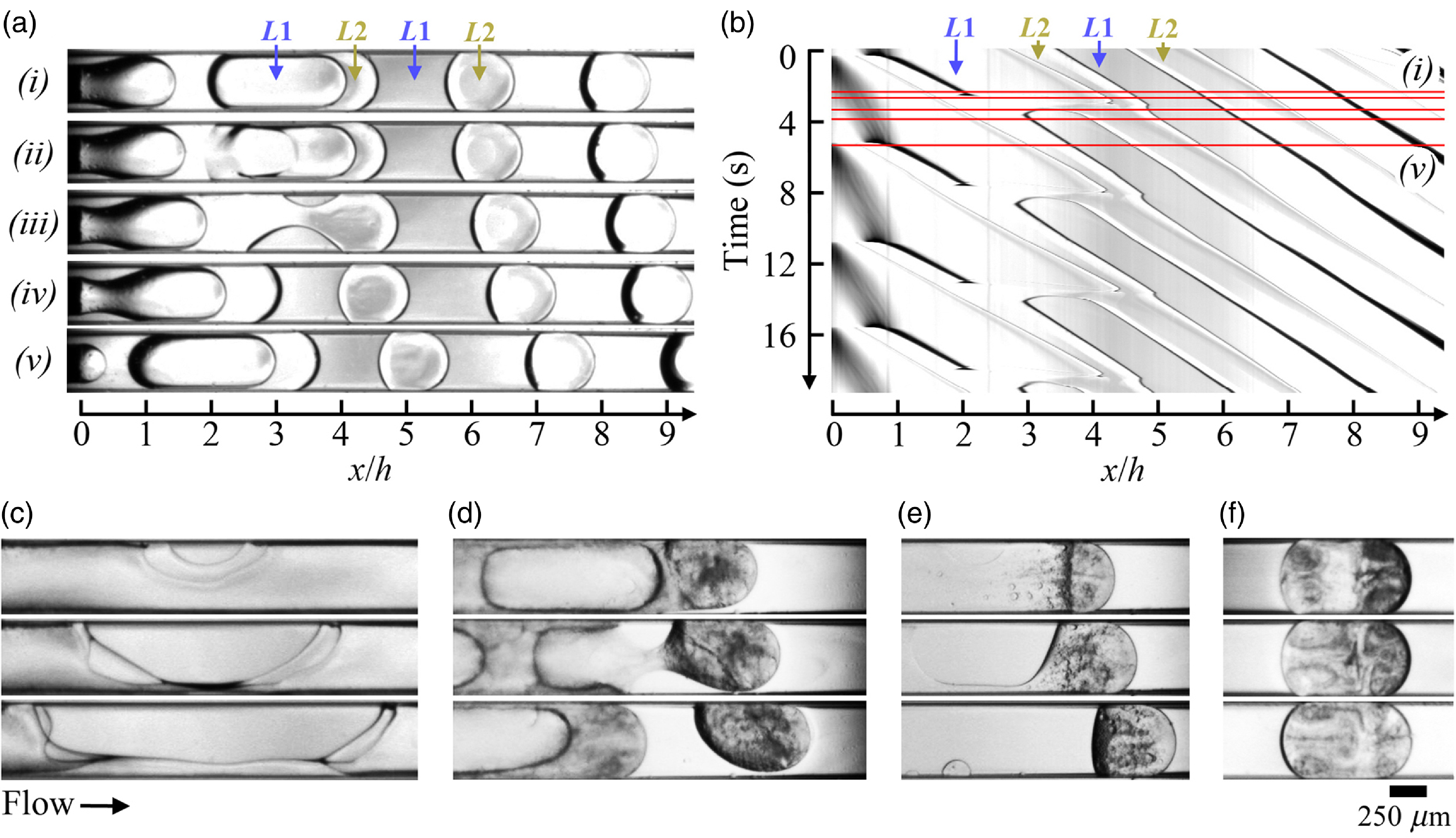
Figure 8. Dynamic wetting and phase inversion regime. Flow rates in μl/min. (a) Time series of phase inversion process due to dynamic wetting at ΦS = 0 and (Q 1, Q 2) = (2, 1). (b) Spatio-temporal diagram associated with (a). (c) Time series of dewetting hole growth resembling bag break at ΦS = 0.2, (Q 1, Q 2) = (9, 1), Δt = 3.3 × 10⁻²s. (d) Oil droplet formation at ΦS = 0.4 , (Q 1, Q 2) = (8,5), Δt = 3.3 × 10⁻¹ s . (e) Oil droplet formation at ΦS = 0.4 , (Q 1, Q 2) = (6,1) Δt = 6.7 × 10⁻¹ s. (f) Evolution of oil droplet in the droplet reference frame at ΦS = 0.2, (Q 1, Q 2) = (3, 2). Δt = 2.7 s.
6. Jets
Finally, a variety of aqueous jets are formed in a solvent-rich oil phase at very large concentration ΦS = 0.8. Core–annular flows represent an important class of separated flow pattern complementary to dispersed flow patterns made of droplets. At such large solvent concentrations, direct formation of droplets is impeded by the large solubility of the conjugate fluid layer around L1 at the fluid contactor. Hence, continuous streams of L1 are surrounded by conjugate fluids and are emitted from the cylindrical microneedle into the square microchannels at relatively large Q T. Such jets are seen to reach a minimal diameter ε M/h near the fluid contactor before enlarging due to effective diffusion with the surrounding fluids further downstream. A simple model of jet diameter ε 0/h is developed for core–annular flow based Stokes equations in circular pipes in the absence of mass transfer and interfacial tension (Cao et al. Reference Cao, Ventresca, Sreenivas and Prasad2003). In particular, the core diameter can be estimated according to
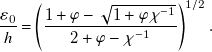 \begin{equation} \frac{\varepsilon_0 }{h}=\left(\frac{1+\varphi -\sqrt{1+\varphi \chi ^{-1}}}{2+\varphi -\chi ^{-1}}\right)^{1/2}. \end{equation}
Since for a given viscosity contrast χ = η 1/η 2, the width of the central stream is expected to depend on the flow rate ratio φ, we conduct a series of experiments at fixed φ and varying Q T to clarify the role of the absolute velocity of the flow morphology. We find, in particular, that for a given φ, ε M/h is large at low Q T and tends to ε 0/h at high Q T (figure 9(a)). Examples of flow patterns are displayed in figure 9(b) where a wide range of morphologies are observed for fixed flow rate ratio φ = Q 1/Q 2 = 2 × 10⁻² as Q T = Q 1 + Q 2 varies over two orders of magnitudes from a thin jet at large Q T to a thick core ensheathed in a layer of spontaneously emulsifying fluids at low Q T, which indicates significant mass transfer.
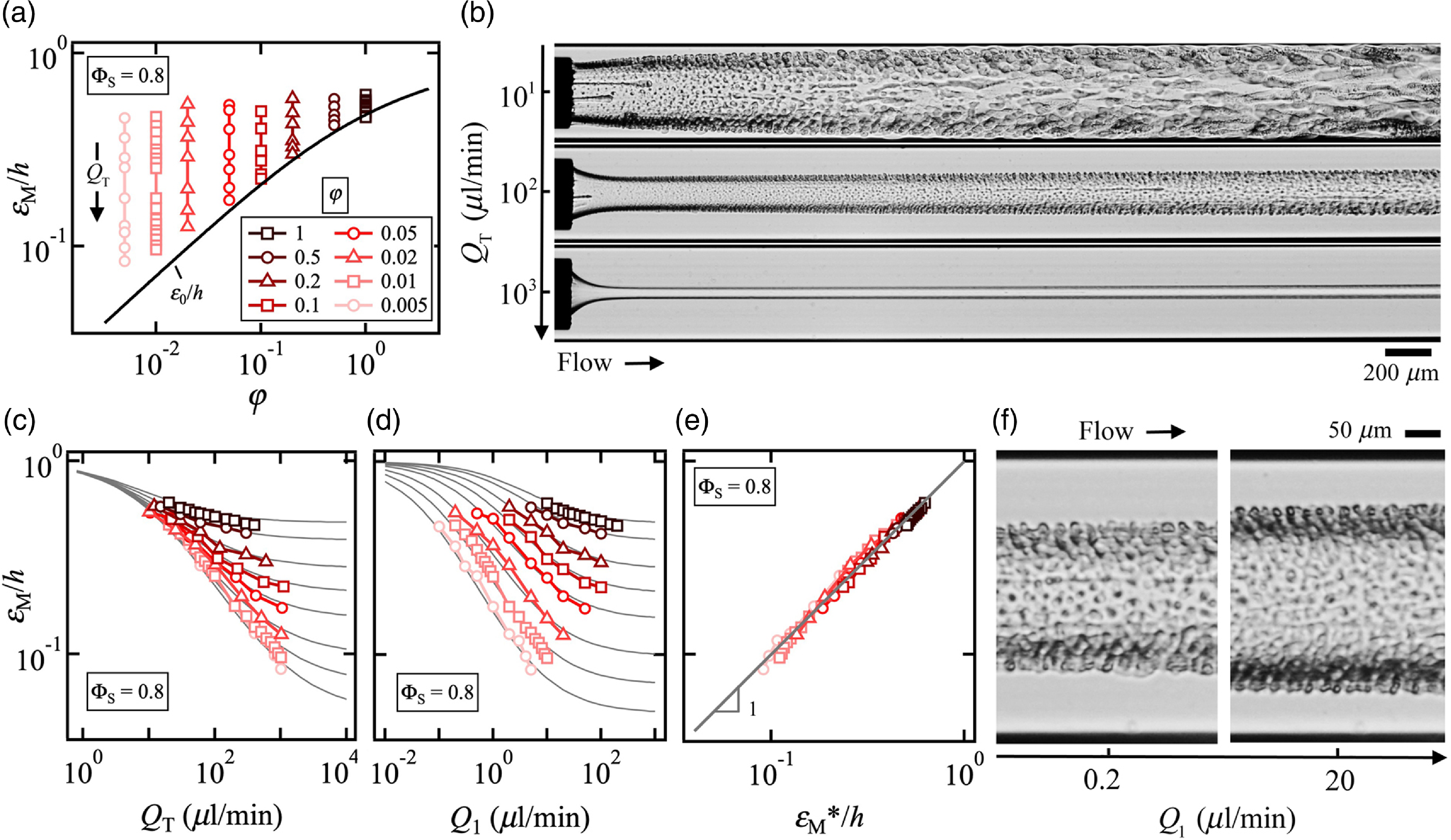
Figure 9. Formation of jets at high solvent concentration ΦS = 0.8. (a) Evolution of iso-φ curves of minimum jet diameter ε M/h as a function of flow rate ratio φ. Solid line: Eq. (6.1). (b) Micrographs showing change in flow morphology as a function of Q T for fixed φ = 2 × 10⁻². (c) Variations of iso-φ curves of ε M/h with Q T. Solid lines: Eq. 6.2. (d) Iso-φ curves of ε M/h versus central flow rate Q 1. Solid line: Eq. 6.2 with Q T = Q 1(1 + 1/φ) (e) Comparison of measured ε M/h with predicted ε M/h*. Solid line: ε M/h = ε M/h*. (f) Micrograph of jets with fixed side flow rate Q 2 = 40 μl/min and varying Q 1.
Plotting the diameter ε M/h as function of Q T reveals the strong influence of convective–diffusive phenomena with a jet diameter essentially controlled by Q T at low velocities (figure 9(c)). Since the minimum diameter ε M/h tends to unity in the highly diffusive regime at low velocities and tends to ε 0/h in the convective regime at large velocities, similar to our previous work on the stability of core–annular flows made of miscible fluids (Cubaud, Reference Cubaud2020), we model the jet evolution as function of φ and Q T using bounded functions, which find good agreement with data for the expression
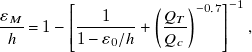 \begin{equation} \frac{\varepsilon _{M}}{h}=1-\left[\frac{1}{1-\varepsilon _{0}/h}+\left(\frac{Q_{T}}{Q_{c}}\right)^{-0.7}\right]^{-1} ,\end{equation}
where the critical flow rate Q C = 13 μl/min depends on fluid properties, including ΦS = 0.8, and the exponent –0.7 represents the steepness of curves displayed in figure 9(c). While data for ε M/h collapse onto a single curve when plotted as function of Q T a low velocities, the evolution of ε M/h for each iso-φ curves remains ungrouped when plotted as function of Q 1 as seen in figure 9(d) where fitting curves are developed based on Eq. (6.2) and the relation Q T = Q 1(1 + 1/φ). Overall, we compare measurements of ε M/h with Eq. 6.2 and find remarkable agreement with our simple phenomenological model for the jet minimum diameter, which we refer to as ε M*/h (figure 9(e)). Detailed views of jet morphology at fixed Q 2 = 40 μl/min and two widely different Q 1 = 0.2 and 20 μl/min are displayed in figure 9(f) and show the presence of periodic structures of miniature droplets of conjugate fluids at the jet interface due to the solutal Marangoni effect. Convection–diffusion phenomena are usually treated with the Péclet number Pe = Jh/D 12, where D 12 is the diffusion coefficient of the liquid pair L1/L2. Previous work on the swelling of miscible threads in microchannels has shown the similarity in critical PeC ∼ QC/(hD 12) ∼ 850 across various fluid pairs, which provides a mean for estimating D 12 ∼ Q C of swelling threads. Here, the value Q C = 13 μl/min for the composite jet at ΦS = 0.8 indicates a much larger value of effective D 12 compared with that of the mixture of 100-cSt silicone/isopropanol where Q C = 4.5 μl/min and D 12 ∼ 3.5 × 10⁻² m2s–1 (Cubaud et al. Reference Cubaud, Conry, Hu and Dinh2021). As a result, significant mass transfer is observed across the jet interface due to fast solvent shifting compared with miscible fluid diffusion. Material fluxes much larger than that due to pure molecular diffusion were also computationally observed in ternary liquid mixtures (Park et al. Reference Park, Mauri and Anderson2012).
At last, we investigate the role of solvent concentration on jet behaviour at moderate and large solvent concentrations ΦS. In particular, we examine the morphology of jets at ΦS = 0.6 at fixed values of Q 2 and various Q 1 (figure 10(a)). Similar to the previous case at ΦS = 0.8, the minimum jet diameter ε M/h is seen to tend toward ε 0/h as the flow velocity increases. We find that iso-Q 2 curves of ε M/h at ΦS = 0.6 are well fit with Eq. (6.2) using the simple identity Q T = Q 2(1 + φ) for each curve obtained at fixed Q 2 on the graph of ε M/h as a function of φ. In this case, the only fitting parameter in this family of curves corresponds to Q C = 3.6 μl/min for ΦS = 0.6. Hence, similitude arguments based on Péclet number suggest more than a threefold decrease in effective diffusion coefficient D 12 between ΦS = 0.8 and ΦS = 0.6. Examples of jet morphologies at ΦS = 0.6 are displayed in figure 10(b), where the surrounding layer of consolute fluid can be seen to develop curly structures at different jet sizes and velocities. Overall, we compare measurements of ε M/h with our phenomenological model of minimum jet diameter ε M*/h based on bounded functions and find satisfactory agreement between data and theory (figure 10(c)). We also examine the spatial evolution of jet morphology as a function of moderate and large solvent concentrations ΦS at φ = 1 for identical flow rates Q 1 = Q 2 = 100 μl/min (figure 10(d)). These micrographs show the spatial development of conjugate fluid layers ensheathing the jet at different concentrations with a nearly regular jet near the fluid contactor at moderate ΦS = 0.4, which further develop into a sparce, low-density filamentous microstructure further downstream. At medium ΦS = 0.5, the conjugate fluid layer appears to undergo a form a spinodal dewetting near the microneedle and develops into a compact, high-density filamentous structures wrapping up the jet further downstream. At large ΦS = 0.6, the conjugate fluid layer appears thicker and continuous with the development of curly microstructures further downstream. Overall, the formation of periodic and aperiodic structures made of filaments and droplets at the jet interface in the presence of solvent constitutes an intriguing topic of investigations. More work is required to fully elucidate the dynamic morphogenesis of surrounding fluid layers in ternary fluid systems based on fluid and flow properties together with Marangoni flows.
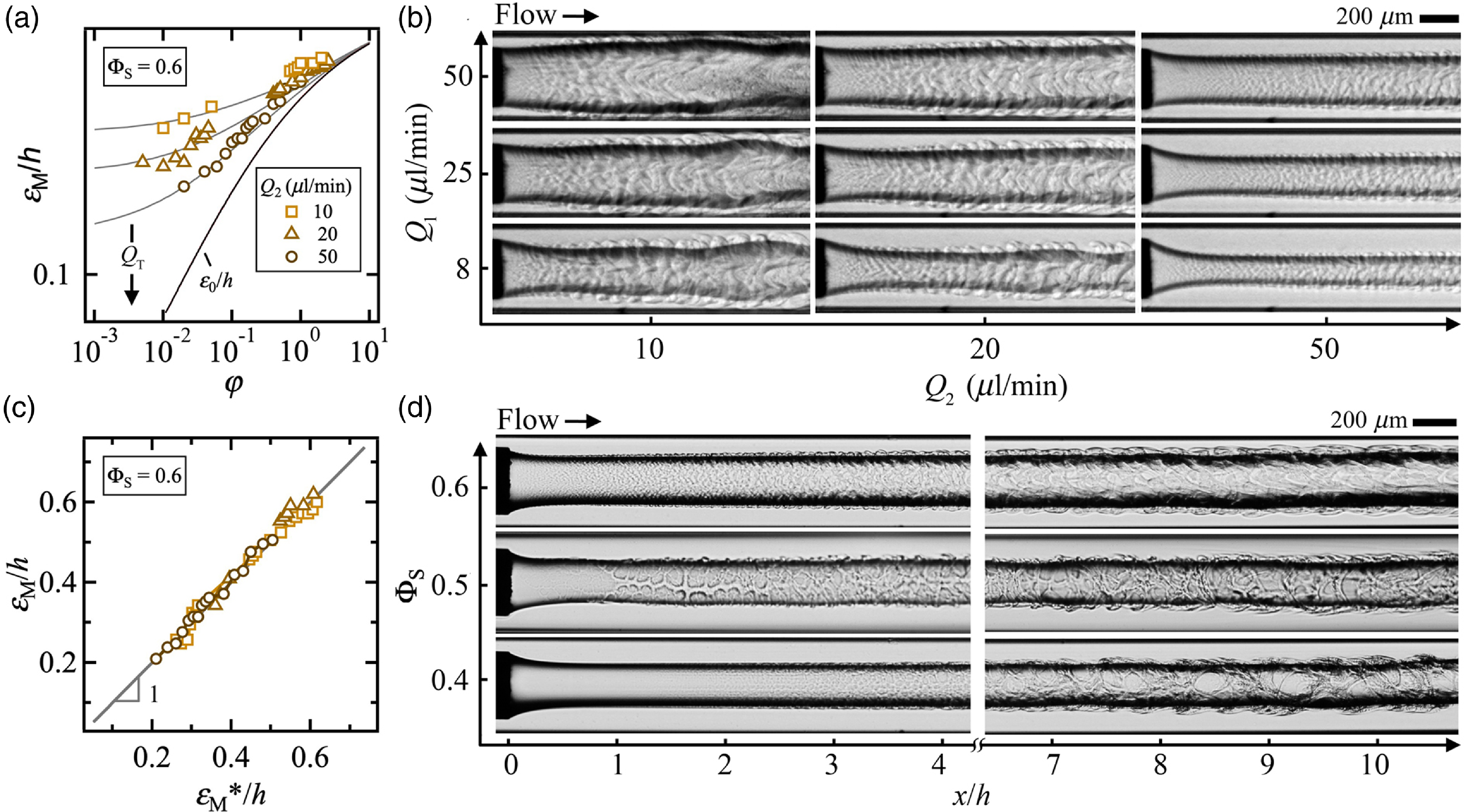
Figure 10. Jets at moderate and large solvent concentrations ΦS. (a) Evolution of iso-Q 2 curves of minimum jet diameter ε M/h as a function of flow rate ratio φ at ΦS = 0.6. Solid lines: Eq. (6.2) with Q T = Q 1 + Q 2. (b) Chart of jet micrographs near the fluid contactor at ΦS = 0.6. (c) Comparison of measured ε M/h with predicted ε M/h*. Solid line: ε M/h = ε M/h. (d) Micrograph showing the influence of solvent concentration on upstream and downstream jet morphology at φ = 1 with Q 1 = Q 2 = 100 μl/min for all fluids.
Conclusion
In this work, we experimentally investigate the two-phase flow behaviour of ternary fluid systems when a miscible solvent is preliminary blended with an oil continuous phase. We clarify the phenomenology of solvent-based immiscible flows in coaxial microchannels and unveil the presence of three main flow patterns near the fluid contactor, including droplets, jets and phase inversion. A range of intriguing droplet regimes are examined in the presence of a solvent, which progressively modifies the multiphase flow morphology and induce spontaneous emulsification of the continuous phase depending on flow rates Q 1 and Q 2 and solvent concentration ΦS. We develop scaling relationships and show that the droplet size d, spacing L and unit cell wavelength λ of segmented flows remain relatively similar from low ΦS = 0 to moderate ΦS = 0.4. At larger concentrations, significant mass-exchange processes between phases are observed with the presence of a conjugate fluid layer forming around droplets and a time-dependent evolution of flow features. It is found, in particular, that the droplet size d increases along the flow direction while the spacing L decreases. The wavelength λ of unit cells, however, remains mainly constant and follows a unique scaling with the flow rate ratio φ for both dripping and jetting droplets at large ΦS = 0.6. Comparing spatial and temporal evolutions of microfluidic droplet flows reveals mixing enhancement through forced convection of ternary fluid segmented flows due to the recirculating motion between droplets as well as the possibility to dynamically manipulate spontaneous emulsification phenomena. Another general type of flow regime is investigated at low velocities when the dispersed phase partially wets the channel walls, which results in the phase inversion of microfluidic dispersions. At large velocities, continuous separated flows are produced with the formation of a variety of core–annular flows. We analyse the evolution of the minimum jet diameter ε D/h at large solvent concentrations ΦS and show that ε D/h is controlled by the flow rate ratio φ at large velocities and mainly depends on the total flow rate Q T at low velocity. An original analysis method based on bounded functions is employed to model the evolution of jet diameters and determine a critical flow rate Q C characterising the cross-over between diffusive and convective regimes as a function of solvent concentration. We also document morphological changes in the conjugate fluid layer which develops around the central core, from a smooth film at moderate ΦS to heterogeneous filamentous structures and miniature droplets at high ΦS. Further experimental, computational and theoretical work is needed to fully elucidate the flow behaviour of droplets and jets in a solvent-rich oil phase at the small scale. Overall, this work charts new microfluidic regimes of interest for the formation of original soft material and dispersions with spontaneous emulsification phenomena using solvent additives.
Acknowledgements
We thank T. Dinh for fruitful discussions and for helping with the experimental apparatus.
Data availability
Data are available from the corresponding author (T.C.).
Author contributions
V. J. conducted experiments and data analysis at low solvent concentrations and T .C. experimentally examined large solvent concentrations. T. C. wrote the original manuscript and both authors approved the final submitted draft.
Funding
This material is based upon work supported by the National Science Foundation under Grand No. CBET-2223988.
Competing interests
None.
Ethical standards
The research meets all ethical guidelines, including adherence to the legal requirements of the study country.


 Open access