Democratic Trajectories

Every democratic regime establishes a unique trajectory – its observed evolution over time – between the transition to democracy (t = 0) and the time of its breakdown, or the last observed point in the series if the regime survived until then. Some regimes break down; others evolve toward a higher level of democracy or erode without breaking down; others experience ups and downs; many stagnate.

Trajectories characterize democratic regimes over their entire existence. Some countries experience multiple democratic regimes, and each regime has its own democratic trajectory. These trajectories are often not linear. For instance, Turkey became a democracy in 1987 and experienced a breakdown in 2014. It began with a low level of liberal democracy. Democracy gradually improved until cresting in 2004 (at 55 points on V-Dem’s Liberal Democracy index rescaled to range between 0 and 100).Footnote ¹ Then, a gradual erosion occurred from 2004 to 2012, followed by a more pronounced drop in 2013, culminating in a breakdown in 2014.

The concept of trajectories helps integrate two research traditions in the study of democracy. The quantitative tradition examines country-years as conventional units of analysis. Scholars in this tradition employ statistical models to predict the probability of regime change (democratic transitions or breakdowns) or to predict levels of democracy according to continuous measures such as those generated by Polity, Freedom House, or the V-Dem project. This approach typically conceptualizes correlates of democracy as an array of time-varying covariates with short-term effects or with long-term effects converging into a steady state. For example, econometric models establish whether an increase in income per capita in any given year is conducive to an increase in levels of democracy the following year. Dynamic panel models, which include a lagged dependent variable, allow researchers to estimate the long-term association of covariates with the outcomes of interest, assuming that some portion of that effect will carry into later periods until the level of democracy converges to a steady state (Arellano and Bond Reference Arellano and Bond1991; Ferguson and Lim Reference Ferguson and Lim2003).

The qualitative tradition usually takes country histories or specific regimes as units of analysis. Scholars in this tradition employ comparative historical analysis to explain regime outcomes over the long run – for instance, the emergence of durable democracy or recurrent dictatorship. This approach typically conceptualizes the correlates of democracy as an array of preconditions and critical junctures that determine long-term outcomes. For example, historical sociologists and political scientists seek to establish whether particular models of development in the nineteenth century undermined the possibility of democracy in the twentieth century (Mahoney Reference Mahoney2001). Theoretical assumptions in macro-comparative qualitative work about the causal chains underlying the temporal process allow for greater temporal complexity. Incremental change can have medium- or long-term effects (Pierson Reference Pierson2004) that are not captured by most models in year-to-year time series, cross-sectional datasets. As we argue later, growth curve models capture this important insight gleaned from qualitative approaches.

Our analysis of democratic trajectories engages with both traditions. Because trajectories reflect the evolution of a regime’s level of democracy over time, we can decompose them into a series of discrete time observations. Thus, we can model trajectories using econometric estimators with country-year data. At the same time, regime trajectories are more than a collection of independent data points indexed by time. Trajectories constitute our object of study at a higher level of analysis. We pursue an explanation for the trajectories’ overall shape. This goal requires that we consider preconditions that explain the initial level of democracy in the aftermath of the transition and the slope of the ensuing trend over the long run.

These two analytic traditions tend to assume two distinct types of causal processes. Democracy results from a stationary process if, in the absence of any exogenous inputs, the mean level of democracy is expected to remain stable over time. By contrast, democratization violates the assumption of stationarity if levels of democracy are expected to follow trends set by some inherited conditions or by cumulative changes in the values of the covariates.

Quantitative studies of political regimes typically rely on panel estimators that assume stationary processes. Under this assumption, empirical models can only account for democratic trajectories by decomposing them into two elements. First, some stable conditions – which can be modelled empirically or treated as unobserved fixed effects – determine the baseline level of democracy in the aftermath of the transition. Second, time-varying covariates account for any deviations from this baseline level on a yearly basis over time. Democracy is expected to improve in years when independent variables move favourably and decline in years when they change unfavourably.

This classic quantitative setup carries distinctive implications. If the effect of time-varying covariates were removed at any point in time, democracy would return to the stable equilibrium level given by time-invariant conditions. Therefore, only sustained changes experienced by trending covariates can account for democratic trajectories. Under stationary assumptions, democratic trajectories are fully reversible rather than self-sustaining. These implications suggest that standard panel models rely on implausible theoretical assumptions. As we show in the empirical section, few explanatory variables trend in parallel with regime trajectories or account for profound shifts in democracy, such as the one experienced by Turkey after 2004.

Major theories of democratization do not assume a stationary process, however, and often imply that the reversionary level of democracy shifts over time. Consider two mechanisms present in the literature. One is that the initial conditions at the time of transition affect the subsequent trajectory of democratization. For example, Albertus and Menaldo (Reference Albertus and Menaldo2018) argued that when democracies function under constitutions written under authoritarian rule, the institutional rules of the game favour ‘elite biased democracy’. In their argument, such constitutions affect the subsequent course of democratization. This example illustrates a broader class of arguments about modes of transition. Several scholars have argued that transitions engineered from above are more likely to get stuck because of the foundational concessions to the outgoing authoritarian elite (Albertus and Menaldo Reference Albertus and Menaldo2018; Fishman Reference Fishman2019; Haggard and Kaufman Reference Haggard and Kaufman2016; Hagopian Reference Hagopian1996). In these theories, initial conditions affect the subsequent course of democratization. Modelling approaches based on the assumption of stationarity fail to capture this theoretical expectation, which implies that starting conditions affect the rate of change in levels of democracy over the long run.

A second kind of argument, often implicit but rarely articulated in an explicit way, is that some time-varying covariates, such as economic growth, have cumulative effects. The implicit theoretical core of modernization arguments, for example, is not that short-term shifts in the level of development affect democracy but rather that cumulative growth creates a structural or cultural propensity for democratization. In the long term, the effects of growth crystalize into social and economic development and thereby favour democratization. Once regimes consolidate at a certain level of democracy, this threshold sets the reversion point for the next historical period. We explore this type of mechanism in greater detail in the next section.

Economic Growth and Democratic Trajectories

To illustrate the distinction between stationary processes and non-stationary processes driven by cumulative effects, we focus on the relationship between economic growth and democratic trajectories. Growth is a common predictor in empirical models of democracy. Economic performance varies considerably from year to year and thus offers a plausible explanation for democratic change within countries, as opposed to more stable variables (such as per capita GDP) that might account for more stable variations in levels of democracy across countries.

Some scholars have reported that democracies are more likely to break down during times of economic crisis (Gasioworski Reference Gasiorowski1995; Kapstein and Converse Reference Kapstein and Converse2008, 58–68; Przeworski et al. Reference Przeworski, Alvarez, Cheibub and Limongi2000). Others have reported no effect (Alemán and Yang Reference Alemán and Yang2011, 1140; Haggard and Kaufman Reference Haggard and Kaufman2016, 238–243). Still others have reported results that vary across different sets of cases (Bernhard et al. Reference Bernhard, Nordstrom and Reenock2001). However, little of the existing scholarship has looked at how cumulative growth might help establish a regime trajectory.

The most common way of modelling this relationship is to examine the association between the growth rate in one year and democracy in the next. Theoretically, however, it is not clear why economic performance in any given year would affect the political regime in the next year. If economic performance has been good over the medium to long term, most citizens would probably interpret one down year as a temporary blip. Conversely, if economic growth has been paltry over the medium to long term, there is little reason why a banner year would lead to democratic deepening. Scholars do not assume that single-year growth rates are the only way in which growth affects democracy, but this assumption is built into most models that examine this relationship.

Consider, for illustration, the historical trajectories of Argentina (1984–2017) and South Korea (1988–2017) under democracy. South Korea’s initial level of liberal democracy (42 points) was lower than Argentina’s (60 points). But South Korea had an average growth rate (4.5 per cent) much higher than Argentina’s (1.0 per cent) during this era. Over time, South Korea caught up with Argentina’s level of democracy and ended with a democratic advantage (71 versus 63). Leaving other covariates aside, a stationary process would explain the end result only if Korea’s rate of growth had been ten times greater than Argentina’s in 2017.Footnote ² But this was not the case. It is more plausible that smaller differences generated a cumulative effect.

Some studies strive to capture cumulative effects using conventional modelling strategies. For example, a few scholars have used the growth rate over a five- or ten-year average rather than a single year (for example, Kapstein and Converse Reference Kapstein and Converse2008, 58–68). Cumulative effects are also implicit in dynamic panel models, which include a lagged measure of the dependent variable because the effects of temporary interventions carry over into the long term, even though they dissipate over time. Those approaches come closer to our theoretical intuition about how economic performance affects the level of democracy, but they still assume stationarity and thus are not sufficient to capture the two mechanisms described below.

A non-stationary process may result from two plausible mechanisms.Footnote ³ The first is the ‘stickiness’ of democratic institutions, which can be represented in stylized form as an integrated series: d _t = d _t-1 + g _t, where the level of democracy at time t is determined by the level of democracy achieved in the previous period d _t-1, and by a contribution made by the level of economic growth in the current period, g _t. Assuming an initial state d ₀, the level of democracy at any point in time can be anticipated as d _t = d ₀ + ḡ*t, where ḡ is the average level of g for a series of length t.

The second plausible mechanism involves reverse causation or the possibility that democracy conditions the rate of economic growth (Acemoglu et al. Reference Acemoglu, Johnson, Robinson and Yared2008; Acemoglu et al. Reference Acemoglu, Naidu, Restrepo and Robinson2019; Przeworski et al. Reference Przeworski, Alvarez, Cheibub and Limongi2000). Consider first a standard stationary process, in which the level of democracy at time t is shaped by an initial state d ₀ and by a short-term contribution made by economic growth g _t, such that d _t = d ₀ + g _t. Nothing in this equation establishes a cumulative effect. Now, assume that economic performance is in turn shaped by the institutional context d _t-1, and by a short-term economic shock u_t, such that g _t = d _t-1 + u_t. In this case, the level of democracy at any point in time equals d _t = d ₀ (1 + t) + ū*t, where ū is the average economic shock for a series of length t.

Institutional stickiness and institutional determinants of economic growth are highly plausible assumptions, well established in the literature (Colagrossi et al. Reference Colagrossi, Rossignoli and Maggioni2020; Pierson Reference Pierson2004, Chapter 3). In both cases, the result is a cumulative process in which the average behaviour of the independent variable during the observed historical period influences the trajectory, not just the level of democracy. Under those circumstances, the mean rate of economic growth during a certain period will help account for a trajectory (that is, an upward or downward trend) in democracy scores during that period. In the empirical applications discussed in the next section, the predicted regime trajectory is given by the initial level of democracy, the ensuing trend (shaped by cumulative effects), and the year-to-year oscillations created by other factors.

This different understanding of the data-generating process leads to a focus not exclusively on year-to-year growth as conventional panel models typically assume, but also on average medium- to long-term growth. It seems theoretically intuitive that average mediocre or stellar growth over time could affect democracy. Over time, robust growth transforms social structures in ways that are likely favourable to democratic deepening. It might lower the populist temptation by generating more satisfaction with democracy because of good economic performance. Conversely, sluggish medium- to long-term average growth might make democratic deepening more difficult. It could generate citizen dissatisfaction with democracy, thereby opening the doors to populists who rail against established institutions and work to undermine them. It could also result in disappointment with democracy among some establishment actors. In this perspective, it was Venezuela’s extended and cumulatively deep economic decline over more than two decades (1977–98) rather than a short-term economic crisis that facilitated the electoral victory of populist outsider Hugo Chávez in 1998. Over time, a decisively better economic performance could help democratic deepening, and poor economic performance could hinder it. The medium to long-term rate of economic growth and other independent variables generate a trajectory for the regime. These arguments are consistent with the long tradition of qualitative analyses of democratization that have focused on medium- to long-term influences.

Modelling Regime Trajectories

We use latent growth curve models to estimate the effect of covariates on democratic trajectories. Growth curve models are not new in democracy studies (Finkel et al. Reference Finkel, Pérez-Liñán and Seligson2007; Wejnert Reference Wejnert2014), but they have an affinity with the concept of regime trajectories developed in this paper. While many users of growth curve models approach them as an instance of structural equation modelling, we approach them as an instance of hierarchical linear modelling (on the equivalence of approaches, see Chou, Bentler, and Pentz Reference Chou, Bentler and Pentz1998).

To underscore the compatibility of growth curve models with other methods, we conceptualize them as an extension of traditional ways of modelling levels of democracy, focusing on three strategies. First, conventional fixed-effects models discard cross-sectional variance and estimate coefficients exploiting temporal variance within cases. Second, hybrid panel models combine fixed-effects and random-intercept estimators to leverage variation between cases. The third strategy, random growth curve models, builds on the hybrid estimator to predict the latent trend for each regime.

We go over each estimation strategy in detail to show that the three modelling strategies are nested; simpler estimators represent constrained versions of more complex ones. While fixed-effects models focus on short-term ‘within’ effects (variance over time within countries) and hybrid models add information about ‘between’ effects (cross-sectional variance), latent growth curve models incorporate a random slope, capturing unique trajectories for each regime.

Conventional fixed-effects models remove cross-sectional variation by adding country dummies to capture unit effects on the right-hand side of the equation. An alternative estimation strategy yields the same coefficients by ‘centring’ the predictors; that is, by subtracting the unit’s average from each variable:

([1]) $${Y_{it}} = {\rm{ }}{\rm{b}_0} + {\rm{ }}{\rm{b}_1}({X_{it}}-{\bar X_i}){\rm{ }} + {u_i} + {e_{it}}$$

where Y is the level of democracy for unit (regime) ${\bar X_{\rm{i}}}$ at time t; X _it is the score for a given predictor (say, economic growth) in that unit-year, and ${\bar X_{\rm{i}}}$ is the average for the unit. For consistency in the presentation of this section, we unconventionally include u _i = Ῡ _i on the right-hand side rather than on the left-hand side of the equation (that is, Y _it – ${\bar Y_{\rm{i}}}$ ).

Fixed-effects models account for unobserved cross-sectional confounders. For example, Acemoglu et al. (Reference Acemoglu, Johnson, Robinson and Yared2008) employ them to argue that per capita income has no correlation with levels of democracy after accounting for unobserved country characteristics. Many applications also incorporate period-fixed effects (for example, dummies for each year, five-year period, or decade), but a growing literature underscores the problems of interpretation created by this approach (Kropko and Kubinec Reference Kropko and Kubinec2020). In the best scenario, two-way fixed-effects models capture parallel trends but not unique regime trajectories.Footnote ⁴ And because unit effects remove cross-sectional variation from the analysis, time-invariant predictors cannot be used as covariates.Footnote ⁵

To address these limitations, other estimators combine cross-sectional and time-varying predictors. This family of techniques includes hierarchical random-effects models (Raudenbush and Bryk Reference Raudenbush and Bryk2002), fixed-effects vector-decomposition models (Plümper and Troeger Reference Plümper and Troeger2007), correlated random effects models (Mundlak Reference Mundlak1978; Wooldridge, Reference Wooldridge2019) and hybrid effects models (Allison Reference Allison2009; Finkel Reference Finkel, Atkinson, Delamont, Cernat, Sakshaug and Williams2020). We focus on the latter, as the ‘hybrid’ estimator is an extension of fixed-effects models and a constrained version of growth curve models.

Hybrid models build on Equation 1 and incorporate the unit’s average for each predictor, Ẋ _i, to account for cross-sectional effects:

([2.1]) $${Y_{it}} = {\rm{ }}{\rm{b}_0} + {\rm{ }}{\rm{b}_1}({X_{it}}-{\bar X_i}){\rm{ }} + {\rm{ }}{\rm{b}_2}{\bar X_i} + {u_i} + {e_{it}}$$

This estimator partitions residual variance into a random unit effect (u _i) and a stochastic error (e _it). The intercept for each case is given by a unit-level equation:

([2.2]) $${\rm{b}_i} = {\rm{ }}{\rm{b}_0} + {\rm{ }}{\rm{b}_2}{\bar X_i} + {u_i},$$

and varies as a function of cross-sectional predictors.

The estimate of b₁ retrieved from Equation 2 (hybrid) is equivalent to the estimate from Equation 1 (fixed-effects) in balanced panels if both include the same predictors (Mundlak Reference Mundlak1978). But Equation 2 also allows for the inclusion of cross-sectional predictors that display no variance over time. Hybrid estimators thus provide a multi-level strategy to assess the effect of steady explanatory factors on cross-sectional levels of democracy (Pérez-Liñán and Mainwaring Reference Pérez-Liñán and Mainwaring2013). However, because they use cross-sectional variance only to predict the intercept, these models still assume a stationary process.

Growth curve models address this issue by assuming the existence of a latent trajectory (Raudenbush and Bryk Reference Raudenbush and Bryk2002, Chapter 6). This underlying trend shapes levels of democracy over the long run, aside from any changes driven by ‘within’ effects in the short run. For estimation purposes, the latent trend is represented by a time counter, T _it. In our application, this is the number of years that have elapsed since the transition to democracy:

([3.1]) $${Y_{it}} = {\rm{ }}{\rm{b}_0} + {\rm{ }}{\rm{b}_1}({X_{it}}-{\bar X_i}){\rm{ }} + {\rm{ }}{\rm{b}_2}{\bar X_i} + {\rm{ }}{\rm{b}_{3i}}{T_{it}} + {u_i} + {e_{it}}$$

The coefficient for the time counter is indexed by i, indicating a unique trend for the i-th regime. Just like the random intercept, this coefficient responds to a unit-level equation:

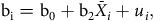
([3.2]) $${\rm{b}_{3i}} = {\rm{ }}{\rm{b}_{30}} + {\rm{ }}{\rm{b}_{31}}{\bar X_i} + {\rm{ }}{r_{3i}}$$

where b₃₀ is the baseline (average) trend in the sample, b₃₁ is the effect of cross-sectional predictor ${\bar X_\rm{i}}$ on the democratic trajectory, and r_3i is a residual component for the random slope. Thus, the latent trend is a function of observed unit-level conditions and unobserved random variance.

By presenting the growth curve estimator as an unconstrained version of Equation 2.1, Equation 3.1 underscores an important point: the country average of time-varying covariate ${\bar X_\rm{i}}$ is a plausible predictor of the random coefficient for T in Equation 3.2, just as it is a plausible predictor of the random intercept in Equation 2.2. While empirical applications of growth curve models tend to emphasize the effect of initial conditions (time-invariant factors) on trajectories, this approach also allows us to capture cumulative effects as conceptualized in the previous section (that is, ḡ*t). For instance, if countries with high average rates of economic growth experience an upward democratic trajectory, the average rate of growth will positively affect the random slope for T in Equation 3.2.

Substituting 3.2, we can restate Equation 3.1 as:

([3.3]) $${Y_{it}} = {\rm{ }}{\rm{b}_0} + {\rm{ }}{\rm{b}_1}({X_{it}}-{\bar X_i}){\rm{ }} + {\rm{ }}{\rm{b}_2}{\bar X_i} + {\rm{ }}\left( {{\rm{b}_{30}} + {\rm{ }}{r_{3i}}} \right){T_{it}} + {\rm{ }}{\rm{b}_{31}}({\bar X_i}^*{T_{it}}){\rm{ }} + {u_i} + {e_{it}}$$

This expression shows that growth curve models account for the latent trend by including interactions between the time counter and cross-sectional variables.Footnote ⁶

Trajectories are not necessarily linear, and we must accommodate this fact to avoid model misspecification (Leite and Stapleton Reference Leite and Stapleton2011). There is no single approach to capture nonlinear trends; latent growth models do so in different ways (Felt et al. Reference Felt, Depaoli and Tiemensma2017, 6–7). To balance sample size requirements and functional flexibility (Whittaker and Khojasteh Reference Whittaker and Khojasteh2017), we employ a cubic polynomial (that is, T, T ², and T ³) and estimate a multiplicative nonlinear latent curve with three random coefficients shaped by the cross-sectional variables (Grimm et al. Reference Grimm, Ram and Hamagami2011, 1363).Footnote ⁷

The theoretical assumptions underpinning growth curve models are closer to intuitive understandings of how many independent variables actually work than the assumptions behind most panel estimators. For example, Paxton et al. (Reference Paxton, Hughes and Painter2010) employ growth curve models to show that democracy did not benefit women’s political representation by the mid-1970s but did influence the growth of women’s political representation over time. Finkel et al. (Reference Finkel, Pérez-Liñán and Seligson2007) show that US democracy assistance incrementally improves levels of democracy above and beyond the otherwise expected country trajectories. Mustillo (Reference Mustillo2009) employs growth curve models to identify a finite mixture of political party trajectories.

Table S1 in the online supplementary materials summarizes the previous discussion by comparing traditional fixed effects models, hybrid effects models, and latent growth curve models. Conventional fixed effects models do not account for cross-sectional variance. The effects of independent variables are not cumulative unless specific measures are created for that purpose (for example, Gerring et al. Reference Gerring, Bond, Barndt and Moreno2005). Other estimators in this family, such as two-way fixed-effects or dynamic panel models, present similar limitations.

Unlike traditional fixed effects models, hybrid estimators seek to explain cross-sectional differences but in a stable way without assuming varying trajectories or cumulative effects. Differences in starting conditions might produce a democratic advantage, but they cannot set countries off on different paths. Similarly, if one country has a higher average rate of economic growth than another, this difference might predict a stable democratic advantage, not one that grows over time – as illustrated by the examples of Argentina and South Korea above.

By contrast, growth curve models assume that initial country characteristics and differences in time-varying predictors with cumulative effects generate a different slope for the latent trajectory. Therefore, the democratic advantage (that is, the gap in the level of democracy) of a country with robust growth compared to one with mediocre growth is likely to expand over time.

The advantages of growth curve models are not technical in a narrow sense. The assumptions underpinning these models fruitfully match our notion of regime trajectories and mirror qualitative work that postulates that many effects can be cumulative, shaping historical trajectories. Growth curve models incorporate these possibilities more than other estimation techniques.

Trajectories in the Third Wave

Our analysis covers all countries that experienced a transition to democracy from 1974 until 2012. We observe democracies on a yearly basis until the regime becomes authoritarian (that is, a breakdown takes place) or until 2017, otherwise. With modest revisions, we build on Lührmann et al.’s (Reference Lührmann, Tannenberg and Lindberg2018) Regimes of the World classification for identifying transitions and breakdowns using V-Dem scores. They distinguished between autocracies and democracies. Following their lead, we code as a transition any shift from either kind of autocracy to either kind of democracy. The inverse change, from democracy to autocracy, we code as a breakdown. Breakdowns mark the end of a democratic regime; after that year, the case drops from our sample. Footnote ⁸

Based on these coding rules, from 1974 to 2017, there were 103 transitions to democracy in 84 independent countries. Regimes enter our dataset in the first full year of democracy, and they exit the year after a breakdown (a new regime begins if they experience another transition to democracy). This yields a total of 1731 country-years in our dataset. We have complete covariate information for 98 democratic regimes and 1595 country-years.

To capture the range of trajectories, we use V-Dem’s Liberal Democracy Index, which is our dependent variable for all country-years in the dataset. V-Dem’s Liberal Democracy scores range from 0 to 1, with 1 representing the highest possible level of democracy (Coppedge et al. Reference Coppedge2020). We rescaled the index to range between 0 and 100.

Of 103 transitions to democracy between 1975 and 2012, a few countries, such as the Baltics, Portugal and Spain, Chile and Uruguay, Slovakia, and South Korea, became robust liberal democracies. In these countries, elections are free and fair, citizens generally enjoy the rights that they are entitled to under democracy, and checks and balances work reasonably well. In other electoral democracies, the effective exercise of rights by citizens is more uneven, opposition rights are often infringed, and mechanisms of accountability are stunted. These regimes have remained democratic but with gaping democratic deficits.

Most countries started the democratic period at mediocre levels of liberal democracy; the average score in the first year for the whole sample is 46 on the 100-point scale. Some countries improved rapidly within a few years (for example, Spain after 1977 and Brazil after 1986), but many declined or remained stagnant. One decade after the transition, only 63 per cent of the regimes had survived, and among them, the average liberal democracy score was 56 points.

The most common outcome, with 45 cases of the 103 transitions in our dataset, was a breakdown of democracy and reversion to authoritarianism by military coup or by executive takeover. Among the 58 regimes that had not broken down as of the end of 2017, the level of liberal democracy varied widely. Although all of these regimes were electoral democracies according to the coding of Lührmann et al. (Reference Lührmann, Tannenberg and Lindberg2018), their average liberal democracy scores ranged between 30 (Lebanon) and 84 (Estonia).

Predictors

To illustrate the advantages of focusing on regime trajectories, our primary predictor of interest is the rate of economic growth. Growth and other covariates might set a latent trajectory by which good performance over time makes it more likely that democracy would deepen, while poor performance would have the reverse effect. We assess growth using the annual per cent change in per capita GDP based on the World Development Indicators (NY.GDP.PCAP.KD.ZG).

Our models control for five variables that potentially confound the effects of economic growth on levels of democracy: per capita income, income inequality, state capacity, the level of democracy among regional neighbours, and the timing of the country’s transition to democracy. (See Table S2 in the supplementary materials for descriptive statistics.) This is a parsimonious set of covariates intended to minimally address confounding. These controls are among the most commonly studied variables in empirical examinations of democracy.

Per Capita Income. A large literature has examined the relationship between the level of development and democracy (Acemoglu et al. Reference Acemoglu, Johnson, Robinson and Yared2008; Boix Reference Boix2011; Boix and Stokes Reference Boix and Stokes2003; Przeworski et al. Reference Przeworski, Alvarez, Cheibub and Limongi2000; Svolik Reference Svolik2015). Because economic growth expands per capita income, it is crucial to disentangle the effects of the two variables. We measure gross domestic product (GDP) per capita in constant 2010 US dollars, using World Development Indicators (NY.GDP.PCAP.KD). We rescale income in thousands of dollars.

Income Inequality. Acemoglu and Robinson (Reference Acemoglu and Robinson2006) and Boix (Reference Boix2003) argued that highly unequal democracies are less likely to survive. We measure income inequality using the Gini index, ranging from 0 to 100, where 0 represents the least inequality and 100 the most inequality. Information for this variable is based on UNU-WIDER (2017) and is extracted from the V-Dem v.5 dataset (e_peginiwi; Coppedge et al. Reference Coppedge2018).

State Capacity. Slater et al. (Reference Slater, Smith and Nair2014) argued that democracy is more likely to break down if state capacity is poor, while O’Donnell (Reference O’Donnell1993) asserted that poor state capacity hinders democratic deepening. We measure state capacity using a composite score of two indices, Hanson and Sigman’s (Reference Hanson and Sigman2013) and Lee and Zhang’s (Reference Lee and Zhang2017). Hanson and Sigman combine three dimensions (extractive, administrative, and coercive) based on a latent variable analysis of twenty-four indicators. Lee and Zhang use census data to estimate the legibility of a state’s population.Footnote ⁹ To minimize missing values, we imputed Hanson and Sigman’s and Lee and Zhang’s indices before conducting a principal components analysis.Footnote ¹⁰ Our composite measure is scaled as a t-index, with a mean of 50 and a standard deviation of 10. Alternative analyses using the two measures separately generated similar results.

Regional Democracy. A region populated with democracies is favourable to the survival of such regimes and perhaps more open to regional trade and growth (Brinks and Coppedge Reference Brinks and Coppedge2006; Coppedge et al. Reference Coppedge and Coppedge2022; Gleditsch and Ward Reference Gleditsch and Ward2006). To assess the regional context, we measure the percentage of countries in each region that are minimally democratic. Following Lührmann et al. (Reference Lührmann, Tannenberg and Lindberg2018), we employ a score equal or greater than 0.5 in the V-Dem polyarchy score as the threshold for minimal democracy.

Year of the Transition. Global trends affect prospects for democracy and economic growth beyond the regional context. To distinguish the regional context from broader global trends, we control for the year when the transition to democracy took place. In contrast to the other predictors, this is not a time-varying covariate. The birth date represents a fixed attribute of each regime.

Estimates

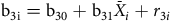
Table 1 below compares results for the three estimators presented in previous sections, using data for our sample of third-wave democracies. Economic growth has no association with levels of liberal democracy in the short run, but it does with levels and trajectories of liberal democracy over the long run.

Table 1. Alternative Panel Models (DV = V-Dem Liberal Democracy score)

Note: Entries are regression coefficients (standard errors). The dependent variable is the Index of Liberal Democracy, rescaled between 0 and 100. The latent trend is modelled with random coefficients. The random variance components are not reported to save space.

* p < 0.05

Model 1.1 reports fixed-effects estimates for five variables: economic growth, per capita GDP, income inequality, state capacity, and regional democracy. The second model (1.2) estimates the same set of ‘within’ effects and also incorporates unit averages to capture ‘between’ effects. This model adds the first year of democracy (the calendar year for t = 0) to the list of cross-sectional predictors. Finally, Model 1.3 expands the specification to capture the latent trend, using a cubic transformation of time and an interaction term for each cross-sectional variable.

Columns 1.1 and 1.2 display almost exactly the same estimates of ‘within’ fixed-effects parameters, with economic growth emerging as an insignificant variable. Only per capita GDP and regional democracy are significant predictors. The results suggest that increases in per capita income or in the percentage of democracies in the region improve levels of liberal democracy in the short run. However, per capita GDP and regional democracy change only gradually over time.

Model 1.2 also captures the effect of cross-sectional variance on the average level of liberal democracy. Countries with faster economic growth and higher per capita income have achieved, on average, stronger liberal democracies, while countries that experienced a transition to democracy later during the third wave have underperformed compared to early democratizers. Those conditions explain average differences in levels of democracy, not change over time. No other cross-sectional variable displays significant effects.

Model 1.3 estimates the latent trend as a function of stable cross-sectional conditions. Due to the complex specification, the interpretation of coefficients in Model 1.3 is not straightforward. In this model, ‘within’ effects capture short-term deviations from the underlying trajectory. Therefore, most coefficients in the top panel lose their statistical significance. Only income inequality appears to undermine expected levels of democracy in the short run, possibly reflecting the social impact of major economic crises.

The coefficients for ‘between’ effects in Model 1.3 are not directly interpretable in terms of size or statistical significance. The effect of cross-sectional predictors on liberal democracy depends on all terms involving ${\bar X_\rm{i}}$ :

([4]) $$\partial {Y_{it}}/\partial {\bar X_i} = {\rm{ }}\left( {{b_2}-{\rm{ }}{b_1}} \right){\rm{ }} + {\rm{ }}{b_{31}}T + {\rm{ }}{b_{32}}{T^2} + {\rm{ }}{b_{33}}{T^3}$$

where b₁, b₂, and b₃₁ correspond to the coefficients in Equation 3.3, and b₃₂ and b₃₃ are (random) coefficients for the interaction of ${\bar X_\rm{i}}$ with the quadratic and cubic transformations of time. Thus, the ‘between’ coefficients in Model 1.3 should not be interpreted in isolation. We focus instead on predicting the association of cross-sectional conditions with democratic trajectories.

Predicting Democratic Trajectories

How much do growth curve models improve our prediction of regime trajectories? A regime’s trajectory is captured by the effect of T (the time elapsed since the transition) on the level of liberal democracy. But, regime trajectories are hard to grasp directly from the coefficients in Model 1.3 for three reasons. First, the effect of T is non-linear (shaped by T, T ², and T ³). Second, the effect of the three terms is captured by a random coefficient – that is, a baseline estimate, illustrated by b₃₀ in Equation 3.2, plus a random component that varies across regimes, r_3i. Third, the baseline effect is moderated by six cross-sectional conditions (that is, b₃₁ ${\bar X_\rm{i}}$ in Equation 3.2), yielding eighteen interaction terms.

To facilitate the interpretation of these results, we provide a graphic representation of predicted democratic trajectories in two steps. As a first step, we compare the predictions of Model 1.2 – a hybrid panel estimator assuming a stationary process – against the regime trajectories predicted by Model 1.3 – a growth curve model relaxing this assumption. We then simulate predicted democratic trajectories under different conditions.

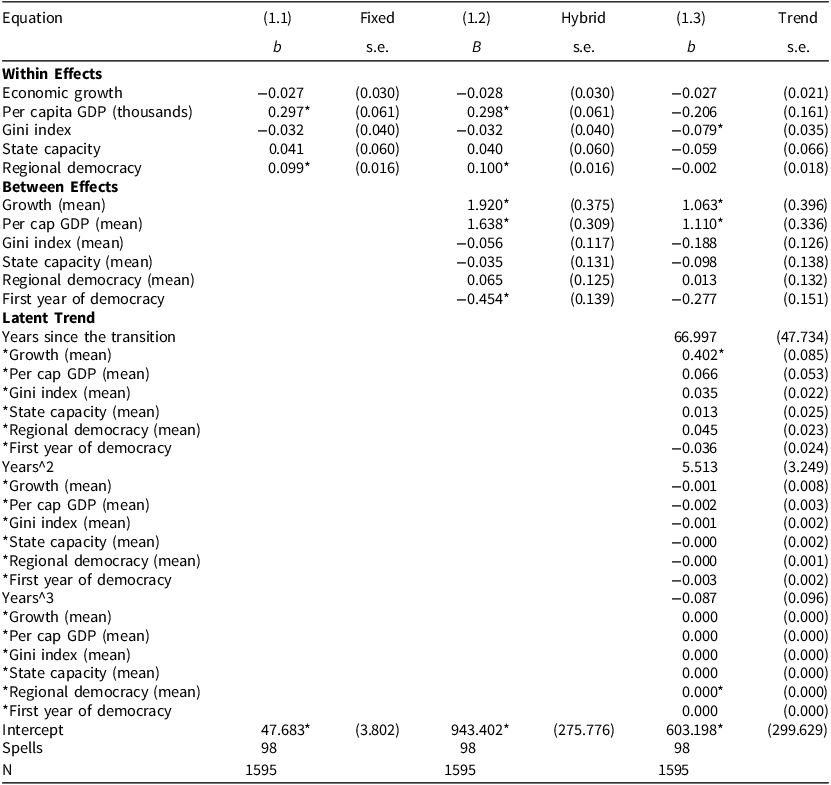
Figure 1 compares the historical trajectories of ten selected countries against the predictions of Models 1.2 (dashed line) and 1.3 (solid line). This contrast underscores the substantive differences between most conventional panel estimators and latent growth curve models. Conventional estimators identify the initial level of democracy – treated as a function of cross-sectional conditions in Model 1.2 – and predict deviations from this level as a function of yearly changes in explanatory factors. This approach anticipates limited change: the dashed line deviates little from initial levels of democracy in most cases. Expected trajectories are flat or have mild monotone trends. Such expectations fail to capture the eventful trajectories of many democratic regimes. Model 1.3 generates better predictions, plotting a distinct trajectory for each regime.Footnote ¹¹ The solid line offers a close representation of actual outcomes, especially in cases that experienced backsliding or breakdown.

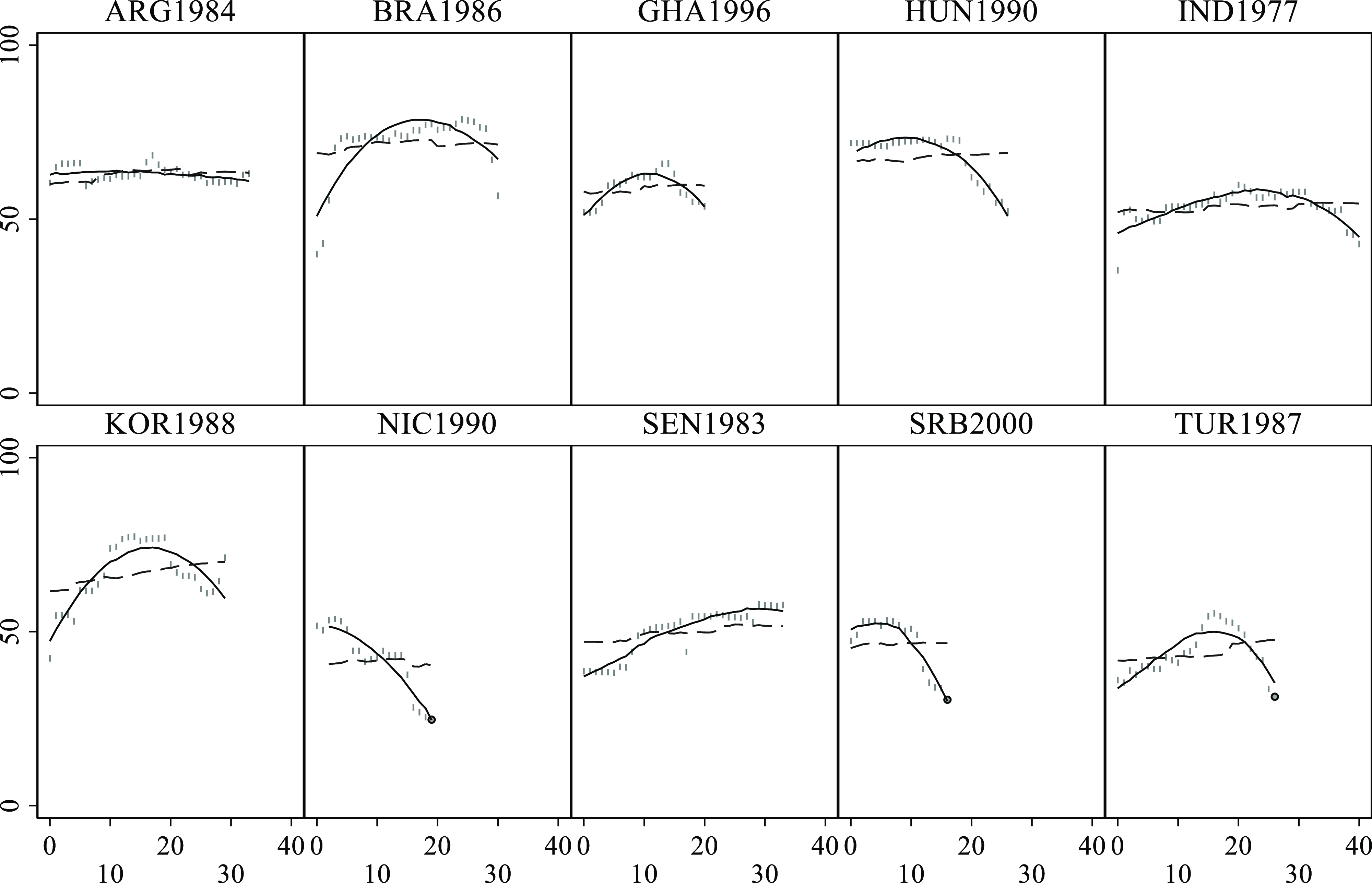
Figure 1. Predicted Democracy Assuming Stationary and Non-Stationary Processes.

Note: The vertical axis displays Liberal Democracy scores. The horizontal axis reflects the years elapsed since the transition. Grey marks are observed in levels of liberal democracy. The dashed line is the prediction of a hybrid model (Model 1.2), assuming a stationary process; the solid line is a prediction of a latent growth curve model (Model 1.3), assuming a non-stationary process. Labels indicate a three-letter country code followed by the first year of democracy. Black dots mark democratic breakdowns.

Besides this visual inspection of selected cases, a comparison of the Root Mean Square Error (RMSE) offers a systematic test of differences in predictive capacity for the whole sample.Footnote ¹² The RMSE is 4.84 for Model 1.1 (fixed effects), 4.85 for Model 1.2 (hybrid), and 2.80 for Model 1.3 (growth curve). There is no meaningful improvement in predictive capacity between Models 1.1 and 1.2, but the growth curve (1.3) reduces the RMSE by 42.3 per cent when compared to either model.Footnote ¹³ Conventional studies have used panel techniques that underestimate the transformation experienced by many regimes. The latent trend approach models change in a more accurate way.

How much can cross-national conditions account for distinct regime trajectories? Our analysis suggests that the inclusion of country averages accounts for almost 50 per cent of the variance in country intercepts and over 50 per cent of the variance in democratic trajectories (Supplementary Table S4). To illustrate the impact of different variables, we employ the coefficients in Model 1.3 to simulate alternative trajectories under selected conditions. Our simulations fix the selected conditions, leaving the remaining predictors at their observed historical levels and averaging expectations across observations. For example, imagine that we want to predict the expected level of liberal democracy for a hypothetical country with an average rate of economic growth of 1 per cent in the second year after the transition to democracy. The simulation fixes the values of growth = 1 and t = 2 for all observations in the sample. Using these values, the observed values for the remaining variables, and the parameters for Model 1.3 (including random effects), it computes the expected level of liberal democracy for all regimes in the sample. As a final step, the procedure takes the average for all regime-years as the predicted score. We then alter the selected conditions, for example, to trace the trajectory of the same case two years later (growth = 1, t = 4) and repeat the procedure.

Figure 2 plots twelve synthetic regime trajectories resulting from 72 simulations. Each panel shows the effect of a particular predictor, comparing the evolution of two hypothetical cases in the decade following a transition to democracy. To distinguish the two hypothetical cases, we set initial conditions at low (straight line) and high (dashed line) levels of the selected predictor, simulating realistic conditions within the observed range of the explanatory variable. The horizontal axis in each panel reflects the time elapsed since the transition, and the vertical axis shows V-Dem liberal democracy scores. The band around each trajectory reflects the 95 per cent confidence interval for the prediction.

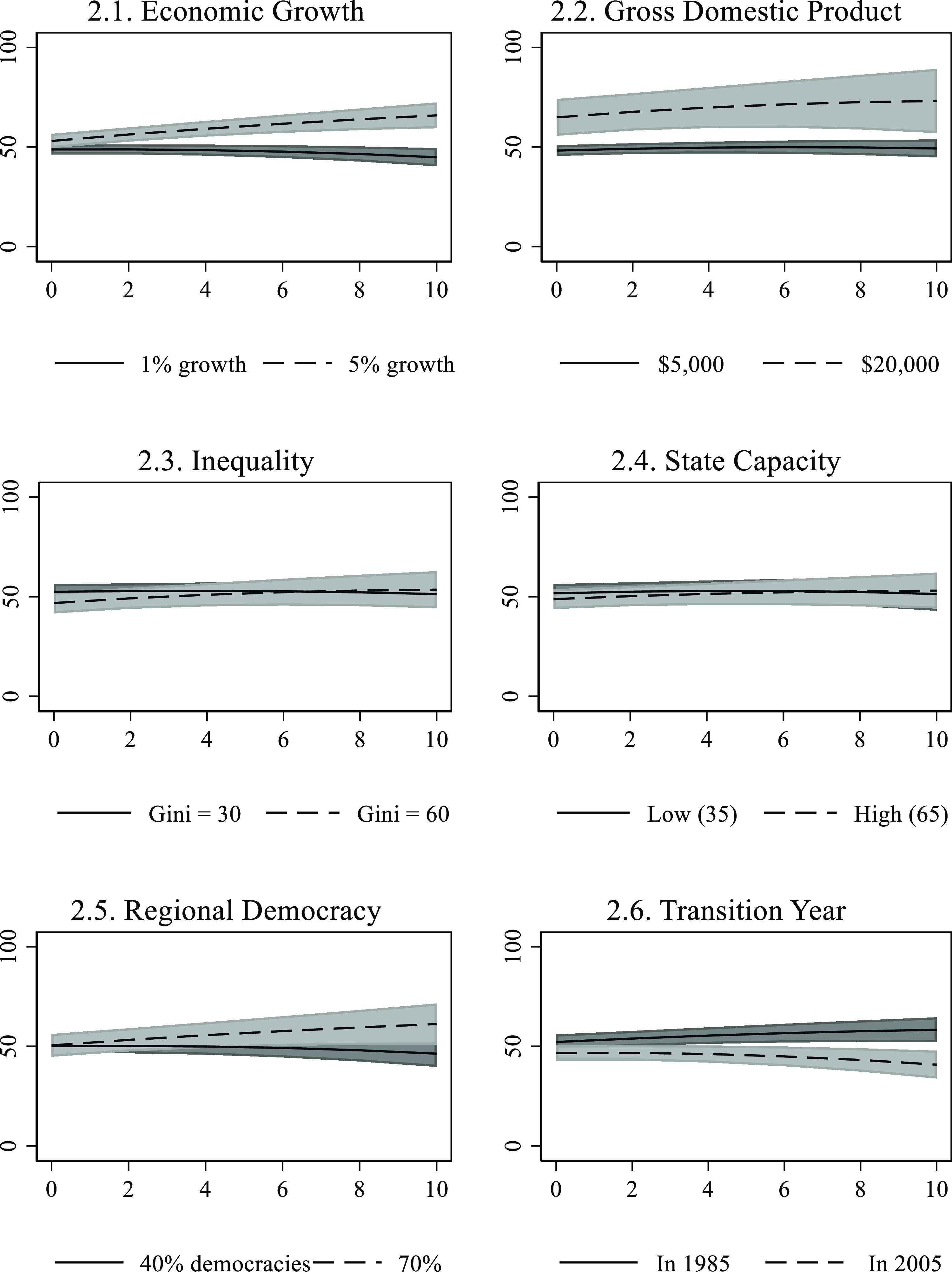
Figure 2. Predicted Trajectories under Selected Conditions.

The six panels in Figure 2 suggest two important conclusions. First and most important for our theoretical argument, some results underscore the advantages of considering how the covariates predict regime trajectories cumulatively over time. For example, economic growth has a distinctive cumulative association with democratic trajectories. Figure 2.1 simulates the effects of the rate of growth, contrasting the consequences of mediocre performance (an average growth rate of 1 per cent per capita per year over a decade) and robust success (a rate of 5 per cent). Initially, the two countries started out with a similar liberal democracy score. Over time, the large difference in growth rates is highly consequential for predicting the level of democracy: in the first case, democracy remains stagnant, while in the second case, liberal democracy trends upwards, improving more than 10 points over the course of a decade. By contrast, in Models 1.1 and 1.2, the coefficients for within-country economic growth are not significant, indicating that short-term growth is not associated with improving liberal democracy scores.

As Figure 2.1 shows, the association between higher growth and more robust democracy manifests only over time. This underscores the key point of this paper. Robust economic growth over time is associated with a positive long-term trajectory for democracy, and sluggish growth over time is associated with democratic stagnation. Fixed effects and hybrid effects models do not capture these cumulative effects. We cannot rule out the possibility of reverse causation between growth and democracy, but an instrumental variable analysis suggests that the pattern in Figure 2.1 remains even after we account for this possibility (see Table S6 and Figure S1 in the supplementary materials).

Second, most simulations display a flat trajectory for the average regime in the third wave of democratization. Despite the considerable variation in individual trajectories observed in Figure 1, the typical trend in most simulations shows little change. Stagnation, more than democratic progress or backsliding, is the most likely outcome predicted by our model.

However, some covariates predict distinct trajectories. Figure 2.2 on the right compares the trajectory of two hypothetical regimes, one with an average per capita GDP of $5,000 and another with a per capita GDP of $20,000. The wealthier country starts out with a more robust liberal democracy. Its democratic advantage expands over time as its level of democracy improves, while the poorer countries stagnate. Intuitively, it makes sense that the structural advantages of higher development facilitate a higher level of democracy from the outset, whereas the democratic advantages of better economic performance emerge only over time. Together, these findings suggest that economic conditions have profound long-term implications for regime trajectories.

The two panels in the middle row of Figure 2 simulate the effects of two variables believed to affect democratization: income inequality and state capacity. Both are likely confounders for the effects of economic growth. Against expectations, neither variable has much association with regime trajectories. The predicted trends are virtually indistinguishable over time.

The bottom panels underscore the relevance of international factors. On the left, the simulation captures the distinction between a hypothetical country in an authoritarian neighbourhood (only 40 per cent of the countries in the region have scores greater than 0.5 in V-Dem’s Electoral Democracy Index) and one in a ‘good neighbourhood’ (70 per cent). The two countries start at around 50 points on the Liberal Democracy scale but separate over time. While the first case declines slightly, the second case improves by about 10 points over the course of a decade, converging towards the norm for its region.

The last panel suggests that global conditions for new democracies have worsened over time, consistent with recent writings on democratic erosions (Lührmann and Lindberg Reference Lührmann and Lindberg2019). The typical democracy born in 1985 started from a slightly better position (52 versus 47 points) and experienced a better trajectory than the one born in 2005. In the simulation, the older regime experienced an improvement of about 6 points over time, while the newer regime experienced a decline of similar magnitude. Thus, by the end of their first decade, the two regimes were in significantly different situations.

Summarizing the substantive implications of Table 1, countries with higher growth rates, those located in a more democratic neighbourhood, and those that experienced an earlier transition did not achieve higher levels of democracy compared to other countries immediately after the transition, but they did so over time. Wealthier countries began at a higher level of democracy, and this democratic advantage grew over time. The evidence thus underscores the important role of cumulative effects that defy traditional assumptions about stationarity.