


Introduction
In the early phase of product development, design engineers are often required to determine the means necessary to achieve the intended main functionality. Multiple alternatives to such means give rise to discrete design spaces, where combinations of ideas form the basis for new concepts. Depending on the nature of the development project, such as if it is a new or derivative development project, the considered means can either be new, existing, or a combination of the two. In such design scenarios, it may not be possible to identify promising designs using traditional optimization processes because (i) it is too early in the design process to conduct simulations or physical tests or (ii) novel configurations of previously developed subsystems may render existing analytical models nonrepresentative. For these reasons, expert opinion is required to identify promising configurations. However, exploring vast discrete design spaces through expert opinion alone makes it difficult to ensure that all promising configurations have been considered.
To explore discrete design spaces, designers have the option to use morphological matrices (MMs) (Zwicky, Reference Zwicky, Zwicky and Wilson1967). MMs list all functions that are necessary to fulfill the main function, together with all considered means that can achieve each function. By combining means, one for each function in the MM, a potential solution candidate is generated. However, one of the major issues with this approach is that the number of possible combinations is often out of bounds from what a team of engineers can realistically consider for further development, due to time constraints (Motte and Bjärnemo, Reference Motte and Bjärnemo2013). To exemplify this, consider the study conducted by Almefelt (Reference Almefelt2005), which resulted in an MM with eight functions, and up to 22 alternative means for each function. That results in a theoretical maximum of about 54.9 billion possible combinations. Such a vast number of combinations cannot possibly be considered manually. However, the exact threshold for what is considered a too-large design space will naturally vary depending on the size and experience of the engineering team working on the problem. Furthermore, the traditional MM is used to support concept generation, but not evaluation. Thus, it assists in the identification of concepts, but not in determining their fitness. In other words, the traditional method contains no mechanism to assist in identifying the most promising solutions.
At the same time, commitment to means at this stage of development may either enable or inhibit future changes to the system. As Buede (Reference Buede2016) put it, “The mark of a long-lived system is one that has been upgraded successfully many times.” Fricke and Schulz (Reference Fricke and Schulz2005) refer to upgradable systems as being flexible. Examples of design scenarios where designing for flexibility is critical include the following:
-
1. The system needs to be configurable such that it can handle varying customer requirements.
-
2. The system needs to be upgradable such that additional modules or features can be retrofitted or swapped out. This can, for instance, enable the lifetime of the product to be extended (Khan et al., Reference Khan, Mittal, West and Wuest2018).
-
3. The system that is being designed needs to account for future technologies. Accommodating such future technologies can reduce the need for straying from the original design in future product iterations, thus enabling the reuse of existing assets (Martinsson Bonde et al., Reference Martinsson Bonde, Kokkolaras, Andersson, Panarotto and Isaksson2023).
-
4. Any combination of previously listed scenarios.
Situation 1 includes scenarios such as having the customer be able to select different design configurations and also scenarios where it is possible for the user to procure modules after purchasing the original product. Situation 3, on the other hand, can be of interest when designing within a product family (Simpson et al., Reference Simpson, Maier and Mistree2001). One of the main purposes of product families is to reuse assets, both tangible and intangible, between product iterations. Therefore, designing with the compatibility of future technologies in mind ensures that a greater overlap exists between the existing design and future designs, thus increasing the possibilities of asset reuse. In either scenario, considering flexibility already during concept design has the potential to assist designers in understanding the future of the system, and its subcomponents, enabling them to make better-informed decisions.
The aim of the research presented in this paper is to explore ideas for how MMs can be used to support design, with a focus on (i) efficient exploration of large discrete design spaces and (ii) accounting for design flexibility, while also accounting for other design objectives such as performance and cost. We focus on the following research question: How can vast discrete design spaces be explored with respect to design objectives and flexibility? By vast discrete design spaces, we mean spaces that are difficult for engineers to explore without support due to the combinatorial explosion often created by MMs.
Theoretical background
Design space exploration in the early stages of design has been covered thoroughly in academic literature. Key examples of this include Hubka (Reference Hubka1982), Pahl et al. (Reference Pahl, Beitz, Feldhusen and Harriman2007), and Ulrich et al. (Reference Ulrich, Eppinger and Yang2020). A design generation method found in all three of these well-recognized works is the MM. The MM is typically preceded by a functional decomposition of the problem. First, a main function is defined that, when performed, solves the design problem. This main function is then decomposed into smaller functions that, when combined, achieve the main function. The idea of the MM is to collect means that can achieve functions identified through decomposition. By combining one means for each function, a solution candidate can be conceived.
A prominent issue with MMs is the vast number of potential solutions that can spring from only a few functions and means. This combinatorial explosion often makes it challenging to consider all possible combinations in the MM. Thus, high-performing combinations can remain undiscovered. In the “Exploring large discrete design spaces” section, different ideas for how to deal with this problem are explored. Additionally, since this research aims to contribute a method for including flexibility when using MMs, the “Evaluating and trading for design flexibility” section is dedicated to contemporary means of accounting for flexibility in design space exploration.
Exploring large discrete design spaces
Design space exploration is the act of representing and evaluating design variants (Woodbury and Burrow, Reference Woodbury and Burrow2006). In contrast to design spaces conceived through continuous variation of design variables, such as dimensional values, the design space spanned by an MM is discrete in nature, as it is a set of combinations that are being considered (Zwicky, Reference Zwicky, Zwicky and Wilson1967). Discrete design spaces are encountered in the early phases of design when different means are considered for achieving the various functions of the system. This includes new product development scenarios in which information concerning the alternative means is scarce. It also includes scenarios in which more is known about the alternatives, such as when configuring design variants within a product family (Siddique and Rosen, Reference Siddique and Rosen2001).
To make discrete design space exploration more manageable, different approaches have been proposed. Motte and Bjärnemo (Reference Motte and Bjärnemo2013) divide these approaches into two categories: automatic or semi-automatic exploration and reduction through heuristics. Motte and Bjärnemo (Reference Motte and Bjärnemo2013) further outline multiple approaches within each category, some of which are discussed here alongside additional approaches.
Ulrich et al. (Reference Ulrich, Eppinger and Yang2020) state that means that are not feasible should be excluded from the MM. Yet clarity regarding the feasibility of design alternatives is not always evident in the early phases of the design process. It can, however, be possible to determine if a specific combination is infeasible due to incompatibilities among means. For instance, different means may rely on different energy sources or material flows. Pahl et al. (Reference Pahl, Beitz, Feldhusen and Harriman2007) suggest that such incompatible pairings of means are identified so that they can be avoided. These methods do not require the use of software or computational resources, but their impact on the number of possible combinations is small.
Experiments conducted by Smith et al. (Reference Smith, Richardson, Summers and Mocko2012), together with engineering students, suggest that large MMs, especially those with many functions relative to the number of means, can result in lower-quality concepts. Consequently, for manual exploration of MMs, it can be beneficial to restrict the decomposition of functions and keep them at a high level.
Instead of reducing the size of the design space by excluding means, or combinations of means, Almefelt (Reference Almefelt2005) suggests an alternative approach. The functions are sorted with respect to complexity in terms of how much they interact with other functions within the system. Then, focus is put on identifying high-performing interactions between means within the functions that have the highest complexity. Consequently, combinations with high levels of positive interactions are found more rapidly, while other combinations can be discarded, thus delimiting the design space.
The aforementioned approaches are based on heuristics, and manual navigation through the discrete design space. An alternative approach is to let a computer perform the navigation or to combine manual navigation with computational means, which Motte and Bjärnemo (Reference Motte and Bjärnemo2013) refer to as automatic or semi-automatic exploration. However, to enable a computer to make decisions using a morphological approach, additional information is needed. This can, for instance, be provided by attaching mathematical models to the means or by quantifying the desired attributes of the means.
Bryant et al. (Reference Bryant, Bohm, Stone and McAdams2007) developed a web-based tool for generating concepts. The user is asked to input which functions the system needs to achieve. Using a repository of existing concepts, the tool identifies alternative means for the functions. The tool can then be used to generate concepts, which is done by evaluating which combinations of means are feasible based on previous concepts. The tool can also be used interactively to, rather than generate concepts, assist the user in selecting feasible combinations.
Ölvander et al. (Reference Ölvander, Lundén and Gavel2009) and Tiwari et al. (Reference Tiwari, Teegavarapu, Summers and Fadel2009) enriched the means in the MM with mathematical models to describe properties such as weight and cost and used optimization to identify promising solutions. The approach demonstrated by Ölvander et al. (Reference Ölvander, Lundén and Gavel2009) is based on the Tabu search, while Tiwari et al. (Reference Tiwari, Teegavarapu, Summers and Fadel2009) instead used a genetic algorithm. Notably, these methods also consider incompatible combinations, as the designer can formulate incompatibilities in the form of optimization constraints.
Ma et al. (Reference Ma, Chu, Xue and Chen2017) used fuzzy programming to represent customer preferences, determining the values using fuzzy pairwise comparison. In addition, the authors introduced an element of reliability such that the MM could be optimized with respect to two separate objectives: customer satisfaction and product reliability.
Using optimization algorithms in this way entails that enough detailed information about each means is obtainable such that the mathematical models can be populated. However, the resolution of these mathematical models is typically limited by the scarcity of information in the early phases of design. Consequently, the models may need to be populated through the application of qualitative information, such as expert opinions or experience from previous projects.
Some morphological approaches emphasize the application of expert opinion. One such approach is the advanced morphological approach (AMA), which was introduced by Bardenhagen and Rakov (Reference Bardenhagen and Rakov2019). AMA aims to reduce the dimensionality of the MM and then uses a mixture of random solution generation and expert selection to identify high-performing solution variants. Further work was recently conducted by Todorov et al. (Reference Todorov, Rakov and Bardenhagen2022) to refine AMA by incorporating fuzzy sets as a means to codify expert knowledge, enriching its possibility to identify promising solutions based on certain criteria. Another approach, which used enhanced function-means (F-M) trees for design space exploration, was proposed by Müller et al. (Reference Müller, Isaksson, Landahl, Raja, Panarotto, Levandowski and Raudberget2019). This approach combined all possible alternative means in an F-M tree into concepts. However, the means of the tree were enhanced with additional information such as constraints and design variables. This information allowed for concepts to be screened automatically, but also partially based on expert opinion.
Evaluating and trading for design flexibility
Design freedom is a concept commonly used to refer to the degree to which a design can be adjusted while still meeting requirements (Simpson et al., Reference Simpson, Rosen, Allen and Mistree1998). The well-known design paradox stipulates that, when the most is known about the design, designers have the least amount of freedom to act on that knowledge (Ullman, Reference Ullman2002). In other words, as the design space becomes increasingly constrained over time, the design freedom is reduced. Design freedom can also be constrained from the very start of a product development project, for instance, due to the constraints of the product platform upon which the product is being built. An example of this in the automotive industry is the stylistic elements associated with brands, which can significantly constrain the design space from the very start (Burnap et al., Reference Burnap, Hartley, Pan, Gonzalez and Papalambros2016).
Retaining design freedom for as long as possible is generally favorable, as demonstrated by practices such as set-based concurrent engineering (Sobek et al., Reference Sobek, Ward and Liker1999). Flexibility, described by Fricke and Schulz (Reference Fricke and Schulz2005) as a system’s ability to be easily changed, is a means of preserving a degree of design freedom throughout a system’s life cycle. A flexible system allows for life-cycle upgrades, such as retrofitting new components or modules, and extends to upgrading a product platform within a product family (Simpson et al., Reference Simpson, Maier and Mistree2001). Thus, a flexible platform can accommodate emerging requirements and novel technologies through necessary external changes.
Making changes to a subsystem is likely to affect other components of the system. One way to quantify this is through change propagation (Clarkson et al., Reference Clarkson, Caroline and Claudia2004), which measures how other subsystems are affected by a change to one system. This highlights the need to design for flexibility, as high flexibility entails reduced impact on the rest of the system, in the event of a change. However, for a system to be successful, it must also be performant. Therefore, there is a need to balance flexibility with other system properties, such as weight and cost. To enable trading flexibility against other system properties such as performance, the flexibility of a design first needs to be quantified. To that end, a range of studies have proposed metrics for measuring flexibility in engineering design. For instance, Hölttä and Otto (Reference Hölttä and Otto2005) introduced a procedure for designing products with a flexible architecture, using a redesign effort complexity metric to minimize redesign effort. They emphasize the need for designing modules and module interfaces such that changes to a module require minimal rework. Cormier et al. (Reference Cormier, Olewnik and Lewis2008) focused on design flexibility for mass customization, proposing metrics to evaluate the overall flexibility of a system. This emphasizes the importance of systems to enable the fulfillment of many different needs, while at the same time being efficient in the utilization of common resources. Recently, Alonso Fernández et al. (Reference Alonso Fernández, Panarotto and Isaksson2024) showed how to accommodate future technologies by demonstrating a flexibility trade-off method with a focus on reserving geometric space for future upgrades and managing the risk of failure propagation. Field effects were used to evaluate the ability of subsystems to function within a geometric region, indicating how the system could handle the integration of new technologies. There exists a large set of alternative methods for quantifying flexibility, which depends heavily on context and application. For a more thorough review of alternatives, Machchhar et al. (Reference Machchhar, Bertoni, Wall and Larsson2024) recently conducted a review on the topic.
Design margins play a crucial role in managing flexibility within product platforms. These margins, which represent the buffer or excess capacity built into a design, allow for adaptability and future upgrades without significant redesign (Eckert et al., Reference Eckert, Isaksson, Lebjioui, Earl and Edlund2020). In the context of product platforms, design margins help absorb the impact of changes and new requirements, facilitating smoother integration of new technologies and reducing the need for extensive rework. By incorporating adequate design margins, systems can maintain performance and accommodate unforeseen demands, thus enhancing overall robustness and longevity. However, managing these margins effectively is essential to avoid overdesign and underdesign, which can respectively lead to unnecessary costs or potential system failures. A recent review by Brahma et al. (Reference Brahma, Ferguson, Eckert and Isaksson2024a) provides a comprehensive analysis of margins in engineering design, outlining their definitions, applications, and methods for effective management of margins. This review highlights the divergent and fragmented understanding of margins across different domains and proposes a unified framework to better manage margins systematically. The authors differentiate between deliberately added margins and those that arise inadvertently, emphasizing the importance of strategic margin allocation to mitigate uncertainties and ensure robust, flexible design. This systematic approach is crucial for enhancing the upgradability and longevity of product platforms, as it helps in accommodating future changes and minimizing redesign efforts.
The large number of papers on the topic of flexibility suggests that there is a need to better understand how systems can be designed to be upgradable. This need seems to be driven by the necessity to minimize design rework, extend the life of systems such as product platforms, and cater to the needs of multiple market segments while maintaining resource efficiency through commonality. One of the main challenges is to ensure that the existing system can handle the change without negatively affecting other parts of the system. Thus, evaluating flexibility already in the early stages of design is critical. The method presented in the “Multi-objective technology assortment combinatorics” section can mitigate these issues by providing an early indication of flexibility and assisting in the selection of flexible concepts.
Multi-objective technology assortment combinatorics
Multi-objective technology assortment combinatorics (MOTAC) is an approach to flexible product design. It assumes a system that achieves a set of functions and that there are alternative ways of achieving those functions.
The first step of the approach is to perform a functional decomposition of the system in the form of an F-M tree. Alternative means are provided to the functions of the system within the confounds of an MM.
The second step is to identify pairings of means that are unfeasible. In addition to assisting the pathfinding algorithm in identifying feasible combinations, this step also provides the basis for the flexibility evaluation, as a means that cannot easily be combined with other design solutions is less flexible.
The third step involves defining objectives and quantifying each means in the matrix based on those objectives. A penalty function also needs to be defined. The penalty function is a mathematical function that determines how much a means is penalized in the automated selection process. How much a means is penalized depends on how performant it is with respect to the previously defined objectives.
In the fourth step, a selection process is conducted using a pathfinding algorithm, which strives to find the path through the MM with the least amount of penalties. In doing so, it identifies solution candidates, which manifest as combinations of means in the MM. A visual representation of the method can be seen in Figure 1.
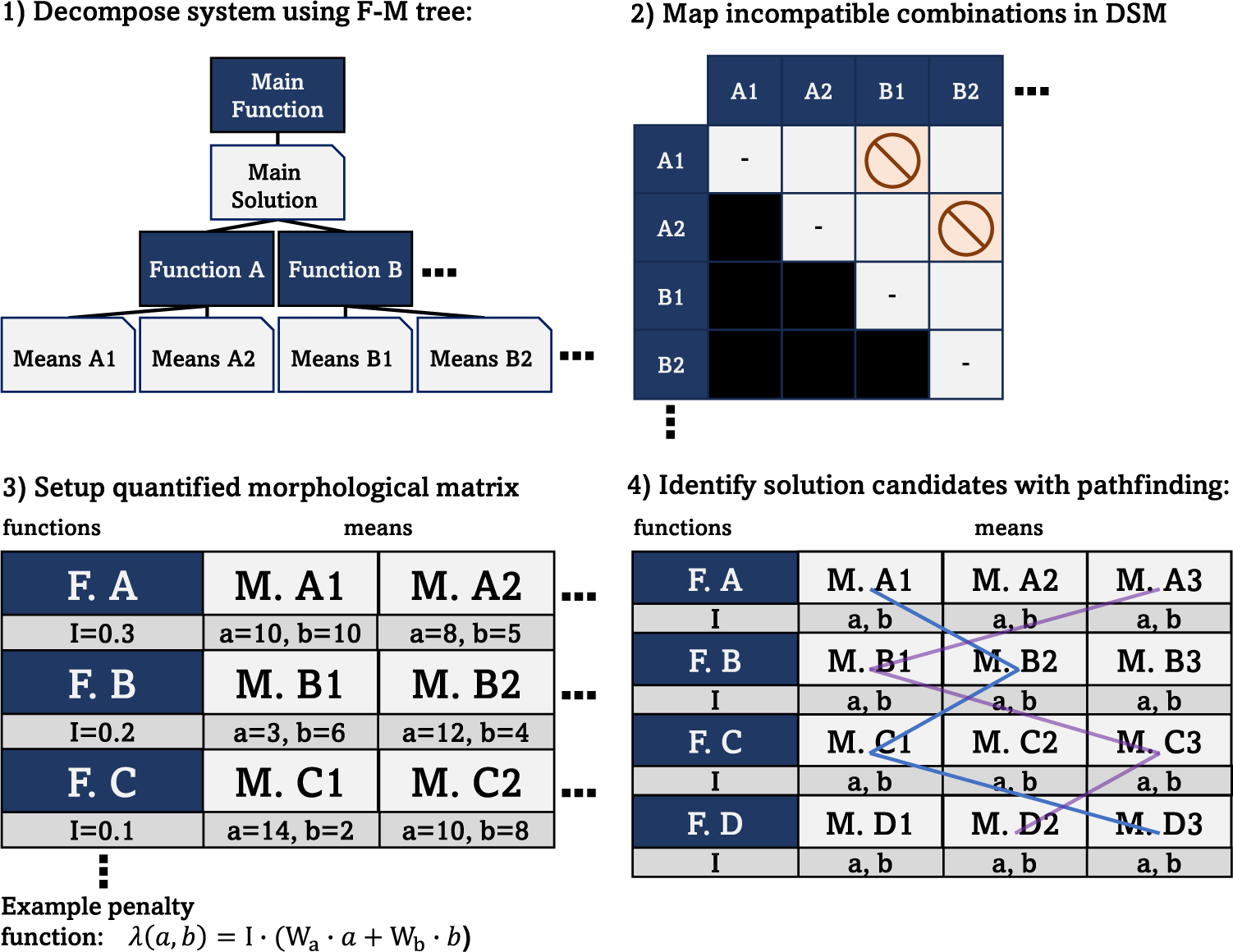
Figure 1. Visualization of the MOTAC approach.
These four steps grant an overview of MOTAC. The remainder of this section describes MOTAC in detail, going through each step.
Functional decomposition and identification of incompatibilities
Initially, the system functionality is modeled using an F-M tree. When designing for a product family, the functions performed by the system often overlap between product iterations. Therefore, in such a scenario, it is possible to either (1) functionally decompose an existing product from within the product family or (2) reuse the F-M tree model from a previous product. Additional functions can be added, if necessary.
Once the structure of the F-M tree is completed, additional means can be added. Having more than one means for one individual function entails that there are options. Once all options are in place, incompatible means are identified and marked. This can, for instance, be done by drawing lines between the incompatible means in the F-M tree or using a design structure matrix (DSM).
The system functionality and its alternative means, as contained in the F-M tree, are then mapped onto an MM. However, a typical MM does not take into account higher-level functions. Therefore, only the lowest level of functions in the F-M tree are used in the MM. Consequently, for the method to work as intended, alternative means cannot exist on higher levels in the F-M tree, as that would also entail alternative functions, which are not compatible with the conventional MM method without creating multiple MMs.
Setting up the quantifiable morphological matrix
The low-level functions and their alternative means are used to compose an MM. At this stage, it is also possible to add additional alternative means to the matrix. Once all the functions and means are in place, the design objectives need to be defined. The design objectives are to be used to identify promising combinations of means, referred to here as solution candidates. Thus, the design objectives need to be key attributes that are important to the success of the potential product. Such objectives may, for instance, involve weight, cost, performance, and manufacturability. As is further discussed in the “Accounting for flexibility” section, the design objectives may also concern flexibility.
Next, the attributes need to be represented numerically for each means in the MM. How this is conducted can vary significantly depending on how much is known about the system and each individual means. It is indeed possible to attribute a means with its exact weight and cost, although it is often the case that this information is unknown. Preferably, all means should have the same attribute resolution. Commonly in the early design phase, information is scarce. Even if the individual means are known from previous projects, it is often uncertain how they will behave when combined in novel ways (Stenholm et al., Reference Stenholm, Corin Stig, Ivansen and Bergsjö2019). Thus, a fitting method of determining attribute values for each means in the MM is through the application of pairwise comparison, where the means of each function are compared with each other. Similarly, pairwise comparison can be used to determine the importance of the design objectives. This enables the formulation of a penalty function $ \lambda $
that follows the pattern of a weighted linear combination, as seen in Equation (1)), where there are
$ \lambda $
that follows the pattern of a weighted linear combination, as seen in Equation (1)), where there are $ n $
design objectives.
$ n $
design objectives. $ {x}_{a,b} $
represents the performance of means
$ {x}_{a,b} $
represents the performance of means $ b $
with respect to design objective
$ b $
with respect to design objective $ a $
. The objective performance of each means is multiplied with their respective objective coefficient, determined through pairwise comparison, the sum of which is multiplied by the importance of the function
$ a $
. The objective performance of each means is multiplied with their respective objective coefficient, determined through pairwise comparison, the sum of which is multiplied by the importance of the function $ {I}_{\mathrm{F}i} $
each multiplied by an objective coefficient
$ {I}_{\mathrm{F}i} $
each multiplied by an objective coefficient $ {\mathrm{W}}_a $
. This calculation is performed and summed over each means (
$ {\mathrm{W}}_a $
. This calculation is performed and summed over each means ( $ k $
) to determine the penalty value for a combination of means. It should be noted that, since this process contains plenty of uncertainty, it is recommended to perform a sensitivity analysis, an aspect that is further discussed in the “Possible improvements” section:
$ k $
) to determine the penalty value for a combination of means. It should be noted that, since this process contains plenty of uncertainty, it is recommended to perform a sensitivity analysis, an aspect that is further discussed in the “Possible improvements” section:
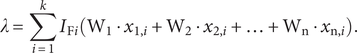 $$ \lambda =\sum \limits_{i=1}^k{I}_{\mathrm{F}i}\left({\mathrm{W}}_1\cdot {x}_{1,i}+{\mathrm{W}}_2\cdot {x}_{2,i}+\dots +{\mathrm{W}}_{\mathrm{n}}\cdot {x}_{\mathrm{n},i}\right). $$
Identifying promising combinations with pathfinding
The MM can be considered as a network of nodes, within which there is only one possible direction to travel. By modeling the MM as a network of nodes, a pathfinder algorithm, such as Dijkstra’s algorithm (Dijkstra, Reference Dijkstra1959; Skiena, Reference Skiena1998), can be used to navigate it. The pathfinder needs to traverse from one function to the next, without ever visiting the same function twice. A node in this network is a representation of a means. If the performance of a means with respect to the design objectives can be rephrased as a penalty function, then the nodes in the path of the least aggregated penalty will compose the highest performing solution candidate. In addition, the objective coefficients in the penalty function can be rebalanced depending on the importance of different criteria.
It also becomes possible, through slight modifications to Dijkstra’s algorithm, to consider incompatibilities. Each node is instantiated with a set of incompatibilities that matches the ones listed in the DSM. An example of how such a node can be implemented is demonstrated in Pseudocode 1.
Pseudocode 1. Node definition for use in pathfinding in morphological matrices.
class Node:
m: Means # The means this node represents
previous: Node # Previously traversed Node
incomp_set: set = m.incomp_set.union(previous.incomp_set)
penalty_aggregate: float = m.penalty + previous.penalty_aggregate
Before the algorithm traverses from one node to another, it is first confirmed that the next node does not belong to the set of incompatible means. If it is not part of the incompatible set, then the next node is visited. At the same time, the incompatibilities of the previously visited node are inherited by the current node. Thus, to adjust Dijkstra’s algorithm, the nodes need to inherit the incompatibilities of the means it represents and all previously visited means in the path. Then, before queuing the means in the next function, they are checked against the set of incompatible means to assert that the queued nodes are compatible with the already visited nodes. An example of how this can be implemented is demonstrated in Pseudocode 2, where a priority queue (Skiena, Reference Skiena1998) has been used to sort the nodes based on penalty such that the node with the lowest penalty is always returned from the queue.
Pseudocode 2. Pathfinding algorithm for morphological matrices with incompatible means.
def generate_solution():
# Instantiate Priority Queue sorted by aggregated node penalty
pq = PriorityQueue()
# Add one node for each of the means in the first function to the queue
for m in first_function:
pq.insert(Node(m=m, previous=None))
while pq.isEmpty() is False:
current_node = pq.find_minimum()
next_f = get_next_function()
if next_f is None:
return create_solution(current_node)
# Only queue compatible means from next function
for m in next_f:
if m in current_node.incomp_set:
continue
pq.insert(Node(m=m, previous=current_node))
The key differences from the traditional pathfinding algorithm are (i) nodes in the network are only linked in one direction to nodes of the next function, (ii) nodes keep track of incompatibilities gained through the path, and (iii) a node that is incompatible with any previous node cannot be visited.
It should be noted that, while the pathfinding algorithm will identify the path with the least aggregated penalty, it is still advisable to use this method to generate multiple solutions and not just one. This is especially true if the attributes have low resolution, which entails a high degree of uncertainty. Screening a larger set of solutions will thus increase the chances of identifying high-performing solution candidates for further development. Modifying the pathfinding algorithm to return $ N $
number of solutions is a trivial adjustment.
$ N $
number of solutions is a trivial adjustment.
Accounting for flexibility
As covered in the “Introduction” section, there are multiple scenarios where designers can benefit from taking flexibility into account when exploring the design space. To achieve this using MOTAC, flexibility also needs to be included in the penalty function, thus penalizing combinations that are less flexible. To achieve this, flexibility first needs to be quantified. We propose calculating the impact of committing to a means on the available design space. In other words, how much of the design space becomes unavailable as a consequence of committing to a specific means? This can be quantified as a ratio between the constrained and unconstrained design spaces. The design space becomes constrained by committing to means in the MM that are incompatible with other means. Consequently, if a means is compatible with all other means in the MM, then there is no negative impact on the available design space due to that means, and thus the flexibility is high. On the other hand, if a choice of means prevents the selection of other means, then that choice results in a lower flexibility as it constrains the design space. The flexibility can thus be formulated as in Equation (2), where $ {f}_i $
is the impact on flexibility by choosing means
$ {f}_i $
is the impact on flexibility by choosing means $ i $
,
$ i $
, $ {N}_{\mathrm{constrained}} $
is the number of possible design candidates where
$ {N}_{\mathrm{constrained}} $
is the number of possible design candidates where $ i $
is included, and
$ i $
is included, and $ {N}_{\mathrm{unconstrained}} $
is the number of available design candidates where
$ {N}_{\mathrm{unconstrained}} $
is the number of available design candidates where $ i $
is included if there were no incompatibilities. As such, this is a metric of combinatorial flexibility, given the choice of a particular means, where a lower value entails a higher flexibility. A visualization of how the metric works can be seen in Figure 2.
$ i $
is included if there were no incompatibilities. As such, this is a metric of combinatorial flexibility, given the choice of a particular means, where a lower value entails a higher flexibility. A visualization of how the metric works can be seen in Figure 2.
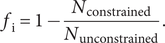 $$ {f}_{\mathrm{i}}=1-\frac{N_{\mathrm{constrained}}}{N_{\mathrm{unconstrained}}}. $$
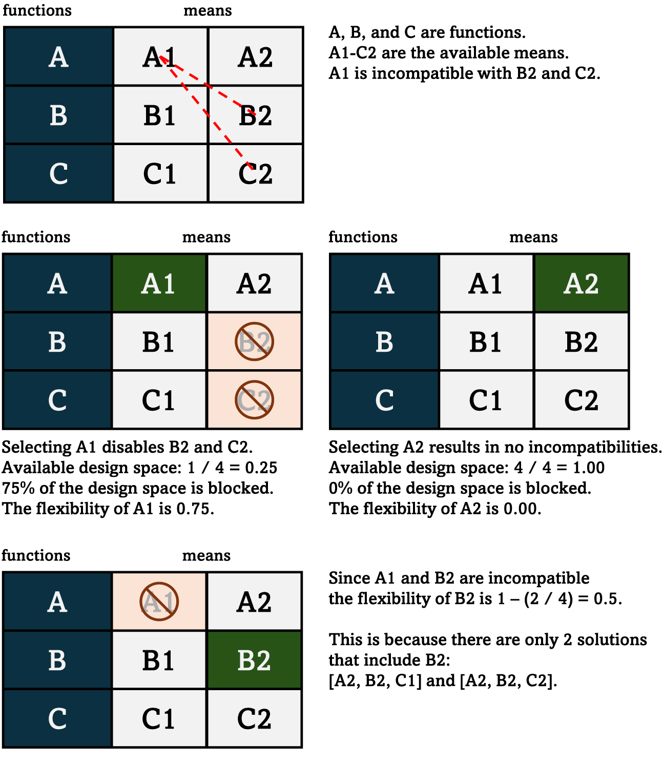
Figure 2. Visualization of the proposed metric for combinatorial flexibility and its application in morphological matrices.
A slight complication occurs in scenarios where multiple incompatibilities overlap. Whether or not the same incompatibility should be counted twice is a matter of discussion. Consider Figure 2, which depicts an MM that has three functions: A, B, and C. Each of the three functions has two alternative means: A1 and A2, B1 and B2, and C1 and C2. Both B2 and C2 are incompatible with A1. If the combination A2–B2–C2 is evaluated, then the incompatibility with A1 occurs twice: once with B2 and once with C2. It can be argued that if B2 has already been selected, then it makes no difference if C2 has the same incompatibility, and thus it should have no impact on the flexibility. On the other hand, counting each occurrence of an incompatibility can potentially provide an indication of how entrenched it is. Another point to consider is that counting incompatibilities only once is more computationally expensive since the algorithm needs to keep track of which incompatibilities have already been encountered. Conversely, if there is no need to keep track of existing incompatibilities, then the flexibility of each means can be calculated before the pathfinding algorithm begins since it is independent of previous selections. Nevertheless, the impact on computational expenses is minor and unlikely to be an issue. A final point on this matter: counting the same incompatible means more than once can result in scenarios where a system with only one incompatible means is deemed less flexible than a system with two or more incompatible means. For this reason, throughout the rest of the presented research, the first alternative was used. In other words, incompatible means were counted only once.
Example: Steer-by-wire system
To test and demonstrate usage of the MOTAC approach, the method and algorithms proposed in the “Multi-objective technology assortment combinatorics” section were implemented as new features in previously developed software used to create F-M trees and MMs (Martinsson Bonde et al., Reference Martinsson Bonde, Mallalieu, Panarotto, Isaksson, Almefelt and Malmqvist2022; Martinsson Bonde et al., Reference Martinsson Bonde, Breimann, Malmqvist, Kirchner and Isaksson2024). This ensured that the method can indeed be integrated and used with a computer and that the algorithms are computationally inexpensive.
Using these software, a steer-by-wire (SbW) design scenario was studied. SbW is being increasingly considered for commercial cars, as it has the potential to drastically reduce weight while also providing features such as an adjustable steering ratio and the possibility to stow the steering wheel for autonomous driving. However, when designing an SbW system, there are multiple design alternatives that can be considered that will affect the cost, weight, and performance of the system. Together with two experts from a Swedish car manufacturer, a simplified SbW system was decomposed into some of its most critical functions using an F-M tree. The MOTAC approach was then applied with that functional decomposition as a basis.
System decomposition
The result of the F-M decomposition is visualized in Figure 3. The tree contains a set of functions that need to be achieved and an array of alternative means for each function. Since not all functions are of the same importance to the end user, each function was attributed an importance factor $ {I}_{\mathrm{F}} $
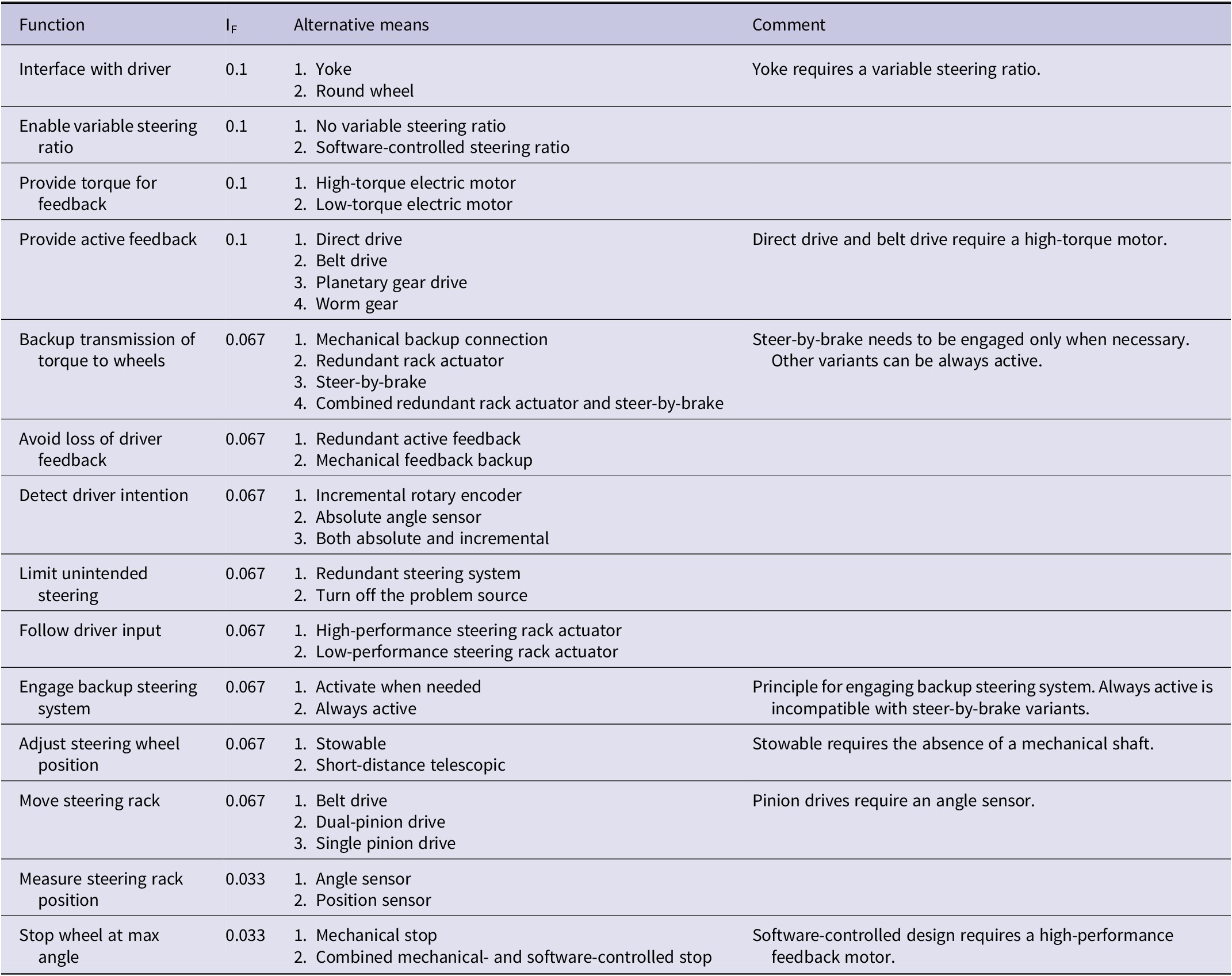
. This was done by having the experts, together with the authors, rate each function on a scale from 1 to 3, where 1 was the least important and 3 was the most important. Those ratings were then normalized over the total sum, resulting in the importance factor of each function. The functions that contained multiple alternative means, along with their importance factor (
$ {I}_{\mathrm{F}} $
. This was done by having the experts, together with the authors, rate each function on a scale from 1 to 3, where 1 was the least important and 3 was the most important. Those ratings were then normalized over the total sum, resulting in the importance factor of each function. The functions that contained multiple alternative means, along with their importance factor ( $ {I}_{\mathrm{F}} $
), are listed in Table 2.
$ {I}_{\mathrm{F}} $
), are listed in Table 2.
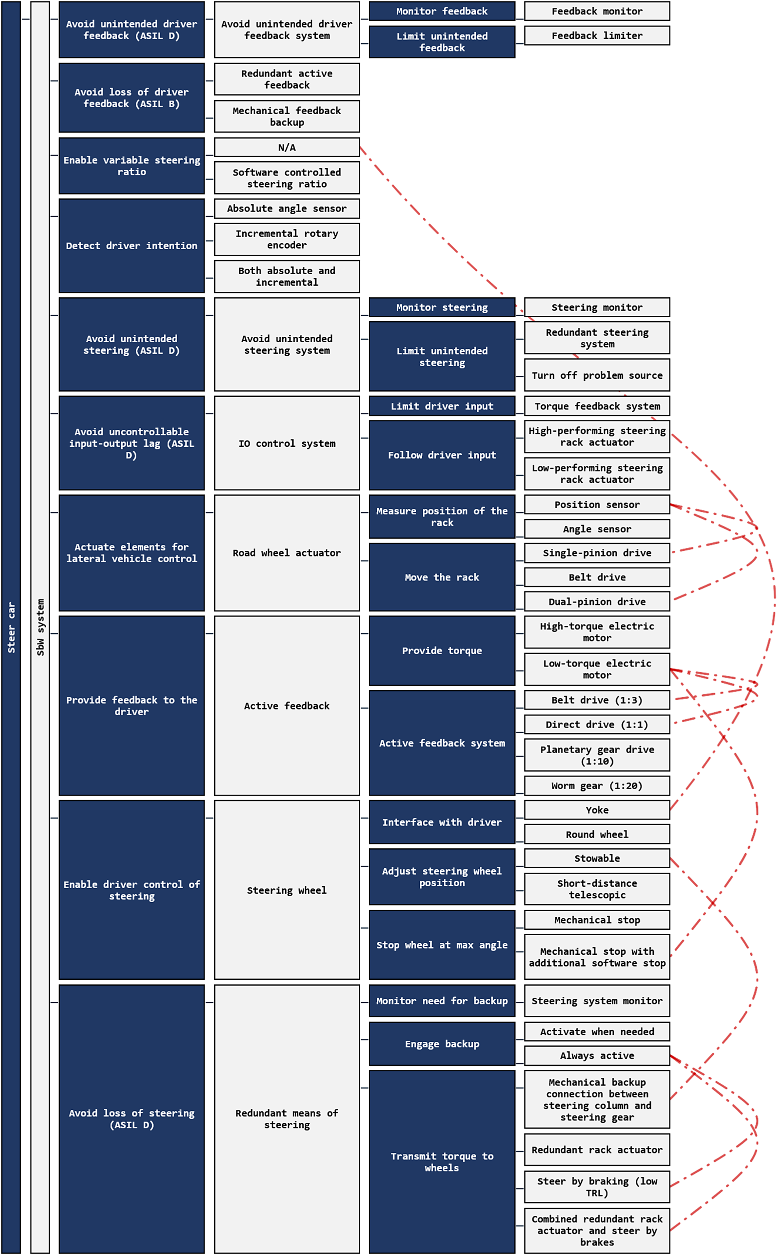
Figure 3. Screenshot of a function-means tree for a steer-by-wire system. The dash-dotted lines that connect some of the means represent incompatibilities.
The incompatibilities were mapped using a DSM that contained all means for all functions. A connection in the DSM between two means indicates that those two means never can be combined. A DSM containing only the incompatible means can be seen in Table 1.
Table 1. DSM containing only the incompatible means. A total of nine incompatibilities were mapped
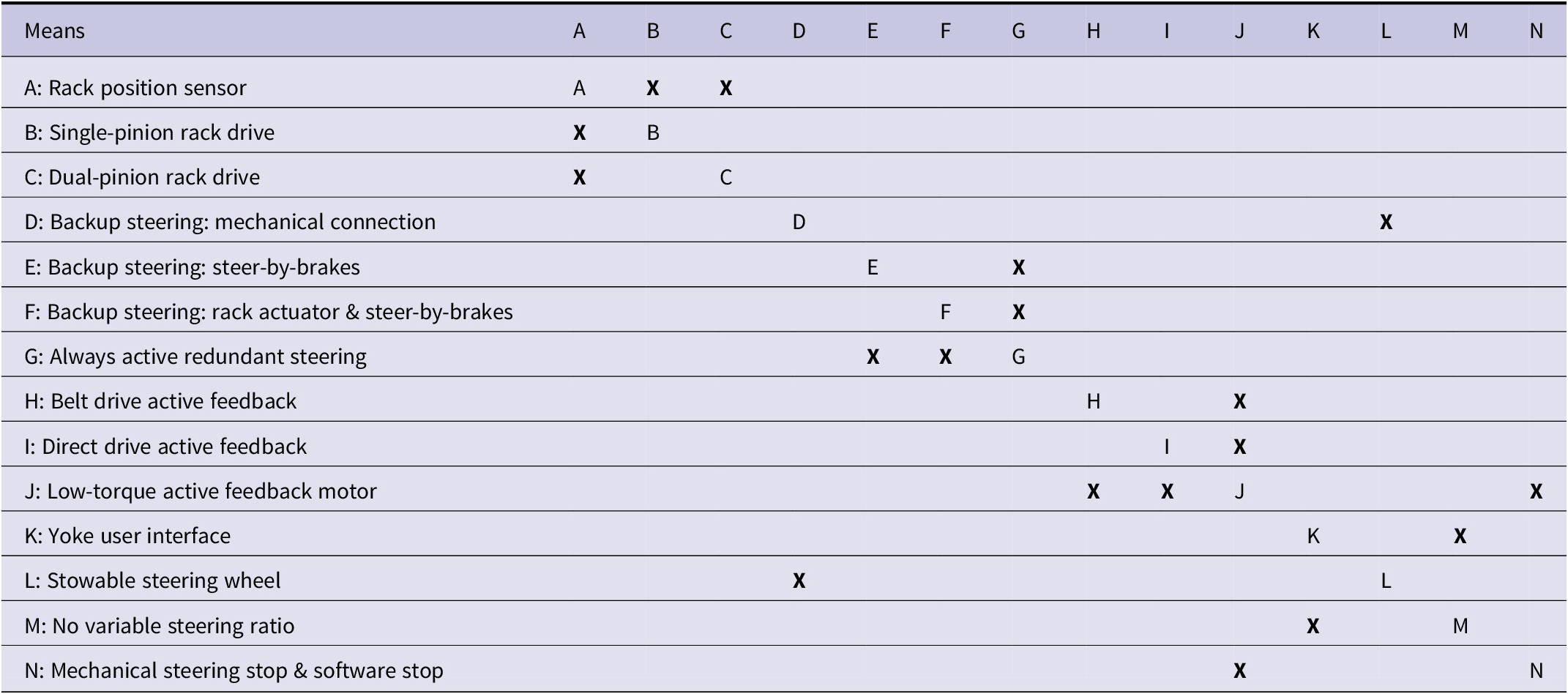
Table 2. System functions for which alternative means were identified and the impact factor ( $ {I}_{\mathrm{F}} $
) of the individual functions
$ {I}_{\mathrm{F}} $
) of the individual functions
Without incompatibilities, the design space spanned $ \mathrm{147,456} $
possible combinations. After applying the incompatibilities using the DSM, that number was reduced to
$ \mathrm{147,456} $
possible combinations. After applying the incompatibilities using the DSM, that number was reduced to $ \mathrm{28,800} $
possible combinations. The next step was to define quantifiable objectives such that this space could be explored using a pathfinding algorithm.
$ \mathrm{28,800} $
possible combinations. The next step was to define quantifiable objectives such that this space could be explored using a pathfinding algorithm.
Implementation of design objectives
Three design objectives were identified: (i) the performance of a component with respect to the functions it fulfills should be maximized; (ii) each component should be as lightweight as possible; and (iii) the cost of the system should be minimized. In practice, safety is the most important factor. However, for this study, it was elected to omit safety as that information is highly sensitive.
To implement performance, weight, and cost ratings into the model, a pairwise comparison was used. For each function, the alternative means available to achieve that function were compared with these three aspects in mind, thus resulting in a score in the range $ \left[0,1\right] $
for each attribute. Additionally, the importance of each function (
$ \left[0,1\right] $
for each attribute. Additionally, the importance of each function ( $ {I}_{\mathrm{F}} $
) was used to determine the impact of any means used to achieve that function when calculating the value of the penalty function. A section of the quantified MM can be seen in Figure 4. The full matrix can be found in the Appendix.
$ {I}_{\mathrm{F}} $
) was used to determine the impact of any means used to achieve that function when calculating the value of the penalty function. A section of the quantified MM can be seen in Figure 4. The full matrix can be found in the Appendix.
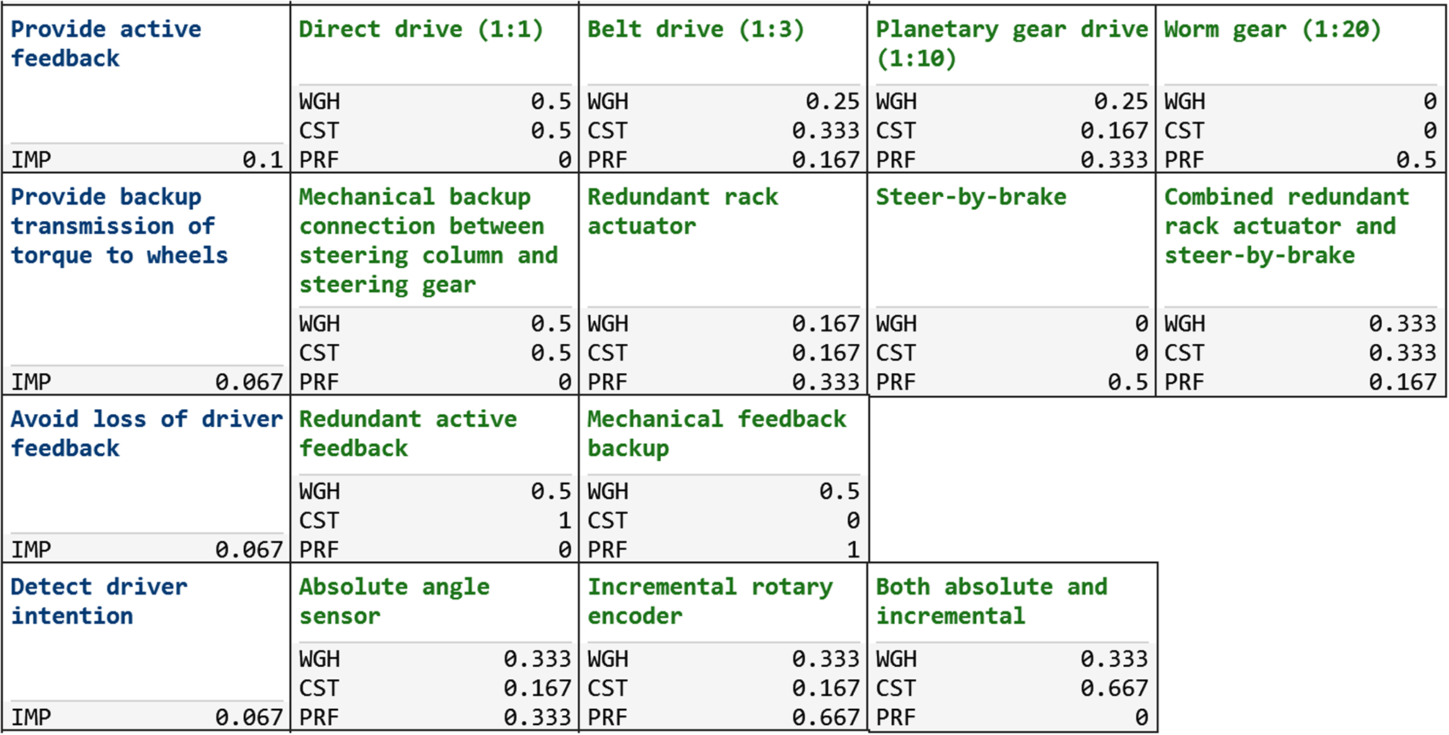
Figure 4. Screenshot of a section of the morphological matrix. It shows the three considered attributes: weight (WGH), cost (CST), and performance (PRF), together with the function importance factor (IMP).
The penalty function (see Equation (3)) was composed as an aggregate of each attribute: weight ( $ w $
), cost (
$ w $
), cost ( $ c $
), and performance (
$ c $
), and performance ( $ p $
) multiplied by the importance of each attribute (
$ p $
) multiplied by the importance of each attribute ( $ {\mathrm{W}}_{\mathrm{w}} $
,
$ {\mathrm{W}}_{\mathrm{w}} $
, $ {\mathrm{W}}_{\mathrm{c}} $
, and
$ {\mathrm{W}}_{\mathrm{c}} $
, and $ {\mathrm{W}}_{\mathrm{p}} $
, representing the importance of design weight, cost, and performance respectively) and summed over all means in a solution candidate (
$ {\mathrm{W}}_{\mathrm{p}} $
, representing the importance of design weight, cost, and performance respectively) and summed over all means in a solution candidate ( $ k $
). The penalty function (
$ k $
). The penalty function ( $ \lambda $
) yields the penalty value of a solution candidate, which determines how well a solution achieves the design objectives. A lower
$ \lambda $
) yields the penalty value of a solution candidate, which determines how well a solution achieves the design objectives. A lower $ \lambda $
value is always preferable. This enabled solutions to be generated for different customer segments. For instance, to generate premium design variants, the cost importance (
$ \lambda $
value is always preferable. This enabled solutions to be generated for different customer segments. For instance, to generate premium design variants, the cost importance ( $ {\mathrm{W}}_{\mathrm{c}} $
) might be reduced while instead allowing for higher-performance importance (
$ {\mathrm{W}}_{\mathrm{c}} $
) might be reduced while instead allowing for higher-performance importance ( $ {\mathrm{W}}_{\mathrm{p}} $
). The values of
$ {\mathrm{W}}_{\mathrm{p}} $
). The values of $ w $
,
$ w $
, $ c $
, and
$ c $
, and $ p $
are determined by the means (
$ p $
are determined by the means ( $ i $
). It should be noted that, since this is a penalty function, lower values are considered to be better, while higher values are penalizing, no matter the metric. Each means achieves a single function, and the importance of that function is represented by an importance factor
$ i $
). It should be noted that, since this is a penalty function, lower values are considered to be better, while higher values are penalizing, no matter the metric. Each means achieves a single function, and the importance of that function is represented by an importance factor $ {I}_{\mathrm{F}i} $
. To calculate the aggregated penalty of a solution candidate, the penalty function sums over all combined means:
$ {I}_{\mathrm{F}i} $
. To calculate the aggregated penalty of a solution candidate, the penalty function sums over all combined means:
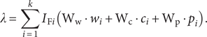 $$ \lambda =\sum \limits_{i=1}^k{I}_{\mathrm{F}i}\left({\mathrm{W}}_{\mathrm{w}}\cdot {w}_i+{\mathrm{W}}_{\mathrm{c}}\cdot {c}_i+{\mathrm{W}}_{\mathrm{p}}\cdot {p}_i\right). $$
To start the solution generation process, the quantified MM and the penalty function were fed to the pathfinding algorithm.
Identifying solution candidates
Three potential customer segments were considered. The first segment, referred to as Premium, is willing to pay extra for high performance. The second segment, Economy, is focused on affordability. The third segment, referred to here as Economy flexible, is an affordable alternative that has the potential to be upgraded. To achieve this, three sets of penalty function objective coefficients were used, as can be seen in Table 3.
Table 3. Penalty function objective coefficients
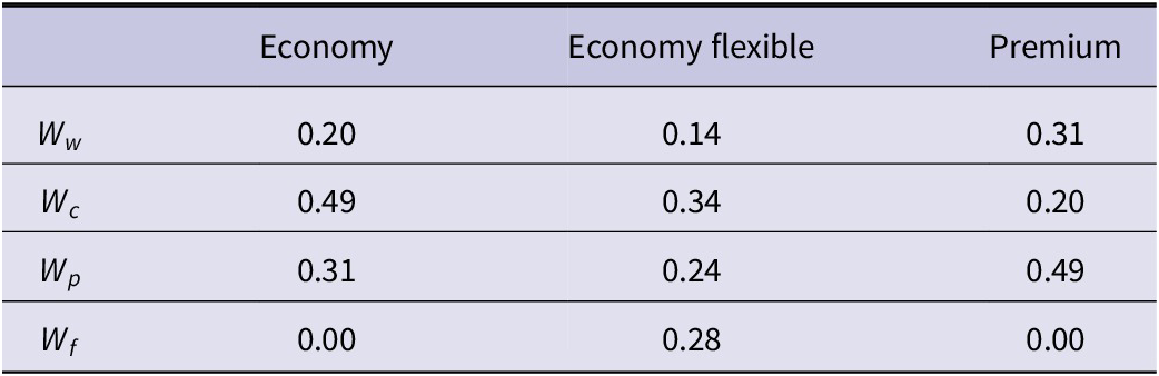
It is desirable for all segments to minimize design weight, as it has a negative effect on energy efficiency. However, the importance of cost and performance naturally varies significantly between the customer segments.
With the penalty function objective coefficients in place, all requirements to execute the pathfinding algorithm were fulfilled. At this point, a decision needed to be made regarding how many solutions to generate. Figure 5 demonstrates how the penalty function, as defined in Equation (3), changes for the $ \mathrm{28,800} $
possible combinations. The change in aggregated solution penalty increases drastically for the first generated solutions and then diminishes slightly. The worst possible solutions are clustered in the end, which results in a final drastic increase in solution penalty.
$ \mathrm{28,800} $
possible combinations. The change in aggregated solution penalty increases drastically for the first generated solutions and then diminishes slightly. The worst possible solutions are clustered in the end, which results in a final drastic increase in solution penalty.
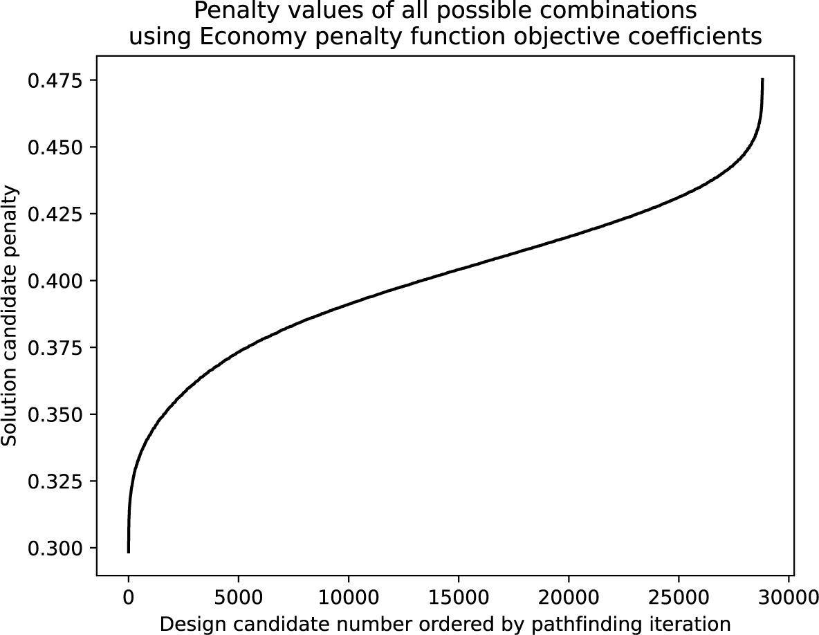
Figure 5. Visualization of how the solution to the penalty function steadily increases with each newly generated solution candidate.
With this in mind, how many solution candidates should be considered? Generating a single solution candidate using pathfinding is a matter of milliseconds; hence, the bottleneck is not computational budget, but engineering capacity. However, the number of solution alternatives that could be efficiently managed within a team of design engineers is outside the scope of this paper. Therefore, for the purposes of this paper, only the solution candidates with the lowest solution penalties per customer segment were considered.
The best-scoring combinations for each segment were, at first glance, reasonable configurations. However, some choices have been made that are nontrivial. For instance, in the Economy variant, the “Belt Drive” was chosen as the means for moving the steering rack, despite being the most expensive alternative. After inspection, there are two reasons for this: (i) the performance benefit of the belt drive and (ii) the cost–benefit of the Position Sensor for measuring the rack position, which is a necessary choice as that particular sensor is incompatible with any of the less expensive pinion drives. Thus, a combination of accounting for the objective functions and the incompatibilities of certain means resulted in a nontrivial selection.
In the premium segment, the pathfinding algorithm elected to use “steer-by-brake” as a backup for transmitting torque to the wheels. This is the least performant of the backup alternatives, although it is compensated for by being the most lightweight alternative and also the cheapest. A similar choice has been made for the function “Limit unintended steering,” for which the algorithm selected “Turn off problem source,” despite the alternative being more performant.
Finally, it is worth noting the Premium choice of driver interface: both the Yoke and the traditional Steering wheel have similar cost and performance, but the yoke only works with variable steering ratio. Since the variable steering ratio is part of the Premium solution, it does not matter in terms of performance, cost, or weight, which means that it is chosen. Thus, both are viable options for the algorithm.
This addresses the solutions made without taking flexibility into consideration. For the final segment Economy flexible, an attempt was made to identify a solution candidate that was both affordable and upgradable.
Including flexibility in the penalty function
The penalty function was modified to include the flexibility metric described in the “Accounting for flexibility” section, as can be seen in Equation (4). As previously explained, this metric is a ratio that represents how much of the design space is screened off due to the selection of a particular means. However, to make it comparable to the other metrics involved in this scenario, the flexibility metric also needed to be scaled. Consequently, the flexibility value for each means was scaled relative to other options available for each function. This scaled flexibility is noted as $ \hat{f} $
. Additionally, the penalty function coefficients (
$ \hat{f} $
. Additionally, the penalty function coefficients ( $ {W}_w $
,
$ {W}_w $
, $ {W}_c $
,
$ {W}_c $
, $ {W}_p $
, and
$ {W}_p $
, and $ {W}_f $
) were reconfigured to account for the high importance of flexibility. The exact values are specified in Table 3:
$ {W}_f $
) were reconfigured to account for the high importance of flexibility. The exact values are specified in Table 3:
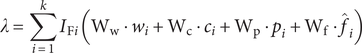 $$ \lambda =\sum \limits_{i=1}^k{I}_{\mathrm{F}i}\left({\mathrm{W}}_{\mathrm{w}}\cdot {w}_i+{\mathrm{W}}_{\mathrm{c}}\cdot {c}_i+{\mathrm{W}}_{\mathrm{p}}\cdot {p}_i+{\mathrm{W}}_{\mathrm{f}}\cdot {\hat{f}}_i\right) $$
These adjustments to the penalty function resulted in a new candidate solution, referred to as Economy flexible. In Table 4, all three candidate solutions are listed, along with the unweighted penalties (without the penalty function objective coefficients) for each of the individual design objectives, and their total penalty value $ \lambda $
. The unweighted penalties provide an overview of how each design candidate performs in each design objective, regardless of variant-specific coefficients. When studying the unweighted penalties, it becomes clear that the Economy variant has the lowest cost penalty (
$ \lambda $
. The unweighted penalties provide an overview of how each design candidate performs in each design objective, regardless of variant-specific coefficients. When studying the unweighted penalties, it becomes clear that the Economy variant has the lowest cost penalty ( $ {\sum}_{i=1}^k\left({I}_{\mathrm{F}i}\cdot {c}_i\right) $
= 0.106), and the Economy flexible and Premium variants have the lowest flexibility (0.033) and performance (0.184) penalties, respectively. The Premium variant has two possible penalty values for unweighted flexibility as it can have either a yoke, which results in a higher flexibility penalty (0.305), since it requires a variable steering ratio, or a wheel. The lowest unweighted penalties for each design objective are shown in bold in Table 4.
$ {\sum}_{i=1}^k\left({I}_{\mathrm{F}i}\cdot {c}_i\right) $
= 0.106), and the Economy flexible and Premium variants have the lowest flexibility (0.033) and performance (0.184) penalties, respectively. The Premium variant has two possible penalty values for unweighted flexibility as it can have either a yoke, which results in a higher flexibility penalty (0.305), since it requires a variable steering ratio, or a wheel. The lowest unweighted penalties for each design objective are shown in bold in Table 4.
Table 4. Optimal choice of means for targeted segments. At the bottom of the table, the total penalty ( $ \lambda $
) of each design candidate is listed, along with the unweighted objective penalties for weight (
$ \lambda $
) of each design candidate is listed, along with the unweighted objective penalties for weight ( $ w $
), cost (
$ w $
), cost ( $ c $
), performance (
$ c $
), performance ( $ p $
), and flexibility (
$ p $
), and flexibility ( $ w $
), summed over all means (
$ w $
), summed over all means ( $ k $
)
$ k $
)
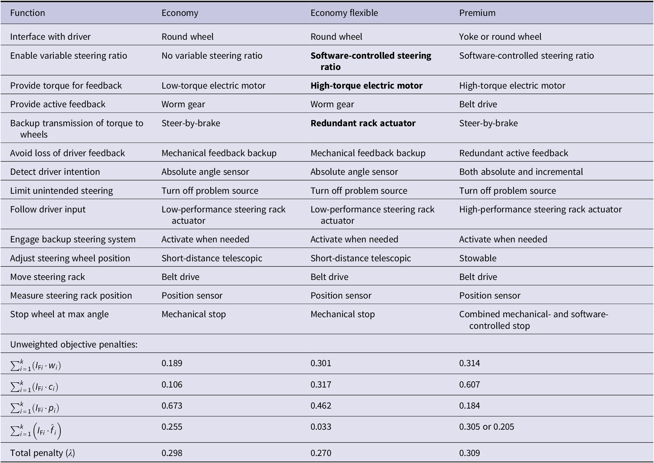
The Economy flexible solution differentiated itself from the Economy variant in three ways, highlighted in bold text in Table 4.
The Economy flexible solution differentiated itself from the Economy variant in three ways, highlighted in bold text in Table 4. The first difference is the software-controlled steering ratio. This means that the system can be changed to have a yoke, which requires a variable steering ratio. The second difference is the provider of torque feedback, for which a high-torque electric motor was selected. This has the benefit of enabling switching to a more high-performing active feedback system such as a belt drive system or a direct drive system. The third difference is the choice of backup transmission of torque to the wheels. Rather than choosing steer-by-braking, as selected in both the Economy and the Premium variants, the flexible variant uses a redundant rack actuator. This was chosen as it enables using the always active backup system, which is not a possibility with the steer-by-braking system.
Ultimately, the aggregated cost of the components of this flexible configuration is likely to be slightly more costly relative to the Economy configuration chosen without flexibility in mind. However, this configuration opens up several paths for upgrading the system and has additional commonalities with the Premium configuration, which can potentially reduce manufacturing and development costs.
Discussion
The discussion is divided into three parts. First, it is key to understand how MOTAC is positioned relative to contemporary research. Other similar methods exist, but none, to the best of our knowledge, handle both discrete design spaces and flexibility using pathfinding. In addition to this, the discussion in the “Relation to existing research” section covers the importance of understanding how these kinds of methods can impact the sustainability of a system. Furthermore, during the development of the MOTAC method, different scenarios were considered, and alternative features of MOTAC were conceptualized. In the “Possible improvements” section, a couple of features are discussed that were left out of the main method to keep the scope clear and focused. Finally, in the “Addressing the research question” section, the research question is discussed.
Relation to the existing research
Using pathfinding algorithms to identify promising solutions is fast and deterministic. The speed comes at the cost of resolution, as more detailed results would require more advanced mathematical models to represent the alternative means. However, as previously argued, in the early phases of design, the mathematical models needed to carry out a conventional optimization are not necessarily available in the early phases of design and may be too resource-intensive to create. Instead, populating means with simpler mathematical models that are based on approximations, or even by relative comparison as in the SbW example, can be used to get an early understanding of the discrete design space. This has precedence in traditional engineering design methodology, where, for instance, Pugh concept selection (Pugh, Reference Pugh1990) often is taught as a means of identifying promising solutions by manually comparing arrays of solutions with each other.
Regarding the use of optimization for concept generation, Pahl et al. (Reference Pahl, Beitz, Feldhusen and Harriman2007) note that optimization or other quantitative methods are “out of place” in the relatively abstract concept phase. However, the authors also state that an exception to this is when the individual elements in the analysis are known. Indeed, MMs can be useful in less abstract scenarios, when more is known about the individual means. An example of this is when supporting product development within a product family, where many of the considered means are likely to have been applied in previous products, or through technology demonstrators. In such scenarios, a lot more is known about the means than in a situation where a completely new product is to be conceived.
Out of the alternative methods identified through the literature review, Ölvander et al. (Reference Ölvander, Lundén and Gavel2009) most closely resemble MOTAC. Thus, it is important to highlight similarities and differences. Similarly to MOTAC, the authors also use a quantified MM, a weighted penalty function, and account for incompatible combinations. However, it uses a different search strategy for identifying combinations, as it uses Tabu Search optimization, unlike MOTAC, which is based on Dijkstra’s algorithm. Tabu search is not guaranteed to avoid local optima, while Dijkstra’s algorithm will always return the best possible combination. On the other hand, Dijkstra’s algorithm is limited to positive penalty function values, which is a restriction that Tabu search does not share. Another small but significant difference can be found in how the MM is quantified. Both methods involve quantifying the properties of each individual means. However, MOTAC also enables quantified properties to be attributed to functions of the system, thus enabling, for instance, functions to be ranked by importance. Finally, the most important difference between the two methods is the inclusion of flexibility metrics in the MOTAC approach.
Furthermore, it is important to discuss how MOTAC relates to design margins. Designing a system that contains excessive capability such that it can accommodate future upgrades can potentially result in overdesign. An example from the examined case in the “Example: Steer-by-wire system” section is the use of a high-torque motor in a car that might not need such a powerful motor. Indeed, it is important to understand the stakeholder needs before committing to a flexible system. Questions such as “Is the system likely to be upgraded?” and “Does the commonality outweigh the losses of excessive margins?” should be asked as early as possible to avoid wasting resources. This is critical from a sustainability perspective, as there is a need to strive to conserve natural resources and minime waste (Benton, Reference Benton2015). In some cases, extending the life of a system can potentially reduce its environmental impact (Vezzoli et al., Reference Vezzoli, Kohtala, Srinivasan, Diehl, Fusakul, Xin and Sateesh2017), and making it easier to upgrade a system is one way of extending its potential life (Khan et al., Reference Khan, Mittal, West and Wuest2018). On the other hand, integrating excessive amounts of margins into a system that has no need for such margins will result in superfluous capacity and a waste of resources (Brahma et al., Reference Brahma, Hallstedt, Wynn and Isaksson2024b).
Possible improvements
Depending on the scenario, it can be interesting to bring in additional steps into the MOTAC method. To keep the scope of the demonstrated method focused, some ideas were not included as part of the method, although they can be integrated if necessary. The first of these additional steps, “property thresholds,” accounts for the possibility of requirement-bound limits for certain properties, such as “maximum power consumption” or “maximum weight.” The second additional step is to run a sensitivity analysis on the results to enable securing a higher degree of confidence in the results.
Property thresholds
In certain scenarios, it may be known in advance that a design is not to exceed a certain threshold value to adhere to requirements. For instance, if the weight of the design is not allowed to be too high, concepts that exceed this limit should not be generated. The pathfinding algorithm can be configured to discard any solution candidate that exceeds the threshold. Consider the pseudocode in Pseudocode 2: if the intention is to avoid solutions that exceed a certain weight threshold, then a check can be implemented before adding new means for the pathfinder to explore. This check can be designed to ensure that the weight of the next means, combined with the currently aggregated weight, is within the threshold. If it is not, then do not add that means to the priority queue.
Two criteria need to be considered before using this approach: (i) the impact on computational expenses and (ii) the need for more detailed mathematical models of each means. Since this change results in more solutions being discarded due to exceeding the threshold, it takes more iterations for the algorithm to find solution candidates. However, the impact on computation is only significant for extremely large design spaces. Of higher significance is the time and knowledge needed to refine the mathematical models of each means to provide a high enough resolution to screen out infeasible designs. In other words, the means need to be represented in such a way that they provide a fairly accurate approximation of, for example, the weight of each mean. In the case of configuring existing subsystems, as when designing for a product family, this is more feasible as experience and data from previous designs can be used to populate the models.
Sensitivity analysis
The understanding of each means, and each generated design candidate, in the early phases of design is highly limited. For this reason, it is impossible to determine which design candidate is the “best” already at this stage. This is especially true in cases where low-resolution mathematical models are used to represent the means, such as in the presented case in the “Example: Steer-by-wire system” section. For this reason, we propose generating multiple design candidates using MOTAC. The more designs that are evaluated, the higher the likelihood of identifying a high-performing design. However, the outcome of the pathfinding algorithm highly depends on how the problem is configured. To understand how sensitive the outcome is to the setup, it is likely to be beneficial to perform a sensitivity analysis. This can, for instance, be done by varying the penalty function objective coefficients and property values using the Monte Carlo method. The speed of the pathfinding algorithm is fast enough to permit such an approach. Naturally, it would take more time to set up the design generation process and analyze the results, as the distributions of properties and objective coefficients would need to be configured. However, performing such a sensitivity analysis may ultimately save time as designers avoid rework.
Addressing the research question
With regard to the research question posed in the Introduction, “How can vast discrete design spaces be explored with respect to design objectives and flexibility?” there are naturally an infinite number of ways to solve this problem. In the “Theoretical background” section, multiple ways of exploring discrete design spaces were covered, and in the “Evaluating and trading for design flexibility” section, we looked at different means of quantifying flexibility. However, we did not find any existing attempts at combining discrete design space exploration with quantified flexibility in the early phases of design.
To enable flexibility metrics at this early stage, we needed to consider the information that was available: Which functions are supposed to be achieved by the design, and what are the known alternatives for achieving those functions? Additionally, it was shown in the “Implementation of design objectives” section that some degree of information regarding the relative characteristics and properties of the different means can also be elicited using expert opinions. With this limited information, how can flexibility be quantified and used to support decision-making? It was found that, by looking at the known alternative means, an expert can determine which means cannot be combined. These incompatibilities can be used to quantify the design space by calculating how much of the design space is screened off when committing to any given means in the MM. To simplify the process of identifying and capturing incompatible means, a DSM was used to visualize and store identified incompatibilities.
The final step was to design an appropriate algorithm for navigating the discrete design space with respect to these new metrics. A pathfinding algorithm was deemed suitable, as an MM can be seen as a node network in which only one direction of travel is possible. This approach is also apt for navigating around incompatible combinations, as incompatible node pairings can easily be stored in a fast-access data structure such as a hash table. Similarly, the impact on flexibility can conveniently be integrated as part of the pathfinding algorithm, allowing it to remember previous incompatibilities such that the same incompatibility is not counted twice, as discussed in the “Accounting for flexibility” section.
Notably, the proposed method necessitates a greater effort in terms of preparation compared to its traditional counterpart. Besides performing a functional decomposition and identifying alternative means, objectives need to be defined and the MM needs to be quantified systematically. However, the efficiency of investigating and reducing the discrete design space down to a feasible number of combinations is significantly improved, as is visualized in Figure 6. Since MOTAC automatically excludes incompatible combinations, the design space is immediately reduced significantly. What is left is quickly navigated by the pathfinding algorithm, which assists in identifying a feasible number of design candidates that are to be further investigated. Overall, the process of going from functional decomposition to a set of design candidates for further investigation is made more efficient.
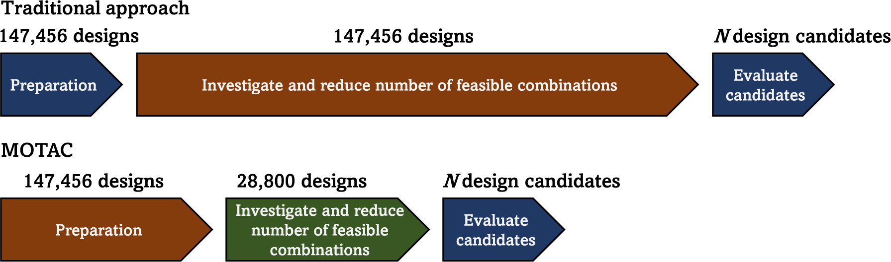
Figure 6. Visualization of how MOTAC improves the efficiency of the design space exploration process. The numbers are based on those identified in the steer-by-wire scenario.
Conclusion
The two key contributions that the MOTAC approach provides are (i) efficiently navigating large discrete design spaces in the form of MMs using a pathfinding algorithm and (ii) involving flexibility in the evaluation of solution candidates when performing discrete design space exploration.
To enable design space exploration using pathfinding, the alternatives in the MM need to be quantifiable. This can be done by identifying objectives that need to be minimized or maximized and attributing each element in the matrix with the necessary information to evaluate those objectives. A penalty function can then be formed, which can be used by a pathfinding algorithm to identify promising design candidates.
Flexibility can be accounted for by mapping which means in the MM are incompatible. This can be captured using a DSM. A pathfinding algorithm can be designed to avoid pairing incompatible combinations while simultaneously measuring how much of an impact this has on the available design space. The more incompatible pairings that are mapped, the more constrained the design space becomes. In this context, flexibility can be thought of as the ratio between the constrained and unconstrained design spaces. We refer to this as combinatorial flexibility, which can be used by a pathfinding algorithm to identify solution candidates that are flexible. In other words, the algorithm can assist in identifying concepts that can be changed, or upgraded, over time.
This approach, combining pathfinding with MMs and flexibility metrics, was designed with two scenarios in mind. The first scenario when this approach can be used is in the early stages of concept development when little is known about the various means. In such a scenario, large MMs can be difficult to explore, and it is often unclear if the most promising designs have been explored. By providing simple objectives based on initial requirements such as minimizing weight or maximizing some aspect of performance, the individual means can be compared and provided with relativistic metrics. This is enough for a pathfinding algorithm to efficiently explore and suggest a predetermined number of solution candidates. In addition, it keeps track of incompatible means and can navigate MMs of sizes that would traditionally be considered as being too large. The second scenario is when designing within a product family. Within a product family, there might already exist a large assortment of technologies that can be combined in various ways. These technologies can be from previous products or from technology development programs. Through the implementation of the flexibility metric, the MOTAC approach can provide strategic support in identifying solution candidates that are compatible with future technology that is not yet ready for market. Thus, contemporary designs can be prepared for the inclusion of novel technologies in the future by ensuring that the designs are compatible with potential future upgrades.
Acknowledgements
The research presented in this paper was funded by the Swedish Innovation Agency (VINNOVA) through the DIFAM 2 project (ID 2023-01196) and the D-SIFT project (ID 2024-03148).
Author contribution
All listed authors have read and approved of the manuscript.
Competing interests
The authors declare that they have no known competing financial interests or personal relationships that could have influenced the work reported in this paper.
Appendix: Steer-by-wire morphological matrix
Figure A1 depicts an MM containing all functions for which there were alternative means in the considered SbW case in the “Example: Steer-by-wire system” section.
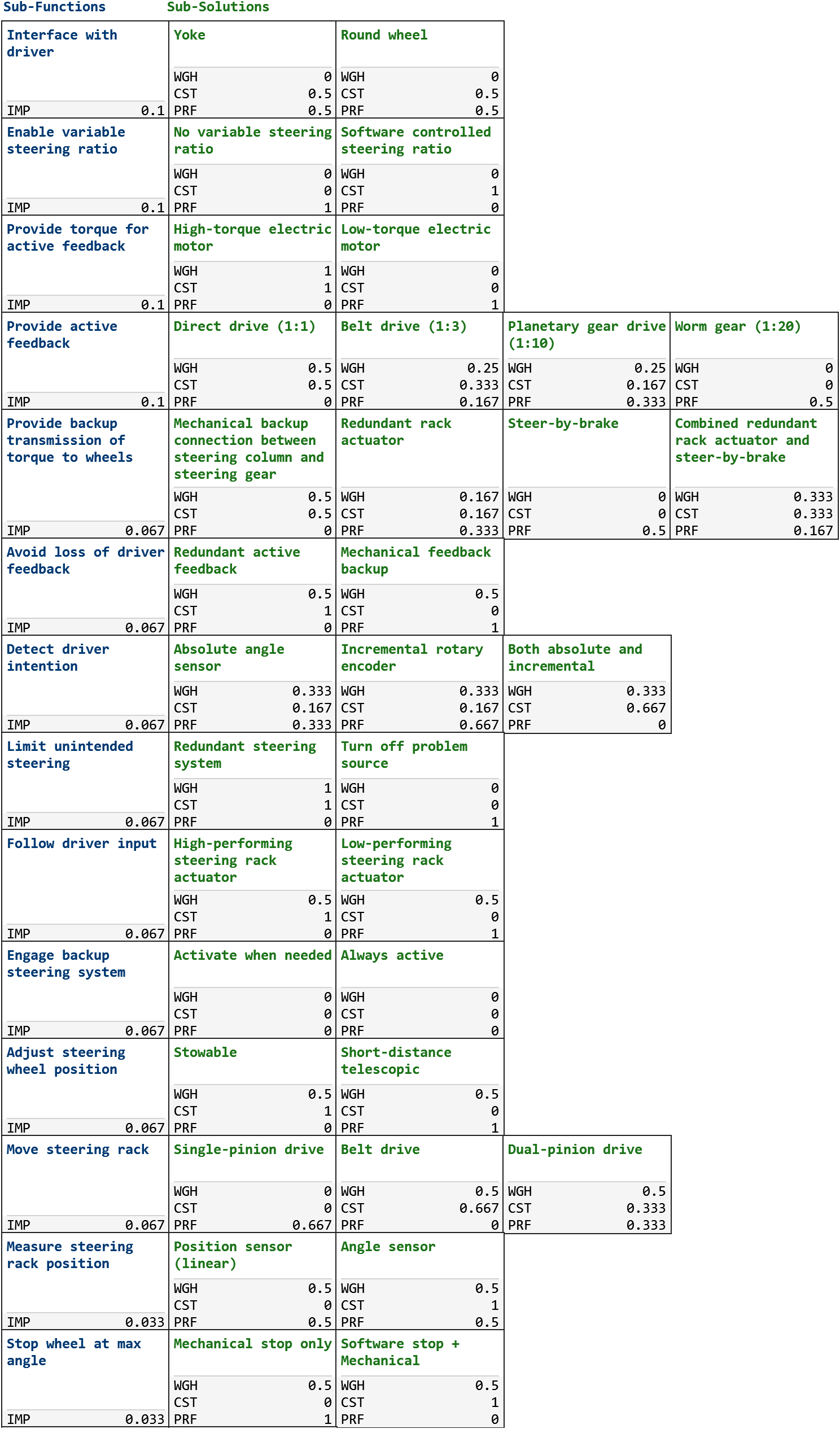
Figure A1. Screenshot of the full morphological matrix for the steer-by-wire system.


 Open access