


1. Introduction
The probabilistic mean value theorem (PMVT) is useful for dealing with differences of means, such as $\mathbb{E}[g(Y)] - \mathbb{E}[g(X)]$
, where X and Y are suitably ordered random variables and g is a given function (cf. Di Crescenzo [Reference Di Crescenzo10]). It has been employed for comparing expectations of conditional random variables, as well as in various applied contexts such as for the estimation of information measures for extreme climate events, for the performance evaluation of algorithms for wireless networks, and for bias estimates in statistical methods (cf. Di Crescenzo and Psarrakos [Reference Di Crescenzo and Psarrakos12] and references therein). See also the recent results on covariance identities for normal and Poisson distributions obtained in Psarrakos [Reference Psarrakos25] by means of the PMVT. However, the need to compare general moments of random variables and their transformations arises in a large variety of applications, including the construction of stochastic orderings for measuring the form of statistical distributions (cf. von Zwet [Reference von Zwet33]), and the variance-based measure of importance for coherent systems with dependent and heterogeneous components proposed by Arriaza et al. [Reference Arriaza, Navarro, Sordo and Suárez-Llorens1].
$\mathbb{E}[g(Y)] - \mathbb{E}[g(X)]$
, where X and Y are suitably ordered random variables and g is a given function (cf. Di Crescenzo [Reference Di Crescenzo10]). It has been employed for comparing expectations of conditional random variables, as well as in various applied contexts such as for the estimation of information measures for extreme climate events, for the performance evaluation of algorithms for wireless networks, and for bias estimates in statistical methods (cf. Di Crescenzo and Psarrakos [Reference Di Crescenzo and Psarrakos12] and references therein). See also the recent results on covariance identities for normal and Poisson distributions obtained in Psarrakos [Reference Psarrakos25] by means of the PMVT. However, the need to compare general moments of random variables and their transformations arises in a large variety of applications, including the construction of stochastic orderings for measuring the form of statistical distributions (cf. von Zwet [Reference von Zwet33]), and the variance-based measure of importance for coherent systems with dependent and heterogeneous components proposed by Arriaza et al. [Reference Arriaza, Navarro, Sordo and Suárez-Llorens1].
Hence, bearing in mind that the variance is clearly essential in several contexts of applied mathematics and statistics, in this paper we aim to use the PMVT to construct suitable forms for the variances of transformed random variables,
 \begin{equation}\mathsf{Var}[g(Y)] - \mathsf{Var}[g(X)].\end{equation}
For instance, the latter terms are useful for connecting the variance of the cumulative weight function with the weighted mean inactivity time function, this leading to possible applications to the lifetime of parallel systems and to the varentropy (namely, the variance of the differential entropy); see, for example, Section 4 of Di Crescenzo and Toomaj [Reference Di Crescenzo and Toomaj13].
Specifically, the sign of a difference as in (1) plays a relevant role in the definition of the reinsurance order. This has been proposed by Denuit and Vermandele [Reference Denuit and Vermandele8] as a tool in reinsurance theory to express the preferences of rational reinsurers when X and Y are two risks to be reinsured and g is a suitable function that describes the reinsurance benefit. In addition, Huang [Reference Huang19] used terms as in (1) for the analysis of variances of maxima of standard Gaussian random variables.
In this paper, stimulated by the research areas and results recalled above, we focus on three main objectives:
-
(i) To obtain relations for $\mathsf{Var}[g(Y)]$
expressed in terms of means of Y, of the equilibrium variable of Y, say
$Y_e$
, and of a suitable 0-inflated version of Y, which will be denoted by
$\tilde Y$
. The aim of this is to disclose similar useful expressions for the difference (1), thanks to the PMVT.
$\mathsf{Var}[g(Y)]$
expressed in terms of means of Y, of the equilibrium variable of Y, say
$Y_e$
, and of a suitable 0-inflated version of Y, which will be denoted by
$\tilde Y$
. The aim of this is to disclose similar useful expressions for the difference (1), thanks to the PMVT. -
(ii) To develop a rigorous approach finalized to express the variance of g(X) in terms of the variance of X. This is based on the construction of a suitable bivariate random vector with ordered components, whose probability density function (PDF) is expressed in terms of the variance of X (cf. Theorem 4 below). The adopted approach leads to exact results that are good alternatives to the approximations provided by the well-known delta method.
-
(iii) To use the above mentioned results in order to compare the variability within pairs of random variables, and to provide consequential applications related to the additive hazards model and to some well-known random variables of interest in actuarial science (such as the per-payment, the per-payment residual loss, and the per-loss residual loss).


The main tools adopted in this investigation refer to typical notions of reliability theory and survival analysis, such as the mean residual lifetime and the mean inactivity time, as well as to customary stochastic orderings. It is worth pointing out that the developments set out in this paper lead us to the following interesting by-product: (a) the definition of a new notion, the ‘centred mean residual lifetime’ (CMRL), that is a suitable modification of the mean residual lifetime; and (b) the introduction of a new related stochastic order based on the comparison of two instances of such a function. In particular, in the main result about the new centred mean residual lifetime (CMRL) order we show that the usual stochastic order and the CMRL order imply that (1) is non-negative for all increasing convex functions g, this leading to the so-called stochastic-variability order (cf. Shaked and Shanthikumar [Reference Shaked and Shanthikumar27] or Belzunce et al. [Reference Belzunce, Suárez-Llorens and Sordo6]).
We recall that the PMVT has been developed also in the setting of discrete random variables (see Section 7 of [Reference Di Crescenzo10]) making use of a discrete version of the equilibrium operator. In the final part of this paper we also present a similar construction for the analysis of the variances of transformed random variables, as in (1), where the underlying equilibrium variables are based on the discrete version of the equilibrium operator. It is worth mentioning that, similarly to general case, even in the case of the discrete transformation we can obtain a suitable expression of the variance of g(X) in terms of the variance of X. This is done by means of a similar discrete bivariate random vector whose probability function is given in terms of the difference between the variance and the Gini mean semi-difference of X (cf. Theorem 14 below).
The paper is organized as follows. Section 2 is focused on using the PMVT to provide suitable expressions for the difference given in (1) and for the variance of a transformed random variable. The latter case is also investigated by adopting an alternative strategy (cf. Section 2.1). Auxiliary results on related probability distributions are shown in Section 2.2. Section 3 introduces and studies the centred version of the mean residual lifetime, this leading to the new CMRL order (see Section 3.1). In addition, in Section 3.2 we apply the previous results to the additive hazards model. Section 4 concerns some applications in actuarial science. Indeed, we provide insights into certain well-known random variables of interest in risk management for financial and insurance industries. Then, in Section 5, the results given in Section 2 are extended to the case of discrete random variables and discrete equilibrium distributions. Finally, some concluding remarks are provided in Section 6.
Throughout the paper, the terms ‘increasing’ and ‘decreasing’ are used in a non-strict sense. We adopt the notation $\mathbb N_0=\mathbb N \cup \{0\}$
,
$\mathbb N_0=\mathbb N \cup \{0\}$
, $\mathbb{R}^+=(0, +\infty)$
and
$\mathbb{R}^+=(0, +\infty)$
and $\mathbb{R}^+_0=[0, +\infty)$
. For any
$\mathbb{R}^+_0=[0, +\infty)$
. For any $x\in \mathbb R$
, the positive part of x is denoted by
$x\in \mathbb R$
, the positive part of x is denoted by $(x)_+=\max\{x,0\}$
. Also, we denote by
$(x)_+=\max\{x,0\}$
. Also, we denote by $g'$
the derivative of any function
$g'$
the derivative of any function $g\colon \mathbb R\to \mathbb R$
. We use
$g\colon \mathbb R\to \mathbb R$
. We use $\mathbf{1}_{A}$
to describe the indicator function,
$\mathbf{1}_{A}$
to describe the indicator function, $\mathbf{1}_{A}=1$
if A is true, and
$\mathbf{1}_{A}=1$
if A is true, and $\mathbf{1}_{A}=0$
otherwise. Moreover,
$\mathbf{1}_{A}=0$
otherwise. Moreover, $X \stackrel{d}{=} Y$
means that X and Y are identically distributed.
$X \stackrel{d}{=} Y$
means that X and Y are identically distributed.
2. Comparison results
Given a probability space $(\Omega, {\mathcal F},\mathbb P)$
, let
$(\Omega, {\mathcal F},\mathbb P)$
, let $Y\colon \Omega\to \mathbb R_0^+$
be a non-negative random variable, with cumulative distribution function (CDF)
$Y\colon \Omega\to \mathbb R_0^+$
be a non-negative random variable, with cumulative distribution function (CDF) $F_Y (x)= \mathbb P(Y\leq x)$
,
$F_Y (x)= \mathbb P(Y\leq x)$
, $x\in \mathbb R_0^+$
, and survival function (SF)
$x\in \mathbb R_0^+$
, and survival function (SF) $\overline{F}_Y (x) = 1-F_Y (x)$
. In addition, if Y has finite non-zero mean
$\overline{F}_Y (x) = 1-F_Y (x)$
. In addition, if Y has finite non-zero mean ${\mathbb{E}} (Y)$
, we can introduce the equilibrium (residual-lifetime) random variable corresponding to Y, say
${\mathbb{E}} (Y)$
, we can introduce the equilibrium (residual-lifetime) random variable corresponding to Y, say $Y_e$
, having CDF
$Y_e$
, having CDF
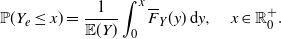 \begin{equation} \mathbb{P}(Y_e \leq x) = \frac{1}{{\mathbb{E}} (Y)} \int_0^x \overline{F}_Y (y) \,{\mathrm{d}} y, \quad x\in \mathbb R^+_0.\end{equation}
We recall that $Y_e$
plays a relevant role in renewal theory and in the probabilistic generalization of Taylor’s theorem, expressed as (see Massey and Whitt [Reference Massey and Whitt21] and Lin [Reference Lin20])
$Y_e$
plays a relevant role in renewal theory and in the probabilistic generalization of Taylor’s theorem, expressed as (see Massey and Whitt [Reference Massey and Whitt21] and Lin [Reference Lin20])
 \begin{equation} \mathbb{E} [g(Y)] = g(0) + \mathbb{E} [g'(Y_e)]\, {\mathbb{E}} (Y),\end{equation}
where g is a differentiable function and $g'$
is Riemann integrable such that
$g'$
is Riemann integrable such that $\mathbb{E} [g'(Y_e)]$
is finite. Similarly, we aim to express the variance of g(Y) in a similar way, in terms of expectations involving g,
$\mathbb{E} [g'(Y_e)]$
is finite. Similarly, we aim to express the variance of g(Y) in a similar way, in terms of expectations involving g, $g'$
and
$g'$
and ${\mathbb{E}} (Y)$
. Differently from (3), which involves in addition only the equilibrium random variable
${\mathbb{E}} (Y)$
. Differently from (3), which involves in addition only the equilibrium random variable $Y_e$
, the result concerning
$Y_e$
, the result concerning $\mathsf{Var}[g(Y)]$
will be expressed also in terms of a suitable 0-inflated version of Y, denoted by
$\mathsf{Var}[g(Y)]$
will be expressed also in terms of a suitable 0-inflated version of Y, denoted by $\tilde{Y}$
.
$\tilde{Y}$
.
Theorem 1. If Y is a non-negative random variable with finite non-zero mean ${\mathbb{E}} (Y)$
, then
${\mathbb{E}} (Y)$
, then
 \begin{equation} \mathsf{Var}[g(Y)] = 2 \left \{ {\mathbb{E}} [g'(Y_e)g(Y_e)] - {\mathbb{E}} [g'(Y_e)]\,{\mathbb{E}} [g(\tilde{Y})] \right \} {\mathbb{E}}(Y), \end{equation}
where g is a differentiable function and $g'$
is Riemann integrable such that
$g'$
is Riemann integrable such that ${\mathbb{E}} [g'(Y_e)g(Y_e)]$
and
${\mathbb{E}} [g'(Y_e)g(Y_e)]$
and $\mathbb{E} [g'(Y_e)]$
are finite, and where
$\mathbb{E} [g'(Y_e)]$
are finite, and where $\tilde{Y}\stackrel{d}{=} Y\cdot I$
, with I being an independent Bernoulli random variable with parameter
$\tilde{Y}\stackrel{d}{=} Y\cdot I$
, with I being an independent Bernoulli random variable with parameter $\frac{1}{2}$
, so that its distribution function is
$\frac{1}{2}$
, so that its distribution function is
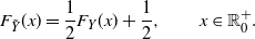 \begin{equation} F_{\tilde{Y}} (x)=\frac{1}{2} F_Y (x) + \frac{1}{2}, \qquad x\in \mathbb R^+_0. \end{equation}
Proof. We apply the probabilistic generalization of Taylor’s theorem (3) for $g^2$
, so that
$g^2$
, so that
 \begin{equation} \mathbb{E} [g^2(Y)] = g^2(0) +2 \,{\mathbb{E}} [g'(Y_e)g(Y_e)] \,{\mathbb{E}} (Y). \end{equation}
Hence, from (3) and (6) we have
 \begin{align*} \mathsf{Var}[g(Y)] =g^2(0) +2 \, {\mathbb{E}} [g'(Y_e)g(Y_e)] \,{\mathbb{E}} (Y) - (g(0) + \mathbb{E} [g'(Y_e)] \,{\mathbb{E}} (Y))^2. \end{align*}
After few calculations we get
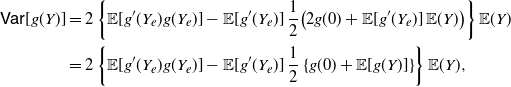 \begin{equation} \begin{split} \mathsf{Var}[g(Y)] & =2 \left \{ {\mathbb{E}} [g'(Y_e)g(Y_e)] - {\mathbb{E}} [g'(Y_e)]\,\frac{1}{2} \big (2g(0) + {\mathbb{E}} [g'(Y_e)] \,{\mathbb{E}} (Y) \big ) \right \} {\mathbb{E}}(Y) \nonumber \\ & = 2 \left \{ {\mathbb{E}} [g'(Y_e)g(Y_e)] -{\mathbb{E}} [g'(Y_e)] \,\frac{1}{2} \left \{g(0) + {\mathbb{E}} [g(Y)] \right \} \right \} {\mathbb{E}}(Y), \end{split} \end{equation}
where the last equality is due to (3). Clearly, for the random variable $\tilde{Y}$
having distribution function (5) one has
$\tilde{Y}$
having distribution function (5) one has
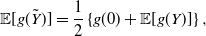 \begin{equation} {\mathbb{E}} [g(\tilde{Y})] = \frac{1}{2} \left \{g(0) + {\mathbb{E}} [g(Y)] \right \}, \end{equation}
so that (4) immediately follows.
Along the lines of Theorem 1, we now aim to construct a suitable representation for the difference of the variances of two random variables. To this end, we recall that, given the random variables X and Y having CDFs ${F}_X(x)$
and
${F}_X(x)$
and ${F}_Y(x)$
, and SFs
${F}_Y(x)$
, and SFs $\overline{F}_X(x)$
and
$\overline{F}_X(x)$
and $\overline{F}_Y(x)$
, respectively, we say that X is smaller than Y in the usual stochastic order, and write
$\overline{F}_Y(x)$
, respectively, we say that X is smaller than Y in the usual stochastic order, and write $X \le_{\mathrm{st}} Y$
, if
$X \le_{\mathrm{st}} Y$
, if ${F}_X(x)\geq {F}_Y(x)$
for all
${F}_X(x)\geq {F}_Y(x)$
for all $x\in \mathbb R$
, or, equivalently, if
$x\in \mathbb R$
, or, equivalently, if $\overline{F}_X(x)\leq \overline{F}_Y(x)$
for all
$\overline{F}_X(x)\leq \overline{F}_Y(x)$
for all $x\in \mathbb R$
(cf. Shaked and Shanthikumar [Reference Shaked and Shanthikumar28]). Let us recall the PMVT given in [Reference Di Crescenzo10].
$x\in \mathbb R$
(cf. Shaked and Shanthikumar [Reference Shaked and Shanthikumar28]). Let us recall the PMVT given in [Reference Di Crescenzo10].
Lemma 1. If X and Y are non-negative random variables such that $X \le_{\mathrm{st}} Y$
and
$X \le_{\mathrm{st}} Y$
and $ \mathbb{E}(X) < \mathbb{E}(Y) <+ \infty$
, then there exists a non-negative absolutely continuous random variable Z having PDF
$ \mathbb{E}(X) < \mathbb{E}(Y) <+ \infty$
, then there exists a non-negative absolutely continuous random variable Z having PDF
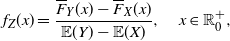 \begin{equation} f_{Z}(x) = \frac{\overline{F}_Y(x) - \overline{F}_X(x)}{\mathbb{E}(Y) - \mathbb{E}(X)}, \quad x\in \mathbb{R}_0^+, \end{equation}
such that
 \begin{equation} \mathbb{E}[g(Y)] - \mathbb{E}[g(X)] = \mathbb{E}[g'(Z)] \, [\mathbb{E}(Y) - \mathbb{E}(X)], \end{equation}
provided that g is a measurable and differentiable function such that $\mathbb{E}[g(X)]$
and
$\mathbb{E}[g(X)]$
and $\mathbb{E}[g(Y)]$
are finite, and that
$\mathbb{E}[g(Y)]$
are finite, and that $g'$
is measurable and Riemann integrable.
$g'$
is measurable and Riemann integrable.
Under the assumptions of Lemma 1, in the following we use the notation $Z \in \mathrm{PMVT}(X,Y)$
to refer to the random variable having PDF (8), which can be viewed as a suitable extension of the equilibrium operator involved in (2) and (3). Indeed, the distribution of
$Z \in \mathrm{PMVT}(X,Y)$
to refer to the random variable having PDF (8), which can be viewed as a suitable extension of the equilibrium operator involved in (2) and (3). Indeed, the distribution of $Z \in$
PMVT(X,Y) can be expressed as a generalized mixture of the equilibrium distributions of X and Y (cf. Section 3 of [Reference Di Crescenzo10]).
$Z \in$
PMVT(X,Y) can be expressed as a generalized mixture of the equilibrium distributions of X and Y (cf. Section 3 of [Reference Di Crescenzo10]).
In Theorem 3 below we present a variance version of the PMVT. Specifically, we aim to express the difference of the variances of equally transformed (stochastically ordered) random variables X and Y as a product of the differences of their means and a term depending on the means of suitable transformations of $Z \in$
PMVT(X,Y) and
$Z \in$
PMVT(X,Y) and $V= {\mathsf{Mix}}_q(X,Y)$
. Here
$V= {\mathsf{Mix}}_q(X,Y)$
. Here $V= {\mathsf{Mix}}_q(X,Y)$
denotes a proper mixture of X and Y such that the distribution function of V is
$V= {\mathsf{Mix}}_q(X,Y)$
denotes a proper mixture of X and Y such that the distribution function of V is
 \begin{align*} {F}_V(x) = q \, {F}_X(x) + (1-q) \, {F}_Y(x), \quad x\in \mathbb R_0^+, \ 0\leq q\leq 1.\end{align*}
Let us first provide a characterization result.
Theorem 2. Let X, V and Y be non-negative random variables such that $X \le_{\mathrm{st}} V \le_{\mathrm{st}} Y$
and
$X \le_{\mathrm{st}} V \le_{\mathrm{st}} Y$
and $ \mathbb{E}(X) < \mathbb{E}(V) < \mathbb{E}(Y) <+ \infty$
, and let
$ \mathbb{E}(X) < \mathbb{E}(V) < \mathbb{E}(Y) <+ \infty$
, and let $Z_1 \in \mathrm{PMVT}(X,Y)$
,
$Z_1 \in \mathrm{PMVT}(X,Y)$
, $Z_2 \in \mathrm{PMVT}(X,V)$
and
$Z_2 \in \mathrm{PMVT}(X,V)$
and $Z_3 \in \mathrm{PMVT}(V,Y)$
. Then, the following equivalence holds:
$Z_3 \in \mathrm{PMVT}(V,Y)$
. Then, the following equivalence holds:
 \begin{equation} V= {\mathsf{Mix}}_q(X,Y) \quad \hbox{for } q=\frac{{\mathbb{E}}(Y)-{\mathbb{E}}(V)}{{\mathbb{E}}(Y)-{\mathbb{E}}(X)} \quad \Leftrightarrow \quad Z_1 \stackrel{d}{=} Z_2 \stackrel{d}{=} Z_3. \end{equation}
Proof. The proof follows after some straightforward calculations.
Recall that, for the absolutely continuous random variables X and Y having respectively PDFs ${f}_X(x)$
and
${f}_X(x)$
and ${f}_Y(x)$
, we say that X is smaller than Y in the likelihood ratio order, and write
${f}_Y(x)$
, we say that X is smaller than Y in the likelihood ratio order, and write $X \le_{\mathrm{lr}} Y$
, if (cf. Shaked and Shanthikumar [Reference Shaked and Shanthikumar28])
$X \le_{\mathrm{lr}} Y$
, if (cf. Shaked and Shanthikumar [Reference Shaked and Shanthikumar28])
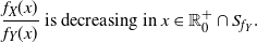 \begin{equation} \frac{{f}_X(x)}{{f}_Y(x)} \ \hbox{is decreasing in $x \in \mathbb R^+_0\cap S_{{f}_Y}$}.\end{equation}
Remark 1. Let X, V and Y be absolutely continuous random variables that satisfy the assumptions of Theorem 2 and such that $X \leq_{\mathrm{lr}}Y$
. If the conditions given in (10) are satisfied, then it is not hard to see that
$X \leq_{\mathrm{lr}}Y$
. If the conditions given in (10) are satisfied, then it is not hard to see that $X \le_{\mathrm{lr}} V \le_{\mathrm{lr}} Y$
.
$X \le_{\mathrm{lr}} V \le_{\mathrm{lr}} Y$
.
Remark 2. Under the assumptions of Theorem 2, if ${\mathbb{E}}(V) = \frac{1}{2} ({\mathbb{E}}(X)+{\mathbb{E}}(Y))$
, then
${\mathbb{E}}(V) = \frac{1}{2} ({\mathbb{E}}(X)+{\mathbb{E}}(Y))$
, then $V= {\mathsf{Mix}}_{1/2}(X,Y)$
.
$V= {\mathsf{Mix}}_{1/2}(X,Y)$
.
The latter case plays a special role in the following result, which is the promised variance version of the PMVT.
Theorem 3. Under the assumptions of Lemma 1, let Z and V be non-negative random variables such that $Z \in \mathrm{PMVT}(X,Y)$
and
$Z \in \mathrm{PMVT}(X,Y)$
and $V= {\mathsf{Mix}}_{1/2}(X,Y)$
. If g is a differentiable function and
$V= {\mathsf{Mix}}_{1/2}(X,Y)$
. If g is a differentiable function and $g'$
is Riemann integrable such that
$g'$
is Riemann integrable such that $\mathbb{E}[g'(Z)g(Z)]$
and
$\mathbb{E}[g'(Z)g(Z)]$
and $\mathbb{E}[g'(Z)]$
are finite, then
$\mathbb{E}[g'(Z)]$
are finite, then
 \begin{equation} \mathsf{Var}[g(Y)] - \mathsf{Var}[g(X)] = 2 \{ {\mathbb{E}} [g'(Z)g(Z)] - {\mathbb{E}}[g'(Z)]\,{\mathbb{E}}[g(V)]\} [{\mathbb{E}} (Y) - {\mathbb{E}} (X)]. \end{equation}
Proof. Applying (9) by using the function $g^2$
instead of g, we obtain
$g^2$
instead of g, we obtain
 \begin{align*} \mathbb{E}[g^2(Y)]-\mathbb{E}[g^2(X)] = 2 \, \mathbb{E}[g'(Z) g(Z) ] \, [\mathbb{E}(Y) - \mathbb{E}(X)]\end{align*}
or, equivalently,
 \begin{equation} \mathsf{Var}[g(Y)]-\mathsf{Var}[g(X)] = 2 \, \mathbb{E}[g'(Z) g(Z) ] \, [\mathbb{E}(Y) - \mathbb{E}(X)] -\{\mathbb{E}[g(Y)]\}^2 +\{\mathbb{E}[g(X)]\}^2.\end{equation}
Making use of (9), we have
 \begin{align*} \{\mathbb{E}[g(Y)]\}^2 -\{\mathbb{E}[g(X)]\}^2 = \mathbb{E}[g'(Z)] \, [\mathbb{E}(Y) - \mathbb{E}(X)] \, \{\mathbb{E}[g(Y)] + \mathbb{E}[g(X)]\},\end{align*}
so that by (13) we get
 \begin{equation} \mathsf{Var}[g(Y)] - \mathsf{Var}[g(X)] = \{2 \, \mathbb{E}[g'(Z) g(Z)] - \mathbb{E}[g'(Z)] \, \{\mathbb{E}[g(X)]+\mathbb{E}[g(Y)]\} \} \, [\mathbb{E}(Y) - \mathbb{E}(X)].\end{equation}
Furthermore, recalling that the CDF of $V= {\mathsf{Mix}}_{1/2}(X,Y)$
is
$V= {\mathsf{Mix}}_{1/2}(X,Y)$
is
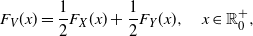 \begin{equation} F_V (x)= \frac{1}{2} F_X (x) + \frac{1}{2} F_Y (x), \quad x\in \mathbb{R}_0^+,\end{equation}
we have
 \begin{align*} \mathbb{E}[g(X)]+\mathbb{E}[g(Y)] = 2 \, \mathbb{E}[g(V)].\end{align*}
Using this identity in (14), we immediately obtain (12), which completes the proof.
Remark 3. We note that, due to case (iv) of Proposition 4.1 of [Reference Di Crescenzo10], one has
-
(i)
$\mathbb{E}(Z)= \mathbb{E}(V)$
if and only if
$\mathsf{Var} (X) = \mathsf{Var} (Y)$
, -
(ii)
$\mathbb{E}(Z) > \mathbb{E}(V)$
if and only if
$\mathsf{Var} (X) < \mathsf{Var} (Y)$
.


Corollary 1. Under the assumption of Theorem 3, if g is an increasing convex (or a decreasing concave) function, then
 \begin{equation} \frac{{\mathsf{Var}} [g(Y)]-{\mathsf{Var}} [g(X)]}{{\mathbb{E}} (Y) -{\mathbb{E}} (X)} \geq 2 \, {\mathbb{E}} [g'(Z)] \left ( {\mathbb{E}} [g(Z)] - {\mathbb{E}} [g(V)]\right )\!.\end{equation}
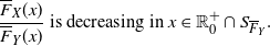
Moreover, if ${\mathbb{E}} [g'(Z)] \not = 0$
, one has
${\mathbb{E}} [g'(Z)] \not = 0$
, one has
 \begin{equation} \frac{{\mathsf{Var}} [g(Y)]-{\mathsf{Var}} [g(X)]}{{\mathbb{E}} [g(Y)] -{\mathbb{E}} [g(X)]} \geq 2 \, \left ( {\mathbb{E}} [g(Z)] - {\mathbb{E}} [g(V)]\right )\!.\end{equation}
Proof. Equation (16) immediately follows from Theorem 3, and noting that if g is an increasing convex (or a decreasing concave) function, then $\mathsf{Cov} (g(Z), g'(Z))= {\mathbb{E}} [g'(Z)g(Z)]- {\mathbb{E}} [g'(Z)] {\mathbb{E}}[g(Z)] \geq 0$
. Also, (17) is obtained by making use of the PMVT in (16).
$\mathsf{Cov} (g(Z), g'(Z))= {\mathbb{E}} [g'(Z)g(Z)]- {\mathbb{E}} [g'(Z)] {\mathbb{E}}[g(Z)] \geq 0$
. Also, (17) is obtained by making use of the PMVT in (16).
In Theorem 3 we expressed the difference of the variances on the left-hand side of (12) as the product of a term depending on Z and V times the difference $\mathbb{E}(Y) - \mathbb{E}(X)$
. We obtain a similar result where the latter difference is replaced by
$\mathbb{E}(Y) - \mathbb{E}(X)$
. We obtain a similar result where the latter difference is replaced by $\mathsf{Var} (Y) - \mathsf{Var} (X)$
.
$\mathsf{Var} (Y) - \mathsf{Var} (X)$
.
Corollary 2. Under the assumptions of Theorem 3, if $\mathsf{Var} (X)\neq \mathsf{Var} (Y)$
then we have
$\mathsf{Var} (X)\neq \mathsf{Var} (Y)$
then we have
 \begin{equation} \mathsf{Var}[g(Y)] - \mathsf{Var}[g(X)] = \bigg \{\frac{ {\mathbb{E}} [g'(Z)g(Z)] - {\mathbb{E}}[g'(Z)]\,{\mathbb{E}}[g(V)]}{{\mathbb{E}} (Z) - {\mathbb{E}} (V)}\bigg \} [\mathsf{Var} (Y) - \mathsf{Var} (X)]. \end{equation}
Proof. By Theorem 3 with $g(x)=x$
, it is easy to see that
$g(x)=x$
, it is easy to see that
 \begin{align*} {\mathbb{E}}(Z)-{\mathbb{E}}(V)=\frac{1}{2} \frac{{\mathsf{Var}} (Y) - {\mathsf{Var}} (X)}{{\mathbb{E}}(Y)-{\mathbb{E}}(X)}.\end{align*}
Hence, by extracting $2 \, [{\mathbb{E}} (Y) - {\mathbb{E}} (X)]$
and using (12), we immediately obtain (18).
$2 \, [{\mathbb{E}} (Y) - {\mathbb{E}} (X)]$
and using (12), we immediately obtain (18).
We remark that if $X=0$
in Theorem 3, then we recover the results given in Theorem 1. Similarly, the following statement follows by Corollary 2 by taking
$X=0$
in Theorem 3, then we recover the results given in Theorem 1. Similarly, the following statement follows by Corollary 2 by taking $X=0$
.
$X=0$
.
Corollary 3. Under the assumption of Lemma 1, if Y is a non-negative random variable with $\mathbb{E} (Y)\in {\mathbb R}^+$
and
$\mathbb{E} (Y)\in {\mathbb R}^+$
and ${\mathsf{Var}} (Y)\in {\mathbb R}^+$
, then
${\mathsf{Var}} (Y)\in {\mathbb R}^+$
, then
 \begin{equation} {\mathsf{Var}}[g(Y)] = \left \{ \frac{ {\mathbb{E}} [g'(Y_e)g(Y_e)] - {\mathbb{E}}[g'(Y_e)]\,{\mathbb{E}}[g(\tilde{Y})]}{{\mathbb{E}} (Y_e) - {\mathbb{E}} (\tilde{Y})}\right \} {\mathsf{Var}} (Y). \end{equation}
Remark 4. From Corollary 3 the terms on the right-hand side of (19) satisfy the inequalities
 \begin{equation} {\mathbb{E}} [g'(Y_e)g(Y_e)] - {\mathbb{E}}[g'(Y_e)]\,{\mathbb{E}}[g(\tilde{Y})]\geq 0, \end{equation}
 \begin{equation} {\mathbb{E}} (Y_e) - {\mathbb{E}} (\tilde{Y}) >0. \end{equation}
Indeed, recalling (2), we have
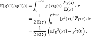 \begin{align*} \begin{split} {\mathbb{E}} [g'(Y_e)g(Y_e)]&=\int_0^{+\infty} g'(x)g(x) \, \frac{\overline{F}_Y (x)}{{\mathbb{E}} (Y)} \,\mathrm{d}x\\ &=\frac{1}{2\,{\mathbb{E}} (Y)} \int_0^{+\infty} [g^2(x)]' \, \overline{F}_Y (x) \,\mathrm{d}x\\ &=\frac{1}{2\,{\mathbb{E}} (Y)} \left ( \mathbb{E}[g^2(Y)] -g^2(0) \right ), \end{split}\end{align*}
where the last equality is obtained by integrating by parts. Furthermore, due to the probabilistic generalization of Taylor’s theorem (3) one has
 \begin{align*} {\mathbb{E}}[g'(Y_e)]\,{\mathbb{E}}[g(\tilde{Y})]=\frac{{\mathbb{E}}[g(Y)]-g(0)}{{\mathbb{E}}(Y)} \, \frac{1}{2} \left \{g(0)+{\mathbb{E}}[g(Y)] \right \} = \frac{1}{2\,{\mathbb{E}} (Y)} \big( \{\mathbb{E}[g(Y)]\}^2-g^2(0) \big). \end{align*}
Hence, (20) is verified if and only if
 \begin{align*} {\mathbb{E}}[g^2(Y)]-g^2(0) \geq \{\mathbb{E}[g(Y)]\}^2-g^2(0) \iff {\mathbb{E}}[g^2(Y)] \geq \{\mathbb{E}[g(Y)]\}^2 \iff {\mathsf{Var}} [g(Y)] \geq 0. \end{align*}
Equation (21) can be obtained similarly for $g(x)=x$
and noting that
$g(x)=x$
and noting that ${\mathsf{Var}} (Y)\in \mathbb R^+$
by assumption.
${\mathsf{Var}} (Y)\in \mathbb R^+$
by assumption.
We note that, differently from the case concerning (19) and treated in Remark 4, the terms appearing in the numerator and in the denominator of the ratio in the curly brackets of (18) may be negative. This occurs, for instance, when X is uniform in (0, 1), Y has a Power distribution with parameter $\alpha =2$
, so that
$\alpha =2$
, so that $X \le_{\mathrm{st}} Y$
, and g is a strictly decreasing function.
$X \le_{\mathrm{st}} Y$
, and g is a strictly decreasing function.
Remark 5. In some applied contexts (see, for example, Sachlas and Papaioannou [Reference Sachlas and Papaioannou26] for instances in actuarial science and survival models) interest lies in non-negative random variables X with an atom at 0, so that $F_X(0) = \mathbb P (X=0)>0$
, and absolutely continuous on
$F_X(0) = \mathbb P (X=0)>0$
, and absolutely continuous on $\mathbb R^+$
. In this case,one has
$\mathbb R^+$
. In this case,one has
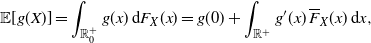 \begin{align*} {\mathbb{E}}[g(X)] =\int_{\mathbb R^+_0} g(x) \, \mathrm{d}F_X(x) = g(0) + \int_{\mathbb R^+} g'(x) \, \overline{F}_X(x) \, \mathrm{d}x,\end{align*}
so that the PMVT can be used, and thus the results given above hold also for random variables of this kind. In this framework, with reference to Theorem 3, the distribution of $Z \in$
PMVT(X,Y) is the same as in (8); moreover,
$Z \in$
PMVT(X,Y) is the same as in (8); moreover, $V= {\mathsf{Mix}}_{1/2}(X,Y)$
has an atom at 0 so that
$V= {\mathsf{Mix}}_{1/2}(X,Y)$
has an atom at 0 so that $\mathbb{P}(V=0)=\frac{1}{2} \,\mathbb{P}(X=0) + \frac{1}{2} \,\mathbb{P}(Y=0)$
.
$\mathbb{P}(V=0)=\frac{1}{2} \,\mathbb{P}(X=0) + \frac{1}{2} \,\mathbb{P}(Y=0)$
.
2.1. Results on
${\mathsf{Var}} [g(X)]$

We recall (see, for instance, Section 2 of Wasserman [Reference Wasserman30]) that the delta method is often applied to approximate the moments of g(X) using Taylor expansions, provided that the function g is sufficiently differentiable and that the moments of X are finite. For instance, if g is differentiable and ${\mathbb{E}}(X^2)$
is finite, estimating the first moment and using a second-order approximation for the random variable X, one obtains
${\mathbb{E}}(X^2)$
is finite, estimating the first moment and using a second-order approximation for the random variable X, one obtains
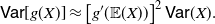 \begin{equation} {\mathsf{Var}}[g(X)] \approx \left[g'({\mathbb{E}}(X))\right]^2 {\mathsf{Var}}(X).\end{equation}
Nevertheless, we can now provide an identity analogous to (22).
Remark 6. Under the assumption of Corollary 3, from Eq. (19) we have
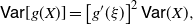 \begin{equation} {\mathsf{Var}}[g(X)] = \left[g'(\xi)\right]^2 {\mathsf{Var}}(X), \end{equation}
where $\xi\in \mathbb R^+$
is such that
$\xi\in \mathbb R^+$
is such that
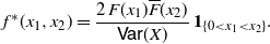
 \begin{equation} [g'(\xi)]^2=\frac{ {\mathbb{E}} [g'(X_e)g(X_e)] - {\mathbb{E}}[g'(X_e)]\,{\mathbb{E}}[g(\tilde{X})]}{{\mathbb{E}} (X_e) - {\mathbb{E}} (\tilde{X})}. \end{equation}
In general, the computation of $\xi$
is not easy. It can be simplified when the inverse of
$\xi$
is not easy. It can be simplified when the inverse of $g'$
exists, and taking Remark 4 into account. Next we provide an example with two cases in which
$g'$
exists, and taking Remark 4 into account. Next we provide an example with two cases in which $\xi$
can be computed analytically.
$\xi$
can be computed analytically.
Example 1. Let X be exponentially distributed with parameter $\lambda\in \mathbb R^+$
, that is, with CDF given by
$\lambda\in \mathbb R^+$
, that is, with CDF given by $F_X(x)=1-e^{-\lambda x}$
,
$F_X(x)=1-e^{-\lambda x}$
, $x\in \mathbb{R}_0^+$
. We recall that
$x\in \mathbb{R}_0^+$
. We recall that ${\mathbb{E}} (X)=1/\lambda$
,
${\mathbb{E}} (X)=1/\lambda$
, ${\mathsf{Var}} (X)=1/\lambda^2$
, and that in this case
${\mathsf{Var}} (X)=1/\lambda^2$
, and that in this case $X \stackrel{d}{=}X_e$
.
$X \stackrel{d}{=}X_e$
.
-
(i) Let
$g(x)=e^x$
, and let
$\lambda>2$
. Then, recalling the moment generating function
${\mathbb{E}} (e^{sX})=\frac{\lambda}{\lambda-s} \mathbf{1}_{\{s<\lambda\}}$
, from (23) and (24) we have since, for
\begin{align*} {\mathsf{Var}} \left (e^X \right )=e^{2\xi}\, {\mathsf{Var}}(X) =\frac{\lambda^3}{(\lambda-1)^2 (\lambda-2)}\, {\mathsf{Var}}(X) =\frac{\lambda}{(\lambda-1)^2 (\lambda-2)},\end{align*}
$\lambda>2$
, we have
$e^{2\xi}=\frac{\lambda^3}{(\lambda-1)^2 (\lambda-2)}$
if and only if
$\xi=\frac{1}{2}\ln \frac{\lambda^3}{(\lambda-1)^2 (\lambda-2)}$
. Note that the approximation in (22) gives
${\mathsf{Var}} \left (e^X \right )\approx e^{\frac{2}{\lambda}}\,{\mathsf{Var}} (X) = \displaystyle\frac{e^{\frac{2}{\lambda}}}{\lambda^2}$
.
-
(ii) Let
$g(x)=\sqrt{x}$
, with
$g'(x)=\frac{1}{2\sqrt{x}}$
. Then the random variables
$\sqrt{X}$
and
$1/\sqrt{X}$
have respectively Weibull and Fréchet distribution, with CDFs
$F_{\sqrt{X}}(x)=1-e^{-\lambda x^2}$
,
$x\in \mathbb{R}_0^+$
, and
$F_{1/\sqrt{X}}(x)=e^{-\lambda x^{-2}}$
,
$x\in \mathbb{R}^+$
, so that Hence, from (23) and (24), after few calculations we obtain
\begin{align*}{\mathbb{E}} \left(\sqrt{X}\right)=\frac{1}{2}\sqrt{\frac{\pi}{\lambda}}, \quad{\mathbb{E}} \left ( \frac{1}{\sqrt{X}} \right )=\sqrt{\lambda\pi}.\end{align*}
with
\begin{align*} {\mathsf{Var}} \left (\sqrt{X}\right )=\frac{1}{4 \xi}\, {\mathsf{Var}}(X) =\lambda \left ( 1-\frac{\pi}{4} \right ) {\mathsf{Var}}(X) =\frac{1}{\lambda} \left ( 1-\frac{\pi}{4} \right ),\end{align*}
$\frac{1}{4 \xi}=\lambda \left ( 1-\frac{\pi}{4} \right )$
, that is to say,
$\xi=\frac{1}{\lambda (4-\pi)}$
, whereas, due to (22), the delta method yields the approximation
${\mathsf{Var}} \left(\sqrt{X}\right)\approx \displaystyle \frac{\lambda}{4} \, {\mathsf{Var}}(X) = \frac{1}{4\lambda}$
.


As seen in (4), Theorem 1 allows us to express the variance of g(X) in terms of the product of the mean of X and a term depending on the random variables $X_e$
and
$X_e$
and $\tilde X$
. This result has been suitably extended in Theorem 3, where the difference
$\tilde X$
. This result has been suitably extended in Theorem 3, where the difference $\mathsf{Var}[g(Y)] - \mathsf{Var}[g(X)]$
is expressed in a similar way. We aim to provide similar decompositions, where the variance of g(X) is given by the product of the variance of X and a suitable mean.
$\mathsf{Var}[g(Y)] - \mathsf{Var}[g(X)]$
is expressed in a similar way. We aim to provide similar decompositions, where the variance of g(X) is given by the product of the variance of X and a suitable mean.
Remark 7. Let X be a non-negative random variable, and let $g\colon \mathbb{R}_0^+\times \mathbb{R}_0^+\to \mathbb{R}$
be a Riemann integrable function, such that
$g\colon \mathbb{R}_0^+\times \mathbb{R}_0^+\to \mathbb{R}$
be a Riemann integrable function, such that $\mathsf{Var}\left[ \int_0^{+\infty} g (X, \theta) \,{\mathrm{d}} \theta \right]$
is finite. Then, from the properties of the covariance, we have
$\mathsf{Var}\left[ \int_0^{+\infty} g (X, \theta) \,{\mathrm{d}} \theta \right]$
is finite. Then, from the properties of the covariance, we have
 \begin{align*} \mathsf{Var} \left [ \int_0^{+\infty} g (X, \theta)\, {\mathrm{d}} \theta \right ] = 2 \int_0^{+\infty} {\mathrm{d}} \theta \int_{\theta}^{+\infty}\mathsf{Cov} \left[ g(X,\theta), g(X,\eta) \right]\, {\mathrm{d}} \eta.\end{align*}
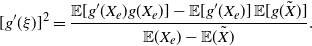
Theorem 4. Let X be a non-negative random variable with CDF F and SF $\overline F$
, such that
$\overline F$
, such that $\mathsf{Var}(X)$
is finite and non-zero. Let g be a differentiable function and let
$\mathsf{Var}(X)$
is finite and non-zero. Let g be a differentiable function and let $g'$
be Riemann integrable such that
$g'$
be Riemann integrable such that ${\mathbb{E}} [ g'(X_1^*) g'(X_2^*)]$
is finite, where
${\mathbb{E}} [ g'(X_1^*) g'(X_2^*)]$
is finite, where $(X_1^*,X_2^*)$
is a non-negative absolutely continuous random vector such that
$(X_1^*,X_2^*)$
is a non-negative absolutely continuous random vector such that $X_1^* \leq X_2^*$
almost surely, having joint PDF
$X_1^* \leq X_2^*$
almost surely, having joint PDF
 \begin{equation} f^* (x_1,x_2)= \frac{2\,F(x_1) \overline{F} (x_2)}{\mathsf{Var}(X)}\, \mathbf{1}_{\{ 0 < x_1 < x_2 \}}. \end{equation}
Then we have
 \begin{equation} \mathsf{Var} [g(X)] = {\mathbb{E}} [ g'(X_1^*) g'(X_2^*)] \,\mathsf{Var} (X).\end{equation}
Proof. Following the probabilistic generalization of Taylor’s theorem (cf. [Reference Massey and Whitt21]), we have
 \begin{align*} \mathsf{Var} [g(X)] = \mathsf{Var} [g(X) - g(0)]= \mathsf{Var} \left [ \int_0^X g' (x) \,{\mathrm{d}} x \right ] = \mathsf{Var} \left [ \int_0^{+\infty} \mathbf{1}_{\{X>x\}} \,g' (x)\, {\mathrm{d}} x \right ].\end{align*}
Hence, making use of Remark 7 and equation (25), it follows that
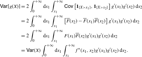 \begin{equation*}\begin{split} \mathsf{Var} [g(X)] = \ & 2 \int_0^{+\infty} {\mathrm{d}} x_1 \int_{x_1}^{+\infty} \mathsf{Cov}\left[ \mathbf{1}_{\{X>x_1\}}, \mathbf{1}_{\{X>x_2\}} \right] g'(x_1) g'(x_2)\, {\mathrm{d}} x_2 \\ = \ &2 \int_0^{+\infty} {\mathrm{d}} x_1 \int_{x_1}^{+\infty} \left[ \overline{F} (x_2) -\overline{F} (x_1) \overline{F} (x_2) \right] g'(x_1) g'(x_2) \,{\mathrm{d}} x_2 \\ = \ &2 \int_0^{+\infty} {\mathrm{d}} x_1 \int_{x_1}^{+\infty} F(x_1) \overline{F} (x_2) g'(x_1) g'(x_2)\, {\mathrm{d}} x_2 \\ = \ &\mathsf{Var} (X) \int_0^{+\infty} {\mathrm{d}} x_1 \int_{x_1}^{+\infty} f^* (x_1,x_2) g'(x_1) g'(x_2)\, {\mathrm{d}} x_2.\end{split}\end{equation*}
Then (26) immediately follows.
Remark 8. Under the assumptions of Theorem 4, by repeated use of Fubini’s theorem and straightforward calculations, one has
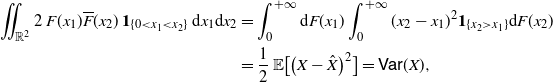 \begin{align} \int\!\!\!\!\int_{\mathbb{R}^2} 2\,F(x_1) \overline{F} (x_2)\,\mathbf{1}_{\{ 0 < x_1 < x_2 \}} \,{\mathrm{d}} x_1{\mathrm{d}} x_2 & = \int_0^{+\infty} \mathrm{d}F (x_1) \int_0^{+\infty} (x_2-x_1)^2 \mathbf{1}_{\{x_2 > x_1\}} {\mathrm{d}} F (x_2) \nonumber \\ &= \frac{1}{2}\, {\mathbb{E}}\big[ \big(X-\hat X\big)^2 \big]=\mathsf{Var}(X), \end{align}
where $\hat X$
is an independent copy of X. Hence, from (25), we have that
$\hat X$
is an independent copy of X. Hence, from (25), we have that $(X_1^*,X_2^*)$
is an honest random vector.
$(X_1^*,X_2^*)$
is an honest random vector.
Identity (27) recalls the analogous relation concerning the Gini’s mean difference of X that, under the same assumptions, is given by (cf. Yitzhaki and Schechtman [Reference Yitzhaki and Schechtman32], for instance)
 \begin{equation} \int_0^{+\infty} 2\,F(x) \overline{F} (x) \,{\mathrm{d}} x = {\mathbb{E}}\big[ \big|X-\hat X\big| \big]=:\mathsf{GMD}(X).\end{equation}
We remark that identity (26) is quite similar to an analogous result shown in Corollary 4.1 of Psarrakos [Reference Psarrakos24], namely $\mathsf{Var} [w(X)] = {\mathbb{E}} [ w'(X_{\tilde w})]\, {\mathbb{E}} [w'(X_{\star})] \,\mathsf{Var}(X)$
, where the distributions of
$\mathsf{Var} [w(X)] = {\mathbb{E}} [ w'(X_{\tilde w})]\, {\mathbb{E}} [w'(X_{\star})] \,\mathsf{Var}(X)$
, where the distributions of $X_{\tilde w}$
and
$X_{\tilde w}$
and $X_{\star}$
are suitably expressed in terms of the distribution of a non-negative absolutely continuous random variable X, and where w is an increasing function.
$X_{\star}$
are suitably expressed in terms of the distribution of a non-negative absolutely continuous random variable X, and where w is an increasing function.
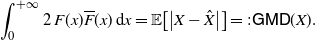
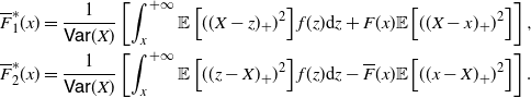
Table 1 shows some examples of densities $f^* (x_1,x_2)$
obtained for suitable choices of the CDF F(x), where
$f^* (x_1,x_2)$
obtained for suitable choices of the CDF F(x), where $\gamma$
and
$\gamma$
and $\Gamma$
denote respectively the lower and upper incomplete gamma functions. Note that the last example considered in Table 1 refers to a case in which X is discrete (i.e., Bernoulli), whereas in all other cases X is absolutely continuous.
$\Gamma$
denote respectively the lower and upper incomplete gamma functions. Note that the last example considered in Table 1 refers to a case in which X is discrete (i.e., Bernoulli), whereas in all other cases X is absolutely continuous.
Table 1. Examples of joint PDFs $f^* (x_1,x_2)$
for some choices of the distribution of X.
$f^* (x_1,x_2)$
for some choices of the distribution of X.
Remark 9. The identity given in (26) can be suitably specialized for suitable choices of g. For instance, if the assumptions of Theorem 4 are satisfied for
(i) $g(x)=x^{\alpha}$
,
$g(x)=x^{\alpha}$
, $\alpha\in [1,+\infty)$
, then
$\alpha\in [1,+\infty)$
, then
 \begin{align*} \mathsf{Var} \big[ X^{\alpha}\big] = \alpha^2\, {\mathbb{E}} \big[ (X_1^* X_2^*)^{\alpha-1}\big] \,\mathsf{Var} (X);\end{align*}
(ii) $g(x)=e^{\beta x}$
,
$g(x)=e^{\beta x}$
, $\beta \in \mathbb{R}^+$
, then
$\beta \in \mathbb{R}^+$
, then
 \begin{align*} \mathsf{Var} \big[e^{\beta X}\big] = \beta^2 \, {\mathbb{E}} \big[e^{\beta (X_1^* + X_2^*)}\big] \,\mathsf{Var} (X).\end{align*}
2.2. Results on the marginal distributions
In this section we study the marginal distributions of $X^*_1$
and
$X^*_1$
and $X^*_2$
. In order to give a probabilistic representation of their PDFs, we recall that, given a non-negative random variable X with SF
$X^*_2$
. In order to give a probabilistic representation of their PDFs, we recall that, given a non-negative random variable X with SF $\overline{F}(x)$
, its stop-loss function is defined as
$\overline{F}(x)$
, its stop-loss function is defined as
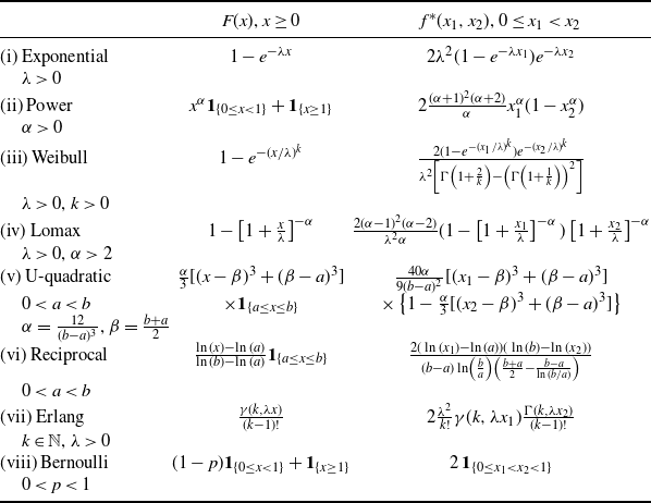
 \begin{equation} \mathbb{E}\left[(X-x)_+\right]=\int_x^{+\infty} \overline{F}(t)\, {\mathrm{d}} t, \quad x\in\mathbb R^+_0.\end{equation}
The stop-loss function is useful in the context of actuarial risks (cf. Section 1.2.2 of Belzunce et al. [Reference Belzunce, Martnez-Riquelme and Mulero5], for instance). It is worth mentioning that in a similar way we can define the reversed stop-loss function of X as
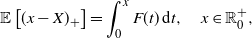 \begin{equation} \mathbb{E}\left[(x-X)_+\right]= \int_0^{x} {F}(t)\, {\mathrm{d}} t, \quad x\in\mathbb R^+_0,\end{equation}
where F is the CDF of X. Clearly, due to (29) and (30), these functions are related by
 \begin{equation*} \mathbb{E}\left[(X-x)_+\right]-\mathbb{E}\left[(x-X)_+\right]=\mathbb{E}\left[X\right]-x, \quad x\in\mathbb R^+_0.\end{equation*}
Corollary 4. (i) Under the assumptions of Theorem 4, the PDFs of $X^*_1$
and
$X^*_1$
and $X^*_2$
are given respectively by
$X^*_2$
are given respectively by
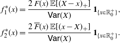 \begin{equation} \begin{split} f_{1}^*(x) &= \frac{2\,F(x)\,{\mathbb{E}} [(X-x)_{+}]}{\mathsf{Var}(X)}\,\mathbf{1}_{\{x \in\mathbb R^+_0 \}}, \\ f_{2}^* (x) &= \frac{2\,\overline{F}(x)\, {\mathbb{E}} [(x-X)_{+}]}{\mathsf{Var}(X)}\,\mathbf{1}_{\{x \in\mathbb R^+_0 \}}.\end{split}\end{equation}
(ii) Moreover, for $x\in\mathbb R^+_0$
the SFs of
$x\in\mathbb R^+_0$
the SFs of $X_1^*$
and
$X_1^*$
and $X_2^*$
can be expressed as
$X_2^*$
can be expressed as
 \begin{equation*} \begin{split} \overline{F}_{1}^*(x) & = \frac{1}{\mathsf{Var}(X)} \left [ \int_x^{+\infty} \mathbb{E} \left [((X-z)_+)^2 \right ] f(z)\mathrm{d}z + F(x) \mathbb{E} \left [ ((X-x)_+)^2 \right ] \right ], \\ \overline{F}_{2}^* (x) & = \frac{1}{\mathsf{Var}(X)} \left [\int_x^{+\infty} \mathbb{E} \left [((z-X)_+)^2 \right ] f(z)\mathrm{d}z -\overline{F}(x) \mathbb{E} \left [ ((x-X)_+)^2 \right ] \right ]. \end{split}\end{equation*}
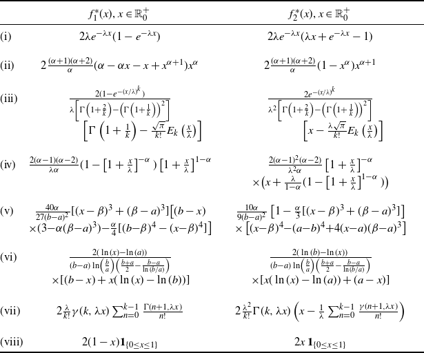
Table 2 shows some examples of the PDFs of $X^*_1$
and
$X^*_1$
and $X^*_2$
provided in (31), where
$X^*_2$
provided in (31), where $E_k(x)=(k! /\sqrt{\pi})\int_0^x e^{-t^k} {\rm d}t$
is the generalized error function, and
$E_k(x)=(k! /\sqrt{\pi})\int_0^x e^{-t^k} {\rm d}t$
is the generalized error function, and ${\rm erf}(x)=E_2(x)$
denotes the Gauss error function. In this table, the PDF
${\rm erf}(x)=E_2(x)$
denotes the Gauss error function. In this table, the PDF $f_1^* (x)$
of case (i) is a special instance of the weighted exponential PDF (see, for instance, Gupta and Kundu [Reference Gupta and Kundu17]).
$f_1^* (x)$
of case (i) is a special instance of the weighted exponential PDF (see, for instance, Gupta and Kundu [Reference Gupta and Kundu17]).
Table 2. PDFs $f_1^* (x)$
and
$f_1^* (x)$
and $f_2^* (x)$
for the examples of Table 1.
$f_2^* (x)$
for the examples of Table 1.
Recalling Proposition 3.9 of Asadi and Berred [Reference Asadi and Berred3], we can express $X_1^*$
and
$X_1^*$
and $X_2^*$
in terms of the equilibrium distribution, the second-order equilibrium distribution and the length-biased distribution of the original random variable X.
$X_2^*$
in terms of the equilibrium distribution, the second-order equilibrium distribution and the length-biased distribution of the original random variable X.
Remark 10. Under the assumptions of Theorem 4, if ${\mathbb{E}} (X_e) \in \mathbb R^+$
, then the random variable
${\mathbb{E}} (X_e) \in \mathbb R^+$
, then the random variable $X_1^*$
can be written as
$X_1^*$
can be written as
 \begin{align*}X_1^* \stackrel{d}{=} [X_{e_2}|X < X_{e_2}],\end{align*}
where $X_{e_2}$
is the second-order equilibrium distribution of X, having PDF
$X_{e_2}$
is the second-order equilibrium distribution of X, having PDF $f_{e_2}(x) = f_{e}(x) / {\mathbb{E}} (X_e)$
, for all
$f_{e_2}(x) = f_{e}(x) / {\mathbb{E}} (X_e)$
, for all $x \in \mathbb R^+$
.
$x \in \mathbb R^+$
.
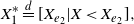
On the other hand, we can write $X_2^*$
as a generalized mixture, given by
$X_2^*$
as a generalized mixture, given by
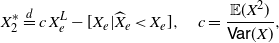 \begin{align*}X_2^* \stackrel{d}{=} c \, X_e^L -[X_e|\widehat{X}_e < X_e],\quad c= \frac{{\mathbb{E}}(X^2)}{{\mathsf{Var}} (X)},\end{align*}
where $X_e^L$
is the length-biased distribution of
$X_e^L$
is the length-biased distribution of $X_e$
, whose PDF is
$X_e$
, whose PDF is $f_e^L (x)=x f_e(x)/{\mathbb{E}} (X_e)$
, and
$f_e^L (x)=x f_e(x)/{\mathbb{E}} (X_e)$
, and $\widehat{X}_e$
is an independent copy of
$\widehat{X}_e$
is an independent copy of $X_e$
.
$X_e$
.
The random variables introduced in Theorem 4 satisfy $X_1^* \leq X_2^*$
almost surely, so that from Theorem 1.A.1 of Shaked and Shanthikumar [Reference Shaked and Shanthikumar28] one immediately has that
$X_1^* \leq X_2^*$
almost surely, so that from Theorem 1.A.1 of Shaked and Shanthikumar [Reference Shaked and Shanthikumar28] one immediately has that $X_1^*$
and
$X_1^*$
and $X_2^*$
are ordered according to the usual stochastic order (see Chapter 1 of [Reference Shaked and Shanthikumar28] for details). Let us now investigate if the stronger relation based on the likelihood ratio order can be established between such random variables. To this end, we adopt the notation
$X_2^*$
are ordered according to the usual stochastic order (see Chapter 1 of [Reference Shaked and Shanthikumar28] for details). Let us now investigate if the stronger relation based on the likelihood ratio order can be established between such random variables. To this end, we adopt the notation $S_G\;:\!=\;\{x\in \mathbb R^+_0\colon G(x)>0\}$
, for any function
$S_G\;:\!=\;\{x\in \mathbb R^+_0\colon G(x)>0\}$
, for any function $G\colon\mathbb R^+_0\to \mathbb R$
.
$G\colon\mathbb R^+_0\to \mathbb R$
.
Remark 11. Under the assumptions of Theorem 4, due to (31), the following identity holds:
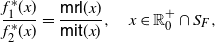 \begin{equation} \frac{f_{1}^*(x)}{f_{2}^* (x)} =\frac{\mathsf{mrl}(x)}{\mathsf{mit}(x)}, \quad x\in\mathbb R^+_0\cap S_{F},\end{equation}
where
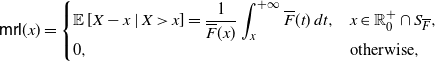 \begin{equation} \mathsf{mrl}(x) = \left\{ \begin{array}{l@{\quad}l} \mathbb{E}\left[X-x \, | \, X > x \right] = \displaystyle\frac{1}{\overline{F}(x)} \int_x^{+\infty} \overline{F}(t) \, {\rm d}t, & x\in\mathbb R^+_0\cap S_{\overline{F}}, \\0, & \hbox{otherwise},\end{array}\right. \end{equation}
and
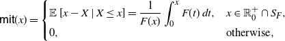 \begin{equation} \mathsf{mit}(x) = \left\{ \begin{array}{l@{\quad}l} \mathbb{E}\left[x-X \, | \, X \le x \right] = \displaystyle \frac{1}{F(x)} \int_0^{x} F(t) \, {\rm d}t, & x\in\mathbb R^+_0 \cap S_{F}, \\0, & \hbox{otherwise},\end{array}\right. \end{equation}
denote respectively the mean residual lifetime and the mean inactivity time of X (see, for instance, Nanda et al. [Reference Nanda, Bhattacharjee and Balakrishnan22] and Section 2 of Navarro [Reference Navarro23]).
If X is a random variable such that its mean residual lifetime and mean inactivity time are increasing, then $X_1^*$
and
$X_1^*$
and $X_2^*$
can be viewed as weighted versions of the equilibrium distribution
$X_2^*$
can be viewed as weighted versions of the equilibrium distribution $X_e$
of X, as we see in the following remark. We recall that, given a random variable X having PDF f, its weighted version
$X_e$
of X, as we see in the following remark. We recall that, given a random variable X having PDF f, its weighted version $X^w$
is a random variable having PDF defined by
$X^w$
is a random variable having PDF defined by
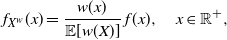 \begin{equation} f_{X^w}(x)=\frac{w(x)}{{\mathbb{E}}[w(X)]}\, f(x), \quad x \in \mathbb{R}^+,\end{equation}
where $w:[0,+\infty)\to [0,+\infty)$
is a continuous function, such that
$w:[0,+\infty)\to [0,+\infty)$
is a continuous function, such that ${\mathbb{E}}[w(X)] \in \mathbb{R}^+$
. This construction modifies the original distribution of X by assigning more weight to certain values according to the function w.
${\mathbb{E}}[w(X)] \in \mathbb{R}^+$
. This construction modifies the original distribution of X by assigning more weight to certain values according to the function w.
Remark 12. Under the assumptions of Theorem 4, if X has finite mean residual lifetime and mean inactivity time, then one has
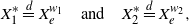 \begin{align*} X_1^* \stackrel{d}{=} X_e^{w_1} \quad \text{and} \quad X_2^* \stackrel{d}{=} X_e^{w_2}, \end{align*}
where $w_1(x)= F(x) \,\mathsf{mrl}(x)$
and
$w_1(x)= F(x) \,\mathsf{mrl}(x)$
and $w_2(x)= F(x)\,\mathsf{mit}(x)$
, for all
$w_2(x)= F(x)\,\mathsf{mit}(x)$
, for all $x\in \mathbb R_0^+ \cap S_{F \cdot \overline{F}}$
.
$x\in \mathbb R_0^+ \cap S_{F \cdot \overline{F}}$
.
Usually, ratios of similar functions involving the mean residual lifetime and the mean inactivity time are encountered in reliability theory and survival analysis when dealing with stochastic orders, relative ageing and similar notions. See, for instance, Finkelstein [Reference Finkelstein16] for the ‘MRL ageing faster’ notion and relative ordering of mean residual lifetime functions, and Arriaza et al. [Reference Arriaza, Sordo and Suárez-Llorens2] for the quantile mean inactivity time order. Quite unexpectedly, the ratio of the marginal densities of $(X_1^*,X_2^*)$
is expressed in (32) as the ratio of
$(X_1^*,X_2^*)$
is expressed in (32) as the ratio of $\mathsf{mrl}(x)$
and
$\mathsf{mrl}(x)$
and $\mathsf{mit}(x)$
, which appears to be new in the literature.
$\mathsf{mit}(x)$
, which appears to be new in the literature.
Identity (32) suggests that we investigate relations between $X_1^*$
and
$X_1^*$
and $X_2^*$
based on the likelihood ratio order and expressed in terms of properties of the functions introduced in (33) and (34). In order to establish a likelihood ratio ordering between
$X_2^*$
based on the likelihood ratio order and expressed in terms of properties of the functions introduced in (33) and (34). In order to establish a likelihood ratio ordering between $X_1^*$
and
$X_1^*$
and $X_2^*$
(see (11)), we recall that for a non-negative absolutely continuous random variable X with PDF f, CDF F and SF
$X_2^*$
(see (11)), we recall that for a non-negative absolutely continuous random variable X with PDF f, CDF F and SF $\overline F$
, the hazard rate and the reversed hazard rate are given respectively by (cf. Navarro [Reference Navarro23] for the main properties and applications of these functions)
$\overline F$
, the hazard rate and the reversed hazard rate are given respectively by (cf. Navarro [Reference Navarro23] for the main properties and applications of these functions)
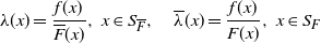 \begin{equation} \lambda(x) = \frac{f(x)}{\overline{F}(x)}, \ x\in S_{\overline F}, \quad \overline{\lambda}(x) = \frac{f(x)}{F(x)}, \ x\in S_{F}\end{equation}
so that $\lambda(x) + \overline{\lambda}(x) =\frac{\lambda(x)}{F(x)}=\frac{\overline{\lambda}(x)}{\overline{F}(x)}$
.
$\lambda(x) + \overline{\lambda}(x) =\frac{\lambda(x)}{F(x)}=\frac{\overline{\lambda}(x)}{\overline{F}(x)}$
.
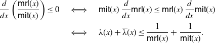
Theorem 5. Under the assumptions of Theorem 4, if X is an absolutely continuous random variable then
 \begin{align*} X_1^* \leq_{\mathrm{lr}} X_2^* \ \text{if and only if} \,\, \lambda(x) + \overline{\lambda}(x) \le \frac{1}{\mathsf{mrl}(x)} + \frac{1}{\mathsf{mit}(x)} \quad \forall\, x\in S_{F\cdot \overline F}.\end{align*}
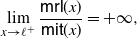
Proof. Due to (33) and (34) we have
 \begin{align*}\lim_{x \to \ell^+} \frac{\mathsf{mrl}(x)}{\mathsf{mit}(x)} = + \infty,\end{align*}
where $\ell=\inf S_{F\cdot \overline F}$
, so that the ratio
$\ell=\inf S_{F\cdot \overline F}$
, so that the ratio $\frac{\mathsf{mrl}(x)}{\mathsf{mit}(x)}$
cannot be increasing in x. Moreover, recalling (36), we have
$\frac{\mathsf{mrl}(x)}{\mathsf{mit}(x)}$
cannot be increasing in x. Moreover, recalling (36), we have
 \begin{equation} \frac{\rm d}{{\rm d}x}\mathsf{mrl}(x) = \lambda(x) \, \mathsf{mrl}(x) - 1, \ \frac{\rm d}{{\rm d}x}\mathsf{mit}(x) =1 - \overline{\lambda}(x) \, \mathsf{mit}(x), \quad x\in S_{F\cdot \overline F}.\end{equation}
and thus
 \begin{align*}\begin{split} \frac{\rm d}{{\rm d}x} \left(\frac{\mathsf{mrl}(x)}{\mathsf{mit}(x)}\right) \le 0 \quad & \iff \quad \mathsf{mit}(x) \, \frac{\rm d}{{\rm d}x} \mathsf{mrl}(x) \le \mathsf{mrl} (x) \,\frac{\rm d}{{\rm d}x} \mathsf{mit}(x) \\ & \iff \quad \lambda(x) + \overline{\lambda}(x) \le \frac{1}{\mathsf{mrl}(x)} + \frac{1}{\mathsf{mit}(x)}.\end{split} \end{align*}
The desired result then follows from identity (32) and condition (11) for $X_1^*$
and
$X_1^*$
and $X_2^*$
.
$X_2^*$
.
Let us now discuss an immediate corollary of Theorem 5, based on suitable monotonicities of the functions $\mathsf{mrl}(x)$
and
$\mathsf{mrl}(x)$
and $\mathsf{mit}(x)$
.
$\mathsf{mit}(x)$
.
Corollary 5. Under the assumptions of Theorem 5, if $\mathsf{mrl}(x)$
is decreasing in
$\mathsf{mrl}(x)$
is decreasing in $x\in S_{F\cdot \overline F}$
(i.e. X is DMRL) and if
$x\in S_{F\cdot \overline F}$
(i.e. X is DMRL) and if $\mathsf{mit}(x)$
is increasing in
$\mathsf{mit}(x)$
is increasing in $x\in S_{F\cdot \overline F}$
(i.e., X is IMIT), then
$x\in S_{F\cdot \overline F}$
(i.e., X is IMIT), then $X_1^* \leq_{\mathrm{lr}} X_2^*$
.
$X_1^* \leq_{\mathrm{lr}} X_2^*$
.
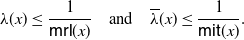
Proof. The monotonicity assumptions of $\mathsf{mrl}(x)$
and
$\mathsf{mrl}(x)$
and $\mathsf{mit}(x)$
, due to (37), imply
$\mathsf{mit}(x)$
, due to (37), imply
 \begin{align*}\lambda(x) \le \frac{1}{\mathsf{mrl}(x)} \quad \mbox{and} \quad \overline{\lambda}(x) \le \frac{1}{\mathsf{mit}(x)}.\end{align*}
Hence, the desired result follows from Theorem 5.
We remark that the ratio $f_1^* (x)/f_2^* (x)$
is decreasing in x, that is,
$f_1^* (x)/f_2^* (x)$
is decreasing in x, that is, $X_1^* \leq_{\mathrm{lr}} X_2^*$
, for all the examples proposed in Table 2. With reference to the distribution of X pertaining to Theorem 4, we note that X is DMRL and IMIT, that is to say, it possesses the properties mentioned in Corollary 5, for the following cases treated in Table 1: (i), (ii) for
$X_1^* \leq_{\mathrm{lr}} X_2^*$
, for all the examples proposed in Table 2. With reference to the distribution of X pertaining to Theorem 4, we note that X is DMRL and IMIT, that is to say, it possesses the properties mentioned in Corollary 5, for the following cases treated in Table 1: (i), (ii) for $\alpha \geq 1$
, (iii), (iv), (vii) and (viii). In case (v), the Lomax random variable has increasing mean residual life and increasing mean inactivity time. Moreover, the mean residual life and the mean inactivity time are non-monotonous for (vi) the U-quadratic distribution and (ii) the power distribution for
$\alpha \geq 1$
, (iii), (iv), (vii) and (viii). In case (v), the Lomax random variable has increasing mean residual life and increasing mean inactivity time. Moreover, the mean residual life and the mean inactivity time are non-monotonous for (vi) the U-quadratic distribution and (ii) the power distribution for $0<\alpha <1$
.
$0<\alpha <1$
.
Let us now discuss a case when the ratio $f_1^* (x)/f_2^* (x)$
is not monotone, whereas
$f_1^* (x)/f_2^* (x)$
is not monotone, whereas $\overline F_1^* (x)/\overline F_2^* (x)$
is decreasing. This suggests that we investigate the relations between
$\overline F_1^* (x)/\overline F_2^* (x)$
is decreasing. This suggests that we investigate the relations between $X_1^*$
and
$X_1^*$
and $X_2^*$
based on a stochastic order that is weaker than the likelihood ratio order. To this end, we recall that if X and Y have SFs
$X_2^*$
based on a stochastic order that is weaker than the likelihood ratio order. To this end, we recall that if X and Y have SFs $\overline F_X(x)$
and
$\overline F_X(x)$
and $\overline F_Y(x)$
, respectively, then X is smaller than Y in the hazard rate order, expressed as
$\overline F_Y(x)$
, respectively, then X is smaller than Y in the hazard rate order, expressed as $X \le_{\mathrm{hr}} Y$
, if
$X \le_{\mathrm{hr}} Y$
, if
 \begin{equation} \frac{\overline F_X(x)}{\overline F_Y(x)} \ \hbox{is decreasing in $x \in \mathbb R^+_0\cap S_{\overline{F}_Y}$}.\end{equation}
Example 2. Let X be a non-negative absolutely continuous random variable having CDF
 \begin{align*}F(x)= e^{-1-\frac{1}{x}} \, \mathbf{1}_{\{0 < x \leq 1 \}} + e^{\frac{x^2-5}{2}} \, \mathbf{1}_{\{1 < x \leq 2\}} + \left [ 1- e^{-(x-2-\ln (1- e^{-1/2}))} \right ] \, \mathbf{1}_{\{ x > 2 \}}\end{align*}
(this is a modification of a CDF treated in Section 2 of Block et al. [Reference Block, Savits and Singh7]). Then it is not hard to show that the assumptions of Theorem 4 are satisfied. Moreover, due to Corollary 4, one has that the ratio $f_1^* (x)/f_2^* (x)$
is not decreasing in
$f_1^* (x)/f_2^* (x)$
is not decreasing in $x\in \mathbb R^+$
, whereas
$x\in \mathbb R^+$
, whereas $\overline F_1^* (x)/\overline F_2^* (x)$
is decreasing in
$\overline F_1^* (x)/\overline F_2^* (x)$
is decreasing in $x\in \mathbb R^+$
(see Figure 1). Hence, recalling (11) and (38), in this case we have
$x\in \mathbb R^+$
(see Figure 1). Hence, recalling (11) and (38), in this case we have $X_1^* \not \le_{\mathrm{lr}} X_2^*$
and
$X_1^* \not \le_{\mathrm{lr}} X_2^*$
and $X_1^* \le_{\mathrm{hr}} X_2^*$
.
$X_1^* \le_{\mathrm{hr}} X_2^*$
.
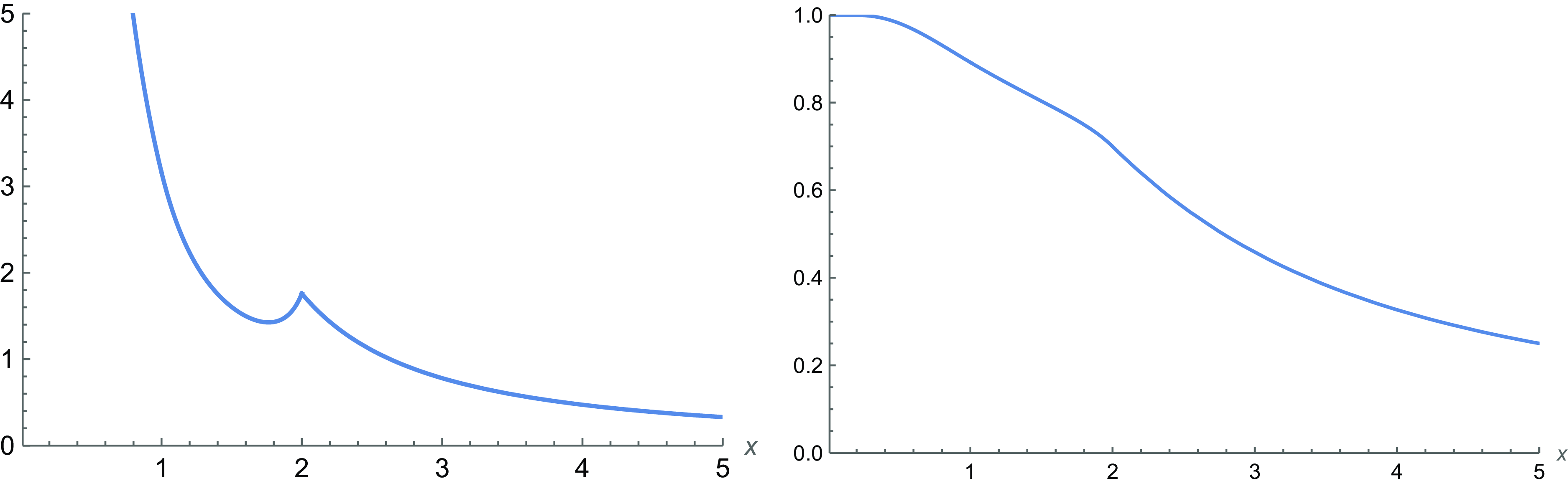
Figure 1. For the case treated in Example 2, a plot of $f_1^* (x)/f_2^* (x)$
(left) and
$f_1^* (x)/f_2^* (x)$
(left) and $\overline F_1^* (x)/\overline F_2^* (x)$
(right).
$\overline F_1^* (x)/\overline F_2^* (x)$
(right).
3. Centred mean residual lifetime and application to additive hazards model
The main aim of this section is to characterize the comparison of variances of transformed pairs of random variables by using the results provided in Section 2. We will also stochastically compare the random variables Z and V considered in Theorem 3. This will require us to introduce a new notion related to the mean residual life. Moreover, we will provide an application to the additive hazards model.
3.1. Centred mean residual lifetime
Let us now recall some stochastic orders and introduce some useful notions. Given two non-negative absolutely continuous random variables X and Y having respectively mean residual lifetimes $\mathsf{mrl}_X(x)$
and
$\mathsf{mrl}_X(x)$
and $\mathsf{mrl}_Y(x)$
defined as in (33), it is well known that X is said to be smaller than Y in the mean residual life order (denoted by
$\mathsf{mrl}_Y(x)$
defined as in (33), it is well known that X is said to be smaller than Y in the mean residual life order (denoted by $X \leq_{\mathrm{mrl}} Y$
) if (see, for instance, Shaked and Shanthikumar [Reference Shaked and Shanthikumar28])
$X \leq_{\mathrm{mrl}} Y$
) if (see, for instance, Shaked and Shanthikumar [Reference Shaked and Shanthikumar28])
 \begin{equation} \mathsf{mrl}_X(x)\leq \mathsf{mrl}_Y(x)\quad \hbox{for all }\textit{x}. \end{equation}
This stochastic order is often used in reliability theory since it provides an effective tool for comparing systems’ reliability. However, since we shall need a modified version of this notion, let us now provide the following definition.
Definition 1. Let X be a non-negative absolutely continuous random variable such that $\mathbb{E}(X)$
is finite. Then we define the centred mean residual lifetime of X as the function
$\mathbb{E}(X)$
is finite. Then we define the centred mean residual lifetime of X as the function
 \begin{equation} \mathsf{cmrl}(x) = \mathsf{mrl}(x) -\mathsf{mrl}(0) = \mathbb{E}\left[X-x \, | \, X>x \right] - \mathbb{E}\left[X\right], \quad x\in\mathbb R^+_0\cap S_{\overline{F}}.\end{equation}
Clearly, the CMRL can be viewed as a measure of positive or negative ageing of X. With this in mind, we recall the following notions (cf. Deshpande et al. [Reference Deshpande, Kochar and Singh9], for instance), for a non-negative random variable X having SF $\overline F(x)$
.
$\overline F(x)$
. $\bullet$
X is new better than used (NBU) if
$\bullet$
X is new better than used (NBU) if $[X-x\, | \, X>x] \leq_{\mathrm{st}} X$
for all
$[X-x\, | \, X>x] \leq_{\mathrm{st}} X$
for all $x\in\mathbb R^+_0\cap S_{\overline{F}}$
or, equivalently, if
$x\in\mathbb R^+_0\cap S_{\overline{F}}$
or, equivalently, if $\overline F(x+t)\leq \overline F(x) \overline F(t)$
for all
$\overline F(x+t)\leq \overline F(x) \overline F(t)$
for all $x,t\in\mathbb R^+_0\cap S_{\overline{F}}$
. Moreover, X is new worse than used (NWU) if the above inequalities are reversed.
$x,t\in\mathbb R^+_0\cap S_{\overline{F}}$
. Moreover, X is new worse than used (NWU) if the above inequalities are reversed.
We also have the following weaker notions of ageing. $\bullet$
X is new better than used in expectation (NBUE) if
$\bullet$
X is new better than used in expectation (NBUE) if $\mathbb{E}[X-x\, | \, X>x] \leq \mathbb{E}[X]$
for all
$\mathbb{E}[X-x\, | \, X>x] \leq \mathbb{E}[X]$
for all $x\in\mathbb R^+_0\cap S_{\overline{F}}$
. Moreover, X is new worse than used in expectation (NWUE) if the above inequality is reversed.
$x\in\mathbb R^+_0\cap S_{\overline{F}}$
. Moreover, X is new worse than used in expectation (NWUE) if the above inequality is reversed.
Remark 13. Due to Definition 1, a non-negative random variable X having SF $\overline F(x)$
is:
$\overline F(x)$
is: $\bullet$
NBUE if and only if
$\bullet$
NBUE if and only if $\mathsf{cmrl}(x) \leq 0$
for all
$\mathsf{cmrl}(x) \leq 0$
for all $x\in\mathbb R^+_0\cap S_{\overline{F}}$
;
$x\in\mathbb R^+_0\cap S_{\overline{F}}$
; $\bullet$
NWUE if and only if
$\bullet$
NWUE if and only if $\mathsf{cmrl}(x) \geq 0$
for all
$\mathsf{cmrl}(x) \geq 0$
for all $x\in\mathbb R^+_0\cap S_{\overline{F}}$
.
$x\in\mathbb R^+_0\cap S_{\overline{F}}$
.
We are now ready to define a new order. In the following, the subscripts refer to the proper random variables.
Definition 2. Let X and Y be non-negative absolutely continuous random variables such that $\mathbb{E}(X)$
and
$\mathbb{E}(X)$
and $\mathbb{E}(Y)$
are finite. We say that X is less than Y in the CMRL order, denoted by
$\mathbb{E}(Y)$
are finite. We say that X is less than Y in the CMRL order, denoted by $X\leq_{\mathrm{cmrl}} Y$
, if
$X\leq_{\mathrm{cmrl}} Y$
, if
 \begin{equation*} \mathsf{cmrl}_X(x) \leq \mathsf{cmrl}_Y(x) \quad \hbox{for all } x\in\mathbb R^+_0\cap S_{\overline{F}_X \cdot \overline{F}_Y}.\end{equation*}
We observe that the relation $X\leq_{\mathrm{cmrl}} Y$
defines a partial stochastic order for suitable equivalence classes. Indeed, the CMRL order given in Definition 2 is reflexive and transitive, but for the antisymmetric property we have the following remark.
$X\leq_{\mathrm{cmrl}} Y$
defines a partial stochastic order for suitable equivalence classes. Indeed, the CMRL order given in Definition 2 is reflexive and transitive, but for the antisymmetric property we have the following remark.
Remark 14. Let X and Y be non-negative absolutely continuous random variables such that $\mathbb{E}(X)$
and
$\mathbb{E}(X)$
and $\mathbb{E}(Y)$
are finite. The relations
$\mathbb{E}(Y)$
are finite. The relations $X\leq_{\mathrm{cmrl}} Y$
and
$X\leq_{\mathrm{cmrl}} Y$
and $Y\leq_{\mathrm{cmrl}} X$
hold simultaneously if and only if
$Y\leq_{\mathrm{cmrl}} X$
hold simultaneously if and only if $\mathsf{mrl}_X(x)-\mathsf{mrl}_Y(x)=k$
for all
$\mathsf{mrl}_X(x)-\mathsf{mrl}_Y(x)=k$
for all $x\in\mathbb R^+_0\cap S_{\overline{F}_X \cdot \overline{F}_Y}$
, where
$x\in\mathbb R^+_0\cap S_{\overline{F}_X \cdot \overline{F}_Y}$
, where $k=\mathbb{E}(Y)-\mathbb{E}(X)$
.
$k=\mathbb{E}(Y)-\mathbb{E}(X)$
.
Example 3. Let $X\sim GP(a,b)$
have generalized Pareto distribution, with SF given by
$X\sim GP(a,b)$
have generalized Pareto distribution, with SF given by
 \begin{align*} \overline{F}_X(x)=\left(\frac{b}{a x + b}\right)^{\frac{1}{a}+1}_+, \quad x\in \mathbb{R}_0^+,\end{align*}
with $a>-1$
,
$a>-1$
, $a\neq 0$
,
$a\neq 0$
, $b>0$
, and where the subscript
$b>0$
, and where the subscript $+$
stands for the positive part of the expression in parentheses. This distribution, which is also known as the Hall–Wellner family, includes the Pareto distribution (for
$+$
stands for the positive part of the expression in parentheses. This distribution, which is also known as the Hall–Wellner family, includes the Pareto distribution (for $a>0$
), the exponential distribution (for
$a>0$
), the exponential distribution (for $a\to 0$
), and the rescaled beta distribution with support
$a\to 0$
), and the rescaled beta distribution with support $[0, -b/a]$
, also known as the power distribution (for
$[0, -b/a]$
, also known as the power distribution (for $-1<a<0$
). Moreover, let
$-1<a<0$
). Moreover, let $Y\sim GP(c,d)$
, with
$Y\sim GP(c,d)$
, with $c>-1$
,
$c>-1$
, $c\neq 0$
,
$c\neq 0$
, $d>0$
. It is well known that the mean residual lifetimes of X and Y are linear, that is,
$d>0$
. It is well known that the mean residual lifetimes of X and Y are linear, that is,
 \begin{align*} \mathsf{mrl}_X(x) = (a\,x+b)_+, \ \mathsf{mrl}_Y(x) = (c\,x+d)_+, \quad x\in \mathbb{R}_0^+.\end{align*} $\bullet$ $X\leq_{\mathrm{mrl}} Y$
if
$X\leq_{\mathrm{mrl}} Y$
if $a\leq c$
and
$a\leq c$
and $b\leq d$
,
$b\leq d$
, $\bullet$ $X\leq_{\mathrm{cmrl}} Y$
if
$X\leq_{\mathrm{cmrl}} Y$
if $a\leq c$
.
$a\leq c$
.
It thus follows that $X\leq_{\mathrm{cmrl}} Y$
and
$X\leq_{\mathrm{cmrl}} Y$
and $Y\leq_{\mathrm{cmrl}} X$
hold simultaneously if
$Y\leq_{\mathrm{cmrl}} X$
hold simultaneously if $a=c$
, irrespective of the values of b and d (cf. Remark 14).
$a=c$
, irrespective of the values of b and d (cf. Remark 14).
Even if the previous example shows a case in which the conditions $X\leq_{\mathrm{mrl}} Y$
and
$X\leq_{\mathrm{mrl}} Y$
and $X\leq_{\mathrm{cmrl}} Y$
may hold simultaneously, in general there are no implications between them, as shown in the following examples.
$X\leq_{\mathrm{cmrl}} Y$
may hold simultaneously, in general there are no implications between them, as shown in the following examples.
Example 4. Let X and Y respectively have exponential distribution with parameter $\lambda>0$
and Lomax distribution with parameters
$\lambda>0$
and Lomax distribution with parameters $\alpha>1$
and
$\alpha>1$
and $\beta>0$
such that
$\beta>0$
such that
 \begin{equation} {\mathbb{E}}(X) = \frac{1}{\lambda} > \frac{\beta}{\alpha-1}= {\mathbb{E}}(Y). \end{equation}
Their survival functions are
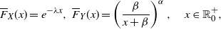 \begin{align*} \overline{F}_X (x)= e^{-\lambda x} , \ \overline{F}_Y (x) = \left(\frac{\beta}{x+\beta}\right)^{\alpha}, \quad x\in \mathbb{R}_0^+,\end{align*}
so that the respective hazard rates are
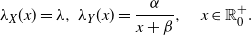 \begin{align*} \lambda_X (x)= \lambda, \ \lambda_Y (x) = \frac{\alpha}{x+\beta}, \quad x\in \mathbb{R}_0^+.\end{align*}
Under assumption (41) we have $ \lambda_X (0) = \lambda < \frac{\alpha}{\beta}= \lambda_Y (0) $
, so that
$ \lambda_X (0) = \lambda < \frac{\alpha}{\beta}= \lambda_Y (0) $
, so that $\lim_{x \rightarrow +\infty} \lambda_X (x) > \lim_{x \rightarrow +\infty} \lambda_Y (x)$
, and thus
$\lim_{x \rightarrow +\infty} \lambda_X (x) > \lim_{x \rightarrow +\infty} \lambda_Y (x)$
, and thus $X \nleq _{\mathrm{hr}} Y$
. On the other hand, recalling (33) and (40), we have, respectively,
$X \nleq _{\mathrm{hr}} Y$
. On the other hand, recalling (33) and (40), we have, respectively,
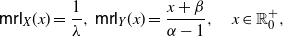 \begin{align*}\begin{split} \mathsf{mrl}_X (x) = \frac{1}{\lambda}, \, \mathsf{mrl}_Y (x) = \frac{ x+\beta}{\alpha-1}, \quad x \in \mathbb{R}_0^+,\end{split}\end{align*}
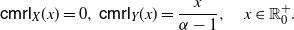 \begin{align*}\begin{split} \mathsf{cmrl}_X (x) = 0, \, \mathsf{cmrl}_Y (x) = \frac{x}{\alpha-1}, \quad x \in \mathbb{R}_0^+.\end{split}\end{align*}
Hence, from Definition 2, one has $X \leq _{\mathrm{cmrl}} Y$
. Moreover, from (39) and (41) it follows that
$X \leq _{\mathrm{cmrl}} Y$
. Moreover, from (39) and (41) it follows that $X \not\leq _{\mathrm{mrl}} Y$
. In conclusion, this example shows that, in general,
$X \not\leq _{\mathrm{mrl}} Y$
. In conclusion, this example shows that, in general,
 \begin{align*} X \leq _{\mathrm{cmrl}} Y \, \nRightarrow \, X \leq _{\mathrm{hr}} Y \quad \hbox{and} \quad X \leq _{\mathrm{cmrl}} Y \, \nRightarrow \, X \leq _{\mathrm{mrl}} Y.\end{align*}
Example 5. Assume that X is exponentially distributed with parameter 1, and Y is Erlang distributed with scale 1 and shape 2, so that $X \leq _{\mathrm{st}} Y$
. Since
$X \leq _{\mathrm{st}} Y$
. Since $\mathsf{mrl}_X (x) = 1$
and
$\mathsf{mrl}_X (x) = 1$
and $\mathsf{mrl}_Y (x) = \frac{ x+2}{x+1}$
,
$\mathsf{mrl}_Y (x) = \frac{ x+2}{x+1}$
, $x \in \mathbb{R}_0^+$
, we have
$x \in \mathbb{R}_0^+$
, we have $X \leq _{\mathrm{mrl}} Y$
. Furthermore, one has
$X \leq _{\mathrm{mrl}} Y$
. Furthermore, one has
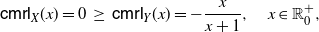 \begin{align*} \mathsf{cmrl}_X (x) = 0 \;\geq \; \mathsf{cmrl}_Y (x) = - \frac{ x}{x+1}, \quad x \in \mathbb{R}_0^+,\end{align*}
and thus $Y \leq _{\mathrm{cmrl}} X$
. This shows that, in general,
$Y \leq _{\mathrm{cmrl}} X$
. This shows that, in general,
 \begin{align*} X \leq _{\mathrm{st}} Y \, \nRightarrow \, X \leq _{\mathrm{cmrl}} Y \quad \hbox{and} \quad X \leq _{\mathrm{mrl}} Y \, \nRightarrow \, X \leq _{\mathrm{cmrl}} Y.\end{align*}
Based on the CMRL order introduced in Definition 2, we are now able to compare the random variables Z and V considered in Theorem 3. For this purpose we also recall the following variability order (cf. Shaked and Shanthikumar [Reference Shaked and Shanthikumar27]).
Definition 3. Given the random variables X and Y, we say that X is less than Y in the stochastic-variability order, denoted by $X \le_{\mathrm{st:icx}} Y$
, if
$X \le_{\mathrm{st:icx}} Y$
, if $X \le_{\mathrm{st}} Y$
and if
$X \le_{\mathrm{st}} Y$
and if $\mathsf{Var}(g(X)) \le \mathsf{Var}(g(Y))$
for all increasing convex functions g, provided that the variances exist.
$\mathsf{Var}(g(X)) \le \mathsf{Var}(g(Y))$
for all increasing convex functions g, provided that the variances exist.
As noted in [Reference Shaked and Shanthikumar27], this order allows us to compare variances of functions rather than just expected values, so that it is useful in applications concerning the variability of stochastic systems.
Theorem 6. Let X and Y be non-negative absolutely continuous random variables such that $X \le_{\mathrm{st}} Y$
and
$X \le_{\mathrm{st}} Y$
and $ \mathbb{E}(X) < \mathbb{E}(Y) < +\infty$
. If
$ \mathbb{E}(X) < \mathbb{E}(Y) < +\infty$
. If $X \leq _{\mathrm{cmrl}} Y$
, then the following results hold for the random variables considered in Theorem 3:
$X \leq _{\mathrm{cmrl}} Y$
, then the following results hold for the random variables considered in Theorem 3:
-
(i)
$V \le_{\mathrm{st}} Z$
; -
(ii)
$X \le_{\mathrm{st:icx}} Y$
.


Proof. The assumption $X \leq _{\mathrm{cmrl}} Y$
, due to (40), is equivalent to
$X \leq _{\mathrm{cmrl}} Y$
, due to (40), is equivalent to
 \begin{align*} \mathsf{mrl}_X(x) + \frac{1}{2} \, [\mathbb{E}(Y)-\mathbb{E}(X)] \le \mathsf{mrl}_Y(x) - \frac{1}{2} \, [\mathbb{E}(Y)-\mathbb{E}(X)]\end{align*}
for all $x\in\mathbb R^+_0\cap S_{\overline{F}_X \cdot \overline{F}_Y}$
. Hence, since
$x\in\mathbb R^+_0\cap S_{\overline{F}_X \cdot \overline{F}_Y}$
. Hence, since $\overline{F}_X(x) \leq \overline{F}_Y(x)$
for all x and
$\overline{F}_X(x) \leq \overline{F}_Y(x)$
for all x and $ \mathbb{E}(X) < \mathbb{E}(Y) < +\infty$
by assumptions, for any x we have
$ \mathbb{E}(X) < \mathbb{E}(Y) < +\infty$
by assumptions, for any x we have
 \begin{align*} \overline{F}_X(x) \, \{\mathsf{mrl}_{X}(x) + \frac{1}{2} \, [\mathbb{E}(Y)-\mathbb{E}(X)] \} \le \overline{F}_Y(x) \, \{\mathsf{mrl}_{Y}(x) - \frac{1}{2} \, [\mathbb{E}(Y)-\mathbb{E}(X)] \}\end{align*}
or, equivalently,
 \begin{align*} \frac{1}{2} \, \overline{F}_X(x) + \frac{1}{2} \, \overline{F}_Y(x) \le \frac{\int_x^{+\infty} \overline{F}_Y(t) \, {\rm d}t - \int_x^{+\infty} \overline{F}_X(t) \, {\rm d}t}{\mathbb{E}(Y)-\mathbb{E}(X)}.\end{align*}
Recalling (15) and (8), we get $\overline{F}_V(x) \le \overline{F}_Z(x)$
for any x, which completes the proof of (i).
$\overline{F}_V(x) \le \overline{F}_Z(x)$
for any x, which completes the proof of (i).
Let g be an increasing convex function. Since g and $g'$
are increasing functions, we have
$g'$
are increasing functions, we have
 \begin{equation}\mathsf{Cov}(g'(Z), g(Z)) =\mathbb{E} [g'(Z)g(Z)] - \mathbb{E}[g'(Z)] \, \mathbb{E}[g(Z)]\geq 0.\end{equation}
Moreover, from (i) one has $\mathbb{E}[g(Z)] \ge \mathbb{E}[g(V)]$
. Hence, we obtain
$\mathbb{E}[g(Z)] \ge \mathbb{E}[g(V)]$
. Hence, we obtain
 \begin{align*} \mathbb{E} [g'(Z)g(Z)] \geq \mathbb{E}[g'(Z)] \, \mathbb{E}[g(Z)] \geq \mathbb{E} [g'(Z)] \, \mathbb{E}[g(V)].\end{align*}
This implies that $\mathsf{Var}[g(X)] \leq \mathsf{Var}[g(Y)]$
due to (12) and assumption
$\mathsf{Var}[g(X)] \leq \mathsf{Var}[g(Y)]$
due to (12) and assumption $ \mathbb{E}(X) < \mathbb{E}(Y) < +\infty$
. Statement (ii) thus follows.
$ \mathbb{E}(X) < \mathbb{E}(Y) < +\infty$
. Statement (ii) thus follows.
Example 6. Suppose that X and Y have Lomax distributions (cf. (iv) of Table 1) with parameters $\lambda_1>0,\alpha_1>2$
and
$\lambda_1>0,\alpha_1>2$
and $\lambda_2>0,\alpha_2>2$
, respectively. Let
$\lambda_2>0,\alpha_2>2$
, respectively. Let $\alpha_1 > \alpha_2$
and
$\alpha_1 > \alpha_2$
and $\lambda_1 < \lambda_2$
, so that
$\lambda_1 < \lambda_2$
, so that $X \le_{\mathrm{st}} Y$
and
$X \le_{\mathrm{st}} Y$
and $\mathbb{E}(X) = \frac{\lambda_1}{\alpha_1-1} < \frac{\lambda_2}{\alpha_2-1} = \mathbb{E}(Y)<+\infty$
. Moreover, for all
$\mathbb{E}(X) = \frac{\lambda_1}{\alpha_1-1} < \frac{\lambda_2}{\alpha_2-1} = \mathbb{E}(Y)<+\infty$
. Moreover, for all $x\in\mathbb R^+_0$
we have
$x\in\mathbb R^+_0$
we have
 \begin{align*}\mathsf{cmrl}_{Y}(x)- \mathsf{cmrl}_{X}(x)= \frac{x}{\alpha_2-1} - \frac{x}{\alpha_1-1} \; \geq \; 0,\end{align*}
so that the assumptions of Theorem 6 are satisfied. See Figure Figure 2 for an instance of the relevant SFs in this case.
We can now obtain a lower bound for the ratio of the increment of variances of transformed random variables over the increment of variances. The following result involves the condition $V \leq_{\mathrm{st}} Z$
, which has been exploited in point (i) of Theorem 6. See also case (ii) of Remark 3.
$V \leq_{\mathrm{st}} Z$
, which has been exploited in point (i) of Theorem 6. See also case (ii) of Remark 3.
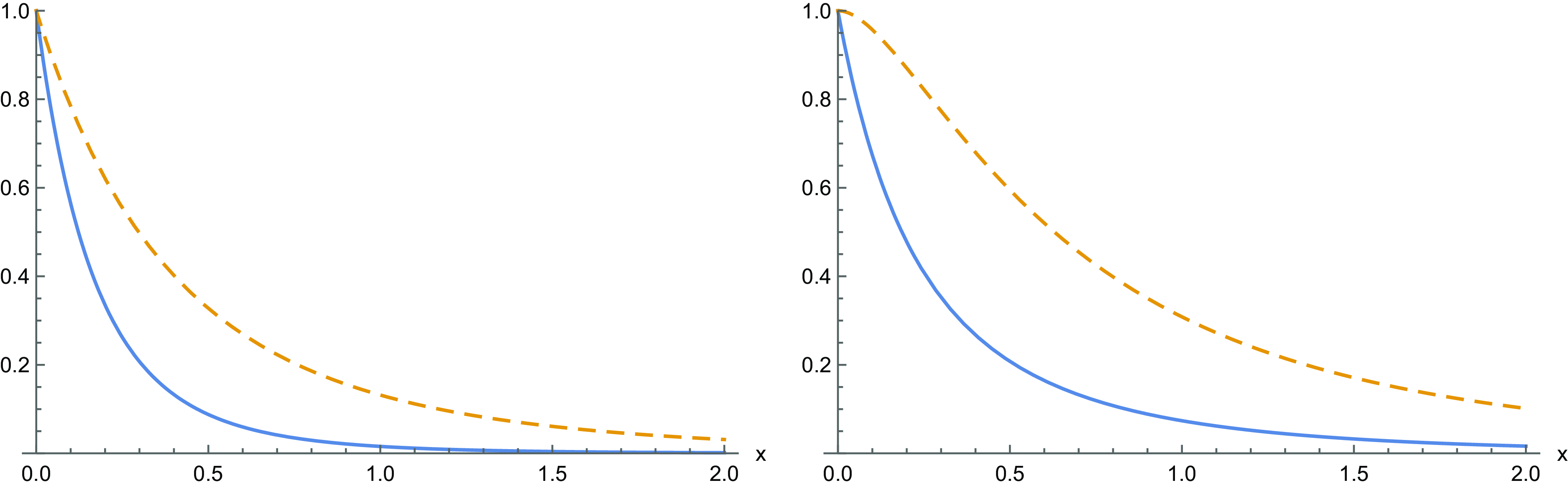
Figure 2. For $\alpha_1=6$
,
$\alpha_1=6$
, $\alpha_2=5$
,
$\alpha_2=5$
, $\lambda_1=1$
and
$\lambda_1=1$
and $\lambda_2=2$
, (left) the survival functions
$\lambda_2=2$
, (left) the survival functions $\overline{F}_X(x)$
(solid line) and
$\overline{F}_X(x)$
(solid line) and $\overline{F}_Y(x)$
(dashed line); (right) the survival functions
$\overline{F}_Y(x)$
(dashed line); (right) the survival functions $\overline{F}_V(x)$
(solid line) and
$\overline{F}_V(x)$
(solid line) and $\overline{F}_Z(x)$
(dashed line).
$\overline{F}_Z(x)$
(dashed line).
Theorem 7. Under the assumptions of Theorem 3, if $\mathsf{Var} (X)< \mathsf{Var} (Y)$
, if
$\mathsf{Var} (X)< \mathsf{Var} (Y)$
, if $V \leq_{\mathrm{st}} Z$
and if g is an increasing convex (or a decreasing concave) function, then
$V \leq_{\mathrm{st}} Z$
and if g is an increasing convex (or a decreasing concave) function, then
 \begin{equation*} \frac{{\mathsf{Var}} [g(Y)] - {\mathsf{Var}} [g(X)]}{{\mathsf{Var}} (Y)-{\mathsf{Var}} (X)} \geq {\mathbb{E}} [g'(Z)] \, {\mathbb{E}} [g'(T)],\end{equation*}
where the random variable $T \in \mathrm{PMVT}(V,Z)$
has PDF
$T \in \mathrm{PMVT}(V,Z)$
has PDF
 \begin{equation} f_T(x)=\frac{\overline{F}_Z(x)-\overline{F}_V(x)}{{\mathbb{E}} (Z) - {\mathbb{E}} (V)},\quad x \in \mathbb R_0^+.\end{equation}
Proof. The proof follows from Corollary 2 and Lemma 1, and making use of (42), so that
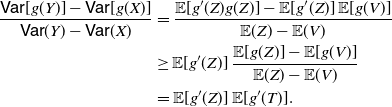 \begin{align*}\begin{split} \frac{{\mathsf{Var}} [g(Y)] - {\mathsf{Var}} [g(X)]}{{\mathsf{Var}} (Y)-{\mathsf{Var}} (X)} & = \frac{ {\mathbb{E}} [g'(Z)g(Z)] - {\mathbb{E}}[g'(Z)]\,{\mathbb{E}}[g(V)]}{{\mathbb{E}} (Z) - {\mathbb{E}} (V)} \\ & \geq {\mathbb{E}}[g'(Z)]\,\frac{ {\mathbb{E}} [g(Z)] - {\mathbb{E}}[g(V)]}{{\mathbb{E}} (Z) - {\mathbb{E}} (V)} \\ & = {\mathbb{E}}[g'(Z)]\, {\mathbb{E}} [g'(T)].\end{split} \end{align*}
The proof is thus complete.
Remark 15. Due to Theorem 7, the PDF given in (43) can be expressed as
 \begin{align*}f_T (x)=2\frac{{\mathbb{E}}[(Y-x)_+]-{\mathbb{E}}[(X-x)_+]}{{\mathsf{Var}} (Y)-{\mathsf{Var}} (X)}-\frac{{\mathbb{E}}(Y) -{\mathbb{E}}(X)}{{\mathsf{Var}} (Y)-{\mathsf{Var}} (X)} \left(\overline{F}_X(x)+\overline{F}_Y(x)\right)\!.\end{align*}
3.2. Additive hazards model
In this section we refer to the additive hazards model (see, for example, Bebbington et al. [Reference Bebbington, Lai and Zitikis4], and Section 6 of Di Crescenzo and Psarrakos [Reference Di Crescenzo and Psarrakos12]). This model, denoted by $(X,Y,\delta)$
-AHM, involves (i) a baseline non-negative absolutely continuous random variable Y having finite mean, survival function
$(X,Y,\delta)$
-AHM, involves (i) a baseline non-negative absolutely continuous random variable Y having finite mean, survival function $\overline{F}_Y(x)$
and hazard rate
$\overline{F}_Y(x)$
and hazard rate $\lambda_Y(x)$
, and (ii) another non-negative absolutely continuous random variable X, whose survival function and hazard rate are given respectively by
$\lambda_Y(x)$
, and (ii) another non-negative absolutely continuous random variable X, whose survival function and hazard rate are given respectively by
 \begin{equation} \overline{F}_{X}(x;\;\delta) = e^{-\delta x} \, \overline{F}_Y(x), \ \lambda_{X}(x;\;\delta) = \lambda_Y(x) + \delta, \quad x\in \mathbb{R}_0^+,\end{equation}
where $\delta > 0$
. From (44) it is clear that
$\delta > 0$
. From (44) it is clear that $X \le_{\mathrm{hr}} Y$
, that is,
$X \le_{\mathrm{hr}} Y$
, that is, $\lambda_{X}(x;\;\delta)\geq \lambda_Y(x)$
for all
$\lambda_{X}(x;\;\delta)\geq \lambda_Y(x)$
for all $x\in \mathbb{R}_0^+$
(cf. Shaked and Shanthikumar [Reference Shaked and Shanthikumar28]). Moreover, recalling (40), we have
$x\in \mathbb{R}_0^+$
(cf. Shaked and Shanthikumar [Reference Shaked and Shanthikumar28]). Moreover, recalling (40), we have
 \begin{equation} \mathsf{cmrl}_{Y}(x) = \mathsf{mrl}_{Y}(x) - \mathbb{E}(Y) = \int_0^{+\infty} \left[\frac{\overline{F}_Y(x+t)}{\overline{F}_Y(x)}- \overline{F}_Y(t) \right] {\rm d}t, \quad x\in \mathbb{R}_0^+\end{equation}
and
 \begin{equation} \mathsf{cmrl}_{X}(x) = \mathsf{mrl}_{X}(x)- \mathbb{E}(X) = \int_0^{+\infty} e^{-\delta t} \left[\frac{\overline{F}_Y(x+t)}{\overline{F}_Y(x)}- \overline{F}_Y(t) \right] {\rm d}t.\end{equation}
For more details, see Section 3 of Bebbington et al. [Reference Bebbington, Lai and Zitikis4]. The given assumptions ensure that the Theorem 3 can be applied; in particular, the survival functions of V and Z are given respectively by
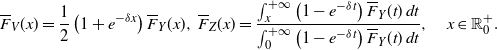 \begin{equation*} \overline{F}_V(x) = \frac{1}{2} \left(1+ e^{-\delta x} \right) \overline{F}_Y(x), \ \overline{F}_Z(x) = \frac{\int_x^{+\infty}\left(1- e^{-\delta t} \right)\overline{F}_Y(t) \, {\rm d}t } {\int_0^{+\infty} \left(1-e^{-\delta t}\right) \overline{F}_Y(t) \, {\rm d}t},\quad x\in \mathbb{R}_0^+.\end{equation*}
Theorem 8 Let X and Y be non-negative absolutely continuous random variables satisfying the $(X,Y,\delta)$
-AHM as specified in (44). If Y is NWU and has finite mean, then
$(X,Y,\delta)$
-AHM as specified in (44). If Y is NWU and has finite mean, then
-
(i)
$V \le_{\mathrm{st}} Z$
, -
(ii)
$X \le_{\mathrm{st:icx}} Y$
.


Proof. Under the $(X,Y,\delta)$
-AHM we have
$(X,Y,\delta)$
-AHM we have $X\le_{\mathrm{hr}}Y$
and thus
$X\le_{\mathrm{hr}}Y$
and thus $X\le_{\mathrm{st}}Y$
. Furthermore, we have
$X\le_{\mathrm{st}}Y$
. Furthermore, we have $\mathbb{E}(X) < \mathbb{E}(Y)<+\infty$
. Hence, from (45) and (46), we obtain
$\mathbb{E}(X) < \mathbb{E}(Y)<+\infty$
. Hence, from (45) and (46), we obtain
 \begin{align*} \mathsf{cmrl}_{Y}(x) -\mathsf{cmrl}_{X}(x) =\int_0^{+\infty} \left(1-e^{-\delta t}\right) \left[\frac{\overline{F}_Y(x+t)}{\overline{F}_Y(x)}- \overline{F}_Y(t) \right] {\rm d}t \geq 0,\end{align*}
where the inequality is due to the assumption that Y is NWU. The results thus follow by Theorem 6.
4. Applications in actuarial science
In this section we focus on some applications in actuarial science, by taking as reference some notions treated in Section 3 of Sachlas and Papaioannou [Reference Sachlas and Papaioannou26]. We assume that X is a non-negative absolutely continuous random variable, having PDF $f_X$
and SF
$f_X$
and SF $\overline{F}_X$
, that describes the losses experienced in an actuarial context after 1 year, and
$\overline{F}_X$
, that describes the losses experienced in an actuarial context after 1 year, and $d>0$
is the deductible value. Clearly, we assume that
$d>0$
is the deductible value. Clearly, we assume that $\overline{F}_X(d)>0$
, and that X possesses finite non-zero first and second moments.
$\overline{F}_X(d)>0$
, and that X possesses finite non-zero first and second moments.
4.1. Per-payment
We now focus on the per-payment defined as
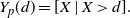 \begin{equation}Y_p(d)=[X\,|\,X>d].\end{equation}
This represents the amount actually paid by the policy, since no benefits are paid to the policyholder if the loss is less than d. Clearly, the PDF and the SF of $Y_p(d)$
are given respectively by
$Y_p(d)$
are given respectively by
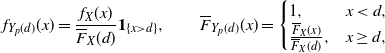 \begin{equation*}f_{Y_p(d)}(x)= \frac{f_X(x)}{\overline{F}_X(d)} \mathbf{1}_{\{x > d\}},\qquad\overline{F}_{Y_p(d)}(x)= \begin{cases} 1, & x < d,\\ \frac{\overline{F}_X(x)}{\overline{F}_X(d)} , & x \geq d,\end{cases}\end{equation*}
so that $X \leq_{\mathrm{st}} Y_p(d)$
. Moreover, recalling (33), one has
$X \leq_{\mathrm{st}} Y_p(d)$
. Moreover, recalling (33), one has
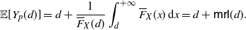 \begin{align*} {\mathbb{E}}[Y_p(d)] = d+\frac{1}{\overline{F}_X (d)} \int_d^{+\infty} \overline{F}_X (x) \,\mathrm{d}x =d+\mathsf{mrl}(d).\end{align*}
Further, due to (40), we have
 \begin{equation}{\mathbb{E}} [Y_p(d)]-{\mathbb{E}} (X)=d+\mathsf{mrl} (d)-{\mathbb{E}}(X)=d+\mathsf{cmrl} (d).\end{equation}
This quantity plays a role in the analysis of the effect of the transformation g on the per-payment $Y_p(d)$
with respect to the loss X in terms of the mean and the variance. Note that
$Y_p(d)$
with respect to the loss X in terms of the mean and the variance. Note that ${\mathbb{E}} [Y_p(d)]$
is increasing in d, and thus also the quantity given in (48) is increasing in d. Applying Lemma 1 and Theorem 3, we obtain
${\mathbb{E}} [Y_p(d)]$
is increasing in d, and thus also the quantity given in (48) is increasing in d. Applying Lemma 1 and Theorem 3, we obtain
 \begin{align*} {\mathbb{E}} [g(Y_p(d))]-{\mathbb{E}}[g(X)]= {\mathbb{E}} [g'(Z)] (d+\mathsf{cmrl}(d))\end{align*}
and
 \begin{equation}{\mathsf{Var}} [g(Y_p(d))]-{\mathsf{Var}}[g(X)]=2 \, \{{\mathbb{E}} [g'(Z) g(Z)] - {\mathbb{E}} [g'(Z)] {\mathbb{E}} [g(V)]\} (d+\mathsf{cmrl}(d)),\end{equation}
respectively, where the PDFs of Z and V are given by
 \begin{align*} f_Z(x) =\frac{F_X (x) \mathbf{1}_{\{0\leq x < d\}}+\overline{F}_X(x) O_X(d) \mathbf{1}_{\{x> d\}}}{d+\mathsf{cmrl}(d)},\quad f_V(x)= \frac{1}{2} f_X(x)+ \frac{1}{2} \frac{f_X(x)}{\overline{F}_X(d)} \mathbf{1}_{\{x>d\}},\end{align*}
with $O_X(d)\;:\!=\;\frac{F_X (d)}{\overline{F}_X (d)}$
denoting the odds function (or odds ratio) of X.
$O_X(d)\;:\!=\;\frac{F_X (d)}{\overline{F}_X (d)}$
denoting the odds function (or odds ratio) of X.
An useful interpretation of the above equations can be found, for instance, when a special choice of g is taken into account. See, for instance, Remark 1 of Di Crescenzo and Psarrakos [Reference Di Crescenzo and Psarrakos12] for some comments on the usefulness and the meaning of g in some applied contexts. In the case when $g(x)\equiv x$
, (49) yields
$g(x)\equiv x$
, (49) yields
 \begin{equation} {\mathsf{Var}} [Y_p(d)] - {\mathsf{Var}}[X] = 2 \, \{{\mathbb{E}} (Z) - {\mathbb{E}} (V)\} (d+\mathsf{cmrl}(d)). \end{equation}
This identity and the analogous relation for the means given in (48) allow us to study the difference of dangerousness by using the deductible d and without the deductible (i.e., as $d \rightarrow 0^+$
), by taking into account that both Z and V depend on d. We remark that
$d \rightarrow 0^+$
), by taking into account that both Z and V depend on d. We remark that $d+\mathsf{cmrl} (d)$
and
$d+\mathsf{cmrl} (d)$
and ${\mathbb{E}} (V)$
are increasing in d, but
${\mathbb{E}} (V)$
are increasing in d, but ${\mathbb{E}} (Z)$
can be non-monotonic in d. This, due to (50), suggests that
${\mathbb{E}} (Z)$
can be non-monotonic in d. This, due to (50), suggests that ${\mathsf{Var}} (Y_p(d))$
and
${\mathsf{Var}} (Y_p(d))$
and ${\mathsf{Var}}(X)$
cannot be comparable for any d. However, due to the relevance of the random variables on the left-hand side of (50), we investigate their stochastic comparison. We mention that the likelihood ratio order has been recalled in (11). Moreover, X is said to be smaller than Y in the dispersive order (denoted by
${\mathsf{Var}}(X)$
cannot be comparable for any d. However, due to the relevance of the random variables on the left-hand side of (50), we investigate their stochastic comparison. We mention that the likelihood ratio order has been recalled in (11). Moreover, X is said to be smaller than Y in the dispersive order (denoted by $X\leq_{\mathrm{disp}} Y$
) if
$X\leq_{\mathrm{disp}} Y$
) if $F_X^{-1}(\beta) - F_X^{-1}(\alpha) \leq F_Y^{-1}(\beta) - F_Y^{-1}(\alpha)$
whenever
$F_X^{-1}(\beta) - F_X^{-1}(\alpha) \leq F_Y^{-1}(\beta) - F_Y^{-1}(\alpha)$
whenever $0<\alpha\leq \beta<1$
, where
$0<\alpha\leq \beta<1$
, where $F_X^{-1}$
and
$F_X^{-1}$
and $F_Y^{-1}$
denote the right-continuous inverses of the CDFs
$F_Y^{-1}$
denote the right-continuous inverses of the CDFs $F_X$
and
$F_X$
and $F_Y$
, respectively. Clearly, the dispersive order is suitable for comparing the variability of two random variables (see Section 3.B of Shaked and Shanthikumar [Reference Shaked and Shanthikumar28] for related properties and results). We also recall the notion of decreasing hazard rate, or decreasing failure rate (DFR), which holds for a non-negative absolutely continuous random variable X when its hazard rate (defined in (36) is monotonic decreasing. This notion is customary in reliability theory or risk theory for random occurrences related to improvement with age.
$F_Y$
, respectively. Clearly, the dispersive order is suitable for comparing the variability of two random variables (see Section 3.B of Shaked and Shanthikumar [Reference Shaked and Shanthikumar28] for related properties and results). We also recall the notion of decreasing hazard rate, or decreasing failure rate (DFR), which holds for a non-negative absolutely continuous random variable X when its hazard rate (defined in (36) is monotonic decreasing. This notion is customary in reliability theory or risk theory for random occurrences related to improvement with age.
Theorem 9. Let X be a non-negative absolutely continuous random variable, and let $Y_p(d)$
be defined as in (47). Then
$Y_p(d)$
be defined as in (47). Then
-
(i)
$X \leq_{\mathrm{lr}} Y_p(d)$
for all
$d\in \mathbb R^+$
; -
(ii) if X has DFR, then
$X \leq_{\mathrm{disp}} Y_p(d)$
.


Proof. Part (i) can be found in Theorem 1.C.27 of [Reference Shaked and Shanthikumar28]. It implies that $X \leq_{\mathrm{hr}} Y_p(d)$
for all
$X \leq_{\mathrm{hr}} Y_p(d)$
for all $d\in \mathbb R^+$
. Consequently, by case (a) of Theorem 3.B.20 of [Reference Shaked and Shanthikumar28], it follows that if X has DFR, then
$d\in \mathbb R^+$
. Consequently, by case (a) of Theorem 3.B.20 of [Reference Shaked and Shanthikumar28], it follows that if X has DFR, then $X \leq_{\mathrm{disp}} Y_p(d)$
. The proof is thus complete.
$X \leq_{\mathrm{disp}} Y_p(d)$
. The proof is thus complete.
Theorem 9 is particularly useful since relation $X \leq_{\mathrm{disp}} Y_p(d)$
straightforwardly implies that
$X \leq_{\mathrm{disp}} Y_p(d)$
straightforwardly implies that ${\mathsf{Var}}[X] \leq {\mathsf{Var}} [Y_p(d)]$
.
${\mathsf{Var}}[X] \leq {\mathsf{Var}} [Y_p(d)]$
.
4.2. Per-payment residual loss
In the same framework as Section 4.1, analogous results can be obtained for the per-payment residual loss, defined as
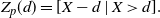 \begin{equation} Z_{p}(d)=[X-d\,|\,X>d].\end{equation}
This is a non-negative absolutely continuous random variable useful for describing instances in which the insurer covers the portion of the loss that exceeds d, provided the loss is greater than d. The PDF and SF of $Z_{p}(d)$
are given by
$Z_{p}(d)$
are given by
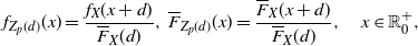 \begin{equation} f_{Z_{p}(d)}(x) = \frac{f_X(x+d)}{\overline{F}_X(d)}, \, \overline{F}_{Z_{p}(d)}(x) = \frac{\overline{F}_X(x+d)}{\overline{F}_X(d)}, \quad x\in \mathbb R^+_0,\end{equation}
where $\overline{F}_X(d)>0$
by assumption. Hence, recalling (33), we have
$\overline{F}_X(d)>0$
by assumption. Hence, recalling (33), we have ${\mathbb{E}}(Z_{p}(d)) = \mathsf{mrl}_X(d)$
. It follows that
${\mathbb{E}}(Z_{p}(d)) = \mathsf{mrl}_X(d)$
. It follows that
-
(i)
$X \le_{\mathrm{st}} Z_{p}(d)$
if and only if X is NWU, -
(ii)
$Z_{p}(d) \le_{\mathrm{st}} X$
if and only if X is NBU.


For case (i), recalling Eq. (33), we obtain
 \begin{align*}{\mathbb{E}}(Z_{p}(d)) - {\mathbb{E}} (X) = \mathsf{cmrl}_X(d),\end{align*}
so that, making use of Lemma 1 and Theorem 3, we have respectively
 \begin{align*}{\mathbb{E}} [g(Z_p(d))]-{\mathbb{E}}[g(X)]= {\mathbb{E}} [g'(Z)] \, \mathsf{cmrl}_X(d)\end{align*}
and
 \begin{align*}{\mathsf{Var}} [g(Z_p(d))]-{\mathsf{Var}}[g(X)]=2 \, \{{\mathbb{E}} [g'(Z) g(Z)] - {\mathbb{E}} [g'(Z)] {\mathbb{E}} [g(V)]\} \, \mathsf{cmrl}_X(d),\end{align*}
provided that $\mathsf{cmrl}(d)\neq 0$
. Here, the PDFs of Z and V, for
$\mathsf{cmrl}(d)\neq 0$
. Here, the PDFs of Z and V, for $x\in \mathbb R_0^+$
, are given respectively by
$x\in \mathbb R_0^+$
, are given respectively by
 \begin{align*}f_Z(x) = \frac{1}{\mathsf{cmrl}_X(d)} \, \left(\frac{\overline{F}_X(x+d)}{\overline{F}_X(d)} - \overline{F}_X(x) \right),\quad f_V(x) = \frac{1}{2} \, \frac{\overline{F}_X(x+d)}{\overline{F}_X(d)} + \frac{1}{2} \, \overline{F}_X(x).\end{align*}
We are now able to provide a result analogous to Theorem 9 under a different assumption.
Theorem 10. Let X be a non-negative absolutely continuous random variable, and let $Z_p(d)$
be defined as in (51). If X has DFR, then
$Z_p(d)$
be defined as in (51). If X has DFR, then
-
(i)
$X \leq_{\mathrm{hr}} Z_p(d)$
for all
$d\in \mathbb R^+$
; -
(ii)
$X \leq_{\mathrm{disp}} Z_p(d)$
for all
$d\in \mathbb R^+$
.


Proof. Recalling the definition of hazard rate given in the first part of Eq. (36) and the PDF of $Z_p(d)$
expressed in the first part of Eq. (52), we have
$Z_p(d)$
expressed in the first part of Eq. (52), we have
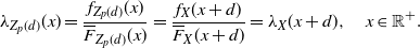 \begin{align*}\lambda_{Z_p(d)} (x)=\frac{f_{Z_p(d)}(x)}{\overline{F}_{Z_p(d)} (x)}=\frac{f_X(x+d)}{\overline{F}_X(x+d)}=\lambda_X (x+d),\quad x \in \mathbb R^+.\end{align*}
Hence, from the assumption that X has DFR it follows that $X \leq_{\mathrm{hr}} Z_p(d)$
for all
$X \leq_{\mathrm{hr}} Z_p(d)$
for all $d\in \mathbb R^+$
. Moreover, making use of Theorem 3.B.20, case (a), of [Reference Shaked and Shanthikumar28] one has
$d\in \mathbb R^+$
. Moreover, making use of Theorem 3.B.20, case (a), of [Reference Shaked and Shanthikumar28] one has $X \leq_{\mathrm{disp}} Z_p(d)$
. The proof is thus complete.
$X \leq_{\mathrm{disp}} Z_p(d)$
. The proof is thus complete.
The analysis of case (ii) proceeds in a similar way.
4.3. Per-loss residual loss
A situation in which the insurer pays zero for losses smaller than d can be described by using the per-loss residual loss $Z_l(d)$
. This is defined as
$Z_l(d)$
. This is defined as
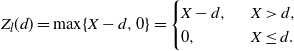 \begin{equation} Z_l(d)=\max\{X-d,0\}=\begin{cases} X-d, \ &\ X > d,\\ 0, \ &\ X \leq d.\end{cases}\end{equation}
Clearly, $Z_l(d)$
is a non-negative mixed random variable, composed of an absolutely continuous component over
$Z_l(d)$
is a non-negative mixed random variable, composed of an absolutely continuous component over $\mathbb R^+$
and a discrete one at 0. The SF of
$\mathbb R^+$
and a discrete one at 0. The SF of $Z_l(d)$
can be expressed as
$Z_l(d)$
can be expressed as
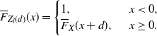 \begin{align*} \overline{F}_{Z_l(d)}(x) =\begin{cases} 1, \ &\ x < 0,\\ \overline{F}_X(x+d), \ &\ x \geq 0. \end{cases}\end{align*}
It thus follows that $Z_l(d) \leq_{\mathrm{st}} X$
. Consequently, for
$Z_l(d) \leq_{\mathrm{st}} X$
. Consequently, for $x\in \mathbb R^+_0$
, we have
$x\in \mathbb R^+_0$
, we have
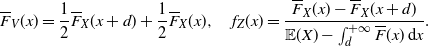 \begin{align*}\overline{F}_V (x) =\frac{1}{2} \overline{F}_{X}(x+d) + \frac{1}{2} \overline{F}_X (x),\quad f_Z (x) =\frac{\overline{F}_X (x)-\overline{F}_{X}(x+d)}{{\mathbb{E}}(X) - \int_{d}^{+\infty} \overline{F}(x) \, \mathrm{d}x}.\end{align*}
In the last term, ${\mathbb{E}}(X) - \int_{d}^{+\infty} \overline{F}(x) \, \mathrm{d}x = \int_{0}^{d} \overline{F}(x) \, \mathrm{d}x$
is of interest because it is associated with the loss elimination ratio (LER), an index with some interpretation in this topic (see, for example, Dimitriyadis and Oney [Reference Dimitriyadis and Öney14]). In particular, the LER of X evaluated at d is the equilibrium distribution given by
${\mathbb{E}}(X) - \int_{d}^{+\infty} \overline{F}(x) \, \mathrm{d}x = \int_{0}^{d} \overline{F}(x) \, \mathrm{d}x$
is of interest because it is associated with the loss elimination ratio (LER), an index with some interpretation in this topic (see, for example, Dimitriyadis and Oney [Reference Dimitriyadis and Öney14]). In particular, the LER of X evaluated at d is the equilibrium distribution given by
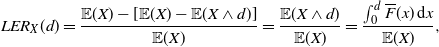 \begin{equation*} LER_{X}(d) = \frac{{\mathbb{E}}(X) - \left[{\mathbb{E}}(X) - {\mathbb{E}}(X \wedge d)\right]}{{\mathbb{E}}(X)} = \frac{{\mathbb{E}}(X \wedge d)}{{\mathbb{E}}(X)} = \frac{\int_{0}^d \overline{F}(x) \, \mathrm{d}x}{{\mathbb{E}}(X)},\end{equation*}
(where $\wedge$
means minimum) so that
$\wedge$
means minimum) so that $f_Z (x)$
can be rewritten as
$f_Z (x)$
can be rewritten as
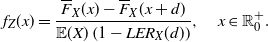 \begin{align*}f_Z (x) =\frac{\overline{F}_X (x)-\overline{F}_{X}(x+d)}{{\mathbb{E}}(X) \left(1-LER_X(d)\right)}, \quad x\in \mathbb R^+_0.\end{align*}
From Lemma 1 and Theorem 3, we have respectively
 \begin{align*}{\mathbb{E}} [g(X)]-{\mathbb{E}}[g(Z_l(d))]= {\mathbb{E}} [g'(Z)] \, {\mathbb{E}}(X) \left(1-LER_X(d)\right)\end{align*}
and
 \begin{align*}{\mathsf{Var}}[g(X)] - {\mathsf{Var}} [g(Z_l(d))]=2 \, \{{\mathbb{E}} [g'(Z) g(Z)] - {\mathbb{E}} [g'(Z)] {\mathbb{E}} [g(V)]\} \, {\mathbb{E}}(X) \left(1-LER_X(d)\right).\end{align*}
Our aim is now to compare the variance of two per-loss residual loss functions. Let X and Y be two non-negative absolutely continuous random variables such that $X \le_{\mathrm{st}} Y$
. By Eq. (53), their corresponding per-loss residual loss functions are given respectively by
$X \le_{\mathrm{st}} Y$
. By Eq. (53), their corresponding per-loss residual loss functions are given respectively by
 \begin{align*}Z_{X,l}(d)=\max\{X-d,0\}\equiv g(X),\quad Z_{Y,l}(d)=\max\{Y-d,0\}\equiv g(Y),\end{align*}
for $g(x) = (x - d)_+$
. We remark that
$g(x) = (x - d)_+$
. We remark that $Z_{X,l} (d)$
and
$Z_{X,l} (d)$
and $Z_{Y,l}(d)$
are mixed random variables with an atom at 0. Hence, using Theorem 3 and recalling Remark 5, we can obtain an expression for the difference between the variances of
$Z_{Y,l}(d)$
are mixed random variables with an atom at 0. Hence, using Theorem 3 and recalling Remark 5, we can obtain an expression for the difference between the variances of $Z_{X,l} (d)$
and
$Z_{X,l} (d)$
and $Z_{Y,l}(d)$
in terms of the difference between the expectations of X and Y, and in terms of the stop-loss functions of Z and V. Indeed, after few calculations we have
$Z_{Y,l}(d)$
in terms of the difference between the expectations of X and Y, and in terms of the stop-loss functions of Z and V. Indeed, after few calculations we have
 \begin{align*}{\mathsf{Var}}(Z_{Y,l}(d)) - {\mathsf{Var}}(Z_{X,l}(d))= 2 \, \left\{{\mathbb{E}}[(Z-d)_+] - \overline{F}_Z(d) \, {\mathbb{E}}[(V-d)_+] \right\}\, [{\mathbb{E}}(Y) - {\mathbb{E}}(X)],\end{align*}
where Z and V are the random variables given in (8) and (15), respectively.
5. The discrete case
In this section we aim to develop results analogous to those given in Section 2 with regard to random variables $Y\colon \Omega\to \mathbb N_0$
belonging to the set
$Y\colon \Omega\to \mathbb N_0$
belonging to the set ${\mathcal I}$
of integer-valued and non-negative random variables. Moreover, in this case the derivative is replaced by the difference operator.
${\mathcal I}$
of integer-valued and non-negative random variables. Moreover, in this case the derivative is replaced by the difference operator.
If the random variable $Y\in {\mathcal I}$
possesses finite non-zero mean
$Y\in {\mathcal I}$
possesses finite non-zero mean ${\mathbb{E}} (Y)$
, we can introduce the discrete equilibrium (residual lifetime) variable corresponding to Y, say
${\mathbb{E}} (Y)$
, we can introduce the discrete equilibrium (residual lifetime) variable corresponding to Y, say $Y_e^d$
, having probability function (see Section 7 of [Reference Di Crescenzo10], and Whitt [Reference Whitt31])
$Y_e^d$
, having probability function (see Section 7 of [Reference Di Crescenzo10], and Whitt [Reference Whitt31])
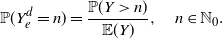 \begin{equation} \mathbb P (Y_e^d=n) = \frac{\mathbb P ( Y>n)}{ {\mathbb{E}} (Y)},\quad n\in \mathbb N_0.\end{equation}
In order to present the discrete versions of the probabilistic generalizations of Taylor’s theorem given in (3) and (6), let us now define the following operators:
 \begin{equation} \Delta g(n)=g(n+1)-g(n), \ Ag(n)=g(n+1)+g(n), \quad n \in \mathbb N_0,\end{equation}
for a general function $g\colon \mathbb N_0 \to \mathbb R$
.
$g\colon \mathbb N_0 \to \mathbb R$
.
Theorem 11. Let $Y\in {\mathcal I}$
possess finite non-zero mean
$Y\in {\mathcal I}$
possess finite non-zero mean ${\mathbb{E}} (Y)$
. If
${\mathbb{E}} (Y)$
. If $g\colon \mathbb N_0 \to \mathbb R$
is such that
$g\colon \mathbb N_0 \to \mathbb R$
is such that ${\mathbb{E}} [\Delta g(Y_e^d)]$
is finite, then
${\mathbb{E}} [\Delta g(Y_e^d)]$
is finite, then
 \begin{equation} {\mathbb{E}} [g(Y)] = g(0) + {\mathbb{E}} [\Delta g(Y_e^d)] \, {\mathbb{E}} (Y).\end{equation}
In addition, if ${\mathbb{E}} [\Delta g(Y_e^d) Ag(Y_e^d)]$
is finite, then
${\mathbb{E}} [\Delta g(Y_e^d) Ag(Y_e^d)]$
is finite, then
 \begin{equation*} {\mathbb{E}} [g^2(Y)] = g^2(0) + {\mathbb{E}} [\Delta g(Y_e^d) Ag(Y_e^d)] \, {\mathbb{E}} (Y).\end{equation*}
Proof. Making use of the first part of (55) we have
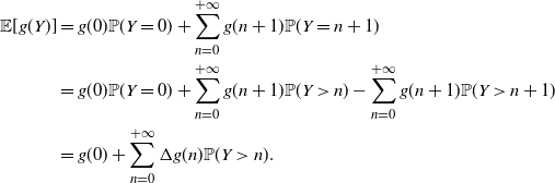 \begin{align*} \begin{split} {\mathbb{E}} [g(Y)] &= g(0) \mathbb P ( Y=0 ) + \sum_{n=0}^{+\infty} g(n+1) \mathbb P ( Y=n+1)\\ &= g(0) \mathbb P( Y=0 ) + \sum_{n=0}^{+\infty} g(n+1) \mathbb P ( Y>n) - \sum_{n=0}^{+\infty} g(n+1) \mathbb P ( Y>n+1 )\\ &= g(0) + \sum_{n=0}^{+\infty} \Delta g(n) \mathbb P ( Y>n).\end{split} \end{align*}
Hence, recalling (54), we obtain
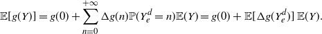 \begin{align*} {\mathbb{E}} [g(Y)] = g(0) + \sum_{n=0}^{+\infty} \Delta g(n) \mathbb P ( Y_e^d=n) {\mathbb{E}} (Y) = g(0) + {\mathbb{E}} [\Delta g(Y_e^d)] \, {\mathbb{E}} (Y).\end{align*}
Similarly, from (54) and (55) we have
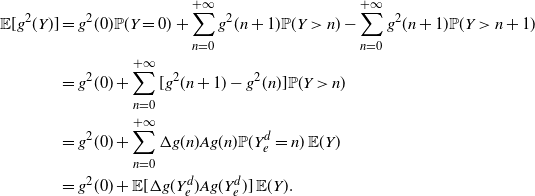 \begin{align*} \begin{split} {\mathbb{E}} [g^2(Y)] &= g^2(0) \mathbb P (Y=0) + \sum_{n=0}^{+\infty} g^2(n+1) \mathbb P (Y>n) - \sum_{n=0}^{+\infty} g^2(n+1) \mathbb P (Y>n+1)\\ &= g^2(0) + \sum_{n=0}^{+\infty} [g^2(n+1)-g^2(n)] \mathbb P (Y>n) \\ &= g^2(0) + \sum_{n=0}^{+\infty} \Delta g(n) Ag(n) \mathbb P (Y_e^d=n) \, {\mathbb{E}} (Y)\\ &= g^2(0) + {\mathbb{E}} [\Delta g(Y_e^d) Ag(Y_e^d)] \, {\mathbb{E}} (Y).\end{split} \end{align*}
The proof is thus complete.
Following Theorem 1, we are able to express ${\mathsf{Var}} [g(Y)]$
in terms of
${\mathsf{Var}} [g(Y)]$
in terms of ${\mathbb{E}} (Y)$
and of suitable expectations involving the operators in (55), as well as the random variables
${\mathbb{E}} (Y)$
and of suitable expectations involving the operators in (55), as well as the random variables $Y_e^d$
and
$Y_e^d$
and $\tilde{Y}$
, whose distributions are shown respectively in (54) and (5).
$\tilde{Y}$
, whose distributions are shown respectively in (54) and (5).
Theorem 12. Under the assumptions of Theorem 11, if $g\colon \mathbb N_0 \to \mathbb R$
is such that
$g\colon \mathbb N_0 \to \mathbb R$
is such that ${\mathbb{E}} \left [\Delta g(Y_e^d) Ag(Y_e^d)\right ]$
and
${\mathbb{E}} \left [\Delta g(Y_e^d) Ag(Y_e^d)\right ]$
and ${\mathbb{E}} [\Delta g(Y_e^d)]$
are finite, then
${\mathbb{E}} [\Delta g(Y_e^d)]$
are finite, then
 \begin{equation*} {\mathsf{Var}} [g(Y)] = \left \{ {\mathbb{E}} \left [\Delta g(Y_e^d) Ag(Y_e^d)\right ] - 2\,{\mathbb{E}} [\Delta g(Y_e^d)]\,{\mathbb{E}} [g(\tilde{Y})] \right \} {\mathbb{E}}(Y).\end{equation*}
Proof. We apply the results given in Theorem 11, so that
 \begin{align*}{\mathsf{Var}} [g(Y)] = g^2(0) + {\mathbb{E}} [\Delta g(Y_e^d) Ag(Y_e^d)] \, {\mathbb{E}} (Y) - (g(0) + {\mathbb{E}} [\Delta g(Y_e^d)] \, {\mathbb{E}} (Y))^2.\end{align*}
After some calculations we get
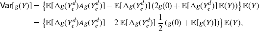 \begin{align*}\begin{split} {\mathsf{Var}} [g(Y)] =\ & \big \{ {\mathbb{E}} [\Delta g(Y_e^d) Ag(Y_e^d)] - {\mathbb{E}} [\Delta g(Y_e^d)] \, (2g(0) + {\mathbb{E}} [\Delta g(Y_e^d)] \, {\mathbb{E}} (Y)) \big \} \, {\mathbb{E}}(Y)\\ =\ & \big \{ {\mathbb{E}} [\Delta g(Y_e^d) Ag(Y_e^d)] - 2 \,{\mathbb{E}} [\Delta g(Y_e^d)] \, \frac{1}{2} \, (g(0) + {\mathbb{E}} [g(Y)] ) \big \} \, {\mathbb{E}}(Y),\end{split} \end{align*}
where the last equality is due to (56). Finally, the desired result follows when we recall Eq. (7).
To study the difference between the variance of two integer-valued random variables, we first recall the discrete version of PMVT given in [Reference Di Crescenzo10].
Lemma 2. If $X,Y\in {\mathcal I}$
are such that
$X,Y\in {\mathcal I}$
are such that $X \le_{\mathrm{st}} Y$
and
$X \le_{\mathrm{st}} Y$
and $ \mathbb{E}(X) < \mathbb{E}(Y) < +\infty$
, then there exists a
$ \mathbb{E}(X) < \mathbb{E}(Y) < +\infty$
, then there exists a $Z^d\in {\mathcal I}$
having probability function
$Z^d\in {\mathcal I}$
having probability function
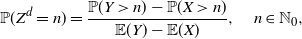 \begin{equation} \mathbb P(Z^d=n) = \frac{\mathbb P (Y>n) - \mathbb P (X>n)}{\mathbb{E}(Y) - \mathbb{E}(X)}, \quad n\in \mathbb{N}_0, \end{equation}
such that
 \begin{equation*} \mathbb{E}[g(Y)] - \mathbb{E}[g(X)] = \mathbb{E}[\Delta g(Z^d)] \, [\mathbb{E}(Y) - \mathbb{E}(X)], \end{equation*}
for $g\colon \mathbb N_0 \to \mathbb R$
being a function with
$g\colon \mathbb N_0 \to \mathbb R$
being a function with $\mathbb{E}[g(X)]$
and
$\mathbb{E}[g(X)]$
and $\mathbb{E}[g(Y)]$
finite.
$\mathbb{E}[g(Y)]$
finite.
The following results are the analogues of Theorem 3 and Corollary 2, respectively. The proofs are similar, and thus are omitted.
Theorem 13. Under the assumptions of Lemma 2, let $Z^d,V\in {\mathcal I}$
such that
$Z^d,V\in {\mathcal I}$
such that $Z^d$
has probability function (57) and V has CDF as defined in Eq. (15). If
$Z^d$
has probability function (57) and V has CDF as defined in Eq. (15). If $g\colon \mathbb N_0 \to \mathbb R$
is a function such that
$g\colon \mathbb N_0 \to \mathbb R$
is a function such that $\mathbb{E}[\Delta g(Z^d) Ag(Z^d)]$
and
$\mathbb{E}[\Delta g(Z^d) Ag(Z^d)]$
and $\mathbb{E}[\Delta g(Z^d)]$
are finite, then
$\mathbb{E}[\Delta g(Z^d)]$
are finite, then
 \begin{equation*} \mathsf{Var}[g(Y)] - \mathsf{Var}[g(X)] = \left \{ {\mathbb{E}} \left[\Delta g(Z^d) Ag(Z^d) \right] - 2 \,{\mathbb{E}} \left[\Delta g(Z^d) \right] {\mathbb{E}}[g(V)] \right \} [{\mathbb{E}} (Y) - {\mathbb{E}} (X)]. \end{equation*}
Remark 17. Similarly to the Remark 3, one has
-
(i)
${\mathbb{E}} \left [ A ( Z^d ) \right ]= 2\, \mathbb{E}(V)$
if and only if
$\mathsf{Var} (X) = \mathsf{Var} (Y)$
, -
(ii)
${\mathbb{E}} \left [ A ( Z^d ) \right ] > 2\,\mathbb{E}(V)$
if and only if
$\mathsf{Var} (X) < \mathsf{Var} (Y)$
.


Corollary 6. Under the assumptions of Theorem 13, if $\mathsf{Var} (X)\neq \mathsf{Var} (Y)$
then we have
$\mathsf{Var} (X)\neq \mathsf{Var} (Y)$
then we have
 \begin{equation*} \mathsf{Var}[g(Y)] - \mathsf{Var}[g(X)] = \Bigg \{\frac{ {\mathbb{E}} \left[\Delta g(Z^d)Ag(Z^d) \right] - 2\,{\mathbb{E}} \left[\Delta g(Z^d) \right]\,{\mathbb{E}}[g(V)]} { {\mathbb{E}} \left[ A( Z^d ) \right ] - 2\,{\mathbb{E}} (V)}\Bigg \} [\mathsf{Var} (Y) - \mathsf{Var} (X)].\end{equation*}
Analogously to Corollary 3, the following result holds:
Corollary 7. Under the assumption of Lemma 2, if $Y\in {\mathcal I}$
has finite non-zero mean
$Y\in {\mathcal I}$
has finite non-zero mean $\mathbb{E} (Y)$
, then
$\mathbb{E} (Y)$
, then
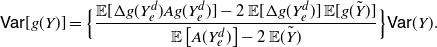 \begin{equation*} {\mathsf{Var}}[g(Y)] = \Big \{ \frac{ {\mathbb{E}} [\Delta g(Y_e^d)Ag(Y_e^d)] -2 \, {\mathbb{E}}[\Delta g(Y_e^d)]\,{\mathbb{E}}[g(\tilde{Y})]} { {\mathbb{E}} \left [ A(Y_e^d) \right ] -2 \,{\mathbb{E}} (\tilde{Y})}\Big \} {\mathsf{Var}} (Y). \end{equation*}
As done in Theorem 4, our aim is to express the variance of g(X) in terms of the variance of X in the present analysis. In the following, we will deal with the Gini mean semi-difference of X, which is a well-known coherent measure of variability defined as (cf. Hu and Chen [Reference Hu and Chen18], for instance)
 \begin{equation} \mathsf{Gini}(X) \;:\!=\;\frac{1}{2}\, \mathsf{GMD}(X),\end{equation}
where $\mathsf{GMD}(X)$
is defined in (28).
$\mathsf{GMD}(X)$
is defined in (28).
Theorem 14. Let $X\in {\mathcal I}$
be such that
$X\in {\mathcal I}$
be such that ${\mathsf{Var}} (X)$
is finite and non-zero, and let
${\mathsf{Var}} (X)$
is finite and non-zero, and let $X_G\in {\mathcal I}$
have probability function
$X_G\in {\mathcal I}$
have probability function
 \begin{equation} \mathbb{P} (X_G=n) = \frac{ \mathbb P (X \leq n) \,\mathbb P (X >n)}{\mathsf{Gini}(X)}, \quad n \in \mathbb N_0.\end{equation}
Let $(X_1^*,X_2^*)$
be an integer-valued non-negative random vector having joint probability function
$(X_1^*,X_2^*)$
be an integer-valued non-negative random vector having joint probability function
 \begin{equation} p^* (n_1,n_2)\;:\!=\; \mathbb{P} (X_1^*=n_1,X_2^*=n_2)= \frac{2 \, \mathbb P (X \leq n_1) \,\mathbb P (X > n_2)}{{\mathsf{Var}} (X) - \mathsf{Gini}(X)} \, \mathbf{1}_{\{n_1 < n_2\}},\quad n_1,n_2 \in \mathbb N_0.\end{equation}
If $g\colon \mathbb N_0 \to \mathbb R$
is a function such that
$g\colon \mathbb N_0 \to \mathbb R$
is a function such that ${\mathbb{E}}\left[\Delta g^2 (X_G)\right]$
and
${\mathbb{E}}\left[\Delta g^2 (X_G)\right]$
and ${\mathbb{E}} [ \Delta g(X_1^*) \Delta g(X_2^*)]$
are finite, then
${\mathbb{E}} [ \Delta g(X_1^*) \Delta g(X_2^*)]$
are finite, then
 \begin{equation} {\mathsf{Var}} [g(X)] = \mathsf{Gini}(X) \,{\mathbb{E}}\left[\Delta g^2 (X_G)\right] +\left[ {\mathsf{Var}} (X)-\mathsf{Gini}(X)\right] \, {\mathbb{E}} [ \Delta g(X_1^*) \, \Delta g(X_2^*)].\end{equation}
Proof. Following the probabilistic generalization of Taylor’s theorem (cf. [Reference Massey and Whitt21]), we have
 \begin{align*} {\mathsf{Var}} [g(X)] = {\mathsf{Var}} [g(X) - g(0)]= {\mathsf{Var}} \left [ \sum_{n=0}^{X-1} \Delta g(n) \right ] = {\mathsf{Var}} \left [ \sum_{n=0}^{+\infty} \mathbf{1}_{\{X>n\}} \Delta g(n) \right ].\end{align*}
The decomposition of the variance thus yields
 \begin{equation*}\begin{split} {\mathsf{Var}} [g(X)]& = \sum_{n=0}^{+\infty} {\mathsf{Var}} \left [ \mathbf{1}_{\{X>n\}} \right ] \Delta g^2 (n)\\ &\quad+ 2 \sum_{n_1=0}^{+\infty} \sum_{n_2=n_1+1}^{+\infty} \left( {\mathbb{E}} \left[ \mathbf{1}_{\{X>n_1\}} \mathbf{1}_{\{X>n_2\}} \right] - {\mathbb{E}} \left[ \mathbf{1}_{\{X>n_1\}} \right] {\mathbb{E}} \left[ \mathbf{1}_{\{X>n_2\}} \right] \right) \Delta g(n_1) \Delta g(n_2) \\ &= \sum_{n=0}^{+\infty} \mathbb P (X \leq n) \mathbb P (X>n) \Delta g^2 (n) \\ &\quad+ 2 \sum_{n_1=0}^{+\infty} \sum_{n_2=n_1+1}^{+\infty} \mathbb P (X \leq n_1) \mathbb P (X>n_2) \Delta g(n_1) \Delta g(n_2).\end{split}\end{equation*}
Making use of (59) and (60), we have
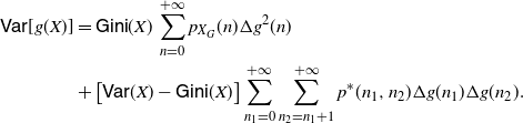 \begin{equation*}\begin{split} {\mathsf{Var}} [g(X)] & = \mathsf{Gini}(X) \, \sum_{n=0}^{+\infty} p_{X_G} (n) \Delta g^2 (n) \\ & + \left[{\mathsf{Var}} (X) - \mathsf{Gini}(X) \right]\sum_{n_1=0}^{+\infty} \sum_{n_2=n_1+1}^{+\infty} p^* (n_1,n_2) \Delta g(n_1) \Delta g(n_2).\end{split}\end{equation*}
Then Eq. (61) immediately follows.
Remark 18. Under the assumptions of Theorem 14, we have ${\mathsf{Var}} (X)> \mathsf{Gini}(X)$
. Indeed, making use of Fubini’s theorem and equation (58), one has
${\mathsf{Var}} (X)> \mathsf{Gini}(X)$
. Indeed, making use of Fubini’s theorem and equation (58), one has
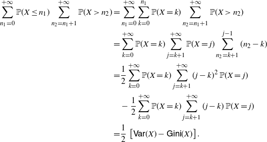 \begin{align*}\begin{split} \sum_{n_1=0}^{+\infty} \mathbb P (X \leq n_1) \sum_{n_2=n_1+1}^{+\infty} \mathbb P (X > n_2) =& \sum_{n_1=0}^{+\infty} \sum_{k=0}^{n_1} \mathbb{P} (X = k) \sum_{n_2=n_1+1}^{+\infty} \mathbb P (X > n_2) \\ =& \sum_{k=0}^{+\infty} \mathbb{P} (X = k) \sum_{j=k+1}^{+\infty} \mathbb P (X =j) \sum_{n_2=k+1}^{j-1} (n_2-k) \\ =& \frac{1}{2} \sum_{k=0}^{+\infty} \mathbb{P} (X = k) \sum_{j=k+1}^{+\infty} (j-k)^2 \,\mathbb P (X =j) \\ &- \frac{1}{2} \sum_{k=0}^{+\infty} \mathbb{P} (X = k) \sum_{j=k+1}^{+\infty} (j-k)\, \mathbb P (X =j) \\ =& \frac{1}{2}\, \left[ {\mathsf{Var}} (X)- \mathsf{Gini}(X)\right].\end{split}\end{align*}
Hence, by virtue of (60), $(X_1^*,X_2^*)$
is an honest discrete random vector. Similarly, we have
$(X_1^*,X_2^*)$
is an honest discrete random vector. Similarly, we have
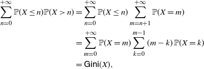 \begin{align*}\begin{split} \sum_{n=0}^{+\infty} \mathbb P (X \leq n) \mathbb P (X>n) &= \sum_{n=0}^{+\infty} \mathbb P (X \leq n) \sum_{m=n+1}^{+\infty} \mathbb P (X=m) \\ &= \sum_{m=0}^{+\infty} \mathbb P (X=m) \sum_{k=0}^{m-1} (m-k) \,\mathbb P (X=k) \\ &= \mathsf{Gini}(X),\end{split}\end{align*}
so that $X_G$
is an honest discrete random variable due to (59).
$X_G$
is an honest discrete random variable due to (59).
Table 3 shows some examples of probability functions $p^*(n_1,n_2)$
obtained for suitable choices of discrete random variables. In case (iv) one has
$p^*(n_1,n_2)$
obtained for suitable choices of discrete random variables. In case (iv) one has $c={\mathsf{Var}} (X) - \mathsf{Gini}(X)=\frac{\pi ^3}{3} \left ( 1+ \frac{\pi ^3}{319} \right ) - \zeta (3) \left[2 + \zeta (3)\right]$
, where
$c={\mathsf{Var}} (X) - \mathsf{Gini}(X)=\frac{\pi ^3}{3} \left ( 1+ \frac{\pi ^3}{319} \right ) - \zeta (3) \left[2 + \zeta (3)\right]$
, where $\zeta $
denotes the Euler–Riemann zeta function. Moreover, in case (v),
$\zeta $
denotes the Euler–Riemann zeta function. Moreover, in case (v), $H_{n}= \sum_{k=0}^{n} \frac{1}{k}$
is the nth harmonic number.
$H_{n}= \sum_{k=0}^{n} \frac{1}{k}$
is the nth harmonic number.
Analogously to point (i) of Corollary 4 we can now provide the marginal distributions of $(X_1^*,X_2^*)$
.
$(X_1^*,X_2^*)$
.
Corollary 8. Under the assumptions of Theorem 14, the probability functions of $X_1^*$
and
$X_1^*$
and $X_2^*$
are respectively given by
$X_2^*$
are respectively given by
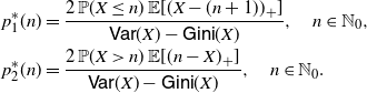 \begin{equation} \begin{split} p_1^* (n) &= \frac{2 \, \mathbb P (X \leq n) \,{\mathbb{E}} [(X-(n+1))_{+}]}{{\mathsf{Var}} (X) - \mathsf{Gini}(X)}, \quad n \in \mathbb N_0,\\ p_2^* (n ) &= \frac{2 \, \mathbb P (X >n) \,{\mathbb{E}} [(n-X)_{+}]}{{\mathsf{Var}} (X) - \mathsf{Gini}(X)}, \quad n \in \mathbb N_0. \end{split} \end{equation}
Table 4 shows the probability functions of $X_1^*$
and
$X_1^*$
and $X_2^*$
provided in Eq. (62), where c and
$X_2^*$
provided in Eq. (62), where c and $H_{n}$
are the same quantities as in Table 3. Furthermore, in case (iv),
$H_{n}$
are the same quantities as in Table 3. Furthermore, in case (iv), $\Psi (n) = \frac{{\mathrm{d}}}{{\mathrm{d}} n} \ln \Gamma (n) = \frac{1}{\Gamma (n)} \frac{{\mathrm{d}}}{{\mathrm{d}} n} \Gamma (n)$
is the digamma function. Finally, Table 5 shows the probability function of
$\Psi (n) = \frac{{\mathrm{d}}}{{\mathrm{d}} n} \ln \Gamma (n) = \frac{1}{\Gamma (n)} \frac{{\mathrm{d}}}{{\mathrm{d}} n} \Gamma (n)$
is the digamma function. Finally, Table 5 shows the probability function of $X_G$
obtained for the random variables considered in Table 3.
$X_G$
obtained for the random variables considered in Table 3.
Table 3. Examples of joint probabilities $p^*(n_1,n_2)$
for some choices of discrete random variables.
$p^*(n_1,n_2)$
for some choices of discrete random variables.
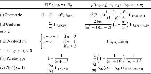
Table 4. Probability functions $p_1^*(n)$
and
$p_1^*(n)$
and $p_2^*(n)$
for the examples of Table 3.
$p_2^*(n)$
for the examples of Table 3.
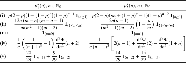
Table 5. Probability function of $X_G$
for the examples of Table 3.
$X_G$
for the examples of Table 3.
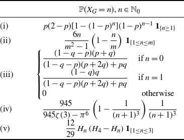
Note that Remark 10 holds also for the marginal distributions of $X_1^*$
and
$X_1^*$
and $X_2^*$
given in (62), by considering: (i) the first- and second-order discrete equilibrium distributions of X, denoted respectively by
$X_2^*$
given in (62), by considering: (i) the first- and second-order discrete equilibrium distributions of X, denoted respectively by $X_e^d$
and
$X_e^d$
and $X_{e_2}^d$
; and (ii) the random variable
$X_{e_2}^d$
; and (ii) the random variable $X_e^L$
having probability mass function
$X_e^L$
having probability mass function $\mathbb{P} (X_e^L=n)=(n+1) \, \mathbb{P}(X_e^d=n)/{\mathbb{E}} (X_e^d)$
.
$\mathbb{P} (X_e^L=n)=(n+1) \, \mathbb{P}(X_e^d=n)/{\mathbb{E}} (X_e^d)$
.
Moreover, by analogy with Remark 12, by recalling (35) and (62), the random variables $X_1^*$
and
$X_1^*$
and $X_2^*$
can be seen as discrete weighted versions of the discrete equilibrium variable
$X_2^*$
can be seen as discrete weighted versions of the discrete equilibrium variable $X_e^d$
, where the weights depend on the functions
$X_e^d$
, where the weights depend on the functions
 \begin{align*}\mathsf{mrl}^d(n) =\displaystyle\frac{1}{\mathbb{P}(X>n)} \sum_{x=n}^{+\infty} \mathbb{P}(X>x), \mathsf{mit}^d(n) = \displaystyle \frac{1}{\mathbb{P}(X\leq n)} \sum_{x=0}^{n} \mathbb{P}(X\leq x),\quad n \in \mathbb N_0.\end{align*}
Similarly to (33) and (34), $\mathsf{mrl}^d(n)$
and
$\mathsf{mrl}^d(n)$
and $\mathsf{mit}^d(n)$
constitute respectively the discrete mean residual lifetime and the discrete mean inactivity time of X (cf. Sections 2.2.3 and 2.2.7 of Unnikrishnan Nair et al. [Reference Unnikrishnan Nair, Sankaran and Balakrishnan29]).
$\mathsf{mit}^d(n)$
constitute respectively the discrete mean residual lifetime and the discrete mean inactivity time of X (cf. Sections 2.2.3 and 2.2.7 of Unnikrishnan Nair et al. [Reference Unnikrishnan Nair, Sankaran and Balakrishnan29]).
Remark 19. Under the assumptions of Theorem 14, if X has finite discrete mean residual lifetime and discrete mean inactivity time, then
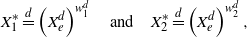 \begin{align*}X_1^* \stackrel{d}{=} \left ( X_e^{d} \right )^{w_1^d} \quad \text{and} \quad X_2^* \stackrel{d}{=} \left ( X_e^{d} \right )^{w_2^d},\end{align*}
where $w_1^d(n)= \mathbb{P}(X \leq n) \,(\mathsf{mrl}^d(n)-1)$
and
$w_1^d(n)= \mathbb{P}(X \leq n) \,(\mathsf{mrl}^d(n)-1)$
and $w_2^d(n)= \mathbb{P}(X \leq n)\,\mathsf{mit}^d(n)$
, for all
$w_2^d(n)= \mathbb{P}(X \leq n)\,\mathsf{mit}^d(n)$
, for all $n\in \mathbb N_0^+$
.
$n\in \mathbb N_0^+$
.
6. Concluding remarks
This paper has analysed the variances of transformed random variables and their differences for stochastically ordered random variables, thanks to the use of PMVT. We investigated the connections with the equilibrium operator and suitably related random variables. The analysis also allowed us to introduce useful joint distributions connected to the mean residual lifetime and the mean inactivity time, as well as some applications to the additive hazards model and to notions of interest in actuarial science.
Possible developments of the present analysis may focus on customary extensions in which the role of the equilibrium distribution is played by iterates of the equilibrium distribution itself, which has been usefully exploited in contexts related to the probabilistic generalization of Taylor’s theorem (cf. Massey and Whitt [Reference Massey and Whitt21] and Lin [Reference Lin20]) and for the construction of sequences of stochastic orders (see Fagiuoli and Pellerey [Reference Fagiuoli and Pellerey15]). Moreover, a possible future line of research includes the development of the fractional extension of the given results, on the basis of the fractional probabilistic analogues studied in Di Crescenzo and Meoli [Reference Di Crescenzo and Meoli11].
Acknowledgements
A. Di Crescenzo and G. Pisano are members of the research group GNCS of the Istituto Nazionale di Alta Matematica (INdAM).
Funding information
The authors acknowledge support received from the “European Union – Next Generation EU” through MUR-PRIN 2022, project 2022XZSAFN “Anomalous Phenomena on Regular and Irregular Domains: Approximating Complexity for the Applied Sciences,” and MUR-PRIN 2022 PNRR, project P2022XSF5H “Stochastic Models in Biomathematics and Applications.”
Competing interests
There were no competing interests to declare arising during the preparation or publication process of this article.


 Open access