1. Introduction
Consider the problem of stochastic simulation from a target distribution,
![]() $\pi(x),$
on a d-dimensional state space
$\pi(x),$
on a d-dimensional state space
![]() $\mathcal{X}$
where
$\mathcal{X}$
where
![]() $\pi({\cdot})$
is known up to a scaling constant. The gold standard methodology for this problem uses Markov chain Monte Carlo (MCMC). However, these methods often perform poorly in the context of multimodality.
$\pi({\cdot})$
is known up to a scaling constant. The gold standard methodology for this problem uses Markov chain Monte Carlo (MCMC). However, these methods often perform poorly in the context of multimodality.
Most MCMC algorithms use localised proposal mechanisms, tuned towards local approximate optimality, e.g. [Reference Roberts and Rosenthal31] and [Reference Roberts, Gelman and Gilks35]. Indeed, many MCMC algorithms incorporate local gradient information in the proposal mechanisms, typically attracting the chain back towards the centre of the mode. This can exacerbate the difficulties of moving between modes [Reference Mangoubi, Pillai and Smith17].
Popular methods used to overcome these issues include simulated tempering [Reference Marinari and Parisi18] and the population-based version, parallel tempering [Reference Geyer8], [Reference Geyer and Thompson9]. These methods use state space augmentation to allow Markov chains to explore target distributions proportional to
![]() $\pi ^{\beta } (x)$
for
$\pi ^{\beta } (x)$
for
![]() $\beta$
typically in the range (0,1]. For simulated tempering, this is done by introducing an auxiliary inverse temperature variable,
$\beta$
typically in the range (0,1]. For simulated tempering, this is done by introducing an auxiliary inverse temperature variable,
![]() $\beta $
, and running a
$\beta $
, and running a
![]() $(d+1)$
-dimensional Markov chain on
$(d+1)$
-dimensional Markov chain on
![]() $\mathcal{X}\times \Delta$
, where
$\mathcal{X}\times \Delta$
, where
![]() $\Delta $
consists of a discrete collection of possible inverse temperatures including 1. For the more practically applicable parallel tempering approach, a Markov chain is run on a
$\Delta $
consists of a discrete collection of possible inverse temperatures including 1. For the more practically applicable parallel tempering approach, a Markov chain is run on a
![]() $(|\Delta|\times
d)$
-dimensional state space,
$(|\Delta|\times
d)$
-dimensional state space,
![]() $\smash{\mathcal{X}^{|\Delta|}}$
, where
$\smash{\mathcal{X}^{|\Delta|}}$
, where
![]() $|\Delta|$
denotes the cardinality of the set
$|\Delta|$
denotes the cardinality of the set
![]() $\Delta$
.
$\Delta$
.
Within this paper we will concentrate on parallel tempering as it obviates the need to approximate certain normalisation constants to work effectively. While parallel tempering has been highly successful, for example, see [Reference Carter and White5], [Reference Mohamed20], [Reference Xie, Zhou and Jiang49], etc., its efficiency declines as a function of d, at least linearly and often much worse [Reference Atchadé, Roberts and Rosenthal1], [Reference Woodard, Schmidler and Huber48]. This is caused by the need to set inter-inverse temperature spacings in
![]() $\Delta $
extremely small to make swaps between temperatures feasible.
$\Delta $
extremely small to make swaps between temperatures feasible.
In this paper we introduce and analyse the QuanTA algorithm which facilitates inter-temperature swaps by proposing moves which attempt to adjust within-mode variation appropriately for the proposed new temperature. This leads to improved temperature mixing, which in turn leads to vastly improved inter-modal mixing. Its typical improvement is demonstrated in Figure 1 with a five-mode target distribution. The construction of QuanTA resonates with the noncentering MCMC methodology described, for example, in [Reference Brooks, Giudici and Roberts4], [Reference Hastie12], [Reference Papaspiliopoulos and Roberts25], and [Reference Papaspiliopoulos, Roberts and Sköld26].
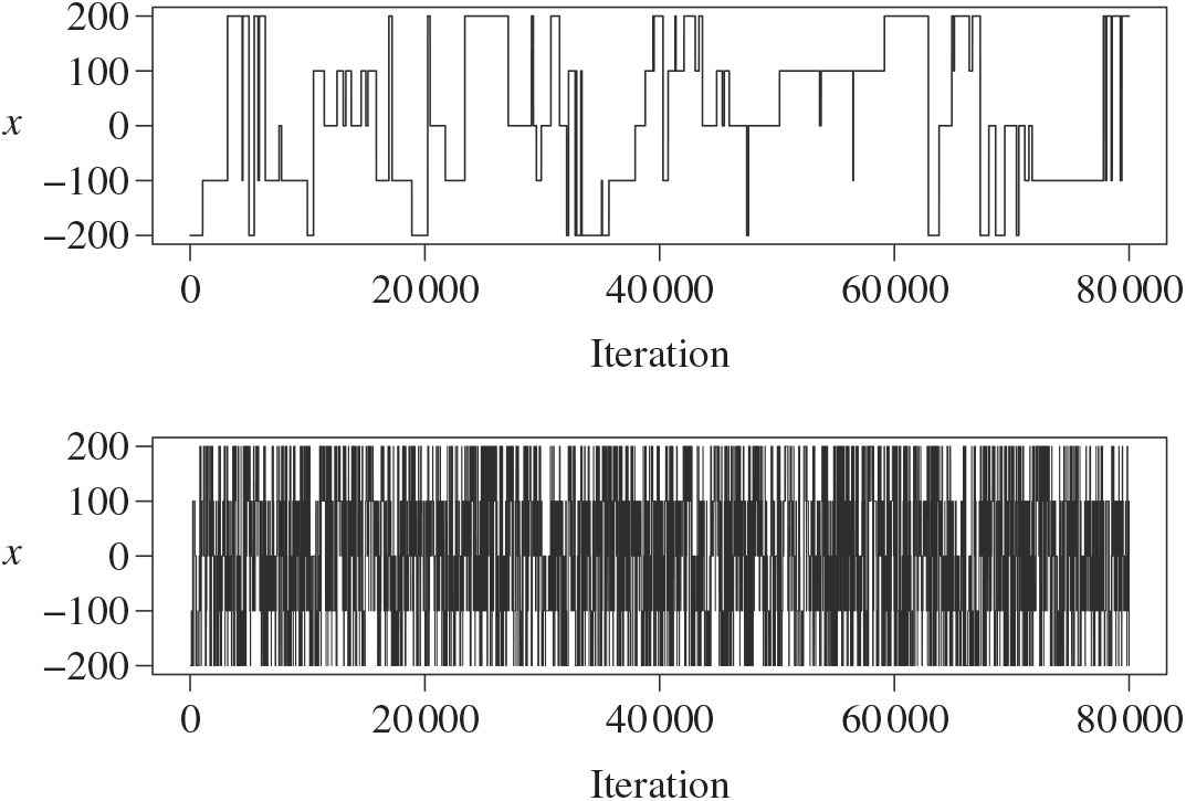
Figure 1: Trace plots of the target state chains for representative runs of the parallel tempering (top) and QuanTA schemes (bottom).
Supporting theory is developed to guide setup and analyse the utility of the novel QuanTA scheme. There are two key theoretical results. The first, Theorem 1, establishes that there is an optimal temperature schedule setup for QuanTA, concluding that in general the dimensionality scaling of the distance between consecutive inverse temperature spacings should be
![]() $\mathcal{O}(d^{-1/2})$
. Further to this it suggests that optimising the expected squared jumping distance between any two consecutive temperature levels induces a temperature swap move acceptance rate of 0.234, giving a useful metric for a practitioner to optimally tune QuanTA. The second key theoretical contribution, Theorem 2, of this paper shows that, under mild regularity conditions, the optimal temperature spacings of QuanTA are more ambitiously spaced than for the standard parallel tempering algorithm for cold (i.e. large) values of the inverse temperatures. The significance of this result is that QuanTA can give accelerated mixing through the cooler parts of the temperature schedule by allowing more ambitious temperature spacings.
$\mathcal{O}(d^{-1/2})$
. Further to this it suggests that optimising the expected squared jumping distance between any two consecutive temperature levels induces a temperature swap move acceptance rate of 0.234, giving a useful metric for a practitioner to optimally tune QuanTA. The second key theoretical contribution, Theorem 2, of this paper shows that, under mild regularity conditions, the optimal temperature spacings of QuanTA are more ambitiously spaced than for the standard parallel tempering algorithm for cold (i.e. large) values of the inverse temperatures. The significance of this result is that QuanTA can give accelerated mixing through the cooler parts of the temperature schedule by allowing more ambitious temperature spacings.
This paper is structured into six core sections. In Sections 2 we review the parallel tempering algorithm and some of the relevant existing literature. Section 3 motivates the main idea behind the novel QuanTA scheme, which is then presented in Section 4. QuanTA utilises a population MCMC approach that requires a clustering scheme; discussion for this is found in Section 5. Section 6 contains the core theoretical contributions mentioned above. Simulation studies are detailed in Section 7 along with a discussion of the computational complexity of QuanTA.
2. The parallel tempering algorithm
There is an array of methodology available to overcome the issues of multimodality using MCMC or closely related sequential Monte Carlo (SMC) techniques, e.g. [Reference Geyer8], [Reference Kou, Zhou and Wong16], [Reference Marinari and Parisi18], [Reference Neal21], [Reference Nemeth, Lindsten, Filippone and Hensman23], [Reference Paulin, Jasra and Thiery28], [Reference Schweizer37], and [Reference Wang and Swendsen46]. The majority of these methods use state space augmentation approaches. Auxiliary distributions that allow a Markov chain to explore the entirety of the state space are targeted and their mixing information is then passed on to aid inter-modal mixing in the desired target. A convenient approach for the augmentation methods is to use power-tempered target distributions i.e. the target distribution at inverse temperature level,
![]() $\beta$
, for
$\beta$
, for
![]() $\beta \in (0,1]$
is defined as
$\beta \in (0,1]$
is defined as
Such targets are the most common choice of auxiliary target when augmenting the state space for use in the popular simulated tempering (ST) and parallel tempering (PT) algorithms introduced in [Reference Marinari and Parisi18] and [Reference Geyer8]. For each algorithm, one needs to choose a sequence of
![]() $n+1$
‘inverse temperatures’,
$n+1$
‘inverse temperatures’,
![]() $\Delta=\{\beta_0,\ldots,\beta_n\}$
, where
$\Delta=\{\beta_0,\ldots,\beta_n\}$
, where
![]() $0 \leq
\beta_n<\beta_{n-1}<\cdots <\beta_1<\beta_0=1$
with the specification that a Markov chain sampling from the target distribution
$0 \leq
\beta_n<\beta_{n-1}<\cdots <\beta_1<\beta_0=1$
with the specification that a Markov chain sampling from the target distribution
![]() $\pi_{\beta_n}(x)$
can mix well across the entire state space.
$\pi_{\beta_n}(x)$
can mix well across the entire state space.
The PT algorithm runs a Markov chain on the augmented state space,
![]() $\mathcal{X}^{(n+1)}$
, targeting an invariant distribution given by
$\mathcal{X}^{(n+1)}$
, targeting an invariant distribution given by
From an initialisation point for the chain, the PT algorithm alternates between two types of Markovian move: within temperature Markov chain moves that use standard localised MCMC schemes to update each of the
![]() $x_i$
whilst preserving marginal invariance; temperature swap moves that propose to swap the chain locations between a pair of adjacent temperature components. It is these swap moves that will allow mixing information from the hot, rapidly mixing temperature level to be passed to aid mixing at the cold target state.
$x_i$
whilst preserving marginal invariance; temperature swap moves that propose to swap the chain locations between a pair of adjacent temperature components. It is these swap moves that will allow mixing information from the hot, rapidly mixing temperature level to be passed to aid mixing at the cold target state.
To perform the swap move, a pair of temperatures is chosen uniformly from the set of all adjacent pairs, call this pair
![]() $x_i$
and
$x_i$
and
![]() $x_{i+1}$
at inverse temperatures
$x_{i+1}$
at inverse temperatures
![]() $\beta_{x_i}$
and
$\beta_{x_i}$
and
![]() $\beta_{x_{i+1}},$
respectively. The proposal is then
$\beta_{x_{i+1}},$
respectively. The proposal is then
To preserve detailed balance and therefore invariance to
![]() $\pi_n({\cdot})$
, the swap move is accepted with probability
$\pi_n({\cdot})$
, the swap move is accepted with probability
It is the combination of the suitably specified within temperature moves and temperature swap moves that ensures ergodicity of the Markov chain to the target distribution,
![]() $\pi_n({\cdot})$
. Note that the within temperature moves certainly influence the performance of the algorithm [Reference Ge, Lee and Risteski7]; however, the focus of the work in this article will be on designing a novel approach for the temperature swap move.
$\pi_n({\cdot})$
. Note that the within temperature moves certainly influence the performance of the algorithm [Reference Ge, Lee and Risteski7]; however, the focus of the work in this article will be on designing a novel approach for the temperature swap move.
The novel work presented in this paper focuses on the setting where the d-dimensional state space is given by
![]() $\mathbb{R}^d$
and the target,
$\mathbb{R}^d$
and the target,
![]() $\pi({\cdot})$
, is the associated probability density function. Thus, herein take
$\pi({\cdot})$
, is the associated probability density function. Thus, herein take
![]() $\mathcal{X} = \mathbb{R}^d,$
but note that natural generalisations to other state spaces and settings are possible.
$\mathcal{X} = \mathbb{R}^d,$
but note that natural generalisations to other state spaces and settings are possible.
3. Modal rescaling transformation
3.1 A motivating transformation move
Consider a PT algorithm that has two components
![]() $x_1$
and
$x_1$
and
![]() $x_2$
running at the neighbouring inverse temperature levels
$x_2$
running at the neighbouring inverse temperature levels
![]() $\beta$
and
$\beta$
and
![]() $\beta^{'}$
. Suppose that a temperature swap move is proposed between the two chains at the two temperature levels. Due to the dependence between the location in the state space and the temperature level,
$\beta^{'}$
. Suppose that a temperature swap move is proposed between the two chains at the two temperature levels. Due to the dependence between the location in the state space and the temperature level,
![]() $\beta$
and
$\beta$
and
![]() $\beta^{'}$
need to be close to each other to avoid the move having negligible acceptance probability. Intuitively, the problem is that the proposal from the hotter chain is likely to be an ‘unrepresentative’ location at the colder temperature, and vice versa.
$\beta^{'}$
need to be close to each other to avoid the move having negligible acceptance probability. Intuitively, the problem is that the proposal from the hotter chain is likely to be an ‘unrepresentative’ location at the colder temperature, and vice versa.
So there is clearly a significant dependence between the temperature value and the location of the chain in the state space, thus explaining why temperature swap moves between arbitrarily largely spaced temperatures are generally rejected. This issue is typically exacerbated when the dimensionality grows.
Consider, for motivational purposes, a simple one-dimensional setting where the state space is given by
![]() $\mathbb{R}$
and the target density is given by
$\mathbb{R}$
and the target density is given by
![]() $\pi({\cdot})$
. For notational convenience, letting
$\pi({\cdot})$
. For notational convenience, letting
![]() $j\,{=}\,i\,{+}\,1$
, suppose that a temperature swap move has been proposed between adjacent levels
$j\,{=}\,i\,{+}\,1$
, suppose that a temperature swap move has been proposed between adjacent levels
![]() $\beta_i$
and
$\beta_i$
and
![]() $\beta_j$
with marginal component values
$\beta_j$
with marginal component values
![]() $x_i$
and
$x_i$
and
![]() $x_j,$
respectively.
$x_j,$
respectively.
Suppose that an oracle has provided a function,
![]() $t_{ij}\colon
\mathbb{R}\!\rightarrow\! \mathbb{R}$
, that is bijective, with
$t_{ij}\colon
\mathbb{R}\!\rightarrow\! \mathbb{R}$
, that is bijective, with
![]() $t_{ji}(t_{ij}(x))\,{=}\,x$
, and differentiable and preserves the cumulative distribution function (CDF) between the two temperature levels such that
$t_{ji}(t_{ij}(x))\,{=}\,x$
, and differentiable and preserves the cumulative distribution function (CDF) between the two temperature levels such that
where
![]() $F_{\beta} ( \cdot)$
denotes the CDF of
$F_{\beta} ( \cdot)$
denotes the CDF of
![]() $\pi^\beta({\cdot})$
.
$\pi^\beta({\cdot})$
.
Suppose that rather than the standard temperature swap move proposal in (2), the following is instead proposed:
To preserve detailed balance, this is accepted with an acceptance ratio similar to reversible-jump MCMC [Reference Green10] to account for the deterministic transformation:
By differentiating (3) with respect to x and rearranging
Using the result in (5), and noting the cancellation of normalising constants in (4), we can see that (4) evaluates to 1 and, hence, such a swap would always be accepted. Essentially, the transformation
![]() $t_{ij}({\cdot})$
has made the acceptance probability of a temperature swap move independent of the locations of
$t_{ij}({\cdot})$
has made the acceptance probability of a temperature swap move independent of the locations of
![]() $x_i$
and
$x_i$
and
![]() $x_j$
in the state space.
$x_j$
in the state space.
In practice, a CDF-preserving transformation
![]() $t_{ij}({\cdot})$
will not generally be available. Consider a simplified setting when the target is now a d-dimensional Gaussian, i.e.
$t_{ij}({\cdot})$
will not generally be available. Consider a simplified setting when the target is now a d-dimensional Gaussian, i.e.
![]() $\pi\sim N(\mu,\Sigma)$
, and so the tempered target at inverse temperature
$\pi\sim N(\mu,\Sigma)$
, and so the tempered target at inverse temperature
![]() $\beta$
is given by
$\beta$
is given by
![]() $\pi^\beta \sim N(\mu,\Sigma /\beta)$
. Defining a d-dimensional transformation by
$\pi^\beta \sim N(\mu,\Sigma /\beta)$
. Defining a d-dimensional transformation by
a simple calculation shows that in this setting such a transformation, which only requires knowledge of the mode location, permits swap moves to always be accepted independently of the dimensionality and magnitude of the inverse temperature spacings.
In a broad class of applications it is not unreasonable to make a Gaussian approximation to posterior modes [Reference Rue, Martino and Chopin36]. Indeed, this is the motivation for the similar transformation derived in [Reference Hastie12] for use in a reversible-jump MCMC framework.
Beyond a single-dimensional setting a quantile is typically nonunique since multiple locations in the state space produce the same CDF evaluation. However, the transformation in (6), motivated via Gaussianity, is bijective and can be seen as a way of uniquely pairing two quantiles at different temperature levels allowing for ‘quantile uniqueness’ and, therefore, reversibility of the transformation. It is from this that QuanTA gets its name.
3.2 Transformation-aided move in a PT framework
In a multimodal setting a single Gaussian approximation to the posterior will be poor. However, it is often reasonable that the local modes may be individually approximated as Gaussian. In this paper we explore the use of the transformation in (6) applied to the local mode with the aim being to accelerate the mixing through the temperature schedule of a PT algorithm.
Now that the transformations are localised to modes we need careful specification of the transformation function. Suppose that there is a collection of K-mode points,
![]() $\mu_1,\ldots,\mu_K,$
and a metric, m(x, y) for
$\mu_1,\ldots,\mu_K,$
and a metric, m(x, y) for
![]() $x,y \in \mathbb{R}^d$
, that will be used to associate locations in the state space with a mode. To this end, define the mode allocating function
$x,y \in \mathbb{R}^d$
, that will be used to associate locations in the state space with a mode. To this end, define the mode allocating function
Then, with
![]() $t_{ij}({\cdot})$
from (6), define the sets
$t_{ij}({\cdot})$
from (6), define the sets
and the transformation
Fundamentally, the set
![]() $A_{ij}$
is the subset of the
$A_{ij}$
is the subset of the
![]() $\beta_i$
-level marginal state space where the transformation in (7) is reversible, i.e. one would remain associated with the same mode point after the transformation. An illustrative example is given in Figure 2.
$\beta_i$
-level marginal state space where the transformation in (7) is reversible, i.e. one would remain associated with the same mode point after the transformation. An illustrative example is given in Figure 2.
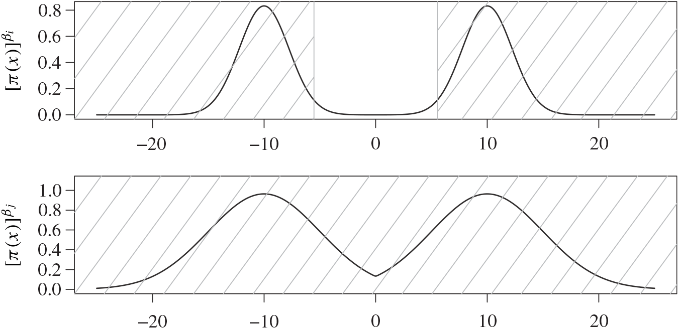
Figure 2: Plots of a simple bimodal Gaussian mixture distribution at two temperature levels
![]() $\beta_i$
and
$\beta_i$
and
![]() $\beta_j$
. The metric
$\beta_j$
. The metric
![]() $m(\cdot,\cdot)$
that allocates locations to mode points is chosen to be the Euclidean metric on
$m(\cdot,\cdot)$
that allocates locations to mode points is chosen to be the Euclidean metric on
![]() $\mathbb{R}$
. The shaded regions represent
$\mathbb{R}$
. The shaded regions represent
![]() $A_{ij}$
and
$A_{ij}$
and
![]() $A_{ji}$
in the top and bottom plots, respectively.
$A_{ji}$
in the top and bottom plots, respectively.
The aim is to use the transformation in a PT framework. So suppose that a temperature swap move proposal is made between two marginal components
![]() $x_i$
and
$x_i$
and
![]() $x_j$
at respective inverse temperatures
$x_j$
at respective inverse temperatures
![]() $\beta_i$
and
$\beta_i$
and
![]() $\beta_j$
with
$\beta_j$
with
![]() $\beta_i>\beta_j$
. The idea is that this swap move now utilises (7) so that the proposed move takes the form
$\beta_i>\beta_j$
. The idea is that this swap move now utilises (7) so that the proposed move takes the form
which to satisfy detailed balance is accepted with probability
Proposition 1
Consider a Markov chain that is in stationarity with a target distribution given by (1) on a state space
![]() $\mathcal{X}=\smash{\mathbb{R}^{(n+1)d}}$
. Let
$\mathcal{X}=\smash{\mathbb{R}^{(n+1)d}}$
. Let
![]() $\mu_1,\ldots,\mu_K \in
\mathbb{R}^d$
. If a temperature swap move of the form (8) is proposed where the transformation is given by (7) and is accepted with probability given in (9) then the chain is invariant with respect to (1).
$\mu_1,\ldots,\mu_K \in
\mathbb{R}^d$
. If a temperature swap move of the form (8) is proposed where the transformation is given by (7) and is accepted with probability given in (9) then the chain is invariant with respect to (1).
4. Quantile tempering algorithm (QuanTA)
The aim is to utilise the transformation-aided temperature swap moves in a PT algorithm. However, to perform the transformation, we need a collection of K centring points. Typically, these are unknown a priori and must be estimated. There are three obvious directions to proceed in: an involved optimisation process prior to the run of the algorithm that searches for mode points which are then fixed therein; an adaptive scheme that learns the mode points during the run of the algorithm; or a population Monte Carlo approach which discovers a collection of mode points using the most recent location of the Markov chain in a way that ensures that the Markov chain remains reversible.
Fixing the centring points prior to the run of the algorithm can be highly nonrobust since it leaves no scope to adjust in situations when new regions of mass are found during the run of the Markov chain. Also, it requires careful and potentially expensive precomputation.
Using adaptive techniques that ‘learn’ the best centring points are therefore preferable. However, adaptive MCMC approaches where the proposal mechanism adapts throughout the run of the algorithm [Reference Roberts and Rosenthal32], [Reference Roberts and Rosenthal33] requires careful design to ensure ergodicity. In contrast, the population MCMC approach essentially allows the proposal mechanism to adapt at every iteration without concerns about affecting the ergodicity, albeit typically at a computational cost which can be somewhat mitigated by exploiting computer parallelism.
The algorithm presented below utilises a population MCMC approach with N ‘copies’ of the PT approach to provide a large population of points in the state space that can be used in an appropriate clustering procedure to obtain a collection of K centring points, suggestions for which are given in Section 5.
4.1 The procedure
QuanTA runs the equivalent of N parallel tempering algorithm procedures in parallel with each single procedure using the same tempering schedule. With a temperature schedule given by
![]() $\Delta=\{
\beta_0,\ldots,\beta_n\}$
, the QuanTA approach can be seen as running a single Markov chain on the augmented state space,
$\Delta=\{
\beta_0,\ldots,\beta_n\}$
, the QuanTA approach can be seen as running a single Markov chain on the augmented state space,
![]() $${(\mathbb {R}{^d})^{n*N}}$$
. Letting
$${(\mathbb {R}{^d})^{n*N}}$$
. Letting
![]() ${\bf{x}}= \smash{(x_{(1,0)},\ldots,x_{(1,n)},x_{(2,0)},
\ldots,x_{(N,n)})}$
, the invariant target distribution for the Markov chain induced by QuanTA is
${\bf{x}}= \smash{(x_{(1,0)},\ldots,x_{(1,n)},x_{(2,0)},
\ldots,x_{(N,n)})}$
, the invariant target distribution for the Markov chain induced by QuanTA is
 $$\pi_Q({{\bf x}}) \propto \prod_{i=1}^N\pi_{\beta_0}(x_{(i,0)})
\pi_{\beta_1}(x_{(i,1)})\cdots\pi_{\beta_n}(x_{(i,n)} ).
$$
Initialisation. To initialise the QuanTA algorithm, we need to choose initial starting values for the Markov chain components, a suitable temperature schedule (see Theorem 1 in Section 6.2 for a suggested optimality criteria for the temperature schedule), the size of N, and suitable parameters for the chosen clustering method that will be used.
Running the chain. From the start point of the chain, QuanTA alternates between two types of Markov chain moves.
1. Within temperature Markov chain moves that use standard localised MCMC schemes for marginal updates of each of the $\smash{x_{(i,j)}}$
. Essentially, this is just Metropolis-within-Gibbs MCMC and in this setting, with hugely exploitable marginal independence, this process is highly parallelisable. Denote the $\pi_Q$
-invariant Markov transition kernel that performs temperature marginal updates on all components from a current point $ {{\bf x}} $
as $P_1({{\bf x}},{\rm d}{{\bf y}})$
.
$P_1({{\bf x}},{\rm d}{{\bf y}})$
.2. Temperature swap moves that propose to swap the chain locations between a pair of adjacent temperature components. This is where QuanTA differs from the standard PT procedure and uses the new transformation-aided temperature swap move detailed in Section 3.2, in particular in (7). This follows a two-phase population-MCMC update procedure.
Phase 1. Group marginal components into two collections,
 $$\begin{gather*}
C_1 = \big\{ x_{(i,j)}\colon i = 1,\ldots,
\big\lfloor{\tfrac{1}{2}N}\big\rfloor \text{ and } j=0,\ldots,n\big\},
\\
C_2 = \big\{ x_{(i,j)}\colon i =
\big(\big\lfloor{\tfrac{1}{2}N}\big\rfloor+1\big),\ldots,N \text{ and }
j=0,\ldots,n\big\}.
\end{gather*}$$
An appropriate clustering scheme (see Section 5) is performed on $C_1,$
providing a set of K centres $\{c_1,\ldots,c_K\}$
. To enhance the effectiveness of the transformation, it is suggested that these cluster centre points are used as initialisation locations for a suitable local optimisation procedure to find K mode points $M_1=\{\mu_1,\ldots,\mu_K\}$
of $\pi ({\cdot})$
(see Theorem 2 in Section 6.2).
$\pi ({\cdot})$
(see Theorem 2 in Section 6.2).For each $i \in \{(\lfloor*{N/2}\rfloor+1),\ldots,N \}$
, sample
 $l \sim {\rm
Unif}\{0,1,\ldots,n-1\}$
and select the corresponding pair of adjacent temperature marginals $\smash{(x_{(i,l)},x_{(i,l+1)})}$
for a temperature swap move proposal utilising the transformation from (7) (which is centred on the associated point from $M_1$
). This move is accepted with probability (9).
$M_1$
). This move is accepted with probability (9).Phase 2. Repeat phase 1, but with the roles of $C_1$
and $C_2$
reversed.
Denote the
![]() $\pi_Q$
-invariant Markov transition kernel that implements this temperature swap update procedure for all components using the above two-phase process by
$\pi_Q$
-invariant Markov transition kernel that implements this temperature swap update procedure for all components using the above two-phase process by
![]() $P_2({{\bf x}},{\rm d}{{\bf y}})$
.
$P_2({{\bf x}},{\rm d}{{\bf y}})$
.
From the initialisation point
![]() $${\mathbf {x}}$$
, the Markov chain output is created by application of the kernel compilation
$${\mathbf {x}}$$
, the Markov chain output is created by application of the kernel compilation
where k is the user-chosen number of within temperature Markov chain updates between each swap move proposal and T is the user-chosen number of iterations of the algorithm before stopping.
Remark 1
By Proposition 1, the transformation-aided temperature swap move established in Section 3.2 leaves the Markov chain constructed by QuanTA
![]() $\pi_Q({\cdot})$
invariant. Provided that appropriate within-temperature MCMC moves are utilised then QuanTA establishes an irreducible and aperiodic
$\pi_Q({\cdot})$
invariant. Provided that appropriate within-temperature MCMC moves are utilised then QuanTA establishes an irreducible and aperiodic
![]() $\pi_Q({\cdot})$
invariant Markov chain as required [Reference Tierney42].
$\pi_Q({\cdot})$
invariant Markov chain as required [Reference Tierney42].
Remark 2
Although not made explicit in the notation above, the transformation centring points,
![]() $\{\mu_1,\ldots,\mu_K \}$
, are repeatedly estimated from subsets of the points in the population of the N replicate PT schemes. As such, their values are not fixed and have flexibility to change and adapt accordingly with the population. This is a major bonus of the population MCMC framework for a multimodal problem, allowing powerful and robust adaptation when new regions of mass are discovered.
$\{\mu_1,\ldots,\mu_K \}$
, are repeatedly estimated from subsets of the points in the population of the N replicate PT schemes. As such, their values are not fixed and have flexibility to change and adapt accordingly with the population. This is a major bonus of the population MCMC framework for a multimodal problem, allowing powerful and robust adaptation when new regions of mass are discovered.
5. Estimating local mode locations
The QuanTA algorithm, presented in Section 4, requires online estimation of the local mode points as centring locations for the transformation. In this section we outline a practical scheme that is used in the canonical simulation studies.
With a typically unknown number of modes and a population of chains, a principled approach would be to fit a Dirichlet process mixture model, e.g. [Reference Kim, Tadesse and Vannucci15] and [Reference Neal22]. A comprehensive Gibbs sampling approach for this can be computationally expensive, but there are alternative cheaper but approximate methods that are left for exploration in further work [Reference Raykov, Boukouvalas and Little29].
For the examples with well-separated modes that were studied here, it sufficed to use a cheap and fast clustering scheme [Reference Hastie, Tibshirani and Friedman13]. To this end, a K-means approach was used [Reference Hartigan and Wong11], where although the theoretical computational complexity is NP-hard in full generality, when in a setting with well-separated clusters, the algorithm rapidly reaches a good solution as the problem is much easier.
The clustering procedure provides a collection of cluster centres that can be directly used as centring points for the transformation or as very useful initialisation points for a local optimisation method. Indeed, Theorem 2 of Section 6 shows that QuanTA can achieve accelerated mixing through the temperature levels when the centring point is chosen as the mode point, particularly at colder temperatures when the Gaussian approximation to the mode becomes increasingly accurate; see, e.g. [Reference Barndorff-Nielsen and Cox2] and [Reference Olver24].
5.1 A weighted K-means clustering
Typically, the K-means algorithm assigns all points equal leverage in determining cluster centres. A weighted K-means approach incorporates weights that can alter the leverages of points. In the tempering setting chains at the colder states, where the modes are less disperse, should have more leverage in determining the centres.
Weighted K means is an almost identical procedure to the K-means algorithm of [Reference Hartigan and Wong11] but now incorporates the weights to give points leverage. For the setting of interest, each chain location will be allocated a weight, determined by their inverse temperature value. So, for a collection of
![]() $\nu$
chain locations
$\nu$
chain locations
![]() $x_1,\ldots, x_\nu$
at inverse temperature levels,
$x_1,\ldots, x_\nu$
at inverse temperature levels,
![]() $\beta_{x_1},\ldots,\beta_{x_\nu}$
form their respective weights.
$\beta_{x_1},\ldots,\beta_{x_\nu}$
form their respective weights.
The weighted K-means algorithm gives a pragmatic way of creating a plausible particle allocation,
![]() $\smash{\hat{S}}$
, in to K partitions. Denoting a partition S by
$\smash{\hat{S}}$
, in to K partitions. Denoting a partition S by
![]() $S= \{S_1,\ldots,S_K \}$
, where
$S= \{S_1,\ldots,S_K \}$
, where
![]() $S_j \subset \{ x_1,\ldots, x_\nu \}$
, then the procedure aims to establish an allocation,
$S_j \subset \{ x_1,\ldots, x_\nu \}$
, then the procedure aims to establish an allocation,
![]() $\hat{S}$
, such that
$\hat{S}$
, such that
 $$\hat{S}=\mbox{argmin}_{S} \bigg\{ \sum_{i=1}^M \sum_{j=1}^\nu {\bf
1}_{\{x_j\in S_i\}} \beta_{x_j} ||x_j-\mu_{i}||^2 \bigg\}.$$
The weighted K-means algorithm begins with an initial set of K centres
![]() $\{\mu_1,\ldots,\mu_K\}$
. It then proceeds by alternating between two updating steps until point allocations do not change (signaling a minimum of or a pre-specified number of iterations is reached); a point allocation step, where each point x is assigned to the set
$\{\mu_1,\ldots,\mu_K\}$
. It then proceeds by alternating between two updating steps until point allocations do not change (signaling a minimum of or a pre-specified number of iterations is reached); a point allocation step, where each point x is assigned to the set
![]() $S_j,$
where
$S_j,$
where
![]() $j=\text{arg min}_j ||x-\mu_{j}||^2$
; a centre point update step, where, for the new allocation, the centring points are each updated to be the weighted mean of their respective component steps, i.e.
$j=\text{arg min}_j ||x-\mu_{j}||^2$
; a centre point update step, where, for the new allocation, the centring points are each updated to be the weighted mean of their respective component steps, i.e.
The weighted K-means procedure (see, e.g. [Reference Kerdprasop, Kerdprasop and Sattayatham14] and [Reference Tseng44]) can be implemented using the R package‘FactoClass’ by Pardo and Del Campo [Reference Pardo and Del Campo27], which uses a modified version of the K-means algorithm of Hartigan and Wong [Reference Hartigan and Wong11].
6. Theoretical underpinnings of QuanTA in high dimensions
In both QuanTA and the PT algorithms, the acceptance of temperature swap proposals allow the transfer of hot-state mixing information to be passed through to the cold state. The ambitiousness of the spacings between the consecutive inverse temperatures dictate the performance of the algorithm. Similarly to the problem of tuning the RWM algorithm [Reference Roberts, Gelman and Gilks35], we seek the optimal balance between over- and under-ambitious proposals. This issue becomes increasingly problematic with an increase in dimensionality; hence, careful scaling of the consecutive temperature spacings is needed to prevent degeneracy of acceptance rates.
The work in [Reference Atchadé, Roberts and Rosenthal1] sought an optimal scaling result for temperature spacings in a PT algorithm. This section takes a similar approach to derive an equivalent result for QuanTA. It will be shown in Theorem 1 that consecutive spacings inducing swap rates of approximately 0.234 are optimal, thus giving guidance for practitioners to tune towards an optimal setup. Complementary to this, Theorem 2 justifies the use of QuanTA outside the Gaussian setting, showing that, under mild conditions, the transformation move allows for larger spacings in the temperature schedule than the PT algorithm does.
6.1 Optimal scaling of QuanTA—the setup and assumptions
As the dimensionality d of the target distribution tends to infinity, the problem of selecting temperature spacings for QuanTA is investigated. Suppose that a swap move between two consecutive temperature levels
![]() $\beta$
and
$\beta$
and
![]() $\beta'=\beta+\epsilon$
for some
$\beta'=\beta+\epsilon$
for some
![]() $\epsilon>0$
is proposed. As in [Reference Atchadé, Roberts and Rosenthal1], the measure of the efficiency of the inverse temperature spacing will be the expected squared jumping distance,
$\epsilon>0$
is proposed. As in [Reference Atchadé, Roberts and Rosenthal1], the measure of the efficiency of the inverse temperature spacing will be the expected squared jumping distance,
![]() ${\rm ESJD}_\beta$
, defined as
${\rm ESJD}_\beta$
, defined as
where
![]() $\gamma=\beta+\epsilon$
if the proposed swap is accepted and
$\gamma=\beta+\epsilon$
if the proposed swap is accepted and
![]() $\gamma=\beta$
otherwise. Note the assumption that the Markov chain has reached invariance and so the expectation is taken with respect to the invariant distribution
$\gamma=\beta$
otherwise. Note the assumption that the Markov chain has reached invariance and so the expectation is taken with respect to the invariant distribution
![]() $\pi_n({\cdot})$
.
$\pi_n({\cdot})$
.
The
![]() ${\rm ESJD}_\beta$
is a natural quantity to consider ([Reference Sherlock38]) since maximising this would appear to ensure that one is being sufficiently ambitious with spacings but not inducing degenerate acceptance rates. However, it is worth noting that it is only truly justified when there is an associated diffusion limit for the chain; see [Reference Roberts and Rosenthal34].
${\rm ESJD}_\beta$
is a natural quantity to consider ([Reference Sherlock38]) since maximising this would appear to ensure that one is being sufficiently ambitious with spacings but not inducing degenerate acceptance rates. However, it is worth noting that it is only truly justified when there is an associated diffusion limit for the chain; see [Reference Roberts and Rosenthal34].
The aim is to establish the limiting behaviour of the
![]() ${\rm ESJD}_\beta$
as
${\rm ESJD}_\beta$
as
![]() $d\rightarrow \infty$
and then optimise this limiting form. To this end, for tractability, the form of the d-dimensional target is restricted to distributions of the form
$d\rightarrow \infty$
and then optimise this limiting form. To this end, for tractability, the form of the d-dimensional target is restricted to distributions of the form
 $$\begin{equation}
\pi(x) \propto f_d(x) = \prod_{i=1}^d f(x_i),
\label{eqn11}
\end{equation}
$$
and to achieve a nondegenerate acceptance rate as
![]() $d \rightarrow \infty$
the spacings are necessarily scaled as
$d \rightarrow \infty$
the spacings are necessarily scaled as
![]() $\mathcal{O}(d^{-1/2})$
, i.e.
$\mathcal{O}(d^{-1/2})$
, i.e.
where
![]() $\ell$
a positive constant that one tunes to attain an optimal
$\ell$
a positive constant that one tunes to attain an optimal
![]() ${\rm ESJD}_\beta$
.
${\rm ESJD}_\beta$
.
Furthermore, assume that the univariate marginal components
![]() $f({\cdot})$
are
$f({\cdot})$
are
![]() $C^4$
and have a global maxima at
$C^4$
and have a global maxima at
![]() $\mu$
, i.e.
$\mu$
, i.e.
The point
![]() $\mu$
is the centring point for the transformation-aided temperature swap move analysed in the forthcoming Theorem 1. Note that the result of Theorem 1 still holds even if
$\mu$
is the centring point for the transformation-aided temperature swap move analysed in the forthcoming Theorem 1. Note that the result of Theorem 1 still holds even if
![]() $\mu$
is chosen as an arbitrary point in the state space. However, the global mode point
$\mu$
is chosen as an arbitrary point in the state space. However, the global mode point
![]() $\mu$
is the canonical transformation centring point, as will be seen in the subsequent result in Theorem 2.
$\mu$
is the canonical transformation centring point, as will be seen in the subsequent result in Theorem 2.
Furthermore, the marginal components
![]() $f({\cdot})$
are assumed to be of the form
$f({\cdot})$
are assumed to be of the form
where
![]() $H(x)\,{:\!=}\,{-}\,\log(f(x))$
is regularly varying [Reference Bingham, Goldie and Teugels3], i.e. there exists an
$H(x)\,{:\!=}\,{-}\,\log(f(x))$
is regularly varying [Reference Bingham, Goldie and Teugels3], i.e. there exists an
![]() $\alpha >0$
such that, for
$\alpha >0$
such that, for
![]() $x>0$
,
$x>0$
,
This is a sufficient condition for Theorem 1 and ensures that the moments and integrals required for the proof are all well defined. Furthermore, assume that the fourth derivatives of
![]() $(\log
f)({\cdot})$
are bounded, i.e. there exists an
$(\log
f)({\cdot})$
are bounded, i.e. there exists an
![]() $M>0$
such that
$M>0$
such that
This condition is sufficient for proving Theorem 1 but not necessary. The proof still works if the condition is weakened so that, for some
![]() $k\ge 4,$
the kth derivative of the logged density is bounded.
$k\ge 4,$
the kth derivative of the logged density is bounded.
Finally, for notational convenience, the following are defined, with the subscript
![]() $\beta$
indicating that the expectation is with respect to
$\beta$
indicating that the expectation is with respect to
![]() $f^\beta ({\cdot})$
:
$f^\beta ({\cdot})$
:
 $$\begin{align*}
V(\beta)&= \frac{1}{\beta^2},
\\
I(\beta)&={\rm var}_{\beta}[(\log f)(x)],
\\
R(\beta)&= \mathbb{E}_{\beta}[(x-\mu)^2(\log f)''(x)-(x-\mu)(\log
f)'(x)].
\end{align*}
$$
Theorem 1 below deals with a single-mode setting which is a very good approximation of a multimodal setting with homogeneous modal structure and where the mode weights remain stable at consecutive temperatures [Reference Tawn and Roberts40], [Reference Woodard, Schmidler and Huber48]. Outside this setting other methods are needed to stabilise the modal weights at different temperatures [Reference Tawn, Roberts and Rosenthal41]; then the QuanTA transformation-aided swap moves can be successfully utilised alongside such an approach.
Since we assume only one transformation-centring point, there is a simplified form of the acceptance probability that no longer requires the indicator functions. Denote the acceptance probability of the QuanTA-style swap move by
![]() $\alpha_{\beta}(x,y),$
so
$\alpha_{\beta}(x,y),$
so
 $$\begin{equation}
\alpha_{\beta}(x,y)=\mbox{min}\bigg(1, \frac{f_d^{\beta'}
(g(x,\beta,\beta^{'})) f_d^{\beta}(g(\,y,\beta^{'},\beta))}{f_d^{\beta'}
(\,y)f_d^{\beta}(x)} \bigg).
\label{eqn16}
\end{equation}
$$
Then a simple calculation shows that the
![]() ${\rm ESJD}_\beta$
from (10) becomes
${\rm ESJD}_\beta$
from (10) becomes
which will be maximised with respect to
![]() $\ell$
in the limit as
$\ell$
in the limit as
![]() $d\rightarrow \infty$
.
$d\rightarrow \infty$
.
6.2 Scaling results and interpretation
Under the setting of Section 6.1 and with
![]() $\Phi({\cdot})$
denoting the CDF of a standard Gaussian, the following optimal scaling result is derived.
$\Phi({\cdot})$
denoting the CDF of a standard Gaussian, the following optimal scaling result is derived.
Theorem 1
(Optimal scaling for the QuanTA algorithm.) Consider QuanTA targeting a distribution
![]() $\pi({\cdot})$
satisfying (11). Assume that the marginal components
$\pi({\cdot})$
satisfying (11). Assume that the marginal components
![]() $f({\cdot})$
satisfy (12), are regularly varying satisfying (13) and (14), and that
$f({\cdot})$
satisfy (12), are regularly varying satisfying (13) and (14), and that
![]() $\log f({\cdot})$
satisfies (15). Assuming that
$\log f({\cdot})$
satisfies (15). Assuming that
![]() $\epsilon = \ell /
d^{1/2}$
for some
$\epsilon = \ell /
d^{1/2}$
for some
![]() $\ell\in \mathbb{R}_{+}$
then in the limit as
$\ell\in \mathbb{R}_{+}$
then in the limit as
![]() $d\rightarrow\infty$
, the
$d\rightarrow\infty$
, the
![]() ${\rm ESJD}_{\beta}$
, given in (17) is maximised when
${\rm ESJD}_{\beta}$
, given in (17) is maximised when
![]() $\ell$
is chosen to maximise
$\ell$
is chosen to maximise
Furthermore, for the optimal
![]() $\ell,$
the corresponding swap move acceptance rate induced between two consecutive temperatures is given by 0.234 (to three significant figures).
$\ell,$
the corresponding swap move acceptance rate induced between two consecutive temperatures is given by 0.234 (to three significant figures).
Proof. The details of the proof of Theorem 1 are deferred to Appendix A. The strategy comprises three key stages: establishing a Taylor series expansion of the logged swap move acceptance ratio (i.e. the log of (16)); establishing limiting Gaussianity of this logged acceptance ratio; and, finally, achieving a tractable form of the limiting
![]() ${\rm ESJD}_{\beta}$
which is then optimised with respect to
${\rm ESJD}_{\beta}$
which is then optimised with respect to
![]() $\ell,$
giving rise to an associated optimal acceptance rate.
$\ell,$
giving rise to an associated optimal acceptance rate.
Remark 3
In the special case that the marginal targets are Gaussian, i.e.
![]() $f(x) =
\phi(x; \mu, \sigma^2),$
then the transformation swap move should permit arbitrarily ambitious spacings. This is verified by observing that in this case
$f(x) =
\phi(x; \mu, \sigma^2),$
then the transformation swap move should permit arbitrarily ambitious spacings. This is verified by observing that in this case
and so, with respect to
![]() $\ell,$
(18) becomes proportional to
$\ell,$
(18) becomes proportional to
![]() $\ell^2$
which has no finite maximal value; thus demonstrating consistency with what is know in the Gaussian case.
$\ell^2$
which has no finite maximal value; thus demonstrating consistency with what is know in the Gaussian case.
Remark 4
The optimality criterion given in (18) is very similar to that derived in [Reference Atchadé, Roberts and Rosenthal1] and [Reference Roberts and Rosenthal34]. Indeed, both QuanTA and the PT algorithm require the same dimensionality spacing scaling, and both are optimised when a 0.234 acceptance rate is induced. However, there will be a difference in the behaviour of the optimal
![]() $\hat{\ell},$
which is where QuanTA can be shown to give accelerated mixing versus the PT approach; see Theorem 2 below.
$\hat{\ell},$
which is where QuanTA can be shown to give accelerated mixing versus the PT approach; see Theorem 2 below.
Remark 5
Theorem 1 gives an explicit formula for derivation of the optimal
![]() $\hat{\ell}$
between consecutive temperatures, but this is usually intractable in a real problem. However, for a practitioner, the associated 0.234 optimal swap acceptance rate gives useful setup guidelines. In fact, the theorem suggests a strategy for optimal setup starting with a chain at the hottest level and tuning the spacing to successively colder temperature levels based on the swap acceptance rate to attain consecutive swap rates close to 0.234. Indeed, using a stochastic approximation algorithm (see [Reference Robbins and Monro30]), Miasojedow et al. [Reference Miasojedow, Moulines and Vihola19] took an adaptive MCMC approach [Reference Roberts and Rosenthal33] to do this for the PT algorithm, but their framework also extends naturally to QuanTA.
$\hat{\ell}$
between consecutive temperatures, but this is usually intractable in a real problem. However, for a practitioner, the associated 0.234 optimal swap acceptance rate gives useful setup guidelines. In fact, the theorem suggests a strategy for optimal setup starting with a chain at the hottest level and tuning the spacing to successively colder temperature levels based on the swap acceptance rate to attain consecutive swap rates close to 0.234. Indeed, using a stochastic approximation algorithm (see [Reference Robbins and Monro30]), Miasojedow et al. [Reference Miasojedow, Moulines and Vihola19] took an adaptive MCMC approach [Reference Roberts and Rosenthal33] to do this for the PT algorithm, but their framework also extends naturally to QuanTA.
6.2.1 Higher-order scalings at cold temperatures
For any univariate Gaussian distribution at inverse temperature level
![]() $\beta$
,
$\beta$
,
![]() $I(\beta)=1/(2\beta^2)$
. It was shown in [Reference Atchadé, Roberts and Rosenthal1] that the optimal choice for the scaling parameter takes the form
$I(\beta)=1/(2\beta^2)$
. It was shown in [Reference Atchadé, Roberts and Rosenthal1] that the optimal choice for the scaling parameter takes the form
resulting in a geometrically spaced temperature schedule.
Assuming appropriate smoothness for the marginal components
![]() $f({\cdot})$
, for a sufficiently cold temperature, the local mode can be well approximated by a Gaussian [Reference Tierney and Kadane43]. So, for sufficiently cold temperatures (i.e. large
$f({\cdot})$
, for a sufficiently cold temperature, the local mode can be well approximated by a Gaussian [Reference Tierney and Kadane43]. So, for sufficiently cold temperatures (i.e. large
![]() $\beta$
), we expect
$\beta$
), we expect
![]() $I\,(\beta)
\approx 1/(2\beta^2)$
, thus spacings become (approximately)
$I\,(\beta)
\approx 1/(2\beta^2)$
, thus spacings become (approximately)
![]() $\mathcal{O}(\beta)$
(note that a rigorous derivation that
$\mathcal{O}(\beta)$
(note that a rigorous derivation that
![]() $I\,(\beta)
\approx 1/(2\beta^2)$
is contained in the proof of Theorem 2). Defining the ‘order of the spacing with respect to the inverse temperature
$I\,(\beta)
\approx 1/(2\beta^2)$
is contained in the proof of Theorem 2). Defining the ‘order of the spacing with respect to the inverse temperature
![]() $\beta$
’ as the value of
$\beta$
’ as the value of
![]() $\zeta$
such that the optimal spacing is
$\zeta$
such that the optimal spacing is
![]() $\mathcal{O}(\beta^\zeta),$
then the standard PT algorithm is order 1 for sufficiently cold temperatures.
$\mathcal{O}(\beta^\zeta),$
then the standard PT algorithm is order 1 for sufficiently cold temperatures.
In the Gaussian setting, QuanTA exhibits ‘infinitely’ high-order behaviour since there is no restriction on the size of the temperature spacings with regards the value of
![]() $\beta$
. It is hoped that some of this higher-order behaviour is inherited in a more general target distribution setting when the modes can be considered to be sufficiently close to Gaussian.
$\beta$
. It is hoped that some of this higher-order behaviour is inherited in a more general target distribution setting when the modes can be considered to be sufficiently close to Gaussian.
It will be seen in Theorem 2 below that, under the setting of Theorem 1 but with a single additional condition, QuanTA does exhibit higher-order behaviour than the PT algorithm at cold temperatures.
With
![]() $f({\cdot})$
as in Theorem 1 (but now, without loss of generality, the mode point is at
$f({\cdot})$
as in Theorem 1 (but now, without loss of generality, the mode point is at
![]() $\mu=0$
), define the normalised density
$\mu=0$
), define the normalised density
![]() $g_\beta({\cdot})$
as
$g_\beta({\cdot})$
as
The additional assumption required to prove the higher-order behaviour of QuanTA is that there exists
![]() $\gamma>0$
such that, as
$\gamma>0$
such that, as
![]() $\beta\rightarrow
\infty$
,
$\beta\rightarrow
\infty$
,
This assumption essentially guarantees the convergence to Gaussianity about the mode as
![]() $\beta\rightarrow\infty$
. This assumption appears to be reasonable with studies of both gamma and student-t distributions, demonstrating a value of
$\beta\rightarrow\infty$
. This assumption appears to be reasonable with studies of both gamma and student-t distributions, demonstrating a value of
![]() $\gamma=1$
; details can be found in [Reference Tawn39].
$\gamma=1$
; details can be found in [Reference Tawn39].
Theorem 2
(Cold temperature scalings.) For marginal targets
![]() $f({\cdot})$
satisfying the conditions of Theorem 1 and (19), for sufficiently large
$f({\cdot})$
satisfying the conditions of Theorem 1 and (19), for sufficiently large
![]() $\beta$
,
$\beta$
,
where $k=\min\{2+\gamma, 3 \}>2$
if f is symmetric about the mode point 0, $k=\min\{2+\gamma, \smash{\tfrac{5}{2}} \}>2$
otherwise.
This induces an optimising value
![]() $\hat{\ell}$
such that
$\hat{\ell}$
such that
showing that at the colder temperatures QuanTA permits higher-order behaviour than the standard PT scheme which has
![]() $\hat{\ell}=
\mathcal{O}(\beta)$
.
$\hat{\ell}=
\mathcal{O}(\beta)$
.
Proof. Since the optimal
![]() $\ell$
derived in Theorem 1 is given by
$\ell$
derived in Theorem 1 is given by
the proof of Theorem 2 follows immediately if it can be shown that
Indeed, two key lemmata are derived in Appendix A.2: Lemma 4 establishes that
![]() $\smash{\tfrac{1}{2}} V(\beta)
-I(\beta)=\mathcal{O}({1}/{\beta^k})$
and Lemma 5 establishes that
$\smash{\tfrac{1}{2}} V(\beta)
-I(\beta)=\mathcal{O}({1}/{\beta^k})$
and Lemma 5 establishes that
![]() $R(\beta)/{4\beta}=\mathcal{O}({1}/{\beta^k})$
. Thus, the result in (20) holds and the proof is complete.
$R(\beta)/{4\beta}=\mathcal{O}({1}/{\beta^k})$
. Thus, the result in (20) holds and the proof is complete.
Remark 6
Theorem 2 studies the behaviour of the optimal spacings for large values of
![]() $\beta$
, where
$\beta$
, where
![]() $\beta$
is larger than 1. Even though the QuanTA and PT approaches use temperatures in the range [0,1], the result still proves insightful in many situations that QuanTA can encounter.
$\beta$
is larger than 1. Even though the QuanTA and PT approaches use temperatures in the range [0,1], the result still proves insightful in many situations that QuanTA can encounter.
This is due to the arbitrary nature of the ‘
![]() $\beta=1$
’ temperature level which is a result of the tempering being relative rather than absolute for the modes. Hence, the modes of the target distribution of interest may exhibit a within mode structure that makes it appear that a mode has been cooled to an inverse temperature much larger than 1.
$\beta=1$
’ temperature level which is a result of the tempering being relative rather than absolute for the modes. Hence, the modes of the target distribution of interest may exhibit a within mode structure that makes it appear that a mode has been cooled to an inverse temperature much larger than 1.
As an example, take a Gamma(
![]() $\alpha,\gamma$
) distribution, where, for some
$\alpha,\gamma$
) distribution, where, for some
![]() $\alpha>0$
,
$\alpha>0$
,
![]() $\gamma>0,$
and
$\gamma>0,$
and
![]() $x>0$
,
$x>0$
,
Then, with slight abuse of notation,
![]() $f^{\beta^{*}}\sim{\rm Gamma}(\alpha
\beta^{*}-\beta^{*} +1, \gamma \beta^{*}$
). Suppose that the target distribution of interest was given by
$f^{\beta^{*}}\sim{\rm Gamma}(\alpha
\beta^{*}-\beta^{*} +1, \gamma \beta^{*}$
). Suppose that the target distribution of interest was given by
![]() $\pi \sim f^{\beta^{*}}$
and one raises
$\pi \sim f^{\beta^{*}}$
and one raises
![]() $\pi$
to a power
$\pi$
to a power
![]() $\beta<1$
. Then
$\beta<1$
. Then
![]() $\pi^{\beta}\sim{\rm
Gamma}(\alpha \beta\beta^{*}-\beta\beta^{*} +1, \gamma \beta\beta^{*})$
. Thus, if
$\pi^{\beta}\sim{\rm
Gamma}(\alpha \beta\beta^{*}-\beta\beta^{*} +1, \gamma \beta\beta^{*})$
. Thus, if
![]() $\beta^{*}$
is large and
$\beta^{*}$
is large and
![]() $\beta<1$
is such that
$\beta<1$
is such that
![]() $\beta
\beta^{*}$
remains large, then one is in the setting of Theorem 2.
$\beta
\beta^{*}$
remains large, then one is in the setting of Theorem 2.
Furthermore, ongoing work is hoping to develop novel methodology for sampling from multimodal distributions that utilises temperature levels with
![]() $\beta>1$
where necessarily
$\beta>1$
where necessarily
![]() $\beta \rightarrow \infty$
as
$\beta \rightarrow \infty$
as
![]() $d\rightarrow \infty$
. The results established here are directly applicable to that work.
$d\rightarrow \infty$
. The results established here are directly applicable to that work.
Remark 7
The result in Theorem 2 does not imply that QuanTA is not useful outside the Gaussian or super cold settings. The QuanTA approach will be practically useful in settings where the mode can be well approximated by a Gaussian and thus the transformation in the transformation-aided swap move approximately preserves the mode’s CDF. What Theorem 2 does show is that, for a large class of distributions that exhibit appropriate smoothness, QuanTA is sensible, and is arguably the canonical approach to take at the colder temperature levels, since it enables accelerated mixing speed through the temperature schedule.
7. Examples of implementation
In this section we give illustrative examples for the canonical setting of a Gaussian mixture to illustrate the potential gains of QuanTA over the standard PT approach.
The QuanTA transformation move does not solve all the issues inherent in the PT framework. This will be highlighted with the final example in this section. In fact, Woodard et al. [Reference Woodard, Schmidler and Huber47], [Reference Woodard, Schmidler and Huber48] showed that, for most ‘interesting’ examples, the mixing speed decays exponentially slowly with dimension. Prototype approaches to navigating this problem can be found in [Reference Tawn39] and [Reference Tawn, Roberts and Rosenthal41]. Also, note that the examples all focus on the setting when the target distribution is a Gaussian mixture, which is often a good approximation to a range of multimodal distributions. Outside the setting of Gaussian modes the transformation-aided swap move will not be as effective since the within-mode CDF preservation transformation will only be an approximation to preservation of the CDF.
In each of the examples given, both the new QuanTA and standard (PT) parallel schemes will be run for comparison of performance. In all examples the following applies.
1. Both the new QuanTA and PT versions were run 10 times to ensure replicability.
2. Both the PT and QuanTA algorithms were run so that 20 000 swap moves would be attempted. For QuanTA, this would be 20 000 swaps for each of the N individual parallel tempering schemes in parallel of which there were $N=100$
in this example. Also, all schemes had the same within to swap move ratio $(3\colon \!1)$
.
$(3\colon \!1)$
.3. Both versions use the same set of (geometrically generated) temperature spacings, chosen to be overly ambitious for the PT setup but demonstrably under ambitious for the new QuanTA scheme.
4. Also presented is the optimal temperature schedule for the PT setup generated under the optimal acceptance rate of 0.234 for the PT algorithm suggested in [Reference Atchadé, Roberts and Rosenthal1]. This demonstrates the extra complexity needed to produce a functioning algorithm for the PT approach.
5. For all runs, the within temperature level proposals were made with Gaussian RWM moves tuned to an optimal 0.234 acceptance rate (see [Reference Roberts, Gelman and Gilks35]).
7.1 One-dimensional example
The target distribution given by
 $$\begin{equation}
\pi(x) \propto \sum_{k=1}^5 w_k \phi(x\ ;\ \mu_k,\sigma^2),
\label{eqn21}
\end{equation}
$$
where
![]() $\phi(\cdot;\mu,\sigma^2)$
is the density function of a univariate Gaussian with mean
$\phi(\cdot;\mu,\sigma^2)$
is the density function of a univariate Gaussian with mean
![]() $\mu$
and variance
$\mu$
and variance
![]() $\sigma^2$
. In this example,
$\sigma^2$
. In this example,
![]() $\sigma=0.01$
, the mode centres are given by
$\sigma=0.01$
, the mode centres are given by
![]() $$(\mu_{1},\mu_{2},\mu_{3},\mu_{4},\mu_{5})=(-200,-100,0,100,200)$$
and all modes are equally weighted with
$$(\mu_{1},\mu_{2},\mu_{3},\mu_{4},\mu_{5})=(-200,-100,0,100,200)$$
and all modes are equally weighted with
![]() $w_1=w_2=\cdots=w_5$
.
$w_1=w_2=\cdots=w_5$
.
The temperature schedule for this example is given by a geometric schedule with an ambitious
![]() $0.0002$
common ratio for the spacings. Only three levels are used and so the temperature schedule is given by
$0.0002$
common ratio for the spacings. Only three levels are used and so the temperature schedule is given by
![]() $\Delta=\{ 1,0.0002,0.0002^2 \}$
; see Figure 3.
$\Delta=\{ 1,0.0002,0.0002^2 \}$
; see Figure 3.
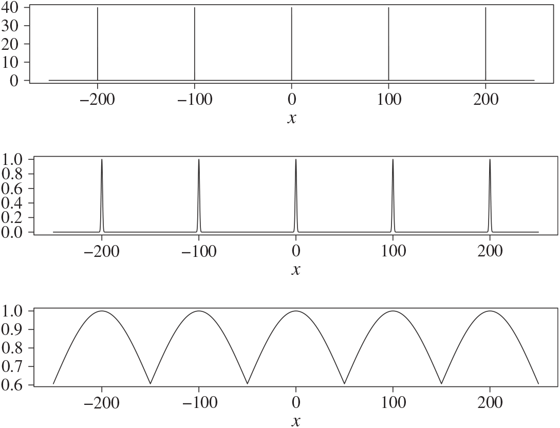
Figure 3: The (non-normalised) tempered target distributions for (21) for inverse temperatures
![]() $\Delta=\{
1,0.0002,0.0002^2 \},$
respectively.
$\Delta=\{
1,0.0002,0.0002^2 \},$
respectively.
In all runs all the chains were started from a start location of
![]() $-200$
. In Figure 1, from the introductory section, we presented two representative trace plots of the target state chain for a run of the PT algorithm and a single scheme from QuanTA. There is a clear improvement in the inter-modal mixing for the QuanTA.
$-200$
. In Figure 1, from the introductory section, we presented two representative trace plots of the target state chain for a run of the PT algorithm and a single scheme from QuanTA. There is a clear improvement in the inter-modal mixing for the QuanTA.
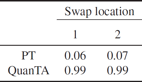
In Table 1 we give the associated acceptance rates. Clearly, the rate of transfer of mixing information from the hot states to the cold state is significantly higher for QuanTA.
Table 1: Comparison of the acceptance rates of swap moves for the PT algorithm and QuanTA targeting the one-dimensional distribution given in (21) and setup with the ambitious inverse temperature schedule given by
![]() $\Delta=\{ 1,0.0002,0.0002^2
\}$
.
$\Delta=\{ 1,0.0002,0.0002^2
\}$
.
In Figure 4 we compare the running modal weight approximation for the mode centred on 200 when using the standard PT and QuanTA schemes. This used the cold state chains from 10 individual runs of the PT algorithm and 10 single schemes selected randomly from 10 separate runs of the QuanTA algorithm.
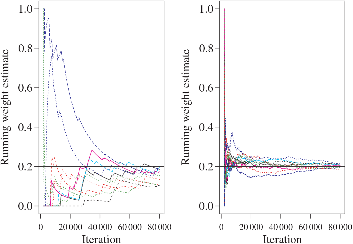
Figure 4: For the target given in (21), the running weight approximations for the mode centred on 200 with target weight
![]() $w_5=0.2$
for 10 separate runs of the PT and QuanTA schemes. Left: the PT runs showing slow and variable estimates for
$w_5=0.2$
for 10 separate runs of the PT and QuanTA schemes. Left: the PT runs showing slow and variable estimates for
![]() $w_5$
. Right: the new QuanTA scheme showing fast, unbiased convergence to the true value for
$w_5$
. Right: the new QuanTA scheme showing fast, unbiased convergence to the true value for
![]() $w_5$
.
$w_5$
.
Denoting the estimator of the kth mode’s weight by
![]() $\hat{w_k}$
and the respective cold state chain’s ith value as
$\hat{w_k}$
and the respective cold state chain’s ith value as
![]() $X_i$
,
$X_i$
,
 $$\label{eq:weightreparamest}
\hat{w_k} = \frac{1}{N-B+1}\sum_{i=B}^N{\bf 1}_{\{ c_k\le X_i\le C_k\}},
$$
where
![]() $c_k$
and
$c_k$
and
![]() $C_k$
are the chosen upper and lower boundary points for allocation to the kth mode, and B is the length of the burn-in removed.
$C_k$
are the chosen upper and lower boundary points for allocation to the kth mode, and B is the length of the burn-in removed.
Figure 4 reveals that the QuanTA approach has a vastly improved rate of convergence; with the PT runs still exhibiting bias from the chain initialisation locations.
An interesting comparison between the approaches is to observe how many extra temperature levels would be required to make the PT scheme work optimally (i.e. with consecutive 0.234 swap acceptance rates). This gives a clearer idea of the reduction in the number of intermediate levels that can be achieved using the QuanTA.
With the same hottest state level of
![]() $\beta=0.0002^2$
, a geometrical inverse temperature schedule was tuned to give a swap rate of approximately 0.234 between consecutive levels for the PT algorithm in this example. In fact, a 0.04 geometric ratio suggested optimality for the PT scheme. Hence, to reach the stated hottest level, seven temperatures are needed, as opposed to the three that were evidently unambitious for QuanTA.
$\beta=0.0002^2$
, a geometrical inverse temperature schedule was tuned to give a swap rate of approximately 0.234 between consecutive levels for the PT algorithm in this example. In fact, a 0.04 geometric ratio suggested optimality for the PT scheme. Hence, to reach the stated hottest level, seven temperatures are needed, as opposed to the three that were evidently unambitious for QuanTA.
7.2 Twenty-dimensional example
The target distribution is a twenty-dimensional tri-modal Gaussian:
 $$\begin{equation}
\pi(x) \propto \sum_{k=1}^3 w_k \bigg[ \prod_{j=1}^{20}
\phi(x_j\,;\,\mu_k,\sigma^2) \bigg].
\label{eqn22}
\end{equation}
$$
In this example,
![]() $\sigma=0.01$
, the marginal mode centres are given by
$\sigma=0.01$
, the marginal mode centres are given by
![]() $(\mu_1,\mu_2,\mu_3)=(-20,0,20),$
and all modes are equally weighted with
$(\mu_1,\mu_2,\mu_3)=(-20,0,20),$
and all modes are equally weighted with
![]() $w_1=w_2=w_3$
. The temperature schedule for this example is derived from a geometric schedule with an ambitious
$w_1=w_2=w_3$
. The temperature schedule for this example is derived from a geometric schedule with an ambitious
![]() $0.002$
common ratio for the spacings. Only four levels are used and so the temperature schedule is given by
$0.002$
common ratio for the spacings. Only four levels are used and so the temperature schedule is given by
![]() $\{ 1,0.002,0.002^2,0.002^3 \}$
.
$\{ 1,0.002,0.002^2,0.002^3 \}$
.
In all runs all the chains were started from a start location of
![]() $(-20,\ldots,-20)$
. In Figure 5 we show two representative trace plots of the target state chain for a run of the PT algorithm and QuanTA. There is a clear improvement in the inter-modal mixing for the new QuanTA scheme. There is a stark contrast between the two algorithmic performances. The run using the standard PT scheme entirely fails to improve the mixing of the cold chain. In contrast, the QuanTA scheme establishes a chain that is very effective at escaping the initialising mode and then mixes rapidly throughout the state space between the three modes.
$(-20,\ldots,-20)$
. In Figure 5 we show two representative trace plots of the target state chain for a run of the PT algorithm and QuanTA. There is a clear improvement in the inter-modal mixing for the new QuanTA scheme. There is a stark contrast between the two algorithmic performances. The run using the standard PT scheme entirely fails to improve the mixing of the cold chain. In contrast, the QuanTA scheme establishes a chain that is very effective at escaping the initialising mode and then mixes rapidly throughout the state space between the three modes.
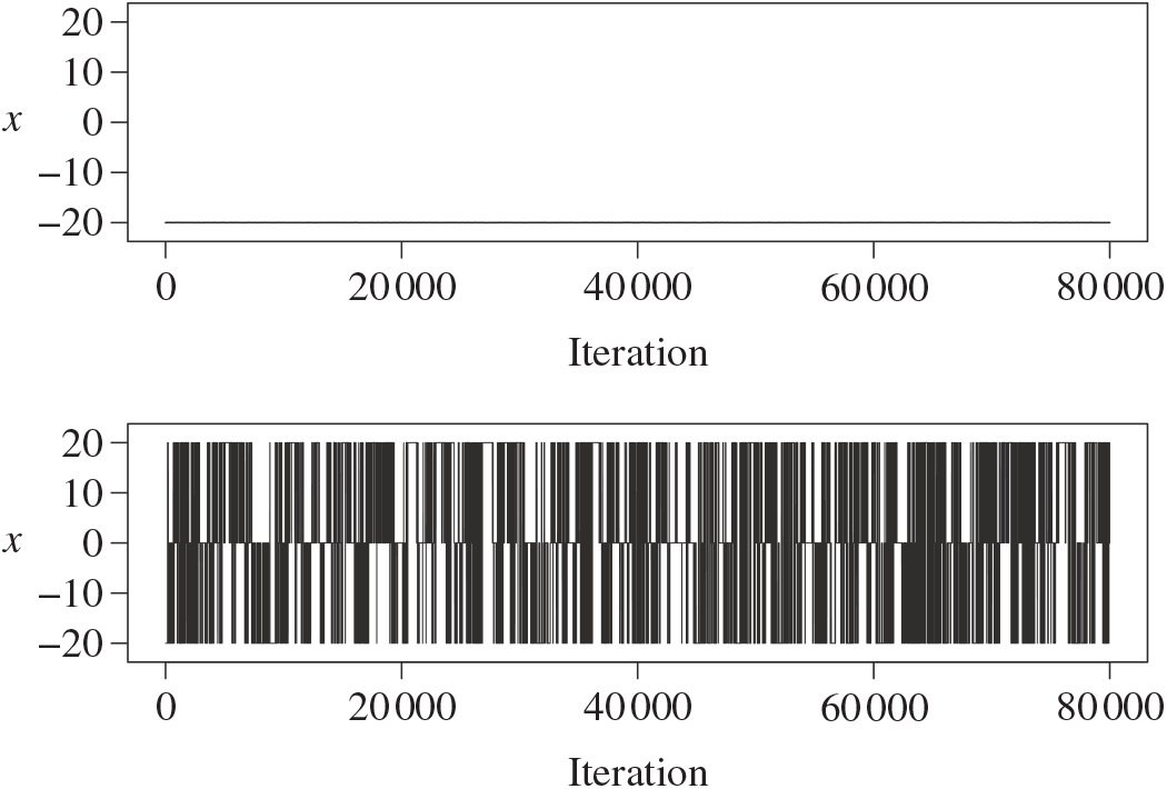
Figure 5: Trace plots of the first component of the twenty dimensional cold state chains for representative runs of the PT (top) and new QuanTA (bottom) schemes. Note the fast inter-modal mixing of the new QuanTA scheme, allowing rapid exploration of the target distribution. In contrast the PT scheme never escapes the initialising mode.
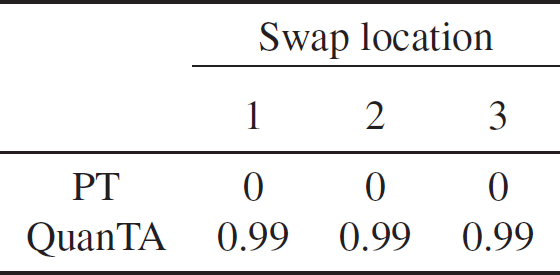
The consecutive swap acceptance rates between the four levels are given in Table 2. Clearly, there is no transfer of mixing information from the hot states to the cold state for the PT algorithm, but there is excellent mixing in the QuanTA scheme.
Table 2: Comparison of the acceptance rates of swap moves for the PT algorithm and QuanTA targeting the twenty-dimensional distribution given in (22) and setup with the ambitious inverse temperature schedule given by
![]() $\{ 1,0.002,0.002^2 ,0.002^3 \}$
.
$\{ 1,0.002,0.002^2 ,0.002^3 \}$
.
The temperature schedule choice that induces a 0.234 swap acceptance rate between consecutive temperature levels for this example using the PT algorithm indicates a geometric schedule with a 0.58 common ratio. This is in stark contrast to the 0.002 ratio that is evidently underambitious for QuanTA. Indeed, to reach the allocated hot state of
![]() $\beta=0.002^3$
then the PT algorithm would need 36 temperature levels in contrast to the 4 that sufficed for QuanTA.
$\beta=0.002^3$
then the PT algorithm would need 36 temperature levels in contrast to the 4 that sufficed for QuanTA.
7.3 Five-dimensional noncanonical example
Leaving the canonical symmetric mode setting, the following example has a five-dimensional Gaussian mixture target with even weight to the modes but with different covariance scaling within each mode. The target distribution is given by
 $$\begin{equation}
\pi(x) \propto \sum_{k=1}^3 w_k \bigg[ \prod_{j=1}^{5}
\phi(x_j\,;\,\mu_k,\sigma_k^2) \bigg].
\label{eqn23}
\end{equation}
$$
In this example,
![]() $(\sigma_1,\sigma_2,\sigma_3)=(0.02,0.01,0.015)$
, the marginal mode centres are given by
$(\sigma_1,\sigma_2,\sigma_3)=(0.02,0.01,0.015)$
, the marginal mode centres are given by
![]() $(\mu_1,\mu_2,\mu_3)=(-20,0,20),$
and all modes are equally weighted with
$(\mu_1,\mu_2,\mu_3)=(-20,0,20),$
and all modes are equally weighted with
![]() $w_1=w_2=w_3$
.
$w_1=w_2=w_3$
.
Although at first glimpse this does not sound like a significantly harder problem, or even far from the canonical setting, the differing modal scalings make this a much more complex example. This is due to the lack of preservation of modal weight through power-based tempering [Reference Woodard, Schmidler and Huber48]. Indeed, Tawn and Roberts [Reference Tawn and Roberts40] and Tawn et al. [Reference Tawn, Roberts and Rosenthal41] presented a novel modification to the auxiliary tempered targets that remain compatible with the QuanTA scheme.
The temperature schedule for this example cannot be a simple geometric schedule as in the previous example due to the scaling indifference between the modes. By using an ambitious geometric schedule, the clustering was very unstable early on and this often led to an inability to establish mode centres for the run. Instead, a mixture of geometric schedules was used with an ambitious spacing for the coldest levels and then a less ambitious spacing for the hotter levels. For the four coldest states, an ambitious geometric schedule with
![]() $0.08$
common ratio was used. A further eight hotter levels were added using a conservative geometric schedule with ratio
$0.08$
common ratio was used. A further eight hotter levels were added using a conservative geometric schedule with ratio
![]() $0.4$
. Hence, the schedule was given by
$0.4$
. Hence, the schedule was given by
For the QuanTA scheme, the transformation moves were used for swap moves between the coldest seven levels and standard swap moves were used otherwise.
In Figure 6 we show two representative trace plots of the target state chain for a run of the PT and QuanTA algorithms. There is a clear improvement in the inter-modal mixing for the QuanTA scheme; albeit far less stark than that in the canonical one-dimensional and twenty-dimensional examples already shown. The run using the standard PT scheme fails to explore the state space. The QuanTA scheme establishes a chain that is able to explore the state space but does appear to have a bit of trouble during burn-in; mixing is good therein.
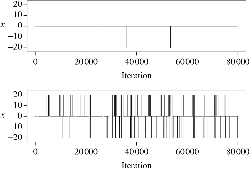
Figure 6: Trace plots of the first component of the five dimensional cold state chains for representative runs of the PT and QuanTA schemes respectively. Note the difference in inter-modal mixing between the QuanTA scheme and the PT scheme which struggles to escape the initialisation mode.
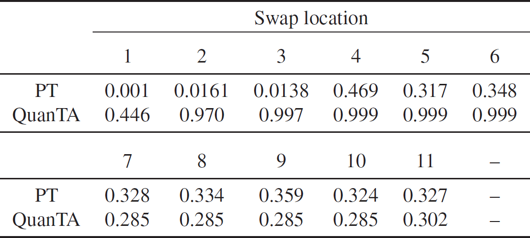
The consecutive swap acceptance rates between the 12 levels are given in Table 3. Clearly, there is very poor mixing through the four coldest states for the PT algorithm. In contrast, the QuanTA scheme has solid swap acceptance rates through the coldest levels but, unlike the previous examples, they are not all close to 1.
Table 3: Comparison of the acceptance rates of swap moves for the PT and new QuanTA algorithms targeting the five-dimensional distribution given in (23) and setup with the ambitious inverse temperature schedule given in (24). Note that, for QuanTA, the reparametrised swap move was only used for swaps in the coldest seven levels.
This example is both positive (showing the improved mixing using the QuanTA scheme on a hard example), but also serves as a warning for the degeneracy of both the PT and new QuanTA schemes when using power-based tempering on a target outside of the canonical symmetric mode setting.
7.4 The computational cost of QuanTA
It is important to analyse the computational cost of QuanTA. To be an effective algorithm, the inferential gains of QuanTA per iteration should not be outweighed by the increase in runtime.
The analysis uses the runs of the one-dimensional and twenty-dimensional examples given above, using both the QuanTA and PT approaches. The algorithms were setup the same as in the ambitious versions of the spacing schedules in each case.
The key idea is to first establish the total runtime, denoted by R, in each case. Typically, one looks to compare the time-standardised effective sample size. In this case it is natural to take the acceptance rate as a direct proxy for the effective sample size. This is due to the fact that the target distributions have symmetric modes with equal weights. Hence, the acceptance rate between consecutive temperature levels dictates the performance of the algorithm, in particular the quality of inter-modal mixing.
To this end, taking the first level temperature swap acceptance rate, denoted by A, the runs are compared using runtime standardised acceptance rates, i.e.
![]() $A/R$
.
$A/R$
.
Note that in both dimensional cases, the output from QuanTA is 100 times larger due to the use of 100 schemes running in parallel. Hence, for a standardised comparison, the time was divided by 100. Therefore, in what follows in this section, when the runtime R of the QuanTA approach is referred to, this means the full runtime divided by 100. The fairness of this is discussed below.
Table 4: Complexity comparisons between QuanTA and PT for the one-dimensional example.
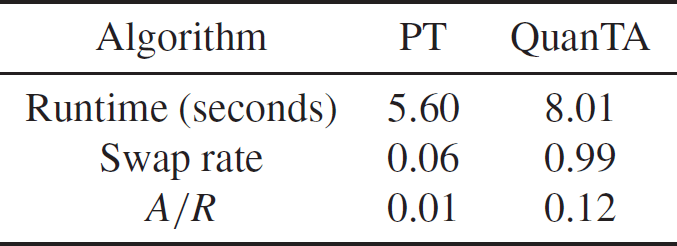
Table 5: Complexity comparisons between QuanTA and PT for the twenty-dimensional example.
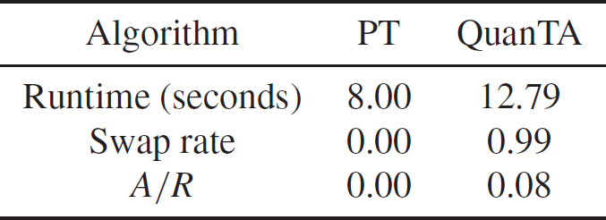
As can be seen in Tables 4 and 5, the QuanTA approach has a longer runtime to generate the same amount of output, as would be expected due to the added cost of clustering. Indeed, it takes approximately 1.5 times longer to generate the ‘same amount of output’. However, the temperature swap move acceptance rates are 16.5 and
![]() $\infty$
times better, respectively, when using the QuanTA approach. Using the acceptance rate as a proxy for the effective sample size, the quantity
$\infty$
times better, respectively, when using the QuanTA approach. Using the acceptance rate as a proxy for the effective sample size, the quantity
![]() $A/R$
is the fundamental value for comparison. In both cases the QuanTA approach shows a significant improvement over the PT approach.
$A/R$
is the fundamental value for comparison. In both cases the QuanTA approach shows a significant improvement over the PT approach.
There are the following issues with the fairness of this comparison.
Standardising the runtime of QuanTA by the number of parallel schemes is not fully fair since it is sharing out the clustering expense between schemes.
The spacings are too ambitious for the PT approach, meaning that the acceptance rates are very low. For a complete analysis, one should run the PT algorithm on its optimal temperature schedule and then use the time-standardised effective sample size from each of the optimised algorithms.
The empirical computational studies are favourable to the QuanTA approach. This is for a couple of examples that are canonical for QuanTA. Outside of this canonical setting the improvements from running QuanTA will be less obvious.
8. Conclusion and further work
The prototype QuanTA approach utilises a noncentred transformation approach to accelerate the transfer of mixing information from the rapidly mixing ‘hot’ state to aid the inter-modal mixing in the target ‘cold’ state. Examples show that this novel algorithm has the potential to dramatically improve the inferential gains, particularly in settings where the modes are similar to a Gaussian in structure.
The accompanying theoretical results that are given in Section 6 show that in a generic non-Gaussian setting the QuanTA approach can still exhibit accelerated mixing through the temperature schedule. Although the inverse temperature spacings are generally still
![]() $\mathcal{O}(d^{-1/2})$
there is a higher-order behaviour exhibited in the mixing for large (i.e. cold) values of the inverse temperature
$\mathcal{O}(d^{-1/2})$
there is a higher-order behaviour exhibited in the mixing for large (i.e. cold) values of the inverse temperature
![]() $\beta$
. This suggests that the QuanTA approach will be powerful for accelerating the mixing through the colder levels of the temperature schedule for a typical smooth target.
$\beta$
. This suggests that the QuanTA approach will be powerful for accelerating the mixing through the colder levels of the temperature schedule for a typical smooth target.
It is clear that there are interesting questions to be addressed and further work needed before QuanTA can be considered practical in a real-data problem. In terms of optimising the computational expense, it has been shown that parallelisation of the PT algorithm can give significant practical gains [Reference VanDerwerken and Schmidler45]; by design, QuanTA is also highly parallelisible. The procedure described in Section 4.1 has huge scope to be parallelised. This requires care since communication costs and synchronisation between parallel collections of the PT schemes could negate the effectiveness of the parallelisation.
A criticism of the current clustering method used is that it requires prior specification of the number of modes K which is likely to be unknown and would need online estimation as part of the clustering process.
An interesting question is whether using extra cold levels (with
![]() $\beta>1$
) along with the weighted clustering would help to aid the stability of the clustering procedure once invariance is reached for the population. Indeed, the mixing at these auxiliary extra cold levels should be very fast due to the QuanTA exhibiting higher-order behaviour in these modes. The other interesting question is regarding the robustness of the method outside of Gaussian modes, e.g. in heavier tailed modes, when the Gaussian approximation to the mode can be poor. Consider the setting of a univariate Laplace distribution and observe that the QuanTA-style transformation never agrees with the true CDF preserving transformation. It would be interesting to search, both empirically and theoretically, for settings where QuanTA fails to outperform the standard PT swap move. Some initial ideas and details of this further work can be found in [Reference Tawn39].
$\beta>1$
) along with the weighted clustering would help to aid the stability of the clustering procedure once invariance is reached for the population. Indeed, the mixing at these auxiliary extra cold levels should be very fast due to the QuanTA exhibiting higher-order behaviour in these modes. The other interesting question is regarding the robustness of the method outside of Gaussian modes, e.g. in heavier tailed modes, when the Gaussian approximation to the mode can be poor. Consider the setting of a univariate Laplace distribution and observe that the QuanTA-style transformation never agrees with the true CDF preserving transformation. It would be interesting to search, both empirically and theoretically, for settings where QuanTA fails to outperform the standard PT swap move. Some initial ideas and details of this further work can be found in [Reference Tawn39].
Appendix A. Proofs
In this section we give the proof details of the results in Section 6.2. Firstly, some key notation is introduced that will be useful throughout this section.
Definition 1
Let
 $ B= \log \bigg( \frac{f_d^{\beta'}(t(x,\beta,\beta^{'}))f_d^{\beta}
(t(\,y,\beta^{'},\beta))}{f_d^{\beta'}(\,y)f_d^{\beta}(x)} \bigg)$
; $h(x) \,{:\!=}\, \log (\,f(x) )$
; $k(x)\,{:\!=}\,(x-\mu)h'(x)$
; and $r(x)\,{:\!=}\,(x-\mu)^2h''(x).$
Then define
 $$\matrix{
{\matrix{
{M(\beta )} \hfill & { = \mathbb {E}{_\beta }(h(z)),} \hfill \cr
} } \cr
{\matrix{
{S(\beta )} \hfill & { = \mathbb {E}{_\beta }(k(z)),} \hfill \cr
} } \cr
{\matrix{
{R(\beta )} \hfill & { = \mathbb {E}{_\beta }(r(z) - k(z)),} \hfill \cr
} } \cr
} $$
where all expectations are with respect to the distribution
![]() ${f^\beta
(x)}/{Z_{\beta}}$
with
${f^\beta
(x)}/{Z_{\beta}}$
with
![]() $Z_{\beta}=\smash{\int f^\beta (z)} {\rm d} z$
.
$Z_{\beta}=\smash{\int f^\beta (z)} {\rm d} z$
.
Proposition 2
Under the notation and assumptions of Theorem 1 and Definition 1, it can be shown that
and
which trivially gives
Proof. The proof of (26) is routine and can be found in [Reference Atchadé, Roberts and Rosenthal1]. The derivation of (27) is less obvious using integration by parts:
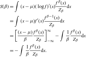 $$\begin{align*}
S(\beta)&=\int (x-\mu) (\log f)'(x) \frac{f^\beta (x)}{Z_{\beta}}{\rm d} x
\\
&= \int (x-\mu) f'(x) \frac{f^{\beta-1} (x)}{Z_{\beta}}{\rm d} x
\\
&= \bigg[ \frac{(x-\mu)}{\beta} \frac{f^{\beta} (x)}{Z_{\beta}}
\bigg]_{-\infty}^{\infty}-\int \frac{1}{\beta} \frac{f^{\beta}
(x)}{Z_{\beta}}{\rm d} x
\\
&= -\int \frac{1}{\beta} \frac{f^{\beta} (x)}{Z_{\beta}}{\rm d} x.
\tag*{\qedhere}
\end{align*}
$$
A.1 Proofs Proof of Theorem 1
In this section we derive three key results that are specific to deriving the result in Theorem 1. Lemma 1 will establish a Taylor-expanded form of the log acceptance ratio of a temperature swap move that will prove to be asymptotically useful. Lemma 2 will then establish the limiting Gaussianity of this logged acceptance ratio and, finally, Lemma 3 completes the proof of Theorem 1 by establishing the optimal spacings and associated optimal acceptance rates required.
Lemma 1
(QuanTA log-acceptance ratio.) Under the notation and assumptions of Theorem 1 and Definition 1,
 $$\begin{align*}
B &= \epsilon\bigg[\sum_{i=1}^d h(x_i)- h(\,y_i)+\frac{1}{2} (
k(\,y_i)-k(x_i))\bigg]\nonumber
\\
& +\frac{\epsilon^2}{8\beta} \bigg[\sum_{i=1}^d
r(x_i)-k(x_i)+r(\,y_i)-k(\,y_i)\bigg]+(T_x +T_y),
\end{align*}
$$
where both
![]() $T_x\rightarrow 0$
and
$T_x\rightarrow 0$
and
![]() $T_y\rightarrow 0$
in probability as
$T_y\rightarrow 0$
in probability as
![]() $d\rightarrow\infty.$
$d\rightarrow\infty.$
Proof. By taking logarithms, it is immediate that
 $$\eqalign{B &= \sum_{i=1}^d [\beta' h (t(x_i,\beta,\beta^{'})) - \beta h(x_i)]+
\sum_{i=1}^d[\beta h(t(\,y_i,\beta^{'},\beta)) -\beta' h (\,y_i) ] \cr &= :\,H_\beta^{\beta'} ({{\bf x}}) +H_{\beta'}^{\beta} ({{\bf y}}).}$$
With the aim being to derive the asymptotic behaviour of the log-acceptance ratio, the next step is to use Taylor expansions (in
![]() $\epsilon$
) to appropriate order so that the asymptotic behaviour of B can be understood.
$\epsilon$
) to appropriate order so that the asymptotic behaviour of B can be understood.
For notational convenience, we
make $h(t(x,\beta,\beta^{'}))$
explicitly dependent on $\epsilon$
:
  \[
\alpha_x(\epsilon)\,{:\!=}\, h(t(x,\beta,\beta^{'}))= \log \bigg[ f \bigg(
\bigg(\frac{\beta}{\beta+\epsilon} \bigg)^{1/2} (x-\mu) +\mu\bigg)
\bigg];
\]
define
 \[
d_x(\epsilon)\,{:\!=}\, \bigg(\frac{\beta}{\beta+\epsilon} \bigg)^{1/2} (x-\mu)
+\mu.
\]
By a Taylor series expansion in
![]() $\epsilon$
, for fixed x, with Taylor remainder correction term denoted by
$\epsilon$
, for fixed x, with Taylor remainder correction term denoted by
![]() $\xi_x$
such that
$\xi_x$
such that
![]() $0<\xi_x<\epsilon$
,
$0<\xi_x<\epsilon$
,
where
 $$\begin{align}
\alpha_x''(\epsilon)&=
\frac{(x-\mu)^2}{4}\frac{\beta}{(\beta+\epsilon)^{3}}(\log
f)''(d_x(\epsilon)) \nonumber
\\
& +\frac{3(x-\mu)}{4}\frac{\beta^{1/2}}{(\beta+\epsilon)^{5/2}}(\log
f)'(d_x(\epsilon)),\label{eqn34}\end{align}
$$
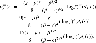 $$\begin{align}
\alpha_x'''(\epsilon)&=
-\frac{(x-\mu)^3}{8}\frac{\beta^{3/2}}{(\beta+\epsilon)^{9/2}}(\log
f)'''(d_x(\epsilon)) \nonumber
\\
& -\frac{9(x-\mu)^2}{8}\frac{\beta}{(\beta+\epsilon)^{4}}(\log
f)''(d_x(\epsilon)) \nonumber
\\
& -\frac{15(x-\mu)}{8}\frac{\beta^{1/2}}{(\beta+\epsilon)^{7/2}}
(\log f)'(d_x(\epsilon)).
\label{eqn35}\end{align}
$$
As a preview to the later stages of this proof, the terms up to second order in
![]() $\epsilon$
dictate the asymptotic distribution of B. However, to show that the higher-order terms ‘disappear’ in the limit as
$\epsilon$
dictate the asymptotic distribution of B. However, to show that the higher-order terms ‘disappear’ in the limit as
![]() $\epsilon
\rightarrow 0,$
a careful analysis is required. Thus, the next step is to establish that, under the assumptions made above, the higher-order terms converge to 0 in probability.
$\epsilon
\rightarrow 0,$
a careful analysis is required. Thus, the next step is to establish that, under the assumptions made above, the higher-order terms converge to 0 in probability.
To this end, a careful analysis of
![]() $\alpha_x'''({\cdot})$
is undertaken. Firstly, it will be shown that
$\alpha_x'''({\cdot})$
is undertaken. Firstly, it will be shown that
![]() $|\mathbb{E}_\beta[\alpha_x'''(\xi_x)] |$
is bounded; then application of Markov’s inequality will establish that the higher-order terms converge to 0 in probability as
$|\mathbb{E}_\beta[\alpha_x'''(\xi_x)] |$
is bounded; then application of Markov’s inequality will establish that the higher-order terms converge to 0 in probability as
![]() $d \rightarrow
\infty$
. Define
$d \rightarrow
\infty$
. Define
so that
which has the property that
![]() $\eta_\epsilon\rightarrow 0$
as
$\eta_\epsilon\rightarrow 0$
as
![]() $d\rightarrow
\infty$
and
$d\rightarrow
\infty$
and
![]() $|\eta_\epsilon| \le 1$
.
$|\eta_\epsilon| \le 1$
.
Then, with Taylor remainder correction terms denoted by
![]() $\xi^\epsilon_1,\xi^\epsilon_2,$
and
$\xi^\epsilon_1,\xi^\epsilon_2,$
and
![]() $\xi^\epsilon_3$
such that
$\xi^\epsilon_3$
such that
![]() $0<|\xi^\epsilon_k-x|<| d_x(\epsilon) -x |,$
$0<|\xi^\epsilon_k-x|<| d_x(\epsilon) -x |,$
 $$\begin{align}
(\log f)'(d_x(\epsilon)) &= (\log f)'(x)+ \eta_\epsilon (x-\mu)(\log
f)''(x) +\frac{ {\eta_\epsilon}^2(x-\mu)^2}{2}(\log f)'''(x) \nonumber
\\
& + \frac{ {\eta_\epsilon}^3(x-\mu)^3}{6}(\log
f)''''(\xi^\epsilon_1),\label{eqn36}\end{align}
$$
Recall the assumptions (14) and (15). Substituting (32), (33), and (34) into (31), evaluating the expectation with respect to
![]() $X\sim f^\beta,$
and, for convenience, denoting
$X\sim f^\beta,$
and, for convenience, denoting
![]() $|x-\mu|$
by S, then there exists
$|x-\mu|$
by S, then there exists
![]() $C \in \mathbb{R}_+$
such that
$C \in \mathbb{R}_+$
such that
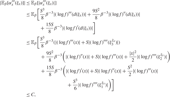 $$\matrix{
{\matrix{
{| \mathbb {E}{_\beta }[{\alpha _{x'''}}({\xi _x})]|} \hfill & { \le {_\beta }[|{\alpha _{x'''}}({\xi _x})|]{\rm{ \backslash nonumber}}} \hfill \cr
{} \hfill & { \le \mathbb {E}{_\beta }[{{{S^3}} \over 8}{\beta ^{ - 3}}|{{(\log f)}^{\prime \prime \prime }}(d({\xi _x}))| + {{9{S^2}} \over 8}{\beta ^{ - 3}}|{{(\log f)}^{\prime \prime }}(d({\xi _x}))|{\rm{\backslash nonumber}}} \hfill \cr
{} \hfill & { + {{15S} \over 8}{\beta ^{ - 3}}|{{(\log f)}^\prime }(d({\xi _x}))|]{\rm{n\backslash nonumber}}} \hfill \cr
{} \hfill & { \le \mathbb {E}{_\beta }[{{{S^3}} \over 8}{\beta ^{ - 3}}(|(\log f)'''(x)| + S|{{(\log f)}^{\prime \prime \prime }}^\prime (\xi _3^{{\xi _x}})|){\rm{ \backslash nonumber}}} \hfill \cr
{} \hfill & { + {{9{S^2}} \over 8}{\beta ^{ - 3}}(|{{(\log f)}^{\prime \prime }}(x)| + S|{{(\log f)}^{\prime \prime \prime }}(x)| + {{|x{|^2}} \over 2}|{{(\log f)}^{\prime \prime \prime }}^\prime (\xi _2^{{\xi _x}})|){\rm{\backslash nonumber}}} \hfill \cr
{} \hfill & { + {{15S} \over 8}{\beta ^{ - 3}}(|{{(\log f)}^\prime }(x)| + S|{{(\log f)}^{\prime \prime }}(x)| + {{{S^2}} \over 2}|{{(\log f)}^{\prime \prime \prime }}(x)|{\rm{\backslash nonumber}}} \hfill \cr \hfill & { + {{{S^3}} \over 6}|{{(\log f)}^{\prime \prime \prime }}^\prime (\xi _1^{{\xi _x}})|)]} \hfill \cr } } \cr
{ \le C,} \cr} $$
where the first three inequalities are from the direct application of the triangle inequality (with the second also using the boundedness of
![]() $\eta_\epsilon$
); whereas the final inequality arises from both the finiteness of expectations of the terms involving derivatives of order three or below (this is due to the regularly varying tails of
$\eta_\epsilon$
); whereas the final inequality arises from both the finiteness of expectations of the terms involving derivatives of order three or below (this is due to the regularly varying tails of
![]() $\log
(\,f({\cdot}))$
) and the assumption that
$\log
(\,f({\cdot}))$
) and the assumption that
![]() $|(\log f)''''({\cdot})|{<}M$
.
$|(\log f)''''({\cdot})|{<}M$
.
Using (28), with substitution of terms from (29), (30), and (31),
![]() $\smash{H_\beta^{\beta'} ({{\bf x}})}$
can be expressed as
$\smash{H_\beta^{\beta'} ({{\bf x}})}$
can be expressed as
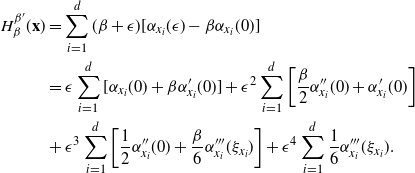 $$\begin{align*}
H_\beta^{\beta'} ({{\bf x}}) &= \sum_{i=1}^d(\beta+\epsilon) [
\alpha_{x_i}(\epsilon) - \beta \alpha_{x_i}(0) ] \nonumber
\\
&=\epsilon \sum_{i=1}^d [\alpha_{x_i}(0)+\beta \alpha_{x_i}'(0)] +
\epsilon^2 \sum_{i=1}^d \bigg[\frac{\beta}{2}\alpha_{x_i}''(0)+
\alpha_{x_i}'(0)\bigg]\nonumber
\\
& +\epsilon^3 \sum_{i=1}^d
\bigg[\frac{1}{2}\alpha_{x_i}''(0)+\frac{\beta}{6}
\alpha_{x_i}'''(\xi_{x_i})\bigg] + \epsilon^4 \sum_{i=1}^d \frac{1}{6}
\alpha_{x_i}'''(\xi_{x_i}).
\end{align*}
$$
By (35) and using the i.i.d. nature of the
![]() $x_i$
and Markov’s inequality, for all
$x_i$
and Markov’s inequality, for all
![]() $\delta>0$
,
$\delta>0$
,
 $$\begin{align*}
\delta \mathbb{P}\bigg( \bigg| \epsilon^3 \sum_{i=1}^d
\bigg[\frac{1}{2}\alpha_{x_i}''(0)
+\frac{\beta}{6}\alpha_{x_i}'''(\xi_{x_i})\bigg] \bigg|>\delta \bigg)
&<\mathbb{E}\bigg( \bigg| \frac{\ell^3}{d^{3/2}} \sum_{i=1}^d
\bigg[\frac{1}{2}\alpha_{x_i}''(0)+\frac{\beta}{6}
\alpha_{x_i}'''(\xi_{x_i})\bigg] \bigg| \bigg) \nonumber
\\
&\le \frac{\ell^3}{d^{1/2}}\bigg[ \frac{1}{2}\mathbb{E}(
|\alpha_{x_i}''(0)| )+ \frac{\beta}{6}C\bigg]
\\
&\rightarrow 0 \quad\text{as } d\rightarrow \infty.
\end{align*}
$$
Thus,
 \[
\epsilon^3 \sum_{i=1}^d \bigg[\frac{1}{2}\alpha_{x_i}''(0)+
\frac{\beta}{6}\alpha_{x_i}'''(\xi_{x_i})\bigg]\rightarrow 0
\quad\text{in probability as } d\rightarrow \infty.
\]
By identical methodology, as
![]() $d\rightarrow \infty,$
$d\rightarrow \infty,$
 $$
\epsilon^4 \sum_{i=1}^d \frac{1}{6} \alpha_{x_i}'''(\xi_{x_i})
\rightarrow 0 \quad\text{in probability}.$$
Consequently,
 $$H_\beta ^{\beta '}({\bf{x}}){\rm{ }} = [\sum\limits_{i = 1}^d h ({x_i}) - {1 \over 2}({x_i} - \mu )h'({x_i})]{\rm{ }} + {{{^2}} \over {8\beta }}[\sum\limits_{i = 1}^d {{{({x_i} - \mu )}^2}} h''({x_i}) - ({x_i} - \mu )h'({x_i})] + {T_x},$$
where
 \[
T_x = \epsilon^3 \sum_{i=1}^d \bigg[\frac{1}{2}\alpha_{x_i}''(0)+
\frac{\beta}{6}\alpha_{x_i}'''(\xi_{x_i})\bigg] + \epsilon^4 \sum_{i=1}^d
\frac{1}{6} \alpha_{x_i}'''(\xi_{x_i}),
\]
with
![]() $T_x \rightarrow 0$
in probability as
$T_x \rightarrow 0$
in probability as
![]() $d\rightarrow \infty$
.
$d\rightarrow \infty$
.
Now denoting
![]() $h(t(\,y,\beta^{'},\beta))$
as
$h(t(\,y,\beta^{'},\beta))$
as
the Taylor series expansion in
![]() $\epsilon$
, for a fixed y, with Taylor truncation term denoted by
$\epsilon$
, for a fixed y, with Taylor truncation term denoted by
![]() $\xi_y$
such that
$\xi_y$
such that
![]() $0<\xi_y<\epsilon$
is given by
$0<\xi_y<\epsilon$
is given by
By identical methodology to the above calculation in (35) for
![]() $\alpha_x({\cdot})$
, it can be shown that there exists
$\alpha_x({\cdot})$
, it can be shown that there exists
![]() $C_y\in \mathbb{R}_+$
such that
$C_y\in \mathbb{R}_+$
such that
Hence, using exactly the same methodology as for the
![]() $x_i$
above,
$x_i$
above,
 $$H_{\beta '}^\beta ({\bf{y}}){\rm{ }} = - [\sum\limits_{i = 1}^d h ({\mkern 1mu} {y_i}) - {1 \over 2}({\mkern 1mu} {y_i} - \mu )h'({\mkern 1mu} {y_i})]{\rm{ }} + {{{^2}} \over {8\beta }}[\sum\limits_{i = 1}^d {{{({\mkern 1mu} {y_i} - \mu )}^2}} h''({\mkern 1mu} {y_i}) - ({\mkern 1mu} {y_i} - \mu )h'({\mkern 1mu} {y_i})] + {T_y},$$
where
![]() $T_y \rightarrow 0$
in probability as
$T_y \rightarrow 0$
in probability as
![]() $d\rightarrow \infty$
.
$d\rightarrow \infty$
.
Using the notation from Definition 1, the desired form of B in Lemma 1 is reached.
Lemma 2
(Asymptotic Gaussianity of the log-acceptance ratio for QuanTA.) Under the notation and assumptions of Theorem 1 and Definition 1, B is asymptotically Gaussian of the form
![]() $B\dot{\sim} N({-\sigma^2},{2},\sigma^2),$
where
$B\dot{\sim} N({-\sigma^2},{2},\sigma^2),$
where
Proof. Recall the form of B from Lemma 1. Then, making the dimensionality dependence explicit, write
![]() $B=W(d)+(T_x+T_y),$
where
$B=W(d)+(T_x+T_y),$
where
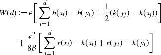 $$\begin{align}
W(d) &\,{:\!=}\, \epsilon\bigg[\sum_{i=1}^d h(x_i)- h(\,y_i)+\frac{1}{2} (
k(\,y_j)-k(x_j))\bigg]\nonumber
\\
& +\frac{\epsilon^2}{8\beta} \bigg[\sum_{i=1}^d
r(x_i)-k(x_i)+r(\,y_i)-k(\,y_i)\bigg] \nonumber
\end{align}
$$
and
![]() $({T_x} + {T_y}) \to 0$
in probability as
$({T_x} + {T_y}) \to 0$
in probability as
![]() $d \rightarrow \infty$
. Hence, if it can be shown that W(d) converges in distribution to a Gaussian of the form
$d \rightarrow \infty$
. Hence, if it can be shown that W(d) converges in distribution to a Gaussian of the form
![]() $N(-c, 2c)$
then by Slutsky’s theorem we can conclude that B converges in distribution to the same Gaussian as the W.
$N(-c, 2c)$
then by Slutsky’s theorem we can conclude that B converges in distribution to the same Gaussian as the W.
To this end, the asymptotic Gaussianity of W(d) is established. First note that, due to the i.i.d. nature of the
![]() $x_i$
and
$x_i$
and
![]() $y_i$
respectively, by the standard central limit theorem (see, e.g. [Reference Durrett6]) for a sum of i.i.d. variables, asymptotic Gaussianity is immediate, where
$y_i$
respectively, by the standard central limit theorem (see, e.g. [Reference Durrett6]) for a sum of i.i.d. variables, asymptotic Gaussianity is immediate, where
and
To this end, the terms
![]() $\mathbb{E}[W(d)]$
and
$\mathbb{E}[W(d)]$
and
![]() ${\rm var}[W(d)]$
are computed. We obtain
${\rm var}[W(d)]$
are computed. We obtain
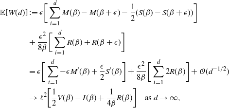 $$\begin{align*}
\mathbb{E}[W(d)] &\,{:\!=}\, \epsilon\bigg[\sum_{i=1}^d
M(\beta)-M(\beta+\epsilon)
-\frac{1}{2}(S(\beta)-S(\beta+\epsilon))\bigg]\nonumber
\\
& +\frac{\epsilon^2}{8\beta} \bigg[\sum_{i=1}^d
R(\beta)+R(\beta+\epsilon)\bigg] \nonumber
\\
&= \epsilon\bigg[\sum_{i=1}^d -\epsilon
M'(\beta)+\frac{\epsilon}{2}S'(\beta)\bigg] +\frac{\epsilon^2}{8\beta}
\bigg[\sum_{i=1}^d 2R(\beta)\bigg] +\mathcal{O}(d^{-1/2})\nonumber
\\
&\rightarrow \ell^2\bigg[\frac{1}{2} V(\beta)
-I(\beta)+\frac{1}{4\beta}R(\beta)\bigg] \quad\mbox{as } d \rightarrow
\infty, \nonumber
\end{align*}
$$
where the final line utilises the results in Proposition 2. Similarly,
Hence, by Slutsky’s theorem, B is asymptotically Gaussian such that
However, this does not obviously have the form required with
![]() $B\dot{\sim}
N({-\sigma^2}/{2},\sigma^2)$
for some
$B\dot{\sim}
N({-\sigma^2}/{2},\sigma^2)$
for some
![]() $\sigma^2$
. This form is verified with the following proposition, which completes the proof of Lemma 2.
$\sigma^2$
. This form is verified with the following proposition, which completes the proof of Lemma 2.
Proposition 3
Under the notation and assumptions of Theorem 1 and Definition 1,
Proof. From (36), let
and
Then, by using the standard properties of variance, it is routine to show that
Consequently, equating the terms on the right-hand side of (38) and (39) shows that if the following can be shown to hold then the required identity in (37) is validated:
The left-hand side (LHS) and right-hand side (RHS) of (40) will be considered separately. The following integration by parts is well defined due to the assumption that
![]() $-\log
(\,f({\cdot}))$
has regularly varying tails. Starting with the RHS and recalling that, from (27),
$-\log
(\,f({\cdot}))$
has regularly varying tails. Starting with the RHS and recalling that, from (27),
![]() $\mathbb{E}_{\beta}(k(x))=-1/\beta$
,
$\mathbb{E}_{\beta}(k(x))=-1/\beta$
,
 $$\begin{align*}
-\frac{1}{4} {\rm var}_{\beta}(k(x)) + \frac{1}{2}V(\beta)&= -\frac{1}{4}
[\mathbb{E}_{\beta}(k(x)^2)-\mathbb{E}_{\beta}(k(x))^2] +
\frac{1}{2\beta^2}
\\
&= -\frac{1}{4} \mathbb{E}_{\beta}(k(x)^2)+ \frac{3}{4\beta^2}.
\end{align*}
$$
Then, noting that
![]() $(\log\ f)'(x)\ f^\beta(x)=f'(x)\ f^{\beta-1}(x)$
, and using integration by parts (by first integrating
$(\log\ f)'(x)\ f^\beta(x)=f'(x)\ f^{\beta-1}(x)$
, and using integration by parts (by first integrating
![]() $f'(x)\ f^{\beta-1}(x)$
),
$f'(x)\ f^{\beta-1}(x)$
),
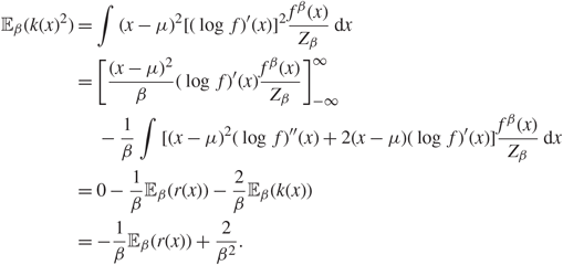 $$\begin{align}
\mathbb{E}_{\beta}(k(x)^2)&=\int (x-\mu)^2 [(\log\ f)'(x)]^2
\frac{f^{\beta}(x)}{Z_{\beta}} {\rm d} x \nonumber
\\
&=\bigg[ \frac{(x-\mu)^2}{\beta} (\log\ f)'(x)\frac{f^{\beta}
(x)}{Z_{\beta}} \bigg]_{-\infty}^{\infty}\nonumber
\\
&-\frac{1}{\beta} \int [(x-\mu)^2 (\log\ f)''(x)+2(x-\mu) (\log\
f)'(x)]\frac{f^{\beta} (x)}{Z_{\beta}}{\rm d} x \nonumber
\\
&= 0-\frac{1}{\beta}\mathbb{E}_{\beta}(r(x))-\frac{2}{\beta}
\mathbb{E}_{\beta}(k(x)) &= -\frac{1}{\beta}\mathbb{E}_{\beta}(r(x))+\frac{2}{\beta^2}.
\label{eqn47}\end{align}
$$
Collating the above in (40) and (41), we obtain
where the final equality simply comes from the definition of
![]() $R(\beta)$
from (25).
$R(\beta)$
from (25).
Lemma 3
(Optimisation of the
![]() ${\rm ESJD}_\beta$
) Under the notation and assumptions of Theorem 1 and Definition 1, the
${\rm ESJD}_\beta$
) Under the notation and assumptions of Theorem 1 and Definition 1, the
![]() ${\rm ESJD}_{\beta}$
is maximised when
${\rm ESJD}_{\beta}$
is maximised when
![]() $\ell$
is chosen to maximise
$\ell$
is chosen to maximise
Furthermore, for the optimal
![]() $\ell,$
the corresponding swap move acceptance rate induced between two consecutive temperatures is given by 0.234 (to three significant figures).
$\ell,$
the corresponding swap move acceptance rate induced between two consecutive temperatures is given by 0.234 (to three significant figures).
Proof. Let
![]() $\smash{\phi_{(m,\sigma^2)}}$
denote the density function of a Gaussian with mean m and variance
$\smash{\phi_{(m,\sigma^2)}}$
denote the density function of a Gaussian with mean m and variance
![]() $\sigma^2,$
and suppose that
$\sigma^2,$
and suppose that
![]() $G\sim
N(-{\sigma^2}/{2},\sigma^2).$
Then a routine calculation (which can be found in, e.g. [Reference Roberts, Gelman and Gilks35]) shows that
$G\sim
N(-{\sigma^2}/{2},\sigma^2).$
Then a routine calculation (which can be found in, e.g. [Reference Roberts, Gelman and Gilks35]) shows that
Using the result in (42) and Lemma 2, in the limit as
![]() $d \rightarrow \infty,$
$d \rightarrow \infty,$
Substituting
and then maximising with respect to u attains an optimising value
![]() $u^*$
that does not depend on
$u^*$
that does not depend on
Recalling the form of the
![]() ${\rm ESJD}_\beta$
from (17), it is clear that the associated acceptance rate, denoted
${\rm ESJD}_\beta$
from (17), it is clear that the associated acceptance rate, denoted
![]() $({\rm
ACC}_\beta)$
, induced by choosing any value of u is
$({\rm
ACC}_\beta)$
, induced by choosing any value of u is
which, as established above, in the limit as
![]() $d \rightarrow \infty$
is asymptotically given by
$d \rightarrow \infty$
is asymptotically given by
Now it can be shown numerically that the optimising value
![]() $u^*$
induces
$u^*$
induces
A.2 Proof of Theorem 2
Note that in Theorem 2 the conditions on
![]() $f({\cdot})$
are inherited from the conditions on
$f({\cdot})$
are inherited from the conditions on
![]() $f({\cdot})$
from Theorem 1. This includes the bounded fourth derivatives of
$f({\cdot})$
from Theorem 1. This includes the bounded fourth derivatives of
![]() $\log(\,f)$
and the existence of eighth moments, i.e.
$\log(\,f)$
and the existence of eighth moments, i.e.
![]() $\mathbb{E}_\beta [ X^8 ]$
, which is due to the assumption of regularly varying tails. These will be assumed for the following lemmata.
$\mathbb{E}_\beta [ X^8 ]$
, which is due to the assumption of regularly varying tails. These will be assumed for the following lemmata.
Lemma 4
Under the notation and assumptions of Theorems 1 and 2 and Definition 1,
where, in general,
![]() $k=\min\{2+\gamma, 5/2 \},$
but if
$k=\min\{2+\gamma, 5/2 \},$
but if
![]() $h'''(0)=0$
then
$h'''(0)=0$
then
![]() $k=\min\{2+\gamma, 3 \}$
.
$k=\min\{2+\gamma, 3 \}$
.
Proof. It has already been established that
![]() $V(\beta)=1/\beta^2$
for all distributions. Also, for a Gaussian density
$V(\beta)=1/\beta^2$
for all distributions. Also, for a Gaussian density
![]() $f({\cdot})$
,
$f({\cdot})$
,
![]() $I(\beta)=1/(2\beta^2)$
. Since
$I(\beta)=1/(2\beta^2)$
. Since
![]() $g_\beta ({\cdot})$
approaches the density of a standard Gaussian,
$g_\beta ({\cdot})$
approaches the density of a standard Gaussian,
![]() $\phi({\cdot})$
, as
$\phi({\cdot})$
, as
![]() $\beta \rightarrow \infty$
, then we expect that
$\beta \rightarrow \infty$
, then we expect that
![]() $I(\beta)$
would approach
$I(\beta)$
would approach
![]() $1/(2\beta^2)$
too. Hence, a rigorous analysis of this convergence needs to be established. Note that
$1/(2\beta^2)$
too. Hence, a rigorous analysis of this convergence needs to be established. Note that
 $$\begin{align}
I(\beta) &= {\rm var}_\beta [h(X)] \nonumber
\\
&= \int (h(x)- \mathbb{E}_\beta [h(X)] )^2 \frac{f^\beta(x)}{Z(\beta)}
{\rm d} x \nonumber
\\
&= \int \bigg(h\bigg(\frac{y}{\sqrt{\beta (-h''(0))}\,}\bigg)-
\mathbb{E}_{g_\beta} \bigg[h\bigg(\frac{y}{\sqrt{\beta
(-h''(0))}\,}\bigg)\bigg] \bigg)^2 g_\beta(\,y) {\rm d} y,
\label{eqn49}\end{align}
$$
using the change of variable,
![]() $X={Y}/{\sqrt{\beta (-h''(0))}}$
. By Taylor expansion of h about the mode point 0 up to fourth order,
$X={Y}/{\sqrt{\beta (-h''(0))}}$
. By Taylor expansion of h about the mode point 0 up to fourth order,
where
![]() $\xi_1({\cdot})$
is the truncation term for the Taylor expansion such that
$\xi_1({\cdot})$
is the truncation term for the Taylor expansion such that
![]() $0<|\xi_1(\,y)| < |{y}/{\sqrt{\beta (-h''(0))}}|$
for all y. Using the Taylor expansion form of h and the assumption of bounded fourth derivatives,
$0<|\xi_1(\,y)| < |{y}/{\sqrt{\beta (-h''(0))}}|$
for all y. Using the Taylor expansion form of h and the assumption of bounded fourth derivatives,
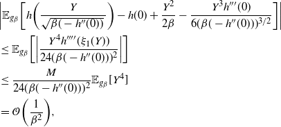 $$\begin{align*}
&\bigg|\mathbb{E}_{g_\beta} \bigg[h\bigg(\frac{Y}{\sqrt{\beta
(-h''(0))}\,}\bigg)-h(0)+\frac{Y^2}{2\beta }-\frac{Y^3 h'''(0)}{6(\beta
(-h''(0)))^{3/2}}\bigg] \bigg|
\\
& \leq \mathbb{E}_{g_\beta} \bigg[\bigg|\frac{Y^4
h''''(\xi_1(Y))}{24(\beta (-h''(0)))^{2}}\bigg|\bigg]
\\
&\leq \frac{M}{24(\beta (-h''(0)))^{2}}\mathbb{E}_{g_\beta} [Y^4 ]
\\
&=\mathcal{O}\bigg( \frac{1}{\beta^2} \bigg),
\end{align*}
$$
where
![]() $\mathbb{E}_{g_\beta} [Y^4 ]<\infty$
due to the assumption on the existence of moments up to the eighth moment. Thus,
$\mathbb{E}_{g_\beta} [Y^4 ]<\infty$
due to the assumption on the existence of moments up to the eighth moment. Thus,
 $$\begin{align*}
\mathbb{E}_{g_\beta} \bigg[h\bigg(\frac{Y}{\sqrt{\beta
(-h''(0))}\,}\bigg)\bigg]&= h(0)-\frac{\mathbb{E}_{g_\beta} [Y^2]
}{2\beta }+\frac{\mathbb{E}_{g_\beta} [Y^3] h'''(0)}{6(\beta
(-h''(0)))^{3/2}}
\\
& + \frac{\mathbb{E}_{g_\beta} [Y^4 h''''(\xi_1(Y))] }{24(\beta
(-h''(0)))^{2}},
\end{align*}
$$
and substituting this into (43), along with the Taylor expansion of h to the fourth order given in (44), gives
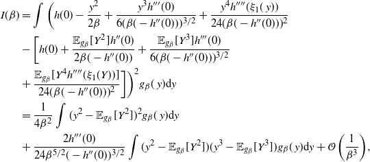 $$\begin{align*}
I(\beta)&= \int \bigg( h(0)-\frac{y^2 }{2\beta }+\frac{y^3 h'''(0)}
{6(\beta (-h''(0)))^{3/2}}+\frac{y^4 h''''(\xi_1(\,y))}{24(\beta
(-h''(0)))^{2}}
\\
& -\bigg[ h(0)+\frac{\mathbb{E}_{g_\beta} [Y^2]
h''(0)}{2\beta (-h''(0))}+\frac{\mathbb{E}_{g_\beta} [Y^3 ]
h'''(0)}{6(\beta (-h''(0)))^{3/2}}
\\
&+ \frac{\mathbb{E}_{g_\beta} [Y^4 h''''(\xi_1(Y))]
}{24(\beta (-h''(0)))^{2}} \bigg] \bigg)^2 g_\beta(\,y){\rm d} y
\\
&= \frac{1}{4\beta^2} \int ( y^2 - \mathbb{E}_{g_\beta} [Y^2] )^2
g_\beta(\,y){\rm d} y
\\
& +\frac{2h'''(0)}{24\beta^{5/2}(-h''(0))^{3/2}} \int ( y^2 -
\mathbb{E}_{g_\beta} [Y^2] )( y^3 - \mathbb{E}_{g_\beta} [Y^3]
)g_\beta(\,y){\rm d} y +\mathcal{O}\bigg( \frac{1}{\beta^3} \bigg),
\end{align*}
$$
which is finite and well defined due to (14) and (15). Consequently, in general,
but in the case that
![]() $h'''(0)=0$
, which indeed holds in the case that f is symmetric about the mode point, then
$h'''(0)=0$
, which indeed holds in the case that f is symmetric about the mode point, then
and so, under the key assumption given in (19),
where, in general,
![]() $k=\min\{2+\gamma, 5/2 \},$
but if
$k=\min\{2+\gamma, 5/2 \},$
but if
![]() $h'''(0)=0$
then
$h'''(0)=0$
then
![]() $k=\min\{2+\gamma, 3 \}$
, and so
$k=\min\{2+\gamma, 3 \}$
, and so
![]() $\smash{\tfrac{1}{2}} V(\beta)
-I(\beta)=\mathcal{O}({1}/{\beta^k})$
.
$\smash{\tfrac{1}{2}} V(\beta)
-I(\beta)=\mathcal{O}({1}/{\beta^k})$
.
Lemma 5
Under the notation and assumptions of Theorems 1 and 2 and Definition 1,
where, in general,
![]() $k= 5/2, $
but if
$k= 5/2, $
but if
![]() $h'''(0)=0$
then
$h'''(0)=0$
then
![]() $k=3$
.
$k=3$
.
Proof. Recall that
 $$\matrix{
{{1 \over {4\beta }}R(\beta ) = {1 \over {4\beta }}{n_\beta }[{X^2}h''(X) - Xh'(X)]} \cr
{\, = {1 \over {4\beta }}{n_{{g_\beta }}}[{{({Y \over {\sqrt {\beta ( - h''(0))} {\mkern 1mu} }})}^2}h''({Y \over {\sqrt {\beta ( - h''(0))} {\mkern 1mu} }})} \cr
{ - {Y \over {\sqrt {\beta ( - h''(0))} {\mkern 1mu} }}h'({Y \over {\sqrt {\beta ( - h''(0))} {\mkern 1mu} }})]} \cr
} $$
Using Taylor’s expansion about the mode at 0,
 $$h'({y \over {\sqrt {\beta ( - h''(0))} {\mkern 1mu} }}){\rm{ }} = h'(0) + {y \over {\sqrt {\beta ( - h''(0))} {\mkern 1mu} }}h''(0) + {{{y^2}} \over {2\beta ( - h''(0))}}h'''(0){\rm{ }} + {{{y^3}} \over {6{\beta ^{3/2}}{{( - h''(0))}^{3/2}}}}h''''({\xi _2}({\mkern 1mu} y)),\% $$
where
![]() $\xi_2({\cdot})$
is the truncation term for the Taylor expansion such that
$\xi_2({\cdot})$
is the truncation term for the Taylor expansion such that
![]() $ 0<|\xi_2(\,y)|< |{y}/{\sqrt{\beta (-h''(0))}\,}|$
for all y. Also,
$ 0<|\xi_2(\,y)|< |{y}/{\sqrt{\beta (-h''(0))}\,}|$
for all y. Also,
where
![]() $\xi_3({\cdot})$
is the truncation term for the Taylor expansion such that
$\xi_3({\cdot})$
is the truncation term for the Taylor expansion such that
![]() $0<|\xi_3(\,y)|< |{y}/{\sqrt{\beta (-h''(0))}}|$
for all y. Hence,
$0<|\xi_3(\,y)|< |{y}/{\sqrt{\beta (-h''(0))}}|$
for all y. Hence,
 $$\begin{align*}
&\frac{y^2}{2\beta(-h''(0))}h'' \bigg(\frac{y}{\sqrt{\beta (-h''(0))}\,}
\bigg)-\frac{y}{\sqrt{\beta (-h''(0))}\,}h' \bigg(\frac{y}{\sqrt{\beta
(-h''(0))}\,}\bigg)
\\
& = \frac{y^3}{2(\beta(-h''(0)))^{3/2}}
h'''(0)+\frac{y^4}{(\beta(-h''(0)))^{2}}\bigg[
\frac{1}{2}h''''(\xi_3(\,y))- \frac{1}{6} h''''(\xi_2(\,y))\bigg].
\end{align*}
$$
Substituting this into the
![]() $R(\beta)/{4\beta }$
term in (45),
$R(\beta)/{4\beta }$
term in (45),
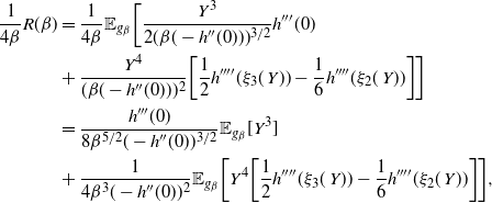 $$\begin{align*}
\frac{1}{4\beta }R(\beta)&= \frac{1}{4\beta }\mathbb{E}_{g_\beta} \bigg[
\frac{Y^3}{2(\beta(-h''(0)))^{3/2}} h'''(0)
\\
&+\frac{Y^4}{(\beta(-h''(0)))^{2}}\bigg[
\frac{1}{2}h''''(\xi_3(\,Y))- \frac{1}{6} h''''(\xi_2(\,Y))\bigg]
\bigg]\nonumber
\\
&= \frac{h'''(0)}{8\beta^{5/2} (-h''(0))^{3/2}}\mathbb{E}_{g_\beta}[ Y^3]
\\
& + \frac{1}{4\beta^{3} (-h''(0))^{2}} \mathbb{E}_{g_\beta} \bigg[
Y^4 \bigg[\frac{1}{2}h''''(\xi_3(\,Y))- \frac{1}{6}
h''''(\xi_2(\,Y))\bigg]\bigg], \nonumber
\end{align*}
$$
where
due to the assumptions of boundedness of the fourth derivatives of
![]() $\log
f(X)$
and the existence of moments. Hence, in general,
$\log
f(X)$
and the existence of moments. Hence, in general,
but in the case that
![]() $h'''({\cdot})=0$
, which is the case when
$h'''({\cdot})=0$
, which is the case when
![]() $f({\cdot})$
is symmetric about the mode point 0,
$f({\cdot})$
is symmetric about the mode point 0,
Consequently,
where, in general,
![]() $k= 5/2$
, but in the case that
$k= 5/2$
, but in the case that
![]() $h'''(0)=0$
then
$h'''(0)=0$
then
![]() $k= 3
$
.
$k= 3
$
.
Acknowledgements
Both authors would like to acknowledge the funding from the EPSRC grants EP/L505110/1 and EP/KO14463/1 that made this work possible. We would also like to thank both Professors Jonathan Tawn (Lancaster) and Jeff Rosenthal (Toronto) for the helpful suggestions and support during the work.


