Nomenclature
- HMV
-
Hypersonic morphing vehicle
- HFV
-
Hypersonic flight vehicle
- ADRC
-
Active disturbance rejection control
- FDO
-
Fixed-time disturbance observer
- AFFDO
-
Adaptive fuzzy fixed-time disturbance observer
- FTC
-
Fixed-time control
1.0 Introduction
One of the strengths of hypersonic morphing vehicles (HMVs) is their adaptation to various flight missions and environments [Reference Bao, Wang and Tang1]. Compared with conventional hypersonic flight vehicles (HFVs), HMVs constantly change their aerodynamic shape to obtain optimal aerodynamic characteristics [Reference Liu, Liang, Han and Yang2, Reference Liu, Deng and Lu3]. Further, the acquired aerodynamic forces and moments are conducive to enhancing flight efficiency and manoeuverability [Reference Liu, Deng and Lu3].
However, it is frustrating that the design procedure of the control system is more difficult after introducing the span morphing technology into HFVs [Reference Liu, Zhang, Cui, Han and Yu4]. The significant changes in aerodynamic characteristics demand strong robustness and adaptation of the control system [Reference Liu, Zhang, Cui, Han and Yu5]. Moreover, the properties, such as the mass distribution, the inertia of moment, and additional moments, vary rapidly, significantly impacting the attitude control. When HMVs perform a flight mission with continuous span morphing, the multisource uncertainties that consist of external disturbances, un-modelled aerodynamics, and aerodynamic perturbation may cause crucial control issues [Reference Ding, Yue, Chen and Si6, Reference Ding, Yue, Chen and Si7]. Therefore, it is necessary to consider the impact of the multisource uncertainties since the control failure may occur in the morphing phase.
The anti-disturbance methods are long-term developed for robustness enhancement [Reference Ren, Jiang and Yang8, Reference Zhang, Hu, Wei and Xu9]. Worldwide researchers propose many disturbance compensation methods, such as active disturbance rejection control (ADRC) and adaptive compensator [Reference Lu10, Reference Wang, Li, Zhou, Zong and Hua11]. Some other researchers take full advantage of robust controllers to passively suppress disturbances. The observers-based method is regarded as an active way to compensate for the disturbance, which is popular in the controller design for HMVs [Reference Wang, Wen, Zhou and Hua12, Reference Chen, Zhu, Wei, Xu and Zhang13]. The commonly used methods are nonlinear disturbance observer and extended state observer [Reference Man and Bai14]. Both disturbance estimation strategies are introduced in the flight control system for disturbance compensation [Reference Zhao, Feng, Cui and Wang15]. Though the conventional nonlinear disturbance observer has achieved fruitful applications, there still exists opportunities to enhance the performance [Reference Liu, Liu, Zhou, Wang, Cheng and Fan16]. The first point is combining the disturbance observer with the fixed/finite-time control method to achieve a fast and high-accuracy anti-disturbance attitude control system [Reference Wu, Wang, Yu, Liu and Wu17]. The other is introducing intelligent control methods, such as a fuzzy logic system, neural network, and iterative learning method, to increase the intelligent level of flight control [Reference Hu, Wang and Yang18, Reference Yu, Jiang, Zhen, Bhatia and Wang19]. Such research motivates us to develop a novel fixed-time disturbance observer (FDO), named adaptive fuzzy fixed-time disturbance observer (AFFDO) [Reference Chen, Huang, Wu and Tu20–Reference Zhao and Yang23].
The most important work is to design a robust controller for attitude angle tracking, which is especially demanded in morphing phases. It is necessary to make deliberate choices, even though a large selection of control methods is available for HFVs [Reference Yu, Li and Zhang24, Reference Ding, Yue, Liu, Dai and Chen25]. The sliding mode control is always adopted to develop robust controllers for hypersonic vehicles because of its robustness. In past decades, the asymptotically stable system theory has always been chosen in sliding mode flight controllers. To enhance the convergence performance, finite/fixed-time stability is developed [Reference Guo, Yang and Guo26]. The fixed-time control (FTC) method stands out because of its outstanding convergence rate and the scalable controller structure [Reference Tang, Zhai and Li27]. Moreover, unlike the finite-time control method, the fixed-time controller forces the closed-loop system to converge in the fixed time, which is related to some controller parameters instead of the initial value of the HMV system [Reference Zhang, Zong, Dou, Tian and Liu28, Reference Ding, Yue, Chen and Si29]. Therefore, combining the sliding mode control and fixed-time control is a wise way to derive a robust controller [Reference Dong, Li and Lv30].
Based on the above discussions, this paper focuses on proposing a fixed-time control technique integrated with the anti-uncertainty technique for the hypersonic morphing vehicle. Strong robustness is demanded to deal with the multisource uncertainties and the rapid aerodynamic characteristics variation in the morphing phase. Therefore, a fixed-time controller combined with an adaptive fuzzy fixed-time disturbance observer is presented for HMVs. Hypersonic flights in morphing phases is adopted to build the test scenario since the aerodynamic changes are significant. The major contributions in this paper are as follows.
-
1) A fixed-time flight control strategy is developed for HMVs. The designed procedure fully utilises the multivariable sliding mode manifold and homogenous system theory. Unlike the traditional fixed-time methods [Reference Wang, Guo, Tang and Qi37], the proposed controllers will lead to a more explicit settling time instead of a complex expression with many parameters. Thus, one can pre-assign the settling time in the controller design.
-
2) An adaptive fuzzy fixed-time disturbance observer is developed. The multisource uncertainty can be exactly estimated. Unlike the super-twisting algorithm-based fixed-time disturbance observer [Reference Wang, Guo, Tang and Qi37], the designed disturbance observer does not require the knowledge of disturbance derivatives. Thus, the application of the AFFDO in actual hypersonic flights with unknown disturbances could be promoted.
-
3) The proposed control design scheme gets rid of the decoupling issue, and the control input is directly obtained instead of traditional inner-loop and outer-loop designs.
-
4) Since the aerodynamic changes are significant, hypersonic flights in the continuous morphing stage are employed to build the simulation case. By using the simulations, the performance will be analysed.
2.0 Preparations and system transformation
2.1 Model of hypersonic morphing vehicle
This section introduces the hypersonic vehicle model with morphing-span wings. The effect of variable span wings is included in the aerodynamics. Meanwhile, all the configurations can be found in [Reference Bao, Wang and Tang1].
2.1.1 Model of hypersonic morphing vehicle
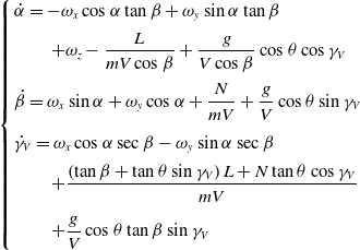
The model of the hypersonic morphing vehicle is given below.
 \begin{align}\left\{ \begin{array}{l}\dot \alpha = - {\omega _x}\cos \alpha \tan \beta + {\omega _y}\sin \alpha \tan \beta \\[5pt] \qquad + {\omega _z} - \dfrac{L}{{mV\cos \beta }} + \dfrac{g}{{V\cos \beta }}\cos \theta \cos {\gamma _V}\\[11pt]\dot \beta = {\omega _x}\sin \alpha + {\omega _y}\cos \alpha + \dfrac{N}{{mV}} + \dfrac{g}{V}\cos \theta \sin {\gamma _V}\\[11pt]{{\dot \gamma }_V} = {\omega _x}\cos \alpha \sec \beta - {\omega _y}\sin \alpha \sec \beta \\[5pt]\qquad + \dfrac{{\left( {\tan \beta + \tan \theta \sin {\gamma _V}} \right)L + N\tan \theta \cos {\gamma _V}}}{{mV}}\\[11pt]\qquad + \dfrac{g}{V}\cos \theta \tan \beta \sin {\gamma _V}\end{array} \right.\end{align}
 \begin{align}\left\{ {\begin{array}{*{20}{c}}{{{\dot \omega }_x} = I_x^{ - 1}\!\left( {{M_x} + {M_{sx}}} \right) + I_x^{ - 1}\!\left( {{I_y} - {I_z}} \right){\omega _y}{\omega _z} - I_x^{ - 1}{{\dot I}_x}{\omega _x}}\\[5pt]{{{\dot \omega }_y} = I_y^{ - 1}\!\left( {{M_y} + {M_{sy}}} \right) + I_z^{ - 1}\!\left( {{I_z} - {I_x}} \right){\omega _z}{\omega _x} - I_y^{ - 1}{{\dot I}_y}{\omega _y}}\\[5pt]{{{\dot \omega }_z} = I_z^{ - 1}\!\left( {{M_z} + {M_{sz}}} \right) + I_z^{ - 1}\!\left( {{I_x} - {I_y}} \right){\omega _x}{\omega _y} - I_z^{ - 1}{{\dot I}_z}{\omega _z}}\end{array}} \right.\end{align}
where
![]() $\alpha ,\beta $
and
$\alpha ,\beta $
and
![]() ${\gamma _V}$
represent the attack angle, sideslip angle and bank angle, respectively.
${\gamma _V}$
represent the attack angle, sideslip angle and bank angle, respectively.
![]() ${\omega _x},{\omega _y}$
and
${\omega _x},{\omega _y}$
and
![]() ${\omega _z}$
indicate the rolling angle rate, yawing angle rate and pitching angle rate, respectively.
${\omega _z}$
indicate the rolling angle rate, yawing angle rate and pitching angle rate, respectively.
![]() $L,D$
and
$L,D$
and
![]() $N$
represent the lift force, the drag force and the lateral force.
$N$
represent the lift force, the drag force and the lateral force.
![]() $V,m$
and
$V,m$
and
![]() $g$
denote the flight velocity, the mass and the gravitational acceleration.
$g$
denote the flight velocity, the mass and the gravitational acceleration.
![]() ${M_x},{M_y}$
and
${M_x},{M_y}$
and
![]() ${M_z}$
stand for the roll, yaw, pitch moment.
${M_z}$
stand for the roll, yaw, pitch moment.
![]() ${M_{sx}},{M_{sy}}$
and
${M_{sx}},{M_{sy}}$
and
![]() ${M_{sz}}$
are the additional moments directly caused by the span variant.
${M_{sz}}$
are the additional moments directly caused by the span variant.
![]() ${I_x},{I_y}$
and
${I_x},{I_y}$
and
![]() ${I_z}$
are roll, pitch and yaw moment of inertia. The forces and moments can be described as follows.
${I_z}$
are roll, pitch and yaw moment of inertia. The forces and moments can be described as follows.
 \begin{align}\left\{ \begin{array}{l}L = q{S_0}{{\bar C}_L}\\[5pt]D = q{S_0}{{\bar C}_D}\\[5pt]N = q{S_0}{{\bar C}_N}\end{array} \right.\quad\end{align}
 \begin{align}\left\{ \begin{array}{l}{M_x} = q{S_0}{L_1}{{\bar m}_x}\\[5pt]{M_y} = q{S_0}{L_1}{{\bar m}_y}\\[5pt]{M_z} = q{S_0}{L_2}{{\bar m}_z}\end{array} \right.\end{align}
where
![]() ${\bar m_x},{\bar m_y}$
and
${\bar m_x},{\bar m_y}$
and
![]() ${\bar m_z}$
represent the equivalent roll, yaw and pitch moment coefficient, respectively.
${\bar m_z}$
represent the equivalent roll, yaw and pitch moment coefficient, respectively.
![]() ${\bar C_L},{\bar C_N}$
and
${\bar C_L},{\bar C_N}$
and
![]() ${\bar C_D}$
denote the equivalent aerodynamic force coefficients.
${\bar C_D}$
denote the equivalent aerodynamic force coefficients.
![]() $q$
is dynamic pressure.
$q$
is dynamic pressure.
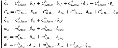
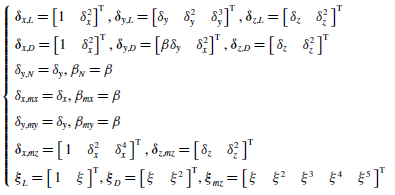
The aerodynamic parameters are listed as
 \begin{align}\left\{ \begin{array}{l}{{\bar C}_i}\!\left( \xi \right) = \dfrac{{S\!\left( \xi \right){C_i}\!\left( \xi \right)}}{{{S_0}}},i = L,D,N\\[13pt]{{\bar m}_i}\!\left( \xi \right) = \dfrac{{S\!\left( \xi \right){m_i}\!\left( \xi \right)}}{{{S_0}}},i = x,y,z\end{array} \right.\end{align}
 \begin{align}\left\{ \begin{array}{l} {{\bar C}_L} = C_{L,Ma,\alpha }^{{\delta _x}} \cdot {{\boldsymbol{\delta }}_{x,L}} + C_{L,Ma,\alpha }^{{\delta _y}} \cdot {{\boldsymbol{\delta }}_{y,L}} + C_{L,Ma,\alpha }^{{\delta _z}} \cdot {{\boldsymbol{\delta }}_{z,L}} + C_{L,Ma,\alpha }^\xi \cdot {{\boldsymbol{\xi }}_L} \\[5pt] {{\bar C}_D} = C_{D,Ma,\alpha }^{{\delta _x}} \cdot {{\boldsymbol{\delta }}_{x,D}} + C_{D,Ma,\alpha }^{{\delta _y}} \cdot {{\boldsymbol{\delta }}_{y,D}} + C_{D,Ma,\alpha }^{{\delta _z}} \cdot {{\boldsymbol{\delta }}_{z,D}} + C_{D,Ma,\alpha }^\xi \cdot {{\boldsymbol{\xi }}_D} \\[5pt] {{\bar C}_N} = C_{N,Ma,\alpha }^\beta \cdot {\beta _N} + C_{N,Ma,\alpha }^{{\delta _y}} \cdot {\delta _{y,N}} \\[5pt] {{\bar m}_x} = m_{x,Ma,\alpha }^\beta \cdot {\beta _{mx}} + m_{x,Ma,\alpha }^{{\delta _x}} \cdot {\delta _{x,mx}} \\[5pt] {{\bar m}_y} = m_{y,Ma,\alpha }^\beta \cdot {\beta _{my}} + m_{y,Ma,\alpha }^{{\delta _y}} \cdot {\delta _{y,my}} \\[5pt] {{\bar m}_z} = m_{z,Ma,\alpha }^{{\delta _x}} \cdot {{\boldsymbol{\delta }}_{x,mz}} + m_{z,Ma,\alpha }^{{\delta _z}} \cdot {{\boldsymbol{\delta }}_{z,mz}} + m_{z,Ma,\alpha }^\xi \cdot {{\boldsymbol{\xi }}_{mz}} \end{array} \right.\end{align}
 \begin{align}\left\{ \begin{array}{l}{\boldsymbol{\delta }}_{x,L} = \left[ {1 \quad \delta _x^2} \right]^{\rm T},{\boldsymbol{\delta }}_{y,L} = \left[ {\delta _y\quad \delta _y^2\quad \delta _y^3} \right]^{\rm T},{\boldsymbol{\delta }}_{z,L} = \left[ {\begin{array}{*{20}{c}}{\delta _z}\quad {\delta _z^2}\end{array}} \right]^{\rm T}\\[5pt]{\boldsymbol{\delta }}_{x,D} = \left[ {1\quad \delta _x^2} \right]^{\rm T},{\boldsymbol{\delta }}_{y,D} = \left[ {\beta \delta _y\quad \delta _x^2} \right]^{\rm T},{\boldsymbol{\delta }}_{z,D} = \left[ {\begin{array}{*{20}{c}}{\delta _z}\quad {\delta _z^2}\end{array}} \right]^{\rm T}\\[5pt]\delta _{y,N} = \delta _y,{\beta _N} = \beta \\[5pt]\delta _{x,mx} = \delta _x,{\beta _{mx}} = \beta \\[5pt]\delta _{y,my} = \delta _y,{\beta _{my}} = \beta \\[5pt]{\boldsymbol{\delta }}_{x,mz} = \left[ {\begin{array}{*{20}{c}}1\quad {\delta _x^2}\quad {\delta _x^4}\end{array}} \right]^{\rm T},{\boldsymbol{\delta }}_{z,mz} = \left[ {\begin{array}{*{20}{c}}{\delta _z}\quad {\delta _z^2}\end{array}} \right]^{\rm T}\\[5pt]{{\boldsymbol{\xi }}_L} = {\left[ {\begin{array}{*{20}{c}}1\quad \xi \end{array}} \right]^{\rm T}},{{\boldsymbol{\xi }}_D} = {\left[ {\begin{array}{*{20}{c}}\xi\quad {{\xi ^2}}\end{array}} \right]^{\rm T}},{{\boldsymbol{\xi }}_{mz}} = {\left[ {\begin{array}{*{20}{c}}\xi\quad {{\xi ^2}}\quad {{\xi ^3}}\quad {{\xi ^4}}\quad {{\xi ^5}}\end{array}} \right]^{\rm T}}\end{array} \right.\end{align}
where
![]() $\xi $
and
$\xi $
and
![]() $Ma$
denote the span morphing rate and Mach.
$Ma$
denote the span morphing rate and Mach.
![]() ${\delta _x},{\delta _y}$
and
${\delta _x},{\delta _y}$
and
![]() ${\delta _z}$
represent the roll elevator deflection, yaw elevator deflection and pitch elevator deflection.
${\delta _z}$
represent the roll elevator deflection, yaw elevator deflection and pitch elevator deflection.
In this paper, the aerodynamic forces and moments are simplified as
 \begin{align}\left\{ \begin{array}{l}L = q{S_0}\bar C_L^{\boldsymbol{\alpha }}{\boldsymbol{\alpha }} + {\Delta _L}\\[9pt]N = q{S_0}\bar C_N^\beta + {\Delta _N}\end{array} \right.\end{align}
 \begin{align}\left\{ \begin{array}{l}{M_x} = q{S_0}{L_1}\!\left( {\bar m_x^\beta {\beta _{mx}} + \bar m_x^{{\delta _x}}{\delta _x}} \right) + {\Delta _{{M_x}}}\\[9pt]{M_y} = q{S_0}{L_1}\!\left( {\bar m_y^\beta {\beta _{mx}} + c{\delta _y}} \right) + {\Delta _{{M_y}}}\\[9pt]{M_z} = q{S_0}{L_2}{{\bar m}_z}\!\left( {\bar{\boldsymbol{m}}_z^{\boldsymbol{\alpha }}{\boldsymbol{\alpha }} + \bar m_z^{{\delta _z}}{\delta _z}} \right) + {\Delta _{{M_z}}}\end{array} \right.\end{align}
where
![]() ${\boldsymbol{\alpha }} = {[\begin{array}{*{20}{c}}1\quad \alpha\quad {{\alpha ^3}}\end{array}]^{\rm T}}$
.
${\boldsymbol{\alpha }} = {[\begin{array}{*{20}{c}}1\quad \alpha\quad {{\alpha ^3}}\end{array}]^{\rm T}}$
.
![]() $C_L^{\vec \alpha }$
is the partial derivative vector of the lift coefficient for the attack angle.
$C_L^{\vec \alpha }$
is the partial derivative vector of the lift coefficient for the attack angle.
![]() $\bar C_N^\beta $
is the partial derivative of the lateral coefficient for sideslip angle.
$\bar C_N^\beta $
is the partial derivative of the lateral coefficient for sideslip angle.
![]() $\bar m_x^\beta ,\bar m_y^\beta $
and
$\bar m_x^\beta ,\bar m_y^\beta $
and
![]() $\bar{\boldsymbol{m}}_z^{\boldsymbol{\alpha }}$
stand for the partial derivatives of three-axis moment coefficients.
$\bar{\boldsymbol{m}}_z^{\boldsymbol{\alpha }}$
stand for the partial derivatives of three-axis moment coefficients.
![]() $\bar m_x^{{\delta _x}},\bar m_y^{{\delta _y}}$
and
$\bar m_x^{{\delta _x}},\bar m_y^{{\delta _y}}$
and
![]() $\bar m_z^{{\delta _z}}$
represent the partial derivatives of the three-axis moment coefficients for the corresponding elevator deflections.
$\bar m_z^{{\delta _z}}$
represent the partial derivatives of the three-axis moment coefficients for the corresponding elevator deflections.
![]() ${\Delta _L}$
,
${\Delta _L}$
,
![]() ${\Delta _N}$
,
${\Delta _N}$
,
![]() ${\Delta _{{M_x}}}$
,
${\Delta _{{M_x}}}$
,
![]() ${\Delta _{{M_y}}}$
and
${\Delta _{{M_y}}}$
and
![]() ${\Delta _{{M_z}}}$
represent the inaccuracies in building the model of lift force, drag force, roll moment, yaw moment and pitch moment, respectively.
${\Delta _{{M_z}}}$
represent the inaccuracies in building the model of lift force, drag force, roll moment, yaw moment and pitch moment, respectively.
A scenario has revealed that a complete span morphing leads to a dramatic aerodynamic coefficient change [Reference Bao, Wang and Tang1]. The results show that the hypersonic morphing vehicle is confident in obtaining much more than 40% moment coefficient increasements in the designed test. The span morphing is a feature of the model. The hypersonic morphing vehicle is able to obtain a great aerodynamic characteristic range, leading to a significantly improved flight envelope. In order to design a robust controller, we should carefully prepare the work.
2.2 Control-oriented model for hypersonic morphing vehicle
The model described by can be divided into two parts. One is the attitude angle subsystem, the other is the angular rate subsystem. The control-oriented model is shown as follows.
 \begin{align}\left\{ \begin{array}{l}{\dot{\boldsymbol{x}}}_1 = {\boldsymbol{f}}_1 + {\boldsymbol{x}}_2 + \boldsymbol{d}_1\\[5pt]\dot{\boldsymbol{x}}_2 = \boldsymbol{f}_2 + \boldsymbol{g}_2\boldsymbol{u} + {\boldsymbol{d}_2}\end{array} \right.\end{align}
 \begin{align*}{{\boldsymbol{g}}_1} = \left[ {\begin{array}{c@{\quad}c@{\quad}c}1 & {\sin \alpha \tan \beta } & { {-}\cos \alpha \tan \beta }\\[5pt]0 & {\cos \alpha } & {\sin \alpha }\\[5pt]0 & {{-}\sin \alpha \sec \beta } & {\cos \alpha \sec \beta }\end{array}} \right]\end{align*}
 \begin{align*}{{\boldsymbol{f}}_1}\!\left( {{{\boldsymbol{x}}_1},{{\boldsymbol{x}}_2}} \right) = \frac{1}{{mV}}\!\left[ {\begin{array}{*{20}{c}}{ - L\sec \beta + mg\sec \beta \cos \theta \cos {\gamma _V}}\\[5pt]{N + mg\cos \theta \sin {\gamma _V}}\\[5pt]{\left( {\tan \beta + \tan \theta \sin {\gamma _V}} \right)L + N\tan \theta \cos {\gamma _V}}\end{array}} \right]\! + \frac{1}{V}\!\left[ {\begin{array}{*{20}{c}}0\\[5pt]0\\[5pt]{g\cos \theta \tan \beta \sin {\gamma _V}}\end{array}} \right]\! + \left( {{{\boldsymbol{g}}_1} - {\boldsymbol{I}}} \right){{\boldsymbol{x}}_2}\end{align*}
 \begin{align*}{{\boldsymbol{g}}_2} = \left[\begin{array}{c@{\quad}c@{\quad}c}{I_z^{ - 1}Q{S_0}{L_2}\bar m_z^{{\delta _z}}} && \\[5pt]& {I_y^{ - 1}Q{S_0}{L_1}\bar m_y^{{\delta _y}}} & \\[5pt]&& {I_x^{ - 1}Q{S_0}{L_1}\bar m_x^{{\delta _x}}}\end{array} \right]\end{align*}
 \begin{align*}{{\boldsymbol{f}}_2}\!\left( {{{\boldsymbol{x}}_1},{{\boldsymbol{x}}_2}} \right) = \left[ {\begin{array}{*{20}{c}}{I_z^{ - 1}Q{S_0}{L_2}\bar{\boldsymbol{m}}_z^{\boldsymbol{\alpha }}{\boldsymbol{\alpha }} + I_z^{ - 1}\!\left( {{I_x} - {I_y}} \right){\omega _x}{\omega _y}}\\[5pt]{I_y^{ - 1}Q{S_0}{L_1}\bar m_y^\beta {\beta _{mx}} + I_y^{ - 1}\!\left( {{I_z} - {I_x}} \right){\omega _x}{\omega _z}}\\[5pt]{I_x^{ - 1}Q{S_0}{L_1}\bar m_x^\beta {\beta _{mx}} + I_x^{ - 1}\!\left( {{I_y} - {I_z}} \right){\omega _y}{\omega _z}}\end{array}} \right]\end{align*}
where
![]() ${{\boldsymbol{x}}_1} = [\begin{array}{*{20}{c}}\alpha\quad \beta\quad {{\gamma _V}}\end{array}]^{\textrm{T}}$
,
${{\boldsymbol{x}}_1} = [\begin{array}{*{20}{c}}\alpha\quad \beta\quad {{\gamma _V}}\end{array}]^{\textrm{T}}$
,
![]() ${{\boldsymbol{x}}_2} = [\begin{array}{*{20}{c}}{{\omega _z}}\quad {{\omega _y}}\quad {{\omega _x}}\end{array}]^{\textrm{T}}$
,
${{\boldsymbol{x}}_2} = [\begin{array}{*{20}{c}}{{\omega _z}}\quad {{\omega _y}}\quad {{\omega _x}}\end{array}]^{\textrm{T}}$
,
![]() ${\boldsymbol{u}} = [\begin{array}{*{20}{c}}{{\delta _z}} \quad {{\delta _y}}\quad {{\delta _x}}\end{array}]^{\textrm{T}}$
.
${\boldsymbol{u}} = [\begin{array}{*{20}{c}}{{\delta _z}} \quad {{\delta _y}}\quad {{\delta _x}}\end{array}]^{\textrm{T}}$
.
![]() ${{\boldsymbol{d}}_i},i = 1,2$
include the model inaccuracies, external disturbances, the moment of inertia changes and the additional forces and moments.
${{\boldsymbol{d}}_i},i = 1,2$
include the model inaccuracies, external disturbances, the moment of inertia changes and the additional forces and moments.
Further, in order to make tracking error converge within fixed time, the following transformation is introduced.
Defining
![]() ${{\boldsymbol{z}}_2} = {{\boldsymbol{f}}_1} + {{\boldsymbol{x}}_2} - {{\dot{\boldsymbol{x}}}_{1c}}$
, and
${{\boldsymbol{z}}_2} = {{\boldsymbol{f}}_1} + {{\boldsymbol{x}}_2} - {{\dot{\boldsymbol{x}}}_{1c}}$
, and
![]() ${{\boldsymbol{\Delta }}_1} = {{\boldsymbol{d}}_1}$
yields
${{\boldsymbol{\Delta }}_1} = {{\boldsymbol{d}}_1}$
yields
Let
![]() ${\boldsymbol{F}} = {\dot{\boldsymbol{f}}_1} + {{\boldsymbol{f}}_2} - {\ddot{\boldsymbol{x}}_{1c}}$
,
${\boldsymbol{F}} = {\dot{\boldsymbol{f}}_1} + {{\boldsymbol{f}}_2} - {\ddot{\boldsymbol{x}}_{1c}}$
,
![]() ${\boldsymbol{G}} = {{\boldsymbol{g}}_2}$
,
${\boldsymbol{G}} = {{\boldsymbol{g}}_2}$
,
![]() ${{\boldsymbol{\Delta }}_2} = {{\boldsymbol{d}}_{21}} + {{\boldsymbol{d}}_{22}}$
, the model is given as
${{\boldsymbol{\Delta }}_2} = {{\boldsymbol{d}}_{21}} + {{\boldsymbol{d}}_{22}}$
, the model is given as
 \begin{align}\left\{ \begin{array}{l}{{\dot{\boldsymbol{z}}}_1} = {{\boldsymbol{z}}_2} + {{\boldsymbol{\Delta }}_1}\\[5pt]{{\dot{\boldsymbol{z}}}_2} = {\boldsymbol{F}} + {\boldsymbol{Gu}}\!\left( t \right) + {{\boldsymbol{\Delta }}_2}\end{array} \right.\end{align}
3.0 Controller design
Based on the previous discussion, the controller design work for such a nonlinear HMV system with multisource uncertainties is challenging. The hypersonic morphing vehicle can fully utilise the aerodynamic characteristic adjustment caused by wingspan morphing according to the mission and environment. However, the dramatic changes in aerodynamic characteristics demand a controller with outstanding robustness. It is necessary to consider the influence of the multisource uncertainties in the morphing phase because of the flight mission requirement.
The main work in this section is listed as:
-
1) The high-accuracy tracking performance and the closed-loop stability are ensured for the HMV system with the help of the proposed controller method.
-
2) The fuzzy fixed-time disturbance observer ensures the accurate estimation of the multisource uncertainties.
The controller architecture is shown in Fig. 1.
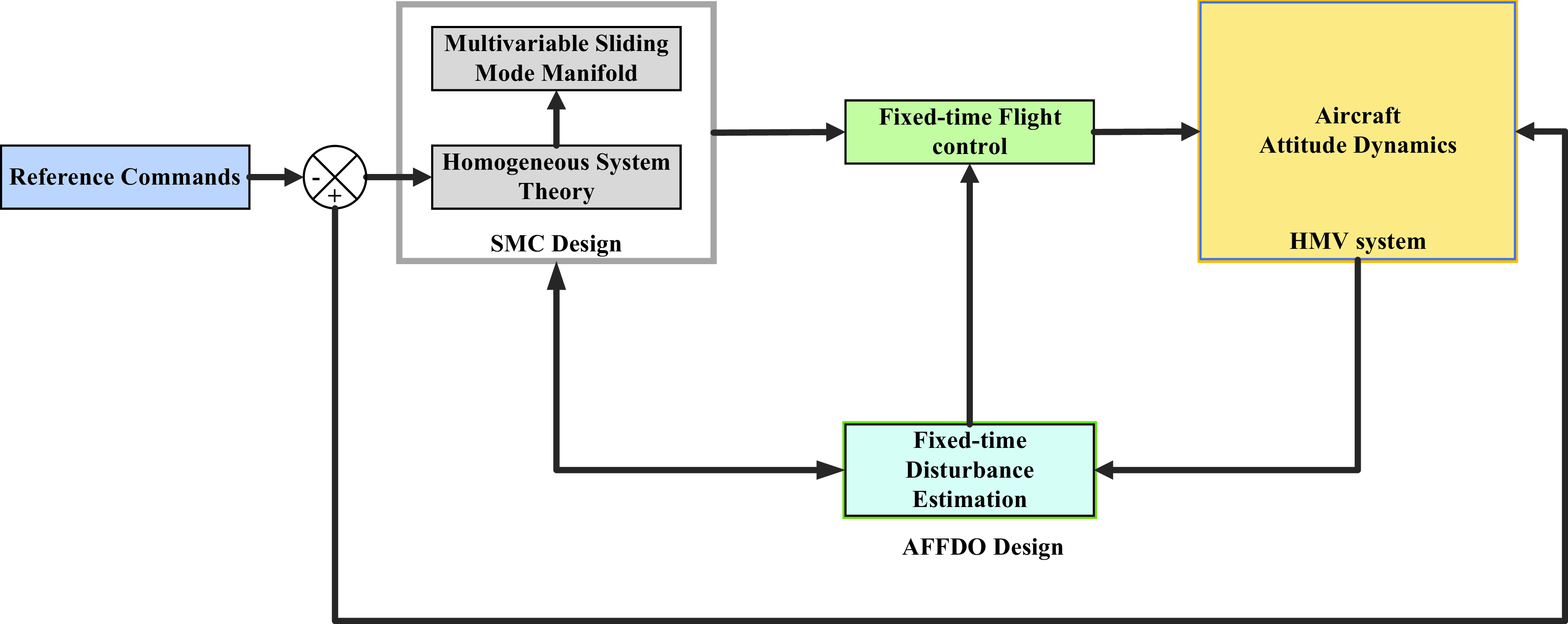
Figure 1. Controller diagram.
3.1 Preparations for controller design
3.1.1 Assumptions for controller design
The following assumptions are proposed.
Assumption 1 ([Reference Zhang, Wang, Tang and Bao31]). The disturbances are bounded, and the maximum value satisfies
Assumption 2 ([Reference Zhang, Wang, Tang and Bao32]). The nonlinear functions
![]() ${f_{ij}},i = 1,2$
${f_{ij}},i = 1,2$
![]() $,j = 1,2,3$
are smooth.
$,j = 1,2,3$
are smooth.
3.1.2 Definitions
Definition 1. Considering the following nonlinear system
The system is said to be fixed-time stable, if for any
![]() ${\boldsymbol{x}}\!\left( 0 \right) \in \Phi $
, the solution of the system converges to the origin within a finite time
${\boldsymbol{x}}\!\left( 0 \right) \in \Phi $
, the solution of the system converges to the origin within a finite time
![]() $T$
, and the settling time is bounded
$T$
, and the settling time is bounded
![]() $T \le {T_{\max }}$
and independent of initial conditions.
$T \le {T_{\max }}$
and independent of initial conditions.
Definition 2 ((Reference Andrieu, Praly and Astolfi33)). A function or a vector field is said to be homogenous in the bi-limit if it is homogenous in 0-limit and
![]() $\infty - {\mathop{\rm limit}\nolimits} $
simultaneously.
$\infty - {\mathop{\rm limit}\nolimits} $
simultaneously.
3.1.3 Lemmas
Lemma 1 ([Reference Zhang, Wang, Tang and Bao31]). For the system (16) and a positive function
![]() $V\!\left( {\boldsymbol{x}} \right)$
, if there exist some positive parameters
$V\!\left( {\boldsymbol{x}} \right)$
, if there exist some positive parameters
![]() $1 \lt m \lt 2$
,
$1 \lt m \lt 2$
,
![]() $n = 2 - m$
,
$n = 2 - m$
,
![]() $l = \frac{\theta }{{\left( {m - 1} \right){T_c}}}$
, such that
$l = \frac{\theta }{{\left( {m - 1} \right){T_c}}}$
, such that
then, the trajectory of the system is fixed time stable with a settling time
![]() $T \le 2{k^{ - 1}}{T_c}$
.
$T \le 2{k^{ - 1}}{T_c}$
.
Proof. The following transformation is employed.
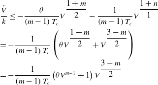 \begin{align}\begin{array}{l}\dfrac{{\dot V}}{k} \le - \dfrac{\theta }{{\left( {m - 1} \right){T_c}}}{V^{\dfrac{{1 + m}}{2}}} - \dfrac{1}{{\left( {m - 1} \right){T_c}}}{V^{\dfrac{{1 + n}}{1}}}\\[10pt] = - \dfrac{1}{{\left( {m - 1} \right){T_c}}}\left( {\theta {V^{\dfrac{{1 + m}}{2}}} + {V^{\dfrac{{3 - m}}{2}}}} \right)\\[10pt] = - \dfrac{1}{{\left( {m - 1} \right){T_c}}}\left( {\theta {V^{m - 1}} + 1} \right){V^{\dfrac{{3 - m}}{2}}}\end{array}\end{align}
Defining
![]() $\bar V = {\theta ^{\frac{1}{2}}}{V^{\frac{{m - 1}}{2}}}$
leads to
$\bar V = {\theta ^{\frac{1}{2}}}{V^{\frac{{m - 1}}{2}}}$
leads to
 \begin{align}\frac{{2{T_c}}}{{k{\theta ^{\frac{1}{2}}}}}\int\limits_{\bar V\!\left( {t = {t_0}} \right)}^{\bar V\!\left( t \right)} {\frac{{d\bar V}}{{{{\bar V}^2} + 1}}} \le {t_0} - t\end{align}
By introducing the function
![]() $\tan \!\left( x \right)$
, one has
$\tan \!\left( x \right)$
, one has
By using
![]() $\bar V\!\left( t \right) = 0$
, the settling time is given by
$\bar V\!\left( t \right) = 0$
, the settling time is given by
Choosing parameter
![]() ${\theta ^{\frac{1}{2}}} \geq \frac{\pi }{2}$
discloses
${\theta ^{\frac{1}{2}}} \geq \frac{\pi }{2}$
discloses
Therefore, the fixed-time convergence is revealed.
Lemma 2 ([Reference Andrieu, Praly and Astolfi33]). For system (16), suppose that the vector
![]() $f\!\left( {\boldsymbol{x}} \right)$
is homogeneous in the bi-limit with associate triples
$f\!\left( {\boldsymbol{x}} \right)$
is homogeneous in the bi-limit with associate triples
![]() $\left( {{r_p},{d_{gp}},{f_p}} \right)$
,
$\left( {{r_p},{d_{gp}},{f_p}} \right)$
,
![]() $p = 0$
or
$p = 0$
or
![]() $p = \infty $
. If the origins of the system
$p = \infty $
. If the origins of the system
![]() ${\dot{\boldsymbol{x}}}\!\left( t \right) = f\!\left( {{\boldsymbol{x}}\!\left( t \right)} \right)$
,
${\dot{\boldsymbol{x}}}\!\left( t \right) = f\!\left( {{\boldsymbol{x}}\!\left( t \right)} \right)$
,
![]() ${{\dot{\boldsymbol{x}}}_0}\!\left( t \right) = {f_0}\!\left( {{\boldsymbol{x}}\!\left( t \right)} \right)$
and
${{\dot{\boldsymbol{x}}}_0}\!\left( t \right) = {f_0}\!\left( {{\boldsymbol{x}}\!\left( t \right)} \right)$
and
![]() ${{\dot{\boldsymbol{x}}}_\infty }\!\left( t \right) = {f_\infty }\!\left( {{\boldsymbol{x}}\!\left( t \right)} \right)$
are global asymptotically stable, then the origin of the system is fixed-time stable in the condition of
${{\dot{\boldsymbol{x}}}_\infty }\!\left( t \right) = {f_\infty }\!\left( {{\boldsymbol{x}}\!\left( t \right)} \right)$
are global asymptotically stable, then the origin of the system is fixed-time stable in the condition of
![]() ${d_{g\infty }} \gt 0 \gt {d_{g0}}$
.
${d_{g\infty }} \gt 0 \gt {d_{g0}}$
.
3.2 AFFDO design
Fuzzy logic system is introduced in the disturbance observer design. The fuzzy rules take the following form [Reference Zhang, Wang, Tang and Bao31]:
![]() $RULE j\,:\,IF\ {x_1}$
is
$RULE j\,:\,IF\ {x_1}$
is
![]() $A_1^j$
and
$A_1^j$
and
![]() $ \ldots $
and
$ \ldots $
and
![]() ${x_n}$
is
${x_n}$
is
![]() $A_n^j$
$A_n^j$
![]() $THEN$
$THEN$
![]() $y$
is
$y$
is
![]() ${B^j}$
${B^j}$
where
![]() $A_1^j, \ldots ,A_n^j$
are the fuzzy sets and
$A_1^j, \ldots ,A_n^j$
are the fuzzy sets and
![]() ${B^j}$
is the output of the
${B^j}$
is the output of the
![]() $j{\mathop{\rm th}\nolimits} $
fuzzy rules. This research employs the centre-of-gravity defuzzification method to build the output of the fuzzy system.
$j{\mathop{\rm th}\nolimits} $
fuzzy rules. This research employs the centre-of-gravity defuzzification method to build the output of the fuzzy system.
 \begin{align}y = \frac{{\sum\limits_{j = 1}^m {{{\rm E}_j}\!\left( {\Pi _{i = 1}^n\Omega _{A_i^j}\!\left( {{x_i}} \right)} \right)} }}{{\sum\limits_{j = 1}^m {\left( {\Pi _{i = 1}^n\Omega _{A_i^j}\!\left( {{x_i}} \right)} \right)} }}\end{align}
where
![]() $\Omega _{A_i^j}\!\left( {{x_i}} \right)$
is the fuzzy membership function of variables
$\Omega _{A_i^j}\!\left( {{x_i}} \right)$
is the fuzzy membership function of variables
![]() ${x_i}$
and
${x_i}$
and
![]() ${\kappa _j}$
is a singleton fuzzy output value.
${\kappa _j}$
is a singleton fuzzy output value.
![]() $m$
is the number of fuzzy rules. Based on the discussion shown above, the output of the fuzzy system is given by
$m$
is the number of fuzzy rules. Based on the discussion shown above, the output of the fuzzy system is given by
where
![]() ${\boldsymbol{\kappa }} = {\left[ {\begin{array}{*{20}{c}}{{\kappa _1}} \cdots {{\kappa _j}} \cdots {{\kappa _m}}\end{array}} \right]^{\rm T}}$
is the adjustable parameter vector.
${\boldsymbol{\kappa }} = {\left[ {\begin{array}{*{20}{c}}{{\kappa _1}} \cdots {{\kappa _j}} \cdots {{\kappa _m}}\end{array}} \right]^{\rm T}}$
is the adjustable parameter vector.
![]() ${\boldsymbol{\psi }} = {\left[ {\begin{array}{*{20}{c}}{{\psi _1}} \cdots {{\psi _j}} \cdots {{\psi _m}}\end{array}} \right]^{\rm T}}$
is the fuzzy basic function vector that is revealed as
${\boldsymbol{\psi }} = {\left[ {\begin{array}{*{20}{c}}{{\psi _1}} \cdots {{\psi _j}} \cdots {{\psi _m}}\end{array}} \right]^{\rm T}}$
is the fuzzy basic function vector that is revealed as
 \begin{align}{\psi _j} = \frac{{\Pi _{i = 1}^n\Omega _{A_i^j}\!\left( {{x_i}} \right)}}{{\sum\limits_{j = 1}^m {\left( {\Pi _{i = 1}^n\Omega _{A_i^j}\!\left( {{x_i}} \right)} \right)} }}\end{align}
Recalling the results of fuzzy control theory, any real continuous function
![]() $f\!\left( x \right)$
defined in a compact set
$f\!\left( x \right)$
defined in a compact set
![]() ${S_c}$
can be approximated by
${S_c}$
can be approximated by
![]() $\mathop {\sup }\limits_{x \in {S_c}} \left| {{{\boldsymbol{\eta}}^{\rm T}}{\boldsymbol{\psi }}\!\left( x \right) - f\!\left( x \right)} \right| \lt \varepsilon $
after applying the fuzzy logic system, where
$\mathop {\sup }\limits_{x \in {S_c}} \left| {{{\boldsymbol{\eta}}^{\rm T}}{\boldsymbol{\psi }}\!\left( x \right) - f\!\left( x \right)} \right| \lt \varepsilon $
after applying the fuzzy logic system, where
![]() $\varepsilon \gt 0$
is a small constant.
$\varepsilon \gt 0$
is a small constant.
Based on the above analysis, we employ a fixed-time technique-based adaptive fuzzy fixed-time disturbance observer to estimate the multisource uncertainties and the terms that are difficult to obtain.
The scalar form is adopted to simplify the observer design procedure for
![]() ${{\boldsymbol{z}}_1} = {\left[ {\begin{array}{*{20}{c}}{{z_{11}}}\quad {{z_{12}}}\quad {{z_{13}}}\end{array}} \right]^{\rm T}}$
. The state and disturbance observers are designed as
${{\boldsymbol{z}}_1} = {\left[ {\begin{array}{*{20}{c}}{{z_{11}}}\quad {{z_{12}}}\quad {{z_{13}}}\end{array}} \right]^{\rm T}}$
. The state and disturbance observers are designed as
where
![]() ${h_{1i}} = {z_{2i}} + {\hat \Delta _{1i}}$
and
${h_{1i}} = {z_{2i}} + {\hat \Delta _{1i}}$
and
![]() ${\hat \Delta _{1i}}$
is the i-th element of the disturbance estimation
${\hat \Delta _{1i}}$
is the i-th element of the disturbance estimation
![]() ${{\boldsymbol{\Delta }}_1}$
in model (14).
${{\boldsymbol{\Delta }}_1}$
in model (14).
According to the universal approximation feature of the fuzzy logic system, we get
where
![]() ${\boldsymbol{\kappa }}_{1i}^*$
represents the optimal value of
${\boldsymbol{\kappa }}_{1i}^*$
represents the optimal value of
![]() ${\kappa _{1i}}$
.
${\kappa _{1i}}$
.
![]() ${\varepsilon _{1i}}$
is the estimation errors of the fuzzy logic system. By using
${\varepsilon _{1i}}$
is the estimation errors of the fuzzy logic system. By using
![]() ${{\boldsymbol{\psi }}_{1i}}\!\left( x \right)$
to indicate the fuzzy basic functions, the optimal and nominal estimation of the disturbance can be expressed as
${{\boldsymbol{\psi }}_{1i}}\!\left( x \right)$
to indicate the fuzzy basic functions, the optimal and nominal estimation of the disturbance can be expressed as
where
![]() $x$
in the function
$x$
in the function
![]() ${{\boldsymbol{\psi }}_{1i}}\!\left( x \right)$
stands for the states in model (10).
${{\boldsymbol{\psi }}_{1i}}\!\left( x \right)$
stands for the states in model (10).
Thus, the estimation error is defined as
Thus, the adaptive law is given by
where
![]() ${\mu _1} \gt 1$
.
${\mu _1} \gt 1$
.
The state and disturbance observer for
![]() ${{\boldsymbol{z}}_2} = {\left[ {\begin{array}{*{20}{c}}{{z_{21}}} {{z_{22}}} {{z_{23}}}\end{array}} \right]^{\rm T}}$
is developed as follows.
${{\boldsymbol{z}}_2} = {\left[ {\begin{array}{*{20}{c}}{{z_{21}}} {{z_{22}}} {{z_{23}}}\end{array}} \right]^{\rm T}}$
is developed as follows.
where
![]() ${h_{2i}} = {F_i} + {\left( {{\boldsymbol{Gu}}} \right)_i} + {\hat \Delta _{2i}}$
.
${h_{2i}} = {F_i} + {\left( {{\boldsymbol{Gu}}} \right)_i} + {\hat \Delta _{2i}}$
.
![]() ${\hat \Delta _{2i}}$
is the i-th element of the disturbance estimation
${\hat \Delta _{2i}}$
is the i-th element of the disturbance estimation
![]() ${{\boldsymbol{\Delta }}_2}$
in model (14).
${{\boldsymbol{\Delta }}_2}$
in model (14).
Employing the fuzzy logic system leads to
where
![]() ${\boldsymbol{\kappa }}_{2i}^*$
is the optimal value of
${\boldsymbol{\kappa }}_{2i}^*$
is the optimal value of
![]() ${{\boldsymbol{\kappa }}_{2i}}$
.
${{\boldsymbol{\kappa }}_{2i}}$
.
![]() ${\varepsilon _{2i}}$
is the estimation error of the fuzzy logic system. The optimal and nominal estimation of the disturbance can be expressed as
${\varepsilon _{2i}}$
is the estimation error of the fuzzy logic system. The optimal and nominal estimation of the disturbance can be expressed as
where
![]() ${{\boldsymbol{\psi }}_{2i}}\!\left( x \right)$
is the fuzzy basic functions.
${{\boldsymbol{\psi }}_{2i}}\!\left( x \right)$
is the fuzzy basic functions.
Thus, the estimation error is indicated by
One can design the adaptive law as follows.
where
![]() ${\mu _2} \gt 1$
.
${\mu _2} \gt 1$
.
Now, the fixed-time observers are successfully developed, where
![]() ${p_i} \gt 1,1 \gt {q_i} \gt 0$
.
${p_i} \gt 1,1 \gt {q_i} \gt 0$
.
![]() ${\lambda _{ij}},i = 1,2.j = 1,2,3,4,5,6$
are positive.
${\lambda _{ij}},i = 1,2.j = 1,2,3,4,5,6$
are positive.
3.3 Fuzzy sliding mode controller design
The fixed-time control theory is adopted since the expression of control input can be directly obtained, and the convergence performance can be verified by the Lyapunov theory.
The multivariable fuzzy sliding mode manifold is designed as
where the parameters are chosen as
 \begin{align}\left\{ \begin{array}{l}{p_1} = p\\[5pt]{p_2} = {\rho _0}\end{array} \right.\end{align}
with the designed coefficients satisfying
![]() ${\rho _0} \in \left( {0,1} \right)$
,
${\rho _0} \in \left( {0,1} \right)$
,
![]() $p \in \left( {0,1} \right)$
,
$p \in \left( {0,1} \right)$
,
![]() $q \gt 1$
.
$q \gt 1$
.
Thus,
![]() ${p_i} \in \left( {0,1} \right)$
and
${p_i} \in \left( {0,1} \right)$
and
![]() ${q_i} \gt 1$
,
${q_i} \gt 1$
,
![]() $i = 1,2$
is obtained. In this paper,
$i = 1,2$
is obtained. In this paper,
![]() ${\boldsymbol{si}}{{\boldsymbol{g}}^p}\!\left( {{{\boldsymbol{z}}_i}} \right) = {\left[ {si{g^p}\!\left( {{z_{i1}}} \right),si{g^p}\!\left( {{z_{i2}}} \right),si{g^p}\!\left( {{z_{i2}}} \right)} \right]^{\rm T}}$
and
${\boldsymbol{si}}{{\boldsymbol{g}}^p}\!\left( {{{\boldsymbol{z}}_i}} \right) = {\left[ {si{g^p}\!\left( {{z_{i1}}} \right),si{g^p}\!\left( {{z_{i2}}} \right),si{g^p}\!\left( {{z_{i2}}} \right)} \right]^{\rm T}}$
and
![]() $si{g^r}\!\left( x \right) = sign\!\left( x \right){\left| x \right|^r}$
are defined.
$si{g^r}\!\left( x \right) = sign\!\left( x \right){\left| x \right|^r}$
are defined.
The derivative of the sliding mode variable
![]() ${\boldsymbol{S}}$
is expressed as
${\boldsymbol{S}}$
is expressed as
Substituting the control-oriented model yields
The controller is given as
where
![]() ${\hat{\boldsymbol{\Delta}}_2}$
is the output from the observers.
${\hat{\boldsymbol{\Delta}}_2}$
is the output from the observers.
The robust controller is developed in this step.
4.0 Stability analysis
4.1 Convergence of the disturbance estimation
Theorem 1. For the control-oriented model and the designed AFFDO, the estimation error will converge to the origin within fixed-time
![]() ${T_i} \le 2{T_{ic}}$
, if the key parameters satisfy
${T_i} \le 2{T_{ic}}$
, if the key parameters satisfy
![]() ${\mu _i} \gt 1$
,
${\mu _i} \gt 1$
,
![]() $0 \lt {p_{0,i}} \lt \frac{2}{{{\mu _i} + 1}}$
,
$0 \lt {p_{0,i}} \lt \frac{2}{{{\mu _i} + 1}}$
,
![]() $\lambda _{i,1} = \frac{{{\theta _i}}}{{\left( {{\mu _i} + 1} \right){p_{0,i}}{T_{ic}}}}$
and
$\lambda _{i,1} = \frac{{{\theta _i}}}{{\left( {{\mu _i} + 1} \right){p_{0,i}}{T_{ic}}}}$
and
![]() $\lambda _{i,2} = \frac{1}{{\left( {{\mu _i} + 1} \right){p_{0,i}}{T_{ic}}}}$
. The settling time is directly designed in the parameters.
$\lambda _{i,2} = \frac{1}{{\left( {{\mu _i} + 1} \right){p_{0,i}}{T_{ic}}}}$
. The settling time is directly designed in the parameters.
Proof. The Lyapunov function for
![]() ${\tilde z_{2i}}$
and
${\tilde z_{2i}}$
and
![]() $\tilde \kappa _{2i}$
is selected as
$\tilde \kappa _{2i}$
is selected as
where
![]() $\tilde{\boldsymbol{\kappa}}_{2i} = {\boldsymbol{\kappa }}_{2i}^{\rm{*}} - \hat{\boldsymbol{\kappa}}_{2i}$
,
$\tilde{\boldsymbol{\kappa}}_{2i} = {\boldsymbol{\kappa }}_{2i}^{\rm{*}} - \hat{\boldsymbol{\kappa}}_{2i}$
,
![]() ${\mu _2} \gt 1$
.
${\mu _2} \gt 1$
.
The proof is divided into two stages.
Stage 1. The derivative of the function is represented by
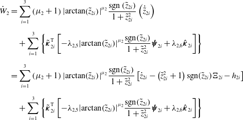 \begin{align}{{\dot W}_2} & = \sum\limits_{i = 1}^3 {\left( {{\mu _2} + 1} \right){{\left| {\arctan \!\left( {{{\tilde z}_{2i}}} \right)} \right|}^{{\mu _2}}}\frac{{{\mathop{\rm sgn}} \left( {\tilde z_{2i}} \right)}}{{1 + \tilde z_{2i}^2}}\left( {\dot{\tilde{z}}_{2i}} \right)} \nonumber\\[5pt] & \quad + \sum\limits_{i = 1}^3 {\left\{ {\tilde{\boldsymbol{\kappa}}_{2i}^{\rm T}\left[ { - {\lambda _{2,5}}{{\left| {\arctan \!\left( {{{\tilde z}_{2i}}} \right)} \right|}^{{\mu _2}}}\frac{{{\mathop{\rm sgn}} \!\left( {\tilde z_{2i}} \right)}}{{1 + \tilde z_{2i}^2}}{{\boldsymbol{\psi }}_{2i}} + {\lambda _{2,6}}{{\hat{\boldsymbol{\kappa}}}_{2i}}} \right]} \right\}} \nonumber\\[5pt] & = \sum\limits_{i = 1}^3 \left( {{\mu _2} + 1} \right){{\left| {\arctan \!\left( {{{\tilde z}_{2i}}} \right)} \right|}^{{\mu _2}}}\frac{{{\mathop{\rm sgn}} \!\left( {\tilde z_{2i}} \right)}}{{1 + \tilde z_{2i}^2}}\left[ {{{\dot z}_{2i}} } - {\left( {\tilde z_{2i}^2 + 1} \right){\mathop{\rm sgn}} ({{\tilde z}_{2i}}){\Xi _{2i}} - {h_{2i}}} \right] \\[5pt] & \quad +\sum\limits_{i = 1}^3 {\left\{ {\tilde{\boldsymbol{\kappa}}_{2i}^{\rm T}\left[ { - {\lambda _{2,5}}{{\left| {\arctan \!\left( {{{\tilde z}_{2i}}} \right)} \right|}^{{\mu _2}}}\frac{{{\mathop{\rm sgn}} \!\left( {\tilde z_{2i}} \right)}}{{1 + \tilde z_{2i}^2}}{{\boldsymbol{\psi }}_{2i}} + {\lambda _{2,6}}{{\hat{\boldsymbol{\kappa}}}_{2i}}} \right]} \right\}} \nonumber\end{align}
With the help of the fuzzy logic system, one gets
 \begin{align}{{\dot W}_2} & = \sum\limits_{i = 1}^3 \left( {{\mu _2} + 1} \right){{\left| {\arctan \!\left( {{{\tilde z}_{2i}}} \right)} \right|}^{{\mu _2}}}\frac{{{\mathop{\rm sgn}} \!\left( {\tilde z_{2i}} \right)}}{{1 + \tilde z_{2i}^2}}\left[ {{\boldsymbol{\kappa }}_{2i}^{*{\rm T}}{{\boldsymbol{\psi }}_{2i}}\!\left( x \right)} + {\varepsilon _{{\rm{2}}i}} - {\left( {\tilde z_{2i}^2 + 1} \right){\mathop{\rm sgn}} ({{\tilde z}_{2i}}){\Xi _{2i}} - \hat{\boldsymbol{\kappa}}_{2i}^{\rm T}{{\boldsymbol{\psi }}_{2i}}\!\left( x \right)} \right] \nonumber\\[5pt]& + \sum\limits_{i = 1}^3 {\left\{ {\tilde{\boldsymbol{\kappa}}_{2i}^{\rm T}\left[ { - {\lambda _{2,5}}{{\left| {\arctan \!\left( {{{\tilde z}_{2i}}} \right)} \right|}^{{\mu _2}}}\frac{{{\mathop{\rm sgn}} \!\left( {\tilde z_{2i}} \right)}}{{1 + \tilde z_{2i}^2}}{{\boldsymbol{\psi }}_{2i}} + {\lambda _{2,6}}{{\hat{\boldsymbol{\kappa}}}_{2i}}} \right]} \right\}}\end{align}
 \begin{align}{{\dot W}_2} & = \sum\limits_{i = 1}^3 \left( {{\mu _2} + 1} \right){{\left| {\arctan \!\left( {{{\tilde z}_{2i}}} \right)} \right|}^{{\mu _2}}}\frac{{{\mathop{\rm sgn}} \!\left( {\tilde z_{2i}} \right)}}{{1 + \tilde z_{2i}^2}}\left[ {\tilde{\boldsymbol{\kappa}}_{2i}^{\rm T}{{\boldsymbol{\psi }}_{2i}}\!\left( x \right) } + {\varepsilon _{{\rm{2}}i}} - {\left( {\tilde z_{2i}^2 + 1} \right){\mathop{\rm sgn}} ({{\tilde z}_{2i}}){\Xi _{2i}}} \right] \nonumber\\[5pt]& \quad + \sum\limits_{i = 1}^3 {\left\{ {\tilde{\boldsymbol{\kappa}}_{2i}^{\rm T}\left[ { - {\lambda _{2,5}}{{\left| {\arctan \!\left( {{{\tilde z}_{2i}}} \right)} \right|}^{{\mu _2}}}\frac{{{\mathop{\rm sgn}} \!\left( {\tilde z_{2i}} \right)}}{{1 + \tilde z_{2i}^2}}{{\boldsymbol{\psi }}_{2i}} + {\lambda _{2,6}}{{\hat{\boldsymbol{\kappa}}}_{2i}}} \right]} \right\}} \end{align}
Choosing parameter
![]() ${\lambda _{2,5}} = {\mu _2} + 1$
results in
${\lambda _{2,5}} = {\mu _2} + 1$
results in
 \begin{align}{{\dot W}_2} & = \sum\limits_{i = 1}^3 \left( {{\mu _2} + 1} \right){{\left| {\arctan \!\left( {{{\tilde z}_{2i}}} \right)} \right|}^{{\mu _2}}}\frac{{{\mathop{\rm sgn}} \!\left( {\tilde z_{2i}} \right)}}{{1 + \tilde z_{2i}^2}}\left[ {\varepsilon _{{\rm{2}}i}} - \left( {\tilde z_{2i}^2 + 1} \right){\mathop{\rm sgn}} ({{\tilde z}_{2i}}){\Xi _{2i}} \right] + \sum\limits_{i = 1}^3 {\left[ {\tilde{\boldsymbol{\kappa}}_{2i}^{\rm T}{\lambda _{2,6}}{{\hat{\boldsymbol{\kappa}}}_{2i}}} \right]} \nonumber\\[5pt]& \le \sum\limits_{i = 1}^3 \left( {{\mu _2} + 1} \right){{\left| {\arctan \!\left( {{{\tilde z}_{2i}}} \right)} \right|}^{{\mu _2}}}\frac{{{\mathop{\rm sgn}} \!\left( {\tilde z_{2i}} \right)}}{{1 + \tilde z_{2i}^2}}{\varepsilon _{{\rm{2}}i}} - \sum\limits_{i = 1}^3 \left( {{\mu _2} + 1} \right){{\left| {\arctan \!\left( {{{\tilde z}_{2i}}} \right)} \right|}^{{\mu _2}}}{\Xi _{2i}} + \sum\limits_{i = 1}^3 {\left[ {\tilde{\boldsymbol{\kappa}}_{2i}^{\rm T}{\lambda _{2,6}}{{\hat{\boldsymbol{\kappa}}}_{2i}}} \right]} \nonumber\\[5pt]& \le \sum\limits_{i = 1}^3 {\left( {{\mu _2} + 1} \right){{\left| {\arctan \!\left( {{{\tilde z}_{2i}}} \right)} \right|}^{{\mu _2}}}{\mathop{\rm sgn}} \!\left( {\tilde z_{2i}} \right){\varepsilon _{{\rm{2}}i}}} - \sum\limits_{i = 1}^3 {\left( {{\mu _2} + 1} \right){{\left| {\arctan \!\left( {{{\tilde z}_{2i}}} \right)} \right|}^{{\mu _2}}}{\Xi _{2i}}}\\& \quad + \frac{1}{2}\sum\limits_{i = 1}^3 {\left( { - {\lambda _{2,6}}\tilde{\boldsymbol{\kappa}}_{2i}^{\rm T}{{\tilde{\boldsymbol{\kappa}}}_{2i}} + {\lambda _{2,6}}{\boldsymbol{\kappa }}_{2i}^*{\boldsymbol{\kappa }}_{2i}^*} \right)} \nonumber\end{align}
Introducing the expression of
![]() ${\Xi _{2i}}$
discloses
${\Xi _{2i}}$
discloses
 \begin{align}{{\dot W}_2} & \le \sum\limits_{i = 1}^3 {\left( {{\mu _2} + 1} \right){{\left| {\arctan \!\left( {{{\tilde z}_{2i}}} \right)} \right|}^{{\mu _2}}}{\mathop{\rm sgn}} \!\left( {\tilde z_{2i}} \right){\varepsilon _{{\rm{2}}i}}} - \sum\limits_{i = 1}^3 {\left( {{\mu _2} + 1} \right)\lambda _{2,1}{{\left| {\arctan \!\left( {{{\tilde z}_{2i}}} \right)} \right|}^{{\mu _2} + {p_2}}}}\nonumber\\[5pt]& \quad - \sum\limits_{i = 1}^3 {\left( {{\mu _2} + 1} \right)\lambda _{2,2}{{\left| {\arctan \!\left( {{{\tilde z}_{2i}}} \right)} \right|}^{{\mu _2} + {q_2}}}} - \sum\limits_{i = 1}^3 {\left( {{\mu _2} + 1} \right)\lambda _{2,3}{{\left| {\arctan \!\left( {{{\tilde z}_{2i}}} \right)} \right|}^{{\mu _2}}}\left| {{\mathop{\rm sgn}} \!\left( {{{\tilde z}_{2i}}} \right)} \right|} \\[5pt]& \quad +\frac{1}{2}\sum\limits_{i = 1}^3 {\left( { - {\lambda _{2,6}}\tilde{\boldsymbol{\kappa}}_{2i}^{\rm T}{{\tilde{\boldsymbol{\kappa}}}_{2i}} + {\lambda _{2,6}}{\boldsymbol{\kappa }}_{2i}^*{\boldsymbol{\kappa }}_{2i}^*} \right)} \nonumber\end{align}
The following parameter is employed
It can be further obtained that
 \begin{align}{{\dot W}_2} & \le - \sum\limits_{i = 1}^3 {\left( {{\mu _2} + 1} \right)\lambda _{2,1}{{\left| {\arctan \!\left( {{{\tilde z}_{2i}}} \right)} \right|}^{{\mu _2} + {p_2}}}} - \sum\limits_{i = 1}^3 {\left( {{\mu _2} + 1} \right)\lambda _{2,2}{{\left| {\arctan \!\left( {{{\tilde z}_{2i}}} \right)} \right|}^{{\mu _2} + {q_2}}}} \nonumber\\[5pt]& \quad + \frac{1}{2}\sum\limits_{i = 1}^3 {\left( { - {\lambda _{2,6}}\tilde{\boldsymbol{\kappa}}_{2i}^{\rm T}{{\tilde \kappa }_{2i}} + {\lambda _{2,6}}{\boldsymbol{\kappa }}_{2i}^{*{\rm T}}\kappa _{2i}^*} \right)} \end{align}
The parameters are transformed to
The derivative of the Lyapunov function is rewritten as
 \begin{align}{{\dot W}_2} & \le - \sum\limits_{i = 1}^3 \left( {{\mu _2} + 1} \right)\lambda _{2,1}{{\left[ {{{\left| {\arctan \!\left( {{{\tilde z}_{2i}}} \right)} \right|}^{{\mu _2} + 1}}} \right]}^{1 + \frac{{{p_{0,2}}}}{2}}} - {\sum\limits_{i = 1}^3 {\left( {{\mu _2} + 1} \right)\lambda _{2,2}\left[ {{{\left| {\arctan \!\left( {{{\tilde z}_{2i}}} \right)} \right|}^{{\mu _2} + 1}}} \right]} ^{1 - \frac{{{p_{0,2}}}}{2}}} \nonumber\\[5pt]& + \frac{1}{2}\sum\limits_{i = 1}^3 {\left( { - {\lambda _{2,6}}\tilde{\boldsymbol{\kappa}}_{2i}^{\rm T}{{\tilde{\boldsymbol{\kappa}}}_{2i}} + {\lambda _{2,6}}{\boldsymbol{\kappa }}_{2i}^{*{\rm T}}{\boldsymbol{\kappa }}_{2i}^*} \right)} \end{align}
Considering the following expression
where
![]() $1 \gt a \gt 0,b \gt 1$
.
$1 \gt a \gt 0,b \gt 1$
.
Therefore
where
![]() $\underline \lambda _{2,1} = \min \!\left\{ {\lambda _{2,1},\lambda _{2,2}} \right\}$
. Introducing
$\underline \lambda _{2,1} = \min \!\left\{ {\lambda _{2,1},\lambda _{2,2}} \right\}$
. Introducing
![]() ${m_{0,2}}$
to indicate
${m_{0,2}}$
to indicate
![]() $\frac{1}{2}\sum\limits_{i = 1}^3 {{\lambda _{2,6}}\kappa _{2i}^{*{\rm T}}\kappa _{2i}^*} $
shows
$\frac{1}{2}\sum\limits_{i = 1}^3 {{\lambda _{2,6}}\kappa _{2i}^{*{\rm T}}\kappa _{2i}^*} $
shows
Using
![]() $\underline \lambda _{2,2} = \min \!\left\{ {\left( {{\mu _2} + 1} \right)\underline \lambda _{2,1},{\lambda _{2,4}}{\lambda _{2,6}}} \right\}$
leads to
$\underline \lambda _{2,2} = \min \!\left\{ {\left( {{\mu _2} + 1} \right)\underline \lambda _{2,1},{\lambda _{2,4}}{\lambda _{2,6}}} \right\}$
leads to
Thus,
![]() ${W_2}$
,
${W_2}$
,
![]() ${\tilde z_{2i}}$
and
${\tilde z_{2i}}$
and
![]() ${\tilde \kappa _{2i}}$
are bounded. The full estimation errors
${\tilde \kappa _{2i}}$
are bounded. The full estimation errors
![]() ${\bar \varepsilon _{2i}} = \tilde \kappa _{2i}^{\rm T}{{\boldsymbol{\psi }}_{2i}}\!\left( x \right) + {\varepsilon _{2i}}$
are also bounded.
${\bar \varepsilon _{2i}} = \tilde \kappa _{2i}^{\rm T}{{\boldsymbol{\psi }}_{2i}}\!\left( x \right) + {\varepsilon _{2i}}$
are also bounded.
Stage 2. The Lyapunov function for
![]() ${\tilde z_{2i}}$
is designed as follows.
${\tilde z_{2i}}$
is designed as follows.
The derivative of
![]() ${V_2}$
is given by
${V_2}$
is given by
 \begin{align}{V_2} & = \left( {{\mu _2} + 1} \right)\sum\limits_{i = 1}^3 {\left[ {{{\left| {\arctan \!\left( {{{\tilde z}_{2i}}} \right)} \right|}^{{\mu _2}}}\frac{{{\mathop{\rm sgn}} \left( {{{\tilde z}_{2i}}} \right)}}{{1 + \tilde z_{2i}^2}}{{\dot{\tilde{z}}}_{2i}}} \right]} \nonumber\\[5pt]& = \left( {{\mu _2} + 1} \right)\sum\limits_{i = 1}^3 {\left[ {{{\left| {\arctan \!\left( {{{\tilde z}_{2i}}} \right)} \right|}^{{\mu _2}}}{\Xi _{2i}}} \right]} + \left( {{\mu _2} + 1} \right)\sum\limits_{i = 1}^3 {{{\left| {\arctan \!\left( {{{\tilde z}_{2i}}} \right)} \right|}^{{\mu _2}}}\frac{{{\mathop{\rm sgn}} \!\left( {{{\tilde z}_{2i}}} \right)}}{{1 + \tilde z_{2i}^2}}\!\left( {{\Delta _{2i}} - {{\hat \Delta }_{2i}}} \right)} \end{align}
By introducing the fuzzy logic system, one gets
 \begin{align}{{\dot V}_2} & = \left( {{\mu _2} + 1} \right)\sum\limits_{i = 1}^3 {\left[ {{{\left| {\arctan \!\left( {{{\tilde z}_{2i}}} \right)} \right|}^{{\mu _2}}}\frac{{{\mathop{\rm sgn}} \!\left( {{{\tilde z}_{2i}}} \right)}}{{1 + \tilde z_{2i}^2}}{{\dot{\tilde{z}}}_{2i}}} \right]} \nonumber\\[5pt]& = \left( {{\mu _2} + 1} \right)\sum\limits_{i = 1}^3 {\left[ {{{\left| {\arctan \!\left( {{{\tilde z}_{2i}}} \right)} \right|}^{{\mu _2}}}{\Xi _{2i}}} \right]} + \left( {{\mu _2} + 1} \right)\sum\limits_{i = 1}^3 {{{\left| {\arctan \!\left( {{{\tilde z}_{2i}}} \right)} \right|}^{{\mu _2}}}\frac{{{\mathop{\rm sgn}} \!\left( {{{\tilde z}_{2i}}} \right)}}{{1 + \tilde z_{2i}^2}}\left( {\tilde \kappa _{2i}^{\rm T}{{\boldsymbol{\psi }}_{2i}}\!\left( x \right) + {\varepsilon _{2i}}} \right)}\end{align}
Substituting the expression
![]() ${\Xi _{2i}}$
into
${\Xi _{2i}}$
into
![]() ${\dot V_2}$
reveals
${\dot V_2}$
reveals
 \begin{align}{{\dot V}_2} & = \left( {{\mu _2} + 1} \right)\sum\limits_{i = 1}^3 {\left[ {{{\left| {\arctan \!\left( {{{\tilde z}_{2i}}} \right)} \right|}^{{\mu _2}}}\frac{{{\mathop{\rm sgn}} \!\left( {{{\tilde z}_{2i}}} \right)}}{{1 + \tilde z_{2i}^2}}{{\dot{\tilde{z}}}_{2i}}} \right]} \nonumber\\[3pt]& \le - \sum\limits_{i = 1}^3 {\left( {{\mu _2} + 1} \right)\lambda _{2,1}{{\left| {\arctan \!\left( {{{\tilde z}_{2i}}} \right)} \right|}^{{\mu _2} + {p_2}}}} - \sum\limits_{i = 1}^3 {\left( {{\mu _2} + 1} \right)\lambda _{2,2}{{\left| {\arctan \!\left( {{{\tilde z}_{2i}}} \right)} \right|}^{{\mu _2} + {q_2}}}}\nonumber\\[3pt]& - \sum\limits_{i = 1}^3 {\left( {{\mu _2} + 1} \right)\lambda _{2,3}{{\left| {\arctan \!\left( {{{\tilde z}_{2i}}} \right)} \right|}^{{\mu _2}}}\left| {{\mathop{\rm sgn}} \!\left( {{{\tilde z}_{2i}}} \right)} \right|} + \left( {{\mu _2} + 1} \right)\sum\limits_{i = 1}^3 {{{\left| {\arctan \!\left( {{{\tilde z}_{2i}}} \right)} \right|}^{{\mu _2}}}{\mathop{\rm sgn}} \!\left( {{{\tilde z}_{2i}}} \right)\left( {\tilde \kappa _{2i}^{\rm T}{{\boldsymbol{\psi }}_{2i}}\!\left( x \right) + {\varepsilon _{2i}}} \right)} \end{align}
Then, the following condition for
![]() $\lambda _{2,3}$
is adopted
$\lambda _{2,3}$
is adopted
It leads to
Choosing the following parameters
The derivative of the Lyapunov function is rewritten
 \begin{align}{{\dot V}_2} & \le - \frac{1}{{{p_{0,2}}{T_{2c}}}}{\sum\limits_{i = 1}^3 {{\theta _2}\left[ {{{\left| {\arctan \!\left( {{{\tilde z}_{2i}}} \right)} \right|}^{{\mu _2} + 1}}} \right]} ^{1 + \frac{{{p_{0,2}}}}{2}}} - \frac{1}{{{p_{0,2}}{T_{2c}}}}{\sum\limits_{i = 1}^3 {\left[ {{{\left| {\arctan \!\left( {{{\tilde z}_{2i}}} \right)} \right|}^{{\mu _2} + 1}}} \right]} ^{1 - \frac{{{p_{0,2}}}}{2}}}\nonumber\\[5pt]& \le - \frac{{{\theta _2}}}{{{p_{0,2}}{T_{2c}}}}{3^{ - \frac{{{p_{0,2}}}}{2}}}{V_2}^{1 + \frac{{{p_{0,2}}}}{2}} - \frac{1}{{{p_{0,2}}{T_{2c}}}}{V_2}^{1 - \frac{{{p_{0,2}}}}{2}}\end{align}
Introducing
![]() $\bar \theta _2^2 = {\theta _2}{3^{ - \frac{{{p_{0,2}}}}{2}}}$
,
$\bar \theta _2^2 = {\theta _2}{3^{ - \frac{{{p_{0,2}}}}{2}}}$
,
![]() $V_{2,{{\bar \theta }_2}}^2 = \bar \theta _2^2{\left( {V_2^{\frac{{{p_{0,2}}}}{2}}} \right)^2}$
and lemma 1, it is obvious that the estimation error will converge to the origin within fixed time. The settling time is estimated by
$V_{2,{{\bar \theta }_2}}^2 = \bar \theta _2^2{\left( {V_2^{\frac{{{p_{0,2}}}}{2}}} \right)^2}$
and lemma 1, it is obvious that the estimation error will converge to the origin within fixed time. The settling time is estimated by
Therefore,
![]() ${{\hat{\boldsymbol{z}}}_2}$
tracks
${{\hat{\boldsymbol{z}}}_2}$
tracks
![]() ${{\boldsymbol{z}}_2}$
for any time
${{\boldsymbol{z}}_2}$
for any time
![]() $t \geq {T_2}$
. Note that the disturbance observers have a similar structure. Using the same method, it is easy to demonstrate the fixed time convergence of
$t \geq {T_2}$
. Note that the disturbance observers have a similar structure. Using the same method, it is easy to demonstrate the fixed time convergence of
![]() ${{\tilde{\boldsymbol{z}}}_1}$
. For sake of saving space, the details are omitted.
${{\tilde{\boldsymbol{z}}}_1}$
. For sake of saving space, the details are omitted.
Since the state estimation error will converge to origin within fixed time
![]() ${T_i}$
for any state
${T_i}$
for any state
![]() ${z_{ij}}$
, the following expression is established according to the control-oriented model and the disturbance observer.
${z_{ij}}$
, the following expression is established according to the control-oriented model and the disturbance observer.
Therefore, we can conclude the disturbance estimation tracks the actual disturbance in the fixed time
![]() ${T_i}$
.
${T_i}$
.
The convergence of the adaptive fuzzy fixed-time disturbance observer is illustrated via Lyapunov theory. It is feasible to achieve disturbance compensation.
Remark 1. In research [Reference Basin, Bharath Panathula and Shtessel34], a fixed time controller is successfully proposed, achieving the significant development. This method has been successfully applied to hypersonic vehicles in [Reference Wang, Guo, Tang and Qi37]. The settling time is estimated by
 \begin{align}{T_f} \le \left( {\frac{1}{{{\lambda _2}\!\left( {p - 1} \right){\varepsilon ^{p - 1}}}} + \frac{{2{{\left( {\sqrt n \varepsilon } \right)}^{\frac{1}{2}}}}}{{{\lambda _1}}}} \right)\left( {1 + \frac{M}{{m\!\left( {1 - \frac{{\sqrt {2\alpha } }}{{{\lambda _1}}}} \right)}}} \right)\end{align}
It is clear that the method in this paper leads to a more explicit settling time compared to the result in [Reference Basin, Bharath Panathula and Shtessel34] since the latter is composed of several parameters. These parameters contribute to converge rate. If a specific convergence time is demanded in the design procedure, it is complicated to finish the work. Thus, one can conclude the convergence time of disturbance observer and the sliding mode variable can be directly specified in the design procedure. The stability of the sliding mode variable will be demonstrated later.
4.2 Convergence of the tracking error
Theorem 2. For the control-oriented model, the sliding mode variable will converge to the origin within fixed-time if the parameters satisfy
![]() $2 \gt m \gt 1$
,
$2 \gt m \gt 1$
,
![]() $n = 2 - m$
,
$n = 2 - m$
,
![]() ${l_2} = \frac{{{c_1}}}{{\left( {m - 1} \right){T_d}}}$
,
${l_2} = \frac{{{c_1}}}{{\left( {m - 1} \right){T_d}}}$
,
![]() ${l_3} = \frac{1}{{\left( {m - 1} \right){T_d}}}$
. The settling time satisfies
${l_3} = \frac{1}{{\left( {m - 1} \right){T_d}}}$
. The settling time satisfies
![]() $T \le {T_d}$
, which is more explicit than the conventional fixed-time control.
$T \le {T_d}$
, which is more explicit than the conventional fixed-time control.
Proof. We firstly illustrate the convergence of the sliding mode variable.
The derivative is of the designed Lyapunov function is
Taking the expression of the sliding mode variable results in
 \begin{align}\frac{{{{\dot V}_3}}}{2} & = {{\boldsymbol{S}}^{\rm T}}\!\left( {{{\dot{\boldsymbol{z}}}_2} + {{{\dot{\hat{\boldsymbol\Delta}}}}_1} + {{\boldsymbol{\sigma }}_1} + {{\boldsymbol{\sigma }}_2}} \right)\nonumber\\[5pt]& = {{\boldsymbol{S}}^{\rm T}}\!\left[ {{\boldsymbol{F}} + {\boldsymbol{Gu}}\!\left( t \right) + {{\boldsymbol{\sigma }}_1} + {{\boldsymbol{\sigma }}_2} + {{\boldsymbol{\Delta }}_2} + {{{\dot{\hat{\boldsymbol\Delta}}}}_1}} \right]\end{align}
Substituting the designed controller shows
 \begin{align}\frac{{{{\dot V}_3}}}{2} & = {{\boldsymbol{S}}^{\rm T}}\!\left[ {{\boldsymbol{F}} + {{\boldsymbol{\sigma }}_1} + {{\boldsymbol{\sigma }}_2} + {{\boldsymbol{\Delta }}_2} + {{{\dot{\hat{\boldsymbol\Delta}}}}_1}} \right] - {{\boldsymbol{S}}^{\rm T}}{\boldsymbol{G}}\!\left[ {{{\boldsymbol{G}}^{ - 1}}\!\left( {{\boldsymbol{F}} + } {{{\boldsymbol{\sigma }}_1} + {{\boldsymbol{\sigma }}_2} + {{\boldsymbol{\upsilon }}_{rob}} + {{\boldsymbol{\upsilon }}_{comp}}} \right)} \right]\nonumber\\[5pt]& = {{\boldsymbol{S}}^{\rm T}}\!\left( {{{\boldsymbol{\Delta }}_2} - {{\hat{\boldsymbol{\Delta}}}_2}} \right) - {{\boldsymbol{S}}^{\rm T}}{{\boldsymbol{\upsilon }}_{rob}}\!\left( t \right)\end{align}
Since the disturbances are eliminated for any time
![]() $t \gt {T_1} + {T_2}$
, one gets
$t \gt {T_1} + {T_2}$
, one gets
The
![]() ${\tilde{\boldsymbol{\Delta}}_2}$
is the full estimation error of the fuzzy logic system. It is obvious that
${\tilde{\boldsymbol{\Delta}}_2}$
is the full estimation error of the fuzzy logic system. It is obvious that
![]() $\left| {{\tilde{\boldsymbol{\Delta}}_2}} \right|$
is proven to be zero when one illustrates the stability of the adaptive fuzzy fixed-time disturbance observer.
$\left| {{\tilde{\boldsymbol{\Delta}}_2}} \right|$
is proven to be zero when one illustrates the stability of the adaptive fuzzy fixed-time disturbance observer.
It brings out
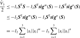 \begin{align}\frac{{{{\dot V}_3}}}{2} & \le - {l_1}{{\boldsymbol{S}}^{\rm T}}{\boldsymbol{S}} - {l_2}{{\boldsymbol{S}}^{\rm T}}{\boldsymbol{si}}{{\boldsymbol{g}}^m}\!\left( {\boldsymbol{S}} \right) - {l_3}{{\boldsymbol{S}}^{\rm T}}{\boldsymbol{si}}{{\boldsymbol{g}}^n}\!\left( {\boldsymbol{S}} \right)\nonumber\\[3pt] & \le - {l_2}{{\boldsymbol{S}}^{\rm T}}{\boldsymbol{si}}{{\boldsymbol{g}}^m}\!\left( {\boldsymbol{S}} \right) - {l_3}{{\boldsymbol{S}}^{\rm T}}{\boldsymbol{si}}{{\boldsymbol{g}}^n}\left( {\boldsymbol{S}} \right)\nonumber\\[3pt] & = - {l_2}\sum\limits_{i = 1}^3 {\left| {{s_i}} \right|} {\left| {s_i} \right|^m} - {l_3}\sum\limits_{i = 1}^3 {\left| {{s_i}} \right|} {\left| {s_i} \right|^n} \end{align}
In order to obtain the fixed-time convergence of the sliding mode variable, the following parameters is introduced.
Therefore,
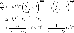 \begin{align}\frac{{{{\dot V}_3}}}{2} & \le - {l_2}{3^{\frac{{1 - m}}{2}}}{\left( {\sum\limits_{i = 1}^3 {{{\left| {s_i} \right|}^2}} } \right)^{\frac{{m + 1}}{2}}} - {l_3}{\left( {\sum\limits_{i = 1}^3 {{{\left| {s_i} \right|}^2}} } \right)^{\frac{{n + 1}}{2}}}\nonumber\\[3pt]& \le - {l_2}{3^{\frac{{1 - m}}{2}}}{V_3}^{\frac{{m + 1}}{2}} - {l_3}{V_3}^{\frac{{n + 1}}{2}}\nonumber\\[3pt]& \le \frac{{{c_1}}}{{\left( {m - 1} \right){T_d}}}{3^{\frac{{1 - m}}{2}}}{V_3}^{\frac{{m + 1}}{2}} - \frac{1}{{\left( {m - 1} \right){T_d}}}{V_3}^{\frac{{3 - m}}{2}}\end{align}
with
![]() $\bar c_1^2 = {c_1}{3^{\frac{{1 - m}}{2}}}$
,
$\bar c_1^2 = {c_1}{3^{\frac{{1 - m}}{2}}}$
,
![]() $V_{3,{{\bar c}_1}}^2 = \bar c_1^2{\left( {V_3^{\frac{{m - 1}}{2}}} \right)^2}$
and lemma 1, the sliding mode will converge to the origin within following settling time.
$V_{3,{{\bar c}_1}}^2 = \bar c_1^2{\left( {V_3^{\frac{{m - 1}}{2}}} \right)^2}$
and lemma 1, the sliding mode will converge to the origin within following settling time.
Theorem 3. After the convergence of the sliding mode variable and the estimation errors, the tracking error will converge to the origin within fixed-time according to the control-oriented mode of the HMV.
Proof. Since
![]() ${\boldsymbol{S}} = 0$
is valid, one gets
${\boldsymbol{S}} = 0$
is valid, one gets
 \begin{align}\left\{ \begin{array}{l}{{\dot{\boldsymbol{z}}}_1} = {{\boldsymbol{z}}_2} + {{\boldsymbol{\Delta }}_1} = {{\boldsymbol{z}}_2} + {{\hat{\boldsymbol{\Delta}}}_1} + {\tilde{\boldsymbol{\Delta}}_1}\\[5pt]{{\boldsymbol{z}}_2} + {{\hat{\boldsymbol{\Delta}}}_1} = - \int_0^t {{{\boldsymbol{\sigma }}_1}} d\tau - \int_0^t {{{\boldsymbol{\sigma }}_2}} d\tau \end{array} \right.\end{align}
The fixed-time convergence of the estimation error has been proven, leading to
![]() ${\tilde{\boldsymbol{\Delta}}_1} = 0$
. We obtain the following expression by defining
${\tilde{\boldsymbol{\Delta}}_1} = 0$
. We obtain the following expression by defining
![]() ${\bar{\boldsymbol{z}}_1} = {{\boldsymbol{z}}_1}$
.
${\bar{\boldsymbol{z}}_1} = {{\boldsymbol{z}}_1}$
.
 \begin{align}\left\{ \begin{array}{l}{\dot{\bar{\boldsymbol{z}}}_1} = {{\bar{\boldsymbol{z}}}_2}\\[5pt]{\dot{\bar{\boldsymbol{z}}}_2} = - {k_1}\!\left[ {{\boldsymbol{si}}{{\boldsymbol{g}}^{{p_1}}}\!\left( {{{\bar{\boldsymbol{z}}}_1}} \right) + {\boldsymbol{si}}{{\boldsymbol{g}}^{{q_1}}}\!\left( {{{\bar{\boldsymbol{z}}}_1}} \right)} \right]\\[5pt] - {k_2}\!\left[ {{\boldsymbol{si}}{{\boldsymbol{g}}^{{p_2}}}\!\left( {{{\bar{\boldsymbol{z}}}_2}} \right) + {\boldsymbol{si}}{{\boldsymbol{g}}^{{q_2}}}\!\left( {{{\bar{\boldsymbol{z}}}_2}} \right)} \right]\end{array} \right.\end{align}
In this step, the homogeneous system theory is introduced to demonstrate the stability of tracking error.
The system can be rewritten as
 \begin{align}\dot{\bar{\boldsymbol{z}}} = \left[ {\begin{array}{c@{\quad}c} & {{{\bar{\boldsymbol{z}}}_2}}\\[5pt]{ - {{\boldsymbol{h}}_1}} & { - {{\boldsymbol{h}}_2}}\end{array}} \right]\end{align}
where
![]() ${{\boldsymbol{h}}_1} = {\left[ {\begin{array}{*{20}{c}}{{h_{11}}}\quad {{h_{12}}}\quad {{h_{13}}}\end{array}} \right]^{\rm T}}$
,
${{\boldsymbol{h}}_1} = {\left[ {\begin{array}{*{20}{c}}{{h_{11}}}\quad {{h_{12}}}\quad {{h_{13}}}\end{array}} \right]^{\rm T}}$
,
![]() ${{\boldsymbol{h}}_2} = {\left[ {\begin{array}{*{20}{c}}{{h_{21}}}\quad {{h_{22}}}\quad {{h_{23}}}\end{array}} \right]^{\rm T}}$
.
${{\boldsymbol{h}}_2} = {\left[ {\begin{array}{*{20}{c}}{{h_{21}}}\quad {{h_{22}}}\quad {{h_{23}}}\end{array}} \right]^{\rm T}}$
.
For the case 1:
![]() ${\bar z_{ij}} \in \left\{ {{{\bar z}_{ij}} \in R/\left\{ 0 \right\}:\left| {{{\bar z}_{ij}}} \right| \le 1} \right\}$
${\bar z_{ij}} \in \left\{ {{{\bar z}_{ij}} \in R/\left\{ 0 \right\}:\left| {{{\bar z}_{ij}}} \right| \le 1} \right\}$
 \begin{align}{h_{ij}} & = {k_i}{{\mathop{\rm sig}\nolimits} ^{{p_i}}}\left( {{{\bar z}_{ij}}} \right) + {k_i}{{\mathop{\rm sig}\nolimits} ^{{q_i}}}\left( {{{\bar z}_{ij}}} \right)\\[5pt]& = {k_i}\!\left( {1 + {{\left| {{{\bar z}_{ij}}} \right|}^{{q_i} - {p_i}}}} \right){{\mathop{\rm sig}\nolimits} ^{{p_i}}}\left( {{{\bar z}_{ij}}} \right)\nonumber\end{align}
For the case 2:
![]() ${\bar z_{ij}} \in \left\{ {{{\bar z}_{ij}} \in R/\left\{ 0 \right\}:\left| {{{\bar z}_{ij}}} \right| \gt 1} \right\}$
${\bar z_{ij}} \in \left\{ {{{\bar z}_{ij}} \in R/\left\{ 0 \right\}:\left| {{{\bar z}_{ij}}} \right| \gt 1} \right\}$
 \begin{align}{h_{ij}} & = {k_i}{{\mathop{\rm sig}\nolimits} ^{{p_i}}}\left( {{{\bar z}_{ij}}} \right) + {k_i}{{\mathop{\rm sig}\nolimits} ^{{q_i}}}\left( {{{\bar z}_{ij}}} \right)\\[5pt]& = {k_i}\!\left( {1 + {{\left| {{{\bar z}_{ij}}} \right|}^{{p_i} - {q_i}}}} \right){{\mathop{\rm sig}\nolimits} ^{{q_i}}}\left( {{{\bar z}_{ij}}} \right)\nonumber\end{align}
Considering the range of
![]() ${\left| {{{\bar z}_{ij}}} \right|^{{q_i} - {p_i}}}$
and
${\left| {{{\bar z}_{ij}}} \right|^{{q_i} - {p_i}}}$
and
![]() ${\left| {{{\bar z}_{ij}}} \right|^{{p_i} - {q_i}}}$
. For the case 1,
${\left| {{{\bar z}_{ij}}} \right|^{{p_i} - {q_i}}}$
. For the case 1,
![]() $2{k_i}{{\mathop{\rm sig}\nolimits} ^{{p_i}}}\left( {{{\bar z}_{ij}}} \right) \geq {h_{ij}} \gt {k_i}{{\mathop{\rm sig}\nolimits} ^{{p_i}}}\left( {{{\bar z}_{ij}}} \right)$
holds for case 1 and
$2{k_i}{{\mathop{\rm sig}\nolimits} ^{{p_i}}}\left( {{{\bar z}_{ij}}} \right) \geq {h_{ij}} \gt {k_i}{{\mathop{\rm sig}\nolimits} ^{{p_i}}}\left( {{{\bar z}_{ij}}} \right)$
holds for case 1 and
![]() $2{k_i}{{\mathop{\rm sig}\nolimits} ^{{q_i}}}\left( {{{\bar z}_{ij}}} \right) \geq {h_{ij}} \gt {k_i}{{\mathop{\rm sig}\nolimits} ^{{q_i}}}\left( {{{\bar z}_{ij}}} \right)$
for case 2, respectively.
$2{k_i}{{\mathop{\rm sig}\nolimits} ^{{q_i}}}\left( {{{\bar z}_{ij}}} \right) \geq {h_{ij}} \gt {k_i}{{\mathop{\rm sig}\nolimits} ^{{q_i}}}\left( {{{\bar z}_{ij}}} \right)$
for case 2, respectively.
Then, the homogeneous degree concept is employed to demonstrate the practical fixed-time convergence of the tracking error.
First, the system will be demonstrated to be homogeneous in the 0-limit. The approximation function vector is given by
 \begin{align}{\dot{\bar{\boldsymbol{z}}}_0} = {h_0}\!\left( {\bar{\boldsymbol{z}}} \right) = \left[ {\begin{array}{c@{\quad}c} & {{{\bar{\boldsymbol{z}}}_2}}\\[5pt]{ - {k_1}{\boldsymbol{si}}{{\boldsymbol{g}}^{{p_1}}}\!\left( {{{\bar{\boldsymbol{z}}}_1}} \right)} & { - {k_2}{\boldsymbol{si}}{{\boldsymbol{g}}^{{p_2}}}\!\left( {{{\bar{\boldsymbol{z}}}_2}} \right)}\end{array}} \right]\end{align}
The associated triple is disclosed by following equations.
 \begin{align}\left\{ \begin{array}{l}r_0^2 = r_0^1 + {k_{d0}}\\[5pt]r_0^2{p_2} = r_0^1{p_1}\\[5pt]r_0^2{p_2} = r_0^2 + {k_{d0}}\end{array} \right.\end{align}
After fully considering the parameter range,
![]() ${k_{d0}} = - 1$
is an acceptable result. Meanwhile, the weight vector is given as
${k_{d0}} = - 1$
is an acceptable result. Meanwhile, the weight vector is given as
![]() ${\left[ {\begin{array}{*{20}{c}}{\left( {2 - {p_2}} \right){{\left( {1 - {p_2}} \right)}^{ - 1}}} {1 - {p_2}}\end{array}} \right]^{\rm T}}$
. Secondly, the system will be proved to be homogeneous in the
${\left[ {\begin{array}{*{20}{c}}{\left( {2 - {p_2}} \right){{\left( {1 - {p_2}} \right)}^{ - 1}}} {1 - {p_2}}\end{array}} \right]^{\rm T}}$
. Secondly, the system will be proved to be homogeneous in the
![]() $\infty - {\rm{limit}}$
. The following approximation function could be established.
$\infty - {\rm{limit}}$
. The following approximation function could be established.
 \begin{align}{\dot{\bar{\boldsymbol{z}}}_\infty } = {h_\infty }\!\left( {\bar{\boldsymbol{z}}} \right) = \left[ {\begin{array}{c@{\quad}c} & {{{\bar{\boldsymbol{z}}}_2}}\\[5pt]{ - {k_1}{\boldsymbol{si}}{{\boldsymbol{g}}^{{q_1}}}\!\left( {{{\bar{\boldsymbol{z}}}_1}} \right)} & { - {k_2}{\boldsymbol{si}}{{\boldsymbol{g}}^{{q_2}}}\!\left( {{{\bar{\boldsymbol{z}}}_2}} \right)}\end{array}} \right]\end{align}
It is obvious to obtain
 \begin{align}\left\{ \begin{array}{l}r_\infty ^2 = r_\infty ^1 + {k_{d\infty }}\\[5pt]r_\infty ^2{p_2} = r_\infty ^1{p_1}\\[5pt]r_\infty ^2{p_2} = r_\infty ^2 + {k_{d\infty }}\end{array} \right.\end{align}
It is feasible to obtain a set of parameters.
![]() ${k_{d\infty }} = 1$
is an acceptable result. Meanwhile, the weight vector is obtained as
${k_{d\infty }} = 1$
is an acceptable result. Meanwhile, the weight vector is obtained as
![]() ${\left[ {\begin{array}{*{20}{c}}{{p_2}{{\left( {1 - {p_2}} \right)}^{ - 1}}} {{{\left( {1 - {p_2}} \right)}^{ - 1}}}\end{array}} \right]^{\rm T}}$
. Thus, one could conclude that the approximation function vectors are
${\left[ {\begin{array}{*{20}{c}}{{p_2}{{\left( {1 - {p_2}} \right)}^{ - 1}}} {{{\left( {1 - {p_2}} \right)}^{ - 1}}}\end{array}} \right]^{\rm T}}$
. Thus, one could conclude that the approximation function vectors are
![]() ${\rm{homogeneous}}$
in the 0-limit and
${\rm{homogeneous}}$
in the 0-limit and
![]() $\infty - {\rm{limit}}$
, respectively. It is obvious that the system is bi-limit homogeneous. Furthermore, based on the results in [Reference Perruquetti, Floquet and Moulay35, Reference Yang, Wei, Wu and Cui36], it is easy to demonstrate the approximation function vectors are globally asymptotically stable equilibrium. Considering the homogeneous degree satisfies
$\infty - {\rm{limit}}$
, respectively. It is obvious that the system is bi-limit homogeneous. Furthermore, based on the results in [Reference Perruquetti, Floquet and Moulay35, Reference Yang, Wei, Wu and Cui36], it is easy to demonstrate the approximation function vectors are globally asymptotically stable equilibrium. Considering the homogeneous degree satisfies
![]() ${k_{d0}} \lt 0 \lt {k_{d\infty }}$
, the fixed-time convergence of the closed-loop system with proper parameters could be verified. The parameters should make the polynomial
${k_{d0}} \lt 0 \lt {k_{d\infty }}$
, the fixed-time convergence of the closed-loop system with proper parameters could be verified. The parameters should make the polynomial
![]() $N\!\left( z \right) = {z^2} - {k_2}s + {k_1}$
become a Hurwitz polynomial based on the lemma 2.
$N\!\left( z \right) = {z^2} - {k_2}s + {k_1}$
become a Hurwitz polynomial based on the lemma 2.
The proof is completed.
5.0 Simulation
To verify the effectiveness of the proposed controller, several mathematical simulations are designed. The multisource uncertainties are fully considered, which brings challenges to controller design.
This section presents simulation results by hypersonic flights with continuous morphing. The span variant rate is generated by the step command that passes through a two-order filter.
The following reference commands are employed by applying a second-order filter
![]() $\frac{1}{{0.07{s^2} + 0.5s + 1}}$
in case 1.
$\frac{1}{{0.07{s^2} + 0.5s + 1}}$
in case 1.
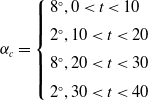 \begin{align}{\alpha _c} = \left\{ \begin{array}{l}{8^\circ },0 \lt t \lt 10\\[5pt]{2^\circ },10 \lt t \lt 20\\[5pt]{8^\circ },{\rm{ 2}}0 \lt t \lt 30\\[5pt]{2^\circ },30 \lt t \lt 40\end{array} \right.\end{align}
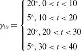 \begin{align}{\gamma _{Vc}} = \left\{ \begin{array}{l}{20^\circ },0 \lt t \lt 10\\[5pt]{5^\circ },10 \lt t \lt 20\\[5pt]{20^\circ },{\rm{ 2}}0 \lt t \lt 30\\[5pt]{5^\circ },30 \lt t \lt 40\end{array} \right.\end{align}
The second-order actuator
![]() $\dfrac{1}{{0.02{s^2} + 0.3s + 1}}$
is adopted to generate the span morphing rate
$\dfrac{1}{{0.02{s^2} + 0.3s + 1}}$
is adopted to generate the span morphing rate
![]() $\xi \in \left[ {0,1} \right]$
.
$\xi \in \left[ {0,1} \right]$
.
The hypersonic morphing vehicle is initialised as
![]() $\alpha \!\left( {{t_0}} \right) = 0$
,
$\alpha \!\left( {{t_0}} \right) = 0$
,
![]() $\beta \!\left( {{t_0}} \right) = 3$
,
$\beta \!\left( {{t_0}} \right) = 3$
,
![]() ${\gamma _V}\!\left( {{t_0}} \right) = 0$
,
${\gamma _V}\!\left( {{t_0}} \right) = 0$
,
![]() $V = 9Ma$
,
$V = 9Ma$
,
![]() $H = 30km$
and other states are zero at
$H = 30km$
and other states are zero at
![]() ${t_0} = 0$
.
${t_0} = 0$
.
Recalling the principles for the complete control system, which are conditions under (40), guidelines in (45) and (46), and requirements in theorem 1, (60)–(62), (72) and (74)–(75), the designed parameters are given as
![]() ${k_1} = 2$
,
${k_1} = 2$
,
![]() ${k_2} = 9.3$
,
${k_2} = 9.3$
,
![]() ${p_1} = 0.6$
,
${p_1} = 0.6$
,
![]() ${p_2} = 0.5$
,
${p_2} = 0.5$
,
![]() ${q_1} = 1.4$
and
${q_1} = 1.4$
and
![]() ${q_2} = 1.5$
for the sliding mode manifold.
${q_2} = 1.5$
for the sliding mode manifold.
![]() ${c_1} = 1.4$
,
${c_1} = 1.4$
,
![]() ${T_d} = {\rm{2}}{\rm{.5}}$
,
${T_d} = {\rm{2}}{\rm{.5}}$
,
![]() $m = 1.4$
,
$m = 1.4$
,
![]() $n = 0.6$
$n = 0.6$
![]() ${l_1} = {\rm{2}}$
,
${l_1} = {\rm{2}}$
,
![]() ${l_2} = {\rm{1}}$
,
${l_2} = {\rm{1}}$
,
![]() ${l_3} = {\rm{30}}$
,
${l_3} = {\rm{30}}$
,
![]() ${l_4} = 0.{\rm{5}}$
and
${l_4} = 0.{\rm{5}}$
and
![]() ${l_5} = {\rm{10}}$
for the controller.
${l_5} = {\rm{10}}$
for the controller.
![]() ${\lambda _{13}} = 0.1$
,
${\lambda _{13}} = 0.1$
,
![]() ${\lambda _{14}} = 1000$
,
${\lambda _{14}} = 1000$
,
![]() ${\lambda _{15}} = 12$
,
${\lambda _{15}} = 12$
,
![]() ${\lambda _{16}} = 0.001$
,
${\lambda _{16}} = 0.001$
,
![]() ${p_{0,2}} = 0.6$
,
${p_{0,2}} = 0.6$
,
![]() ${T_{1c}} = 3$
,
${T_{1c}} = 3$
,
![]() ${\theta _1} = 5$
,
${\theta _1} = 5$
,
![]() ${\mu _1} = 1.1$
,
${\mu _1} = 1.1$
,
![]() ${\lambda _{23}} = 0.1$
,
${\lambda _{23}} = 0.1$
,
![]() ${\lambda _{24}} = 4000$
,
${\lambda _{24}} = 4000$
,
![]() ${\lambda _{25}} = 3$
,
${\lambda _{25}} = 3$
,
![]() ${\lambda _{26}} = 0.0025$
,
${\lambda _{26}} = 0.0025$
,
![]() ${p_{0,2}} = 0.8$
,
${p_{0,2}} = 0.8$
,
![]() ${T_{2c}} = 4$
,
${T_{2c}} = 4$
,
![]() ${\theta _2} = 3.1$
and
${\theta _2} = 3.1$
and
![]() ${\mu _2} = 1.05$
for the fuzzy fixed-time disturbance observer. The fuzzy membership functions are
${\mu _2} = 1.05$
for the fuzzy fixed-time disturbance observer. The fuzzy membership functions are
![]() ${\Omega _1}\!\left( x \right) = {\left( {1 + {e^{3\!\left( {x + 0.5} \right)}}} \right)^{ - 1}}$
,
${\Omega _1}\!\left( x \right) = {\left( {1 + {e^{3\!\left( {x + 0.5} \right)}}} \right)^{ - 1}}$
,
![]() ${\Omega _2}\!\left( x \right) = {e^{ - {{\left( {x + 0.3} \right)}^2}}}$
,
${\Omega _2}\!\left( x \right) = {e^{ - {{\left( {x + 0.3} \right)}^2}}}$
,
![]() ${\Omega _3}\!\left( x \right) = {e^{ - {{\left( {x + 0.1} \right)}^2}}}$
,
${\Omega _3}\!\left( x \right) = {e^{ - {{\left( {x + 0.1} \right)}^2}}}$
,
![]() ${\Omega _4}\!\left( x \right) = {e^{ - {x^2}}}$
,
${\Omega _4}\!\left( x \right) = {e^{ - {x^2}}}$
,
![]() ${\Omega _5}\!\left( x \right) = {e^{ - {{\left( {x - 0.1} \right)}^2}}}$
,
${\Omega _5}\!\left( x \right) = {e^{ - {{\left( {x - 0.1} \right)}^2}}}$
,
![]() ${\Omega _6}\!\left( x \right) = {e^{ - {{\left( {x - 0.3} \right)}^2}}}$
and
${\Omega _6}\!\left( x \right) = {e^{ - {{\left( {x - 0.3} \right)}^2}}}$
and
![]() ${\Omega _7}\!\left( x \right) = {\left( {1 + {e^{ - 3\!\left( {x - 0.5} \right)}}} \right)^{ - 1}}$
. The methods to properly set the FLS is revealed in [Reference Zhang, Wang, Tang and Bao31].
${\Omega _7}\!\left( x \right) = {\left( {1 + {e^{ - 3\!\left( {x - 0.5} \right)}}} \right)^{ - 1}}$
. The methods to properly set the FLS is revealed in [Reference Zhang, Wang, Tang and Bao31].
5.1 Effectiveness verification
Time-varying commands to reveal the effectiveness of the controller are adopted. The corresponding curves are shown in Figs 2–4. The desired response curves are achieved with the help of the proposed control method under the two consecutive commands and morphing rate changes.
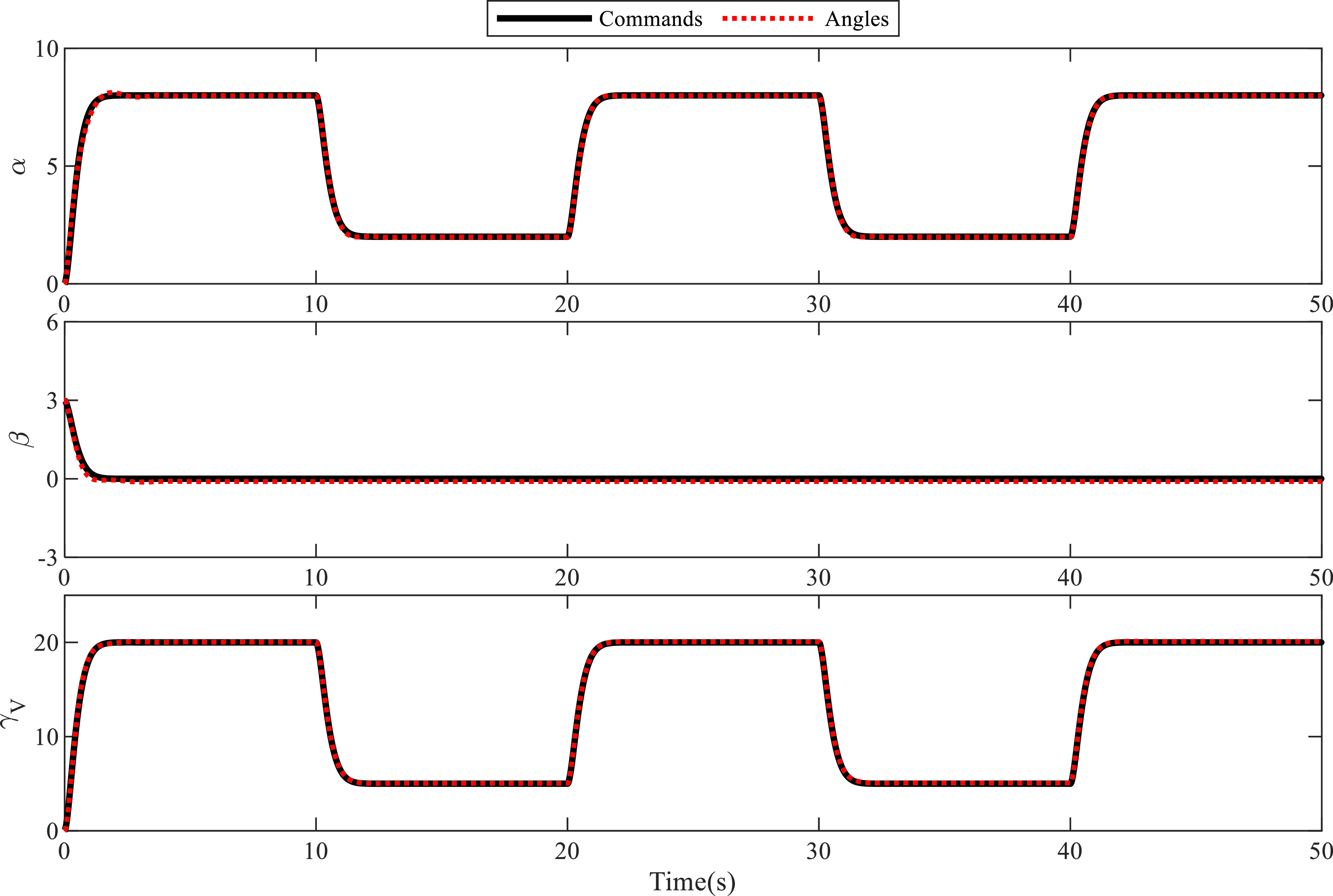
Figure 2. Commands and attitude angles.
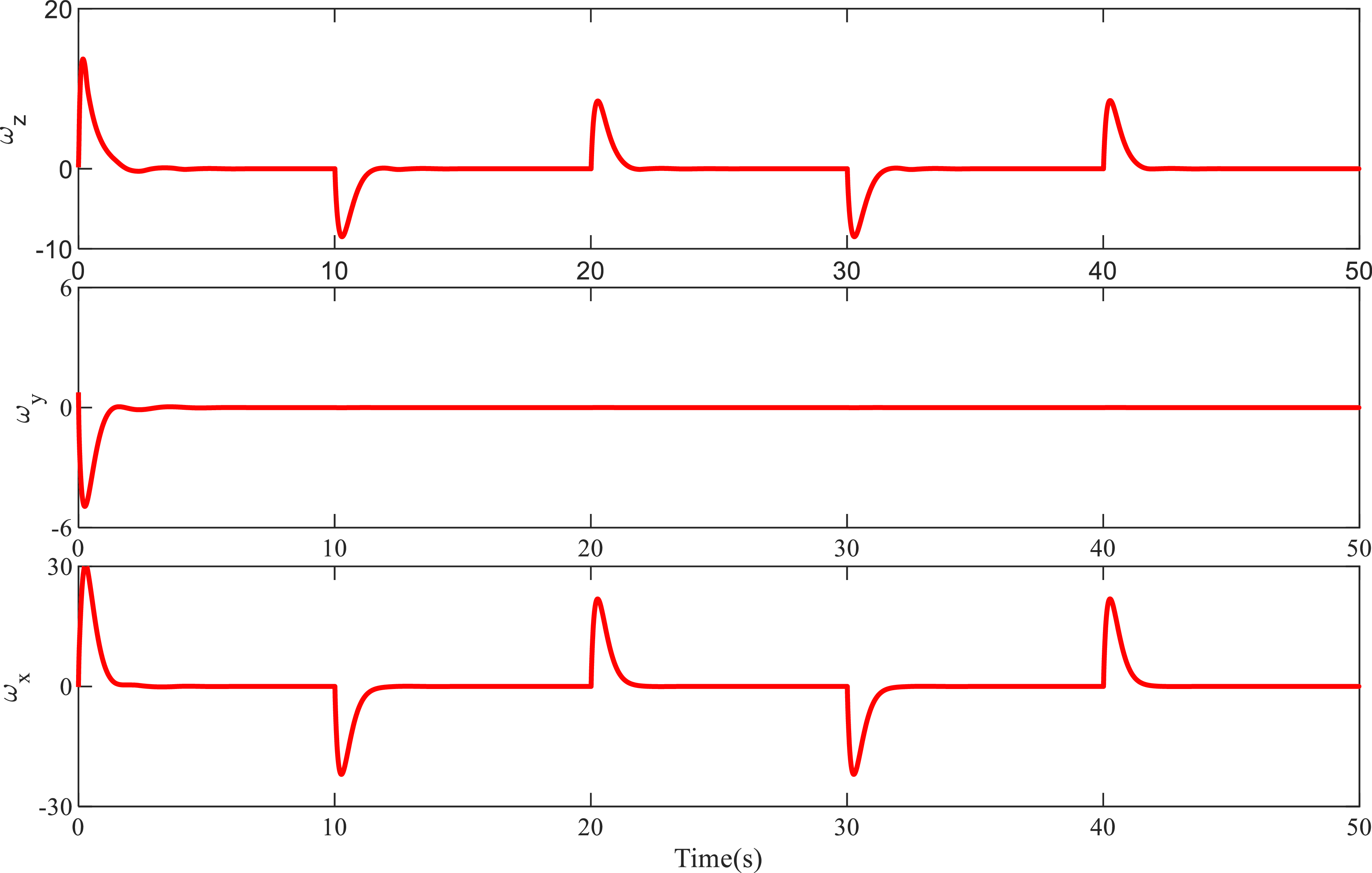
Figure 3. The curves of angular rates.
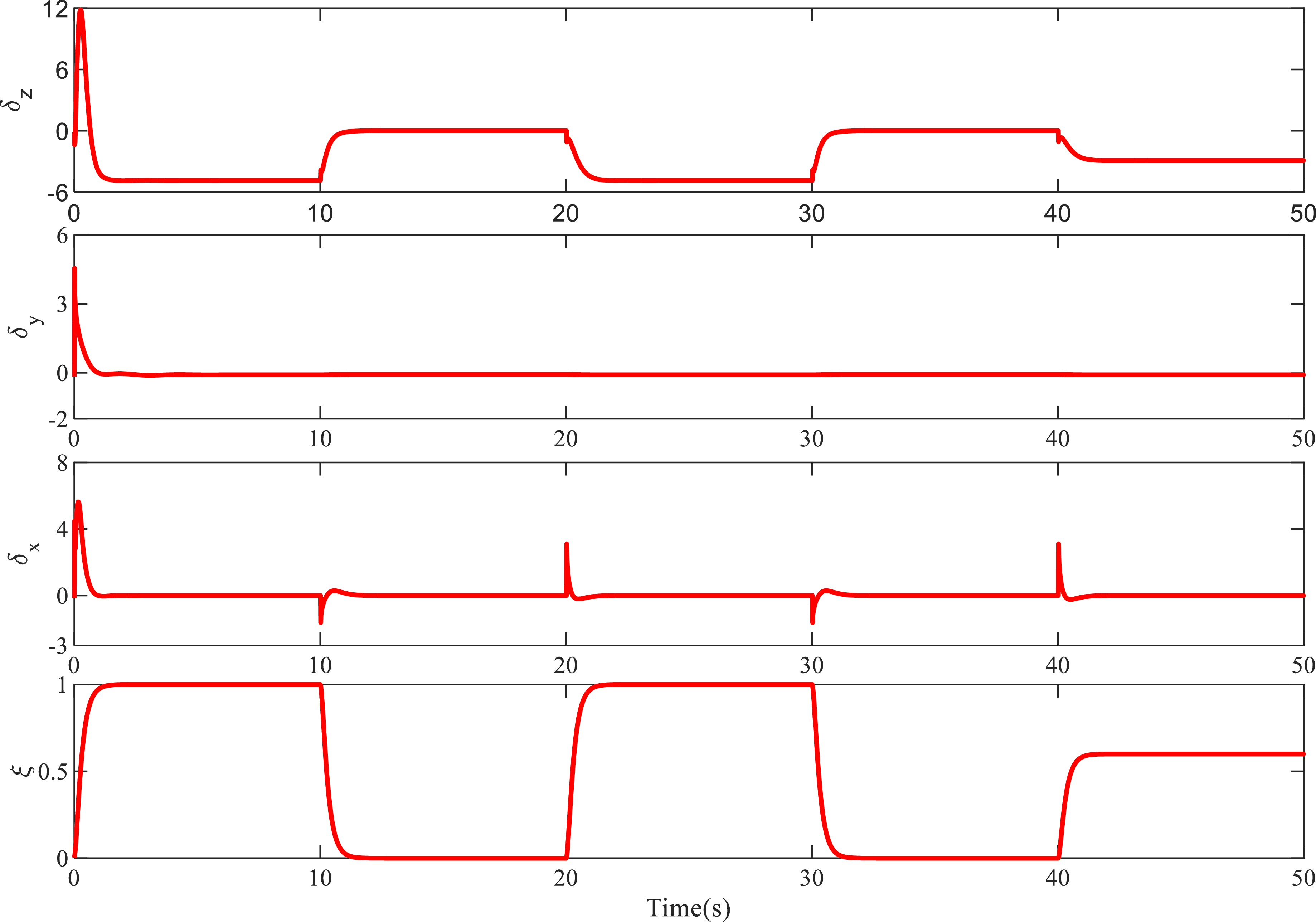
Figure 4. Control inputs and morphing rate.
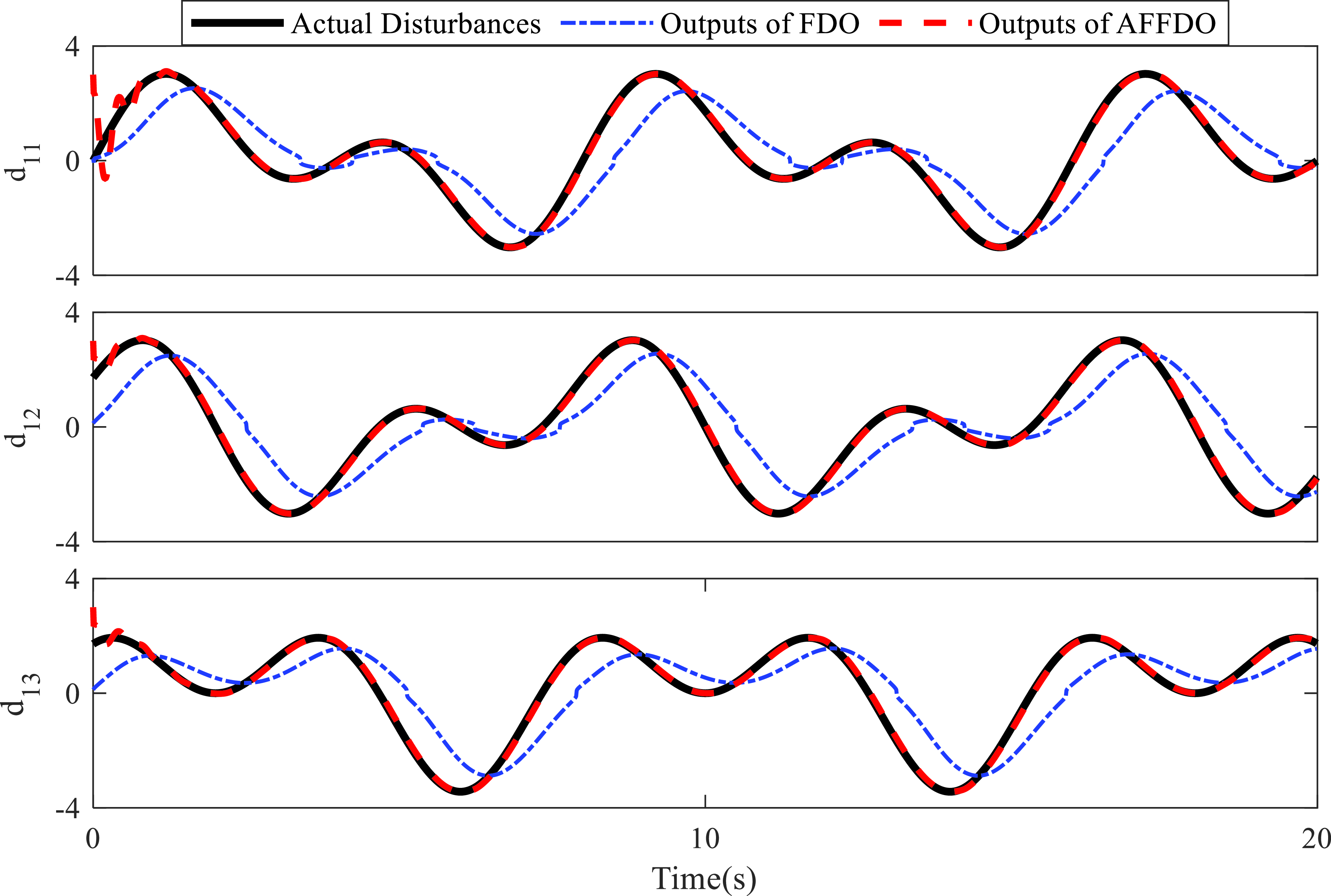
Figure 5. Mismatched disturbance estimations in case 1.
Figure 1 elaborates on the excellent tracking results of the states. All the attitude angles smoothly track the commands with 2s. Figure 2 reveals the curves of the angular rates. Figure 3 shows the control surfaces and the morphing rate. Since the span morphing influences the aerodynamic characteristic, the steady-state value of the controller changes. The results in this simulation illustrate the effectiveness of the proposed controller. All the angles can accurately track the reference commands within 2.5s when the HMV is flying in morphing processes. The states are continuous, and the curves of the controllers are acceptable. The varying steady value of
![]() ${\delta _z}$
implies the dramatic changes in aerodynamic properties.
${\delta _z}$
implies the dramatic changes in aerodynamic properties.
5.2 Comparison among different disturbance observers
The disturbance estimations are revealed in this simulation. Therefore, angles and morphing ratio are set to
![]() $\alpha = {2^ \circ }$
,
$\alpha = {2^ \circ }$
,
![]() $\beta = {0^ \circ }$
,
$\beta = {0^ \circ }$
,
![]() ${\gamma _V} = {0^ \circ }$
and
${\gamma _V} = {0^ \circ }$
and
![]() $\xi = 0$
. The conventional fixed-time disturbance observer and the parameters are obtained from the research [Reference Wang, Guo, Tang and Qi37]. Based on the literature [Reference Zhang, Wang, Tang and Bao31], three sets of disturbances are introduced. In case 1, the disturbances are
$\xi = 0$
. The conventional fixed-time disturbance observer and the parameters are obtained from the research [Reference Wang, Guo, Tang and Qi37]. Based on the literature [Reference Zhang, Wang, Tang and Bao31], three sets of disturbances are introduced. In case 1, the disturbances are
![]() ${{\boldsymbol{d}}_1} = 0.6{{\boldsymbol{\Delta }}_1}$
and
${{\boldsymbol{d}}_1} = 0.6{{\boldsymbol{\Delta }}_1}$
and
![]() ${{\boldsymbol{d}}_2} = 0.6{{\boldsymbol{\Delta }}_2}$
; In case 2, they are
${{\boldsymbol{d}}_2} = 0.6{{\boldsymbol{\Delta }}_2}$
; In case 2, they are
![]() ${{\boldsymbol{d}}_1} = 0.8{{\boldsymbol{\Delta }}_1}$
and
${{\boldsymbol{d}}_1} = 0.8{{\boldsymbol{\Delta }}_1}$
and
![]() ${{\boldsymbol{d}}_2} = 0.8{{\boldsymbol{\Delta }}_2}$
; we introduce
${{\boldsymbol{d}}_2} = 0.8{{\boldsymbol{\Delta }}_2}$
; we introduce
![]() ${{\boldsymbol{d}}_1} = {{\boldsymbol{\Delta }}_1}$
and
${{\boldsymbol{d}}_1} = {{\boldsymbol{\Delta }}_1}$
and
![]() ${{\boldsymbol{d}}_2} = {{\boldsymbol{\Delta }}_2}$
in case 3 with
${{\boldsymbol{d}}_2} = {{\boldsymbol{\Delta }}_2}$
in case 3 with
 \begin{align*}{{\boldsymbol{\Delta }}_1} = {1 \over {20}}\left[\begin{array}{l} {\sin 0.5\pi t} \\[5pt] {\sin 0.5\pi t} \\[5pt] {\cos 0.5\pi t} \\[5pt] \end{array}\right] + {1 \over {20}}\left[\begin{array}{l} {\sin 0.25\pi t} \\[5pt] {\cos 0.25\pi t} \\[5pt] {\sin 0.25\pi t} \\[5pt] \end{array}\right]rad/s\,{\rm{and}}\,\,\,\,{{\boldsymbol{\Delta }}_2} = 10{{\boldsymbol{d}}_1}{rad} /{s^2}\end{align*}
Figs 5–10 discloses that the estimation of the proposed AFFDO is better than the conventional FDO in the presence of mismatched and matched disturbances. By applying the designed AFFDO, the mismatched disturbances in three cases can be accurately estimated, which is helpful in disturbance compensation. It is announced that the proposed disturbance observer will provide outstanding disturbance estimations without the information on disturbance derivatives, which is necessary for the conventional FDO [Reference Wang, Guo, Tang and Qi37]. Moreover, since the settling time of the proposed methods can be easily pre-specified, the disturbance observer with better convergence performance is available.

Figure 6. Matched disturbance estimations in case 1.
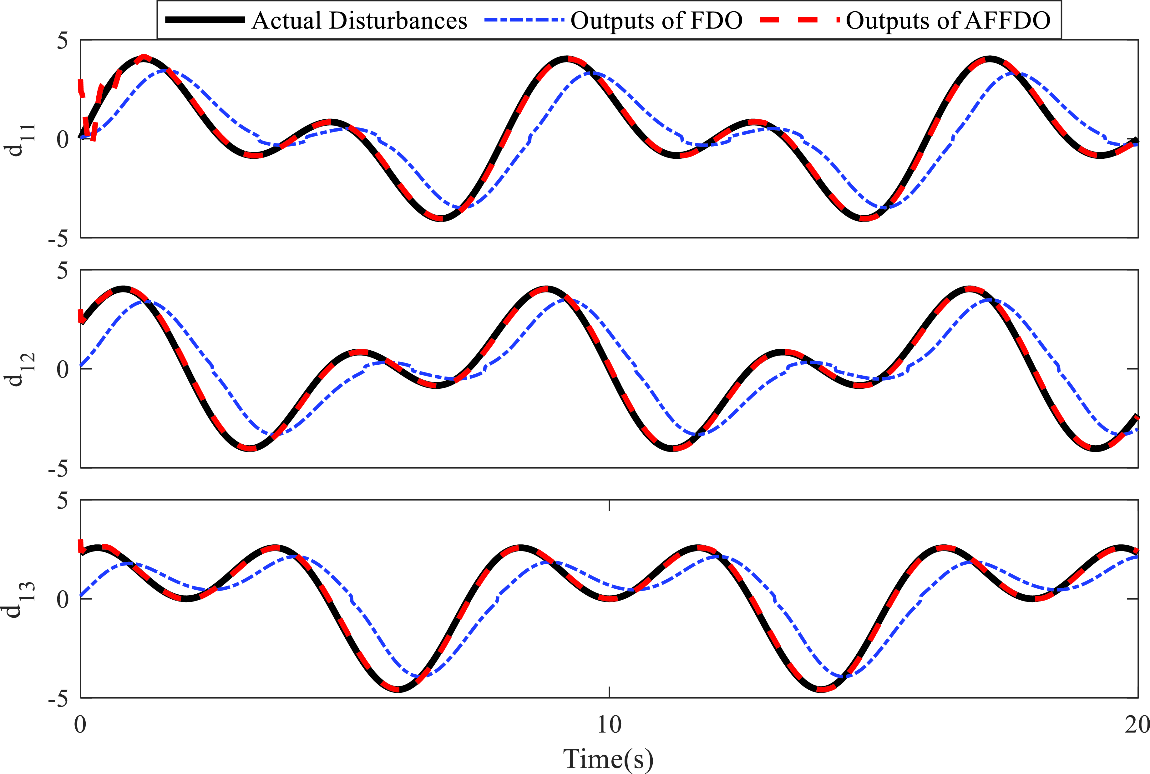
Figure 7. Mismatched disturbance estimations in case 2.
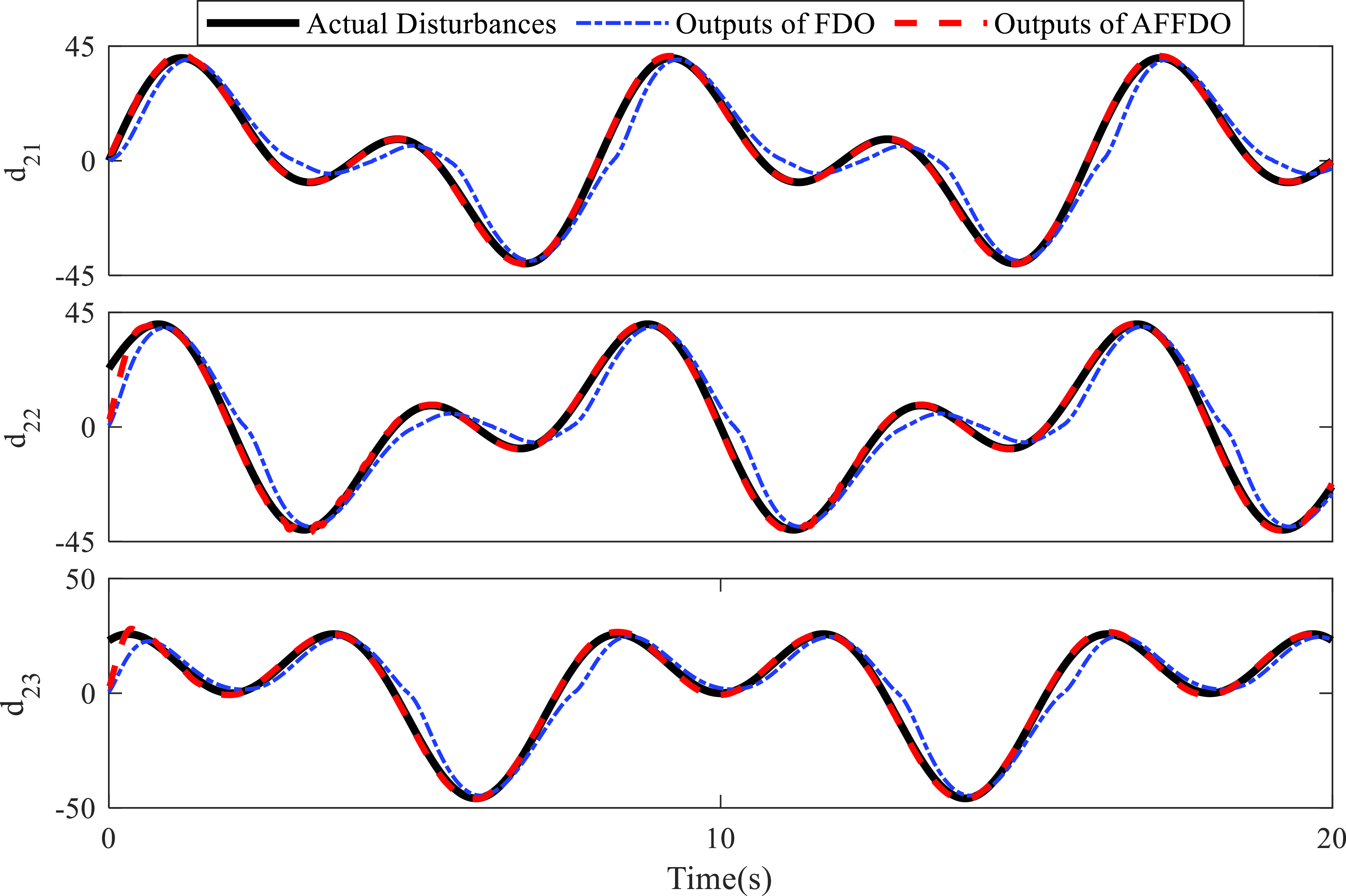
Figure 8. Matched disturbance estimations in case 2.
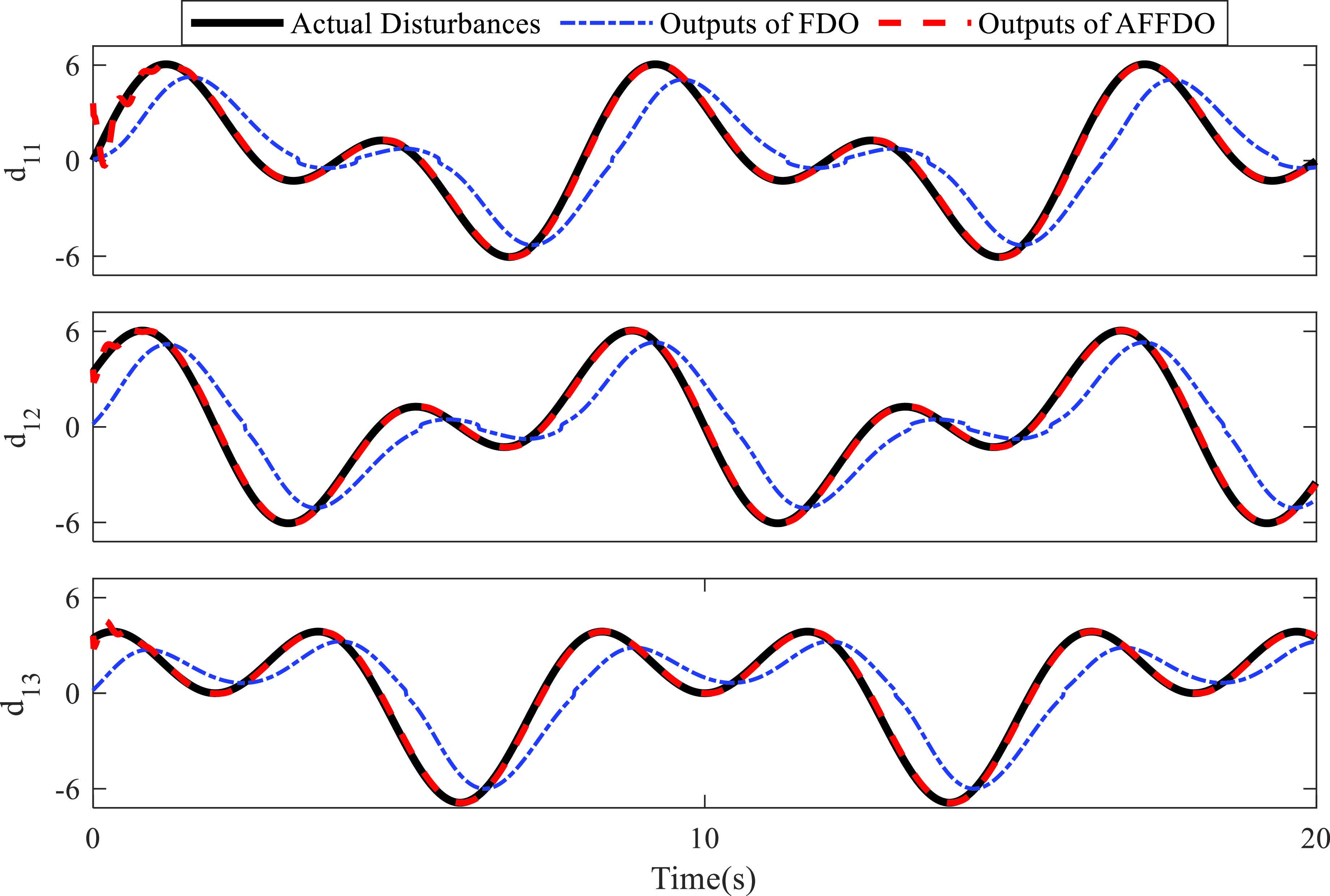
Figure 9. Mismatched disturbance estimations in case 3.

Figure 10. Matched disturbance estimations in case 3.
5.3 Disturbance compensation demonstration
From the previous simulation, the disturbance estimation performance could be verified. Since matched and mismatched disturbances are inevitable in the flight mission, it is necessary to offer an inspection for the controller. Now, we need to demonstrate the disturbance rejection. The proposed fixed-time control without/with the developed AFFDO is designed to test the performance. Figure. 11 shows that the anti-disturbance performance is obviously improved by introducing the proposed disturbance observer. Figures 12 and 13 show the angular rates, controller and morphing ratio. According to Figs 14 and 15, we can find that the disturbances are well estimated by the designed disturbance observer. Note that
![]() ${{\boldsymbol{d}}_1} = {{\boldsymbol{\Delta }}_1}$
and
${{\boldsymbol{d}}_1} = {{\boldsymbol{\Delta }}_1}$
and
![]() ${{\boldsymbol{d}}_2} = {{\boldsymbol{\Delta }}_2}$
are adopted in this simulation.
${{\boldsymbol{d}}_2} = {{\boldsymbol{\Delta }}_2}$
are adopted in this simulation.

Figure 11. Commands and attitude angles.

Figure 12. The curves of angular rates.
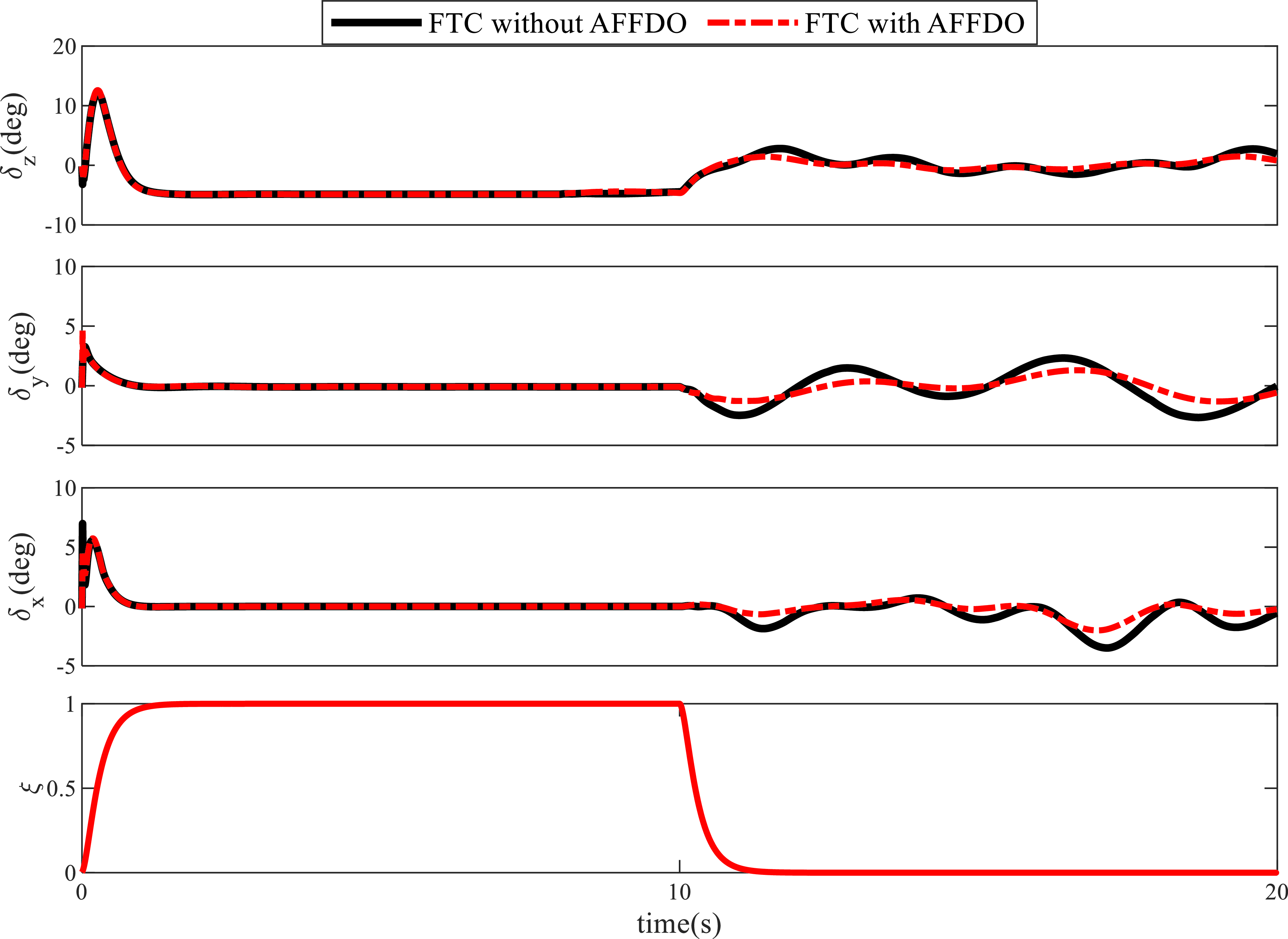
Figure 13. Control inputs and morphing rate.

Figure 14. Mismatched disturbance estimations.

Figure 15. Matched disturbance estimations.
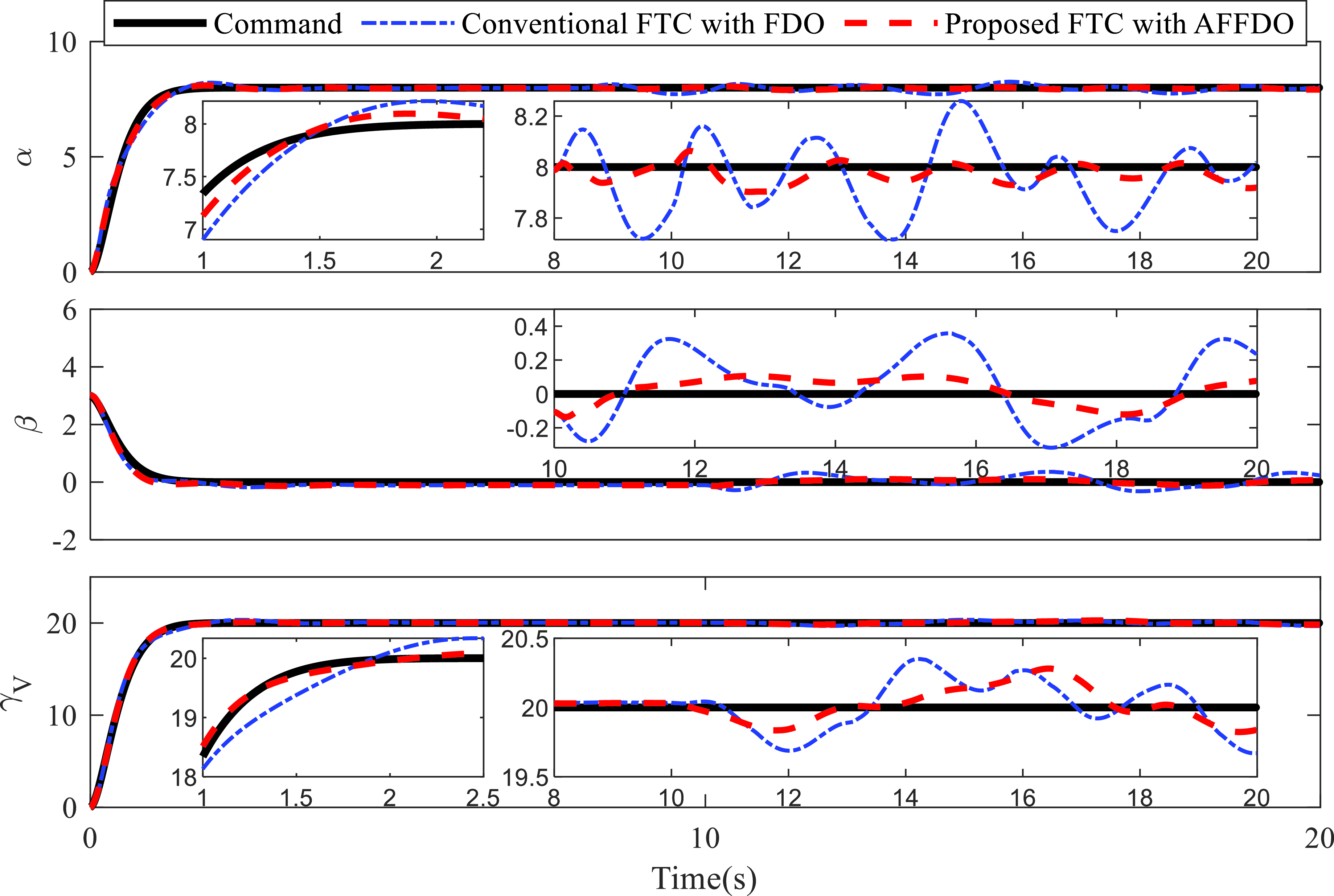
Figure 16. The commands and responses.
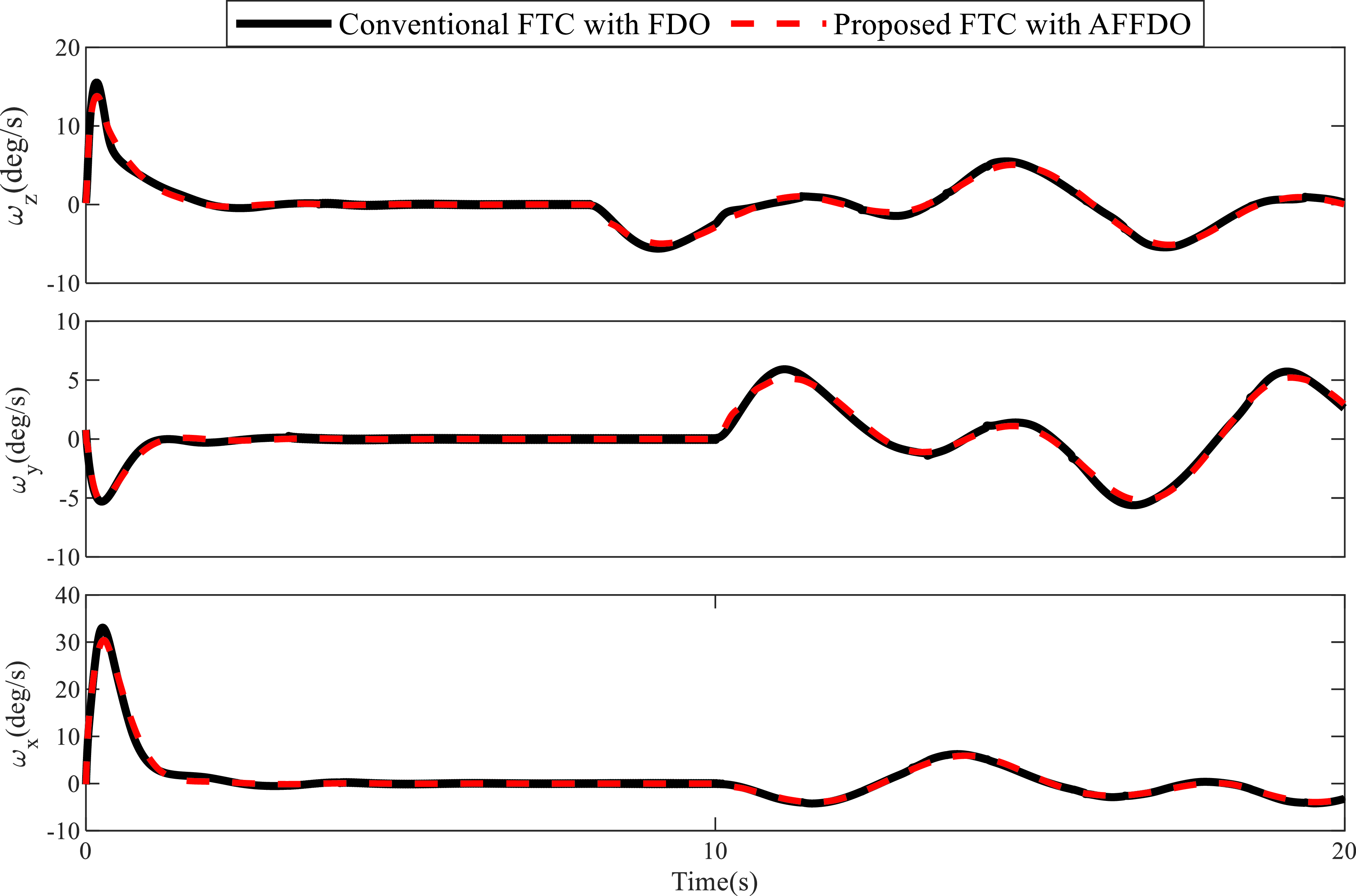
Figure 17. The angular rates.
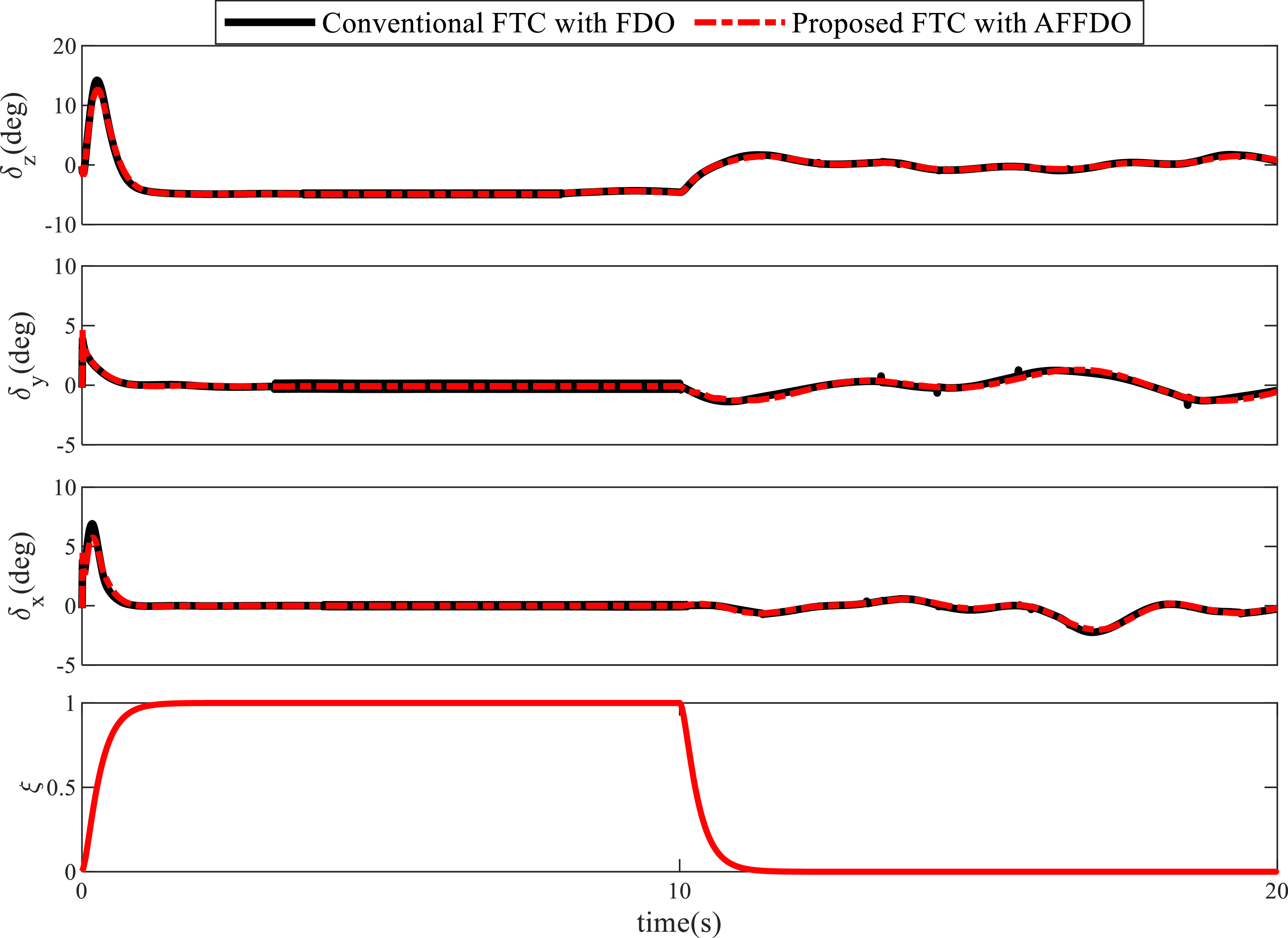
Figure 18. The control inputs and morphing ratio.
5.4 Comparison among different control methods
Researchers have proposed numerous control methods with different performances. However, for hypersonic morphing vehicles, the controller should have strong robustness and adaptation. The full control method in [Reference Wang, Guo, Tang and Qi37] is chosen to make the comparison, which is indicated by conventional FTC with FDO.
![]() ${d_{11}}$
and
${d_{11}}$
and
![]() ${d_{21}}$
start to make the impact at
${d_{21}}$
start to make the impact at
![]() $t = 8s$
, while the others affect the states from
$t = 8s$
, while the others affect the states from
![]() $t = 10s$
. The results are shown in Figs 16–20.
$t = 10s$
. The results are shown in Figs 16–20.

Figure 19. The mismatched disturbance estimations.

Figure 20. The matched disturbance estimations.
Figure 16 shows that the robustness of the proposed control method is better when the proposed strategy is compared with the method in [Reference Wang, Guo, Tang and Qi37]. The different levels of improvement of the tracking performance are obtained. Disturbance suppression is ensured by integrating the proposed fuzzy disturbance observer. The proposed control technique has more excellent anti-disturbance performance. Figures 17 and 18 show the corresponding angular rates and the control inputs. Figures 19 and 20 reveal the outputs from the disturbance observers, indicating the different disturbance estimations.
5.5 Control against of aerodynamic parameters perturbations
Since the wingspan morphing technique is introduced, hypersonic morphing vehicles cover a large flight envelop. Therefore, it is important to validate the uncertainties rejection performance. In comparison with the nominal case without any aerodynamic perturbance, the positive perturbance and negative perturbance scenarios are designed to demonstrate the anti-uncertainties performance of the proposed control method. The atmosphere density perturbance is set to
![]() $ \pm 20\% $
, while the aerodynamic force
$ \pm 20\% $
, while the aerodynamic force
![]() $\bar C_L^\alpha $
,
$\bar C_L^\alpha $
,
![]() $\bar C_D^\alpha $
,
$\bar C_D^\alpha $
,
![]() $\bar C_N^\beta $
and moment coefficients
$\bar C_N^\beta $
and moment coefficients
![]() $\bar m_x^{{\delta _x}},\bar m_y^{{\delta _y}},\bar m_z^{{\delta _z}}$
are perturbed by
$\bar m_x^{{\delta _x}},\bar m_y^{{\delta _y}},\bar m_z^{{\delta _z}}$
are perturbed by
![]() $ \pm 30\% $
. The morphing rate is same as the previous simulation.
$ \pm 30\% $
. The morphing rate is same as the previous simulation.

Figure 21. Commands and responses.
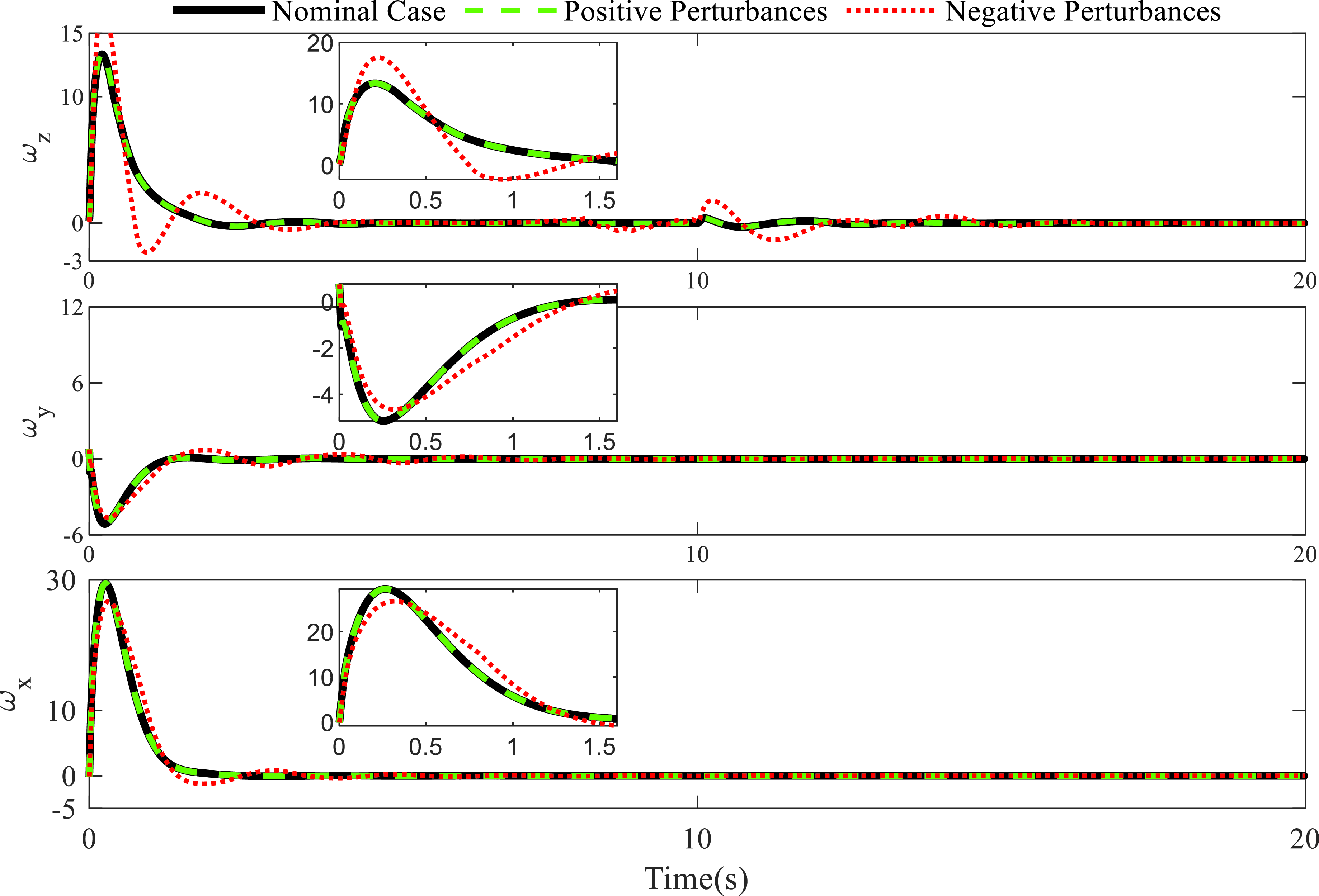
Figure 22. Angular rates.
The results are shown in Figs 21–23. Figure 21 reveals that the positive and negative perturbances impact the convergence procedure of the tracking error. However, all states can get rid of the influence of the different perturbances within 2s, which demonstrates the stability of the closed-loop HMV system. Figures 22 and 23 display the corresponding angular rates and the control inputs. In a word, a wide-range flight is achieved for hypersonic morphing vehicles without sacrificing tracking performance in the presence of aerodynamic perturbations.

Figure 23. Control inputs and morphing ratio.
6.0 Discussion
A high-accuracy flight control system for HMV has been developed by applying fixed-time control and fuzzy control. The developed fixed-time controller results in an explicit settling time than the traditional fixed-time control method. Moreover, disturbance suppression is achieved without any knowledge of the disturbance derivatives. Therefore, the anti-disturbance method could be available in engineering applications. The complete flight controller ensures fast and high-accuracy attitude tracking. The results of hypersonic flights in morphing phases match the theoretical findings.
It is necessary to reveal the limitations of the proposed method. The parameters of fuzzy memberships will impact the disturbance estimation. The designed disturbance observer with proper fuzzy memberships will adapt to various disturbances. Inappropriate will deteriorate the disturbance observation. Additionally, the application of the fuzzy logic system will require more computational resources.
Future work will focus on prescribed performance control for HMVs to enhance the flight control performance.
7.0 Conclusions
In this paper, the robust fixed-time controller is constructed to solve the tracking issue for an HMV with multisource uncertainties. The developed control method utilises a fixed-time control technique, homogeneous system theory, and fuzzy logic system to induce the controller. By using the adaptive fuzzy fixed-time disturbance observer, the influence of multisource uncertainties is ideally estimated and compensated. With the help of introducing the homogeneous degree concept, the tracking error converges in a fixed time after the convergence of the multivariable sliding mode variable. The proposed controller has achieved favorable performance in terms of robustness against time multisource uncertainties without the cost of sacrificing the control performance. The Lyapunov theory-based stability analysis is provided to prove the stability of the closed-loop system. The hypersonic morphing vehicle in the morphing phase is studied as the application. Three simulation cases show robustness against disturbance as well as dynamic uncertainties. Future work will consider the development of a prescribed performance controller for hypersonic morphing vehicles.
Funding sources
This work is supported by the National Natural Science Foundation of China Youth Fund (grant number 62003355).
Appendix A. Variables
Table A1. The indications in the model
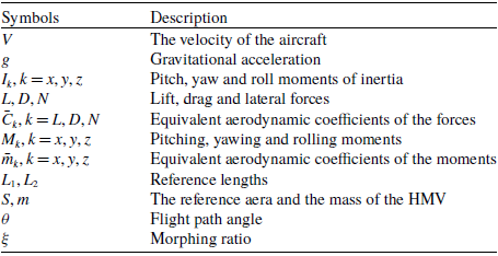
Table A2. The symbols in the control-oriented model

Table A3. The definitions in the sliding mode controller

Table A4. The symbols in the disturbance observer


