2.1 Notation and fundamental assumptions

We fix some notation that will be used throughout. Let k denote an algebraically closed field, and any category is additive, k-linear and essentially small. We deal with finite-dimensional abelian and triangulated categories of modules (resp., dg modules) over a finite-dimensional algebra (resp., a dg algebra). Whenever we define a subcategory, we mean that there is a fully faithful functor that we assume to be the embedding.

Given subcategories ${\mathcal A}_1,{\mathcal A}_2$ of an abelian or a triangulated category $\mathcal C$ , and a set of objects $\mathcal B$ , we define (usually omitting the subscript $\mathcal C$ )

We define $\langle \mathcal B\rangle $ depending on the context to be the abelian category generated by $\mathcal B$ , the thick triangulated category generated by $\mathcal B$ , the torsion-free class or the torsion class generated by $\mathcal B$ .

Let ${\mathcal A}$ be an abelian category. It is called a (finite) length category if any object $E\in {\mathcal A}$ admits a finite sequence of subobjects

$$\begin{align*}0=E_0\subset E_1 \subset \dots \subset E_m=E\end{align*}$$

such that all $E_i/E_{i-1}$ are simple. It is called finite if, moreover, it has finitely many simple objects. If an abelian category is finite, its Grothendieck group is generated by the isomorphism classes of its simples.

Let ${\mathcal D}$ be a triangulated category. For simplicity, we make the strong assumption that its Grothendieck group is a finite rank lattice $K({\mathcal D})\simeq \mathbb {Z}^{\oplus n}$ . This is not the general situation, though it will hold for the most relevant categories considered later. The main reason for such an hypothesis is to simplify the definition of a (multi-scale) stability condition.

The heart ${\mathcal A}$ of a bounded t-structure is an abelian category. The cohomological functor $H^0:{\mathcal D}\to {\mathcal A}$ realizes an isomorphism at the level of Grothendieck groups

$$\begin{align*}H^0_*:K({\mathcal A})\simeq K({\mathcal D}).\end{align*}$$

Moreover, a bounded t-structure is uniquely determined by its heart as $\mathcal P= \langle \mathcal {H}[i],i\geq 0\rangle $ . For this reason, we will speak about a t-structure or its heart interchangeably.

There is a partial order on hearts ${\mathcal A}_1\le {\mathcal A}_2$ defined by $\mathcal P_1\supset \mathcal P_2$ , or equivalently, $\mathcal P_1^\perp \supset \mathcal P_2^\perp $ . A heart $\mathcal {H}$ will be called intermediate with respect to a fixed heart ${\mathcal A}$ if ${\mathcal A} \leq \mathcal {H} \leq {\mathcal A}[1]$ .

2.2 Torsion pairs and tilting

A torsion pair for an abelian category ${\mathcal A}$ consists of a pair $(\mathcal {T},\mathcal {F})$ of full additive subcategories of ${\mathcal A}$ called torsion class and torsion-free class, such that ${\mathcal A}=\mathcal {T}\perp \mathcal {F}$ . In other words, a torsion pair mimics a bounded t-structure at abelian level. In fact, a torsion pair in the heart of a bounded t-structure ${\mathcal A}$ in a ${\mathcal D}$ defines new bounded t-structures with hearts

$$\begin{align*}\mu_{\mathcal{F}}^\sharp{\mathcal A}:= \mathcal{T} \perp_{\mathcal D} \mathcal{F}[1], \quad \mu_{\mathcal{T}}^\flat{\mathcal A}:=\mathcal{F}\perp_{\mathcal D} \mathcal{T}[-1]. \end{align*}$$

They are called, respectively, the forward tilt at $\mathcal {F}$ (resp. backward tilt at $\mathcal {T}$ ), [Reference Happel, Reiten and SmaløHRS96]. They are related by $\mu ^\sharp _{\mathcal {T}[-1]} \mu ^\flat _{\mathcal {T}}{\mathcal A}={\mathcal A}$ and $\mu ^\flat _{\mathcal {F}[1]}\mu ^\sharp _{\mathcal {F}}{\mathcal A} = {\mathcal A}$ . The forward tilt of ${\mathcal A}$ at a torsion-free class is intermediate with respect to ${\mathcal A}$ ; the backward tilt of ${\mathcal A}$ at a torsion class is intermediate with respect to ${\mathcal A}[-1]$ .

In a finite abelian category, torsion and torsion-free classes are closed under extensions and are characterized by being closed under quotients and subobjects, respectively. This implies that any Serre subcategory is both torsion and torsion-free class. When we tilt at a torsion(-free) class $\langle S\rangle $ generated by a simple object S, we speak about a simple tilt, and we simplify the notation to $\mu ^\sharp _S{\mathcal A}$ and $\mu ^\flat _S{\mathcal A}$ . Suppose ${\mathcal A}$ is a finite heart with simple objects $\operatorname {Sim}({\mathcal A}):=\{S_1,\dots , S_n\}$ , which are rigid (i.e., have no nontrivial self-extensions), and let $S\in \operatorname {Sim}({\mathcal A})$ . Then

$$\begin{align*}\begin{aligned} \operatorname{Sim} \mu^\sharp{\mathcal A} &= \{S[1]\}\cup \{\operatorname{Cone}\big(S\stackrel{ev}{\to}S[1]\otimes \operatorname{Ext}^1(T,S)^*\big)[-1], \ S\neq T \in\operatorname{Sim}{\mathcal A}\}\\ \operatorname{Sim} \mu^\flat{\mathcal A} &= \{S[-1]\}\cup \{\operatorname{Cone}\big(S[-1]\otimes \operatorname{Ext}^1(S,T)\stackrel{ev}{\to} T), \ S\neq T \in\operatorname{Sim}{\mathcal A}\}.\, \end{aligned}\end{align*}$$

See, for example, [Reference King and QiuKQ15]. Note also that the simple tilting of a finite heart in ${\mathcal D}$ is another finite heart. In some cases, tilting at a torsion (or torsion-free) class can be decomposed into a finite sequence of simple tilts.

2.3 Bridgeland stability conditions

Recall from [Reference BridgelandBri07] that a stability condition $\sigma $ on a triangulated category ${\mathcal D}$ is a pair $\sigma = ({\mathcal A},Z)$ , consisting of the heart of a bounded t-structure ${\mathcal A}$ , together with a central charge (i.e., a group homomorphism that maps the class of nonzero elements in ${\mathcal A}$ to the semi-closed half plane $\overline {\mathbb {H}}:=\{re^{\pi i \theta }\in {\mathbb R} | r\in {\mathbb R}_{>0},\ 0<\theta \leq 1\}$ and that satisfies the support property and Harder-Narasimhan condition of loc. cit). We fix a finite rank lattice K and a surjective morphism $\nu : K({\mathcal A})\to K$ and require that Z factors through $\nu $ . In the case , we require that $K = K({\mathcal A})$ and .

We use that stability conditions can equivalently be specified as a $\sigma = (\mathcal {P}, Z)$ using a central charge and a slicing, compatible in the sense that $E\in \mathcal P(\phi )$ implies $Z([E])=m\exp (\pi i \phi )$ for some positive $m\in \mathbb {R}$ .

An object $E\in {\mathcal D}$ is called $\sigma $ -semistable if $E\in \mathcal P(\phi )$ for some $\phi \in \mathbb {R}$ . It is called $\sigma $ -stable if it is simple in $\mathcal P(\phi )$ . This notion makes sense because any subcategory $\mathcal P(\phi )$ is abelian if $\mathcal P=\{\mathcal P(\phi )\}_{\phi \in \mathbb {R}}$ is a slicing compatible with .

Let $\lambda \in \mathbb {C}$ , and suppose $0 < \epsilon = \Re (\lambda ) \leq 1$ . We observe, and will use later, that $\sigma $ -semistable objects X in the heart ${\mathcal A}$ (equivalently Z-semistable objects) with $1-\epsilon \leq \phi (X) <(\leq ) 1$ and those with $0<\phi (X)\leq (<)1-\epsilon $ , for $\epsilon \in (0,1)$ , form a torsion pair $(\mathcal {T}_\lambda ,\mathcal {F}_\lambda )$ in ${\mathcal A}$ due to the Harder-Narasimhan condition.

The space of stability conditions is a complex manifold . There are two natural commuting actions:

• ○ a left action by $\mathbb {C}$ , by rescaling the central charge and tilting the heart, if $0 < \Re (\lambda ) \leq 1$ ,

  $$\begin{align*}\lambda \cdot ({\mathcal A},Z) \;=\;(\mu^\sharp_{\mathcal{F}_\lambda} {\mathcal A},e^{-\pi i \lambda} Z)\,,\end{align*}$$

• ○ and a right action by via pullback,

  $$\begin{align*}\Phi.({\mathcal A},Z) \;=\;\big(\Phi {\mathcal A},Z\circ [\Phi]^{-1})\big),\end{align*}$$
  where $[\Phi ]$ is the map induced by $\Phi $ on $K({\mathcal D})$ .

In particular, the shift $[1]$ acts as $\lambda =1$ . Note that the $\mathbb {C}$ -action does not change the notion of semistability and stability.

We denote by a connected component, specified by the context. The stability manifold is tiled into subsets of stability conditions supported on the heart ${\mathcal A}$ . The component is called finite type if it is the union of over finite hearts. It is called of tame type if the $\mathbb {C}$ -orbits of for all finite type hearts cover .

We let be the subgroup of consisting on autoequivalences of $\mathcal {D}$ that preserve the component , and we define the subgroup of negligible autoequivalences (i.e., those that act trivially on ). We use fancy fonts like

(2)

to denote the quotient groups by negligible autoequivalences. It is the quotient spaces by these actions that we want to compactify.

2.4 Quivers with potential, module and Ginzburg categories

In this paper, $(Q,W)$ is a quiver $Q=(Q_0,Q_1,s,t)$ with potential W (i.e., a formal sum of cycles) up to right-equivalence; see [Reference Derksen, Weyman and ZelevinskyDWZ08; Reference Keller and YangKY11] for standard results. We assume that $(Q,W)$ has no loops and no 2-cycles, that the set of vertices $Q_0$ and the set of arrows $Q_1$ are finite, and that the potential defines a bilateral ideal $\partial W=\langle \partial _a W \mid a\in Q_1\rangle \subset k Q$ such that the Jacobian algebra,

$$\begin{align*}\mathcal J(Q,W) := \widehat {k Q}/\partial W,\end{align*}$$

obtained by quotienting the completed path algebra by the ideal defined by the potential, is finite dimensional. Note that in our case of interest, $\widehat {k Q}/\partial W =k Q/\partial W$ . For a ring $\mathcal J$ , we denote by $\operatorname {Mod} \mathcal J$ the abelian category of left modules and by $\operatorname {mod} \mathcal J$ the abelian category of finitely generated left modules. The category $\operatorname {mod} \mathcal J(Q,W)$ is finite with simple objects $\operatorname {Sim}(\operatorname {mod} \mathcal J(Q,W))=\{S_1,\dots , S_n\}$ , where $n=|Q_0|$ .

If $I\subset Q_0$ is a collection of vertices of $(Q,W)$ , by $(Q_I,W_I)$ , we mean the restriction of $(Q,W)$ to I. It is another finite quiver with potential, possibly disconnected, defined by $(Q_I)_0=I$ , $(Q_I)_1=\left \{a:i\to j\in Q_1\mid i,j\in I\right \}$ , and with source, tail functions and potential obtained by restriction from $(Q,W)$ to I. We call it a (full) subquiver. The complement of I in $Q_0$ will be denoted $I^c$ .

The mutation of a quiver with potential $(Q,W)$ at a vertex i is an operation that produces another quiver with the same set of vertices and a new set of arrows and a new potential, defined as follows. From $Q_1$ , keep all arrows not incident to i; replace any arrow a with either $s(a)$ or $t(a)$ equal to i with its opposite; add an arrow $[ab]:k_1\to k_2$ for any pair of consecutive arrows $a:k_1\to i$ and $b:i\to k_2$ ; finally, remove any two-cycles. The new potential is the formal sum of W and $\sum _{a,b\in Q_1}[ab]b^*a^*$ .

The Ginzburg algebra of $(Q,W)$ is a dg algebra denoted $\Gamma (Q,W)$ and introduced in [Reference GinzburgGin06; Reference Keller and YangKY11]. It does not depend on the mutation class of a quiver with potential.

Once we fixed $(Q,W)$ and $I\subset Q_0$ , we write $\mathcal J=\mathcal J(Q,W)$ , $\Gamma =\Gamma (Q,W)$ , and $\mathcal J_I=\mathcal J(Q_I,W_I)$ , $\Gamma _I=\Gamma (Q_I,W_I)$ . We have the following inclusion of triangulated categories, [Reference Keller and YangKY11]

$$\begin{align*}\operatorname{pvd}(\Gamma) \subset \operatorname{per}(\Gamma) \subset {\mathcal D}(\Gamma).\end{align*}$$

It is proven in [Reference Keller and YangKY11] that the standard t-structure with heart $\operatorname {Mod}\mathcal J$ in the derived category ${\mathcal D}(\Gamma )$ restricts to $\operatorname {per}(\Gamma )$ and $\operatorname {pvd}(\Gamma )$ , on which it defines a bounded t-structure with heart $\mod \mathcal J$ , that we call standard as well.

The perfectly valued derived category of the Ginzburg algebra of a quiver with potential is 3-Calabi-Yau, which means that for any objects $E,F\in \operatorname {pvd}(\Gamma )$ , there is a natural isomorphism of k-vector spaces . Moreover, the simple objects in the standard heart $\mod \mathcal J$ are spherical in $\operatorname {pvd}(\Gamma )$ ; see [Reference KellerKel11, Lemma 4.4] and [Reference King and QiuKQ15, Corollary 8.5].

If two quivers with potential $(Q,W)$ and $(Q',W')$ are related by mutations, then ${\mathcal D}(\Gamma (Q,W))\simeq {\mathcal D}(\Gamma (Q',W'))$ and $\operatorname {pvd}(\Gamma (Q,W))\simeq \operatorname {pvd}(\Gamma (Q',W'))$ . Therefore, $\operatorname {mod}\mathcal J(Q',W')$ is viewed as another heart of bounded t-structure of $\operatorname {pvd}\Gamma (Q,W)$ . We recall that, in general, not all bounded t-structures have this shape.

It is clear that any property of $\operatorname {pvd}(\Gamma )$ and $\operatorname {mod}(\mathcal J)$ also holds for $\operatorname {pvd}(\Gamma _I)$ and $\operatorname {mod} \mathcal J_I$ .

As explained in [Reference Kalck and YangKY18], the Ginzburg algebra $\Gamma _I$ is isomorphic to $\Gamma /\Gamma e \Gamma $ , where $e=\sum _{i\in I^c}e_i$ is the idempotent in $\Gamma $ associated to the complement $I^c= Q_0\setminus I$ . However, the dg algebra $e\Gamma e$ is the endomorphism algebra of the projective module $\Gamma e = \sum _{i\in I^c}\Gamma e_i$ in ${\mathcal D}(\Gamma )$ , and the Verdier quotient ${\mathcal D}(\Gamma )/{\mathcal D}(\Gamma _I)$ coincides with ${\mathcal D}(e\Gamma e)$ . Similarly, $\mathcal J_I=\mathcal J/\mathcal J e \mathcal J$ and the quotient perfectly valued and abelian categories that will be relevant in the rest of the paper are $\operatorname {pvd} e\Gamma e$ and $\operatorname {mod} e\mathcal J e$ :

The last line is part of a recollement of abelian categories, described, for instance, in [Reference PsaroudakisPsa18].

In the rest of the paper, we let

• ○ ${\mathcal D}_Q^3$ be the 3-Calabi-Yau triangulated category $\operatorname {pvd}\Gamma (Q,W)$ .

The case of primary interest will be quivers of type $A_n$ – that is, that can be obtained with by finite sequence of mutations from the quiver

Any restriction of a quiver of type $A_n$ is a union of quivers of type $A_m$ ’s.

Given an $A_n$ -configuration, and the abelian category $\operatorname {mod} \mathcal J(A_n)$ , we denote by $S_i$ the simple module associated with the vertex i. For $i\leq k$ , we denote by $S_{i...k}$ the $\mathcal J(A_n)$ -module defined inductively as the indecomposable fitting into the short exact sequence

(3) $$ \begin{align} 0 \rightarrow S_{k+1} \rightarrow S_{i\dots (k+1)} \rightarrow S_{i\dots k} \rightarrow 0. \end{align} $$

The $S_{i\dots k}$ , are the projective resolutions $P_i$ of $S_i$ in the abelian subcategory $\langle S_i,\dots , S_{k}\rangle $ which is of $A_{(k-i)}$ -type by construction.

3.1 The stability manifold of a decorated marked surface

A natural way to construct quivers is from triangulations of surfaces, and we will use this formalism to keep track of connected components of stability spaces and later the multi-scale stabilty conditions.

A marked surface $\mathbf {S}=(\mathbf {S},{\mathbb M},\mathbb P)$ consists of a connected bordered differentiable surface with a fixed orientation, with a finite set ${\mathbb M}=\{M_i\}_{i=1}^b$ of marked points on the boundary $\partial \mathbf {S}=\bigcup _{i=1}^b \partial _i$ , and with a finite set $\mathbb P=\{p_j\}_{j=1}^p$ of punctures in its interior $\mathbf {S}^\circ =\mathbf {S}-\partial \mathbf {S}$ , such that each connected component of $\partial \mathbf {S}$ contains at least one marked point.

A decorated marked surface ${\mathbf {S}}_\Delta $ (abbreviated as DMS) is obtained from a marked surface $\mathbf {S}$ by decorating it with a set $\Delta = \{z_i\}_{i=1}^r$ of points in the surface interior $\mathbf {S}^\circ $ . These points are called finite critical points or finite singularities.

An open arc is an (isotopty class of) curve $\gamma \colon I\to {\mathbf {S}}_\Delta $ such that its interior is in ${\mathbf {S}}_\Delta ^\circ \setminus \Delta $ and its endpoints are in the set of marked points ${\mathbb M}$ . An (open) arc system $\{\gamma _i\}$ is a collection of open arcs on ${\mathbf {S}}_\Delta $ such that there is no (self-)intersection between any of them in ${\mathbf {S}}_\Delta ^\circ \setminus \Delta $ . A triangulation ${\mathbb T}$ of ${\mathbf {S}}_\Delta $ is a maximal arc system of open arcs, which, in fact, divide ${\mathbf {S}}_\Delta $ into triangles.

The quiver $Q_{\mathbb T}$ with potential $W_{\mathbb T}$ associated to a triangulation ${\mathbb T}$ is constructed as follows. The vertices correspond to the open arcs in ${\mathbb T}$ , the arrows of $Q_{\mathbb T}$ correspond to oriented intersection between open arcs in ${\mathbb T}$ , so that there is a 3-cycle in $Q_{\mathbb T}$ locally in each triangle, and the potential $W_{\mathbb T}$ is the sum of all such $3$ -cycles.

For a fixed initial triangulation ${\mathbb T}_0$ , we denote by $\Gamma _{{\mathbb T}_0} = \Gamma (Q_{{\mathbb T}_0}, W_{{\mathbb T}_0})$ the Ginzburg algebra associated with the quiver associated with ${\mathbb T}_0$ we let ${\mathcal D}^3_{Q_{{\mathbb T}_0}} = \operatorname {pvd}(\Gamma _{{\mathbb T}_0})$ or simply $\mathcal {D}^{3}_{Q}$ the corresponding $CY_3$ -category. Finally, we define to be the connected component of the space of Bridgeland stability conditions on $\mathcal {D}^{3}_{Q}$ containing stability conditions supported on the standard heart ${\mathcal H}_0$ of $Q_{{\mathbb T}_0}$ .

In this paper, we fix throughout a DMS $\mathbf {S}$ of type $A_n$ . It is a disc with $b=1$ boundary component, which has $n+3$ marked points, $r= n+1$ finite critical points in its interior, and no punctures. We use this reference surface and a reference triangulation on it to define the component . Recall from [Reference Bridgeland and SmithBS15, Theorem 9.9 and Section 12.1] that the subgroup preserving a connected component of is an extension of $\mathbb {Z}/(n+3)\mathbb {Z}$ by the spherical twist group $\operatorname {ST}(A_n)$ .

In this language, the main theorem of Bridgeland-Smith (for a general $CY_3$ -quiver category $\mathcal {D}^{3}_{Q}$ associated with a triangulation of ${\mathbf {S}}_\Delta $ , see [Reference Bridgeland and SmithBS15] for the excluded cases) reads:

Theorem 3.1 [Reference Bridgeland and SmithBS15; Reference King and QiuKQ20]

There is an isomorphism of complex manifolds

(4)

This map K is equivariant with respect to the action of the mapping class group $\operatorname {MCG}(\mathbf {S}_{\Delta })$ on the domain and of the automorphism group on the range. These groups act properly discontinuously on domain, resp. range.

Here, $\operatorname {FQuad}^\circ (\mathbf {S}_{\Delta })$ is a space of framed quadratic differentials with simple zeros at $\Delta $ , whose definition we recall along with the examples in Section 6. Its generalization to nonsimple zeros motivates the notion of collapse and the use of quotient categories, which we recall in Section 3.2.

As a technical tool, we introduce the exchange graph $\operatorname {EG}({\mathbf {S}}_\Delta )$ , the directed graph whose vertices are the triangulations of ${\mathbf {S}}_\Delta $ and whose edges are given by (forward) flips of the triangulation. The exchange graph $\operatorname {EG}({\mathcal D})$ of a triangulated category is the directed graph whose vertices are the finite hearts and whose edges are given by forward tilts at simples in the heart. We denote by $\operatorname {EG}^\circ ({\mathbf {S}}_\Delta )$ the connected component containing the initial triangulation ${\mathbb T}_0$ and by $\operatorname {EG}^\circ (\mathcal {D}^{3}_{Q})$ the connected component corresponding to the standard heart $\mod \mathcal J(Q_{{\mathbb T}_0}, W_{{\mathbb T}_0})$ . A key step in the proof of Theorem 3.1 is the isomorphism

(5) $$ \begin{align} \operatorname{EG}^\circ({\mathbf{S}}_\Delta) \,\cong\, \operatorname{EG}^\circ(\mathcal{D}^{3}_{Q}) \end{align} $$

of exchange graphs.

3.2 Stability manifolds of certain quotient categories

Higher order zeros are modeled by the collapse of a subsurface $\Sigma \subset {\mathbf {S}}_\Delta $ in a DMS. We use this to deduce information on certain components of the stability manifold of the quotient categories $\mathcal {D}^{3}_{Q} / {\mathcal {D}^3_{Q_I}}$ . We decompose $\Sigma $ into connected components $\Sigma _i$ , and we provide each boundary component of $\Sigma _i$ with an integer enhancement $\kappa _{ij}$ . To match the hypothesis with [Reference Barbieri, Möller, Qiu and SoBMQS22], we suppose throughout that $\kappa _{ij} \geq 3$ and consider $\Sigma $ as a marked surface with $\kappa _{ij}$ points on each boundary component.

To topologically formalize the collapse of $\Sigma $ , we define a weighted DMS (wDMS for short) to be a DMS with a weight function $\mathbf {w}: \Delta \to \mathbb {Z}_{\geq -1}$ , where the total weight is required to be $||\mathbf {w}|| = 4g-4 + |{\mathbb M}|+2b$ . Contracting $\Sigma \subset {\mathbf {S}}_\Delta $ and replacing each boundary component by a decoration point in $\Delta $ with weight $\mathbf {w}_{ij} = \kappa _{ij}-2$ defines a wDMS that we usually denote by $\overline {{\mathbf {S}}}_{\mathbf {w}}$ . In the sequel (as in [Reference Barbieri, Möller, Qiu and SoBMQS22]), we restrict to the case of no punctures $p=0$ , no unmarked boundary components and $\mathbf {w}: \Delta \to \mathbb {Z}_{\geq 1}$ .

To categorify the collapse, we homotope the initial triangulation ${\mathbb T}_0$ such that the arcs intersect the boundary of $\Sigma $ in the marked points and such that ${\mathbb T}_0|_\Sigma $ is a triangulation of this subsurface. In this way, $\Sigma $ becomes a DMS with a triangulation, and we may form the $CY_3$ -category ${\mathcal D}_3(\Sigma )$ . We define the Verdier quotient category

(6) $$ \begin{align} {\mathcal D}(\overline{{\mathbf{S}}}_{\mathbf{w}}) \,:=\, {{\mathcal D}}_3({{\mathbf{S}}_\Delta})/{\mathcal D}_3(\Sigma). \end{align} $$

As in Section 3.1, there are two exchange graphs associated with this situation, one based on ‘flips’ and topology and the other based on tilts of hearts. The isomorphism (7) below between these graphs is one of reasons to work with the quotient categories.

A partial triangulation $\mathbb {A}$ of $\overline {{\mathbf {S}}}_{\mathbf {w}}$ is a collection of open arcs that triangulates the subsurface of ${\mathbf {S}}_\Delta $ whose complement is homeomorphic to $\Sigma $ , and such that each boundary component $c_{ij}$ of $\Sigma $ is homeomorphic in $\overline {{\mathbf {S}}}_{\mathbf {w}} \setminus \mathbb {A}$ to a $(\kappa _{ij} = w_{ij}+2)$ -gon, possibly with ends points identified.

On the set of partial triangulation $\mathbb {A}$ , there is an operation of forward flip of an arc $\gamma \in \mathbb {A}$ , defined by moving both endpoints counterclockwise one edge bounding the subsurface of ${\mathbf {S}}_\Delta \setminus (\mathbb {A} \setminus \{\gamma \})$ that contains $\gamma $ . This generalizes the usual notion of flip of triangulations; see [Reference Barbieri, Möller, Qiu and SoBMQS22, Figure 2]. We define the exchange graph $\operatorname {EG}(\overline {{\mathbf {S}}}_{\mathbf {w}})$ to be the (infinite) directed graph whose vertices are the partial triangulations of the decorated surface $\overline {{\mathbf {S}}}_{\mathbf {w}}$ and whose edges are given by forward flips.

We define the principal component $\operatorname {EG}^\bullet (\overline {{\mathbf {S}}}_{\mathbf {w}})$ to be the full subgraph of partial triangulations that admit a refinement to a triangulation in $\operatorname {EG}^\circ ({\mathbf {S}}_\Delta $ ) (i.e., the full subgraph given by triangulations reachable by a finite number of flips from ${\mathbb T}_0$ ). We define the principal component $\operatorname {EG}^\bullet ({\mathcal D}(\overline {{\mathbf {S}}}_{\mathbf {w}}))$ to be the full subgraph of $\operatorname {EG}({\mathcal D}(\overline {{\mathbf {S}}}_{\mathbf {w}}))$ consisting of hearts of quotient type that admit a representative in the distiguished component $\operatorname {EG}^\circ ({\mathcal D}({\mathbf {S}}_\Delta ))$ . It is a priori not clear that these definitions yield connected components. This is proven along with [Reference Barbieri, Möller, Qiu and SoBMQS22, Theorem 5.9], which moreover states that

(7) $$ \begin{align} \operatorname{EG}^\bullet(\overline{{\mathbf{S}}}_{\mathbf{w}})\,\cong \,\operatorname{EG}^\bullet({{\mathcal D}}({\overline{{\mathbf{S}}}_{\mathbf{w}}})) \end{align} $$

and that both graphs are $(m,m)$ -regular.

We now define the principal component of the stability manifold to be

(8)

The terminology is justified by the following results:

Referring to Section 6 for the definition of framed quadratic differentials, we recall here the generalization of the Bridgeland-Smith isomorphism that serves as motivation for definition of multi-scale stability conditions using the comparison to compactification of strata; see Section 6.

Theorem 3.4 (Theorem 1.1 of [Reference Barbieri, Möller, Qiu and SoBMQS22])

There is an isomorphism of complex manifolds

between the principal part of the space of Teichmüller-framed quadratic differentials and the principal part of the space of stability conditions on ${\mathcal D}(\overline {{\mathbf {S}}}_{\mathbf {w}})$ .

3.3 Braid groups and spherical twists

Motivated by the relation to groups of autoequivalences given in (17) and (18) below, we recall a few basic properties of the braid groups $B_{n+1}$ on $n+1$ strands; see, for example, [Reference Farb and MargalitFM12, Section 9]. The standard generators are the $\tau _i$ twisting the strands i and $i+1$ . They satisfy the defining standard braid relations.

(9) $$ \begin{align}\begin{aligned} \tau_i\tau_j\tau_i\;=\;\tau_j\tau_i\tau_j &\quad\text{if}\quad |i-j|=1, \quad \text{and} \quad \tau_i\tau_j\;=\;\tau_j\tau_i &\quad \text{if}\quad |i-j|\geq 2. \end{aligned}\end{align} $$

The pure braid group is the kernel of the homomorphism recording the strand permutation – that is, sits in the exact sequence

(10)

The center of $B_{n+1}$ is cyclic, generated by the element

(11) $$ \begin{align} \theta_n = (\tau_1 \tau_2 \cdots \tau_n)^{n+1} \end{align} $$

except for the case where of $n=1$ , since $B_2$ is cyclic where thus $\theta _2$ is the square of the generator. In all cases, the element $\theta _n$ as defined above also belongs to the pure braid group . As a special case of the Birman exact sequence, we obtain

(12)

where $F_{n+1}$ is the free group on $n+1$ generators. This exact sequence is split by adding the extra strand. Iterating this, we obtain for each r consecutive integers a natural homomorphism

(13)

Via this homomorphism, we define for $I = \{1,\ldots ,r\}$ the elements $\theta _{I,n} := \varphi _{r,n} (\theta _r) \in B_{n+1}$ . These correspond to a full rotation of a disc encircling precisely the points in I.

More generally, we will define the braid group $B_Q$ associated with a quiver Q; see [Reference QiuQiu16, Definition 10.1 and Proposition 10.4]. It is generated by an element $\widetilde \tau _i$ for each vertex of the quiver and defined by the relations

(14) $$ \begin{align}\begin{aligned} \widetilde\tau_i\widetilde\tau_j\widetilde\tau_i\;=\;\widetilde\tau_j\widetilde\tau_i\widetilde\tau_j & \quad\text{if}\quad |i-j|=1\\ \widetilde\tau_i\widetilde\tau_j\;=\; \widetilde\tau_j\widetilde\tau_i &\quad \text{if}\quad |i-j|\geq 2, \\ R_i = R_j &\quad\text{for each cycle } 1 \to 2 \to \cdots \to m \to 1\,, \end{aligned}\end{align} $$

where $R_i = \widetilde \tau _i \widetilde \tau _{i+1} \cdots \widetilde \tau _m\widetilde \tau _1 \cdots \widetilde \tau _{i-1}$ . In the case $Q=A_n$ , we retrieve the above definition of $B_{A_n} = B_{n+1}$ . We will be most interested in the case that Q is of type $A_n$ though not necessarily equal to $A_n$ . Suppose the vertices in the index set I form a subquiver of type $A_r$ . Then the braid group of the restricted quiver $B_{Q_I} \cong B_{r+1}$ , and we let $\theta _r$ be its central element. Inclusion of strands again defines a natural homomorphism $\varphi _{I,n}: B_{Q_I} \to B_{n+1}$ , and we define in this more general context $\theta _{I,n} := \varphi _{I} (\theta _r)$ .

Given a quiver $(Q,W)$ and its Ginzburg algebra $\Gamma $ , we let be the spherical twist group (see Seidel-Thomas [Reference Seidel and ThomasST01]) of $\operatorname {pvd}(\Gamma )$ – that is, the subgroup generated by the set of spherical twists $\Phi _{S}$ for all simples S of $\Gamma $ , where the twist functor $\Phi _S$ is defined by

(15)

This uses that in the case ${\mathcal D} = \mathcal {D}^{3}_{Q}$ , as a consequence of [Reference King and QiuKQ15, Corollary 8.5], all the simples in any heart of ${\mathcal D}$ are spherical.

Remark 3.5. For a heart ${\mathcal A}$ with simples $S_1,...,S_n$ listed in an order such that $\dim (\operatorname {Ext}^1(S_j,S_i)) = 0$ for $j<i$ and $\dim (\operatorname {Ext}^1(S_i,S_j)) = 0$ for $j>i$ , the mutated heart $\mu _{S_i}^\sharp ({\mathcal A})$ has simples

$$ \begin{align*}S_1,...,S_{i-1}, S_i[1],\Phi_{S_i}^{-1}(S_{i+1}),...,\Phi_{S_i}^{-1}(S_n)\;\end{align*} $$

compare [Reference Bridgeland and SmithBS15, Proof of Proposition 7.1]. Moreover,

(16) $$ \begin{align}\mu^\sharp_{S[1]}\mu_S^\sharp{\mathcal A} \;=\;\Phi^{-1}_S{\mathcal A}\,. \end{align} $$

We write $\operatorname {ST}(A_n)$ for spherical twist group of a quiver of type $A_n$ .

We now apply this to understand the groups of autoequivalences for ${\mathcal D} = \operatorname {pvd}(\Gamma )$ . By [Reference Bridgeland and SmithBS15, Theorem 9.9], there is an exact sequence

(17)

where is the quotient of $\operatorname {ST}(\mathcal {D}^{3}_{Q})$ by its subgroup of negligible automorphisms. In the special case $\mathcal {D}^{3}_{Q} = D^3_{A_n}$ , the mapping class group is $\operatorname {MCG}(\overline {\Delta },{\mathbb M}_{n+3}) \cong \mathbb {Z}/(n+3)$ , so there is an exact sequence

(18)

See, for example, [Reference Bridgeland and SmithBS15, Section 12.1].

In Section 5.3, we need the following action on Grothedieck groups to control the effect of the action of $\theta _{I,n}$ .

Lemma 3.7 [Reference IkedaIke17, Section 4]

On $K(\mathcal {D}^{3}_{Q})$ , a spherical twist $\Phi _{S_i}$ induces a group homomorphism $[\Phi _i]$ defined by

(19) $$ \begin{align} [\Phi_i]([E])\;=\;[E]-\chi([S_i],[E])[S_i], \end{align} $$

where $\chi (\cdot ,\cdot )$ denotes the Euler pairing.

Reachability

We now fix a component of the stability manifold of ${\mathcal D}$ . If ${\mathcal D} = \mathcal {D}^{3}_{Q_{3}}$ is a quiver category, we use an initial triangulation ${\mathbb T}_0$ of a DMS as in Section 3.1 to single out this components.

A multi-scale stability condition $(\mathcal {A}_\bullet ,Z_\bullet )$ is called reachable if the top level heart ${\mathcal A}_0$ supports stability conditions in . We denote the set of all reachable multi-scale stability conditions on ${\mathcal D}$ by $\operatorname {MStab}^\circ ({\mathcal D})$ , and the set of reachable multi-scale stability conditions with the same ${\mathcal V}_\bullet $ by $\operatorname {MStab}^\circ ({\mathcal D}, {\mathcal V}_\bullet )$ .

In the next section, we will informally call a multi-scaled stability conditions with at least one level below zero a boundary point, and finally prove this is actually the case.

Groups of autoequivalences

For general ${\mathcal D}$ , we define the group to be the autoequivalences that stabilize ${\mathcal V}$ . For ${\mathcal D} = \mathcal {D}^{3}_{Q}$ , we use bullets to denote those autoequivalences that moreover stabilize the principal components defined in Section 3.2.

Lemma 4.3. The factor group

(20)

acts properly discontinuously on .

The stabilizer of a projectivized stability condition $[\sigma ]$ is a finite extension of a subgroup Z in the center of . In case ${\mathcal D} = {\mathcal D}^3_{A_n}$ , the group Z is the center, generated by $\theta _n$ defined in (11).

4.1 Numerical data of multi-scale stability conditions of type $A_n$

From here on, we restrict to the case ${\mathcal D} = {\mathcal D}^3_{A_n}$ . In this case, we can completely describe the subcategories and hearts that appear in a multi-scale stability condition.

Using this notation, we say that ${\mathcal V}_1^Z$ is a subcategory of type $\rho := (n_1,\ldots ,n_{|J|})$ . Iterating this over all ${\mathcal V}_i$ appearing in a multi-scale stability condition, we say that $[{\mathcal A}_\bullet ,Z_\bullet ]$ is of type ${\boldsymbol {\rho }} = (\rho _i)_{i=1}^L$ , where $\rho _i$ is the type of ${\mathcal V}_i$ .

Proof. Consider ${\mathcal A}_1 \subset {\mathcal V}_1^{Z}$ . Since ${\mathcal A}_1 \subset {\mathcal A}_0$ is Serre, it is generated by a subset $\mathcal S_1 \subset \operatorname {Sim}({\mathcal A}_0)$ of the simples of ${\mathcal A}_0$ , those whose $Z_0$ -image is zero. By the correspondence summarized in Section 2.4, this defines the subquiver $Q_I$ and shows ${\mathcal A}_{1}=\operatorname {mod} \mathcal J_{I}$ .

For the second claim, we show the chain of equalities

$$ \begin{align*}{\mathcal V}_1 \;=\; \operatorname{pvd}_{J_I}(\Gamma) \;=\; \operatorname{pvd}_{\Gamma / \Gamma e \Gamma} (\Gamma) \;=\; \operatorname{pvd}(\Gamma_I)\,,\end{align*} $$

where $\operatorname {pvd}_R({\mathcal D}) \subset \operatorname {pvd} ({\mathcal D})$ is the full subcategory with cohomologies in $\operatorname {mod} R$ . The first follows using the characterization of ${\mathcal A}_0$ as a heart in terms of a decomposition of objects in $\operatorname {pvd}_{J_I}(\Gamma )$ into triangles and Serreness of $\operatorname {mod} \mathcal J_I$ in ${\mathcal A}_0$ , as in Lemma 4.2. For the second, we just intersect $\Gamma _I=\Gamma /\Gamma e \Gamma $ with $H^0\Gamma =\mathcal J$ . The last equality follows from [Reference Kalck and YangKY18, Corollary 6.4 (b)], where we can take $B=\Gamma /\Gamma e \Gamma =\Gamma _I$ thanks to Theorem 7.1 in loc. cit.

Conversely, choosing $Z_0$ to be zero for any subset of the simples and $\overline {\mathbb {H}}$ -valued for the complementary set of simples defines a subcategory ${\mathcal V}_1^Z$ that can be be completed to a multi-scale stability condition.

We now translate into the language of Section 3. Let ${\mathbb T}$ be the triangulation of the DMS ${\mathbf {S}}_\Delta $ corresponding to ${\mathcal A}_0$ . Dual to the open arcs forming the triangulation, there are closed arcs connecting the decorating points. These are in canonical bijection to the simples in ${\mathcal A}_0$ , see, for example, the summary in [Reference Barbieri, Möller, Qiu and SoBMQS22, Theorem 7.2]. Let $\mathbb {A}_1^\vee = \{\eta _S, S \in \mathcal S_1\}$ be the closed arcs corresponding to ${\mathcal A}_1$ and $\mathbb {A}_1$ the set of dual closed arcs. Let $\Sigma = \Sigma _1$ be the subsurface consisting of a tubular neighborhood of $\mathbb {A}_1^\vee $ , and let $\Sigma ^{(j)}$ denote its connected components. They are all homotopic to a disc containing a certain number, say $n_j+1$ , of simple zeros with one boundary component. Homotoping the open arcs in $\mathbb {A}_0$ so that they intersect $\Sigma $ minimally, we deduce from duality that precisely those in $\mathbb {A}_1$ have nontrivial intersection with $\Sigma $ . We may thus mark $\kappa ^{(j)} = n_j+3$ points on the boundary of $\Sigma ^{(j)}$ and restrict the arcs in $\mathbb {A}_1$ to arcs in $\Sigma $ connecting these boundary points so that $\mathbb {A}_1|_\Sigma $ is a triangulation of $\Sigma $ . In fact, the quiver associated with each subsurface $\Sigma ^{(j)}$ is of type $A_{n_j}$ .

The constraints for $n_j$ reflect that the total number of decoration points in ${\mathbf {S}}_\Delta $ has to be at least two and the fact that there is at least one simple outside ${\mathcal A}_1$ (i.e., a closed arc not contained in $\Sigma $ ). This arc has to connect $\Sigma $ with a decoration point outside $\Sigma $ (the case of strict inequality) or connects two components (the case $|J| \geq 2$ ).

As a consequence, we may associate with each subsurface $\Sigma _j^{(i)}$ a subcategory ${\mathcal V}_i^{(j)}$ of ${\mathcal V}_i$ , that jointly gives an orthogonal decomposition of ${\mathcal V}_i$ . We refer to ${\mathcal V}_i^{(j)}$ as the components of ${\mathcal V}_i$ .

Recall the notion of principal components from Section 3.2.

4.2 The $\mathbb {C}$ -action

Extending the $\mathbb {C}$ -action from usual stability conditions to multi-scale stability conditions is a crucial ingredient for the subsequent plumbing construction.

Thanks to Proposition 4.6, proven below, we define the projectivized space of multi-scale stability conditions $\mathbb {P}\mathrm {MStab}^\circ ({\mathcal D}) = \operatorname {MStab}^\circ ({\mathcal D})/\mathbb {C}$ . In this language, note that retaining just the filtration steps from a level j onward (i.e., the datum of tuples $({\mathcal A}_{\geq j}, Z_{\geq j})$ together with the ambient triangulated category ${\mathcal V}^Z_{j-1}$ ) gives by definition an element in $\mathbb {P}\mathrm {MStab}^\circ ({\mathcal V}^Z_{j-1})$ with $L-j+1$ levels below zero.

The restriction ${\mathcal D} = {\mathcal D}^3_{A_n}$ stems from two requirements in the proof. First, we need finite type. Second, we need a way to lift tilts from quotient categories to ${\mathcal D}$ itself. We have shown this for quiver categories in [Reference Barbieri, Möller, Qiu and SoBMQS22] and isolate this step in the following notion.

Definition 4.7. Given a thick triangulated subcategory ${\mathcal V} \subset {\mathcal D}$ , a heart ${\mathcal A}$ of ${\mathcal D}$ and a simple object S in ${\mathcal A} \setminus ({\mathcal V}\cap {\mathcal A})$ , we call a heart ${\mathcal A}'$ with $\overline {{\mathcal A}} = \overline {{\mathcal A}'} := {\mathcal A}'/({\mathcal V} \cap {\mathcal A}')$ a convenient representative with respect to (the forward tilt at) S if ${\mathcal A}'$ is ${\mathcal V}$ -compatible and if

(21) $$ \begin{align} \operatorname{ext}^1(T,S) := \dim(\operatorname{Ext}^1(T,S)) = 0\quad \text{for all simples} \quad T \in {\mathcal V} \cap {\mathcal A}'\,. \end{align} $$

It means that a simple tilt of ${\mathcal A}$ at S induces a simple tilt of $\overline {{\mathcal A}}$ at $\overline {S}$ .

Lemma 4.8. Suppose ${\mathcal D} = \mathcal {D}^{3}_{Q}$ . For every ${\mathcal V}$ -compatible finite heart ${\mathcal A}$ and every simple S, there exists a convenient representative ${\mathcal A}'$ , which can be obtained from ${\mathcal A}$ by a finite sequence of simple tilts at simples in ${\mathcal A} \cap {\mathcal V}$ .

If ${\mathcal A}'$ is a convenient representative for S, then $\mu _S^\sharp {\mathcal A}'$ is ${\mathcal V}$ -compatible and

(22) $$ \begin{align} \overline{\mu_S^\sharp {\mathcal A}'} \;=\; \mu_S^\sharp \overline{{\mathcal A}'}\,. \end{align} $$

In the following, we will give an explicit procedure for finding a convenient representative if ${\mathcal D} = {\mathcal D}^3_{A_n}$ , that will be useful later.

Proof. Observe that for any simple $S \in {\mathcal A}$ , the number of (isomorphism classes of) simples T in ${\mathcal A}$ satisfying $\operatorname {ext}^1(T, S) = 1$ is at most $2$ , since ${\mathcal A}=\operatorname {rep}(Q,W)$ with $(Q,W)$ a quiver of $A_n$ -type or, more generally, since it comes from a triangulation of a surface. If there are no simples in ${\mathcal A}\cap {\mathcal V}$ with this property, then ${\mathcal A}$ is convenient with respect to $S_0$ , and we are done. Otherwise, we fix a simple $S_1\in {\mathcal A}\cap {\mathcal V}$ with

(23) $$ \begin{align} \operatorname{ext}^1(S_1,S_0) \;=\; 1, \end{align} $$

and we define $S_1,\dots , S_m$ as the maximal collection of simples in ${\mathcal A}\cap {\mathcal V}$ , with

(24) $$ \begin{align} \operatorname{ext}^1(S_{i}, S_{i-1}) \;=\; 1 \quad \text{and} \quad \operatorname{ext}^1(S_{i+1},S_{i-1}) \;=\; 0 \end{align} $$

for $i\geq 1$ . Note that the second condition in (24) singles out exactly one among the two possible objects with nontrivial extension with $S_i$ . Consequently, the collection is uniquely specified for a given ${\mathcal A}$ , and the definition is well posed. See Figure 2 for an example of the corresponding ext-quiver.

Figure 2 (Partial) ext-quiver containing the $A_{m+1}$ -configuration of $S_0,S_1,\dots , S_m$ defined in the text. The small red dots correspond to simples in ${\mathcal A} \cap {\mathcal V}$ , while the big blue dots correspond to simples of ${\mathcal A}$ not in ${\mathcal V}$ .

Tilting ${\mathcal A}$ at $S_1$ produces a configuration of simples in $\mu ^\sharp _{S_1}{\mathcal A}\ni S_0$ such that the sequence of objects defined by (23),(24) in $\mu ^\sharp _{S_1}{\mathcal A}$ has length $m-1$ and consists of $S_{12},S_3,\dots , S_m$ , as displayed in Figure 3 using the correspondence between simple tilts and mutations.

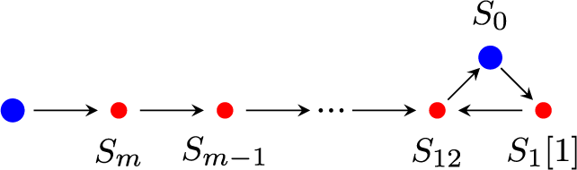
Figure 3 Mutation at $S_1$ of the ext-quiver of Figure 2.

Tilting inductively at $S_{1\dots i}$ (recall the notation from (3)), the procedure leads to a configuration where such a sequence has length $0$ , as desired, see Figure 4. We define $\mathcal X = \langle S_{1\dots m},\ldots , S_1\rangle $ so that $\mu ^\sharp _{\mathcal {X}}:=\mu ^\sharp _{S_{1\dots m}}\cdots \mu ^\sharp _{S_1}$ by Proposition 2.2. By construction, $\mathcal {X} \subset {\mathcal A}\cap {\mathcal V}$ and $\overline {\mu ^\sharp _{\mathcal {X}}{\mathcal A}}= \overline {{\mathcal A}}\subset {\mathcal D}/{\mathcal V}$ .

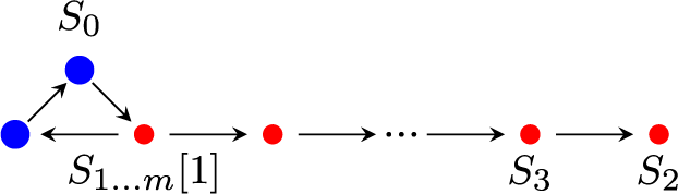
Figure 4 The result of mutating at $S_1, S_{12},\dots , S_{1\dots m}$ the ext-quiver of Figure 2.

Suppose now that there exists another simple $S_1^{\prime }\neq S_1$ satisfying (23). Proceeding in the same way, we define $S_i^{\prime }$ using (23) and (24) and define inductively $S^{\prime }_{1\dots i}$ for $i=1,\dots ,m'$ as above. They are not in $\langle S_1,\dots , S_{m+1}\rangle $ , due to the second condition in (24). Then, with $\mathcal X' = \langle S^{\prime }_{1\dots m},\ldots , S^{\prime }_1\rangle $ ,

$$ \begin{align*}\mu^\sharp_{\mathcal{X}'}\mu^\sharp_{\mathcal{X}}\left({\mathcal A}\right)=(\mu^\sharp_{S^{\prime}_{1\dots m'}}\cdots\mu^\sharp_{S^{\prime}_{12}}\mu^\sharp_{S^{\prime}_1})(\mu^\sharp_{S_{1\dots m}}\cdots \mu^\sharp_{S_{12}}\mu^\sharp_{S_1})({\mathcal A})\end{align*} $$

is a convenient representative of $\overline {{\mathcal A}}$ with respect to $S_0$ .

For later use, we record that the ‘lifts’ of the tilts at ${\overline {\mathcal {F}}_{i}}$ used in the previous proof are actually tilts at explicit torsion-free classes $\mathcal F_i$ .

Lemma 4.10. Recall that ${\mathcal D} = {\mathcal D}_{A_n}$ , and let ${\mathcal A}_\bullet =({\mathcal A}_0,{\mathcal A}_1)$ and $Z_\bullet = (Z_0,Z_1)$ . For $\lambda \in \mathbb {R}_{\geq 0}$ such that

• ○ $\lambda \cdot (\overline {{\mathcal A}_0},\overline {Z_0})=(\mu ^\sharp _{S_0}\overline {{\mathcal A}_0}, e^{-\pi \lambda }\overline {Z_0})$ in $\operatorname {Stab}^\circ ({\mathcal D}/{\mathcal V})$ , and

• ○ there are no indecomposables in ${\mathcal A}_1$ with phase $\phi _{\overline {Z_1}}$ less than or equal to $\lambda $ ,

the action by $\lambda $ on $[{\mathcal A}_\bullet ,Z_\bullet ]$ gives $[{\mathcal A}^{\prime }_\bullet ,Z^{\prime }_\bullet ]$ with nested hearts

$$\begin{align*}{\mathcal A}^{\prime}_0 \;=\;\mu^\sharp_{\mathcal{F}}{\mathcal A}_0, \quad {\mathcal A}^{\prime}_1 \;=\;{\mathcal A}_1, \end{align*}$$

for $\mathcal {F}=\langle S^{\prime }_{01\dots m'}, \dots S^{\prime }_{01},S_{01\dots m}, \dots S_{01}, S_0\rangle $ , using the same notation as in proof of Lemma 4.9. Moreover, $\mathcal {F}\subset \langle S_0,{\mathcal A}_1\rangle \setminus {\mathcal A}_1$ .

Proof. Suppose for simplicity $m>0$ , $m'=0$ in the notation of Lemma 4.9. We know that ${\mathcal A}^{\prime }_0=\mu ^\flat _{\mathcal X[1]} \mu ^\sharp _{S_0}\mu ^\sharp _{\mathcal X}{\mathcal A}_0$ by the procedure described in the proof of Proposition 4.6. Since

$$\begin{align*}\langle S_0,S_{01}, \dots, S_{01\dots m}, S_1,\dots, S_{1\dots m}\rangle \;=\; \langle S_1, S_{12},\dots, S_{1\dots m}, S_0\rangle,\end{align*}$$

we deduce that

$$\begin{align*}(\mu^\sharp_{S_{1\dots m}}\cdots\mu^\sharp_{S_{1}}) (\mu^\sharp_{S_{01\dots m}}\cdots \mu^\sharp_{S_{01}}) \mu^\sharp_{S_0}({\mathcal A}) \;=\; \mu^\sharp_{S_0} (\mu^\sharp_{S_{1\dots m}} \cdots \mu^\sharp_{S_1})({\mathcal A}),\end{align*}$$

and hence, $\mu ^\sharp _{\mathcal {F}} ({\mathcal A})= \mu ^\flat _{\mathcal X[1]} \mu ^\sharp _{S_0} \mu ^\sharp _{\mathcal X}({\mathcal A}).$

We use the subsequent lemma as a preparation for Proposition 5.2 below.

5.1 Plumbing of stability conditions

The plumbing construction takes as input a multi-scale stability condition $(\mathcal {A}_\bullet , Z_\bullet )$ and a collection ${\boldsymbol {\tau }}=(\tau _1,\ldots ,\tau _L) \in -\mathbb {H}^L$ and outputs an honest stability condition. More generally, we will allow ${\boldsymbol {\tau }}$ to take the formal value $\tau _j = -i\infty $ for j in any fixed subset $J \subset \{1,\ldots L\}$ and let $-\mathbb {H}_\infty = -\mathbb {H} \cup \{-i\infty \}$ . The result of the plumbing construction will then be a multi-scale stability condition with $|J|$ levels below zero, the extreme case ${\boldsymbol {\tau }} = (-i\infty )^L$ being the identity, no plumbing at all. Using all tuples ${\boldsymbol {\tau }}$ with each entry of large (or infinite) imaginary part and then allowing small deformations of the resulting generalized stability conditions at each level will provide a neighborhood of $(\mathcal {A}_\bullet ,Z_\bullet )$ .

For simplicity, we start with a multi-scale stability conditions $(\mathcal {A}_\bullet ,Z_\bullet )$ with $L=1$ and let ${\mathcal V} = {\mathcal V}_1^Z$ .

Note that the plumbing procedure depends on a chosen representative. For the definition of the topology, we will use that the set $\{ \tau \ast (\mathcal {A}_\bullet ,Z_\bullet ), \, -\Im (\tau )> C\}$ for any fixed C does not depend on this representative, since the change of representative results in translation of the corresponding $\tau $ by a real number. We use that

(25) $$ \begin{align} K({\mathcal A}_0) = K(\overline{{\mathcal A}_0}) \oplus K({\mathcal A}_1) \quad \text{given by} \quad \operatorname{Sim}({\mathcal A}_0) = \operatorname{Sim}(\overline{{\mathcal A}_0}) \,\coprod\, \operatorname{Sim}({\mathcal A}_1) \end{align} $$

(see, for example, the survey [Reference PsaroudakisPsa18, Proposition 2.9]) to define two projections

(26) $$ \begin{align} \pi_0:K({\mathcal D})\simeq K({\mathcal A}_0)\to K(\overline{{\mathcal A}_0}), \quad \pi_1: K({\mathcal D})\simeq K({\mathcal A}_0)\to K({\mathcal A}_1)\,. \end{align} $$

Using these projections, we combine central charges as

$$ \begin{align*} Z_0 \oplus Z_1 \,:= \,Z_0 \circ \pi_0 + Z_1 \circ \pi_1\,. \end{align*} $$

Next, we generalize to the action of ${\boldsymbol {\tau }} = (\tau , -i\infty , \ldots , -i\infty )$ on a multi-scale stability condition $(\mathcal {A}_\bullet ,Z_\bullet )$ . In this case, we apply Proposition 5.1 to the first two levels $( ({\mathcal A}_0, {\mathcal A}_1),(Z_0,Z_1))$ and record as ${\boldsymbol {\tau }}$ -image the tuple

(27) $$ \begin{align} (\tau, -i\infty, \ldots, -i\infty) \cdot (\mathcal{A}_\bullet,Z_\bullet) \;=\; ({\mathcal A}', {\mathcal A}_2,{\mathcal A}_3 \ldots,Z',Z_2,Z_3,\ldots)\, \end{align} $$

(i.e., the top two levels have been merged to obtain a multi-scale stability condition with $L-1$ levels below zero).

This construction also gives a recipe for the plumbing ${\boldsymbol {\tau }} \ast (\mathcal {A}_\bullet ,Z_\bullet )$ of a multi-scale stability condition $(\mathcal {A}_\bullet ,Z_\bullet )$ by a general ${\boldsymbol {\tau }} \in -\mathbb {H}_\infty ^L$ . We take j to be the highest index with $\tau _j \neq -i\infty $ . Then we apply the preceding construction to the multi-scale stability condition $( {\mathcal A}_{\geq j},Z_{\geq j})$ on ${\mathcal V}_j^Z$ and iterate with the action of the remaining coordinates ${\boldsymbol {\tau }}' = (\tau _1, \cdots , \widehat {\tau _j}, \cdots )$ . It will turn out that the plumbing procedure is not quite independent of the order of the levels at which we perform the plumbing step, only nearly so. The reason is that already one-level plumbing and rotation are only nearly compatible. We need a quantitative version of this fact.

Proposition 5.2. Let $(\mathcal {A}_\bullet ,Z_\bullet )$ be a fixed representative of a multi-scale stability condition with $L=1$ . Let $\tau \in -{\mathbb H}$ , $\lambda \in \mathbb {C}$ , with

(28) $$ \begin{align} 0\leq \Re\lambda,\quad 0 \leq \Re\tau, \quad \text{and}\quad 0\leq \Re (\lambda+\tau)<1. \end{align} $$

Then the hearts of the two stability conditions

(29) $$ \begin{align} \widetilde{\sigma}:=(\widetilde{{\mathcal A}},\widetilde{Z}):=\lambda \cdot (\tau \ast (\mathcal{A}_\bullet,Z_\bullet)) \quad \text{and} \quad \widehat{\sigma}:=(\widehat{{\mathcal A}},\widehat{Z}) :=\tau \ast (\lambda \cdot (\mathcal{A}_\bullet,Z_\bullet)) \end{align} $$

are intermediate hearts with respect to ${\mathcal A}_0$ , and the difference of the central charges may be coarsely estimated by

(30) $$ \begin{align} \left|(\widehat{Z}-\widetilde{Z})(S_j)\right| \,\leq \, \ell \cdot |e^{-\pi i (\lambda+\tau)}| \sum_{\substack{S_i\in{\mathcal A}_1\\\text{simple}}} |Z_1(S_i)| \end{align} $$

for any simple $S_j \in \operatorname {Sim}({\mathcal A}_0)$ , where $\ell $ is the number of classes of indecomposables in $K(\overline {{\mathcal A}_0})$ .

We recall from [Reference BridgelandBri16, Proposition 7.4] that the local homeomorphism given by the forgetful map is actually injective when restricted to all hearts that are intermediate with respect to a given heart ${\mathcal A}_0$ (i.e., in $[{\mathcal A}_0,{\mathcal A}_0[1]]$ ). Consequently, to show that $\widetilde {\sigma }$ and $\widehat {\sigma }$ are nearby, it suffices to estimate the differences of the central charges if $\widetilde {{\mathcal A}}, \widehat {{\mathcal A}} \in [{\mathcal A}_0,{\mathcal A}_0[1]]$ .

Proof. The result of plumbing is given by definition as $({\mathcal A}, Z):=\tau \ast (\mathcal {A}_\bullet ,Z_\bullet )$ with

$$\begin{align*}\begin{aligned} &{\mathcal A}=\mu_{\mathcal{F}_\tau}^\sharp{\mathcal A}_0\supset\mu_{\mathcal{F}_\tau}^\sharp{\mathcal A}_1,\quad \mathcal{F}_\tau=\langle E\in {\mathcal A}_1,\, Z_1\text{-semistable s.t. }\phi_{Z_1}(E)\leq \Re\tau\rangle\\ &Z := \overline{Z_0} \oplus e^{-i\pi\tau} \cdot Z_1\,. \end{aligned}\end{align*}$$

We first consider the case where

• ( $\star $ ) there is exactly one isomorphism class $[S_0]\in K({\mathcal A})$ of a Z-stable object in ${\mathcal A}$ with phase ${0<\phi _Z(S_0)\leq \Re \lambda }$ , and moreover, $[S_0] \not \in K({\mathcal V})$ .

(Note that $S_0$ must be simple in ${\mathcal A}$ .) In this case, the stability condition $\widetilde {\sigma }$ is given by $\widetilde {Z} =e^{-i\pi \lambda }Z$ and $\widetilde {{\mathcal A}} =\mu ^\sharp _{S_0}{\mathcal A} = \mu ^\sharp _{\widetilde {\mathcal F}}{\mathcal A}_0$ with $\widetilde {\mathcal F} = \langle \mathcal F_\tau , S_0 \rangle $ . In particular, $\widetilde {{\mathcal A}} \in [{\mathcal A}_0,{\mathcal A}_0[1]]$ .

However, the heart $\widehat {{\mathcal A}}$ is obtained by $\tau $ -plumbing the multi-scale heart $({\mathcal A}_1 \subset \mu ^\sharp _{\mathcal {F}}{\mathcal A}_0)$ , where ${\mathcal {F}=\langle S_0,S_{01},\dots \rangle \subset {\mathcal A}_0}$ is explicitly described in Lemma 4.10, since assumption $(\star )$ implies that the torsion-free class in $\overline {{\mathcal A}_0}$ of objects with phase $0<\phi _{\overline {Z_0}}\leq \Re \lambda $ is generated by $\overline {S_0}$ . Consequently,

$$ \begin{align*} \widehat{{\mathcal A}}\;=\;\mu^\sharp_{\mathcal{G}} \mu^\sharp_{\mathcal{F}}{\mathcal A}_0, \quad \text{where} \quad \mathcal{G} \;=\; \langle E\in {\mathcal A}_1,\, Z_1\text{-semistable s.t. }\phi_{Z_1}(E)\leq \Re\tau\rangle. \end{align*} $$

Since $\mathcal {G} \subset \mu ^\sharp _{\mathcal {F}}{\mathcal A}_0\cap {\mathcal V}_1$ and $\mu ^\sharp _{\mathcal {F}}{\mathcal A}_1 = {\mathcal A}_1$ , we deduce $\mathcal {G} \cap \mathcal {F}[1] =\{0\}$ , and consequently (by the same arguments as in Lemma 4.11), we deduce ${\mathcal A}_0\leq \mu ^\sharp _{\mathcal {F}}{\mathcal A}\leq \widehat {{\mathcal A}} = \mu ^\sharp _{\mathcal {G}} \mu ^\sharp _{\mathcal {F}}{\mathcal A}_0 \leq {\mathcal A}_0[1]$ in the partial order from Section 2.1.

To compare central charges, note that the plumbing procedure happens over two different decompositions of $K({\mathcal D})$ : one induced by $K({\mathcal A}_0/{\mathcal A}_1) \oplus K({\mathcal A}_1)$ , and the other induced by $K(\mu _{\mathcal {F}}^\sharp {\mathcal A}_0/{\mathcal A}_1) \oplus K({\mathcal A}_1)$ . The change of basis $K(\mu ^\sharp _{\mathcal {F}}{\mathcal A}_0) \simeq K({\mathcal A}_0)=K({\mathcal A}_0/{\mathcal A}_1)\oplus K({\mathcal A}_1)$ has the form of a block lower-triangular matrix

$$\begin{align*}\left[\mu_{\mathcal{F}}\right]^{-1}=\begin{pmatrix} C_{n-k} & 0 \\ B_{1\overline{0}} & \mathbf{1}_k\end{pmatrix}, \end{align*}$$

where the entries of $B_{1\overline {0}}=(b_{ij})_{ij}$ have absolute value at most $1$ , where we hardly control the block $C_{n-k}$ , and where the block $\mathbf {1}_k$ expresses that ${\mathcal V}$ is preserved. Using the projections $\pi _0$ and $\pi _1$ onto the summands $K({\mathcal A}_0/{\mathcal A}_1)\oplus K({\mathcal A}_1)$ , we find

$$\begin{align*}\widetilde{Z} \;=\;e^{-\pi i \lambda}\overline{Z_0}\circ\pi_0 + e^{-\pi i (\lambda+\tau)} Z_1\circ\pi_1 \end{align*}$$

and

(31) $$ \begin{align}\begin{aligned} \widehat{Z}&\;=\; e^{-\pi i \lambda}Z_0\circ\widehat{\pi}_0 + e^{-\pi i (\tau+\lambda)}Z_1\circ\widehat{\pi}_1\\ &\ =e^{-\pi i \lambda}Z_0\circ\pi_0 + e^{-\pi i (\tau+\lambda)}Z_1\circ(\pi_1+B_{1\overline{0}}\pi_0), \end{aligned}\end{align} $$

where we see $B_{1\overline {0}}$ as a map $K({\mathcal A}_0/{\mathcal A}_1)\to K({\mathcal A}_1)$ . Now consider the simples in ${\mathcal A}_0$ . For $S_j\in {\mathcal A}_1$ , the two expressions agree. For $S_j$ a simple of ${\mathcal A}_0$ not in ${\mathcal A}_1$ , we find

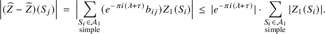$$ \begin{align*} \left|(\widehat{Z}-\widetilde{Z})(S_j)\right| \;=\; \Bigl|\sum_{\substack{S_i\in{\mathcal A}_1\\\text{simple}}}(e^{-\pi i (\lambda+\tau)}b_{ij})Z_1(S_i)\Bigr| \,\leq\, |e^{-\pi i (\lambda+\tau)}| \cdot \sum_{\substack{S_i\in{\mathcal A}_1\\\text{simple}}} |Z_1(S_i)|. \end{align*} $$

We now drop the assumption ( $\star $ ) and allow for multiple indecomposables $X\in {\mathcal A}$ with $0<\phi _Z(X)\leq \Re \lambda $ .

The assumption (28) still guarantees that $\widetilde {{\mathcal A}}\in \left [{\mathcal A}_0,{\mathcal A}_0[1]\right ]$ , and $\widetilde {Z}=e^{-\pi i \lambda }\overline {Z_0}\circ \pi _0 + e^{-\pi i (\lambda +\tau )}Z_1 \circ \pi _1$ , as before.

The result of $\lambda \cdot ({\mathcal A}_\bullet , Z_\bullet )$ is a multi-scale stability condition $\sigma '$ with nested hearts ${\mathcal A}_1^{\prime } \subset {\mathcal A}_0^{\prime }$ that can be explicitly obtained as in the proof of Proposition 4.6 by performing a forward-tilt at $\mathcal {F}_\lambda ^1$ and a sequence of forward-tilts at torsion-free classes $\mathcal {F}_i$ described in Lemma 4.10 and Lemma 4.11. At each step, at the 0 level, the matrix of the change of basis has the form of a block lower triangular matrix, with a block $B_{1\bar {0}}= \prod _i B_{1\bar {0}}^{(i)}$ , whose entries have absolute value $\leq \ell ^{\prime }_i$ , bounded by the number $\ell ^{\prime }_i$ of classes of indecomposables in $\mathcal {F}^1_\lambda $ or $\mathcal {F}_i$ . Lemma 4.11 guarantees that the heart ${\mathcal A}_0^{\prime }$ is intermediate with respect to ${\mathcal A}_0$ , and so is the heart of $\tau *\sigma '$ thanks to assumption 28. Similarly to (5.1), we obtain

$$\begin{align*}\left|(\widehat{Z}-\widetilde{Z})(S_j)\right| \leq |e^{-\pi i (\lambda+\tau)}| \cdot \ell\sum_{\substack{S_i\in{\mathcal A}_1\\\text{simple}}} |Z_1(S_i)|, \end{align*}$$

where $\ell $ is the number of classes of indecomposables in $K({\mathcal A}_0)$ . Last, the case $\Re \lambda =0$ is just easier, and the argument above shows that in such a case, $\lambda \cdot (\tau \ast ({\mathcal A}_\bullet ,Z_\bullet )) =\tau \ast (\lambda \cdot ({\mathcal A}_\bullet ,Z_\bullet ))$ .

Remark 5.3. The same observation shows that the plumbing (with fixed parameter $\tau \in -\mathbb {H}$ ) of a path is not continuous. Discontinuities occur when some simple (not at bottom level) is tilted. However, the size of the jumps decreases with $|e^{-\pi i \tau }|$ . More precisely, suppose that $L=1$ and that $\gamma $ is a path for which at precisely one value $t_0 \in [0,1]$ , such a tilt occurs. Then the hearts of the two stability conditions

$$ \begin{align*} {\sigma}^+:=({{\mathcal A}}^+,{Z}^+):=\lim_{t \to t_0^+} (\tau \ast \gamma(t)) \quad \text{and} \quad {\sigma}^-:=({{\mathcal A}}^-,{Z}^-):=\lim_{t \to t_0^-} (\tau \ast \gamma(t)) \end{align*} $$

are intermediate hearts with respect to the top level heart ${\mathcal A}_0$ of $\lim _{t \to t_0^-}\gamma (t_0)$ , and the difference of the central charges may be coarsely estimated by

(32) $$ \begin{align} \left|({Z}^+-{Z}^-)(S_j)\right| \,\leq \, \ell \cdot |e^{-\pi i \tau}| \sum_{\substack{S_i\in{\mathcal A}_1\\\text{simple}}} |Z_1(S_i)| \end{align} $$

for any simple $S_j \in \operatorname {Sim}({\mathcal A}_0)$ , where $\ell $ is the number of classes of indecomposables in $K(\overline {{\mathcal A}_0})$ . The proof is exactly the same as for the previous proposition.

Let again $0 \leq \Re (\tau ) < 1$ , and decompose $\tau = \tau _R + i \tau _I$ into its real and imaginary part. We observe that the plumbing in Proposition 4.6 can be viewed a composition of three steps: First, we apply the action of $\tau _R$ , resulting in a tilt at a torsion-free class $\mathcal F \subset {\mathcal A}_1$ and turning $Z_1$ by $e^{-\pi i \tau _R}$ resulting in some other representative $({\mathcal A}_\bullet ^{\Re (\tau )}, Z_\bullet ^{\Re (\tau )})$ of the multi-scale stability condition. Second, we rescale $e^{-\pi i \tau _R}Z_1$ by $e^{\pi \tau _I}$ , and finally, we form the direct sum Z and drop the lower levels to get an honest stability condition. The observation that $[\mu ^\sharp _{\mathcal {F}}]^{-1}$ in the previous proof preserves ${\mathcal V}_1$ and the first step just described does preserve ${\mathcal V}_1$ as well, together imply the following corollary where we relax the bound for $\Re (\tau )$ appearing in Proposition 5.2.

Corollary 5.4. Let $(\mathcal {A}_\bullet ,Z_\bullet )$ be a fixed representative of a multi-scale stability condition with $L=1$ . Let $\tau \in -{\mathbb H}$ , $\lambda \in \mathbb {C}$ , with $0 \leq \Re (\lambda ) < 1$ . Then the hearts of the two stability conditions

$$ \begin{align*} \widetilde{\sigma}:=(\widetilde{{\mathcal A}},\widetilde{Z}):=\lambda \cdot (\tau \ast (\mathcal{A}_\bullet,Z_\bullet)) \quad \text{and} \quad \widehat{\sigma}:=(\widehat{{\mathcal A}},\widehat{Z}) :=\tau \ast (\lambda \cdot (\mathcal{A}_\bullet,Z_\bullet)) \end{align*} $$

are intermediate hearts with respect to ${\mathcal A}_0^{\Re (\tau )}$ , and the difference of the central charges may be coarsely estimated as in (30).

5.2 Neighborhoods in the space $\operatorname {MStab}^\circ ({\mathcal D}^3_{A_n})$

We work here with a representative $(\mathcal {A}_\bullet ,Z_\bullet )$ of a multi-scale stability condition and let

$$ \begin{align*}{\boldsymbol{\delta}} = (\delta_1,\ldots,\delta_L)\end{align*} $$

be a tuple of (small) positive real numbers where $\delta _j$ will control the size of plumbing of level j. Moreover, we fix a collection of positive real numbers

$$ \begin{align*}{\boldsymbol{\varepsilon}} \;=\; (\varepsilon_J) \quad \text{for any} \quad J\subset \{0,\ldots,L\}.\end{align*} $$

The following Definition 5.6 captures the idea that neighborhoods of boundary points consist of the multi-scale stability conditions, described heuristically as follows. Suppose $L=1$ for simplicity. We write $\epsilon _0,\epsilon _1,\epsilon _{01}$ for $J=\{0\},\{1\},\{0,1\}$ , respectively. Then

• ○ we may plumb by $\tau $ with large negative imaginary part (so that the lower level stability condition $({\mathcal A}_1,e^{-\pi i \tau } Z_1)$ stays small in size) and wiggle the result in by a small amount (by a size controlled by $\varepsilon _{01}$ );

• ○ alternatively, we may not plumb (i.e., $\tau = -i\infty $ ) and wiggle in and a bit (by sizes controlled by $\varepsilon _i$ ) on level i, for $i=0,1$ .

We say that a stability condition $(\mathcal {A}_\bullet ^{\prime },Z^{\prime }_\bullet )$ with $L' \leq L$ levels below zero arises by plumbing of size at most ${\boldsymbol {\delta }}$ from $(\mathcal {A}_\bullet , Z_\bullet )$ if there is $\tau \in (-\mathbb {H}_\infty )^L$ ) with $|e^{-\pi i \tau _j}| < \delta _j $ for $j=1,\ldots ,L$ and $({\mathcal A}^{\prime }_\bullet ,Z^{\prime }_\bullet ) = \tau \ast ({\mathcal A}_\bullet ,Z_\bullet )$ . For a such a stability condition, we denote the new vanishing categories by ${\mathcal V}^{\prime }_i$ . Say levels in the interval $J_i = \{j_1,\ldots \} \subset \{0,\ldots ,L\}$ have been plumbed to form the new level i. (This implies by definition that $\tau _{j_1} = -i\infty $ .)

We define the natural inner product on by using as an orthonormal basis the basis $Z_{S_i}$ dual to the simples of ${\mathcal A}_0$ . (Note that this norm depends on the heart ${\mathcal A}_0$ and its simples, but the norm around any other multi-scale stability condition $\sigma ^\dagger = (\mathcal {A}_\bullet ^\dagger ,Z^\dagger _\bullet )$ is comparable, scaling by a factor $C = C(\sigma ,\sigma ^\dagger )$ given by the operator norm of the identity map with respect to the to norms.)

This definition includes the case that $L=0$ and that $(\mathcal {A}, Z)$ is an honest stability condition, in which case, the neighborhoods have to contain the $\varepsilon $ -balls in the norm with orthonormal bases given by the simples of $\mathcal {A}$ , since the deformation of stability conditions is locally controlled by the deformation of the central charge. This gives the second part of the following lemma.

Proof. The only axiom whose verification is nontrivial is the following. Let U be a neighborhood of $\sigma =[A_\bullet ,Z_\bullet ]$ , in the sense of Definition 5.6. Then there is a smaller neighborhood V of this point, such that U is a neighborhood of each $\sigma ^\dagger =[{\mathcal A}^\dagger _\bullet ,Z^\dagger _\bullet ]$ in V. We continue with the case $L = 1$ ; the general case works with the same argument. By definition, U contains some $V_{{\boldsymbol {\varepsilon }},\delta }(A_\bullet ,Z_\bullet )$ . The rough idea is to take $V = V_{{\boldsymbol {\varepsilon }}^*,\delta ^*}(A_\bullet ,Z_\bullet )$ for some $({\boldsymbol {\varepsilon }}^*,\delta ^*)$ smaller than $({\boldsymbol {\varepsilon }}, \delta )$ in each entry, so that U contains $V_{({\boldsymbol {\varepsilon }}-{\boldsymbol {\varepsilon }}^*)/C, \delta -\delta ^*}(\sigma ^\dagger )$ , just as if we would be working plainly in vector spaces, where $C = C(\sigma ,\sigma ^\dagger )\geq 1$ accounts for the change of basis in the definition of the norms. We will prove that $V_{({\boldsymbol {\varepsilon }}-{\boldsymbol {\varepsilon }}^*)/C, \delta -\delta ^*}(\sigma ^\dagger )$ is indeed contained in $V_{{\boldsymbol {\varepsilon }},\delta }(\sigma )$ for ${\boldsymbol {\varepsilon }}^*$ carefully chosen. We have to avoid that $\varepsilon _0^*$ , $\varepsilon _1^*$ are large compared to $\varepsilon _{01}^*$ so that any plumbing after deforming $({\mathcal A}^\dagger _\bullet ,Z^\dagger _\bullet )$ of the order of $\varepsilon _0$ , $\varepsilon _1$ does not fail of being near $\sigma $ .

We may thus first take the pair $(\varepsilon _0^*, \varepsilon _1^*)$ so small that any point in the $(\varepsilon _0^*, \varepsilon _1^*)$ -ball in can be reached from $\sigma $ by a path $\gamma (t)$ involving at most one tilt, at $t=0$ . Suppose the chosen $\sigma ^\dagger =(A_\bullet ^\dagger , Z_\bullet ^\dagger )\in V_{{\boldsymbol {\varepsilon }}^*,\delta ^*}(\sigma )$ has also $L = 1$ levels below zero, and let $\gamma ^\dagger (t)$ be the straight path connecting $\sigma $ and $\sigma ^\dagger $ . Let $\tau $ in $-{\mathbb {H}}$ of magnitude at most $\delta ^*$ , and $\hat \sigma =\tau *\sigma ^\dagger $ , $\sigma '=\tau *\sigma $ . By the argument in Proposition 5.2 and the one-tilt hypothesis, the hearts $\hat {\mathcal {A}}$ and ${\mathcal A}'$ are intermediate with respect to ${\mathcal A}_0$ , so the distance between $\hat \sigma $ and $\sigma '$ is controlled by their central charges. If the plumbing of the path $\gamma ^\dagger $ is continuous, then

(33) $$ \begin{align} ||\widehat{Z} - Z'|| \leq \varepsilon_0^* + \delta_1^*\varepsilon_1^*\,. \end{align} $$

In the general case of a single tilt, use Remark 5.3 and compare $\sigma ' = \sigma ^-$ with $\sigma ^+ := ({\mathcal A}^+,Z^+) = \lim _{t \to 0^+} \tau *\gamma ^\dagger (t)$ . Now (32) and the previous estimate in the new notation give the rough estimate

(34) $$ \begin{align} ||\widehat{Z} - Z^+|| \leq \varepsilon_0^* + \delta_1^*\varepsilon_1^*\,\quad \text{and} \quad\,||Z^+ - Z'|| \leq \ell n \delta_1^*. \end{align} $$

The triangle inequality shows that requiring, moreover, $\varepsilon _{01}^* \leq \varepsilon _0^* + \delta _1^*(\varepsilon _1^* + \ell n)$ does the job.

The next lemma will be used in the proofs at the end of this section. We consider a sequence $\{\sigma _j\}_j$ of multi-scale stability conditions in $\operatorname {MStab}^\circ ({\mathcal D}_{A_n}^3)$ .

5.3 The complex structure on quotients of boundary neighborhoods in $\operatorname {MStab}^\circ ({\mathcal D}^3_{A_n})$

Next, we upgrade from a topology to a structure of complex orbifold. This will not be possible on $\operatorname {MStab}^\circ ({\mathcal D}^3_{A_n})$ , but only the quotient by the group of autoequivalences; see Section 6.4 for an illustration in the case of the $A_2$ -quiver. The first step in this direction is to exhibit a subgroup ${\operatorname {Tw}}^s({\mathcal V}_\bullet )$ in the stabilizer of the boundary such that the quotient $\operatorname {MStab}^\circ ({\mathcal D},{\mathcal V}_\bullet )/{\operatorname {Tw}}^s({\mathcal V}_\bullet )$ is a complex manifold. We then determine the full stabilizer of these boundary neighborhoods and exhibit the orbifold structure.

We fix once for all a multi-scale stability condition $\sigma _\bullet =[{\mathcal A}_\bullet ,Z_\bullet ]$ with L levels below zero, and let ${\mathcal V}_\bullet $ be the associated sequence of nested vanishing subcategories of ${\mathcal D}={\mathcal D}^3_{A_n}$ .

The simple twist group $\mathit {Tw}^{s}({\mathcal V}_{\bullet})$

Recall the numerical data associated with a multi-scaled stability conditions of type $A_n$ from Section 4.1, and suppose $\sigma _\bullet $ is of type ${\boldsymbol {\rho }}$ . We focus at a level i, and let ${\mathcal V}_i^{(j)}$ be the components of ${\mathcal V}_i$ . Suppose that ${\mathcal V}_i^{(j)}$ has type $n_{i}^{(j)}$ (i.e., the heart ${\mathcal V}_i^{(j)}\cap {\mathcal A}_i$ has $n_{i}^{(j)}$ simples $S_1,\ldots ,S_{n_{i}^{(j)}}$ in the subset $\mathcal S = \mathcal S(i,j)$ of $\operatorname {Sim}({\mathcal A}_0)$ ). We recall the definition in Section 3.3 of the group elements $\theta _{I,n}$ .

For I denoting the closed arcs in the subsurface $\Sigma _i^{(j)}$ , we let

(35) $$ \begin{align} \mathfrak{c}_{i,j} = \begin{cases} \theta_{I,n} & \text{if } n_i^{(j)} \text{ is odd}\\ \theta_{I,n}^2 & \text{if } n_i^{(j)} \text{ is even.} \end{cases} \end{align} $$

From ${\boldsymbol {\rho }}$ , we derive another collection of integers $(\ell _i)_{i=1}^L$ . Recall that we define $\kappa _i^{(j)} = n_i^{(j)} + 3$ to be the number of marked points on the boundary of $\Sigma _i^{(j)}$ . We let

(36) $$ \begin{align} \widehat{\kappa}_i^{(j)} \;=\; \begin{cases} (n_i^{(j)} + 3)/2 & \text{if } n_i^{(j)} \text{ is odd} \\ (n_i^{(j)} + 3) & \text{if } n_i^{(j)} \text{ is even.} \\ \end{cases} \end{align} $$

(This notation is consistent with the enhancements in Section 6.) We define

(37) $$ \begin{align} \ell_i \;=\; \operatorname{lcm}\{ \widehat{\kappa}_i^{(j)}\,,\, j=1,\ldots, s_i \}\,. \end{align} $$

For each level i and each j, we now define the elements

(38) $$ \begin{align} \mathfrak{c}_i := \prod_j \mathfrak{c}_{i,j}^{\ell_i/\widehat{\kappa}_{i}^{(j)}} := \prod_j \theta_{I(i,j),n}^{\ell_i/\kappa_i^{(j)}}. \end{align} $$

and we define the simple twist group to be ${\operatorname {Tw}}^s({\mathcal V}_\bullet ) :=\langle \mathfrak {c}_1,\dots , \mathfrak {c}_L\rangle $ .

Proposition 5.11. For each level i, the element preserves the neighborhoods $V_{{\boldsymbol {\varepsilon }},\delta }({\mathcal A}_\bullet ,Z_\bullet )$ for all $({\boldsymbol {\varepsilon }},\delta )$ small enough.

Implicit in the notation is that the elements $\mathfrak {c}_{i,j}$ for fixed j commute. In fact, we have the following:

Lemma 5.12. The elements $\mathfrak {c}_{i,j}$ for all $(i,j)$ commute. In particular, the simple twist group ${\operatorname {Tw}}^s({\mathcal V}_\bullet ) = \langle \mathfrak {c}_1,\dots , \mathfrak {c}_L\rangle $ is a free abelian group of rank L.

Proof. For fixed i, the elements $\mathfrak {c}_{i,j}$ and $\mathfrak {c}_{i,j'}$ commute by (14) since they correspond to disjoint subsurfaces, and hence, any two vertices, one in $I(i,j)$ and one in $I(i,j')$ , cannot be connected by an edge in the corresponding quiver. For different level indices $i < i'$ , the elements $\mathfrak {c}_{i,j}$ and $\mathfrak {c}_{i',j'}$ commute for the same reason if $Q_{I(i',j')}$ is not a subquiver of $Q_{I(i,j)}$ . If it is a subquiver, the elements commute since $\theta _{I,n}$ is (the image of) the central element in the braid group corresponding to $Q_{I(i,j)}$ .

Proof of Proposition 5.11

Focusing on the subcategories above and below i, we may reduce to the case that $({\mathcal A}_\bullet ,Z_\bullet )$ has $L=1$ and we consider $i=1$ , thus writing ${\mathcal V} = {\mathcal V}_1$ . Suppose the connected components ${\mathcal V}^{(j)}$ have type $n_j$ and correspond to the subsurfaces $\Sigma ^{(j)}$ . We claim that

(39)

Granting the claim, we conclude that $\mathfrak {c}_{1}$ acts like the shift by $\ell _1$ on ${\mathcal A}_1 \cap {\mathcal V}^{(j)}$ for every j, and thus on the whole $({\mathcal A}_1,Z_1)$ . Since adding $\widehat {\kappa }_{1}^{(j)}$ to $\tau $ does not change the norm used in (1) of the topology definition, the elements stabilize the neighborhoods, as claimed. Since $\tau +\widehat {\kappa }_{1}^{(j)}$ realizes a plumbing of size at most $\delta $ , if $\tau $ does so, the elements stabilize the neighborhoods (as defined by (1)–(2) in Definition 5.6), as claimed.

The first equality of (39) is [Reference Seidel and ThomasST01, Lemma 4.14] applied to the subquiver $Q_{I(1,j)}$ . The second equality holds by definition of the induced actions on Grothendieck groups; see (19). For the third equality, we write each spherical twist appearing in the definition of $\mathfrak {c}_{1,j}$ as a composition of tilts at simples in ${\mathcal V}$ using (16). The claim then follows since such tilts do not change the quotient heart; see [Reference Barbieri, Möller, Qiu and SoBMQS22, Lemma 5.6].

The complex structure on boundary neighborhoods

Consider a neighborhood $V_{{\boldsymbol {\varepsilon }},\delta }({\mathcal A}_\bullet ,Z_\bullet )$ as given in Definition 5.6. As we stated after (39), the element $\mathfrak {c}_i$ acts as the shift by $\ell _i$ on the i-th level of $({\mathcal A}_\bullet ,Z_\bullet )$ . Consequently, plumbing by ${\boldsymbol {\tau }}$ and plumbing by ${\boldsymbol {\tau }} + \ell _i e_i$ (where $e_i$ is the i-th unit vector) give the same stability condition in the quotient $V_{{\boldsymbol {\varepsilon }},\delta }( {\mathcal A}_\bullet ,Z_\bullet )/ {\operatorname {Tw}}^s({\mathcal V}_\bullet )$ . Therefore, on this quotient space, the parameters

• ○ $t_i = \exp \{2 \pi \sqrt {-1} \frac {\tau _i}{\ell _i}\}$ for $i=1,\ldots , L$ ,

• ○ the ratios of central charges of simples on for $j>0$ ,

• ○ the central charges of the simples on

all together give a complex chart.

Instead of using ratios of central charges, we may equivalently fix a representative $({\mathcal A}_\bullet ,Z_\bullet )$ of the multi-scale stability condition such that a (‘pivot’) simple $S_i$ in each ${\mathcal A}_i$ for $i>0$ has $Z(S_i) = 1$ , and use central charges of the remaining (non-pivot) simples in $\operatorname {Sim}({\mathcal A}_i) \setminus \operatorname {Sim}({\mathcal A}_{i+1})$ together with the $t_i$ as coordinates.

Next, we check compatibility (i.e., we compare two charts defined around points in $V_{{\boldsymbol {\varepsilon }},\delta }({\mathcal A}_\bullet ,Z_\bullet )/{\operatorname {Tw}}^s({\mathcal V}_\bullet )$ and $V^{\prime }_{{\boldsymbol {\varepsilon }}',\delta '} ({\mathcal A}^{\prime }_\bullet ,Z^{\prime }_\bullet )/{\operatorname {Tw}}^s({\mathcal V}^{\prime }_\bullet )$ with $L\neq L'$ ) in the case of nontrivial intersection of the neighborhoods. In particular, we check compatibility with the existing complex structure on . Fix $\sigma =({\mathcal A}_\bullet ,Z_\bullet )$ with $L=1$ , consider a point $\sigma ' = ({\mathcal A}^{\prime }_\bullet ,Z^{\prime }_\bullet ) \in V_{{\boldsymbol {\varepsilon }},\delta }({\mathcal A}_\bullet ,Z_\bullet )$ , and suppose first that $L=1$ and $\sigma ' = ({\mathcal A},Z)$ is actually an honest stability condition. We now use the definition of the plumbed central charge according to Proposition 5.1 and the ‘pivot’ viewpoint for coordinates. We find that the central charge $Z_0^{\prime }(S)$ of a simple $S \in \operatorname {Sim}({\mathcal A})$ is equal to $Z_0(S)$ if $S \not \in \operatorname {Sim}({\mathcal A}_1)$ or equal to $t_1 Z_1(S)$ if $S \in \operatorname {Sim}({\mathcal A}_i)$ . Since $t_1 \neq 0$ near $\sigma '$ , this coordinate change is a biholomorphism. Similarly, the compatibility holds if $L>1$ and if the neighboring point $\sigma '$ has $L'>0$ below zero, the coordinate change map being given by a product of $t_j$ ’s times $Z_i(S)$ for $S \in \operatorname {Sim}({\mathcal A}_i) \setminus \operatorname {Sim}({\mathcal A}_{i+1})$ . We summarize this discussion:

Proposition 5.13. The quotients of the boundary neighborhoods $V_{{\boldsymbol {\varepsilon }},\delta }({\mathcal A}_\bullet ,Z_\bullet )$ by the simple twist group ${\operatorname {Tw}}^s({\mathcal V}_\bullet )$ admit a complex structure compatible with the complex structure around any point $({\mathcal A}^{\prime }_\bullet ,Z^{\prime }_\bullet ) \in V_{{\boldsymbol {\varepsilon }},\delta }({\mathcal A}_\bullet ,Z_\bullet )$ with less that L levels below zero.

The orbifold structure

The following proposition ensures that the complex structure on ${\operatorname {Tw}}^s({\mathcal V}_\bullet )$ -quotients of neighborhoods actually gives the structure of an orbifold on the quotient space .

Proposition 5.14. The stabilizer in of a multi-scale stability condition $\sigma _\bullet =( {\mathcal A}_\bullet ,Z_\bullet )$ contains ${\operatorname {Tw}}^s({\mathcal V}_\bullet )$ as a finite index subgroup.

Proof. For the intended finiteness assertion, we may restrict attention from to the group of spherical twists $\operatorname {ST}(A_n) \cong B_{n+1}$ thanks to (18).

Suppose that $L=1$ , and suppose, moreover, that the lower level is connected. Consider the intersection G of the stabilizer $H_{\sigma _\bullet }$ with $\operatorname {ST}(A_n)$ . We know that any $\rho \in G$ stabilizes ${\mathcal V}$ and fixes the (lower level) stability condition on ${\mathcal V}$ projectively. This implies as in the proof of Lemma 4.3 that after passing to a finite index subgroup of $G=H_{\sigma _\bullet }\cap \operatorname {ST}(A_n)$ , we may assume that $\rho |_{\mathcal V}$ as an element of is central (i.e., a power of $\theta _{I,n}$ ) since the $\mathbb {C}$ -action and the action of autoequivalences commute. Consequently, $\langle \mathfrak {c}_1 \rangle = {\operatorname {Tw}}^s({\mathcal V}_\bullet ) \subset G$ of finite index.

Suppose still $L=1$ but now that the lower level has, say, k connected components ${\mathcal V}^{(j)}$ . Now the preceding argument implies that after passing to a finite index subgroup G of the stabilizer (thereby getting rid of potential nontrivial pointwise stabilizers of $({\mathcal V}_1, Z_1)$ ), any $\rho |_{{\mathcal V}^{(j)}}$ for $\rho \in G$ is central in the autoequivalence group of each component of ${\mathcal V}^{(j)}$ (i.e., a power of the $\mathfrak {c}_{1,j}$ ). We now use that, moreover, the elements in G act by simultaneously rescaling the restrictions of $({\mathcal V}_1, Z_1)$ to the components ${\mathcal V}^{(j)}$ by definition of the equivalence relation of multi-scale stability condition. We deduce that G is a cyclic group. Since the exponents in the definition of $\mathfrak {c}_1$ were chosen to projectivize simultaneously (raise the first equation of (39) to the right power), the claim follows in this case.

For $L>1$ , a new phenomenon occurs: Suppose ${\mathcal A}_i \cap {\mathcal V}_i^{(j)} = {\mathcal A}_{i+1} \cap {\mathcal V}_{i+1}^{(j')}$ for certain components ${\mathcal V}_i^{(j)}$ and ${\mathcal V}_{i+1}^{(j')}$ of the vanishing subcategories at level i and $i+1$ . This is possible if $Z_i|_{{\mathcal A}_i \cap {\mathcal V}_i^{(j)}} = 0$ and the required non-vanishing of $Z_i$ is ensured on some other component ${\mathcal V}_i^{({k})}$ of ${\mathcal V}$ . Then the condition ‘projectively equivalent’ in the definition of a multi-scale stability condition imposes no constraint relating the action on $({\mathcal A}_i \cap {\mathcal V}_i^{(j)},Z_i|_{{\mathcal V}_i^{(j)}})$ and $({\mathcal A}_i \cap {\mathcal V}_i^{({k})}, Z_i|_{{\mathcal V}_i^{(k)}})$ . We capture this problem as follows:

We write G for the finite index subgroup of the stabilizer that acts trivially on each $({\mathcal V}_i,Z_i)$ . Let E be the set of (homotopy classes of) seams of the subsurfaces corresponding to the components ${\mathcal V}_i^{(j)}$ , and identify $\mathbb {Z}^E$ with the group generated by the $\theta _{I(i,j),n}$ (i.e., the group generated by the twist around these seams). Then there is a natural embedding $G \to \mathbb {Z}^E$ . The image is contained for each level i by $C_i-1$ constraints due to simultaneous projectivization, where $C_i$ is the number of components where ${\mathcal A}_i \cap {\mathcal V}_i^{(j)} \neq {\mathcal A}_{i+1} \cap {\mathcal V}_{i+1}^{(j')}$ (i.e., where the seam of the subsurface at level i does not agree with the seam of the subsurface at level $i+1$ ). Since $\sum _{i=1}^L C_i = E$ and since these constraints are obviously independent, we conclude that G is a free group of rank L. Since ${\operatorname {Tw}}^s({\mathcal V}_\bullet ) \subset G$ is also free group of rank L, this must be an inclusion of finite index.

The group G appearing in the last paragraph of the proof should be called the full twist group ${\operatorname {Tw}}({\mathcal V}_\bullet )$ in analogy with the full twist group of level graphs appearing in [Reference Bainbridge, Chen, Gendron, Grushevsky and MöllerBCGGM3, Section 6]; see also Section 6. The factor group ${\operatorname {Tw}}({\mathcal V}_\bullet )/{\operatorname {Tw}}^s({\mathcal V}_\bullet )$ is thus responsible for the orbifold structure of .