


1 Introduction
Mirror symmetry is a mysterious relationship, discovered by string physicists, between pairs of Calabi-Yau manifolds $X, X^\vee $
. The mathematical interest in mirror symmetry began since the enumerative prediction of Candelas et al [Reference Candelas, de la Ossa, Green and Parkes10]. Nowadays, the two major approaches to the mathematical mirror symmetry are the Kontsevich’s Homological Mirror Symmetry (HMS) [Reference Kontsevich48] and the Strominger-Yau-Zaslow conjecture (SYZ) [Reference Strominger, Yau and Zaslow58]. These two ideas focus on different aspects of mirror symmetry beyond enumeration problems. The SYZ conjecture explains why a pair
$X, X^\vee $
. The mathematical interest in mirror symmetry began since the enumerative prediction of Candelas et al [Reference Candelas, de la Ossa, Green and Parkes10]. Nowadays, the two major approaches to the mathematical mirror symmetry are the Kontsevich’s Homological Mirror Symmetry (HMS) [Reference Kontsevich48] and the Strominger-Yau-Zaslow conjecture (SYZ) [Reference Strominger, Yau and Zaslow58]. These two ideas focus on different aspects of mirror symmetry beyond enumeration problems. The SYZ conjecture explains why a pair $X,X^\vee $
should be mirror to each other geometrically based on the physical idea of the T-duality; meanwhile, the HMS conjecture predicts a categorical equivalence between the Fukaya category of X (A side) and the derived category of coherent sheaves of
$X,X^\vee $
should be mirror to each other geometrically based on the physical idea of the T-duality; meanwhile, the HMS conjecture predicts a categorical equivalence between the Fukaya category of X (A side) and the derived category of coherent sheaves of $X^\vee $
(B side). It is expected to be the underlying principle behind the enumerative prediction.
$X^\vee $
(B side). It is expected to be the underlying principle behind the enumerative prediction.
The work of Joyce [Reference Joyce46] implies the strong form of the SYZ conjecture cannot hold yet [Reference Joyce47, p191]; see also[Reference Aspinwall, Bridgeland, Craw, Douglas, Kapustin, Moore, Gross, Segal, Szendröi and Wilson4]. This is because there are serious issues to match singular loci. Another issue for the SYZ idea is that what we mean by ‘dual tori’ is unclear. If we want the T-duality to be useful in constructing mirrors, Gross’s topological mirror symmetry [Reference Gross40] tells us that the SYZ conjecture may be somewhat topological.
Following Fukaya’s family Floer program [Reference Fukaya30, Reference Fukaya31] and Kontsevich-Soibelman’s non-archimedean mirror symmetry proposal [Reference Kontsevich and Soibelman49, Reference Kontsevich and Soibelman50], we propose a modified mathematically precise SYZ statement with an emphasis on both the aspects of symplectic topology and non-archimedean analytic topology:
Conjecture I. Given any Calabi-Yau manifold X,
-
(a) there exists a Lagrangian fibration $\pi : X \to B$
onto a topological manifold B such that the
$\pi $
-fibers are graded with respect to a holomorphic volume form
$\Omega $
;
$\pi : X \to B$
onto a topological manifold B such that the
$\pi $
-fibers are graded with respect to a holomorphic volume form
$\Omega $
; -
(b) there exists a tropically continuous surjection
$f: \mathscr Y \to B$
from an analytic space
$\mathscr Y$
over the Novikov field
$\Lambda =\mathbb C((T^{\mathbb R}))$
onto the same base B,


satisfying the following:
-
(i)
$\pi $
and f have the same singular locus skeleton
$\Delta $
in B; -
(ii)
$\pi _0=\pi |_{B_0}$
and
$f_0=f|_{B_0}$
induce the same integral affine structures on
$B_0=B\setminus \Delta $
.


Theorem I. Conjecture I holds for the Gross special Lagrangian fibration $\pi $
(with singularities) in any toric Calabi-Yau manifold. Moreover, the analytic space
$\pi $
(with singularities) in any toric Calabi-Yau manifold. Moreover, the analytic space $\mathscr Y$
embeds into an algebraic variety.
$\mathscr Y$
embeds into an algebraic variety.
Remark 1.1. The SYZ mirror construction has been well-studied by Auroux and many others [Reference Abouzaid, Auroux and Katzarkov1, Reference Auroux5, Reference Chan, Cho, Lau and Tseng15, Reference Chan, Lau and Leung16, Reference Gross40, Reference Gross, Hacking and Keel42, Reference Hong, Kim and Lau45, Reference Kontsevich and Soibelman49, Reference Kontsevich and Soibelman50], etc. We apologize for not being able to give a full list. This paper is indebted to various strategies of our predecessors, but we also want to humbly highlight a key limitation of the previous works: the lack of a good notion for the dual SYZ fibration, especially concerning singular fibers. We aim to further explore this aspect. For example, a slightly new geometric input involves the monodromy information for the A-side wall-crossing studies; cf. §2.2. Besides, to make a B-side fibration with reasonable matching conditions, we utilize certain non-archimedean geometry; cf. §3.2.
Remark 1.2. The statement is briefly explained here. The tropical continuity of f in (b) is as introduced by Chambert-Loir and Ducros [Reference Chambert-Loir and Ducros14, (3.1.6)]. However, for clarity, one might first interpret $f:\mathscr Y\to B$
as just a continuous map for the Berkovich analytic topology in
$f:\mathscr Y\to B$
as just a continuous map for the Berkovich analytic topology in $\mathscr Y$
[Reference Berkovich8, Reference Berkovich9] and the usual manifold topology in B. Due to Kontsevich and Soibelman, we can define the smooth/singular points of f, and the smooth part
$\mathscr Y$
[Reference Berkovich8, Reference Berkovich9] and the usual manifold topology in B. Due to Kontsevich and Soibelman, we can define the smooth/singular points of f, and the smooth part $f_0=f|_{B_0}$
is called an affinoid torus fibration; see also [Reference Nicaise, Xu and Yu53, §3]. Just like the Arnold-Liouville’s theorem, any affinoid torus fibration induces an integral affine structure on
$f_0=f|_{B_0}$
is called an affinoid torus fibration; see also [Reference Nicaise, Xu and Yu53, §3]. Just like the Arnold-Liouville’s theorem, any affinoid torus fibration induces an integral affine structure on $B_0$
[Reference Kontsevich and Soibelman50, §4].
$B_0$
[Reference Kontsevich and Soibelman50, §4].
Remark 1.3. A referee raised doubts about Conjecture I, suggesting that certain cohomological obstructions might prevent a Calabi-Yau variety from admitting a Lagrangian torus fibration. The rigid Calabi-Yau examples considered by Candelas-Derrick-Parkes [Reference Candelas, Derrick and Parkes11] were cited as potential counterexamples due to the absence of maximal degenerations, with the remark that such a case “does not have a mirror space, only a mirror component in the derived category of some Fano variety.” In response, it may be clarified that this work is directed towards exploring a precise definition of the “mirror space”. The original SYZ conjecture has also consistently involved Lagrangian fibrations and related concepts. In fact, the statement of Conjecture I should be seen as a guiding formulation rather than an absolute claim, open to future refinement as new insights may emerge. While maximal degenerations are a major method for constructing Lagrangian fibrations, prioritizing a single method and overlooking others can lead to a narrow perspective. Other methods, including those using symplectic techniques, have been explored in works such as [Reference Abouzaid, Auroux and Katzarkov1, Reference Castaño-Bernard and Matessi12, Reference Evans and Mauri29].For any program aiming to understand mirror symmetry mathematically, we believe that the key question is whether there are sufficient examples to support the program, rather than highlighting universality and exception from the outset.Developing constructions without concrete examples risks creating theoretical “castles in the air”. The referee also expressed concern that this work represents only an incremental step, as it does not provide a complete proof of mirror symmetry. In response, we note that a purely algebro-geometric approach, while valuable, has inherent limitations in addressing Lagrangian submanifolds within the Fukaya category. Thus, a symplectic method of mirror construction is essential for systematic progress toward the proof of homological mirror symmetry.The originality of this approach lies in bridging symplectic and non-archimedean geometry, supported by further examples [Reference Yuan64, Reference Yuan65] of Conjecture I and related applications [Reference Yuan63, Reference Yuan66, Reference Yuan62].
The statement of Conjecture I is mathematically precise and does not mention any mirror symmetry actually. But, we should think $(X,\pi )$
and
$(X,\pi )$
and $(\mathscr Y, f)$
are mirror to each other, and we can make sense of T-duality with an extra Floer-theoretic condition (iii) to specify what we mean by dual tori:
$(\mathscr Y, f)$
are mirror to each other, and we can make sense of T-duality with an extra Floer-theoretic condition (iii) to specify what we mean by dual tori:
-
(iii)
$f_0$
is isomorphic to the canonical dual affinoid torus fibration
$\pi _0^\vee $
associated to
$\pi _0$
.


In the set-theoretic level, if we set $L_q=\pi ^{-1}(q)$
and write
$L_q=\pi ^{-1}(q)$
and write $U_\Lambda $
for the unit circle in
$U_\Lambda $
for the unit circle in $\Lambda =\mathbb C((T^{\mathbb R}))$
with the non-archimedean norm, then the
$\Lambda =\mathbb C((T^{\mathbb R}))$
with the non-archimedean norm, then the $\pi _0^\vee $
is simply the following obvious map:
$\pi _0^\vee $
is simply the following obvious map:
 $$ \begin{align} X_0^\vee \equiv \bigcup_{q\in B_0} H^1(L_q; U_\Lambda) \to B_0. \end{align} $$
Family Floer theory with quantum correction further equips $X_0^\vee $
with a non-archimedean analytic structure sheaf such that
$X_0^\vee $
with a non-archimedean analytic structure sheaf such that $\pi _0^\vee $
becomes an affinoid torus fibration (see §4 or [Reference Yuan61]). It is unique up to isomorphism, so we can say it is canonical, and the meaning of (iii) is also precise. Note that a change from
$\pi _0^\vee $
becomes an affinoid torus fibration (see §4 or [Reference Yuan61]). It is unique up to isomorphism, so we can say it is canonical, and the meaning of (iii) is also precise. Note that a change from $U_\Lambda $
to
$U_\Lambda $
to $U(1)$
exactly goes back to the conventional T-duality picture (e.g., [Reference Auroux5, Reference Gross40]). In the level of non-archimedean analytic structure, while the local analytic charts of
$U(1)$
exactly goes back to the conventional T-duality picture (e.g., [Reference Auroux5, Reference Gross40]). In the level of non-archimedean analytic structure, while the local analytic charts of $\pi _0^\vee $
have been predicted for a long time [Reference Fukaya33, Reference Fukaya34, Reference Tu59], the local-to-global analytic gluing for
$\pi _0^\vee $
have been predicted for a long time [Reference Fukaya33, Reference Fukaya34, Reference Tu59], the local-to-global analytic gluing for $\pi _0^\vee $
is recently achieved in [Reference Yuan61]. Finally, we introduce the following notion:
$\pi _0^\vee $
is recently achieved in [Reference Yuan61]. Finally, we introduce the following notion:
Definition 1.4. In the situation of Conjecture I, if the conditions (i) (ii) (iii) hold and the analytic space $\mathscr Y$
embeds into (the analytification
$\mathscr Y$
embeds into (the analytification $Y^{\mathrm {an}}$
of) an algebraic variety Y over
$Y^{\mathrm {an}}$
of) an algebraic variety Y over $\Lambda $
of the same dimension, then we say Y is
SYZ mirror
to X.
$\Lambda $
of the same dimension, then we say Y is
SYZ mirror
to X.
1.1 Main result
For clarity, we focus on a fundamental example of Theorem I, and the general result is stated later in §1.5. We state the following:
Theorem 1.5. The algebraic variety
 $$\begin{align*}Y=\{(x_0,x_1,y_1,\dots, y_{n-1})\in \Lambda^2\times (\Lambda^*)^{n-1} \mid x_0x_1=1+y_1+\cdots +y_{n-1}\} \end{align*}$$
is SYZ mirror to $X=\mathbb C^n\setminus \{z_1\cdots z_n=1\}$
.
$X=\mathbb C^n\setminus \{z_1\cdots z_n=1\}$
.
Remark 1.6. The mirror space Y is expected by the works of Abouzaid-Auroux-Katzarkov [Reference Abouzaid, Auroux and Katzarkov1] and Chan-Lau-Leung [Reference Chan, Lau and Leung16]. If we take $\bar X=\mathbb C^n$
instead of X without removing the divisor, the mirror will be the same Y with an extra superpotential
$\bar X=\mathbb C^n$
instead of X without removing the divisor, the mirror will be the same Y with an extra superpotential $W=x_1$
[Reference Auroux5, Reference Auroux6]. It will be further discussed in §1.7.
$W=x_1$
[Reference Auroux5, Reference Auroux6]. It will be further discussed in §1.7.
1.2 Relation to the literature
The integral affine structure matching condition (ii) hinders the direct application of Kontsevich and Soibelman’s construction [Reference Kontsevich and Soibelman50]. Indeed, the integral affine coordinates from a Lagrangian fibration subtly depends on the symplectic form; similarly, on the non-archimedean B-side, there is also a delicate story about the induced integral affine structure from f. For instance, deforming $\psi $
in our solution (3) alters the integral affine structure, even if the monodromy around the singular locus may be unchanged. This subtle point necessitates detailed calculations, even though we are able to write down explicitly the formula of the solution f as in (3) below (cf. Remark 1.7).
$\psi $
in our solution (3) alters the integral affine structure, even if the monodromy around the singular locus may be unchanged. This subtle point necessitates detailed calculations, even though we are able to write down explicitly the formula of the solution f as in (3) below (cf. Remark 1.7).
Within the literature, an approach has been presented to construct an affinoid torus fibration (away from a singular locus) using Berkovich retraction. This method draws inspiration from birational geometry [Reference Nicaise, Xu and Yu53]. But, our construction of affinoid torus fibration uses a different method and is grounded in the Floer-theoretic analysis of a Lagrangian fibration in view of (iii).
The underlying principle follows Auroux’s framework [Reference Auroux5, Reference Auroux6] of wall-crossing (see also [Reference Cho, Hong and Lau18, Reference Cho, Hong and Lau19, Reference Hong, Kim and Lau45], etc.). The primary differences are that Gromov’s compactness guarantees convergence only over the Novikov field rather than $\mathbb C$
, and that non-archimedean geometry is required to interpret another version of torus fibration, which also induces an integral affine structure on the base. In particular, we study two fibrations on distinct spaces simultaneously, rather than focusing on a single fibration. To the best of our knowledge, the existing literature of studying two singular fibrations simultaneously in the context of the SYZ conjecture may trace back to Gross’s work on topological mirror symmetry [Reference Gross40].
$\mathbb C$
, and that non-archimedean geometry is required to interpret another version of torus fibration, which also induces an integral affine structure on the base. In particular, we study two fibrations on distinct spaces simultaneously, rather than focusing on a single fibration. To the best of our knowledge, the existing literature of studying two singular fibrations simultaneously in the context of the SYZ conjecture may trace back to Gross’s work on topological mirror symmetry [Reference Gross40].
1.3 Sketch of proof of Theorem 1.5 omitting Floer-theoretic condition (iii)
Let’s provide a glimpse into the structure of the solution to Conjecture I. Despite an explicit answer, a comprehensive proof and detailed calculations are still necessary and deferred to the main body of this paper.
We restrict the standard symplectic form in $\mathbb C^n$
to X and consider the special Lagrangian fibration
$\mathbb C^n$
to X and consider the special Lagrangian fibration
 $$ \begin{align} \textstyle \pi:X\to\mathbb R^n, \quad (z_1,\dots, z_n)\mapsto ( \tfrac{|z_1|^2-|z_n|^2}{2}, \dots, \tfrac{|z_{n-1}|^2-|z_n|^2}{2}, \log |z_1\cdots z_n -1| ). \end{align} $$
Denote by $B_0$
and
$B_0$
and $\Delta $
the smooth and singular loci of
$\Delta $
the smooth and singular loci of $\pi $
in the base
$\pi $
in the base $B=\mathbb R^n$
. There is a continuous map
$B=\mathbb R^n$
. There is a continuous map $\psi :\mathbb R^n \to \mathbb R$
, smooth in
$\psi :\mathbb R^n \to \mathbb R$
, smooth in $B_0$
, so that
$B_0$
, so that $(\tfrac {|z_1|^2-|z_n|^2}{2}, \dots , \tfrac {|z_{n-1}|^2-|z_n|^2}{2}, \psi \circ \pi )$
forms a set of action coordinates locally over
$(\tfrac {|z_1|^2-|z_n|^2}{2}, \dots , \tfrac {|z_{n-1}|^2-|z_n|^2}{2}, \psi \circ \pi )$
forms a set of action coordinates locally over $B_0$
. Roughly, the function
$B_0$
. Roughly, the function $\psi $
indicates the symplectic areas of holomorphic disks in
$\psi $
indicates the symplectic areas of holomorphic disks in $\mathbb C^n$
bounded by the
$\mathbb C^n$
bounded by the $\pi $
-fibers parameterized by the base points in
$\pi $
-fibers parameterized by the base points in $\mathbb R^n$
(Figure 2).
$\mathbb R^n$
(Figure 2).
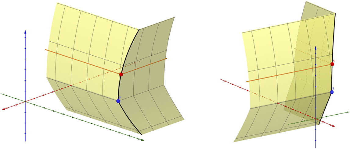
Figure 1 The image $j(B)=F(\mathscr Y)$
in
$j(B)=F(\mathscr Y)$
in $\mathbb R^{3}$
for
$\mathbb R^{3}$
for $n=2$
: It morally visualizes the integral affine structure.
$n=2$
: It morally visualizes the integral affine structure.
Sketch of proof of Theorem 1.5 omitting (iii).
Consider an analytic domain $\mathscr Y=\{ |x_1|<1\}$
in
$\mathscr Y=\{ |x_1|<1\}$
in $Y^{\mathrm {an}}$
. Define a topological embedding
$Y^{\mathrm {an}}$
. Define a topological embedding $j: \mathbb R^n \to \mathbb R^{n+1}$
assigning
$j: \mathbb R^n \to \mathbb R^{n+1}$
assigning $q=(q_1,\dots , q_{n-1}, q_n)=(\bar q,q_n)$
in
$q=(q_1,\dots , q_{n-1}, q_n)=(\bar q,q_n)$
in $\mathbb R^n$
to
$\mathbb R^n$
to
 $$\begin{align*}j(q)=(\min\{-\psi(q), -\psi(\bar q, 0) \}+\min\{0,\bar q\} \ , \ \min\{ \psi(q), \psi(\bar q,0) \} \ , \ \bar q). \end{align*}$$
Define a tropically continuous map $F:Y^{\mathrm {an}}\to \mathbb R^{n+1}$
by
$F:Y^{\mathrm {an}}\to \mathbb R^{n+1}$
by
 $$\begin{align*}F(x_0,x_1,y_1,\dots, y_{n-1})=(F_0,F_1, \operatorname{\mathrm{\mathsf{v}}}(y_1),\dots, \operatorname{\mathrm{\mathsf{v}}}(y_{n-1})), \end{align*}$$
where $\mathsf v:\Lambda \to \mathbb R\cup \{\infty \}$
is the non-archimedean valuation and
$\mathsf v:\Lambda \to \mathbb R\cup \{\infty \}$
is the non-archimedean valuation and
 $$\begin{align*}\begin{cases} F_0=\min \{ \operatorname{\mathrm{\mathsf{v}}}(x_0), -\psi(\operatorname{\mathrm{\mathsf{v}}}(y_1),\dots, \operatorname{\mathrm{\mathsf{v}}}(y_{n-1}),0)+\min\{0,\operatorname{\mathrm{\mathsf{v}}}(y_1),\dots, \operatorname{\mathrm{\mathsf{v}}}(y_{n-1})\}\} \\F_1=\min\{ \operatorname{\mathrm{\mathsf{v}}}(x_1), \ \ \ \psi (\operatorname{\mathrm{\mathsf{v}}}(y_1),\dots, \operatorname{\mathrm{\mathsf{v}}}(y_{n-1}),0)\}. \end{cases} \end{align*}$$
We can check $j(\mathbb R^n)=F(\mathscr Y)$
(cf. Figure 1). Then, we can define
$j(\mathbb R^n)=F(\mathscr Y)$
(cf. Figure 1). Then, we can define
 $$ \begin{align} f=j^{-1}\circ F|_{\mathscr Y} \ : \mathscr Y\to \mathbb R^n. \end{align} $$
This is a variant of [Reference Kontsevich and Soibelman50, §8] that further includes the data of the symplectic form; see also §3.3. By detailed calculations (Section 3.2.1 and Theorem 5.4), we will find that the smooth / singular loci and the induced integral affine structure of f
all
precisely agree with those of $\pi $
(2). Except the duality condition (iii), the proof is complete.
$\pi $
(2). Except the duality condition (iii), the proof is complete.
Remark 1.7. Here, we adopt the strategy of Kontsevich and Soibelman [Reference Kontsevich and Soibelman50, §8]. Rather than seeking the desired Berkovich-continuous map $f: \mathscr Y\to B$
, we find an alternative
$f: \mathscr Y\to B$
, we find an alternative $F:\mathscr Y\to \mathbb R^N$
for some larger N such that the image of F is identified with the singular integral affine manifold B through a map j. This embeds B into a larger Euclidean space
$F:\mathscr Y\to \mathbb R^N$
for some larger N such that the image of F is identified with the singular integral affine manifold B through a map j. This embeds B into a larger Euclidean space $\mathbb R^N$
to unfold the singularities (Figure 1). While this approach might seem ad-hoc for the singular part, the smooth part
$\mathbb R^N$
to unfold the singularities (Figure 1). While this approach might seem ad-hoc for the singular part, the smooth part $f_0\cong \pi _0^\vee $
remains canonical by the family Floer condition (iii). We hypothesize that the tropical continuity condition might ensure the uniqueness of the singular extension from
$f_0\cong \pi _0^\vee $
remains canonical by the family Floer condition (iii). We hypothesize that the tropical continuity condition might ensure the uniqueness of the singular extension from $f_0$
to f due to the piecewise-smooth nature of the reduced symplectic geometry, but this will be addressed in future work. Without the guidance from Floer theory, constructing the appropriate f is quite challenging. At least, directly replicating the example by Kontsevich-Soibelman seems difficult to match the singular integral affine structure from the Lagrangian fibration
$f_0$
to f due to the piecewise-smooth nature of the reduced symplectic geometry, but this will be addressed in future work. Without the guidance from Floer theory, constructing the appropriate f is quite challenging. At least, directly replicating the example by Kontsevich-Soibelman seems difficult to match the singular integral affine structure from the Lagrangian fibration $\pi $
, given its intricate dependence on the given symplectic form
$\pi $
, given its intricate dependence on the given symplectic form $\omega $
(cf. §1.2).
$\omega $
(cf. §1.2).
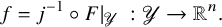
Figure 2 Two types of quantum corrections in red and yellow, meeting the singular fibers at the interior / boundary points of the disk domain respectively. The right side concerns the Lagrangian fibration $\pi $
in (2) for
$\pi $
in (2) for $n=2$
and follows Auroux [Reference Auroux5, 5.1].
$n=2$
and follows Auroux [Reference Auroux5, 5.1].
1.4 Outline of the construction
The existence of singular Lagrangian fibers may induce two types of quantum corrections of holomorphic disks as illustrated in red and yellow in Figure 2. The red disk meets the singular fiber at an interior point, while the yellow disk meets it at an boundary point. We will discuss the Floer aspect and the non-archimedean analytic aspect about them, respectively.
1.4.1 Floer aspect: dual affinoid torus fibration
Denote by $\pi _0:X_0\to B_0$
the smooth part of the Gross Lagrangian fibration
$\pi _0:X_0\to B_0$
the smooth part of the Gross Lagrangian fibration $\pi :X\to B$
. The non-archimedean dual torus fibration depends on the entire ambient space XX, as the disks may extend beyond the region
$\pi :X\to B$
. The non-archimedean dual torus fibration depends on the entire ambient space XX, as the disks may extend beyond the region $X_0=\pi ^{-1}(B_0)$
. By the Floer aspect of this type of quantum correction, we can canonically associate to
$X_0=\pi ^{-1}(B_0)$
. By the Floer aspect of this type of quantum correction, we can canonically associate to $(X,\pi _0)$
an analytic space
$(X,\pi _0)$
an analytic space $X_0^\vee $
with an abstract dual affinoid torus fibration
$X_0^\vee $
with an abstract dual affinoid torus fibration $\pi _0^\vee : X_0^\vee \to B_0$
(§4 or [Reference Yuan61]), unique up to isomorphism, so that its induced integral affine structure on
$\pi _0^\vee : X_0^\vee \to B_0$
(§4 or [Reference Yuan61]), unique up to isomorphism, so that its induced integral affine structure on $B_0$
agrees with the one induced by
$B_0$
agrees with the one induced by $\pi _0$
and the set of closed points in
$\pi _0$
and the set of closed points in $X_0^\vee $
are given by (1). Meanwhile, there is the other concrete affinoid torus fibration
$X_0^\vee $
are given by (1). Meanwhile, there is the other concrete affinoid torus fibration $f_0:\mathscr Y_0\to B_0$
(i.e., the smooth part of the analytic fibration f in (3)).
$f_0:\mathscr Y_0\to B_0$
(i.e., the smooth part of the analytic fibration f in (3)).
The initial step for our version of T-duality can be stated in a single relation as follows:
Proposition 1.8. There is an isomorphism of affinoid torus fibration $ \pi _0^\vee \cong f_0 $
.
$ \pi _0^\vee \cong f_0 $
.
The former $\pi _0^\vee $
is constructed canonically but abstractly, while the latter
$\pi _0^\vee $
is constructed canonically but abstractly, while the latter $f_0$
is ad hoc but concrete. We can even explicitly write down an analytic embedding
$f_0$
is ad hoc but concrete. We can even explicitly write down an analytic embedding $g:X_0^\vee \to \Lambda ^2\times (\Lambda ^*)^{n-1}$
with
$g:X_0^\vee \to \Lambda ^2\times (\Lambda ^*)^{n-1}$
with $\pi _0^\vee =f_0\circ g$
. The map g identifies
$\pi _0^\vee =f_0\circ g$
. The map g identifies $X_0^\vee $
with the analytic domain
$X_0^\vee $
with the analytic domain $\mathscr Y_0$
in Y. In view of (1), any closed point in
$\mathscr Y_0$
in Y. In view of (1), any closed point in $\mathscr Y_0$
can be realized as a local
$\mathscr Y_0$
can be realized as a local $U_\Lambda $
-system
$U_\Lambda $
-system $\mathbf y$
in some
$\mathbf y$
in some $H^1(L_q;U_\Lambda )$
. The explicit definition formula of g is in §5.4.
$H^1(L_q;U_\Lambda )$
. The explicit definition formula of g is in §5.4.

Remark 1.9. The
only
place we need the Floer theory is basically an identification between the family Floer mirror analytic space $X_0^\vee $
and an ‘adjunction’ analytic space
$X_0^\vee $
and an ‘adjunction’ analytic space $T_+\sqcup T_- /\sim $
obtained by gluing two analytic open domains
$T_+\sqcup T_- /\sim $
obtained by gluing two analytic open domains $T_\pm \subsetneq (\Lambda ^*)^n$
which correspond to the Clifford / Chekanov tori respectively (Remark 5.3). Such a simplification is not easy but now enables us to apply the idea in [Reference Gross, Hacking and Keel41, Lemma 3.1], where two copies of complex tori
$T_\pm \subsetneq (\Lambda ^*)^n$
which correspond to the Clifford / Chekanov tori respectively (Remark 5.3). Such a simplification is not easy but now enables us to apply the idea in [Reference Gross, Hacking and Keel41, Lemma 3.1], where two copies of complex tori $(\mathbb C^*)^n$
are glued instead; further combining the non-archimedean picture in [Reference Kontsevich and Soibelman50, p.44] enables us to discover the desired embedding g (see a reader guide in Remark 5.3.)
$(\mathbb C^*)^n$
are glued instead; further combining the non-archimedean picture in [Reference Kontsevich and Soibelman50, p.44] enables us to discover the desired embedding g (see a reader guide in Remark 5.3.)
Remark 1.10. The tropical polynomial $ \min \{0,q_1,\dots , q_{n-1}\} $
plays the leading roles in the singularities of both the A and B sides. First, the induced tropical hypersurface (i.e., the above minimum value attains at least twice) exactly describes the singular locus skeleton of the Gross Lagrangian fibration
$ \min \{0,q_1,\dots , q_{n-1}\} $
plays the leading roles in the singularities of both the A and B sides. First, the induced tropical hypersurface (i.e., the above minimum value attains at least twice) exactly describes the singular locus skeleton of the Gross Lagrangian fibration $\pi $
in (2). Second,
$\pi $
in (2). Second, $\operatorname {\mathrm {\mathsf {v}}}(1+y_1+\cdots +y_{n-1})$
is either
$\operatorname {\mathrm {\mathsf {v}}}(1+y_1+\cdots +y_{n-1})$
is either $>$
or
$>$
or $= \min \{0,\operatorname {\mathrm {\mathsf {v}}}(y_1),\dots , \operatorname {\mathrm {\mathsf {v}}}(y_{n-1})\}$
by the non-archimedean triangle inequality. The ambiguity case
$= \min \{0,\operatorname {\mathrm {\mathsf {v}}}(y_1),\dots , \operatorname {\mathrm {\mathsf {v}}}(y_{n-1})\}$
by the non-archimedean triangle inequality. The ambiguity case $>$
happens only if the minimum attains at least twice as well. After some effort, one may find that this ambiguity is the very reason of the singularity of f in (3). In general (§1.5), the desired dual map f is almost the same as (3) but using another tropical polynomial.
$>$
happens only if the minimum attains at least twice as well. After some effort, one may find that this ambiguity is the very reason of the singularity of f in (3). In general (§1.5), the desired dual map f is almost the same as (3) but using another tropical polynomial.
1.4.2 Non-archimedean analytic aspect: dual singular fibers
The significance of Proposition 1.8 lies on the fact that the abstract affinoid torus fibration $\pi _0^\vee : X_0^\vee \to B_0$
has an explicit model
$\pi _0^\vee : X_0^\vee \to B_0$
has an explicit model $f_0$
, via g, which naturally has an obvious tropically continuous extension f in (3) fitting in the diagram below.
$f_0$
, via g, which naturally has an obvious tropically continuous extension f in (3) fitting in the diagram below.

The left vertical arrow $\pi _0^\vee $
is the family Floer dual affinoid torus fibration
$\pi _0^\vee $
is the family Floer dual affinoid torus fibration $\pi _0^\vee $
in (iii). The upper horizontal map g follows Gross-Hacking-Keel in [Reference Gross, Hacking and Keel41, Lemma 3.1]. The right vertical arrow f generalizes Kontsevich-Soibelman’s singular model in [Reference Kontsevich and Soibelman50, §8]. Finally, the top right corner
$\pi _0^\vee $
in (iii). The upper horizontal map g follows Gross-Hacking-Keel in [Reference Gross, Hacking and Keel41, Lemma 3.1]. The right vertical arrow f generalizes Kontsevich-Soibelman’s singular model in [Reference Kontsevich and Soibelman50, §8]. Finally, the top right corner $\mathscr Y$
agrees with many previous results: [Reference Abouzaid, Auroux and Katzarkov1, Reference Abouzaid and Sylvan2, Reference Auroux5, Reference Auroux6, Reference Chan, Lau and Leung16, Reference Gammage37], etc.
$\mathscr Y$
agrees with many previous results: [Reference Abouzaid, Auroux and Katzarkov1, Reference Abouzaid and Sylvan2, Reference Auroux5, Reference Auroux6, Reference Chan, Lau and Leung16, Reference Gammage37], etc.
More importantly, the dual singular fibers do naturally capture the data of Lagrangian singular fibers. The other type of quantum correction refers to the holomorphic disks whose boundary meet the singular fibers (Figure 2, yellow), and they are all reflected by the formula of f (3). In summary, under the control of the canonical analytic structure on $(X_0^\vee , \pi _0^\vee )$
from the Floer aspect of the first type of quantum correction, the second type correction deduces the singular analytic extension. When we extend
$(X_0^\vee , \pi _0^\vee )$
from the Floer aspect of the first type of quantum correction, the second type correction deduces the singular analytic extension. When we extend $f_0$
to f tropically continuously [Reference Chambert-Loir and Ducros14, (3.1.6)], the topological extension
$f_0$
to f tropically continuously [Reference Chambert-Loir and Ducros14, (3.1.6)], the topological extension ![]() controls the analytic extension overhead (§3.2). Note that any affinoid torus fibration is tropically continuous.
controls the analytic extension overhead (§3.2). Note that any affinoid torus fibration is tropically continuous.
Our explicit description of the f in (3) can depict all the dual singular fibers simultaneously, and the general results in §1.5 will even offer more local models of SYZ singularities. The aspects of non-archimedean analytic topology seem to outweigh the Floer-theoretic considerations around the singular locus $\Delta =B\setminus B_0$
. Moreover, we will astonishingly discover in the set level that (see §5.6)
$\Delta =B\setminus B_0$
. Moreover, we will astonishingly discover in the set level that (see §5.6)
 $$ \begin{align} \text{Dual singular fiber} \ \ \supsetneq \ \ \text{Maurer-Cartan set of the singular fiber} \end{align} $$
based on the work of Hong-Kim-Lau [Reference Hong, Kim and Lau45]. This justifies our standpoint in [Reference Yuan61] that going beyond the usual Maurer-Cartan picture [Reference Fukaya32, Reference Fukaya34, Reference Tu59] is necessary to produce the global mirror analytic structure. A well-known fact in the area of homological algebra is that the homotopy equivalences among $A_\infty $
algebras induce bijections of Maurer-Cartan sets. However, this offers merely a local or set-theoretic approximation and is not sufficient for the local-to-global construction of a non-archimedean analytic space. By definition, the latter is built by matching the affinoid spaces instead.
$A_\infty $
algebras induce bijections of Maurer-Cartan sets. However, this offers merely a local or set-theoretic approximation and is not sufficient for the local-to-global construction of a non-archimedean analytic space. By definition, the latter is built by matching the affinoid spaces instead.
1.5 Main result in general
Our method is very powerful in that the same ideas for Theorem 1.5 with some basics of tropical and toric geometry can obtain more general results with very little extra effort.
Denote by N and M two lattices of rank n that are dual to each other. Set $N_{\mathbb R}=N\otimes \mathbb R$
and
$N_{\mathbb R}=N\otimes \mathbb R$
and $M_{\mathbb R}=M\otimes \mathbb R$
. Let
$M_{\mathbb R}=M\otimes \mathbb R$
. Let $\Sigma $
be a simplicial smooth fan with maximal cones n-dimensional in
$\Sigma $
be a simplicial smooth fan with maximal cones n-dimensional in $N_{\mathbb R}$
. Assume
$N_{\mathbb R}$
. Assume $v_1,\dots , v_n$
are the primitive generators of the rays in a maximal cone in
$v_1,\dots , v_n$
are the primitive generators of the rays in a maximal cone in $\Sigma $
, so they form a
$\Sigma $
, so they form a $\mathbb Z$
-basis of N. Denote by
$\mathbb Z$
-basis of N. Denote by $v_1^*,\dots , v_n^*$
the dual basis of M. Denote the remaining rays in
$v_1^*,\dots , v_n^*$
the dual basis of M. Denote the remaining rays in $\Sigma $
by
$\Sigma $
by $v_{n+1},\dots , v_{n+r}$
for
$v_{n+1},\dots , v_{n+r}$
for $r\ge 0$
, and we set
$r\ge 0$
, and we set $v_{n+a}=\sum _{j=1}^n k_{aj} v_j$
for
$v_{n+a}=\sum _{j=1}^n k_{aj} v_j$
for $k_{aj}\in \mathbb Z$
and
$k_{aj}\in \mathbb Z$
and $1\le a\le r$
. Assume the toric variety
$1\le a\le r$
. Assume the toric variety $\mathcal X_\Sigma $
associated to
$\mathcal X_\Sigma $
associated to $\Sigma $
is Calabi-Yau; namely, there exists
$\Sigma $
is Calabi-Yau; namely, there exists $m_0\in M$
so that
$m_0\in M$
so that $\langle m_0,v\rangle =1$
for any ray v in
$\langle m_0,v\rangle =1$
for any ray v in $\Sigma $
. Then,
$\Sigma $
. Then, $m_0=v_1^*+\cdots +v_n^*$
and
$m_0=v_1^*+\cdots +v_n^*$
and $\sum _{j=1}^n k_{aj}=1$
for any
$\sum _{j=1}^n k_{aj}=1$
for any $1\le a \le r$
. Let
$1\le a \le r$
. Let $w=z^{m_0}$
be the toric character associated to
$w=z^{m_0}$
be the toric character associated to $m_0$
, and
$m_0$
, and $ \mathscr D:=\{w=1\} $
is an anti-canonical divisor in
$ \mathscr D:=\{w=1\} $
is an anti-canonical divisor in $\mathcal X_\Sigma $
. We equip
$\mathcal X_\Sigma $
. We equip $\mathcal X_\Sigma $
with a toric Kähler form
$\mathcal X_\Sigma $
with a toric Kähler form $\omega $
, and the moment map
$\omega $
, and the moment map $\mu : \mathcal X_\Sigma \to M_{\mathbb R}$
is onto a polyhedral P described by a collection of inequalities as follows:
$\mu : \mathcal X_\Sigma \to M_{\mathbb R}$
is onto a polyhedral P described by a collection of inequalities as follows:
 $$ \begin{align} P: \quad \langle m, v_i\rangle +\lambda_i\ge 0 \qquad m\in M_{\mathbb R}, \end{align} $$
where the $v_i$
’s run over all the rays in
$v_i$
’s run over all the rays in $\Sigma $
and
$\Sigma $
and $\lambda _i\in \mathbb R$
. The sublattice
$\lambda _i\in \mathbb R$
. The sublattice $\bar N=\{ n\in N\mid \langle m_0,n\rangle =0\}$
has a basis
$\bar N=\{ n\in N\mid \langle m_0,n\rangle =0\}$
has a basis $\sigma _s=v_s-v_n$
for
$\sigma _s=v_s-v_n$
for $1\le s<n$
. The action of
$1\le s<n$
. The action of $\bar N\otimes \mathbb C^*$
preserves
$\bar N\otimes \mathbb C^*$
preserves $\mathscr D$
and gives a moment map
$\mathscr D$
and gives a moment map $\bar \mu $
onto
$\bar \mu $
onto $\bar M_{\mathbb R}:=M_{\mathbb R}/\mathbb Rm_0$
such that
$\bar M_{\mathbb R}:=M_{\mathbb R}/\mathbb Rm_0$
such that $p\circ \mu =\bar \mu $
for the projection
$p\circ \mu =\bar \mu $
for the projection $p: M_{\mathbb R}\to \bar M_{\mathbb R}$
. One can show p induces a homeomorphism
$p: M_{\mathbb R}\to \bar M_{\mathbb R}$
. One can show p induces a homeomorphism $\partial P\cong \bar M_{\mathbb R}$
. We identify
$\partial P\cong \bar M_{\mathbb R}$
. We identify $\bar M_{\mathbb R}:=M_{\mathbb R}/\mathbb Rm_0$
with a copy of
$\bar M_{\mathbb R}:=M_{\mathbb R}/\mathbb Rm_0$
with a copy of $\mathbb R^{n-1}$
in
$\mathbb R^{n-1}$
in $M_{\mathbb R}\cong \mathbb R^n$
consisting of
$M_{\mathbb R}\cong \mathbb R^n$
consisting of $(m_1,\dots , m_n)$
with
$(m_1,\dots , m_n)$
with $m_n=0$
. Now, the Gross special Lagrangian fibration [Reference Gross39] refers to
$m_n=0$
. Now, the Gross special Lagrangian fibration [Reference Gross39] refers to $\pi :=(\bar \mu , \log |w-1|)$
on
$\pi :=(\bar \mu , \log |w-1|)$
on $ X:=\mathcal X_\Sigma \setminus \mathscr D $
(see also [Reference Abouzaid, Auroux and Katzarkov1, Reference Chan, Lau and Leung16]). The singular locus of
$ X:=\mathcal X_\Sigma \setminus \mathscr D $
(see also [Reference Abouzaid, Auroux and Katzarkov1, Reference Chan, Lau and Leung16]). The singular locus of $\pi $
takes the form
$\pi $
takes the form $\Delta =\Pi \times \{0\}$
, where
$\Delta =\Pi \times \{0\}$
, where $\Pi $
is the tropical hypersurface (Figure 3) in
$\Pi $
is the tropical hypersurface (Figure 3) in $\bar M_{\mathbb R}\cong \mathbb R^{n-1}$
associated to the tropical polynomial that is decided by the data in (7):
$\bar M_{\mathbb R}\cong \mathbb R^{n-1}$
associated to the tropical polynomial that is decided by the data in (7):
 $$ \begin{align} h_{\mathrm{trop}}(q_1,\dots, q_{n-1})= \min\Big\{ \lambda_n, \{q_k+\lambda_k\}_{1\le k<n}, \{\textstyle \sum_{s=1}^{n-1}k_{as}q_s+\lambda_{n+a}\}_{1\le a\le r} \Big\}. \end{align} $$
Recall that the Novikov field $\Lambda =\mathbb C((T^{\mathbb R}))$
is algebraically closed. Let
$\Lambda =\mathbb C((T^{\mathbb R}))$
is algebraically closed. Let $\Lambda _0$
and
$\Lambda _0$
and $\Lambda _+$
be the valuation ring and its maximal ideal. However, given the A side data above, we consider
$\Lambda _+$
be the valuation ring and its maximal ideal. However, given the A side data above, we consider
 $$ \begin{align} h(y_1,\dots, y_{n-1})= T^{\lambda_n}(1+\delta_n) + \sum_{s=1}^{n-1}T^{\lambda_s} y_s (1+\delta_s) + \sum_a T^{\lambda_{n+a}} (1+\delta_{n+a}) \prod_{s=1}^{n-1} y_s^{k_{as}}, \end{align} $$
where $\delta _i\in \Lambda _+$
is given by some virtual counts so that
$\delta _i\in \Lambda _+$
is given by some virtual counts so that $\mathsf v(\delta _i)$
is the smallest symplectic area of the sphere bubbles meeting the toric divisor
$\mathsf v(\delta _i)$
is the smallest symplectic area of the sphere bubbles meeting the toric divisor $D_i$
associated to
$D_i$
associated to $v_i$
(see §6 for the details).
$v_i$
(see §6 for the details).
Remark 1.11. In general, the Cho-Oh’s result [Reference Cho and Oh21] is not enough to decide the $\delta _i$
’s. But, whenever
$\delta _i$
’s. But, whenever $D_i$
is non-compact, one can use the maximal principle to show that
$D_i$
is non-compact, one can use the maximal principle to show that $\delta _i=0$
(cf. [Reference Chan, Lau and Leung16, §5.2]). The expressions of
$\delta _i=0$
(cf. [Reference Chan, Lau and Leung16, §5.2]). The expressions of $\delta _i$
may be also interpreted via the inverse mirror maps due to [Reference Chan, Cho, Lau and Tseng15].
$\delta _i$
may be also interpreted via the inverse mirror maps due to [Reference Chan, Cho, Lau and Tseng15].


A key observation is that the tropicalization of h in (9) is precisely $h_{\mathrm {trop}}$
in (8), since
$h_{\mathrm {trop}}$
in (8), since $\delta _i\in \Lambda _+$
. This picture is lost if we only work over
$\delta _i\in \Lambda _+$
. This picture is lost if we only work over $\mathbb C$
. By Definition 1.4, let’s state a more general result:
$\mathbb C$
. By Definition 1.4, let’s state a more general result:
Theorem 1.12. The algebraic variety
 $$\begin{align*}Y=\{(x_0,x_1,y_1,\dots, y_{n-1})\in \Lambda^2\times (\Lambda^*)^{n-1} \mid x_0x_1= h(y_1,\dots, y_{n-1}) \} \end{align*}$$
is SYZ mirror to $X=\mathcal X_\Sigma \setminus \mathscr D$
.
$X=\mathcal X_\Sigma \setminus \mathscr D$
.
The proof is almost identical to that of Theorem 1.5. The key dual singular fibration f is written in the same way as (3), replacing the tropical polynomial $\min \{0,q_1,\dots , q_{n-1}\}$
by
$\min \{0,q_1,\dots , q_{n-1}\}$
by $h_{\mathrm {trop}}$
(Remark 1.10). So, for legibility, we focus on Theorem 1.5 in the main body and delay the generalization to §6.
$h_{\mathrm {trop}}$
(Remark 1.10). So, for legibility, we focus on Theorem 1.5 in the main body and delay the generalization to §6.
1.6 Examples and SYZ converse
The statement of Theorem 1.12 gives rise to a lot of examples.
1.6.1
We begin with a general remark for a version of SYZ converse. One can use the Laurent polynomial h to recover the polyhedral P as follows. Consider the polyhedral $P'$
in
$P'$
in $\bar M_{\mathbb R}\oplus \mathbb R\cong \mathbb R^{n-1}\oplus \mathbb R$
defined by
$\bar M_{\mathbb R}\oplus \mathbb R\cong \mathbb R^{n-1}\oplus \mathbb R$
defined by $ q_n+h_{\mathrm {trop}}(q_1,\dots ,q_{n-1})\ge 0 $
. Namely, it is defined by
$ q_n+h_{\mathrm {trop}}(q_1,\dots ,q_{n-1})\ge 0 $
. Namely, it is defined by $q_n+\lambda _n\ge 0$
,
$q_n+\lambda _n\ge 0$
, $q_n+q_s+\lambda _s\ge 0$
(
$q_n+q_s+\lambda _s\ge 0$
( $1\le s<n$
), and
$1\le s<n$
), and $q_n+\sum _{s=1}^{n-1} k_{as}q_s+\lambda _{n+a}\ge 0$
(
$q_n+\sum _{s=1}^{n-1} k_{as}q_s+\lambda _{n+a}\ge 0$
( $1\le a\le r$
) due to (8). Then, the isomorphism
$1\le a\le r$
) due to (8). Then, the isomorphism $\bar M_{\mathbb R}\oplus \mathbb R\cong M_{\mathbb R}$
,
$\bar M_{\mathbb R}\oplus \mathbb R\cong M_{\mathbb R}$
, $(q_1,\dots , q_{n-1},q_n)\mapsto (q_1+q_n,\dots , q_{n-1}+q_n, q_n)$
, can naturally identify
$(q_1,\dots , q_{n-1},q_n)\mapsto (q_1+q_n,\dots , q_{n-1}+q_n, q_n)$
, can naturally identify $P'$
with P in (7).
$P'$
with P in (7).
1.6.2
Back to Theorem 1.5, we have $r=0$
,
$r=0$
, $\lambda _i=0$
, and
$\lambda _i=0$
, and $\delta _i=0$
. Then, by (9),
$\delta _i=0$
. Then, by (9), $h=1+y_1+\cdots +y_{n-1}$
, and its tropicalization is
$h=1+y_1+\cdots +y_{n-1}$
, and its tropicalization is $h_{\mathrm {trop}}=\min \{0,q_1,\dots , q_{n-1}\}$
; see Figure 3. Compare also Remark 1.10. We can also check the polyhedral
$h_{\mathrm {trop}}=\min \{0,q_1,\dots , q_{n-1}\}$
; see Figure 3. Compare also Remark 1.10. We can also check the polyhedral $P'\cong P$
is identified with the first quadrant in
$P'\cong P$
is identified with the first quadrant in $\mathbb R^n$
.
$\mathbb R^n$
.
1.6.3
Consider the fan $\Sigma $
in
$\Sigma $
in $\mathbb R^3$
generated by
$\mathbb R^3$
generated by $v_1=(1,0,0)$
,
$v_1=(1,0,0)$
, $v_2=(0,1,0)$
,
$v_2=(0,1,0)$
, $v_3=(0,0,1)$
, and
$v_3=(0,0,1)$
, and $v_4=(1,-1,1)$
. So,
$v_4=(1,-1,1)$
. So, $n=3$
and
$n=3$
and $r=1$
. Note that
$r=1$
. Note that $v_4=v_1-v_2+v_3$
(i.e.,
$v_4=v_1-v_2+v_3$
(i.e., $k_{11}=k_{13}=1$
and
$k_{11}=k_{13}=1$
and $k_{12}=-1$
). The corresponding toric variety is the conifold
$k_{12}=-1$
). The corresponding toric variety is the conifold $\mathcal X_\Sigma =\mathcal O_{\mathbb P^1}(-1)\oplus \mathcal O_{\mathbb P^1}(-1)$
. We equip
$\mathcal X_\Sigma =\mathcal O_{\mathbb P^1}(-1)\oplus \mathcal O_{\mathbb P^1}(-1)$
. We equip $\mathcal X_\Sigma $
with a toric Kähler form
$\mathcal X_\Sigma $
with a toric Kähler form $\omega $
, and the moment polyhedral P is defined by (7) for some arbitrary
$\omega $
, and the moment polyhedral P is defined by (7) for some arbitrary $\lambda _1,\dots , \lambda _4\in \mathbb R$
. By (9),
$\lambda _1,\dots , \lambda _4\in \mathbb R$
. By (9), $h(y_1,y_2)=T^{\lambda _3} +T^{\lambda _1}y_1+T^{\lambda _2}y_2+T^{\lambda _4} y_1 y_2^{-1}$
. First, we may assume
$h(y_1,y_2)=T^{\lambda _3} +T^{\lambda _1}y_1+T^{\lambda _2}y_2+T^{\lambda _4} y_1 y_2^{-1}$
. First, we may assume $\lambda _3=0$
. Also, replacing
$\lambda _3=0$
. Also, replacing $y_i$
by
$y_i$
by $T^{-\lambda _i}y_i$
, we may assume
$T^{-\lambda _i}y_i$
, we may assume $\lambda _1=\lambda _2=0$
. So,
$\lambda _1=\lambda _2=0$
. So, $(\lambda _1,\lambda _2,\lambda _3,\lambda _4)=(0,0,0, \lambda )$
for some
$(\lambda _1,\lambda _2,\lambda _3,\lambda _4)=(0,0,0, \lambda )$
for some $\lambda \in \mathbb R$
, and
$\lambda \in \mathbb R$
, and $h=1+y_1+y_2+T^\lambda y_1y_2^{-1}$
. This retrieves the case of [Reference Chan, Lau and Leung16, 5.3.2] if we replace the Novikov parameter T by some
$h=1+y_1+y_2+T^\lambda y_1y_2^{-1}$
. This retrieves the case of [Reference Chan, Lau and Leung16, 5.3.2] if we replace the Novikov parameter T by some $t\in \mathbb C$
. But, we remark that the shapes of the tropical hypersurfaces of
$t\in \mathbb C$
. But, we remark that the shapes of the tropical hypersurfaces of $h_{\mathrm {trop}}$
or the moment polyhedrals
$h_{\mathrm {trop}}$
or the moment polyhedrals $P'\cong P$
obtained by §1.6.1 are different for
$P'\cong P$
obtained by §1.6.1 are different for $\lambda>0$
and
$\lambda>0$
and $\lambda <0$
, which seems lost over
$\lambda <0$
, which seems lost over $\mathbb C$
.
$\mathbb C$
.
1.6.4
Consider the Laurent polynomial $h(y_1,y_2)=y_1+T^{-1}y_2+T^{3.14}+T^2y_1^2+y_1y_2+T^2y_2^2$
. By §1.6.1, we get the fan
$h(y_1,y_2)=y_1+T^{-1}y_2+T^{3.14}+T^2y_1^2+y_1y_2+T^2y_2^2$
. By §1.6.1, we get the fan $\Sigma $
in
$\Sigma $
in $\mathbb R^3$
generated by
$\mathbb R^3$
generated by $v_1=(1,0,0)$
,
$v_1=(1,0,0)$
, $v_2=(0,1,0)$
,
$v_2=(0,1,0)$
, $v_3=(0,0,1)$
,
$v_3=(0,0,1)$
, $v_4=(2,0,-1)$
,
$v_4=(2,0,-1)$
, $v_5=(1,1,-1)$
,
$v_5=(1,1,-1)$
, $v_6=(0,2,-1)$
. Also, we get the polyhedral P defined by (7) with respect to these
$v_6=(0,2,-1)$
. Also, we get the polyhedral P defined by (7) with respect to these $v_i$
’s and the numbers
$v_i$
’s and the numbers $\lambda _1=0$
,
$\lambda _1=0$
, $\lambda _2=-1$
,
$\lambda _2=-1$
, $\lambda _3=3.14$
,
$\lambda _3=3.14$
, $\lambda _4=2$
,
$\lambda _4=2$
, $\lambda _5=0$
,
$\lambda _5=0$
, $\lambda _6=2$
. Note that the above h is carefully chosen so that the tropical hypersurface associated to
$\lambda _6=2$
. Note that the above h is carefully chosen so that the tropical hypersurface associated to $h_{\mathrm {trop}}$
does not enclose a bounded region (Figure 3, right). This ensures the toric variety
$h_{\mathrm {trop}}$
does not enclose a bounded region (Figure 3, right). This ensures the toric variety $\mathcal X_\Sigma $
has no compact irreducible toric divisor (cf. Remark 1.11). By Theorem 1.12 and §1.6.1, we achieve a version of SYZ converse construction from B side to A side. Notice that we truly have infinitely many such examples.
$\mathcal X_\Sigma $
has no compact irreducible toric divisor (cf. Remark 1.11). By Theorem 1.12 and §1.6.1, we achieve a version of SYZ converse construction from B side to A side. Notice that we truly have infinitely many such examples.
1.7 Further evidence: a folklore conjecture
We have extra evidence supporting our proposed SYZ statement for the following folklore conjecture, recognized by Auroux, Kontsevich and Seidel [Reference Auroux5, §6]:
Conjecture II. The critical values of the mirror Landau-Ginzburg superpotential on $X^\vee $
(B side) are the eigenvalues of the quantum multiplication by the first Chern class on X (A side).
$X^\vee $
(B side) are the eigenvalues of the quantum multiplication by the first Chern class on X (A side).
Recall the dual affinoid torus fibration $\pi _0^\vee :X_0^\vee \to B_0$
only relies on the Maslov-0 holomorphic disks in X bounded by
$\pi _0^\vee :X_0^\vee \to B_0$
only relies on the Maslov-0 holomorphic disks in X bounded by $\pi _0$
-fibers. It often happens that the
$\pi _0$
-fibers. It often happens that the $\pi _0$
can be placed in a larger ambient space
$\pi _0$
can be placed in a larger ambient space $\overline X$
, adding more Maslov-2 holomorphic disks but adding no Maslov-0 ones. By the general theory in [Reference Yuan61], the family Floer mirror associated to the same fibration
$\overline X$
, adding more Maslov-2 holomorphic disks but adding no Maslov-0 ones. By the general theory in [Reference Yuan61], the family Floer mirror associated to the same fibration $\pi _0$
, placed in the larger
$\pi _0$
, placed in the larger $\overline X$
yet, is given by the same analytic space
$\overline X$
yet, is given by the same analytic space $X_0^\vee $
and the same affinoid torus fibration
$X_0^\vee $
and the same affinoid torus fibration $\pi _0^\vee : X_0^\vee \to B_0$
but equipped with an additional function
$\pi _0^\vee : X_0^\vee \to B_0$
but equipped with an additional function $W_0^\vee $
on
$W_0^\vee $
on $X_0^\vee $
(§4.6). Note that the
$X_0^\vee $
(§4.6). Note that the $W_0^\vee $
as well as its critical points and critical values all depend on the Kähler form
$W_0^\vee $
as well as its critical points and critical values all depend on the Kähler form $\omega $
. When we deform
$\omega $
. When we deform $\omega $
, the image of these critical points under the fibration map
$\omega $
, the image of these critical points under the fibration map $\pi $
may wildly change. But, in the present paper, we only focus on the examples and refer to [Reference Yuan62] for the general theory.
$\pi $
may wildly change. But, in the present paper, we only focus on the examples and refer to [Reference Yuan62] for the general theory.
Recall $\mathscr Y_0=f_0^{-1}(B_0)\cong X_0^\vee $
via the analytic embedding g in (4). In our case, the LG superpotential turns out to be polynomial, and from Definition 1.4, it follows that
$\mathscr Y_0=f_0^{-1}(B_0)\cong X_0^\vee $
via the analytic embedding g in (4). In our case, the LG superpotential turns out to be polynomial, and from Definition 1.4, it follows that $\mathscr Y_0$
is Zariski dense in the algebraic variety Y (cf. [Reference Payne55]). Thus, the
$\mathscr Y_0$
is Zariski dense in the algebraic variety Y (cf. [Reference Payne55]). Thus, the $W_0^\vee $
extends to a polynomial superpotential
$W_0^\vee $
extends to a polynomial superpotential $W^\vee $
on the whole Y. Note that the
$W^\vee $
on the whole Y. Note that the $W^\vee $
relies on the larger ambient space
$W^\vee $
relies on the larger ambient space $\overline X$
, although the Y does not. For various ambient spaces
$\overline X$
, although the Y does not. For various ambient spaces $\overline X$
, we have various
$\overline X$
, we have various $W^\vee $
. The computations in [Reference Yuan63] over the Novikov field
$W^\vee $
. The computations in [Reference Yuan63] over the Novikov field $\Lambda = \mathbb C((T^{\mathbb R}))$
rather than just over
$\Lambda = \mathbb C((T^{\mathbb R}))$
rather than just over $\mathbb C$
(e.g., [Reference Pascaleff and Tonkonog54]) are quite crucial to verify Conjecture II here. The details of computations will be in Appendix §A, and we just write down the results here:
$\mathbb C$
(e.g., [Reference Pascaleff and Tonkonog54]) are quite crucial to verify Conjecture II here. The details of computations will be in Appendix §A, and we just write down the results here:
-
1. Suppose
$X=\mathbb C^n\setminus \{z_1\cdots z_n=1\}$
and
$\overline X=\mathbb {CP}^n$
. Then, the LG superpotential is defined on the algebraic variety
$$\begin{align*}W^\vee = x_1+\frac{T^{E(\mathcal H)} x_0^n}{ y_1\cdots y_{n-1}} \end{align*}$$
$Y=\{x_0x_1=1+y_1+\cdots +y_{n-1}\}$
, where
$\mathcal H$
is the class of a complex line and
$E(\mathcal H)=\frac {1}{2\pi }\omega \cap \mathcal H$
is the symplectic area. By direct computations, one can check the critical points of this
$W^\vee $
(for the logarithmic derivatives) are
$$\begin{align*}\begin{cases} x_0 = T^{-\frac{E(\mathcal H)}{n+1}} e^{-\frac{2\pi i s}{n+1}} & \\ x_1 = n T^{\frac{E(\mathcal H)}{n+1} } e^{\frac{2\pi i s}{n+1}} & \\ y_1=\cdots=y_{n-1}=1 \end{cases} \qquad s\in\{0,1,\dots, n\}, \end{align*}$$
They are all contained in the same dual fiber over the base point that can be in either the Clifford or Chekanov chambers, relying on
$\omega $
and
$\pi $
. Moreover, one can check the critical values are which agrees with the
$$\begin{align*}(n+1) T^{\frac{E(\mathcal H)}{n+1}} e^{\frac{2\pi i s}{n+1}}, \qquad s\in\{0,1,\dots, n\}, \end{align*}$$
$c_1$
-eigenvalues in the quantum cohomology
$QH^*(\mathbb {CP}^n; \Lambda )$
.
-
2. Suppose
$X=\mathbb C^n\setminus \{z_1\cdots z_n=1\}$
and
$\overline X=\mathbb {CP}^m\times \mathbb {CP}^{n-m}$
for
$0<m<n$
. Then, on the same Y, where
$$\begin{align*}W^\vee = x_1 + \frac{T^{E(\mathcal H_1)} x_0^m}{y_1\cdots y_m} + \frac{T^{E(\mathcal H_2)} x_0^{n-m}}{ y_{m+1}\cdots y_{n-1}} \end{align*}$$
$\mathcal H_1, \mathcal H_2$
are the classes of a complex line in
$\mathbb {CP}^m$
and
$\mathbb {CP}^{n-m}$
, respectively. The corresponding critical values are for
$$\begin{align*}(m+1) T^{\frac{E(\mathcal H_1)}{m+1}} e^{\frac{2\pi i r}{m+1}} + (n-m+1) T^{\frac{E(\mathcal H_2)}{n-m+1}} e^{\frac{2\pi i s}{n-m+1}} \end{align*}$$
$r\in \{0,1,\dots , m\}$
and
$s\in \{0,1,\dots , n-m\}$
and agree with the
$c_1$
-eigenvalues. Moreover, we want to further study the locations of the critical points of
$W^\vee $
. For simplicity, let’s assume
$n=2$
and
$m=1$
. Then
$ W^\vee =x_1+ \frac {T^{E(\mathcal H_1)} x_0}{y} +T^{E(\mathcal H_2)} x_0 $
is defined on
$Y=\{x_0x_1=1+y\}$
. We have four critical points of
$W^\vee $
given by
$$\begin{align*}\begin{cases} x_0=\pm T^{\frac{-E(\mathcal H_2)}{2}} \\ x_1= \pm T^{\frac{E(\mathcal H_1)}{2}} \pm T^{\frac{E(\mathcal H_2)}{2}} \\ y_1= \pm T^{\frac{E(\mathcal H_1)-E(\mathcal H_2)}{2}}. \end{cases} \end{align*}$$
They are contained in the f-fiber over the base point
$ \hat q=\left (\frac {E(\mathcal H_1)-E(\mathcal H_2)}{2}, a_\omega \right ) $
in
$B\equiv \mathbb R^2$
, where
$a_\omega $
is some value that relies on the Kähler form
$\omega $
.


We really obtain infinitely many LG superpotentials on Y parameterized by the various Kähler forms, and all of them will satisfy the folklore conjecture. In the case (2) above, it may happen that $E(\mathcal H_1)\neq E(\mathcal H_2)$
while
$E(\mathcal H_1)\neq E(\mathcal H_2)$
while $a_\omega =0$
; then the base point
$a_\omega =0$
; then the base point $\hat q$
meets the wall. In general, the base points of critical points rely on
$\hat q$
meets the wall. In general, the base points of critical points rely on $\omega $
or
$\omega $
or $\pi $
, and the walls of Maslov-0 disks rely on J. The family Floer non-archimedean analytic structure does not rely on J up to isomorphism [Reference Yuan61]. For instance, the formula of f in (3) clearly does not rely on J and cannot detect the walls of Maslov-0 disks (relying on J). To sum up, the Maslov-0 correction is usually unavoidable (cf. [Reference Auroux7, §5] [Reference Auroux6, Example 3.3.2]) and gives rise to some non-archimedean analytic structure which needs to be remembered in the Floer theory along the way. Given nontrivial Maslov-0 disks, all the previous arguments for Conjecture II will fail. A major new challenge is that the LG superpotential is now locally only well-defined up to affinoid algebra isomorphisms, or more precisely up to family Floer transition maps in the language of [Reference Yuan61]. Fortunately, based on the ud-homotopy and canceling tricks in [Reference Yuan61], a conceptual proof of Conjecture II with Maslov-0 corrections has been achieved in [Reference Yuan62]. Admittedly, its value may rely on future examples we would find, but there are clearly other examples by Theorem 1.12 with similar computations. The new ideas in [Reference Yuan62] will also inspire future studies, such as a more global picture of the closed-string mirror symmetry that asserts the quantum cohomology of X is isomorphic to the Jacobian ring of
$\pi $
, and the walls of Maslov-0 disks rely on J. The family Floer non-archimedean analytic structure does not rely on J up to isomorphism [Reference Yuan61]. For instance, the formula of f in (3) clearly does not rely on J and cannot detect the walls of Maslov-0 disks (relying on J). To sum up, the Maslov-0 correction is usually unavoidable (cf. [Reference Auroux7, §5] [Reference Auroux6, Example 3.3.2]) and gives rise to some non-archimedean analytic structure which needs to be remembered in the Floer theory along the way. Given nontrivial Maslov-0 disks, all the previous arguments for Conjecture II will fail. A major new challenge is that the LG superpotential is now locally only well-defined up to affinoid algebra isomorphisms, or more precisely up to family Floer transition maps in the language of [Reference Yuan61]. Fortunately, based on the ud-homotopy and canceling tricks in [Reference Yuan61], a conceptual proof of Conjecture II with Maslov-0 corrections has been achieved in [Reference Yuan62]. Admittedly, its value may rely on future examples we would find, but there are clearly other examples by Theorem 1.12 with similar computations. The new ideas in [Reference Yuan62] will also inspire future studies, such as a more global picture of the closed-string mirror symmetry that asserts the quantum cohomology of X is isomorphic to the Jacobian ring of $W^\vee $
(cf. [Reference Fukaya, Oh, Ohta and Ono36]).
$W^\vee $
(cf. [Reference Fukaya, Oh, Ohta and Ono36]).
2 A side: the Gross Lagrangian fibration
2.1 Lagrangian fibration
We begin with the Gross’s construction in [Reference Gross39]. Define the divisors $D_j=\{z_j=0\}$
(
$D_j=\{z_j=0\}$
( $1\le \ell \le n$
) and
$1\le \ell \le n$
) and $\mathscr D=\{z_1z_2\cdots z_n=1\}$
in
$\mathscr D=\{z_1z_2\cdots z_n=1\}$
in $\mathbb C^n$
. We set
$\mathbb C^n$
. We set $X=\mathbb C^n\setminus \mathscr D$
. Consider the
$X=\mathbb C^n\setminus \mathscr D$
. Consider the $T^{n-1}$
-action given by
$T^{n-1}$
-action given by
 $$ \begin{align} t \cdot (z_1,\dots, z_n) \mapsto (z_1,\dots, z_{k-1}, e^{it} z_k, z_{k+1},\dots, z_{n-1}, e^{-it} z_n) \qquad 1\le k<n \end{align} $$
for $t\in S^1\cong \mathbb R/2\pi \mathbb Z$
. Take the standard symplectic form
$t\in S^1\cong \mathbb R/2\pi \mathbb Z$
. Take the standard symplectic form $\omega =d\lambda $
on
$\omega =d\lambda $
on $\mathbb C^n$
. Let
$\mathbb C^n$
. Let $ \bar \mu =(h_1,\dots , h_{n-1}): \mathbb C^n\to \mathbb R^{n-1} $
be a moment map for the
$ \bar \mu =(h_1,\dots , h_{n-1}): \mathbb C^n\to \mathbb R^{n-1} $
be a moment map for the $T^{n-1}$
-action in (10). One can check the vector fields
$T^{n-1}$
-action in (10). One can check the vector fields
 $$\begin{align*}\textstyle \mathfrak X_k= i \big(\bar z_k\frac{\partial}{\partial\bar z_k } - z_k\frac{\partial}{\partial z_k}\big) - i \big(\bar z_n\frac{\partial}{\partial\bar z_n } - z_n\frac{\partial}{\partial z_n}\big) \end{align*}$$
satisfy $ \iota (\mathfrak X_k)\omega = d h_k $
for the Hamiltonian functions
$ \iota (\mathfrak X_k)\omega = d h_k $
for the Hamiltonian functions
 $$\begin{align*}h_k(z)=\tfrac{1}{2} \big(|z_k|^2- |z_n|^2 \big) \qquad 1\le k<n. \end{align*}$$
Define $h_n(z)=\log |z_1\cdots z_n-1|$
and
$h_n(z)=\log |z_1\cdots z_n-1|$
and $B=\mathbb R^n$
. The Gross Lagrangian fibration (with respect to the holomorphic n-form
$B=\mathbb R^n$
. The Gross Lagrangian fibration (with respect to the holomorphic n-form $\Omega =(z_1\cdots z_n-1)^{-1} dz_1\wedge \cdots \wedge dz_n$
, cf. [Reference Gross39]) refers to the following:
$\Omega =(z_1\cdots z_n-1)^{-1} dz_1\wedge \cdots \wedge dz_n$
, cf. [Reference Gross39]) refers to the following:
 $$\begin{align*}\pi\equiv (\bar\mu, h_n): X \to B, \quad (z_1,\dots, z_n)\mapsto \big( h_1,\dots, h_{n-1} , h_n \big). \end{align*}$$
Note that the $\pi $
maps X onto B. Note also that the
$\pi $
maps X onto B. Note also that the $\pi $
-fibers are preserved by the complex conjugation
$\pi $
-fibers are preserved by the complex conjugation $z_i\mapsto \bar z_i$
. The
$z_i\mapsto \bar z_i$
. The $\pi $
-fiber over
$\pi $
-fiber over $q\in B$
is denoted by
$q\in B$
is denoted by $L_q:=\pi ^{-1}(q)$
, and we write
$L_q:=\pi ^{-1}(q)$
, and we write
 $$\begin{align*}q=(\bar q, q_n)=(q_1,\dots, q_{n-1},q_n) \end{align*}$$
for the standard Euclidean coordinates in $B \equiv \mathbb R^n$
. Let
$B \equiv \mathbb R^n$
. Let $ P_{ij}=\{z_i=z_j=0\}=D_i\cap D_j $
and
$ P_{ij}=\{z_i=z_j=0\}=D_i\cap D_j $
and $\Delta _{ij}=\pi (P_{ij})$
. The discriminant locus of
$\Delta _{ij}=\pi (P_{ij})$
. The discriminant locus of $\pi $
is precisely
$\pi $
is precisely $\Delta =\bigcup \Delta _{ij}$
, and the smooth locus of
$\Delta =\bigcup \Delta _{ij}$
, and the smooth locus of $\pi $
is
$\pi $
is $B_0:=B\setminus \Delta $
. We denote the restriction of
$B_0:=B\setminus \Delta $
. We denote the restriction of $\pi $
over
$\pi $
over $B_0$
by
$B_0$
by
 $$\begin{align*}\pi_0:=\pi|_{B_0} :X_0\to B_0 \end{align*}$$
where $X_0:=\pi _0^{-1}(B_0)\subset X$
. Moreover, we actually have
$X_0:=\pi _0^{-1}(B_0)\subset X$
. Moreover, we actually have $\Delta =\Pi \times \{0\}$
, where
$\Delta =\Pi \times \{0\}$
, where $\Pi $
is the tropical hyperplane that consists of those
$\Pi $
is the tropical hyperplane that consists of those $\bar q \in \mathbb R^{n-1}$
such that
$\bar q \in \mathbb R^{n-1}$
such that $\min \{0,q_1,\dots , q_{n-1}\}$
is attained twice. The tropical hyperplane
$\min \{0,q_1,\dots , q_{n-1}\}$
is attained twice. The tropical hyperplane $\Pi $
separates the subset
$\Pi $
separates the subset $H: =(\mathbb R^{n-1}\setminus \Pi )\times \{0\}$
of the base B into n different connected components
$H: =(\mathbb R^{n-1}\setminus \Pi )\times \{0\}$
of the base B into n different connected components
 $$ \begin{align} H_k= \{ \bar q \in \mathbb R^{n-1}\setminus \Pi \mid \min (0,q_1,\dots, q_{n-1})=q_k\} \end{align} $$
for $1\le k<n$
and
$1\le k<n$
and
 $$\begin{align*}H_n=\{ \bar q \in\mathbb R^{n-1}\setminus \Pi \mid \min(0,q_1,\dots, q_{n-1}) =0\}. \end{align*}$$
For example, when $n{\kern-1pt}={\kern-1pt}3$
, we have
$n{\kern-1pt}={\kern-1pt}3$
, we have $H_1{\kern-1.2pt}={\kern-1.2pt}\{q_1{\kern-1.2pt}<{\kern-1.2pt}0, q_1{\kern-1.2pt}<{\kern-1.2pt}q_2\}$
,
$H_1{\kern-1.2pt}={\kern-1.2pt}\{q_1{\kern-1.2pt}<{\kern-1.2pt}0, q_1{\kern-1.2pt}<{\kern-1.2pt}q_2\}$
, $H_2{\kern-1.2pt}={\kern-1.2pt}\{q_2{\kern-1.2pt}<{\kern-1.2pt}0, q_1{\kern-1.2pt}>{\kern-1.2pt}q_2\}$
and
$H_2{\kern-1.2pt}={\kern-1.2pt}\{q_2{\kern-1.2pt}<{\kern-1.2pt}0, q_1{\kern-1.2pt}>{\kern-1.2pt}q_2\}$
and $H_3{\kern-1.2pt}={\kern-1.2pt}\{q_1{\kern-1.2pt}>{\kern-1.2pt}0, q_2{\kern-1.2pt}>{\kern-1.2pt}0\}$
(see the left side of Figure 3). When
$H_3{\kern-1.2pt}={\kern-1.2pt}\{q_1{\kern-1.2pt}>{\kern-1.2pt}0, q_2{\kern-1.2pt}>{\kern-1.2pt}0\}$
(see the left side of Figure 3). When $n=2$
, we have
$n=2$
, we have $H_1=(-\infty , 0)$
and
$H_1=(-\infty , 0)$
and $H_2=(0,+\infty )$
. Notice that
$H_2=(0,+\infty )$
. Notice that $\bar H_i\cap \bar H_j=\Delta _{ij}=\pi (D_i\cap D_j)$
, and
$\bar H_i\cap \bar H_j=\Delta _{ij}=\pi (D_i\cap D_j)$
, and $H_j\subset \pi (D_j)$
for
$H_j\subset \pi (D_j)$
for $1\le j\le n$
.
$1\le j\le n$
.
We usually call the subset H in $B_0$
the wall because a torus fiber
$B_0$
the wall because a torus fiber $L_q$
over
$L_q$
over $q=(\bar q, q_n)\in B_0$
bounds a nontrivial Maslov index zero holomorphic disk if and only if
$q=(\bar q, q_n)\in B_0$
bounds a nontrivial Maslov index zero holomorphic disk if and only if $q_n=0$
(i.e.,
$q_n=0$
(i.e., $q\in H$
) (see, for example [Reference Auroux6, Example 3.3.1] or [Reference Auroux5, §5]). Next, we define
$q\in H$
) (see, for example [Reference Auroux6, Example 3.3.1] or [Reference Auroux5, §5]). Next, we define
 $$\begin{align*}B_+=\{q=(q_1,\dots, q_n )\mid q_n>0\}=\mathbb R^{n-1}\times (0,+\infty) \end{align*}$$
 $$\begin{align*}B_-=\{q=(q_1, \dots, q_n)\mid q_n<0\} =\mathbb R^{n-1}\times (-\infty,0). \end{align*}$$
Then, $B_0=B_+ \sqcup B_-\sqcup \bigsqcup _{j=1}^n H_j$
. We call the
$B_0=B_+ \sqcup B_-\sqcup \bigsqcup _{j=1}^n H_j$
. We call the $B_+$
(resp.
$B_+$
(resp. $B_-$
) the chamber of Clifford tori (resp. Chekanov tori). We say the torus fiber
$B_-$
) the chamber of Clifford tori (resp. Chekanov tori). We say the torus fiber $L_q$
is of Clifford type if
$L_q$
is of Clifford type if $q_n>0$
and it is of Chekanov type if
$q_n>0$
and it is of Chekanov type if $q_n<0$
, which is introduced in [Reference Chekanov17, Reference Eliashberg and Polterovich27] and many others.
$q_n<0$
, which is introduced in [Reference Chekanov17, Reference Eliashberg and Polterovich27] and many others.
The Arnold-Liouville’s theorem implies the existence of the action-angle coordinates near any Lagrangian torus fiber. Let $(M,\omega )$
be a symplectic manifold of dimension
$(M,\omega )$
be a symplectic manifold of dimension $2n$
. Let
$2n$
. Let $M_U\subset M$
be an open subset. The following two theorems are standard; see [Reference Duistermaat24] and [Reference Evans28].
$M_U\subset M$
be an open subset. The following two theorems are standard; see [Reference Duistermaat24] and [Reference Evans28].
Theorem 2.1. Let $\pi =(H_1,\dots , H_n) : M_U \to U$
be an integrable Hamiltonian system over a contractible domain U with only smooth torus fibers. Then, there exists a diffeomorphism
$\pi =(H_1,\dots , H_n) : M_U \to U$
be an integrable Hamiltonian system over a contractible domain U with only smooth torus fibers. Then, there exists a diffeomorphism $\chi : U \to V\subset \mathbb R^n$
such that
$\chi : U \to V\subset \mathbb R^n$
such that $\chi \circ \pi $
generates a Hamiltonian torus action on M. In other words, there is a local coordinate system
$\chi \circ \pi $
generates a Hamiltonian torus action on M. In other words, there is a local coordinate system $(I, \alpha )=(I_1,\dots , I_n,\alpha _1,\dots ,\alpha _n): \pi ^{-1}(U) \to U\times (\mathbb R/ 2\pi \mathbb Z)^n$
such that
$(I, \alpha )=(I_1,\dots , I_n,\alpha _1,\dots ,\alpha _n): \pi ^{-1}(U) \to U\times (\mathbb R/ 2\pi \mathbb Z)^n$
such that $I=\chi \circ \pi $
and
$I=\chi \circ \pi $
and $\omega =\sum _{i=1}^n dI_i\wedge d\alpha _i$
on
$\omega =\sum _{i=1}^n dI_i\wedge d\alpha _i$
on $\pi ^{-1}(U)$
.
$\pi ^{-1}(U)$
.
We call $I=(I_1,\dots , I_n)$
and
$I=(I_1,\dots , I_n)$
and $\alpha =(\alpha _1,\dots ,\alpha _n)$
the action-angle coordinates. Two sets of them differ by an integral affine transformation. If
$\alpha =(\alpha _1,\dots ,\alpha _n)$
the action-angle coordinates. Two sets of them differ by an integral affine transformation. If $\pi :M_U\to U$
is a smooth Lagrangian torus fibration in
$\pi :M_U\to U$
is a smooth Lagrangian torus fibration in $M_U\subset M$
over a contractible domain U, then a set of the action coordinates is decided by a choice of the
$M_U\subset M$
over a contractible domain U, then a set of the action coordinates is decided by a choice of the $\mathbb Z$
-basis of
$\mathbb Z$
-basis of $H_1(\pi ^{-1}(q); \mathbb Z)$
for some
$H_1(\pi ^{-1}(q); \mathbb Z)$
for some $q\in U$
. In reality, we have the following.
$q\in U$
. In reality, we have the following.
Theorem 2.2. Let $\lambda $
be some 1-form in
$\lambda $
be some 1-form in $M_U$
such that
$M_U$
such that $\omega =d\lambda $
. Assume
$\omega =d\lambda $
. Assume $\sigma _i=\sigma _i(q)$
are closed curves in the torus fiber
$\sigma _i=\sigma _i(q)$
are closed curves in the torus fiber $\pi ^{-1}(q)\cong T^n$
, depending smoothly on q, such that they form a basis in
$\pi ^{-1}(q)\cong T^n$
, depending smoothly on q, such that they form a basis in $H_1(\pi ^{-1}(q); \mathbb Z)$
. Then
$H_1(\pi ^{-1}(q); \mathbb Z)$
. Then $\psi _i= \frac {1}{2\pi } \int _{\sigma _i} \lambda $
defines a diffeomorphism
$\psi _i= \frac {1}{2\pi } \int _{\sigma _i} \lambda $
defines a diffeomorphism $\chi =(\psi _1,\dots ,\psi _n):U\to \mathbb R^n$
such that a set of action coordinates on
$\chi =(\psi _1,\dots ,\psi _n):U\to \mathbb R^n$
such that a set of action coordinates on $M_U$
are given by
$M_U$
are given by $I_i=\psi _i\circ \pi $
.
$I_i=\psi _i\circ \pi $
.
We will call such a $\chi $
an integral affine chart. If we pick a different
$\chi $
an integral affine chart. If we pick a different $\lambda '$
with
$\lambda '$
with $d\lambda '=d\lambda $
, then by Stokes’ theorem,
$d\lambda '=d\lambda $
, then by Stokes’ theorem, $\int _{\sigma _i}(\lambda '-\lambda )$
is constant, and the action coordinates just differ by constants. The
$\int _{\sigma _i}(\lambda '-\lambda )$
is constant, and the action coordinates just differ by constants. The $\psi _i$
’s in Theorem 2.2 are also called the flux maps. The formula for a set of action coordinates can be complicated in general (cf. [Reference Ngoc60], see also [Reference Evans28, Theorem 6.7]). A key idea used in this paper is that the action coordinates can be often described by linear combinations of symplectic areas of disks in some (possibly larger) ambient space; see §2.3 below. The advantage is that one can intuitively see an integral affine transformation in terms of disk bubbling.
$\psi _i$
’s in Theorem 2.2 are also called the flux maps. The formula for a set of action coordinates can be complicated in general (cf. [Reference Ngoc60], see also [Reference Evans28, Theorem 6.7]). A key idea used in this paper is that the action coordinates can be often described by linear combinations of symplectic areas of disks in some (possibly larger) ambient space; see §2.3 below. The advantage is that one can intuitively see an integral affine transformation in terms of disk bubbling.
2.2 Topological disks
Now, we go back to our situation. To connect with the Floer theory, we are interested in whether the loops in $\pi _1(L_q)$
can be realized as (linear combinations of) the boundaries of disks in
$\pi _1(L_q)$
can be realized as (linear combinations of) the boundaries of disks in $X=\mathbb C^n\setminus \mathscr D$
or in other reasonable larger ambient symplectic manifold
$X=\mathbb C^n\setminus \mathscr D$
or in other reasonable larger ambient symplectic manifold $\overline X$
(e.g.,
$\overline X$
(e.g., $\mathbb C^n$
or
$\mathbb C^n$
or $\mathbb {CP}^n$
). Beware that at this moment, we just focus on topological disks rather than holomorphic disks. We consider the following local systems over
$\mathbb {CP}^n$
). Beware that at this moment, we just focus on topological disks rather than holomorphic disks. We consider the following local systems over $B_0$
:
$B_0$
:
 $$ \begin{align} \mathscr R_1:=R^1\pi_*(\mathbb Z)\equiv \bigcup_{q\in B_0} \pi_1(L_q), \qquad \mathscr R_2 :=\mathscr R_2(\overline X):=\bigcup_{q\in B_0} \pi_2( \overline X,L_q). \end{align} $$
We must understand the monodromy behavior of the above local systems across multiple components of the walls (cf. Figure 3). In contrast, most of existing literature only studies these disks across a single component. Although the latter is sufficient for mirror space identifications (cf. [Reference Abouzaid, Auroux and Katzarkov1, Reference Chan, Lau and Leung16] and §1.2), we must understand the former monodromy data for mirror fibration realizations. Note also that the monodromy for $\mathscr R_2$
contains more information than the monodromy for
$\mathscr R_2$
contains more information than the monodromy for $\mathscr R_1$
or the integral affine structure. This justifies why we need to provide many additional details here, although it may be not so difficult.
$\mathscr R_1$
or the integral affine structure. This justifies why we need to provide many additional details here, although it may be not so difficult.
The local system $\mathscr R_2=\mathscr R_2(\overline X)$
generally depends on the ambient space
$\mathscr R_2=\mathscr R_2(\overline X)$
generally depends on the ambient space $\overline X$
. But, we will often make this point implicit. Taking the boundaries gives rise to a morphism
$\overline X$
. But, we will often make this point implicit. Taking the boundaries gives rise to a morphism $\partial : \mathscr R_2\to \mathscr R_1$
. A class in
$\partial : \mathscr R_2\to \mathscr R_1$
. A class in $\pi _1(L_q)$
or
$\pi _1(L_q)$
or $\pi _2(\overline X,L_q)$
determines a local section of
$\pi _2(\overline X,L_q)$
determines a local section of $\mathscr R_1$
or
$\mathscr R_1$
or $\mathscr R_2$
over some contractible domain that contains q. Recall that we have a natural Hamiltonian
$\mathscr R_2$
over some contractible domain that contains q. Recall that we have a natural Hamiltonian $T^{n-1}$
-action that preserves the Lagrangian torus fibers. Then, for
$T^{n-1}$
-action that preserves the Lagrangian torus fibers. Then, for $q\in B_0$
, we use
$q\in B_0$
, we use $\sigma _k=\sigma _k(q)$
(
$\sigma _k=\sigma _k(q)$
( $1\le k\le n-1$
) to denote the class of the orbit of the
$1\le k\le n-1$
) to denote the class of the orbit of the $S^1$
-action in (10). They can be regarded as the global sections of
$S^1$
-action in (10). They can be regarded as the global sections of $\mathscr R_1$
.
$\mathscr R_1$
.
To avoid the monodromy ambiguity, we will work with a covering of the base manifold $B_0$
by the contractible domains, such as
$B_0$
by the contractible domains, such as $B_+\cup H_\ell \cup B_-$
for
$B_+\cup H_\ell \cup B_-$
for $1\le \ell \le n$
. Let
$1\le \ell \le n$
. Let $\mathscr N_\ell $
denote a sufficiently small neighborhood of
$\mathscr N_\ell $
denote a sufficiently small neighborhood of $H_\ell $
in the smooth locus
$H_\ell $
in the smooth locus $B_0$
. The following two contractible domains can cover
$B_0$
. The following two contractible domains can cover $B_0$
:
$B_0$
:
 $$\begin{align*}\textstyle B^{\prime}_\pm := B_\pm \cup \bigsqcup_{\ell=1}^n \mathscr N_\ell. \end{align*}$$
Whenever $q\in B_+$
, the Lagrangian torus fiber
$q\in B_+$
, the Lagrangian torus fiber $L_q$
can deform into a product torus by a Hamiltonian isotopy inside
$L_q$
can deform into a product torus by a Hamiltonian isotopy inside $(\mathbb C^*)^n$
. So,
$(\mathbb C^*)^n$
. So, $\pi _2(\mathbb C^n, L_q)\cong \pi _2(\mathbb C^n, (\mathbb C^*)^n )\cong \mathbb Z^n$
has an obvious basis
$\pi _2(\mathbb C^n, L_q)\cong \pi _2(\mathbb C^n, (\mathbb C^*)^n )\cong \mathbb Z^n$
has an obvious basis $\beta _1,\dots ,\beta _n$
such that
$\beta _1,\dots ,\beta _n$
such that $\beta _i\cdot D_j=\delta _{ij}$
. We can represent
$\beta _i\cdot D_j=\delta _{ij}$
. We can represent $\partial \beta _j$
by a loop in the form
$\partial \beta _j$
by a loop in the form $t\mapsto (z_1^0,\dots , z_j^0 e^{it},\dots , z_n^0)$
in the product torus. But abusing the notations, we still write
$t\mapsto (z_1^0,\dots , z_j^0 e^{it},\dots , z_n^0)$
in the product torus. But abusing the notations, we still write $\partial \beta _j$
(resp.
$\partial \beta _j$
(resp. $\beta _j$
) for the induced local sections of
$\beta _j$
) for the induced local sections of $\mathscr R_1$
(resp.
$\mathscr R_1$
(resp. $\mathscr R_2$
) over
$\mathscr R_2$
) over $B^{\prime }_+$
. To emphasize the base point, we may write
$B^{\prime }_+$
. To emphasize the base point, we may write $\partial \beta _j(q)$
and
$\partial \beta _j(q)$
and $\beta _j(q)$
. By (10), we have
$\beta _j(q)$
. By (10), we have
 $$ \begin{align} \sigma_k|_{B^{\prime}_+}= \partial\beta_k -\partial\beta_n \qquad 1\le k<n. \end{align} $$
However, there is a preferred local section of $\mathscr R_2$
over
$\mathscr R_2$
over $B_-$
, denoted by
$B_-$
, denoted by $ \hat \beta : B_- \to \mathscr R_2 $
, such that any Maslov index 2 holomorphic disk u bounding
$ \hat \beta : B_- \to \mathscr R_2 $
, such that any Maslov index 2 holomorphic disk u bounding $L_{q}$
for
$L_{q}$
for $q\in B_-$
must have
$q\in B_-$
must have $[u]=\hat \beta (q)$
; see, for example, [Reference Eliashberg and Polterovich27, Proposition 4.2. C], [Reference Chan, Lau and Leung16, Lemma 4.31] or [Reference Yuan63]. It can be represented by a section of
$[u]=\hat \beta (q)$
; see, for example, [Reference Eliashberg and Polterovich27, Proposition 4.2. C], [Reference Chan, Lau and Leung16, Lemma 4.31] or [Reference Yuan63]. It can be represented by a section of $z_1\cdots z_n$
over a disk in
$z_1\cdots z_n$
over a disk in $\mathbb C$
. Note that
$\mathbb C$
. Note that $\hat \beta \cdot D_i=0$
for all i. Abusing the notation, we still denote by
$\hat \beta \cdot D_i=0$
for all i. Abusing the notation, we still denote by $\hat \beta $
the extension section of
$\hat \beta $
the extension section of $\mathscr R_2$
over
$\mathscr R_2$
over $B^{\prime }_-$
. By studying the intersection numbers with the various divisors, it is direct to show the following purely topological result (see, for example, [Reference Yuan63, Lemma B.7]):
$B^{\prime }_-$
. By studying the intersection numbers with the various divisors, it is direct to show the following purely topological result (see, for example, [Reference Yuan63, Lemma B.7]):
 $$ \begin{align} \beta_\ell|_{\mathscr N_\ell}=\hat\beta|_{\mathscr N_\ell}. \end{align} $$
Convention 2.3.
From now on, we will adopt a slightly different convention compared to our previous works [Reference Yuan61, Reference Yuan62, Reference Yuan63]: We define $E(\beta )=\frac {1}{2\pi } \omega \cap \beta $
instead of
$E(\beta )=\frac {1}{2\pi } \omega \cap \beta $
instead of $E(\beta )=\omega \cap \beta $
for
$E(\beta )=\omega \cap \beta $
for $\beta \in \pi _2(X,L)$
.
$\beta \in \pi _2(X,L)$
.
2.3 Action coordinates
Recall that $ q=(q_1,\dots , q_n)=:(\bar q, q_n) $
are the standard coordinates on B, but we aim to find the different action coordinates. On the one hand, a natural trivialization of
$ q=(q_1,\dots , q_n)=:(\bar q, q_n) $
are the standard coordinates on B, but we aim to find the different action coordinates. On the one hand, a natural trivialization of $\mathscr R_1|_{B^{\prime }_-}$
is given by the sections
$\mathscr R_1|_{B^{\prime }_-}$
is given by the sections
 $$\begin{align*}\{\sigma_k|_{B^{\prime}_-}: 1\le k<n \}\cup \{\partial\hat\beta\}. \end{align*}$$
By Theorem 2.2, they give rise to a set of the action coordinates in $B^{\prime }_-$
by the flux maps. The first
$B^{\prime }_-$
by the flux maps. The first $n-1$
fluxes are given by
$n-1$
fluxes are given by $ \frac {1}{2\pi } \int _{\sigma _k} \lambda = \frac {1}{2} ( |z_k|^2- |z_n|^2 ) = h_k(z)=q_k $
. The last flux for
$ \frac {1}{2\pi } \int _{\sigma _k} \lambda = \frac {1}{2} ( |z_k|^2- |z_n|^2 ) = h_k(z)=q_k $
. The last flux for $\partial \hat \beta =\partial \hat \beta (q)$
is hard to make explicit, but it can have a geometric meaning by the Stokes’ formula:
$\partial \hat \beta =\partial \hat \beta (q)$
is hard to make explicit, but it can have a geometric meaning by the Stokes’ formula:
 $$\begin{align*}\textstyle \psi_-(q):=\frac{1}{2\pi} \int_{\partial\hat\beta} \lambda =\frac{1}{2\pi} \int_{\hat\beta} d\lambda= E(\hat\beta), \end{align*}$$
which is regarded as a map $\psi _-: B^{\prime }_-\to \mathbb R$
. To sum up, we get an integral affine coordinate chart
$\psi _-: B^{\prime }_-\to \mathbb R$
. To sum up, we get an integral affine coordinate chart
 $$ \begin{align} \chi_- : B^{\prime}_- \to \mathbb R^n ,\qquad q\mapsto (q_1,\dots, q_{n-1}, \psi_-(q) ) = (\bar q, \psi_-(q)). \end{align} $$
On the other hand, a natural trivialization of $\mathscr R_1|_{B^{\prime }_+}$
is given by
$\mathscr R_1|_{B^{\prime }_+}$
is given by
 $$\begin{align*}\{\sigma_k|_{B^{\prime}_+}: 1\le k<n\} \cup\{\partial\beta_n\}. \end{align*}$$
Recall that $\sigma _k|_{B^{\prime }_+}=\partial \beta _k-\partial \beta _n$
for
$\sigma _k|_{B^{\prime }_+}=\partial \beta _k-\partial \beta _n$
for $1\le k<n$
. The first
$1\le k<n$
. The first $n-1$
fluxes are as above, and moreover,
$n-1$
fluxes are as above, and moreover,
 $$ \begin{align} \textstyle E(\beta_k) - E(\beta_n) = \frac{1}{2\pi} \int_{\beta_k-\beta_n} d\lambda =\frac{1}{2\pi} \int_{\partial\beta_k-\partial\beta_n} \lambda= \frac{1}{2\pi } \int_{\sigma_k} \lambda = q_k. \end{align} $$
Define $ \psi _+(q)= E(\beta _n): B^{\prime }_+\to \mathbb R $
. By Theorem 2.2, the associated integral affine coordinate chart is
$ \psi _+(q)= E(\beta _n): B^{\prime }_+\to \mathbb R $
. By Theorem 2.2, the associated integral affine coordinate chart is
 $$ \begin{align} \chi_+ : B^{\prime}_+ \to \mathbb R^n, \qquad q \mapsto \big(q_1, \dots, q_{n-1}, \psi_+(q) \big) = (\bar q, \psi_+(q)). \end{align} $$
We can use (14) and (16) to conclude that $\psi _+(q)=\psi _-(q)$
on
$\psi _+(q)=\psi _-(q)$
on $\mathscr N_n$
and
$\mathscr N_n$
and $\psi _+(q)+q_\ell =\psi _-(q)$
on
$\psi _+(q)+q_\ell =\psi _-(q)$
on $\mathscr N_\ell $
for
$\mathscr N_\ell $
for $\ell \neq n$
, respectively. By (11), this means that for
$\ell \neq n$
, respectively. By (11), this means that for $ \textstyle q\in B^{\prime }_+\cap B^{\prime }_-\equiv \bigsqcup _\ell \mathscr N_\ell $
,
$ \textstyle q\in B^{\prime }_+\cap B^{\prime }_-\equiv \bigsqcup _\ell \mathscr N_\ell $
,
 $$ \begin{align} \psi_-(q) = \psi_+(q)+\min\{0,q_1,\dots, q_{n-1}\}. \end{align} $$
The two charts $\chi _\pm $
give rise to an integral affine structure on
$\chi _\pm $
give rise to an integral affine structure on $B_0$
which is different from the standard Euclidean one in
$B_0$
which is different from the standard Euclidean one in $B=\mathbb R^n$
. In particular, the former integral affine structure cannot be extended to B. Define
$B=\mathbb R^n$
. In particular, the former integral affine structure cannot be extended to B. Define $ \unicode{x3c7} _\ell :=\chi _-\circ \chi _+^{-1}: \ \chi _+(\mathscr N_\ell ) \to \chi _-(\mathscr N_\ell ) $
for each
$ \unicode{x3c7} _\ell :=\chi _-\circ \chi _+^{-1}: \ \chi _+(\mathscr N_\ell ) \to \chi _-(\mathscr N_\ell ) $
for each $\ell $
, and we can check
$\ell $
, and we can check
2.4 The embedding j
We aim to embed the integral affine manifold with singularities B into a higher-dimensional Euclidean space $\mathbb R^{n+1}$
. This is actually inspired by the work of Kontsevich-Soibelman (cf. [Reference Kontsevich and Soibelman50, p27 & p45]). To some degree, this helps us to visualize the integral affine structure.
$\mathbb R^{n+1}$
. This is actually inspired by the work of Kontsevich-Soibelman (cf. [Reference Kontsevich and Soibelman50, p27 & p45]). To some degree, this helps us to visualize the integral affine structure.
2.4.1 Symplectic area
Thanks to (18), we have a well-defined continuous function on $B_0$
given by
$B_0$
given by
 $$ \begin{align} \psi(q)=\psi(\bar q, q_n) = \begin{cases} \psi_+(q)+\min\{0,q_1,\dots, q_{n-1}\}, & q\in B^{\prime}_+ \\ \psi_-(q) , & q\in B^{\prime}_-. \end{cases} \end{align} $$
If $q\in B^{\prime }_+$
, then
$q\in B^{\prime }_+$
, then $\psi (q)=\min \{E(\beta _1),\dots , E(\beta _n)\}$
; if
$\psi (q)=\min \{E(\beta _1),\dots , E(\beta _n)\}$
; if $q\in B^{\prime }_-$
, then
$q\in B^{\prime }_-$
, then $\psi (q)=E(\hat \beta )$
. The existence of the Lagrangian fibration with singularities over the whole
$\psi (q)=E(\hat \beta )$
. The existence of the Lagrangian fibration with singularities over the whole $B=\mathbb R^n$
tells that the
$B=\mathbb R^n$
tells that the $\psi $
can extend continuously from
$\psi $
can extend continuously from $B_0$
to B, still denoted by
$B_0$
to B, still denoted by $\psi : B \to \mathbb R $
(cf. the yellow disks in Figure 2). The value of
$\psi : B \to \mathbb R $
(cf. the yellow disks in Figure 2). The value of $\psi (q)$
can be represented by the symplectic area of a topological disk
$\psi (q)$
can be represented by the symplectic area of a topological disk
 $$\begin{align*}u=u(q): (\mathbb D, \partial\mathbb D) \to (\mathbb C^n, L_q) \end{align*}$$
by $\psi (q)= \frac {1}{2\pi } \int u^*\omega $
(cf. Convention 2.3). It is not necessarily a holomorphic disk at this moment, and the symplectic area is purely topological.
$\psi (q)= \frac {1}{2\pi } \int u^*\omega $
(cf. Convention 2.3). It is not necessarily a holomorphic disk at this moment, and the symplectic area is purely topological.
Lemma 2.4. The function $q_n\mapsto \psi (\bar q, q_n)$
is an increasing diffeomorphism from
$q_n\mapsto \psi (\bar q, q_n)$
is an increasing diffeomorphism from $\mathbb R$
to
$\mathbb R$
to $(0,\infty )$
.
$(0,\infty )$
.
Proof. We first show the monotonicity. We may assume that $\bar q$
is a regular value of
$\bar q$
is a regular value of $\bar \mu $
(otherwise, since we only compare the symplectic areas, we may take a sequence of regular values approaching it). We study the symplectic reduction space
$\bar \mu $
(otherwise, since we only compare the symplectic areas, we may take a sequence of regular values approaching it). We study the symplectic reduction space $\Sigma :=\bar \mu ^{-1}(\bar q) / T^{n-1}$
. It has real dimension 2 and is endowed with the reduction form
$\Sigma :=\bar \mu ^{-1}(\bar q) / T^{n-1}$
. It has real dimension 2 and is endowed with the reduction form $\omega _{red}$
. If we write
$\omega _{red}$
. If we write ![]() and
and $p: \bar \mu ^{-1}(\bar q) \to \Sigma $
for the inclusion and quotient maps, then
$p: \bar \mu ^{-1}(\bar q) \to \Sigma $
for the inclusion and quotient maps, then $i^*\omega =p^*\omega _{red}$
. The Lefschetz fibration map
$i^*\omega =p^*\omega _{red}$
. The Lefschetz fibration map $w=z_1\cdots z_n$
is invariant under the
$w=z_1\cdots z_n$
is invariant under the $T^{n-1}$
action and naturally induces a diffeomorphism
$T^{n-1}$
action and naturally induces a diffeomorphism $v: \Sigma \to \mathbb C$
with
$v: \Sigma \to \mathbb C$
with $w\circ i=v\circ p$
. Note that
$w\circ i=v\circ p$
. Note that $L_q$
is contained in
$L_q$
is contained in $\bar \mu ^{-1}(\bar q)$
, and the topological disk u is a section of w. Up to a homotopy in
$\bar \mu ^{-1}(\bar q)$
, and the topological disk u is a section of w. Up to a homotopy in $\mathbb C^n$
(relative to
$\mathbb C^n$
(relative to $L_q$
), we may require u has its image contained in
$L_q$
), we may require u has its image contained in $\bar \mu ^{-1}(\bar q)$
as well. Recall
$\bar \mu ^{-1}(\bar q)$
as well. Recall $h_n=\log | w-1|$
, so
$h_n=\log | w-1|$
, so $|w-1|=e^{q_n}$
on
$|w-1|=e^{q_n}$
on $L_q$
. Now, we have the following maps of topological space-pairs:
$L_q$
. Now, we have the following maps of topological space-pairs:
 $$\begin{align*}(\mathbb D, \partial\mathbb D) \xrightarrow{u} (\bar\mu^{-1}(\bar q), L_q) \xrightarrow{p} (\Sigma, p(L_q) ) \xrightarrow[\cong]{v} (\mathbb C, \partial D(q_n)), \end{align*}$$
where $p(L_q)$
is identified via v with the boundary circle of the disk
$p(L_q)$
is identified via v with the boundary circle of the disk $D(q_n)=\{\zeta \in \mathbb C\mid |\zeta -1|\le e^{q_n}\}$
. Let
$D(q_n)=\{\zeta \in \mathbb C\mid |\zeta -1|\le e^{q_n}\}$
. Let $\check \omega $
is a symplectic form on
$\check \omega $
is a symplectic form on $\mathbb C$
determined by
$\mathbb C$
determined by $v^*\check \omega =\omega _{red}$
. Then,
$v^*\check \omega =\omega _{red}$
. Then, $\int u^*\omega = \int u^* p^*\omega _{red} = \int u^* p^* v^* \check \omega $
. In other words,
$\int u^*\omega = \int u^* p^*\omega _{red} = \int u^* p^* v^* \check \omega $
. In other words, $2\pi \psi (q)=\int u^*\omega $
can be viewed as the symplectic area of the disk
$2\pi \psi (q)=\int u^*\omega $
can be viewed as the symplectic area of the disk $D(q_n)$
in
$D(q_n)$
in $(\mathbb C, \check \omega )$
. No matter how
$(\mathbb C, \check \omega )$
. No matter how $\check \omega $
looks like, we have the subset inclusion
$\check \omega $
looks like, we have the subset inclusion $D(q^1_n)\subset D(q^2_n)$
if
$D(q^1_n)\subset D(q^2_n)$
if $q^1_n<q^2_n$
, so the
$q^1_n<q^2_n$
, so the $\check \omega $
-area of
$\check \omega $
-area of $D(q_n)$
is increasing in
$D(q_n)$
is increasing in $q_n$
. Namely, this says
$q_n$
. Namely, this says $\psi (\bar q,q_n)$
is increasing in
$\psi (\bar q,q_n)$
is increasing in $q_n$
. Finally, notice that we also have
$q_n$
. Finally, notice that we also have $\lim _{q_n\to \infty } \psi (\bar q, q_n)=\infty $
and
$\lim _{q_n\to \infty } \psi (\bar q, q_n)=\infty $
and $\lim _{q_n\to -\infty }\psi (\bar q, q_n)=0$
.
$\lim _{q_n\to -\infty }\psi (\bar q, q_n)=0$
.
Recall that $q=(\bar q, q_n)$
. We write
$q=(\bar q, q_n)$
. We write
 $$ \begin{align} \psi_0(\bar q)=\psi(\bar q,0), \end{align} $$
and we define a continuous embedding
 $$ \begin{align} j: B \to \mathbb R^{n+1} \qquad q\mapsto (\theta_0(q), \ \theta_1(q), \ \bar q ), \end{align} $$
where
 $$ \begin{align} \begin{aligned} \theta_0(q_1,\dots, q_n) &:= \min\{ -\psi(q) , -\psi_0( \bar q ) \} + \min \{0, \bar q \} \\ \theta_1(q_1,\dots, q_n) &:= \min\{\ \ \ \psi(q) , \ \ \ \psi_0( \bar q )\} \end{aligned} \end{align} $$
are continuous maps from $\mathbb R^n$
to
$\mathbb R^n$
to $\mathbb R$
. Using Lemma 2.4 implies that j is injective. The manifold structure on B induces a one on the image
$\mathbb R$
. Using Lemma 2.4 implies that j is injective. The manifold structure on B induces a one on the image $j(B)$
. Later, we will see the motivation behind j in Section 3.
$j(B)$
. Later, we will see the motivation behind j in Section 3.
2.4.2 Description of the image of j.
We think of $B\equiv \mathbb R^n$
as the union of the
$B\equiv \mathbb R^n$
as the union of the $\bar q$
-slices for all
$\bar q$
-slices for all $\bar q\in \mathbb R^{n-1}$
. Notice that the map j is ‘slice-preserving’ in the sense that the following diagram commutes:
$\bar q\in \mathbb R^{n-1}$
. Notice that the map j is ‘slice-preserving’ in the sense that the following diagram commutes:

where the left vertical arrow is $(\bar q, q_n)\mapsto \bar q$
and the right one is
$(\bar q, q_n)\mapsto \bar q$
and the right one is $(u_0,u_1,\bar q)\mapsto \bar q$
. Thus, we just need to understand the restriction of j on a fixed slice
$(u_0,u_1,\bar q)\mapsto \bar q$
. Thus, we just need to understand the restriction of j on a fixed slice $\bar q\times \mathbb R$
composed with the projection
$\bar q\times \mathbb R$
composed with the projection $\mathbb R^{n+1}\cong \mathbb R^2\times \mathbb R^{n-1}_{\bar q} \to \mathbb R^2$
. After taking
$\mathbb R^{n+1}\cong \mathbb R^2\times \mathbb R^{n-1}_{\bar q} \to \mathbb R^2$
. After taking $\psi (\bar q, \cdot ) :\mathbb R\cong (0,+\infty )$
in Lemma 2.4, this amounts to study the induced map
$\psi (\bar q, \cdot ) :\mathbb R\cong (0,+\infty )$
in Lemma 2.4, this amounts to study the induced map
 $$ \begin{align} r_{\bar q}: (0,+\infty) \to \mathbb R^2 \end{align} $$
defined by
 $$\begin{align*}(0,+\infty)\ni c\mapsto (\min\{0,\bar q\}+ \min\{-c, -\psi_0(\bar q)\} , \min\{c, \psi_0(\bar q)\}). \end{align*}$$
Here, c represents $\psi (\bar q, q_n)$
. The image of
$\psi (\bar q, q_n)$
. The image of $r_{\bar q}$
is a (half) broken line, denoted by
$r_{\bar q}$
is a (half) broken line, denoted by $R_{\bar q}$
, in
$R_{\bar q}$
, in $\mathbb R^2$
. Define
$\mathbb R^2$
. Define
 $$ \begin{align} A=A(\bar q)= (a_0(\bar q), a_1(\bar q) ) := \big( \min\{0,\bar q\}-\psi_0(\bar q) \ , \ \psi_0(\bar q) \big) \end{align} $$
to be the corner point of $R_{\bar q}$
parameterized by
$R_{\bar q}$
parameterized by $\bar q\in \mathbb R^{n-1}$
. Note that
$\bar q\in \mathbb R^{n-1}$
. Note that $(\bar q,0)\in \Delta $
if and only if
$(\bar q,0)\in \Delta $
if and only if $\bar q\in \Pi $
. Note also that
$\bar q\in \Pi $
. Note also that $a_1(\bar q)=\psi _0(\bar q)>0$
, so this broken line
$a_1(\bar q)=\psi _0(\bar q)>0$
, so this broken line $R_{\bar q}$
always contains the corner point
$R_{\bar q}$
always contains the corner point $A(\bar q)$
.
$A(\bar q)$
.
Remark 2.5. Intuitively, we may imagine drawing $R_{\bar q}$
in
$R_{\bar q}$
in $\mathbb R^2$
with a pen as follows: as c decreases from
$\mathbb R^2$
with a pen as follows: as c decreases from $+\infty $
to
$+\infty $
to $0+$
, we draw from
$0+$
, we draw from $(-\infty , a_1(\bar q) )$
horizontally to the corner point
$(-\infty , a_1(\bar q) )$
horizontally to the corner point $A(\bar q)$
(see Figure 4). Then, we turn the pen and continue drawing vertically downwards until
$A(\bar q)$
(see Figure 4). Then, we turn the pen and continue drawing vertically downwards until $(a_0(\bar q), 0)$
, as
$(a_0(\bar q), 0)$
, as $c\to 0+$
.
$c\to 0+$
.
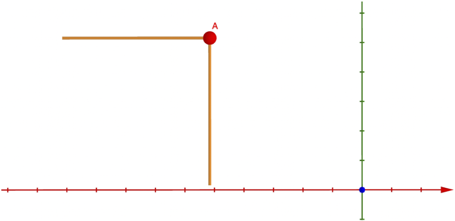
Figure 4 The corner point $A=A(\bar q)$
in the broken line
$A=A(\bar q)$
in the broken line $R_{\bar q}$
.
$R_{\bar q}$
.
The image $j(B)$
can be identified with the graph in
$j(B)$
can be identified with the graph in $\mathbb R^2\times \mathbb R^{n-1}$
of a family of broken lines
$\mathbb R^2\times \mathbb R^{n-1}$
of a family of broken lines $R_{\bar q}$
in
$R_{\bar q}$
in $\mathbb R^2$
parameterized by
$\mathbb R^2$
parameterized by $\bar q \in \mathbb R^{n-1}$
(see Figure 1 in the introduction). The image
$\bar q \in \mathbb R^{n-1}$
(see Figure 1 in the introduction). The image $j(\Delta )$
of the singular locus
$j(\Delta )$
of the singular locus $\Delta \equiv \Pi \times \{0\}$
consists of the corner points in
$\Delta \equiv \Pi \times \{0\}$
consists of the corner points in $R_{\bar q}$
for those
$R_{\bar q}$
for those $\bar q$
in the tropical hyperplane
$\bar q$
in the tropical hyperplane $\Pi $
. To sum up,
$\Pi $
. To sum up,
 $$ \begin{align} j(B)=\bigcup_{\bar q\in\mathbb R^{n-1}} R_{\bar q}\times \{\bar q\}, \, \qquad j(\Delta)=\{ (A(\bar q), \bar q) \mid \bar q\in \Pi \}. \end{align} $$
In particular, when $n=2$
, the
$n=2$
, the $j(\Delta )$
only consists of a single point (i.e., the blue point S in Figure 1).
$j(\Delta )$
only consists of a single point (i.e., the blue point S in Figure 1).
Remark 2.6. The ‘singular locus’ $j(\Delta )$
in
$j(\Delta )$
in $j(B)$
is curved just like [Reference Kontsevich and Soibelman50, p27]. Something similar is also considered in [Reference Castaño-Bernard and Matessi12, Example 3.9]. Intuitively, we start the cuts at points on a graph of a continuous function (rather than an affine one) and make the gluing in a one-dimension-higher Euclidean space.
$j(B)$
is curved just like [Reference Kontsevich and Soibelman50, p27]. Something similar is also considered in [Reference Castaño-Bernard and Matessi12, Example 3.9]. Intuitively, we start the cuts at points on a graph of a continuous function (rather than an affine one) and make the gluing in a one-dimension-higher Euclidean space.
3 B side: Kontsevich-Soibelman’s analytic fibration
In this section, we aim to develop an ‘analytic torus fibration with singularities’ on the algebraic $\Lambda $
-variety Y such that its smooth part becomes the affinoid torus fibration in the sense of [Reference Kontsevich and Soibelman50, §4.1].
$\Lambda $
-variety Y such that its smooth part becomes the affinoid torus fibration in the sense of [Reference Kontsevich and Soibelman50, §4.1].
3.1 Tropicalization map
In this paper, we exclusively consider the Novikov field $\Lambda =\mathbb C((T^{\mathbb R}))$
, a non-archimedean field that consists of all the infinite series
$\Lambda =\mathbb C((T^{\mathbb R}))$
, a non-archimedean field that consists of all the infinite series $\sum _{i=0}^\infty a_i T^{\lambda _i}$
, where
$\sum _{i=0}^\infty a_i T^{\lambda _i}$
, where $a_i\in \mathbb C$
, T is a formal symbol, and
$a_i\in \mathbb C$
, T is a formal symbol, and $\{\lambda _i\}$
is a divergent strictly-increasing sequence in
$\{\lambda _i\}$
is a divergent strictly-increasing sequence in $\mathbb R$
. It has a non-archimedean valuation
$\mathbb R$
. It has a non-archimedean valuation
 $$\begin{align*}\operatorname{\mathrm{\mathsf{v}}}: \Lambda \to \mathbb R\cup \{\infty\} \end{align*}$$
defined by sending the above series to the smallest $\lambda _i$
with
$\lambda _i$
with $a_i\neq 0$
and sending the zero series to
$a_i\neq 0$
and sending the zero series to $\infty $
. It is equivalent to the non-archimedean norm defined by
$\infty $
. It is equivalent to the non-archimedean norm defined by $|x|=\exp (-\operatorname {\mathrm {\mathsf {v}}}(x))$
. The multiplicative group is the subset
$|x|=\exp (-\operatorname {\mathrm {\mathsf {v}}}(x))$
. The multiplicative group is the subset $U_{\Lambda }=\operatorname {\mathrm {\mathsf {v}}}^{-1}(0)=\{x\in \Lambda \mid |x|=1\}$
that resembles the subgroup
$U_{\Lambda }=\operatorname {\mathrm {\mathsf {v}}}^{-1}(0)=\{x\in \Lambda \mid |x|=1\}$
that resembles the subgroup $U(1)\equiv S^1$
in
$U(1)\equiv S^1$
in $\mathbb C^*$
.
$\mathbb C^*$
.
Consider the tropicalization map
 $$ \begin{align} \operatorname{\mathrm{\mathfrak{trop}}}: (\Lambda^*)^n\to\mathbb R^n, \qquad (z_i)\mapsto (\operatorname{\mathrm{\mathsf{v}}}(z_i)). \end{align} $$
It is a continuous map with respect to the analytic topology in $(\Lambda ^*)^n$
and the Euclidean topology. Note that a fiber of
$(\Lambda ^*)^n$
and the Euclidean topology. Note that a fiber of $\operatorname {\mathrm {\mathfrak {trop}}}$
is simply a copy of
$\operatorname {\mathrm {\mathfrak {trop}}}$
is simply a copy of $U_\Lambda ^n\equiv \operatorname {\mathrm {\mathfrak {trop}}}^{-1}(0)$
up to a translation
$U_\Lambda ^n\equiv \operatorname {\mathrm {\mathfrak {trop}}}^{-1}(0)$
up to a translation $y_i\mapsto T^{c_i}y_i$
; cf. (1).
$y_i\mapsto T^{c_i}y_i$
; cf. (1).
3.2 Non-archimedean integrable system
Following Kontsevich and Soibelman [Reference Kontsevich and Soibelman50, §4], we introduce an analog of the notion of an integrable system in the non-archimedean analytic setting.
Let $\mathcal Y$
be an analytic space over
$\mathcal Y$
be an analytic space over $\Lambda $
of dimension n, and let B be an n-dimensional topological manifold or a CW complex. Let
$\Lambda $
of dimension n, and let B be an n-dimensional topological manifold or a CW complex. Let $f: \mathcal Y\to B$
a proper continuous map with respect to the analytic topology and Euclidean topology. We call a point
$f: \mathcal Y\to B$
a proper continuous map with respect to the analytic topology and Euclidean topology. We call a point $p \in B$
smooth (or f-smooth) if there is a neighborhood U of p in B such that the fibration
$p \in B$
smooth (or f-smooth) if there is a neighborhood U of p in B such that the fibration $f^{-1}(U)\to U$
is isomorphic to
$f^{-1}(U)\to U$
is isomorphic to $\operatorname {\mathrm {\mathfrak {trop}}}^{-1}(V)\to V$
for some open subset
$\operatorname {\mathrm {\mathfrak {trop}}}^{-1}(V)\to V$
for some open subset $V\subset \mathbb R^n$
. Here,
$V\subset \mathbb R^n$
. Here, $f^{-1}(U)\cong \operatorname {\mathrm {\mathfrak {trop}}}^{-1}(V)$
is an isomorphism of
$f^{-1}(U)\cong \operatorname {\mathrm {\mathfrak {trop}}}^{-1}(V)$
is an isomorphism of $\Lambda $
-analytic spaces while
$\Lambda $
-analytic spaces while $U\cong V$
is a homeomorphism.
$U\cong V$
is a homeomorphism.

Let’s call it an affinoid tropical chart, which may be also viewed as a tropical chart in the language of Chambert-Loir and Ducros [Reference Chambert-Loir and Ducros14, (3.1.2)].
Let $B_0$
denote the open subset of f-smooth points of B. We call f an
affinoid torus fibration
if
$B_0$
denote the open subset of f-smooth points of B. We call f an
affinoid torus fibration
if $B_0=B$
(see [Reference Nicaise, Xu and Yu53, §3.3]). In general, we only have
$B_0=B$
(see [Reference Nicaise, Xu and Yu53, §3.3]). In general, we only have $B_0\subsetneq B$
, but the restriction of f over
$B_0\subsetneq B$
, but the restriction of f over $B_0$
, denoted by
$B_0$
, denoted by $ f_0: f^{-1}(B_0)\to B_0, $
is always an affinoid torus fibration simply by definition.
$ f_0: f^{-1}(B_0)\to B_0, $
is always an affinoid torus fibration simply by definition.
The following construction is greatly influenced by Kontsevich-Soibelman [Reference Kontsevich and Soibelman50, §8]. But, we have to substantially generalize and modify it for our T-duality purpose in the sense of Definition 1.4. Let
 $$\begin{align*}\psi_0:\mathbb R^ {n-1} \to (0,+\infty) \end{align*}$$
be a continuous function. In practice, we choose $\psi _0(\bar q)=\psi (\bar q,0)$
to be the one in (20, 21); in this case,
$\psi _0(\bar q)=\psi (\bar q,0)$
to be the one in (20, 21); in this case, $\psi _0>0$
as the symplectic area of a holomorphic disk.
$\psi _0>0$
as the symplectic area of a holomorphic disk.
Remark 3.1. This section can be considered in the pure non-archimedean world. The constructions still hold if the Novikov field $\Lambda $
is replaced by another non-archimedean field. The existence of affinoid torus fibrations is also a central topic in non-archimedean geometry, and such research is very sparse [Reference Kontsevich and Soibelman50, Reference Nicaise, Xu and Yu53]. Now, we give a large class of
new
examples inspired by symplectic methods and SYZ picture.
$\Lambda $
is replaced by another non-archimedean field. The existence of affinoid torus fibrations is also a central topic in non-archimedean geometry, and such research is very sparse [Reference Kontsevich and Soibelman50, Reference Nicaise, Xu and Yu53]. Now, we give a large class of
new
examples inspired by symplectic methods and SYZ picture.
Recall that the $\Lambda $
-algebraic variety Y is given by the equation
$\Lambda $
-algebraic variety Y is given by the equation $ x_0 x_1=1+y_1+\cdots +y_{n-1} $
in
$ x_0 x_1=1+y_1+\cdots +y_{n-1} $
in $\Lambda ^2_{(x_0,x_1)}\times (\Lambda ^*)^{n-1}_{(y_1,\dots ,y_{n-1})}$
. As said, we will not always distinguish Y and its analytification. We define
$\Lambda ^2_{(x_0,x_1)}\times (\Lambda ^*)^{n-1}_{(y_1,\dots ,y_{n-1})}$
. As said, we will not always distinguish Y and its analytification. We define
 $$ \begin{align} F=(F_0,F_1; G_1,\dots, G_{n-1}): Y\to \mathbb R^{n+1} \end{align} $$
as follows: given $z=(x_0,x_1,y_1,\dots ,y_{n-1})$
, we set
$z=(x_0,x_1,y_1,\dots ,y_{n-1})$
, we set
 $$\begin{align*}\begin{aligned} F_0(z)&=\min\{ \operatorname{\mathrm{\mathsf{v}}}(x_0), -\psi_0(\operatorname{\mathrm{\mathsf{v}}}(y_1),\dots, \operatorname{\mathrm{\mathsf{v}}}(y_{n-1}) )+\min\{0,\operatorname{\mathrm{\mathsf{v}}}(y_1),\dots, \operatorname{\mathrm{\mathsf{v}}}(y_{n-1})\} \} \\ F_1(z)&= \min \{ \operatorname{\mathrm{\mathsf{v}}}(x_1), \ \ \ \psi_0(\operatorname{\mathrm{\mathsf{v}}}(y_1),\dots, \operatorname{\mathrm{\mathsf{v}}}(y_{n-1})) \} \\ G_k(z)&=\operatorname{\mathrm{\mathsf{v}}}(y_k) \qquad \text{for} \ 1\le k< n. \end{aligned} \end{align*}$$
This is a
tropically continuous
map in the sense of Chambert-Loir and Ducros [Reference Chambert-Loir and Ducros14, (3.1.6)]. Roughly, this means F locally takes the form $\varphi (\operatorname {\mathrm {\mathsf {v}}}(f_1),\dots , \operatorname {\mathrm {\mathsf {v}}}(f_n))$
, where
$\varphi (\operatorname {\mathrm {\mathsf {v}}}(f_1),\dots , \operatorname {\mathrm {\mathsf {v}}}(f_n))$
, where $f_i$
’s are local invertible analytic functions and
$f_i$
’s are local invertible analytic functions and $\varphi :U\to \mathbb R^m$
is a continuous map for the Euclidean topology for some open subset U of
$\varphi :U\to \mathbb R^m$
is a continuous map for the Euclidean topology for some open subset U of $\mathbb R^n$
. By adding other constraints on the
$\mathbb R^n$
. By adding other constraints on the $\varphi $
, one may define the notion of tropically piecewise-linear /
$\varphi $
, one may define the notion of tropically piecewise-linear / $C^k$
, etc.
$C^k$
, etc.
3.2.1 Description of the image of F.
Fix $\bar q=(q_1,\dots , q_{n-1})$
, and define
$\bar q=(q_1,\dots , q_{n-1})$
, and define
 $$\begin{align*}S_{\bar q}:=\{(u_0,u_1)\in\mathbb R^2\mid (u_0,u_1,\bar q)\in F(Y)\}. \end{align*}$$
In other words, the image of Y in $\mathbb R^{n+1}\equiv \mathbb R^2\times \mathbb R^{n-1}$
under F is given by
$\mathbb R^{n+1}\equiv \mathbb R^2\times \mathbb R^{n-1}$
under F is given by
 $$ \begin{align} \mathfrak B:=F(Y)=\bigcup_{\bar q\in\mathbb R^{n-1}} S_{\bar q}\times \{\bar q\}. \end{align} $$
It suffices to describe each $S_{\bar q}$
. Just like §2.1, let
$S_{\bar q}$
. Just like §2.1, let $\Pi \subset \mathbb R^{n-1}$
be the tropical hyperplane associated to
$\Pi \subset \mathbb R^{n-1}$
be the tropical hyperplane associated to $\min \{0,\bar q\}$
, consisting of those points for which
$\min \{0,\bar q\}$
, consisting of those points for which $\min \{0,\bar q\}$
is attained twice. Just as (25), we define
$\min \{0,\bar q\}$
is attained twice. Just as (25), we define
 $$ \begin{align*} a_0(\bar q)=\min\{0,\bar q\}-\psi_0(\bar q) \qquad \text{and} \qquad a_1(\bar q)=\psi_0(\bar q). \end{align*} $$
Let $z=(x_0,x_1,y_1,\dots , y_{n-1})$
be an arbitrary point in Y with
$z=(x_0,x_1,y_1,\dots , y_{n-1})$
be an arbitrary point in Y with $q_k:=\operatorname {\mathrm {\mathsf {v}}}(y_k)$
for
$q_k:=\operatorname {\mathrm {\mathsf {v}}}(y_k)$
for $1\le k<n$
. We write
$1\le k<n$
. We write $p=(u_0,u_1,\bar q)=F(z) $
for the image point.
$p=(u_0,u_1,\bar q)=F(z) $
for the image point.
-
(i) Assume
$\bar q\notin \Pi $
. Then,
$\operatorname {\mathrm {\mathsf {v}}}(x_0)+\operatorname {\mathrm {\mathsf {v}}}(x_1)=\operatorname {\mathrm {\mathsf {v}}}(1+y_1+\cdots +y_{n-1})=\min \{0,\bar q\}$
. Eliminating
$\operatorname {\mathrm {\mathsf {v}}}(x_0)$
, we get
$ F_0(z)= \min \{0,\bar q\} +\min \{-\operatorname {\mathrm {\mathsf {v}}}(x_1), -\psi _0(\bar q)\} $
and
$F_1(z)=\min \{\operatorname {\mathrm {\mathsf {v}}}(x_1), \psi _0(\bar q)\}$
. Hence, the
$S_{\bar q}$
is simply the image of the broken line in
$\mathbb R^2$
given by (30)with a corner point at
$$ \begin{align} s_{\bar q}: \mathbb R\to\mathbb R^2 , \quad c\mapsto \big( \min \{0,\bar q\}+ \min\{-c, -\psi_0(\bar q)\}, \quad \min\{c,\psi_0(\bar q)\} \big) \end{align} $$
$(a_0(\bar q), a_1(\bar q))$
. Here, c represents
$\operatorname {\mathrm {\mathsf {v}}}(x_1)$
. We take a small neighborhood
$\bar V$
of
$\bar q$
in the complement of
$\Pi $
in
$\mathbb R^{n-1}$
. Given the c with
$s_{\bar q}(c)=(u_0,u_1)$
and a sufficiently small
$\epsilon>0$
, we can find a neighborhood U of p in
$\mathfrak B$
that is homeomorphic to
$V:=(c-\epsilon , c+\epsilon )\times \bar V$
in
$\mathbb R^n$
via the various
$s_{\bar q'}$
for
$\bar q'\in \bar V$
. Then, under this identification
$U\cong V$
,
$F^{-1}(U)$
is isomorphic to
$\operatorname {\mathrm {\mathfrak {trop}}}^{-1}(V)$
by forgetting
$x_0$
(i.e.,
$z\mapsto (x_1, y_1,\dots , y_{n-1})$
). In this way, the fibration F also agrees with
$\operatorname {\mathrm {\mathfrak {trop}}}$
. In conclusion, this means p is an F-smooth point in the sense of §3.2.
-
(ii) Assume
$\bar q\in \Pi $
. Recall
$F_0(z)=\min \{ \operatorname {\mathrm {\mathsf {v}}}(x_0), a_0(\bar q)\}$
and
$F_1(z)=\min \{\operatorname {\mathrm {\mathsf {v}}}(x_1),a_1(\bar q)\}$
. As
$\operatorname {\mathrm {\mathsf {v}}}(x_0)+\operatorname {\mathrm {\mathsf {v}}}(x_1)\ge \min \{\operatorname {\mathrm {\mathsf {v}}}(1),\operatorname {\mathrm {\mathsf {v}}}(y_1),\dots ,\operatorname {\mathrm {\mathsf {v}}}(y_{n-1})\}=a_0(\bar q)+a_1(\bar q)$
, one of the following cases must hold:-
(ii-a) If
$\operatorname {\mathrm {\mathsf {v}}}(x_0)<a_0(\bar q)$
, then
$\operatorname {\mathrm {\mathsf {v}}}(x_1)>a_1(\bar q)$
. Hence,
$F_0(z)=\operatorname {\mathrm {\mathsf {v}}}(x_0) \equiv u_0$
, and
$F_1(z)=a_1(\bar q)$
. Find a neighborhood U of p in
$\mathfrak B$
in the form
$U=\{(u_0', a_1(\bar q'), \bar q') \mid u_0' \in I, \bar q'\in \bar V\}$
, where a neighborhood
$\bar V$
of
$\bar q$
and an open interval I centered at
$u_0$
are both chosen small enough so that
$u_0'<a_0(\bar q')$
always holds. Let
$V:=I\times \bar V \cong U$
, and
$F^{-1}(U)$
is isomorphic to
$\operatorname {\mathrm {\mathfrak {trop}}}^{-1}(V)$
by forgetting
$x_1$
. Therefore, p is F-smooth. -
(ii-b) If
$\operatorname {\mathrm {\mathsf {v}}}(x_1) < a_1(\bar q)$
, then
$\operatorname {\mathrm {\mathsf {v}}}(x_0)>a_0(\bar q)$
. Hence,
$F_0(z)= a_0(\bar q)$
, and
$F_1(z)=\operatorname {\mathrm {\mathsf {v}}}(x_1) \equiv u_1$
. In a similar way, we can show p is also F-smooth. -
(ii-c) If both
$\mathsf v(x_0)\ge a_0(\bar q)$
and
$\mathsf v(x_1)\ge a_1(\bar q)$
, then
$(u_0,u_1)=(F_0(z),F_1(z))=(a_0(\bar q), a_1(\bar q))$
is exactly the corner point of the broken line
$s_{\bar q}$
in (30). One can also check p is not F-smooth.
Hence, the
$S_{\bar q}$
is still given by the broken line
$s_{\bar q}$
defined in the same way as (30). Moreover, by (ii-a) and (ii-b), the set of F-smooth points in
$S_{\bar q}\cong S_{\bar q}\times \{\bar q\}$
includes the union of
$ S_{\bar q}^+:= (-\infty , a_0(\bar q)) \times \{a_1(\bar q)\} $
and
$ S_{\bar q}^-:=\{a_0(\bar q)\} \times (-\infty , a_1(\bar q)) $
. -


Combining (i) and (ii) above, we have proved the following structural result:
Theorem 3.2. The map F restricts to an affinoid torus fibration over $\mathfrak B_0 \equiv \mathfrak B\setminus \hat \Delta $
, where
$\mathfrak B_0 \equiv \mathfrak B\setminus \hat \Delta $
, where
 $$\begin{align*}\hat \Delta := \bigsqcup_{\bar q\in \Pi} \{ \big(a_0(\bar q), a_1(\bar q)\big)\} \times \{\bar q\}. \end{align*}$$
3.3 Definition of f
Notice that if ![]() is a topological embedding, then
is a topological embedding, then $\jmath ^{-1} \circ F$
is also an affinoid torus fibration on its domain, by definition (§3.2). For the base
$\jmath ^{-1} \circ F$
is also an affinoid torus fibration on its domain, by definition (§3.2). For the base $B\equiv \mathbb R^n$
in §2.1 and the
$B\equiv \mathbb R^n$
in §2.1 and the $j:B\to \mathbb R^{n+1}$
in §2.4, a comparison between §2.4.2 and §3.2.1 implies the following
$j:B\to \mathbb R^{n+1}$
in §2.4, a comparison between §2.4.2 and §3.2.1 implies the following
Lemma 3.3. $j(B)$
agrees with the open subset
$j(B)$
agrees with the open subset
 $$ \begin{align} \hat B:=\{ (u_0,u_1, \bar q)\in \mathfrak B \mid u_1>0\} \subset \mathbb R^{n+1}. \end{align} $$
Moreover, we have $j(\Delta )=\hat \Delta $
. In particular,
$j(\Delta )=\hat \Delta $
. In particular, $B=j^{-1}(\hat B)$
and
$B=j^{-1}(\hat B)$
and $B_0=j^{-1}(\hat B \setminus \hat \Delta )$
.
$B_0=j^{-1}(\hat B \setminus \hat \Delta )$
.
Proof. It suffices to compare the $\bar q$
-slices for any fixed
$\bar q$
-slices for any fixed $\bar q\in \mathbb R^{n-1}$
. First, let’s indicate the coincidence between the
$\bar q\in \mathbb R^{n-1}$
. First, let’s indicate the coincidence between the $r_{\bar q}$
in (24) and the
$r_{\bar q}$
in (24) and the $s_{\bar q}$
in (30). The only difference is the domains are
$s_{\bar q}$
in (30). The only difference is the domains are $(0,+\infty )$
and
$(0,+\infty )$
and $\mathbb R$
, respectively, and
$\mathbb R$
, respectively, and $R_{\bar q}=\{(u_0,u_1)\in S_{\bar q}\mid u_1>0\}$
. Finally, using (26) and (29) completes the proof.
$R_{\bar q}=\{(u_0,u_1)\in S_{\bar q}\mid u_1>0\}$
. Finally, using (26) and (29) completes the proof.
Define $ \mathscr Y :=F^{-1}(\hat B) $
, and it is exactly given by
$ \mathscr Y :=F^{-1}(\hat B) $
, and it is exactly given by $\operatorname {\mathrm {\mathsf {v}}}(x_1)>0$
or, equivalently,
$\operatorname {\mathrm {\mathsf {v}}}(x_1)>0$
or, equivalently, $|x_1|<1$
. In particular,
$|x_1|<1$
. In particular, $j(B)=F(\mathscr Y)$
. Using the topological embedding j in (22), we define
$j(B)=F(\mathscr Y)$
. Using the topological embedding j in (22), we define $f:= j^{-1}\circ F|_{\mathscr Y}$
. By Theorem 3.2,
$f:= j^{-1}\circ F|_{\mathscr Y}$
. By Theorem 3.2, $f_0:=f|_{B_0}$
is an affinoid torus fibration. We set
$f_0:=f|_{B_0}$
is an affinoid torus fibration. We set $\mathscr Y_0:=f_0^{-1}(B_0)$
. It is not hard to show
$\mathscr Y_0:=f_0^{-1}(B_0)$
. It is not hard to show $\mathscr Y_0$
is Zariski dense in Y (e.g., by dimension reasons; compare also [Reference Payne55]). Notably, our construction of f here is purely non-archimedean and does not use any Floer theory so far.
$\mathscr Y_0$
is Zariski dense in Y (e.g., by dimension reasons; compare also [Reference Payne55]). Notably, our construction of f here is purely non-archimedean and does not use any Floer theory so far.

4 Family Floer mirror construction: an easy-to-use review
One may first skip §4 for the mere affine geometry matching in §1.3 (see a reader guide in Remark 5.3). For the legibility, we plan to substantially simplify the exposition of the mirror construction in [Reference Yuan61] in an easy-to-use way. These costs we pay are briefly explained in Remark 4.2, 4.3, 4.5 for serious readers.
4.1 Statement
Let $(X,\omega , J)$
be a Kähler manifold of real dimension
$(X,\omega , J)$
be a Kähler manifold of real dimension $2n$
. Suppose there is a Lagrangian torus fibration
$2n$
. Suppose there is a Lagrangian torus fibration $\pi _0:X_0 \to B_0$
on some open domain
$\pi _0:X_0 \to B_0$
on some open domain $X_0\subset X$
; we require it is semipositive in the sense that there is no holomorphic stable disk of negative Maslov index bounding a Lagrangian fiber. By [Reference Auroux5, Lemma 3.1], every special Lagrangian (or graded Lagrangian) satisfies this condition. Further, we require that all Lagrangian fibers are weakly unobstructed (see, for example, [Reference Auroux6, Page 7]) in the sense that their associated minimal model
$X_0\subset X$
; we require it is semipositive in the sense that there is no holomorphic stable disk of negative Maslov index bounding a Lagrangian fiber. By [Reference Auroux5, Lemma 3.1], every special Lagrangian (or graded Lagrangian) satisfies this condition. Further, we require that all Lagrangian fibers are weakly unobstructed (see, for example, [Reference Auroux6, Page 7]) in the sense that their associated minimal model $A_\infty $
algebras have vanishing obstruction ideal (slightly different from the Maurer-Cartan equations in the literature). Thanks to Solomon [Reference Solomon57], a nice sufficient condition is when each Lagrangian fiber is preserved by an anti-symplectic involution
$A_\infty $
algebras have vanishing obstruction ideal (slightly different from the Maurer-Cartan equations in the literature). Thanks to Solomon [Reference Solomon57], a nice sufficient condition is when each Lagrangian fiber is preserved by an anti-symplectic involution $\varphi $
(see also [Reference Castaño-Bernard, Matessi and Solomon13]). For example, the Gross Lagrangian fibration in §2.1 or in (2) admits the involution given by the complex conjugations
$\varphi $
(see also [Reference Castaño-Bernard, Matessi and Solomon13]). For example, the Gross Lagrangian fibration in §2.1 or in (2) admits the involution given by the complex conjugations $z_i\mapsto \bar z_i$
. In general, such an involution
$z_i\mapsto \bar z_i$
. In general, such an involution $\varphi $
gives a pairing on
$\varphi $
gives a pairing on $\pi _2(X, L_q)$
via
$\pi _2(X, L_q)$
via $\beta \leftrightarrow -\varphi _*\beta $
, inducing a pairwise canceling for the obstruction formal power series. Beware that it does not mean the virtual counts of Maslov-0 disks vanish, and they do still contribute to the homological perturbations for the minimal model
$\beta \leftrightarrow -\varphi _*\beta $
, inducing a pairwise canceling for the obstruction formal power series. Beware that it does not mean the virtual counts of Maslov-0 disks vanish, and they do still contribute to the homological perturbations for the minimal model $A_\infty $
algebras and the wall-crossing
$A_\infty $
algebras and the wall-crossing $A_\infty $
homotopy equivalence.
$A_\infty $
homotopy equivalence.
Now, the family Floer mirror construction in [Reference Yuan61] can be stated as follows:
Theorem 4.1. Given $(X,\pi _0)$
as above, there is a triple
$(X,\pi _0)$
as above, there is a triple $(X_0^\vee ,W_0^\vee , \pi _0^\vee )$
consisting of a non-archimedean analytic space
$(X_0^\vee ,W_0^\vee , \pi _0^\vee )$
consisting of a non-archimedean analytic space $X_0^\vee $
over
$X_0^\vee $
over $\Lambda $
, a global analytic function
$\Lambda $
, a global analytic function $W_0^\vee $
, and a dual affinoid torus fibration
$W_0^\vee $
, and a dual affinoid torus fibration ${\pi _0^\vee : X_0^\vee \to B_0}$
such that
${\pi _0^\vee : X_0^\vee \to B_0}$
such that
-
1. The non-archimedean analytic structure of
$(X_0^\vee , W_0^\vee , \pi _0^\vee )$
is unique up to isomorphism. -
2. The integral affine structure on
$B_0$
induced by
$\pi _0^\vee $
coincides with the one induced by
$\pi _0$
. -
3. The set of closed points in
$X_0^\vee $
coincides with (33)where
$$ \begin{align} \textstyle \bigcup_{q\in B_0} H^1(L_q; U_\Lambda), \end{align} $$
$U_\Lambda $
is the unit circle in the Novikov field
$\Lambda $
.


Beware that the mere homotopy invariance of Maurer-Cartan sets is quite insufficient to develop the analytic topology on $X_0^\vee $
for which we must seek more structure and information. In our specific SYZ context, the Maurer-Cartan sets are simply
$X_0^\vee $
for which we must seek more structure and information. In our specific SYZ context, the Maurer-Cartan sets are simply $H^1(L_q;\Lambda _0)$
, which can at most give certain set-theoretic or local approximation. This is one key point missing in [Reference Tu59]; see Remark 4.2, 4.3 for more discussions. Indeed, the new ud-homotopy theory in [Reference Yuan61] is necessary to upgrade the conventional Maurer-Cartan picture to a higher level, matching adic-convergent formal power series instead of just bijection of sets. The virtual counts of Maslov-0 disks lead to an analytic space structure on the above fiber-wise union (33) of the space of
$H^1(L_q;\Lambda _0)$
, which can at most give certain set-theoretic or local approximation. This is one key point missing in [Reference Tu59]; see Remark 4.2, 4.3 for more discussions. Indeed, the new ud-homotopy theory in [Reference Yuan61] is necessary to upgrade the conventional Maurer-Cartan picture to a higher level, matching adic-convergent formal power series instead of just bijection of sets. The virtual counts of Maslov-0 disks lead to an analytic space structure on the above fiber-wise union (33) of the space of $U_\Lambda $
-local systems. Moreover, the counts of Maslov-2 disks give rise to the global potential function
$U_\Lambda $
-local systems. Moreover, the counts of Maslov-2 disks give rise to the global potential function $W_0^\vee $
on
$W_0^\vee $
on $X_0^\vee $
.
$X_0^\vee $
.
4.2 Local affinoid tropical charts
Let $U\subset B_0$
be a contractible open subset, and choose a point
$U\subset B_0$
be a contractible open subset, and choose a point $q_0$
near U (
$q_0$
near U ( $q_0\notin U$
is possible). We require U is sufficiently small and
$q_0\notin U$
is possible). We require U is sufficiently small and $q_0$
is sufficiently close to U so that the reverse isoperimetric inequalities hold uniformly over a neighborhood of
$q_0$
is sufficiently close to U so that the reverse isoperimetric inequalities hold uniformly over a neighborhood of $U\cup \{q_0\}$
. Let
$U\cup \{q_0\}$
. Let
 $$\begin{align*}\chi: (U,q_0) \xrightarrow{\cong} (V,c)\subset \mathbb R^n \end{align*}$$
be a (pointed) integral affine coordinate chart such that $\chi (q_0)=c$
. Then, we have an identification
$\chi (q_0)=c$
. Then, we have an identification
 $$ \begin{align} \tau: (\pi_0^\vee)^{-1}(U) \xrightarrow{\cong} \operatorname{\mathrm{\mathfrak{trop}}}^{-1}(V-c) \end{align} $$
with $\operatorname {\mathrm {\mathfrak {trop}}}\circ \ \tau =\chi \circ \pi _0^\vee $
. Let’s call
$\operatorname {\mathrm {\mathfrak {trop}}}\circ \ \tau =\chi \circ \pi _0^\vee $
. Let’s call $\tau $
a (pointed) affinoid tropical chart as in §3.2. Recall that the left side is the disjoint union
$\tau $
a (pointed) affinoid tropical chart as in §3.2. Recall that the left side is the disjoint union $(\pi _0^\vee )^{-1}(U)\equiv \bigcup _{q\in U} H^1(L_q; U_\Lambda )$
set-theoretically. A closed point
$(\pi _0^\vee )^{-1}(U)\equiv \bigcup _{q\in U} H^1(L_q; U_\Lambda )$
set-theoretically. A closed point $ \mathbf y$
in the dual fiber
$ \mathbf y$
in the dual fiber $H^1(L_q; U_\Lambda )$
can be viewed as a group homomorphism
$H^1(L_q; U_\Lambda )$
can be viewed as a group homomorphism $\pi _1(L_q)\to U_\Lambda $
(i.e., a flat
$\pi _1(L_q)\to U_\Lambda $
(i.e., a flat $U_\Lambda $
-connection modulo gauge equivalence), and we have the natural pairing
$U_\Lambda $
-connection modulo gauge equivalence), and we have the natural pairing
 $$ \begin{align} \pi_1(L_q)\times H^1(L_q; U_\Lambda)\to U_\Lambda, \qquad (\alpha, \mathbf y) \mapsto \mathbf y^\alpha. \end{align} $$
Write $\chi =(\chi _1,\dots , \chi _n)$
, and it gives rise to a continuous family
$\chi =(\chi _1,\dots , \chi _n)$
, and it gives rise to a continuous family $e_i=e_i(q)$
of
$e_i=e_i(q)$
of $\mathbb Z$
-bases of
$\mathbb Z$
-bases of $\pi _1(L_q)$
for all
$\pi _1(L_q)$
for all $q\in U$
, cf. (12). Then, the corresponding affinoid tropical chart
$q\in U$
, cf. (12). Then, the corresponding affinoid tropical chart $\tau $
has a very concrete description:
$\tau $
has a very concrete description:
 $$ \begin{align} \tau(\mathbf y)= (T^{\chi_1(q)} \mathbf y^{e_1(q)},\dots, T^{\chi_n(q)} \mathbf y^{e_n(q)} ). \end{align} $$
Remark 4.2. The above picture is oversimplified. To develop the analytic topology, we must study local affinoid spaces or equivalently the corresponding affinoid algebras. Specifically, in the above (34), we may first assume $V=\chi (U)$
is a rational polytope in
$V=\chi (U)$
is a rational polytope in $\mathbb R^n$
. Given a base point
$\mathbb R^n$
. Given a base point $q_0$
, any
$q_0$
, any $q\in U$
can be viewed as a vector, denoted by
$q\in U$
can be viewed as a vector, denoted by $q-q_0$
, in
$q-q_0$
, in $H^1(L_{q_0}; \mathbb R)\cong T_{q_0} B$
. Instead of (34), we should more precisely identify
$H^1(L_{q_0}; \mathbb R)\cong T_{q_0} B$
. Instead of (34), we should more precisely identify $(\pi _0^\vee )^{-1}(U)$
with the maximal ideal spectrum (or the multiplicative seminorm spectrum) of the polyhedral affinoid algebra
$(\pi _0^\vee )^{-1}(U)$
with the maximal ideal spectrum (or the multiplicative seminorm spectrum) of the polyhedral affinoid algebra $\Lambda \langle U, q_0 \rangle $
[Reference Einsiedler, Kapranov and Lind26]. It consists of the Laurent formal power series inside
$\Lambda \langle U, q_0 \rangle $
[Reference Einsiedler, Kapranov and Lind26]. It consists of the Laurent formal power series inside $\Lambda [[\pi _1(L_{q_0})]]$
that have the form
$\Lambda [[\pi _1(L_{q_0})]]$
that have the form $\sum _{\alpha \in \pi _1(L_{q_0})} c_\alpha Y^\alpha $
with
$\sum _{\alpha \in \pi _1(L_{q_0})} c_\alpha Y^\alpha $
with $c_\alpha \in \Lambda $
and
$c_\alpha \in \Lambda $
and $\operatorname {\mathrm {\mathsf {v}}}(c_\alpha )+\langle \alpha , q-q_0 \rangle \to \infty $
as
$\operatorname {\mathrm {\mathsf {v}}}(c_\alpha )+\langle \alpha , q-q_0 \rangle \to \infty $
as $|\alpha |\to \infty $
for any
$|\alpha |\to \infty $
for any $q \in U$
. Here, Y is a symbol and
$q \in U$
. Here, Y is a symbol and $Y^\alpha $
are the monomials. Now, a closed point
$Y^\alpha $
are the monomials. Now, a closed point $\mathbf y\in H^1(L_{q}; U_\Lambda )$
for some
$\mathbf y\in H^1(L_{q}; U_\Lambda )$
for some $q\in U$
corresponds to the maximal ideal in
$q\in U$
corresponds to the maximal ideal in $\Lambda \langle U, q_0\rangle $
generated by
$\Lambda \langle U, q_0\rangle $
generated by $Y^\alpha - T^{\langle \alpha , q-q_0\rangle }\mathbf y^{\alpha (q)}$
for all
$Y^\alpha - T^{\langle \alpha , q-q_0\rangle }\mathbf y^{\alpha (q)}$
for all $\alpha \in \pi _1(L_{q_0})$
, where
$\alpha \in \pi _1(L_{q_0})$
, where $\alpha (q)\in \pi _1(L_q)$
denotes the induced class; cf. (12). Finally, we must choose U to be sufficiently small, subject to Groman-Solomon’s reverse isoperimetric inequality [Reference Evans28, Reference Groman and Solomon38] for the non-archimedean convergence. We also need to generalize it to a uniform version as in [Reference Yuan61]; otherwise, as this inequality depends on the base point, we cannot ensure the convergence for the analytic gluing (cf. Remark 4.3).
$\alpha (q)\in \pi _1(L_q)$
denotes the induced class; cf. (12). Finally, we must choose U to be sufficiently small, subject to Groman-Solomon’s reverse isoperimetric inequality [Reference Evans28, Reference Groman and Solomon38] for the non-archimedean convergence. We also need to generalize it to a uniform version as in [Reference Yuan61]; otherwise, as this inequality depends on the base point, we cannot ensure the convergence for the analytic gluing (cf. Remark 4.3).
4.3 Gluing
In the construction of Theorem 4.1, we start with various local affinoid tropical charts as above, and then we can develop transition maps (or call gluing maps) among them in a choice-independent manner. This process encodes the quantum corrections of the pseudo-holomorphic disks bounded by smooth $\pi $
-fibers but possibly meeting the singular
$\pi $
-fibers but possibly meeting the singular $\pi $
-fibers (Red disks in Figure 2).
$\pi $
-fibers (Red disks in Figure 2).
Let’s take two pointed integral affine charts. Replacing the two domains by their intersection, we may assume the two charts have the same domain $U\subset B_0$
, but the base points may be different and outside of U. Namely, as before in Section 4.2, we take two pointed integral affine charts
$U\subset B_0$
, but the base points may be different and outside of U. Namely, as before in Section 4.2, we take two pointed integral affine charts
 $$\begin{align*}\chi_a=(\chi_{a1},\dots, \chi_{an}):(U,q_a) \to (V_a,c_a) \end{align*}$$
for $a=1,2$
. Then,
$a=1,2$
. Then, $\unicode{x3c7} :=\chi _2\circ \chi _1^{-1}:V_1\to V_2$
is an integral affine transformation. Due to (34) above, we have two affinoid tropical charts on the same domain:
$\unicode{x3c7} :=\chi _2\circ \chi _1^{-1}:V_1\to V_2$
is an integral affine transformation. Due to (34) above, we have two affinoid tropical charts on the same domain:
 $$\begin{align*}\tau_a: (\pi_0^\vee)^{-1}(U)\to \operatorname{\mathrm{\mathfrak{trop}}}^{-1}(V_a-c_a) \end{align*}$$
such that $\chi _a\circ \pi _0^\vee =\operatorname {\mathrm {\mathfrak {trop}}}\circ \ \tau _a$
for
$\chi _a\circ \pi _0^\vee =\operatorname {\mathrm {\mathfrak {trop}}}\circ \ \tau _a$
for $a=1,2$
.
$a=1,2$
.
The transition map between the two charts $\tau _1$
and
$\tau _1$
and $\tau _2$
is an automorphism map
$\tau _2$
is an automorphism map $\phi $
that, concerning the Fukaya’s trick, captures the wall-crossing information of a Lagrangian isotopy from
$\phi $
that, concerning the Fukaya’s trick, captures the wall-crossing information of a Lagrangian isotopy from $L_{q_1}$
to
$L_{q_1}$
to $L_{q_2}$
. In brief, we can view it as a fiber-preserving map:
$L_{q_2}$
. In brief, we can view it as a fiber-preserving map:
 $$ \begin{align} \phi: \bigcup_{q\in U} H^1(L_q; U_\Lambda)\to \bigcup_{q\in U} H^1(L_q;U_\Lambda). \end{align} $$
But, be careful. The source and the target of $\phi $
should correspond to the two different affinoid tropical charts
$\phi $
should correspond to the two different affinoid tropical charts $\tau _1$
and
$\tau _1$
and $\tau _2$
, respectively, although they are set-theoretically the same. In particular, the base points
$\tau _2$
, respectively, although they are set-theoretically the same. In particular, the base points $q_a$
for
$q_a$
for $\tau _a$
matter a lot for the analytic structure. Indeed, by the two affinoid tropical charts
$\tau _a$
matter a lot for the analytic structure. Indeed, by the two affinoid tropical charts $\tau _1$
and
$\tau _1$
and $\tau _2$
, the gluing map
$\tau _2$
, the gluing map $\phi $
can be regarded an analytic map between open subdomains in
$\phi $
can be regarded an analytic map between open subdomains in $(\Lambda ^*)^n$
as follows:
$(\Lambda ^*)^n$
as follows:
 $$ \begin{align} \Phi:= \tau_2\circ \phi \circ \tau_1^{-1}: \operatorname{\mathrm{\mathfrak{trop}}}^{-1}(V_1-c_1)\to \operatorname{\mathrm{\mathfrak{trop}}}^{-1}(V_2-c_2). \end{align} $$
By definition, if $\mathbf y $
is a point in
$\mathbf y $
is a point in $ H^1(L_q; U_\Lambda )$
for some
$ H^1(L_q; U_\Lambda )$
for some $q\in U$
, then
$q\in U$
, then $\tilde { \mathbf y} :=\phi (\mathbf y)$
is a point in the same fiber
$\tilde { \mathbf y} :=\phi (\mathbf y)$
is a point in the same fiber $H^1(L_q;U_\Lambda )$
and is subject to the following condition:
$H^1(L_q;U_\Lambda )$
and is subject to the following condition:
 $$ \begin{align} \tilde{\mathbf y}^\alpha= \mathbf y^\alpha \exp \langle \alpha, \pmb {\mathfrak{F}}(\mathbf y) \rangle, \end{align} $$
where we use the pairing in (35) and $\pmb {\mathfrak {F}}$
is a vector-valued formal power seriesFootnote
1
in
$\pmb {\mathfrak {F}}$
is a vector-valued formal power seriesFootnote
1
in $ \Lambda [[\pi _1(L_{q})]]\hat \otimes H^1(L_{q})$
. Roughly, the
$ \Lambda [[\pi _1(L_{q})]]\hat \otimes H^1(L_{q})$
. Roughly, the $\pmb {\mathfrak {F}}$
is decided by the virtual counts of Maslov-0 disksFootnote
2
along a Lagrangian isotopy from
$\pmb {\mathfrak {F}}$
is decided by the virtual counts of Maslov-0 disksFootnote
2
along a Lagrangian isotopy from $L_{q_1}$
to
$L_{q_1}$
to $L_{q_2}$
. The existence and uniqueness of such a
$L_{q_2}$
. The existence and uniqueness of such a $\pmb {\mathfrak {F}}$
is proved in [Reference Yuan61]. By definition, the Novikov coefficients of
$\pmb {\mathfrak {F}}$
is proved in [Reference Yuan61]. By definition, the Novikov coefficients of $\pmb {\mathfrak {F}}$
have positive valuations, and one can prove the
$\pmb {\mathfrak {F}}$
have positive valuations, and one can prove the $\exp \langle \alpha , \pmb {\mathfrak {F}}\rangle $
has valuation zero for sufficiently small U by the reverse isoperimetric inequality again. In particular,
$\exp \langle \alpha , \pmb {\mathfrak {F}}\rangle $
has valuation zero for sufficiently small U by the reverse isoperimetric inequality again. In particular, $\phi $
preserves the fibers.
$\phi $
preserves the fibers.
Remark 4.3. Again, we must work with the category of affinoid algebras to be completely rigorous. The gluing map $\phi \equiv \psi ^*$
comes from an affinoid algebra homomorphism:
$\phi \equiv \psi ^*$
comes from an affinoid algebra homomorphism:
 $$ \begin{align} \psi: \Lambda \langle U, q_2\rangle \to \Lambda\langle U, q_1\rangle, \qquad Y^{\alpha(q_2)} \mapsto T^{\langle \alpha, q_1-q_2\rangle} Y^{\alpha(q_1)} \exp\langle \alpha, \pmb {\mathfrak{F}}(Y)\rangle \end{align} $$
for
 $$ \begin{align} \pmb {\mathfrak{F}}=\sum_{\mu(\beta)=0} T^{E(\beta)} Y^{\partial\beta} \mathfrak f_{0,\beta}, \end{align} $$
where $\mathfrak f=\{\mathfrak f_{k,\beta }\} \ (k\ge 0, \beta \in \pi _2(X,L_q))$
is, up to Fukaya’s trick, some
$\mathfrak f=\{\mathfrak f_{k,\beta }\} \ (k\ge 0, \beta \in \pi _2(X,L_q))$
is, up to Fukaya’s trick, some $A_\infty $
(ud-)homotopy equivalence between two
$A_\infty $
(ud-)homotopy equivalence between two $A_\infty $
algebras associated to
$A_\infty $
algebras associated to $L_{q_1}$
and
$L_{q_1}$
and $L_{q_2}$
. We can finally check that the simplified description (39) agrees with (40) using the perspective of Remark 4.2.
$L_{q_2}$
. We can finally check that the simplified description (39) agrees with (40) using the perspective of Remark 4.2.
The idea of finding (40) is to use the coordinate change in [Reference Fukaya33, (1.6)] to the morphism [Reference Fukaya, Oh, Ohta and Ono35, (3.6.37)], and it is first discovered by J. Tu in [Reference Tu59]. But, we cannot just naively use the homotopy invariance of Maurer-Cartan sets to get the analytic topology on $X_0^\vee $
. Indeed, the idea of Maurer-Cartan invariance is overall correct but needs to be carried out in a more precise level, matching adic-convergent formal power series rather than just bijections of sets. For this, we need the stronger ud-homotopy in [Reference Yuan61]; we also need a uniform version of reverse isoperimetric inequality (cf. Remark 4.2) for the non-archimedean convergence issues when we move between adjacent local tropical charts.
$X_0^\vee $
. Indeed, the idea of Maurer-Cartan invariance is overall correct but needs to be carried out in a more precise level, matching adic-convergent formal power series rather than just bijections of sets. For this, we need the stronger ud-homotopy in [Reference Yuan61]; we also need a uniform version of reverse isoperimetric inequality (cf. Remark 4.2) for the non-archimedean convergence issues when we move between adjacent local tropical charts.
Finally, note that the $A_\infty $
morphism
$A_\infty $
morphism $\mathfrak f$
is obtained by a parameterized moduli space of holomorphic disks and is highly choice-sensitive. But surprisingly, the gluing map
$\mathfrak f$
is obtained by a parameterized moduli space of holomorphic disks and is highly choice-sensitive. But surprisingly, the gluing map $\phi $
is actually unchanged for any such
$\phi $
is actually unchanged for any such $A_\infty $
(ud-)homotopy equivalence. This is missed in [Reference Tu59] but is proved in [Reference Yuan61] by the ud-homotopy relations. In our opinion, the choice-independence of the gluing maps is the cornerstone of everything about the family Floer mirror construction, including the results in this paper as well as those in [Reference Yuan63] [Reference Yuan62].
$A_\infty $
(ud-)homotopy equivalence. This is missed in [Reference Tu59] but is proved in [Reference Yuan61] by the ud-homotopy relations. In our opinion, the choice-independence of the gluing maps is the cornerstone of everything about the family Floer mirror construction, including the results in this paper as well as those in [Reference Yuan63] [Reference Yuan62].
4.4 Void wall-crossing
Let $B_1\subset B_0$
be a contractible open set. Let
$B_1\subset B_0$
be a contractible open set. Let $B_2=\{x\in B_0\mid \operatorname {\mathrm {dist}} (x, B_1) < \epsilon \}$
be a slight thickening of
$B_2=\{x\in B_0\mid \operatorname {\mathrm {dist}} (x, B_1) < \epsilon \}$
be a slight thickening of $B_1$
in
$B_1$
in $B_0$
. We assume it is also contractible and
$B_0$
. We assume it is also contractible and $\epsilon>0$
is a sufficiently small number so that the estimate constant in the reverse isoperimetric inequalities for any Lagrangian fiber over
$\epsilon>0$
is a sufficiently small number so that the estimate constant in the reverse isoperimetric inequalities for any Lagrangian fiber over $B_1$
exceeds
$B_1$
exceeds $\epsilon $
uniformly (cf. Remark 4.2, 4.3, and [Reference Yuan61]). Then, we have the following:
$\epsilon $
uniformly (cf. Remark 4.2, 4.3, and [Reference Yuan61]). Then, we have the following:
Proposition 4.4. Let ![]() be an integral affine coordinate chart. If for every
be an integral affine coordinate chart. If for every $q\in B_1$
, the Lagrangian fiber
$q\in B_1$
, the Lagrangian fiber $L_{q}$
bounds no non-constant Maslov index zero holomorphic disk, then there is an affinoid tropical chart
$L_{q}$
bounds no non-constant Maslov index zero holomorphic disk, then there is an affinoid tropical chart $(\pi _0^\vee )^{-1} (B_2) \cong \operatorname {\mathrm {\mathfrak {trop}}}^{-1}(\chi (B_2))$
.
$(\pi _0^\vee )^{-1} (B_2) \cong \operatorname {\mathrm {\mathfrak {trop}}}^{-1}(\chi (B_2))$
.
Proof. First, since $B_2$
is contractible, we can first single out a fixed pointed integral affine chart
$B_2$
is contractible, we can first single out a fixed pointed integral affine chart $\chi : (B_2, q_0) \to (V, c) \subset \mathbb R^n$
for some point
$\chi : (B_2, q_0) \to (V, c) \subset \mathbb R^n$
for some point $q_0\in B_2$
. Next, we can cover
$q_0\in B_2$
. Next, we can cover $B_2$
by pointed integral affine coordinate charts
$B_2$
by pointed integral affine coordinate charts $\chi _i: (U_i, q_i) \to (V_i, v_i)$
,
$\chi _i: (U_i, q_i) \to (V_i, v_i)$
, $ i\in \mathcal I$
. We may require
$ i\in \mathcal I$
. We may require $\chi _i=\chi |_{U_i}$
and the diameters of
$\chi _i=\chi |_{U_i}$
and the diameters of $U_i$
are less than
$U_i$
are less than $\epsilon $
. In particular, we may require all
$\epsilon $
. In particular, we may require all $q_i$
’s are contained in
$q_i$
’s are contained in $B_1$
, and there will be no Maslov-0 disks along a Lagrangian isotopy among the fibers between any pair of
$B_1$
, and there will be no Maslov-0 disks along a Lagrangian isotopy among the fibers between any pair of $q_i$
’s inside
$q_i$
’s inside $B_1$
. However, just like (34), we have many affinoid tropical charts
$B_1$
. However, just like (34), we have many affinoid tropical charts $\tau _i: (\pi _0^\vee )^{-1}(U_i)\cong \operatorname {\mathrm {\mathfrak {trop}}}^{-1}( V_i-v_i)$
. The gluing maps among these tropical charts take the form as in (38). However, due to the non-existence of the Maslov-0 holomorphic disks, they have no twisting terms and take the simplest form
$\tau _i: (\pi _0^\vee )^{-1}(U_i)\cong \operatorname {\mathrm {\mathfrak {trop}}}^{-1}( V_i-v_i)$
. The gluing maps among these tropical charts take the form as in (38). However, due to the non-existence of the Maslov-0 holomorphic disks, they have no twisting terms and take the simplest form $y_i\mapsto T^{c_i} y_i$
. In conclusion, we can get a single affinoid tropical chart by gluing all these
$y_i\mapsto T^{c_i} y_i$
. In conclusion, we can get a single affinoid tropical chart by gluing all these $\tau _i$
’s.
$\tau _i$
’s.
4.5 Superpotential
Assume $\beta \in \pi _2(X,L_{q_0})$
has Maslov index two (i.e.,
$\beta \in \pi _2(X,L_{q_0})$
has Maslov index two (i.e., $\mu (\beta )=2$
, and it also induces
$\mu (\beta )=2$
, and it also induces $\beta \equiv \beta (q)\in \pi _1(L_q)$
for any q in a small contractible neighborhood of
$\beta \equiv \beta (q)\in \pi _1(L_q)$
for any q in a small contractible neighborhood of $q_0$
in
$q_0$
in $B_0$
). Denote by
$B_0$
). Denote by $\mathsf n_\beta \equiv \mathsf n_{\beta (q)}$
the corresponding open Gromov-Witten invariant.Footnote
3
It depends on the base point q and the almost complex structure J in use. For our purpose, unless the Fukaya’s trick is applied, we always use the same J in this paper. Then, due to the wall-crossing phenomenon, one may roughly think the numbers
$\mathsf n_\beta \equiv \mathsf n_{\beta (q)}$
the corresponding open Gromov-Witten invariant.Footnote
3
It depends on the base point q and the almost complex structure J in use. For our purpose, unless the Fukaya’s trick is applied, we always use the same J in this paper. Then, due to the wall-crossing phenomenon, one may roughly think the numbers $\mathsf n_{\beta (q)}$
will vary dramatically in a discontinuous manner when we move q.
$\mathsf n_{\beta (q)}$
will vary dramatically in a discontinuous manner when we move q.
Now, we describe the superpotential $W^\vee :=W_0^\vee $
in Theorem 4.1. Fix a pointed integral affine chart
$W^\vee :=W_0^\vee $
in Theorem 4.1. Fix a pointed integral affine chart $\chi :(U,q_0)\to (V,c)$
, and pick an affinoid tropical chart
$\chi :(U,q_0)\to (V,c)$
, and pick an affinoid tropical chart $\tau $
that covers
$\tau $
that covers $\chi $
as in (34). Recall that the domain U must be sufficiently small. Then, the local expression of
$\chi $
as in (34). Recall that the domain U must be sufficiently small. Then, the local expression of $W^\vee $
with respect to
$W^\vee $
with respect to $\tau $
is given by
$\tau $
is given by
 $$ \begin{align} W^\vee|_\tau : \bigcup_{q\in U} H^1(L_q; U_\Lambda)\to \Lambda, \qquad \mathbf y\mapsto \sum_{\beta\in \pi_2(X,L_q), \mu(\beta)=2} T^{E(\beta)} \mathbf y^{\partial\beta} \mathsf n_{\beta(q_0)}, \end{align} $$
where $\mathbf y\in H^1(L_q; U_\Lambda )$
for any
$\mathbf y\in H^1(L_q; U_\Lambda )$
for any $q\in U$
and we use
$q\in U$
and we use $\mathsf n_{\beta (q_0)}$
for the fixed
$\mathsf n_{\beta (q_0)}$
for the fixed $q_0$
. Alternatively, by (34), one may think of
$q_0$
. Alternatively, by (34), one may think of $W^\vee |_\tau $
as
$W^\vee |_\tau $
as
 $$\begin{align*}\mathcal W_\tau \equiv W^\vee \circ \tau^{-1} : \operatorname{\mathrm{\mathfrak{trop}}}^{-1}(V-c)\to (\pi_0^\vee)^{-1}(U)\to \Lambda. \end{align*}$$
The delicate story of the wall-crossing uncertainty can be well narrated by the gluing maps (39) among the atlas of various affinoid tropical charts (34) in view of Theorem 4.1. Specifically, we take two pointed integral affine charts $\chi _a: (U,q_a)\to (V_a, c_a)$
and two corresponding affinoid tropical charts
$\chi _a: (U,q_a)\to (V_a, c_a)$
and two corresponding affinoid tropical charts $\tau _a: (\pi _0^\vee )^{-1}(U)\to \operatorname {\mathrm {\mathfrak {trop}}}^{-1}(V_a-c_a)$
for
$\tau _a: (\pi _0^\vee )^{-1}(U)\to \operatorname {\mathrm {\mathfrak {trop}}}^{-1}(V_a-c_a)$
for $a=1,2$
as before in §4.3. Let
$a=1,2$
as before in §4.3. Let $\phi $
be the gluing map from the chart
$\phi $
be the gluing map from the chart $\tau _1$
to the
$\tau _1$
to the $\tau _2$
as in (37, 39). Then, we must have
$\tau _2$
as in (37, 39). Then, we must have $ W^\vee |_{\tau _2} (\phi (\mathbf y)) = W^\vee |_{\tau _1} (\mathbf y)$
. Equivalently, if we set
$ W^\vee |_{\tau _2} (\phi (\mathbf y)) = W^\vee |_{\tau _1} (\mathbf y)$
. Equivalently, if we set $\Phi =\tau _2\circ \phi \circ \tau _1^{-1}$
like (38), this means
$\Phi =\tau _2\circ \phi \circ \tau _1^{-1}$
like (38), this means
 $$ \begin{align} \mathcal W_{\tau_2}(\Phi(y))=\mathcal W_{\tau_1}(y). \end{align} $$
Remark 4.5. To make it precise, we need to view $W^\vee |_{\tau _a}$
as elements in the affinoid algebra
$W^\vee |_{\tau _a}$
as elements in the affinoid algebra $\Lambda \langle U, q_a\rangle $
as in Remark 4.2 again. Denote them by
$\Lambda \langle U, q_a\rangle $
as in Remark 4.2 again. Denote them by $W_a$
(
$W_a$
( $a=1,2$
), respectively. If
$a=1,2$
), respectively. If $\psi $
is the affinoid algebra homomorphism such that
$\psi $
is the affinoid algebra homomorphism such that $\phi \equiv \psi ^*$
as in Remark 4.3, then equation (43) means
$\phi \equiv \psi ^*$
as in Remark 4.3, then equation (43) means $\psi (W_2)=W_1$
.
$\psi (W_2)=W_1$
.
4.6 Maslov-0 determinism
In our Floer-theoretic mirror construction, the counts of the Maslov-0 disks are overwhelmingly more important than that of Maslov-2 disks. Although the mirror superpotential $W^\vee $
is given by the counts of Maslov-2 disks locally in each chart, the local-to-global gluing among the various local expressions (42) is given by the counts of Maslov-0 disks.
$W^\vee $
is given by the counts of Maslov-2 disks locally in each chart, the local-to-global gluing among the various local expressions (42) is given by the counts of Maslov-0 disks.
In practice, there is a very useful observation as follows: The Lagrangian fibration $\pi _0$
can be placed in different ambient symplectic manifolds, say
$\pi _0$
can be placed in different ambient symplectic manifolds, say $\overline X_1$
and
$\overline X_1$
and $\overline X_2$
. It often happens that the Maslov-0 disks are the same in both situations, and then the mirrors associated to
$\overline X_2$
. It often happens that the Maslov-0 disks are the same in both situations, and then the mirrors associated to $(X_i,\pi _0)$
,
$(X_i,\pi _0)$
, $i=1,2$
, in Theorem 4.1 can be denoted by
$i=1,2$
, in Theorem 4.1 can be denoted by $(X_0^\vee , W_i^\vee , \pi _0^\vee )$
, sharing the same mirror analytic space
$(X_0^\vee , W_i^\vee , \pi _0^\vee )$
, sharing the same mirror analytic space $X^\vee _0$
and the same dual affinoid torus fibration
$X^\vee _0$
and the same dual affinoid torus fibration $\pi _0^\vee :X_0^\vee \to B_0$
but having different superpotentials
$\pi _0^\vee :X_0^\vee \to B_0$
but having different superpotentials $W_i^\vee $
.
$W_i^\vee $
.
The ‘Maslov-0 open Gromov-Witten invariant’ should be all the counting as a whole rather than any single of them. All the virtual counts of the Maslov-0 disks along an isotopy, only taken together, can form an invariant. Roughly, it forms the ud-homotopy class of a morphism in the category $\mathscr {UD}$
in [Reference Yuan61].
$\mathscr {UD}$
in [Reference Yuan61].
5 T-duality matching and dual singular fibers
By Theorem 4.1, we denote the mirror triple associated to $\pi _0$
(§2.1), placed in X rather than
$\pi _0$
(§2.1), placed in X rather than $X_0$
, by
$X_0$
, by $(X_0^\vee , W_0^\vee , \pi _0^\vee )$
. Alternatively, by Remark 5.3, the reader may first skip all of §4, §5.1, §5.2, §5.3 to get some preliminary ideas.
$(X_0^\vee , W_0^\vee , \pi _0^\vee )$
. Alternatively, by Remark 5.3, the reader may first skip all of §4, §5.1, §5.2, §5.3 to get some preliminary ideas.
5.1 Affinoid tropical charts for the Clifford and Chekanov chambers
In §2.3, we have introduced the two integral affine charts $\chi _\pm $
on
$\chi _\pm $
on $B^{\prime }_\pm $
. By Proposition 4.4, we have the following two affinoid tropical charts on
$B^{\prime }_\pm $
. By Proposition 4.4, we have the following two affinoid tropical charts on $(\pi )^{-1}(B_\pm ')$
: (cf. (36))
$(\pi )^{-1}(B_\pm ')$
: (cf. (36))
 $$ \begin{align} \tau_+: \bigcup_{q\in B^{\prime}_+} H^1(L_q; U_\Lambda) \to (\Lambda^*)^n, \qquad \mathbf y\mapsto \big( T^{q_1} \mathbf y^{\sigma_1},\dots, T^{q_{n-1}} \mathbf y^{\sigma_{n-1}}, T^{\psi_+(q)} \mathbf y^{\partial\beta_n} \big) \end{align} $$
 $$ \begin{align} \tau_- : \bigcup_{q\in B^{\prime}_-} H^1(L_q; U_\Lambda) \to (\Lambda^*)^n, \qquad \mathbf y \mapsto \big(T^{q_1} \mathbf y^{\sigma_1},\dots, T^{q_{n-1}} \mathbf y^{\sigma_{n-1}}, T^{\psi_-(q)} \mathbf y^{\partial\hat\beta} \big). \end{align} $$
The images of $\tau _\pm $
in
$\tau _\pm $
in $(\Lambda ^*)^n$
are just given by the explicit integral affine charts
$(\Lambda ^*)^n$
are just given by the explicit integral affine charts $\chi _\pm $
(15, 17) as follows:
$\chi _\pm $
(15, 17) as follows:
 $$ \begin{align} T_\pm:=\operatorname{\mathrm{\mathfrak{trop}}}^{-1}(\chi_\pm(B^{\prime}_\pm)), \end{align} $$
which are the analytic open subdomains in $(\Lambda ^*)^n$
. Clearly, we have
$(\Lambda ^*)^n$
. Clearly, we have $ \operatorname {\mathrm {\mathfrak {trop}}}\circ \ \tau _\pm = \chi _\pm \circ \pi _0^\vee $
; that is,
$ \operatorname {\mathrm {\mathfrak {trop}}}\circ \ \tau _\pm = \chi _\pm \circ \pi _0^\vee $
; that is,

5.2 Gluing with a symmetry
By Theorem 4.1, the above two local expressions over $B^{\prime }_\pm $
must be glued by some nontrivial automorphisms over
$B^{\prime }_\pm $
must be glued by some nontrivial automorphisms over $B^{\prime }_+\cap B^{\prime }_-\equiv \bigsqcup _{1\le \ell \le n}\mathscr N_\ell $
. We denote them by
$B^{\prime }_+\cap B^{\prime }_-\equiv \bigsqcup _{1\le \ell \le n}\mathscr N_\ell $
. We denote them by
 $$ \begin{align} \phi_\ell : \bigcup_{q\in \mathscr N_\ell} H^1(L_q; U_\Lambda) \to \bigcup_{q\in\mathscr N_\ell} H^1(L_q; U_\Lambda). \end{align} $$
Be cautious that, despite of the same underlying sets, the two sides should refer to the two affinoid tropical charts $\tau _+$
and
$\tau _+$
and $\tau _-$
separately; in fact, we adopt a simplified expression as in (37). Given a point
$\tau _-$
separately; in fact, we adopt a simplified expression as in (37). Given a point $\mathbf y\in H^1(L_q; U_\Lambda )$
, the image point
$\mathbf y\in H^1(L_q; U_\Lambda )$
, the image point $\tilde {\mathbf y}:=\phi _\ell (\mathbf y)$
is contained in
$\tilde {\mathbf y}:=\phi _\ell (\mathbf y)$
is contained in $H^1(L_q; U_\Lambda )$
and satisfies (cf. (39))
$H^1(L_q; U_\Lambda )$
and satisfies (cf. (39))
 $$ \begin{align} \tilde{\mathbf y}^\alpha =\mathbf y^\alpha\exp \langle \alpha, {\pmb{\mathfrak{F}}}_\ell (\mathbf y) \rangle \end{align} $$
for a formal power series ${\pmb {\mathfrak {F}}}_\ell (Y)$
. Basically, the mirror analytic space
${\pmb {\mathfrak {F}}}_\ell (Y)$
. Basically, the mirror analytic space $X^\vee _0$
is completely determined by these gluing maps
$X^\vee _0$
is completely determined by these gluing maps $\phi _\ell $
. There is no general algorithm for the gluing maps, and only the existence and uniqueness are proved in [Reference Yuan61]. But, in our case, we first have a natural fiber-preserving
$\phi _\ell $
. There is no general algorithm for the gluing maps, and only the existence and uniqueness are proved in [Reference Yuan61]. But, in our case, we first have a natural fiber-preserving $T^{n-1}$
-action (10), and the
$T^{n-1}$
-action (10), and the $T^{n-1}$
-symmetry makes the gluing maps much simpler: (cf. [Reference Yuan63] or [Reference Abouzaid, Auroux and Katzarkov1, Theorem 8.4])
$T^{n-1}$
-symmetry makes the gluing maps much simpler: (cf. [Reference Yuan63] or [Reference Abouzaid, Auroux and Katzarkov1, Theorem 8.4])
Lemma 5.1. $\langle \sigma _k , {\pmb {\mathfrak {F}}}_\ell \rangle =0$
, for
$\langle \sigma _k , {\pmb {\mathfrak {F}}}_\ell \rangle =0$
, for $1\le k\le n-1$
and
$1\le k\le n-1$
and $1\le \ell \le n$
. In particular, if we set
$1\le \ell \le n$
. In particular, if we set $\tilde {\mathbf y}=\phi _\ell (\mathbf y)$
, then
$\tilde {\mathbf y}=\phi _\ell (\mathbf y)$
, then
 $$\begin{align*}\tilde{\mathbf y}^{\sigma_k}=\mathbf y^{\sigma_k}. \end{align*}$$
Proof. Consider the Lefschetz fibration $w=z_1\cdots z_n$
. Let u be a holomorphic disk bounded by a
$w=z_1\cdots z_n$
. Let u be a holomorphic disk bounded by a $\pi $
-fiber
$\pi $
-fiber $L=L_q$
for some q in the wall
$L=L_q$
for some q in the wall $H_\ell $
, and
$H_\ell $
, and $\gamma :=[u]$
has Maslov index 0. Then, one can show
$\gamma :=[u]$
has Maslov index 0. Then, one can show $w\circ u\equiv 0$
(cf. [Reference Auroux5, Lemma 5.4]). Thus, the boundary
$w\circ u\equiv 0$
(cf. [Reference Auroux5, Lemma 5.4]). Thus, the boundary $\partial u$
is contained in the sub-torus
$\partial u$
is contained in the sub-torus $T':=L\cap \bigcup _i D_i \cong T^{n-1}$
, and the evaluation map
$T':=L\cap \bigcup _i D_i \cong T^{n-1}$
, and the evaluation map $\mathrm {ev}: \mathcal M_{1,\gamma }(L)\to L$
is supported in this sub-torus
$\mathrm {ev}: \mathcal M_{1,\gamma }(L)\to L$
is supported in this sub-torus $T'$
. Recall that a monomial in
$T'$
. Recall that a monomial in ${\pmb {\mathfrak {F}}}_\ell $
is a class in
${\pmb {\mathfrak {F}}}_\ell $
is a class in $H^1(L)\cong H_{n-1}(L)$
contributed by the counts of Maslov-zero disks. Namely, it is given by the pushforward of the evaluation map of the moduli spaces and is therefore dual to
$H^1(L)\cong H_{n-1}(L)$
contributed by the counts of Maslov-zero disks. Namely, it is given by the pushforward of the evaluation map of the moduli spaces and is therefore dual to $T'\cong T^{n-1}$
in
$T'\cong T^{n-1}$
in $L\cong T^n$
. Since
$L\cong T^n$
. Since $\pi _1(T')=H_1(T')\cong \mathbb Z^{n-1}$
is generated by
$\pi _1(T')=H_1(T')\cong \mathbb Z^{n-1}$
is generated by $\sigma _1,\dots ,\sigma _{n-1}$
, this means the
$\sigma _1,\dots ,\sigma _{n-1}$
, this means the ${\pmb {\mathfrak {F}}}_\ell $
vanishes along these directions. Finally, we use (48).
${\pmb {\mathfrak {F}}}_\ell $
vanishes along these directions. Finally, we use (48).
We can express the $\phi _\ell $
’s explicitly with respect to the two affinoid tropical charts
$\phi _\ell $
’s explicitly with respect to the two affinoid tropical charts $\tau _\pm $
. Define
$\tau _\pm $
. Define
 $$ \begin{align} \Phi_\ell:= \tau_-\circ \phi_\ell \circ \tau_+^{-1} : T_{+}^\ell \to T_{-}^\ell, \end{align} $$
where $T_\pm ^\ell :=\operatorname {\mathrm {\mathfrak {trop}}}^{-1}(\chi _\pm (\mathscr N_\ell ))$
are analytic open subdomains in
$T_\pm ^\ell :=\operatorname {\mathrm {\mathfrak {trop}}}^{-1}(\chi _\pm (\mathscr N_\ell ))$
are analytic open subdomains in $T_\pm \subset (\Lambda ^*)^n$
. Specifically, there exist formal power series
$T_\pm \subset (\Lambda ^*)^n$
. Specifically, there exist formal power series $f_\ell (y_1,\dots , y_{n-1})$
for
$f_\ell (y_1,\dots , y_{n-1})$
for $1\le \ell \le n$
such that
$1\le \ell \le n$
such that
 $$ \begin{align} \Phi_\ell(y_1,\dots, y_n)= \begin{cases} (y_1,\dots, y_{n-1}, y_ky_n\exp(f_k(y_1,\dots, y_{n-1})) & \text{if} \ (y_1,\dots, y_n) \in T_+^k, \ 1\le k<n \\ (y_1,\dots, y_{n-1}, y_n \exp(f_n(y_1,\dots, y_{n-1})) & \text{if} \ (y_1,\dots, y_n)\in T_+^n. \end{cases} \end{align} $$
Indeed, the first $n-1$
coordinates are preserved by Lemma 5.1. Since the boundary of any Maslov-0 disk is spanned by
$n-1$
coordinates are preserved by Lemma 5.1. Since the boundary of any Maslov-0 disk is spanned by $\sigma _k$
(
$\sigma _k$
( $1\le k<n$
), the definition formula (41) implies that each
$1\le k<n$
), the definition formula (41) implies that each $f_\ell $
does not involve
$f_\ell $
does not involve $y_n$
. We also recall that
$y_n$
. We also recall that $\partial \hat \beta =\partial \beta _n$
over
$\partial \hat \beta =\partial \beta _n$
over $\mathscr N_n$
but
$\mathscr N_n$
but $\partial \hat \beta =\sigma _k+\partial \beta _n$
over
$\partial \hat \beta =\sigma _k+\partial \beta _n$
over $\mathscr N_n$
.
$\mathscr N_n$
.
5.3 Mirror analytic space
As there are no Maslov-2 holomorphic disks in $X=\mathbb C^n\setminus \mathscr D$
bounded by the
$X=\mathbb C^n\setminus \mathscr D$
bounded by the $\pi $
-fibers, the mirror Landau-Ginzburg superpotential vanishes
$\pi $
-fibers, the mirror Landau-Ginzburg superpotential vanishes $W^\vee \equiv 0$
identically. But, as indicated in §4.6, we can choose some larger ambient symplectic manifold
$W^\vee \equiv 0$
identically. But, as indicated in §4.6, we can choose some larger ambient symplectic manifold $\overline X$
without adding new Maslov-0 disks. No matter what
$\overline X$
without adding new Maslov-0 disks. No matter what $\overline X$
is, the structure of the mirror affinoid torus fibration
$\overline X$
is, the structure of the mirror affinoid torus fibration $(X_0^\vee , \pi _0^\vee )$
will stay the same. In contrast, there can be new Maslov-2 disks that give rise to a new mirror superpotential
$(X_0^\vee , \pi _0^\vee )$
will stay the same. In contrast, there can be new Maslov-2 disks that give rise to a new mirror superpotential $W^\vee $
on
$W^\vee $
on $X_0^\vee $
.
$X_0^\vee $
.
Here, we are mainly interested in the case $\overline X=\mathbb C^n$
. But, we will study many others like
$\overline X=\mathbb C^n$
. But, we will study many others like $\overline X=\mathbb {CP}^n$
in §A. We place the Gross Lagrangian fibration
$\overline X=\mathbb {CP}^n$
in §A. We place the Gross Lagrangian fibration $\pi _0:X_0\to B_0$
(§2.1) in
$\pi _0:X_0\to B_0$
(§2.1) in $\mathbb C^n$
. By §4.6, the mirror space and the affinoid torus fibration associated to
$\mathbb C^n$
. By §4.6, the mirror space and the affinoid torus fibration associated to $(X,\pi _0)$
and
$(X,\pi _0)$
and $(\mathbb C^n, \pi _0)$
is actually the same, denoted by
$(\mathbb C^n, \pi _0)$
is actually the same, denoted by $(X_0^\vee , \pi _0^\vee )$
. But, the latter is equipped with an extra superpotential
$(X_0^\vee , \pi _0^\vee )$
. But, the latter is equipped with an extra superpotential $W^\vee :=W^\vee _{\mathbb C^n}$
.
$W^\vee :=W^\vee _{\mathbb C^n}$
.
For $q\in B_+$
, the fiber
$q\in B_+$
, the fiber $L_q$
is Hamiltonian isotopic to a product torus in
$L_q$
is Hamiltonian isotopic to a product torus in $(\mathbb C^*)^n$
. It follows from [Reference Cho and Oh21] that the open GW invariants (§4.5) are
$(\mathbb C^*)^n$
. It follows from [Reference Cho and Oh21] that the open GW invariants (§4.5) are $\mathsf n_{\beta _j}=1$
for the disks
$\mathsf n_{\beta _j}=1$
for the disks $\beta _j$
’s (§2.2). For
$\beta _j$
’s (§2.2). For $q\in B_-$
, we use the maximal principle to show the only nontrivial open GW invariant is
$q\in B_-$
, we use the maximal principle to show the only nontrivial open GW invariant is $\mathsf n_{\hat \beta }=1$
(see [Reference Auroux5] [Reference Chan, Lau and Leung16, Lemma 4.31]). Now, by (42), the restrictions
$\mathsf n_{\hat \beta }=1$
(see [Reference Auroux5] [Reference Chan, Lau and Leung16, Lemma 4.31]). Now, by (42), the restrictions $W^\vee _{\pm }$
of
$W^\vee _{\pm }$
of $W^\vee $
on the two chambers
$W^\vee $
on the two chambers $(\pi _0^\vee )^{-1}(B_\pm )$
are as follows:
$(\pi _0^\vee )^{-1}(B_\pm )$
are as follows:
 $$ \begin{align} \begin{aligned} W^\vee_{+}(\mathbf y) &= \textstyle \sum_{j=1}^n T^{E(\beta_j)} \mathbf y^{\partial\beta_j} \mathsf n_{\beta_j} = \textstyle T^{\psi_+(q)} \mathbf y^{\partial\beta_n} \big(1+ \sum_{k\neq n} T^{q_k} \mathbf y^{\sigma_k}\big) \\ W^\vee_{-}(\mathbf y) &= T^{E(\hat\beta)} \mathbf y^{\partial\hat\beta} \mathsf n_{\hat\beta} = T^{\psi_-(q)} \mathbf y^{\partial\hat\beta}. \end{aligned} \end{align} $$
Moreover, in view of Proposition 4.4, both of them can be extended slightly to the thickened domains $(\pi _0^\vee )^{-1}(B^{\prime }_\pm )$
. Then, for the affinoid tropical charts
$(\pi _0^\vee )^{-1}(B^{\prime }_\pm )$
. Then, for the affinoid tropical charts $\tau _\pm $
(44), we write
$\tau _\pm $
(44), we write $ \mathcal W_{\pm }:= W^\vee _{\pm }\circ \tau _\pm ^{-1} $
and obtain
$ \mathcal W_{\pm }:= W^\vee _{\pm }\circ \tau _\pm ^{-1} $
and obtain
 $$ \begin{align} \begin{aligned} \mathcal W_{+} (y) &= y_n(1+y_1+\cdots+y_{n-1}) && \text{if} \ y=(y_1,\dots, y_n) \in T_+\\ \mathcal W_{-} (y) &= y_n && \text{if} \ y=(y_1,\dots, y_n) \in T_-. \end{aligned} \end{align} $$
According to the wall-crossing property (43), we must have $\mathcal W_-(\Phi _\ell (y))=\mathcal W_+(y)$
for any
$\mathcal W_-(\Phi _\ell (y))=\mathcal W_+(y)$
for any $y\in T_+^\ell $
. Along with (50), this completely determines all
$y\in T_+^\ell $
. Along with (50), this completely determines all $\Phi _\ell $
for any
$\Phi _\ell $
for any $1\le \ell \le n$
as follows:
$1\le \ell \le n$
as follows:
 $$ \begin{align} \Phi_\ell: T_{+}^\ell \to T_{-}^\ell \quad \quad (y_1,\dots, y_n) \mapsto \big(y_1,\dots, y_{n-1}, y_n(1+y_1+\cdots +y_{n-1}) \big). \end{align} $$
Remark that although the $\Phi _\ell $
’s have the same formula, the domains and targets differ and depend on
$\Phi _\ell $
’s have the same formula, the domains and targets differ and depend on $\ell $
. Note that
$\ell $
. Note that $\Phi _\ell \circ \tau _+=\tau _-\circ \phi _\ell $
and
$\Phi _\ell \circ \tau _+=\tau _-\circ \phi _\ell $
and $\operatorname {\mathrm {\mathfrak {trop}}}\circ \ \Phi _\ell =\unicode{x3c7} _\ell \circ \operatorname {\mathrm {\mathfrak {trop}}}$
.
$\operatorname {\mathrm {\mathfrak {trop}}}\circ \ \Phi _\ell =\unicode{x3c7} _\ell \circ \operatorname {\mathrm {\mathfrak {trop}}}$
.
In conclusion, the mirror analytic space $X_0^\vee $
is isomorphic to the quotient of the disjoint union
$X_0^\vee $
is isomorphic to the quotient of the disjoint union $T_+\sqcup T_-$
modulo the relation
$T_+\sqcup T_-$
modulo the relation $\sim $
: we say
$\sim $
: we say $y\sim y'$
if there exists some
$y\sim y'$
if there exists some $1\le \ell \le n$
such that
$1\le \ell \le n$
such that $y\in T_{+}^\ell $
,
$y\in T_{+}^\ell $
, $y'\in T_{-}^\ell $
, and
$y'\in T_{-}^\ell $
, and $\Phi _\ell (y)=y'$
. That is to say, we have an identification
$\Phi _\ell (y)=y'$
. That is to say, we have an identification
 $$ \begin{align} X_0^\vee \textstyle \cong T_+\sqcup T_-/ \sim, \end{align} $$
which is the adjunction space obtained by gluing $T_+$
and
$T_+$
and $T_-$
via all these
$T_-$
via all these $\Phi _\ell $
’s. By (19), one can check
$\Phi _\ell $
’s. By (19), one can check $ \operatorname {\mathrm {\mathfrak {trop}}} \circ \ \Phi _\ell = \chi _-\circ \chi _+^{-1}\circ \operatorname {\mathrm {\mathfrak {trop}}} $
on the domains, so the dual affinoid torus fibration
$ \operatorname {\mathrm {\mathfrak {trop}}} \circ \ \Phi _\ell = \chi _-\circ \chi _+^{-1}\circ \operatorname {\mathrm {\mathfrak {trop}}} $
on the domains, so the dual affinoid torus fibration $\pi _0^\vee :X_0^\vee \to B_0$
can be identified with the gluing of the two maps
$\pi _0^\vee :X_0^\vee \to B_0$
can be identified with the gluing of the two maps $\chi _\pm ^{-1}\circ \operatorname {\mathrm {\mathfrak {trop}}}$
via the
$\chi _\pm ^{-1}\circ \operatorname {\mathrm {\mathfrak {trop}}}$
via the $\Phi _\ell $
’s. Under this identification, if we write
$\Phi _\ell $
’s. Under this identification, if we write $\pi _0^\vee =(\pi ^\vee _1,\dots , \pi ^\vee _n)$
, then for
$\pi _0^\vee =(\pi ^\vee _1,\dots , \pi ^\vee _n)$
, then for $y=(y_1,\dots , y_n)\in T_\pm $
, one can check
$y=(y_1,\dots , y_n)\in T_\pm $
, one can check
 $$ \begin{align} \mathsf v(y_k) = \pi_k^\vee (y) \quad (1\le k< n) \qquad \text{and} \quad \operatorname{\mathrm{\mathsf{v}}}(y_n)= \psi_\pm(\pi_0^\vee(y)). \end{align} $$

5.4 The analytic embedding g
From now on, we will always identify the $X_0^\vee $
with
$X_0^\vee $
with $T_+\sqcup T_-/\sim $
and identify the
$T_+\sqcup T_-/\sim $
and identify the $\pi _0^\vee $
with the one obtained as above (54, 55). See the above diagram. Next, we define
$\pi _0^\vee $
with the one obtained as above (54, 55). See the above diagram. Next, we define
 $$ \begin{align} g_+: T_+ \to \Lambda^2 \times (\Lambda^*)^{n-1} \end{align} $$
 $$\begin{align*}(y_1,\dots,y_{n-1},y_n) \mapsto \left( \frac{1}{y_n} \ , \ y_n \ h \ , \ y_1,\dots, y_{n-1} \right) \end{align*}$$
and define
 $$ \begin{align} g_-: T_-\to \Lambda^2 \times (\Lambda^*)^{n-1} \end{align} $$
 $$\begin{align*}(y_1,\dots,y_{n-1},y_n)\mapsto \left( \frac{h}{y_n} \ , \ y_n \ , \ y_1,\dots, y_{n-1} \right). \end{align*}$$
Recall that $T_\pm \subsetneq (\Lambda ^*)^n$
correspond to the Clifford and Chekanov tori, respectively. For all
$T_\pm \subsetneq (\Lambda ^*)^n$
correspond to the Clifford and Chekanov tori, respectively. For all $1\le \ell \le n$
, it is direct to check that
$1\le \ell \le n$
, it is direct to check that $ g_+=g_-\circ \Phi _\ell $
on their various domains. Hence, by (54), we can glue
$ g_+=g_-\circ \Phi _\ell $
on their various domains. Hence, by (54), we can glue $g_\pm $
to obtain an embedding analytic map
$g_\pm $
to obtain an embedding analytic map
 $$ \begin{align} g :X_0^\vee\to \Lambda^2\times (\Lambda^*)^{n-1} \end{align} $$
such that the following diagrams commute:

The image $g(X_0^\vee )$
is clearly contained in the algebraic variety
$g(X_0^\vee )$
is clearly contained in the algebraic variety $ Y$
defined by
$ Y$
defined by $x_0 x_1 =1+y_1+\cdots +y_{n-1}$
.
$x_0 x_1 =1+y_1+\cdots +y_{n-1}$
.
Remark 5.2. The above formula of g is given by Gross-Hacking-Keel in [Reference Gross, Hacking and Keel41, Lemma 3.1]. However, the difference is that $T_\pm $
are merely analytic subdomains of the torus
$T_\pm $
are merely analytic subdomains of the torus $(\Lambda ^*)^n$
in the finer Berkovich topology, as opposed to the Zariski topology, making them inaccessible using just algebraic geometry. Finally, this inspires us to modify Kontsevich-Soibelman’s model [Reference Kontsevich and Soibelman50, Page 44-45] for the sake of integral affine structure matching (cf. §1.2). In turn, unlike [Reference Gross, Hacking and Keel41], we follow the non-archimedean perspective in [Reference Kontsevich and Soibelman50] more closely.
$(\Lambda ^*)^n$
in the finer Berkovich topology, as opposed to the Zariski topology, making them inaccessible using just algebraic geometry. Finally, this inspires us to modify Kontsevich-Soibelman’s model [Reference Kontsevich and Soibelman50, Page 44-45] for the sake of integral affine structure matching (cf. §1.2). In turn, unlike [Reference Gross, Hacking and Keel41], we follow the non-archimedean perspective in [Reference Kontsevich and Soibelman50] more closely.
Remark 5.3.
The only place we use the family Floer theory [Reference Yuan61] is the identification $X_0^\vee \cong T_+\sqcup T_-/\sim $
in (54) together with the corresponding characterization for
$X_0^\vee \cong T_+\sqcup T_-/\sim $
in (54) together with the corresponding characterization for $\pi _0^\vee $
. The reader’s guide is as follows: all of the analytic subdomains
$\pi _0^\vee $
. The reader’s guide is as follows: all of the analytic subdomains $T_\pm $
in (46), the gluing relation
$T_\pm $
in (46), the gluing relation $\sim $
from
$\sim $
from $\Phi _\ell $
in (49, 53), the dual fibration f in (32), and the analytic embedding g in (58) can be defined directly, regardless of the whole §4. The key Theorem 5.4 below is also a purely non-archimedean statement. All these non-Floer-theoretic ingredients are already sufficient to prove a weaker version of Theorem 1.5 dropping the T-duality condition (b) in Definition 1.4. Moreover, we stress again that it is still very difficult to achieve the various coincidences in Definition 1.4 (a). Compare Remark 1.9 and the discussions around (3).
$\Phi _\ell $
in (49, 53), the dual fibration f in (32), and the analytic embedding g in (58) can be defined directly, regardless of the whole §4. The key Theorem 5.4 below is also a purely non-archimedean statement. All these non-Floer-theoretic ingredients are already sufficient to prove a weaker version of Theorem 1.5 dropping the T-duality condition (b) in Definition 1.4. Moreover, we stress again that it is still very difficult to achieve the various coincidences in Definition 1.4 (a). Compare Remark 1.9 and the discussions around (3).
5.5 Fibration preserving
Recall $ F=(F_0,F_1, G_1,\dots , G_{n-1}):Y\to \mathbb R^{n+1}$
is defined in §3.2 as follows: for
$ F=(F_0,F_1, G_1,\dots , G_{n-1}):Y\to \mathbb R^{n+1}$
is defined in §3.2 as follows: for $z=(x_0,x_1,y_1,\dots ,y_{n-1})$
,
$z=(x_0,x_1,y_1,\dots ,y_{n-1})$
,
 $$\begin{align*}\begin{aligned} F_0(z)&=\min\{ \operatorname{\mathrm{\mathsf{v}}}(x_0), -\psi_0(\operatorname{\mathrm{\mathsf{v}}}(y_1),\dots, \operatorname{\mathrm{\mathsf{v}}}(y_{n-1}) )+\min\{0,\operatorname{\mathrm{\mathsf{v}}}(y_1),\dots, \operatorname{\mathrm{\mathsf{v}}}(y_{n-1})\} \} \\ F_1(z)&= \min \{ \operatorname{\mathrm{\mathsf{v}}}(x_1), \ \ \ \psi_0(\operatorname{\mathrm{\mathsf{v}}}(y_1),\dots, \operatorname{\mathrm{\mathsf{v}}}(y_{n-1})) \} \\ G_k(z)&=\operatorname{\mathrm{\mathsf{v}}}(y_k) \qquad \text{for} \ 1\le k< n. \end{aligned} \end{align*}$$
The next is the key result that puts all the previous constructions together and will prove Theorem 1.5.
Theorem 5.4. $F\circ g=j\circ \pi _0^\vee $
. Namely, we have the following commutative diagram
$F\circ g=j\circ \pi _0^\vee $
. Namely, we have the following commutative diagram

Proof. Fix $\mathbf y$
in
$\mathbf y$
in $X_0^\vee \equiv T_+\cup T_-/\sim $
(54), and set
$X_0^\vee \equiv T_+\cup T_-/\sim $
(54), and set $q=\pi _0^\vee (\mathbf y)$
. Then,
$q=\pi _0^\vee (\mathbf y)$
. Then, $ j \circ \pi _0^\vee (\mathbf y)=j(q)=(\theta _0(q),\theta _1(q), \bar q) $
, where (recalling (22))
$ j \circ \pi _0^\vee (\mathbf y)=j(q)=(\theta _0(q),\theta _1(q), \bar q) $
, where (recalling (22))
 $$ \begin{align*} \theta_0(q) &:= \min\{ -\psi(q) , -\psi_0( \bar q ) \} + \min \{0, \bar q \} \\ \theta_1(q) &:= \min\{\ \ \ \psi(q) , \ \ \ \psi_0( \bar q )\}, \end{align*} $$
where $\psi (q)$
and
$\psi (q)$
and $\psi _0(\bar q) \equiv \psi (\bar q,0)$
are given in (20,21). Recall that
$\psi _0(\bar q) \equiv \psi (\bar q,0)$
are given in (20,21). Recall that $\Pi $
is the tropical hypersurface associated to
$\Pi $
is the tropical hypersurface associated to $\min \{0, \bar q\}$
(see §2.1). We aim to check
$\min \{0, \bar q\}$
(see §2.1). We aim to check $(\theta _0(q),\theta _1(q),\bar q)$
always agrees with
$(\theta _0(q),\theta _1(q),\bar q)$
always agrees with $F\circ g(\mathbf y)$
:
$F\circ g(\mathbf y)$
:
-
1. If
$q\in B^{\prime }_+$
, then
$\mathbf y$
is identified with a point
$y=(y_1,\dots , y_n)$
in
$T_+$
. By (55),
$\operatorname {\mathrm {\mathsf {v}}}(y_k)=q_k$
for
$1\le k<n$
and
$\operatorname {\mathrm {\mathsf {v}}}(y_n)=\psi _+(q)$
. Therefore, as desired, we get
$G_k(g_+(y))=q_k$
, and by (20),
$$ \begin{align*} F_0(g_+(y)) =\min\{ -\psi_+(q), -\psi_0(\bar q)+\min\{0,\bar q\} \} = \min\{-\psi(q),-\psi_0(\bar q)\} + \min\{0,\bar q\}=\theta_0(q). \end{align*} $$
However,
and we need to further deal with the ambiguity of
$$ \begin{align*} F_1(g_+(y)) = \min\{ \psi_+( q) +\operatorname{\mathrm{\mathsf{v}}}(1+y_1+\cdots+y_{n-1}), \ \ \ \psi_0(\bar q)\}, \end{align*} $$
$\operatorname {\mathrm {\mathsf {v}}}(1+y_1+\cdots +y_{n-1})$
as follows:
-
(1a) If
$\bar q\in \Pi $
, then since
$q\in B^{\prime }_+$
, we must have
$q_n>0$
. Using the non-archimedean triangle inequality and Lemma 2.4 infers that
$\psi _+(q)+\operatorname {\mathrm {\mathsf {v}}}(1+y_1+\cdots +y_{n-1}) \ge \psi _+(q)+\min \{0,\bar q\} \equiv \psi (q)> \psi _0(\bar q)$
. Hence,
$$\begin{align*}F_1(g_+(y))=\psi_0(\bar q)=\min\{\psi(q),\psi_0(\bar q)\}=\theta_1(q). \end{align*}$$
-
(1b) If
$\bar q\notin \Pi $
, then the minimum of the values
$\operatorname {\mathrm {\mathsf {v}}}(y_k)=q_k$
for
$1\le k<n$
cannot be attained twice. Thus, and
$$\begin{align*}\operatorname{\mathrm{\mathsf{v}}}(1+y_1+\cdots+y_{n-1})=\min\{ \operatorname{\mathrm{\mathsf{v}}}(1), \operatorname{\mathrm{\mathsf{v}}}(y_1),\dots, \operatorname{\mathrm{\mathsf{v}}}(y_{n-1})\}=\min\{0,\bar q\} \end{align*}$$
$F_1(g_+(y))=\theta _1(q)$
.
-
-
2. If
$q\in B^{\prime }_-$
, then
$\mathbf y$
is identified with a point
$y=(y_1,\dots , y_n)$
in
$T_-$
. By (55),
$\operatorname {\mathrm {\mathsf {v}}}(y_k)=q_k$
for
$1\le k<n$
and
$\operatorname {\mathrm {\mathsf {v}}}(y_n)=\psi _-(q)$
. Hence, as desired, we also get
$G_k(g_-(y))=q_k$
and However, in turn,
$$\begin{align*}F_1(g_-(y))=\min\{ \psi_-(q), \psi_0(\bar q) \} \equiv \min\{ \psi(q),\psi_0(\bar q) \} =\theta_1(q). \end{align*}$$
has some ambiguity, and we similarly argue by cases:
$$\begin{align*}F_0(g_-(y))= \min\{ - \psi_-(q) + \operatorname{\mathrm{\mathsf{v}}}(1+y_1+\cdots+y_{n-1}), -\psi_0(\bar q)+\min\{0,\bar q\}\} \end{align*}$$
-
(2a) If
$\bar q\in \Pi $
, then
$q_n<0$
. By the non-archimedean triangle inequality and Lemma 2.4, we similarly obtain
$-\psi _-(q) + \operatorname {\mathrm {\mathsf {v}}}(1+y_1\cdots +y_{n-1}) \ge -\psi _0(\bar q)+ \min \{0,\bar q\}$
. Hence,
$$\begin{align*}F_0(g_-(y))=-\psi_0(\bar q)+\min\{0,\bar q\} = \min\{-\psi(q), -\psi_0(\bar q)\} +\min\{0,\bar q\}=\theta_0(q). \end{align*}$$
-
(2b) If
$\bar q\notin \Pi $
, then we similarly get
$ \operatorname {\mathrm {\mathsf {v}}}(1+y_1+\cdots +y_{n-1})=\min \{0,\bar q\}$
and
$F_0(g_-(y))=\theta _0(q)$
.
-


(In the sense of Remark 5.3, all the proof here does not rely on any family Floer theory in §4.)
Proof of Theorem 1.5.
Recall the $f: \mathscr Y\to B$
constructed in §3.3 satisfies that
$f: \mathscr Y\to B$
constructed in §3.3 satisfies that $F=j\circ f$
. The key Theorem 5.4 above implies that the image
$F=j\circ f$
. The key Theorem 5.4 above implies that the image $g(X_0^\vee )$
is exactly given by the total space of the affinoid torus fibration F restricted over
$g(X_0^\vee )$
is exactly given by the total space of the affinoid torus fibration F restricted over $j(B_0)$
. In other words, this image coincides with the
$j(B_0)$
. In other words, this image coincides with the $\mathscr Y_0$
defined in §3.3. Moreover, it also implies that
$\mathscr Y_0$
defined in §3.3. Moreover, it also implies that $ \pi _0^\vee = f_0\circ g $
, where
$ \pi _0^\vee = f_0\circ g $
, where $f_0:=f|_{B_0}$
is the restriction of f over
$f_0:=f|_{B_0}$
is the restriction of f over $B_0$
.
$B_0$
.
5.6 Dual singular fiber is not a Maurer-Cartan set
It has been long expected that, at least set-theoretically, the mirror dual fiber of a Lagrangian fiber L should be the set $\mathcal {MC}(L)$
of Maurer-Cartan solutions (also known as the bounding cochains) for an
$\mathcal {MC}(L)$
of Maurer-Cartan solutions (also known as the bounding cochains) for an $A_\infty $
algebra associated to L. This is mostly correct for the smooth fibers, although we need to be more careful for the analytic topology as indicated in Remark 4.2, 4.3. This is also a basic point of the original family Floer homology program. Thus, it is natural for us to believe the ‘dual singular fibers’ are also the corresponding Maurer-Cartan sets.
$A_\infty $
algebra associated to L. This is mostly correct for the smooth fibers, although we need to be more careful for the analytic topology as indicated in Remark 4.2, 4.3. This is also a basic point of the original family Floer homology program. Thus, it is natural for us to believe the ‘dual singular fibers’ are also the corresponding Maurer-Cartan sets.
Nevertheless, our result responds negatively to this expected Maurer-Cartan picture.
We have obtained the non-archimedean analytic fibration f over B, extending the affinoid torus fibration $f_0\cong \pi _0^\vee $
tropically continuously. Besides, as explained in §1.4.2, its construction is compatible with the above Maurer-Cartan picture over
$f_0\cong \pi _0^\vee $
tropically continuously. Besides, as explained in §1.4.2, its construction is compatible with the above Maurer-Cartan picture over $B_0$
[Reference Yuan61] and is meanwhile backed up by lots of evidence [Reference Abouzaid, Auroux and Katzarkov1, Reference Abouzaid and Sylvan2, Reference Auroux5, Reference Auroux6, Reference Gammage37, Reference Gross, Hacking and Keel41, Reference Kontsevich and Soibelman49, Reference Kontsevich and Soibelman50]. Therefore, the f-fibers over the singular locus
$B_0$
[Reference Yuan61] and is meanwhile backed up by lots of evidence [Reference Abouzaid, Auroux and Katzarkov1, Reference Abouzaid and Sylvan2, Reference Auroux5, Reference Auroux6, Reference Gammage37, Reference Gross, Hacking and Keel41, Reference Kontsevich and Soibelman49, Reference Kontsevich and Soibelman50]. Therefore, the f-fibers over the singular locus $\Delta =B\setminus B_0$
are basically the only reasonable candidates for the ‘dual singular fibers’. But unfortunately, they are indeed larger than the Maurer-Cartan sets as shown in (59) below.
$\Delta =B\setminus B_0$
are basically the only reasonable candidates for the ‘dual singular fibers’. But unfortunately, they are indeed larger than the Maurer-Cartan sets as shown in (59) below.
Let’s elaborate this as follows. For clarity, let’s assume $n=2$
; then,
$n=2$
; then, $B=\mathbb R^2$
and the singular locus
$B=\mathbb R^2$
and the singular locus $\Delta $
consists of a single point
$\Delta $
consists of a single point $0=(0,0)$
. Let’s also forget about the analytic topology again and just look at the sets of closed points. Notice that
$0=(0,0)$
. Let’s also forget about the analytic topology again and just look at the sets of closed points. Notice that $ f^{-1}(0)=F^{-1}(j(0))=F^{-1}(0,-\psi _0, \psi _0) $
, where
$ f^{-1}(0)=F^{-1}(j(0))=F^{-1}(0,-\psi _0, \psi _0) $
, where $\psi _0:=\psi _0(0)>0$
is represented by the symplectic area of a holomorphic disk bounding the immersed Lagrangian
$\psi _0:=\psi _0(0)>0$
is represented by the symplectic area of a holomorphic disk bounding the immersed Lagrangian $L_0=\pi ^{-1}(0)$
(Figure 2, yellow). By definition, this consists of points
$L_0=\pi ^{-1}(0)$
(Figure 2, yellow). By definition, this consists of points $(x_0,x_1,y)$
in the variety
$(x_0,x_1,y)$
in the variety $Y=\{x_0x_1=1+y\}$
in
$Y=\{x_0x_1=1+y\}$
in $\Lambda ^2\times \Lambda ^*$
so that
$\Lambda ^2\times \Lambda ^*$
so that $\operatorname {\mathrm {\mathsf {v}}}(y)=0$
,
$\operatorname {\mathrm {\mathsf {v}}}(y)=0$
, $\min \{\operatorname {\mathrm {\mathsf {v}}}(x_0), -\psi _0\}=-\psi _0$
and
$\min \{\operatorname {\mathrm {\mathsf {v}}}(x_0), -\psi _0\}=-\psi _0$
and $\min \{\operatorname {\mathrm {\mathsf {v}}}(x_1), \psi _0\}=\psi _0$
. The last two conditions mean
$\min \{\operatorname {\mathrm {\mathsf {v}}}(x_1), \psi _0\}=\psi _0$
. The last two conditions mean $\operatorname {\mathrm {\mathsf {v}}}(x_0)\ge -\psi _0$
and
$\operatorname {\mathrm {\mathsf {v}}}(x_0)\ge -\psi _0$
and $\operatorname {\mathrm {\mathsf {v}}}(x_1)\ge \psi _0$
. We can take the coordinate change
$\operatorname {\mathrm {\mathsf {v}}}(x_1)\ge \psi _0$
. We can take the coordinate change $z_0:=T^{\psi _0} x_0$
,
$z_0:=T^{\psi _0} x_0$
, $z_1:=T^{-\psi _0}x_1$
so that
$z_1:=T^{-\psi _0}x_1$
so that $z_0z_1=x_0x_1$
. Then, the dual singular fiber becomes
$z_0z_1=x_0x_1$
. Then, the dual singular fiber becomes
 $$\begin{align*}\mathbf S:= f^{-1}(0)=\{ (z_0,z_1,y)\in Y \mid \operatorname{\mathrm{\mathsf{v}}}(z_0)\ge 0, \ \operatorname{\mathrm{\mathsf{v}}}(z_1)\ge 0, \ \operatorname{\mathrm{\mathsf{v}}}(y)=0\}. \end{align*}$$
Recall that $\Lambda _0=\{z\in \Lambda \mid \operatorname {\mathrm {\mathsf {v}}}(z)\ge 0\}$
denotes the Novikov ring and
$\Lambda _0=\{z\in \Lambda \mid \operatorname {\mathrm {\mathsf {v}}}(z)\ge 0\}$
denotes the Novikov ring and $\Lambda _+ =\{z\in \Lambda \mid \operatorname {\mathrm {\mathsf {v}}}(z)>0\}$
is its maximal ideal. Recall also that
$\Lambda _+ =\{z\in \Lambda \mid \operatorname {\mathrm {\mathsf {v}}}(z)>0\}$
is its maximal ideal. Recall also that $U_\Lambda =\{z\in \Lambda \mid \operatorname {\mathrm {\mathsf {v}}}(z)=0\}$
, so the condition
$U_\Lambda =\{z\in \Lambda \mid \operatorname {\mathrm {\mathsf {v}}}(z)=0\}$
, so the condition $\operatorname {\mathrm {\mathsf {v}}}(y)=0$
means
$\operatorname {\mathrm {\mathsf {v}}}(y)=0$
means $y\in U_\Lambda \equiv \mathbb C^*\oplus \Lambda _+$
. Next, we decompose
$y\in U_\Lambda \equiv \mathbb C^*\oplus \Lambda _+$
. Next, we decompose $\mathbf S$
by considering the two cases of the variable
$\mathbf S$
by considering the two cases of the variable $y\in U_\Lambda $
:
$y\in U_\Lambda $
:
-
• If
$y\in -1+\Lambda _+$
, then
$\operatorname {\mathrm {\mathsf {v}}}(z_0)+\operatorname {\mathrm {\mathsf {v}}}(z_1)=\operatorname {\mathrm {\mathsf {v}}}(1+y)>0$
, and
$(z_0,z_1)\in \Lambda _0\times \Lambda _+ \cup \Lambda _+\times \Lambda _0$
. In turn, such a pair
$(z_0,z_1)$
determines
$y=-1+z_0z_1$
in
$-1+\Lambda _+$
. -
• If
$y\notin -1+\Lambda _+$
, then
$0\le \operatorname {\mathrm {\mathsf {v}}}(z_0)+\operatorname {\mathrm {\mathsf {v}}}(z_1)=\operatorname {\mathrm {\mathsf {v}}}(1+y)=0$
, so
$z_0,z_1\in U_\Lambda $
. In turn, for all these pairs
$(z_0,z_1)$
, the number
$y=-1+z_0z_1$
can run over all the values in
$\mathbb C^*\setminus \{ -1\} \oplus \Lambda _+$
. If we write
$\bar z_0,\bar z_1\in \mathbb C^*$
for the reductions of
$z_0,z_1$
with respect to
$U_\Lambda \twoheadrightarrow \mathbb C^*$
, then this says
$\bar z_0\bar z_1\neq 1$
.


Therefore,
 $$\begin{align*}\mathbf S=\mathbf S_1 \sqcup \mathbf S_2, \end{align*}$$
where $\mathbf S_1$
and
$\mathbf S_1$
and $\mathbf S_2$
correspond to the above two bullets and are thus given by
$\mathbf S_2$
correspond to the above two bullets and are thus given by
 $$ \begin{align*} \mathbf S_1 &\cong \Lambda_0\times \Lambda_+ \cup \Lambda_+\times \Lambda_0 \\ \mathbf S_2 & \cong \{ (z_0, z_1)\in U_\Lambda\times U_\Lambda \mid \bar z_0\bar z_1\neq 1\} \cong U_\Lambda\times \big(\mathbb C^*\setminus \{-1\} \oplus \Lambda_+\big). \end{align*} $$
Going back to the A side, we can define the Maurer-Cartan set $\mathcal {MC}(L_0)$
by the Akaho-Joyce theory [Reference Akaho and Joyce3]. Moreover, Hong, Kim and Lau [Reference Hong, Kim and Lau45, §3.2] prove that we only have
$\mathcal {MC}(L_0)$
by the Akaho-Joyce theory [Reference Akaho and Joyce3]. Moreover, Hong, Kim and Lau [Reference Hong, Kim and Lau45, §3.2] prove that we only have
 $$ \begin{align} \mathcal {MC}(L_0)= \mathbf S_1 \ \ \subsetneq f^{-1}(0) \end{align} $$
(compare also many related papers [Reference Cho, Hong and Lau18, Reference Cho, Hong and Lau19, Reference Cho, Hong and Lau20]). In conclusion, as the points in $\mathbf S_2$
are missed, the Maurer-Cartan picture fails over the singular locus. One possibility is that we need additional ‘deformation data’ for the conventional Maurer-Cartan sets. Moreover, as discussed in §1.4.2, the non-archimedean analytic topology may be more relevant for the singular part.
$\mathbf S_2$
are missed, the Maurer-Cartan picture fails over the singular locus. One possibility is that we need additional ‘deformation data’ for the conventional Maurer-Cartan sets. Moreover, as discussed in §1.4.2, the non-archimedean analytic topology may be more relevant for the singular part.
The framework of Definition 1.4 offers a preliminary attempt and should be sufficient when the mirror space is expected to be algebraic rather than transcendental. But admittedly, an ultimate answer would require further researches.
6 Generalizations
By combining the ideas in §2, 3, 5 with some basics of tropical and toric geometry, we can obtain quite a lot of generalizations with little change of ideas.
Let $N\cong \mathbb Z^n$
be a lattice and
$N\cong \mathbb Z^n$
be a lattice and $M=\operatorname {\mathrm {Hom}}(N,\mathbb Z)$
. Set
$M=\operatorname {\mathrm {Hom}}(N,\mathbb Z)$
. Set $N_{\mathbb R}=N\otimes \mathbb R$
and
$N_{\mathbb R}=N\otimes \mathbb R$
and $M_{\mathbb R}=M\otimes \mathbb R$
. Let
$M_{\mathbb R}=M\otimes \mathbb R$
. Let $\Sigma \subset N_{\mathbb R}$
be a simplicial smooth fan with all maximal cones n-dimensional. Then, the primitive generators
$\Sigma \subset N_{\mathbb R}$
be a simplicial smooth fan with all maximal cones n-dimensional. Then, the primitive generators $v_1,\dots , v_n$
of rays in a maximal cone form a
$v_1,\dots , v_n$
of rays in a maximal cone form a $\mathbb Z$
-basis of N. Denote by
$\mathbb Z$
-basis of N. Denote by $v_1^*,\dots , v_n^*$
the dual basis of M, so
$v_1^*,\dots , v_n^*$
the dual basis of M, so $M_{\mathbb R}\cong \mathbb R^n$
. Denote the remaining rays in
$M_{\mathbb R}\cong \mathbb R^n$
. Denote the remaining rays in $\Sigma $
by
$\Sigma $
by $v_{n+1},\dots , v_{n+r}$
for a fixed
$v_{n+1},\dots , v_{n+r}$
for a fixed $r\ge 0$
.
$r\ge 0$
.
Suppose the toric variety $\mathcal X_\Sigma $
associated to
$\mathcal X_\Sigma $
associated to $\Sigma $
is Calabi-Yau. This means there exists
$\Sigma $
is Calabi-Yau. This means there exists $m_0\in M$
such that
$m_0\in M$
such that $\langle m_0, v\rangle =1$
for any generator v of a ray in
$\langle m_0, v\rangle =1$
for any generator v of a ray in $\Sigma $
. It follows that
$\Sigma $
. It follows that $m_0=v_1^*+\cdots +v_n^*=(1,\dots , 1)$
. If we set
$m_0=v_1^*+\cdots +v_n^*=(1,\dots , 1)$
. If we set $ v_{n+a}=\sum _{j=1}^n k_{aj}v_j $
for
$ v_{n+a}=\sum _{j=1}^n k_{aj}v_j $
for $k_{aj}\in \mathbb Z$
, then we have
$k_{aj}\in \mathbb Z$
, then we have $\sum _{j=1}^n k_{aj}=1$
. Denote the corresponding toric divisors by
$\sum _{j=1}^n k_{aj}=1$
. Denote the corresponding toric divisors by $D_1,\dots , D_{n+r}$
. Then,
$D_1,\dots , D_{n+r}$
. Then, $D_i+\sum _{a=1}^r k_{ai} D_{n+a} = (\chi ^{v_i^*}) \sim 0 $
for
$D_i+\sum _{a=1}^r k_{ai} D_{n+a} = (\chi ^{v_i^*}) \sim 0 $
for $1\le i\le n$
and
$1\le i\le n$
and $\sum _{j=1}^{n+r}D_j=(\chi ^{m_0})\sim 0$
.
$\sum _{j=1}^{n+r}D_j=(\chi ^{m_0})\sim 0$
.
6.1 Lagrangian fibration
Let $w=\chi ^{m_0}$
be the character of
$w=\chi ^{m_0}$
be the character of $m_0$
, and define
$m_0$
, and define $\mathscr D=w^{-1}(1)$
. We equip
$\mathscr D=w^{-1}(1)$
. We equip $\mathcal X_\Sigma $
with a toric Kähler form
$\mathcal X_\Sigma $
with a toric Kähler form $\omega $
, and the corresponding moment map
$\omega $
, and the corresponding moment map $\mu : \mathcal X_\Sigma \to P$
is onto an unbounded polyhedral
$\mu : \mathcal X_\Sigma \to P$
is onto an unbounded polyhedral $P=P_\omega $
in
$P=P_\omega $
in $M_{\mathbb R}$
described by a set of inequalities of the form
$M_{\mathbb R}$
described by a set of inequalities of the form
 $$ \begin{align} \ell_i(m):=\langle m, v_i\rangle +\lambda_i \ge 0, \qquad 1\le i\le n+r, \quad m\in M_{\mathbb R} \end{align} $$
for some $\lambda _i\in \mathbb R$
. The sublattice
$\lambda _i\in \mathbb R$
. The sublattice $\bar N:=\{n\in N\mid \langle m_0,n\rangle =0\}$
has a basis
$\bar N:=\{n\in N\mid \langle m_0,n\rangle =0\}$
has a basis $\sigma _k=v_k-v_n$
for
$\sigma _k=v_k-v_n$
for $1\le k<n$
. Consider its dual
$1\le k<n$
. Consider its dual $\bar M:= \operatorname {\mathrm {Hom}}(\bar N, \mathbb Z) \equiv M/\mathbb Zm_0$
. We identify
$\bar M:= \operatorname {\mathrm {Hom}}(\bar N, \mathbb Z) \equiv M/\mathbb Zm_0$
. We identify $\bar M_{\mathbb R}:=M_{\mathbb R}/\mathbb Rm_0$
with a copy of
$\bar M_{\mathbb R}:=M_{\mathbb R}/\mathbb Rm_0$
with a copy of $\mathbb R^{n-1}$
in
$\mathbb R^{n-1}$
in $M_{\mathbb R}\cong \mathbb R^n$
consisting of
$M_{\mathbb R}\cong \mathbb R^n$
consisting of $(m_1,\dots , m_n)$
with
$(m_1,\dots , m_n)$
with $m_n=0$
. Then, the projection
$m_n=0$
. Then, the projection $p:M_{\mathbb R}\to \bar M_{\mathbb R}$
takes the form
$p:M_{\mathbb R}\to \bar M_{\mathbb R}$
takes the form $(m_1,\dots , m_n)\mapsto (m_1-m_n, \dots , m_{n-1}-m_n)$
. We can also show that p induces a homeomorphism from
$(m_1,\dots , m_n)\mapsto (m_1-m_n, \dots , m_{n-1}-m_n)$
. We can also show that p induces a homeomorphism from $\partial P$
to
$\partial P$
to $\bar M_{\mathbb R}$
. Note that
$\bar M_{\mathbb R}$
. Note that $\bar \mu := p\circ \mu $
is the moment map associated to the action of the subtorus
$\bar \mu := p\circ \mu $
is the moment map associated to the action of the subtorus $T_{\bar N} \equiv (\mathbb R/2\pi \mathbb Z)\cdot \{ \sigma _1,\dots , \sigma _{n-1}\}$
. The critical points of
$T_{\bar N} \equiv (\mathbb R/2\pi \mathbb Z)\cdot \{ \sigma _1,\dots , \sigma _{n-1}\}$
. The critical points of $\bar \mu $
are the codimension-two toric strata in X, so the image
$\bar \mu $
are the codimension-two toric strata in X, so the image $\Pi $
in
$\Pi $
in $\bar M_{\mathbb R}$
of them is the union of
$\bar M_{\mathbb R}$
of them is the union of $\Delta _{ij}:=p(P_{ij})$
for all
$\Delta _{ij}:=p(P_{ij})$
for all $i\neq j$
, where
$i\neq j$
, where $P_{ij}:=\{\ell _i=\ell _j=0\}$
. By (60), we can explicitly describe each
$P_{ij}:=\{\ell _i=\ell _j=0\}$
. By (60), we can explicitly describe each $\Delta _{ij}$
in
$\Delta _{ij}$
in $\bar M_{\mathbb R}\cong \mathbb R^{n-1}$
with coordinates
$\bar M_{\mathbb R}\cong \mathbb R^{n-1}$
with coordinates $\bar q=(q_1,\dots ,q_{n-1})$
:
$\bar q=(q_1,\dots ,q_{n-1})$
:
 $$\begin{align*}\begin{cases} \Delta_{ij} =\{ q_i+\lambda_i=q_j+\lambda_j\} & \text{if} \ 1\le i<j<n \\ \Delta_{ij}=\{ q_i+\lambda_i = \lambda_n \} & \text{if} \ 1\le i<j=n \\ \Delta_{ij}=\{ q_i+\lambda_i= \sum_{s=1}^{n-1}k_{j-n,s} \ q_s +\lambda_j \} & \text{if} \ 1\le i <n <j \\ \Delta_{ij}=\{ \lambda_n= \sum_{s=1}^{n-1}k_{j-n,s} \ q_s +\lambda_j \} & \text{if} \ i =n <j \\ \Delta_{ij}=\{ \sum_{s=1}^{n-1}k_{i-n,s} \ q_s +\lambda_i= \sum_{s=1}^{n-1}k_{j-n,s} \ q_s +\lambda_j \} & \text{if} \ n< i <j. \\ \end{cases} \end{align*}$$
It turns out that $\Pi \equiv \bigcup _{i<j}\Delta _{ij}$
is the tropical hypersurface in
$\Pi \equiv \bigcup _{i<j}\Delta _{ij}$
is the tropical hypersurface in $\mathbb R^{n-1}$
associated to the tropical polynomial
$\mathbb R^{n-1}$
associated to the tropical polynomial
 $$ \begin{align} h_{\mathrm{trop}}(q_1,\dots, q_{n-1})= \min\Big\{ \lambda_n, \{q_k+\lambda_k\}_{1\le k<n}, \{\textstyle \sum_{s=1}^{n-1}k_{as}q_s+\lambda_{n+a}\}_{1\le a\le r} \Big\}. \end{align} $$
We will realize it as the tropicalization of the Laurent polynomial h in (65) later.
Define $X= \mathcal X_\Sigma \setminus \mathscr D$
, and the Gross special Lagrangian fibration [Reference Gross39] is given by
$X= \mathcal X_\Sigma \setminus \mathscr D$
, and the Gross special Lagrangian fibration [Reference Gross39] is given by
 $$ \begin{align} \pi=(\bar\mu, \log |w-1| ):X\to B, \end{align} $$
which maps onto $B:=\bar M_{\mathbb R}\times \mathbb R\cong \mathbb R^n$
for the above-mentioned identification. The discriminant locus of
$B:=\bar M_{\mathbb R}\times \mathbb R\cong \mathbb R^n$
for the above-mentioned identification. The discriminant locus of $\pi $
is
$\pi $
is $\Delta =\Pi \times \{0\}$
, and define
$\Delta =\Pi \times \{0\}$
, and define $B_0:=B\setminus \Delta $
. Let
$B_0:=B\setminus \Delta $
. Let $\hat H_i=p(\ell _i^{-1}(0)\cap P)\times \{0\}$
, and
$\hat H_i=p(\ell _i^{-1}(0)\cap P)\times \{0\}$
, and $H_i:=\hat H_i\setminus \bigcup _j \Delta _{ij}$
. The set
$H_i:=\hat H_i\setminus \bigcup _j \Delta _{ij}$
. The set $H=\bigcup _i H_i$
in
$H=\bigcup _i H_i$
in $B_0$
is called the wall in the sense that the Lagrangian fiber
$B_0$
is called the wall in the sense that the Lagrangian fiber $L_q:=\pi ^{-1}(q)$
bounds a nontrivial Maslov-0 holomorphic disk if and only if
$L_q:=\pi ^{-1}(q)$
bounds a nontrivial Maslov-0 holomorphic disk if and only if $q\in H$
.
$q\in H$
.
Remark 6.1. Although the recent developments of the SYZ conjecture (e.g., [Reference Collins, Jacob and Lin22, Reference Collins, Jacob and Lin23, Reference Evans and Mauri29, Reference Li51]) focus mainly on the existence of special Lagrangian fibration, their techniques should be very useful to find graded or zero Maslov class Lagrangian fibrations as well (cf. [Reference Neves52], [Reference Seidel56, Example 2.9]). The latter is easier to achieve and already sufficient to ensure the existence of the dual affinoid torus fibration $\pi _0^\vee $
[Reference Yuan61].
$\pi _0^\vee $
[Reference Yuan61].
6.2 Action coordinates
Let $\mathscr N_i$
be a sufficiently small neighborhood of
$\mathscr N_i$
be a sufficiently small neighborhood of $H_i$
in
$H_i$
in $B_0$
. Let
$B_0$
. Let $B_\pm $
be the open subset of
$B_\pm $
be the open subset of $B_0$
consisting of those points whose last coordinate is
$B_0$
consisting of those points whose last coordinate is $>0$
or
$>0$
or $<0$
. Set
$<0$
. Set $B^{\prime }_\pm = B_\pm \cup \bigcup _i \mathscr N_i$
.
$B^{\prime }_\pm = B_\pm \cup \bigcup _i \mathscr N_i$
.
The fiber $L_q$
for
$L_q$
for $q\in B_+$
is of Clifford type and can deform into a product torus in
$q\in B_+$
is of Clifford type and can deform into a product torus in $(\mathbb C^*)^n\cong N\otimes \mathbb C^*$
. So, there is a canonical isomorphism
$(\mathbb C^*)^n\cong N\otimes \mathbb C^*$
. So, there is a canonical isomorphism $\pi _1(L_q)\cong N$
. Also,
$\pi _1(L_q)\cong N$
. Also, $\pi _2( \mathcal X_\Sigma , L_q)$
is naturally isomorphic to
$\pi _2( \mathcal X_\Sigma , L_q)$
is naturally isomorphic to $\mathbb Z^{n+r}$
via
$\mathbb Z^{n+r}$
via $\beta \mapsto (\beta \cdot D_i)_{1\le i\le n+r}$
, and let
$\beta \mapsto (\beta \cdot D_i)_{1\le i\le n+r}$
, and let $\{\beta _i\}$
denote the corresponding basis of
$\{\beta _i\}$
denote the corresponding basis of $\pi _2(\mathcal X_\Sigma , L_q)$
. Under these identifications, the boundary map
$\pi _2(\mathcal X_\Sigma , L_q)$
. Under these identifications, the boundary map $\partial : \pi _2( \mathcal X_\Sigma , L_q)\to \pi _1(L_q)$
now satisfies
$\partial : \pi _2( \mathcal X_\Sigma , L_q)\to \pi _1(L_q)$
now satisfies $\partial \beta _i=v_i$
for
$\partial \beta _i=v_i$
for $1\le i\le n+r$
. There is an exact sequence
$1\le i\le n+r$
. There is an exact sequence $0\to \pi _2(\mathcal X_\Sigma )\to \pi _2(\mathcal X_\Sigma , L_q)\to \pi _1(L_q)\to 0$
, so we may choose a basis
$0\to \pi _2(\mathcal X_\Sigma )\to \pi _2(\mathcal X_\Sigma , L_q)\to \pi _1(L_q)\to 0$
, so we may choose a basis $\{\mathcal S_a\}_{0\le a\le r} $
in
$\{\mathcal S_a\}_{0\le a\le r} $
in $\pi _2(\mathcal X_\Sigma )$
such that
$\pi _2(\mathcal X_\Sigma )$
such that $ \mathcal S_a=\beta _{n+a} -(k_{a1}\beta _1+\cdots +k_{an}\beta _n) $
. It is a standard result (see, for example, [Reference Guillemin44]) that
$ \mathcal S_a=\beta _{n+a} -(k_{a1}\beta _1+\cdots +k_{an}\beta _n) $
. It is a standard result (see, for example, [Reference Guillemin44]) that $ \frac {1}{2\pi } [\omega ]=\sum _{i=1}^{n+r} \lambda _i \cdot \mathrm {PD}(D_i) $
. Hence,
$ \frac {1}{2\pi } [\omega ]=\sum _{i=1}^{n+r} \lambda _i \cdot \mathrm {PD}(D_i) $
. Hence,
 $$ \begin{align} E(\mathcal S_a)=\lambda_{n+a}-\sum_{j=1}^n k_{aj}\lambda_j. \end{align} $$
Just like §2.3, we use the natural action of $T_{\bar N}=\bar N\otimes \mathbb R/2\pi \mathbb Z$
and
$T_{\bar N}=\bar N\otimes \mathbb R/2\pi \mathbb Z$
and $\partial \beta _n$
to determine a local chart
$\partial \beta _n$
to determine a local chart $\chi _+(q)=(q_1,\dots , q_{n-1}, \psi _+(q))$
of action coordinates over
$\chi _+(q)=(q_1,\dots , q_{n-1}, \psi _+(q))$
of action coordinates over $B^{\prime }_+$
. Changing it by constants if necessary, we may assume
$B^{\prime }_+$
. Changing it by constants if necessary, we may assume $q_k+\lambda _k-\lambda _n=E(\beta _k)-E(\beta _n)$
for
$q_k+\lambda _k-\lambda _n=E(\beta _k)-E(\beta _n)$
for $1\le k<n$
and
$1\le k<n$
and $\psi _+(q)+\lambda _n=E(\beta _n)$
.
$\psi _+(q)+\lambda _n=E(\beta _n)$
.
However, the fiber $L_q$
for
$L_q$
for $q\in B_-$
is of Chekanov type, and
$q\in B_-$
is of Chekanov type, and $|w-1|<1$
over here. As before, there is a natural topological disk
$|w-1|<1$
over here. As before, there is a natural topological disk $\hat \beta $
in
$\hat \beta $
in $\pi _2(\mathcal X_\Sigma , L_q)$
that is a section of w over a disk centered at
$\pi _2(\mathcal X_\Sigma , L_q)$
that is a section of w over a disk centered at $1\in \mathbb C$
. Similarly, we use the
$1\in \mathbb C$
. Similarly, we use the $T_{\bar N}$
-action and
$T_{\bar N}$
-action and $\partial \hat \beta $
to determine a local chart
$\partial \hat \beta $
to determine a local chart $\chi _-(q)=(q_1,\dots , q_{n-1}, \psi _-(q))$
of action coordinates over
$\chi _-(q)=(q_1,\dots , q_{n-1}, \psi _-(q))$
of action coordinates over $B^{\prime }_-$
. We may assume
$B^{\prime }_-$
. We may assume $\psi _-(q)=E(\hat \beta )$
up to a constant change. As before, we may extend
$\psi _-(q)=E(\hat \beta )$
up to a constant change. As before, we may extend $\hat \beta $
over
$\hat \beta $
over $B^{\prime }_-$
and check
$B^{\prime }_-$
and check $\hat \beta |_{\mathscr N_i}$
equals
$\hat \beta |_{\mathscr N_i}$
equals $\beta _i$
for
$\beta _i$
for $1\le i\le n+r$
. Besides, similar to (18), we can show that
$1\le i\le n+r$
. Besides, similar to (18), we can show that
 $$ \begin{align*} \psi_-(q)= \begin{cases} \psi_+(q)+q_k+\lambda_k & \text{if } q\in \mathscr N_k, \ 1\le k <n \\ \psi_+(q)+\lambda_n &\text{if } q\in \mathscr N_n, \\ \psi_+(q) +\sum_{s=1}^{n-1}k_{as} q_s +\lambda_{n+a} &\text{if } q\in\mathscr N_{n+a}, \ 1\le a \le r. \end{cases} \end{align*} $$
In other words,
 $$ \begin{align*} \psi_-(q)=\psi_+(q)+h_{\mathrm{trop}}( \bar q) \end{align*} $$
on their overlapping domains $\bigsqcup _i\mathscr N_i$
. Similar to (20), we obtain a continuous map
$\bigsqcup _i\mathscr N_i$
. Similar to (20), we obtain a continuous map $\psi : B\to \mathbb R$
such that
$\psi : B\to \mathbb R$
such that $\psi |_{B^{\prime }_-}=\psi _-$
and
$\psi |_{B^{\prime }_-}=\psi _-$
and $\psi |_{B^{\prime }_+}=\psi _+(q)+h_{\mathrm {trop}}(\bar q)$
. Set
$\psi |_{B^{\prime }_+}=\psi _+(q)+h_{\mathrm {trop}}(\bar q)$
. Set $\psi _0(\bar q) := \psi (\bar q,0)$
.
$\psi _0(\bar q) := \psi (\bar q,0)$
.
Just as §2.4, we define a topological embedding $j:B\to \mathbb R$
by
$j:B\to \mathbb R$
by $q\mapsto (\theta _0(q),\theta _1(q), \bar q)$
, where
$q\mapsto (\theta _0(q),\theta _1(q), \bar q)$
, where
 $$ \begin{align*} \begin{aligned} \theta_0(q_1,\dots, q_n) &:= \min\{ -\psi(q) , -\psi_0( \bar q ) \} + h_{\mathrm{trop}}(\bar q) \\ \theta_1(q_1,\dots, q_n) &:= \min\{\ \ \ \psi(q) , \ \ \ \psi_0( \bar q )\}. \end{aligned} \end{align*} $$
The image $j(B)$
can be described as in §2.4.2: let
$j(B)$
can be described as in §2.4.2: let $R_{\bar q}\subset \mathbb R^2$
be the half broken line
$R_{\bar q}\subset \mathbb R^2$
be the half broken line $r_{\bar q}$
in (24) with
$r_{\bar q}$
in (24) with $h_{\mathrm {trop}}$
in (61) replacing
$h_{\mathrm {trop}}$
in (61) replacing $\min \{0,\bar q\}$
, and then the image
$\min \{0,\bar q\}$
, and then the image $j(B)$
is the union of all
$j(B)$
is the union of all $R_{\bar q}\times \{\bar q\}$
in
$R_{\bar q}\times \{\bar q\}$
in $\mathbb R^{n+1}$
like (26).
$\mathbb R^{n+1}$
like (26).
6.3 Mirror analytic structure
According to Theorem 4.1, we can build up an analytic space $X_0^\vee $
, which is set-theoretically
$X_0^\vee $
, which is set-theoretically $\bigcup _{q\in B_0} H^1(L_q; U_\Lambda )$
, and the natural map
$\bigcup _{q\in B_0} H^1(L_q; U_\Lambda )$
, and the natural map $\pi _0^\vee :X_0^\vee \to B_0$
becomes an affinoid torus fibration. By the same formulas as (44, 45), the above two integral affine charts
$\pi _0^\vee :X_0^\vee \to B_0$
becomes an affinoid torus fibration. By the same formulas as (44, 45), the above two integral affine charts $\chi _\pm $
give rise to two affinoid tropical charts
$\chi _\pm $
give rise to two affinoid tropical charts
 $$\begin{align*}\tau_\pm: (\pi_0^\vee)^{-1}(B^{\prime}_\pm) \xrightarrow{\cong} T_\pm\subset (\Lambda^*)^n, \end{align*}$$
and their images are $ T_\pm := \operatorname {\mathrm {\mathfrak {trop}}}^{-1}(\chi _\pm (B^{\prime }_\pm )) \subsetneq (\Lambda ^*)^n $
just like (46). The two charts
$ T_\pm := \operatorname {\mathrm {\mathfrak {trop}}}^{-1}(\chi _\pm (B^{\prime }_\pm )) \subsetneq (\Lambda ^*)^n $
just like (46). The two charts $\tau _\pm $
are glued by several automorphisms
$\tau _\pm $
are glued by several automorphisms $\phi _i$
on
$\phi _i$
on $(\pi _0^\vee )^{-1}(\mathscr N_i)$
as (47); equivalently, we use
$(\pi _0^\vee )^{-1}(\mathscr N_i)$
as (47); equivalently, we use $\Phi _i:=\tau _-\circ \phi _i\circ \tau _+^{-1}: T_+^i \to T_-^i$
to glue the analytic subdomains
$\Phi _i:=\tau _-\circ \phi _i\circ \tau _+^{-1}: T_+^i \to T_-^i$
to glue the analytic subdomains $T_\pm ^i\equiv \operatorname {\mathrm {\mathfrak {trop}}}^{-1}(\chi _\pm (\mathscr N_i))$
in
$T_\pm ^i\equiv \operatorname {\mathrm {\mathfrak {trop}}}^{-1}(\chi _\pm (\mathscr N_i))$
in $T_\pm $
(49). Roughly, placing the
$T_\pm $
(49). Roughly, placing the $\pi $
in the larger ambient manifold
$\pi $
in the larger ambient manifold $\mathcal X_\Sigma $
, one can check the Maslov-0 holomorphic disks keep the same. Thus, the analytic space
$\mathcal X_\Sigma $
, one can check the Maslov-0 holomorphic disks keep the same. Thus, the analytic space $X_0^\vee $
and the affinoid torus fibration
$X_0^\vee $
and the affinoid torus fibration $\pi _0^\vee $
are unchanged. In particular, the gluing maps
$\pi _0^\vee $
are unchanged. In particular, the gluing maps $\phi _i$
and
$\phi _i$
and $\Phi _i$
are also unchanged. However, there are new Maslov-2 disks that contribute to two analytic functions
$\Phi _i$
are also unchanged. However, there are new Maslov-2 disks that contribute to two analytic functions $W_\pm $
on the two affinoid tropical charts
$W_\pm $
on the two affinoid tropical charts $(\pi _0^\vee )^{-1}(B^{\prime }_\pm )\cong T_\pm $
(51). By maximal principle, one can show that
$(\pi _0^\vee )^{-1}(B^{\prime }_\pm )\cong T_\pm $
(51). By maximal principle, one can show that $W_-(\mathbf y)=T^{\psi _-(q)} \mathbf y^{\partial \hat \beta }$
for
$W_-(\mathbf y)=T^{\psi _-(q)} \mathbf y^{\partial \hat \beta }$
for $\mathbf y\in H^1(L_q;U_\Lambda )$
with
$\mathbf y\in H^1(L_q;U_\Lambda )$
with $q\in B^{\prime }_-$
. Hence,
$q\in B^{\prime }_-$
. Hence, $ \mathcal W_-(y):=W_-(\tau _-^{-1}(y))=y_n $
for
$ \mathcal W_-(y):=W_-(\tau _-^{-1}(y))=y_n $
for $y=(y_1,\dots , y_n)\in T_-$
. It follows from [Reference Cho and Oh21] that
$y=(y_1,\dots , y_n)\in T_-$
. It follows from [Reference Cho and Oh21] that $ W_+(\mathbf y)= \sum _{i=1}^{n+r} T^{E(\beta _i)} \mathbf y^{\partial \beta _i} (1+\delta _i), $
where
$ W_+(\mathbf y)= \sum _{i=1}^{n+r} T^{E(\beta _i)} \mathbf y^{\partial \beta _i} (1+\delta _i), $
where
 $$ \begin{align} \delta_i:=\sum_{\alpha\in H_2(\mathcal X_\Sigma) \setminus\{0\}} T^{E(\alpha)} \mathsf n_{\beta_i+\alpha}\in \Lambda_+ \end{align} $$
and $\mathsf n_\beta $
is the count of holomorphic stable disks of class
$\mathsf n_\beta $
is the count of holomorphic stable disks of class $\beta $
. Unlike the previous case when
$\beta $
. Unlike the previous case when $\mathcal X_\Sigma =\mathbb C^n$
, the Cho-Oh’s result is not strong enough to determine the coefficients
$\mathcal X_\Sigma =\mathbb C^n$
, the Cho-Oh’s result is not strong enough to determine the coefficients $\delta _i$
’s in general, as the sphere bubbles can contribute if the corresponding toric divisor is compact [Reference Chan, Lau and Leung16, Proposition 5.3]. But, if
$\delta _i$
’s in general, as the sphere bubbles can contribute if the corresponding toric divisor is compact [Reference Chan, Lau and Leung16, Proposition 5.3]. But, if $D_i$
is non-compact, then we can use the maximal principle to prove that
$D_i$
is non-compact, then we can use the maximal principle to prove that $\delta _i=0$
. Anyway, regarding the chart
$\delta _i=0$
. Anyway, regarding the chart $\tau _+$
, we can check that
$\tau _+$
, we can check that $ \mathcal W_+(y):=W_+(\tau _+^{-1}(y)) = y_n\cdot h(y_1,\dots , y_{n-1}) $
, where
$ \mathcal W_+(y):=W_+(\tau _+^{-1}(y)) = y_n\cdot h(y_1,\dots , y_{n-1}) $
, where $y=(y_1,\dots , y_n) \in T_+$
and
$y=(y_1,\dots , y_n) \in T_+$
and
 $$ \begin{align} h(y_1,\dots, y_{n-1})= T^{\lambda_n}(1+\delta_n) + \sum_{s=1}^{n-1}T^{\lambda_s} y_s (1+\delta_s) + \sum_a T^{\lambda_{n+a}} (1+\delta_{n+a}) \prod_{s=1}^{n-1} y_s^{k_{as}}. \end{align} $$
Remark that this more or less agrees with many previous works (e.g., [Reference Auroux5] [Reference Auroux6] [Reference Chan, Lau and Leung16]). However, working over the non-archimedean field $\lambda $
is very crucial for the following observation: the tropicalization of h is precisely the tropical polynomial (61). This picture would be totally missed over
$\lambda $
is very crucial for the following observation: the tropicalization of h is precisely the tropical polynomial (61). This picture would be totally missed over $\mathbb C$
; cf. §1.6.1.
$\mathbb C$
; cf. §1.6.1.
Due to (43), we have $\mathcal W_-(\Phi _i(y))=\mathcal W_+(y)$
for any
$\mathcal W_-(\Phi _i(y))=\mathcal W_+(y)$
for any $y\in T_+^i$
. Besides, as before, the
$y\in T_+^i$
. Besides, as before, the $T_{\bar N}$
-symmetry of the Lagrangian fibration
$T_{\bar N}$
-symmetry of the Lagrangian fibration $\pi $
implies that
$\pi $
implies that $\Phi _i$
preserves the first
$\Phi _i$
preserves the first $n-1$
coordinates (50). Finally, just like (53), we can show that
$n-1$
coordinates (50). Finally, just like (53), we can show that
 $$\begin{align*}\Phi_i(y_1,\dots, y_n)=\big(y_1,\dots, y_{n-1}, y_n h(y_1,\dots, y_{n-1}) \big) \end{align*}$$
for any $y=(y_1,\dots , y_n)\in T_+^i$
and
$y=(y_1,\dots , y_n)\in T_+^i$
and $1\le i\le n+r$
. In the same way as (54), we have an identification
$1\le i\le n+r$
. In the same way as (54), we have an identification $X_0^\vee \cong T_+\sqcup T_-/\sim $
for a similar gluing relation defined by the above
$X_0^\vee \cong T_+\sqcup T_-/\sim $
for a similar gluing relation defined by the above $\Phi _i$
’s. There is also a similar characterization of
$\Phi _i$
’s. There is also a similar characterization of $\pi _0^\vee $
as (55). Note that the viewpoint of Remark 5.3 still works here.
$\pi _0^\vee $
as (55). Note that the viewpoint of Remark 5.3 still works here.
Just as §5.4, we obtain an embedding g from $X_0^\vee $
into (the analytification of) the algebraic
$X_0^\vee $
into (the analytification of) the algebraic $\Lambda $
-variety:
$\Lambda $
-variety:
 $$\begin{align*}Y:=\left\{ (x_0,x_1, y_1,\dots, y_{n-1})\in \Lambda^2\times (\Lambda^*)^{n-1} \mid x_0x_1= h(y_1,\dots, y_{n-1}) \right\}. \end{align*}$$
6.4 Dual analytic fibration
Given $z=(x_0,x_1,y_1,\dots , y_{n-1})$
in
$z=(x_0,x_1,y_1,\dots , y_{n-1})$
in $\Lambda ^2\times (\Lambda ^*)^{n-1}$
, we define
$\Lambda ^2\times (\Lambda ^*)^{n-1}$
, we define
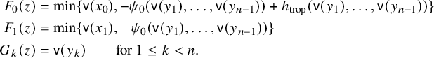 $$\begin{align*}\begin{aligned} F_0(z)&=\min\{ \operatorname{\mathrm{\mathsf{v}}}(x_0), -\psi_0(\operatorname{\mathrm{\mathsf{v}}}(y_1),\dots, \operatorname{\mathrm{\mathsf{v}}}(y_{n-1}) )+h_{\mathrm{trop}}(\mathsf v(y_1),\dots, \mathsf v(y_{n-1})) \} \\ F_1(z)&= \min \{ \operatorname{\mathrm{\mathsf{v}}}(x_1), \ \ \ \psi_0(\operatorname{\mathrm{\mathsf{v}}}(y_1),\dots, \operatorname{\mathrm{\mathsf{v}}}(y_{n-1})) \} \\ G_k(z)&=\operatorname{\mathrm{\mathsf{v}}}(y_k) \qquad \text{for} \ 1\le k< n. \end{aligned} \end{align*}$$
This is only a slight modification of (28) with $h_{\mathrm {trop}}$
in (61) replacing
$h_{\mathrm {trop}}$
in (61) replacing $\min \{0,q_1,\dots , q_{n-1}\}$
. Now, we define
$\min \{0,q_1,\dots , q_{n-1}\}$
. Now, we define $F:=(F_0,F_1, G_1,\dots , G_{n-1}): Y\to \mathbb R^{n+1}$
. One can similarly describe the image of F as before in §3.2.1. Roughly, the image
$F:=(F_0,F_1, G_1,\dots , G_{n-1}): Y\to \mathbb R^{n+1}$
. One can similarly describe the image of F as before in §3.2.1. Roughly, the image $\mathfrak B=F(Y)$
also takes the form of (29) as is the union of all
$\mathfrak B=F(Y)$
also takes the form of (29) as is the union of all $S_{\bar q}\times \{\bar q\}$
in
$S_{\bar q}\times \{\bar q\}$
in $\mathbb R^{n+1}$
, but the broken line
$\mathbb R^{n+1}$
, but the broken line $s_{\bar q}$
in (30) is modified by replacing
$s_{\bar q}$
in (30) is modified by replacing $\min \{0,\bar q\}$
by
$\min \{0,\bar q\}$
by $h_{\mathrm {trop}}$
. The image
$h_{\mathrm {trop}}$
. The image $j(B)$
then agrees with the open subset
$j(B)$
then agrees with the open subset $\hat B=\{(u_0,u_1,\bar q)\in \mathfrak B\mid u_1>0\}$
, and j exactly sends the singular locus
$\hat B=\{(u_0,u_1,\bar q)\in \mathfrak B\mid u_1>0\}$
, and j exactly sends the singular locus $\Delta $
of
$\Delta $
of $\pi $
to the singular locus of F as in Lemma 3.3. Just like §3.3, we define
$\pi $
to the singular locus of F as in Lemma 3.3. Just like §3.3, we define $\mathscr Y=F^{-1}(\hat B)$
and
$\mathscr Y=F^{-1}(\hat B)$
and $f=j^{-1}\circ F:\mathscr Y\to B$
; also, the restriction
$f=j^{-1}\circ F:\mathscr Y\to B$
; also, the restriction $f_0:=f|_{B_0}$
gives an affinoid torus fibration. In the end, the proof of Theorem 5.4 can be repeated verbatim here, obtaining
$f_0:=f|_{B_0}$
gives an affinoid torus fibration. In the end, the proof of Theorem 5.4 can be repeated verbatim here, obtaining $F\circ g=j\circ \pi _0^\vee $
and thus
$F\circ g=j\circ \pi _0^\vee $
and thus $\pi _0^\vee =f_0\circ g$
. This completes the proof of Theorem 1.12.
$\pi _0^\vee =f_0\circ g$
. This completes the proof of Theorem 1.12.
A Folklore conjecture for the critical values of Landau-Ginzburg models
In this appendix, we check some computations for the well-known folklore Conjecture II as mentioned in §1.7. A conceptual proof of the folklore conjecture is also given in [Reference Yuan62] with much generalities. We recommend a brief reading of §4 in advance.
A.1 General aspects
Let $(X_0^\vee ,\pi _0^\vee , W_0^\vee )$
be given in Theorem 4.1, and we often omit the subscript
$(X_0^\vee ,\pi _0^\vee , W_0^\vee )$
be given in Theorem 4.1, and we often omit the subscript $0$
if there is no confusion. By Remark 4.5, the superpotential should be (locally) viewed as a formal power series in
$0$
if there is no confusion. By Remark 4.5, the superpotential should be (locally) viewed as a formal power series in $\Lambda [[\pi _1(L_{q_0})]]$
for some base point
$\Lambda [[\pi _1(L_{q_0})]]$
for some base point ${q_0}$
. In general, let’s take an arbitrary formal power series
${q_0}$
. In general, let’s take an arbitrary formal power series $F=\sum _{j=1}^\infty c_jY^{\alpha _j}$
in
$F=\sum _{j=1}^\infty c_jY^{\alpha _j}$
in $\Lambda [[\pi _1(L_{q_0})]]$
for
$\Lambda [[\pi _1(L_{q_0})]]$
for $c_j\in \Lambda $
and
$c_j\in \Lambda $
and $\alpha _j\in \pi _1(L_{q_0})$
. Given
$\alpha _j\in \pi _1(L_{q_0})$
. Given $\theta \in H^1(L_{q_0})\cong \operatorname {\mathrm {Hom}} (\pi _1(L_{q_0}),\mathbb R)$
, we define the logarithmic derivative along
$\theta \in H^1(L_{q_0})\cong \operatorname {\mathrm {Hom}} (\pi _1(L_{q_0}),\mathbb R)$
, we define the logarithmic derivative along $\theta $
of F by
$\theta $
of F by
 $$\begin{align*}\textstyle D_\theta F=\sum_{j=1}^\infty c_j \langle \alpha_j, \theta\rangle Y^{\alpha_j}. \end{align*}$$
By §4.2, we take a local affinoid tropical chart of the affinoid torus fibration $\pi _0^\vee $
 $$\begin{align*}\tau: (\pi_0^\vee)^{-1}(U)\cong \operatorname{\mathrm{\mathfrak{trop}}}^{-1}(V-c) \end{align*}$$
that covers a pointed integral affine chart $\chi :(U,q_0)\to (V,c)$
. By §4.5, the superpotential
$\chi :(U,q_0)\to (V,c)$
. By §4.5, the superpotential $W^\vee $
in this chart is given by
$W^\vee $
in this chart is given by
 $$\begin{align*}W^\vee|_\tau(\mathbf y)=\sum_{\beta\in \pi_2(X,L_q) , \ \mu(\beta)=2} T^{E(\beta)} \mathbf y^{\partial\beta} \mathsf n_{\beta(q_0)} \end{align*}$$
for $\mathbf y\in H^1(L_q; U_\Lambda )$
with
$\mathbf y\in H^1(L_q; U_\Lambda )$
with $q\in U$
. Its logarithmic derivative along
$q\in U$
. Its logarithmic derivative along $\theta =\theta _q\in H^1(L_q; \mathbb R)$
is given by
$\theta =\theta _q\in H^1(L_q; \mathbb R)$
is given by
 $$\begin{align*}D_\theta W^\vee|_\tau (\mathbf y)=\sum_{\mu(\beta)=2} \langle \partial\beta, \theta\rangle T^{E(\beta)} \mathbf y^{\partial\beta} \mathsf n_{\beta(q_0)}. \end{align*}$$
Definition A.1. A point $\mathbf y$
in
$\mathbf y$
in $H^1(L_q; U_\Lambda )\subset X_0^\vee $
is called a critical point of
$H^1(L_q; U_\Lambda )\subset X_0^\vee $
is called a critical point of $W^\vee $
if
$W^\vee $
if $D_\theta W^\vee |_\tau (\mathbf y)=0$
for all
$D_\theta W^\vee |_\tau (\mathbf y)=0$
for all $\theta $
and for some affinoid tropical chart
$\theta $
and for some affinoid tropical chart $\tau $
.
$\tau $
.
This definition does not depend on the choice of the affinoid tropical chart $\tau $
as proved in [Reference Yuan62]. So, we often omit writing the
$\tau $
as proved in [Reference Yuan62]. So, we often omit writing the $\tau $
in the notations. In our situation, we just have two affinoid tropical charts:
$\tau $
in the notations. In our situation, we just have two affinoid tropical charts:
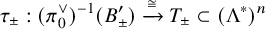 $$\begin{align*}\tau_\pm: (\pi_0^\vee)^{-1}(B^{\prime}_\pm) \xrightarrow{\cong} T_\pm \subset (\Lambda^*)^n \end{align*}$$
as in (44, 45). We will use $\overline X$
to denote a compactification of X and use
$\overline X$
to denote a compactification of X and use $W^\vee $
to denote the consequent LG superpotential. Denote by
$W^\vee $
to denote the consequent LG superpotential. Denote by $W^\vee _{\pm }:=W^\vee _{\overline X, \pm }$
the restrictions of
$W^\vee _{\pm }:=W^\vee _{\overline X, \pm }$
the restrictions of $W^\vee $
on
$W^\vee $
on $(\pi _0^\vee )^{-1}(B^{\prime }_\pm )$
.
$(\pi _0^\vee )^{-1}(B^{\prime }_\pm )$
.
The superpotential on the Clifford chamber $T_+$
is usually easy to find by [Reference Cho and Oh21]. The superpotential on the Chekanov chamber
$T_+$
is usually easy to find by [Reference Cho and Oh21]. The superpotential on the Chekanov chamber $T_-$
is hard to compute by the classic ideas. But, it can be now computed by the superpotential-preserving property (43) of the family Floer gluing maps as did in [Reference Yuan63]. Another approach over
$T_-$
is hard to compute by the classic ideas. But, it can be now computed by the superpotential-preserving property (43) of the family Floer gluing maps as did in [Reference Yuan63]. Another approach over $\mathbb C$
using the Lagrangian mutations has been studied in [Reference Pascaleff and Tonkonog54]. However, the computations in [Reference Yuan63] over
$\mathbb C$
using the Lagrangian mutations has been studied in [Reference Pascaleff and Tonkonog54]. However, the computations in [Reference Yuan63] over $\Lambda $
rather than over
$\Lambda $
rather than over $\mathbb C$
is crucial to check the folklore conjecture.
$\mathbb C$
is crucial to check the folklore conjecture.
A.2 Examples
For clarity, we only study the case $X=\mathbb C^n\setminus \mathscr D$
as in Theorem 1.5. But, one may obtain many other computations in the case of Theorem 1.12 using similar arguments.
$X=\mathbb C^n\setminus \mathscr D$
as in Theorem 1.5. But, one may obtain many other computations in the case of Theorem 1.12 using similar arguments.
A.2.1
Assume $\overline X=\mathbb {CP}^n$
. There is a topological disk
$\overline X=\mathbb {CP}^n$
. There is a topological disk $\beta '\equiv \beta '(q) \in \pi _2(\mathbb {CP}^n, L_q)$
that intersects the divisor
$\beta '\equiv \beta '(q) \in \pi _2(\mathbb {CP}^n, L_q)$
that intersects the divisor $\mathbb {CP}^n\setminus \mathbb C^n$
once and satisfies
$\mathbb {CP}^n\setminus \mathbb C^n$
once and satisfies
 $$ \begin{align} \beta'=\mathcal H-\beta_1-\cdots -\beta_n, \end{align} $$
where $\mathcal H$
is the complex line that generates
$\mathcal H$
is the complex line that generates $\pi _2(\mathbb {CP}^n)$
. We also view
$\pi _2(\mathbb {CP}^n)$
. We also view $\beta '$
as a local section of
$\beta '$
as a local section of $\mathscr R_2$
in (12) over
$\mathscr R_2$
in (12) over $B^{\prime }_+$
. Adding an extra subscript to distinguish, we use
$B^{\prime }_+$
. Adding an extra subscript to distinguish, we use $W^\vee _{\mathbb C^n,\pm }$
to denote the superpotentials obtained before in (51). First, by [Reference Cho and Oh21], the superpotential over
$W^\vee _{\mathbb C^n,\pm }$
to denote the superpotentials obtained before in (51). First, by [Reference Cho and Oh21], the superpotential over $B^{\prime }_+$
is easy to find:
$B^{\prime }_+$
is easy to find:
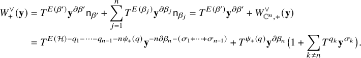 $$ \begin{align*} \begin{aligned} W^\vee_{+} (\mathbf y) &= T^{E(\beta')} \mathbf y^{\partial\beta'} \mathsf n_{\beta'} + \sum_{j=1}^n T^{E(\beta_j)} \mathbf y^{\partial\beta_j} \mathsf n_{\beta_j} = T^{E(\beta')} \mathbf y^{\partial\beta'} + W_{\mathbb C^n,+}^\vee (\mathbf y) \\ &= T^{E(\mathcal H) -q_1-\cdots -q_{n-1}-n\psi_+(q)} \mathbf y^{-n\partial\beta_n-(\sigma_1+\cdots +\sigma_{n-1})} + T^{\psi_+(q)} \mathbf y^{\partial\beta_n} \big(1+ \sum_{k\neq n} T^{q_k} \mathbf y^{\sigma_k}\big). \end{aligned} \end{align*} $$
We can also use [Reference Cho and Oh21] again to conclude $\mathsf n_{\beta '}=1$
. By [Reference Yuan63], the superpotential over
$\mathsf n_{\beta '}=1$
. By [Reference Yuan63], the superpotential over $B^{\prime }_-$
is
$B^{\prime }_-$
is
 $$ \begin{align} W^\vee_{-}( {\mathbf y}) = T^{\psi_-} {\mathbf y}^{\partial\hat\beta} + T^{-n\psi_-+E(\mathcal H)} {\mathbf y}^{-n\partial\hat\beta-(\sigma_1+\cdots+\sigma_{n-1})}\big(1+T^{q_1} {\mathbf y}^{\sigma_1}+\cdots+ T^{q_{n-1}} {\mathbf y}^{\sigma_{n-1}} \big)^n. \end{align} $$
Under the identifications $(\pi _0^\vee )^{-1}(B^{\prime }_\pm )\cong T_\pm $
via
$(\pi _0^\vee )^{-1}(B^{\prime }_\pm )\cong T_\pm $
via $\tau _\pm $
, they have the following expressions: For
$\tau _\pm $
, they have the following expressions: For ${y=(y_1,\dots , y_n)}$
in
${y=(y_1,\dots , y_n)}$
in $T_+$
or
$T_+$
or $T_-$
, we respectively have
$T_-$
, we respectively have
 $$ \begin{align} \begin{aligned} W^\vee_+ (y) &= y_n(1+y_1+\cdots+y_{n-1}) + \frac{T^{E(\mathcal H)}}{y_1\cdots y_{n-1} \cdot y_n^n} \\ W^\vee_- (y) &= y_n + \frac{T^{E(\mathcal H)}(1+y_1+\cdots + y_{n-1})^n}{y_1\cdots y_{n-1}\cdot y_n^n}. \ \end{aligned} \end{align} $$
Moreover, under the analytic embedding g in (58) into the $\Lambda $
-variety
$\Lambda $
-variety
 $$\begin{align*}Y=\{ \pmb z=(x_0,x_1,y_1,\dots, y_{n-1}) \in \Lambda^2\times (\Lambda^*)^{n-1} \mid x_0x_1=1+y_1+\cdots +y_{n-1} \}, \end{align*}$$
we can check that the $W_\pm ^\vee $
together give rise to a single expression
$W_\pm ^\vee $
together give rise to a single expression
 $$ \begin{align} W^\vee (\pmb z) = x_1+\frac{T^{E(\mathcal H)} \cdot x_0^n}{ y_1\cdots y_{n-1}}. \end{align} $$
It is first only defined on a subdomain $\mathscr Y_0$
in Y; but thanks to Theorem 1.5, its domain can be extended to the whole Y.
$\mathscr Y_0$
in Y; but thanks to Theorem 1.5, its domain can be extended to the whole Y.
Next, we aim to find the critical points of $W^\vee $
. The methods are not unique. For instance, we may use various tropical charts of Y in the sense of [Reference Chambert-Loir and Ducros14, §3] (cf. the recent [Reference Gubler, Jell and Rabinoff43]). The critical points are actually coordinate-free. Anyway, for clarity, let’s use the two familiar charts
$W^\vee $
. The methods are not unique. For instance, we may use various tropical charts of Y in the sense of [Reference Chambert-Loir and Ducros14, §3] (cf. the recent [Reference Gubler, Jell and Rabinoff43]). The critical points are actually coordinate-free. Anyway, for clarity, let’s use the two familiar charts $\tau _\pm $
.
$\tau _\pm $
.
-
• In the affinoid tropical chart
$\tau _+$
, we have for
$$ \begin{align*} D_k W^\vee_+ &= - \frac{T^{E(\mathcal H)} }{y_1\cdots y_{n-1} y_n^n} + y_ny_k && 1\le k <n \\ D_n W^\vee_+ &= -\frac{n \ T^{E(\mathcal H)}}{y_1\cdots y_{n-1} y_n^n} + y_n(1+y_1+\cdots +y_{n-1}) \end{align*} $$
$y=(y_1,\dots , y_n)\in T_+$
. Then, we can solve and obtain the critical points (if exist in
$T_+$
): The corresponding critical values are
$$\begin{align*}\begin{cases} y_k=1 & 1\le k<n \\ y_n= T^{\frac{1}{n+1} E(\mathcal H)} e^{\frac{2\pi i s}{n+1}} & s\in \{0,1,\dots, n\}. \end{cases} \end{align*}$$
$(n+1)T^{\frac {1}{n+1} E(\mathcal H)} e^{\frac {2\pi i s}{n+1}}$
.
-
• In the affinoid tropical chart
$\tau _-$
, we also have for
$$ \begin{align*} D_k W_-^\vee &= -\frac{T^{E(\mathcal H)} (1+y_1+\cdots +y_{n-1})^n }{y_1\cdots y_{n-1} y_n^n} + n \frac{T^{E(\mathcal H)} (1+y_1+\cdots +y_{n-1})^{n-1} y_k}{y_1\cdots y_{n-1}y_n^n} \\ D_n W_-^\vee &= y_n - \frac{n T^{E(\mathcal H)} (1+y_1+\cdots +y_{n-1})^n}{y_1\cdots y_{n-1}y_n^n} \end{align*} $$
$y=(y_1,\dots , y_n)\in T_-$
. Then, we can solve and obtain the critical points (if any): The corresponding critical values are also
$$\begin{align*}\begin{cases} y_k=1 & 1\le k < n \\ y_n = nT^{\frac{1}{n+1} E(\mathcal H)} e^{\frac{2\pi i s}{n+1}} & s\in\{0,1,\dots, n\}. \end{cases} \end{align*}$$
$(n+1)T^{\frac {1}{n+1} E(\mathcal H)} e^{\frac {2\pi i s}{n+1}}$
.


In either case, the critical values agree with the known eigenvalues of the quantum product in $\mathbb {CP}^n$
of the first Chern class. Under the analytic embedding g, the critical points in either bullets have the uniform expressions as follows:
$\mathbb {CP}^n$
of the first Chern class. Under the analytic embedding g, the critical points in either bullets have the uniform expressions as follows:
 $$\begin{align*}\mathbf{z}^{(s)} =(x_0,x_1,y_1,\dots, y_{n-1}) \ \in Y: \qquad \begin{cases} x_0 = T^{-\frac{E(\mathcal H)}{n+1}} e^{-\frac{2\pi i s}{n+1}} & \\ x_1 = n T^{\frac{E(\mathcal H)}{n+1} } e^{\frac{2\pi i s}{n+1}} & \\ y_k =1 & 1\le k<n \end{cases} \end{align*}$$
for $s\in \{0,1,\dots , n\}$
. Since
$s\in \{0,1,\dots , n\}$
. Since $\operatorname {\mathrm {\mathsf {v}}}(y_k)=0$
, the critical points are all contained in the dual fiber over a fixed single point
$\operatorname {\mathrm {\mathsf {v}}}(y_k)=0$
, the critical points are all contained in the dual fiber over a fixed single point $\hat q=(0,\dots , 0, a_\omega )$
in
$\hat q=(0,\dots , 0, a_\omega )$
in $B\equiv \mathbb R^n$
for some
$B\equiv \mathbb R^n$
for some $a_\omega \in \mathbb R$
, and
$a_\omega \in \mathbb R$
, and $\operatorname {\mathrm {\mathsf {v}}}(x_1)=\psi (\hat q)=\frac {1}{n+1}E(\mathcal H)=\frac {1}{2\pi (n+1)}\omega (\mathcal H)$
. In particular, the Kähler form
$\operatorname {\mathrm {\mathsf {v}}}(x_1)=\psi (\hat q)=\frac {1}{n+1}E(\mathcal H)=\frac {1}{2\pi (n+1)}\omega (\mathcal H)$
. In particular, the Kähler form $\omega $
determines
$\omega $
determines $a_\omega $
and the base point
$a_\omega $
and the base point $\hat q$
. Besides, the critical points are in
$\hat q$
. Besides, the critical points are in $T_+$
if
$T_+$
if $a_\omega>0$
and in
$a_\omega>0$
and in $T_-$
if
$T_-$
if $a_\omega <0$
. But, it is not completely clear when
$a_\omega <0$
. But, it is not completely clear when $a_\omega =0$
and
$a_\omega =0$
and $\hat q$
lies on the singular locus.
$\hat q$
lies on the singular locus.
A.2.2
Assume $\overline X=\mathbb {CP}^m\times \mathbb {CP}^{n-m}$
for
$\overline X=\mathbb {CP}^m\times \mathbb {CP}^{n-m}$
for $1\le m <n$
. Let
$1\le m <n$
. Let $\mathcal H_1$
(resp.
$\mathcal H_1$
(resp. $\mathcal H_2$
) be the class of a complex line in
$\mathcal H_2$
) be the class of a complex line in $\mathbb {CP}^m$
(resp.
$\mathbb {CP}^m$
(resp. $\mathbb {CP}^{n-m}$
). There are two new disk classes
$\mathbb {CP}^{n-m}$
). There are two new disk classes $\beta ^{\prime }_1$
and
$\beta ^{\prime }_1$
and $\beta ^{\prime }_2$
bounding the
$\beta ^{\prime }_2$
bounding the $\pi $
-fibers over
$\pi $
-fibers over $B_+$
. Besides,
$B_+$
. Besides, $\mathcal H_1=\beta ^{\prime }_1+\sum _{i=1}^m \beta _i$
and
$\mathcal H_1=\beta ^{\prime }_1+\sum _{i=1}^m \beta _i$
and $\mathcal H_2=\beta ^{\prime }_2+\sum _{i=m+1}^n \beta _i$
. One can finally show that the superpotential under the analytic embedding g is given by
$\mathcal H_2=\beta ^{\prime }_2+\sum _{i=m+1}^n \beta _i$
. One can finally show that the superpotential under the analytic embedding g is given by
 $$\begin{align*}W^\vee (\pmb z) = x_1 + \frac{T^{E(\mathcal H_1)} x_0^m}{y_1\cdots y_m} + \frac{T^{E(\mathcal H_2)} x_0^{n-m}}{ y_{m+1}\cdots y_{n-1}} \end{align*}$$
for $\pmb z=(x_0,x_1,y_1,\dots , y_{n-1})$
on the same variety Y. We have
$\pmb z=(x_0,x_1,y_1,\dots , y_{n-1})$
on the same variety Y. We have $(m+1)(n-m+1)$
critical points
$(m+1)(n-m+1)$
critical points
 $$\begin{align*}\begin{cases} x_0 = \big( T^{\frac{E(\mathcal H_2)}{n-m+1}} e^{\frac{2\pi i s}{n-m+1}} \big)^{-1} & \\ x_1 = T^{\frac{E(\mathcal H_2)}{n-m+1}} e^{\frac{2\pi i s}{n-m+1}} \cdot \left(m \ T^{\frac{E(\mathcal H_1)}{m+1}} e^{\frac{2\pi i r}{m+1}} \cdot \big( T^{\frac{E(\mathcal H_2)}{n-m+1}} e^{\frac{2\pi i s}{n-m+1}} \big)^{-1}+ n-m\right) & \\ y_k = T^{\frac{E(\mathcal H_1)}{m+1}} e^{\frac{2\pi i r}{m+1}} \cdot \big( T^{\frac{E(\mathcal H_2)}{n-m+1}} e^{\frac{2\pi i s}{n-m+1}} \big)^{-1} & 1\le k\le m \\ y_\ell= 1 & m< \ell <n \end{cases} \end{align*}$$
for $r\in \{0,1,\dots , m\}$
and
$r\in \{0,1,\dots , m\}$
and $s\in \{0,1,\dots , n-m\}$
. Then, the corresponding critical values are
$s\in \{0,1,\dots , n-m\}$
. Then, the corresponding critical values are
 $$\begin{align*}(m+1) T^{\frac{E(\mathcal H_1)}{m+1}} e^{\frac{2\pi i r}{m+1}} + (n-m+1) T^{\frac{E(\mathcal H_2)}{n-m+1}} e^{\frac{2\pi i s}{n-m+1}}. \end{align*}$$
Let’s further look into a special case when $m=1$
and
$m=1$
and $n=2$
. Namely,
$n=2$
. Namely, $\overline X=\mathbb {CP}^1\times \mathbb {CP}^1$
. Then,
$\overline X=\mathbb {CP}^1\times \mathbb {CP}^1$
. Then,
 $$\begin{align*}W^\vee=x_1+ \frac{T^{E(\mathcal H_1)}x_0}{y_1}+{T^{E(\mathcal H_2)} x_0}. \end{align*}$$
By the above computation, we have four critical points given by
 $$\begin{align*}\begin{cases} x_0=\big( T^{\frac{E(\mathcal H_2)}{2}} e^{\pi i s} \big)^{-1} \\ x_1= T^{\frac{E(\mathcal H_2)}{2}} e^{\pi i s} \big( T^{\frac{E(\mathcal H_1)-E(\mathcal H_2)}{2}} e^{\pi i s} e^{\pi i r} +1 \big) \\ y_1=T^{\frac{E(\mathcal H_1)-E(\mathcal H_2)}{2}} e^{\pi i r} e^{\pi i s} \end{cases} \end{align*}$$
for $r,s\in \{0,1\}$
. The base point in
$r,s\in \{0,1\}$
. The base point in $B\equiv \mathbb R^2$
is given by
$B\equiv \mathbb R^2$
is given by $ \hat q=\left ( \frac {E(\mathcal H_1)-E(\mathcal H_2)}{2}, a_\omega \right ) $
for some
$ \hat q=\left ( \frac {E(\mathcal H_1)-E(\mathcal H_2)}{2}, a_\omega \right ) $
for some $a_\omega \in \mathbb R$
. More examples can be similarly found out by either choosing a different compactification
$a_\omega \in \mathbb R$
. More examples can be similarly found out by either choosing a different compactification $\overline X$
or working with a more general X as Theorem 1.12; compare also [Reference Yuan63].
$\overline X$
or working with a more general X as Theorem 1.12; compare also [Reference Yuan63].
Acknowledgements
We thank Mohammed Abouzaid for encouraging discussions about [Reference Abouzaid and Sylvan2]. We thank Denis Auroux and Yingdi Qin for some key ideas for Lemma 2.4. We thank Antoine Chambert-Loir for a correspondence that explains [Reference Chambert-Loir and Ducros14], especially the notion of the tropically continuous map. We thank Jonathan David Evans for a helpful correspondence about [Reference Evans28]. We thank Kenji Fukaya and Eric Zaslow for their interests, conversations and supports. We thank Siu-Cheong Lau for a useful correspondence about [Reference Hong, Kim and Lau45]. We thank Yang Li for his interest and useful discussion. We thank Enrica Mazzon and Yueqiao Wu for patient explanations of the basics of Berkovich’s theory. We thank Sam Payne for a helpful explanation of [Reference Payne55]. We thank Tony Yue Yu for an insightful suggestion of Section 8 of Kontsevich-Soibelman’s paper [Reference Kontsevich and Soibelman50] and for many useful lessons of non-archimedean geometry.
Competing interests
The authors have no competing interest to declare.


 Open access